





1. Introduction
Transport of heat and chemical species in porous media is relevant to natural and industrial flows: from latent heat thermal energy storage systems (Trelles & Dufly Reference Trelles and Dufly2003; Xu et al. Reference Xu, Ren, Zheng and He2017) to the formation of sea ice (Feltham et al. Reference Feltham, Untersteiner, Wettlaufer and Worster2006; Wells, Hitchen & Parkinson Reference Wells, Hitchen and Parkinson2019), several key processes are controlled by the redistribution of heat and solutes in confined domains. When the motion is driven by density gradients within the fluid layer, and the density field depends on the local distribution of the scalar (e.g. temperature or solute concentration), the flow is controlled by natural convection. In porous-media convection, the governing equations for thermally driven and solute-driven flows are equivalent once expressed in dimensionless form, with temperature and solute concentration playing analogous roles as buoyancy-driving scalars. As a result, insights obtained from one formulation can be directly transferred to the other. In the present work, we adopt a thermal formulation of the problem, which provides a convenient and widely used framework while retaining full relevance for solutal convection applications. In convective flows, local density differences are contrasted by the dissipative mechanisms of friction (due to narrow pore spaces) and diffusion (which reduce the gradients of the scalar field), which, in turn, affect the flow field. The relative importance of driving (convection) and dissipative (diffusion, friction) mechanisms is quantified by the Rayleigh–Darcy number $Ra$
(hereinafter defined as Rayleigh number). A similar dynamics occurs in the presence of key geophysical systems, where buoyancy is induced by solute concentration gradients rather than temperature variations, e.g. geothermal flows in underground sites (Hu, Xu & Yang Reference Hu, Xu and Yang2023), thawing of permafrost (Wang et al. Reference Wang, Xie, Yang, Li, Abulaiti, Zheng, Zhu and Xu2025), dispersion of contaminants in groundwater flows (Simmons, Fenstemaker & Sharp Reference Simmons, Fenstemaker and Sharp2001; De Paoli et al. Reference De Paoli, Yerragolam, Verzicco and Lohse2025b
) and storage of carbon dioxide (CO
$Ra$
(hereinafter defined as Rayleigh number). A similar dynamics occurs in the presence of key geophysical systems, where buoyancy is induced by solute concentration gradients rather than temperature variations, e.g. geothermal flows in underground sites (Hu, Xu & Yang Reference Hu, Xu and Yang2023), thawing of permafrost (Wang et al. Reference Wang, Xie, Yang, Li, Abulaiti, Zheng, Zhu and Xu2025), dispersion of contaminants in groundwater flows (Simmons, Fenstemaker & Sharp Reference Simmons, Fenstemaker and Sharp2001; De Paoli et al. Reference De Paoli, Yerragolam, Verzicco and Lohse2025b
) and storage of carbon dioxide (CO $_2$
) in saline aquifers. The latter, in particular, has been extensively studied in recent decades, due to its enormous relevance in mitigating the effects of climate change (Metz et al. Reference Metz2005). Geological sequestration of CO
$_2$
) in saline aquifers. The latter, in particular, has been extensively studied in recent decades, due to its enormous relevance in mitigating the effects of climate change (Metz et al. Reference Metz2005). Geological sequestration of CO $_2$
involves injecting large amounts of CO
$_2$
involves injecting large amounts of CO $_2$
into underground geological porous formations for permanent storage (Emami-Meybodi et al. Reference Emami-Meybodi, Hassanzadeh, Green and Ennis-King2015; Jin Reference Jin2024). A key question in assessing the suitability of potential sequestration sites is determining the CO
$_2$
into underground geological porous formations for permanent storage (Emami-Meybodi et al. Reference Emami-Meybodi, Hassanzadeh, Green and Ennis-King2015; Jin Reference Jin2024). A key question in assessing the suitability of potential sequestration sites is determining the CO $_2$
mixing rate in brine.
$_2$
mixing rate in brine.
Although the physical motivation for this study is rooted in solutal convection relevant to CO $_2$
sequestration, the analysis presented here is carried out using a thermal formulation. Owing to the formal equivalence between thermal and solutal convection in porous media, all results can be directly reinterpreted in terms of mass transfer, with the dimensionless governing and response parameters retaining the same physical meaning. The archetypal system used to analyse this problem is the one-sided (or semi-infinite) configuration (Hidalgo et al. Reference Hidalgo, Fe, Cueto-Felgueroso and Juanes2012): the flow is idealised as a rectangular box, initially filled with low-density fluid (representing brine). At the top boundary (representing the CO
$_2$
sequestration, the analysis presented here is carried out using a thermal formulation. Owing to the formal equivalence between thermal and solutal convection in porous media, all results can be directly reinterpreted in terms of mass transfer, with the dimensionless governing and response parameters retaining the same physical meaning. The archetypal system used to analyse this problem is the one-sided (or semi-infinite) configuration (Hidalgo et al. Reference Hidalgo, Fe, Cueto-Felgueroso and Juanes2012): the flow is idealised as a rectangular box, initially filled with low-density fluid (representing brine). At the top boundary (representing the CO $_2$
–brine interface) the fluid density is maximum (Jin Reference Jin2024). At the bottom boundary, the domain is assumed to be closed due to the presence of an impermeable rock layer. The flow dynamics that takes place is marked by a transient behaviour, controlled by the convective flow structures that populate the system. Numerical simulations have been extensively deployed to analyse these flows (Hewitt, Neufeld & Lister Reference Hewitt, Neufeld and Lister2013; Slim Reference Slim2014; Wen et al. Reference Wen, Akhbari, Zhang and Hesse2018). Despite these efforts, several research questions remain unanswered. For sufficiently large domains and high values of Rayleigh numbers, the flow evolution is still transient, but it is also independent of the domain size and
$_2$
–brine interface) the fluid density is maximum (Jin Reference Jin2024). At the bottom boundary, the domain is assumed to be closed due to the presence of an impermeable rock layer. The flow dynamics that takes place is marked by a transient behaviour, controlled by the convective flow structures that populate the system. Numerical simulations have been extensively deployed to analyse these flows (Hewitt, Neufeld & Lister Reference Hewitt, Neufeld and Lister2013; Slim Reference Slim2014; Wen et al. Reference Wen, Akhbari, Zhang and Hesse2018). Despite these efforts, several research questions remain unanswered. For sufficiently large domains and high values of Rayleigh numbers, the flow evolution is still transient, but it is also independent of the domain size and $Ra$
(De Paoli et al. Reference De Paoli, Zonta, Enzenberger, Coliban and Pirozzoli2025d
). What is the minimal flow unit required to achieve such a self-similar behaviour? And what is the effect of the domain size on the mixing properties of the flow? In this work, we answer these questions by systematically analysing the effects of the domain size and of the Rayleigh number
$Ra$
(De Paoli et al. Reference De Paoli, Zonta, Enzenberger, Coliban and Pirozzoli2025d
). What is the minimal flow unit required to achieve such a self-similar behaviour? And what is the effect of the domain size on the mixing properties of the flow? In this work, we answer these questions by systematically analysing the effects of the domain size and of the Rayleigh number $Ra$
of the emerging flow patterns.
$Ra$
of the emerging flow patterns.
The one-sided configuration described above presents a major drawback: it is intrinsically transient, which markedly complicates any theoretical analysis of the flow. In contrast, the ‘two-sided’ (Rayleigh–Bénard) configuration, in which the fluid density is fixed at the top and also at the bottom, attains a (statistically) steady state, which makes it more suitable for theoretical analysis. In addition, it has been shown (Hewitt et al. Reference Hewitt, Neufeld and Lister2013) that the two-sided flow is directly related to the one-sided configuration during the late-stage dynamics, indicated as the ‘shutdown of convection’ and corresponding to a well-mixed bulk flow configuration. The two-sided system is well defined in terms of boundary conditions, and during the statistically steady state, it is possible to derive exact equations that describe the flow transport properties as a function of the governing parameters (Grossmann & Lohse Reference Grossmann and Lohse2000, Reference Grossmann and Lohse2001; Lohse & Shishkina Reference Lohse and Shishkina2024). For these reasons, a number of works (Hewitt, Neufeld & Lister Reference Hewitt, Neufeld and Lister2012; Hewitt, Neufeld & Lister Reference Hewitt, Neufeld and Lister2014; Wen, Corson & Chini Reference Wen, Corson and Chini2015; De Paoli, Zonta & Soldati Reference De Paoli, Zonta and Soldati2016; Pirozzoli et al. Reference Pirozzoli, De Paoli, Zonta and Soldati2021; De Paoli et al. Reference De Paoli, Pirozzoli, Zonta and Soldati2022; Hu et al. Reference Hu, Xu and Yang2023; Zhu, Fu & De Paoli Reference Zhu, Fu and De Paoli2024) have investigated the two-sided configuration. However, several questions remain unanswered in this case as well. The near-wall flow structure organises into multiple hierarchical levels, from the small-scale (near-wall) plumes nesting into large-scale structures (labelled as ‘supercells’; De Paoli et al. Reference De Paoli, Pirozzoli, Zonta and Soldati2022), which have been only partially characterised by analysing scalar fields after applying ad hoc threshold filtering. Can the supercells be identified more robustly and univocally? Can their formation be predicted based on the values of the domain size and $Ra$
considered? Can a
$Ra$
considered? Can a $Ra$
-independent description of the near-wall small-scale structures be derived? What is the flow structure at small and large
$Ra$
-independent description of the near-wall small-scale structures be derived? What is the flow structure at small and large $Ra$
in the presence of large domains?
$Ra$
in the presence of large domains?
As a result of the complex interplay between diffusion and buoyancy, the flow structures organise into tangled, dynamic patterns, making it extremely challenging to predict and quantify their behaviour. Initial efforts in this direction include using Fourier-based analysis (Hewitt et al. Reference Hewitt, Neufeld and Lister2014; Pirozzoli et al. Reference Pirozzoli, De Paoli, Zonta and Soldati2021; De Paoli et al. Reference De Paoli, Zonta, Enzenberger, Coliban and Pirozzoli2025d ) as well as utilising cell sizes as a measure of emerging patterns (Fu, Cueto-Felgueroso & Juanes Reference Fu, Cueto-Felgueroso and Juanes2013; De Paoli et al. Reference De Paoli, Pirozzoli, Zonta and Soldati2022). However, there is much more that can be done in this direction. One approach that appears appropriate is based on topological measures, which provide an efficient and detailed analysis of structures characterised by a value of a scalar field (in this case, solute concentration). While several approaches of varying complexity can be implemented for this purpose, measures based on the exploration of the connectivity of the considered structures appear to be the most appropriate. Such approaches, based on a computational topology discipline, persistent homology (PH), have been used to analyse a variety of systems emerging from materials science, such as granular matter (Kondic et al. Reference Kondic, Goullet, O’Hern, Kramar, Mischaikow and Behringer2012; Kramár et al. Reference Kramár, Goullet, Kondic and Mischaikow2014a ,Reference Kramár, Goullet, Kondic and Mischaikow b ; Taghizadeh et al. Reference Taghizadeh, Luding, Basak and Kondic2024), Rayleigh–Bénard convection (Kramár et al. Reference Kramár, Levanger, Tithof, Suri, Xu, Paul, Schatz and Mischaikow2016), suspensions (Gameiro et al. Reference Gameiro, Singh, Kondic, Mischaikow and Morris2020) and porous media (Suzuki et al. Reference Suzuki, Miyazawa, Minto, Tsuji, Obayashi, Hiraoka and Ito2021), among others. One advantage of using PH-based measures is that they are objective in the sense that they do not require specifying a threshold value (such as average temperature or a similar quantity), but instead, they quantify the structure across all thresholds at once. We will see that PH-based approaches provide significant new information about the structures developing in the considered system, their connection to heat transport, and in particular, that they allow for answering some questions formulated so far.
The paper is organised as follows. In § 2, we present the governing equations and flow configurations considered, and discuss the equivalence between thermal and solutal formulations in porous-media convection. In § 3, we provide an overview of the PH methods used to quantify the emerging patterns. The results of the one-sided and two-sided systems analysed are presented in §§ 4 and 5, respectively. Finally, an overview of the work and conclusions are presented in § 6.
2. Governing equations
We consider convective porous media flows at the Darcy scale, i.e. the flow properties averaged over a reference elementary volume (Whitaker Reference Whitaker1998; Nield & Bejan Reference Nield and Bejan2017). In particular, we focus on density-driven flows in which the source of buoyancy is due to a temperature-induced density field, and with the solid locally in thermal equilibrium with the liquid phase. We consider thermally driven flows, as they are relevant to both the one-sided and two-sided configurations (Hu et al. Reference Hu, Xu and Yang2023). However, the same dimensionless equations apply to solutal convection. The governing equations in dimensional and dimensionless form are presented in §§ 2.1 and 2.2, respectively, and the data analysed are discussed in § 2.3.
Temperature distribution over the surface of the domain, with indication of the dimensional extension in each direction ( $L_1^*,L_2^*,H^*$
) and of the boundary conditions. (a) One-sided flow configuration, discussed in § 4. (b) Two-sided flow configuration, discussed in § 5.
$L_1^*,L_2^*,H^*$
) and of the boundary conditions. (a) One-sided flow configuration, discussed in § 4. (b) Two-sided flow configuration, discussed in § 5.

Figure 1. Long description
Panel A: A 3D diagram of one-sided flow configuration. The diagram shows a cube with the top surface labeled T* equals T* min in blue and the bottom surface with a gradient from red to dark red. The axes are labeled H*, L2*, and L1*. The temperature gradient dT* over dz* at z* equals 0 is indicated with a blue arrow. Panel B: A 3D diagram of two-sided flow configuration. The diagram shows a cube with the top surface labeled T* equals T* min in black and the bottom surface with a gradient from yellow to red. The axes are labeled H*, L2*, and L1*. The temperature at z* equals 0 is indicated as T* max with a red arrow.
2.1. Problem formulation
We consider a three-dimensional (3-D) porous domain with uniform porosity $\phi$
and permeability
$\phi$
and permeability $K$
. The medium is fully saturated with fluid, whose density depends on the temperature field,
$K$
. The medium is fully saturated with fluid, whose density depends on the temperature field, $T^*$
. The local gradients of fluid density within the system drive the flow. Figure 1 shows a sketch of the domain; here, two different flow configurations, discussed in detail in the following, are described.
$T^*$
. The local gradients of fluid density within the system drive the flow. Figure 1 shows a sketch of the domain; here, two different flow configurations, discussed in detail in the following, are described.
We indicate by $x^*$
and
$x^*$
and $y^*$
the horizontal directions and by
$y^*$
the horizontal directions and by $z^*$
the vertical direction (perpendicular to the walls) along which the gravitational acceleration
$z^*$
the vertical direction (perpendicular to the walls) along which the gravitational acceleration $\boldsymbol{g}$
is aligned. The temperature field
$\boldsymbol{g}$
is aligned. The temperature field $T^*$
, averaged over the reference elementary volume, varies between
$T^*$
, averaged over the reference elementary volume, varies between $T^*_{\textit{min}}$
and
$T^*_{\textit{min}}$
and $T^*_{\textit{max}}$
, and it is controlled by the advection–diffusion equation (Nield & Bejan Reference Nield and Bejan2017):
$T^*_{\textit{max}}$
, and it is controlled by the advection–diffusion equation (Nield & Bejan Reference Nield and Bejan2017):
 \begin{align} [(1-\phi )(\rho c)_s + \phi (\rho c)_{\!f}] \frac {\partial T^*}{\partial t^*} + (\rho c)_{\!f} \boldsymbol{u}^*\boldsymbol{\cdot }\boldsymbol{\nabla} ^* T^* = \boldsymbol{\nabla} ^*\boldsymbol{\cdot }([(1-\phi )\lambda _s + \phi \lambda _{\!f}] \boldsymbol{\nabla} ^* T^*), \end{align}
where $s$
and
$s$
and $f$
refer to the solid and fluid phases, respectively,
$f$
refer to the solid and fluid phases, respectively, $c$
is the specific heat (considered at constant pressure for the fluid) and
$c$
is the specific heat (considered at constant pressure for the fluid) and $\lambda$
the thermal conductivity (the superscript
$\lambda$
the thermal conductivity (the superscript $^{*}$
indicates dimensional variables). In this case, we consider a system in local thermal equilibrium (
$^{*}$
indicates dimensional variables). In this case, we consider a system in local thermal equilibrium ( $T_{\!f} = T_s = T$
) and without heat production. In addition, when the heat capacity of the solid is negligible (
$T_{\!f} = T_s = T$
) and without heat production. In addition, when the heat capacity of the solid is negligible ( $(\rho c)_s\to 0$
), (2.1) reduces to (Hewitt Reference Hewitt2020)
$(\rho c)_s\to 0$
), (2.1) reduces to (Hewitt Reference Hewitt2020)
 \begin{equation} \phi \frac {\partial T^*}{\partial t^*}+\boldsymbol{u}^{*}\boldsymbol{\nabla} ^{*} \boldsymbol{\cdot }T^* =\boldsymbol{\nabla} ^{*} \boldsymbol{\cdot }(\kappa \boldsymbol{\nabla} ^{*} T^*), \end{equation}
where $t^*$
is time,
$t^*$
is time, $\boldsymbol{u}^{*}=(u^{*},v^{*},w^{*})$
is the volume-averaged velocity field,
$\boldsymbol{u}^{*}=(u^{*},v^{*},w^{*})$
is the volume-averaged velocity field, $\phi$
is the porosity of the medium and
$\phi$
is the porosity of the medium and $\kappa = [(1-\phi )\lambda _s + \phi \lambda _{\!f}]/(\rho c)_{\!f}$
is the thermal diffusivity of the medium, considered constant here. The fluid density,
$\kappa = [(1-\phi )\lambda _s + \phi \lambda _{\!f}]/(\rho c)_{\!f}$
is the thermal diffusivity of the medium, considered constant here. The fluid density, $\rho ^{*}$
, is assumed to depend linearly on temperature:
$\rho ^{*}$
, is assumed to depend linearly on temperature:
 \begin{equation} \rho ^{*}(T^*)=\rho ^{*}(T^*_{\textit{min}})-\Delta \rho ^{*}\frac {T^*-T^*_{\textit{min}}}{T^*_{\textit{max}}-T^*_{\textit{min}}} \text{ ,} \end{equation}
with $\Delta \rho ^{*}=\rho ^{*}(T^*_{\textit{min}})-\rho ^{*}(T^*_{\textit{max}})$
being the maximum density contrast within the domain. Assuming the validity of the Boussinesq approximation (Landman & Schotting Reference Landman and Schotting2007), the flow field is described by the continuity and the Darcy equations,
$\Delta \rho ^{*}=\rho ^{*}(T^*_{\textit{min}})-\rho ^{*}(T^*_{\textit{max}})$
being the maximum density contrast within the domain. Assuming the validity of the Boussinesq approximation (Landman & Schotting Reference Landman and Schotting2007), the flow field is described by the continuity and the Darcy equations,
 \begin{equation} \boldsymbol{\nabla} ^{*}\boldsymbol{\cdot }\boldsymbol{u}^{*}=0,\quad \boldsymbol{u}^{*}=-\frac {K}{\mu }\left (\boldsymbol{\nabla} ^{*} P^{*}+\rho ^{*}g \boldsymbol{k}\right )\!, \end{equation}
respectively, with $\mu$
the (constant) fluid viscosity,
$\mu$
the (constant) fluid viscosity, $P^{*}$
the pressure and
$P^{*}$
the pressure and $\boldsymbol{k}$
the vertical unit vector. The walls are considered impermeable to the fluid, i.e. the following boundary conditions for the flow field apply:
$\boldsymbol{k}$
the vertical unit vector. The walls are considered impermeable to the fluid, i.e. the following boundary conditions for the flow field apply:
 \begin{equation} w^*(z^*=0)=0,\quad w^*(z^*=H^{*})=0 . \end{equation}
Note that a slip at the walls is possible, due to the Darcy formulation adopted. Periodicity is considered across the vertical boundaries (directions $x,y$
) for all flow variables.
$x,y$
) for all flow variables.
Regarding the temperature field, at the upper and lower walls, both Dirichlet ( $T^*$
fixed) or Neumann (
$T^*$
fixed) or Neumann ( $\partial T^*/\partial z^*$
fixed) boundary conditions are considered:
$\partial T^*/\partial z^*$
fixed) boundary conditions are considered:
-
(i) Semi-infinite domain: the temperature is fixed at the top and no-flux condition is assumed at the bottom (see figure 1 a), namely
(2.6)In addition, the domain is initially filled with still fluid and at temperature \begin{equation} T^*(z^*=H^*)=T^*_{\textit{min}}, \quad \frac {\partial T^*}{\partial z^*}\biggr |_{z^*=0} =0 . \end{equation}
$T^*_{\textit{max}}$
. Thus, the velocity and temperature fields are initialised as
$\boldsymbol{u^*}=0$
and(2.7)respectively. The initial condition (2.7) is obtained evaluating at time
\begin{equation} T^*(x^*,y^*,z^*\lt H^*,t_0^*)=T^*_{\textit{min}} + (T^*_{\textit{max}}-T^*_{\textit{min}})\,\text{erf}\left [\sqrt {\frac {\phi }{\kappa }}\frac {(H^*-z^*)}{2\sqrt {t^*_0}}\right ]\!, \end{equation}
$t_0^*$
the self-similar solution of (2.2) in the absence of convection (
$\boldsymbol{u}^*=0$
) in a semi-infinite domain
$(H^*\to \infty )$
(De Paoli, Zonta & Soldati Reference De Paoli, Zonta and Soldati2017). The instant considered to initialise the simulation is
$t_0^*=250 \phi \kappa (g \Delta \rho ^{*} K / \mu )^{-2}$
, corresponding to a dimensionless time of
$\widehat {t}_0=250$
or
$t_0=250/{Ra}$
, expressed in diffusive or convective units, respectively (see § 2.2 for further details). Finally, a random perturbation (white noise) is added. The amplitude of this noise controls the time at which the plumes form, i.e. the onset of convection occurs (De Paoli et al. Reference De Paoli, Zonta, Enzenberger, Coliban and Pirozzoli2025d
). This flow configuration, also labelled as ‘one-sided’, is representative of a domain cooled from above and insulated from below, and will be analysed in § 4.
\begin{equation} T^*(z^*=H^*)=T^*_{\textit{min}}, \quad \frac {\partial T^*}{\partial z^*}\biggr |_{z^*=0} =0 . \end{equation}
$T^*_{\textit{max}}$
. Thus, the velocity and temperature fields are initialised as
$\boldsymbol{u^*}=0$
and(2.7)respectively. The initial condition (2.7) is obtained evaluating at time
\begin{equation} T^*(x^*,y^*,z^*\lt H^*,t_0^*)=T^*_{\textit{min}} + (T^*_{\textit{max}}-T^*_{\textit{min}})\,\text{erf}\left [\sqrt {\frac {\phi }{\kappa }}\frac {(H^*-z^*)}{2\sqrt {t^*_0}}\right ]\!, \end{equation}
$t_0^*$
the self-similar solution of (2.2) in the absence of convection (
$\boldsymbol{u}^*=0$
) in a semi-infinite domain
$(H^*\to \infty )$
(De Paoli, Zonta & Soldati Reference De Paoli, Zonta and Soldati2017). The instant considered to initialise the simulation is
$t_0^*=250 \phi \kappa (g \Delta \rho ^{*} K / \mu )^{-2}$
, corresponding to a dimensionless time of
$\widehat {t}_0=250$
or
$t_0=250/{Ra}$
, expressed in diffusive or convective units, respectively (see § 2.2 for further details). Finally, a random perturbation (white noise) is added. The amplitude of this noise controls the time at which the plumes form, i.e. the onset of convection occurs (De Paoli et al. Reference De Paoli, Zonta, Enzenberger, Coliban and Pirozzoli2025d
). This flow configuration, also labelled as ‘one-sided’, is representative of a domain cooled from above and insulated from below, and will be analysed in § 4.
-
(ii) Two-sided configuration: the temperature is imposed at both boundaries (see figure 1 b), such that the corresponding density profile is unstable:
(2.8)The velocity field is again initialised as
\begin{equation} T^*(z^*=H^*)=T^*_{\textit{min}},\quad T^*(z^*=0)=T^*_{\textit{max}}. \end{equation}
$\boldsymbol{u^*}=0$
, while a linear profile is used for the temperature distribution,(2.9)corresponding to the initial condition labelled as IC1 in Hewitt et al. (Reference Hewitt, Neufeld and Lister2014). This configuration, labelled as ‘Rayleigh–Bénard’ or ‘two-sided’, is analysed in § 5.
\begin{equation} T^*(x^*,y^*,z^*,t^*=0) = T^*_{\textit{max}} - \frac {z^*}{H^*}(T^*_{\textit{max}}-T^*_{\textit{min}}) , \end{equation}


2.2. Dimensionless equations
Depending on whether the domain height $H^*$
or an intrinsic diffusive length scale
$H^*$
or an intrinsic diffusive length scale $\ell ^*$
(defined later) is used to make the flow quantities dimensionless, two different formulations can be derived (convective or diffusive units, both used in this work), described in §§ 2.2.1 and 2.2.2, respectively.
$\ell ^*$
(defined later) is used to make the flow quantities dimensionless, two different formulations can be derived (convective or diffusive units, both used in this work), described in §§ 2.2.1 and 2.2.2, respectively.
2.2.1. Convective units
Natural flow scales relevant to the convective system considered are the buoyancy velocity, $\mathscr{U}^{*}=g \Delta \rho ^{*} K / \mu$
, and the domain height,
$\mathscr{U}^{*}=g \Delta \rho ^{*} K / \mu$
, and the domain height, $H^{*}$
. Using the following set of dimensionless variables:
$H^{*}$
. Using the following set of dimensionless variables:
 \begin{equation} T=\frac {T^*-T^*_{\textit{min}}}{T^*_{\textit{max}}-T^*_{\textit{min}}},\quad x=\frac {x^{*}}{H^{*}},\quad \boldsymbol{u}=\frac {\boldsymbol{u}^{*}}{\mathscr{U}^{*}}, \end{equation}
 \begin{equation} t=\frac {t^*}{\phi H^{*}/\mathscr{U}^{*}},\quad p=\frac {p^{*}}{\Delta \rho ^{*}gH^{*}} , \end{equation}
and introducing the reduced pressure $p^{*}=P^*-\rho ^*(T^*_{\textit{min}})gz^*$
, we obtain the dimensionless form of the governing equations (2.2)–(2.4):
$p^{*}=P^*-\rho ^*(T^*_{\textit{min}})gz^*$
, we obtain the dimensionless form of the governing equations (2.2)–(2.4):
 \begin{equation} \frac {\partial T}{\partial t} + \boldsymbol{u} \boldsymbol{\cdot }\boldsymbol{\nabla }T = \frac {1}{{Ra}} \boldsymbol{\nabla} ^2 T , \end{equation}
 \begin{equation} \boldsymbol{\nabla }\boldsymbol{\cdot }\boldsymbol{u}=0, \end{equation}
 \begin{equation} \boldsymbol{u}=-\left ( \boldsymbol{\nabla }\!p - T \boldsymbol{k}\right ) \!, \end{equation}
where
 \begin{equation} {Ra}=\frac {g \Delta \rho ^{*} \textit{KH}^{*} }{ \kappa \mu }=\frac {\mathscr{U}^{*} H^{*}}{\kappa }. \end{equation}
The flow is controlled by three dimensionless parameters: the Rayleigh number $Ra$
and the domain width in horizontal directions,
$Ra$
and the domain width in horizontal directions, $L_1=L^*_1/H^{*}$
and
$L_1=L^*_1/H^{*}$
and $L^*_2/H^{*}$
.
$L^*_2/H^{*}$
.
A distinction should be made depending on the behaviour of the solid phase concerning the transported scalar. When the solid phase is impermeable to the scalar field considered, e.g. in the case of mass transport problems, the definition (2.15) of the Rayleigh number changes as ${Ra}=\mathscr{U}^{\,*}H^*/(\kappa \phi )$
. However, the dimensionless formulation of the problem is the same for both permeable and impermeable behaviour, provided that when the permeable case is considered, the two phases are in local thermal equilibrium. Further details on this matter are provided by De Paoli (Reference De Paoli2023).
${Ra}=\mathscr{U}^{\,*}H^*/(\kappa \phi )$
. However, the dimensionless formulation of the problem is the same for both permeable and impermeable behaviour, provided that when the permeable case is considered, the two phases are in local thermal equilibrium. Further details on this matter are provided by De Paoli (Reference De Paoli2023).
2.2.2. Diffusive units
An alternative non-dimensionalisation approach involves using $\ell ^*=\kappa /\mathscr{U}^{\,*}$
as the reference length scale. This strategy was introduced by Fu et al. (Reference Fu, Cueto-Felgueroso and Juanes2013) and is suitable for describing local flow dynamics that is not influenced by the largest scales of the flow. Defining the dimensionless variables as
$\ell ^*=\kappa /\mathscr{U}^{\,*}$
as the reference length scale. This strategy was introduced by Fu et al. (Reference Fu, Cueto-Felgueroso and Juanes2013) and is suitable for describing local flow dynamics that is not influenced by the largest scales of the flow. Defining the dimensionless variables as
 \begin{equation} T=\frac {T^*-T^*_{\textit{min}}}{T^*_{\textit{max}}-T^*_{\textit{min}}},\quad \widehat {x}=\frac {x^{*}}{\ell ^{*}},\quad \boldsymbol{u}=\frac {\boldsymbol{u}^{*}}{\mathscr{U}^{*}}, \end{equation}
 \begin{equation} \widehat {t}=\frac {t^*}{\phi \ell ^{*}/\mathscr{U}^{*}},\quad \widehat {p}=\frac {p^{*}}{\Delta \rho ^{*}g \ell ^{*}} , \end{equation}
we obtain the following dimensionless form of the governing equations (2.2)–(2.4):
 \begin{equation} \frac {\partial T}{\partial \widehat {t}} + \boldsymbol{u} \boldsymbol{\cdot }\widehat {\boldsymbol{\nabla }} T = \widehat {\boldsymbol{\nabla} }^2 T , \end{equation}
 \begin{equation} \widehat {\boldsymbol{\nabla }}\boldsymbol{\cdot }\boldsymbol{u}=0 , \end{equation}
 \begin{equation} \boldsymbol{u}=-\left ( \widehat {\boldsymbol{\nabla }} \widehat {p} - T \boldsymbol{k}\right ) \!, \end{equation}
where $\widehat {\ \boldsymbol{\cdot }\ }$
indicates variables made dimensionless with respect to diffusive units. Note that in this case
$\widehat {\ \boldsymbol{\cdot }\ }$
indicates variables made dimensionless with respect to diffusive units. Note that in this case $Ra$
does not appear explicitly in the equations; instead, it represents the dimensionless height of the system,
$Ra$
does not appear explicitly in the equations; instead, it represents the dimensionless height of the system, ${Ra}=\mathscr{U}^{\,*} H^{*}/ \kappa =H^*/\ell ^*$
.
${Ra}=\mathscr{U}^{\,*} H^{*}/ \kappa =H^*/\ell ^*$
.
2.3. Data analysed
The data analysed in this work consist of a collection of results presented in previous works (Pirozzoli et al. Reference Pirozzoli, De Paoli, Zonta and Soldati2021; De Paoli et al. Reference De Paoli, Pirozzoli, Zonta and Soldati2022, Reference De Paoli, Zonta, Enzenberger, Coliban and Pirozzoli2025d ) and original simulations presented here for the first time (see Appendix A for a detailed description of the database). The relevant part of the data analysed is made freely available via De Paoli et al. (Reference De Paoli, Pirozzoli and Kondic2025a ).
The original simulations presented here (simulations A in table 1) are obtained as follows. The governing equations (2.12)–(2.14) are solved numerically with the aid of an (open-source) second-order finite-difference solver, AFiD-Darcy (De Paoli Reference De Paoli2025), which was previously employed to simulate convective porous media flows (De Paoli et al. Reference De Paoli, Yerragolam, Verzicco and Lohse2025b , Reference De Paoli, Yerragolam, Lohse and Verziccoc ). The code comprises an efficient parallel solver for simulating convective, incompressible and wall-bounded flows in porous media. This solver is based on the initial version of AFiD developed for turbulent flows (Van Der Poel et al. Reference Van Der Poel, Ostilla-Mónico, Donners and Verzicco2015). The algorithm utilises a pressure-correction scheme in conjunction with an efficient fast-Fourier-transform-based solver. Additional details of the algorithm are described by De Paoli et al. (Reference De Paoli, Yerragolam, Lohse and Verzicco2025c ).
3. Overview of topological methods used for quantification of the emerging patterns: PH
For the present purposes, one can think of PH as a tool describing a complicated spatial pattern in the form of so-called persistence diagrams ( $\mathsf{PD}$
s). These diagrams are obtained by filtration, i.e. thresholding the scalar field of interest (such as temperature), in such a manner that only the areas characterised by the value above the specified threshold appear. Then, the simplest
$\mathsf{PD}$
s). These diagrams are obtained by filtration, i.e. thresholding the scalar field of interest (such as temperature), in such a manner that only the areas characterised by the value above the specified threshold appear. Then, the simplest $\mathsf{PD}$
, which we refer to as
$\mathsf{PD}$
, which we refer to as $\beta _0$ $\mathsf{PD}$
, essentially traces how the regions of the high value of the considered scalar field appear as a filtration level is decreased, or disappear as two regions merge (
$\mathsf{PD}$
, essentially traces how the regions of the high value of the considered scalar field appear as a filtration level is decreased, or disappear as two regions merge ( $\beta _0$
stands here for the zeroth Betti number that essentially counts the number of regions that do not involve holes). In two spatial dimensions (the case that will be of interest to us in the present work, since we will consider temperature distributions on planes extracted from 3-D domains), there are two Betti numbers,
$\beta _0$
stands here for the zeroth Betti number that essentially counts the number of regions that do not involve holes). In two spatial dimensions (the case that will be of interest to us in the present work, since we will consider temperature distributions on planes extracted from 3-D domains), there are two Betti numbers, $\beta _0$
and
$\beta _0$
and $\beta _1$
, corresponding to components and loops, and therefore also two
$\beta _1$
, corresponding to components and loops, and therefore also two $\mathsf{PD}$
s (in the interest of simplicity of notation, we use, e.g.
$\mathsf{PD}$
s (in the interest of simplicity of notation, we use, e.g. $\beta _0$
to refer to both Betti number (the number of components at a given threshold value), and to the concept of a connected component). In three dimensions, there is an additional
$\beta _0$
to refer to both Betti number (the number of components at a given threshold value), and to the concept of a connected component). In three dimensions, there is an additional $\beta _2$
, counting enclosed 3-D structures, and therefore also an additional
$\beta _2$
, counting enclosed 3-D structures, and therefore also an additional $\mathsf{PD}$
. In the present work we focus on two-dimensional (2-D) structures only; the consideration of 3-D aspects of the results is left for future work.
$\mathsf{PD}$
. In the present work we focus on two-dimensional (2-D) structures only; the consideration of 3-D aspects of the results is left for future work.
We note, and will discuss later in this section, that $\mathsf{PD}$
s contain information that is significantly more detailed than the Betti numbers, since they reveal the connectivity of the components over all thresholds, while Betti numbers are threshold-dependent. The reader is referred to Kramár et al. (Reference Kramár, Goullet, Kondic and Mischaikow2014a
,
Reference Kramár, Goullet, Kondic and Mischaikowb
) for a more extensive discussion of
$\mathsf{PD}$
s contain information that is significantly more detailed than the Betti numbers, since they reveal the connectivity of the components over all thresholds, while Betti numbers are threshold-dependent. The reader is referred to Kramár et al. (Reference Kramár, Goullet, Kondic and Mischaikow2014a
,
Reference Kramár, Goullet, Kondic and Mischaikowb
) for a more extensive discussion of $\mathsf{PD}$
s in the context of materials science problems. We note that Betti numbers were already used for morphology characterisation (Blunt Reference Blunt2017); an alternative approach based on Euclidean distance transform quantifying pore geometry was considered in Suzuki et al. (Reference Suzuki, Miyazawa, Minto, Tsuji, Obayashi, Hiraoka and Ito2021).
$\mathsf{PD}$
s in the context of materials science problems. We note that Betti numbers were already used for morphology characterisation (Blunt Reference Blunt2017); an alternative approach based on Euclidean distance transform quantifying pore geometry was considered in Suzuki et al. (Reference Suzuki, Miyazawa, Minto, Tsuji, Obayashi, Hiraoka and Ito2021).
3.1. Persistent homology: an example
Here we discuss a 2-D example. The basic geometric structures of interest are connected components and loops (holes), denoted by $\beta _0$
and
$\beta _0$
and $\beta _1$
, respectively. To illustrate the topological quantities describing such structures, we use the simple 2-D example shown in figure 2. The reader is referred to Kramár et al. (Reference Kramár, Goullet, Kondic and Mischaikow2013, Reference Kramár, Goullet, Kondic and Mischaikow2014b
) for a more in-depth discussion, along with simpler one-dimensional examples; additional toy examples in the context of granular media analysis can be found in Kramár et al. (Reference Kramár, Goullet, Kondic and Mischaikow2014a
) and Taghizadeh et al. (Reference Taghizadeh, Luding, Basak and Kondic2024) and in the context of porous media flow in Illingworth et al. (Reference Illingworth, Gu, Cummings and Kondic2026). Specifics related to computations of
$\beta _1$
, respectively. To illustrate the topological quantities describing such structures, we use the simple 2-D example shown in figure 2. The reader is referred to Kramár et al. (Reference Kramár, Goullet, Kondic and Mischaikow2013, Reference Kramár, Goullet, Kondic and Mischaikow2014b
) for a more in-depth discussion, along with simpler one-dimensional examples; additional toy examples in the context of granular media analysis can be found in Kramár et al. (Reference Kramár, Goullet, Kondic and Mischaikow2014a
) and Taghizadeh et al. (Reference Taghizadeh, Luding, Basak and Kondic2024) and in the context of porous media flow in Illingworth et al. (Reference Illingworth, Gu, Cummings and Kondic2026). Specifics related to computations of $\mathsf{PD}$
s are discussed later in § 3.2.
$\mathsf{PD}$
s are discussed later in § 3.2.
The example shown in figure 2 is a two-sided convection simulation from § 5, discussed later in the text (settings: ${Ra}=500$
, case C5 in table 2, field taken at the boundary layer), with the colour map showing the temperature. Figure 2 shows two threshold values, namely
${Ra}=500$
, case C5 in table 2, field taken at the boundary layer), with the colour map showing the temperature. Figure 2 shows two threshold values, namely $0.5$
in figure 2(a) and
$0.5$
in figure 2(a) and $0.3$
in figure 2(b); the parts of the domain characterised by the temperature values lower than the specified threshold are not shown and appear light blue. By comparing figures 2(a) and 2(b), we observe a change in connectivity and structure as the threshold value changes.
$0.3$
in figure 2(b); the parts of the domain characterised by the temperature values lower than the specified threshold are not shown and appear light blue. By comparing figures 2(a) and 2(b), we observe a change in connectivity and structure as the threshold value changes.
A 2-D example illustrating $\mathsf{PD}$
s for a function of two spatial coordinates,
$\mathsf{PD}$
s for a function of two spatial coordinates, $x$
and
$x$
and $y$
(here we use the temperature results that will be discussed later in the text). The results for chosen thresholds of
$y$
(here we use the temperature results that will be discussed later in the text). The results for chosen thresholds of $T = 0.5$
(a) and
$T = 0.5$
(a) and $T = 0.3$
(b) – the light-blue areas are those where
$T = 0.3$
(b) – the light-blue areas are those where $T$
is less than the specified threshold value. Persistence diagrams corresponding to (c)
$T$
is less than the specified threshold value. Persistence diagrams corresponding to (c) $\beta _0$
(components) and to (d)
$\beta _0$
(components) and to (d) $\beta _1$
(holes), and schematic examples of which are reported in (a); here
$\beta _1$
(holes), and schematic examples of which are reported in (a); here $T = 0.5$
(black dashed line) and
$T = 0.5$
(black dashed line) and $T = 0.3$
(blue dashed line) show the threshold levels. The fields shown in (a,b) are two snapshots from simulation C5 (see table 2 for additional details). We refer to supplementary movie S1 for a visual interpretation of the threshold-dependent temperature field and of the corresponding
$T = 0.3$
(blue dashed line) show the threshold levels. The fields shown in (a,b) are two snapshots from simulation C5 (see table 2 for additional details). We refer to supplementary movie S1 for a visual interpretation of the threshold-dependent temperature field and of the corresponding $\mathsf{PD}$
s.
$\mathsf{PD}$
s.

The change in connectivity, although visually apparent, needs to be quantified. Such quantification can be established by considering $\mathsf{PD}$
s. Let us consider first the PD corresponding to components,
$\mathsf{PD}$
s. Let us consider first the PD corresponding to components, $\beta _0$ $\mathsf{PD}$
, shown in figure 2(c) (see also supplementary movie S1 available at https://doi.org/10.1017/jfm.2026.11804). As one descends from high values of temperature to lower ones, separated areas of high temperature appear (are born); each of these areas is called a component. Decreasing the threshold causes these components to merge; whenever two components merge, the ‘younger’ one (born at a lower temperature value) disappears (dies). The coordinates of each point (generator) in
$\mathsf{PD}$
, shown in figure 2(c) (see also supplementary movie S1 available at https://doi.org/10.1017/jfm.2026.11804). As one descends from high values of temperature to lower ones, separated areas of high temperature appear (are born); each of these areas is called a component. Decreasing the threshold causes these components to merge; whenever two components merge, the ‘younger’ one (born at a lower temperature value) disappears (dies). The coordinates of each point (generator) in $\beta _0$ $\mathsf{PD}$
specify birth (
$\mathsf{PD}$
specify birth ( $b$
) and death (
$b$
) and death ( $d$
) temperature for each component; the difference between birth and death values is called lifespan,
$d$
) temperature for each component; the difference between birth and death values is called lifespan, $\mathscr L$
, and shows the range of temperatures over which a component ‘lived’ before merging with an older one. Therefore, the generators near the diagonal are associated with minor spatial variations in temperature. All key trends were verified to be insensitive to variations of the persistence threshold and to the number of temporal samples (Appendix B.2), confirming that the observed behaviour is not an artefact of post-processing choices. In contrast, those far from the diagonal are related to components that remained separated from others over an extensive range of temperatures (one could use a landscape analogy and say that there is a deep ‘valley’ surrounding the local temperature maximum). One generator that is treated slightly differently is the one that corresponds to the component that appeared first (at the largest value of temperature); this component never dies and therefore has a death coordinate equal to zero. Inspecting carefully
$\mathscr L$
, and shows the range of temperatures over which a component ‘lived’ before merging with an older one. Therefore, the generators near the diagonal are associated with minor spatial variations in temperature. All key trends were verified to be insensitive to variations of the persistence threshold and to the number of temporal samples (Appendix B.2), confirming that the observed behaviour is not an artefact of post-processing choices. In contrast, those far from the diagonal are related to components that remained separated from others over an extensive range of temperatures (one could use a landscape analogy and say that there is a deep ‘valley’ surrounding the local temperature maximum). One generator that is treated slightly differently is the one that corresponds to the component that appeared first (at the largest value of temperature); this component never dies and therefore has a death coordinate equal to zero. Inspecting carefully $\beta _0$ $\mathsf{PD}$
shows that this particular generator has the birth coordinate close to unity in the example shown in figure 2. Large ‘clump’ of generators in
$\mathsf{PD}$
shows that this particular generator has the birth coordinate close to unity in the example shown in figure 2. Large ‘clump’ of generators in $\beta _0$ $\mathsf{PD}$
, with coordinates close to
$\mathsf{PD}$
, with coordinates close to $(0.8, 0.8)$
, shows that there are multiple regions of the temperatures larger than 0.8 which merged at similar values of temperature threshold; checking figure 2(a), we observe that these generators are due to large temperatures of the narrow regions connecting the temperature ‘nodes’ (inspecting supplementary movie S1 shows that this is indeed the case; the advantage of considering the
$(0.8, 0.8)$
, shows that there are multiple regions of the temperatures larger than 0.8 which merged at similar values of temperature threshold; checking figure 2(a), we observe that these generators are due to large temperatures of the narrow regions connecting the temperature ‘nodes’ (inspecting supplementary movie S1 shows that this is indeed the case; the advantage of considering the $\mathsf{PD}$
instead is that this information is provided in a much simpler form).
$\mathsf{PD}$
instead is that this information is provided in a much simpler form).
Still considering $\beta _0$ $\mathsf{PD}$
, but shifting our focus to lower temperature values shows much less activity in the particular example shown in figure 2, suggesting there are few topological changes at these temperatures. This diagram also shows that there are no topological changes (considering components only) below the temperature value of
$\mathsf{PD}$
, but shifting our focus to lower temperature values shows much less activity in the particular example shown in figure 2, suggesting there are few topological changes at these temperatures. This diagram also shows that there are no topological changes (considering components only) below the temperature value of $\approx 0.3$
; the temperature field is fully connected. The reader familiar with the concept of Betti numbers (counting simply the number of components) will note that Betti number
$\approx 0.3$
; the temperature field is fully connected. The reader familiar with the concept of Betti numbers (counting simply the number of components) will note that Betti number $\beta _0$
can be trivially obtained from the
$\beta _0$
can be trivially obtained from the $\beta _0$ $\mathsf{PD}$
; the opposite is, however, not true, since a
$\mathsf{PD}$
; the opposite is, however, not true, since a $\mathsf{PD}$
contains significantly more detailed information about connectivity of the considered scalar field than the corresponding Betti number. Most importantly, a
$\mathsf{PD}$
contains significantly more detailed information about connectivity of the considered scalar field than the corresponding Betti number. Most importantly, a $\mathsf{PD}$
includes the information over all thresholds (temperature values), while Betti numbers are threshold-dependent. Furthermore,
$\mathsf{PD}$
includes the information over all thresholds (temperature values), while Betti numbers are threshold-dependent. Furthermore, $\mathsf{PD}$
s are stable with respect to noise (small perturbations), while the same cannot be claimed for Betti numbers (Kramár et al. Reference Kramár, Goullet, Kondic and Mischaikow2014b
). We also note in passing that some works present the information contained in
$\mathsf{PD}$
s are stable with respect to noise (small perturbations), while the same cannot be claimed for Betti numbers (Kramár et al. Reference Kramár, Goullet, Kondic and Mischaikow2014b
). We also note in passing that some works present the information contained in $\mathsf{PD}$
s using different visual representations, such as bar-codes (Carlsson Reference Carlsson2009), or sometimes consider sub-level thresholding instead of super-level as considered here; the connection between different graphical representations and thresholding approaches is straightforward.
$\mathsf{PD}$
s using different visual representations, such as bar-codes (Carlsson Reference Carlsson2009), or sometimes consider sub-level thresholding instead of super-level as considered here; the connection between different graphical representations and thresholding approaches is straightforward.
In the 2-D example considered in figure 2, we also have $\beta _1$ $\mathsf{PD}$
, corresponding to holes (loops) in the temperature field, shown in figure 2(d). A loop appears (is born) when the temperature threshold is decreased sufficiently that a closed structure, enclosing the area of lower temperatures, forms. A loop dies when the threshold is decreased to the degree that the whole interior of the loop is filled up. As expected, both birth and death coordinates of loops are typically lower than those of components; this is observed by inspecting the two
$\mathsf{PD}$
, corresponding to holes (loops) in the temperature field, shown in figure 2(d). A loop appears (is born) when the temperature threshold is decreased sufficiently that a closed structure, enclosing the area of lower temperatures, forms. A loop dies when the threshold is decreased to the degree that the whole interior of the loop is filled up. As expected, both birth and death coordinates of loops are typically lower than those of components; this is observed by inspecting the two $\mathsf{PD}$
s shown in figure 2(c,d). Supplementary movie S1 helps in fully grasping the process of loop formation and disappearance.
$\mathsf{PD}$
s shown in figure 2(c,d). Supplementary movie S1 helps in fully grasping the process of loop formation and disappearance.
We conclude the discussion of the presented example by noting that $\mathsf{PD}$
s provide significant data reduction, as they condense the information about the complicated two-variable function
$\mathsf{PD}$
s provide significant data reduction, as they condense the information about the complicated two-variable function $T(x,y)$
into a point cloud (
$T(x,y)$
into a point cloud ( $\mathsf{PD}$
). This data reduction entails some information loss, primarily due to the loss of geometrical information (
$\mathsf{PD}$
). This data reduction entails some information loss, primarily due to the loss of geometrical information ( $\mathsf{PD}$
includes connectivity information but not the size (spatial extent) of each component). If such information is of importance, then one wants to combine the information available by considering
$\mathsf{PD}$
includes connectivity information but not the size (spatial extent) of each component). If such information is of importance, then one wants to combine the information available by considering $\mathsf{PD}$
s by a complementary measure. Furthermore, although
$\mathsf{PD}$
s by a complementary measure. Furthermore, although $\mathsf{PD}$
s provide reasonably complete information about the connectivity of the considered field, they are still point clouds, and one can come up with measures summarising a
$\mathsf{PD}$
s provide reasonably complete information about the connectivity of the considered field, they are still point clouds, and one can come up with measures summarising a $\mathsf{PD}$
. While many elaborate approaches are being considered to achieve this goal, in this work we resort to a simple approach and account for three measures only (separately for
$\mathsf{PD}$
. While many elaborate approaches are being considered to achieve this goal, in this work we resort to a simple approach and account for three measures only (separately for $\beta _0$
and
$\beta _0$
and $\beta _1$
): the number of generators
$\beta _1$
): the number of generators $N_g$
, the average lifespan
$N_g$
, the average lifespan $\mathscr L$
(the average distance of the generators to the diagonal) and total persistence
$\mathscr L$
(the average distance of the generators to the diagonal) and total persistence $\textit{TP} = {\mathscr L} N_g$
. One could think of
$\textit{TP} = {\mathscr L} N_g$
. One could think of $\textit{TP}$
as a simple measure describing (admittedly in a vague manner) the ‘intensity’ of a considered
$\textit{TP}$
as a simple measure describing (admittedly in a vague manner) the ‘intensity’ of a considered $\mathsf{PD}$
. We also note that to focus on the main features of the results, we exclude from consideration generators with
$\mathsf{PD}$
. We also note that to focus on the main features of the results, we exclude from consideration generators with ${\mathscr L} \lt 0.01$
, as the fluctuations of the temperature field on such a scale are not of interest. Such exclusion does not influence the statistics of the (relevant) long-lived generators. In §§ 4.2 and 4.3 we comment in more detail on the influence of the specific value (0.01) on the results.
${\mathscr L} \lt 0.01$
, as the fluctuations of the temperature field on such a scale are not of interest. Such exclusion does not influence the statistics of the (relevant) long-lived generators. In §§ 4.2 and 4.3 we comment in more detail on the influence of the specific value (0.01) on the results.
3.2. Persistent homology: specifics
Over the past decade, several research groups have developed and released open-source software tools for computing $\mathsf{PD}$
s and related topological measures. All computations and results presented in this work were carried out using the GUDHI library (GUDHI 2025). In our calculations, we use the results obtained from the simulations directly, without any additional post-processing. Consistent with the simulation set-up, we assume periodic boundary conditions when computing topological measures (though using non-periodic boundaries yields only minor changes in the results). As illustrated by our toy example, figure 2, we use super-level filtration (meaning that the features that appear above the chosen threshold value are considered). For the considered data, the use of computing resources is very reasonable; e.g. for one data slice of simulation B7 (see table 1 in Appendix A), the computing time to build a cubical complex and compute persistence is
$\mathsf{PD}$
s and related topological measures. All computations and results presented in this work were carried out using the GUDHI library (GUDHI 2025). In our calculations, we use the results obtained from the simulations directly, without any additional post-processing. Consistent with the simulation set-up, we assume periodic boundary conditions when computing topological measures (though using non-periodic boundaries yields only minor changes in the results). As illustrated by our toy example, figure 2, we use super-level filtration (meaning that the features that appear above the chosen threshold value are considered). For the considered data, the use of computing resources is very reasonable; e.g. for one data slice of simulation B7 (see table 1 in Appendix A), the computing time to build a cubical complex and compute persistence is $\approx 1.41$
s (on M2 Mac Studio with 128 GB of RAM). An example Python script for interacting with the GUDHI library is included in the supplementary material.
$\approx 1.41$
s (on M2 Mac Studio with 128 GB of RAM). An example Python script for interacting with the GUDHI library is included in the supplementary material.
4. Results: one-sided convection
The one-sided flow configuration is representative of a domain that is cooled from above, insulated at the bottom and initially filled with hot fluid, $T(x,y,z,t=0)=1$
, corresponding to the boundary conditions (2.6) and the initial condition (2.7), respectively. A sketch of the flow configuration with explicit indication of the boundary conditions is shown in figure 1(a), with quantities expressed in dimensional form. The flow (and then the evolution of the flow morphology) is controlled by the following dimensionless parameters: the domain size in horizontal directions (
$T(x,y,z,t=0)=1$
, corresponding to the boundary conditions (2.6) and the initial condition (2.7), respectively. A sketch of the flow configuration with explicit indication of the boundary conditions is shown in figure 1(a), with quantities expressed in dimensional form. The flow (and then the evolution of the flow morphology) is controlled by the following dimensionless parameters: the domain size in horizontal directions ( $\widehat {L}_1,\widehat {L}_2$
) and the Rayleigh number (
$\widehat {L}_1,\widehat {L}_2$
) and the Rayleigh number ( $Ra$
). In this work, we investigate the influence of these parameters independently: First we describe in § 4.1 the flow evolution in the case of large
$Ra$
). In this work, we investigate the influence of these parameters independently: First we describe in § 4.1 the flow evolution in the case of large $Ra$
and large domain size (
$Ra$
and large domain size ( $\widehat {L}_1=\widehat {L}_2=10^4$
), and then we analyse in detail in § 4.2 how the flow morphology is influenced by the governing parameters, considering the effect of size and
$\widehat {L}_1=\widehat {L}_2=10^4$
), and then we analyse in detail in § 4.2 how the flow morphology is influenced by the governing parameters, considering the effect of size and $Ra$
independently. The details of all the cases analysed are listed in table 1 (see Appendix A), where it is indicated which simulations have been specifically performed for this study (simulations A, data available via De Paoli et al. (Reference De Paoli, Pirozzoli and Kondic2025a
)) and which are obtained from previous works (simulations B, presented by De Paoli et al. (Reference De Paoli, Zonta, Enzenberger, Coliban and Pirozzoli2025d
)).
$Ra$
independently. The details of all the cases analysed are listed in table 1 (see Appendix A), where it is indicated which simulations have been specifically performed for this study (simulations A, data available via De Paoli et al. (Reference De Paoli, Pirozzoli and Kondic2025a
)) and which are obtained from previous works (simulations B, presented by De Paoli et al. (Reference De Paoli, Zonta, Enzenberger, Coliban and Pirozzoli2025d
)).
4.1. Flow dynamics
The evolution of the flow in one-sided systems has been previously studied in two dimensions by Slim (Reference Slim2014) and in three dimensions by De Paoli et al. (Reference De Paoli, Pirozzoli and Kondic2025d ), among others (Slim et al. Reference Slim, Bandi, Miller and Mahadevan2013; Hewitt et al. Reference Hewitt, Neufeld and Lister2013; Fu et al. Reference Fu, Cueto-Felgueroso and Juanes2013; De Paoli et al. Reference De Paoli, Zonta and Soldati2017; Wen et al. Reference Wen, Akhbari, Zhang and Hesse2018; Dhar et al. Reference Dhar, Meunier, Nadal and Meheust2022). The global response parameter representative of the state of the flow is the Nusselt number evaluated at the top boundary:
 \begin{equation} \textit{Nu}_T=-\frac {1}{L_1L_2}\int _0^{L_1}\int _0^{L_2} \frac {\partial T}{\partial z}\biggr |_{z=1}\text{ d}x\text{d}y, \end{equation}
which is a dimensionless measure of the importance of convective relative to diffusive heat transport (Nield & Bejan Reference Nield and Bejan2017). The transient nature of these systems has been described and modelled in detail (see Hewitt et al. (Reference Hewitt, Neufeld and Lister2013), Slim (Reference Slim2014) and De Paoli et al. (Reference De Paoli, Zonta, Enzenberger, Coliban and Pirozzoli2025d
) and references therein). In the following, we provide a brief description of the flow dynamics during each phase of the mixing process, with emphasis on the convective flux $\textit{Nu}_T$
(reported in figure 3
a) and on the near-wall flow structures (figure 3
b–i). We consider the simulation labelled as A1 in table 1 (see Appendix A) to discuss this dynamics.
$\textit{Nu}_T$
(reported in figure 3
a) and on the near-wall flow structures (figure 3
b–i). We consider the simulation labelled as A1 in table 1 (see Appendix A) to discuss this dynamics.
Evolution of a one-sided system (simulation A1; see table 1 for details). (a) Flux at the top wall $\textit{Nu}_T$
, defined in (4.1). The flux is reported as a function of the convective time (note the logarithmic scale for the time variable). The analytical predictions of the flux during the initial (diffusive, (4.2)), intermediate (constant, (4.3)) and late (shutdown, (4.4)) stages are also reported. (b–i) Temperature distribution at different times, from the initial condition (b) to the shutdown of convection (i). The time instants corresponding to (c–i) are also indicated in (a). See § 4.1 for additional details.
$\textit{Nu}_T$
, defined in (4.1). The flux is reported as a function of the convective time (note the logarithmic scale for the time variable). The analytical predictions of the flux during the initial (diffusive, (4.2)), intermediate (constant, (4.3)) and late (shutdown, (4.4)) stages are also reported. (b–i) Temperature distribution at different times, from the initial condition (b) to the shutdown of convection (i). The time instants corresponding to (c–i) are also indicated in (a). See § 4.1 for additional details.

Figure 3. Long description
Panel A: A line graph shows the flux at the top wall as a function of convective time on a logarithmic scale. The graph includes multiple lines representing different stages: initial (diffusive), intermediate (constant), and late (shutdown). The flux increases initially, reaches a peak, and then decreases. Panel B: A series of 3D visualizations display the temperature distribution at different times, from the initial condition to the shutdown of convection. Each sub-panel (b to i) corresponds to specific time instants indicated in Panel A. The temperature distribution evolves from a uniform state to a more complex pattern with convection cells forming and eventually shutting down.
The domain is initially filled with hot ( $T=1$
) fluid at rest (
$T=1$
) fluid at rest ( $\boldsymbol{u}=0$
); see figure 3(b) for the temperature distribution. Under these conditions, mixing is controlled by diffusion at the boundary layer located at the upper wall; an analytical self-similar solution for the evolution of the temperature distribution can be obtained (Slim Reference Slim2014; De Paoli et al. Reference De Paoli, Zonta, Enzenberger, Coliban and Pirozzoli2025d
), and in dimensionless convective units reads
$\boldsymbol{u}=0$
); see figure 3(b) for the temperature distribution. Under these conditions, mixing is controlled by diffusion at the boundary layer located at the upper wall; an analytical self-similar solution for the evolution of the temperature distribution can be obtained (Slim Reference Slim2014; De Paoli et al. Reference De Paoli, Zonta, Enzenberger, Coliban and Pirozzoli2025d
), and in dimensionless convective units reads $T=\text{erf}[(1-z){Ra}/\sqrt {4t{Ra}}]$
. The corresponding evolution of
$T=\text{erf}[(1-z){Ra}/\sqrt {4t{Ra}}]$
. The corresponding evolution of $\textit{Nu}_T$
is inferred using (4.1), and it yields (De Paoli et al. Reference De Paoli, Zonta and Soldati2017)
$\textit{Nu}_T$
is inferred using (4.1), and it yields (De Paoli et al. Reference De Paoli, Zonta and Soldati2017)
 \begin{equation} \textit{Nu}_T=\left (\frac {\pi t}{{Ra}}\right )^{-1/2}. \end{equation}
The diffusive behaviour describes well that observed numerically and reported in figure 3(a) for early times ( $t\leqslant 0.35$
).
$t\leqslant 0.35$
).
When a sufficiently thick layer of dense (cold) fluid forms beneath the top boundary, the initial temperature fluctuations amplify, leading to the formation of thermal plumes (figure 3
c) (Ennis-King, Preston & Paterson Reference Ennis-King, Preston and Paterson2005; Riaz et al. Reference Riaz, Hesse, Tchelepi and Orr2006), which eventually grow and extend vertically bringing downward dense fluid, and enhancing transport due to convection (figure 3
d) (Slim et al. Reference Slim, Bandi, Miller and Mahadevan2013). Afterwards, the dynamics of the plumes stops being individual, and the interaction among neighbouring flow structures is such that small plumes merge into larger descending plumes (Riaz et al. Reference Riaz, Hesse, Tchelepi and Orr2006; Backhaus, Turitsyn & Ecke Reference Backhaus, Turitsyn and Ecke2011). This phase occurs over several generations of plumes, and corresponds to a reduction of the flux (figures 3
e and 3
f). The space left by the plumes that merged is eventually filled with dense fluid (Slim Reference Slim2014), and the process of plume formation and merging continues in a statistically steady fashion (figure 3
g). Eventually, the plumes grow and reach the lower boundary (at $t\approx 7$
), and the average fluid density in the domain increases progressively (i.e. the bulk flow temperature diminishes). During this regime, the Nusselt number is nearly constant and equal to (De Paoli et al. Reference De Paoli, Zonta, Enzenberger, Coliban and Pirozzoli2025d
)
$t\approx 7$
), and the average fluid density in the domain increases progressively (i.e. the bulk flow temperature diminishes). During this regime, the Nusselt number is nearly constant and equal to (De Paoli et al. Reference De Paoli, Zonta, Enzenberger, Coliban and Pirozzoli2025d
)
 \begin{equation} \textit{Nu}_T = 0.01926 \times {Ra}. \end{equation}
At a later stage ( $t\approx 14{-}15$
in three dimensions; figure 3
h), this process leads to an increase of the fluid density in the upper layer, corresponding to a reduction of the density contrast between the fluid in the upper layer and the upper boundary. This marks the start of the shutdown of convection (Hewitt et al. Reference Hewitt, Neufeld and Lister2013): a sudden reduction of the driving force corresponds to a decrease of
$t\approx 14{-}15$
in three dimensions; figure 3
h), this process leads to an increase of the fluid density in the upper layer, corresponding to a reduction of the density contrast between the fluid in the upper layer and the upper boundary. This marks the start of the shutdown of convection (Hewitt et al. Reference Hewitt, Neufeld and Lister2013): a sudden reduction of the driving force corresponds to a decrease of $\textit{Nu}_T$
, the evolution of which has been accurately predicted by physical models (Hewitt et al. Reference Hewitt, Neufeld and Lister2013; Slim Reference Slim2014; De Paoli et al. Reference De Paoli, Zonta, Enzenberger, Coliban and Pirozzoli2025d
). We choose here to employ the formulation proposed by De Paoli et al. (Reference De Paoli, Zonta, Enzenberger, Coliban and Pirozzoli2025d
) (with the same parameters) to model the shutdown phase, given by
$\textit{Nu}_T$
, the evolution of which has been accurately predicted by physical models (Hewitt et al. Reference Hewitt, Neufeld and Lister2013; Slim Reference Slim2014; De Paoli et al. Reference De Paoli, Zonta, Enzenberger, Coliban and Pirozzoli2025d
). We choose here to employ the formulation proposed by De Paoli et al. (Reference De Paoli, Zonta, Enzenberger, Coliban and Pirozzoli2025d
) (with the same parameters) to model the shutdown phase, given by
 \begin{equation} \textit{Nu}_T = \frac {14.4\times {Ra}}{[0.7303\times (t-14)+27.0]^2} . \end{equation}
Also in this late-stage phase, the simulation and the model predictions are in excellent agreement (see figure 3 a).
In what follows, we quantitatively analyse the morphology evolution of the flow structures near the upper boundary. First we consider the effect of the domain size for a fixed (and large) value of $Ra$
, and then we investigate the role of
$Ra$
, and then we investigate the role of $Ra$
. In table 1 we report the details of the simulations analysed. Simulations indicated with ‘A’, are presented here for the first time, and are used to investigate the effect of the domain size. These simulations are performed at constant Rayleigh number,
$Ra$
. In table 1 we report the details of the simulations analysed. Simulations indicated with ‘A’, are presented here for the first time, and are used to investigate the effect of the domain size. These simulations are performed at constant Rayleigh number, ${Ra}=10^4$
, and variable domain extension in horizontal directions,
${Ra}=10^4$
, and variable domain extension in horizontal directions, $L_1$
and
$L_1$
and $L_2$
. An overview of the system’s evolution as well as examples of the flow fields are shown in figures 3 and 4. For simulations indicated by ‘B’, initially presented in De Paoli et al. (Reference De Paoli, Zonta, Enzenberger, Coliban and Pirozzoli2025d
), the domains are of square cross-section. These data, obtained at different values of
$L_2$
. An overview of the system’s evolution as well as examples of the flow fields are shown in figures 3 and 4. For simulations indicated by ‘B’, initially presented in De Paoli et al. (Reference De Paoli, Zonta, Enzenberger, Coliban and Pirozzoli2025d
), the domains are of square cross-section. These data, obtained at different values of $Ra$
between
$Ra$
between $10^2$
and
$10^2$
and $8\times 10^4$
, are used to investigate the effect of the driving parameter on the flow morphology. The domain extension is chosen to be sufficiently large, allowing for the neglect of any confinement- or periodicity-induced influence on the development of the flow structures. We refer to De Paoli et al. (Reference De Paoli, Zonta, Enzenberger, Coliban and Pirozzoli2025d
) for a detailed discussion on the minimal domain size to be employed at
$8\times 10^4$
, are used to investigate the effect of the driving parameter on the flow morphology. The domain extension is chosen to be sufficiently large, allowing for the neglect of any confinement- or periodicity-induced influence on the development of the flow structures. We refer to De Paoli et al. (Reference De Paoli, Zonta, Enzenberger, Coliban and Pirozzoli2025d
) for a detailed discussion on the minimal domain size to be employed at ${Ra}\geqslant 10^4$
.
${Ra}\geqslant 10^4$
.
(a–i) Examples of temperature fields taken near the upper wall ( $z=0.998$
) at time
$z=0.998$
) at time $t\approx 0.8$
, for simulations A listed in table 1 with the exception of A6, the domain size of which is too large to be shown to scale. The full domain size is shown, and a scale bar (in diffusive units) is reported in (a) for reference. We refer to supplementary movie S2 for the time-dependent evolution of these patterns. (j) The time evolution of the flux at the top wall,
$t\approx 0.8$
, for simulations A listed in table 1 with the exception of A6, the domain size of which is too large to be shown to scale. The full domain size is shown, and a scale bar (in diffusive units) is reported in (a) for reference. We refer to supplementary movie S2 for the time-dependent evolution of these patterns. (j) The time evolution of the flux at the top wall, $\textit{Nu}_T$
, defined by (4.1), for the domains considered and listed in table 1 (time is displayed in convective units). Note the different behaviour of the A10 configuration caused by the small domain size.
$\textit{Nu}_T$
, defined by (4.1), for the domains considered and listed in table 1 (time is displayed in convective units). Note the different behaviour of the A10 configuration caused by the small domain size.

Figure 4. Long description
Panel A: A heat map showing temperature fields near the upper wall at a specific time for various simulations. The color scale ranges from blue to red, indicating temperature variations. Panel B: A heat map for simulation A2. Panel C: A heat map for simulation A3. Panel D: A heat map for simulation A4. Panel E: A heat map for simulation A5. Panel F: A heat map for simulation A7. Panel G: A heat map for simulation A8. Panel H: A heat map for simulation A9. Panel I: A heat map for simulation A10. Panel J: A line graph showing the time evolution of the flux at the top wall for different simulations. The x-axis represents time in convective units, and the y-axis represents the flux. Different colored lines represent different simulations, with a notable difference in the behavior of the A10 configuration due to its small domain size.
Pattern formation evolution for simulation A1. (a) Temperature distribution close to the top wall (a zoomed portion of the domain is shown, corresponding to $ \widehat {L}_1 \leqslant x,\,y\leqslant 2 \widehat {L}_1/3$
); the plots’ titles show the time instances at which the temperature field was recorded. (b) Heat flux measured by
$ \widehat {L}_1 \leqslant x,\,y\leqslant 2 \widehat {L}_1/3$
); the plots’ titles show the time instances at which the temperature field was recorded. (b) Heat flux measured by $\textit{Nu}_T$
. The time instances from (a) are shown as well.
$\textit{Nu}_T$
. The time instances from (a) are shown as well.

The $\mathsf{PD}$
s corresponding to the temperature field shown in figure 5(a). (a) Connected components,
$\mathsf{PD}$
s corresponding to the temperature field shown in figure 5(a). (a) Connected components, $\beta _0$
, and (b) loops,
$\beta _0$
, and (b) loops, $\beta _1$
. Here, ‘
$\beta _1$
. Here, ‘ $b$
’ stands for birth and ‘
$b$
’ stands for birth and ‘ $d$
’ for death of the considered features.
$d$
’ for death of the considered features.

Figure 6. Long description
Panel A: A series of scatter plots showing the relationship between variables b and d at different time points t. Each plot has b on the horizontal axis and d on the vertical axis. The time points range from t = 0.1 to t = 20. The data points are scattered, and the density and spread of the points change over time. Panel B: Another series of scatter plots showing the relationship between variables b and d at different time points t. Each plot has b on the horizontal axis and d on the vertical axis. The time points range from t = 0.1 to t = 20. The data points are scattered, and the density and spread of the points change over time.
Flux and topological measures for simulation A1, normalised by the area ( $\widehat {L}_1\times \widehat {L}_2$
). Flux is reported in red (right axis). Number of generators
$\widehat {L}_1\times \widehat {L}_2$
). Flux is reported in red (right axis). Number of generators $N_g$
(a) and average lifespan
$N_g$
(a) and average lifespan $\mathscr{L}$
(b) are indicated for components (
$\mathscr{L}$
(b) are indicated for components ( $\beta _0$
, solid lines) and loops (
$\beta _0$
, solid lines) and loops ( $\beta _1$
, dotted lines).
$\beta _1$
, dotted lines).

4.2. Connecting the flux to the flow structure next to the top wall
In this section, we focus on quantifying the morphology of the flow structure that develops next to the top and the flux throughout the domain, and on showing the connection between the measures describing this structure and the heat flux. We start by presenting an example of results obtained from $\mathsf{PD}$
s for one flow configuration (A1), and then proceed to illustrate the correlation between the computed topological measures and the heat flux across all considered configurations.
$\mathsf{PD}$
s for one flow configuration (A1), and then proceed to illustrate the correlation between the computed topological measures and the heat flux across all considered configurations.
Figure 5 shows the evolution of pattern formation for simulation A1, focusing on early times. The related heat flux (Nusselt number) is also shown. We observe complex evolving structure, which is initially maze-like. As time passes, this structure gradually transitions into a well-defined cellular network that eventually stabilises. When comparing these pattern changes with the flux variations shown in figure 5(b), a clear relationship emerges: the evolution of the cellular pattern correlates closely with the changes in flux.
Our next goal is to quantify the structures shown in figure 5(a) and correlate them with the observed heat flux in figure 5(b). The $\mathsf{PD}$
s shown in figure 6 provide a detailed description of the structure at various time instances. These diagrams show the evolution of connected components,
$\mathsf{PD}$
s shown in figure 6 provide a detailed description of the structure at various time instances. These diagrams show the evolution of connected components, $\beta _0$
, and of loops (cycles),
$\beta _0$
, and of loops (cycles), $\beta _1$
. Carefully comparing the temperature plots, figure 5(a), and corresponding diagrams, figure 6, illustrates the ability of
$\beta _1$
. Carefully comparing the temperature plots, figure 5(a), and corresponding diagrams, figure 6, illustrates the ability of $\mathsf{PD}$
s to quantify complex structures in a manner that captures the main topological features while also providing a clear visual and (as we will see) quantitative description of the results.
$\mathsf{PD}$
s to quantify complex structures in a manner that captures the main topological features while also providing a clear visual and (as we will see) quantitative description of the results.
Focusing first on connected components, figure 6(a), we observe how the topological properties of the temperature patterns develop as time progresses. For very early times, $t\sim 0.1$
, the temperature is nearly uniform and we note a single generator in the corresponding
$t\sim 0.1$
, the temperature is nearly uniform and we note a single generator in the corresponding $\mathsf{PD}$
. More elaborate patterns start developing around
$\mathsf{PD}$
. More elaborate patterns start developing around $t=0.3{-}0.4$
around the temperature
$t=0.3{-}0.4$
around the temperature $T\sim 0.3$
, and then rapidly, by
$T\sim 0.3$
, and then rapidly, by $t\sim 0.7$
, the structures develop for the temperatures as high at
$t\sim 0.7$
, the structures develop for the temperatures as high at $T \sim 0.7$
. Around this time, the generators begin to gradually separate into upper and lower groups. The upper group (close to the diagonal) reflects ‘noise’ (due to small temperature variations, to be discussed further below), while the lower group corresponds to (hot) cell interiors, indicating that cells remain separated over a wide range of temperature thresholds (that is, the areas of high temperature appear already at
$T \sim 0.7$
. Around this time, the generators begin to gradually separate into upper and lower groups. The upper group (close to the diagonal) reflects ‘noise’ (due to small temperature variations, to be discussed further below), while the lower group corresponds to (hot) cell interiors, indicating that cells remain separated over a wide range of temperature thresholds (that is, the areas of high temperature appear already at $T\sim 0.7$
, but they connect (merge) only at the temperatures
$T\sim 0.7$
, but they connect (merge) only at the temperatures $T \sim 0.2$
).
$T \sim 0.2$
).
Further insight is reached by considering loops (see figure 6
b). Here we note the formation of loops with a significant birth temperature ( $T\sim 0.3$
) only at relatively early times (
$T\sim 0.3$
) only at relatively early times ( $t\lesssim 0.7$
), as illustrated by the elongated tails in the corresponding
$t\lesssim 0.7$
), as illustrated by the elongated tails in the corresponding $\mathsf{PD}$
s. As the pattern stabilises, these tails disappear, indicating that loops form only at very low temperatures. Overall, the diagrams capture the topological transition from the maze phase to an ordered cellular network.
$\mathsf{PD}$
s. As the pattern stabilises, these tails disappear, indicating that loops form only at very low temperatures. Overall, the diagrams capture the topological transition from the maze phase to an ordered cellular network.
Figure 7 demonstrates a strong similarity in the time-dependent behaviour of heat flux (figure 7
a), total persistence (figure 7
b), number of generators (figure 7
c) and average lifespans (figure 7
d). All considered quantities exhibit consistent trends, suggesting that the evolution of heat flux and topological measures is closely correlated. One peculiarity of the particular set of patterns considered here is illustrated by the number of generators, $N_g$
, and lifespans,
$N_g$
, and lifespans, $\mathscr {L}$
, for components (
$\mathscr {L}$
, for components ( $\beta _0$
) and loops (
$\beta _0$
) and loops ( $\beta _1$
):
$\beta _1$
): $N_g$
is much larger for the loops, and
$N_g$
is much larger for the loops, and $\mathscr L$
for the components. Taken together, these results suggest the existence of small variations of temperature leading to loop formation (very close to the diagonal, as suggested by small
$\mathscr L$
for the components. Taken together, these results suggest the existence of small variations of temperature leading to loop formation (very close to the diagonal, as suggested by small $\mathscr L \,$
): these flow structures correspond to the footprint of the small plumes near the upper wall (see e.g. figure 3
d–f). While Fourier analysis provides a dominant wavelength, it cannot distinguish between disconnected plumes and interconnected cellular networks with similar spectral content. Instead, PH resolves these differences through topological measures such as generator count and lifespan. On the other hand,
$\mathscr L \,$
): these flow structures correspond to the footprint of the small plumes near the upper wall (see e.g. figure 3
d–f). While Fourier analysis provides a dominant wavelength, it cannot distinguish between disconnected plumes and interconnected cellular networks with similar spectral content. Instead, PH resolves these differences through topological measures such as generator count and lifespan. On the other hand, $\mathscr L$
is significantly larger for components, showing the existence of isolated areas of elevated temperature which persist over a significant temperature range. These areas of elevated temperature are the feature of the results that is of real physical interest; regarding small variations of temperature, further inspection shows that these variations occur on the computational grid scale, consistently with the tail of the Fourier spectrum for the large wavenumbers for the results discussed in previous works (De Paoli et al. Reference De Paoli, Zonta, Enzenberger, Coliban and Pirozzoli2025d
). They are therefore not relevant for our purposes and we remove them from future discussion, as mentioned in § 3.1. The noise band width used for this removal is a post-processing choice tied to the temperature-field scale and numerical resolution, and not a universal value. We note that the numerical resolution employed is appropriate and does not affect the main PH trends: extensive validation has been performed in previous works (De Paoli et al. Reference De Paoli, Pirozzoli, Zonta and Soldati2022, Reference De Paoli, Zonta, Enzenberger, Coliban and Pirozzoli2025d
), showing that numerical noise is well separated from physically meaningful flow features.
$\mathscr L$
is significantly larger for components, showing the existence of isolated areas of elevated temperature which persist over a significant temperature range. These areas of elevated temperature are the feature of the results that is of real physical interest; regarding small variations of temperature, further inspection shows that these variations occur on the computational grid scale, consistently with the tail of the Fourier spectrum for the large wavenumbers for the results discussed in previous works (De Paoli et al. Reference De Paoli, Zonta, Enzenberger, Coliban and Pirozzoli2025d
). They are therefore not relevant for our purposes and we remove them from future discussion, as mentioned in § 3.1. The noise band width used for this removal is a post-processing choice tied to the temperature-field scale and numerical resolution, and not a universal value. We note that the numerical resolution employed is appropriate and does not affect the main PH trends: extensive validation has been performed in previous works (De Paoli et al. Reference De Paoli, Pirozzoli, Zonta and Soldati2022, Reference De Paoli, Zonta, Enzenberger, Coliban and Pirozzoli2025d
), showing that numerical noise is well separated from physically meaningful flow features.
We now offer a more quantitative interpretation of the correlation between heat flux and topological metrics. Initially, when heat transfer is purely conductive, no generators are detected, neither components nor loops, and $\textit{Nu}_T$
diminishes as in (4.2). This process leads to a thickening of the thermal boundary layer beneath the interface. When the temperature fluctuations contained within grow sufficiently (leading to the formation of topological structures), the boundary layer becomes unstable and plumes form. These plumes remove heat from the top wall much more efficiently than conduction, and as a result, a sudden increase in the flux is observed. This process leads to the sudden emergence of topological generators with significant lifespans, linked to the formed plumes, followed by a subsequent reduction (
$\textit{Nu}_T$
diminishes as in (4.2). This process leads to a thickening of the thermal boundary layer beneath the interface. When the temperature fluctuations contained within grow sufficiently (leading to the formation of topological structures), the boundary layer becomes unstable and plumes form. These plumes remove heat from the top wall much more efficiently than conduction, and as a result, a sudden increase in the flux is observed. This process leads to the sudden emergence of topological generators with significant lifespans, linked to the formed plumes, followed by a subsequent reduction ( $t\gt 1$
). The increase in average lifespan reflects the progressive merging of plumes into larger coherent structures, which reduces interfacial area and modifies the effective transport pathways, thereby explaining the observed variation in Nusselt number. This dynamics suggests a rearrangement of the flow structures, i.e. a process of plumes merging, which also leads to a reduction of
$t\gt 1$
). The increase in average lifespan reflects the progressive merging of plumes into larger coherent structures, which reduces interfacial area and modifies the effective transport pathways, thereby explaining the observed variation in Nusselt number. This dynamics suggests a rearrangement of the flow structures, i.e. a process of plumes merging, which also leads to a reduction of $\textit{Nu}_T$
: they cannot keep growing independently, as they interact with neighbouring plumes and with the hot rising fluid in the interplume spacing (Slim Reference Slim2014). This dynamic constrains plume displacement and reduces the amount of heat that can be removed compared with an undisturbed plume. Using similar reasoning, one can conclude that when
$\textit{Nu}_T$
: they cannot keep growing independently, as they interact with neighbouring plumes and with the hot rising fluid in the interplume spacing (Slim Reference Slim2014). This dynamic constrains plume displacement and reduces the amount of heat that can be removed compared with an undisturbed plume. Using similar reasoning, one can conclude that when $\textit{Nu}_T$
is constant, there is no major difference in the flow morphology, i.e. the number of plumes and their organisation (as characterised by
$\textit{Nu}_T$
is constant, there is no major difference in the flow morphology, i.e. the number of plumes and their organisation (as characterised by $N_g$
and
$N_g$
and $\mathscr L \,$
) remain statistically unchanged. Finally, for longer times (
$\mathscr L \,$
) remain statistically unchanged. Finally, for longer times ( $t\gt 15$
) during the shutdown phase, plumes reduce in number, and so does
$t\gt 15$
) during the shutdown phase, plumes reduce in number, and so does $\textit{Nu}_T$
due to the progressively reducing density contrast resulting from the saturation of the domain.
$\textit{Nu}_T$
due to the progressively reducing density contrast resulting from the saturation of the domain.
Figure 8 shows the results for all simulations A from table 1. While there is some noise in the results, we find that they are essentially independent of domain size for most domains considered. The main exception is simulation A10, which involves a very small domain.
Number of generators $N_g$
(a,b) (per area) and average lifespan
$N_g$
(a,b) (per area) and average lifespan $\mathscr{L}$
(c,d) (with band of width 0.01 removed), for simulations A1–A10. (a,c) Components (
$\mathscr{L}$
(c,d) (with band of width 0.01 removed), for simulations A1–A10. (a,c) Components ( $\beta _0$
) and (b,d) loops (
$\beta _0$
) and (b,d) loops ( $\beta _1$
). Note that for simulation A10,
$\beta _1$
). Note that for simulation A10, $N_g$
reaches only very small values (barely distinguishable from 0 on the scale plotted).
$N_g$
reaches only very small values (barely distinguishable from 0 on the scale plotted).

Figure 8. Long description
Panel A: A line graph shows the number of generators per area for components. The x-axis represents time (t) and the y-axis represents the number of generators (N_g) multiplied by 10^-5. Different colored lines represent simulations A1 to A10. The graph shows an initial spike followed by a gradual decline and stabilization. Panel B: Another line graph shows the number of generators per area for loops. The x-axis represents time (t) and the y-axis represents the number of generators (N_g) multiplied by 10^-5. Different colored lines represent simulations A1 to A10. The graph shows an initial spike followed by fluctuations and a gradual decline. Panel C: A line graph shows the average lifespan for components. The x-axis represents time (t) and the y-axis represents the average lifespan (L_s) multiplied by 10^-1. Different colored lines represent simulations A1 to A10. The graph shows an initial spike followed by fluctuations and a gradual decline. Panel D: Another line graph shows the average lifespan for loops. The x-axis represents time (t) and the y-axis represents the average lifespan (L_s) multiplied by 10^-1. Different colored lines represent simulations A1 to A10. The graph shows an initial spike followed by fluctuations and a gradual decline.
Temperature distribution over a horizontal $(\hat {x},\hat {y})$
plane near the upper wall at time
$(\hat {x},\hat {y})$
plane near the upper wall at time $\hat {t}=5\times 10^3$
for (a–h) simulations B2–B9 (see table 1). Only a squared portion of the domain having side
$\hat {t}=5\times 10^3$
for (a–h) simulations B2–B9 (see table 1). Only a squared portion of the domain having side $2\times 10^3$
is reported (note that the temperature field shown for B2 is repeated in a periodic manner, because the original domain, of side
$2\times 10^3$
is reported (note that the temperature field shown for B2 is repeated in a periodic manner, because the original domain, of side $10^3$
diffusive units, is smaller than the domain shown here,
$10^3$
diffusive units, is smaller than the domain shown here, $2\times 10^3$
). A scale bar of length
$2\times 10^3$
). A scale bar of length $500$
is shown as a reference. The morphology of the flow appears to be dependent on the Rayleigh number considered for B2–B5, while no macroscopic change is observed for B6–B9.
$500$
is shown as a reference. The morphology of the flow appears to be dependent on the Rayleigh number considered for B2–B5, while no macroscopic change is observed for B6–B9.

4.3. Influence of the Rayleigh number on the pattern morphology
Here, we focus on the influence of the value of $Ra$
, and therefore on simulations B. These data, obtained at different values of
$Ra$
, and therefore on simulations B. These data, obtained at different values of $Ra$
ranging from
$Ra$
ranging from $10^2$
to
$10^2$
to $8\times 10^4$
, are used to investigate the effect of the driving parameter on the flow morphology. The domain size is chosen to be sufficiently large to neglect any influence of confinement and periodicity on the development of the flow structures. We refer to De Paoli et al. (Reference De Paoli, Zonta, Enzenberger, Coliban and Pirozzoli2025d
) for a detailed discussion on the minimal domain size to be employed at
$8\times 10^4$
, are used to investigate the effect of the driving parameter on the flow morphology. The domain size is chosen to be sufficiently large to neglect any influence of confinement and periodicity on the development of the flow structures. We refer to De Paoli et al. (Reference De Paoli, Zonta, Enzenberger, Coliban and Pirozzoli2025d
) for a detailed discussion on the minimal domain size to be employed at ${Ra}\geqslant 10^4$
.
${Ra}\geqslant 10^4$
.
Figure 9 shows the emerging patterns at time $\hat t = 5\times 10^3$
(
$\hat t = 5\times 10^3$
( $t = 5\times 10^3/Ra$
). We observe that, while the patterns for the simulations obtained with smaller values of
$t = 5\times 10^3/Ra$
). We observe that, while the patterns for the simulations obtained with smaller values of $Ra$
(
$Ra$
( $\lesssim 2000$
, simulations B2–B5), there are significant differences between the patterns, for larger values of Ra, simulations B6–B9, the emerging patterns become more similar, at least visually.
$\lesssim 2000$
, simulations B2–B5), there are significant differences between the patterns, for larger values of Ra, simulations B6–B9, the emerging patterns become more similar, at least visually.
Figure 10 puts the statements above on a firmer footing. This figure shows the topological measures obtained from the corresponding persistence diagrams for components and loops. The main observation is that for the considered measures (number of generators, $N_g$
, and average lifespan,
$N_g$
, and average lifespan, $\mathscr L \,$
), the results for simulations B6–B10 are essentially identical, while for smaller values of
$\mathscr L \,$
), the results for simulations B6–B10 are essentially identical, while for smaller values of $Ra$
we see that the results depend on the value of
$Ra$
we see that the results depend on the value of $Ra$
. This dependence is not obvious from the snapshot of the patterns, such as shown in figure 9, and it is much easier to quantify by considering PDs shown in figure 10. For example, considering components, shown in figures 10(a) and 10(c), one can observe that the number of generators (therefore, features in the temperature field) per area is larger for smaller values of
$Ra$
. This dependence is not obvious from the snapshot of the patterns, such as shown in figure 9, and it is much easier to quantify by considering PDs shown in figure 10. For example, considering components, shown in figures 10(a) and 10(c), one can observe that the number of generators (therefore, features in the temperature field) per area is larger for smaller values of $Ra$
; however, these features are much less prominent (on average) since their lifespan,
$Ra$
; however, these features are much less prominent (on average) since their lifespan, $\mathscr L$
, becomes progressively smaller as
$\mathscr L$
, becomes progressively smaller as $Ra$
decreases. Regarding the loops, we observe a clear correlation between their lifespans, shown in figure 10(d), and the onset of shutdown stage (see figures 3
a and 5).
$Ra$
decreases. Regarding the loops, we observe a clear correlation between their lifespans, shown in figure 10(d), and the onset of shutdown stage (see figures 3
a and 5).
Number of generators $N_g$
(a,b) (per area) and average lifespan
$N_g$
(a,b) (per area) and average lifespan $\mathscr{L}$
(c,d) (with noise band 0.01 removed), for simulations B1–B9. Note that simulation B10 is shorter than the others due to the limited amount of data available.
$\mathscr{L}$
(c,d) (with noise band 0.01 removed), for simulations B1–B9. Note that simulation B10 is shorter than the others due to the limited amount of data available.

Figure 10. Long description
The image contains four line graphs depicting the number of generators and average lifespan for simulations B1 to B10. Panel A shows the number of generators per area for beta 0 over time, with the y-axis labeled N g and the x-axis labeled t. Panel B shows the number of generators per area for beta 1 over time, with the same axis labels. Panel C shows the average lifespan for beta 0 over time, with the y-axis labeled L and the x-axis labeled t. Panel D shows the average lifespan for beta 1 over time, with the same axis labels. Each graph includes multiple lines representing different simulations (B1 to B10), with a legend indicating the color associated with each simulation. The graphs illustrate the transient behavior and the effects of domain size and Rayleigh number on the flow patterns.
Persistent diagrams also allow addressing how emerging length scales depend on the value of $Ra$
. This question was discussed in previous works by Fu et al. (Reference Fu, Cueto-Felgueroso and Juanes2013) and De Paoli et al. (Reference De Paoli, Zonta, Enzenberger, Coliban and Pirozzoli2025d
), and here we find these values using
$Ra$
. This question was discussed in previous works by Fu et al. (Reference Fu, Cueto-Felgueroso and Juanes2013) and De Paoli et al. (Reference De Paoli, Zonta, Enzenberger, Coliban and Pirozzoli2025d
), and here we find these values using $\mathsf{PD}$
s; as we will see, additional information can be extracted since
$\mathsf{PD}$
s; as we will see, additional information can be extracted since $\mathsf{PD}$
s encode detailed information about the topology of the temperature field. In particular, it is straightforward to extract the number of ‘features’, measured by Betti numbers, from
$\mathsf{PD}$
s encode detailed information about the topology of the temperature field. In particular, it is straightforward to extract the number of ‘features’, measured by Betti numbers, from $\mathsf{PD}$
s – essentially, for a given threshold value, one counts how many generators were born, but have not died yet – this is the number of features or objects of interest. Such objects could be components, measured by
$\mathsf{PD}$
s – essentially, for a given threshold value, one counts how many generators were born, but have not died yet – this is the number of features or objects of interest. Such objects could be components, measured by $\beta _0$
, or loops, measured by
$\beta _0$
, or loops, measured by $\beta _1$
. As we now show, our findings illustrate the fact that the emerging length scales are strongly influenced both by the temperature threshold and by the type of features considered. Before proceeding, we note that the results that follow are essentially independent of the width of the band of generators next to the diagonal that we remove (as long as the width is small, corresponding to typical lifespans); those generators (close to the diagonal) do not influence the number of components or loops, except for very small thresholds as we discuss further below.
$\beta _1$
. As we now show, our findings illustrate the fact that the emerging length scales are strongly influenced both by the temperature threshold and by the type of features considered. Before proceeding, we note that the results that follow are essentially independent of the width of the band of generators next to the diagonal that we remove (as long as the width is small, corresponding to typical lifespans); those generators (close to the diagonal) do not influence the number of components or loops, except for very small thresholds as we discuss further below.
Figure 11 shows $\beta _0$
and
$\beta _0$
and $\beta _1$
per area for different values of
$\beta _1$
per area for different values of $Ra$
(corresponding to simulations B6–B10), and for a set of thresholds; to help understanding of the results, we also plot how Betti numbers depend on the threshold for each value of
$Ra$
(corresponding to simulations B6–B10), and for a set of thresholds; to help understanding of the results, we also plot how Betti numbers depend on the threshold for each value of $Ra$
.
$Ra$
.
Focusing first on $\beta _0$
(figure 11
a) we note that the results are non-monotonic when considering different threshold; the reason for the non-monotonicity is clear from figure 11(b) which shows that the values of
$\beta _0$
(figure 11
a) we note that the results are non-monotonic when considering different threshold; the reason for the non-monotonicity is clear from figure 11(b) which shows that the values of $\beta _0$
are small either for very small or for very large thresholds. For small threshold values,
$\beta _0$
are small either for very small or for very large thresholds. For small threshold values, $\beta _0$
is small since the areas of low temperature are all connected, so their number is small. For large threshold values, the number of areas with high temperatures is small, leading again to small values of
$\beta _0$
is small since the areas of low temperature are all connected, so their number is small. For large threshold values, the number of areas with high temperatures is small, leading again to small values of $\beta _0$
. For intermediate thresholds, the values of
$\beta _0$
. For intermediate thresholds, the values of $\beta _0$
reach their maximum. We note that the decrease in
$\beta _0$
reach their maximum. We note that the decrease in $\beta _0$
values for the two largest considered values of
$\beta _0$
values for the two largest considered values of $Ra$
at the threshold of 0.1 suggests increased connectivity of areas with temperature values of at least 0.1. We also note that figure 11(b) illustrates that the dependence of
$Ra$
at the threshold of 0.1 suggests increased connectivity of areas with temperature values of at least 0.1. We also note that figure 11(b) illustrates that the dependence of $\beta _0$
on the threshold value is robust across all considered values of
$\beta _0$
on the threshold value is robust across all considered values of $Ra$
.
$Ra$
.
Betti numbers (per area) for simulations B6–B10: $\beta _0$
(a,b) and
$\beta _0$
(a,b) and $\beta _1$
(c,d). (a,c) How Betti numbers depend on
$\beta _1$
(c,d). (a,c) How Betti numbers depend on $Ra$
for different thresholds. (b,d) How Betti numbers depend on the threshold value for all values of
$Ra$
for different thresholds. (b,d) How Betti numbers depend on the threshold value for all values of $Ra$
considered.
$Ra$
considered.

Considering $\beta _1$
(figure 11
c,d), we note a different trend of the results as the considered temperature threshold is modified. Here (see figure 11
d), there is an (almost) monotonic trend in
$\beta _1$
(figure 11
c,d), we note a different trend of the results as the considered temperature threshold is modified. Here (see figure 11
d), there is an (almost) monotonic trend in $\beta _1$
, since the number of loops (per area) decreases as the threshold increases. Recall that the loops are born when the weakest link appears (as the threshold is decreased), and therefore for lower thresholds, there are more loops. For very large threshold values, there may not even be any loops, as can be seen in figure 11(d) for the two smallest values of
$\beta _1$
, since the number of loops (per area) decreases as the threshold increases. Recall that the loops are born when the weakest link appears (as the threshold is decreased), and therefore for lower thresholds, there are more loops. For very large threshold values, there may not even be any loops, as can be seen in figure 11(d) for the two smallest values of $Ra$
considered. The observed trend (decrease of
$Ra$
considered. The observed trend (decrease of $\beta _1$
) persists for all but the smallest threshold; the reason for this change of trend is that for very small thresholds, the loops become filled up (recall the toy example shown in figure 2) and therefore their number decreases.
$\beta _1$
) persists for all but the smallest threshold; the reason for this change of trend is that for very small thresholds, the loops become filled up (recall the toy example shown in figure 2) and therefore their number decreases.
A brief comment is in order regarding the band of generators next to the diagonal, which is excluded from the consideration. As mentioned previously, if the bandwidth is small compared with a typical lifespan, these generators can be safely ignored. This requirement is satisfied for all but the smallest threshold (0.1) considered; additional results (not shown for brevity) show that indeed the Betti numbers are larger for very small thresholds if such a band is included; however, the trend of the results remains the same. We also note that minor deviations in the trends for $\beta _0$
and
$\beta _0$
and $\beta _1$
are expected due to the finite domain size considered. We also note in passing that similar trends in Betti number behaviour were observed when considering interaction networks in particulate-based systems (Kondic et al. Reference Kondic, Goullet, O’Hern, Kramar, Mischaikow and Behringer2012).
$\beta _1$
are expected due to the finite domain size considered. We also note in passing that similar trends in Betti number behaviour were observed when considering interaction networks in particulate-based systems (Kondic et al. Reference Kondic, Goullet, O’Hern, Kramar, Mischaikow and Behringer2012).
To obtain a typical length scale corresponding to Betti numbers shown in figure 11, we consider the following question: assuming that $N$
features (components or loops) are randomly distributed in a rectangular domain, what is the typical minimal distance between such features? In two spatial dimensions, it is easy to see that for a domain of linear dimensions
$N$
features (components or loops) are randomly distributed in a rectangular domain, what is the typical minimal distance between such features? In two spatial dimensions, it is easy to see that for a domain of linear dimensions $\widehat {L}_1$
and
$\widehat {L}_1$
and $\widehat {L}_2$
, such distance is given by
$\widehat {L}_2$
, such distance is given by $\sqrt {\widehat {L}_1 \widehat {L}_2/N}/2$
(this is an asymptotic expression obtained in the limit of large
$\sqrt {\widehat {L}_1 \widehat {L}_2/N}/2$
(this is an asymptotic expression obtained in the limit of large $N$
and ignoring boundary effects). Figure 12 shows the corresponding results obtained when substituting
$N$
and ignoring boundary effects). Figure 12 shows the corresponding results obtained when substituting $\beta _0$
or
$\beta _0$
or $\beta _1$
for
$\beta _1$
for $N$
(per area) in the above expression. For
$N$
(per area) in the above expression. For $\beta _0$
, we find non-monotonic behaviour for different thresholds, as expected since
$\beta _0$
, we find non-monotonic behaviour for different thresholds, as expected since $\beta _0$
are non-monotonic as well. For intermediate values of thresholds (0.3–0.7), the computed length scale is close to that found in De Paoli et al. (Reference De Paoli, Zonta, Enzenberger, Coliban and Pirozzoli2025d
) and slightly lower than that reported by Fu et al. (Reference Fu, Cueto-Felgueroso and Juanes2013). When considering
$\beta _0$
are non-monotonic as well. For intermediate values of thresholds (0.3–0.7), the computed length scale is close to that found in De Paoli et al. (Reference De Paoli, Zonta, Enzenberger, Coliban and Pirozzoli2025d
) and slightly lower than that reported by Fu et al. (Reference Fu, Cueto-Felgueroso and Juanes2013). When considering $\beta _1$
(figure 12
b), we find agreement with Fu et al. (Reference Fu, Cueto-Felgueroso and Juanes2013) and De Paoli et al. (Reference De Paoli, Zonta, Enzenberger, Coliban and Pirozzoli2025d
) for low thresholds (0.1–0.2), for which almost all loops present in the considered dataset are formed. In Appendix C we show that the results are essentially independent of the width of the excluded noise band (see figure 21).
$\beta _1$
(figure 12
b), we find agreement with Fu et al. (Reference Fu, Cueto-Felgueroso and Juanes2013) and De Paoli et al. (Reference De Paoli, Zonta, Enzenberger, Coliban and Pirozzoli2025d
) for low thresholds (0.1–0.2), for which almost all loops present in the considered dataset are formed. In Appendix C we show that the results are essentially independent of the width of the excluded noise band (see figure 21).
To summarise, the topological analysis based on PH enhances our understanding of pattern formation in the system under consideration, illustrating, in particular, that results for emerging length scales depend on the approach used to compute them.
The length scales for simulations B6–B10 obtained using Betti numbers $\beta _0$
(a) and
$\beta _0$
(a) and $\beta _1$
(b) as the considered temperature threshold is varied. We also show (by crosses) the values obtained by Fu et al. (Reference Fu, Cueto-Felgueroso and Juanes2013) (
$\beta _1$
(b) as the considered temperature threshold is varied. We also show (by crosses) the values obtained by Fu et al. (Reference Fu, Cueto-Felgueroso and Juanes2013) ( $\lambda _{c1}$
) and by De Paoli et al. (Reference De Paoli, Zonta, Enzenberger, Coliban and Pirozzoli2025d
) (
$\lambda _{c1}$
) and by De Paoli et al. (Reference De Paoli, Zonta, Enzenberger, Coliban and Pirozzoli2025d
) ( $\lambda _{c2}$
).
$\lambda _{c2}$
).

Figure 12. Long description
Two line graphs depict the length scales for simulations B6B10 obtained using Betti numbers as the considered temperature threshold is varied. Panel A: The line graph shows the relationship between 1/(2*sqrt(beta0)) and Ra. The x-axis represents Ra on a logarithmic scale ranging from 10^3 to 10^5. The y-axis represents 1/(2*sqrt(beta0)) on a logarithmic scale ranging from 10^2 to 10^5. Different colored lines represent various values ranging from 0.1 to 0.9. Two types of Betti numbers, lambda c1 and lambda c2, are shown with distinct line styles. Panel B: The line graph shows the relationship between 1/(2*sqrt(beta1)) and Ra. The x-axis represents Ra on a logarithmic scale ranging from 10^3 to 10^5. The y-axis represents 1/(2*sqrt(beta1)) on a logarithmic scale ranging from 10^2 to 10^5. Different colored lines represent various values ranging from 0.1 to 0.9. Two types of Betti numbers, lambda c1 and lambda c2, are shown with distinct line styles.
5. Two-sided convection
5.1. Convection regimes
We consider here a system heated from below and cooled from above, where a high (low) temperature is fixed at the bottom (top) wall, corresponding to the boundary conditions specified in (2.8). The domain is periodic in the horizontal directions, and the flow is initialised with a linear temperature distribution as in (2.9). After an initial transient phase, the flow attains a statistically steady state. The boundary conditions and an example of temperature distribution on the lateral boundaries of the domain are illustrated in figure 1(b).
In free fluids, i.e. in the absence of a porous medium, the two-sided flow is also called Rayleigh–Bénard flow, and it is particularly suitable to be analysed theoretically, due to its well-defined boundary conditions and its statistically steady nature: it represents a perfect candidate to develop new concepts on instabilities and dynamical systems (Lohse & Shishkina Reference Lohse and Shishkina2024). For the same reasons, the porous counterpart (also called Rayleigh–Bénard–Darcy or Rayleigh flow, where the free fluid is replaced by a fluid-saturated porous medium) has been widely investigated. In particular, extensive studies focused on the onset of the flow instabilities ( $0\lt {Ra}\lt O(10^2)$
; see Horton & Rogers Jr Reference Horton and Rogers1945; Lapwood Reference Lapwood1948) and on the dynamics at moderate to high
$0\lt {Ra}\lt O(10^2)$
; see Horton & Rogers Jr Reference Horton and Rogers1945; Lapwood Reference Lapwood1948) and on the dynamics at moderate to high $Ra$
(
$Ra$
( $O(10^2)\lt {Ra}\lt O(10^4)$
; see Graham & Steen Reference Graham and Steen1994; Otero et al. Reference Otero, Dontcheva, Johnston, Worthing, Kurganov, Petrova and Doering2004). In these systems, the global response parameter is the Nusselt number
$O(10^2)\lt {Ra}\lt O(10^4)$
; see Graham & Steen Reference Graham and Steen1994; Otero et al. Reference Otero, Dontcheva, Johnston, Worthing, Kurganov, Petrova and Doering2004). In these systems, the global response parameter is the Nusselt number $\textit{Nu}$
defined as in (4.1) which, for
$\textit{Nu}$
defined as in (4.1) which, for ${Ra}\gt 10^3$
, scales as
${Ra}\gt 10^3$
, scales as $\textit{Nu}\sim {Ra}$
plus sublinear corrections (Zhu et al. Reference Zhu, Fu and De Paoli2024). As a result, an increase of
$\textit{Nu}\sim {Ra}$
plus sublinear corrections (Zhu et al. Reference Zhu, Fu and De Paoli2024). As a result, an increase of $Ra$
by a factor 10 would require substantially increasing the number of degrees of freedom required to resolve the flow, namely by a factor of
$Ra$
by a factor 10 would require substantially increasing the number of degrees of freedom required to resolve the flow, namely by a factor of $O(10^3)$
in three dimensions, corresponding to an even larger increase of the computational cost. In recent decades, however, numerical advancements have allowed one to explore in detail the flow dynamics in three dimensions and at large
$O(10^3)$
in three dimensions, corresponding to an even larger increase of the computational cost. In recent decades, however, numerical advancements have allowed one to explore in detail the flow dynamics in three dimensions and at large $Ra$
(Hewitt et al. Reference Hewitt, Neufeld and Lister2014; Pirozzoli et al. Reference Pirozzoli, De Paoli, Zonta and Soldati2021; De Paoli et al. Reference De Paoli, Pirozzoli, Zonta and Soldati2022; Hu et al. Reference Hu, Xu and Yang2023), and a rich flow morphology has been observed. A review for
$Ra$
(Hewitt et al. Reference Hewitt, Neufeld and Lister2014; Pirozzoli et al. Reference Pirozzoli, De Paoli, Zonta and Soldati2021; De Paoli et al. Reference De Paoli, Pirozzoli, Zonta and Soldati2022; Hu et al. Reference Hu, Xu and Yang2023), and a rich flow morphology has been observed. A review for ${Ra}\leqslant 740$
is provided by Hewitt et al. (Reference Hewitt, Neufeld and Lister2014), which we summarise and extend in the following.
${Ra}\leqslant 740$
is provided by Hewitt et al. (Reference Hewitt, Neufeld and Lister2014), which we summarise and extend in the following.
Temperature distribution over a portion of the domains considered, namely $0\leqslant x \leqslant 4$
,
$0\leqslant x \leqslant 4$
, $0 \leqslant y \leqslant 4$
and
$0 \leqslant y \leqslant 4$
and $0\leqslant z \leqslant z_t$
(with
$0\leqslant z \leqslant z_t$
(with $0.95\leqslant z_t \leqslant 0.999$
, depending on
$0.95\leqslant z_t \leqslant 0.999$
, depending on $Ra$
). Distributions shown are relative to simulations C2 (a), C9 (b) and C17 (c) (see table 2 for additional details).
$Ra$
). Distributions shown are relative to simulations C2 (a), C9 (b) and C17 (c) (see table 2 for additional details).

Figure 13 shows a few examples of the temperature distributions for three values of $Ra$
, illustrating the changes of the flow morphology. To highlight the complex near-wall flow pattern, the temperature field is shown on a horizontal slice located near the top boundary and located at
$Ra$
, illustrating the changes of the flow morphology. To highlight the complex near-wall flow pattern, the temperature field is shown on a horizontal slice located near the top boundary and located at $z=z_t$
(
$z=z_t$
( $0.95\leqslant z_t \leqslant 0.999$
, depending on
$0.95\leqslant z_t \leqslant 0.999$
, depending on $Ra$
), focusing on
$Ra$
), focusing on ${Ra} \geqslant 100$
. For smaller values (specifically, for
${Ra} \geqslant 100$
. For smaller values (specifically, for ${Ra} \lt 4\pi ^2$
) any instability is suppressed, and the flow is purely conductive. When
${Ra} \lt 4\pi ^2$
) any instability is suppressed, and the flow is purely conductive. When $Ra$
is slightly increased, a 2-D unstable mode appears (
$Ra$
is slightly increased, a 2-D unstable mode appears ( $4\pi ^2 \leqslant {Ra} \lesssim 4.5\pi ^2$
), and dominates the flow also at larger
$4\pi ^2 \leqslant {Ra} \lesssim 4.5\pi ^2$
), and dominates the flow also at larger $Ra$
, when multiple modes are present (
$Ra$
, when multiple modes are present ( $4.5\pi ^2 \lesssim {Ra} \lesssim 97$
). In these regimes, temperature structures spanning the entire system height, from one boundary layer to the other, populate the domain. The flow eventually develops a 3-D steady structure (
$4.5\pi ^2 \lesssim {Ra} \lesssim 97$
). In these regimes, temperature structures spanning the entire system height, from one boundary layer to the other, populate the domain. The flow eventually develops a 3-D steady structure ( $97 \lesssim {Ra} \lesssim 300$
; see figure 13
a), and multiple possible states exist. Finally, the flow is unsteady for
$97 \lesssim {Ra} \lesssim 300$
; see figure 13
a), and multiple possible states exist. Finally, the flow is unsteady for ${Ra} \gtrsim 300$
: small flow instabilities develop and grow from the thermal boundary layers, move parallel to the horizontal walls and eventually merge into larger plumes, still covering the whole domain height, but now being unsteady (figure 13
b). For sufficiently large driving, namely
${Ra} \gtrsim 300$
: small flow instabilities develop and grow from the thermal boundary layers, move parallel to the horizontal walls and eventually merge into larger plumes, still covering the whole domain height, but now being unsteady (figure 13
b). For sufficiently large driving, namely ${Ra}\geqslant 1750$
, the system enters the so-called high-
${Ra}\geqslant 1750$
, the system enters the so-called high- $Ra$
regime and the flow morphology does not exhibit any regular background structure (Hewitt et al. Reference Hewitt, Neufeld and Lister2014) (see e.g. figure 13
c). In this regime, the flow can be separated into three different parts: (i) a thin and time-dependent thermal boundary layer at the walls; (ii) an intermediate region populated by very dynamical sheet-like plumes, originated from the time-dependent wall layer; and (iii) the bulk, controlled by large columnar structures of hot (cold) rising (sinking) fluid, labelled megaplumes.
$Ra$
regime and the flow morphology does not exhibit any regular background structure (Hewitt et al. Reference Hewitt, Neufeld and Lister2014) (see e.g. figure 13
c). In this regime, the flow can be separated into three different parts: (i) a thin and time-dependent thermal boundary layer at the walls; (ii) an intermediate region populated by very dynamical sheet-like plumes, originated from the time-dependent wall layer; and (iii) the bulk, controlled by large columnar structures of hot (cold) rising (sinking) fluid, labelled megaplumes.
The dynamics at larger $Ra$
(
$Ra$
( ${Ra}\lesssim 10^5$
) has been recently explored in detail by Pirozzoli et al. (Reference Pirozzoli, De Paoli, Zonta and Soldati2021) and De Paoli et al. (Reference De Paoli, Pirozzoli, Zonta and Soldati2022). Those authors observed that when
${Ra}\lesssim 10^5$
) has been recently explored in detail by Pirozzoli et al. (Reference Pirozzoli, De Paoli, Zonta and Soldati2021) and De Paoli et al. (Reference De Paoli, Pirozzoli, Zonta and Soldati2022). Those authors observed that when ${Ra}\gtrsim 10^4$
, the temperature distribution in the intermediate region is characterised not only by the presence of the small plumes originated from the boundary layer, but also by the existence of large structures, entraining many plumes and representing the footprint of the megaplumes populating the bulk of the flow (De Paoli et al. Reference De Paoli, Pirozzoli, Zonta and Soldati2022). These structures, labelled as supercells, have been identified visually as the large loops gathering many smaller cells (see e.g. the dark loops on the horizontal cut in figure 13
c), and have been observed to be: (i) persistent in time and (ii) correlated in space with the megaplumes (De Paoli et al. Reference De Paoli, Pirozzoli, Zonta and Soldati2022). Time persistence has been identified by averaging the temperature distribution in the near-wall region and observing that a pattern matching that of the supercells emerges. Spatial correlation with the megaplumes was demonstrated by filtering the near-wall temperature field to remove flow structures with wavelengths smaller than the dominant wavelength at the mid-plane.
${Ra}\gtrsim 10^4$
, the temperature distribution in the intermediate region is characterised not only by the presence of the small plumes originated from the boundary layer, but also by the existence of large structures, entraining many plumes and representing the footprint of the megaplumes populating the bulk of the flow (De Paoli et al. Reference De Paoli, Pirozzoli, Zonta and Soldati2022). These structures, labelled as supercells, have been identified visually as the large loops gathering many smaller cells (see e.g. the dark loops on the horizontal cut in figure 13
c), and have been observed to be: (i) persistent in time and (ii) correlated in space with the megaplumes (De Paoli et al. Reference De Paoli, Pirozzoli, Zonta and Soldati2022). Time persistence has been identified by averaging the temperature distribution in the near-wall region and observing that a pattern matching that of the supercells emerges. Spatial correlation with the megaplumes was demonstrated by filtering the near-wall temperature field to remove flow structures with wavelengths smaller than the dominant wavelength at the mid-plane.
Despite these efforts, a precise definition of the supercells and an accurate determination of the conditions required for their appearance remain elusive. The following questions remain unanswered: Can we provide a more detailed description of the supercells? Can we describe their presence/formation as a function of $Ra$
? Do we have to rely on the bulk temperature field (i.e. the temperature field far from the top and bottom boundaries) to determine the existence and the morphology of the supercells? In this work, we aim at precisely answering these questions: we provide a robust criterion to identify supercells and describe their formation across a wide range of
$Ra$
? Do we have to rely on the bulk temperature field (i.e. the temperature field far from the top and bottom boundaries) to determine the existence and the morphology of the supercells? In this work, we aim at precisely answering these questions: we provide a robust criterion to identify supercells and describe their formation across a wide range of $Ra$
.
$Ra$
.
Visualisation of the temperature fields on horizontal ( $x,y$
) planes near the bottom wall (i) and at the mid-height (
$x,y$
) planes near the bottom wall (i) and at the mid-height ( $z=1/2$
) (ii). The ‘C’ simulations and the Rayleigh numbers
$z=1/2$
) (ii). The ‘C’ simulations and the Rayleigh numbers $Ra$
are indicated; for all other details we refer to table 2 (see Appendix A). The size of the domain shown is constant within each column, but varies from left to right for visualisation purposes. A scale bar (width
$Ra$
are indicated; for all other details we refer to table 2 (see Appendix A). The size of the domain shown is constant within each column, but varies from left to right for visualisation purposes. A scale bar (width $\widehat {W}$
expressed in diffusive units) is reported for reference. In some cases (e.g. C18), only a small portion of the domain is shown, while in others (e.g. C7), the field is replicated to match the desired size. Note the difference between the cell structure in the present results and in those of Hewitt et al. (Reference Hewitt, Neufeld and Lister2014) (see the results labelled as IC1 in Hewitt et al. (Reference Hewitt, Neufeld and Lister2014), corresponding to the same initial condition employed here), suggesting the strong effect of the domain size on the determination of the flow structure at low Rayleigh numbers
$\widehat {W}$
expressed in diffusive units) is reported for reference. In some cases (e.g. C18), only a small portion of the domain is shown, while in others (e.g. C7), the field is replicated to match the desired size. Note the difference between the cell structure in the present results and in those of Hewitt et al. (Reference Hewitt, Neufeld and Lister2014) (see the results labelled as IC1 in Hewitt et al. (Reference Hewitt, Neufeld and Lister2014), corresponding to the same initial condition employed here), suggesting the strong effect of the domain size on the determination of the flow structure at low Rayleigh numbers $({Ra}\leqslant 500)$
. The data analysed relative to the ‘C’ simulations are available via De Paoli et al. (Reference De Paoli, Pirozzoli and Kondic2025a
).
$({Ra}\leqslant 500)$
. The data analysed relative to the ‘C’ simulations are available via De Paoli et al. (Reference De Paoli, Pirozzoli and Kondic2025a
).

Figure 14. Long description
Panel A: A heat map showing temperature fields near the bottom wall for different Rayleigh numbers and simulation conditions. The heat map is divided into six rows, each representing a different Rayleigh number and simulation condition. The x-axis and y-axis represent spatial dimensions in diffusive units. The color scale ranges from dark red to bright yellow, indicating temperature variations from low to high. Panel B: A heat map showing temperature fields at mid-height for different Rayleigh numbers and simulation conditions. The heat map is divided into six rows, each representing a different Rayleigh number and simulation condition. The x-axis and y-axis represent spatial dimensions in diffusive units. The color scale ranges from dark red to bright yellow, indicating temperature variations from low to high. Panel C: A heat map showing temperature fields near the bottom wall for different Rayleigh numbers and simulation conditions. The heat map is divided into six rows, each representing a different Rayleigh number and simulation condition. The x-axis and y-axis represent spatial dimensions in diffusive units. The color scale ranges from dark red to bright yellow, indicating temperature variations from low to high. Panel D: A heat map showing temperature fields at mid-height for different Rayleigh numbers and simulation conditions. The heat map is divided into six rows, each representing a different Rayleigh number and simulation condition. The x-axis and y-axis represent spatial dimensions in diffusive units. The color scale ranges from dark red to bright yellow, indicating temperature variations from low to high. Panel E: A heat map showing temperature fields near the bottom wall for different Rayleigh numbers and simulation conditions. The heat map is divided into six rows, each representing a different Rayleigh number and simulation condition. The x-axis and y-axis represent spatial dimensions in diffusive units. The color scale ranges from dark red to bright yellow, indicating temperature variations from low to high. Panel F: A heat map showing temperature fields at mid-height for different Rayleigh numbers and simulation conditions. The heat map is divided into six rows, each representing a different Rayleigh number and simulation condition. The x-axis and y-axis represent spatial dimensions in diffusive units. The color scale ranges from dark red to bright yellow, indicating temperature variations from low to high.
5.2. Qualitative analysis of the flow morphology
We analyse the flow morphology for $5\times 10^1\leqslant {Ra}\leqslant 8\times 10^4$
, by considering the horizontal temperature distributions in the near-wall region (panels (i) in figure 14) and at the midplane (panels (ii) in figure 14). For ease of comparison, the size of the portion of domains shown in figure 14 is constant (in diffusive units) within each column (scale bar is reported as a reference). The simulations considered are either those by Pirozzoli et al. (Reference Pirozzoli, De Paoli, Zonta and Soldati2021) and De Paoli et al. (Reference De Paoli, Pirozzoli, Zonta and Soldati2022), or presented here for the first time, and the data are made available via De Paoli et al. (Reference De Paoli, Pirozzoli and Kondic2025a
).
$5\times 10^1\leqslant {Ra}\leqslant 8\times 10^4$
, by considering the horizontal temperature distributions in the near-wall region (panels (i) in figure 14) and at the midplane (panels (ii) in figure 14). For ease of comparison, the size of the portion of domains shown in figure 14 is constant (in diffusive units) within each column (scale bar is reported as a reference). The simulations considered are either those by Pirozzoli et al. (Reference Pirozzoli, De Paoli, Zonta and Soldati2021) and De Paoli et al. (Reference De Paoli, Pirozzoli, Zonta and Soldati2022), or presented here for the first time, and the data are made available via De Paoli et al. (Reference De Paoli, Pirozzoli and Kondic2025a
).
At ${Ra}\leqslant 1750$
, the flow is also dependent on the initial condition, and it exhibits hysteresis effects (Otero et al. Reference Otero, Dontcheva, Johnston, Worthing, Kurganov, Petrova and Doering2004). Hewitt et al. (Reference Hewitt, Neufeld and Lister2014) explored the dynamics following two initial conditions: IC1, corresponding to a perturbed linear temperature profile, and IC2, obtained starting from a steady-state temperature field obtained from a simulation at a lower
${Ra}\leqslant 1750$
, the flow is also dependent on the initial condition, and it exhibits hysteresis effects (Otero et al. Reference Otero, Dontcheva, Johnston, Worthing, Kurganov, Petrova and Doering2004). Hewitt et al. (Reference Hewitt, Neufeld and Lister2014) explored the dynamics following two initial conditions: IC1, corresponding to a perturbed linear temperature profile, and IC2, obtained starting from a steady-state temperature field obtained from a simulation at a lower $Ra$
. Therefore, the initial condition adds here to the flow governing parameters (
$Ra$
. Therefore, the initial condition adds here to the flow governing parameters ( ${Ra},\widehat {L}_1,\widehat {L}_2$
). To reduce the parameter space, here we consider only one initial condition (corresponding to IC1 of Hewitt et al. (Reference Hewitt, Neufeld and Lister2014)) characterised by a perturbed form of the stable state, (2.9), and we consider very large domains (
${Ra},\widehat {L}_1,\widehat {L}_2$
). To reduce the parameter space, here we consider only one initial condition (corresponding to IC1 of Hewitt et al. (Reference Hewitt, Neufeld and Lister2014)) characterised by a perturbed form of the stable state, (2.9), and we consider very large domains ( $\widehat {L}_1=\widehat {L}_2\geqslant 4\times 10^3$
), such that the flow is independent of the values of
$\widehat {L}_1=\widehat {L}_2\geqslant 4\times 10^3$
), such that the flow is independent of the values of $\widehat {L}_1$
and
$\widehat {L}_1$
and $\widehat {L}_2$
. As a result, the only remaining governing parameter is
$\widehat {L}_2$
. As a result, the only remaining governing parameter is $Ra$
. Simulations performed in this work have been initialised with a linear temperature distribution, (2.9), which in dimensionless terms reads
$Ra$
. Simulations performed in this work have been initialised with a linear temperature distribution, (2.9), which in dimensionless terms reads $T=1-z$
, and have been run for
$T=1-z$
, and have been run for $t\geqslant 1000$
, to make sure the steady state (determined by keeping track of the time-averaged value of the Nusselt number) is achieved. Then, the temperature fields used to analyse the flow pattern are saved approximately every 10 or 20 convective time units. All the relevant simulation details are indicated in table 2 (see Appendix A).
$t\geqslant 1000$
, to make sure the steady state (determined by keeping track of the time-averaged value of the Nusselt number) is achieved. Then, the temperature fields used to analyse the flow pattern are saved approximately every 10 or 20 convective time units. All the relevant simulation details are indicated in table 2 (see Appendix A).
Before quantifying the flow pattern using PH techniques, we notice that a visual inspection reveals some interesting features previously unobserved. In particular, at low Rayleigh numbers the flow organisation described in the literature (see figure 2b of Hewitt et al. (Reference Hewitt, Neufeld and Lister2014)) consists of cells forming a very regular pattern that for ${Ra}\leqslant 2\times 10^2$
is one-dimensional (rolls spanning across the entire domain width) and for
${Ra}\leqslant 2\times 10^2$
is one-dimensional (rolls spanning across the entire domain width) and for $2\times 10^2\leqslant {Ra}\leqslant 3\times 10^2$
is 2-D and still very regular (equally squared cells). The domains considered in figure 14 are about 100 times larger than those in Hewitt et al. (Reference Hewitt, Neufeld and Lister2014), and the cells are organised in a more chaotic manner. For
$2\times 10^2\leqslant {Ra}\leqslant 3\times 10^2$
is 2-D and still very regular (equally squared cells). The domains considered in figure 14 are about 100 times larger than those in Hewitt et al. (Reference Hewitt, Neufeld and Lister2014), and the cells are organised in a more chaotic manner. For ${Ra}\leqslant 2\times 10^2$
, corresponding to figure 14(a–c), we still observe the formation of rolls, which in contrast to Hewitt et al. (Reference Hewitt, Neufeld and Lister2014) do not span across the entire domain in the horizontal directions. Also for
${Ra}\leqslant 2\times 10^2$
, corresponding to figure 14(a–c), we still observe the formation of rolls, which in contrast to Hewitt et al. (Reference Hewitt, Neufeld and Lister2014) do not span across the entire domain in the horizontal directions. Also for ${Ra}= 3\times 10^2$
(figure 14
d) there are differences compared with previous works, where the cells were all equal: we do observe the transition from rolls to cells, but such cells have an irregular shape and are, in general, different from each other (polygons with 3–6 sides). These differences suggest that the previously observed regular flow pattern emerging at small
${Ra}= 3\times 10^2$
(figure 14
d) there are differences compared with previous works, where the cells were all equal: we do observe the transition from rolls to cells, but such cells have an irregular shape and are, in general, different from each other (polygons with 3–6 sides). These differences suggest that the previously observed regular flow pattern emerging at small $Ra$
is a genuine domain size effect, which is induced by the periodic boundary conditions applied in the horizontal directions (additional details are provided in Appendix B.1). These findings highlight the fact that at small
$Ra$
is a genuine domain size effect, which is induced by the periodic boundary conditions applied in the horizontal directions (additional details are provided in Appendix B.1). These findings highlight the fact that at small $Ra$
the influence of the domain size on the flow morphology is considerable. Finally, we observe that at very large Rayleigh numbers (
$Ra$
the influence of the domain size on the flow morphology is considerable. Finally, we observe that at very large Rayleigh numbers ( ${Ra}\geqslant 2\times 10^4$
; figure 14
p–r), where the supercells are clearly visible, their size increases with
${Ra}\geqslant 2\times 10^4$
; figure 14
p–r), where the supercells are clearly visible, their size increases with $Ra$
. This is not surprising, since the temperature structures in the bulk (megaplumes of size
$Ra$
. This is not surprising, since the temperature structures in the bulk (megaplumes of size $\sim {Ra}^{1/2}$
in diffusive units; see Hewitt et al. Reference Hewitt, Neufeld and Lister2014; Pirozzoli et al. Reference Pirozzoli, De Paoli, Zonta and Soldati2021) are responsible for the formation of the supercells (De Paoli et al. Reference De Paoli, Pirozzoli, Zonta and Soldati2022). However, this highlights once again the importance of domain size in capturing the large-scale structures in the flow.
$\sim {Ra}^{1/2}$
in diffusive units; see Hewitt et al. Reference Hewitt, Neufeld and Lister2014; Pirozzoli et al. Reference Pirozzoli, De Paoli, Zonta and Soldati2021) are responsible for the formation of the supercells (De Paoli et al. Reference De Paoli, Pirozzoli, Zonta and Soldati2022). However, this highlights once again the importance of domain size in capturing the large-scale structures in the flow.
Loop $\mathsf{PD}$
s,
$\mathsf{PD}$
s, $\beta _1\,{\mathsf{PD}}$
s, in two-sided convection simulation near the wall (simulations C in table 2). As the Rayleigh number (
$\beta _1\,{\mathsf{PD}}$
s, in two-sided convection simulation near the wall (simulations C in table 2). As the Rayleigh number ( $Ra$
) increases, the morphology of the boundary develops significant changes, leading to variations in the corresponding
$Ra$
) increases, the morphology of the boundary develops significant changes, leading to variations in the corresponding $\beta _1\,{\mathsf{PD}}$
. Between
$\beta _1\,{\mathsf{PD}}$
. Between ${Ra}=300$
and 500, we observe a morphological pattern change, with a clear transformation from a maze to a cellular network (see also figure 14). Proceeding from
${Ra}=300$
and 500, we observe a morphological pattern change, with a clear transformation from a maze to a cellular network (see also figure 14). Proceeding from ${Ra}=1000$
, a division emerges, forming two distinct clusters of points in the
${Ra}=1000$
, a division emerges, forming two distinct clusters of points in the $\mathsf{PD}$
s. This indicates an increasing number of loops within the boundary layer, appearing at high temperatures (
$\mathsf{PD}$
s. This indicates an increasing number of loops within the boundary layer, appearing at high temperatures ( $T\approx 0.75$
). For
$T\approx 0.75$
). For ${Ra} \geqslant 2500$
, the cluster at high temperatures becomes denser, suggesting an increased number of loops in the patterns shown in figure 14.
${Ra} \geqslant 2500$
, the cluster at high temperatures becomes denser, suggesting an increased number of loops in the patterns shown in figure 14.

5.3. Quantification of pattern formation
We focus the presentation that follows on the identification of cells and supercells and, more generally, on the influence of $Ra$
on the pattern-formation process. We discuss loop-related measures only, as they provide a clear description of the patterns of interest.
$Ra$
on the pattern-formation process. We discuss loop-related measures only, as they provide a clear description of the patterns of interest.
Figure 15 shows the loop ( $\beta _1$
)
$\beta _1$
) $\mathsf{PD}$
s for the simulations listed in table 2. The emerging behaviour, as
$\mathsf{PD}$
s for the simulations listed in table 2. The emerging behaviour, as $Ra$
increases, is an increase in the number of generators, and, in particular, the gradual appearance of a band of generators with the birth coordinates of
$Ra$
increases, is an increase in the number of generators, and, in particular, the gradual appearance of a band of generators with the birth coordinates of $T\gtrsim 0.75$
starting at
$T\gtrsim 0.75$
starting at ${Ra} \gtrsim 1000$
. For larger
${Ra} \gtrsim 1000$
. For larger $Ra$
, the number of points in the
$Ra$
, the number of points in the $\mathsf{PD}$
s increases substantially, and their structure becomes difficult to visualise. For this reason, we consider cumulative measures, which simplify the interpretation of the results, as discussed next.
$\mathsf{PD}$
s increases substantially, and their structure becomes difficult to visualise. For this reason, we consider cumulative measures, which simplify the interpretation of the results, as discussed next.
The p.d.f. of the birth values of $\beta _1$
topological generators, accumulated over 10 time outputs for each simulation (noise band 0.01 is removed). The birth coordinate corresponding to the maximum value of the p.d.f. is indicated by the dashed line and is reported in each panel. A transition from rolls (a–c) to cells/supercells (d–r) is clearly observed.
$\beta _1$
topological generators, accumulated over 10 time outputs for each simulation (noise band 0.01 is removed). The birth coordinate corresponding to the maximum value of the p.d.f. is indicated by the dashed line and is reported in each panel. A transition from rolls (a–c) to cells/supercells (d–r) is clearly observed.

Figure 16. Long description
Panel A: A histogram showing the probability density function of birth values for topological generators. The horizontal axis represents the birth values (b) ranging from 0 to 1, and the vertical axis represents the probability density function (p.d.f.) ranging from 0 to 30. The histogram has a peak around 0.21. Panel B: A histogram showing the probability density function of birth values for topological generators. The horizontal axis represents the birth values (b) ranging from 0 to 1, and the vertical axis represents the probability density function (p.d.f.) ranging from 0 to 30. The histogram has a peak around 0.49. Panel C: A histogram showing the probability density function of birth values for topological generators. The horizontal axis represents the birth values (b) ranging from 0 to 1, and the vertical axis represents the probability density function (p.d.f.) ranging from 0 to 30. The histogram has a peak around 0.40. Panel D: A histogram showing the probability density function of birth values for topological generators. The horizontal axis represents the birth values (b) ranging from 0 to 1, and the vertical axis represents the probability density function (p.d.f.) ranging from 0 to 30. The histogram has a peak around 0.80. Panel E: A histogram showing the probability density function of birth values for topological generators. The horizontal axis represents the birth values (b) ranging from 0 to 1, and the vertical axis represents the probability density function (p.d.f.) ranging from 0 to 30. The histogram has a peak around 0.77. Panel F: A histogram showing the probability density function of birth values for topological generators. The horizontal axis represents the birth values (b) ranging from 0 to 1, and the vertical axis represents the probability density function (p.d.f.) ranging from 0 to 30. The histogram has a peak around 0.80. Panel G: A histogram showing the probability density function of birth values for topological generators. The horizontal axis represents the birth values (b) ranging from 0 to 1, and the vertical axis represents the probability density function (p.d.f.) ranging from 0 to 30. The histogram has a peak around 0.74. Panel H: A histogram showing the probability density function of birth values for topological generators. The horizontal axis represents the birth values (b) ranging from 0 to 1, and the vertical axis represents the probability density function (p.d.f.) ranging from 0 to 30. The histogram has a peak around 0.82. Panel I: A histogram showing the probability density function of birth values for topological generators. The horizontal axis represents the birth values (b) ranging from 0 to 1, and the vertical axis represents the probability density function (p.d.f.) ranging from 0 to 30. The histogram has a peak around 0.83. Panel J: A histogram showing the probability density function of birth values for topological generators. The horizontal axis represents the birth values (b) ranging from 0 to 1, and the vertical axis represents the probability density function (p.d.f.) ranging from 0 to 30. The histogram has a peak around 0.81. Panel K: A histogram showing the probability density function of birth values for topological generators. The horizontal axis represents the birth values (b) ranging from 0 to 1, and the vertical axis represents the probability density function (p.d.f.) ranging from 0 to 30. The histogram has a peak around 0.76. Panel L: A histogram showing the probability density function of birth values for topological generators. The horizontal axis represents the birth values (b) ranging from 0 to 1, and the vertical axis represents the probability density function (p.d.f.) ranging from 0 to 30. The histogram has a peak around 0.79. Panel M: A histogram showing the probability density function of birth values for topological generators. The horizontal axis represents the birth values (b) ranging from 0 to 1, and the vertical axis represents the probability density function (p.d.f.) ranging from 0 to 30. The histogram has a peak around 0.80. Panel N: A histogram showing the probability density function of birth values for topological generators. The horizontal axis represents the birth values (b) ranging from 0 to 1, and the vertical axis represents the probability density function (p.d.f.) ranging from 0 to 30. The histogram has a peak around 0.81. Panel O: A histogram showing the probability density function of birth values for topological generators. The horizontal axis represents the birth values (b) ranging from 0 to 1, and the vertical axis represents the probability density function (p.d.f.) ranging from 0 to 30. The histogram has a peak around 0.82. Panel P: A histogram showing the probability density function of birth values for topological generators. The horizontal axis represents the birth values (b) ranging from 0 to 1, and the vertical axis represents the probability density function (p.d.f.) ranging from 0 to 30. The histogram has a peak around 0.83. Panel Q: A histogram showing the probability density function of birth values for topological generators. The horizontal axis represents the birth values (b) ranging from 0 to 1, and the vertical axis represents the probability density function (p.d.f.) ranging from 0 to 30. The histogram has a peak around 0.84. Panel R: A histogram showing the probability density function of birth values for topological generators. The horizontal axis represents the birth values (b) ranging from 0 to 1, and the vertical axis represents the probability density function (p.d.f.) ranging from 0 to 30. The histogram has a peak around 0.85.
(a) The p.d.f. of $\beta _1$
topological generators as a function of the shifted temperature, with
$\beta _1$
topological generators as a function of the shifted temperature, with $\overline {T}$
corresponding to the space- and time-averaged temperature in the considered horizontal slice; (b) p.d.f of the lifespan,
$\overline {T}$
corresponding to the space- and time-averaged temperature in the considered horizontal slice; (b) p.d.f of the lifespan, $\overline {\mathscr L}$
(noise band 0.01 is removed). Note that the lifespan is independent of the temperature shift. We observe approximate self-similarity of the results for large values of
$\overline {\mathscr L}$
(noise band 0.01 is removed). Note that the lifespan is independent of the temperature shift. We observe approximate self-similarity of the results for large values of $Ra$
.
$Ra$
.

Figure 16 shows the normalised distribution (probability density function, p.d.f.) of the birth coordinate of the loops, using the data from $\mathsf{PD}$
s shown in figure 15, but averaged over 10 time outputs (saved approximately every 10 or 20 convective time units) in order to improve statistics. We recall that the birth coordinate represents the temperature at which the loops close and, therefore, at which the cells (or supercells) form. At low values of
$\mathsf{PD}$
s shown in figure 15, but averaged over 10 time outputs (saved approximately every 10 or 20 convective time units) in order to improve statistics. We recall that the birth coordinate represents the temperature at which the loops close and, therefore, at which the cells (or supercells) form. At low values of $Ra$
, we note a dramatic change in the p.d.f. as
$Ra$
, we note a dramatic change in the p.d.f. as $Ra$
increases from 200 (figure 16
c) to 300 (figure 16
d), illustrating the topological change between rolls (figure 16
c) and cells (figure 16
d). This topological change can be visualised in figure 14: the rolls initially present in the system (figure 14
a–i) start to connect, forming cells (figures 14
b–i and 14
c–i). These cells fully develop and are clearly visible at larger
$Ra$
increases from 200 (figure 16
c) to 300 (figure 16
d), illustrating the topological change between rolls (figure 16
c) and cells (figure 16
d). This topological change can be visualised in figure 14: the rolls initially present in the system (figure 14
a–i) start to connect, forming cells (figures 14
b–i and 14
c–i). These cells fully develop and are clearly visible at larger $Ra$
(starting with figure 14
d–i). Further increase of
$Ra$
(starting with figure 14
d–i). Further increase of $Ra$
leads to development of a clear and well-defined structure of the p.d.f.s shown in figure 16 with a dominant peak at
$Ra$
leads to development of a clear and well-defined structure of the p.d.f.s shown in figure 16 with a dominant peak at $T\approx 0.8$
corresponding to supercells (see e.g. figures 14
o–i to 14
r–i), and broad distribution of the birth values for
$T\approx 0.8$
corresponding to supercells (see e.g. figures 14
o–i to 14
r–i), and broad distribution of the birth values for $0.5 \lesssim T \lesssim 0.7$
, corresponding to cells. We note that the portions of the flow in which
$0.5 \lesssim T \lesssim 0.7$
, corresponding to cells. We note that the portions of the flow in which $T \approx 0.75$
roughly correspond to the regions in which the horizontal temperature gradient is maximum (De Paoli et al. Reference De Paoli, Pirozzoli, Zonta and Soldati2022). We also comment that the results for p.d.f.s of connected components do not provide any useful information; therefore, considering loops is crucial for describing cells and supercells.
$T \approx 0.75$
roughly correspond to the regions in which the horizontal temperature gradient is maximum (De Paoli et al. Reference De Paoli, Pirozzoli, Zonta and Soldati2022). We also comment that the results for p.d.f.s of connected components do not provide any useful information; therefore, considering loops is crucial for describing cells and supercells.
Further insight can be obtained by considering the loops’ birth coordinate as a function of $T-\overline {T}$
, where
$T-\overline {T}$
, where $\overline {T}$
is the temperature averaged in space (over the horizontal plane considered) and in time (over 10 time outputs as also implemented for the plots shown in figure 16). Figure 17 plots combined results, showing the
$\overline {T}$
is the temperature averaged in space (over the horizontal plane considered) and in time (over 10 time outputs as also implemented for the plots shown in figure 16). Figure 17 plots combined results, showing the $\beta _1$
birth coordinate distribution and the
$\beta _1$
birth coordinate distribution and the $\beta _1$
lifespan. Most importantly, the approximate collapse of the curves for
$\beta _1$
lifespan. Most importantly, the approximate collapse of the curves for ${Ra}\gtrsim 10^4$
for both birth values in figure 17(a) and lifespans in figure 17(b) illustrates the validity of the topological properties describing the temperature field across the wide range of parameters considered. More precisely, the collapse in figure 17(a) shows that the supercells appear at similar values of the shifted temperature
${Ra}\gtrsim 10^4$
for both birth values in figure 17(a) and lifespans in figure 17(b) illustrates the validity of the topological properties describing the temperature field across the wide range of parameters considered. More precisely, the collapse in figure 17(a) shows that the supercells appear at similar values of the shifted temperature $T - \bar {T}$
, while the collapse visible in figure 17(b) shows that the cells also die (merge with other cells) at similar values of the shifted temperature (since lifespan measures difference between the birth and death coordinates). For smaller values of
$T - \bar {T}$
, while the collapse visible in figure 17(b) shows that the cells also die (merge with other cells) at similar values of the shifted temperature (since lifespan measures difference between the birth and death coordinates). For smaller values of $Ra$
, while the lifespans shown in figure 17 are too noisy to reach any useful insight, the birth coordinate distribution shows a clear shift in the peak of p.d.f.s from
$Ra$
, while the lifespans shown in figure 17 are too noisy to reach any useful insight, the birth coordinate distribution shows a clear shift in the peak of p.d.f.s from $T - \bar {T} \sim -0.6$
for
$T - \bar {T} \sim -0.6$
for ${Ra} = 50$
to
${Ra} = 50$
to $T - \bar {T} \sim -0.2$
for
$T - \bar {T} \sim -0.2$
for $100 \leqslant {Ra} \leqslant 200$
, and then to
$100 \leqslant {Ra} \leqslant 200$
, and then to $T - \bar {T} \sim 0.2$
for larger values of
$T - \bar {T} \sim 0.2$
for larger values of $Ra$
. Additional details are provided in Appendix B.2, where we prove the robustness of our findings, with respect to the number of samples and the different aspect ratios considered.
$Ra$
. Additional details are provided in Appendix B.2, where we prove the robustness of our findings, with respect to the number of samples and the different aspect ratios considered.
6. Summary and conclusions
We examine the morphology of flow patterns arising in convection in porous media by combining large-scale numerical simulations with tools from topological data analysis, in particular, PH. The PH results we present are based on planar near-wall temperature fields and describe the topology of those slices, not the full 3-D topology of the flow. By analysing both one-sided and two-sided flow configurations over a broad range of Rayleigh–Darcy numbers and domain sizes, we demonstrate that PH provides an objective, quantitative framework for characterising flow structures. In particular, given the temperature distributions, we observe the emergence of complex temperature structures, which are described in the present work. Unlike classical approaches previously employed, based on threshold selection (De Paoli et al. Reference De Paoli, Pirozzoli, Zonta and Soldati2022), Fourier analysis (Pirozzoli et al. Reference Pirozzoli, De Paoli, Zonta and Soldati2021) or cell-size measurements (Fu et al. Reference Fu, Cueto-Felgueroso and Juanes2013), PH quantifies structures across all temperature levels simultaneously and captures their number, connectivity and persistence. It is important to note that PH analysis shows that the emerging length scales depend on the threshold selection, with only a specific threshold range reproducing the existing results. This analysis allows us to relate flow morphology directly to the system’s transport properties, such as the Nusselt number $\textit{Nu}$
, and to identify features that are common across different regimes.
$\textit{Nu}$
, and to identify features that are common across different regimes.
For the one-sided configuration, PH measures reveal clear signatures associated with the canonical stages of convective dissolution. During the diffusive stage, the number and prominence of topological features remain small, reflecting the smooth gradients observed across the temperature field. As convection initiates and thermal plumes form, both the number of topological generators and their lifespans increase, capturing the onset of multi-scale structures. Subsequent plume merging and coarsening are reflected by a reduction in the number of generators but an increase in their lifespans, consistent with the emergence of larger coherent plumes. These trends correlate strongly with the temporal evolution of the Nusselt number, highlighting the tight coupling between topology and heat flux. In particular, the rapid decay of PH lifespans correlates with the onset of shutdown and may provide a useful post-processing signature of this transition.
For the two-sided configuration, where the flow morphology is richer than in the one-sided case, PH successfully identifies the hierarchical organisation of structures near the walls. We show that the transition from near-wall maze-like structures to cellular supercells corresponds to systematic variations in the distributions of birth and death coordinates of loop generators. At sufficiently high Rayleigh numbers, the p.d.f.s of both birth values and lifespans collapse onto each other, demonstrating a self-similar behaviour in the high- $Ra$
regime. The topological measures, therefore, show generic, self-similar characteristics of the emerging patterns in this regime. This finding suggests that, despite the apparent visual complexity of the patterns, their near-wall topological organisation becomes
$Ra$
regime. The topological measures, therefore, show generic, self-similar characteristics of the emerging patterns in this regime. This finding suggests that, despite the apparent visual complexity of the patterns, their near-wall topological organisation becomes $Ra$
-independent once convection is sufficiently vigorous, the domain is sufficiently large and relative to the initial condition considered. In addition, we also find that large-aspect-ratio simulations at low
$Ra$
-independent once convection is sufficiently vigorous, the domain is sufficiently large and relative to the initial condition considered. In addition, we also find that large-aspect-ratio simulations at low $Ra$
(namely at
$Ra$
(namely at ${Ra}\leqslant 10^2$
) lead to a maze-like flow organisation that differs from the more regular cell pattern previously observed in smaller domains (Hewitt et al. Reference Hewitt, Neufeld and Lister2014).
${Ra}\leqslant 10^2$
) lead to a maze-like flow organisation that differs from the more regular cell pattern previously observed in smaller domains (Hewitt et al. Reference Hewitt, Neufeld and Lister2014).
Overall, our results show that PH is a powerful tool for analysing convective patterns in porous media, enabling us to uncover structural transitions, quantify multi-scale behaviour and establish links between morphology and macroscopic transport. Unlike Fourier-based or cell-size analyses, PH captures the connectivity and merging of plume structures, allowing identification of topological transitions (e.g. plume coalescence into supercells) that are not directly accessible from spectral measures. The measures introduced here are fully objective, computationally efficient and well suited for large datasets. They represent a possible direction for developing predictive reduced-order models or data-driven modelling of heat and solute transport, and can be extended to pore-scale or heterogeneous media (Blunt Reference Blunt2017). The availability of a large open database of simulations further enables the community to build upon this work. Future research directions include extending PH analyses to 3-D structures and integrating topological features into machine-learning frameworks for real-time prediction of heat-transport properties in convective flows.
The topological measures, therefore, show generic, self-similar characteristics of the emerging patterns for large values of $Ra$
.
$Ra$
.
Supplementary material and movies
Supplementary material and movies are available at https://doi.org/10.1017/jfm.2026.11804.
Acknowledgements
We acknowledge the contribution by Z. Cao, who (while at NJIT) carried out some of the topological data analyses performed during the initial stage of this work.
Funding
Funded by the European Union (ERC, MORPHOS, 101163625). Views and opinions expressed are, however, those of the authors only and do not necessarily reflect those of the European Union or the European Research Council. Neither the European Union nor the granting authority can be held responsible for them. We acknowledge the EuroHPC Joint Undertaking for awarding the projects EHPC-EXT-2024E02-122 and EHPC-BEN-2024B08-060 to access the EuroHPC supercomputer MareNostrum5 hosted at the Barcelona Supercomputing Center (Spain). L.K. acknowledge partial funding by NSF grants DMR-2410985 and DMS-2201627. M.D. and L.K. acknowledge the Global Fellowship Program of TU Wien. The authors acknowledge TU Wien Bibliothek for financial support through its Open Access Funding Programme.
Declaration of interests
The authors report no conflict of interest.
Appendix A. Additional details on numerical simulations
Summary of the simulations considered in the one-sided case. For each simulation, the Rayleigh number $Ra$
, the domain extension in convective (
$Ra$
, the domain extension in convective ( $L_1,L_2,H$
) and diffusive (
$L_1,L_2,H$
) and diffusive ( $\widehat {L}_1,\widehat {L}_2,\widehat {H}$
) units and the grid resolution
$\widehat {L}_1,\widehat {L}_2,\widehat {H}$
) units and the grid resolution $N_{x}\times N_{y}\times N_{z}$
are indicated. Simulations A are carried out in domains of variable sizes, assuming a constant Rayleigh number (
$N_{x}\times N_{y}\times N_{z}$
are indicated. Simulations A are carried out in domains of variable sizes, assuming a constant Rayleigh number ( ${Ra}=1\times 10^4$
). Simulations B (presented by De Paoli et al. (Reference De Paoli, Zonta, Enzenberger, Coliban and Pirozzoli2025d
)) are carried out in square domains (
${Ra}=1\times 10^4$
). Simulations B (presented by De Paoli et al. (Reference De Paoli, Zonta, Enzenberger, Coliban and Pirozzoli2025d
)) are carried out in square domains ( $\widehat {L}_1/\widehat {L}_2=L_1/L_2=1$
) while
$\widehat {L}_1/\widehat {L}_2=L_1/L_2=1$
) while $Ra$
varies. The data analysed relative to simulations A are available via De Paoli et al. (Reference De Paoli, Pirozzoli and Kondic2025a
).
$Ra$
varies. The data analysed relative to simulations A are available via De Paoli et al. (Reference De Paoli, Pirozzoli and Kondic2025a
).

Table 1. Long description
Panel A: A scatter plot showing the relationship between variables b and d for simulation condition C1. The horizontal axis represents b, and the vertical axis represents d. The data points are concentrated near the origin. Panel B: A scatter plot showing the relationship between variables b and d for simulation condition C2. The horizontal axis represents b, and the vertical axis represents d. The data points form a cluster near the origin. Panel C: A scatter plot showing the relationship between variables b and d for simulation condition C3. The horizontal axis represents b, and the vertical axis represents d. The data points form a cluster near the origin. Panel D: A scatter plot showing the relationship between variables b and d for simulation condition C4. The horizontal axis represents b, and the vertical axis represents d. The data points form a cluster near the origin. Panel E: A scatter plot showing the relationship between variables b and d for simulation condition C5. The horizontal axis represents b, and the vertical axis represents d. The data points form a cluster near the origin. Panel F: A scatter plot showing the relationship between variables b and d for simulation condition C6. The horizontal axis represents b, and the vertical axis represents d. The data points form a cluster near the origin. Panel G: A scatter plot showing the relationship between variables b and d for simulation condition C7. The horizontal axis represents b, and the vertical axis represents d. The data points form a cluster near the origin. Panel H: A scatter plot showing the relationship between variables b and d for simulation condition C8. The horizontal axis represents b, and the vertical axis represents d. The data points form a cluster near the origin. Panel I: A scatter plot showing the relationship between variables b and d for simulation condition C9. The horizontal axis represents b, and the vertical axis represents d. The data points form a cluster near the origin. Panel J: A scatter plot showing the relationship between variables b and d for simulation condition C10. The horizontal axis represents b, and the vertical axis represents d. The data points form a cluster near the origin. Panel K: A scatter plot showing the relationship between variables b and d for simulation condition C11. The horizontal axis represents b, and the vertical axis represents d. The data points form a cluster near the origin. Panel L: A scatter plot showing the relationship between variables b and d for simulation condition C12. The horizontal axis represents b, and the vertical axis represents d. The data points form a cluster near the origin. Panel M: A scatter plot showing the relationship between variables b and d for simulation condition C13. The horizontal axis represents b, and the vertical axis represents d. The data points form a cluster near the origin. Panel N: A scatter plot showing the relationship between variables b and d for simulation condition C14. The horizontal axis represents b, and the vertical axis represents d. The data points form a cluster near the origin. Panel O: A scatter plot showing the relationship between variables b and d for simulation condition C15. The horizontal axis represents b, and the vertical axis represents d. The data points form a cluster near the origin. Panel P: A scatter plot showing the relationship between variables b and d for simulation condition C16. The horizontal axis represents b, and the vertical axis represents d. The data points form a cluster near the origin. Panel Q: A scatter plot showing the relationship between variables b and d for simulation condition C17. The horizontal axis represents b, and the vertical axis represents d. The data points form a cluster near the origin. Panel R: A scatter plot showing the relationship between variables b and d for simulation condition C18. The horizontal axis represents b, and the vertical axis represents d. The data points form a cluster near the origin.
A summary of the simulations considered is presented in tables 1 and 2, corresponding to the one-sided and two-sided cases, respectively. For each simulation, the Rayleigh number $Ra$
, the domain extension in convective (
$Ra$
, the domain extension in convective ( $L_1,L_2,H$
) and diffusive (
$L_1,L_2,H$
) and diffusive ( $\widehat {L}_1,\widehat {L}_2,\widehat {H}$
) units and the grid resolution
$\widehat {L}_1,\widehat {L}_2,\widehat {H}$
) units and the grid resolution $N_{x}\times N_{y}\times N_{z}$
are indicated. The data analysed relative to simulations A and C are available via De Paoli et al. (Reference De Paoli, Pirozzoli and Kondic2025a
).
$N_{x}\times N_{y}\times N_{z}$
are indicated. The data analysed relative to simulations A and C are available via De Paoli et al. (Reference De Paoli, Pirozzoli and Kondic2025a
).
Summary of two-sided flow configuration at different Rayleigh numbers $Ra$
(data are taken from Pirozzoli et al. (Reference Pirozzoli, De Paoli, Zonta and Soldati2021) and De Paoli et al. (Reference De Paoli, Pirozzoli, Zonta and Soldati2022)). The domain dimensions (
$Ra$
(data are taken from Pirozzoli et al. (Reference Pirozzoli, De Paoli, Zonta and Soldati2021) and De Paoli et al. (Reference De Paoli, Pirozzoli, Zonta and Soldati2022)). The domain dimensions ( $H$
,
$H$
, $L_1$
and
$L_1$
and $L_2$
) are indicated. Quantities are expressed in dimensionless convective units (
$L_2$
) are indicated. Quantities are expressed in dimensionless convective units ( $H=1,L_1=L_1^*/H^*,L_2=L_2^*/H^*$
, defined as in § 2.2.1) and dimensionless diffusive units (
$H=1,L_1=L_1^*/H^*,L_2=L_2^*/H^*$
, defined as in § 2.2.1) and dimensionless diffusive units ( $\widehat {H}={Ra},\widehat {L}_1=L_1^*/\ell ^*$
,
$\widehat {H}={Ra},\widehat {L}_1=L_1^*/\ell ^*$
, $\widehat {L}_2=L_2^*/\ell ^*$
, defined as in § 2.2.2). The data analysed relative to simulations C are available via De Paoli et al. (Reference De Paoli, Pirozzoli and Kondic2025a
).
$\widehat {L}_2=L_2^*/\ell ^*$
, defined as in § 2.2.2). The data analysed relative to simulations C are available via De Paoli et al. (Reference De Paoli, Pirozzoli and Kondic2025a
).

Table 2. Long description
The table presents a comparison of convective and diffusive units across different cases, with columns for Rayleigh number (Ra), convective units (L1, L2, H), diffusive units (L-hat1, L-hat2, H-hat), grid resolution (Nx x Ny x Nz), and references. The table has 18 rows and 7 columns. Each row represents a different case (C1 to C18) with specific values for each column. The references column indicates the source of the data for each case.
Appendix B. Effect of the domain size
B.1. Low Rayleigh numbers
To illustrate the combined effect that, at low $Ra$
, domain size and periodic boundary conditions in the horizontal directions have on the flow morphology, we consider the case at
$Ra$
, domain size and periodic boundary conditions in the horizontal directions have on the flow morphology, we consider the case at ${Ra}=10^2$
, corresponding to simulation C2 in table 2. In addition to C2 (
${Ra}=10^2$
, corresponding to simulation C2 in table 2. In addition to C2 ( $L=40$
), we perform additional simulations at smaller values of
$L=40$
), we perform additional simulations at smaller values of $L_1=L_2=L$
. To ensure that steady state is achieved, the simulations are run for
$L_1=L_2=L$
. To ensure that steady state is achieved, the simulations are run for $t\gt 5000$
. Figure 18 then shows the temperature field in the centre of the domain at the final time instant. A gradual increase of the domain size
$t\gt 5000$
. Figure 18 then shows the temperature field in the centre of the domain at the final time instant. A gradual increase of the domain size $L$
allows us to observe the change from structures spanning the entire domain in the horizontal direction (figure 18
a) to a more chaotic flow organisation (figure 18
d,e). Such transition, however, only mildly affects the Nusselt number, which varies between 2.54 (
$L$
allows us to observe the change from structures spanning the entire domain in the horizontal direction (figure 18
a) to a more chaotic flow organisation (figure 18
d,e). Such transition, however, only mildly affects the Nusselt number, which varies between 2.54 ( $L=5$
; figure 18
b) and 2.61 (
$L=5$
; figure 18
b) and 2.61 ( $L=2$
; figure 18
a).
$L=2$
; figure 18
a).
Simulations performed at ${Ra}=10^2$
and (a–e) different values of domain width (
${Ra}=10^2$
and (a–e) different values of domain width ( $L_1=L_2=L$
). The black, square frame indicates the domain simulated, which is repeated for visualisation purposes to match the size of the largest simulation considered, C2, corresponding to
$L_1=L_2=L$
). The black, square frame indicates the domain simulated, which is repeated for visualisation purposes to match the size of the largest simulation considered, C2, corresponding to $L=40$
(e).
$L=40$
(e).

B.2. High Rayleigh numbers
To illustrate the robustness of the results, here we include additional results for ${Ra} = 10^4$
as the aspect ratio is modified (see figure 19). We have also confirmed that the results are robust with respect to the number of samples considered (see figure 20). These results confirm the robustness of our findings regarding the collapse of the PH measures for large values of
${Ra} = 10^4$
as the aspect ratio is modified (see figure 19). We have also confirmed that the results are robust with respect to the number of samples considered (see figure 20). These results confirm the robustness of our findings regarding the collapse of the PH measures for large values of $Ra$
.
$Ra$
.
Influence of the domain size aspect ratio for ${Ra} = 10^4$
(compare figure 17). (a) The p.d.f. of
${Ra} = 10^4$
(compare figure 17). (a) The p.d.f. of $\beta _1$
topological generators as a function of the shifted temperature, with
$\beta _1$
topological generators as a function of the shifted temperature, with $\overline {T}$
corresponding to the space- and time-averaged temperature in the considered horizontal slice; (b) p.d.f. of the lifespan,
$\overline {T}$
corresponding to the space- and time-averaged temperature in the considered horizontal slice; (b) p.d.f. of the lifespan, $\overline {\mathscr L}$
(noise band 0.01 is removed).
$\overline {\mathscr L}$
(noise band 0.01 is removed).

Figure 19. Long description
Two line graphs depict the probability density function of temperature and lifespan for different aspect ratios. Panel A: The line graph shows the probability density function of temperature as a function of the shifted temperature. The x-axis is labeled T - T bar, representing the shifted temperature, and the y-axis is labeled p.d.f., representing the probability density function. The graph includes multiple lines, each representing different aspect ratios, with a legend indicating the specific values of L1 and L2. Panel B: The line graph shows the probability density function of lifespan as a function of the normalized lifespan. The x-axis is labeled L bar, representing the normalized lifespan, and the y-axis is labeled p.d.f., representing the probability density function. The graph includes multiple lines, each representing different aspect ratios, with a legend indicating the specific values of L1 and L2.
Influence of the number of considered samples for ${Ra} = 10^4$
(compare figure 17). (a) The p.d.f. of
${Ra} = 10^4$
(compare figure 17). (a) The p.d.f. of $\beta _1$
topological generators as a function of the shifted temperature, with
$\beta _1$
topological generators as a function of the shifted temperature, with $\overline {T}$
corresponding to the space- and time-averaged temperature in the considered horizontal slice; (b) p.d.f of the lifespan,
$\overline {T}$
corresponding to the space- and time-averaged temperature in the considered horizontal slice; (b) p.d.f of the lifespan, $\overline {\mathscr L}$
(noise band 0.01 is removed).
$\overline {\mathscr L}$
(noise band 0.01 is removed).

Appendix C. Influence of the removed band width
Here we briefly comment regarding the influence of the width of the excluded band used when computing the quantities of interest, such as emerging length scales. As an illustrative example, figure 21 reproduces figure 12(a) from § 4.3 obtained by changing this width; direct comparison shows that the results are essentially independent of the band width.
Betti numbers (per area) for simulations B6–B10 for different values of the band width; compare with figure 12(a). (a) Removing the 0.005 band and (b) removing the 0.02 band.

Figure 21. Long description
Two line graphs depict the relationship between the inverse of the square root of beta naught over two and the Rayleigh number. Panel A and Panel B each show multiple lines representing different thresholds ranging from 0.1 to 0.9. The x-axis represents the Rayleigh number on a logarithmic scale from 10^3 to 10^5, and the y-axis represents the inverse of the square root of beta naught over two on a logarithmic scale from 10^2 to 10^5. Each line is color-coded and labeled with a specific threshold value. The graphs show two sets of data points, lambda sub c1 and lambda sub c2, which are distinguished by different line styles. In Panel A, the data points for lambda sub c1 and lambda sub c2 show varying trends across different thresholds, with some lines increasing and others remaining relatively flat as the Rayleigh number increases. In Panel B, similar trends are observed, with some lines showing a more pronounced increase compared to others. The graphs indicate non-monotonic behavior for different thresholds, particularly for intermediate values, and highlight the typical minimal distance between features in a rectangular domain.
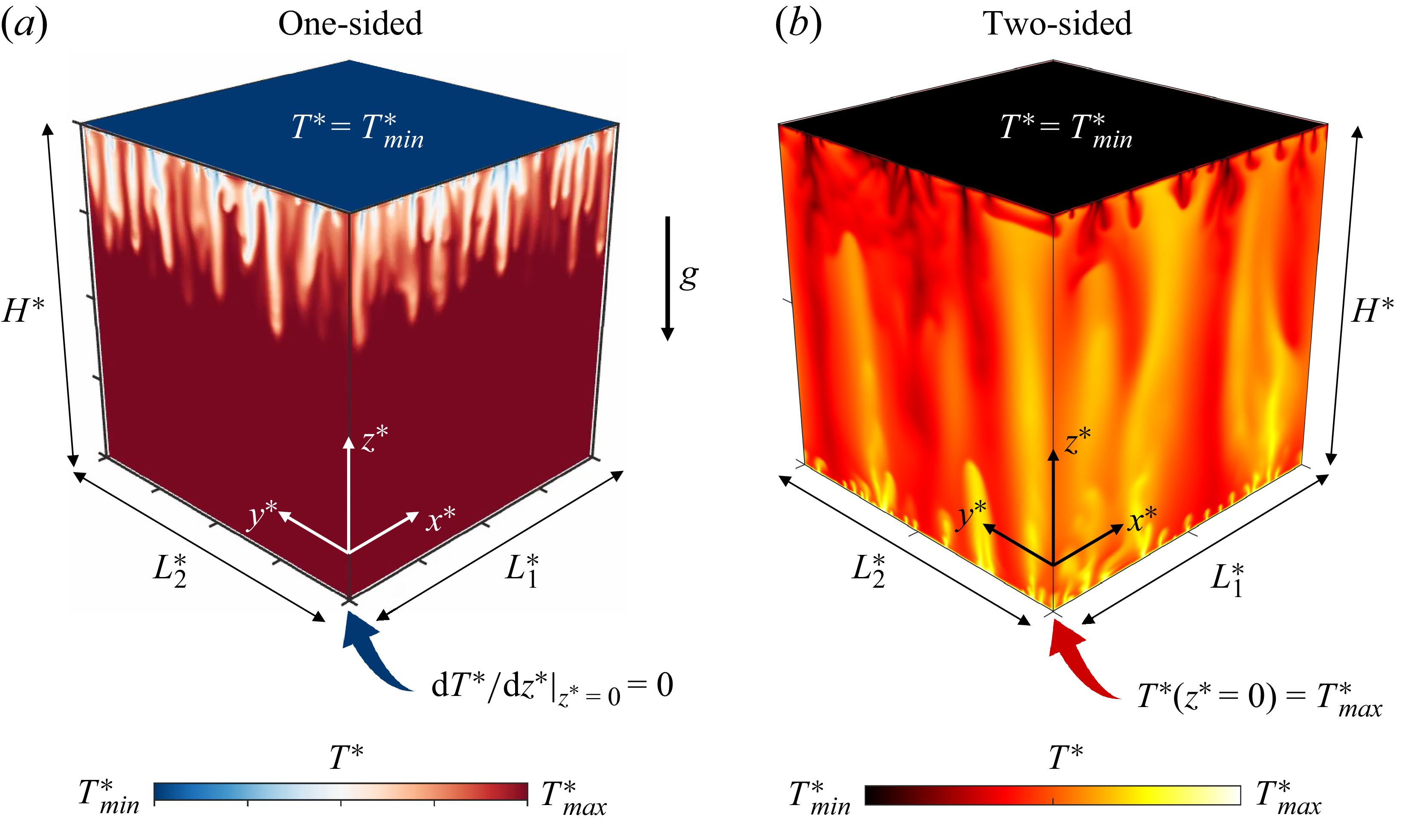
 L1∗,L2∗,H∗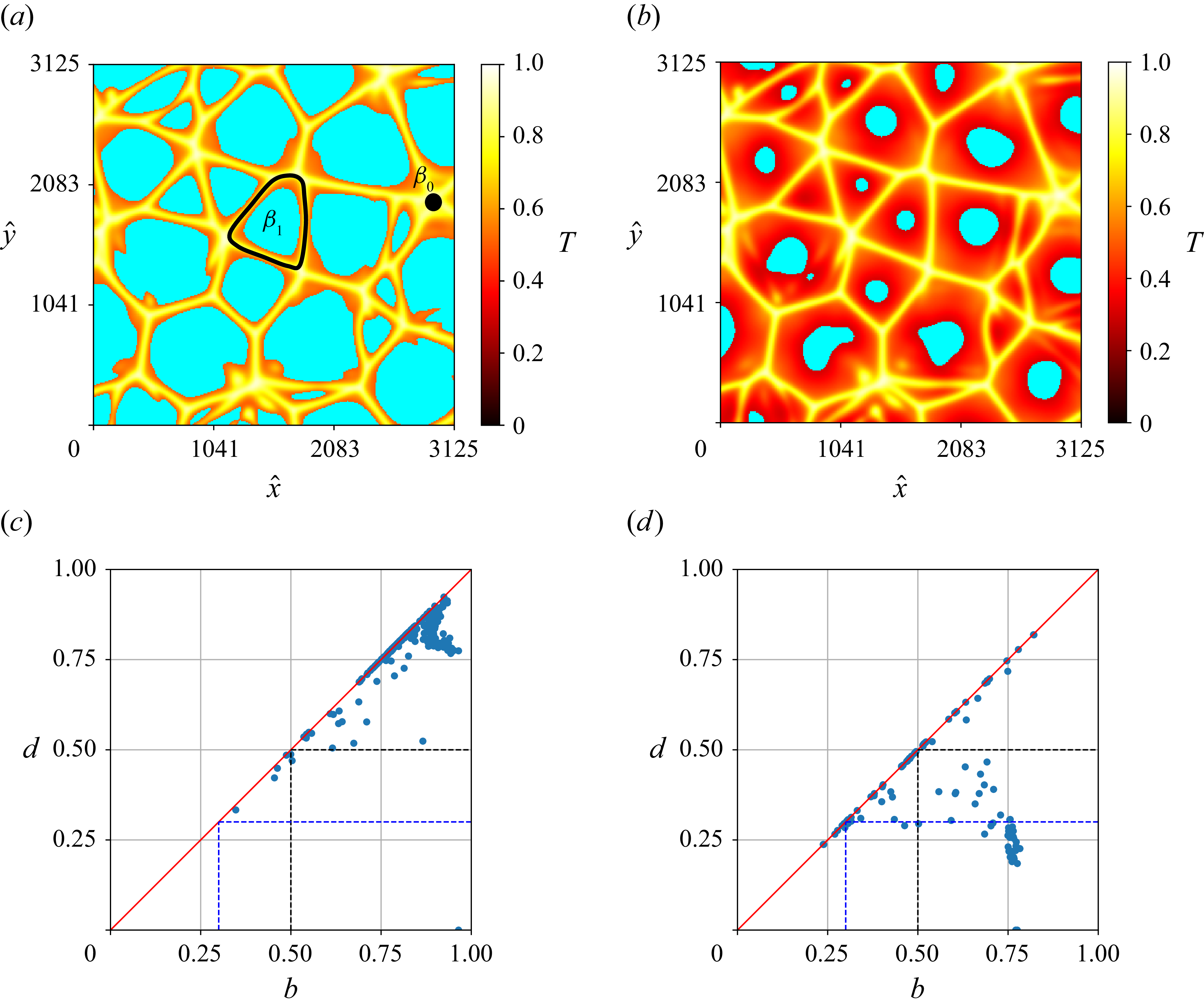
 PD
PD x
x y
y T=0.5
T=0.5 T=0.3
T=0.3 T
T β0
β0 β1
β1 T=0.5
T=0.5 T=0.3
T=0.3 PD
PD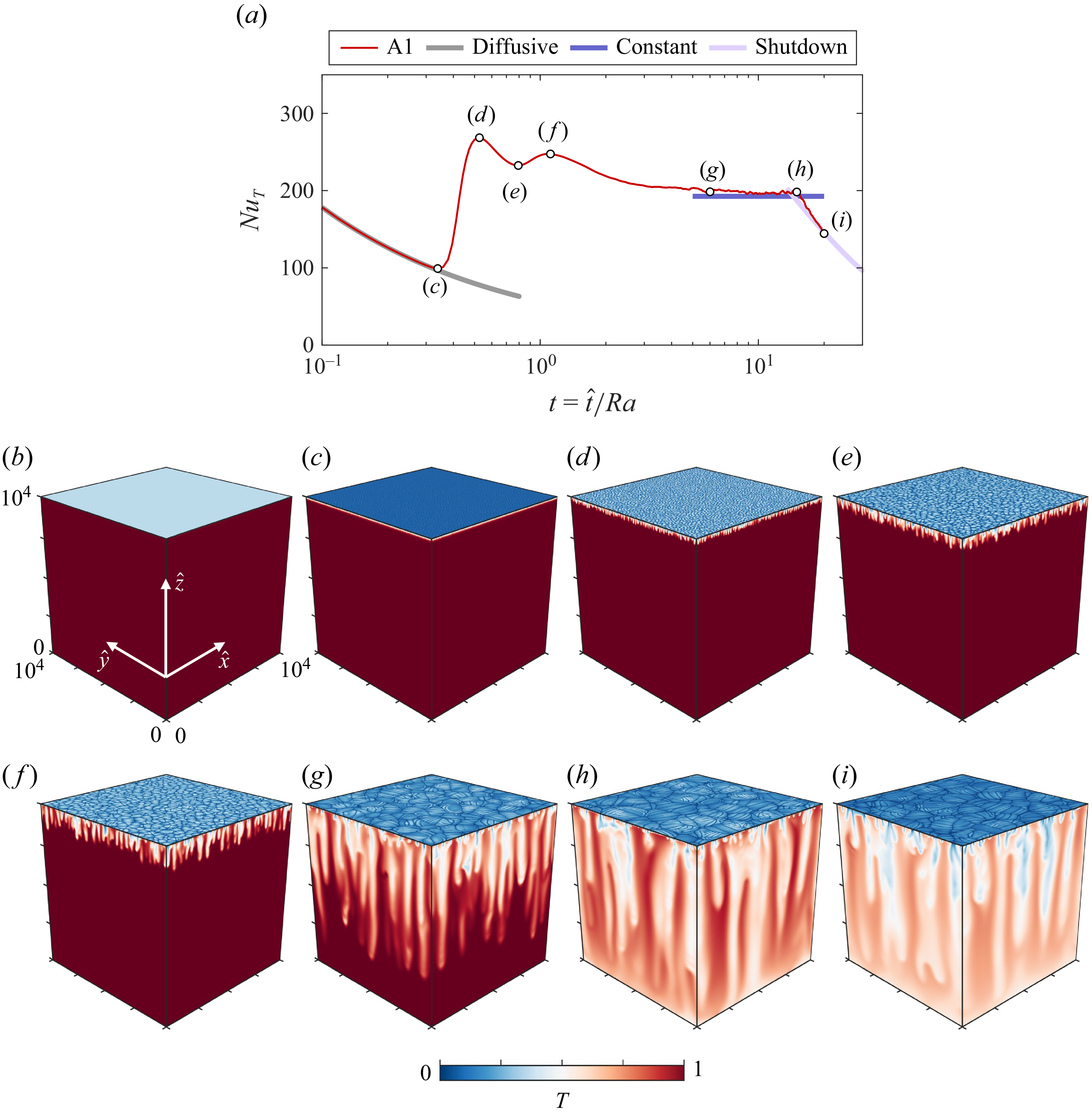
 NuT
NuT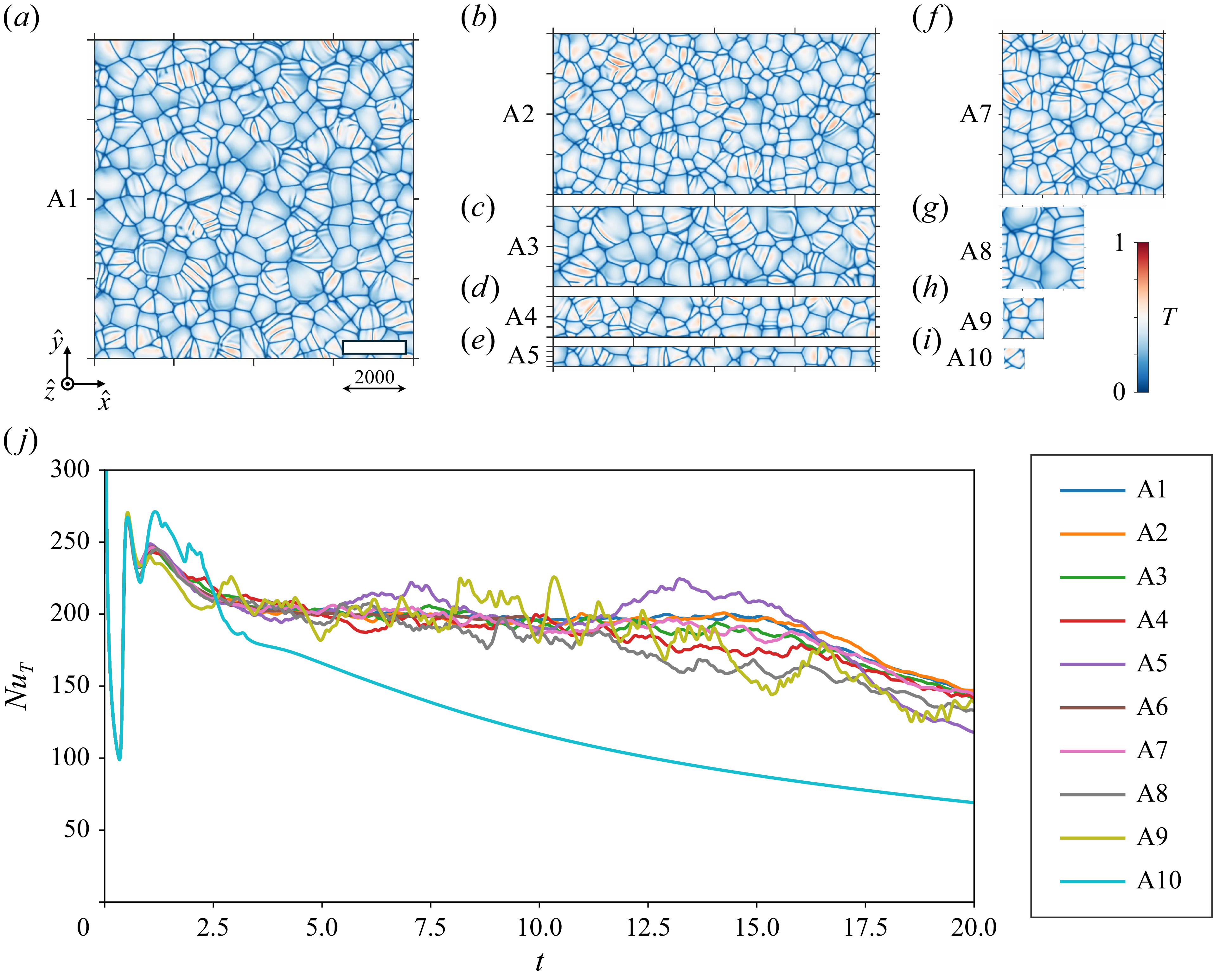
 z=0.998
 t≈0.8
t≈0.8 NuT
NuT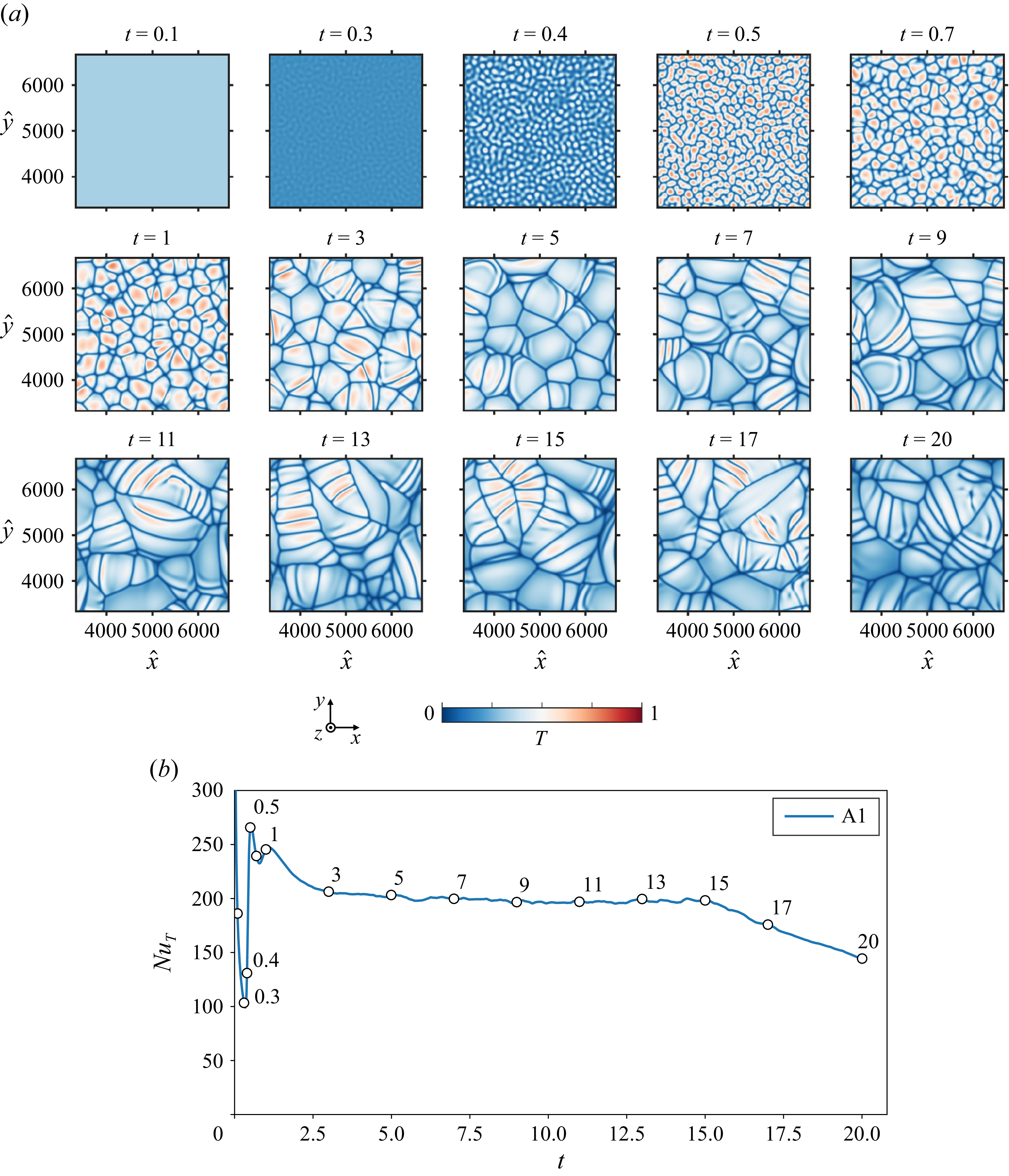
 L^1⩽x,y⩽2L^1/3
 NuT
NuT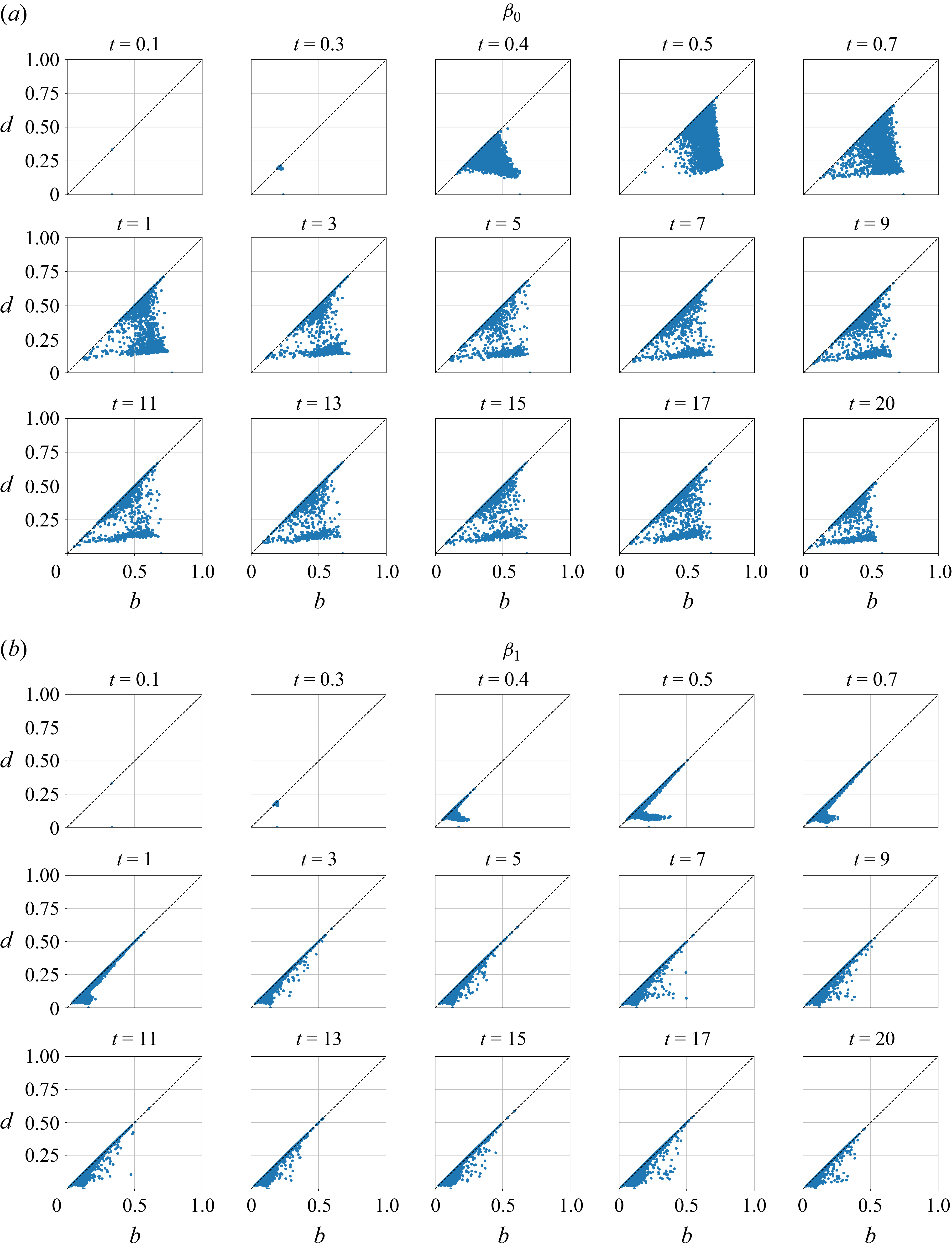
 PD
PD β0
β0 β1
β1 b
b d
d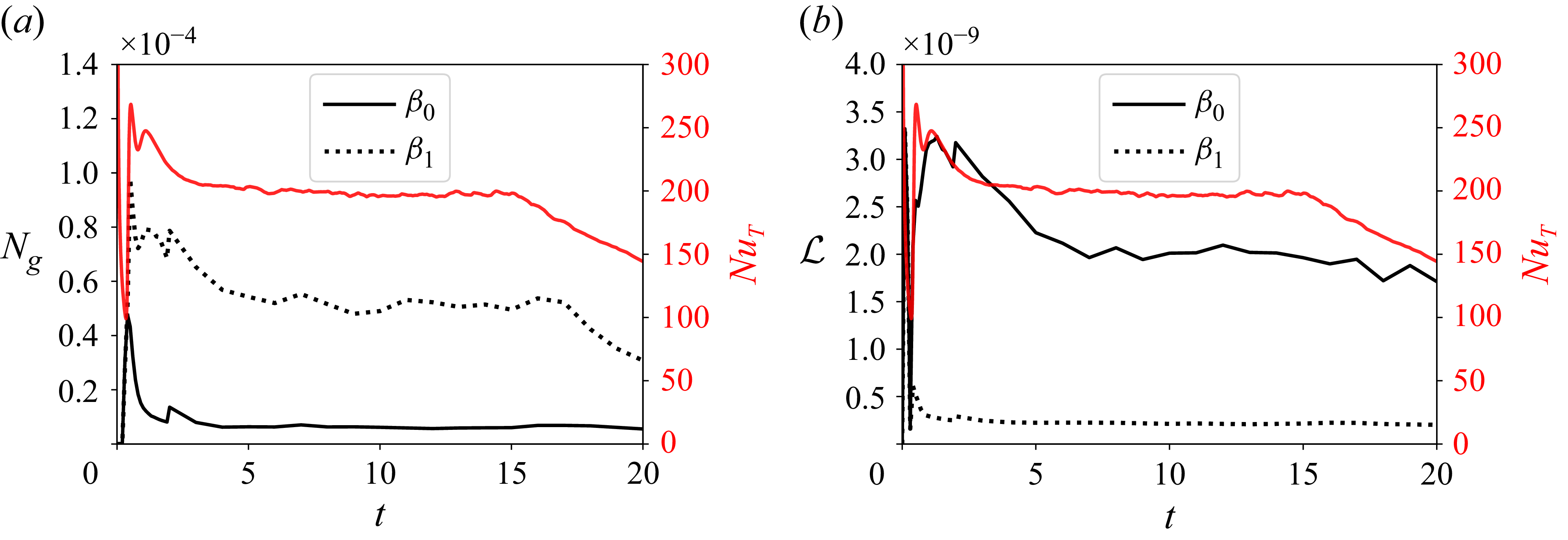
 L^1×L^2
 Ng
Ng L
L β0
β0 β1
β1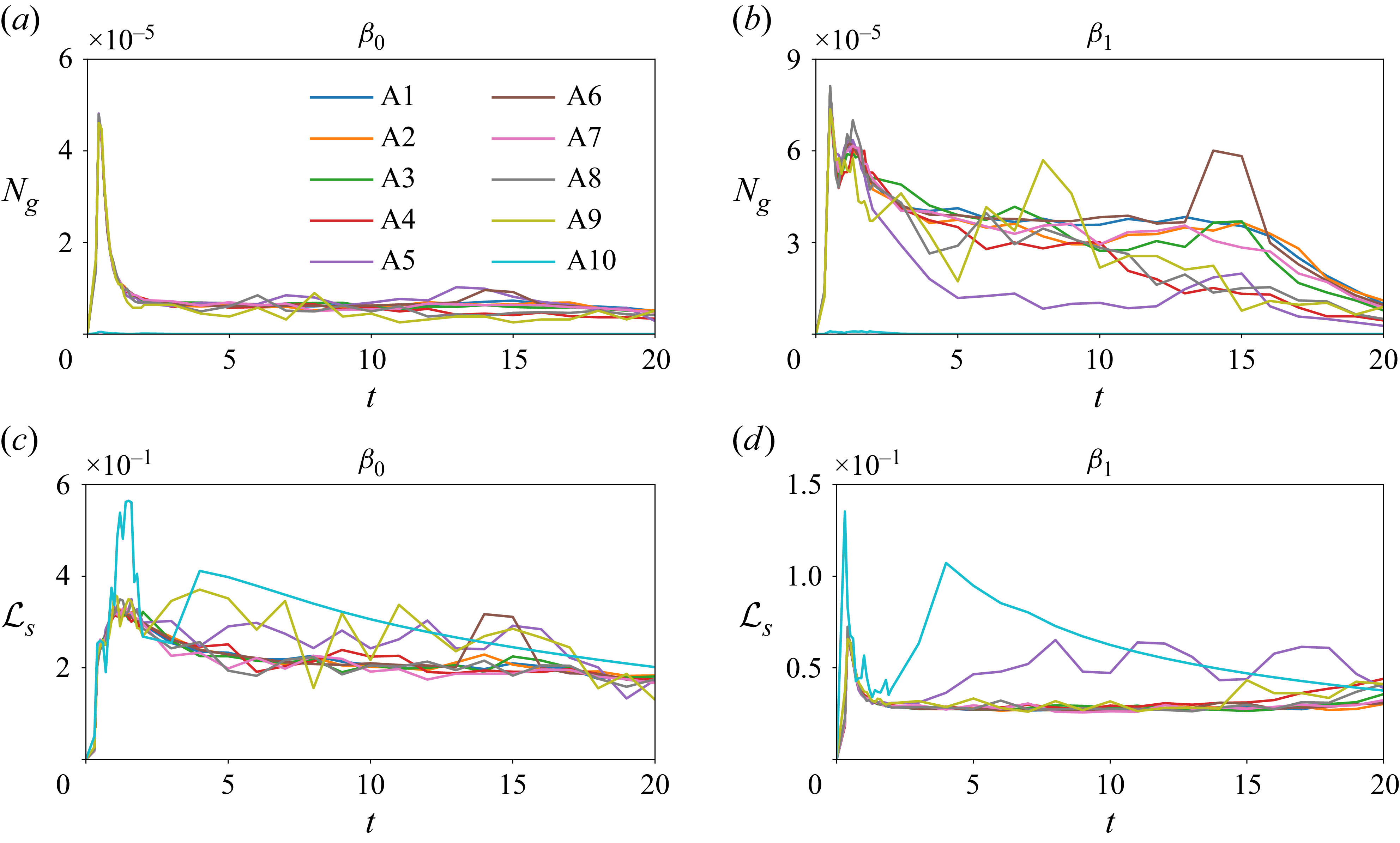
 Ng
Ng L
L β0
β0 β1
β1 Ng
Ng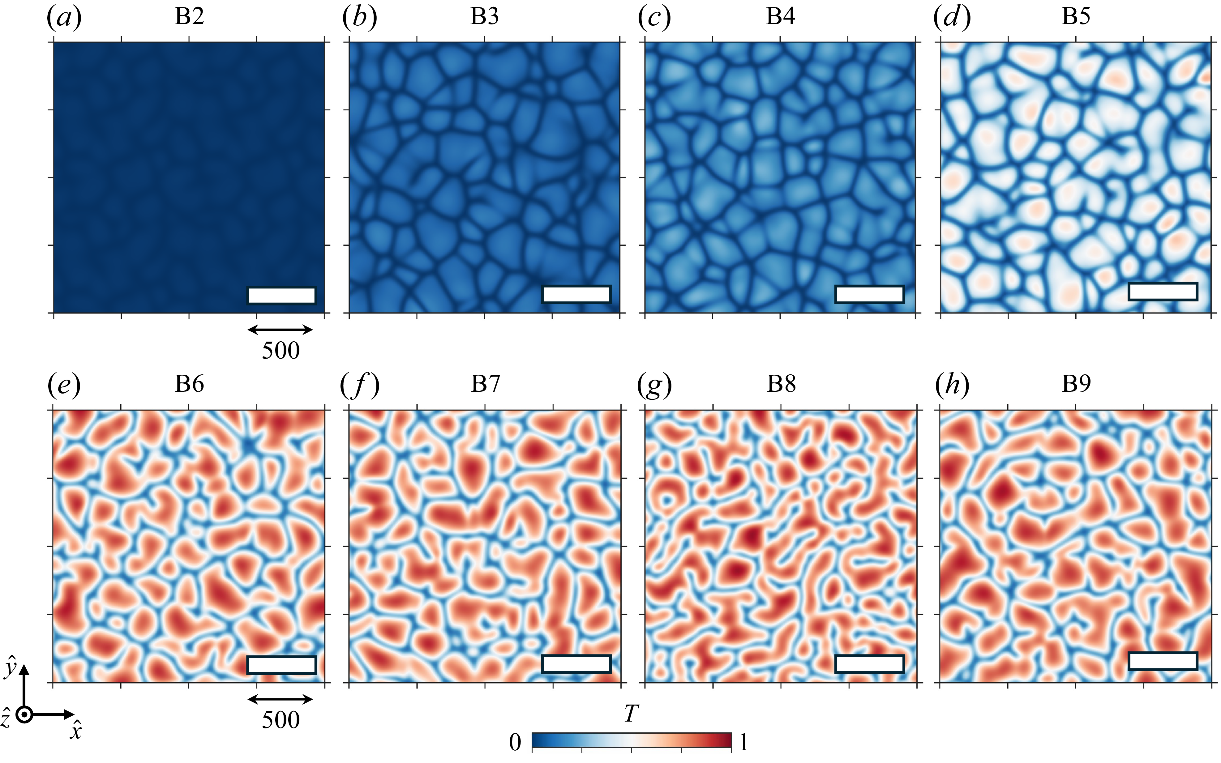
 (x^,y^)
 t^=5×10³
 2×10³
2×10³ 103
103 2×10³
2×10³ 500
500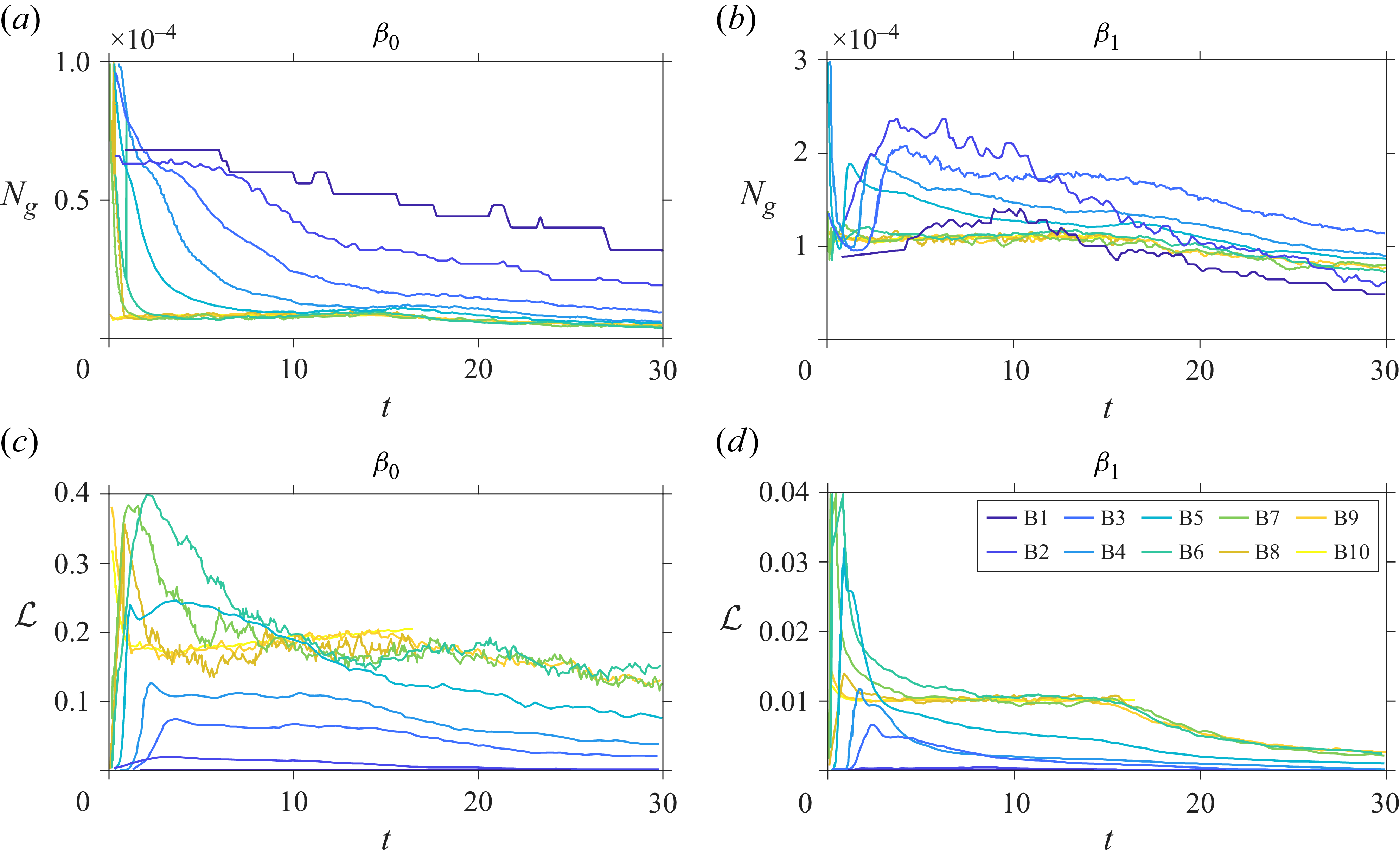
 Ng
Ng L
L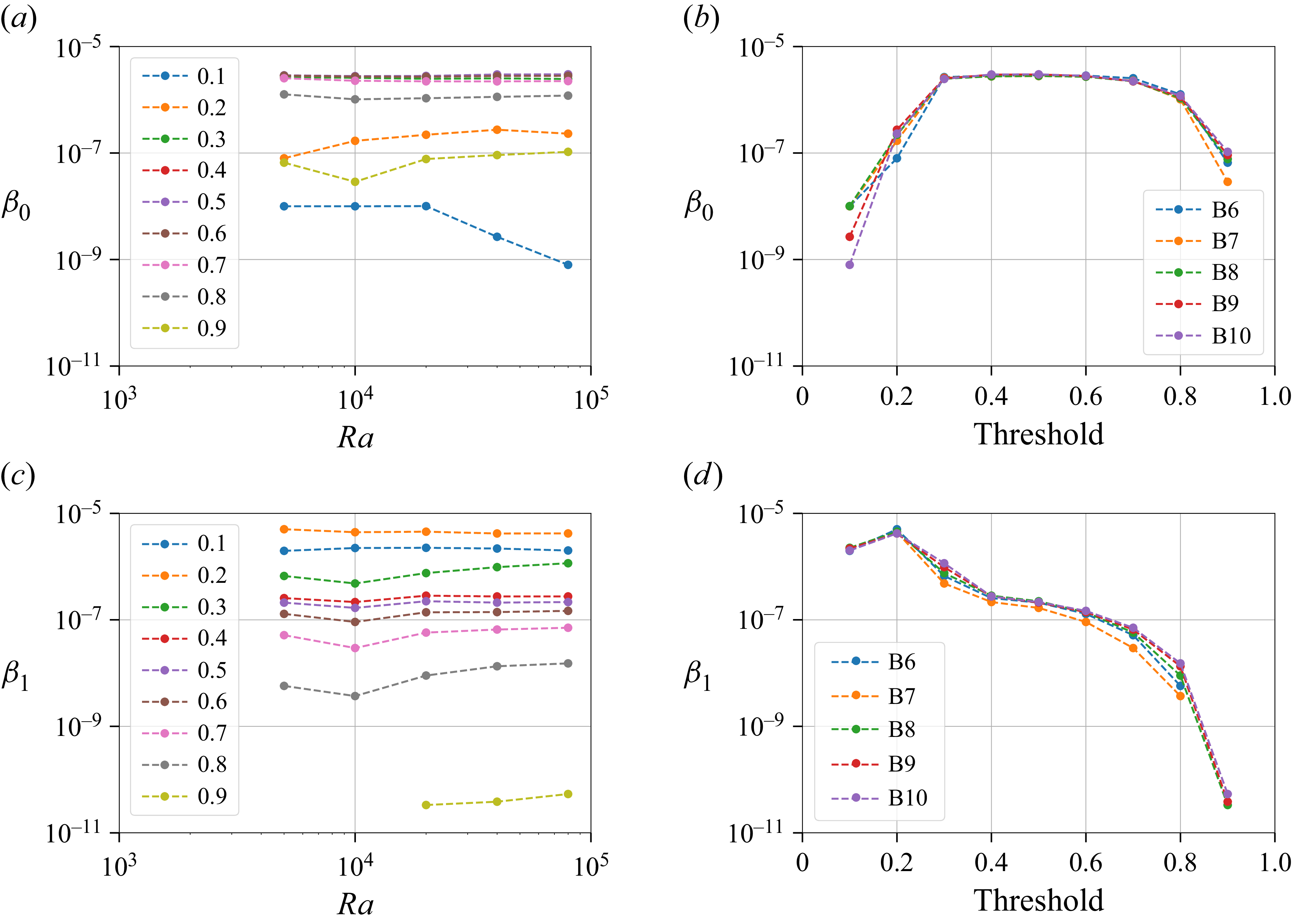
 β0
β0 β1
β1 Ra
Ra Ra
Ra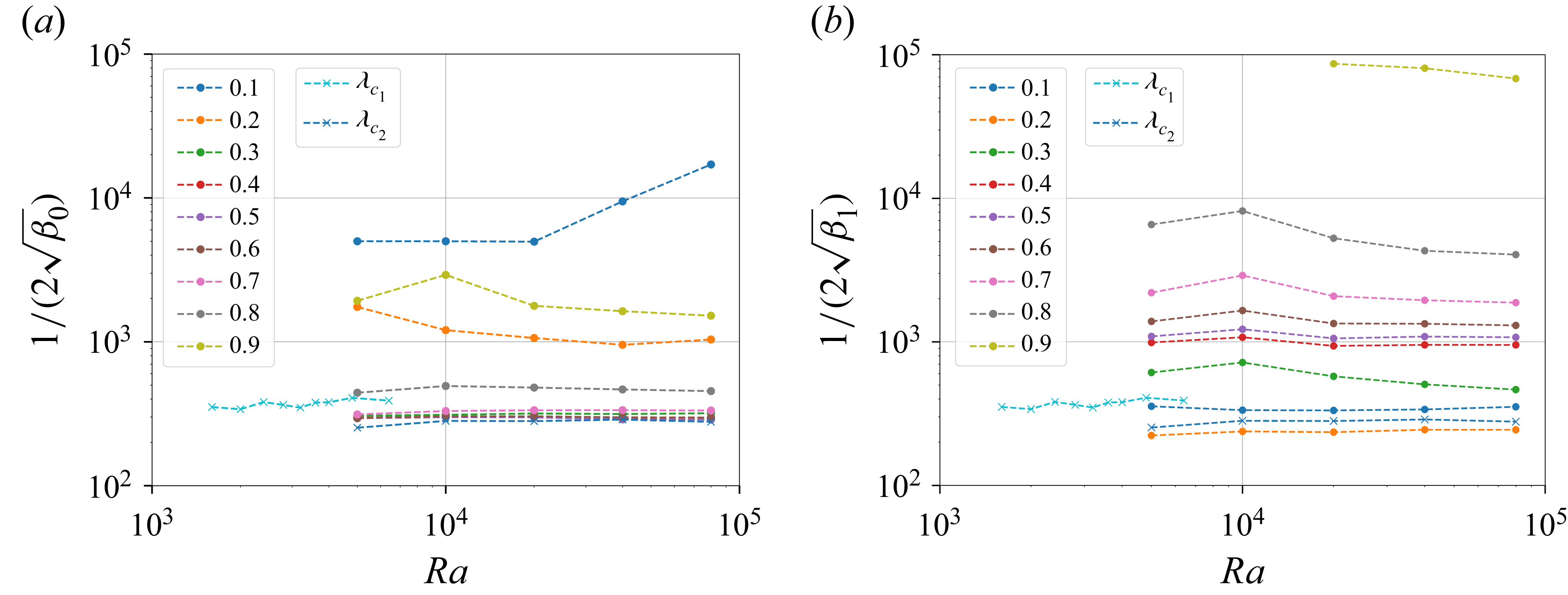
 β0
β0 β1
β1 λc1
λc1 λc2
λc2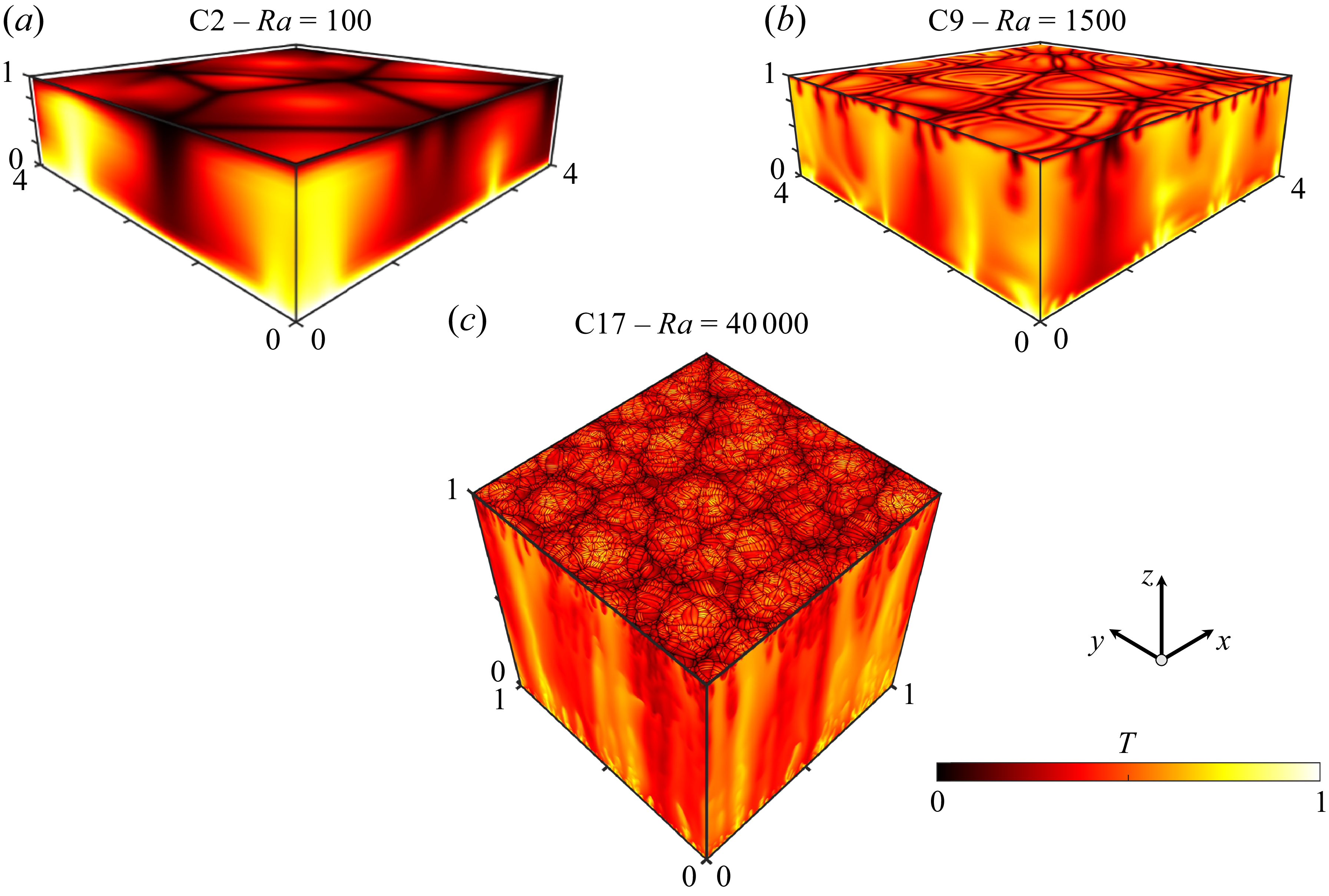
 0⩽x⩽4
0⩽x⩽4 0⩽y⩽4
0⩽y⩽4 0⩽z⩽zt
 0.95⩽zt⩽0.999
 Ra
Ra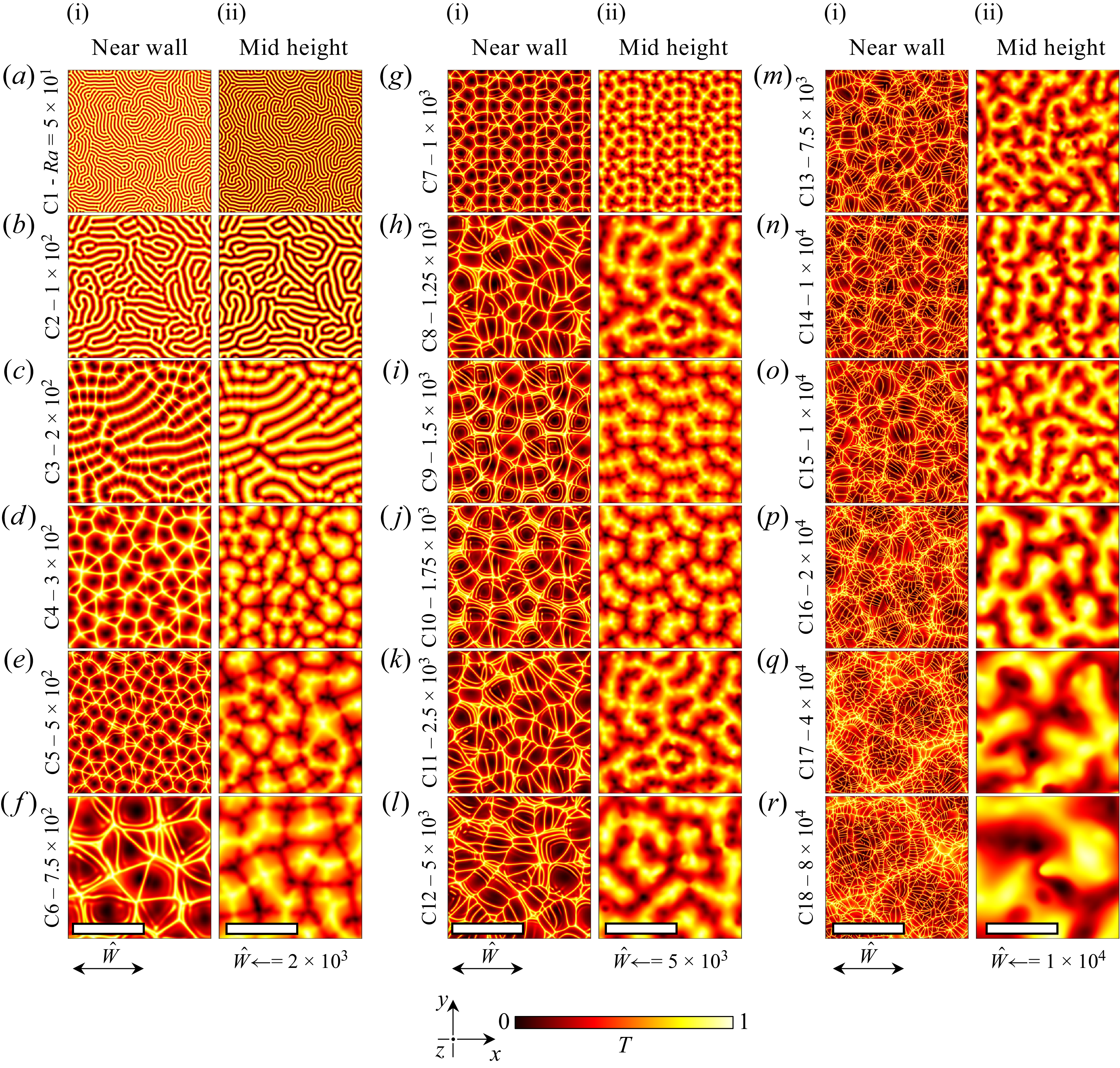
 x,y
x,y z=1/2
z=1/2 Ra
Ra W^
W^ (Ra⩽500)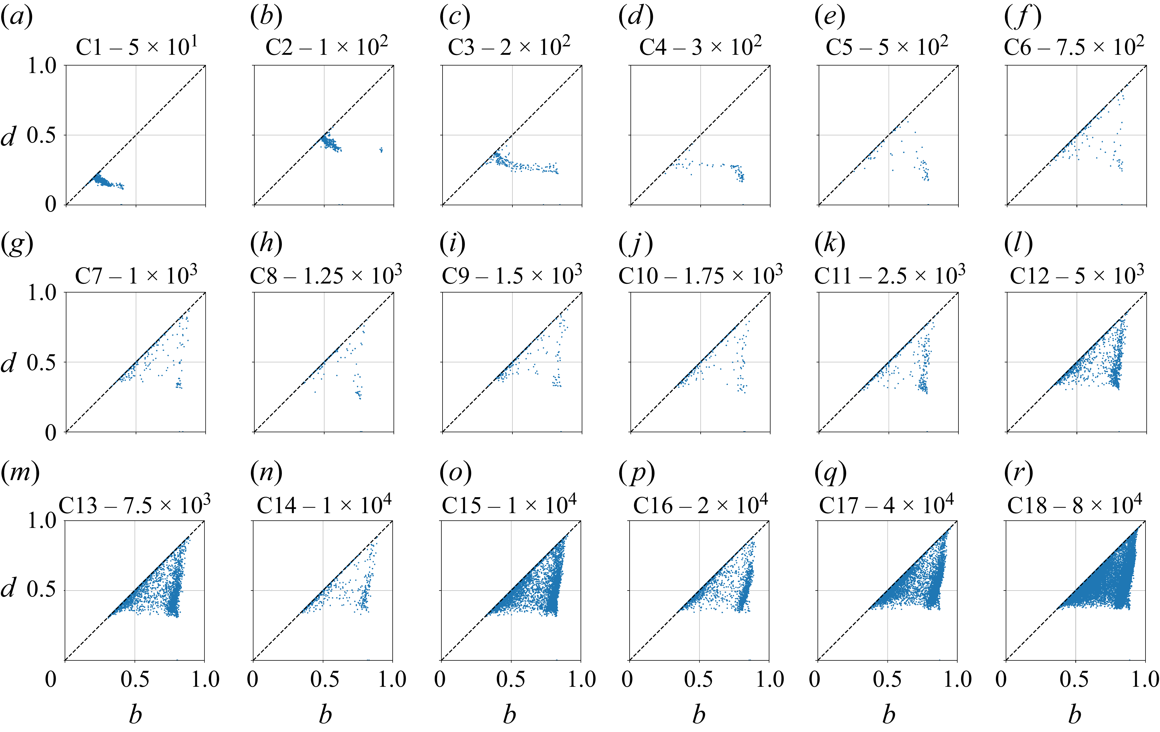
 PD
PD β1PD
β1PD Ra
Ra β1PD
β1PD Ra=300
 Ra=1000
 PD
PD T≈0.75
 Ra⩾2500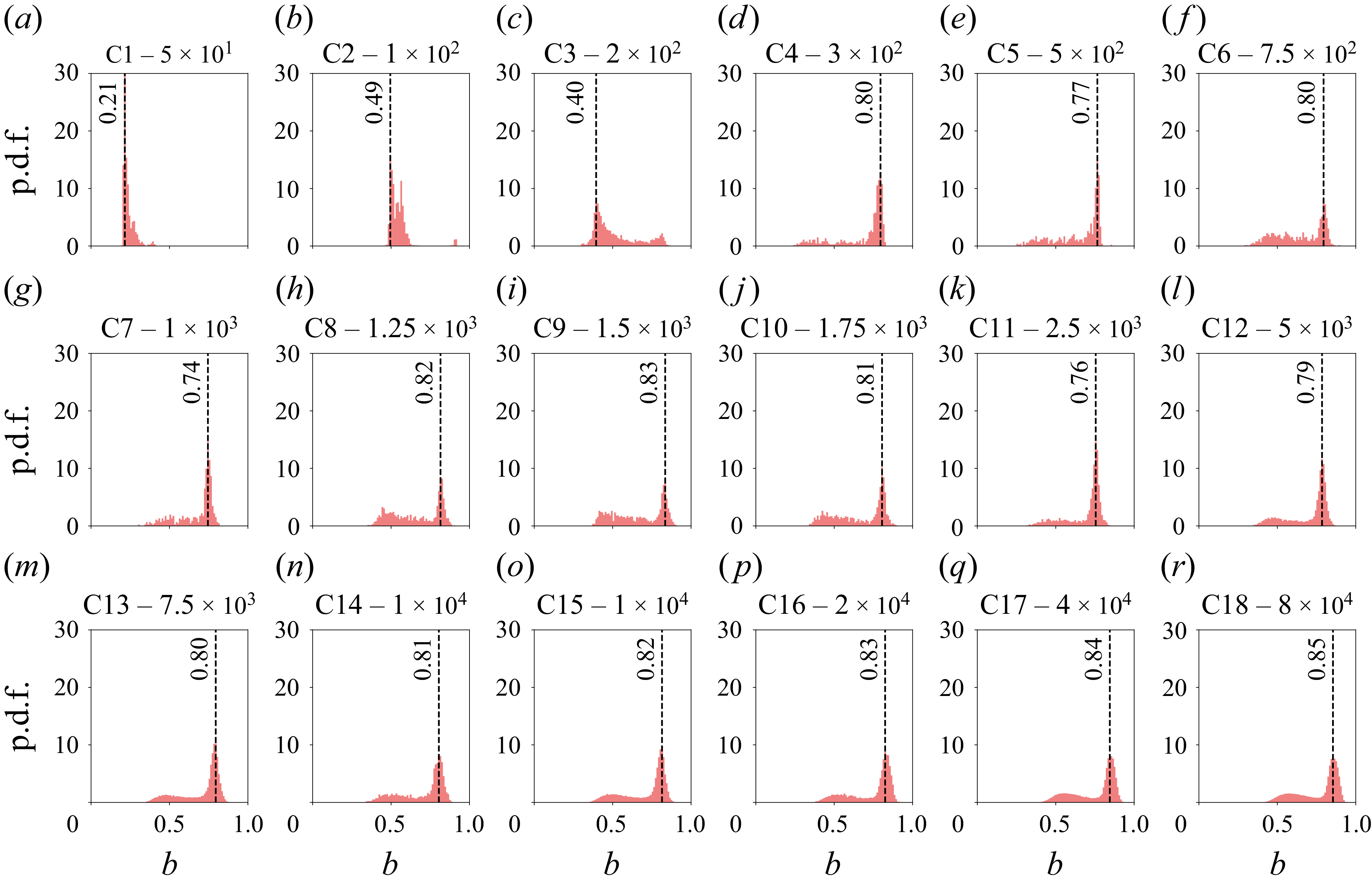
 β1
β1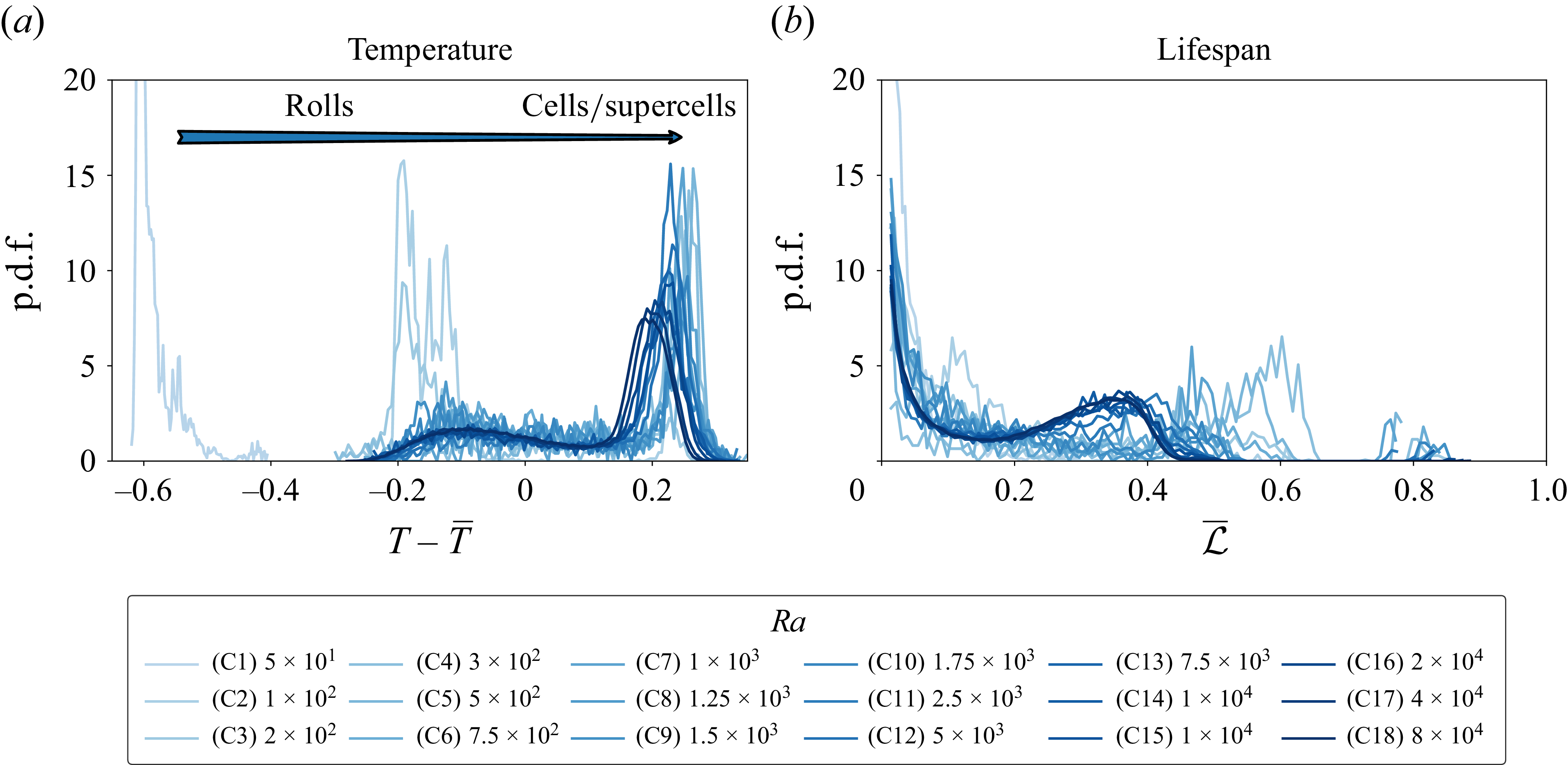
 β1
β1 T¯
T¯ L¯
L¯ Ra
Ra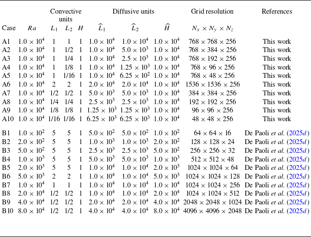
 Ra
Ra L1,L2,H
 L^1,L^2,H^
 Nx×Ny×Nz
 Ra=1×10⁴
 L^1/L^2=L1/L2=1
 Ra
Ra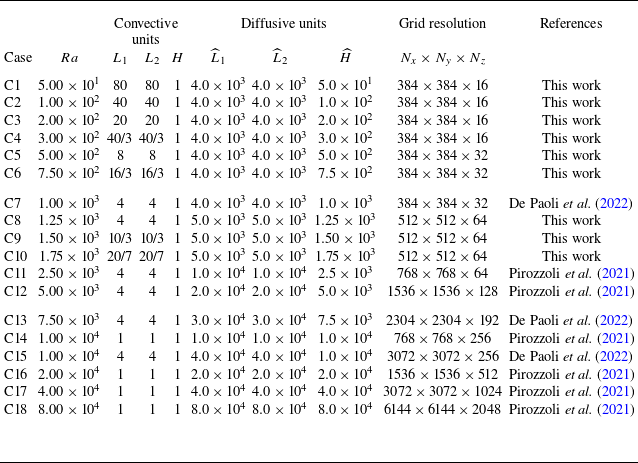
 Ra
Ra H
H L1
L1 L2
L2 H=1,L1=L1∗/H∗,L2=L2∗/H∗
 H^=Ra,L^1=L1∗/ℓ∗
 L^2=L2∗/ℓ∗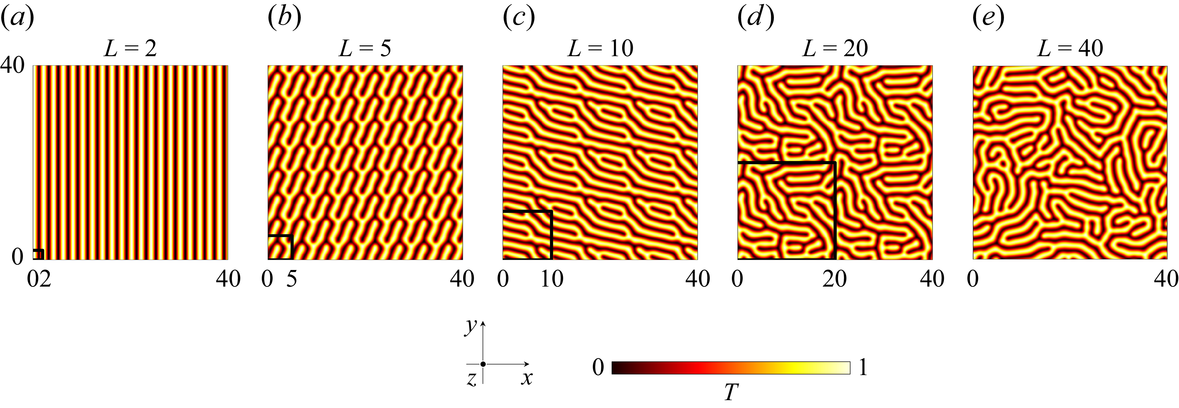
 Ra=102
 L1=L2=L
 L=40
L=40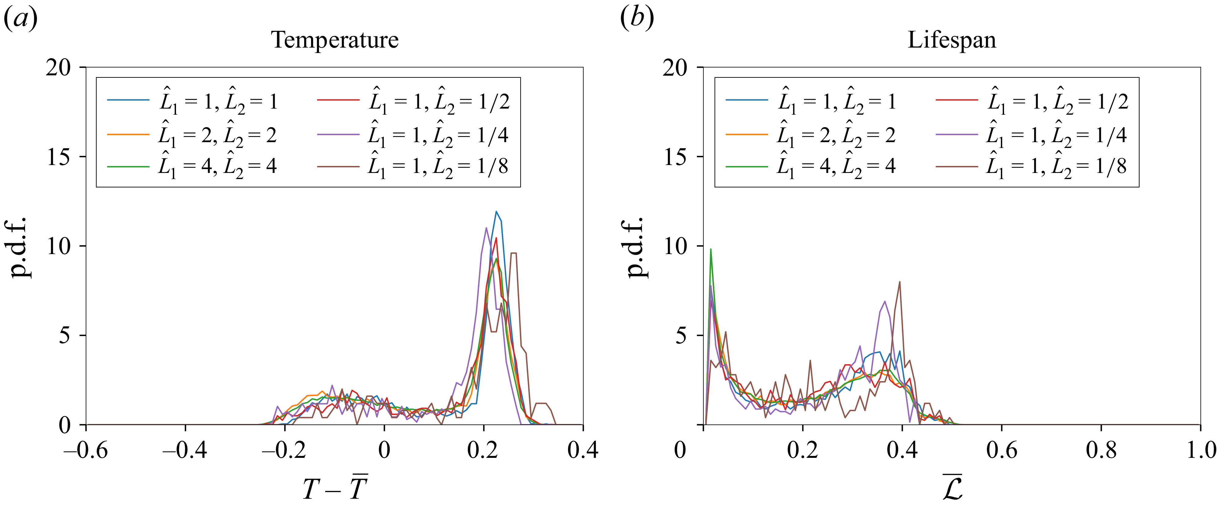
 Ra=104
 β1
β1 T¯
T¯ L¯
L¯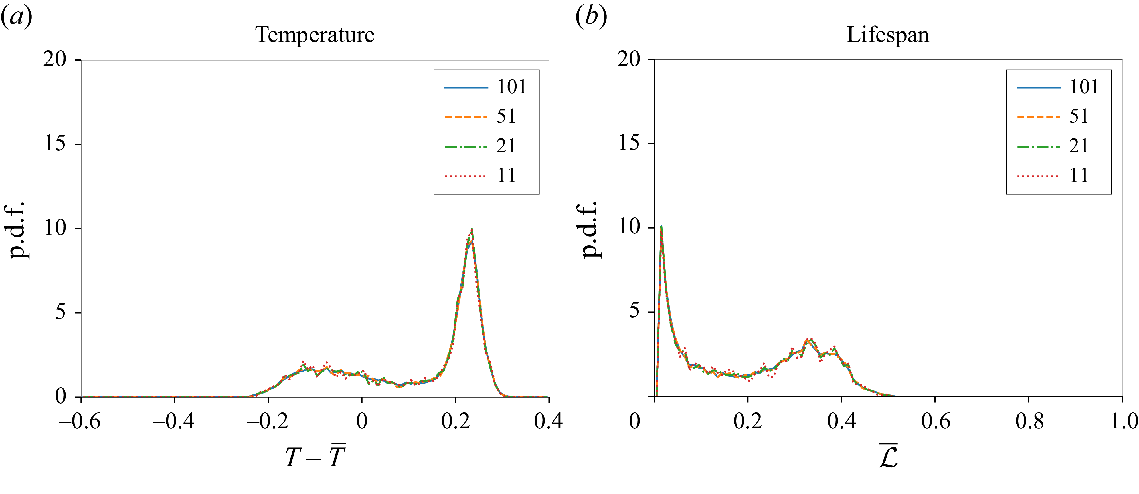
 Ra=104
 β1
β1 T¯
T¯ L¯
L¯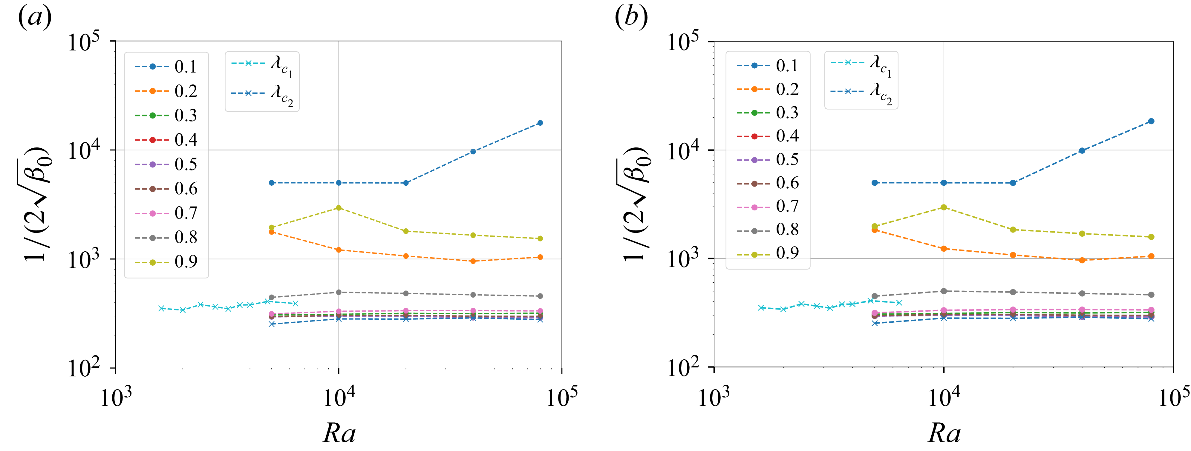


 Open access

