2. Ferrofluid spin-up flow two-phase formulation

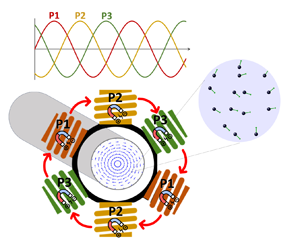
Spin-up flow refers to a macroscopic convective rotational motion elicited in an otherwise quiescent magnetic nanofluid (ferrofluid) by a rotating external magnetic field. To illustrate this process, a suspension of magnetic nanoparticles in a Newtonian liquid is confined in a cylindrical enclosure (radius $R$, length $L$) and subjected to a uniform external magnetic field (frequency $f_0$, intensity $H_0$) applied perpendicular to the $z$-axis of the tube (figure 1a). The magnetic inclusions in the suspension have the unique ability to ‘bodily’ align their permanent magnetic moment vector with the constantly moving magnetic field. Hydrodynamic interaction with the surrounding liquid prevents the discrete magnetic inclusions from achieving perfect alignment with the magnetic field. It is this misalignment, measured as a lag angle, that causes the magnetic inclusions to experience a driving torque at the origin of the macroscopic flow (figure 1b).

Figure 1. Schematic of a ferrofluid spin-up flow geometry in a cylindrical enclosure (a) and a zoomed-in view of a single magnetic nanoparticle (b) subjected to a magnetic field. Here $\boldsymbol {m}$ refers to the orientation of the magnetization vector $\boldsymbol {M}$. Spin-up flow is generated by rotating an external constant modulus magnetic field perpendicular to the axis of symmetry of the cylindrical cell containing the ferrofluid (see (5.1)).

In contrast to the standard ferrohydrodynamic model (Zaitsev & Shliomis Reference Zaitsev and Shliomis1969; Rosensweig Reference Rosensweig2013), which cannot predict spin-up flows (Finlayson Reference Finlayson2013; Torres-Diaz et al. Reference Torres-Diaz, Cortes, Cedeno-Mattei, Perales-Perez and Rinaldi2014; Shliomis Reference Shliomis2021), a comprehensive theoretical representation must account for the two-phase nature of the magnetic suspension. At the very least, this perspective must necessarily include the resolution of the linear and angular momentum equations corresponding to each of the two phases of the magnetic suspension. We propose to tackle the problem by appealing to the AVT, which has been extensively used to describe transport phenomena in two-phase flows and in porous media in particular (Gray Reference Gray1975; Whitaker Reference Whitaker1999; Drew & Passman Reference Drew and Passman2006). The AVT approach models transport phenomena separately in each phase using volume-averaged equations, which are then coupled by jump conditions at interfaces. This makes it possible to analyse the linear and angular momentum transport under the proper distribution of the induced magnetic field within each of the suspension's phases. A notable practical advantage of this method is that it provides average values for unknowns, such as the linear and angular velocities of the magnetic (discrete) phase at each point in the ferrofluid domain. While a macroscopic two-phase description may suffice for non-colloidal suspensions, colloidal ferrofluid particles require the incorporation of Brownian motion into the transport processes, leading to a probabilistic treatment. This coupling can be achieved using the Smoluchowski equation, focusing on its zeroth- and first-order moments, which take into account hydrodynamic conditions and the effect of Brownian motion on the average transport of particles and the orientation of their magnetic moments. Section 4 will go over the connection of the two-phase ferrofluid model with the zeroth- and first-order moments of the Smoluchowski equation.

Consider a two-phase suspension consisting of a liquid, denoted by the subscript ${l}$, and a dispersed magnetic phase (particles), denoted by the subscript ${p}$. Figure 2 is a schematic representation of the ferrofluid system parsed into representative elementary volumes (REV), over which the transport equations of the two phases are averaged. Such two phases (${l}$ and ${p}$) occupy the volumes $V_{l},V_{p}$, respectively, in the REV volume $V$, whose perimeter is bounded by the surface $\varGamma =A_{p-e} \cup A_{{l}-{e}}$. The interface separating the two phases inside the REV is denoted by $A_{{l}-{p}}$ with the normal orientational unit vectors $\boldsymbol {n}_{l}=-\boldsymbol {n}_{p}$. Let $\boldsymbol {x}$ be the macroscopic position vector characterizing the centre of the elementary volume with respect to the macroscopic system, and $\boldsymbol {y}$ the microscopic position vector on the scale of the REV, defined with respect to its centroid. For example, consider a scalar field $\varPhi _{l}$ transported in phase $\rm {l}$, defined with respect to position $\boldsymbol {x}+\boldsymbol {y}$. Using AVT, the mean field $\langle \varPhi _{l} \rangle$ with respect to REV is given by (Gray Reference Gray1975; Whitaker Reference Whitaker1999)

(2.1)\begin{equation} \langle \varPhi_{l}\rangle|_{\boldsymbol{x}} = \frac{1}{V} \int_V \chi_{l} \varPhi_{l}|_{\boldsymbol{x}+\boldsymbol{y}}\,{\rm d} V, \end{equation}

where $\chi _{l}$ denotes the phase indicator describing the spatial distribution of phase ${l}$ in the REV. The latter is defined by

(2.2)\begin{equation} \left. \begin{array}{ll@{}} \chi_{l} = 1 & \boldsymbol{x}+\boldsymbol{y} \in V_{l} \cup A_{{l}-{p}}, \\ 0 & \text{elsewhere}. \end{array} \right\} \end{equation}

Figure 2. Schematic description of a REV of a suspension composed of a liquid and rigid spherical particles.

Supplementary materials (§ 1) available at https://doi.org/10.1017/jfm.2024.32 contain the developments according to the AVT approach leading to the formulation of the mean transport equation for the so-called quantity $\varPhi _{l}$.

2.1. Ferrofluid phase-specific microscale transport equations

To establish average macroscopic transport equations governing the ferrofluid behaviour at each macroscopic position $\boldsymbol{x}$ within the REV, one must first formulate microscopic transport equations for the two suspension phases at each microscopic position $\boldsymbol{y}$ within the REV. These equations involve the conservation of mass, linear and angular momentum and the application of Maxwell's equations to describe the magnetic fields in each ferrofluid phase.

The microscale equation of the incompressible liquid phase (2.3) represents the mass conservation equation of the liquid as a continuum:

(2.3)\begin{equation} \boldsymbol{\nabla} \boldsymbol{\cdot} (\chi_{l} \boldsymbol{v}_{l}) = 0. \end{equation}

While the liquid phase at the microscale (represented by points $\boldsymbol {y}$ in figure 2) can be described as a continuum using a microscopic mass conservation equation (see (2.3)), this approach does not hold for the discrete magnetic phase. To address this, we establish mass conservation for individual particles within the REV by relying on the mass invariance of a single particle. Specifically, we relate the mass of an individual particle (i) to its density $\rho _{p}$, particle volume $V_{p}$ and phase indicator $\chi ^i_{p}$:

(2.4)\begin{equation} m^i_{p} = \int_{V_{p}} \rho_{p}\,{\rm d} V = \chi_{p}^i \rho_{p} V_{p}, \end{equation}

where $V_{p}$ is the volume of a single particle.

Assuming constant physicochemical properties, the linear momentum conservation equation for the liquid phase at the microscopic scale is

(2.5)\begin{equation} \rho_{l} \left(\frac{\partial \chi_{l} \boldsymbol{v}_{l}}{\partial t} + \boldsymbol{\nabla} \boldsymbol{\cdot} (\chi_{l} \boldsymbol{v}_{l} \otimes \boldsymbol{v}_{l})\right) = \boldsymbol{\nabla} \boldsymbol{\cdot} {\boldsymbol{\mathcal{T}}}_{\!l} + \boldsymbol{F}^{e}_{l}, \end{equation}

where ${\boldsymbol{\mathcal{T}}}_{\!l}$ is the viscous-pressure stress tensor containing the symmetric part characterizing shear stress. The term $\boldsymbol {F}^{e}_{l}$ refers to an external volume force.

For a Newtonian and non-polar liquid, the stress tensor, ${\boldsymbol{\mathcal{T}}}_{\!l}$, is given by the following relation:

(2.6)\begin{equation} {\boldsymbol{\mathcal{T}}}_{\!l} =-\chi_{l} P \boldsymbol{\mathsf{I}}+ \mu ({\boldsymbol{\nabla}} \chi_{l} \boldsymbol{v}_{l} + ({\boldsymbol{\nabla}} \chi_{l} \boldsymbol{v}_{l})^{t} -\tfrac{2}{3} \boldsymbol{\nabla} \boldsymbol{\cdot} (\chi_{l} \boldsymbol{v}_{l}) \boldsymbol{\mathsf{I}}) +\mu_b \boldsymbol{\nabla} \boldsymbol{\cdot} (\chi_{l} \boldsymbol{v}_{l}) \boldsymbol{\mathsf{I}}, \end{equation}

where the dynamic viscosity, $\mu$, of the liquid is assumed constant. $\mu _{b}$ is the bulk viscosity associated with expansion (compression) processes.

Taking into account that the bulk viscosity, $\mu _b$, is often negligible in the case of fluids, and based on the liquid continuity (2.3) which describes the incompressibility of the fluid with zero divergence of the velocity field, the stress tensor (2.6), reduces to

(2.7)\begin{equation} {\boldsymbol{\mathcal{T}}}_{\!l} =-\chi_{l} P \boldsymbol{\mathsf{I}}+ \mu ({\boldsymbol{\nabla}} \chi_{l} \boldsymbol{v}_{l} + ({\boldsymbol{\nabla}} \chi_{l} \boldsymbol{v}_{l})^{t}). \end{equation}

By substituting (2.7) in (2.5), the liquid's linear momentum equation becomes

(2.8)\begin{equation} \rho_{l} \left(\frac{\partial \chi_{l} \boldsymbol{v}_{l}}{\partial t} + \boldsymbol{\nabla} \boldsymbol{\cdot} (\chi_{l} \boldsymbol{v}_{l} \otimes \boldsymbol{v}_{l} )\right) =-\boldsymbol{\nabla} \chi_l P + \mu \boldsymbol{\nabla}\boldsymbol{\cdot} {\boldsymbol{\nabla}} \chi_l \boldsymbol{v}_l + \boldsymbol{F}^{e}_{l}. \end{equation}

It is important to emphasize that at the microscopic scale within the REV, where the particles are individually spaced and do not form a continuous medium, the equation governing the angular momentum of the particles does not have a conventional continuum relationship. Therefore, the force balance on a single particle $i$ is used as a microscopic equation as a prerequisite to derive a macroscopic continuum equation for all particles in the REV. The momentum conservation equation for a Brownian particle $i$, also known as the Langevin equation, is expressed as follows:

(2.9)\begin{equation} \rho_{p} \left.\frac{{\rm d} \boldsymbol{v}_{p}^i}{{\rm d} t}\right|_{\boldsymbol{y}=\boldsymbol{y}_i} = \boldsymbol{F}_i^{lp} + \boldsymbol{F}_i^{pp} + \boldsymbol{F}_i^{e}, \end{equation}

where $\boldsymbol {v}_{p}^i(\kern0.7pt \boldsymbol {y}_i)$ is the velocity of the particle $i$ evaluated at its centre of mass $\boldsymbol {y}=\boldsymbol {y}_i$. Here $\boldsymbol {F}_i$ denotes an external force per unit volume. The subscripts $lp,pp$ refer to the liquid–particle and particle–particle interaction forces, respectively.

The conservation equation of angular momentum at the microscopic scale is modelled similarly to the conservation equations of mass and linear momentum of particles by the angular Langevin equation of a particle $i$,

(2.10)\begin{equation} I_{p} \left.\frac{{\rm d} \boldsymbol{w}_{p}^i}{{\rm d} t}\right |_{\boldsymbol{y}=\boldsymbol{y}_i} = \boldsymbol{\varGamma}_i^{lp} + \boldsymbol{\varGamma}_i^{pp} + \boldsymbol{\varGamma}_i^{e}, \end{equation}

where $\boldsymbol {w}_{p}^i(\kern0.7pt \boldsymbol {y}_i)$ is the angular velocity of the particle $i$ evaluated at $\boldsymbol {y}=\boldsymbol {y}_i$; $I_{p}= \frac {2}{5} \rho _{p} R_{p}^2$ is the moment of inertia of the particle $i$ per unit volume of a particle; $\boldsymbol {\varGamma }_i$ denotes the force moment per unit volume of the particle $i$; $\boldsymbol {\varGamma }_i^{e}$ denotes the external moment, per unit volume, exerted on the particle $i$; and $\boldsymbol {\varGamma }_i^{lp}$ and $\boldsymbol {\varGamma }_i^{pp}$ are the force moments of liquid–particle and particle–particle interactions, respectively.

When an external magnetic field is applied to a ferromagnetic suspension, an induced magnetic field is created within its constitutive liquid and nanoparticle phases. While this induced field affects both phases, the magnetization process itself, which involves the alignment magnetic moments, is exclusive to the ferromagnetic particles. Thus, a magnetic torque is exerted only on the nanoparticles. Consequently, the microscopic modelling of the angular momentum considers only the discrete magnetic phase while explicit modelling of the liquid angular momentum is unnecessary. Assuming that the ferrofluid consists of non-conducting discrete magnetic inclusions and a liquid, Maxwell's equations can be simplified to Maxwell–Ampère and Maxwell-flux equations without charge displacement or electric current. At the microscopic level, the Maxwell–Ampère equations for ${l}$ and ${p}$ are as follows:

(2.11)$$\begin{gather} \boldsymbol{\nabla} \times (\chi_{l} \boldsymbol{H}_{l}) = 0 \quad \in V_{l}, \end{gather}$$

(2.12)$$\begin{gather}\boldsymbol{\nabla} \times (\chi_{p} \boldsymbol{H}_{p}) = 0 \quad \in V_{p}, \end{gather}$$

where $\boldsymbol {H}$ is the magnetic field vector expressed in ${A/m}$ and $\mu _0= 4 \times {\rm \pi}10^{-7}\ {\rm N}/{\rm A}^{-2}$ is the vacuum magnetic permeability.

While the Maxwell-flux equations of ${l}$ and ${p}$ read as follows:

(2.13)$$\begin{gather} \boldsymbol{\nabla} \boldsymbol{\cdot} (\chi_{l} \boldsymbol{B}_{l}) = 0 \quad \in V_{l}, \end{gather}$$

(2.14)$$\begin{gather}\boldsymbol{\nabla} \boldsymbol{\cdot} (\chi_{p} \boldsymbol{B}_{p}) = 0 \quad \in V_{p}, \end{gather}$$

where $\boldsymbol {B}$ is the magnetic induction vector which can be formally expressed in terms of the magnetization vector, $\boldsymbol {M}$, by the following relation:

(2.15)\begin{equation} \boldsymbol{B} = \mu_0 (\boldsymbol{H} + \boldsymbol{M}). \end{equation}

Liquids constituting ferrofluids are in general linear, homogeneous and isotropic media, where the magnetization is directly proportional to the magnetic field vector, such as

(2.16)\begin{equation} \boldsymbol{M}_{l} = \varphi \boldsymbol{H}_{l}, \end{equation}

where the dimensionless proportionality constant is called magnetic susceptibility. Liquids are generally weakly magnetized where the value of $\varphi$ is very small. Furthermore, $\varphi$ is positive if the material is paramagnetic and negative if the material is diamagnetic. Using the magnetization expression (2.16), the magnetic induction vector $\boldsymbol {B}_{l}$ in the liquid phase is written as follows:

(2.17)\begin{equation} \boldsymbol{B}_{l} = \mu_0 (1 + \varphi_{l}) \boldsymbol{H}_{l}. \end{equation}

In the case where the liquid is non-magnetic, $|\varphi _{l}| <<1$, the expression for the magnetic induction reduces to

(2.18)\begin{equation} \boldsymbol{B}_{l} = \mu_0 \boldsymbol{H}_{l}. \end{equation}

Compared with the liquid, the particles are superparamagnetic because they are considered monodomain with a permanent magnetic moment $\boldsymbol {M}_{p}=M_{d}\boldsymbol {m}$. The magnetic induction vector of the particles in this case can be written as

(2.19)\begin{equation} \boldsymbol{B}_{p} = \mu_0 (\boldsymbol{H}_{p} + M_{d} \boldsymbol{m}), \end{equation}

where $M_{d}$ refers to the domain magnetization of the particles and $\boldsymbol {m}$ denotes the orientation of particles’ magnetic moments (figure 1b). It should be noted that the model governing the orientation dynamics of the particles’ magnetic moments, $\boldsymbol {m}$, with respect to the magnetic field, $\boldsymbol {H}$, is described in detail in § 4.

Taking into account the expressions of the induction vectors of both phases (2.18), (2.19), the Maxwell-flux equations read as follows:

(2.20)$$\begin{gather} \boldsymbol{\nabla} \boldsymbol{\cdot} (\chi_{l} \boldsymbol{H}_{l}) = 0 \quad \in V_{l}, \end{gather}$$

(2.21)$$\begin{gather}\boldsymbol{\nabla} \boldsymbol{\cdot} \chi_{p} (\boldsymbol{H}_{p} + M_{d} \boldsymbol{m}) = 0 \quad \in V_{p}. \end{gather}$$

2.2. Ferrofluid macroscale two-phase transport equations

To establish the macroscale transport equations for a two-phase ferrofluid, a methodology similar to that used in the supplementary materials (§ 2) to derive the hypothetical scalar field transport equation $\varPhi _{l}$ can be applied. This approach involves averaging each transport equation over the REV and using Gray's decomposition (Gray Reference Gray1975). The derivation of the averaged transport equations is also presented in detail in the supplementary materials.

Applying the AVT to the liquid mass conservation equation at the microscopic scale, (2.3), yields

(2.22)\begin{equation} \boldsymbol{\nabla} \boldsymbol{\cdot} (\epsilon_{l} \langle \boldsymbol{v}_{l} \rangle^{l}) + \frac{1}{V} \int_{A_{{l}-{p}}} \boldsymbol{v}_{l} \boldsymbol{\cdot} \boldsymbol{n}_{l} \,{\rm d} A = 0, \end{equation}

where $\epsilon _{l}$ is the volume fraction of the liquid phase.

The average conservation equation of the mass of the particles, based on the invariability of the total volume of the particles, is written as

(2.23)\begin{equation} \boldsymbol{\nabla} \boldsymbol{\cdot} (\epsilon_{p} \langle \boldsymbol{v}_{p} \rangle^{p}) + \frac{1}{V} \int_{A_{{l}-{p}}} \boldsymbol{v}_{p} \boldsymbol{\cdot} \boldsymbol{n}_{p} \,{\rm d} A = 0 \end{equation}

where $\epsilon _{p}$ is the volume fraction of the magnetic nanoparticles.

Likewise, applying AVT to (2.8), which characterizes the liquid's linear momentum balance equation at the microscopic scale, yields the following macroscopic liquid linear momentum balance equation:

(2.24)\begin{align} & \rho_{l} \left(\frac{\partial \langle \boldsymbol{v}_{l} \rangle}{\partial t} + \boldsymbol{\nabla} \boldsymbol{\cdot} (\epsilon_{l} \langle \boldsymbol{v}_{l} \rangle^{l} \otimes \langle \boldsymbol{v}_{l} \rangle^{l}) + \boldsymbol{\nabla}\boldsymbol{\cdot} (\epsilon_{l} \langle \boldsymbol{\hat{v}}_{l} \otimes \boldsymbol{\hat{v}}_{l}\rangle^{l})\right) \nonumber\\ &\quad =-\epsilon_{l} \boldsymbol{\nabla} \langle P \rangle^{l} + \mu (\epsilon_{l} \nabla^2 \langle \boldsymbol{v}_{l} \rangle^{l} + {\boldsymbol{\nabla}} \langle \boldsymbol{v}_{l} \rangle^{l} \boldsymbol{\cdot} \boldsymbol{\nabla} \epsilon_{l} + \langle \boldsymbol{v}_{l} \rangle^{l} \nabla^2 \epsilon_{l}) + \langle \boldsymbol{F}^{e}_{l}\rangle \nonumber\\ &\qquad +\frac{1}{V} \int_{A_{{l}-{p}}} (-\chi_{l}\hat{P} \boldsymbol{\mathsf{I}} + \mu {\boldsymbol{\nabla}} \chi_{l} \boldsymbol{\hat{v}}_{l})\boldsymbol{\cdot} \boldsymbol{n}_{l} \,{\rm d} A . \end{align}

The Langevin microscale (2.9) and (2.10) once averaged on the REV by the same approach, allow us to express their counterpart for the macroscale concerning the conservation of the linear and angular momentum of the discrete magnetic phase, respectively,

(2.25)\begin{align} & \rho_{p} \left(\frac{\partial \langle \boldsymbol{v}_{p} \rangle}{\partial t} + \boldsymbol{\nabla} \boldsymbol{\cdot} ( \epsilon_{p} \langle \boldsymbol{v}_{p} \rangle^{p} \otimes \langle \boldsymbol{v}_{p} \rangle^{p}) + \boldsymbol{\nabla} \boldsymbol{\cdot} (\epsilon_{p} \langle \boldsymbol{\hat{v}}_{p} \otimes \boldsymbol{\hat{v}}_{p}\rangle^{p})\right) \nonumber\\ &\quad =\langle \boldsymbol{F}^{lp} \rangle + \langle \boldsymbol{F}^{pp} \rangle + \langle \boldsymbol{F}^{e}_{p} \rangle, \end{align}

(2.26)\begin{align} & I_{p} \left(\frac{\partial \langle \boldsymbol{w}_{p} \rangle}{\partial t} + \boldsymbol{\nabla}\boldsymbol{\cdot} (\epsilon_{p} \langle \boldsymbol{v}_{p} \rangle^{p} \otimes \langle \boldsymbol{w}_{p} \rangle^{p}) + \boldsymbol{\nabla}\boldsymbol{\cdot} \epsilon_{p}(\langle \boldsymbol{\hat{v}}_{p} \otimes \boldsymbol{\hat{w}}_{p}\rangle^{p})\right) \nonumber\\ &\quad =\langle \boldsymbol{\varGamma}^{lp} \rangle + \langle \boldsymbol{\varGamma}^{pp} \rangle + \langle \boldsymbol{\varGamma}_{p}^{e} \rangle. \end{align}

The average Ampère–Maxwell equations for the liquid and particles on the REV are written as follows:

(2.27)$$\begin{gather} \boldsymbol{\nabla} \times (\epsilon_{l} \langle \boldsymbol{H}_{l} \rangle^{l})+ \frac{1}{V} \int_{A_{{l}-{p}}} \chi_{l} \boldsymbol{H}_{l} \times \boldsymbol{n}_{l} \,{\rm d} A = 0, \end{gather}$$

(2.28)$$\begin{gather}\boldsymbol{\nabla} \times (\epsilon_{p} \langle \boldsymbol{H}_{p}\rangle^{p}) + \frac{1}{V} \int_{A_{{l}-{p}}} \chi_{p} \boldsymbol{H}_{p} \times \boldsymbol{n}_{p} \,{\rm d} A = 0. \end{gather}$$

Combining (2.27) and (2.28) yields

(2.29)\begin{equation} \boldsymbol{\nabla} \times \langle \boldsymbol{H} \rangle + \frac{1}{V} \int_{A_{{l}-{p}}} (\chi_{p} \boldsymbol{H}_{p} - \chi_{l} \boldsymbol{H}_{l}) \times \boldsymbol{n}_{p}\,{\rm d} A = 0, \end{equation}

where $\langle \boldsymbol {H}\rangle$ is the averaged magnetic field over the suspension,

(2.30)\begin{equation} \langle \boldsymbol{H}\rangle = \epsilon_{l} \langle \boldsymbol{H}_{l} \rangle^{l} + \epsilon_{p} \langle \boldsymbol{H}_{l} \rangle^{p}.\end{equation}

The average Ampère-flux equations, for liquid and particle phases, are written as follows:

(2.31)$$\begin{gather} \boldsymbol{\nabla} \boldsymbol{\cdot} (\epsilon_{l} \langle \boldsymbol{H}_{l} \rangle^{l}) + \frac{1}{V} \int_{A_{{l}-{p}}} \chi_{l} \boldsymbol{B}_{l} \boldsymbol{\cdot} \boldsymbol{n}_{l} = 0, \end{gather}$$

(2.32)$$\begin{gather}\boldsymbol{\nabla} \boldsymbol{\cdot} (\epsilon_{l} \langle \boldsymbol{H}_{l} \rangle^{p} + M_{d} \langle \boldsymbol{m} \rangle) + \frac{1}{V} \int_{A_{{l}-{p}}} \chi_{p} \boldsymbol{B}_{p} \boldsymbol{\cdot} \boldsymbol{n}_{p} \,{\rm d} A = 0. \end{gather}$$

Combining (2.31) and (2.32) similarly yields the average Maxwell-flux equation for the suspension:

(2.33)\begin{equation} \boldsymbol{\nabla} \boldsymbol{\cdot} (\langle \boldsymbol{H} \rangle + M_{d} \langle \boldsymbol{m} \rangle) + \frac{1}{V} \int_{A_{{l}-{p}}} (\chi_{p} \boldsymbol{B}_{p} - \chi_{l} \boldsymbol{B}_{l}) \boldsymbol{\cdot} \boldsymbol{n}_{p} \,{\rm d} A =0. \end{equation}

3. Closure equations

To transform from the microscopic to the macroscopic formulation using AVT, closure relations in the form of additional interfacial transfer terms must be determined and incorporated into (2.24) to (2.26), (2.29) and (2.33) to close the system of equations in the newly derived macroscopic two-phase ferrohydrodynamic formulation. These relations depend on local flow conditions, such as phase velocities, volume fractions and interfacial area. The resulting macroscopic mass, linear and angular momentum equations and Maxwell's equations will then be expressed in terms of the average fields, accounting for the physical phenomena associated with the exchange between the two phases.

3.1. Mass jump conditions

The liquid and particle phases are mutually impermeable. In this case the normal and tangential velocities of the liquid and the particles at the interfaces must be zero,

(3.1) \begin{equation} \left.\begin{array}{l@{}} \boldsymbol{v}_{l} \boldsymbol{\cdot} \boldsymbol{n}_{p} = \boldsymbol{v}_{p}\boldsymbol{\cdot} \boldsymbol{n}_{p} = 0 ,\\ \boldsymbol{v}_{l} \times \boldsymbol{n}_{p} = \boldsymbol{v}_{p} \times \boldsymbol{n}_{p} = 0. \end{array}\right\} \end{equation}

Taking into account the jump condition (3.1) and the incompressibility of the two phases, the mass conservation equations for the liquid and particles can be expressed as follows:

(3.2)$$\begin{gather} \boldsymbol{\nabla}\boldsymbol{\cdot} \langle \boldsymbol{v}_{l} \rangle = 0, \end{gather}$$

(3.3)$$\begin{gather}\boldsymbol{\nabla}\boldsymbol{\cdot} \langle \boldsymbol{v}_{p} \rangle = 0. \end{gather}$$

3.2. Liquid linear momentum jump condition

In an investigation by Frank et al. (Reference Frank, Anderson, Weeks and Morris2003), both experimental and theoretical analyses were performed to study the behaviour of colloidal suspensions. These authors have shown that for a dilute suspension (particle volume fraction $\epsilon _{p} < 0.05$), there is no particle migration when the Péclet numbers are in the range $70 \leq Pe \leq 4400$ ($Pe = 6 {\rm \pi}\mu \dot {\gamma } R_{p}^3/K_{B} T$ characterizes the ratio between the characteristic times of particle diffusion under the effect of Brownian motion and shear in the liquid phase). This lack of particle migration can be attributed to weak particle–particle hydrodynamic interactions in the dilute regime, leading to a negligible effect of $(\epsilon _{l}=1-\epsilon _{p})$ gradients on liquid phase hydrodynamics (Frank et al. Reference Frank, Anderson, Weeks and Morris2003), as the volume fraction of the particles, $\epsilon _{p}$, remains uniform for dilute suspensions. Furthermore, the non-slip of the liquid on the surface of each particle causes the perturbation of the liquid velocity field, $\boldsymbol {\hat {v}}_{l}$. However, the flow around the particles can be simplified to a Stokes flow $(Re_{p} << 1)$ for dilute colloidal suspensions $(D_{p} < 1\ \mathrm {\mu }{\rm m})$, dwarfing the contribution of the inertial hydrodynamic dispersion term, $\langle \boldsymbol {\hat {v}}_{l} \otimes \boldsymbol {\hat {v}}_{l} \rangle ^{l}$ in (2.24). With this assumption, the linear momentum conservation equation of the liquid (2.24), reduces to

(3.4)\begin{align} & \rho_{l} \left(\frac{\partial \langle \boldsymbol{v}_{l} \rangle}{\partial t} + \boldsymbol{\nabla} \boldsymbol{\cdot} (\epsilon_{l} \langle \boldsymbol{v}_{l} \rangle^{l} \otimes \langle \boldsymbol{v}_{l} \rangle^{l})\right) =-\boldsymbol{\nabla} \langle P\rangle+ \mu \nabla^2 \langle \boldsymbol{v}_{l}\rangle + \langle \boldsymbol{F}^{e}_{l}\rangle \nonumber\\ &\quad + \frac{1}{V} \int_{A_{{l}-{p}}} ( -\chi_{l}\hat{P} \boldsymbol{\mathsf{I}} + \mu {\boldsymbol{\nabla}} \chi_{l} \boldsymbol{\hat{v}}_{l} )\boldsymbol{\cdot} \boldsymbol{n}_{l} \,{\rm d} A. \end{align}

The liquid average linear momentum equation (3.4), which is similar to the Navier–Stokes equation, requires a closure relation that expresses its last right-hand side term as a function of the average field. This specific term refers to surface forces arising from hydrodynamic interactions between liquid and particles. By adopting the Stokes flow approximation (Guazzelli, Morris & Pic Reference Guazzelli, Morris and Pic2011; Kim & Karrila Reference Kim and Karrila2013) and assuming the absence of contact forces between particles, particularly in dilute regimes, it is possible to obtain a suitable approximation of the exchange of momentum between the two phases. This approximation involves evaluating the forces exerted by the liquid phase on individual particles, then scaling these forces by the particle volume fraction $\epsilon _{p}$,

(3.5)\begin{equation} \frac{1}{V} \int_{A_{{l}-{p}}} (-\chi_{l}\hat{P} \boldsymbol{\mathsf{I}} + \mu {\boldsymbol{\nabla}} \chi_{l} \boldsymbol{\hat{v}}_{l}) \boldsymbol{\cdot} \boldsymbol{n}_{l} \,{\rm d} A = \langle \boldsymbol{F}^{pl} \rangle = \epsilon_{p} \langle \boldsymbol{F}_{p}^{pl} \rangle, \end{equation}

where $\langle \boldsymbol{F}_{p}^{pl} \rangle$ denotes the average force exerted by a particle on a liquid per unit volume and $\langle \boldsymbol {F}^{pl} \rangle$ refers to the average force per unit volume exerted by the particles in the REV, which can be expressed as

(3.6)\begin{equation} \langle \boldsymbol{F}^{pl} \rangle = \frac{1}{V} \int_{V} \boldsymbol{F}^{pl} \,{\rm d} V. \end{equation}

At the microscopic scale, consider a free sphere that is submerged in a flowing liquid and positioned at $\boldsymbol {y}_0$ within the REV confines. To derive insight into the velocity of the liquid, $\boldsymbol {v}_{l}$, at the microscopic position vector $\boldsymbol {y}$, a Taylor series expansion with respect to the position $\boldsymbol {y}_0$ is performed. This expansion can be represented as follows (Graham Reference Graham2018):

(3.7)\begin{equation} \boldsymbol{v}_{l}(\kern0.08em \boldsymbol{y})=v_{l}(\kern0.08em \boldsymbol{y}_0) + (\kern0.08em \boldsymbol{y}-\boldsymbol{y}_0) \boldsymbol{\cdot} ({\boldsymbol{\varUpsilon}}+{\boldsymbol{\varLambda}}) + O(|\kern0.08em \boldsymbol{y}-\boldsymbol{y}_0|^2). \end{equation}

Equation (3.7) contains the term $({\boldsymbol{\varUpsilon}}+{\boldsymbol{\varLambda}})$, which represents the tensorial gradient of the velocity field. The symmetric portion, ${\boldsymbol{\varUpsilon}}$, of this tensor characterizes the stresslet, defined as the resistance of the rigid particle to deformation (Batchelor Reference Batchelor1970). The stresslet accounts for the additional stresses that arise in the liquid phase due to the rigidity of the suspension particles and exerts a significant influence on the flow behaviour of colloidal suspensions (figure 3a). The hydrodynamic force expressed in (3.6) includes three distinct contributions: (i) the first force results from the stresslet as described by ${\boldsymbol{\varUpsilon}}$ (figure 3a); (ii) the second force relates to the torque force represented by ${\boldsymbol{\varLambda}}$ (figure 3b); and (iii) the last is the drag force (figure 3c). When considering a particle immersed in a flowing liquid with non-zero curvature ($\nabla ^2 \boldsymbol {v}_{l} \neq \text {constant}$), Faxén's laws (Jackson Reference Jackson1997; Guazzelli et al. Reference Guazzelli, Morris and Pic2011; Kim & Karrila Reference Kim and Karrila2013) provide expressions for stresslet $\boldsymbol{\mathsf{S}}$ (Batchelor Reference Batchelor1970), angular moment $\boldsymbol {\varGamma }_{\!\!rot}$ and the drag force $\boldsymbol {F}_{drag}$, per unit volume of a particle,

(3.8)$$\begin{gather} \boldsymbol{\mathsf{S}}= 5 \mu {\boldsymbol{\varUpsilon}}, \end{gather}$$

(3.9)$$\begin{gather}\boldsymbol{\varGamma}_{\!\!rot}= 6 \mu \left(\boldsymbol{w}_{p} - \tfrac{1}{2} \boldsymbol{\nabla} \times \boldsymbol{v}_{l}\right), \end{gather}$$

(3.10)$$\begin{gather}\boldsymbol{F}_{drag} =- \frac{9 \mu}{2 R_{p}^2} \left(\boldsymbol{v}_{l}-\boldsymbol{v}_{p} + \frac{R_{p}^2}{6} \nabla^2 \boldsymbol{v}_{l}\right), \end{gather}$$

where $\boldsymbol{\varGamma}_{\!\!rot}$ is the rotational couple describing the lack of synchrony between liquid vorticity and particle angular velocity.

Figure 3. Schematic description of Faxén's laws (3.8) to (3.10), expressing the momentum exchange between the liquid and particle. (a) The arrows pointing in and out describe the stresslet exerted on the liquid by a particle in the case of a straining flow. (b) The rotating arrows illustrate the moment exerted by a spinning particle on the liquid. (c) The arrow describes the drag force exerted by a flowing liquid on a particle.

Using Faxén's laws (3.8) to (3.10), the particle's force exerted on the liquid can be expressed as follows:

(3.11)\begin{equation} \boldsymbol{F}^{pl} = \boldsymbol{F}_{drag} + \boldsymbol{\nabla} \times \boldsymbol{\varGamma}_{\!\!rot} + \boldsymbol{\nabla} \boldsymbol{\cdot} \boldsymbol{\mathsf{S}}. \end{equation}

Substituting (3.11) into (3.6) and then into (3.5), the hydrodynamic force describing the momentum exchange in the two phases can be expressed as follows:

(3.12)\begin{align} & \frac{1}{V} \int_{A_{{l}-{p}}} (-\chi_{l}\hat{P} \boldsymbol{\mathsf{I}} + \mu {\boldsymbol{\nabla}} \chi_{l} \boldsymbol{\hat{v}}_{l}) \boldsymbol{\cdot} \boldsymbol{n}_{l}\,{\rm d} A =- \frac{9 \mu \epsilon_{p}}{2 R_{p}^2} \left(\langle \boldsymbol{v}_{l} \rangle - \langle \boldsymbol{v}_{p} \rangle + \frac{R_{p}^2}{6} \nabla^2 \langle \boldsymbol{v}_{l} \rangle\right) \nonumber\\ &\quad + 6 \mu \epsilon_{p} \left(\boldsymbol{\nabla} \times \langle \boldsymbol{w}_{p} \rangle - \frac{1}{2} \boldsymbol{\nabla} \times \boldsymbol{\nabla} \times \langle \boldsymbol{v}_{l} \rangle\right) + \frac{5}{2}\epsilon_{p} \mu \nabla^2 \langle \boldsymbol{v}_{l} \rangle. \end{align}

The final form of the linear momentum conservation equation for the liquid is obtained by replacing the jump condition in (3.4) with (3.12), where

(3.13)\begin{align} & \rho_{l} \left(\frac{\partial \langle \boldsymbol{v}_{l} \rangle}{\partial t} + \boldsymbol{\nabla} \boldsymbol{\cdot} (\epsilon_{l} \langle \boldsymbol{v}_{l} \rangle^{l} \otimes \langle \boldsymbol{v}_{l} \rangle^{l})\right) =-\boldsymbol{\nabla} \langle P \rangle \nonumber\\ &\quad +\mu \left(1 + \frac{5}{2}\epsilon_{p}\right) \nabla^2 \langle \boldsymbol{v}_{l}\rangle - \frac{9 \mu \epsilon_{p}}{2 R_{p}^2} \left(\langle \boldsymbol{v}_{l} \rangle - \langle \boldsymbol{v}_{p} \rangle + \frac{R_{p}^2}{6} \nabla^2 \langle \boldsymbol{v}_{l} \rangle\right) \nonumber\\ &\quad +6 \mu \epsilon_{p} \left(\boldsymbol{\nabla} \times \langle \boldsymbol{w}_{p} \rangle - \frac{1}{2} \boldsymbol{\nabla} \times \boldsymbol{\nabla} \times \langle \boldsymbol{v}_{l} \rangle\right) + \langle\boldsymbol{F}^{e}_{l}\rangle. \end{align}

3.3. Particle linear momentum jump condition

The closure of the average linear particle momentum (2.25) requires the identification of the forces, $\langle \boldsymbol {F}^{lp} \rangle,\ \langle \boldsymbol {F}^{pp} \rangle, \langle \boldsymbol {F}^{e}_{p} \rangle$, as well as the inertial dispersion term, $\epsilon _{p} \langle \boldsymbol {\hat {v}}_{p} \otimes \boldsymbol {\hat {v}}_{p} \rangle ^{p}$, as a function of the average fields. In the dilute regime, the particles are sufficiently separated from each other, so that the particle–particle contact force $\langle \boldsymbol {F}^{pp} \rangle$ can be ignored. Furthermore, given the rigid nature of the particles, it can be inferred that the stresses occurring within them are zero. For the discrete phase, therefore, the contribution of the stresslet or, in other words, the force $\langle \boldsymbol {F}^{lp}\rangle$ is not relevant. Consequently, this whole set of forces is reduced to $\langle \boldsymbol {F}^{lp}\rangle$ in order to consider only the drag force based on the principle of action and reaction (Newton's third law). Given these assumptions, the force $\langle \boldsymbol {F}^{lp}\rangle$ can be written as follows:

(3.14)\begin{align} \langle \boldsymbol{F}^{lp}\rangle &=- \epsilon_{p} \langle \boldsymbol{F}_{drag}\rangle \nonumber\\ &\Rightarrow\langle \boldsymbol{F}^{lp}\rangle = \frac{9 \mu \epsilon_{p}}{2 R_{p}^2} \left(\langle \boldsymbol{v}_{l} \rangle - \langle \boldsymbol{v}_{p} \rangle + \frac{R_{p}^2}{6} \nabla^2 \langle \boldsymbol{v}_{l} \rangle\right). \end{align}

By the same token, the perturbation of the velocity of the particles, $\boldsymbol {\hat {v}}_{p}$, due to mutual particle–particle interactions is negligible, and thus the term for the inertial particle dispersion, $\epsilon _{p} \langle \boldsymbol {\hat {v}}_{p} \otimes \boldsymbol {\hat {v}}_{p} \rangle ^{p}$, is negligible. Considering all previous assumptions, as well as the expression for the drag force (3.14), the equation for the average linear momentum of the particles (2.25), reduces to

(3.15)\begin{align} \rho_{p} \left(\frac{\partial \langle \boldsymbol{v}_{p} \rangle}{\partial t} + \boldsymbol{\nabla} \boldsymbol{\cdot} (\epsilon_{p} \langle \boldsymbol{v}_{p} \rangle^{p} \otimes \langle \boldsymbol{v}_{p} \rangle^{p})\right) = \frac{9 \mu \epsilon_{p}}{2 R_{p}^2} \left(\langle \boldsymbol{v}_{l} \rangle - \langle \boldsymbol{v}_{p} \rangle + \frac{R_{p}^2}{6} \nabla^2 \langle \boldsymbol{v}_{l} \rangle\right) + \langle \boldsymbol{F}^{e}_{p} \rangle. \end{align}

It is important to note that Brownian particles are neutrally buoyant (Graham Reference Graham2018). Therefore, the force expression, $\langle \boldsymbol {F}^{e}_{p} \rangle$, can only take into account the external magnetic field effect. This expression will be discussed in detail in § 4, as it is related to the average orientation of the magnetic moment of the particles.

3.4. Particles angular momentum jump condition

Similar to the linear momentum (3.15) for particles, the angular momentum equation also requires defining moments such as $\langle \boldsymbol {\varGamma }^{lp} \rangle,\ \langle \boldsymbol {\varGamma }^{pp} \rangle,\ \langle \boldsymbol {\varGamma }_{p}^{e} \rangle$. However, in the case of a dilute suspension, the rotational moment resulting from particle contact, $\langle \boldsymbol {\varGamma }^{pp} \rangle$, and the inertial dispersion of angular momentum, $\epsilon _{p} \langle \boldsymbol {\hat {v}}_{p} \otimes \boldsymbol {\hat {w}}_{p} \rangle ^{p}$, can be considered negligible (Jackson Reference Jackson1997).

The rotational moment exerted by the liquid on the particles in the dilute regime can be related to that of Faxén's laws (3.9), as follows:

(3.16)\begin{equation} \langle \boldsymbol{\varGamma}^{lp} \rangle =- \epsilon_{p} \langle \boldsymbol{\varGamma}_{\!\!rot} \rangle = 6 \mu \epsilon_{p} \left(\tfrac{1}{2} \boldsymbol{\nabla} \times \langle \boldsymbol{v}_{l} \rangle - \langle \boldsymbol{w}_{p} \rangle\right). \end{equation}

Given the above assumptions and the expression for the moment (3.16), the macroscopic conservation of angular momentum (2.26) is written as follows:

(3.17)\begin{equation} I_{p} \left(\frac{\partial \langle \boldsymbol{w}_{p} \rangle}{\partial t} + \boldsymbol{\nabla} \boldsymbol{\cdot} (\epsilon_{p} \langle \boldsymbol{v}_{p} \rangle^{p} \otimes \langle \boldsymbol{w}_{p} \rangle^{p})\right) = 6 \mu \epsilon_{p} \left(\frac{1}{2} \boldsymbol{\nabla} \times \langle \boldsymbol{v}_{l} \rangle - \langle \boldsymbol{w}_{p} \rangle\right) + \langle \boldsymbol{\varGamma}_{p}^{e} \rangle. \end{equation}

Like the expression of the external force, $\langle \boldsymbol {F}^{e}_{p} \rangle$, the expression of the moment, $\langle \boldsymbol {\varGamma }_{p}^{e} \rangle$, is related to the prevailing magnetic field. The latter will also be discussed in detail in § 4, since it is also related to the average magnetic moment orientation of the particles.

3.5. Maxwell equations jump conditions

In the presence of an external field, a ferromagnetic particle, due to its inherent magnetization, does not have an internal magnetic field identical to the external field. Instead, there is a difference between the external and internal fields known as the demagnetization field. This field is caused by the flux from the magnetization of the particle, which reduces the resulting magnetic field. Specifically, for a particle subjected to a magnetic field propagating in the liquid phase, $\boldsymbol {H}_{l}$, the expression for the magnetic field inside the particle, $\boldsymbol {H}_{p}$, is given by Joseph & Schlömann (Reference Joseph and Schlömann1965), Kuznetsov (Reference Kuznetsov2018) and Kuznetsov et al. (Reference Kuznetsov, Novak, Pyanzina and Kantorovich2022),

(3.18)\begin{equation} \boldsymbol{H}_{p} = \boldsymbol{H}_{l} - \kappa M_{d} \boldsymbol{m}, \end{equation}

where $\kappa$ is the demagnetization factor, which is $1/3$ for a spherical particle (Kuznetsov et al. Reference Kuznetsov, Novak, Pyanzina and Kantorovich2022).

Using the demagnetizing field expression (3.18) as the jump condition, the surface term in the average Ampère–Maxwell equation (2.29) can be written as follows:

(3.19)\begin{equation} \frac{1}{V} \int_{A_{{l}-{p}}} (\chi_{p} \boldsymbol{H}_{p} - \chi_{l} \boldsymbol{H}_{l}) \times \boldsymbol{n}_{p} \,{\rm d} A = \frac{1}{V} \int_{A_{{l}-{p}}} \kappa M_{d} \boldsymbol{n}_{p} \times \chi_{p} \boldsymbol{m} \,{\rm d} A. \end{equation}

Using the following identity (Arfken & Weber Reference Arfken and Weber2005):

(3.20)\begin{equation} \frac{1}{V} \int_{A_{{l}-{p}}} \boldsymbol{n}_{p} \times \chi_{p} \boldsymbol{m}\,{\rm d} A = \frac{1}{V} \int_{V} \boldsymbol{\nabla} \times \chi_{p} \boldsymbol{m} \,{\rm d} V \equiv \boldsymbol{\nabla} \times \left\langle \boldsymbol{m} \right \rangle, \end{equation}

the average Ampère–Maxwell (2.29) becomes

(3.21)\begin{equation} \boldsymbol{\nabla} \times (\langle \boldsymbol{H}\rangle + \kappa M_{d} \langle \boldsymbol{m}\rangle) = \boldsymbol{0} .\end{equation}

The superficial term of the average Maxwell-flux equation (2.33) can be modelled using the induction expressions, $\boldsymbol {B}_{l}$ and $\boldsymbol {B}_{p}$, as well as the demagnetizing field (3.18), as follows:

(3.22)\begin{equation} \frac{1}{V} \int_{A_{{l}-{p}}} (\chi_{p} \boldsymbol{B}_{p} - \chi_{l} \boldsymbol{B}_{l}) \boldsymbol{\cdot} \boldsymbol{n}_{p}\,{\rm d} A = (1 - \kappa) M_{d} \frac{1}{V} \int_{A_{{l}-{p}}} \chi_{p} \boldsymbol{m} \boldsymbol{\cdot} \boldsymbol{n}_{p} \,{\rm d} A. \end{equation}

Hence, Gauss’ identity applied to (3.22) gives (Arfken & Weber Reference Arfken and Weber2005)

(3.23)\begin{align} & \frac{1}{V} \int_{A_{{l}-{p}}} (\chi_{p} \boldsymbol{B}_{p} - \chi_{l} \boldsymbol{B}_{l}) \boldsymbol{\cdot} \boldsymbol{n}_{p}\,{\rm d} A \nonumber\\ &\quad =(1 - \kappa) M_{d} \frac{1}{V} \int_{V} \boldsymbol{\nabla} \boldsymbol{\cdot} \chi_{p} \boldsymbol{m}\,{\rm d} V \equiv (1 - \kappa) M_{d} \boldsymbol{\nabla} \boldsymbol{\cdot} \langle \boldsymbol{m} \rangle. \end{align}

The final form of the Maxwell-flux equation is obtained by substituting the jump condition (3.23) into (2.33):

(3.24)\begin{equation} \boldsymbol{\nabla} \boldsymbol{\cdot} (\langle \boldsymbol{H}\rangle + (2 - \kappa) M_{d} \langle \boldsymbol{m}\rangle) = 0. \end{equation}

4. Macroscale orientational dynamics of particles

When exploring the complex dynamics of ferrofluids, it becomes clear that the two-phase approach alone is not sufficient to comprehensively describe the behaviour of these systems subjected to external magnetic fields. A crucial aspect of these dynamics is the average orientation of the magnetic moments of the ferromagnetic particles, which is influenced by magnetic fields as well as by translational and rotational motions resulting from liquid flow or Brownian motion. These phenomena are particularly pronounced in different flow contexts, where regions dominated by inertia show a less sensitive response to the magnetic field, in contrast to regions where liquid shear dominates. To understand this average orientation of magnetic moments, it is essential to separate the characteristic time scales governing flow and Brownian motion. From this perspective, the characteristic time of Brownian motion emerges as the fundamental relaxation time (Graham Reference Graham2018), imposing a probabilistic approach to accurately represent particle magnetic moments. These considerations lay the foundations for our subsequent investigation in § 4, where the underlying mathematical aspects linking the two-phase model and the Smoluchowski equation are explored. The equations for the concentration and orientation of particle magnetic moments become crucial, not only for understanding the dynamics, but also for the mathematical closure of the two-phase model. It is important to emphasize that the two-phase model and the Smoluchowski equation are complementary, their foundations being distinct, but converging towards a comprehensive description of the behaviour of ferrofluids subjected to external magnetic fields.

Consider a dilute colloidal suspension subjected to an external magnetic field $\boldsymbol {H}_0$. The presence of particles is defined by a probability density, $\varPsi (\boldsymbol {x},\boldsymbol {u},t)$, which depends on the macroscopic position $\boldsymbol {x}$ and an orientation vector $\boldsymbol {u}$ defined on a unit sphere $\varpi$. Integrating $\varPsi$ with respect to all possible orientations on $\varpi$ gives

(4.1)\begin{equation} \int_{\varpi} \varPsi (\boldsymbol{x},\boldsymbol{u},t)\,{\rm d} u = \epsilon_{p}. \end{equation}

The particles’ mass conservation requires that the probability density function, denoted $\varPsi$, satisfies Smoluchowski's equation (Doi & Edwards Reference Doi and Edwards1986), formulated as follows:

(4.2)\begin{equation} \frac{\partial \varPsi}{\partial t} + \boldsymbol{\nabla} \boldsymbol{\cdot} (\boldsymbol{J}_x \varPsi) + \boldsymbol{\mathcal{L}}_u \boldsymbol{\cdot} (\boldsymbol{J}_u \varPsi)= 0, \end{equation}

where $\boldsymbol {\mathcal {L}}_u =\boldsymbol {u} \times (({\partial }/{\partial \theta }) \boldsymbol {e}_{\theta } + ({1}/{\sin (\theta )}) ({\partial }/{\partial \phi }) \boldsymbol {e}_{\phi })$ is the curl surface gradient operator defined on the unit sphere $\varpi$ (supplementary materials § 3). Here $\boldsymbol {J}_x$ and $\boldsymbol {J}_u$ denote the translational and rotational fluxes, respectively. These fluxes are expressed in the dilute regime as follows:

(4.3)$$\begin{gather} \boldsymbol{J}_x = \langle \boldsymbol{v}_{p}\rangle - D \left(\boldsymbol{\nabla} (\ln (\varPsi)) + \frac{\boldsymbol{\nabla}U}{K_{B} T}\right), \end{gather}$$

(4.4)$$\begin{gather}\boldsymbol{J}_u = \langle \boldsymbol{w}_{p}\rangle - D_u \left(\boldsymbol{\mathcal{L}}_u (\ln (\varPsi)) + \frac{\boldsymbol{\mathcal{L}}_u U}{K_{B} T }\right), \end{gather}$$

where $D=K_{B} T/6 {\rm \pi}\mu R_{p}$ and $D_u=K_{B} T/8 {\rm \pi}\mu R_{p}^3$ denote the translational and rotational diffusion coefficients, respectively; $K_{B}$ and $T$ refer, respectively, to the Boltzmann constant and the absolute temperature; $U$ is the potential energy of magnetic particles; $\alpha = {\mu _0 M_{d} H_0 V_{p}}/{K_{B} T}$ denotes the Langevin parameter.

In our case, ferromagnetic particles are assumed to be single-domain with negligible magnetic anisotropy. Each particle in the suspension has a constant magnetization, but its orientation can be influenced by the magnetic field and thermal energy agitation. The Zeeman potential can be used to model the interactions of the magnetic moments of particles with the external field, where

(4.5)\begin{equation} U_H=- \mu_0 V_{p} \boldsymbol{M} \boldsymbol{\cdot} \langle \boldsymbol{H}\rangle, \end{equation}

where $U_H$ is the Zeeman potential energy of a single particle; $\boldsymbol {M}$ is the particle's magnetization vector, defined as domain magnetization $M_{d}$, which is considered as an intrinsic property of particles, multiplied by the unit vector $\boldsymbol {u}$, which describes the particle's possible orientations with respect to the unit sphere $\varpi$. In this case the expression of the Zeeman potential energy (4.5) is then written as (Jones Reference Jones2003; Fang Reference Fang2019; Kuznetsov et al. Reference Kuznetsov, Novak, Pyanzina and Kantorovich2022)

(4.6)\begin{equation} U_H=- K_{B} T \alpha \boldsymbol{u} \boldsymbol{\cdot} \langle \boldsymbol{\breve{H}}\rangle, \end{equation}

where $\langle \boldsymbol {\breve {H}} \rangle ={\langle \boldsymbol {H}\rangle }/{H_0}$ is the normalized magnetic field by $H_0$, which refers to the magnitude of the external magnetic field $\boldsymbol {H}_0$.

In the case of hydrostatic equilibrium, when the suspension is in a state of quiescence and subjected to a spatially homogeneous, non-rotating magnetic field, the Smoluchowski equation governing the equilibrium probability density, $\varPsi _{eq}$, is formulated under the assumption of the Zeeman potential (4.6):

(4.7)\begin{equation} \nabla_u^2 \varPsi_{eq}- \alpha \boldsymbol{\mathcal{L}}_u \boldsymbol{\cdot} (\varPsi_{eq} \boldsymbol{\mathcal{L}}_u (\boldsymbol{u} \boldsymbol{\cdot} \langle \boldsymbol{\breve{H}}\rangle)) = 0 .\end{equation}

Equation (4.7), derived from Smoluchowski (4.2) under the assumption of a hydrostatic regime, is identical to that obtained by Doi & Edwards (Reference Doi and Edwards1986) in the case of a dilute colloidal suspension subjected to an external field of potential $U$ and a purely rotational diffusion motion.

An analytical solution of (4.7) can be obtained (Jones Reference Jones2003), where

(4.8)\begin{equation} \varPsi_{eq} = \epsilon_{p} \frac{\alpha}{ 4 {\rm \pi}\sinh (\alpha)} \exp (\alpha (\boldsymbol{u}\boldsymbol{\cdot} \langle \boldsymbol{\breve{H}}\rangle)). \end{equation}

Equation (4.8) reveals that the equilibrium particle probability density follows the well-known Maxwell–Boltzmann distribution. In this context, the average orientation of particles’ magnetic moments, $\langle \boldsymbol {m}\rangle _{eq}$, can be calculated using the first moment of $\varPsi _{eq}$, such that

(4.9)\begin{equation} \langle \boldsymbol{m}\rangle_{eq} = \int_{\varpi} \boldsymbol{u} \varPsi_{eq}\,{\rm d} u = \epsilon_{p} \mathcal{M} (\alpha)\langle \boldsymbol{\breve{H}}\rangle, \end{equation}

where $\mathcal {M} (\alpha )= \coth (\alpha ) - {1}/{\alpha }$ refers to the Langevin function.

The magnetic moment of a superparamagnetic particle, under the effect of magnetic field, can interact with the moments of neighbouring magnetic particles. These interactions are referred to as DDIs. The strength of the dipolar interactions between ferromagnetic particles depends on several parameters, such as the interparticle distance, which is controlled by the concentration of the suspension, the intensity of the magnetic field and the magnetic moment of the particles, which is determined by the material properties. The DDI potential, $U_{dd}$, of a pair of particles, $i$ and $j$, is given by (Kuznetsov et al. Reference Kuznetsov, Novak, Pyanzina and Kantorovich2022)

(4.10)\begin{equation} U_{dd}= K_{B} T \beta \left(\frac{\boldsymbol{u}_i \boldsymbol{\cdot} \boldsymbol{u}_j}{\vert \boldsymbol{\tilde{r}}_{ij}\vert^3} -3\frac{\boldsymbol{u}_i \boldsymbol{\cdot} \boldsymbol{\tilde{r}}_{ij} \boldsymbol{u}_j \boldsymbol{\cdot} \boldsymbol{\tilde{r}}_{ij}}{\vert \boldsymbol{\tilde{r}}_{ij}\vert^5}\right), \end{equation}

where $\boldsymbol {u}_i$ and $\boldsymbol {u}_j$ denote the particles $i$ and $j$ possible orientations on the unit sphere $\varpi$, respectively, and $\boldsymbol {\tilde {r}}_{ij}={\boldsymbol {r}_{ij}}/{D_{p}}$ refers the vector between the centres of $i$ and $j$ particles, normalized by the particle's diameter $D_{p}$.

The dimensionless number $\beta ={\mu _0(M_{d} V_{p})^2}/{K_{B} T4 {\rm \pi}D_{p}^3}$, in (4.10), is the key parameter controlling the DDI strength, and it represents the ratio of the DDI energy of a pair of particles to the thermal agitation energy. It is clear from (4.10) that the description of DDIs by Smoluchowski's (4.2), by considering the potential $U_{dd}$ (4.10), is impossible using a single-body approach. To account for this phenomenon, a multibody approach is required, the tractability of which is currently impossible to achieve on a continuum scale. However, modelling using approaches such as Langevin dynamics simulations (Berkov, Iskakova & Zubarev Reference Berkov, Iskakova and Zubarev2009; Kuznetsov Reference Kuznetsov2018; Kuznetsov et al. Reference Kuznetsov, Novak, Pyanzina and Kantorovich2022), Brownian dynamics simulations (Soto-Aquino & Rinaldi Reference Soto-Aquino and Rinaldi2015; Zhao & Rinaldi Reference Zhao and Rinaldi2018) or molecular dynamics simulations (Ivanov, Wang & Holm Reference Ivanov, Wang and Holm2004), is possible, but in hydrostatic equilibrium as exemplified in the following studies. For concentrated suspensions ($\beta \geq 3$ and $\alpha >1$), simulations show the formation of chain-like aggregates (Ivanov et al. Reference Ivanov, Wang and Holm2004; Andreu et al. Reference Andreu, Calero, Camacho and Faraudo2012; Faraudo, Andreu & Camacho Reference Faraudo, Andreu and Camacho2013; Zhao & Rinaldi Reference Zhao and Rinaldi2018). These cases are indescribable by the Smoluchowski equation (4.2) in a continuum scale, such as our case. However, if the suspension is sufficiently dilute with low dipole interaction energy and magnetic field, $\beta <1$ and $\alpha <1$, the Weiss mean-field theory allows for the modelling of DDIs on a continuum scale. This theory likewise expands the local magnetic field acting on a particle by an additional term describing the particle's environment (Pshenichnikov, Mekhonoshin & Lebedev Reference Pshenichnikov, Mekhonoshin and Lebedev1996; Ivanov & Kuznetsova Reference Ivanov and Kuznetsova2001), where

(4.11)\begin{equation} \boldsymbol{H}^{dd} = \frac{\epsilon_{p} M_{d}}{3} \mathcal{M} (\alpha) \langle \boldsymbol{\breve{H}}\rangle .\end{equation}

Equation (4.11), known as the Weiss mean dipolar field, is valid for $\beta <1$ and a sufficiently diluted suspension $\epsilon _{p} <<1$ (Huke & Lücke Reference Huke and Lücke2000; Ivanov et al. Reference Ivanov, Kantorovich, Reznikov, Holm, Pshenichnikov, Lebedev, Chremos and Camp2007). Taking into account the mean dipolar field, the potential $U_{dd}$ is then written as follows:

(4.12)\begin{equation} U_{dd}=- K_{B} T \xi \mathcal{M} (\alpha)\boldsymbol{u} \boldsymbol{\cdot} \langle \boldsymbol{\breve{H}}\rangle, \end{equation}

where $\xi =8 \epsilon _{p} \beta$ is the initial magnetic susceptibility.

The total potential of the suspension is a linear combination of the Zeeman potential (4.6), and the mean dipolar field potential (4.12), such that

(4.13)\begin{equation} U=- K_{B} T \mathcal{F}(\alpha)\boldsymbol{u} \boldsymbol{\cdot} \langle \boldsymbol{\breve{H}}\rangle, \end{equation}

where $\mathcal {F} (\alpha )=\alpha +\xi \mathcal {M}(\alpha )$.

The Smoluchowski (4.2) with the potential $U$ (4.13) is then written as

(4.14)\begin{align} & \frac{\partial \varPsi}{\partial t} + \langle \boldsymbol{v}_{p} \rangle \boldsymbol{\cdot} \boldsymbol{\nabla} \varPsi + \langle \boldsymbol{w}_{p} \rangle \boldsymbol{\cdot} \boldsymbol{\mathcal{L}}_u \varPsi= D [\nabla^2 \varPsi - \mathcal{F}(\alpha) \boldsymbol{\nabla} \boldsymbol{\cdot} (\varPsi \boldsymbol{\nabla} (\boldsymbol{u} \boldsymbol{\cdot} \langle \boldsymbol{\breve{H}} \rangle))] \nonumber\\ &\quad +D_u [\nabla_u^2 \varPsi - \mathcal{F}(\alpha) \boldsymbol{\mathcal{L}}_u \boldsymbol{\cdot} (\varPsi \boldsymbol{\mathcal{L}}_u(\boldsymbol{u} \boldsymbol{\cdot} \langle \boldsymbol{\breve{H}}\rangle))] . \end{align}

It is impossible to obtain an analytical solution for the Smoluchowski's (4.14) due to its phase-space dependence on position $\boldsymbol {x}$ and orientation $\boldsymbol {u}$. Consequently, a numerical approach is required to solve this equation. Nevertheless, analytical progress has been made by developing the probability density as a series of its moments (Saintillan & Shelley Reference Saintillan and Shelley2008a,Reference Saintillan and Shelleyb; Ezhilan & Saintillan Reference Ezhilan and Saintillan2015; Saintillan & Shelley Reference Saintillan and Shelley2015; Theillard & Saintillan Reference Theillard and Saintillan2019). To define the probability distribution of particles as a function of these moments, we introduce a set of tensors $\mathcal {T}^k_{i_1,i_2,\ldots,i_k}$ equivalent to spherical harmonics. The zeroth moment represents the scalar field of particle concentration $\langle \epsilon _{p}(\boldsymbol {x},t)\rangle$. The first-order moment of the probability density, $\varPsi$, is a vector field describing the macroscopic orientation of the magnetic moments of the particles $\langle \boldsymbol {m}(\boldsymbol {x},t)\rangle$. The second-order moment describes the nematic order characterized by the tensor $\langle \boldsymbol {Q} (\boldsymbol {x},t)\rangle$. The tensors, $\mathcal {T}^k_{i_1,i_2,\ldots,i_k}$, are homogeneous polynomials of degree $k$ expressed in terms of the unit vector $\boldsymbol {u}$ and are fully symmetric in terms of the indices $i_1,i_2,\ldots,i_k$. Each tensor $\mathcal {T}^k$ is orthogonal to the others and is normalized by a scalar product defined as

(4.15)\begin{equation} (a,b) = \frac{1}{\varpi} \int_{\varpi} a(\boldsymbol{u}) b(\boldsymbol{u})\,{\rm d} u .\end{equation}

The first three tensors $\mathcal {T}^k$ are given by

(4.16) \begin{equation} \left.\begin{array}{l@{}} \mathcal{T}^0=1 ,\\ \mathcal{T}^1_i= u_i ,\\ \mathcal{T}^1_{i,j}= u_i u_j - \dfrac{\delta_{ij}}{3}. \end{array}\right\} \end{equation}

The particles probability density $\varPsi (\boldsymbol {x},\boldsymbol {u},t)$ admits an exact expansion on the basis of these tensors (Ahmadi, Marchetti & Liverpool Reference Ahmadi, Marchetti and Liverpool2006), where

(4.17)\begin{equation} \varPsi(\boldsymbol{x},\boldsymbol{u},t) = \sum_{k=0}^{k} a^m_{i1,\ldots,i_k}(\boldsymbol{x},t)\boldsymbol{\cdot} \mathcal{T}^k_{i1,\ldots,i_k}(\boldsymbol{u}), \end{equation}

where $a^m_{i1,\ldots,i_k} (\boldsymbol {x},t )$ denotes $k$th moment of $\varPsi$. The $k$th moment is a tensor that can be calculated using the definition of the scalar product of orthogonal bases (4.15). The application of this scalar product to the expansion of $\varPsi$ (4.17) yields

(4.18)\begin{equation} a^m_{j1,\ldots,j_k}(\boldsymbol{x},t)\frac{1}{\varpi} \int_{\varpi} \mathcal{T}^k_{j1,\ldots,j_k} (\boldsymbol{u}) \mathcal{T}^k_{i1,\ldots,i_k} (\boldsymbol{u})\,{\rm d} u = \frac{1}{\varpi} \int_{\varpi} \mathcal{T}^k_{i1,\ldots,i_k} \varPsi(\boldsymbol{x},\boldsymbol{u},t)\,{\rm d} u .\end{equation}

The three first moments of $\varPsi$ are given by

(4.19)$$\begin{gather} a^0 = \frac{1}{\varpi} \int_{\varpi} \varPsi(\boldsymbol{x},\boldsymbol{u},t)\,{\rm d} u = \frac{\epsilon_p(\boldsymbol{x},t)}{\varpi}, \end{gather}$$

(4.20)$$\begin{gather}\boldsymbol{a}^1 = \frac{3}{\varpi} \int_{\varpi} \boldsymbol{u} \varPsi(\boldsymbol{x},\boldsymbol{u},t)\,{\rm d} u =\frac{\langle \boldsymbol{m}(\boldsymbol{x},t)\rangle}{\varpi}, \end{gather}$$

(4.21)$$\begin{gather}\boldsymbol{\mathsf{a}}^2 = \frac{d(d+2)}{2\varpi} \int_{\varpi} \left(\boldsymbol{u} \otimes \boldsymbol{u} - \frac{\boldsymbol{\mathsf{I}}}{3}\right) \varPsi(\boldsymbol{x},\boldsymbol{u},t)\,{\rm d} u =\frac{\langle \boldsymbol{\mathsf{Q}}(\boldsymbol{x},t)\rangle}{\varpi}, \end{gather}$$

where $d$ denotes the space dimension.

In particular, we focus on the zeroth and first moments, which describe the particle concentration and the macroscopic orientation of the particle magnetic moments. The probability density truncated to first order gives

(4.22)\begin{equation} \varPsi(\boldsymbol{x},\boldsymbol{u},t) = \frac{1}{4 {\rm \pi}}\langle \epsilon_{p}(\boldsymbol{x},t)\rangle + \frac{3}{4 {\rm \pi}} \boldsymbol{u} \boldsymbol{\cdot} \langle \boldsymbol{m} (\boldsymbol{x},t)\rangle .\end{equation}

The zeroth and first moments of the Smoluchowski (4.14), when combined with the probability density expansion expression (4.22), yield a system of two coupled equations governing the macroscopic dynamics of particle transport and their magnetic moment orientation. The supplementary material (§ 4) contains the details of the calculations involving the use of angular operators in the case where the probability density is approximated by (4.22). The zeroth moment of (4.14) gives

(4.23)\begin{equation} \frac{\partial \langle \epsilon_{p}\rangle }{\partial t}+ \langle\boldsymbol{v}_{p} \rangle \boldsymbol{\cdot} \boldsymbol{\nabla} \langle \epsilon_{p}\rangle = D (\nabla^2 \langle \epsilon_{p}\rangle - \mathcal{F}(\alpha) \boldsymbol{\nabla}\boldsymbol{\cdot} (\langle \boldsymbol{m}\rangle \boldsymbol{\cdot} {\boldsymbol{\nabla}} \langle \boldsymbol{\breve{H}}\rangle)) \end{equation}

and that of the first order yields

(4.24)\begin{align} & \frac{\partial \langle \boldsymbol{m}\rangle}{\partial t}+ \langle\boldsymbol{v}_{p}\rangle \boldsymbol{\cdot} {\boldsymbol{\nabla}} \langle \boldsymbol{m}\rangle = D \left(\nabla^2 \langle\boldsymbol{m}\rangle - \frac{\mathcal{F}(\alpha)}{3} \boldsymbol{\nabla} \boldsymbol{\cdot} (\langle \epsilon_{p}\rangle {\boldsymbol{\nabla}} \langle \boldsymbol{\breve{H}}\rangle)\right) \nonumber\\ &\quad +\langle \boldsymbol{w}_{p}\rangle \times \langle \boldsymbol{m}\rangle + \frac{1}{\tau_{B}} (\langle \boldsymbol{m}_0 \rangle - \langle \boldsymbol{m}\rangle), \end{align}

where $\tau _{B} = {1}/{2D_u}$ denotes the Debye relaxation time, and $\langle \boldsymbol {m}_0\rangle$ refers to the average equilibrium orientation which reads as

(4.25)\begin{equation} \langle \boldsymbol{m}_0\rangle = \epsilon_{p} \frac{\mathcal{F}(\alpha)}{3} \langle \boldsymbol{\breve{H}}\rangle. \end{equation}

It is important to note that the equations resulting from the expansion of the particle probability density, in particular (4.23) and (4.24), play an essential role as closure relations for the two-phase model. These equations are not formulated by an averaging over the control volume (REV), but result from the expansion of the probability density. Their presence is crucial for the mathematical closure of the established model. It should also be noted that although the REV averaging and Smoluchowski approaches are distinct, they are complementary and cannot be integrated interchangeably in our context. Equation (4.23) describes particle transport under the effect of magnetophoresis, which is denoted by the term $\boldsymbol {\nabla } \boldsymbol {\cdot } (\langle \boldsymbol {m}\rangle \boldsymbol {\cdot } {\boldsymbol{\nabla}}\langle \boldsymbol {\breve {H}}\rangle )$. Equation (4.24) models the transport of the average orientation of the particles under the effects of the magnetic field, the linear and angular velocity of the particles, and Brownian relaxation, which is characterized by the Debye relaxation time.

Figure 4 depicts the evolution of the average orientation of the particles in hydrostatic equilibrium, $\vert \langle \boldsymbol {m}_{eq}\rangle \vert / \epsilon _{p}$, as a function of $\alpha$. In terms of the effect of DDI on $\vert \langle \boldsymbol {m}_{eq}\rangle \vert / \epsilon _{p}$, the figure shows that for $\xi =0.1$, the predictions of (4.9) and (4.27) are almost identical. In the cases of $\xi =1$ and $2$, there was a significant increase in the orientation at equilibrium when compared with the case without the DDI. In the absence of DDI, $\xi \rightarrow 0$, $\vert \langle \boldsymbol {m}_{eq}\rangle \vert / \epsilon _{p}$ tends to ${\alpha }/{3}$, corresponding to a Taylor series development to order $1$ of the Langevin function (4.9). According to the comparison of ${\alpha }/{3}$ and $\mathcal {M}(\alpha )$ in figure 4, the relaxation term, ${1}/{\tau _{B}} (\langle \boldsymbol {m}_0 \rangle - \langle \boldsymbol {m}\rangle )$, is valid only for a weak magnetic field, where $\alpha < 1$. Indeed, this is due to the truncation of the probability density $\varPsi$ at the first moment. The identification of the equilibrium probability density $\varPsi _{eq}$ (4.8), against the truncated spherical harmonic expansion to first order (4.22), clearly demonstrates that the average equilibrium orientation of the particles is limited to the case $\alpha < 1$, where

(4.26)\begin{equation} \varPsi_{eq} = \frac{\epsilon_{p}}{4 {\rm \pi}} +\frac{3}{4 {\rm \pi}} \frac{\alpha}{3} (\boldsymbol{u} \boldsymbol{\cdot} \langle \boldsymbol{\breve{H}}\rangle). \end{equation}

Figure 4. The evolution of particle orientation in hydrostatic equilibrium, $\vert \langle \boldsymbol {m}_{eq}\rangle \vert / \epsilon _{p}$, as a function of the Langevin parameter $\alpha$. The continuous curve was calculated using (4.9), while the dashed curves were calculated using (4.25).

Restricting to the case when $\alpha <1$, the first-order Taylor series expansion of the average equilibrium orientation of the particles (4.25) reduces it to

(4.27)\begin{equation} \langle \boldsymbol{m}_0 \rangle = \epsilon_{p} \frac{\mathcal{F}_1(\alpha)}{3} \langle \boldsymbol{\breve{H}}\rangle = \epsilon_{p} \frac{\alpha}{3}\left(1 + \frac{\xi}{3}\right) \langle \boldsymbol{\breve{H}}\rangle. \end{equation}

In conclusion, the average particle orientation (4.24) is expected to be valid when $\alpha <1$. In this case, the effect of magnetophoresis is negligible, resulting in a uniform particle concentration field, which a posteriori justifies our depiction of the two-phase ferrofluid suspension as dilute and clusterless. It is also worth noting that the equilibrium orientation (4.27), is calculated from the probability density in hydrodynamic equilibrium and for the case of a static magnetic field. Our case, on the other hand, corresponds to a rotating magnetic field which is time dependent. Thus, the relaxation term, which involves $\langle \boldsymbol {m}_0 \rangle$, ignores the influence of the magnetic field's time dependence as well as the hydrodynamics of the liquid phase. Therefore, the magnetic field rotation's characteristic time, $\tau _H$, must be greater than that of the Brownian relaxation, $\tau _{B}$. In the case $\tau _H < \tau _{B}$, the orientation of the particles fluctuates significantly to the point where the continuum approach is no longer valid. Consequently, the present theory is necessarily confined solely to $\tau _H > \tau _{B}$ (Fang Reference Fang2019).

The final point required for the mathematical closure of the ferrofluid two-phase model is the definition of the force and magnetic torque acting on the particles in terms of the average orientation dynamics of the particles’ magnetic moments. The force and torque per unit volume, denoted by $\langle \boldsymbol {F}^{e}_u \rangle$ and $\langle \boldsymbol {\varGamma }_u^{e} \rangle$, acting on a particle whose position is described by the probability density, $\varPsi$, are determined as follows:

(4.28)$$\begin{gather} \langle \boldsymbol{F}^{e}_u \rangle =- \frac{1}{V_{p}} \boldsymbol{\nabla} (U) \varPsi = \frac{K_{B} T}{V_{p}} \mathcal{F}_1 (\alpha) \varPsi \boldsymbol{\nabla} (\boldsymbol{u} \boldsymbol{\cdot} \langle \boldsymbol{\breve{H}}\rangle) , \end{gather}$$

(4.29)$$\begin{gather}\langle \boldsymbol{\varGamma}_u^{e} \rangle =- \frac{1}{V_{p}} \boldsymbol{\mathcal{L}}_u (U) \varPsi = \frac{K_{B} T}{V_{p}} \mathcal{F}_1 (\alpha) \varPsi \boldsymbol{\mathcal{L}}_u (\boldsymbol{u} \boldsymbol{\cdot} \langle \boldsymbol{\breve{H}}\rangle) . \end{gather}$$

It is important to note that $\langle \boldsymbol {F}^{e}_u \rangle$ and $\langle \boldsymbol {\varGamma }_u^{e} \rangle$ are derived from the total magnetic potential (4.13), and are multiplied by the particles’ probability density to incorporate the influence of Brownian motion as described by the Smoluchowski equation. This force expresses the interaction between the magnetic field, which attempts to create order, and the disorder caused by Brownian motion.

The magnetic force and torque expressions, $\langle \boldsymbol {F}^{e}_{p} \rangle$ and $\langle \boldsymbol {\varGamma }_{p}^{e} \rangle$, required for the closure of the linear and angular momentum conservation equations of the particles (3.15) and (3.17), are obtained by averaging the expressions (4.28) and (4.29) over the possible orientations $\boldsymbol {u}$ in the unit sphere $\varpi$,

(4.30)$$\begin{gather} \langle \boldsymbol{F}^{e}_{p} \rangle = \frac{1}{\varpi}\int_{\varpi} \langle \boldsymbol{F}^{e}_u \rangle\,{\rm d} u = \frac{K_{B} T}{V_{p}} \mathcal{F}_1 (\alpha) \langle \boldsymbol{m} \rangle \boldsymbol{\cdot} {\boldsymbol{\nabla}} \langle \boldsymbol{\breve{H}}\rangle, \end{gather}$$

(4.31)$$\begin{gather}\langle \boldsymbol{\varGamma}_p^{e} \rangle = \frac{1}{\varpi} \int_{\varpi} \langle \boldsymbol{\varGamma}_u^{e} \rangle \,{\rm d} u = \frac{K_{B} T}{V_{p}} \mathcal{F}_1 (\alpha) \langle \boldsymbol{m} \rangle \times \langle \boldsymbol{\breve{H}} \rangle, \end{gather}$$

where $du$ denotes the infinitesimal surface element of the unit sphere, $\varpi$.

5. Spin-up flow equations

The derived two-phase model is used for the spin-up flow geometry discussed in § 2. It is important to emphasize that the model includes continuity equations (3.2) and (3.3), linear momentum conservation equations (3.13) and (3.15), particle angular momentum conservation (3.17) and equations governing particle transport and magnetic moment orientation (4.23) and (4.24). In figure 1(a), the Cartesian representation of the external magnetic field $\boldsymbol {H}_0$ is shown as follows:

(5.1)\begin{equation} \boldsymbol{H}_0= H_0 \begin{pmatrix} \breve{H}_{x,0} \\ \breve{H}_{y,0} \\ \breve{H}_{z,0} \end{pmatrix}=H_0 \begin{pmatrix} - \cos (w_0 t) \\ - \sin (w_0 t) \\ 0 \end{pmatrix}, \end{equation}

where its equivalent in cylindrical coordinates is written as

(5.2)\begin{equation} \boldsymbol{H}_0 = H_0 \begin{pmatrix} \breve{H}_{r,0} \\ \breve{H}_{\theta,0} \\ \breve{H}_{z,0} \end{pmatrix}=H_0 \begin{pmatrix} - \cos (w_0 t - \theta) \\ \sin (w_0 t - \theta) \\ 0 \end{pmatrix}. \end{equation}

To make the mathematical formulation of the problem easier, all the mean fields denoted by $\langle \psi \rangle$ will be noted $\psi$. The magnetic field's characteristic rotation time $\tau _H= 1/f_0$ is assumed to be greater than the Brownian relaxation time $\tau _{B}$. In this case, the inertia caused by the rotation of the magnetic field can be ignored in the linear liquid and particles momentum balances (3.13) and (3.15). The volume force in the liquid phase can be ignored because it is entirely due to gravity. The contribution of the liquid shear term $\nabla ^2 \boldsymbol {v}_{l}$ in the drag force of the particles (3.15), which is of the order of $O(R_{p}^2)$, is small in comparison with that of the rotational moment of the particles, which is of the order of $O(1)\gt \gt O(R_{p}^2)$. In this case, we expect that the particle translation contribution is insignificant in comparison with the rotational motion. Given the above assumptions, the linear momentum conservation equations for the liquid and particles (3.13) and (3.15), are written as

(5.3)\begin{gather} \mu \left(1 + \frac{5}{2}\epsilon_{p}\right) \nabla^2 \boldsymbol{v}_{l}- \frac{9 \mu \epsilon_{p}}{2R_{p}^2}\left(\boldsymbol{v}_{l} - \boldsymbol{v}_{p} + \frac{R_{p}^2}{6} \nabla^2 \boldsymbol{v}_{l}\right) \nonumber\\ \quad +\,6 \mu \epsilon_{p} \left(\boldsymbol{\nabla} \times \boldsymbol{w}_{p} - \frac{1}{2} \boldsymbol{\nabla} \times \boldsymbol{\nabla} \times \boldsymbol{v}_{l}\right) - \boldsymbol{\nabla} P = 0, \end{gather}

(5.4)\begin{gather} \frac{9 \mu \epsilon_{p}}{2 R_{p}^2}\left(\boldsymbol{v}_{l} - \boldsymbol{v}_{p} + \frac{R_{p}^2}{6} \nabla^2 \boldsymbol{v}_{l}\right) + \frac{K_{B} T}{V_{p}} \mathcal{F}_1 (\alpha) \boldsymbol{m} \boldsymbol{\cdot} {\boldsymbol{\nabla}} \boldsymbol{\breve{H}} = 0 .\end{gather}

The particle linear momentum conservation equation (5.4) demonstrates that the drag term is balanced by the external force applied to the particles by the magnetic field. This term also exists in the linear momentum of the liquid (5.3), but with an opposite sign. Because we are interested in the flow of the liquid phase generated by particle rotation, it would be appropriate to substitute the expression of the drag term of (5.4) in (5.3) to eliminate the velocity of the particles and obtain an equation governing only the flow of the liquid phase. Following this modification, (5.3) is written as

(5.5)\begin{align} & \mu \left(1 + \frac{5}{2}\epsilon_{p}\right) \nabla^2 \boldsymbol{v}_{l} + 6 \mu \epsilon_{p} \left(\boldsymbol{\nabla} \times \boldsymbol{w}_{p} - \frac{1}{2} \boldsymbol{\nabla} \times \boldsymbol{\nabla} \times \boldsymbol{v}_{l}\right) \nonumber\\ &\quad +\frac{K_{B} T}{V_{p}} \mathcal{F}_1 (\alpha) \boldsymbol{m} \boldsymbol{\cdot} {\boldsymbol{\nabla}} \boldsymbol{\breve{H}} - \boldsymbol{\nabla} P = 0 . \end{align}

In the absence of flow along the $z$ direction, the liquid velocity field is directed only along the azimuthal $\theta$ direction, where it is easy to show through the continuity equation of the liquid (3.2),

(5.6)\begin{equation} \boldsymbol{\nabla}\boldsymbol{\cdot}\boldsymbol{v}_{l} = 0 \equiv \frac{1}{r} \frac{\partial v_{l,\theta}}{\partial \theta} = 0, \end{equation}

that $v_{l,\theta }$ depends only on the radial coordinate $r$, such that $v_{l,\theta }=v(r)$. In this configuration, the angular velocity of the particles is directed to the $z$-axis, resulting in

(5.7)\begin{equation} \boldsymbol{w}_{p}=\begin{pmatrix} w_{{p},r} \\ w_{{p},\theta} \\ w_{{p},z} \end{pmatrix}=\begin{pmatrix} 0 \\ 0 \\ w(r) \end{pmatrix}. \end{equation}

Taking into account the radial coordinate dependency of the liquid velocity $v$ as well as the expression for the angular velocity of the particles (5.7), the equation for the linear momentum of the liquid (5.5) reduces to

(5.8)\begin{equation} \mu_e \left(\frac{{\rm d}^2v}{{\rm d} r^2} + \frac{1}{r} \frac{{\rm d} v}{{\rm d} r} - \frac{v}{r^2}\right) - 6 \mu \epsilon_{p} \frac{{\rm d}}{{\rm d} r} (w - \varOmega) = 0 \quad 0 < r < R, \end{equation}

where $\mu _e = \mu (1 + \frac {5}{2} \epsilon _{p})$ denotes the Einstein viscosity. Here $\varOmega = \frac {1}{2} ({1}/{r}) ({{\rm d} (rv)}/{{\rm d} r})$ refers to the vorticity of the liquid along the $z$ direction.

Equation (5.8) is subject to two boundary conditions. The first, at $r=0$, is due to the pipe's cylindrical symmetry, such that

(5.9)\begin{equation} v|_{r=0} = 0 \end{equation}

the second, at $r=R$, is due to the liquid's adherence to the wall, where

(5.10)\begin{equation} v|_{r=R} = 0 .\end{equation}

Under the same assumptions, the conservation of particles angular momentum equation (3.17) reduces to

(5.11)\begin{equation} 6 \mu \epsilon_{p} (\varOmega - w) + \frac{K_{B} T}{V_{p}} \mathcal{F}_1 (\alpha) (\breve{H}_{\theta} m_r - \breve{H}_{r} m_{\theta}) = 0 \quad 0 \leq r \leq R .\end{equation}

Taking into account the pipe's radial symmetry, the equation describing particle transport (4.23) is written as follows:

(5.12)\begin{equation} \frac{\partial \epsilon_{p}}{\partial t} = D \left(\frac{\partial^2 \epsilon_{p}}{\partial r^2} + \frac{1}{r} \frac{\partial \epsilon_{p}}{\partial r} - \mathcal{F}_1 (\alpha) \left(m_r \frac{\partial^2 \breve{H}_r}{\partial r^2} + \frac{1}{r} \frac{\partial \breve{H}_r}{\partial r} \frac{\partial (r m_r)}{\partial r}\right)\right)\quad 0< r< R . \end{equation}

This equation has two boundary conditions as well as an initial condition. The first boundary condition is due to the pipe's cylindrical symmetry, which assumes that

(5.13)\begin{equation} \left.\frac{\partial \epsilon_{p}}{\partial r}\right|_{r=0} = 0 .\end{equation}

The second condition, at $r=R$, can be obtained by considering the wall's impermeability to particles. This can be obtained by assuming that the translational flux (4.3) is zero in the normal direction of the wall,

(5.14)\begin{equation} (\boldsymbol{J}_x \varPsi) \boldsymbol{\cdot} \boldsymbol{n} = 0, \end{equation}

where $\boldsymbol {n}$ is the unit vector normal to the wall.

The zeroth-order moment of (5.14) gives the particle transport condition at $r=R$, where

(5.15)\begin{equation} \int_{\varpi} (\boldsymbol{J}_x \varPsi \boldsymbol{\cdot} \boldsymbol{n})\,{\rm d} u = 0 \Rightarrow \left. \frac{\partial \epsilon_{p}}{\partial r}\right|_{r=R} = \mathcal{F}_1 (\alpha) \left.\left(m_r \frac{\partial \breve{H}_r}{\partial r}\right)\right|_{r=R} . \end{equation}

The initial condition is obtained by considering the uniformity of the particle distribution:

(5.16)\begin{equation} \epsilon_{p}(r,t=0) = \epsilon_{{p},0}. \end{equation}

Because the magnetic field rotates around the $z$ axis, the equations governing the dynamics of particles orientation only consider the $r$ and $\theta$ directions, resulting in

(5.17)\begin{align} \frac{\partial m_r}{\partial t} &= D \left[\left(\frac{\partial }{\partial r} \left(\frac{1}{r} \frac{\partial (r m_{r})}{\partial r}\right)\right) - \frac{\mathcal{F}_1 (\alpha)}{3} \left(\epsilon_p \frac{\partial}{\partial r} \left(\frac{1}{r} \frac{\partial (r \breve{H}_{r}) }{\partial r}\right) + \frac{\partial \epsilon_p}{\partial r} \frac{\partial \breve{H}_r}{\partial r}\right)\right] \nonumber\\ &\quad + \frac{1}{\tau_{B}} \left(\epsilon_{p} \frac{\mathcal{F}_1 (\alpha)}{3} \breve{H}_r - m_r\right)- w m_{\theta}\qquad 0< r< R , \end{align}

(5.18)\begin{align} \frac{\partial m_{\theta}}{\partial t} &= D \left[\left(\frac{\partial}{\partial r} \left(\frac{1}{r} \frac{\partial (r m_{\theta})}{\partial r}\right)\right) - \frac{\mathcal{F}_1 (\alpha)}{3} \left(\epsilon_p \frac{\partial }{\partial r} \left(\frac{1}{r} \frac{\partial (r \breve{H}_{\theta}) }{\partial r}\right)+\frac{\partial \epsilon_p}{\partial r} \frac{\partial \breve{H}_{\theta}}{\partial r}\right)\right] \nonumber\\ &\quad +\frac{1}{\tau_{B}} \left(\epsilon_{p} \frac{\mathcal{F}_1 (\alpha)}{3} \breve{H}_{\theta} -m_{\theta}\right) + w m_r \qquad 0< r< R. \end{align}

Each of (5.17) and (5.18), which characterize the components of the orientation vector $m_r$ and $m_{\theta }$, requires two boundary conditions and an initial condition. Two first boundary conditions can be obtained by considering the cylindrical symmetry of the pipe, at $r=0$:

(5.19)$$\begin{gather} m_r|_{r=0} = 0, \end{gather}$$

(5.20)$$\begin{gather}m_{\theta}|_{r=0} = 0. \end{gather}$$

Consider the first moment of the particle wall impermeability equation (5.14) at $r=R$ to obtain the two remaining boundary conditions:

(5.21)$$\begin{gather} \left.\frac{\partial m_r}{\partial r}\right|_{r=R} = \frac{\mathcal{F}_1 (\alpha)}{3} \epsilon_{p} \left.\frac{\partial \breve{H}_r}{\partial r}\right|_{r=R}, \end{gather}$$

(5.22)$$\begin{gather}\left.\frac{\partial m_{\theta}}{\partial r}\right|_{r=R} = \frac{\mathcal{F}_1 (\alpha)}{3} \epsilon_{p} \left.\frac{\partial \breve{H}_{\theta}}{\partial r}\right|_{r=R}. \end{gather}$$

The two initial conditions on $m_r$ and $m_{\theta }$ can be obtained by considering an absence of the magnetic field at $t=0$:

(5.23)\begin{equation} m_r(r,t=0)=m_{\theta}(r,t=0) = 0. \end{equation}

All of the ferrofluid transport equations are coupled to the induced magnetic field within the suspension (3.21) and (3.24). By taking into account the pipe's symmetry and the direction of the external field $\boldsymbol {H}_0$, these equations reduce to

(5.24)$$\begin{gather} \frac{\partial \breve{H}_{\theta}}{\partial r} + \frac{\breve{H}_{\theta}}{r} +\frac{1}{3} \frac{M_{d}}{H_0} \left(\frac{\partial m_{\theta}}{\partial r} + \frac{m_{\theta}}{r}\right) = 0 \qquad 0< r< R , \end{gather}$$

(5.25)$$\begin{gather}\frac{\partial \breve{H}_{r}}{\partial r} + \frac{\breve{H}_{r}}{r} + \frac{5}{3} \frac{M_{d}}{H_0} \left(\frac{\partial m_{r}}{\partial r} + \frac{m_{r}}{r}\right) = 0 \qquad 0< r< R. \end{gather}$$

Each of (5.24) and (5.25) requires the definition of a boundary condition at the wall, $r=R$. The integral form of the Maxwell–Ampère equation (3.21)) reads

(5.26)\begin{equation} \int_{A} \left(\boldsymbol{H} + \frac{M_{d}}{3} \boldsymbol{m}\right) \times \boldsymbol{n}\,{\rm d} A = 0. \end{equation}

When the suspension is assumed to be confined by a non-magnetic and non-conductive wall, the integral form of the Maxwell–Ampère equation reveals the necessity of a continuity condition linking the tangential component of $\boldsymbol {H} + \frac {5}{3} M_{d} \boldsymbol {m}$ and that of $\boldsymbol {H}_0$, where

(5.27)\begin{equation} \left(\boldsymbol{H} + \frac{M_{d}}{3} \boldsymbol{m}\right) \times \boldsymbol{n} = \boldsymbol{H}_0 \times \boldsymbol{n}. \end{equation}

For the case of (5.24), the condition (5.27) becomes

(5.28)\begin{equation} \breve{H}_{\theta}|_{r=R} + \frac{1}{3} \frac{M_{d}}{H_0} m_{\theta}|_{r=R} = \breve{H}_{\theta,0}. \end{equation}

Similarly to the Ampère–Maxwell equation, the Maxwell-flux (3.24) in its integral form can be written as follows:

(5.29)\begin{equation} \int_{A} \left(\boldsymbol{H} + \frac{5}{3} M_{d}\boldsymbol{m}\right) \boldsymbol{\cdot} \boldsymbol{n}\,{\rm d} A = 0, \end{equation}

where it is apparent through this representation that a continuity is necessary between the wall normal component of $\boldsymbol {H} + \frac {5}{3} M_{d} \boldsymbol {m}$ with that of $\boldsymbol {H}_0$, such that

(5.30)\begin{equation} \left(\boldsymbol{H} + \tfrac{5}{3} M_{d}\boldsymbol{m}\right) \boldsymbol{\cdot} \boldsymbol{n} = \boldsymbol{H}_0 \boldsymbol{\cdot} \boldsymbol{n}. \end{equation}

In the case of (5.25), the continuity of the normal component reduces to

(5.31)\begin{equation} \breve{H}_r|_{r=R} + \frac{5}{3} \frac{M_{d}}{H_0} m_r|_{r=R} = \breve{H}_{r,0}. \end{equation}

The solution of the ferrofluid model for the case of a spin up flow geometry can be obtained by numerically solving (5.8), (5.11), (5.12), (5.17), (5.18), (5.24) and (5.25) considering the boundary conditions (5.9), (5.10), (5.13), (5.15), (5.19) to (5.22), (5.28) and (5.31). The stationary solution can be obtained by writing the particles’ concentration field $\epsilon _{p}$, the orientation of the particles’ magnetic moments $\boldsymbol {m}$, and the magnetic field $\boldsymbol {\breve {H}}$ in the following functional form:

(5.32)$$\begin{gather} \epsilon_{p} = Re \lbrace \underline{\epsilon_{p}} \exp (\,j w_0 t)\rbrace, \end{gather}$$

(5.33)$$\begin{gather}\boldsymbol{m} = Re \lbrace \boldsymbol{\underline{m}} \exp (\,j w_0 t)\rbrace, \end{gather}$$

(5.34)$$\begin{gather}\boldsymbol{\breve{H}} = Re \lbrace \boldsymbol{\breve{\underline{H}}} \exp (\,j w_0 t)\rbrace, \end{gather}$$

where $\underline {\epsilon _{p}}$, $\boldsymbol {\underline {m}}$ and $\boldsymbol {\underline {\breve {H}}}$ are the complex amplitudes of $\epsilon _{p}$, $\boldsymbol {m}$ and $\boldsymbol {\breve {H}}$.

7. Concluding remarks

We have developed a two-phase, parameter-free, volume-averaged macroscopic approach to predictively describe the spin-up flow of dilute, cluster-free ferrofluids excited by low-frequency rotating magnetic fields. In contrast to the standard ferrohydrodynamic model, which treats the ferrofluid as a pseudohomogeneous phase, the proposed approach takes a different perspective, recognizing from the outset the inherent heterogeneity of two-phase colloidal magnetic suspensions by emphasizing the discrete nature of nanoparticles. Two fundamental aspects of the particle angular momentum equation have therefore been re-examined. First, spin diffusion, associated with a continuum-type molecular diffusion process, is excluded because the particles that make up the ferrofluid are very far apart, even on a microscopic scale. Second, the boundary condition of the standard ferrohydrodynamic model for the angular velocity of particles at the wall, which assumes a continuum-like non-slip condition on questionable grounds, was reconsidered. The two-phase approach revealed that the wall region must be treated with a slip condition in which nanoparticles can rotate close to the wall. This is due to the size of the particles, significantly larger than at the molecular scale, which phenomenologically invalidates the application of a no-slip boundary condition. The induced magnetic fields in the ferrofluid have a pronounced effect on the orientation of the magnetic moments and, consequently, have been treated inclusively by coupling using the Maxwell–Ampère and Maxwell-flux equations, taking into account the continuity of the normal and tangential components of the external field at the wall.

To account for the Brownian motion of nanoparticles, we combined macroscale two-phase transport equations with the Smoluchowski equation. This allowed us to derive two key equations: one describing the transport of the particle concentration field and another describing the transport of the average orientation of their magnetic moments. Notably, the resulting average orientation transport equation differs from the classical magnetization transport equation in the standard ferrohydrodynamic model, which completely neglects the need for a particle transport equation. In the case of dilute clusterless spin-up flow $\alpha < 1$, we observed limited spatial gradients in the particle concentration fields due to weak magnetophoresis resulting from the Kelvin body magnetic force. It is important to note that the mean orientation transport equation is only valid when $\alpha < 1$, since it relies on the truncated first-order expansion of the probability density. However, attempting to increase the order of the probability density expansion beyond the first moment is impractical for predicting spin-up flow when $\alpha > 1$. In such cases, the literature clearly shows the formation of cluster chains in the suspension. Therefore, outside the limit $\alpha < 1$, neither the Faxén nor the Smoluchowski equations, formulated under the assumption of suspensions consisting of single nanoparticles, are applicable for predicting the spin-up flow.

The proposed model was then used to simulate dilute ferrofluid flow in a cylindrical spin-up flow geometry induced by a rotating magnetic field. We first compared the model predictions with the experimental results of Torres-Diaz et al. (Reference Torres-Diaz, Cortes, Cedeno-Mattei, Perales-Perez and Rinaldi2014). The comparison showed that the theoretical predictions are in good agreement with the experimental results for the case of a weak magnetic field, where $\alpha <1$, and a rotation frequency much lower than the Brownian motion, where $w_0 \tau _{B} <<1$. An in-depth parametric study within the validity domain of the model was conducted to quantify and compare the relative weights of the different mechanisms highlighted by the model. This comparative study revealed that the induced field is the mechanism responsible for the process spin-up flow. The magnetic field gradients, combined with the torque generated by the asynchrony of the spinning particles and the liquid vorticity, produce an antisymmetric stress that is converted into linear momentum. In contrast, the DDIs and the demagnetizing field seem to play secondary roles rather than being the primary mechanisms prompting the spin-up flow. It has also been shown that the influence of the magnetic force is negligible compared with the magnetic torque acting on the particles. As a result, there are no significant particle transport or concentration gradients induced by magnetophoresis.

The parametric study demonstrated the importance of phase separation by using a two-phase approach at the continuum scale. When the magnetic field is rotating, the particles’ motion is triggered in the first place by the magnetic field excitation, since the liquid is not magnetic. On the other hand, the transition from a rotational to a linear motion for the liquid phase is a purely hydrodynamic process, obviously related to the effect of the induced magnetic field. A comparison of the experimental results outside the validity range of the model, where $\alpha > 1$ and $w_0 \tau _{B} \sim 1$, has also been carried out. The differences between the model predictions and the experimental results were also discussed. Two main points have been raised: the formation of chain-like aggregates in strong magnetic fields and the restriction of the relaxation to the hydrostatic regime. The importance of using a multiphase approach to describe the flow for $\alpha > 1$ has been emphasized in this discussion. This can be achieved by adopting a multibody approach using the particle transport equation, which is derived from the zeroth-order moment of the Smoluchowski equation, and by extending Faxén's laws to incorporate chain formations.