





1. Introduction
Gravity currents are primarily horizontal flows that are driven by hydrostatic pressure gradients due to density differences. Such ‘simple’ gravity currents are used as a benchmark to study the interaction with additional elements, e.g. bottom roughness, obstacles and sloping bottoms to mimic situations occurring in nature. Some examples of gravity currents that are seen in nature are sea breezes, thunderstorm outflows, avalanches, turbidity currents and salt wedges in estuaries. The variation of density for the sea breeze and thunderstorm outflows are due to the temperature difference, while the density difference for avalanches and turbidity currents are caused by particle concentration of snow and sediment, respectively. Finally, in estuaries, the salt concentration in the water column is the origin of the density difference which forms the gravity currents. Here, we are interested in the interaction of such evolving gravity currents with an oscillatory forcing, a situation inspired by estuaries.
1.1. Salt intrusions under tidal forcing: need for a canonical approach
An estuary is a partially enclosed body of brackish water, which is connected to the sea at one side while there is river inflow from another side. Hence, it is here that the fresh water from the river meets with salt water from the sea. Since salt water is heavier, fresh water moves towards the ocean near the surface of the estuarine water body, while salt water propagates upstream at the bottom of the river or estuary underneath the fresh water. When (turbulent) mixing is weak, the salt water moving upstream takes the shape of a wedge (see the sketch in figure 1a), which is therefore called a salt wedge. The extent of salt water intruding underneath the fresh-water body is referred to as a salt intrusion. Salt intrusion impacts many processes such as sediment transport, nutrient distribution, estuarine ecosystem dynamics, aquifer salinity and the salt concentration (degree of brackishness) of the river water. Salt intrusion into fresh-water resources makes the water unusable for drinking, agriculture and industry intake, and is exacerbating due to various reasons namely sea level rise, human interventions such as dredging and channel regulation, bathymetry alteration, and fresh-water diversion for commercial or private use decreasing the mitigation of the inland migration of salt water (see, for example, Kuijper & Van Rijn Reference Kuijper and Van Rijn2011; Cai et al. Reference Cai, Savenije, Yang, Ou and Lei2012; Chen, Liu & Huang Reference Chen, Liu and Huang2013; Mohammed & Scholz Reference Mohammed and Scholz2018). In the absence of adaptation, it is expected that the increased salt intrusion will decrease the availability of fresh water. Therefore, understanding the dynamics of estuarine flow and salt intrusion becomes increasingly crucial.
(a) Side view of the estuarine flow, where the salt water intrudes towards the fresh water over the bottom of the estuary and forms a salt wedge. (b) Schematic of the lock-exchange set-up, where heavy fluid ( $\rho _1$) and light fluid ( $\rho _0$) are separated by a gate. The density difference between light and heavy fluid causes a gravity current (after removal of the gate) similar to a salt wedge.

The distinct characteristic of the estuary is that it is influenced both by tidal flow, affecting the dynamics of salt wedges and intrusions but also potentially causing strong (turbulent) mixing, and river discharge of fresh water. Therefore, the dynamics of a salt intrusion is different from freely evolving gravity currents. Numerous studies focus on predicting salt intrusion and understanding the dynamics of salt wedges by accounting for the effect of tides, for example, Rigter (Reference Rigter1973), Kuijper & Van Rijn (Reference Kuijper and Van Rijn2011) and Savenije (Reference Savenije2006). These studies include analytical models to quickly obtain information on the maximum salt-intrusion extent and data-driven models to predict the salt-intrusion extent and salinity at selected places. However, such models cannot obtain detailed information on small-scale processes. These models need to be supplemented with observations, experiments and numerical studies. For example, by means of measurements and applying hydrostatic models, the rich dynamics occurring in estuaries such as turbulence and mixing, advection of the salt wedge, and sediment transport can be explored in the presence of tides. It should be noted here that tides have a distinct effect on the mixing and stratification processes, as discussed in more detail by Geyer & Ralston (Reference Geyer and Ralston2012).
Although hydrostatic models can provide general information on the dynamics of gravity currents, they cannot capture some of the smaller-scale physics, such as instabilities occurring at the density interface, and they underestimate the front position of the gravity current compared with non-hydrostatic models (Fringer, Mcwilliams & Street Reference Fringer, Mcwilliams and Street2006). Therefore, to understand the behaviour of gravity currents more comprehensively, to investigate complex physical processes such as (turbulent) mixing and instabilities, and to find their front position more accurately, we need to employ non-hydrostatic models. These processes can be accessed with, for example, direct numerical simulation (DNS) and large-eddy simulation (LES). Due to the computational cost of DNS and LES, they are not used for operational purposes. However, they have been widely used to contribute to the understanding of gravity currents in different configurations. DNS and LES have been used to study the front structure and position of the gravity currents (Härtel, Meiburg & Necker Reference Härtel, Meiburg and Necker2000), particle-laden gravity currents (Necker et al. Reference Necker, Härtel, Kleiser and Meiburg2002, Reference Necker, Härtel, Kleiser and Meiburg2005), gravity currents propagating towards a linearly stratified ambient fluid (Maxworthy et al. Reference Maxworthy, Leilich, Simpson and Meiburg2002; Kokkinos & Prinos Reference Kokkinos and Prinos2023; Zahtila et al. Reference Zahtila, Lam, Chan, Sutherland, Moinuddin, Dai, Skvortsov, Manasseh and Ooi2024), moving through an array of obstacles (Gonzalez-Juez, Meiburg & Constantinescu Reference Gonzalez-Juez, Meiburg and Constantinescu2009; Gonzalez-Juez et al. Reference Gonzalez-Juez, Meiburg, Tokyay and Constantinescu2010; Tokyay et al. Reference Tokyay, Constantinescu, Gonzalez-Juez and Meiburg2011a; Tokyay, Constantinescu & Meiburg Reference Tokyay, Constantinescu and Meiburg2011b, Reference Tokyay, Constantinescu and Meiburg2012), and over a sloping bottom (Blanchette et al. Reference Blanchette, Piche, Meiburg and Strauss2006; Birman et al. Reference Birman, Battandier, Meiburg and Linden2007). Stancanelli, Musumeci & Foti (Reference Stancanelli, Musumeci and Foti2018a), and a few years later also Cui et al. (Reference Cui, Kamath, Wang, Han and Bihs2022), investigated the effect of short-period surface waves on (turbulent) mixing of gravity currents with LES and  $k-\epsilon$ models. These studies have been complemented with experimental measurements (Stancanelli, Musumeci & Foti Reference Stancanelli, Musumeci and Foti2018b; Marino et al. Reference Marino, Stagnitti, Stancanelli, Musumeci and Foti2023). All this work considers surface waves with finite wavelength (including effects of free-surface deformation). However, to our knowledge, the propagation of the front position and the generation of fine-scale density structures in gravity currents in the presence of large-scale horizontally uniform oscillatory forcing (without free-surface deformation), which can mimic long waves such as tides, have not been addressed yet with neither DNS nor LES.
While including non-hydrostatic effects, applied oscillatory forcing and the requirement to resolve small-scale dynamics leading to density redistributions by employing DNS or LES, several inherent limitations have to be accepted: we stick to laboratory-scale gravity currents with relatively small Reynolds number to resolve the smallest scales properly (with DNS). Like in previous studies, 2-D gravity currents are preferred, assuming (statistical) homogeneity in the spanwise direction and thus the absence of the spanwise velocity component, to limit the necessary computational resources. This also implies that we consider 2-D (shear) instabilities only and ignore three-dimensional (3-D) instabilities affecting, for example, the lobes and clefts in the front of the gravity current, see Britter & Simpson (Reference Britter and Simpson1978), Hallworth et al. (Reference Hallworth, Huppert, Phillips and Sparks1996) and Härtel et al. (Reference Härtel, Meiburg and Necker2000). For 3-D gravity currents, even under the assumption of spanwise (statistical) homogeneity, we need to include the spanwise velocity component to account for the (3-D) lobe and cleft instabilities. We have carried out such 3-D simulations in the past (Härtel et al. Reference Härtel, Meiburg and Necker2000), with periodic boundary conditions in the spanwise direction. These simulations showed that the third dimension does have a significant impact on processes as turbulent mixing and on the size of the interfacial vortices (which in 2-D simulations remain more coherent), but that the front velocity in 2-D and 3-D simulations is very similar. However, a full 3-D simulation would limit the Reynolds number even more (or one should rely on LES). Additionally, since our main interest is on quantities like the front velocity, the lifting and squishing of the gravity current, the interaction of the gravity current with the Stokes boundary layer, and allowing a wide parameter scan of both amplitude and frequency of the oscillatory forcing, as a first step, the exploration of the gravity current dynamics and associated density redistributions should be based on a large series of 2-D simulations. Finally, oscillatory forcing of the gravity current requires resolving many cycles of the applied forcing, implying long time integration of the evolving gravity current. Full 3-D DNS, although feasible as a next step (and we briefly discuss, in § 6.3, a qualitative comparison between a 2-D and two 3-D simulations), would limit the oscillation time scale of the external forcing compared with the advection time scale of the propagating gravity current, thus hampering a full parameter range exploration.
1.2. DNS of 2-D gravity currents under oscillatory forcing: the control parameters
We would like to distinguish two particular salt wedge configurations: the arrested salt wedge, where the river discharge and the density current propagation is balanced, but affected by tidal modulation, and the case of a propagating salt wedge, when the river discharge cannot balance the propagation speed of the density current, like during long and severe droughts. Motivated by such salt intrusions in estuaries and rivers, we propose two canonical configurations: a gravity current propagating under influence of a uniform oscillatory free-stream flow field, which is the topic of the present paper, and an arrested gravity current affected by horizontally uniform oscillatory forcing. This second canonical configuration will be the topic of a future paper.
Our objective in the following is to investigate the impact of an imposed oscillatory forcing on density redistributions at the front of these currents, and its subsequent effect on the advection and front position of gravity currents. For this purpose, we performed 2-D DNS of the lock-exchange set-up in the presence of an oscillatory horizontal pressure gradient, and of freely evolving 2-D gravity currents. A comprehensive comparison between these cases has been conducted. The lock-exchange set-up (see the sketch in figure 1b) in a rectangular channel is commonly used to investigate gravity currents in laboratory experiments and in canonical numerical studies (Härtel et al. Reference Härtel, Meiburg and Necker2000; Necker et al. Reference Necker, Härtel, Kleiser and Meiburg2002, Reference Necker, Härtel, Kleiser and Meiburg2005; Cantero et al. Reference Cantero, Balachandar, García and Ferry2006). By employing this well-established set-up as the starting point, our findings regarding the effects of oscillatory forcing provide new insights for the more general case of periodically modulated gravity currents.
The 2-D horizontally uniform laminar oscillating flow (induced by the oscillatory pressure gradient) above a flat no-slip wall in our study is characterized by two parameters: the amplitude of oscillations of the free-stream velocity,  $U_0$, and the period of the oscillations $T_{osc}$. Our objective is to investigate the distinct effect of each parameter individually on the dynamics of the gravity current (such as front position and lifting of the current) and (small-scale) density redistributions in the gravity current. We hypothesize that the external oscillatory forcing will induce a substantial shear in the velocity field near the bottom wall (due to the presence of a no-slip wall resulting in a Stokes boundary layer), which will induce differential advection of fluid parcels originating from different heights above the no-slip wall, promoting enhanced redistribution of heavy and light fluid. We anticipate that $T_{osc}$, quantified by the Keulegan–Carpenter number ( $KC_b$, to be defined in § 2.2), will have a significant influence on the (small-scale) redistribution of the density in the gravity current. Our aim is to explore how the density redistribution changes by varying $KC_b$. Specifically, we will qualitatively compare the density fields obtained from simulations with different $KC_b$ and fixed $U_0$, which is expressed in non-dimensional terms as the Froude number ( $Fr$, see also § 2.2). Furthermore, we would like to identify the range of $KC_b$ representative for tidal forcing. Finally, we will study a physical phenomenon that we refer to as lifting of the gravity current as a result of differential advection. Lifting and squishing strongly influence the density composition occurring at the front of the gravity current. Here, we aim to understand the effect of varying $KC_b$ and $Fr$ on lifting and associated density redistribution occurring at the front of the gravity current. Also, the effect of $Fr$ on the front position and advection of the gravity current will be considered. Finally, the role of salt diffusion (in terms of varying the Schmidt number) on the redistribution of the density will be explored for a fixed set of $Fr$ and $KC_b$.
This paper is organized as follows. In § 2, the physical system, the governing equations, the dimensionless numbers governing the flow characteristics, and non-dimensionalization of the governing equations are introduced. The computational model, numerical set-up, initial and boundary conditions, and the parameter space for simulations are introduced in § 3. Subsequently, in § 4, we discuss the qualitative effects of the externally imposed oscillatory forcing on the evolution of gravity currents as a function of  $KC_b$, while $Fr$ is kept fixed. Section 5 addresses the quantitative description of several aspects of the gravity current such as the lifting area of the current, the front position, the density distribution at the front, and the amount of high-density fluid passing through the gate for a range of $KC_b$ and $Fr$. Finally, we summarize the key findings from the simulations of the lock-exchange set-up in the presence of forcing by an oscillatory horizontal pressure gradient and present the main conclusions.
2. Description of the physical system
2.1. The lock-exchange set-up
In this study, we aim to understand the behaviour of gravity currents in the presence of external forcing by an oscillatory uniform horizontal pressure gradient using a 2-D numerical set-up. We use the classical lock-exchange set-up (see a simplified sketch in figure 1b), which is commonly used in DNS studies (Härtel et al. Reference Härtel, Meiburg and Necker2000; Necker et al. Reference Necker, Härtel, Kleiser and Meiburg2002, Reference Necker, Härtel, Kleiser and Meiburg2005; Cantero et al. Reference Cantero, Balachandar, García and Ferry2006). Initially, there is heavy fluid (with density  $\rho _1$) in one side of the domain (grey area in figure 1b) and there is light fluid (with density $\rho _0$) in the other side of the domain. Both fluid layers extend over the entire height $H$ of the channel. There is a gate between the heavy ( $\rho _1$) and light ( $\rho _0$) fluid, which is instantaneously removed at time $t=0$. A sketch of the gravity current interface separating the heavy and light fluid after a certain time from the removal of the gate is schematically shown with a black line in figure 1(b).
2.2. Governing equations
The equations of motion for fluid flow with density variations in the presence of gravity are the continuity, Navier–Stokes and density transport equations. For fluids with small density differences, the Boussinesq approximation can be applied to the governing equations. In this study, we are interested in gravity currents caused by small density differences of a few percent which safely fall within this approximation. Therefore, we apply this Boussinesq approximation simplifying the governing equations by keeping the density constant in the Navier–Stokes equation except in the buoyancy term. The resulting equations from this approximation are called the Boussinesq equations. These equations formulated using Einstein's notation in a Cartesian coordinate system  ${x}_i=({x},{y})$, with ${x}$ and ${y}$ the streamwise and wall-normal directions, respectively, are
 \begin{gather} \frac{\partial {u}_j }{\partial {x}_j} = 0, \end{gather}
 \begin{gather} \frac{\partial {u}_i }{\partial t} + \frac{\partial ( {u}_i {u}_j)}{\partial x_j} =- \frac{1}{ {\rho }_0} \frac{\partial {p}}{\partial {x}_i} + {\nu} \frac{\partial^2 {u}_i }{\partial {x}_j \partial {x}_j} - \frac{{\tilde{\rho}}}{ {\rho }_0} {g} \delta_{i2} + {U}_0 {\omega} \cos{( {\omega} {t} )} \delta _{i1}, \end{gather}
 \begin{gather} \frac{ \partial {\rho}}{\partial t} + \frac{ \partial ( {\rho} {u}_j)}{\partial {x}_j} = {\alpha} \frac{ \partial ^2 {\rho}} {\partial {x}_j \partial {x}_j}. \end{gather}
Here,  ${u}_i=({u},{v})$ denotes the Cartesian velocity components, ${p}$ the pressure, $g$ the gravitational acceleration acting in the negative $y$ direction, ${\rho _0}$ the reference density or the density of the light fluid, $\tilde {\rho }$ the total density, $\rho = \tilde {\rho } - \rho _0$ the density variable with respect to $\rho _0$, $\delta _{i1}$ and $\delta _{i2}$ are the Kronecker delta symbols, ${\nu }$ the kinematic viscosity, and ${\alpha }$ the molecular diffusivity of the density field.
The last term on the right-hand side of (2.2) represents a horizontal oscillating pressure gradient force given by
 \begin{equation} {-}\frac{1}{\rho_0} \frac{{{\rm d}} {{p_0}}}{{{\rm d}}{\kern0.9pt}{{x}}} = {U}_0 {\omega} \cos{( {\omega} {t}) }, \end{equation}
where  $p_0$ represents an externally imposed pressure distribution, ${U}_0$ denotes a free-stream velocity amplitude, ${\omega }= 2 {\rm \pi}/T_{osc}$ is the frequency of oscillations (with $T_{osc}$ the period of oscillations) and $t$ represents time. This pressure gradient results in a sinusoidal free-stream velocity $U_0 (t) = U_0 \sin (\omega t)$, as shown in the inset of figure 2, where the phase of the oscillation, $\phi = 360^{\circ } (t/T_{osc})$, is shown in degrees. The horizontal free-stream velocity reaches the maximum velocity at $\phi = 90^{\circ }$ and $\phi = 270^{\circ }$, and the vertical distribution of the velocity for $\phi = 90^{\circ }$ is shown in figure 2 for different values of the oscillation period (quantified by $KC_b$ defined below).
Horizontal velocity profile caused by an oscillatory horizontal pressure gradient as a function of the channel depth at  $\phi =90^{\circ }$ (the inset shows that this is the instant when maximum positive sinusoidal free-stream velocity ${U}_0$ is reached). The Stokes boundary-layer thickness grows with increasing $KC_b$.

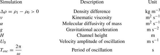
Dimensional quantities that define the flow are shown in table 1. Dimensional analysis results in four dimensionless numbers that govern the flow. The Reynolds number  $Re$, defined as
 \begin{equation} Re = \frac{{u}_b {H}} {{\nu}}, \end{equation}
represents the ratio of the inertial to viscous forces. Here,  $u_b$ is the buoyancy velocity,
 \begin{equation} {u}_b=\sqrt{{g} ' {H}}, \end{equation}
where  ${g} '$ indicates the reduced gravitational acceleration defined as
 \begin{equation} {g} ' = {g} \frac{\Delta{\rho}} {{{\rho }}_0}, \end{equation}
with  $\Delta {\rho } = \rho _1 - \rho _0 >0$ the density difference between the two fluids. The Schmidt number,
 \begin{equation} Sc = \frac{{\nu}} {{\alpha}}, \end{equation}
represents the ratio of kinematic viscosity of the fluid to molecular diffusivity of the density field. The Froude number  $Fr$, defined as
 \begin{equation} Fr = \frac{{U}_0 } {{u}_b }, \end{equation}
is the ratio between the free-stream velocity amplitude of oscillation  ${U}_0$ to the buoyancy velocity ${u}_b$. Lastly, we introduce the Keulegan–Carpenter number ( $KC_b$), which represents the ratio between the oscillation period ( $T_{osc}$) to the advection time scale associated with the propagation of the gravity current ( ${H}/{{u}_b}$). It is given as
 \begin{equation} KC_b = \frac{ {T}_{osc} {u}_b}{{H}}. \end{equation}
The Keulegan–Carpenter number  $KC_b$ can also be interpreted as a dimensionless period of the oscillations of the externally applied flow field.
Dimensional quantities that govern the fluid flow for our set-up.
We will use the governing equations (2.1)–(2.3) in dimensionless form by using
 \begin{equation} {u_i}^* = \frac{{u_i}}{{{u}_b} }, \quad {x_i}^* = \frac{{x_i}}{{H} }, \quad t^* = \frac{{t}}{{H/{u}_b} }, \quad p^* = \frac{{p}}{{\rho }_0 \, {{u}_b^2} }, \quad \rho ^* = \frac{ \tilde{\rho}} { \Delta {\rho} } \end{equation}
to make velocity, length, time, pressure and density dimensionless. Henceforth, we will use the dimensionless form of the equations and we eliminate the asterisk for convenience:
 \begin{gather} \frac{\partial {u}_j }{\partial {x}_j} = 0, \end{gather}
 \begin{gather} \frac{\partial {u}_i }{\partial t} + \frac{\partial ( {u}_i {u}_j)}{\partial x_j} =- \frac{\partial {p}}{\partial {x}_i} + \frac{1}{Re} \frac{\partial^2 {u}_i }{\partial {x}_j \partial {x}_j} - {\rho} \delta _{i2} + \frac{Fr}{KC_b} 2{\rm \pi} \cos \left( \frac{2{\rm \pi} t}{KC_b} \right) \delta _{i1}, \end{gather}
 \begin{gather} \frac{ \partial {\rho}}{\partial t} + \frac{ \partial ( {\rho} {u}_j)}{\partial {x}_j} = \frac{1}{Re Sc} \frac{ \partial ^2 {\rho}} {\partial {x}_j \partial {x}_j}. \end{gather}
 The forcing of the flow above the flat no-slip bottom wall by the oscillatory horizontal pressure gradient introduces a shear layer (the Stokes boundary layer) adjacent to the bottom boundary and an oscillating uniform free-stream velocity in the bulk above this layer. For later use (§ 4), it is instructive to compare the evolution of a gravity current in each of the limiting cases ( $KC_b\rightarrow 0$ and $KC_b\rightarrow \infty$) with the freely evolving gravity current. On the buoyancy time scale, the propagating gravity current experiences a uniform quasi-steady shear flow for $KC_b \rightarrow \infty$, while it does not, on average, experience a free-stream flow field for $KC_b \rightarrow 0$ since $T_{osc}\ll H/u_b$.
Let us first focus on the latter case,  $KC_b\rightarrow 0$. For high-frequency oscillations, the shear layer generated by the applied oscillating pressure gradient becomes very thin (see figure 2) and the duration of a single oscillation cycle is very short compared with the typical advection time scale associated with the buoyancy-driven dynamics of the gravity current. We expect that these high-frequency oscillations hardly affect the evolution of the gravity current on the buoyancy time scale, leaving its gross features almost untouched. The externally imposed oscillatory flow can nevertheless significantly affect the fluid motion near the stagnation point at the front of the current. The impact on details of the front dynamics and density redistribution will then always be significantly different compared with the freely evolving case, as will be illustrated in § 4.
However, when  $KC_b\rightarrow \infty$, the period of oscillations of the applied pressure gradient increases, and the Stokes boundary layer thickness grows and induces an ever thicker region with (quasi-steady) shear flow adjacent to the wall. The gravity current is then for a significant part embedded in and affected by this (quasi-steady) shear flow that, depending on the phase $\phi$ of the forcing cycle, has a free-stream velocity in the propagation direction of the gravity current ( $\phi =90^{\circ }$) or in the opposite direction ( $\phi =270^{\circ }$). Summarizing, the gross features of the dynamics of the freely evolving gravity current will show similarities with those of the externally forced cases with $KC_b$ small (high-frequency limit) and behaves completely differently compared with oscillatory-forced gravity currents with $KC_b$ very large (low-frequency limit). Visual evidence of these distinct behaviours for the low- and high-frequency ranges will be provided in § 4.
2.3. Parameter settings for our numerical studies
The dimensionless numbers governing freely evolving gravity currents are  $Re$ and $Sc$. The total number of grid points of a DNS of such 2-D gravity currents, for fixed $Sc$ and assuming proper resolution of the small-scale turbulence, scales with $O(Re)$ (while for 3-D gravity currents, we expect a scaling of the number of grid points with $O(Re^{9/4})$). Restrictions on the time step typically provides an additional cost proportional with $\sqrt {Re}$. Therefore, DNS studies are mostly limited to laboratory scale $Re$ numbers, even more so for 3-D turbulent gravity currents. Nonetheless, the results from such DNS studies are used to understand a variety of physical processes in more detail and contribute to the development of large-scale models suitable for higher $Re$ applications. For our DNS, we choose a fixed value of $Re=3000$. This selection allows for a feasible parameter study while aligning with the order of magnitude employed in earlier DNS studies of gravity currents (Härtel et al. Reference Härtel, Meiburg and Necker2000; Necker et al. Reference Necker, Härtel, Kleiser and Meiburg2002, Reference Necker, Härtel, Kleiser and Meiburg2005; Cantero et al. Reference Cantero, Balachandar, García and Ferry2006).
The Schmidt number displays significant variation, across several orders of magnitude for different environmental flows, since the diffusivity of the scalar that causes the density variation can differ significantly. For saline water,  $Sc \simeq 700$. In the case of thermal density differences in water, $Sc\simeq 7$, while in air, $Sc \simeq 0.7$ (which is also known as the Prandtl number). However, the lower range $Sc$ are mostly used for DNS studies of gravity currents to decrease the computational cost (typically $Sc= O(1)$). This is justified by Necker et al. (Reference Necker, Härtel, Kleiser and Meiburg2002) indicating that the integral properties of the current are independent of the actual $Sc$ value as long as it is not much smaller than one. Moreover, Birman, Martin & Meiburg (Reference Birman, Martin and Meiburg2005) stated that varying $Sc$ between 0.2 and 5 has an influence although it is small. For turbulent flows, the turbulent Schmidt number (the ratio of turbulent viscosity and turbulent diffusion coefficient) is typically around 0.7 to 1, while it increases for strongly stratified flows up to $Sc \simeq 5$. Ralston, Geyer & Lerczak (Reference Ralston, Geyer and Lerczak2008) found that the effective $Sc \simeq 2$ for a salt wedge in an estuary. Donzis et al. (Reference Donzis, Aditya, Sreenivasan and Yeung2014) showed, based on a high-resolution homogeneous isotropic turbulence simulation, that the turbulent Schmidt number is between 1 and 2 for Péclet number ( $Pe = Re \, Sc$) higher than 300, which is consistent with the findings by Necker et al. (Reference Necker, Härtel, Kleiser and Meiburg2002). In our study, we use $Sc=5$ in the majority of our simulations, but we also investigate the effect of $Sc$ by varying it in the range 1–20 with the aim of understanding the effect of diffusion on our results.
The external forcing is characterized by the Froude and Keulegan–Carpenter numbers, with the free-stream velocity amplitude characterized by  $Fr$ and the oscillation period by $KC_b$. The tidal Froude number, $Fr_T$, is the ratio between the maximum velocity in the tidal cycle and buoyancy velocity. It varies for different estuaries. In some estuaries, the tidal effect is smaller, and hence, $Fr_T$ becomes smaller. Typical values reported in the literature are $Fr_T \approx 0.35$ for the Mississippi River, $Fr_T \approx 0.4$ for the Connecticut River Estuary and $Fr_T \approx 0.45$ for the Tweed River (Ralston, Geyer & Lerczak Reference Ralston, Geyer and Lerczak2010). Meanwhile, $Fr_T$ is higher for some other estuaries. Examples are $Fr_T \approx 0.7$ for the Columbia River Estuary, the Fraser River and the Merrimack River Estuary, and $Fr_T \approx 0.8$ for the Snohomish River Estuary (Geyer et al. Reference Geyer, Lavery, Scully and Trowbridge2010). Therefore, we vary $Fr$ between 0.25 and 2 to understand the effect of the amplitude of the external oscillatory forcing on gravity currents.
Finally, we need to discuss an appropriate range of  $KC_b$ for our numerical simulations. Based on previous DNS studies (Härtel et al. Reference Härtel, Meiburg and Necker2000; Necker et al. Reference Necker, Härtel, Kleiser and Meiburg2002, Reference Necker, Härtel, Kleiser and Meiburg2005; Cantero et al. Reference Cantero, Balachandar, García and Ferry2006) on canonical freely evolving gravity currents, distinct characteristics are observed. Specifically, at the leading edge of the gravity current, a pronounced front emerges. This front is characterized by a steep increase in the current height, followed by a subsequent decrease towards the body of the gravity current. The location where the maximum current height occurs at the front is referred to as the head position. However, in nature, gravity currents are not always freely evolving and can be subjected to different external forces including an external oscillatory forcing. Salt wedges in estuaries are influenced by surface waves which typically have periods of the order of seconds as well as tidal forcing with a period of 12.42 or 24.84 hours on average. Recently, the effect of surface waves on gravity currents has been studied by using LES and $k-\epsilon$ models and experiments, and it was demonstrated that the presence of oscillatory forcing modifies the (turbulent) mixing happening at the front of the fresh-water current near the surface (Stancanelli et al. Reference Stancanelli, Musumeci and Foti2018a,Reference Stancanelli, Musumeci and Fotib; Cui et al. Reference Cui, Kamath, Wang, Han and Bihs2022; Marino et al. Reference Marino, Stagnitti, Stancanelli, Musumeci and Foti2023). However, the effect of surface waves on the heavier current near the bottom was less significant. The density distribution of the heavy front was actually similar in the absence of surface waves. Measurements of the salt intrusion in the Rotterdam Waterway (de Nijs, Pietrzak & Winterwerp Reference de Nijs, Pietrzak and Winterwerp2011) indicate significant differences in the front characteristics of the heavy current compared with freely evolving gravity currents. The front characteristics are also different compared with those of gravity currents affected by surface waves (Stancanelli et al. Reference Stancanelli, Musumeci and Foti2018a,Reference Stancanelli, Musumeci and Fotib; Marino et al. Reference Marino, Stagnitti, Stancanelli, Musumeci and Foti2023). For tidal forcing in the Rotterdam Waterway, with $H\approx 15\ {\rm {m}}$ and $u_b=1.5\unicode{x2013}1.8\ {\rm m}\ {\rm s}^{-1}$ (depending on the salt concentration), the main tidal constituent (M2) with a period of 12.42 h typically gives $KC_b \simeq 5000$. However, computationally, it is currently not feasible to use $KC_b$ numbers as high as 5000, since such simulations would require a domain with a very large aspect ratio and they would need very long integration times. We will show later that such simulations are fortunately not needed. Since distinct characteristics are observed between freely evolving gravity currents (Härtel et al. Reference Härtel, Meiburg and Necker2000; Cantero et al. Reference Cantero, Balachandar, García and Ferry2006) and the salt wedge in the Rotterdam Waterway (de Nijs et al. Reference de Nijs, Pietrzak and Winterwerp2011), where the oscillation period is large, it is necessary to explore the effect of different periods by varying $KC_b$. We will start with smaller periods of oscillation and increase the oscillation period to reach $KC_b$ values which can show similar flow features as those observed in estuarine salt intrusions. For this purpose, we will use $KC_b$ values of 5, 10, 25, 50 and 100.
3. Numerical approach
3.1. Numerical model
A variety of approaches are available for computational modelling of gravity currents, see, for example, the review by Meiburg, Radhakrishnan & Nasr-Azadani (Reference Meiburg, Radhakrishnan and Nasr-Azadani2015) and more recently the study by Van Reeuwijk, Holzner & Caulfield (Reference Van Reeuwijk, Holzner and Caulfield2019) using SPARKLE (Craske & Van Reeuwijk Reference Craske and Van Reeuwijk2015). We perform 2-D DNS to solve the governing equations (2.12)–(2.14) in non-dimensional form using the incompressible Navier–Stokes solver PARTIES (Biegert, Vowinckel & Meiburg Reference Biegert, Vowinckel and Meiburg2017a; Biegert et al. Reference Biegert, Vowinckel, Ouillon and Meiburg2017b). The code is based on a finite-difference approach, employing the fractional step method by Kim & Moin (Reference Kim and Moin1985), and uses a third-order explicit Runge–Kutta scheme with three substeps (Harten Reference Harten1997) to discretize the equation in time. The projection method (Chorin Reference Chorin1968) is used to ensure incompressibility, and the resulting Poisson equation is treated using a direct fast Fourier transform (FFT) solver at each Runge–Kutta substep (Biegert et al. Reference Biegert, Vowinckel and Meiburg2017a). The convective term in the momentum equation is explicitly solved, leading to the well-known Courant–Friedrichs–Lewy restriction. Spatial derivatives of the diffusion term in momentum equations are assessed using a second-order central finite differences scheme. A second-order upwind scheme is used to handle convective terms in both the momentum and transport equations. The diffusion term in both the momentum equation and the density transport equation is treated implicitly using second-order central differences in combination with a conjugate-gradient solver (Saad Reference Saad2003). Furthermore, the code has been parallelized using the MPI library to enhance performance. The code's accuracy and reliability have been rigorously validated through extensive testing, as demonstrated by Nasr-Azadani & Meiburg (Reference Nasr-Azadani and Meiburg2011).
3.2. Numerical set-up, boundary and initial conditions
Initially, the entire fluid is in a state of rest. At  $t=0$, a (virtual) gate is removed and due to buoyancy, a gravity current develops. Additionally, an external forcing in the form of an oscillatory pressure gradient is imposed in the along-channel direction. To apply periodic boundary conditions in the along-channel direction for pressure, velocity and density, we propose a computational set-up as sketched in figure 3. The middle section of the domain contains heavier fluid with a density $\rho = 1$ (the grey area in figure 3), while the left- and right-hand sides of the domain contain light fluid with a density $\rho = 0$. Our primary focus will be on the developing gravity current in the right half of the domain (in particular, the region with $x\ge 0$). The phase of the free-stream velocity, resulting from the imposed oscillatory pressure gradient, is initialized at $\phi =0^{\circ }$ (see figure 2). On the left-hand side of the domain ( $x<-170$), we effectively replicate (at $t=0$) the initial density distribution as on the right-hand side ( $x>-170$), but the gravity current (moving to the left) experiences an effective free-stream velocity with a $180^{\circ }$ phase difference compared with the right-hand side. This deliberate configuration provides us with a valuable opportunity to contrast the effect of oscillatory forcing starting from different phases. In the subsequent discussions, we will refer to the right part of the channel, except when the left part is explicitly mentioned. A no-slip boundary condition at the bottom wall and a stress-free boundary condition at the top boundary of the channel (a rigid free surface) are employed. The rigid free surface does not always accurately represent the free-surface behaviour for gravity currents in laboratory studies or estuaries, but it is commonly used for high-resolution numerical simulations of gravity currents.
Initial density field of the simulation set-up. The primary focus is the gravity current forming on the right-hand side of the domain ( $x>-170$). A visual representation of the interface between heavy and light fluid for the gravity current, which will form at a certain time after removal of the gate, is shown with a solid line. The gravity current at the left-hand side experiences oscillatory forcing with a phase difference of $180^{\circ }$ compared with the right-hand side.

The length of the domain is selected such that the gravity current does not extend to the sides of the domain during the full simulation covering 400 dimensionless time units. To include a minimum of four oscillation cycles of the externally imposed pressure gradient for the lowest frequency case ( $KC_b=100$), we need to choose the length of our channel equal to $L=680$ (and we use this for all the simulations). We use an equidistant Cartesian mesh with $\delta x = \delta y = l$. According to our convergence study, a non-dimensional grid size of $l=0.008$ for simulations with $Sc=1$ and $5$ is sufficient, while a grid size of $l=0.0025$ is necessary for simulations with $Sc=20$. Therefore, with our domain size of $680\times 1$ dimensionless units, we need approximately $10^7$ grid points for runs with $Sc=1$ and $5$, while we need approximately $10^8$ grid points for the simulations with $Sc=20$.
We performed our simulations on the Dutch Super Computer Snellius, using 128 cores. The simulations over 400 dimensionless time units using  $l=0.008$ required approximately 9000 CPU hours (approximately 71 wall-clock hours). For simulations with $l=0.0025$, the computational cost is nearly 528 000 CPU hours. We will cover a wide range of the parameter space by varying the three dimensionless numbers $KC_b$, $Fr$ and $Sc$. In the next sections, we present results from 13 simulations whose parameters are given in table 2, and we discuss (first qualitatively and later on quantitatively) the effect of varying these three parameters on the evolution and oscillatory dynamics of the gravity current. (For fresh and saline water, with $g'\approx 10^{-2}\ {\rm g}$, we obtain the following typical lab scale values: $H\approx 5$ cm and $u_b\approx 7\ {\rm cm}\ {\rm s}^{-1}$ based on $Re=3000$.)
The parameters for the simulations in this study.  $Re=3000$ is maintained for all simulations. In the next section, simulations 1 to 6 are compared to evaluate the effect of different forcing periods (by varying $KC_b$). To examine the impact of different ambient velocity amplitude ( $Fr$), results from simulations 1, 5, 7, 8 and 9 are compared for $Sc=5$. Additionally, the influence of diffusivity is analysed by contrasting results from simulation 1, 5, 10, 11, 12 and 13, where three different $Sc$ numbers are employed for two different $KC_b$ numbers. The simulations 1, 10 and 12 represent freely evolving gravity currents.

4. Qualitative description of gravity currents with oscillatory forcing
The dynamics of 2-D gravity currents, resulting from the canonical lock-exchange configuration, is well known. By introducing external oscillatory forcing, the parameter range describing the dynamical evolution of the gravity current will be extended with  $KC_b$ and $Fr$. Additionally, we need to consider the role of $Sc$ and the phase $\phi$ of the oscillating background flow. To illustrate qualitatively the propagation of the gravity current and the (fine-scale) density redistribution in the gravity current in this section, we focus mostly on the role of $KC_b$ and $\phi$, and keep $Sc$ and $Fr$ constant (their impact will be discussed in § 5).
The basic features of the dynamical evolution of such gravity currents will first be illustrated qualitatively by exploring and comparing snapshots of the density field. This provides visual insights in the propagation characteristics of such density currents and shows how external forcing and propagation of the density current affect the small-scale density redistribution. Additionally, snapshots of the local current height during the propagation of the gravity current are presented for different  $KC_b$. We compare the dynamical evolution of the density fields for simulations 1–6 (with $Re=3000$, $Fr=1$ and $Sc=5$, see table 2) at selected instances. (It should be noted that the horizontal and vertical scales of the snapshots in figures 4–9, in the Supplementary Material available at https://doi.org/10.1017/jfm.2024.1170, and in the movies are generally not equal. For example, in figure 4, the horizontal axis is approximately compressed by a factor of four, thus the aspect ratio of vertical to horizontal unit distance is $L_{AR}\approx 4.0$.)
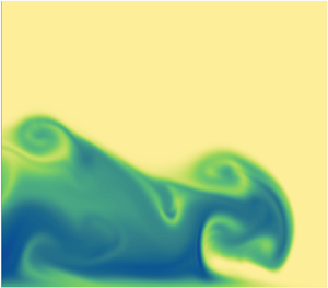
Dimensionless density fields for  $KC_b=50$ and $Fr=1$ at different phases of the imposed ambient flow ( $L_{AR}\approx 4.0$): (a) $\phi = 0^{\circ }$ at $t=50$; (b) $\phi = 90^{\circ }$ at $t=62.5$; (c) $\phi = 180^{\circ }$ at $t=75$; (d) $\phi = 270^{\circ }$ at $t=87.5$; (e) $\phi = 360^{\circ }$ at $t=100$ and (f) for the freely evolving gravity current, also at $t=100$. The value of the density (with $0 \le \rho \le 1$) is indicated by the colour bar.

Dimensionless density fields (with  $L_{AR}\approx 1.8$) (a) for the non-oscillating case and (b–f) those for different $KC_b$ (and $Fr=1$). For the oscillating cases, they are all obtained at the same phase of the forcing cycle, $\phi =90^{\circ }$. The time instance for the snapshots of the density fields are: (a) $t=96.25$; (b) $t=96.25$ (gone through 19.25 oscillation cycles; $KC_b=5$); (c) $t=92.5$ (9.25 cycles; $KC_b=10$); (d) $t=81.25$ (3.25 cycles; $KC_b=25$); (e) $t=62.5$ (1.25 cycle; $KC_b=50$) and (f) $t=25$ (0.25 cycle; $KC_b=100$). For panel (f), we plot the density field for $15 \le x \le 35$ since the front of the gravity current is located at $x\approx 24$ (thus including a substantial part of the tail of the current in the figure). The value of the density (with $0 \le \rho \le 1$) is indicated by the colour bar.

Dimensionless density fields for (a) the non-oscillating case and (b–f) those for different  $KC_b$ (and $Fr=1$), panels zoomed-in on the front of gravity current ( $L_{AR}=1$). For the oscillating cases, they are all obtained at the same phase of the forcing cycle, $\phi =90^{\circ }$. The time instance for the snapshots of the density fields are: (a) $t=96.25$; (b) $t=96.25$ ( $KC_b=5$); (c) $t=92.5$ ( $KC_b=10$); (d) $t=81.25$ ( $KC_b=25$); (e) $t=62.5$ ( $KC_b=50$) and (f) $t=25$ ( $KC_b=100$). The value of the density (with $0 \le \rho \le 1$) is indicated by the colour bar.

Dimensionless density fields (with  $L_{AR}\approx 1.3$) (a) for the non-oscillating case and (b–f) for different $KC_b$ ( $KC_b=5$ in panel b, $KC_b=10$ in panel c, $KC_b=25$ in panel d, $KC_b=50$ in panel e and $KC_b=100$ in panel f). For all cases, $Fr=1$. They are all shown for $t=100$, which coincides with $\phi =360^{\circ }$ for the oscillating cases. The front of the gravity current is well homogenized and has an inclined shape for $KC_b=50$ and $100$. The gravity current front is steep and stays slightly lifted for $KC_b=5$ and $10$. For $KC_b=25$, while the front is more inclined, the density current is not very homogenized at the front. The value of the density (with $0 \le \rho \le 1$) is indicated by the colour bar.

Illustration of the different methods to find the current height based on a snapshot of the density field for a simulation with  $KC_b=50$ and $Fr=1$, taken at $t=62.5$ and $\phi =90^{\circ }$ (with $L_{AR}\approx 1.7$). The black line indicates the local current height according to Shin et al. (Reference Shin, Dalziel and Linden2004), the grey line according to Anjum et al. (Reference Anjum, McElwaine and Caulfield2013) and the red line according to the proposed definition in this work using (4.3). The green line indicates the lifting height, defined in (5.1).

Local gravity current height  $h(x,t)$, (4.3), evaluated with a moving average procedure, for simulations with different $KC_b$ (and $Fr=1$) and for the freely evolving gravity current (with $L_{AR}\approx 3.0$). The results are displayed for: (a) $t=100$; (b) $t=200$; (c) $t=300$ and (d) $t=400$. The freely evolving gravity current shows the distinctive front shape (black lines). The gravity currents with $KC_b=5$ and $10$ (green and blue lines, respectively) illustrate a steep front shape. The front of the gravity current has a more inclined shape for simulations with $KC_b=50$ and $100$ (red and purple lines, respectively). $KC_b=25$ (orange line) represents an intermediate case.

4.1. Evolution of gravity currents during the forcing cycle
We start our exploration with an illustration of the gravity current evolution and the change in the (fine-scale) density structure during one complete forcing cycle. The redistribution of the density occurring at the front of the gravity current can be illustrated with snapshots of the density field at different phases of the forcing cycle (see also the animation of the density field evolution for  $50\le t\le 200$ in supplementary movie 1). Here, we consider the simulation with $KC_b=50$ (figure 4). In the beginning of the second oscillation cycle ( $\phi =0^{\circ }$, starting at $t=50$, see figure 4a), the gravity current propagates into the fresh-water region near the bottom of the channel. In the first half of the oscillation cycle ( $0^{\circ } \le \phi \le 180^{\circ }$), the gravity current propagates in the same direction as the imposed oscillatory flow. For $0^{\circ } \le \phi \le 90^{\circ }$, the imposed ambient flow tends to accelerate the gravity current and to decelerate it when $90^{\circ } \le \phi \le 180^{\circ }$. The imposed flow has a height dependent velocity in the (Stokes) boundary layer, which promotes differential advection. This is clearly visible for $\phi =90^{\circ }$ in figure 4(b). Heavy fluid has moved over lighter fluid near the bottom wall. We call this the lifting of the gravity current, and the area underneath the heavy current the lifting area. During the deceleration phase ( $90^{\circ } \le \phi \le 180^{\circ }$), the lifted part of the gravity current becomes unstable and starts to promote eddy formation, inducing enhanced (vertical) redistribution of the density field (see supplementary movie 1; $67\lesssim t\lesssim 77$ and $125\lesssim t\lesssim 135$). During the first half of the oscillation cycle, the thickness of the front of the gravity current is thinner (see figure 4a,b,e) compared with the freely evolving gravity current (shown in figure 4f).
In the second phase of the oscillation cycle ( $180^{\circ } \le \phi \le 360^{\circ }$), the externally applied flow acts against the propagation direction of the gravity current. This situation no longer supports lifting. Since an unstable flow configuration already emerged during the decelerating phase ( $90^{\circ } \le \phi \le 180^{\circ }$), the flow reversal provokes strong (vertical) density redistribution (figure 4c,d). As can be seen in supplementary movie 1, the heavy fluid sinks while the lighter fluid rises towards the upper interface of the gravity current. This lighter fluid subsequently moves further backwards towards the body of the gravity current due to relatively strong horizontal advection. This process takes place predominantly for $180^{\circ } \le \phi \le 270^{\circ }$ when the externally applied opposing flow accelerates to its maximum value at $\phi =270^{\circ }$ (figure 4d).
4.2. Coincidence of the imposed flow with the current propagation  $(0^{\circ }\le \phi \le 180^{\circ })$

From the previous description, we derive two distinct behaviours regarding the (small-scale) redistribution of the density field in the gravity current depending on the relative direction of the external forcing with respect to the propagation direction of the gravity current. When the oscillatory forcing (thus the externally imposed flow) coincides with the propagation direction of the gravity current, the gravity current is subjected to differential advection. This effect is most pronounced for  $\phi =90^{\circ }$, when the oscillatory forcing reaches a maximum value in the direction of the gravity current. The behaviour of the gravity current is completely different when it is subjected to opposing flow (with a maximum at $\phi =270^{\circ }$). This dissimilarity will be further explored in § 4.3, with density field snapshots at $\phi =360^{\circ }$ (or equivalently $\phi =0^{\circ }$) to illustrate the significant changes in the density distribution induced by the opposing flow. We shall first discuss the first half of the oscillation period.
Snapshots of the different density fields provide us with a qualitative picture of how differential advection affects the gravity current as a function of  $KC_b$ (see also the animation of the density field evolution for $0\le t\le 200$ in supplementary movie 2). Before we proceed, it is useful to discuss the approach to present our data in this section. We compare the density fields at the same phase of forcing, here at $\phi =90^{\circ }$, for simulations covering all $KC_b$. Therefore, we first select a time instance where, for all considered $KC_b$, an oscillation cycle concludes, thus $\phi =360^{\circ }$. Subsequently, we select instances that coincide at $\phi =90^{\circ }$ for the different $KC_b$, during the preceding oscillation cycle. By choosing $t=100$, we compare then the density fields at $\phi =90^{\circ }$ for $KC_b=5$, 10, 25, 50 and 100 at $t=96.25$, 92.5, 81.25, 62.5 and 25, respectively. For the canonical lock-exchange gravity current (without external forcing), we use the density field at $t=96.25$.
The density field of the gravity current forming from the classical lock-exchange set-up (see figure 5a) illustrates the same characteristics as those observed in earlier DNS studies (Härtel et al. Reference Härtel, Meiburg and Necker2000; Necker et al. Reference Necker, Härtel, Kleiser and Meiburg2002, Reference Necker, Härtel, Kleiser and Meiburg2005; Cantero et al. Reference Cantero, Balachandar, García and Ferry2006; Anjum, McElwaine & Caulfield Reference Anjum, McElwaine and Caulfield2013). At the leading edge of the gravity current, the height of the current increases steeply to a local maximum and subsequently to a local minimum in the body of the gravity current. The density fields at  $\phi =90^{\circ }$ for gravity currents in the presence of oscillatory forcing (figure 5b–f) show distinct shapes when compared with the freely evolving gravity current (figure 5a). Quite remarkably, the gravity currents for $KC_b\le 25$ have propagated a larger distance compared with the non-oscillatory case. Since we have a no-slip bottom, the magnitude of the externally imposed flow field must decrease towards the bottom and differential advection occurs. Heavier fluid farther from the bottom experiences a larger along-stream flow velocity than fluid near the bottom wall. Consequently, it moves over lighter fluid close to the bottom wall, particularly near the nose of the gravity current. This results in an apparent lifting of the gravity current, and the area beneath the gravity current is then called the lifting area. The lifting of the gravity current usually does not occur, or is almost negligible, for the freely evolving gravity current over a horizontal wall. The significant lifting is thus entirely due to the presence of oscillatory forcing and subsequent differential advection. We clearly observe the lifting and squishing of the gravity currents in figure 5(b–f). Lifting is weak for $KC_b=5$, but it increases with $KC_b$ because differential advection occurs for longer as the oscillation cycles become longer (thus larger $KC_b$). Additionally, the Stokes boundary-layer thickness becomes larger with increasing $KC_b$ (see figure 2). The layer of slowly moving light fluid becomes thicker, contributing to larger redistribution of light and heavy fluid beneath the heavy fluid at the front. For a quantitative discussion, see §§ 5.1 and 5.2.
In figure 6, we show the same density fields as in figure 5, but zoomed-in on the front of the gravity current. The horizontal and vertical length scales in the panels of figure 6 are identical (in contrast with figure 5) to appreciate the fine-scale structure within and beneath the gravity current, and the details of the front of the gravity current, including distinctly different (small-scale) redistribution of the density for the different cases.
In some of the snapshots shown in figure 6, in particular for  $KC_b=100$ and to a lesser extent for $KC_b=50$, there seems to be evidence of the presence of a Rayleigh–Taylor instability (see also figure 7b,c,d for $KC_b=5$, 10 and 25, respectively). For a closer inspection, the reader is also referred to the supplementary movies. This is an intriguing observation that deserves further exploration in future studies of both 2-D and 3-D DNS of oscillatory-forced gravity currents.
4.3. Gravity current propagation with opposing ambient flow ($180^{\circ }\le \phi \le 360^{\circ }$)

We now consider the situation where the propagating gravity current is subjected to an opposing externally imposed flow. This occurs for  $180^{\circ }\le \phi \le 360^{\circ }$. The maximum amplitude of the opposing flow occurs at $\phi =270^{\circ }$, but the influence of the opposing external flow is best appreciated when we consider its impact on advection and local redistribution of the density field at the end of the cycle with the opposing flow, i.e. at $\phi =360^{\circ }$. Hence, we compare the flow and density fields for each $KC_b$ always at the same instance after the release of the gravity current. The choice of the fixed times is dictated by the largest value of $KC_b$ and is typically $t=100$, 200, 300 or 400. We choose to illustrate advection and density redistribution with snapshots of the density field taken at $t=100$ for all cases (non-oscillating and $KC_b =$ 5, 10, 25, 50 and 100, respectively), see figure 7. These snapshots show a completely different structure compared with the case with a coinciding ambient flow.
Before proceeding with the qualitative comparison of the behaviour of oscillatory-forced gravity currents, it is necessary to address the representativeness of the density fields obtained during the relatively early stages after the release of the gravity current (for  $t\le 100$). The freely evolving gravity current propagates in a quasi-steady fashion, only driven by buoyancy due to the density difference between light and heavy fluid. Considering snapshots of the density field for this case taken at different instances, here at $t=100$ (see figure 7a), 200, 300 and 400 (see figures S10, S11 and S12 of the Supplementary Material), it can be observed that the front shape remains similar for all times, while the heavy current (front and body) is diluted due to entrainment of light fluid (and scalar diffusion). For the same times, the front of the gravity current in the presence of oscillatory forcing shows distinctively different patterns of small-scale density redistributions depending on the particular value of $KC_b$, but for each value of $KC_b$, this pattern of density redistribution does not strongly change with increasing time (except dilution by also diffusive processes). Signatures of flow instabilities (shear-induced eddy formation) and density-current lifting is clearly visible for $KC_b=5$, 10 and 25 (see figure 7b–d for $t=100$ and also the snapshots shown in figures S1–S9 of the Supplementary Material for $t=200$, 300 and 400, respectively). The main features of the evolution of the gravity current for $KC_b=50$ and 100 remain visible up to $t=400$. From this comparison, we can conclude that for the purpose of this qualitative comparison, we can rely on the density fields evaluated in the oscillation cycle ending at $t=100$.
We first consider  $KC_b\le 10$ (figure 7b,c). The externally induced oscillating flow acts against the propagation of the gravity current and could eliminate effects of density-current lifting by advection and enhanced (vertical) density redistributions. The duration of the opposing flow is apparently too short for these smaller values of $KC_b$ to achieve substantial (vertical) redistribution of density. The front of the gravity current thus always stays lifted and the interface (both beneath and above the current) is disturbed by eddies due to the presence of shear layers. Clearly, no full vertical density redistribution is achieved. Gravity currents in the presence of large-period oscillatory forcing (e.g. those with $KC_b=50$ and $100$, in figure 7e,f) experience strong changes in the density structure resulting in significant horizontal homogenization of the density field. Shear instabilities and eddies at the interface between heavy and light fluid have ample time to fully redistribute heavy and light fluid near this interface. These gravity currents are horizontally well homogenized at $t=100$, and their shapes are clearly different from the front shape of gravity currents with $KC_b\lesssim 25$ (figure 7b–d). Furthermore, the front of the gravity current has a clear inclined shape for $KC_b \ge 50$, which is similar to the inclined shape of salt intrusions at the ebb phase, as observed with salinity measurements in, for example, the Rotterdam Waterway reported by de Nijs et al. (Reference de Nijs, Pietrzak and Winterwerp2011). Therefore, we conclude that for $KC_b \gtrsim 50$, the behaviour of density redistributions at the front and the shape of the gravity current seem representative for salt intrusions as observed in environmental flows (usually in the presence of large-period forcing, typically with $KC_b \simeq 5000$). Lastly, for $KC_b=25$, see figure 7(d), the front is not very homogenized compared with for $KC_b=50$ and $100$, although the front clearly has a more inclined shape compared with the cases with $KC_b=5$ and 10.
4.4. The evolution of the local current height $h(x,t)$

The shape of the gravity current can be displayed and easily compared for different  $KC_b$ by finding the vertical position of the interface as a function of the horizontal coordinate. Consider first the situation of a density current without lifting. The vertical position of the interface can be estimated by defining a local current height for which different methods have been proposed in earlier studies by, for example, Shin, Dalziel & Linden (Reference Shin, Dalziel and Linden2004) and Anjum et al. (Reference Anjum, McElwaine and Caulfield2013). As suggested by Shin et al. (Reference Shin, Dalziel and Linden2004), the dimensionless local current height $h_{s}(x,t)$ is defined by the vertical integration of the density,
 \begin{equation} h_s (x,t) = \int_{0}^{1} \rho(x,y,t) \,{{\rm d} y}. \end{equation}
This method is not suitable in the presence of significant vertical density redistributions as observed by Anjum et al. (Reference Anjum, McElwaine and Caulfield2013). They proposed to define a spatially and temporally varying depth of the gravity current, denoted by  $h_a(x,t)$, using the available potential energy contained in the current. They derived $h_a(x,t)$ by first introducing the dimensionless centre of mass position $h_{cm}(x,t)$ of the heavy current in the vertical direction, which is defined as
 \begin{equation} h_{cm}(x,t) = \frac{\int_{0}^{1} \rho (x,y,t) y \, {{\rm d} y}}{\int_{0}^{1} \rho (x,y,t) \, {{\rm d} y}}. \end{equation}
This definition implicitly assumes that  $h_{cm}(x,t)$ is not defined right of the front position $X_{fr}$ as then $h_s(x,t) = 0$. We determined the front position by approaching the gravity current from the right-hand side and finding the position $x=X_{fr}$ of the first occurrence where $h_s(x,t)=0.005$ (varying this threshold value to determine $X_{fr}$ between 0.01 and 0.0025 affects the results by less than $1\,\%$). This implies that the value of $h_{cm}(x,t)$ is always clipped to zero for $x\ge X_{fr}$.
The local current height  $h_{a}(x,t)$ is then defined as twice the centre of mass height, $h_{a}(x,t)=2h_{cm}(x,t)$. However, gravity currents in the presence of an imposed oscillating flow field experience lifting, and therefore, $h_{a}(x,t)$ overestimates the local current height for the cases with lifting. To include this effect, we propose to quantify the current height $h(x,t)$ as the sum of the (vertical) centre of mass position $h_{cm}(x,t)$ of the heavy current and the local current height with respect to $h_{cm}(x,t)$ (which is not affected by the lifting height):
 \begin{equation} h (x,t) = h_{cm}(x,t) + 2 \frac{\int_{h_{cm}(x,t)}^{1} \rho (x,y,t) (y-h_{cm}(x,t)) \, {{\rm d} y}}{\int_{h_{cm}(x,t)}^{1} \rho (x,y,t) \, {{\rm d} y}}. \end{equation}
With our definition of  $X_{fr}$ and the constraint on $h_{cm}(x,t)$ introduced above, we immediately see that $h(x,t)=0$ for $x\ge X_{fr}$.
In figure 8, we provide a comparison of the local current height according to the methods introduced by Shin et al. (Reference Shin, Dalziel and Linden2004) and Anjum et al. (Reference Anjum, McElwaine and Caulfield2013), given by  $h_{s}(x,t)$ and $h_{a}(x,t)$, respectively, with the method introduced in this work for the local current height $h(x,t)$ at the front of a gravity current. It clearly shows the suitability of the modified measure introduced here (see the red line in figure 8).
The shape and evolution of gravity currents for a range of  $KC_b$ are explored by visualizing the local current height $h(x,t)$, representing the interface between heavy and light fluid, and computed according to (4.3), at $t=100$, 200, 300 and 400 (figure 9). Since we are not interested in the local details and features of the interface, such as instantaneous variations due to the presence of small vortices at the interface between the heavy and light fluid, we use a moving average of the data from 10 neighbouring grid cells to find the average current height. From figure 9, it is clearly seen that, for $KC_b = 50$ and 100, the interface maintains an inclined shape at the end of each cycle. This is not the case for smaller $KC_b$. In particular, for the cases with $KC_b=5$ and 10, there is a steep increase in the current height at the front of the gravity current. This is similar to the characteristics of the front shape seen for the freely evolving gravity current.
4.5. Summary
The density field  $\rho (x,y,t)$ and current height $h(x,t)$ for different simulations show that the gravity current is lifted in the first half of the oscillation cycle ( $0^{\circ }\le \phi \le 180^{\circ }$). During this part of the oscillation cycle, the externally imposed flow field aligns with the propagation direction of the gravity current. In the second half of the oscillation cycle ( $180^{\circ }\le \phi \le 360^{\circ }$), the unstable situation of heavy fluid being above light fluid causes enhanced (vertical) density redistributions within the gravity current. Enhanced density redistributions already start when the coinciding imposed flow starts to decelerate (for $\phi \ge 90^{\circ }$), and it is further strengthened when the imposed flow is opposite to the propagation direction of the gravity current.
From the comparison of both the density field of the gravity currents and the current heights for different  $KC_b$ (and for the freely evolving gravity current), three regimes, each with different behaviour of (small-scale) density redistributions, are observed. The front of the gravity current exhibits instabilities and additional redistribution of the density in the presence of the externally imposed oscillating flow field with $KC_b \lesssim 10$. The gravity current is lifted in the first half of the oscillation cycle and remains lifted throughout the whole cycle since the oscillation period is too short compared with the required time for full reattachment of the heavy current to the bottom of the channel. As a consequence, the subsequent phase with coinciding imposed external flow promotes lifting of the current again before reattachment occurs. Since the duration of the mean shear caused by the imposed flow is shorter, the shape of the current front is similar to the front shape for a freely evolving gravity current. Gravity currents with $KC_b \gtrsim 50$ show density redistributions similar in shape as those observed for salt wedges at the end of the ebb phase in estuarine flow configurations. Such salt wedges also occur, for example, in the Rotterdam Waterway with $KC_b \simeq 5000$. The front of the gravity current is well homogenized and has an inclined shape for $KC_b \gtrsim 50$. Lastly, the cases with $10 \lesssim KC_b \lesssim 50$ show an intermediate behaviour, where the current front has a more inclined shape compared with a smaller period of oscillations. However, the heavy current does not have enough time to become horizontally well homogenized.
5. The effect of varying $\boldsymbol {KC_b}$, $Fr$ and $Sc$ on gravity current dynamics


5.1. Impact of $KC_b$ on the lifting area and front shape

Observations from the evolving density field of several gravity currents, discussed in the previous section, uncovered a new phenomenon: the lifting of the gravity current. It happens primarily during the first half of the oscillation cycle ( $0^{\circ } \le \phi \le 180^{\circ }$). The second half of the oscillation cycle, for $180^{\circ } \le \phi \le 360^{\circ }$, is inherently unstable, since the heavy fluid has moved over light fluid in combination with the externally induced opposing flow, and lifting is no longer supported. In this section, we introduce a measure for and quantify the lifting area $A_{l}$ for gravity currents as a function of $KC_b$, thus as a function of the oscillation period of the external forcing. Additionally, we quantify the redistribution of density as well.
We define the dimensionless lifting height  $h_l(x,t)$ in a similar way as we determined the current height $h(x,t)$ in (4.3). More precisely, we quantify the lifting height as the difference of the (vertical) centre of mass position $h_{cm}(x,t)$ of the heavy current and the local current depth with respect to $h_{cm}(x,t)$:
 \begin{equation} h_l (x,t) = h_{cm}(x,t) - 2 \frac{\int_{0}^{h_{cm}(x,t)} \rho (x,y,t) (h_{cm}(x,t)-y) \, {{\rm d} y}}{\int_{0}^{h_{cm}(x,t)} \rho (x,y,t) \, {{\rm d} y}}. \end{equation}
 We use the lifting height  $h_l(x,t)$ to introduce a measure for the lifting area $A_l(t)$ beneath the gravity current as a function of time (note that $h_l(x,t)=0$ for $x>X_{fr}$), so that
 \begin{equation} A_l(t) = \int_{0}^{X_{fr}} h_l(x,t) \, {{\rm d}\kern0.06em x}. \end{equation}
The start of additional density transport due to the decelerating phase of the oscillatory forcing can typically be observed after reaching a maximum lifting area  $A_{l,max}$. We found that the lifting area becomes maximum at $\phi \approx 200^{\circ }$, $220^{\circ }$, $240^{\circ }$, $240^{\circ }$, $250^{\circ }$ for $KC_b = 100$, 50, 25, 10 and 5, respectively, and this occurs during each oscillation cycle. Therefore, we determine the maximum lifting area observed during each cycle for the full simulation and average $A_{l,max}$ over all cycles, and denote it with $\langle A_{l,max}\rangle$. With the simulation taking 400 time units, we average over $400/KC_b$ occurrences. A similar procedure is applied for the minimum lifting area $A_{l,min}$, since it is an indicator of whether the unstable configuration (heavy fluid over light fluid) continues to exist during the full cycle (which would imply $\langle A_{l,min}\rangle >0$) or the frontal region reaches a stable and vertically homogenized state within an oscillation cycle. The latter condition would mean that $\langle A_{l,min}\rangle \approx 0$.
The (averaged) maximum lifting area  $\langle A_{l,max}\rangle$, shown in figure 10(a), clearly increases with $KC_b$. For the freely evolving gravity current, the averaged maximum lifting area is very small, but not zero, due to a thin boundary layer above the no-slip wall. This very thin boundary layer contains light fluid left between the propagating gravity current and the no-slip wall, and is not related to the differential-advection mechanism discussed for the cases with $KC_b\gtrsim 5$. The data for the (averaged) minimum lifting area show that $\langle A_{l,min}\rangle >0$ for $KC_b=5, 10$ and $25$. Thus, a part of the lifting occurring during the first half of the forcing cycle survives during the second half of the forcing cycle. This is distinctively different for $KC_b=50$ and $100$, where the heavy current is already vertically homogenized before the next oscillation cycle starts.
(a) Average maximum lifting area  $\langle A_{l,max}\rangle$ (red symbols) and average minimum lifting area $\langle A_{l,min}\rangle$ (black symbols) as a function of $KC_b$ (and $Fr=1$). The freely evolving case is plotted on the vertical axis. (b) Scaling of the average maximum lifting area $\langle A_{l,max}\rangle$; the black dashed line indicates a scaling $\langle A_{l,max}\rangle \propto KC_b^{1.1\pm 0.1}$. The fit is based on nonlinear least squares from the data $KC_b\in$(5, 10, 25, 50, 100).

We take a closer quantitative look at the averaged maximum lifting area. Therefore, we replot the data for  $\langle A_{l,max}\rangle$ versus $KC_b$ logarithmically in figure 10(b), and the following approximate scaling is found: $\langle A_{l,max}\rangle \simeq 1.62\times 10^{-2} KC_b^{1.1}$. It is, thus, close to linear, for the range $5\le KC_b\le 100$. This scaling behaviour is consistent with the assumption that the lifting phenomenon is due to differential advection with, in this case, $Fr$ constant (thus, the same amplitude $U_0$ of the externally imposed oscillating flow in all cases). During one half of the oscillation cycle, with the externally imposed flow aligned with the propagation direction of the gravity current, the displacement of the heavy fluid in the front of the gravity current due to the externally imposed flow scales with $KC_b$. In contrast, the light fluid near the bottom wall only moves marginally due to the no-slip condition. An approximation for the lifting area would then take the form: $\langle A_{l,max} \rangle \propto \tfrac {1}{2}U_0 KC_b$ (or $\propto Fr KC_b$), consistent with our observation.
To quantify density redistributions in the presence of lifting and squishing phenomena, we focus on the gravity current front. It can be deduced from figure 9 that within a certain distance  $\Delta L$ (for example, $\Delta L = 15$) from the front of the gravity current, the current height is most dynamic and irregular. This allows us to illustrate and quantify the different density redistribution behaviours from this part of the gravity current. We define the extent of the gravity current front as the distance between the front position $X_{fr}$, defined in § 4.4, and $X_b=X_{fr} - \Delta L$. The precise choice of $\Delta L$ will be discussed later.
To illustrate the differences in density redistributions with varying  $KC_b$, we look at the spatially averaged current thickness. This quantity serves as a geometrical indicator of how much entrainment and redistribution of the density field happens between the heavy and light fluid in the gravity current. For this purpose, we take the current area within the front ( $X_b \le x \le X_{fr}$) and normalize it with $\Delta L = X_{fr}-X_b$ to find the average thickness of the current defined as
 \begin{equation} h_{t} (t) = \frac{1}{\Delta L}\int_{X_b}^{X_{fr}} [h(x,t) - h_l (x,t)] \,{{\rm d}\kern0.06em x}. \end{equation}
 A further indicator quantifying density redistributions is the average density in the gravity current front, denoted by  $\rho _a(t)$ and defined as
 \begin{equation} \rho_{a} (t) = \frac{1}{h_t(t)\Delta L}\int_{X_b}^{X_{fr}} \biggl(\int_{h_l(x,t)}^{h(x,t)}\rho (x,y,t) \,{{\rm d} y}\biggr) \,{{\rm d}\kern0.06em x}. \end{equation}
Both  $h_t(t)$ and $\rho _a(t)$ are evaluated with a predetermined length of the front region, $\Delta L = 15$. The choice of $\Delta L = 15$ might seem subjective at first glance, but we will explain this choice below.
In figure 11(a), we show  $h_t(t)$ for the freely evolving and the five different oscillatory-forced cases with $\Delta L = 15$. For all simulations, we show the results for $t=50, 100,\ldots, 400$. Similarly, we show $\rho _a(t)$ in figure 11(b) for the same times. The freely evolving case is shown by the black filled squares. The average thickness of the gravity current front decreases during the first part of the propagation phase (up to $t\approx 200$) before it tends to saturate at a constant value. The average density $\rho _a(t)$ in the gravity current front shows that, for increasing $KC_b$, the entrainment and redistribution of the density field in the gravity current front is enhanced compared with the freely evolving case, and we see that increasing $KC_b$ implies smaller values for $\rho _{a}(t)$. The curves shown in figure 11(b) suggest an approximately exponential decay of the average density, $\rho _a(t)\approx \exp (-t/\tau _{\rho })$, with $\tau _{\rho }$ a density relaxation time scale which depends on $KC_b$. We have computed $\ln \rho _a(t)$ for the range of $\Delta L$ between $5$ and $20$, and found that $\tau _{\rho }$ becomes independent of the choice of $\Delta L$ for $\Delta L\gtrsim 15$. This observation motivates our choice $\Delta L=15$ for this quantitative analysis. The inset in figure 11(b) shows $\tau _{\rho }$ for the range of $KC_b$ explored in this study. It is clear from the monotonic decrease of $\tau _{\rho }$ with $KC_b$ in the range $0\le KC_b\le 100$ that density homogenization occurs faster with increasing $KC_b$.
(a) Average current thickness  $h_t(t)$ of the gravity current front and (b) average density $\rho _a(t)$ in the gravity current front for the freely evolving gravity current and the five cases with an externally applied oscillating pressure gradient. For all cases, $Fr=1$. The horizontal extent of the gravity current front is taken as $\Delta L=15$. The inset in panel (a) shows the current thickness averaged over the times $200, 250, \ldots, 400$. Estimated error margins are included. The inset in panel (b) shows the density relaxation time $\tau _\rho$ for the same cases. For both insets, the values for the freely evolving case are on the vertical axis.

These conclusions can be further substantiated by considering the probability distribution of the density,  $P(\rho )$, in the same area (defined by $X_b\le x\le X_{fr}$ and $h_l(x,t)\le y\le h(x,t)$) used to compute $\rho _a(t)$. The density probability distribution is normalized using $\rho _a(t)$ such that $\int _0^1 P(\rho )\,{\rm d}\rho =1$ for each set of $KC_b$, $Fr$ and $Sc$ values. In figure 12, we show $P(\rho )$ at $t=100$ (figure 12a) and $t=200$ (figure 12b) for the freely evolving and oscillatory-forced gravity currents (with $Fr=1$ and $Sc=5$). The characteristics of the density redistributions for $KC_b=5$ and 10 are similar to those of the freely evolving gravity current, and enhanced density homogenization is observed for $KC_b=50$ and 100. Initially, the characteristics of the density redistributions for the case with $KC_b=25$ is close to the freely evolving case, but at later times, it shows similar homogenization of the density field as observed for the higher $KC_b$ runs. For $t\gtrsim 300$, the density probability distribution tends to a continuous uniform distribution given by $P(\rho )=1/(\rho _{max}-\rho _{min})$ for $\rho _{min}\le \rho \le \rho _{max}$ and zero elsewhere. Typically, $\rho _{min}\approx 0.1$ and $\rho _{max}\approx 0.5\unicode{x2013}0.7$ (the upper bound for small $KC_b$ and lower bound for large $KC_b$). In this interval, density values are more or less equally probable.
Density probability distribution  $P(\rho )$ as a function of $KC_b$ (and $Fr=1$, $Sc=5$) taken at (a) $t= 100$ and (b) $t=200$.

The data for  $h_t(t)$ support the observation from the previous section that we can distinguish three regimes. For $KC_b\lesssim 10$, the gravity current front remains always thicker than for the freely evolving case, while it is typically thinner for $KC_b\gtrsim 50$. The case $KC_b=25$ represents a transition regime with the thickness of the gravity current front being similar to that in the freely evolving gravity current. These observations suggest that, for $KC_b\lesssim 10$, entrainment and density redistributions mostly take place near the gravity current front, resulting predominantly in growth of its thickness. For larger $KC_b$, there is a strong interplay between entrainment and (vertical) density redistribution in the gravity current front, which promotes enhanced thickness, with strong horizontal advection. The latter mechanism removes parts of the top layer of the gravity current front to the rear, effectively resulting in a thinner but nevertheless lighter gravity current front.
We now consider average values of the current thickness,  $\langle h_t\rangle =\tfrac {1}{5}\sum _{n=4}^8 h(t=50n)$, thus using only the values outside the transient regime occurring for $t \le 150$. In the inset of figure 11(a), we show $\langle h_t\rangle$ (with an estimated error margin) obtained for $\Delta L=15$. The results support the conclusion above that, for $KC_b \le 10$, the average thickness of the front is larger compared with the freely evolving case and the other way around for $KC_b\ge 50$.
5.2. Effect of velocity amplitude (or $Fr$) of the externally imposed oscillating flow

The overall behaviour of gravity currents with  $KC_b \gtrsim 50$ show similarities with those of salt intrusions in estuaries. Therefore, we explored the effect of $Fr$ for simulations with $KC_b = 50$. It allows us to consider a substantial number of oscillation cycles (eight in total) to distinguish between transient effects (typically during the first three cycles) and quasi-steady oscillatory propagation of the gravity current during the last cycles. We consider $Fr = 0.25$, 0.50, 1 and 2 and the freely evolving case ( $Fr=0$). This comparison is thus based on the simulations 1, 5, 7, 8 and 9 in table 2. We will incorporate results from simulations where the initial phase of forcing is $\phi _{init} = 0^{\circ }$ and $180^{\circ }$. An animation of the density field evolution for $50\le t\le 200$ is shown in supplementary movie 3.
In §§ 4 and 5.1, we have discussed the basic mechanisms that affect the lifting height, its temporal evolution, the maximum lifting area  $A_{l,max}$ and the role of $KC_b$ (with $Fr$ kept fixed) on these quantities. In figure 13, we show $A_{l,max}$ at the end of each oscillation cycle for $Fr=0$, 0.25, 0.5, 1 and 2. From these data, it is clear that the first three cycles represent a transient period before the lifting area reaches an almost steady state. From the steady-state range, we get confirmation of our earlier hypothesized scaling of the maximum lifting area, $A_{l,max}\propto Fr KC_b$. This observation holds for both initialization phases, $\phi _{init}=0^{\circ }$ and $\phi _{init}=180^{\circ }$.
(a) Maximum lifting area  $A_{l,max}$ for each cycle of the oscillatory forcing of the different gravity currents under consideration ( $KC_b=50$). Two initializations are considered: $\phi _{init}=0^{\circ }$ (solid line) and $\phi _{init}=180^{\circ }$ (dotted line). Inset shows the vertical profile of the horizontal velocity of the externally imposed flow field at $\phi = 90^{\circ }$. The results from the steady-state range support our hypothesis $A_{l,max} \propto Fr$ and hardly depend on $\phi _{init}$.

To understand the effect of  $Fr$ on the distance travelled by the front of the gravity current, we investigate the front position $X_{fr}$, as defined in § 4.4, for different $Fr$ and compare it with the freely evolving case ( $Fr=0$). The front positions $X_{fr}$ as a function of time are shown in figure 14(a). To distinguish the effect of externally imposed oscillatory forcing on the front position, we determine the front position relative to the freely evolving case (with front position $X_{fr,0}$), denoted by $\Delta X_{fr}= X_{fr}-X_{fr,0}$ (figure 14b). The first three oscillation cycles are affected by transient behaviour and are, hence, disregarded in further discussions. To quantify the effect of the oscillatory forcing on $X_{fr}$, we consider the following cycle-averaged quantity:
 \begin{equation} \langle \Delta X_{fr}\rangle_n = \sqrt{\frac{1}{KC_b}\int_{nKC_b}^{(n+1)KC_b}\Delta X_{fr}^2\,{\rm d}t}, \end{equation}
with  $3 \le n \le 7$. It represents the averaged effect of the oscillatory forcing on $\Delta X_{fr}$ in each individual forcing cycle. The results for $\langle \Delta X_{fr}\rangle _{n}$ are shown in figure 14(c). We have computed the average $\langle \Delta X_{fr}\rangle =\tfrac {1}{2}(\langle \Delta X_{fr}\rangle _6+\langle \Delta X_{fr}\rangle _7)$ for the case with $\phi _{init}=0^{\circ }$. The results show that $\langle \Delta X_{fr}\rangle \propto Fr$ and advances the freely evolving case (see the solid curves in figure 14b,c). Furthermore, if we focus on simulations with varying $KC_b$ and keep $Fr=1$, we observe that $\langle \Delta X_{fr}\rangle \propto KC_b$. Carrying out the same approach for simulations with $\phi _{init} = 180^{\circ }$ shows again that $\langle \Delta X_{fr}\rangle \propto Fr$, but lags behind the freely evolving case (see the dotted curves in figure 14b,c). Our results provide strong indications that $\langle \Delta X_{fr}\rangle \propto Fr KC_b$, which makes sense intuitively, because $\langle \Delta X_{fr}\rangle$ will scale with the maximum velocity of the oscillation and the period of the oscillation. This suggests that differential advection is the key process determining the relative front position.
Front position of the gravity current for simulations with varying  $Fr$ with (a) $X_{fr}$, (b) front position for simulations with varying $Fr$ relative to the non-oscillating case, $\Delta X_{fr} = X_{fr}-X_{fr,0}$, and (c) period-averaged propagation speed $\langle \Delta X_{fr}\rangle _{n}$. The solid and dotted curves represent results with $\phi _{init}=0^{\circ }$ and $\phi _{init}=180^{\circ }$, respectively. The colour code indicates $Fr$.
$Fr$.

The frontal region of the gravity current becomes thinner and more diluted in the presence of oscillatory forcing with large  $KC_b$; see, for example, figures 7 and 11. To quantify the change in density within the current, we first introduce the total mass of the heavy fluid, $M_{Fr} (t) = h_t(t)\Delta L \rho _a(t)$, in the frontal region of the gravity current. Note that the dimensionless density of the light fluid is $\rho =0$ and of the heavy fluid $\rho =1$, and $0 \le \rho _a(t) \le 1$. The frontal region is defined by $X_b \le x \le X_{fr}$, with $X_b=X_{fr} - \Delta L$ (with $\Delta L = 15$), and $M_{Fr} (t)$ can be determined for each $Fr$. The relative mass difference in the frontal region compared with the freely evolving case is defined as $\Delta M_{Fr}(t)={[M_{Fr}(t)-M_0(t)]}/{M_{0}(t)}$, with $M_{0}(t)$ the total mass in the frontal region for the freely evolving gravity current. For $Fr\ge 0.5$, we find that the period-averaged value of $\Delta M_{Fr}(t)$ is negative, and for $Fr=0.25$, it is approximately zero. We start by considering $\phi _{init}= 0^{\circ }$. The period-averaged relative mass difference $\langle \Delta M_{Fr}\rangle _n$ in the frontal region is defined as
 \begin{equation} \langle \Delta M_{Fr}\rangle_n = \sqrt{\frac{1}{KC_b}\int_{nKC_b}^{(n+1)KC_b}\Delta M_{Fr}^2\,{\rm d}t}, \end{equation}
and is by definition positive. It increases significantly with increasing  $Fr$, see figure 15(a), and also shows transient behaviour for $t \le 150$. Therefore, we focus on the average of $\langle \Delta M_{Fr}\rangle _n$ for $200 \le t \le 400$, denoted by $\langle \Delta M_{Fr}\rangle = \tfrac {1}{4}\sum _{n=4}^7\langle \Delta M_{Fr}\rangle _n$. Due to the fact that the period-averaged value of $\Delta M_{Fr}(t)$ is typically negative, there is no ambiguity in the interpretation of $\langle \Delta M_{Fr}\rangle$ (which is always positive). Figure 15(a) shows an increase of $\langle \Delta M_{Fr}$ with $Fr$. For $\phi _{init}=180^{\circ }$, very similar behaviour is found for $\langle \Delta M_{Fr}\rangle _n$ (see figure 15a).
(a) Relative total mass difference  $\langle \Delta M_{Fr}\rangle _n$ for different $Fr$ (and $KC_b=50$) in the gravity current front averaged for each cycle compared with the freely evolving case. (b) Relative total mass through the gate $\langle \Delta M_{l,Fr}\rangle _n$ averaged for each oscillation cycle for the four values of $Fr$ relative to the freely evolving case. Solid lines, $\phi _{init}=0^{\circ }$; and dotted lines, $\phi _{init}=180^{\circ }$. The frontal region is defined by $X_b \le x \le X_{fr}$, with $X_b=X_{fr} - \Delta L$ (with $\Delta L = 15$).

Also here, we can consider the probability distribution of the density,  $P(\rho )$. In figure 16, we show $P(\rho )$ at $t=100$ (figure 16a) and $t=200$ (figure 16b) for the freely evolving and oscillatory-forced gravity currents with $KC_b=50$ and $Fr=0$, 0.25, 0.5, 1 and 2 (with $Sc=5$). We observe a gradual increase of the redistribution of the density with $Fr$ with a strong impact for $Fr\gtrsim 1$. This behaviour can also be observed qualitatively with animations of the density fields from simulations with varying $Fr$ (for $50\le t\le 200$) shown in supplementary movie 3.
Density probability distribution  $P(\rho )$ as a function of $Fr$ (and $KC_b=50$, $Sc=5$) taken at (a) $t=100$ and (b) $t=200$.

The decrease of the total mass in the frontal region supports our qualitative observations that the upper part of the gravity current front is pushed further backwards to its rear by the strong opposing flow (for  $KC_b=50$). The net advection of heavy fluid towards the frontal region is thus, on average, less in the presence of oscillatory forcing, which reduces the gravity current thickness and its average density. However, its propagation properties are dominated by differential advection, as discussed in the previous paragraph.
To further understand the bulk density transport, we compare the mass of heavy fluid passing through the gate (at  $x=0$) for gravity currents with $KC_b=50$ and $Fr=0.25$, 0.5, 1 and 2, and the freely evolving case ( $Fr=0$). To find the total mass of heavy fluid that passed the gate position, we introduce $M_{l,Fr}(t)$, defined as
 \begin{equation} M_{l,Fr} (t) = \int_{0}^{({1}/{4})L}\int_0^1 \rho (x,y,t) \,{{\rm d}\kern0.06em x} \,{{\rm d} y}. \end{equation}
In a similar way as before, we introduce  $\Delta M_{l,Fr}(t)= {[M_{l,Fr}(t)-M_{l,0}(t)]}/{M_{l,0}(t)}$, which also depends on $\phi _{init}$. For $\phi _{init}=0^{\circ }$, the period-averaged value of $\Delta M_{l,Fr}$ is positive, while it is negative for $\phi _{init}=180^{\circ }$ due to asymmetry of the forcing. The averaged total mass of heavy fluid passing through the gate is defined in a similar way as $\langle \Delta M_{Fr}\rangle$ and results shown in figure 15(b) suggest $\langle \Delta M_{l,Fr} \rangle \propto Fr$. For $\phi _{init}=0^{\circ }$, the total mass transport through the gate is always larger compared with the freely evolving case for $0.25\le Fr\le 2$. For $\phi _{init}=180^{\circ }$, the total mass transport through the gate is less for $0.25\le Fr\le 2$ compared with the freely evolving case (note that, according to our definition, $\langle \Delta M_{l,Fr} \rangle >0$). For both cases, the data show that $\langle \Delta M_{l,Fr}\rangle \propto Fr$, thus is connected with the excursion length of the oscillations and differential advection.
5.3. Effect of the Schmidt number on lifting area and propagation speed
The rate of molecular diffusivity changes according to the scalar that causes the density difference. Additionally, the effective Prandtl–Schmidt number also changes for different applications and conditions in estuaries with different stratification. Therefore, we are interested to see the effect of diffusivity on mass transport (of heavy fluid) and gravity current dynamics. For this purpose, we carried out simulations with  $Sc=1$, 5 and 20, while we kept the other parameters fixed: $KC_b=50$, $Fr=1$ and $Re=3000$.
To show the effects of varying  $Sc$ on the front position of the gravity current, we only focus on oscillatory-forced gravity currents with $\phi _{init}=0^{\circ }$. The cycle-averaged front position of the gravity current,
 \begin{equation} \langle \Delta X_{fr}\rangle_n = \sqrt{\frac{1}{KC_b}\int_{nKC_b}^{(n+1)KC_b} {[X_{fr,1} - X_{fr,0}]^2\,{\rm d}t}}, \end{equation}
represents an averaged propagation difference between the gravity current in the presence of oscillatory forcing (with front position  $X_{fr,1}$) compared with the freely evolving gravity current (with front position $X_{fr,0}$) for varying $Sc$. The average $\langle \Delta X_{fr}\rangle$ over the last two forcing cycles ( $300 \le t \le 400$) shows that the cycle-averaged front position of the gravity current advances the freely evolving case by a similar amount for the three values of $Sc$, see figure 17(a), and hardly influences the relative propagation of gravity currents. The maximum lifting area $A_{l,max}$ of the gravity currents, using the definition from (5.2), shows a similar trend for different $Sc$ (see figure 17b). They show a transient behaviour, where $A_{l,max}$ increases for $n \le 3$, before saturating. Since the molecular diffusion for $Sc=1$ is higher, the gravity current becomes more diluted at the front while differential advection occurs. Therefore, we expect that $\langle A_{l,max} \rangle$ will be somewhat smaller for $Sc=1$ compared with $Sc=5$ and 20.
(a) Period-averaged front position of the oscillatory-forced gravity current with respect to propagation of the freely evolving gravity current,  $\langle \Delta X_{fr}\rangle _{n}$, (b) maximum lifting area of gravity current, $A_{l,max}$, for simulations with different $Sc$ and (c) relative total mass difference $\langle \Delta M_{Sc} \rangle _n$ for different $Sc$ at the gravity current front for each cycle compared with the freely evolving case. The initial phase of the forcing is $\phi _{init} = 0^{\circ }$ and the frontal region is defined by $X_b = X_{fr} - \Delta L \le x \le X_{fr}$ (with $\Delta L = 15$). The colour indicates $Sc$.
$Sc$.

The relative mass of heavy fluid in the frontal region is defined as  $\Delta M_{Sc}(t)={[M_{Sc}(t)-M_{Sc,0}(t)]}/{M_{Sc,0}(t)}$, with $M_{Sc,0}(t)$ the total mass in the frontal region of the freely evolving gravity current for the Schmidt number under consideration. The cycle-averaged relative mass of heavy fluid in the frontal region for varying $Sc$ is expressed as
 \begin{equation} \langle \Delta M_{Sc}\rangle_n = \sqrt{\frac{1}{KC_b}\int_{nKC_b}^{(n+1)KC_b}\Delta M_{Sc}^2\,{\rm d}t}. \end{equation}
Also for the cases evaluated here, there is a reduction in the amount of mass in the frontal region, so there is no ambiguity in the meaning of  $\langle \Delta M_{Sc}\rangle _n$. The cycle-averaged relative mass $\langle \Delta M_{Sc}\rangle _n$ shows a significant decrease for $Sc=1$, see figure 17(c), while those for $Sc=5$ and 20 saturate. This is also reflected in the probability distribution of the density $P(\rho )$ for different $Sc$, not shown. The averaged value of $\langle \Delta M_{Sc}\rangle _n$ for $300 \le t \le 400$ shows that the relative mass at the front region for each $Sc$ is significantly reduced, particularly for $Sc=5$ and 20. This indicates that the relative mass difference at the frontal region between the oscillating and freely evolving case is larger for higher $Sc$ values since the freely evolving gravity current is less diluted at the front for those cases.
6. Discussion
We have investigated the effect of externally imposed oscillatory forcing on gravity currents using 2-D DNS. Our study focused on the effect of  $KC_b$, $Fr$ (both characterizing the oscillatory forcing) and $Sc$ on the dynamics of the gravity current and its (fine-scale) density redistribution properties. The Reynolds number of the flow, based on the buoyancy velocity $u_b$, was kept constant, $Re=3000$.
6.1. Summary of the main results
A qualitative exploration of the overall characteristics of periodically forced gravity currents, with  $Fr=1$, $Sc=5$ and varying $KC_b$, showed the existence of three distinct regimes. For $KC_b \lesssim 10$, the flow shows instabilities and density redistributions at the front of the gravity current similar to the freely evolving gravity current. However, for $KC_b \gtrsim 50$, the flow shows different advective density transport and (vertical) density distributions that are reminiscent of those observed for some propagating salt intrusions at the end of the ebb phase in estuaries. Specifically, the front of the gravity current is well homogenized and inclined. For $10 \lesssim KC_b \lesssim 50$, the flow displays intermediate characteristics with an inclined front but with less efficient density redistribution properties than for larger $KC_b$ values.
A detailed quantitative analysis focused on the role of  $KC_b$ and $Fr$ on key characteristics: the front position, the averaged maximum lifting area, the current thickness, the density in the front and mass deficits in the front of the gravity current. In general, the front displacement after a full oscillation cycle is hardly affected by the oscillatory background flow, but the transport of mass is reduced because both the thickness and the density at the front are lower when oscillations are present. This quantitative analysis supports our qualitative observation of three distinct regimes, and further points to differential advection as the crucial mechanism to produce the distinct characteristics. First, the gravity current is lifted by differential advection when the background flow coincides with the propagation direction of the gravity current, resulting in an unstably stratified water column. When the background flow reverses, the unstable stratification translates into vigorous density redistributions in the gravity current. Although the lifting area varies linearly with $KC_b$, the effects of the density redistributions quantified through, for example, the current thickness and the relaxation time of the density at the front vary in a nonlinear way. In fact, we see a difference in the dependence of these quantities with $KC_b$ for $KC_b \lesssim 10$ and for $KC_b\gtrsim 50$. For $KC_b \lesssim 10$, the average current thickness is larger than for the freely evolving case; for $KC_b\gtrsim 50$, it is smaller. For all oscillatory-forced cases, we observe an increased reduction of the density at the front compared with the freely evolving case with increasing $KC_b$.
The regime for  $KC_b \gtrsim 50$ was further explored through simulations with $KC_b = 50$ and varying $Fr$ (i.e. the amplitude of the oscillation). The mass of heavy fluid in the gravity current front is smaller than in the freely evolving gravity current, and becomes even smaller for increasing $Fr$. This deficit tends to be proportional to $Fr$ for the range considered in this study. In a similar spirit, we have explored the total mass of heavy fluid that passes the gate position compared with the freely evolving gravity current. For $\phi =0^{\circ }$, more heavy fluid passes through the gate compared with the freely evolving case, and for $\phi =180^{\circ }$, less fluid passes the gate. In both cases, the mass deficit scales with $Fr$, suggesting that differential advection plays a crucial role in mass transport for large $KC_b$. The impact of the Schmidt number, which took the values $Sc=1$, 5 and 20, turns out to be limited. The average lifting area and mass of heavy fluid in the frontal region is similar for $Sc=5$ and 20. These quantities are only affected when diffusion of mass is significant, as is the case for $Sc=1$.
6.2. A different cross-section of the $Fr-KC_b$ parameter space

For salt intrusions in estuaries,  $Fr$ (quantifying $U_0$) and $KC_b$ (quantifying $T_{osc}$) are fully independent quantities. The local geometrical and bathymetrical conditions of the estuary determines $Fr$, and the tidal frequency determines $KC_b$. In the present study, we either kept $KC_b$ fixed and varied $Fr$ (mimicking the estuarine configuration) or the other way around to explore the transition from the freely evolving to the oscillatory-forced gravity current and the different transition regimes, if any. Both approaches imply that the dimensionless amplitude of the forcing term, which is proportional to $Fr/KC_b$, varies for each combination of $Fr$ and $KC_b$. A set of simulations has been performed keeping $Fr/KC_b=0.02$ and varying $KC_b$ in the range from 5 to 100 to isolate the effect of the oscillating time period on the flow dynamics. The main observations are (see figures S13–S16 in the Supplementary Material): up to $KC_b=25$, the gross behaviour of the gravity current is very similar to the freely evolving gravity current, and the gravity current front has a similar shape and lifting is virtually absent (except for $KC_b=25$). Also, the average current thickness $h_t(t)$ and average density in the gravity current front, $\rho _a(t)$, show very similar behaviour. Differences emerge for $KC_b\gtrsim 50$. The average maximum lifting area $\langle A_{l,max}\rangle$ is significant, and we still observe $\langle A_{l,max}\rangle \propto Fr KC_b$.
6.3. Qualitative comparison between 2-D and 3-D simulations for $Fr=1$ and $KC_b=5$


We have made a qualitative comparison between results from one of our 2-D simulations (with  $Fr=1$, $KC_b=5$) with two 3-D simulations under the same forcing conditions. For the 3-D simulations, we applied either periodic or no-slip lateral boundary conditions. The width of the channel was equal to the height of the channel. The simulations have been carried out over 50 time units. The comparison is based on snapshots of the density field at the midplane of the channel in our 3-D simulations. The front speed of the gravity current is marginally higher (few percent) for the 3-D oscillatory-forced gravity current compared with its 2-D analogue. The shape and steepness of the front of the gravity current is very similar for the three cases. The lifting and squishing processes are clearly visible in the 3-D simulations and comparable with our observations from the 2-D simulation, and the average thickness of the front of the gravity current is similar for the 2-D and 3-D periodic case, while it is slightly thinner for the 3-D case with no-slip lateral boundaries. The vigorous mixing processes occur in all three cases during opposing flow conditions (including phenomena that suggest the presence of Rayleigh–Taylor instabilities), but the density redistribution in the front region of the 2-D gravity current is more strongly governed by small-scale coherent vorticity patches. In the 3-D gravity currents, these patches are quickly destroyed, most likely due to intrinsic 3-D dynamics of vortex tubes and lateral instabilities. In summary, we can conclude that our 2-D simulation provides good insight to the main characteristics of the dynamics of an oscillatory-forced gravity current under current conditions ( $Fr=1$ and $KC_b=5$). A further exploration of the $Fr-KC_b$ parameter regime might be worthwhile to confirm these observations.
There is one major difference between the three different simulations discussed above and this is related to the presence of vortical structures. For 2-D simulations, the Kelvin–Helmholtz billows are and remain clearly present for many combinations of  $Fr$ and $KC_b$. For our case with $Fr=1$ and $KC_b=5$, we observe that, for the 3-D case with periodic lateral boundary conditions, similar Kelvin–Helmholtz billows are present up to $t\approx 15$, but they gradually disappear for $t\gtrsim 15$. For the 3-D case with no-slip lateral sidewalls, shear-induced vortical structures generated near the front of the gravity current are quickly destroyed, most probably due to the presence of the lateral no-slip walls (at a distance $H$/2 from the midplane), which does not easily support the presence of shear-induced vortex tubes perpendicular to it. As is the case for the freely evolving gravity current, the presence or absence of the shear-induced vortices at the gravity current interface does not have a significant effect on the gross features of the gravity current dynamics, mixing properties and front shape. It also has no visible impact on the lifting and squishing phenomena.
Although qualitatively 2-D and 3-D oscillatory-forced gravity currents behave similarly (except for the presence of relatively persistent 2-D vorticity patches in the 2-D case), we expect that a more extensive (and computationally expensive) exploration of the  $Fr-KC_b$ parameter regime is needed to understand details of the turbulent mixing processes in combination with lifting and squishing. This should be a topic for future studies and would allow a better connection with laboratory experiments and field observations.
6.4. Prospects for laboratory experiments
We have addressed the dynamics of gravity currents under oscillatory forcing with numerical studies. One could wonder whether the observed phenomena, while consistent with similar processes, reflect reality sufficiently well. Answers can undoubtedly be obtained from physical experiments allowing a study of a full 3-D system and also for larger values of the Reynolds number (based on the buoyancy velocity of the flow). This is challenging but not entirely impossible provided suitable (infrastructural) facilities are available. For this purpose, we need a large tank for the lock-exchange experiments, allowing the gravity current to evolve over sufficiently long time scales and periods of oscillatory forcing (particularly relevant for large  $KC_b$). Comparing with current day laboratory experiments on gravity currents (see, for example, Sher & Woods Reference Sher and Woods2015; Ottolenghi et al. Reference Ottolenghi, Adduce, Roman and Armenio2017; Longo et al. Reference Longo, Ungarish, Di Federico, Chiapponi and Petrolo2018; Maggi, Adduce & Negretti Reference Maggi, Adduce and Negretti2022; Chiapponi et al. Reference Chiapponi, Zemach, Petrolo, Ungarish and Longo2023), we need for our application a tank with a length between approximately 50 and 100 m (provided the height of the tank is in the range between 0.1 m and 0.2 m, according to the experimental works mentioned above). For practical reasons, this is not immediately possible. The sheer length will also put severe constraints on the application of optical measurement tools to quantify the flow dynamics and (turbulent) mixing properties as a large section of the tank needs to be visualized at once (typically 5–10 m in length). Additionally, dynamic translation of the optical system is required to track the developing gravity current over many oscillation cycles. The current 2-D numerical study can already provide valuable insight and input for the design of this kind of experimental campaign.
7. Conclusion
Although this study is limited to 2-D DNS and relatively low Reynolds numbers, our results allow us to discern fundamental effects of an externally imposed oscillatory forcing and compare with previous results from literature. One of the interesting observations is that, for the parameter settings  $Re=3000$, $Sc=5$, $KC_b=50$ and $0.25\le Fr \le 2$, we enter a regime that might be representative for salt intrusions in environmental flows. Exploration of this regime in more depth requires an extension to fully 3-D simulations, including full 3-D (fine-scale) density redistribution processes (i.e. 3-D mixing), flows with substantially higher Reynolds numbers to arrive to the turbulent regime, and gravity currents under oscillatory forcing in stratified ambients. Such numerical studies can provide further insights into the interaction of the gravity current with the 3-D Stokes boundary layer, the role of vorticity in the development of these boundary layers, and its impact on lifting and mixing. Additionally, the variation of the lifting process in spanwise direction (whether it is similar, as observed for the lobe-and-cleft structure including the spanwise wavelength, or not), and the presence, characteristics and impact of the Rayleigh–Taylor instability and associated mixing processes can then be explored in more detail. For a better understanding of more realistic turbulent geophysical gravity currents, interesting future research directions could include effects of background rotation and non-flat bottom walls. Additionally, and to get closer to environmental configurations, a mean flow should be added to the current externally imposed oscillatory forcing to generate a so-called arrested gravity current. These are the topics of current studies.
Supplementary material and movies
Supplementary material and movies are available at https://doi.org/10.1017/jfm.2024.1170.
Acknowledgement
E.M. gratefully acknowledges support by the NSF grant CBET-2138583. The authors thank R. Uittenbogaard for helpful discussions and suggestions.
Funding
This work is part of the Perspectief Program SALTIsolutions, which is financed by NWO Domain Applied and Engineering Sciences (2022/TTW/01344701) in collaboration with private and public partners. This work used the Dutch national e-infrastructure, supported by the SURF Cooperative through grant number EINF-4757.
Declaration of interests
The authors report no conflict of interest.


 Open access

