


Impact Statement
Climate projections increasingly rely on combining many climate models, yet these models are not equally reliable or independent. This study shows how machine learning can improve multi-model ensemble predictions while keeping model contributions visible. Using CMIP6 temperature and precipitation simulations evaluated against ERA5, we compare arithmetic averaging with Ridge regression, random forest, and an adaptive gating approach. The gating model improves predictive skill, especially for temperature, while revealing where trust is concentrated in particular models, clusters, regions, or seasons. These diagnostics help researchers understand when data-driven weighting is useful rather than treating machine learning as a black box. The framework offers a transparent pathway for building more accountable climate ensemble tools for research and decision support in future climate assessments.
1. Introduction
Multi-model ensembles are a central tool in climate science, particularly for synthesizing uncertainty and producing robust climate projections. In large coordinated experiments such as CMIP, the dominant practice is to combine models using simple arithmetic averaging, implicitly treating each model as an independent and equally plausible representation of the climate system. This “model democracy” approach remains widely used due to its simplicity, transparency, and long-standing institutional acceptance.
However, extensive work in climate science has shown that these assumptions rarely hold in practice. Climate models are neither independent nor equally skillful: many share code bases and parameterizations, and their performance varies substantially across variables, regions, and temporal scales (Sanderson et al., Reference Sanderson, Knutti and Caldwell2015; Knutti et al., Reference Knutti, Sedláček, Sanderson, Lorenz, Fischer and Eyring2017). As a result, equal weighting can lead to over-representation of closely related model families and suboptimal ensemble predictions. This has motivated a large body of research on performance-based and dependence-aware weighting schemes for climate ensembles (Knutti et al., Reference Knutti, Sedláček, Sanderson, Lorenz, Fischer and Eyring2017; Slater et al., Reference Slater, Villarini and Bradley2017).
In parallel, recent studies have increasingly applied machine learning methods for climate ensemble post-processing, including linear regression, random forests (RFs), and neural networks (Dey et al., Reference Dey, Sahoo, Kumar and Remesan2022; Pakdaman et al., Reference Pakdaman, Babaeian and Bouwer2022; Kumar and Dwarakish, Reference Kumar and Dwarakish2025). These approaches often report improved predictive accuracy compared to unweighted means, especially for near-surface temperature and hydrological variables. However, most ML-based ensemble studies focus primarily on aggregate skill metrics and provide limited insight into how individual climate models contribute to the final prediction. This lack of interpretability makes it difficult to assess robustness, diagnose failure modes, or connect data-driven improvements back to physical understanding.
In this paper, we present an application-oriented framework for interpretable ensemble learning using CMIP6 simulations and ERA5 reanalysis. We track how machine learning methods reallocate trust across individual climate models and across coarse groupings of models defined by their climatological behavior. Our goal is to understand when machine learning is epistemically useful for climate ensemble post-processing, and which models drive those improvements.
We structure our analysis around three applied research questions:
-
• RQ1 (Structure): To what extent do simple climatological summaries reveal coarse groupings among CMIP6 models, and how useful are these groupings for interpreting ensemble learning behavior?
-
• RQ2 (Skill): How do machine learning ensemble methods compare to arithmetic averaging for predicting near-surface temperature and precipitation?
-
• RQ3 (Interpretability): Which climate models receive the highest effective weights under machine learning, and how do these weights vary across clusters, spatial regions, and seasons?
2. Data and experimental design
2.1. Climate model and observational data
We use monthly near-surface air temperature (tas) and precipitation (pr) from 25 CMIP6 global climate models, covering the historical period 1948–2014. The selected models span a wide range of modeling centers and include both Earth system models and coupled general circulation models. All model outputs are regridded to a common
$ 1{}^{\circ}\times 1{}^{\circ} $
 latitude–longitude grid to ensure spatial consistency across models.
As observational reference, we use the ERA5 reanalysis product, which provides globally complete and physically consistent estimates of atmospheric variables based on data assimilation of satellite and in situ observations. ERA5 is treated as the target for supervised learning and model evaluation. For both CMIP6 and ERA5, we compute global area-weighted means using cosine latitude weights.
2.2. Climatological feature construction
To characterize systematic differences among climate models, we compute each model’s long-term climatological mean for temperature and precipitation. Specifically, for each CMIP6 model
$ m $
 , we define

where
$ {x}_{m,t,i,j} $
 denotes the variable value at time
$ t $
denotes the variable value at time
$ t $
 and grid cell
$ \left(i,j\right) $
and grid cell
$ \left(i,j\right) $
 , and
$ {w}_{ij}=\cos \left({\phi}_{ij}\right) $
, and
$ {w}_{ij}=\cos \left({\phi}_{ij}\right) $
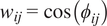 are latitude-based area weights. These climatological summaries provide a low-dimensional representation of each model’s large-scale behavior and are used as features for clustering.
We intentionally adopt a low-dimensional representation based on long-term global climatological means. Our goal is to construct a coarse, interpretable partition that can be directly related to how ensemble learning redistributes weights. A scalar global mean is the simplest such feature and the most transparent for tracing learned weights. This choice reflects a trade-off between representational richness and interpretability: while higher-dimensional features (e.g., regional or decadal statistics) may capture more detailed structure, they also make it more difficult to attribute learned weights back to physically meaningful differences among models. We acknowledge this limitation explicitly; exploring richer feature spaces is an important direction for future work.
2.3. Train–validation–test splitting
All supervised learning experiments follow a time-ordered split to avoid temporal leakage. The full time series is divided into a training period (1948–1998), a validation period (1999–2005), and a test period (2006–2014). Machine learning models are trained on the training set, hyperparameters are selected using the validation set, and all reported performance metrics are computed on the held-out test period.
2.4. Ensemble learning methods
We compare four ensemble post-processing strategies. As a baseline, the arithmetic multi-model ensemble (AMME) prediction is computed as the simple average across all CMIP6 models:
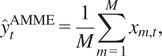
where
$ M $
 denotes the number of models and
$ {x}_{m,t} $
denotes the number of models and
$ {x}_{m,t} $
 the prediction from model
$ m $
the prediction from model
$ m $
 at time
$ t $
at time
$ t $
 .
.
We then fit a Ridge regression model to learn a global linear weighting of models,
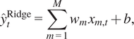
where weights
$ {w}_m $
 are estimated by minimizing squared error subject to an
$ {\mathrm{\ell}}_2 $
are estimated by minimizing squared error subject to an
$ {\mathrm{\ell}}_2 $
 regularization penalty. Hyperparameter
$ \alpha $
regularization penalty. Hyperparameter
$ \alpha $
 is selected from
$ \left\{\mathrm{0.01,0.1,1.0,10.0,100.0}\right\} $
is selected from
$ \left\{\mathrm{0.01,0.1,1.0,10.0,100.0}\right\} $
 on the validation set. This formulation yields an interpretable mapping between individual climate models and their contributions to the ensemble prediction. The
$ {\mathrm{\ell}}_2 $
on the validation set. This formulation yields an interpretable mapping between individual climate models and their contributions to the ensemble prediction. The
$ {\mathrm{\ell}}_2 $
 penalty distributes weight broadly across models, preventing any single model from dominating; a sparser alternative such as LASSO (
$ {\mathrm{\ell}}_1 $
penalty distributes weight broadly across models, preventing any single model from dominating; a sparser alternative such as LASSO (
$ {\mathrm{\ell}}_1 $
 ) would perform automatic model selection and is a natural direction for future work.
To capture nonlinear interactions among models, we also apply an RF regressor using model outputs as input features. We use
$ {n}_{\mathrm{estimators}}=600 $
 trees with
$ \min \_\mathrm{samples}\_\mathrm{leaf}=2 $
trees with
$ \min \_\mathrm{samples}\_\mathrm{leaf}=2 $
 . Variable importance scores are computed as the mean decrease in impurity (MDI) averaged over all trees and normalized to sum to 1; they quantify the relative contribution of each CMIP6 model to the RF prediction.
Finally, we implement a continuous gating mixture model that learns a convex combination of Ridge and RF predictions. The gated prediction is

where subscripts
$ \left(i,j\right) $
 denote grid cell and
$ t $
denote grid cell and
$ t $
 denotes time (global mean analyses use scalar
$ {g}_t $
denotes time (global mean analyses use scalar
$ {g}_t $
 without spatial indices). For each validation time step, the optimal gate value is

where
$ \varepsilon ={10}^{-12} $
 ensures numerical stability. A second Ridge regression model is then fitted on the validation set to predict
$ {g}_t^{\ast } $
ensures numerical stability. A second Ridge regression model is then fitted on the validation set to predict
$ {g}_t^{\ast } $
 from the standardized CMIP6 inputs
$ {\mathbf{x}}_t $
from the standardized CMIP6 inputs
$ {\mathbf{x}}_t $
 . At test time, the gate
$ {g}_t $
. At test time, the gate
$ {g}_t $
 is evaluated by applying this fitted model to the (standardized) test inputs, so no test-period information is used in the gate.
The effective per-model gating weight is defined as

where
$ \overline{g} $
 is the time-averaged gate value,
$ {\tilde{w}}_m^{\mathrm{Ridge}}=\mid {w}_m\mid /{\sum}_{m^{\prime }}\mid {w}_{m^{\prime }}\mid $
is the time-averaged gate value,
$ {\tilde{w}}_m^{\mathrm{Ridge}}=\mid {w}_m\mid /{\sum}_{m^{\prime }}\mid {w}_{m^{\prime }}\mid $
 is the normalized Ridge weight, and
$ {I}_m^{\mathrm{RF}} $
is the normalized Ridge weight, and
$ {I}_m^{\mathrm{RF}} $
 is the RF importance for model
$ m $
is the RF importance for model
$ m $
 . These effective weights are used in the spatial analyses of Section 5.
2.5. Evaluation metrics
Model performance is evaluated using multiple complementary metrics, including root mean square error (RMSE), mean absolute error (MAE), Pearson correlation, Nash–Sutcliffe efficiency (NSE), variance ratio between predictions and observations, and predictive skill relative to the arithmetic ensemble:

Positive skill indicates improvement over AMME.
For precipitation, we additionally report distribution-aware metrics. Wet-day frequency RMSE is the RMSE of the fraction of time steps exceeding a threshold of 0.1 mm day
$ {}^{-1} $
 , computed between each method’s monthly predictions and ERA5 over the test period. Upper-tail RMSE is the RMSE restricted to time steps where ERA5 exceeds its 90th percentile of the observed precipitation distribution, providing a measure of extreme-event representation.
Trust entropy is defined as

where
$ {w}_{m,i,j} $
 is the effective weight of model
$ m $
is the effective weight of model
$ m $
 at grid cell
$ \left(i,j\right) $
at grid cell
$ \left(i,j\right) $
 . The effective ensemble size is
$ {N}_{\mathrm{eff},i,j}=\exp \left({H}_{i,j}\right) $
. The effective ensemble size is
$ {N}_{\mathrm{eff},i,j}=\exp \left({H}_{i,j}\right) $
 , ranging from 1 (full concentration on a single model) to
$ M $
, ranging from 1 (full concentration on a single model) to
$ M $
 (uniform trust across all models).
3. Clustering of CMIP6 models
We cluster CMIP6 models using a low-dimensional characterization of large-scale climatology: each model is represented by its global area-weighted mean temperature and precipitation over 1948–2014. This representation is intended as a descriptive summary of coarse inter-model differences rather than a definitive characterization of structural similarity among models. We apply
$ k $
 -means clustering after standardizing both variables and select
$ k $
-means clustering after standardizing both variables and select
$ k $
 by comparing silhouette scores (Table 1). Among
$ k\in \left\{\mathrm{2,3,4,5}\right\} $
by comparing silhouette scores (Table 1). Among
$ k\in \left\{\mathrm{2,3,4,5}\right\} $
 ,
$ k=4 $
,
$ k=4 $
 yields the best joint silhouette score across both temperature (0.649) and precipitation (0.569);
$ k=5 $
yields the best joint silhouette score across both temperature (0.649) and precipitation (0.569);
$ k=5 $
 improves temperature marginally but reduces the precipitation score below
$ k=4 $
improves temperature marginally but reduces the precipitation score below
$ k=4 $
 , so
$ k=4 $
, so
$ k=4 $
 is preferred on joint optimality.
Average silhouette scores for
$ k $
 -means clustering of CMIP6 models based on climatological mean temperature and precipitation

Table 1. Long description
The table consists of three columns and four data rows.
Column 1: Number of clusters (k).
Column 2: Temperature silhouette.
Column 3: Precipitation silhouette.
Data rows:
* Row 1: k equals 2, Temperature silhouette 0.621, Precipitation silhouette 0.616.
* Row 2: k equals 3, Temperature silhouette 0.607, Precipitation silhouette 0.507.
* Row 3: k equals 4, Temperature silhouette 0.649, Precipitation silhouette 0.569. These values are highlighted as the joint optimal scores.
* Row 4: k equals 5, Temperature silhouette 0.643, Precipitation silhouette 0.553.
A note below the table indicates that higher values represent better cluster separation and that k equals 4 was selected based on joint optimality across both variables.
Note. Higher values indicate better cluster separation. k = 4 is selected on joint optimality across both variables.
We note that alternative partitioning strategies – such as fixed-interval bins of mean bias relative to ERA5, or quantile-based groupings – would be equally motivated.
$ K $
 -means has the advantage of being data-adaptive (bin boundaries are determined by the data rather than fixed a priori), but the resulting groups are approximate and should not be interpreted as sharply separated categories.
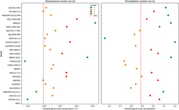
Figure 1 shows the clustering results for both variables, with models ordered by their climatological temperature value so that cross-variable cluster shifts are immediately visible. Temperature exhibits moderate separation (silhouette 0.649), while precipitation displays greater overlap across clusters (silhouette 0.569). This difference likely reflects the higher variability and intermittency of precipitation, but we emphasize that the resulting clusters should be interpreted as approximate groupings rather than sharply separated categories.
Clustering of CMIP6 models based on climatological mean temperature (left) and precipitation (right), using
$ k $
 -means with
$ k=4 $
-means with
$ k=4 $
 . Models are ordered by their climatological temperature value on the shared y-axis, so that color changes at the same y-position (between the two panels) indicate that a model’s cluster assignment differs between the two variables. The red dashed line indicates the ERA5 climatological mean. Colors indicate cluster membership (consistent with all subsequent figures).
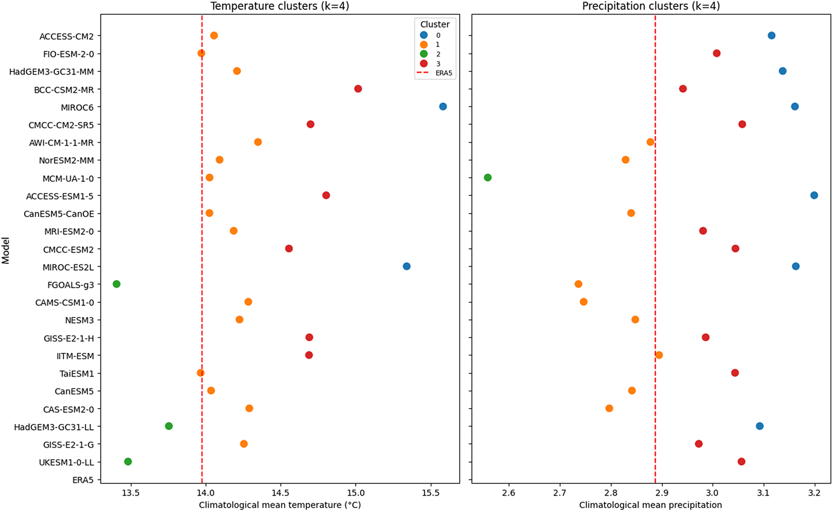
Figure 1. Long description
A two-panel scatter plot compares C M I P 6 models. The shared y-axis lists 25 models from top to bottom, starting with A C C E S S - C M 2 and ending with E R A 5.
Left Panel: Temperature clusters k equals 4. The x-axis represents Climatological mean temperature in degrees Celsius, ranging from 13.5 to 15.5. A red dashed vertical line marks the E R A 5 mean at 14.0. Data points are colored by cluster: blue (0), orange (1), green (2), and red (3). Most models cluster between 14.0 and 15.0 degrees Celsius. F G O A L S - g 3 and U K E S M 1 - 0 - L L are outliers on the lower end, colored green.
Right Panel: Precipitation clusters k equals 4. The x-axis represents Climatological mean precipitation, ranging from 2.6 to 3.2. The red dashed E R A 5 reference line is at approximately 2.88. Cluster colors remain consistent with the left panel. M C M - U A - 1 - 0 is a significant outlier on the low end, colored green.
Horizontal comparison shows that while a model’s position on the y-axis is fixed, its color often changes between panels, indicating different cluster assignments for temperature versus precipitation. For example, M I R O C 6 is in the blue cluster for temperature but remains blue for precipitation, whereas B C C - C S M 2 - M R shifts from red for temperature to red for precipitation.
Importantly, cluster membership depends on the target variable: some models remain grouped across variables, whereas others shift between temperature- and precipitation-based clusters, as is visible in Figure 1 where color changes at the same y-position indicate a cluster shift between the two panels. These patterns highlight that even simple climatological descriptors can capture meaningful differences in model behavior, though they do not directly imply shared model structure or common development lineage.
Preliminary experiments clustering models jointly on standardized temperature and precipitation global means produced broadly similar dominant groupings but with less stable cluster membership across random seeds, suggesting that clustering outcomes are sensitive to feature choice. Richer representations – such as regional averages, multi-decadal statistics, or joint temperature–precipitation features – would likely yield different groupings and are an important direction for future work. In this work, we therefore treat clustering primarily as an exploratory tool to organize model diversity and to provide an interpretive lens for the weight analyses of Section 5.
4. Global prediction performance
We evaluate all ensemble methods on held-out test years (2006–2014) using multiple complementary metrics. Tables 2 and 3 report global results for temperature and precipitation, respectively.
Global prediction performance for near-surface temperature (tas) on the test period 2006–2014

Table 2. Long description
The table consists of seven columns: Method, R M S E, M A E, Corr, N S E, VarRatio, and Skill vs. A M M E.
* Row 1: A M M E. R M S E 0.493, M A E 0.475, Corr 0.996 (bold), N S E 0.873, VarRatio 1.024, Skill vs. A M M E is not applicable.
* Row 2: Ridge. R M S E 0.209, M A E 0.184, Corr 0.996 (bold), N S E 0.977, VarRatio 0.992 (bold), Skill vs. A M M E 0.576.
* Row 3: R F. R M S E 0.225, M A E 0.195, Corr 0.992, N S E 0.974, VarRatio 0.953, Skill vs. A M M E 0.543.
* Row 4: Gating. R M S E 0.196 (bold), M A E 0.169 (bold), Corr 0.996 (bold), N S E 0.980 (bold), VarRatio 0.967, Skill vs. A M M E 0.604 (bold).
Bold values indicate the best performance in each category. For VarRatio, bold indicates the value closest to 1.0. The Gating method shows the best performance across most metrics.
Note. Bold indicates the best value in each column. For VarRatio, bold indicates the value closest to 1.0 (perfect variance calibration). Best Corr is shared by AMME, Ridge, and Gating (all 0.996).
Global precipitation prediction performance on the test period 2006–2014

Table 3. Long description
The table consists of six columns: Method, R M S E, M A E, WetFreq R M S E, Tail R M S E, and Skill vs. A M M E.
* A M M E: R M S E 0.00444, M A E 0.00381, WetFreq R M S E 0.3168, Tail R M S E 0.00684, Skill vs. A M M E is not applicable.
* Ridge: R M S E 0.00243, M A E 0.00198, WetFreq R M S E 0.2165, Tail R M S E 0.00358, Skill vs. A M M E 0.452.
* R F: R M S E 0.00278, M A E 0.00229, WetFreq R M S E 0.2274, Tail R M S E 0.00428, Skill vs. A M M E 0.374.
* Gating: R M S E 0.00218, M A E 0.00176, WetFreq R M S E 0.2093, Tail R M S E 0.00319, Skill vs. A M M E 0.509.
The Gating method shows the best performance across all metrics, indicated by the lowest error values and the highest skill score of 0.509.
Note. Wet-day frequency RMSE measures the error in reproducing the fraction of time steps exceeding 0.1 mm day−1; upper-tail RMSE is restricted to time steps where ERA5 exceeds its 90th percentile. Skill vs. AMME
$ =1-{\mathrm{RMSE}}_{\mathrm{method}}/{\mathrm{RMSE}}_{\mathrm{AMME}} $
 . Bold indicates the best value in each column.
4.1. Temperature
All learning-based methods outperform AMME for global mean temperature (Table 2). Ridge reduces RMSE by more than half relative to AMME, and RF also yields substantial improvement. The gating mixture achieves the best overall performance, with the lowest RMSE (0.196) and highest NSE (0.980). Correlations with ERA5 remain very high across methods, indicating that improvements reflect better tracking of temporal variability rather than simple variance rescaling.
To confirm that these rankings are not artifacts of a single training run, we repeated the experiment with
$ n=10 $
 different random seeds for the RF (Ridge is deterministic given a fixed training set). Table 4 reports mean RMSE and standard deviation across seeds. The standard deviation is near zero for all methods (Ridge: 0.000, RF: 0.002, Gating: 0.001), confirming that the ranking Gating > Ridge > RF > AMME is stable and not attributable to random variation in tree construction.
Stability of global temperature RMSE across
$ n=10 $
 random seeds

Table 4. Long description
The table consists of four columns and three rows.
Column headers from left to right are:
- Empty cell for row labels
- Ridge
- R F
- Gating
Row 1, Mean R M S E:
- Ridge: 0.209
- R F: 0.227
- Gating: 0.196
Row 2, Std R M S E:
- Ridge: 0.000
- R F: 0.002
- Gating: 0.001
A note below the table states that Ridge is deterministic with a standard deviation of 0, and the near-zero standard deviations confirm that the method ranking is not due to random variation.
Note. Ridge is deterministic (std = 0). The near-zero standard deviations confirm that the method ranking is not attributable to random variation.
4.2. Precipitation
For precipitation, we report distribution-aware skill using RMSE, wet-day frequency RMSE, and upper-tail RMSE (Table 3). All learning-based approaches improve over AMME across these metrics. Ridge provides strong gains relative to AMME, while RF improves less consistently. The gating mixture yields the best overall performance globally, improving not only mean error but also wet-day frequency and tail behavior. Compared to temperature, precipitation gains are smaller and more sensitive to method choice, consistent with higher intermittency and noise in the precipitation field.
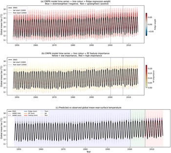
Figure 2 provides a qualitative illustration of the test-period performance. Panel (a) shows all 25 CMIP6 model time series color coded by Ridge regression weight: the most-trusted models (red) track ERA5 closely, while less-trusted models (pale/blue) deviate more. Panel (b) uses the same time series but codes color by RF importance, revealing which models the nonlinear learner relies on most. Panel (c) compares predicted vs. observed global mean temperature for all four methods on the test period (2006–2014): all learning-based methods closely track ERA5, while AMME shows a systematic warm bias reflecting the multi-model mean offset.
Global mean near-surface temperature time series and test-period comparison. (a) All 25 CMIP6 model time series color coded by normalized Ridge regression weight: red indicates high positive weight, blue indicates negative or near-zero weight. ERA5 is shown in black. Training/validation/test periods are delineated by vertical dashed lines. (b) Same time series color coded by RF variable importance (yellow = low, red = high). (c) Predicted vs. observed global mean temperature for AMME (dashed pink) and Gating (solid red) on the test period 2006–2014. Ridge and Gating closely track ERA5, while AMME exhibits a systematic warm bias.
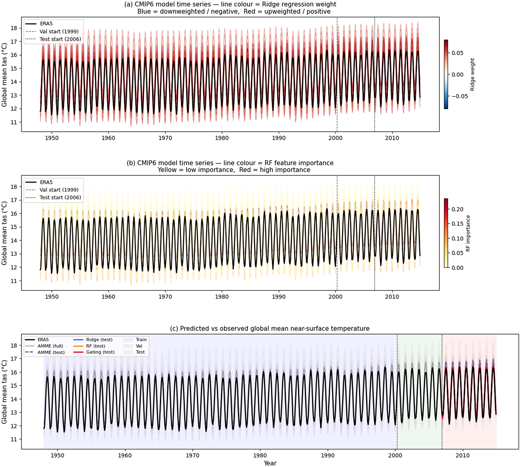
Figure 2. Long description
A multi-panel figure with three vertically stacked line graphs. All panels share a common Y-axis labeled Global mean tas in degrees Celsius, ranging from 11 to 18, and an X-axis representing years from 1950 to 2014.
Panel a displays C M I P 6 model time series color-coded by Ridge regression weight. A vertical dashed line at 1999 marks the Val start and a dotted line at 2006 marks the Test start. High positive weights are shown in red, while negative or near-zero weights are in blue. A thick black line represents E R A 5 data, which oscillates seasonally between 12 and 16 degrees Celsius. A color bar on the right indicates Ridge weight from minus 0.05 to 0.05.
Panel b shows the same time series but color-coded by R F feature importance. Yellow indicates low importance and red indicates high importance. The R F importance color bar on the right ranges from 0.00 to 0.20. The seasonal oscillations remain consistent with panel a.
Panel c displays predicted versus observed global mean near-surface temperature. The background is shaded in light blue for Train (1950 to 1999), light green for Val (2000 to 2006), and light red for Test (2007 to 2014). The legend identifies E R A 5 as a solid black line, A M M E full as a solid light purple line, A M M E test as a dashed purple line, Ridge test as a blue line, R F test as an orange line, and Gating test as a solid red line. In the test period, the Gating and Ridge lines closely overlap the E R A 5 black line, while the A M M E lines show a distinct upward shift, indicating a warm bias.
5. Interpretable model weights & gating behavior
While ensemble learning methods improve predictive skill, their scientific value ultimately depends on whether they provide interpretable insight into the role of individual climate models. We therefore analyze the effective weights assigned to each CMIP6 model under Ridge regression and the gating mixture model, and examine how these weights vary across clusters, spatial regions, and seasons.
5.1. Global ridge weights and comparison with RF
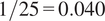
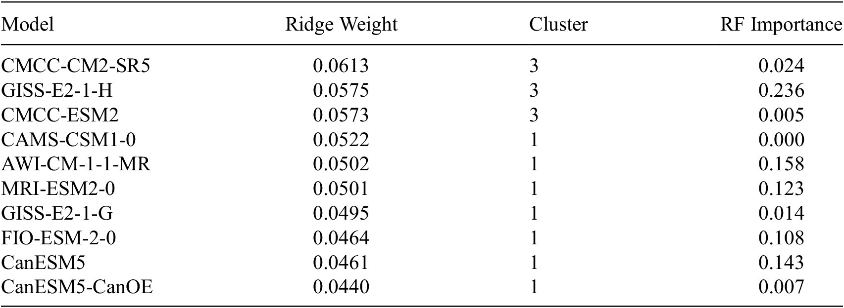
Table 5 lists the ten models receiving the highest global Ridge weights for temperature, together with their RF importance scores. These models contribute heterogeneously to the ensemble prediction: the top-weighted models receive approximately
$ 1.5\times $
 the uniform AMME weight (
$ 1/25=0.040 $
the uniform AMME weight (
$ 1/25=0.040 $
 ), while the lowest-weighted models receive correspondingly less. The degree of concentration is controlled by the
$ {\mathrm{\ell}}_2 $
), while the lowest-weighted models receive correspondingly less. The degree of concentration is controlled by the
$ {\mathrm{\ell}}_2 $
 regularization strength: larger
$ \alpha $
regularization strength: larger
$ \alpha $
 pushes weights toward uniformity, while smaller
$ \alpha $
pushes weights toward uniformity, while smaller
$ \alpha $
 allows greater differentiation.
Top ten CMIP6 models by global Ridge weight for temperature, together with their cluster assignment (consistent with the fixed-seed clustering reported in Section 3)
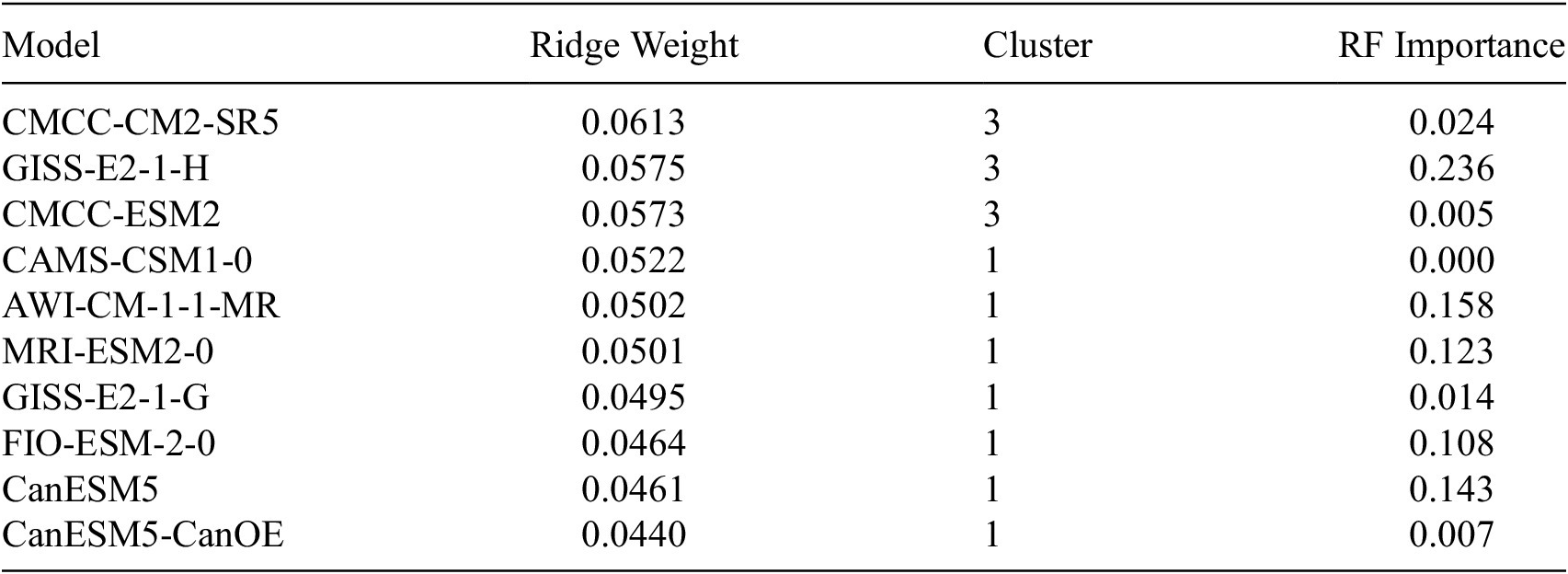
Table 5. Long description
The table consists of four columns: Model, Ridge Weight, Cluster, and R F Importance. The data is as follows:
* C M C C-C M 2-S R 5: Ridge Weight 0.0613, Cluster 3, R F Importance 0.024.
* G I S S-E 2-1-H: Ridge Weight 0.0575, Cluster 3, R F Importance 0.236.
* C M C C-E S M 2: Ridge Weight 0.0573, Cluster 3, R F Importance 0.005.
* C A M S-C S M 1-0: Ridge Weight 0.0522, Cluster 1, R F Importance 0.000.
* A W I-C M-1-1-M R: Ridge Weight 0.0502, Cluster 1, R F Importance 0.158.
* M R I-E S M 2-0: Ridge Weight 0.0501, Cluster 1, R F Importance 0.123.
* G I S S-E 2-1-G: Ridge Weight 0.0495, Cluster 1, R F Importance 0.014.
* F I O-E S M-2-0: Ridge Weight 0.0464, Cluster 1, R F Importance 0.108.
* CanESM5: Ridge Weight 0.0461, Cluster 1, R F Importance 0.143.
* CanESM5-CanOE: Ridge Weight 0.0440, Cluster 1, R F Importance 0.007.
Note. The rightmost column shows the corresponding RF importance score for comparison.
Notably, the highest-weighted models are concentrated within Clusters 1 and 3 for Ridge, suggesting that Ridge regression preferentially amplifies specific model families rather than uniformly redistributing trust across the ensemble.
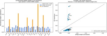
Comparing Ridge weights with RF importances (Table 5 and Figure 3) reveals partial but imperfect agreement (Pearson
$ r=0.52 $
 ). Six models receive substantially higher RF importance than Ridge weight: GISS-E2-1-H (RF: 0.236 vs. Ridge: 0.050), AWI-CM-1-1-MR (0.158 vs. 0.050), CanESM5 (0.143 vs. 0.046), MRI-ESM2–0 (0.123 vs. 0.050), FIO-ESM-2-0 (0.108 vs. 0.048), and FGOALS-g3 (0.106 vs. 0.044). These models appear to carry nonlinear information that the RF can exploit but that Ridge, as a globally linear model, cannot fully capture. Conversely, many models receive higher Ridge weight than RF importance, reflecting the regularized distribution of weights that Ridge enforces.
(a) Normalized Ridge regression weights (blue) and RF variable importances (orange) for all 25 CMIP6 models, sorted by Ridge weight. The dashed gray line shows the uniform AMME weight (1/25). (b) Scatter of normalized Ridge weight vs. RF importance per model (Pearson
$ r=0.52 $
 ). Models above the diagonal are more trusted by RF than Ridge; the six models with RF importance
$ >2\times $
). Models above the diagonal are more trusted by RF than Ridge; the six models with RF importance
$ >2\times $
 Ridge weight are labeled. The partial agreement indicates that the two learners identify overlapping but non-identical sets of informative models.
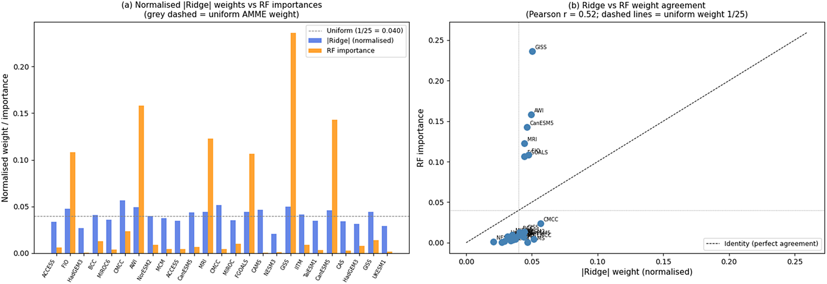
Figure 3. Long description
Panel A is a bar chart titled Normalised Ridge weights versus R F importances. The y-axis represents Normalised weight or importance from 0.00 to 0.25. The x-axis lists 25 climate models. Blue bars represent Ridge weights, which remain relatively stable near the dashed gray uniform A M M E weight line at 0.040. Orange bars represent R F importance, showing high variability with significant peaks for models like F I O, A W I, M R I, C A M S, I I T M, and C A S.
Panel B is a scatter plot titled Ridge versus R F weight agreement with a Pearson r of 0.52. The x-axis is the absolute Ridge weight (normalised) and the y-axis is R F importance, both ranging from 0.00 to 0.25. A dashed diagonal line represents perfect agreement. Most models cluster in the bottom-left corner below the 0.05 mark on both axes. Six outlier models are labeled high above the diagonal, indicating much higher R F importance than Ridge weight: G I S S, A W I, Can E S M 5, M R I, F I O, and F G O A L S. Horizontal and vertical gray lines intersect at the 0.04 uniform weight mark.
Figure 3 illustrates this comparison across all 25 models. Panel (a) shows normalized Ridge weights and RF importances as a grouped bar chart, with the uniform AMME baseline shown as a dashed line. Panel (b) shows a scatter plot of the two quantities; models above the identity line are RF-preferred, while models below are Ridge-preferred. The six strongly RF-preferred models cluster in the upper-left region. The partial agreement (
$ r=0.52 $
 ) is interpreted in Section 5.2: the gating exploits both sets of signals by adaptively blending the two learners.
5.2. Spatial structure of gating and model dominance
To examine how the gating ensemble redistributes trust across space, we analyze the dominant-cluster and dominant-model at each grid cell, based on the mean per-model gating weight (i.e., the average absolute weight per model within each cluster, rather than the sum, to avoid bias toward whichever cluster has the most members).
For spatial reference, we define three large-scale regions: the Tropics (
$ 30{}^{\circ} $
 S–
$ 30{}^{\circ} $
S–
$ 30{}^{\circ} $
 N), Northern Hemisphere mid-latitudes (
$ 30{}^{\circ} $
N), Northern Hemisphere mid-latitudes (
$ 30{}^{\circ} $
 N–
$ 60{}^{\circ} $
N–
$ 60{}^{\circ} $
 N), and the Arctic (
$ 60{}^{\circ} $
N), and the Arctic (
$ 60{}^{\circ} $
 N–
$ 90{}^{\circ} $
N–
$ 90{}^{\circ} $
 N). The mean gating skill improvement over AMME is
$ +0.418 $
N). The mean gating skill improvement over AMME is
$ +0.418 $
 in the Tropics,
$ +0.148 $
in the Tropics,
$ +0.148 $
 in NH mid-latitudes,
$ +0.319 $
in NH mid-latitudes,
$ +0.319 $
 in the Southern Hemisphere mid-latitudes,
$ +0.298 $
in the Southern Hemisphere mid-latitudes,
$ +0.298 $
 in the Arctic, and
$ +0.294 $
in the Arctic, and
$ +0.294 $
 in the Antarctic.
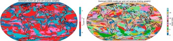
The left panel of Figure 4 shows the dominant-model cluster per grid cell. Clear large-scale spatial organization emerges, with distinct cluster regimes in the tropics, mid-latitudes, and high-latitude oceans. Cluster 0 (MIROC models) dominates parts of the tropical and subtropical oceans; Cluster 3 (CMCC, GISS-H, ACCESS-ESM1–5 group) is preferred over continental interiors and parts of the Southern Ocean; Cluster 1 (the large 14-member group) dominates high-latitude regions. These spatial patterns are broadly consistent with known dynamical differences among climate model families: for example, the MIROC models are known for distinctive SST biases in the tropical Pacific, while the CMCC and GISS families differ in aerosol forcing and ocean heat uptake representations (Sanderson et al., Reference Sanderson, Knutti and Caldwell2015; Knutti et al., Reference Knutti, Sedláček, Sanderson, Lorenz, Fischer and Eyring2017). The right panel of Figure 4 shows the dominant individual CMIP6 model per grid cell. Rather than a single model dominating globally, the gating ensemble exhibits strong spatial diversity, with different models preferred in different regions.
(Left) Dominant CMIP6 model cluster per grid cell, defined by the cluster whose models receive the highest mean per-model gating weight. (Right) Dominant individual CMIP6 model per grid cell, defined by the model with the maximum average gating weight. Results show strong spatial structure in ensemble trust, with different clusters and models preferred across distinct dynamical regimes. Cluster IDs: 0 = MIROC family (2 models), 1 = large mid-bias group (14 models), 2 = HadGEM–UKESM family (3 models), 3 = CMCC–GISS-H group (6 models).
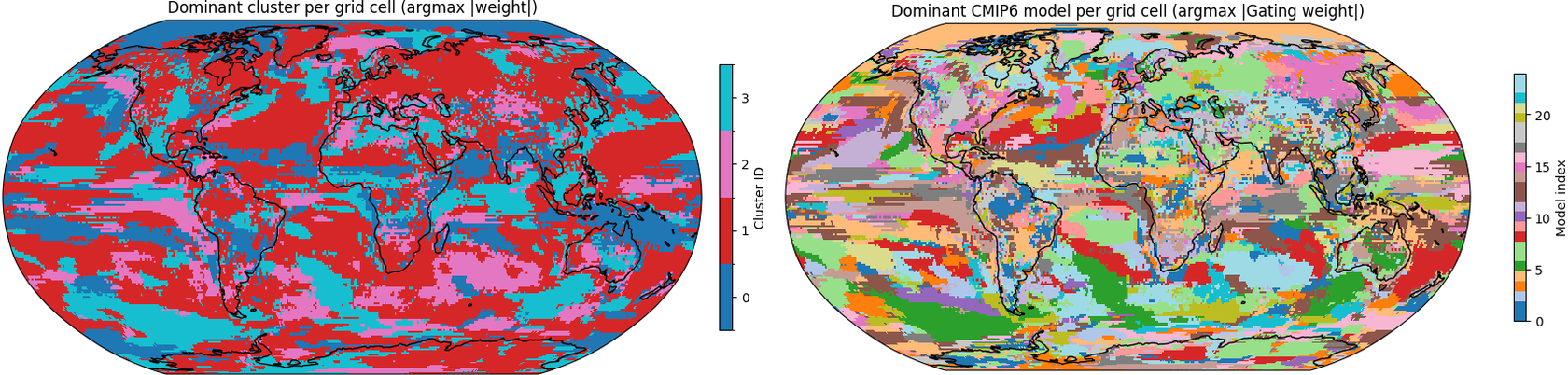
Figure 4. Long description
A two-panel visualization of global climate model distribution.
Left Panel: Dominant cluster per grid cell (argmax |weight|).
* The map uses four distinct colors to represent Cluster I D values from 0 to 3.
* Red (Cluster 1) is the most widespread, covering most of North America, Eurasia, North Africa, and the Southern Ocean.
* Blue (Cluster 0) is concentrated in the tropical Pacific and parts of the Southern Hemisphere.
* Pink (Cluster 2) appears in the South Atlantic, Indian Ocean, and parts of Antarctica.
* Cyan (Cluster 3) is scattered across the North Pacific and high-latitude regions.
* A vertical color bar to the right labels the Cluster I D from 0 (bottom) to 3 (top).
Right Panel: Dominant C M I P 6 model per grid cell (argmax |Gating weight|).
* This map features a highly fragmented, multi-colored mosaic representing individual models.
* Large contiguous blocks are visible in the Southern Ocean (green and purple), the Sahara (light green), and the North Atlantic (red).
* The tropical regions show high variability with small, pixelated color changes.
* A vertical color bar to the right, titled Model index, ranges from 0 to over 20, using a diverse categorical color palette to identify specific models.
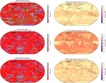
To understand how gating relates to its two components, Figure 5 shows dominant-cluster maps and trust entropy maps for Ridge, RF, and Gating side by side. Ridge produces a spatially smooth, multi-cluster pattern (mean
$ {N}_{\mathrm{eff}}=21.1 $
 ), while RF is more concentrated (mean
$ {N}_{\mathrm{eff}}=13.4 $
), while RF is more concentrated (mean
$ {N}_{\mathrm{eff}}=13.4 $
 ), reflecting the implicit feature selection of tree-based methods. Gating achieves an intermediate effective ensemble size (
$ {N}_{\mathrm{eff}}=19.5 $
), reflecting the implicit feature selection of tree-based methods. Gating achieves an intermediate effective ensemble size (
$ {N}_{\mathrm{eff}}=19.5 $
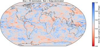
 ), broadly following the Ridge spatial pattern but selectively concentrating trust in regions where RF’s nonlinear predictions are locally superior – consistent with the gating mechanism blending both learners. The spatial distribution of the per-pixel mean gate value
$ \overline{g} $
), broadly following the Ridge spatial pattern but selectively concentrating trust in regions where RF’s nonlinear predictions are locally superior – consistent with the gating mechanism blending both learners. The spatial distribution of the per-pixel mean gate value
$ \overline{g} $
 (Figure 6) confirms this: 55% of pixels are Ridge-dominated (
$ \overline{g}>0.5 $
(Figure 6) confirms this: 55% of pixels are Ridge-dominated (
$ \overline{g}>0.5 $
 ) and 45% are RF-dominated (
$ \overline{g}<0.5 $
) and 45% are RF-dominated (
$ \overline{g}<0.5 $
 ), with RF dominance concentrated in tropical and Southern Ocean regions that also exhibit the strongest skill improvement.
Dominant cluster (left column) and trust entropy (right column) for Ridge (top), RF (middle), and Gating (bottom). Ridge maintains high entropy (mean
$ {N}_{\mathrm{eff}}=21.1 $
 ) with a spatially smooth multi-cluster pattern. RF is more concentrated (mean
$ {N}_{\mathrm{eff}}=13.4 $
) with a spatially smooth multi-cluster pattern. RF is more concentrated (mean
$ {N}_{\mathrm{eff}}=13.4 $
 ), with stronger Cluster-0 (MIROC) dominance in the tropics. Gating achieves an intermediate
$ {N}_{\mathrm{eff}}=19.5 $
), with stronger Cluster-0 (MIROC) dominance in the tropics. Gating achieves an intermediate
$ {N}_{\mathrm{eff}}=19.5 $
 , selectively concentrating trust in regions where RF’s nonlinear predictions are locally superior.
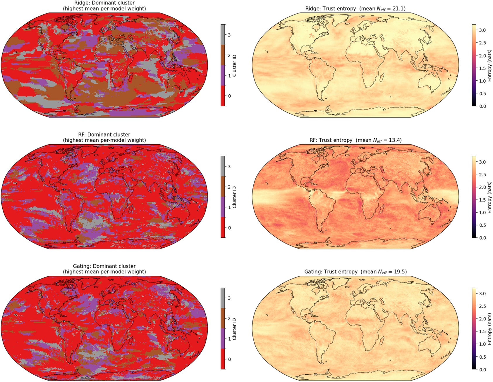
Figure 5. Long description
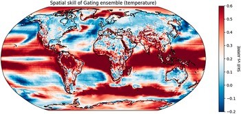
A Robinson projection world map titled Spatial skill of Gating ensemble temperature. The map uses a diverging color scale to represent Skill vs A M M E.
* The color scale on the right ranges from negative 0.2 in dark blue to 0.6 in dark red.
* High skill values between 0.4 and 0.6 are concentrated in the tropical oceans, particularly across the central Pacific, the tropical Atlantic, and the Indian Ocean.
* High skill is also visible over large landmasses including central and southern Africa, South America, and parts of South Asia.
* Low or negative skill values between negative 0.2 and 0.1 are shown in light to dark blue, appearing predominantly in the high latitudes of the Northern Hemisphere, including the Arctic Ocean, northern North America, and northern Eurasia.
* Australia and the Southern Ocean show a mix of moderate skill in light red and low skill in light blue.
* The transition between high and low skill regions is granular, with a pixelated texture across most continental regions.
Spatial distribution of the time-mean gate value
$ \overline{g} $
 (per pixel). Red (
$ \overline{g} $
(per pixel). Red (
$ \overline{g} $
 near 1) indicates Ridge-dominated pixels; blue (
$ \overline{g} $
near 1) indicates Ridge-dominated pixels; blue (
$ \overline{g} $
 near 0) indicates RF-dominated pixels. Overall, 55% of pixels are Ridge-dominated and 45% are RF-dominated. RF dominance is concentrated in tropical oceans and the Southern Ocean, which also exhibit the strongest skill improvement relative to AMME (Figure 7).
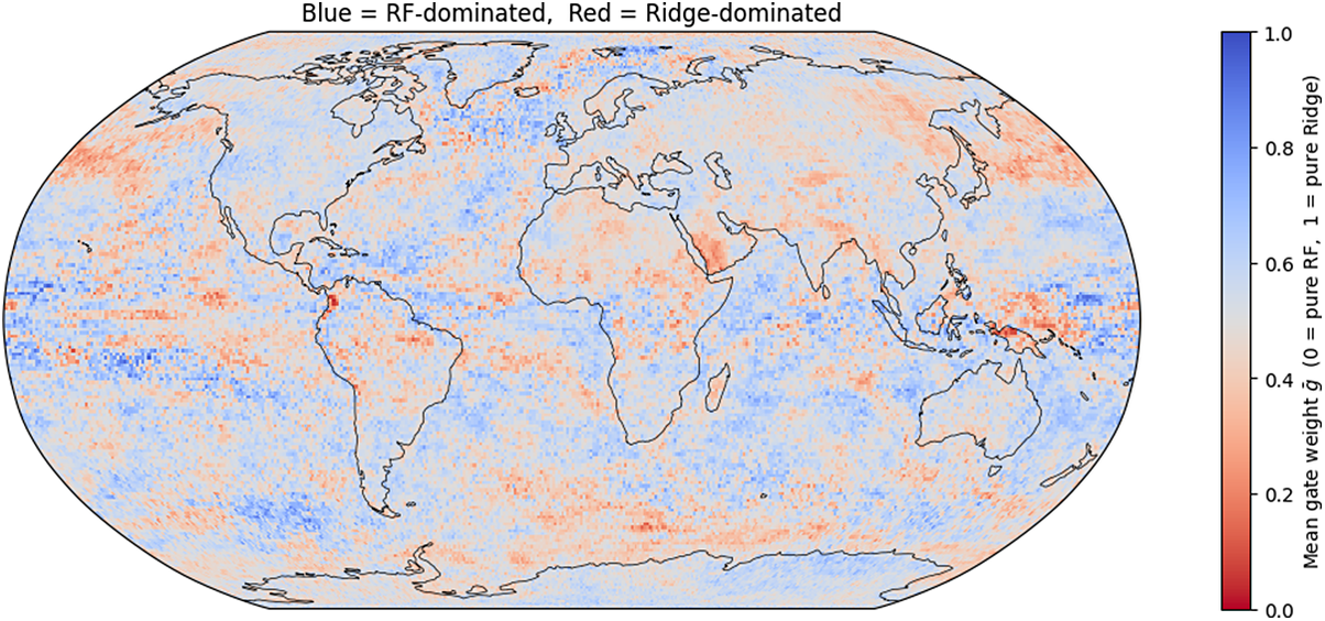
Figure 6. Long description
The grid consists of three rows representing different methods: Ridge at the top, R F in the middle, and Gating at the bottom.
Left Column: Dominant cluster maps. These maps use a discrete color scale for Cluster I D from 0 to 3.
* Row 1 (Ridge): Shows a high concentration of red (Cluster 0) and brown (Cluster 2) across the globe.
* Row 2 (R F): Dominated heavily by red (Cluster 0) across almost all ocean and land masses, with small patches of purple (Cluster 1) and grey (Cluster 3).
* Row 3 (Gating): Similar to R F but with slightly more purple (Cluster 1) and grey (Cluster 3) distribution in the Southern Hemisphere and tropical regions.
Right Column: Trust entropy maps. These maps use a continuous diverging colormap from 0.0 to 3.0 nats.
* Row 1 (Ridge): Mean N sub eff equals 21.1. The map is mostly light yellow, indicating low entropy, with slightly darker shades in the Southern Ocean.
* Row 2 (R F): Mean N sub eff equals 13.4. This map shows significantly higher entropy (darker orange and red hues) across the tropical oceans and Southern Hemisphere compared to the other methods.
* Row 3 (Gating): Mean N sub eff equals 19.5. The entropy levels are lower than R F, appearing mostly light yellow with moderate orange shading concentrated in the tropical Pacific and Indian Oceans.
Figure 7 shows the spatial distribution of skill improvement of the gating ensemble relative to AMME for near-surface temperature. Large contiguous regions exhibit substantial positive skill, particularly over tropical oceans, the Southern Ocean, and parts of the Indian Ocean basin. These regions correspond to areas of strong model disagreement and known systematic biases in coupled climate models, suggesting that gating is most effective where ensemble diversity is high and model errors are structured rather than random. Conversely, regions with weak or near-zero skill gains are primarily located over continental interiors and high-latitude land areas, where internal variability dominates and cross-model differences are less informative. This spatial pattern indicates that gating does not uniformly improve predictions everywhere but selectively enhances skill in regions where ensemble learning is epistemically meaningful.
Spatial distribution of skill improvement of the gating ensemble relative to AMME for near-surface temperature (test period 2006–2014). The diverging colormap is centered at zero (white), with red indicating improvement and blue indicating degradation relative to AMME. Positive values indicate regions where gating reduces RMSE compared to the arithmetic ensemble. Strong improvements occur over tropical oceans and parts of the Southern Hemisphere; small degradations occur over some continental interiors and high-latitude land areas.
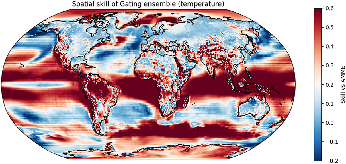
Figure 7. Long description
A world map in a Robinson-style projection displays mean gate weight g-bar per pixel. A color scale on the right ranges from 0.0 in dark red to 1.0 in dark blue.
* The scale indicates that 0 equals pure R F and 1 equals pure Ridge.
* Blue pixels, representing R F dominance, are heavily concentrated in the Southern Ocean surrounding Antarctica and across the tropical Pacific and Indian Oceans.
* Red pixels, representing Ridge dominance, are more prevalent over landmasses and in the high Northern latitudes, particularly the North Atlantic and Arctic regions.
* The transition zones between these regions appear in light white or pale orange, indicating a mix of both models.
* A title at the top explicitly states Blue equals R F-dominated and Red equals Ridge-dominated.
Compared to traditional performance-based weighting schemes – such as scalar skill-based weighting (Knutti et al., Reference Knutti, Sedláček, Sanderson, Lorenz, Fischer and Eyring2017) or the ClimWIP approach (Sanderson et al., Reference Sanderson, Knutti and Caldwell2015), which assign globally uniform scalar weights – the gating mechanism operates at the pixel level and is time-varying, allowing trust to be concentrated only where and when a sub-model is locally superior. The
$ {\mathrm{\ell}}_2 $
 regularization in Ridge explains why that component maintains high entropy (many models contribute); the tree-based selection of RF explains its lower entropy; and gating mediates between these extremes.
5.3. Trust dispersion and effective ensemble size
To quantify how concentrated or distributed model trust is under the gating ensemble, we compute the entropy of the gating weights at each grid cell (Section 2.5). Higher entropy indicates more evenly distributed trust across models, while lower entropy indicates strong concentration on a small number of models.
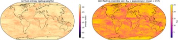
Figure 8 shows the spatial distribution of trust entropy for the gating ensemble. Most regions exhibit relatively high entropy, corresponding to a mean effective ensemble size of
$ {N}_{\mathrm{eff}}=19.5 $
 models. For comparison, Ridge yields
$ {N}_{\mathrm{eff}}=21.1 $
models. For comparison, Ridge yields
$ {N}_{\mathrm{eff}}=21.1 $
 and RF yields
$ {N}_{\mathrm{eff}}=13.4 $
and RF yields
$ {N}_{\mathrm{eff}}=13.4 $
 (see also Figure 5). This indicates that, despite spatially varying dominance patterns, gating generally maintains a broad ensemble rather than collapsing to a few preferred models.
Spatial distribution of trust dispersion under the Gating ensemble, measured as (a) trust entropy
$ H $
 and (b) effective ensemble size
$ {N}_{\mathrm{eff}}=\exp (H) $
and (b) effective ensemble size
$ {N}_{\mathrm{eff}}=\exp (H) $
 [mean
$ =19.5 $
[mean
$ =19.5 $
 models]. Higher values indicate more evenly distributed trust (larger effective ensemble size), while lower values indicate strong concentration on a small subset of models. For comparison, Ridge yields mean
$ {N}_{\mathrm{eff}}=21.1 $
models]. Higher values indicate more evenly distributed trust (larger effective ensemble size), while lower values indicate strong concentration on a small subset of models. For comparison, Ridge yields mean
$ {N}_{\mathrm{eff}}=21.1 $
 and RF yields mean
$ {N}_{\mathrm{eff}}=13.4 $
and RF yields mean
$ {N}_{\mathrm{eff}}=13.4 $
 ; see Figure 5 for side-by-side entropy maps of all three methods.
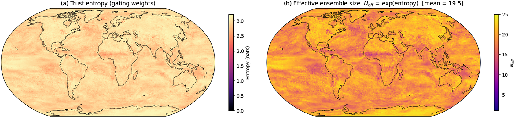
Figure 8. Long description
Two side-by-side global maps using a Robinson projection.
Panel a is titled Trust entropy gating weights. It displays a heat map where values are measured in nats. The color scale on the right ranges from 0.0 black to 3.0 light yellow. The map is predominantly light yellow and pale orange, indicating high entropy across most of the globe, with slightly lower values appearing as darker orange patches in the Southern Ocean and parts of the North Atlantic.
Panel b is titled Effective ensemble size N sub eff = exp entropy mean = 19.5. The color scale on the right ranges from 0 to 25, with dark purple representing low values and bright yellow representing high values. The map shows a more heterogeneous distribution than panel a. High values near 20 to 25 are concentrated in the tropical regions and mid-latitudes of both the Northern and Southern Hemispheres. Lower values, indicated by purple and dark pink patches, are visible in the North Atlantic, the Southern Ocean near Antarctica, and parts of the South Pacific, indicating a higher concentration of trust on fewer models in these specific geographical zones.
Regions with lower entropy appear primarily in parts of the tropical oceans and the Southern Ocean, where a small subset of models consistently outperforms others. These regions also correspond to areas of particularly strong skill improvement under gating (Figure 7), suggesting that localized trust concentration is associated with genuine predictive advantage.
Taken together, these results demonstrate that gating produces a structured redistribution of trust: locally selective where strong signals exist, but globally conservative in preserving ensemble diversity. This behavior supports the interpretation of gating as a principled trust reallocation mechanism rather than an aggressive model selection procedure.
5.4. Temporal and seasonal behavior of the gate
To assess the temporal consistency of the gating weights, Figure 9 shows the gate value
$ {g}_t $
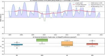
 over the test period 2006–2014 together with a 12-month rolling mean and a per-season breakdown. The gate is Ridge-dominated for 92% of monthly time steps (global mean
$ \overline{g}=0.685 $
over the test period 2006–2014 together with a 12-month rolling mean and a per-season breakdown. The gate is Ridge-dominated for 92% of monthly time steps (global mean
$ \overline{g}=0.685 $
 ) but exhibits meaningful seasonal modulation. MAM (spring) has the highest mean gate value (
$ {\overline{g}}_{\mathrm{MAM}}=0.873 $
) but exhibits meaningful seasonal modulation. MAM (spring) has the highest mean gate value (
$ {\overline{g}}_{\mathrm{MAM}}=0.873 $
 , almost entirely Ridge-dominated), while DJF (winter) has the lowest (
$ {\overline{g}}_{\mathrm{DJF}}=0.592 $
, almost entirely Ridge-dominated), while DJF (winter) has the lowest (
$ {\overline{g}}_{\mathrm{DJF}}=0.592 $
 ), with JJA and SON at intermediate values (0.638 and 0.639, respectively). This pattern suggests that the global mean relationship between CMIP6 models and ERA5 is more linear in spring – when ensemble spread may be dominated by systematic rather than nonlinear biases – and that the RF nonlinearity contributes more in winter. We note that this temporal gate operates on the global mean signal; spatial variation of
$ \overline{g} $
), with JJA and SON at intermediate values (0.638 and 0.639, respectively). This pattern suggests that the global mean relationship between CMIP6 models and ERA5 is more linear in spring – when ensemble spread may be dominated by systematic rather than nonlinear biases – and that the RF nonlinearity contributes more in winter. We note that this temporal gate operates on the global mean signal; spatial variation of
$ \overline{g} $
 is shown in Figure 6. Seasonal effects on the spatial gating weights are a natural direction for future work.
(a) Temporal evolution of the global gating weight
$ {g}_t $
 over the test period 2006–2014. Blue shading indicates Ridge-dominated months (
$ {g}_t>0.5 $
over the test period 2006–2014. Blue shading indicates Ridge-dominated months (
$ {g}_t>0.5 $
 ); yellow shading indicates RF-dominated months (
$ {g}_t<0.5 $
); yellow shading indicates RF-dominated months (
$ {g}_t<0.5 $
 ). The red curve shows a 12-month rolling mean; the dotted horizontal line shows the global mean
$ \overline{g}=0.685 $
). The red curve shows a 12-month rolling mean; the dotted horizontal line shows the global mean
$ \overline{g}=0.685 $
 . (b) Seasonal distribution of
$ {g}_t $
. (b) Seasonal distribution of
$ {g}_t $
 : MAM is strongly Ridge-dominated (mean 0.873), while DJF shows the greatest RF contribution (mean 0.592). Boxplots show the interquartile range and outliers across individual months within each season.
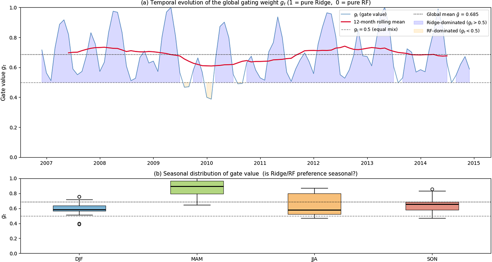
Figure 9. Long description
Panel a is a line graph titled Temporal evolution of the global gating weight g sub t. The y-axis is Gate value g sub t ranging from 0.0 to 1.0. The x-axis shows years from 2007 to 2015. A blue line fluctuates between 0.4 and 1.0. Areas where g sub t is greater than 0.5 are shaded blue, indicating Ridge-dominated months. Small areas where g sub t is less than 0.5 are shaded yellow, indicating R F-dominated months. A red curve represents a 12-month rolling mean, staying relatively stable between 0.6 and 0.8. A dotted horizontal line marks the global mean g-bar equals 0.685, and a dashed line marks the 0.5 equal mix threshold.
Panel b is a boxplot titled Seasonal distribution of gate value. The y-axis is g sub t and the x-axis lists four seasons.
- D J F is blue with a median near 0.6 and two outliers.
- M A M is green with the highest median near 0.9.
- J J A is orange with a median near 0.6 and a wide interquartile range.
- S O N is red with a median near 0.65 and one outlier.
The global mean and 0.5 threshold lines from panel a are extended across these boxplots.
6. Conclusion
This paper presented an interpretable ensemble learning framework that improves prediction while making the contributions of individual CMIP6 models explicit. We first clarified that the clustering analysis is an exploratory organizational tool rather than a definitive characterization of model structural similarity:
$ k $
 -means on global climatological means provides a coarse, interpretable partition that can be directly related to how ensemble learning redistributes weights but does not recover code-lineage or parameterization relationships. We showed that CMIP6 exhibits structured diversity: temperature supports moderate clustering and precipitation displays greater overlap. Building on this, we compared four ensemble strategies against ERA5 using a time-ordered split. For near-surface temperature, all learning-based methods substantially outperformed AMME, with the gating mixture achieving the best performance; stability analysis over ten random seeds confirms these rankings are robust. For precipitation, distribution-aware evaluation showed that learning-based ensembles improve not only mean error but also wet-day frequency and tail behavior, with gating again yielding the strongest global results.
Crucially, improvements arise from structured reallocation of trust rather than global selection of a single model. Spatial analyses reveal that gating concentrates weights only where doing so provides clear benefit, while maintaining a broad effective ensemble (
$ {N}_{\mathrm{eff}}\approx 19.5 $
 ) elsewhere. A comparison of Ridge, RF, and gating spatial weight patterns shows that RF is more concentrated (
$ {N}_{\mathrm{eff}}=13.4 $
) elsewhere. A comparison of Ridge, RF, and gating spatial weight patterns shows that RF is more concentrated (
$ {N}_{\mathrm{eff}}=13.4 $
 ) while Ridge is more distributed (
$ {N}_{\mathrm{eff}}=21.1 $
) while Ridge is more distributed (
$ {N}_{\mathrm{eff}}=21.1 $
 ); gating mediates between these extremes, exploiting both the linear regularization of Ridge and the nonlinear feature selection of RF. Temporal analysis of the gate shows meaningful seasonal variation, with Ridge-dominated behavior in spring and greater RF contribution in winter, though causal attribution of this pattern to specific physical processes remains an open question.
These results suggest a practical middle ground between model democracy and aggressive model selection: ensemble learning can improve skill while remaining transparent and auditable. Future work should extend this approach to richer model descriptors (e.g., regional statistics, multi-decadal trends), uncertainty-aware objectives, sparse weighting schemes (e.g., LASSO), joint multivariate learning across temperature and precipitation, and additional observational products, and should assess whether seasonal and regional patterns in gating weights can be attributed to specific physical mechanisms in the underlying models.
Acknowledgments
We acknowledge the World Climate Research Programme (WCRP), which, through its Coupled Model Intercomparison Project (CMIP), coordinated the CMIP6 experiments used in this study. We thank the climate modeling groups for producing and making their model outputs publicly available, the Earth System Grid Federation (ESGF) for archiving and distributing CMIP6 data, and the European Centre for Medium-Range Weather Forecasts (ECMWF) for providing the ERA5 reanalysis dataset.
Author contribution
Conceptualization: S.W. Methodology: S.W. Software: S.E. Formal analysis: S.W. Data curation: S.W. Visualization: S.W. Writing – original draft preparation: S.W. Writing – review and editing: S.E., S.W. Supervision: S.E. All authors discussed the results and approved the final manuscript. All authors approved the final submitted draft.
Competing interests
The author(s) declare none.
Data availability statement
CMIP6 model outputs are publicly available through the Earth System Grid Federation (ESGF) data portals (https://esgf-node.llnl.gov/). ERA5 reanalysis data are available from the Copernicus Climate Data Store (https://cds.climate.copernicus.eu/). The analysis code and processed scripts used to reproduce all results and figures in this study are openly available on GitHub and archived on Zenodo at https://doi.org/10.5281/zenodo.19433526 under an MIT license.
Ethics statement
This study uses publicly available climate model simulations and reanalysis products and does not involve human participants, animals, or personal data. The research complies with all applicable institutional and international guidelines for the use of publicly available scientific data.
Funding statement
This work was supported by the Canadian Network for Research and Innovation in Machining Technology and the Natural Sciences and Engineering Research Council of Canada (NSERC), grant number RGPIN-202.
Provenance statement
This article is part of the Climate Informatics 2026 proceedings and was accepted in Environmental Data Science on the basis of the Climate Informatics peer review process.


















 Open access

