





Policy Significance Statement
Public employment services increasingly use machine learning tools to predict jobseekers’ risk of long-term unemployment. However, these tools raise concerns about transparency, fairness, and accountability. The present paper demonstrates that transparent (interpretable) machine learning models can predict long-term unemployment almost as well as noninterpretable models. Transparent tools can make employment services more accountable and participatory without sacrificing efficiency. They allow caseworkers and jobseekers to understand and contest predictions, enable policymakers to evaluate the consequences of machine learning tools, and help developers to identify data issues. Using interpretable models may enhance oversight, fairness, and trust in decision-making in public employment services.
1. Introduction
Long-term unemployment (LTU) is a big social challenge, with high costs to both affected jobseekers and the public. To identify jobseekers at risk, public employment services (PESs) increasingly rely on statistical profiling methods to determine jobseekers’ risk of LTU. Statistical profiling promises to make profiling more accurate. Accuracy is sometimes considered to be the most important measure of successful profiling (Desiere et al., Reference Desiere, Langenbucher and Struyven2019), because it may increase the efficiency of activation measures and thus prevent LTU.
Nevertheless, researchers also increasingly recognize that statistical profiling methods may create new problems and exacerbate existing ones. First, statistical profiling may provide unfair or even discriminatory predictions, putting socially salient groups at a disadvantage (Desiere et al., Reference Desiere, Langenbucher and Struyven2019; Allhutter et al., Reference Allhutter, Mager, Cech, Fischer and Grill2020). Second, some profiling methods that use machine learning (ML) methods are considered to be opaque (black-box), meaning that their functioning is hard to understand. Some PESs nevertheless use black-box models (Gallagher and Griffin, Reference Gallagher and Griffin2023) because they promise higher accuracy than alternatives, and accuracy is important for successful profiling. However, black-box models also create problems for key stakeholders: They threaten to sideline PES caseworkers by automating their work. Black-box models also create an accountability gap by not providing jobseekers with a faithful explanation of their unemployment risk. They thereby not only prevent jobseekers from adapting their behavior but also from recourse against predictions and decisions.
Despite these problems, the use of black-box methods—and possible alternatives—in jobseeker profiling remains undertheorized and underexplored. The benefits of transparent models in jobseeker profiling have not been spelled out in the pertinent literature, and their accuracy has not been empirically compared to black-box models using real-life data. Furthermore, the relation between desiderata such as accuracy, interpretability, and fairness has not been sufficiently investigated. For instance, on the one hand, transparent models can make it easier to identify fairness issues; on the other hand, black-box models can also be made to comply with statistical notions of fairness. These desiderata and their associated trade-offs need to be explored so that policymakers can make informed decisions.
This paper presents a first empirical investigation of interpretable statistical profiling. Interpretable models are ML models built to be inherently transparent. Both their general functioning and predictions for individual jobseekers can be understood. Using administrative data from Switzerland, this paper compares opaque and interpretable models, measuring their predictive performance, interpretability, and fairness. It provides a proof-of-concept study that interpretable models trained with administrative data can yield predictive performance only slightly worse than the best black-box models. It establishes the relevance of interpretability to stakeholders (jobseekers, caseworkers, policymakers, model developers) in profiling. It also shows that improving fairness is compatible with interpretable profiling. Interpretable profiling has the potential to increase transparency, accountability, and ultimately trust in employment services. The absolute predictive performance reported in this paper should be interpreted with caution, because the use of administrative data can lead to an overestimation of performance (see Section 3 for discussion).
The paper is structured as follows. Background on LTU profiling and related work, both from the profiling and the ML literature, is presented in Section 2. The stakeholder perspective is also introduced there. Data and methods are introduced in Sections 3 and 4 respectively. Empirical results are given in Section 5. A thorough contextualization of results, with a discussion of limitations and future work, is given in Section 6. The conclusion is given in Section 7.
2. Background and related work
2.1. Prediction of LTU
There are three types of jobseeker profiling for LTU risk: rule-based profiling, which uses (few) demographic and administrative variables to classify jobseekers; caseworker-based profiling, which relies on the judgment of caseworkers; and statistical profiling, which uses statistical methods to predict a score or likelihood (Loxha and Morgandi, Reference Loxha and Morgandi2014; Desiere et al., Reference Desiere, Langenbucher and Struyven2019; Desiere and Struyven, Reference Desiere and Struyven2021). Barnes et al. (Reference Barnes, Wright, Irving and Deganis2015) additionally distinguish soft profiling, which constitutes a mixture of the other types. Within statistical profiling, a distinction can be made between “classical,” parametric statistical models like logistic regression and ML-based models. In the present paper, both classical statistical and state-of-the-art ML models will be trained and evaluated.
The evaluation of statistical and ML methods has several important dimensions. Predictive performance, the degree to which predicted risk corresponds to actual risk, is usually considered the most important metric (Desiere et al., Reference Desiere, Langenbucher and Struyven2019). The simplest measure is predictive accuracy (fraction of correct predictions). Gallagher and Griffin (Reference Gallagher and Griffin2023) point out that in the context of LTU profiling, predictive accuracy may be misleading, in particular if error rates are not reported. In ML research, it is well known that accuracy can be problematic, in particular if the rates of positive and negative outcomes are imbalanced. In the case of class imbalances, it is recommended to use different metrics of predictive performance, such as area under curve (AUC) (Bradley, Reference Bradley1997). The importance of other performance metrics ultimately depends on the downstream use of predictions. If the consequences of false positive errors for jobseekers are moderate, misclassifications may be tolerable, but not if consequences are more severe (Gallagher and Griffin, Reference Gallagher and Griffin2023). In the present paper, AUC will be used to assess predictive performance, and in a (hypothetical) scenario with binary predictions, error rates will be reported in the form of a (normalized) confusion matrix (see Section 4).
Evaluative dimensions other than predictive performance may be equally important. First, some ML methods are black-boxes: both their inner workings and overall functioning may be hard to understand (Shwartz-Ziv and Tishby, Reference Shwartz-Ziv and Tishby2017; Desiere et al., Reference Desiere, Langenbucher and Struyven2019). Other ML methods are interpretable and transparent by design (see Section 2.2). Proprietary instruments that are not publicly accessible can also be untransparent; an example is AMAS, a profiling tool used in Austria (Allhutter et al., Reference Allhutter, Mager, Cech, Fischer and Grill2020). Second, ML methods are not intrinsically fair. Like other profiling methods, they may be discriminatory and produce unequal outcomes (according to a given metric and depending on the distribution of data) for socially salient groups such as gender, race, age, disability, and so on (see Section 2.3). The main goal of the present paper is to compare methods that are both interpretable and fair, in the data context, to the best, state-of-the-art black-box methods.
Desiere et al. (Reference Desiere, Langenbucher and Struyven2019) provides a survey of the use of statistical profiling in OECD countries, with information about the types of statistical profiling, their purposes and other properties. Of 11 countries, 8 use classical (parametric) models, and three use ML or “big data” models. In the majority of cases, the use by both jobseekers and caseworkers is compulsory. Furthermore, most profiling tools rely on a combination of administrative data and questionnaires. The information by Desiere et al. (Reference Desiere, Langenbucher and Struyven2019) is extended by Gallagher and Griffin (Reference Gallagher and Griffin2023; Table 1)., to 13 countries, 10 of which use “traditional” models, while 3 use ML or “big data” models. Additional evaluations are reported by Dossche et al. (Reference Dossche, Vansteenkiste, Baesens and Lemahieu2024; Table 1). ML methods are used in three additional countries. Desiere et al. (Reference Desiere, Langenbucher and Struyven2019) also discuss problems of using ML in profiling, in particular, the opacity of some ML methods. The following are key factors of successful profiling in European countries according to Barnes et al. (Reference Barnes, Wright, Irving and Deganis2015). First, the appropriateness of the profiling methods depends on the context, such as the downstream use of profiling like activation measures. Second, the successful use depends on the attitude and acceptance of caseworkers. An issue that complicates LTU risk prediction using historical data is that past policies, for instance existing activation measures, may influence the distribution of outcomes. If an ML model is trained on such data, the predicted LTU risk may underestimate the risk of individuals who have benefited from past policies (Fischer-Abaigar et al., Reference Fischer-Abaigar, Kern, Barda and Kreuter2024). The so-called counterfactual risk assessment has been proposed to estimate LTU risk without past interventions under certain assumptions; specifically, information about the past interventions is needed (Coston et al., Reference Coston, Mishler, Kennedy and Chouldechova2020; Fischer-Abaigar et al., Reference Fischer-Abaigar, Kern, Barda and Kreuter2024; Kern et al., Reference Kern, Fischer-Abaigar, Schweisthal, Frauen, Ghani, Feuerriegel, van der Schaar and Kreuter2025). Körtner and Bach (Reference Körtner and Bach2023) performed a fairness-aware exploration of activation measures via outcome-based matching in Switzerland.
Statistical profiling is not currently used in Switzerland (see Duell et al. (Reference Duell, Tergeist, Bazant and Cimper2010) for an analysis of activation measures in Switzerland). In the Swiss PES strategy for 2030 (SECO, 2023), a tool to analyze the job market prospects of jobseekers is announced; however, it is unclear what form this tool will take. The SECO strategy paper suggests that caseworkers are required to focus their efforts on jobseekers having low job market prospects. Several studies have investigated the feasibility of statistical profiling in Switzerland. Froelich et al. (Reference Froelich, Behncke and Lechner2007) tested the effectiveness of a profiling tool in 21 PES offices throughout Switzerland. In a randomized controlled trial (RCT), they found that the tool did not have a statistically significant impact on subsequent employment. They also found that the acceptance of the tool among caseworkers was low. Arni and Schiprowski (Reference Arni and Schiprowski2016) investigated the effectiveness of a statistical profiling tool in the Swiss canton of Fribourg. It was found that the integration of the tool into current procedures was challenging, that caseworkers evaluated the tool negatively, and that the prognostic quality of the tool was relatively low; on the other hand, an RCT found that the tool increased the speed of job market reentry. Kooistra (Reference Kooistra2024) developed a profiling and clustering tool in the Swiss canton of Bern that integrates explainable AI methods to understand predictions.
2.2. Interpretability
Interpretability is the degree to which we understand particular aspects of ML models; it is an important research topic in ML (Hastie et al., Reference Hastie, Tibshirani and Friedman2009; Biran and Cotton, Reference Biran and Cotton2017). ML models are inherently interpretable if they can be understood in virtue of their structure (Molnar, Reference Molnar2020). Models are globally interpretable if the entire prediction function can be understood. For black-box models, explainability methods (XAI) provide local and approximate insight into predictions (Adadi and Berrada, Reference Adadi and Berrada2018). In a widely cited contribution, Rudin (Reference Rudin2019) argues that XAI methods for black-box models are misleading because they do not faithfully mirror a model’s prediction. Rudin also claims that the trade-off between accuracy and interpretability is a myth, because interpretable models are often as accurate as black-box models. Rudin’s claim about XAI is well-founded. However, the present paper will show that her claim about the accuracy–interpretability trade-off is not entirely correct empirically. There is a (small) performance gap between the best black-box and the best interpretable models. Lipton (Reference Lipton2018) argues that interpretability is not a well-defined notion but has several conflicting aspects. Räz (Reference Räz2024a) agrees that there are several dimensions of interpretability, but the dimensions can be clarified for particular ML models. In the present paper, two interpretable models (logistic regression [LR], explainable boosting machines [EBMs]) will be explored, and their interpretability will be highlighted (see Section 4).
Gasser (Reference Gasser2022), a predecessor to the present paper, examined (different) interpretable models for LTU risk prediction with the same data as in the present paper. (Note that the two theses Gasser (Reference Gasser2022, Reference Gasser2023) have not been published and are not publicly available. However, copies can be obtained from the author of the present paper upon request via email.) Gasser benchmarked the performance of three interpretable rule-ensemble methods (two versions of ruleFit and nodeHarvest). He found that the interpretable models did not significantly outperform logistic regression (LR) as an interpretable baseline, and underperformed in comparison to black-box models. The present paper extends Gasser’s work by considering EBM as a further interpretable model and finding it to perform better than the methods examined by Gasser. EBMs have been applied to the prediction of social outcomes, such as academic risk prediction (Dsilva et al., Reference Dsilva, Schleiss and Stober2023). The present paper is the first application of EBMs to LTU risk prediction.
Black-box models usually provide predictions without additional information about how the prediction was arrived at. In the context of LTU risk prediction, this is problematic for jobseekers, who may have the right to obtain an explanation of how the prediction concerning them was arrived at (Goodman and Flaxman, Reference Goodman and Flaxman2017). It is also problematic for caseworkers, who may find it hard to assess predictions (Delobelle et al., Reference Delobelle, Scott, Wang, Miceli, Hartmann, Yang, Murasso, Sztandar-Sztanderska and Berendt2021, Section 3.3). This may decrease trust in the predictions by both jobseekers and caseworkers, and it may also lead to caseworkers disengaging from a factually automated decision process, as witnessed in the case of a Polish profiling tool (Delobelle et al., Reference Delobelle, Scott, Wang, Miceli, Hartmann, Yang, Murasso, Sztandar-Sztanderska and Berendt2021, Section 2). It is possible to understand predictions of black-box models via XAI methods to some extent. Dossche et al. (Reference Dossche, Vansteenkiste, Baesens and Lemahieu2024) examine the added value of providing post-hoc explanations for a black-box model (random forest) in the context of Flemish PES. Similarly, Kooistra (Reference Kooistra2024) explored XAI (SHAP) in the context of profiling in the Swiss canton of Bern. As pointed out earlier, XAI methods can be misleading. Interpretable models provide additional insight into predictions, which may help with user trust and to stem user disengagement. Caseworkers’ ability to explain and justify statistical predictions to jobseekers was found to be important to them (Weitz et al., Reference Weitz, Schlagowski, André, Männiste and George2024).
2.3. Fairness
Fairness, equity, and justice have been debated for a long time. The debate on fairness in ML gained traction following Angwin et al.’s (Reference Angwin, Larson, Mattu and Kirchner2016) publication. In this seminal contribution, the recidivism risk assessment instrument COMPAS was analyzed, and it was found that the prediction the tool made put Black people at a disadvantage—it gave a higher false positive rate (FPR) and a lower false negative rateto Black people in comparison to White people. The analysis by Angwin et al. (Reference Angwin, Larson, Mattu and Kirchner2016) was subsequently contested (Flores et al., Reference Flores, Bechtel and Lowenkamp2016; see Baroca et al. (Reference Barocas, Hardt and Narayanan2022) for an overview). (There are now several journals and conferences dedicated, in part, to fairness in ML, for example the FAccT and AIES conferences.)
In the context of LTU profiling, fairness (or equity) has received increasing attention in recent years. Körtner and Bonoli (Reference Körtner and Bonoli2023; Section 4) provide an overview. Desiere and Struyven (Reference Desiere and Struyven2021) show that an ML-based tool used in Flanders (Belgium) misclassified jobseekers of foreign origin more often than jobseekers of Belgian origin, in comparison to two simple, rule-based tools. Group differences in false positives are one measure of (un-)fairness, or discrimination in LTU profiling; this notion is adopted in the present paper. Mitigating group differences in false positives does not constitute Fairness or Justice. For example, equalizing error rates will not correct for injustices already present in historical data. This is another way of saying that FP is a conservative fairness measure, which can be perfectly satisfied in the presence of historically entrenched inequalities, see Räz (Reference Räz2021). AMAS, a profiling tool used by the Austrian Employment Services, was found to exhibit different base rates in predicted risk with respect to gender and citizenship, putting women and non-EU citizens at a disadvantage (Allhutter et al., Reference Allhutter, Mager, Cech, Fischer and Grill2020; Achterhold et al., Reference Achterhold, Mühlböck, Steiber and Kern2025). Kern et al. (Reference Kern, Bach, Mautner and Kreuter2021) and Bach et al. (Reference Bach, Kern, Mautner and Kreuter2023) performed a thorough fairness audit using German administrative data, training three types of ML models. They found that different classification policies have a marked impact on the outcomes of various fairness metrics for gender and nationality. This work has been further pursued in Kern et al. (Reference Kern, Bach, Mautner and Kreuter2024).
In the context of Switzerland, hiring discrimination based on race and gender is well documented (Hangartner et al., Reference Hangartner, Kopp and Siegenthaler2021), and hiring discrimination may translate into higher LTU risk for disadvantaged groups. It is known that women have a higher LTU rate in Switzerland, which may translate into higher predicted LTU risk (Zezulka and Genin, Reference Zezulka and Genin2024). In these cases, unfairness is due to different base rates for groups (“ground truth” in ML parlance) and need not necessarily manifest in different error rates. Gasser (Reference Gasser2023) provides a thorough discussion of how to measure LTU risk using the same data as the present paper. Gasser trains a gradient boosting model on the data and explores different ways of measuring standard statistical fairness measures (including conditional statistical parity) for one sensitive attribute (age). His main findings are, first: the model without the fairness intervention does not comply with standard fairness measures, and second: fairness should be evaluated using fairness quotients instead of differences for categorical predictions and with Wasserstein-1 distance in the case of continuous predictions. He also identifies some limitations of the literature, including how to deal with multiple sensitive attributes and the difficulty of interpreting different fairness measures.
Several issues complicate the unfairness and discrimination aspects by profiling tools. First, discrimination cannot be avoided by removing sensitive attributes (gender, race, etc.) from data, because other variables, like language skills or job sector, may be highly correlated with such sensitive attributes (Desiere et al., Reference Desiere, Langenbucher and Struyven2019; Delobelle et al., Reference Delobelle, Scott, Wang, Miceli, Hartmann, Yang, Murasso, Sztandar-Sztanderska and Berendt2021; Desiere and Struyven, Reference Desiere and Struyven2021); such variables are called proxies. Second, if the number of sensitive attributes is high, it becomes challenging to equalize relevant inequalities, because the number of possible combinations may grow quickly. The fact that combinations of, e.g., race and gender are important is called intersectionality in fair-ML literature (Zimmermann and Lee-Stronach, Reference Zimmermann and Lee-Stronach2022). Kern et al. (Reference Kern, Bach, Mautner and Kreuter2021) investigate the intersection of gender and nationality. Third, the ultimate goal is not to equalize predictions but the distributions of downstream utility or social good. What is more, the LTU prediction itself may change the prediction distribution—this is called performativity (Gohar et al., Reference Gohar, Tang, Wang, Zhang, Spirtes, Liu and Cheng2024)—and fairness mitigation may have unintended and adverse consequences for disadvantaged groups (Zezulka and Genin, Reference Zezulka and Genin2024).
2.4. Stakeholders
To clarify the policy relevance of key evaluative dimensions of LTU risk prediction—predictive performance, fairness, interpretability—it is useful to take a stakeholder perspective (Desiere et al., Reference Desiere, Langenbucher and Struyven2019; Delobelle et al., Reference Delobelle, Scott, Wang, Miceli, Hartmann, Yang, Murasso, Sztandar-Sztanderska and Berendt2021) and to discuss the importance of these dimensions for each stakeholder group.
Jobseekers are directly affected by LTU risk predictions and may incur benefits or costs depending on, say, access to voluntary or compulsory activation measures, and the costs associated with these measures. Jobseekers are interested in accurate predictions and not being discriminated against. They may also have the right to obtain an explanation of their risk prediction (Goodman and Flaxman, Reference Goodman and Flaxman2017), either to adapt their behavior or to contest predictions for algorithmic recourse (Karimi et al., Reference Karimi, Barthe, Schölkopf and Valera2022). It could be beneficial to involve jobseekers in the use of profiling (Desiere et al., Reference Desiere, Langenbucher and Struyven2019), and this may be easier to implement with interpretable profiling. Van den Berg et al. (Reference Van den Berg, Kunaschk, Lang, Stephan and Uhlendorff2024) found that including jobseekers’ self-assessment of job market reentry to predict LTU risk increased the predictive performance of an RF model.
Caseworkers use LTU risk predictions and possibly further information obtained from the risk instrument to support jobseekers. They want to justify the risk predictions to their clients (Weitz et al., Reference Weitz, Schlagowski, André, Männiste and George2024). Depending on the system, they are also responsible for data collection and entry. In a Swiss study, caseworkers criticized the increased workload created by data collection (Arni and Schiprowski, Reference Arni and Schiprowski2016). Data entry creates additional risks related to (inter-rater) reliability (Räz, Reference Räz2024b). Statistical profiling may undermine the autonomy of caseworkers, in particular if profiling tools are the sole basis for making decisions (Barnes et al., Reference Barnes, Wright, Irving and Deganis2015). Profiling could also support and empower caseworkers if the profiling tool provides them with useful information about jobseekers’ risk (Delobelle et al., Reference Delobelle, Scott, Wang, Miceli, Hartmann, Yang, Murasso, Sztandar-Sztanderska and Berendt2021, Section 3.3). Whether statistical profiling is useful to caseworkers or not depends on the predictive performance of the tool. Additionally, caseworkers may want to keep their workload manageable, which requires that only little new information needs to be gathered, and that the information provided by the profiling tool is concise. It is well known that the effectiveness of statistical profiling depends on the acceptance of the tool by caseworkers (Barnes et al., Reference Barnes, Wright, Irving and Deganis2015; Arni and Schiprowski, Reference Arni and Schiprowski2016; Delobelle et al., Reference Delobelle, Scott, Wang, Miceli, Hartmann, Yang, Murasso, Sztandar-Sztanderska and Berendt2021).
Policymakers need to make decisions about the overall prediction target and about how decisions based on predictions are used downstream, e.g., for activation measures (van Landeghem et al., Reference van Landeghem, Desiere and Struyven2021). They need to weigh the utility of different outcomes, including the cost of wrong predictions (false positives, false negatives) for jobseekers as well as society at large, in order to formulate an overall objective for tool developers. Additionally, they are interested in risk predictions complying with antidiscrimination laws, and that predictions and decisions are understandable for both caseworkers and jobseekers. Finally, it can be beneficial for them to understand the impact of current policies on profiling.
Developers and scientists need to be able to build, adapt, and troubleshoot the profiling tool based on prescriptions by policymakers, and based on the feedback of caseworkers and jobseekers. They need to implement the desired kinds of explanations of singular decisions. If they work for employment services, they may be interested in inspecting global model predictions. This can help them to improve data quality, to identify possible issues with data entry, and to resolve modeling issues like overfitting. Independent researchers may be interested in evaluating, auditing, and reproducibility. They need access to data as well as to models and other methods used to build the risk tool.
Subsequently, we will return to these stakeholder groups and discuss to what extent EBM, the interpretable model examined in detail in the present paper, has the potential to help with key desiderata of each group.
3. Data
3.1. Description
A clean dataset, used for training, validation, and testing, was compiled from six different raw datasets. The six raw datasets come from systems in Swiss PES and contain data on (1) the episode of unemployment and the unemployed person; (2) previous and desired jobs; (3) the desired mode of work; (4) insurance payments; (5) job search region; and (6) outcome. A more thorough description of raw datasets is given in the Appendix. The clean dataset is based on full administrative records on unemployment recipients (jobseekers) from the years 2014–2019. The dataset has 57 features, 27 of which are categorical, and 30 are numerical. (After constructing dummies for categorical variables, the clean dataset contains 121 features.) No variables with aggregate economic indicators or survey data were used. Data derived from administrative records has the drawback that it is not collected in a controlled manner or with the goal of statistical profiling in mind. This creates the possibility of data leakage (Kaufman et al., Reference Kaufman, Rosset, Perlich and Stitelman2012), that is, unwanted information about the outcome in the input. Steps were taken to mitigate this issue, and there is currently no evidence of data leakage, but the time of data entry is not known for some features. (The author was informed by a domain expert that data scientists at SECO examined the time of data entry for job data (raw dataset 2), because this information was suspected to be updated during the course of an unemployment episode. It was found that data entry was confined to a brief period at the beginning of unemployment. This limits the risk of data leakage for the corresponding features.) Data leakage can lead to an overestimation of predictive accuracy if the goal is to predict LTU at the beginning of an unemployment episode. For a full list of features, including a description of feature semantics, data sources, and range of values, see the Appendix. The outcome, LTU, is defined as:
Definition LTU: A jobseeker is long-term unemployed (LTU), and therefore has outcome
$ 1 $
 , if the jobseeker receives unemployment benefits during each of the first 12 months of unemployment, otherwise they have outcome
$ 0 $
, if the jobseeker receives unemployment benefits during each of the first 12 months of unemployment, otherwise they have outcome
$ 0 $
 .
.
Specifically, LTU is 1 if at least one daily allowance is received by the jobseeker each month. This operationalization captures a long period of unemployment, possibly with brief interruptions. According to Gasser (Reference Gasser2022), this operationalization is important for targeting, because re-employment becomes harder after longer periods of unemployment. Information on the outcome is based on Gasser (Reference Gasser2022); the notion of LTU used here corresponds to Gasser’s LTU1. Each jobseeker counts once per eligibility period of two years, and at the point where the jobseeker may or may not enter LTU. In the train-validate data (years 2014–2018), 20% have outcome
$ 1 $
 , that is, they enter LTU. In the train-test data (years 2018–2019), 18.3% have outcome
$ 1 $
, that is, they enter LTU. In the train-test data (years 2018–2019), 18.3% have outcome
$ 1 $
 . This means that there is a distribution shift because the operationalization of LTU is constant over time. The number of observations of train-validate and test set by years is given in Table 1.
Number of observations per year

Table 1. Long description
The table consists of two rows and seven columns. The first row contains the headers for the years. From left to right, the headers are Year, 2014, 2015, 2016, 2017, 2018, and 2019. The second row contains the number of observations, abbreviated as pound O b s dot. The values corresponding to each year are as follows. For 2014, 164,001. For 2015, 164,945. For 2016, 178,068. For 2017, 180,799. For 2018, 175,873. For 2019, 166,065.
Note that while activation measures were used in this time period, the data does not contain information about past policies and thus does not allow counterfactual risk prediction (see Section 2.1). Therefore, risk models based on this data estimate LTU risk with the given past activation measures, and not counterfactual risk without such measures.
3.2. Data split, cross-validation
The clean data was split into two parts. Data from the years 2014–2018 was used to train and validate models. Data from the year 2019 was used as the test set to evaluate predictive performance. To avoid data leakage (Kaufman et al., Reference Kaufman, Rosset, Perlich and Stitelman2012), the test set was not used for training or hyperparameter tuning. Testing was performed after all other investigations, including interpretability and fairness, had been completed. The train-validate set was used for cross-validation (CV) in a moving window (or sliding window) configuration (Cerqueira et al., Reference Cerqueira, Torgo and Mozetič2020). Specifically, the split displayed in Table 2 was used.
Moving window cross-validation splits
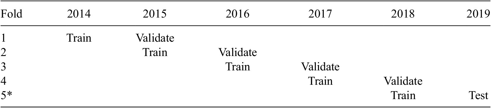
Table 2. Long description
The table consists of seven columns: Fold, 2014, 2015, 2016, 2017, 2018, and 2019.
* Fold 1: 2014 is Train, 2015 is Validate.
* Fold 2: 2015 is Train, 2016 is Validate.
* Fold 3: 2016 is Train, 2017 is Validate.
* Fold 4: 2017 is Train, 2018 is Validate.
* Fold 5 asterisk: 2018 is Train, 2019 is Test.
A note indicates that years 2014 to 2018 for folds 1 to 4 are for train-validate, while year 2019 in fold 5 is for test.
Note: Years 2014–2018, folds 1–4: train-validate. Year 2019, fold
$ {5}^{\ast } $
 : test.
The rationale for the time series CV split is to validate models in a realistic and “causal” scenario, where “causal” refers to the temporal order of train and validate-test sets, not to interventions or counterfactual risk prediction. In this scenario, predictions are only made on the basis of earlier data, as opposed to, say, a traditional 5-fold CV split, in which each of the years 2014–2018 would be set apart as the test set. The moving window split was used, first, because it reveals the tendencies of distribution shift. Second, it is computationally less demanding than the growing window split, in which years up to
$ t-1 $
 are used to train and year
$ t $
are used to train and year
$ t $
 is used to validate.
4. Methods
4.1. Predictive performance metrics
The metric used to assess the predictive performance of ML models is ROC-AUC (Area-Under-Curve of the Receiver Operating Characteristic), AUC for short (Fawcett, Reference Fawcett2006). AUC measures the quality of predicted scores instead of (binary) decisions like predictive accuracy. AUC takes values in
$ \left[0,1\right] $
 , where
$ 0.5 $
, where
$ 0.5 $
 corresponds to a random classifier, and
$ 1 $
corresponds to a random classifier, and
$ 1 $
 to a perfect classifier. The higher the AUC is above
$ 0.5 $
to a perfect classifier. The higher the AUC is above
$ 0.5 $
 , the better is the classifier. Operationally, AUC is the probability that a randomly chosen positive case has a higher predicted score than a randomly chosen negative case. The reason for using AUC instead of predictive accuracy is that AUC has several beneficial properties. First, it is a threshold-independent measure and only depends on a model’s ability to order inputs by risk. Second, it is a better measure of performance under class imbalance, as in the case of the present data, with approximately 20% of cases in the positive class. For specific applications, a threshold can be chosen based on contextual factors, turning the predicted score into a binary risk prediction. If so, accuracy and other functions of the confusion matrix, such as FPR, can be used to assess predictive performance.
Uncertainty in AUC was quantified for the comparison of XGB, a black-box model, and EBM, an interpretable model. First, 500 paired bootstrap resamples were performed separately for each validation year and the test year; stratification was used to preserve the class distribution. Models were trained once per year. The bootstrap was applied to each validation and test dataset. For each resample, AUC was computed for each model. Second, for each resample, the
$ \Delta $
 -AUC (difference between the AUCs of XGB and EBM) was computed. For each year, this yielded 500 bootstrapped
$ \Delta $
-AUC (difference between the AUCs of XGB and EBM) was computed. For each year, this yielded 500 bootstrapped
$ \Delta $
 -AUCs. Third,
$ 95\% $
-AUCs. Third,
$ 95\% $
 percentile bootstrap confidence intervals were computed for each year. Additionally, paired, two-sided Wilcoxon tests were performed for each year of bootstrapped
$ \Delta $
percentile bootstrap confidence intervals were computed for each year. Additionally, paired, two-sided Wilcoxon tests were performed for each year of bootstrapped
$ \Delta $
 -AUCs, testing the null hypothesis that the median difference is
$ 0 $
-AUCs, testing the null hypothesis that the median difference is
$ 0 $
 , yielding 5 p-values for 5 years.
4.2. Black-box models
Three so-called black-box models were tested. All three are considered to be black-box models because, while they are based on decision trees, which are considered to be interpretable (Hastie et al., Reference Hastie, Tibshirani and Friedman2009; Räz, Reference Räz2024a), they use large tree ensembles, which makes them hard to understand. Hyperparameter settings for all models except XGB (and EBM, see later) were taken from Gasser (Reference Gasser2022), who trained the same models on the basis of the same (raw) data. For XGB and EBM, systematic hyperparameter tuning was performed. For the hyperparameters of all models and details, see the Appendix, in particular Table B1.
4.2.1. Random forests (RF)
This is a tree ensemble method, based on bootstrap aggregation (bagging) and developed by Breiman (Reference Breiman2001). RF is relatively simple to train and tune and therefore a popular method (Hastie et al., Reference Hastie, Tibshirani and Friedman2009, p. 587). Several agencies in OECD countries have used RF for statistical profiling (Desiere et al., Reference Desiere, Langenbucher and Struyven2019, Table 1).
4.2.2. Gradient boosting (GB)
This tree method was originally developed by Friedman (Reference Friedman2001). GB is more prone to overfitting than RF. According to Desiere et al. (Reference Desiere, Langenbucher and Struyven2019; Table 1). New Zealand has used GB for statistical profiling.
4.2.3. Extreme gradient boosting (XGB)
This is a modification of GB, developed by Chen and Guestrin (Reference Chen and Guestrin2016), so as to make the method suitable for large datasets. It is much faster than GB and considered to be the state-of-the-art model for tabular data (see Shwartz-Ziv and Armon, Reference Shwartz-Ziv and Armon2022). If the main goal is high predictive performance, XGB may be the best choice among black-box models.
4.3. Interpretable models
Two interpretable models were tested. Both of these models are globally interpretable, meaning that the entire prediction function can be visually inspected and understood (Molnar, Reference Molnar2020; Räz, Reference Räz2024a).
4.3.1. Logistic regression (LR)
This is a linear model for classification tasks (see Hastie et al., Reference Hastie, Tibshirani and Friedman2009). It is interpretable via its coefficients. Its interpretability was enhanced by using the Lasso (Ibid.), also called
$ {L}_1 $
 regularization. By increasing
$ {L}_1 $
regularization. By increasing
$ {L}_1 $
 regularization, one forces more and more coefficients to be zero, making the model smaller and thus more interpretable. Data was preprocessed before training, as required for consistent use of
$ {L}_1 $
regularization, one forces more and more coefficients to be zero, making the model smaller and thus more interpretable. Data was preprocessed before training, as required for consistent use of
$ {L}_1 $
 regularization. LR is the most popular LTU risk model in the OECD, with six countries using it (see survey in Desiere et al., Reference Desiere, Langenbucher and Struyven2019).
4.3.2. Explainable boosting machines (EBM)
This is a generalized additive model (GAM): the prediction function has the form
$ f(X)={f}_1\left({X}_1\right)+\dots +{f}_n\left({X}_n\right)+{f}_{ij}\left({X}_i,{X}_j\right)+\dots +{f}_{kl}\left({X}_k,{X}_l\right) $
 , with
$ i\ne j,k\ne l\in 1,\dots, n $
, with
$ i\ne j,k\ne l\in 1,\dots, n $
 , that is, it is a sum of (nonlinear) functions of individual variables (main effects) and variable pairs (interactions). It was introduced by Lou et al. (Reference Lou, Caruana, Gehrke and Hooker2013); the implementation by Nori et al. (Reference Nori, Jenkins, Koch and Caruana2019) was used. (EBM is a relatively recent model based on GAM. GAM was invented in the 1980s, see (Hastie and Tibshirani, Reference Hastie and Tibshirani1990), and is an active area of research. It would be worthwhile to explore other variants, such as classical GAM with smoothing splines (Ibid.), sparse GAM (Ravikumar et al., Reference Ravikumar, Lafferty, Liu and Wasserman2009), or more recent GAMs based on neural networks (Agarwal et al., Reference Agarwal, Melnick, Frosst, Zhang, Lengerich, Caruana and Hinton2021).) Internally, EBM employs gradient boosting to learn individual feature functions. As a GAM, it is globally interpretable: the component functions of the form
$ {f}_m\left({X}_m\right) $
, that is, it is a sum of (nonlinear) functions of individual variables (main effects) and variable pairs (interactions). It was introduced by Lou et al. (Reference Lou, Caruana, Gehrke and Hooker2013); the implementation by Nori et al. (Reference Nori, Jenkins, Koch and Caruana2019) was used. (EBM is a relatively recent model based on GAM. GAM was invented in the 1980s, see (Hastie and Tibshirani, Reference Hastie and Tibshirani1990), and is an active area of research. It would be worthwhile to explore other variants, such as classical GAM with smoothing splines (Ibid.), sparse GAM (Ravikumar et al., Reference Ravikumar, Lafferty, Liu and Wasserman2009), or more recent GAMs based on neural networks (Agarwal et al., Reference Agarwal, Melnick, Frosst, Zhang, Lengerich, Caruana and Hinton2021).) Internally, EBM employs gradient boosting to learn individual feature functions. As a GAM, it is globally interpretable: the component functions of the form
$ {f}_m\left({X}_m\right) $
 and
$ {f}_{ij}\left({X}_i,{X}_j\right) $
and
$ {f}_{ij}\left({X}_i,{X}_j\right) $
 are nonlinear, but limited to pairwise interactions. They can therefore be individually inspected, visually understood, and modified. As explained subsequently, some of the component functions in the present paper were edited after inspection to reflect domain knowledge (see Figure 4). Inspection and editing of component functions are only possible because EBM is additive and limited to interactions of degree two. This would be much harder, if not impossible, for black-box models like XGB. Local explanations, which provide insight into how individual predictions are made, can be constructed in the form of feature importance plots. A (fictitious) example of a local explanation is given in the Appendix (Figure C7). Local explanations show how much the values of
$ f $
are nonlinear, but limited to pairwise interactions. They can therefore be individually inspected, visually understood, and modified. As explained subsequently, some of the component functions in the present paper were edited after inspection to reflect domain knowledge (see Figure 4). Inspection and editing of component functions are only possible because EBM is additive and limited to interactions of degree two. This would be much harder, if not impossible, for black-box models like XGB. Local explanations, which provide insight into how individual predictions are made, can be constructed in the form of feature importance plots. A (fictitious) example of a local explanation is given in the Appendix (Figure C7). Local explanations show how much the values of
$ f $
 for an individual’s features contribute positively or negatively to that individual’s total score. Local explanations of EBM predictions are faithful to the model: They are directly derived from the actual predictor function
$ f $
for an individual’s features contribute positively or negatively to that individual’s total score. Local explanations of EBM predictions are faithful to the model: They are directly derived from the actual predictor function
$ f $
 and do not rely on approximations or surrogate models. In sum, EBM provides global interpretability, in contrast to, for instance, post-hoc explanations provided by SHAP applied to RF.
4.4. Interpretability enhancement for EBM and LR
In addition to the off-the-shelf version of EBM (and LR), additional steps were taken to improve two dimensions of interpretability. The subsequently given description is more detailed because these methods are not part of the EBM implementation.
4.4.1. Sparsity
The interpretability of both LR and EBM may benefit from sparsity, that is, from only using a subset of variables. There are different methods to achieve sparsity in linear (and additive) models. First, the Lasso, or
$ {L}_1 $
 regularization, enforces features to become zero “all at once.” In the present paper, the Lasso was tested for both LR and EBM. For LR, it worked as intended (see Figure C1, Appendix); for EBM, the Lasso did not yield satisfactory sparsity while preserving predictive performance. Therefore, backward selection (Hastie et al., Reference Hastie, Tibshirani and Friedman2009, Section 3.3) was used to create sparse EBMs (see Figure C2, Appendix). In a first experiment, a full EBM with 57 main features, fit to the first training fold (year 2014), was taken as a starting point. The least important features (average feature importance) of this EBM were removed in steps of five, yielding a sequence of
$ \left(55,50,45,\dots, 5\right) $
regularization, enforces features to become zero “all at once.” In the present paper, the Lasso was tested for both LR and EBM. For LR, it worked as intended (see Figure C1, Appendix); for EBM, the Lasso did not yield satisfactory sparsity while preserving predictive performance. Therefore, backward selection (Hastie et al., Reference Hastie, Tibshirani and Friedman2009, Section 3.3) was used to create sparse EBMs (see Figure C2, Appendix). In a first experiment, a full EBM with 57 main features, fit to the first training fold (year 2014), was taken as a starting point. The least important features (average feature importance) of this EBM were removed in steps of five, yielding a sequence of
$ \left(55,50,45,\dots, 5\right) $
 features (see Figure C3, Appendix for average feature importance). New EBMs were fit to these subsets, and the predictive performance was assessed. In a second experiment, three models of sparsities 45, 30, and 15 were fit to the four train-validate folds (years 2014-18), based on the 45, 30, 15 most important main features of the full EBM trained on that fold. Backward selection is a relatively rough method, but it is computationally tractable and yields a first indication of the extent to which sparsity in EBM can be achieved without large performance losses.
4.4.2. Smoothing numerical features
EBM in the off-the-shelf version offers in-principle interpretability of individual feature functions by visual inspection. However, there is no guarantee that these functions are “simple.” The predictor functions of five numerical features show large local fluctuations and quasi-discontinuities (see Figure 4 for an example). These fluctuations were classified as artifacts by a domain expert and may be due to overfitting. Large local fluctuations are problematic for at least two reasons. First, they prevent global interpretability in that they make it hard to grasp the behavior of feature functions. Second, they are problematic in view of individual predictions and their explanation. If a jobseeker is located at a point of a feature function with a large deviation from the local trend, and this deviation is due to overfitting, it is hard to justify the corresponding risk prediction as fair. (This issue is closely related to the notion of individual fairness, according to which people with similar properties should be treated similarly (Dwork et al., Reference Dwork, Hardt, Pitassi, Reingold and Zemel2012). Thus, this is an instance where considerations of interpretability and fairness interact.)
After testing several methods that remove artifacts in feature functions, it was decided to use smoothing cubic splines (Hastie et al., Reference Hastie, Tibshirani and Friedman2009, Section 2.8.1.) Smoothing splines are a statistical method to construct a smooth version of a “rough” function. In a first step, smoothing was applied to individual, off-the-shelf numerical feature functions of one sparse EBM-30 in the first fold. The EBM-30 was chosen to get an idea of how smoothing and sparsity interact. Different smoothing parameters for different features were chosen based on a trade-off between the degree of smoothing and overall performance (AUC). In a second step, the goal was to understand how smoothing affects performance. To do so, the same degree of smoothing was applied uniformly to four sparse EBM from the four train-validate folds. Then the predictive performance in the four folds was measured. (Note that historically, GAMs were trained using smoothing splines, see (Hastie and Tibshirani, Reference Hastie and Tibshirani1990). A second method, GAMChanger, introduced by Wang et al. (Reference Wang, Kale, Nori, Stella, Nunnally, Chau, Vorvoreanu, Vaughan and Caruana2021), was also tested. GAMChanger allows users to manually edit single feature functions in a graphical user interface and to check how edits affect performance metrics on a data sample. Unfortunately, the functionality of GAMChanger was limited in practice—storing results did not work as intended.)
4.5. Fairness
There have been many proposals to mitigate group disparities or unfairness in the context of ML. Technically, there are three types of fairness mitigation: Preprocessing (changing inputs), in-processing (changing the training process, for example, using regularization), and postprocessing (changing outputs of a trained model; see Barocas et al., Reference Barocas, Hardt and Narayanan2022). In the present paper, a postprocessing method (Hardt et al., Reference Hardt, Price and Srebro2016) will be used to equalize false positives across groups. False positives were previously investigated as an important fairness metric in the context of LTU profiling by Desiere and Struyven (Reference Desiere and Struyven2021). Here, a full EBM from the first fold was taken as a base model. Postprocessing only affects the choice of decision thresholds and does not depend on the internal structure of the model. Therefore, the interpretability of models is preserved under postprocessing.
Two sets of experiments were performed. In the first set of experiments, fairness was investigated with respect to three age groups (15–29, 30–44, 45–65) to show the feasibility of the current approach. In a second set of experiments, fairness was investigated with respect to the full intersection of three attributes: age, gender, and residency status (a proxy for nationality and ethnicity). For age, the same groups as in the first experiments were used. For gender, the binary attribute (male, female) available in the data was used. For residency status, permanent vs. nonpermanent residency was used. (These choices are debatable and should be seen as a first approximation to intersectional fairness. For gender, nonbinary attributes could be used, but are currently not contained in the data. Permanent residency encompasses Swiss citizens and foreigners who have been in Switzerland for five or ten years; it is more easily obtainable for citizens of some EU countries. Instead of residency status, information about specific ethnicities could be used, because discrimination affects some ethnicities more (see Section 2.3). However, direct information about ethnicity is currently not contained in the data.) The intersection of these three attributes, 3 age groups x 2 genders x 2 residency status groups, yields 12 groups in total. It can be challenging to measure fairness in a statistically reliable way if some group intersections become small (Morina et al., Reference Morina, Oliinyk, Waton, Marusic and Georgatzis2019). Group sizes were examined to guarantee a stable estimation of FP (see Agresti, Reference Agresti2013). The experiments take the following steps:
-
1. A threshold is chosen, which yields binary risk predictions. The choice of threshold depends on the purpose for which the prediction is used. Here, the threshold is chosen such that 80% of all true positives are identified. This corresponds to a true positive rate (TPR), or recall, of $ 0.8 $
 . This choice can be motivated by a requirement to make targeting efficient (see Gasser, Reference Gasser2022). The fairness of the resulting (binary) predictor with respect to protected attributes (age and group intersections) is then examined. Specifically, the confusion matrix of all groups of the resulting predictor is examined. (The confusion matrix tabulates four statistics of binary predictors: true positives, false positives, true negatives, false negatives. The confusion matrix is normalized by the total count (TP + FP + TN + FN) to make results comparable across groups.)
 -
2. The postprocessing method of Hardt et al. (Reference Hardt, Price and Srebro2016) is used to equalize FPRs for all groups under an accuracy constraint. The implementation of Weerts et al. (Reference Weerts, Dudík, Edgar, Jalali, Lutz and Madaio2023) was employed. The postprocessing finds separate thresholds for the protected attributes such that FPRs are equalized. In order to preserve the original goal of a given TPR to some extent, balanced accuracy is used as a constraint. Balanced accuracy is defined as (TPR + TNR)/2; note that TNR = 1 − FPR. It is then determined how postprocessing affects the confusion matrix and performance metrics like accuracy.

4.6. Use of AI tools
AI assistants (ChatGPT.com in the free version, and Claude.ai in the free version and the Pro version) have been used during 2025 to generate code for this project, including feature engineering, statistical analysis, and code to create figures (not figures themselves). All code has been reviewed and approved by the author, and the author is solely responsible for the correctness of the code.
5. Results
5.1. Predictive performance
The results of the predictive performance (AUC) of the five models tested can be seen in Figure 1 (for numbers see Table C1, Appendix). Two black-box models (GB, XGB) show the best overall predictive performance, with the exception of the drop of GB in the test year. XGB shows the best overall performance for all validate and test years. The relatively low performance of RF is more surprising. Turning to the interpretable models, LR shows the overall worst relative performance of all models in validation, but improves in the test year, surpassing RF and GB. Finally, EBM results are consistent with claims in the literature that EBM performs similar to the best black-box models. EBM performs worse than the best black-box model, but the performance difference is relatively minor. The comparatively high performance of EBM is one of the main results of this paper: Interpretable models show good predictive performance in a realistic scenario while being transparent. The performance obtained here is in a similar range as in other recent empirical studies, roughly in an AUC range of 0.7–0.8 (Desiere et al., Reference Desiere, Langenbucher and Struyven2019; Dossche et al., Reference Dossche, Vansteenkiste, Baesens and Lemahieu2024). Note that the results obtained by Gasser (Reference Gasser2022) on the same data show a qualitative agreement in performance with results obtained here, but AUC found by Gasser was slightly higher. (Note also that while the computational cost of model fitting was not evaluated systematically, XGB was found to be fast, taking few minutes to fit four models to four folds. EBM was found to be the slowest model, taking approximately 20 minutes to fit four models to four folds. All experiments were performed on a standard desktop computer.)
Performance Score (AUC) for five folds. Years 2015–2018: validate; year 2019: test.
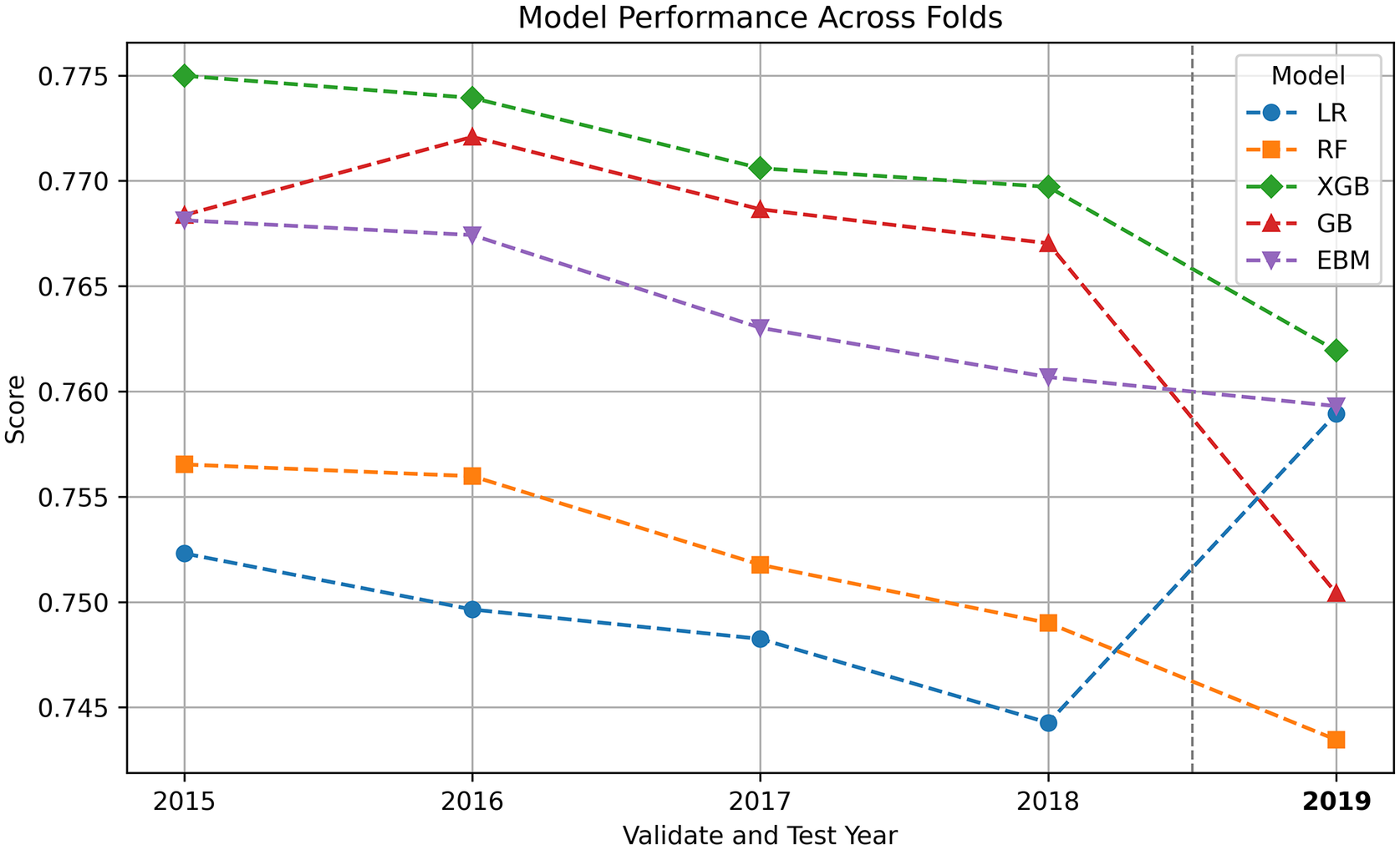
Figure 1. Long description
The x-axis is labeled Validate and Test Year with markers for 2015, 2016, 2017, 2018, and 2019. The y-axis is labeled Score and ranges from 0.745 to 0.775. A vertical dashed line between 2018 and 2019 separates the validation period from the test year. Five models are represented by dashed lines with unique markers.
* X G B (green diamonds) starts highest at 0.775 in 2015, gradually declining to 0.770 in 2018, then dropping to 0.762 in 2019.
* G B (red triangles) starts at 0.768, peaks at 0.772 in 2016, then declines sharply to 0.750 in 2019.
* E B M (purple inverted triangles) starts at 0.768 and shows a steady, slight downward trend to 0.759 by 2019.
* R F (orange squares) starts at 0.757 and shows a consistent linear decrease to 0.744 in 2019.
* L R (blue circles) starts at 0.752, decreases to a low of 0.744 in 2018, but then shows a sharp increase to 0.759 in 2019, converging with the E B M model.
The temporal evolution of predictive performances is noteworthy. The moving window time series split keeps conditions (size and temporal relation of train and validate sets) constant, which suggests that the drop in predictive performance over time is due to a shift in the data distribution. More experiments are necessary to better understand this phenomenon, for instance, to examine the effect of also including less recent data in training. The origin of the qualitative shift in the test year (drop of GB, rise of LR) is unknown; care was taken to use identical data pipelines for validation and testing. The drop of GB could be due to overfitting in validation; the reason for the rise of LR is unknown. The changes in “deployment-like” conditions (test year) show the importance of continuous monitoring and retraining of operational systems.
The difference in predictive performance between XGB and EBM was further investigated with respect to its uncertainty (see Figure 2). Across all validation and test years, there is a small (between
$ 0.002 $
 and
$ 0.009 $
and
$ 0.009 $
 ) but consistent difference between the AUC of XGB and EBM, with XGB performing better. The
$ 95\% $
) but consistent difference between the AUC of XGB and EBM, with XGB performing better. The
$ 95\% $
 confidence intervals exclude zero. The differences are statistically significant (different from zero) for all five years according to paired, two-sided Wilcoxon tests, with
$ p<0.001 $
confidence intervals exclude zero. The differences are statistically significant (different from zero) for all five years according to paired, two-sided Wilcoxon tests, with
$ p<0.001 $
 .
.
Uncertainty quantification for five folds; average AUC difference and 95% confidence intervals of XGB and EBM. Years 2015–2018: validate; year 2019: test.
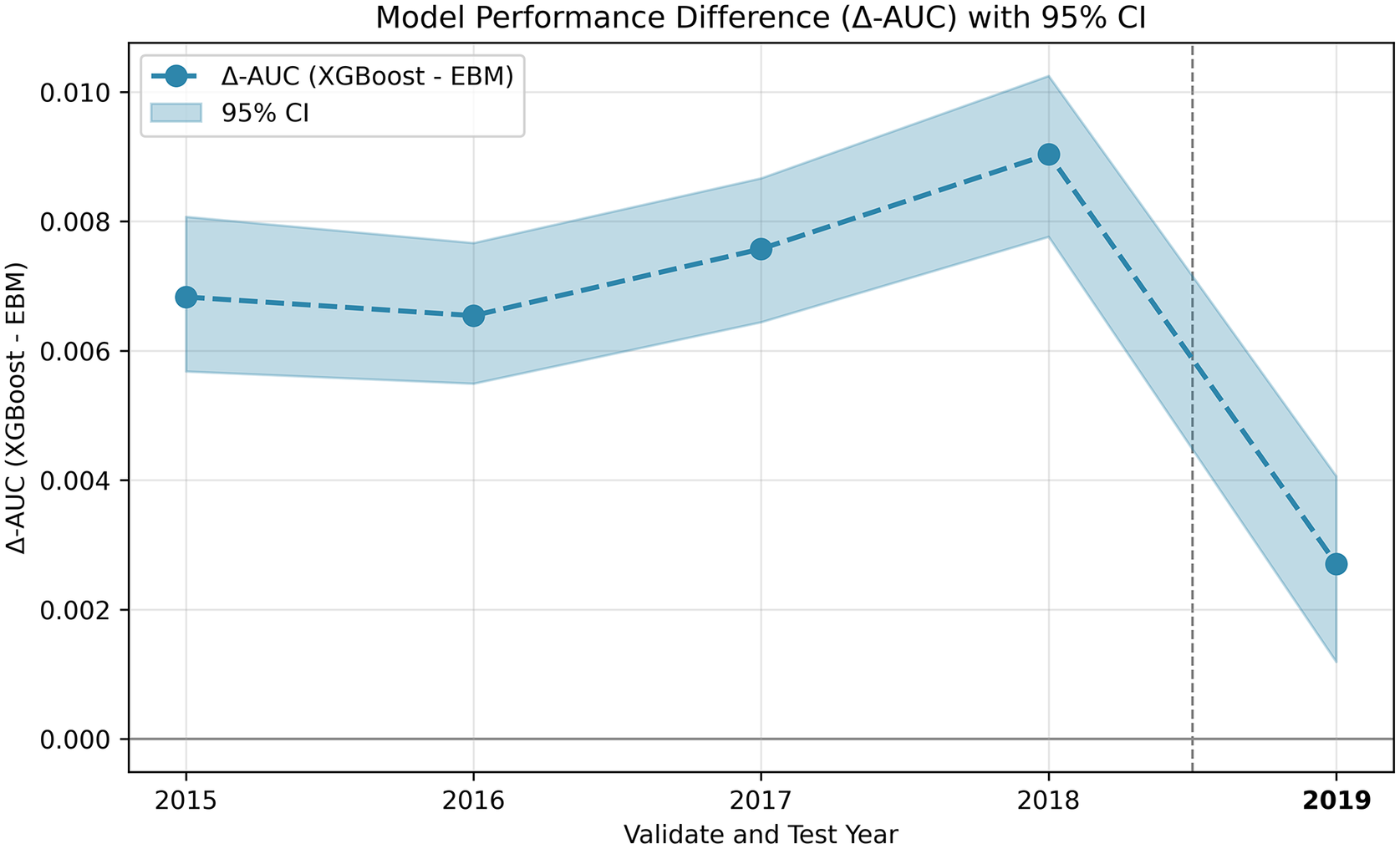
Figure 2. Long description
The horizontal X axis is labeled Validate and Test Year with markers for 2015, 2016, 2017, 2018, and 2019. The vertical Y axis is labeled Delta A U C open parenthesis X G B o o s t minus E B M close parenthesis with values ranging from 0.000 to 0.010. A dashed line with circular markers represents the mean difference.
* In 2015, the Delta A U C is approximately 0.007.
* In 2016, it slightly dips to 0.0065.
* In 2017, it rises to approximately 0.0075.
* In 2018, it peaks at 0.009.
* A vertical dashed line separates 2018 from 2019, indicating the transition from validation to test data.
* In 2019, the value drops sharply to approximately 0.0025.
A light blue shaded region surrounds the line, representing the 95 percent confidence interval. This interval remains relatively consistent in width until 2018, where it reaches its highest point, before narrowing as it descends toward the 2019 test year marker. All data points remain above the 0.000 baseline.
5.2. Interpretability: sparsity
For LR, sparsity induced by
$ {L}_1 $
 regularization shows that using a parameter setting of
$ 0.1 $
regularization shows that using a parameter setting of
$ 0.1 $
 leads to no appreciable drop in AUC with a small increase in sparsity:
$ 115 $
leads to no appreciable drop in AUC with a small increase in sparsity:
$ 115 $
 of
$ 120 $
of
$ 120 $
 features are nonzero (see Figure C1). A setting of
$ 0.01 $
features are nonzero (see Figure C1). A setting of
$ 0.01 $
 leads to a small drop in AUC while
$ 79 $
leads to a small drop in AUC while
$ 79 $
 of
$ 120 $
of
$ 120 $
 features are nonzero. The first setting, as the more conservative choice, was used in the overall performance evaluation. Dropping a third of all features may lead to a small drop in AUC for LR, which may be worth considering in terms of interpretability.
For EBM, the first experiment with backward selection (see Figure C2), in which main features were dropped in steps of
$ 5 $
 , shows that dropping up to a third of main features yields only small drops in AUC, and that a model with as little as
$ 5 $
, shows that dropping up to a third of main features yields only small drops in AUC, and that a model with as little as
$ 5 $
 main features has an AUC of just below
$ 0.74 $
main features has an AUC of just below
$ 0.74 $
 , which shows that the bulk of predictive performance is due to relatively few main features. Note that the size of models drops linearly, because for each sparsity level
$ n $
, which shows that the bulk of predictive performance is due to relatively few main features. Note that the size of models drops linearly, because for each sparsity level
$ n $
 ,
$ 0.5\cdot n $
,
$ 0.5\cdot n $
 interaction terms were included. In the second experiment, the findings of the first experiment for EBM were confirmed to be robust across all validation folds, with backward selection dropping
$ 15 $
interaction terms were included. In the second experiment, the findings of the first experiment for EBM were confirmed to be robust across all validation folds, with backward selection dropping
$ 15 $
 main features at a time (see Figure 3). The results show that using
$ 45 $
main features at a time (see Figure 3). The results show that using
$ 45 $
 main features only yields a relatively small drop in AUC, while the drop in performance is larger for the two sparser models. EBM-15 shows higher AUC than LR on the validation fold; this result may not hold for the test fold. Overall, these results confirm the well-known accuracy–interpretability trade-off: The smaller and thus simpler the model, the less performant it is. They also confirm that a sizable portion of features can be dropped without large losses in predictive performance.
Performance Score (AUC) for XGB, full EBM, LR, as well as three sparse EBMs with 45, 30, 15 most important main features. Results for LR, XGB, and EBM are the same as in Figure 1 and included for reference.
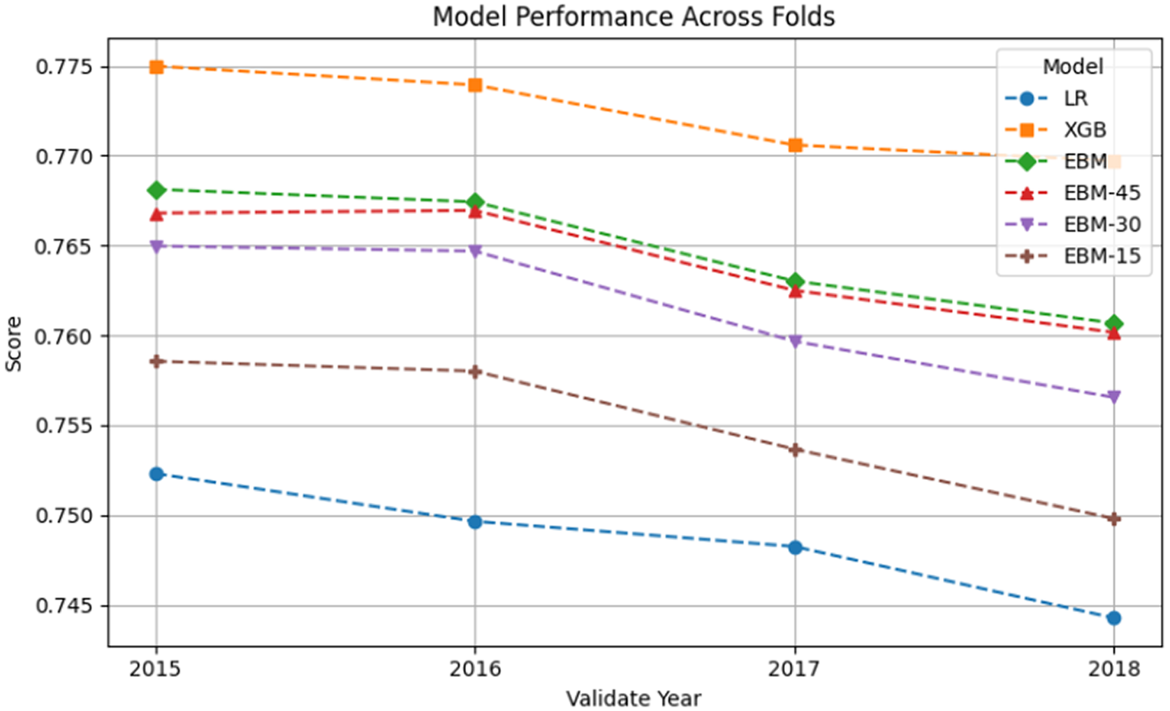
Figure 3. Long description
The x-axis is labeled Validate Year with four discrete points: 2015, 2016, 2017, and 2018. The y-axis is labeled Score and ranges from 0.745 to 0.775. Six dashed lines represent different models.
* X G B (orange squares) maintains the highest performance, starting at 0.775 in 2015 and gradually declining to approximately 0.770 by 2018.
* E B M (green diamonds) and E B M dash 45 (red triangles) follow a nearly identical path just below X G B, starting around 0.768 and ending near 0.760.
* E B M dash 30 (purple inverted triangles) starts at 0.765 and declines to approximately 0.757.
* E B M dash 15 (brown plus signs) starts at 0.758 and declines to 0.750.
* L R (blue circles) shows the lowest performance, starting at 0.752 and ending at approximately 0.744.
All models exhibit a consistent downward trend in performance score as the validation year progresses from 2015 to 2018.
5.3. Interpretability: smoothing numerical features
The need for smoothing numerical feature functions can be motivated by looking at an example of a raw feature (sparse EBM-30), together with the smoothed version, shown in Figure 4 (see Figures C4, C5, C6 in the Appendix for other smoothed features). If one examines the raw main feature of insured income, the overall trend of the plot is relatively easy to grasp, but local fluctuations are hard to understand and justify. Local fluctuations, like the large drop and spike to the very left, are likely artifacts and due to overfitting. The smoothing spline retains the overall trend of the raw function while removing artifacts. For example, the smoothing retains a clear nonlinearity, with a rise in LTU risk for incomes below 4k, a dropping risk for incomes between roughly 4k and 6k, and a rise for incomes above 6k.
Numerical feature “insured income” (vers_verdienst), in raw version (off-the-shelf EBM) and after applying smoothing spline with smoothing parameter
$ \lambda $
 ; insured income in CHF. The score is the contribution of the feature to the risk of LTU.
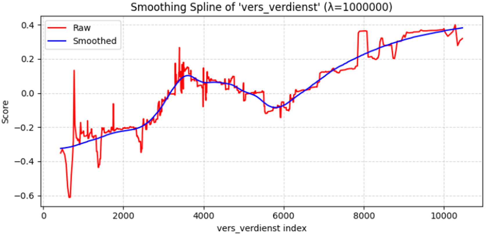
Figure 4. Long description
The graph is titled Smoothing Spline of vers underscore verdienst with lambda equal to 1000000. The horizontal X axis is labeled vers underscore verdienst index, ranging from 0 to 10000. The vertical Y axis is labeled Score, ranging from negative 0.6 to 0.4.
Two data series are plotted:
* A red line labeled Raw shows highly volatile, jagged fluctuations with sharp peaks and deep troughs. It begins with a sharp drop to negative 0.6 near the 500 index mark, followed by erratic spikes and plateaus as it trends generally upward.
* A blue line labeled Smoothed represents an E B M model. It follows the general trend of the red line but eliminates the noise, showing a gradual S-shaped curve. It starts at negative 0.3, rises to a local peak of 0.1 at the 3500 index, dips slightly to 0.0 at the 5500 index, and then rises steadily to nearly 0.4 at the 10000 index mark.
The background features a light gray dashed grid.
Figure 5 shows the results of applying uniform smoothing to four sparse EBM-30 in the four train-validate folds with respect to performance. In each of the four folds, smoothing was applied to the following features: insured income, age, rate of desired employment, # months of previous contributions (see Figure 4 and Appendix). A further feature, rate of previous employment, was also smoothed, but not further investigated because it was not in the top 30 main features in all four folds. There is a relatively modest overall drop in predictive performance from EBM-30 to the smoothed version EBM-30-SM. This is, again, a manifestation of the accuracy–interpretability trade-off. The drop is more appreciable in the
$ 2016 $
 fold, which shows that some performance risk is incurred by smoothing. It should be stressed that there is a lot of opportunity for tuning the smoothing parameter based on various considerations. For example, smoothing can be used more aggressively for features with lower average importance, and more conservatively for features with higher importance. A more systematic exploration of the accuracy–interpretability trade-off could be performed by plotting the AUC against a parameter range; note that the shape of the resulting feature function needs to be inspected separately. The uniform use of the same parameter choice for the different validation sets (years) indicates that the empirical risk (AUC loss) of this parameter choice is low.
Performance Score (AUC) for original EBM-30 (sparse EBM with 30 most important main features), and smoothed version EBM-30-SM (EBM-30 with smoothed numerical features). XGB, full EBM, LR for reference.
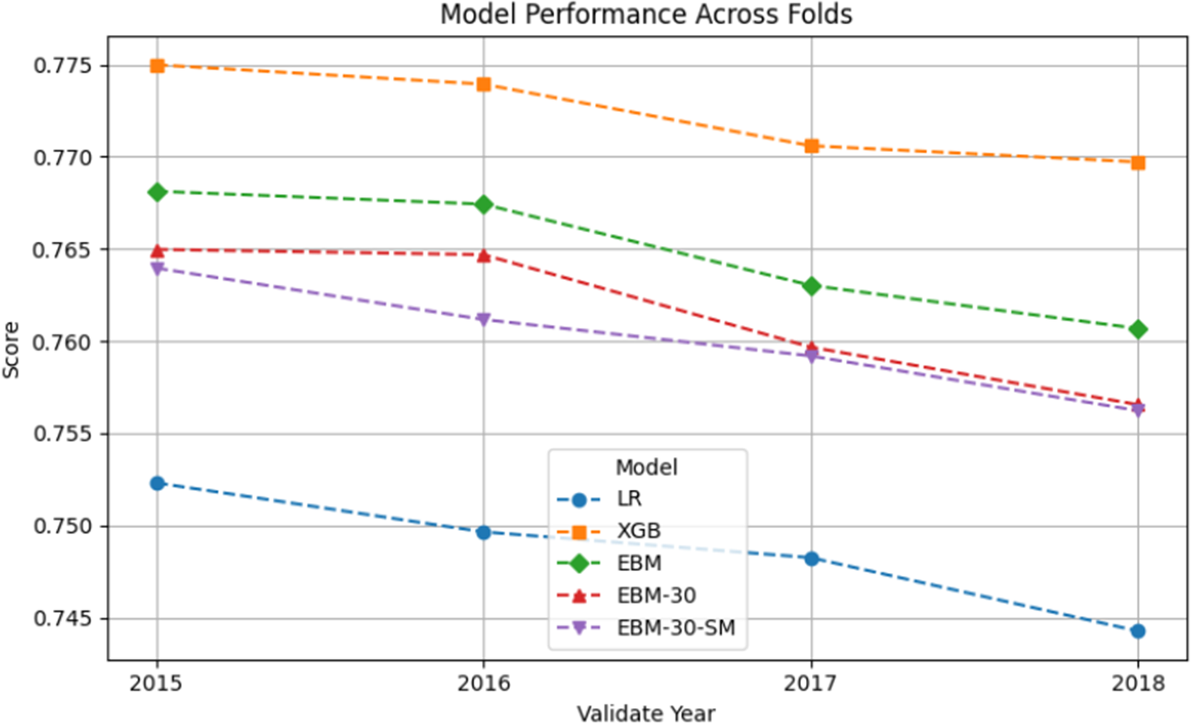
Figure 5. Long description
The horizontal X axis is labeled Validate Year and includes four discrete points: 2015, 2016, 2017, and 2018. The vertical Y axis is labeled Score and ranges from 0.745 to 0.775 in increments of 0.005. Five dashed lines with markers represent different models.
* X G B (orange squares) starts at the highest score of 0.775 in 2015 and declines steadily to approximately 0.770 by 2018.
* E B M (green diamonds) starts at 0.768 and follows a similar downward slope, ending at approximately 0.761.
* E B M dash 30 (red triangles) starts at 0.765 and declines to approximately 0.757.
* E B M dash 30 dash S M (purple inverted triangles) starts at 0.764, slightly below E B M dash 30, and converges with it at the 0.757 mark by 2018.
* L R (blue circles) maintains the lowest performance throughout, starting at 0.752 and dropping to approximately 0.744.
All models exhibit a nearly parallel downward trend over the four-year period.
5.4. Fairness
The results of fairness mitigation with respect to three age groups is described first. Figure 6 shows the results of choosing the threshold at which 80% of all true positives are identified (TPR, see performance metrics), making the prediction binary. It can be observed that (normalized) false positives (FP) vary quite strongly between the three age groups: normalized false positives go up with age. This is to be expected, as the LTU risk also rises with age. Note that the accuracy is moderate at 63%, but that accuracy is not the objective; the threshold was chosen for the given TPR.
Confusion matrices (normalized) for three age groups, and overall performance metrics, before fairness mitigation.
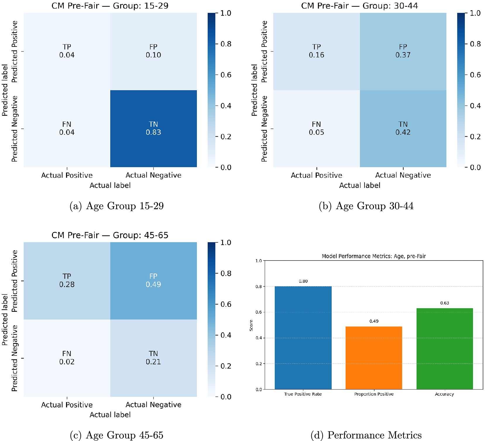
Figure 6. Long description
The figure contains four panels labeled a through d.
Panels a, b, and c are C M Pre-Fair confusion matrices. Each has a Y-axis for Predicted label (Predicted Positive, Predicted Negative) and an X-axis for Actual label (Actual Positive, Actual Negative). A color scale from 0.0 to 1.0 indicates density.
Panel a, Age Group 15 to 29:
* T P (Top-Left): 0.04
* F P (Top-Right): 0.10
* F N (Bottom-Left): 0.04
* T N (Bottom-Right): 0.83. This group shows high True Negative concentration.
Panel b, Age Group 30 to 44:
* T P: 0.16
* F P: 0.37
* F N: 0.05
* T N: 0.42
Panel c, Age Group 45 to 65:
* T P: 0.28
* F P: 0.49
* F N: 0.02
* T N: 0.21. This group shows the highest False Positive rate.
Panel d is a bar chart titled Model Performance Metrics: Age, pre-Fair. The Y-axis is Score from 0.0 to 1.0. Three bars are shown from left to right:
* True Positive Rate: 0.80 (blue bar)
* Proportion Positive: 0.49 (orange bar)
* Accuracy: 0.63 (green bar)
Figure 7 shows the results after applying fairness mitigation, in which separate thresholds are found by group, satisfying FPR under a constraint of balanced accuracy. We observe that normalized false positives (FPs) have become much more equal; in fact, FP is now a bit higher for the “young” age group. The three normalized confusion matrices look more balanced overall, as can be seen by comparing the color codings. Note that normalized false positives were not directly targeted as the fairness objective; rather, the target was FPR and balanced accuracy. Importantly, the original target of 80% TPR is no longer satisfied; TPR is now at 66%. This means that the “fair” predictor, capturing only 2/3 of all positive cases, is not as efficient as the original predictor. The overall accuracy is higher after fairness mitigation.
Confusion matrices (normalized) for three age groups, and overall performance metrics, after fairness mitigation.
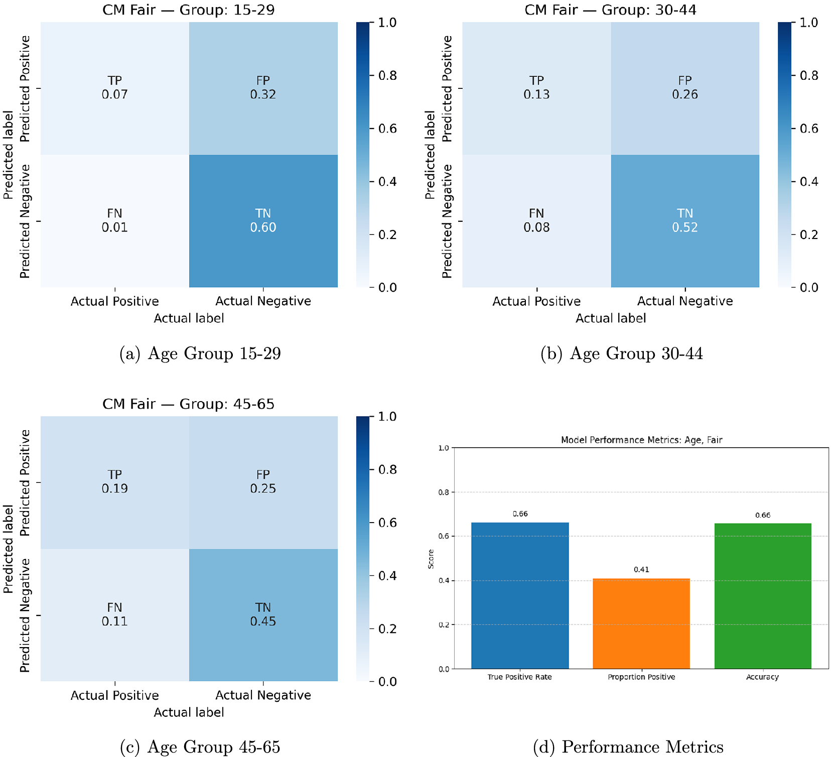
Figure 7. Long description
The figure consists of four panels labeled a through d.
Panels a, b, and c are normalized confusion matrices titled C M Fair for age groups 15 to 29, 30 to 44, and 45 to 65 respectively. Each matrix has Actual Positive and Actual Negative on the x-axis and Predicted Positive and Predicted Negative on the y-axis. A color scale to the right of each matrix ranges from 0.0 in white to 1.0 in dark blue.
* Panel a, Age Group 15 to 29: T P is 0.07, F P is 0.32, F N is 0.01, and T N is 0.60.
* Panel b, Age Group 30 to 44: T P is 0.13, F P is 0.26, F N is 0.08, and T N is 0.52.
* Panel c, Age Group 45 to 65: T P is 0.19, F P is 0.25, F N is 0.11, and T N is 0.45.
Panel d is a bar chart titled Model Performance Metrics Age, Fair. The y-axis is labeled Score from 0.0 to 1.0. The x-axis contains three categories:
* True Positive Rate: A blue bar with a value of 0.66.
* Proportion Positive: An orange bar with a value of 0.41.
* Accuracy: A green bar with a value of 0.66.
The second set of experiments examined 12 group intersections, with three age groups, two genders, and permanent vs. nonpermanent residents. Here, a summary of results is provided (full results can be found in the Appendix, see Figures C9–C11). The size of intersections was checked. All intersections contain more than 2000 cases and more than 400 positive incidences of LTU, which allows a stable estimation of FP. Before fairness mitigation, normalized true positives vary more strongly between the 12 groups than between age groups. The group (age 15–29, male, permanent residents) has the minimum FP of
$ 0.06 $
 ; the group (age 45–65, female, permanent residents) has the maximum FP of
$ 0.55 $
; the group (age 45–65, female, permanent residents) has the maximum FP of
$ 0.55 $
 . However, the trend of lower FP for younger jobseekers from the first set of experiments is preserved.
After fairness mitigation, normalized false positives are much closer together, with minimum FP of
$ 0.22 $
 for group (age 45–65, male, permanent residents), and maximum FP of
$ 0.30 $
for group (age 45–65, male, permanent residents), and maximum FP of
$ 0.30 $
 for group (age 15–29, male and female, permanent residents). The drop of the difference between min and max, from
$ 0.49 $
for group (age 15–29, male and female, permanent residents). The drop of the difference between min and max, from
$ 0.49 $
 before fairness mitigation to
$ 0.08 $
before fairness mitigation to
$ 0.08 $
 after fairness mitigation, is a six-fold reduction of the difference between the best-off and the worst-off group with respect to FP. However, the trend that younger jobseekers have lower false positives is reversed after fairness mitigation—the same reversal can be observed in the first set of experiments. This kind of fairness trade-off is to be expected, and the mitigation performed here should be seen as a first step of a fairness deliberation. Finally, the true positive rate drops more (from
$ 0.8 $
after fairness mitigation, is a six-fold reduction of the difference between the best-off and the worst-off group with respect to FP. However, the trend that younger jobseekers have lower false positives is reversed after fairness mitigation—the same reversal can be observed in the first set of experiments. This kind of fairness trade-off is to be expected, and the mitigation performed here should be seen as a first step of a fairness deliberation. Finally, the true positive rate drops more (from
$ 0.8 $
 to
$ 0.63 $
to
$ 0.63 $
 ) due to mitigation for intersections than for age alone; at the same time, accuracy improves marginally more (from
$ 0.63 $
) due to mitigation for intersections than for age alone; at the same time, accuracy improves marginally more (from
$ 0.63 $
 to
$ 0.67 $
to
$ 0.67 $
 ).
).
6. Discussion
6.1. Contextualization and stakeholder perspective
Let us put the above results in the context of current statistical profiling practices and discuss the ramifications for stakeholders as well as policy lessons of each evaluative dimension.
Predictive performance is one of the most important evaluative dimensions of statistical profiling; it is of high interest to all stakeholder groups. If one takes the predictive performance of the five models evaluated here as an indicator of general predictive performance, then many agencies in the OECD (see Section 2) use suboptimal models: Most agencies that rely on black-box models use RF; the present study found that XGB, the state-of-the-art black-box model, outperforms RF in the present context. Turning to interpretable models, most agencies employ a linear model (LR), which is outperformed by EBM in the present study. EBM is not currently employed in LTU profiling. Notably, the findings reported here contradict claims (e.g., Dossche et al., Reference Dossche, Vansteenkiste, Baesens and Lemahieu2024) that black-box models like RF and XGB outperform inherently interpretable models. Rather, the inherently interpretable EBM outperforms RF and comes close in performance to the best black-box model, with a small AUC gap between XGB and EBM that is statistically significant. All results obtained here are valid for the present data and do not necessarily generalize to other contexts.
These findings do not directly translate into policy recommendations. For one, as stressed earlier, predictive performance is only one evaluative dimension. For example, agencies currently employing RF or another black-box model need not necessarily switch to XGB, but could evaluate EBM as an interpretable alternative, which may be superior to RF in terms of predictive performance. What is more, agencies employing LR already have an interpretable model in place, and the cost of disrupting a working and accepted system may be relatively high, because the switch from LR to the predictively superior EBM may pose challenges of interpretation. The same is true for agencies with an operational black-box model.
Interpretability is an important desideratum of statistical profiling for stakeholders. Different stakeholder groups are interested in different aspects of interpretability offered by EBM and LR. Interpretability is a property of algorithms that has been argued to decrease algorithm aversion, the discounting of algorithmic decisions that affect one’s own or others’ decisions (Mahmud et al., Reference Mahmud, Islam, Ahmed and Smolander2022). This concerns all stakeholders, but jobseekers and caseworkers in particular:
Jobseekers profit from insight into why they have a certain risk prediction. For example, they can inspect the feature function “insured income” (Figure 4) and read off how their income impacts their LTU risk. Both LR and EBM offer the possibility of providing local explanations of single predictions, with the key property that local explanations are faithful to the model, not approximations like explanations of black-box models. On the basis of such explanations (see Figure C7 for a fictitious example), jobseekers get the opportunity to adapt their future behavior, but also to contest predictions (Karimi et al., Reference Karimi, Barthe, Schölkopf and Valera2022). Of course, risk predictions can still be incorrect: EBM offers higher predictive performance than LR, but is nevertheless an imperfect, statistical instrument.
Caseworkers profit from the possibility of offering reasons for risk predictions to their clients, for example on the basis of a local explanation, and to develop personalized mitigation strategies on this basis. (To offer a fictitious example: A caseworker may recommend to lower income expectations to jobseekers with incomes above 6k, which may lower their risk (assuming that insured income is closely related to income expectations); however, if a client has an insured income between 4k and 6k, this may not be advisable.) Interpretable models may offer a path to a more participatory use of statistical profiling, which may encourage use of profiling tools and lower resistance to statistical profiling, a kind of algorithm aversion that has been observed in Switzerland (Arni and Schiprowski, Reference Arni and Schiprowski2016). Both LR and EBM offer a range of different sparsities (Section 5.2). Sparse, smaller models can lower workload and cognitive load of caseworkers. Insight into the risk distributions for single features provided by EBM matters for caseworkers, because this allows them to contextualize single risk predictions. Insight into reasons for predictions may also prevent caseworkers from disengaging from ML tools, as has been observed in the case of factually automated profiling (Delobelle et al., Reference Delobelle, Scott, Wang, Miceli, Hartmann, Yang, Murasso, Sztandar-Sztanderska and Berendt2021). To achieve this, a certain degree of smoothing may be required, also because the justification of single predictions is hard if there are local fluctuations (Section 5.3).
For policymakers, the possibility of understanding how certain features influence predictions is an advantage. With interpretable models, they have the possibility to justify the use of statistical profiling. Policymakers can publish the risk model and thereby make it available for public and scientific scrutiny. Using EBM, policymakers can identify, with the use of developers, how current policies influence risk predictions on a granular level. For example, both the ‘age’ and the ‘number of months of previous contributions’ have properties that are very likely due to current rules of eligibility for benefits. Sparsity can matter to policymakers because sparser models require less data, less data collection, are easier to train, and may therefore be more cost effective.
Developers and scientists can use interpretable models, and in particular information on singular features provided by EBM, to identify problems with data collection. Implausible changes in single EBM feature functions can be discussed with caseworkers, policymakers, and domain experts to determine whether they are real effects, due to policies, or point to data issues or problems with the model itself.
Fairness mitigation via postprocessing was shown to be feasible and also compatible with an interpretable model, for the socially salient attribute of age, and for all intersections of age groups, gender, and residency status. Fairness mitigation is a way out of the trade-off between rule-based profiling and statistical profiling (Desiere and Struyven, Reference Desiere and Struyven2021): It achieves fairness, like rule-based profiling, while maintaining adequate predictive performance, like unmitigated statistical profiling—although a performance penalty is incurred. Fairness is relevant to all stakeholders, but in particular to jobseekers from disadvantaged groups. It should be stressed that the postprocessing method used here is compatible with any statistical profiling tool; it does not require interpretability. Whether equalizing false positives, as done here, is an adequate fairness intervention, depends on the context of use, and on the utilities or costs imposed on different stakeholders, including jobseekers, but also society at large. Fairness measures, and fairness mitigation, are extremely context dependent. In the context of fairness in ML, it is well known that ML models, or statistical modeling, are not value-neutral (Delobelle et al., Reference Delobelle, Scott, Wang, Miceli, Hartmann, Yang, Murasso, Sztandar-Sztanderska and Berendt2021). Designing statistical profiling tools necessarily involves value-laden, normative choices (van Landeghem et al., Reference van Landeghem, Desiere and Struyven2021). It is extremely important to make choices about intended use and the corresponding choices explicit, because they form the basis for assessments of equity/fairness.
Interpretability itself has at least two dimensions of fairness, which complement the notions of group fairness just discussed. First, it provides a kind of procedural justice (Miller, Reference Miller2017) by making transparent how individual properties (features) of jobseekers are used to make a prediction. Second, EBM complies with a kind of individual fairness by removing local fluctuations from single feature functions; such local fluctuations, in particular if they are due to overfitting, violate the principle that similar people should be treated similarly. Both of these dimensions are particularly relevant to jobseekers.
6.2. Limitations and future work
A first limitation of the present work is due to the fact that only administrative data was used. This may limit predictive performance in comparison to, e.g., a combination of administrative and survey data. A thorough survey of features used in different agencies (see e.g. Desiere et al., Reference Desiere, Langenbucher and Struyven2019), and studies combining administrative and survey data, is advisable. As noted in Section 3, data leakage is a potential issue due to the use of administrative data and may lead to an overestimation of predictive performance. Thus, the predictive performance reported here should be viewed as preliminary and with caution. The author expects that the relative predictive performance of the different models would remain the same, at least qualitatively, because data leakage would affect all models, even though there may be quantitative differences in how much different models are affected. However, this expectation will need to be substantiated in future work. To mitigate this issue, extensive data quality control should be conducted, and information about data collection would need to be taken into account.
In previous work on accuracy of statistical profiling in comparison to profiling by caseworkers in Sweden and Switzerland, it was found that statistical profiling is more accurate (Desiere et al., Reference Desiere, Langenbucher and Struyven2019). It should be investigated how the use of an interpretable statistical profiling tool, with an override option for caseworkers, affects predictive performance and other evaluative dimensions. Van den Berg et al. (Reference Van den Berg, Kunaschk, Lang, Stephan and Uhlendorff2024) have shown that combining predictions on the basis of administrative data with self-assessment by jobseekers and assessment by caseworkers may enhance predictive performance, which speaks in favor of stakeholder involvement.
The work on global interpretability, that is, model sparsity and feature smoothness, presented here is promising, but it could be further improved through stakeholder input, e.g., from data scientists working at unemployment agencies. They are most familiar with data issues that could be identified using single feature functions. Explanations of single predictions, which can be obtained for both EBM and LR, have not been investigated systematically. It should be clarified how such explanations should be displayed to serve caseworkers and jobseekers.
The work on fairness mitigation performed here is preliminary and only establishes the in-principle feasibility of mitigation while preserving interpretability. Group fairness measures other than false positives, other kinds of fairness mitigation, as well as issues with performativity of fairness interventions (Zezulka and Genin, Reference Zezulka and Genin2024), should be investigated, both theoretically and empirically. Ultimately, RCTs should be used to determine the effects of fairness interventions in empirical studies, both in general and with respect to fairness. To deal with the contextuality of fairness in theoretical work, a feasible approach is to work in scenarios, capturing different possible downstream uses of risk predictions; Kern et al. (Reference Kern, Bach, Mautner and Kreuter2021) is a step in this direction. Ultimately, statistical profiling tools should be developed with stakeholder involvement, in particular with caseworkers as well as jobseekers, possibly in a participatory design approach (Weitz et al., Reference Weitz, Schlagowski, André, Männiste and George2024).
7. Conclusion
The most important empirical finding of this paper is that interpretable models show predictive performance only slightly worse than the best black-box models. Interpretable models allow stakeholders to understand aspects of statistical profiling that is crucial for them: Insight into general properties of the profiling tool, but also into single predictions, which is particularly relevant to jobseekers and caseworkers. Additionally, interpretable models can be fairness mitigated without loss of interpretability; however, a loss in predictive performance was incurred.
Interpretable profiling is not a one-shot method, but allows all stakeholders to gain actionable insights from profiling tools, to help improving predictions as well as downstream services and activation measures. This paper is a proof-of-concept, and results, in particular predictive performance, should be interpreted with caution in view of issues like potential data leakage. The work opens the way to statistical profiling that takes all stakeholders on board. In future research, the current work can be extended by using consolidated and additional (survey) data and stakeholder input to further improve predictive performance, and by considering fairness scenarios. Most importantly, interpretable profiling of LTU promises the degree of oversight and accountability needed for such high-stakes profiling tools.
Data availability statement
The data used in this study is not publicly available due to privacy restrictions. However, the data can be obtained from the Swiss State Secretariat for Economic Affairs (SECO), section “Arbeitsmarkt / Arbeitslosenversicherung”, under certain conditions and with data privacy measures in place. The datasets used in this work can thus be obtained from a third party for replications and extensions of the present work. Feel free to contact the author for more information about how to obtain data.
Acknowledgments
The author thanks audiences in Bern (SECO) and Aarhus (AI reading group by Rune Nyrup) as well as Corinna Hertweck for valuable feedback on previous versions of the paper, the three reviewers for this journal for their detailed and constructive feedback, and legal services at the University of Bern and Claus Beisbart for institutional support. Special thanks to Martin Gasser for the many conversations on topics covered in this work and for help in understanding the data.
Author contribution
Conceptualization, Data curation, Formal analysis, Investigation, Methodology and Project administration: T.R.
Funding statement
This work was funded by the Swiss National Science Foundation through grant number 197504.
Competing interests
The author declares none.
Code
Full code to reproduce all results is available via Zenodo: https://doi.org/10.5281/zenodo.20069820.
Appendix
A. Data
A.1. Raw datasets
The following is a qualitative description of the raw datasets and of the features used to construct the clean dataset. The same raw datasets have been used previously in Gasser (Reference Gasser2022, Reference Gasser2023). For a full list of features of the clean dataset, and which of the raw datasets was used to construct it, see below. Note that the code to construct the clean dataset from raw data is available online; see the Zenodo repository mentioned earlier.
-
• stes: Six spreadsheets, data_stes_2014-2019, with information on episodes of unemployment of jobseekers (units for which outcomes are available). This includes information on: age; gender; civil status; language skills; industry of last employer; role in last job; desired mobility for job. The episodes of unemployment are indexed by pseudonymized unique identifiers. Jobseekers may have multiple entries, but only one entry per eligibility period is used per jobseeker. The first five years, 2014–2018, were used for training and validation. The set for 2019 was put aside and used for testing.
-
• asal: data_asal contains information from the unemployment benefits accounting system (‘Auszahlungssystem Arbeitslosenversicherung’). This includes information on: number of previous months with insurance payments; rate of previous employment; previous income; assignment to invalidity insurance; sickness days; days of prospective benefits. The entries are indexed by month and person, not by unemployment episode.
-
• beruf: data_beruf contains information about the various jobs that a jobseeker looks for (‘Beruf’), indexed by unemployment episode. The data contains information such as: assignment of job to Swiss job nomenclature system SBN2000 (e.g. agriculture, skilled labor, sales, …); experience with job (apprenticeship, expertise, other qualifications); Swiss or foreign certificate; if job was held previously, last, or not at all. Multiple entries may be available for the same unemployment episode, because the data contains information about prospective jobs. On this basis, variables counting the number of jobs with different properties have been constructed.
-
• arbfo: data_arbfo contains information about properties of the job the jobseeker is looking for (“Arbeitsformen”). This includes: working on Sundays and holidays, shift work, night work, and working at home (note on the last: it is unclear how this is related to jobs with home office options). The entries of this table are indexed by episode of unemployment.
-
• regio: data_regio contains the Swiss region in which employment is sought (canton, larger region). It is indexed by unemployment episode.
-
• outcome: data_outco contains the outcome to be predicted, viz., whether or not a jobseeker has received benefits during each of 12 months. The outcome is indexed by month and jobseeker identifier.
A.2. Features clean dataset
Features clean dataset: semantics, source, range
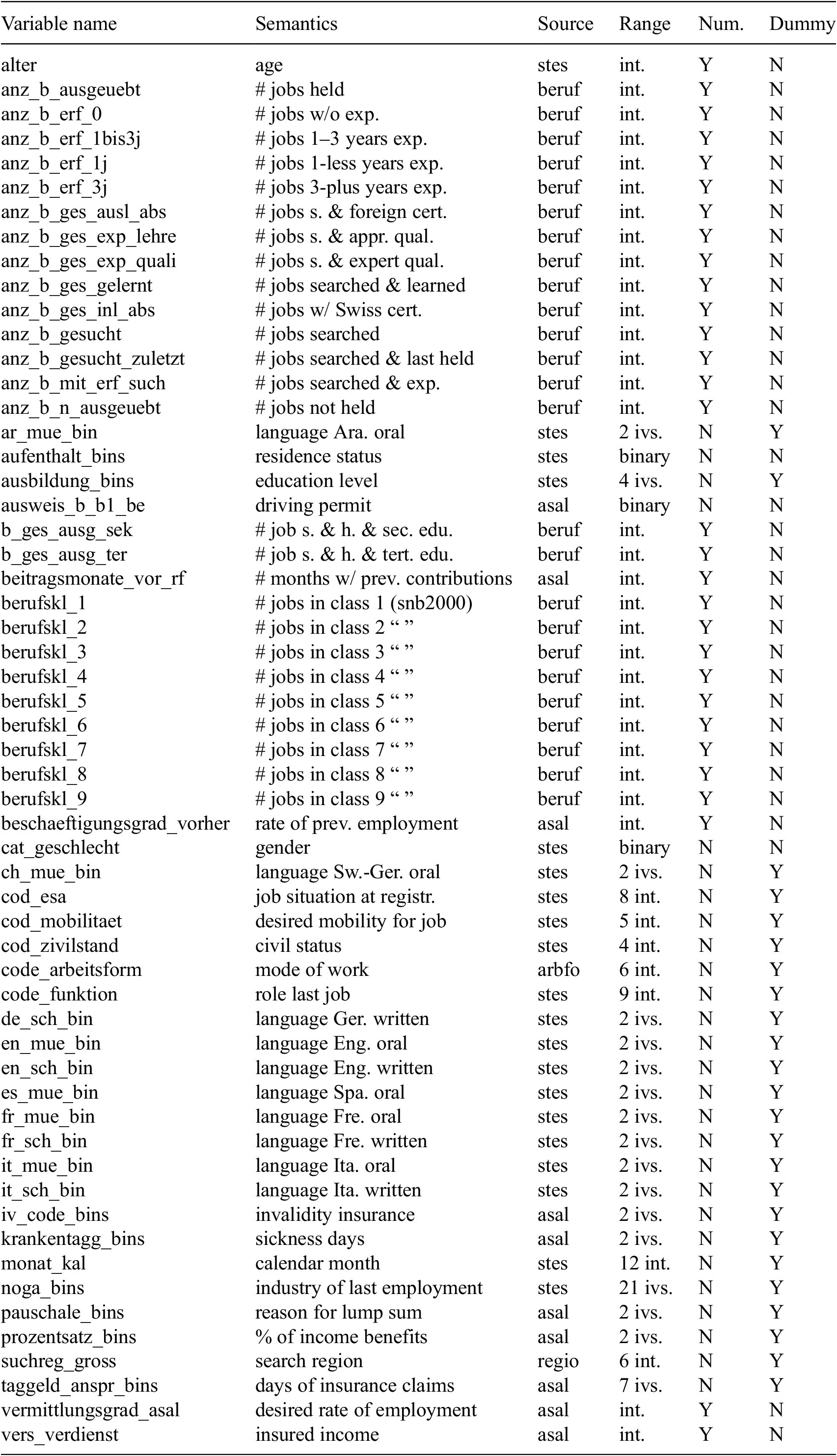
Table A1. Long description
The table contains 57 rows and 6 columns. The headers are Variable name, Semantics, Source, Range, Num. (Y or N), and Dummy (Y or N).
Key variables include:
* alter: age, source s t e s, integer range, Num. Y, Dummy N.
* anz_b_ausgeuebt: number of jobs held, source beruf, integer range, Num. Y, Dummy N.
* anz_b_erf_0 to anz_b_erf_3j: number of jobs with varying levels of experience (none, 1 to 3 years, less than 1 year, 3 plus years).
* anz_b_ges_ausl_abs: number of jobs searched and foreign certification.
* anz_b_ges_inl_abs: number of jobs with Swiss certification.
* ar_mue_bin: Arabic oral language, source s t e s, 2 intervals range, Num. N, Dummy Y.
* ausbildung_bins: education level, 4 intervals range, Num. N, Dummy Y.
* berufskl_1 to berufskl_9: number of jobs in Swiss job nomenclature 2000 classes 1 through 9.
* cat_geschlecht: gender, binary range, Num. N, Dummy N.
* ch_mue_bin: Swiss-German oral language.
* de_sch_bin: German written language.
* en_mue_bin and en_sch_bin: English oral and written language.
* fr_mue_bin and fr_sch_bin: French oral and written language.
* it_mue_bin and it_sch_bin: Italian oral and written language.
* noga_bins: industry of last employment, 21 intervals range.
* vers_verdienst: insured income, source a s a l, integer range, Num. Y, Dummy N.
Sources listed include s t e s, beruf, a s a l, regio, and arbfo. Ranges are primarily integers, binary, or specific intervals (ivs).
Note. For a description of “Source,” see raw data given earlier.
Abbreviations: appr.: apprenticeship; cert.: certification; empl.: employment; exp.: experience; h.: held; int.: integer; ins.: insurance; ivs.: intervals; lang.: language skills; mob.: mobility; qual.: qualification; registr.: registration; s.: searched; sbn2000: Swiss job nomenclature 2000 (publicly available via Swiss Federal Statistical Office.); sec.: secondary, Sw.Ger.: Swiss-German; tert.: tertiary.
B. Hyperparameters
Hyperparameter settings
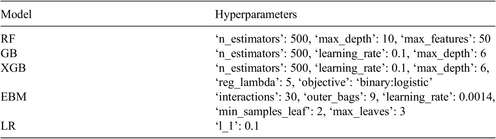
Table B1. Long description
The table contains two columns: Model and Hyperparameters.
* R F: n underscore estimators is 500, max underscore depth is 10, max underscore features is 50.
* G B: n underscore estimators is 500, learning underscore rate is 0.1, max underscore depth is 6.
* X G B: n underscore estimators is 500, learning underscore rate is 0.1, max underscore depth is 6, reg underscore lambda is 5, objective is binary logistic.
* E B M: interactions is 30, outer underscore bags is 9, learning underscore rate is 0.0014, min underscore samples underscore leaf is 2, max underscore leaves is 3.
* L R: l underscore 1 is 0.1.
For XGB and EBM, hyperparameter search was performed using the Optuna package (Akiba et al., Reference Akiba, Sano, Yanase, Ohta and Koyama2019), a state-of-the-art hyperparameter tuning framework. We thus get a “fair” comparison of the best black-box and the best interpretable model. For XGB, 50 trials in Optuna over all folds and available hyperparameters did not yield a substantive gain in AUC, with a best average AUC of 0.7743; it was therefore decided to retain the original parameters. For EBM, it was found that the main hyperparameter affecting performance was the number of interactions, with a higher number of interactions leading to better performance. It was decided to set the number of interactions to a (low) value by hand, because the main goal was to obtain an interpretable version of EBM, which includes limiting the number of features and interactions. Thus, effectively, hyperparameter tuning was only used for EBM. Additionally, EBM hyperparameters were not optimized for performance exclusively. Note that hyperparameter tuning is relatively cheap for XGB, but expensive for EBM, because the latter model is much slower to fit. Hyperparameters were not tuned for RF and GB; values were taken from Gasser (Reference Gasser2022), who optimized these models on the same data, but in a different context.
C. Additional results
C.1. Predictive performance
Results (AUC) by validate year (2015–2018) and test year (2019)
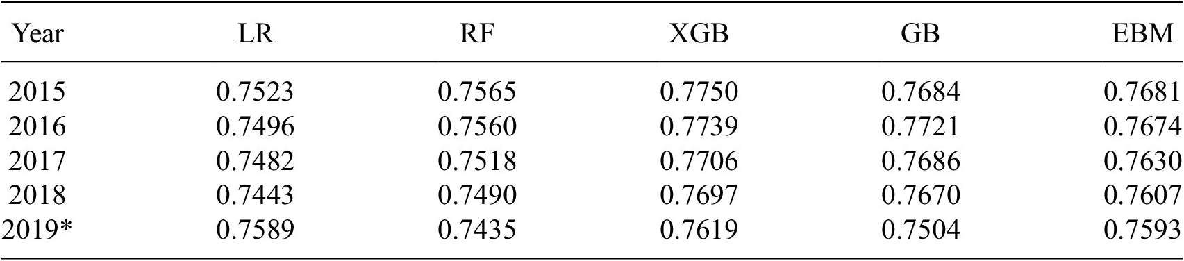
Table C1. Long description
The table consists of six columns and six rows. The columns are labeled Year, L R, R F, X G B, G B, and E B M.
* Row 1, Year 2015: L R 0.7523, R F 0.7565, X G B 0.7750, G B 0.7684, E B M 0.7681.
* Row 2, Year 2016: L R 0.7496, R F 0.7560, X G B 0.7739, G B 0.7721, E B M 0.7674.
* Row 3, Year 2017: L R 0.7482, R F 0.7518, X G B 0.7706, G B 0.7686, E B M 0.7630.
* Row 4, Year 2018: L R 0.7443, R F 0.7490, X G B 0.7697, G B 0.7670, E B M 0.7607.
* Row 5, Year 2019 asterisk: L R 0.7589, R F 0.7435, X G B 0.7619, G B 0.7504, E B M 0.7593.
The X G B model consistently shows the highest A U C values across the validation years 2015 to 2018.
Note. Results are displayed graphically in Figure 1.
C.2. Interpretability: sparsity
Effect of
$ {L}_1 $
 regularization on number of nonzero features and predictive performance of LR. Note that an AUC of 0.5 corresponds to random predictions (uninformative model).
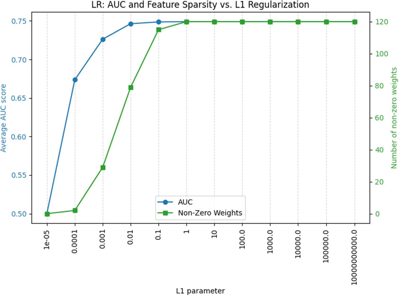
Figure C1. Long description
The graph is titled L R A U C and Feature Sparsity versus L 1 Regularization.
* The horizontal X axis represents the L 1 parameter on a logarithmic scale, ranging from 1 e minus 05 to 10000000000.0.
* The primary vertical Y axis on the left represents the Average A U C score, ranging from 0.50 to 0.75.
* The secondary vertical Y axis on the right represents the Number of non-zero weights, ranging from 0 to 120.
Two data series are plotted:
1. A U C (blue line with circular markers): Starts at 0.50 for an L 1 parameter of 1 e minus 05, shows a steep logarithmic increase to approximately 0.75 at an L 1 parameter of 0.1, and then plateaus at 0.75 for all subsequent values.
2. Non-Zero Weights (green line with square markers): Starts at 0 for an L 1 parameter of 1 e minus 05, remains near 0 until 0.0001, then increases sharply between 0.001 and 1. It reaches a maximum of 120 non-zero weights at an L 1 parameter of 1 and remains constant at 120 for all higher values.
A legend at the bottom center identifies the blue circles as A U C and the green squares as Non-Zero Weights.
Performance Score (AUC) for EBMs obtained from backward selection, retaining
$ n $
 most important main features in steps of 5. For each
$ n $
most important main features in steps of 5. For each
$ n $
 , a fraction of
$ 0.5 $
, a fraction of
$ 0.5 $
 interactions of the total number of main effects were added; the rightmost model, with 57 main features and 30 interactions, is the full EBM.

Figure C2. Long description
The x-axis is labeled Number of main features and ranges from 0 to 60 with major ticks every 10 units. The y-axis is labeled A U C Score and ranges from 0.740 to 0.765 with major ticks every 0.005.
Data points are represented by blue circles connected by a solid blue line. The trend shows a steep logarithmic increase in performance initially, followed by a plateau.
* At 5 features, the A U C is approximately 0.738.
* At 10 features, it rises sharply to 0.750.
* At 15 features, it reaches approximately 0.758.
* Between 20 and 35 features, the score continues to climb more gradually from 0.761 to 0.766.
* From 40 to 60 features, the performance plateaus, fluctuating slightly between 0.767 and 0.768, indicating diminishing returns as more features and interactions are added to the E B M.
Global explanation (feature importance plot) generated by EBM interface. It shows the (average) feature importance of the 15 most important features for fold 1 (trained on data from 2014). Features with “&” are interactions. See Table A1 for feature semantics.
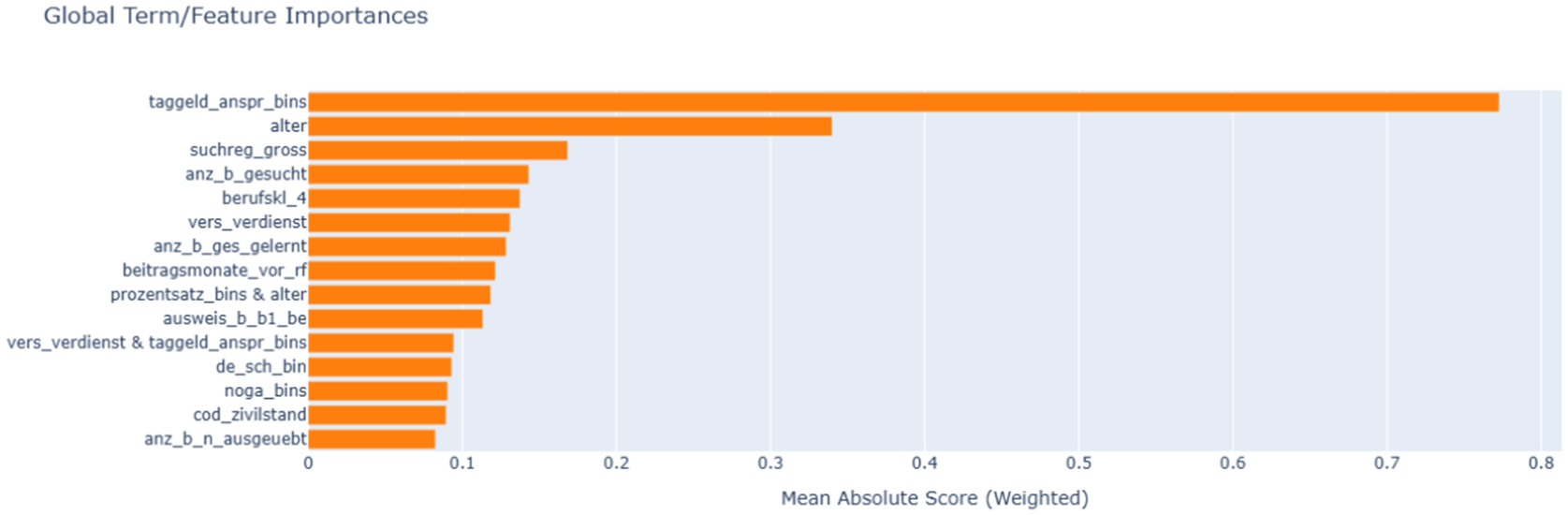
Figure C3. Long description
The horizontal axis represents the Mean Absolute Score weighted, ranging from 0 to 0.8 with grid lines every 0.1 units. The vertical axis lists 15 features. From top to bottom, the features and their approximate scores are.
* taggeld_anspr_bins at 0.78
* alter at 0.34
* suchreg_gross at 0.17
* anz_b_gesucht at 0.14
* berufskl_4 at 0.135
* vers_verdienst at 0.13
* anz_b_ges_gelernt at 0.125
* beitragsmonate_vor_rf at 0.12
* prozentsatz_bins ampersand alter at 0.115
* ausweis_b_b1_be at 0.11
* vers_verdienst ampersand taggeld_anspr_bins at 0.095
* de_sch_bin at 0.092
* noga_bins at 0.09
* cod_zivilstand at 0.088
* anz_b_n_ausgeuebt at 0.08
The top feature, taggeld_anspr_bins, shows a significantly higher importance score than all other features, more than double the second-ranked feature.
C.3. Interpretability: smoothing
Numerical feature “age” (alter), in raw version (off-the-shelf EBM) and after applying smoothing spline with smoothing parameter
$ \lambda $
 ; age in years.
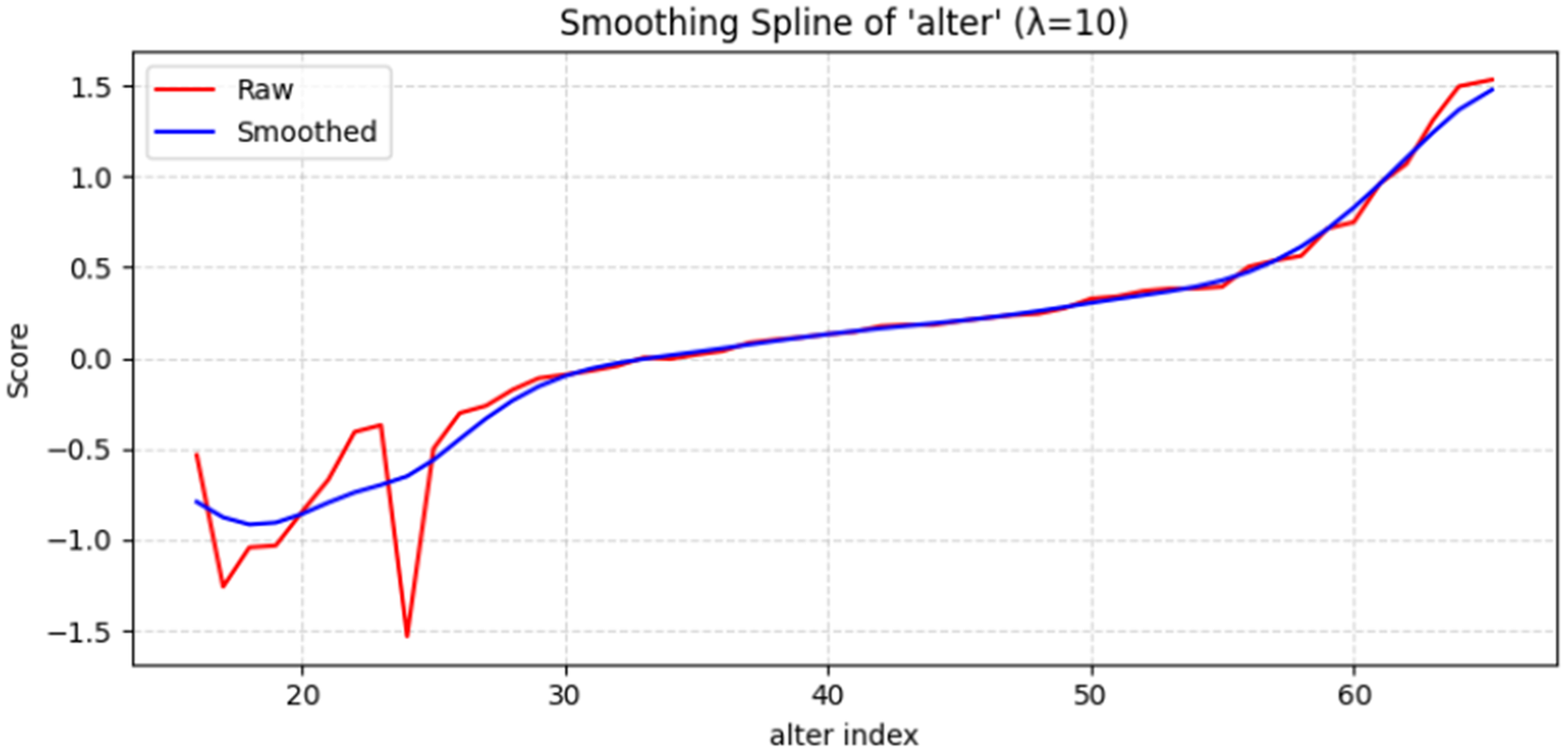
Figure C4. Long description
The graph is titled Smoothing Spline of ‘alter’ with lambda equals 10. The x-axis is labeled alter index and ranges from approximately 15 to 65. The y-axis is labeled Score and ranges from negative 1.5 to 1.5.
Two lines are plotted:
* A red line labeled Raw shows highly volatile fluctuations between alter index 15 and 25, including a sharp drop to negative 1.5 at index 24. From index 30 onward, it follows a steady upward trend with minor jaggedness, ending at a score of approximately 1.5.
* A blue line labeled Smoothed provides a continuous curve that averages the raw data. It begins with a shallow dip around index 18, then rises steadily. Between index 30 and 55, it shows a near-linear increase with a low slope. After index 55, the curve steepens, ending at a score of approximately 1.5 at index 65.
The smoothed line effectively removes the extreme noise seen in the early raw data while maintaining the overall sigmoidal growth pattern.
Numerical feature “number of months of previous contributions” (beitragsmonate_vor_rf), in raw version (off-the-shelf EBM) and after applying smoothing spline with smoothing parameter
$ \lambda $
 .
.
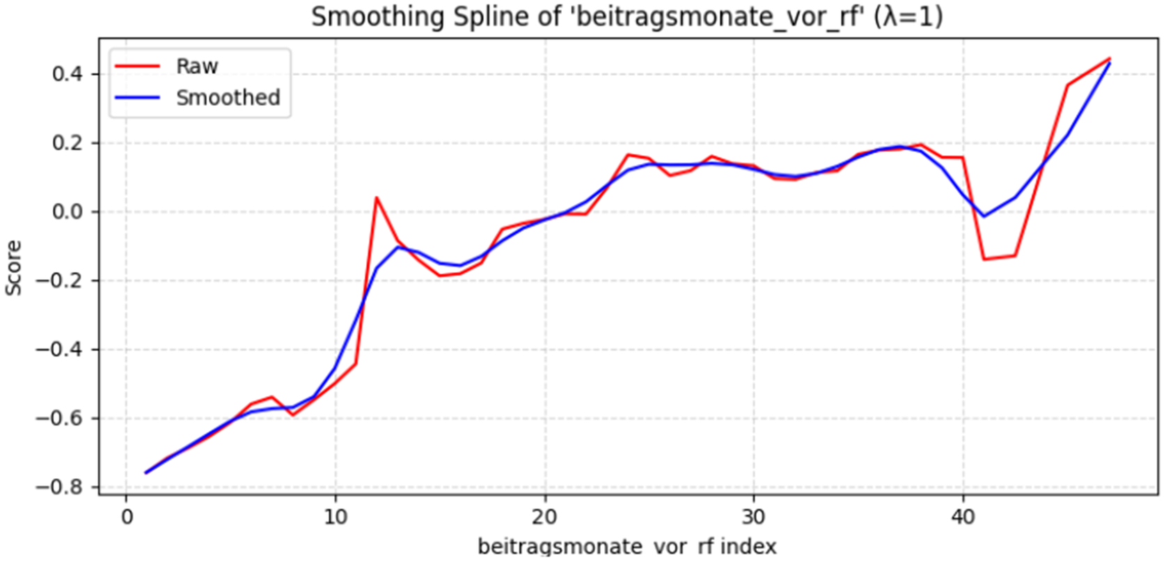
Figure C5. Long description
The graph features a horizontal X-axis labeled beitragsmonate underscore vor underscore r f index ranging from 0 to 50 and a vertical Y-axis labeled Score ranging from negative 0.8 to 0.4. A legend in the top-left corner identifies a red line as Raw and a blue line as Smoothed.
* The Raw red line shows high volatility with sharp peaks and troughs. It starts at negative 0.75, rises steadily to negative 0.45 at index 10, then spikes sharply to 0.05 at index 12. It fluctuates between negative 0.2 and 0.2 across the middle section before dropping sharply to negative 0.15 at index 41 and finally rising to 0.45 at index 47.
* The Smoothed blue line follows the same general upward trajectory but filters out the sharp noise. It uses a smoothing spline with lambda equals 1 to create a continuous curve that averages the Raw data’s fluctuations, particularly visible in the plateau between index 25 and 40 where it maintains a steady wave-like pattern around the 0.1 score mark.
* Both lines converge at the start and end points of the dataset.
Numerical feature “rate of desired employment” (vermittlungsgrad_asal), in raw version (off-the-shelf EBM) and after applying smoothing spline with smoothing parameter
$ \lambda $
 .
.
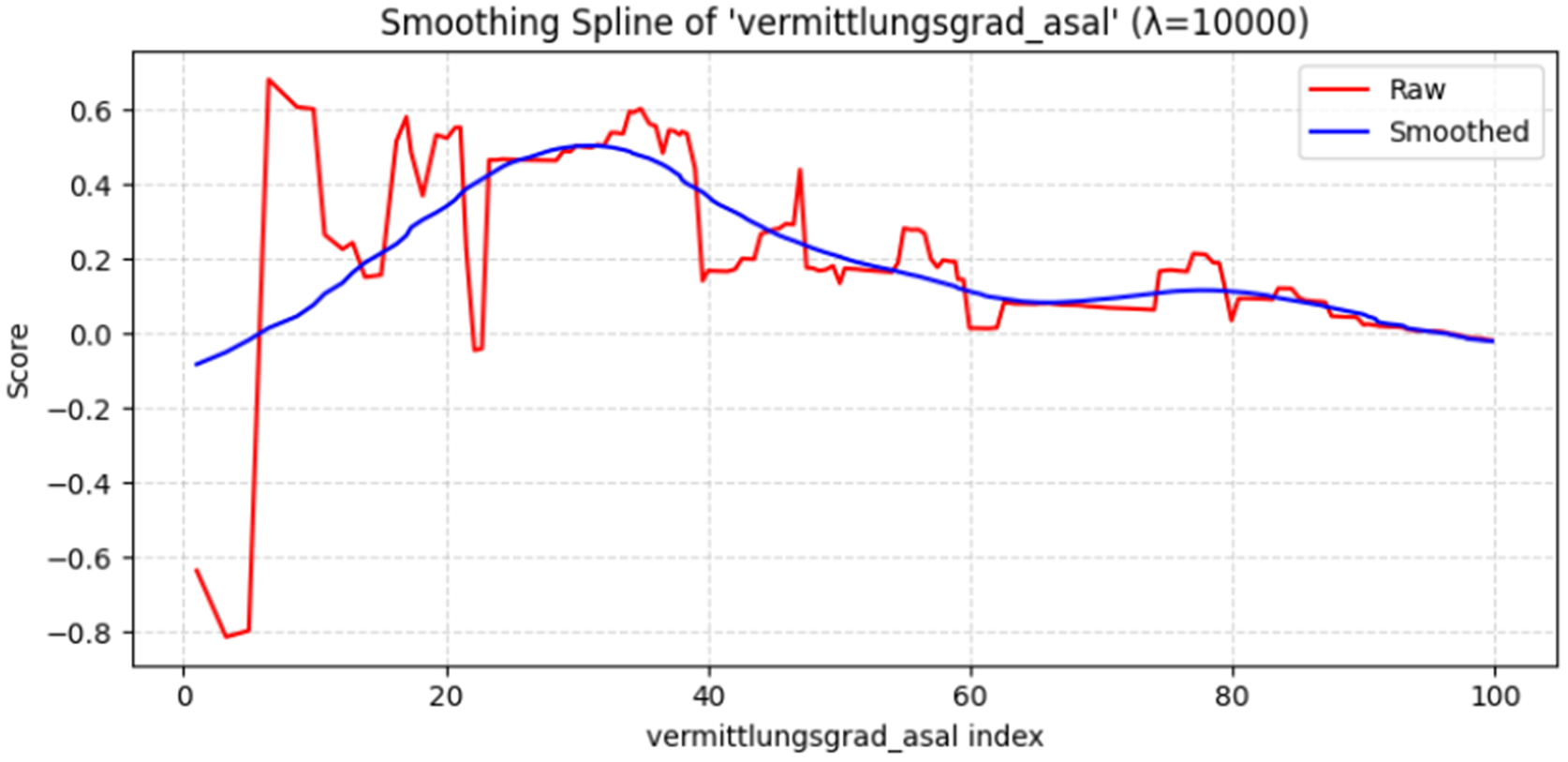
Figure C6. Long description
The graph is titled Smoothing Spline of vermittlungsgrad underscore asal with lambda equal to 10000. The horizontal x-axis is labeled vermittlungsgrad underscore asal index and ranges from 0 to 100. The vertical y-axis is labeled Score and ranges from negative 0.8 to 0.6. A legend in the top right identifies two data series.
* The Raw data, shown as a jagged red line, begins at a score of negative 0.6, drops to negative 0.8, then spikes sharply to 0.6 before fluctuating wildly between 0.0 and 0.6 until index 40. After index 40, it shows a general downward trend with smaller oscillations, ending near 0.0.
* The Smoothed data, shown as a solid blue line, provides a continuous curve that filters out the noise of the red line. It starts at negative 0.1, rises steadily to a peak of 0.5 at index 30, and then gradually descends in a smooth wave-like motion, converging with the raw data at index 100.
The grid consists of light gray dashed lines.
C.4. Interpretability: local explanation
Example of a local explanation generated by EBM interface for a full EBM. Fictitious example with random features and outcome. Contributions of single features and interactions (two features connected by “&”) to overall risk score are ordered in descending absolute importance; blue features contribute negatively (lower score), orange features contribute positively (higher score). Only 15 most important features and intercept (fixed) are listed. See Table A1 for feature semantics.
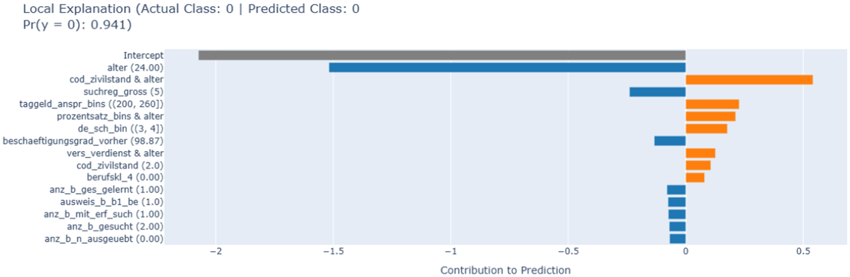
Figure C7. Long description
The chart is titled Local Explanation with Actual Class 0, Predicted Class 0, and a probability of y equals 0 at 0.941. The x-axis is labeled Contribution to Prediction with a scale from negative 2 to positive 0.5.
From top to bottom, the features are:
* Intercept: A long grey bar extending to negative 2.1.
* alter 24.00: A blue bar extending to negative 1.5.
* cod underscore zivilstand and alter: A long orange bar extending to positive 0.55.
* suchreg underscore gross 5: A blue bar extending to negative 0.25.
* taggeld underscore anspr underscore bins 200, 260: An orange bar extending to positive 0.22.
* prozentsatz underscore bins and alter: An orange bar extending to positive 0.21.
* de underscore sch underscore bin 3, 4: An orange bar extending to positive 0.18.
* beschaeftigungsgrad underscore vorher 98.87: A blue bar extending to negative 0.15.
* vers underscore verdienst and alter: An orange bar extending to positive 0.12.
* cod underscore zivilstand 2.0: An orange bar extending to positive 0.10.
* berufskl underscore 4 0.00: An orange bar extending to positive 0.08.
* anz underscore b underscore ges underscore gelernt 1.00: A blue bar extending to negative 0.05.
* ausweis underscore b underscore b1 underscore be 1.0: A blue bar extending to negative 0.05.
* anz underscore b underscore mit underscore erf underscore such 1.00: A blue bar extending to negative 0.05.
* anz underscore b underscore gesucht 2.00: A blue bar extending to negative 0.05.
* anz underscore b underscore n underscore ausgeuebt 0.00: A blue bar extending to negative 0.05.
C.5. Fairness
Cumulative gain curve for EBM-30 model. This curve can serve as a basis for the choice of threshold. In the hypothetical fairness scenario, a level of positive cases to be captured (80%) was chosen; one can then read off the cumulative gains curve that in this case, one has to target approximately 49% of the total population.
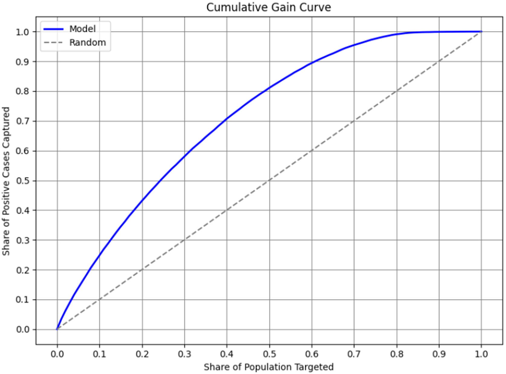
Performance metrics of group intersections, before (a) and after (b) fairness mitigation.
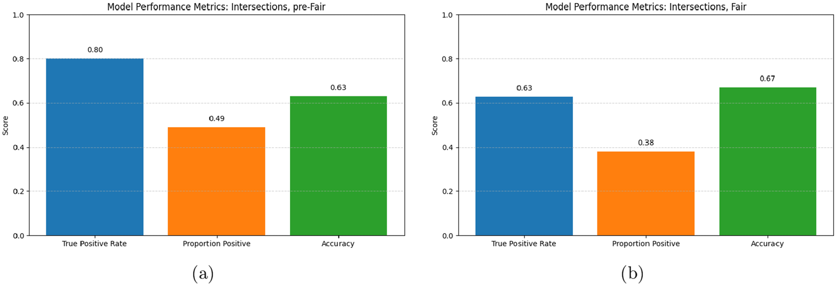
Confusion matrices (normalized) for 12 group intersections, before fairness mitigation. Age groups: 15–29, 30–44, 45–65; gender: female, male; residency status: nonpermanent residents, permanent residents.
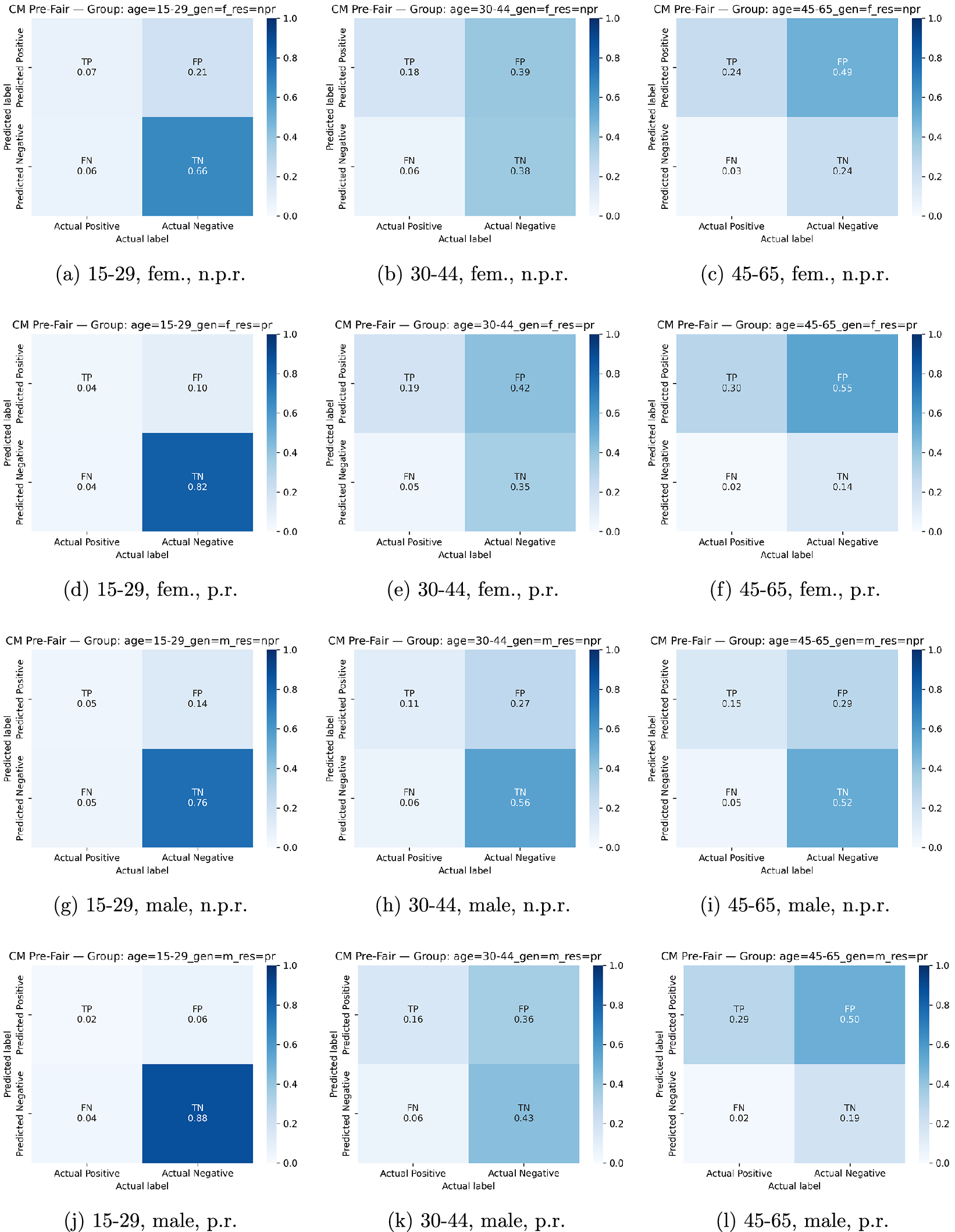
Figure C10. Long description
A grid of 12 normalized confusion matrices labeled a through l. Each matrix has an x-axis for Actual label (Actual Positive, Actual Negative) and a y-axis for Predicted label (Predicted Positive, Predicted Negative). A color scale on the right of each plot ranges from 0.0 (light blue) to 1.0 (dark blue).
Row 1: Female, nonpermanent residents (n p r).
* a. Age 15-29: T P 0.07, F P 0.21, F N 0.06, T N 0.66.
* b. Age 30-44: T P 0.18, F P 0.39, F N 0.06, T N 0.38.
* c. Age 45-65: T P 0.24, F P 0.49, F N 0.03, T N 0.24.
Row 2: Female, permanent residents (p r).
* d. Age 15-29: T P 0.04, F P 0.10, F N 0.04, T N 0.82.
* e. Age 30-44: T P 0.19, F P 0.42, F N 0.05, T N 0.35.
* f. Age 45-65: T P 0.30, F P 0.55, F N 0.02, T N 0.14.
Row 3: Male, nonpermanent residents (n p r).
* g. Age 15-29: T P 0.05, F P 0.14, F N 0.05, T N 0.76.
* h. Age 30-44: T P 0.11, F P 0.27, F N 0.06, T N 0.56.
* i. Age 45-65: T P 0.15, F P 0.29, F N 0.05, T N 0.52.
Row 4: Male, permanent residents (p r).
* j. Age 15-29: T P 0.02, F P 0.06, F N 0.04, T N 0.88.
* k. Age 30-44: T P 0.16, F P 0.36, F N 0.06, T N 0.43.
* l. Age 45-65: T P 0.29, F P 0.50, F N 0.02, T N 0.19.
Across all groups, the True Negative (T N) rate is highest in the 15-29 age group and lowest in the 45-65 age group, while False Positive (F P) rates increase with age.
Confusion matrices (normalized) for 12 group intersections, after fairness mitigation. Age groups: 15–29, 30–44, 45–65; gender: female, male; residency status: nonpermanent residents, permanent residents.
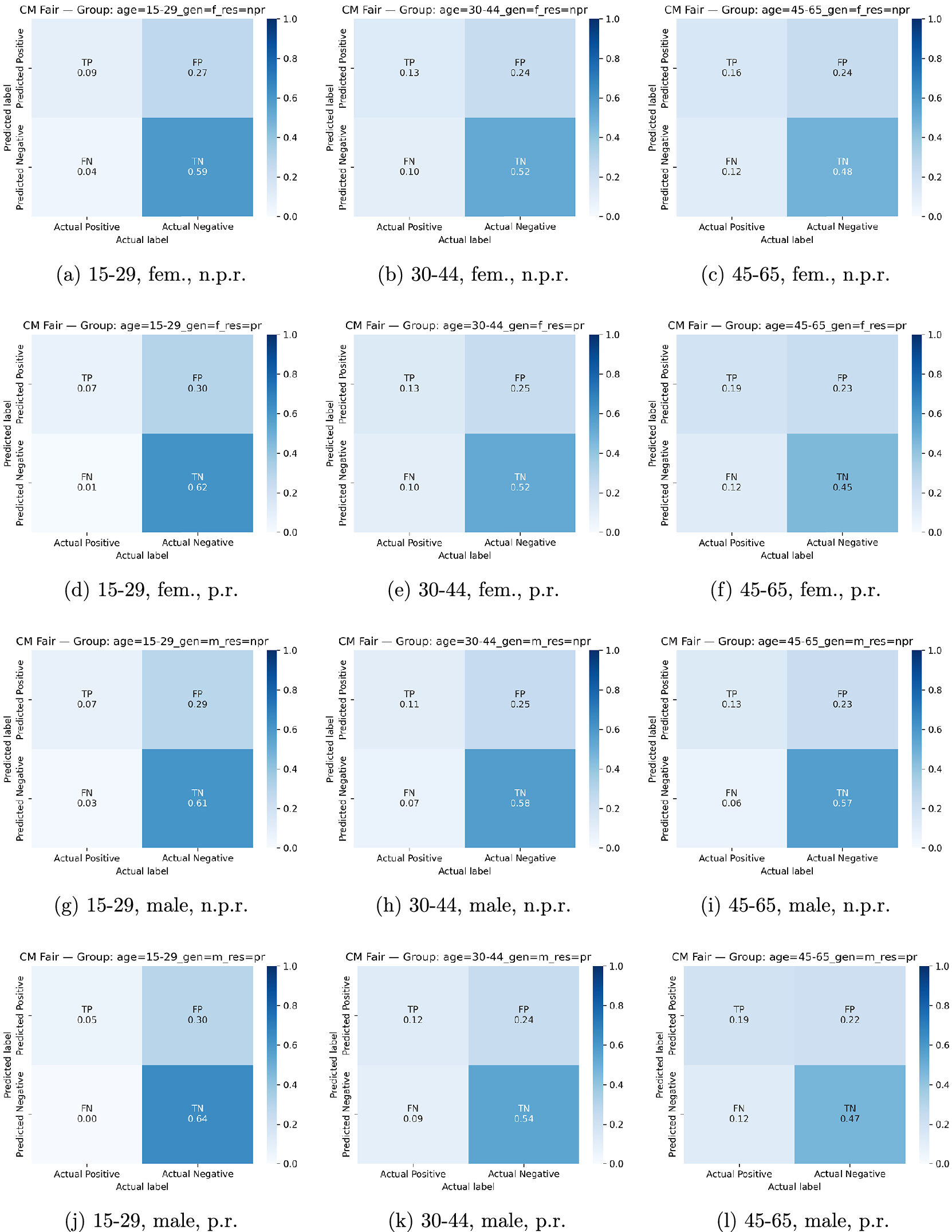
Figure C11. Long description
Twelve heatmaps are arranged in a grid. Each heatmap has an x-axis labeled Actual label with categories Actual Positive and Actual Negative, and a y-axis labeled Predicted label with categories Predicted Positive and Predicted Negative. A color scale on the right of each panel ranges from 0.0 to 1.0 in shades of blue. Each panel contains four values: T P (top-left), F P (top-right), F N (bottom-left), and T N (bottom-right).
Row 1: Female, nonpermanent residents (n p r).
* Panel a (15-29): T P 0.09, F P 0.27, F N 0.04, T N 0.59.
* Panel b (30-44): T P 0.13, F P 0.24, F N 0.10, T N 0.52.
* Panel c (45-65): T P 0.16, F P 0.24, F N 0.12, T N 0.48.
Row 2: Female, permanent residents (p r).
* Panel d (15-29): T P 0.07, F P 0.30, F N 0.01, T N 0.62.
* Panel e (30-44): T P 0.13, F P 0.25, F N 0.10, T N 0.52.
* Panel f (45-65): T P 0.19, F P 0.23, F N 0.12, T N 0.45.
Row 3: Male, nonpermanent residents (n p r).
* Panel g (15-29): T P 0.07, F P 0.29, F N 0.03, T N 0.61.
* Panel h (30-44): T P 0.11, F P 0.25, F N 0.07, T N 0.58.
* Panel i (45-65): T P 0.13, F P 0.23, F N 0.06, T N 0.57.
Row 4: Male, permanent residents (p r).
* Panel j (15-29): T P 0.05, F P 0.30, F N 0.00, T N 0.64.
* Panel k (30-44): T P 0.12, F P 0.24, F N 0.09, T N 0.54.
* Panel l (45-65): T P 0.19, F P 0.22, F N 0.12, T N 0.47.

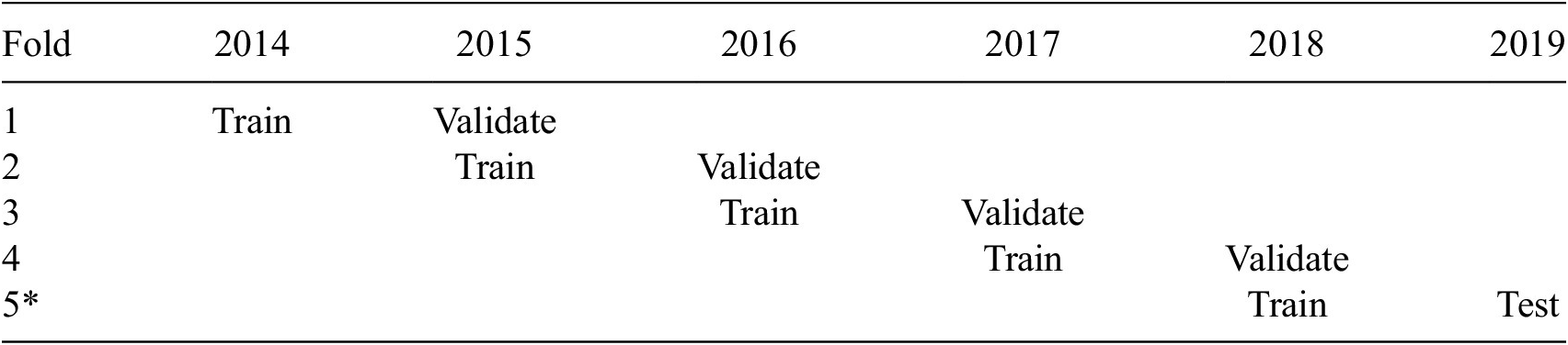
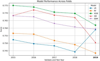
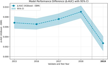
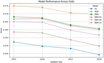
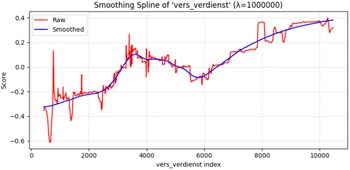

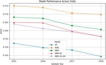
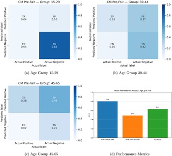
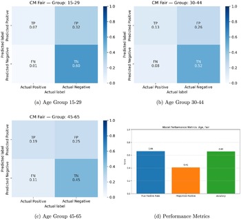
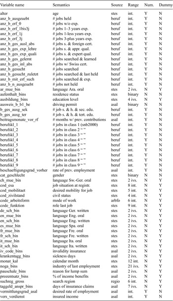
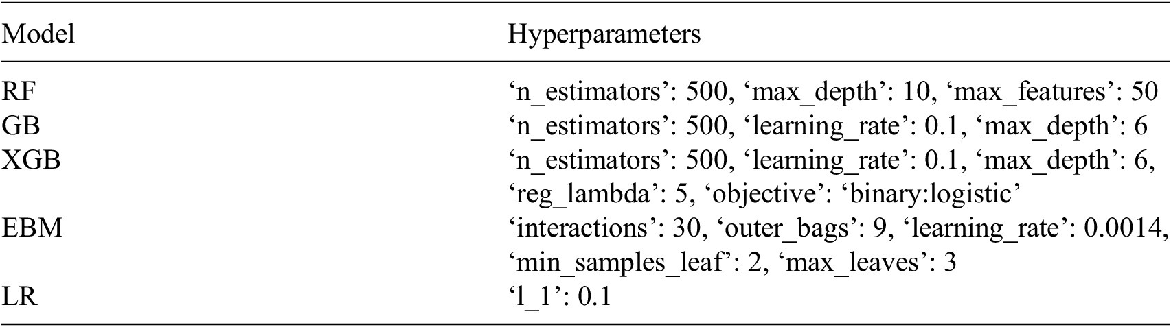
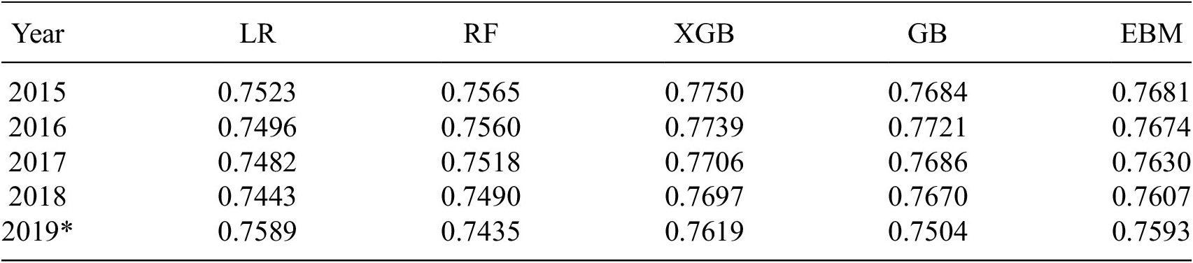
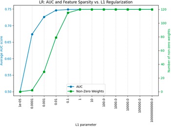

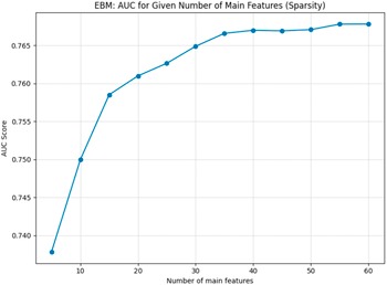


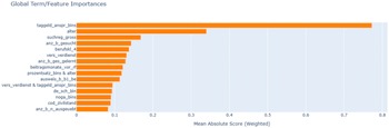
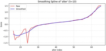

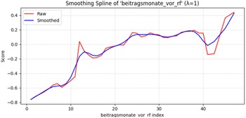

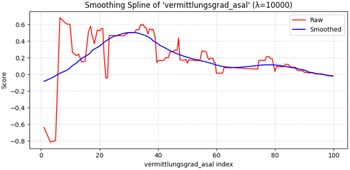

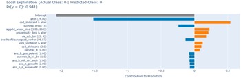

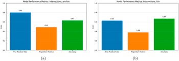
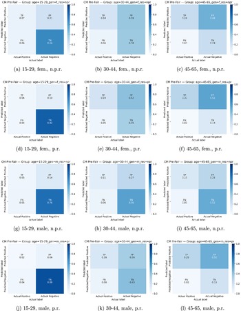


 Open access


Comments
No Comments have been published for this article.