





1. Background
Design and innovation processes fundamentally involve generating knowledge through the retrieval and synthesis of the knowledge of existing technological artifacts (Liu, Tao, & Bi Reference Liu, Tao and Bi2022). Ontologies explicitly specify how knowledge is conceptualized in a domain of discourse (Gruber Reference Gruber1993; Chandrasegaran et al. Reference Chandrasegaran, Ramani, Sriram, Horváth, Bernard, Harik and Gao2013). They have been central to engineering design research in knowledge retrieval and representation, where scholars theorize and operationalize the basis of knowledge represented, retrieved and reused during design and innovation processes (Siddharth, Blessing, & Luo Reference Siddharth, Blessing and Luo2022a). Their contributions stem from different perspectives, such as:
-
• The systems engineering perspective (Simon Reference Simon1962) suggests that artifacts constitute various parts that interact in different ways – largely involving material, energy and information exchanges via shared interfaces (Browning Reference Browning2001) – such that the whole is more than the sum of its parts.
-
• The function structure perspective (Rodenacker & Rodenacker Reference Rodenacker, Rodenacker and Rodenacker1976) simplifies the overall function of a technological artifact into sub-functions that are connected using flows, represented using a prescribed vocabulary (Hirtz et al. Reference Hirtz, Stone, McAdams, Szykman and Wood2002) for both functions (for example, import and transfer) and flows (for example, liquid and signal).
-
• The qualitative physics perspective (De Kleer & Brown Reference De Kleer and Brown1984) describes an artifact using constructs such as structure (what?), behavior (how?) and purpose (why?), leading to various theories and models on functional representation (Chandrasekaran & Josephson Reference Chandrasekaran and Josephson2000).
-
• The Core Product Model (Fenves et al. Reference Fenves, Foufou, Bock and Sriram2008) developed at the National Institute of Standards and Technology (NIST) integrates these perspectives into a scheme having object (for example, geometry, material) and relationship (for example, constraint, part-of) classes.
In technology and innovation management fields as well, scholars theorize the foundations of the knowledge of technological artifacts. Herein, scholars study the knowledge of technological domains to understand the mechanisms of technological change. They capture domain-level knowledge using networks of topics, co-inventors, co-classifications, co-assignees and co-citations, predominantly populated from patent databases (Siddharth, Li, & Luo Reference Siddharth, Li and Luo2022b; Li, Siddharth, & Luo Reference Li, Siddharth and Luo2023). For instance, Malhotra et al. (Reference Malhotra, Zhang, Beuse and Schmidt2021) assess the citation network of 101,260 patents under lithium-ion batteries and find 491 patents forming the core of the network and governing the knowledge trajectory.
These perspectives only reflect expert views on how the knowledge of an artifact should be systematically captured. Robinson et al. (2023) studied the sewing machine patents granted in the last 200 years to model the “dominant” functional architecture using techniques proposed in the functional basis (Hirtz et al. Reference Hirtz, Stone, McAdams, Szykman and Wood2002), leveraging an expert-defined ontological lens to study the domain of interest. In addition, the studies in technology management seem to rely on meta-level knowledge given by citations, inventors, classifications and others, which themselves represent an expert-defined scheme of technology space, without considering the actual knowledge of artifacts documented in vast text documents (Siddharth et al., Reference Siddharth, Blessing and Luo2022a, Reference Siddharth, Blessing, Wood and Luo2021). Considering these broad research gaps, we address the following research question from a different perspective.
What is the basis of the knowledge of technological artifacts? To address the above, we procure the knowledge of technological artifacts from a large sample of patent descriptions. Specifically, we populate knowledge graphs of patent descriptions using the sentence-level fact extraction methods developed in our prior work (Siddharth & Luo Reference Siddharth and Luo2024; Siddharth Reference Siddharth2024a). Using the knowledge graphs, we implement techniques from computational linguistics and networks to reveal the linguistic and structural foundations of the knowledge of technological artifacts. By leveraging patent descriptions (not the metadata) and bottom-up (not expert-defined), sentence-level fact extraction for populating knowledge graphs, our study addresses the overall research gaps observed in both engineering design and technology management literature.
2. Data and methods
2.1. Knowledge graph data
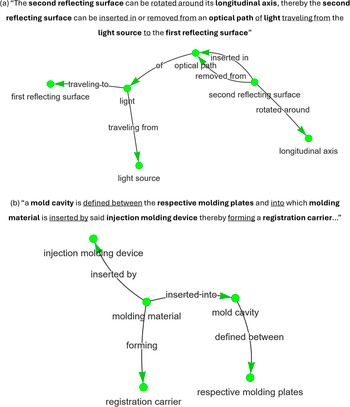
Patent documents offer rich and detailed descriptions of several million technological artifacts spanning the total technology space (Siddharth, Li, & Luo Reference Siddharth, Li and Luo2022b). Despite this advantage, patent documents remain underutilized due to the lack of methods to explicitly capture the knowledge structures of artifacts representing them. To address this limitation, we recently developed a method (Siddharth & Luo Reference Siddharth and Luo2024; Siddharth Reference Siddharth2024a) to extract sentence-level facts of the form entity:: relationship:: entity from patent documents. The following is an example of facts extracted from a sentence taken from a glue gun patentFootnote 1.
“The adhesive, softened by the heating step, can be readily extruded mechanically by means of a piston from the front end of the glue gun.”
The adhesive:: softened by:: the heating step
The adhesive:: readily extruded mechanically by:: means
means:: of:: a piston
means:: from:: the front end
a piston:: from:: the front end
the front end:: of:: the glue gun
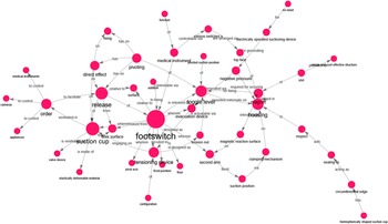
Exhibiting up to 99.7% accuracy, the method for extracting facts – as illustrated above – relies on a two-stage transformer-based language model trained on a proprietary dataset of 50,000 patent sentences and factsFootnote 2. Applying this method sentence-wise to a patent description results in a list of facts that can be combined into a knowledge graph, as illustrated in Figure 1. We utilize our prior method to populate knowledge graphs – illustrated further in Figure 2 – of a large sample of patent descriptions and utilize these knowledge graphs to study the foundations of the knowledge of technological artifacts. To gather the sample of patents, we leverage Patents ViewFootnote 3 and source patent information as of 8 June 2023, by which the database included over 8.2 million granted US patents. We restrict our scope to utility patents that are granted for their functionalities rather than aesthetics or other criteria.
Illustrating explication of knowledge using a sentence from patented artifact descriptions of (a) vehicle light (Vehicle light with movable reflector portion and shutter portion for selectively switching an illuminated area of light incident on a predetermined portion of the vehicle light during driving – https://patents.google.com/patent/US6796696/) and (b) injection molding (Installation for manufacturing registration carriers – https://patents.google.com/patent/US5451155/).
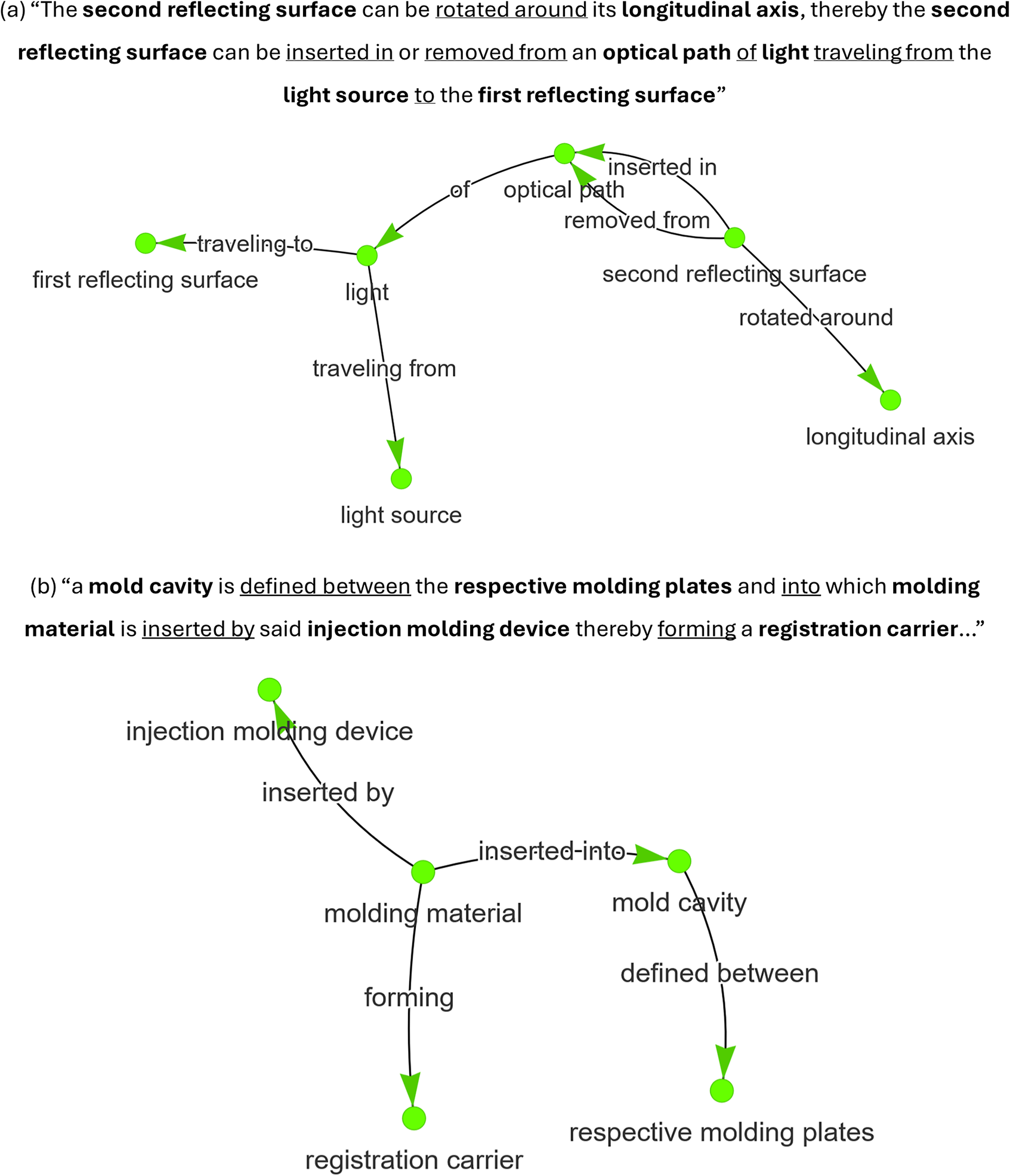
Figure 1. Long description
The upper panel maps a sentence about a vehicle light. Starting at the top left, ‘first reflecting surface’ connects via an arrow labeled ‘traveling-to’ to ‘light’, which connects downward to ‘light source’ via ‘traveling from’. From ‘light’, an arrow labeled ‘of’ leads rightward to ‘optical path’, which branches to ‘inserted in’ and ‘removed from’, both pointing to ‘second reflecting surface’. From there, an arrow labeled ‘rotated around’ points to ‘longitudinal axis’. The lower panel maps a sentence about injection molding. At the top left, ‘injection molding device’ connects downward via ‘inserted by’ to ‘molding material’. From ‘molding material’, an arrow labeled ‘forming’ points downward to ‘registration carrier’. ‘Molding material’ also connects rightward via ‘inserted-into’ to ‘mold cavity’, which connects downward via ‘defined between’ to ‘respective molding plates’.
Example knowledge graph extracted from a patent (Footswitch for a medical instrument – https://patents.google.com/patent/US10437277B2/) using our prior method (Siddharth & Luo Reference Siddharth and Luo2024). Each of the 33,881 patents in the sample data has a knowledge graph as illustrated here.
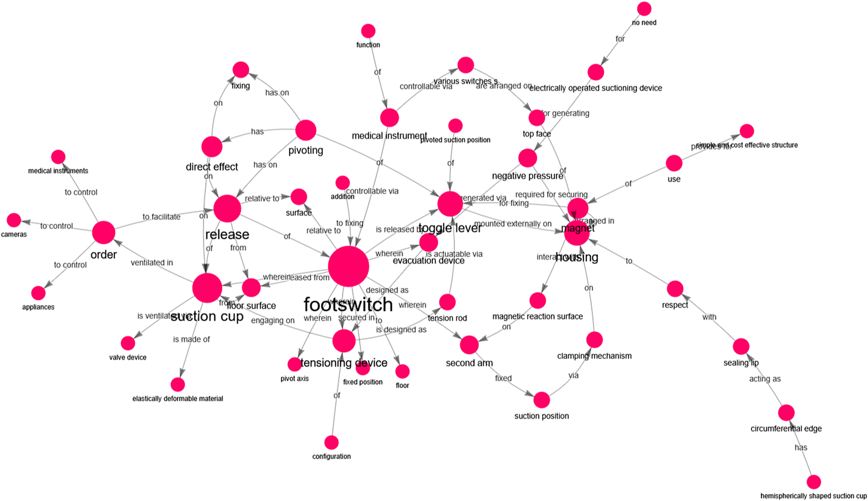
Figure 2. Long description
At the center is the largest node labeled ‘footswitch’. Directly connected are ‘toggle lever’, ‘release’, ‘suction cup’, ‘tensioning device’, ‘housing’, and ‘order’. Each of these nodes branches outward: ‘toggle lever’ links to ‘negative pressure’, ‘magnet’, ‘medical instrument’, and ‘pivoting’. ‘Release’ connects to ‘direct effect’, ‘surface’, and ‘relative to’. ‘Suction cup’ links to ‘valve device’, ‘elastically deformable material’, and ‘floor surface’. ‘Tensioning device’ connects to ‘pivot axis’, ‘fixed position’, and ‘configuration’. ‘Housing’ branches to ‘magnet’, ‘clamping mechanism’, ‘sealing lip’, and ‘circumferential edge’. ‘Order’ connects to ‘medical instruments’, ‘cameras’, and ‘appliances’. Arrows indicate functional or structural relationships, such as ‘is made of’, ‘is released from’, ‘is actuated via’, ‘is ventilated in’, and ‘is designed as’. Peripheral nodes include ‘function’, ‘use’, and ‘cost effective structure’, each connected by labeled arrows to relevant device features. The diagram visually maps the hierarchical and functional relationships among components and concepts related to the footswitch device.
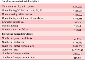
Considering the 7.3 million utility patents in the population, we use a Qualtrics calculatorFootnote 4 to determine a reasonable sample size of 16,540 according to a 99% confidence level and 1% margin of error. The calculator leverages the Cochran’s formula (Ahmed Reference Ahmed2024, p. 5) as shown in Equations 1 and 2.


Where
$ {N}_o $
 is the initial sample size calculated using the Z-score (
$ Z $
is the initial sample size calculated using the Z-score (
$ Z $
 ), Error (
$ E $
), Error (
$ E $
 ) and p-value (
$ p $
) and p-value (
$ p $
 ). Given the 1% margin of error, E is 0.01 –
$ Z $
). Given the 1% margin of error, E is 0.01 –
$ Z $
 is assigned 2.576 corresponding to 99% confidence value and p is assigned 0.5 as the default. The resulting
$ {N}_o $
is assigned 2.576 corresponding to 99% confidence value and p is assigned 0.5 as the default. The resulting
$ {N}_o $
 is adjusted for our population size,
$ {N}_P $
is adjusted for our population size,
$ {N}_P $
 = 7,373,519 (see Table 1), as in Equation 2. The final sample size, as per the calculation above, is returned as 16,540, subject to numerical approximations in the Qualtrics calculator. We intended the sample to be stratified according to patent counts as per the CPC 4-digit classification schemeFootnote
5 (for example, A02F). By constraining the distribution such that there is no overlap among classes, we obtain a sample of 33,945 patents (Table 1). For the sample of 33,945 patents, full text is available for 33,884 patents, which we clean and split into sentencesFootnote
6. For each sentence in each patent, we apply our method (Siddharth & Luo Reference Siddharth and Luo2024; Siddharth Reference Siddharth2024a) to extract facts of the form head entity:: relationship:: tail entity. When these facts are combined across sentences and within a patent, a knowledge graph can be obtained, as illustrated in Figure 2. The knowledge graph data populatedFootnote
7 for this work, including patent information, knowledge graphs and analysis, is publicly available (Siddharth Reference Siddharth2024b).
= 7,373,519 (see Table 1), as in Equation 2. The final sample size, as per the calculation above, is returned as 16,540, subject to numerical approximations in the Qualtrics calculator. We intended the sample to be stratified according to patent counts as per the CPC 4-digit classification schemeFootnote
5 (for example, A02F). By constraining the distribution such that there is no overlap among classes, we obtain a sample of 33,945 patents (Table 1). For the sample of 33,945 patents, full text is available for 33,884 patents, which we clean and split into sentencesFootnote
6. For each sentence in each patent, we apply our method (Siddharth & Luo Reference Siddharth and Luo2024; Siddharth Reference Siddharth2024a) to extract facts of the form head entity:: relationship:: tail entity. When these facts are combined across sentences and within a patent, a knowledge graph can be obtained, as illustrated in Figure 2. The knowledge graph data populatedFootnote
7 for this work, including patent information, knowledge graphs and analysis, is publicly available (Siddharth Reference Siddharth2024b).
Sampling patents and extracting design knowledge from USPTO
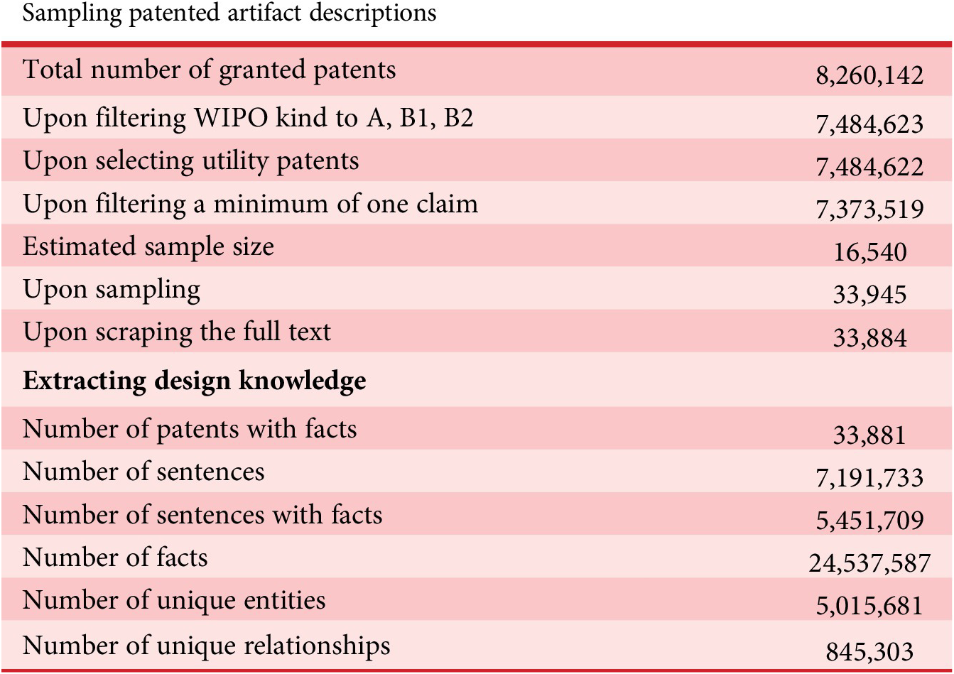
Table 1. Long description
The table is divided into two sections. The first section, Sampling patented artifact descriptions, lists sequential filtering steps with corresponding counts: total number of granted patents 8,260,142; upon filtering W I P O kind to A, B1, B2, 7,484,623; upon selecting utility patents, 7,484,622; upon filtering a minimum of one claim, 7,373,519; estimated sample size, 16,540; upon sampling, 33,945; upon scraping the full text, 33,884. The second section, Extracting design knowledge, includes: number of patents with facts, 33,881; number of sentences, 7,191,733; number of sentences with facts, 5,451,709; number of facts, 24,537,587; number of unique entities, 5,015,681; number of unique relationships, 845,303. Each value is aligned with its respective filtering or extraction step, proceeding from the top row downward.
2.2. Linguistic foundations – Zipf distribution analysis
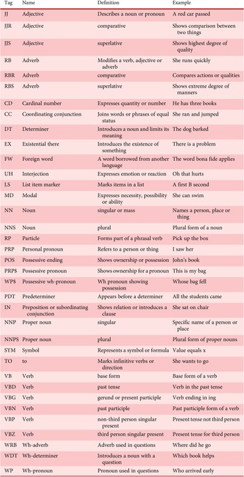
By studying the entities and relationships that form the knowledge graphs (for example, Figure 2), we uncover the linguistic foundations of the knowledge of technological artifacts. In Table 1, we noted that the 33,881 patent knowledge graphs together comprise 5,015,681 unique entities and 845,303 unique relationships. To understand how these entities and relationships are linguistically constructed, we transform them into syntaxesFootnote 8, for example, “a shake” ➔ “a NN,” “the cured spar assembly” ➔ “the JJ NNP NNP,” “all three erase blocks” ➔ “all CD NN NNS,” where the parts-of-speech NN = Noun, JJ = adjective, CD = cardinal number and others. In Appendix A, we provide the full list of parts of speech, their definitions and examples.
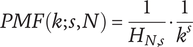
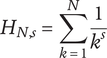
Upon transforming the terms that constitute patent knowledge graphs, we obtain 408,323 unique entity syntaxes and 73,352 unique relationship syntaxes. We analyze the frequencies of the unique syntaxes to find the most generalizable ones that form the linguistic foundations of the knowledge of technological artifacts. In computational linguistics, term frequencies in a corpus are typically studied using the Zipf distribution (Mollica & Piantadosi Reference Mollica and Piantadosi2019). In engineering design literature, Murphy et al. (Reference Murphy, Fu, Otto, Yang, Jensen and Wood2014) analyze 65,000 patent abstracts using Zipf distribution to identify the most representative 1,700 functions (verbs) of patented artifacts. Zipf distribution follows the probability mass function (PMF) as shown in Equations 3 and 4.
In the above equations,
$ N $
 is the number of distinct items, k stands for the rank of an item in the frequency distribution and s is the distribution parameter. The idea behind the Zipf distribution is that the probability of an item in the corpus is inversely related to its rank – k raised to the power – s. To ensure the probabilities of all terms sum to 1, a generalized harmonic number (
$ {H}_{N,s} $
is the number of distinct items, k stands for the rank of an item in the frequency distribution and s is the distribution parameter. The idea behind the Zipf distribution is that the probability of an item in the corpus is inversely related to its rank – k raised to the power – s. To ensure the probabilities of all terms sum to 1, a generalized harmonic number (
$ {H}_{N,s} $
 ), as in Equation 4, is multiplied by the PMF. Herein, we assume
$ N $
), as in Equation 4, is multiplied by the PMF. Herein, we assume
$ N $
 to be finite – in cases where
$ N\to \infty $
to be finite – in cases where
$ N\to \infty $
 ,
$ s>1 $
,
$ s>1 $
 . Based on the frequency proportions of entity and relationship syntaxes, we perform a curve fitting using SciPyFootnote
9 on Equation 3 and examine the fitted distribution and cumulative distribution plots to view the syntaxes at different percentiles.
. Based on the frequency proportions of entity and relationship syntaxes, we perform a curve fitting using SciPyFootnote
9 on Equation 3 and examine the fitted distribution and cumulative distribution plots to view the syntaxes at different percentiles.
2.3. Structural foundations – motif analysis
By studying the network structures of the knowledge graphs (for example, Figure 2), we uncover the structural foundations of the knowledge of technological artifacts. The structures of patent knowledge graphs have building blocks, referred to as motifs, that can be identified as dominant 3-node and 4-node subgraph patterns. Motif discovery has been popular in studies on sensory transcription/transduction networks and ecological food webs (Milo et al. Reference Milo, Shen-Orr, Itzkovitz, Kashtan, Chklovskii and Alon2002; Alon Reference Alon2006; Strona et al. Reference Strona, Nappo, Boccacci, Fattorini and San-Miguel-Ayanz2014). We leverage the approaches from these studies and adapt them to patent knowledge graphs. In engineering design literature, Fu et al. (Reference Fu, Cagan, Kotovsky and Wood2013) use latent semantic analysis (LSA) to extract functional and surface-level similarity between a set of 100 patents. They implement a Bayesian structural-form algorithm to search candidate forms such as trees, rings and hierarchies that explain the similarity patterns.
2.3.1. Subgraph mining
The first step is to mine 3-node and 4-node subgraphs. Since this task is NP-hard, it is usually implemented with specialized algorithms and/or restricted to specific patterns (Ribeiro et al., 2021). However, in our work, we implement a simple technique to mine 3-node and 4-node subgraphs. If a graph includes nodes 1, 2, 3, 4…, we filter edge pairs that have three unique nodes, for example, edges 1–2 and 2–3, and discard the pairs that have two or four unique nodes, for example, edges 1–2 and 3–4, 2–3 and 3–2. Upon populating triples that represent 3-node subgraphs, we pair triples with edges and filter those that have four unique nodes, for example, 1–3–2, 2–4. This approach is not suitable for densely connected networks. However, the graphs in our data are quite sparse; for example, the largest graphFootnote 10 has 4460 nodes and 8204 edges, indicating a mean degree = 1.839.
2.3.2. Pattern matching
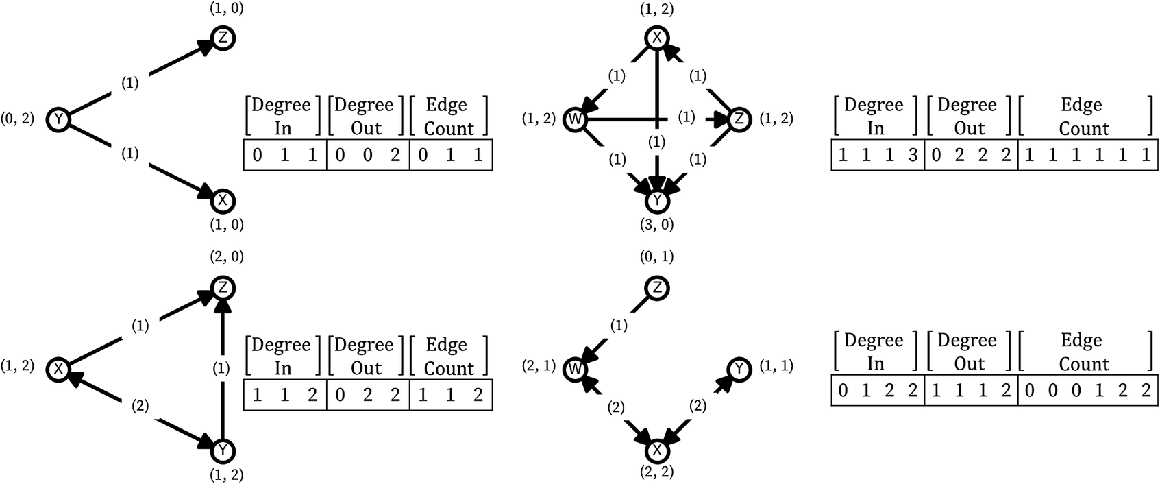
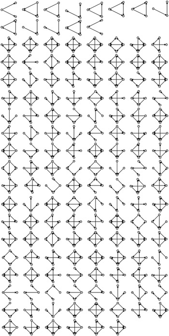
The second step is to categorize the subgraphs into unique patterns. Each subgraph belongs to a unique pattern (for example, Figure 3) that may not be directly identifiable because subgraphs can be visually oriented in different ways (also called isomorphs) and the nodes/edges can be labelled differently. To match the subgraphs into unique pattern categories, it is necessary to extract unique features and represent them using canonical forms (Chomsky Reference Chomsky1965). As shown in Figure 3, we find and sort the in- and out-degrees of nodes and the number of edges between individual node pairs. The numeric identifier stated alongside the examples shown in Figure 3 can be considered canonical forms that are identical for all isomorphs of a subgraph pattern. We find exactly 13 distinct canonical forms for 3-node subgraphs, consistent with 13 patterns in the literature (Milo et al. Reference Milo, Shen-Orr, Itzkovitz, Kashtan, Chklovskii and Alon2002, p. 824). In total, we identify 13 and 134 patternsFootnote 11 of, respectively, 3-node and 4-node subgraphs, as shown in Appendix B.
Obtaining canonical forms for 3-node and 4-node patterns to match with isomorphs.
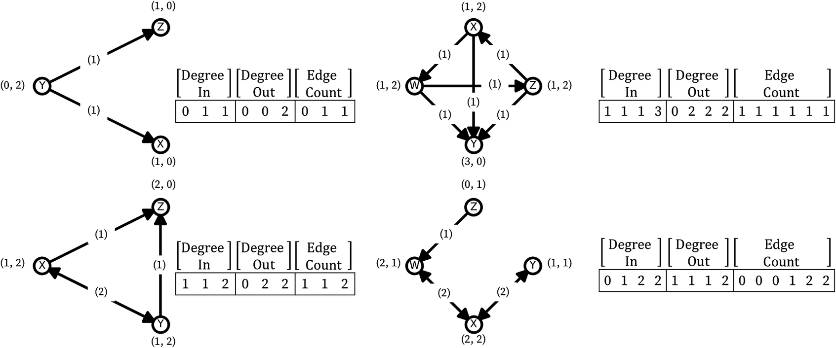
Figure 3. Long description
Panel 1, top-left, shows a directed graph with nodes Y, X, and Z. Y has out-degree 2, in-degree 0; X has in-degree 1, out-degree 0; Z has in-degree 1, out-degree 0. Edges are Y to X and Y to Z. The table lists Degree In as 0, 0, 1; Degree Out as 1, 2, 0; Edge Count as 0, 1, 1. Panel 2, bottom-left, shows a graph with X, Y, Z. X has out-degree 1, in-degree 1; Y has out-degree 1, in-degree 2; Z has out-degree 2, in-degree 1. Edges are X to Z, Y to X, Y to Z. The table lists Degree In as 1, 1, 2; Degree Out as 1, 2, 1; Edge Count as 1, 1, 2. Panel 3, top-right, shows a four-node directed graph with X, Y, Z, W. All nodes have in-degree 1, out-degree 2 or 3. Edges are X to Y, X to Z, X to W, Y to Z, Y to W, Z to W. The table lists Degree In as 1, 1, 1, 3; Degree Out as 0, 2, 2, 2; Edge Count as 1, 1, 1, 1, 1, 1. Panel 4, bottom-right, shows a four-node directed graph with X, Y, Z, W. X and Y each have in-degree 2, out-degree 2; Z and W each have in-degree 1, out-degree 1. Edges are X to Y, X to Z, Y to X, Y to W, Z to X, Z to Y, W to X, W to Y. The table lists Degree In as 0, 1, 2, 2; Degree Out as 1, 1, 2, 2; Edge Count as 0, 0, 2, 2.
2.3.3. Randomizing graphs
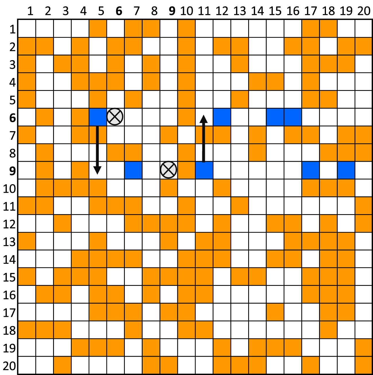
The third step is to randomize each patent knowledge graph to create a null model that could help in understanding the significance of a subgraph pattern in the original graph. Such randomization should retain some properties of the original graph. In biology literature, (Alon Reference Alon2006, p. 27) generates an ensemble of Erdos–Renyi random graphs with the same number of nodes as that of sensory–transcription networks. Watts & Strogatz (Reference Watts and Strogatz1998, pp. 440, 441) propose rewiring of edges that induce randomness, preserving the number of nodes as well as edges. In ecological networks, Stone, Simberloff, & Artzy-Randrup (Reference Stone, Simberloff and Artzy-Randrup2019, p. 4) propose dual edge swapping between edges such that the degree distribution is also retained. As edge swapping can take up to 50,000 iterations to attain a 50% perturbed random graph, Strona et al. (Reference Strona, Nappo, Boccacci, Fattorini and San-Miguel-Ayanz2014, pp. 3, 4) propose a computationally efficient “curveball” algorithm, which we adopt in our work. We prioritize computational efficiency primarily because of the sparsity of the patent knowledge graphs (mean degree = 1.839) that require several iterations to output a distinguishable randomized graph – preferably with 50% different edges. As illustrated in Figure 4, edge swapping is done between two randomly selected nodes until 50% perturbation is achieved. While swapping, we additionally include a constraint that a node cannot self-relate,Footnote 12 which was not imposed in Strona et al. (Reference Strona, Nappo, Boccacci, Fattorini and San-Miguel-Ayanz2014).
Illustrating the curveball algorithm.
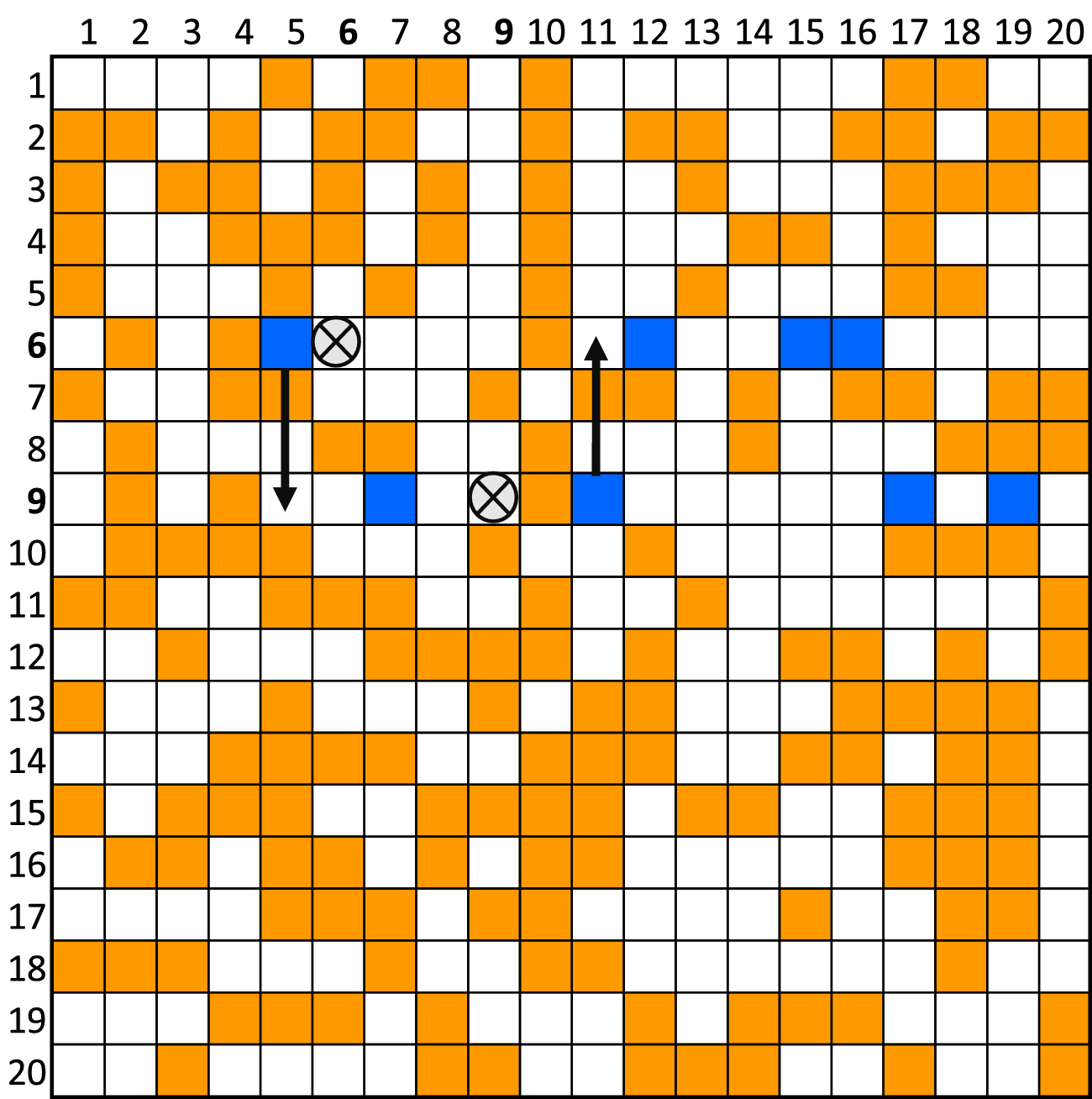
Figure 4. Long description
This is a twenty by twenty grid with columns numbered one to twenty at the top and rows numbered one to twenty on the left. Orange squares are scattered throughout, forming a non-uniform pattern. Blue squares are at six comma five, six comma eleven, nine comma eight, nine comma eleven, and nine comma seventeen. Two circled Xs mark six comma six and nine comma ten. A downward arrow connects six comma six to nine comma six, and an upward arrow connects nine comma ten to six comma ten, indicating vertical swaps between these positions. The rest of the grid is filled with alternating orange and white squares, with no other markings.
2.3.4. Analyzing differences
The final step involves analyzing the differences in the number of 3-node and 4-node subgraphs for each pattern between the original and randomized versions for all patent knowledge graphs. If a pattern occurs significantly more frequently in the original graph compared to the randomized version, the pattern can be considered a motif. For each graph representing a patent
$ i $
 , let us consider that a subgraph pattern
$ p $
, let us consider that a subgraph pattern
$ p $
 occurs
$ {X}_{ip} $
occurs
$ {X}_{ip} $
 and
$ {Y}_{ip} $
and
$ {Y}_{ip} $
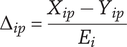
 times in the original and randomized versions, respectively. We normalize the difference between these counts using the edge count (
$ {E}_i $
times in the original and randomized versions, respectively. We normalize the difference between these counts using the edge count (
$ {E}_i $
 ) as in Equation 5 and measure the z-score of this normalized difference for all graphs in the dataset as in Equation 6, where mean (
$ {\mu}_p $
) as in Equation 5 and measure the z-score of this normalized difference for all graphs in the dataset as in Equation 6, where mean (
$ {\mu}_p $
 ) and standard deviation (
$ {\sigma}_p $
) and standard deviation (
$ {\sigma}_p $
 ) are measured across all 33,881 patent knowledge graphs.

The z-score (
$ {Z}_{ip} $
 ) as calculated in Equation 6 could tell us whether a pattern p observed in a patent graph
$ i $
) as calculated in Equation 6 could tell us whether a pattern p observed in a patent graph
$ i $
 is significantly higher than it would be by chance. At 95% confidence, we cap the z-score to 1.64 to tell whether a pattern p is a motif of the graph
$ i $
is significantly higher than it would be by chance. At 95% confidence, we cap the z-score to 1.64 to tell whether a pattern p is a motif of the graph
$ i $
 . We repeatedly perform this calculation for each 3-node and 4-node pattern (listed in Appendix B) in each patent knowledge graph.
3. Results and discussion
3.1. Linguistic foundations – entity and relationship syntaxes
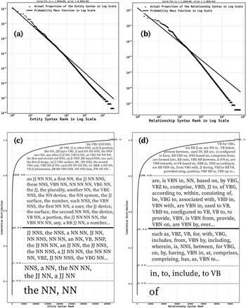
Following the methods described in Section 2.2, we transform the entities and relationships in patent knowledge graphs into unique syntaxes and rank them according to their frequencies. Upon fitting the frequency proportions of entity and relationship syntaxesFootnote 13 (Figure 5a,b) onto the probability function as in Equation 3, we discuss the syntaxes at different percentiles using the cumulative distribution as in Figure 5c,d.
Probability Zipf distribution and cumulative Zipf distribution of (5a and 5c) entity and (5b and 5d) relationship syntaxes. Syntaxes are linguistic forms expressed using frequent words and parts of speech tags like NN, VB, JJ and others.
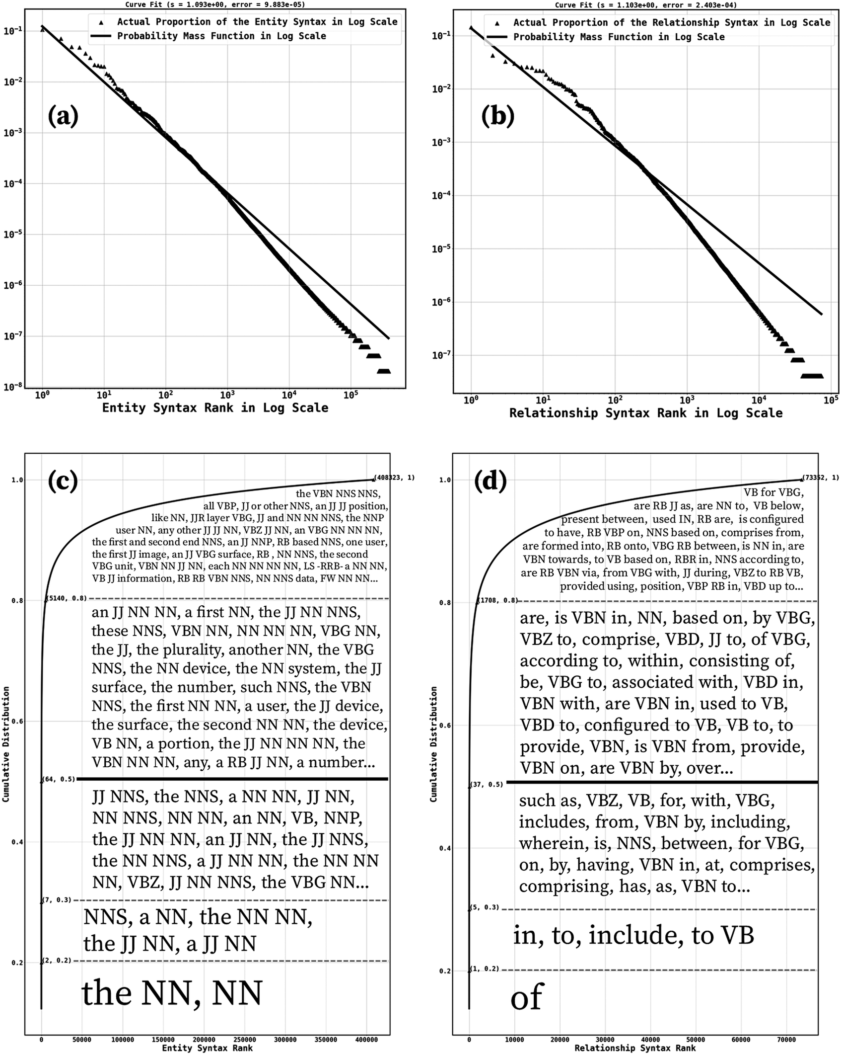
Figure 5. Long description
Panel a, top-left, is a log-log line graph with x-axis labeled Entity Syntax Rank in Log Scale and y-axis labeled Actual Proportion of the Entity Syntax in Log Scale. Two curves are shown: triangles for actual proportions and a solid line for the probability mass function. Both curves decrease steeply, showing a power-law trend. Panel b, top-right, is a similar log-log line graph with x-axis labeled Relationship Syntax Rank in Log Scale and y-axis labeled Actual Proportion of the Relationship Syntax in Log Scale. It also shows two steeply decreasing curves, with a fitted line and actual data points. Panel c, bottom-left, is a cumulative distribution plot with x-axis labeled Entity Syntax Rank and y-axis labeled Cumulative Distribution. The plot is annotated with nested text blocks, each containing frequent entity syntaxes such as ‘the N N, N N, NNS, a N N, the JJ N N,’ and others, arranged from bottom to top as rank increases. Panel d, bottom-right, is a cumulative distribution plot with x-axis labeled Relationship Syntax Rank and y-axis labeled Cumulative Distribution. It contains nested text blocks with frequent relationship syntaxes such as ‘of, in, to, include, to VB,’ and others, arranged from bottom to top as rank increases. All panels use log scales for axes except the cumulative plots, and all text is rendered exactly as shown in the plots.
In the first half of the entity syntax distribution (Figure 5c), single nouns (NN, the NN, for example, cardboard, the processor) constitute the most basic and frequent linguistic forms, which are a commonly recognized form for identifying components, processes and all constituents of an artifact in engineering design literature (Hirtz et al. Reference Hirtz, Stone, McAdams, Szykman and Wood2002; Fu et al. Reference Fu, Cagan, Kotovsky and Wood2013; Fantoni et al., Reference Fantoni, Coli, Chiarello, Apreda, Dell’Orletta and Pratelli2021). As single nouns cannot often pack a lot of information, these are extended to relatively complex forms with other nouns (proper – NNP and plural – NNS), adjectives (JJ) and verbs (VB). In the second half of the entity syntax distribution, we can observe several complex forms, which, according to Hagoort (Reference Hagoort2019), are formed by hierarchically associating basic forms, for example, “the front facing surface” = [“facing” [“front” [“surface”]]]. Hence, the most basic forms, that is, 64 syntaxes in the first half of the distribution, constitute the linguistic foundations for complex entity syntaxes and, in general, the knowledge of technological artifacts.
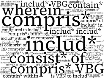
In the first half of the relationship syntax distribution (Figure 5d), “of” constitutes the most basic and frequent relationship, commonly used to capture the attribute, subsystem or subprocess of a larger entity. Besides, “in” and “to” capture various structural and behavioral relationships depending on the context. For instance, “to” can be mentioned in the transition sense, for example, “changed from… to…,” in an introductory sense, for example, “related to… and to…,” or in a utility sense, for example, “to deliver…” as expressed by the “to VB” syntax. Along with these, we observe “such as” – an exemplar relationship that is often used in instances like “volatile components such as X, Y, Z….” We then observe single verbs (“VBZ,” “VB”), which are considered to be common linguistic representatives of relationships (Jamrozik & Gentner Reference Jamrozik and Gentner2020; Siddharth et al., Reference Siddharth, Blessing, Wood and Luo2021). The hierarchical relationship “include” is the most important part of an artifact description that provides a systemic view and helps integrate and explain other constituents. To understand the hierarchical relationship further, we capture all forms of hierarchical relationships by measuring semantic similarity with “include” using Sentence TransformersFootnote 14 and display their generalizable forms in Figure 6.
Seventy-three hierarchical relationship syntaxes.
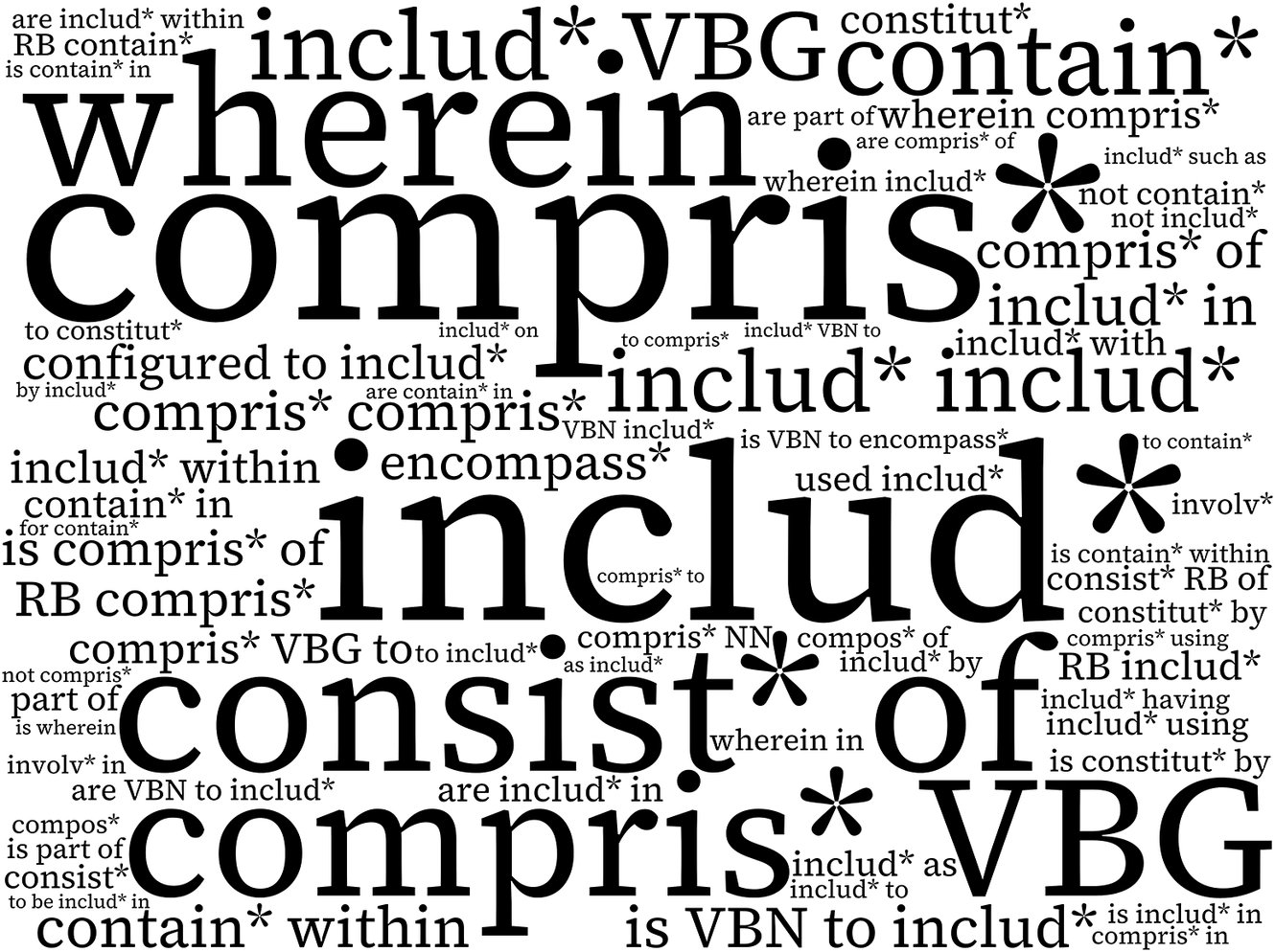
Figure 6. Long description
At the center, the largest terms are ‘wherein’, ‘compris*’, ‘includ*’, ‘consist*’, and ‘of’. Surrounding these, medium-sized terms include ‘contain*’, ‘VBG’, ‘within’, ‘configured to includ*’, ‘compos*’, ‘encompass’, ‘constitut*’, and ‘involv*’. Smaller terms radiate outward, such as ‘is compris* of’, ‘is VBN to includ*’, ‘used includ*’, ‘not contain*’, ‘part of’, ‘by includ*’, ‘as includ*’, ‘with’, ‘to contain*’, ‘is contain* within’, ‘is part of’, ‘are compris* of’, ‘compris* using’, ‘compris* NN’, ‘compris* VBG to’, ‘compris* RB of’, ‘compris* VBN to’, ‘compris* to’, ‘compris* within’, ‘compris* with’, ‘compris* in’, ‘compris* by’, ‘compris* as’, ‘compris* such as’, ‘compris* on’, ‘compris* having’, ‘compris* to includ*’, ‘compris* within’, ‘compris* to encompass’, ‘compris* by includ*’, ‘compris* to contain*’, ‘compris* to consist*’, ‘compris* to compos*’, ‘compris* to configur*’, ‘compris* to constitut*’, ‘compris* to involv*’, ‘compris* to part of’, ‘compris* to used’, ‘compris* to with’, ‘compris* to within’, ‘compris* to with’, ‘compris* to as’, ‘compris* to by’, ‘compris* to such as’, ‘compris* to on’, ‘compris* to having’, ‘compris* to to’, ‘compris* to to includ*’, ‘compris* to to encompass’, ‘compris* to to contain*’, ‘compris* to to consist*’, ‘compris* to to compos*’, ‘compris* to to configur*’, ‘compris* to to constitut*’, ‘compris* to to involv*’, ‘compris* to to part of’, ‘compris* to to used’, ‘compris* to to with’, ‘compris* to to within’, ‘compris* to to as’, ‘compris* to to by’, ‘compris* to to such as’, ‘compris* to to on’, ‘compris* to to having’. The asterisk denotes wildcard forms, and VBG, VBN, RB, NN are grammatical tags. The arrangement visually emphasizes frequency by size and centrality.
3.2. Structural foundations – motifs
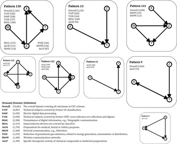
Following the methods described in Section 2.3, we identify the motifs for each patent knowledge graph in the dataset of 33,881 knowledge graphsFootnote 15. Across patents, we select the motifs that occur significantly higher than the others with 99% confidenceFootnote 16. Such motifs can be considered to constitute the structural foundations of the knowledge of technological artifacts. As shown in Figure 7, we select such motifs that are dominant overall or within the largest domainsFootnote 17 given by the CPC scheme. These motifs have also been identified in previous studies. We recall them to know whether their interpretations can help us understand the motifs that we have identified from the knowledge graphs of patent descriptions.
Dominant motifs overall and within the largest classes. For each motif pattern, we indicate the number of patents in “(.)” alongside the domain code.
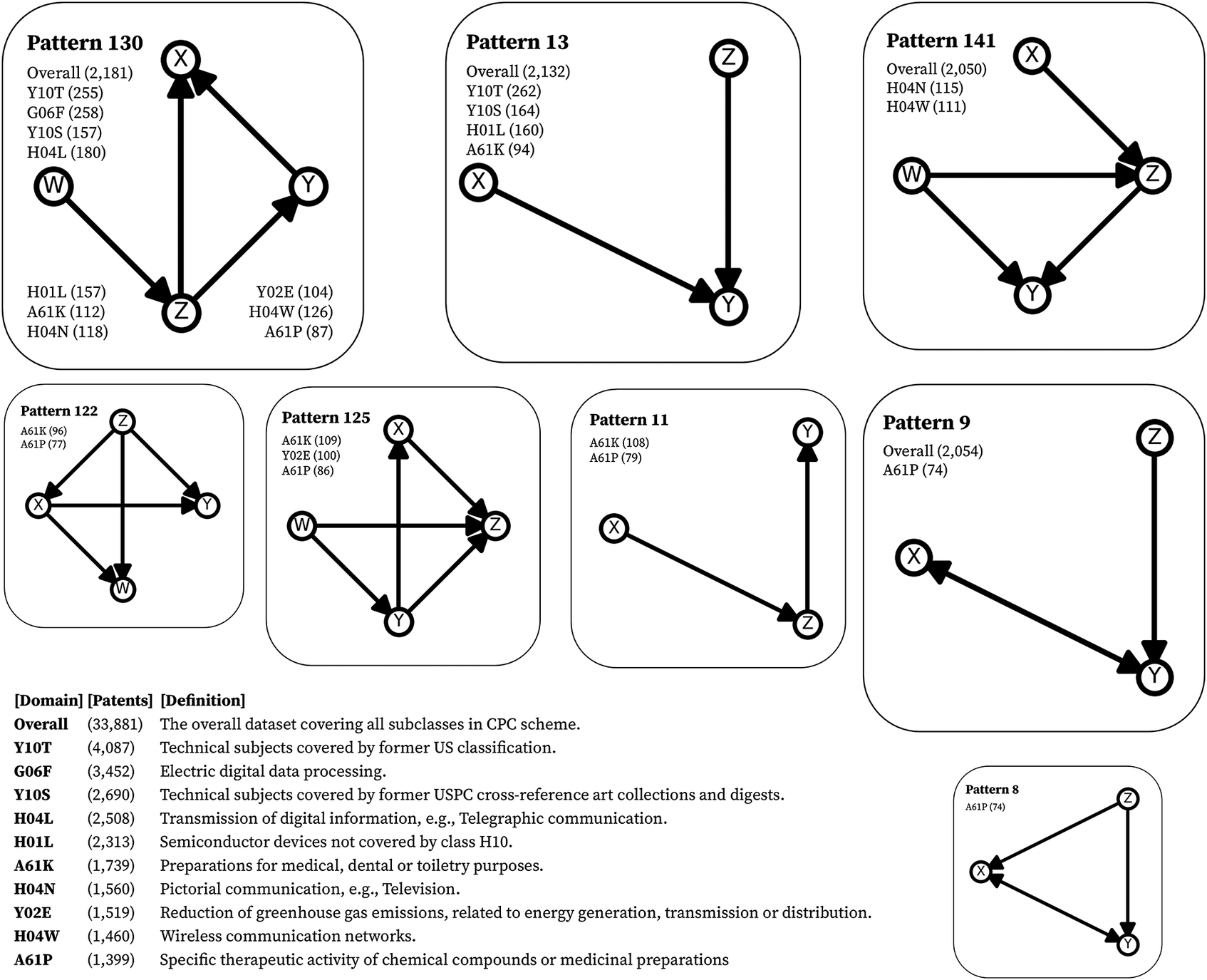
Figure 7. Long description
From the top left, Pattern 130 displays a four-node motif with arrows from W to X, X to Y, Y to Z, and Z to X. Labels: Overall 2,181, Y 1 O T 255, G 0 6 F 258, Y 1 0 S 157, H 0 4 L 180, H 0 1 L 157, A 6 1 K 112, H 0 4 N 118, Y 0 2 E 104, H 0 4 W 126, A 6 1 P 87. Next right, Pattern 13 shows a three-node motif with arrows from X to Y, Y to Z, and Z to X. Labels: Overall 2,132, Y 1 O T 262, Y 1 0 S 164, H 0 1 L 160, A 6 1 K 94. Pattern 141, top right, is a four-node motif with arrows from X to Z, W to Z, Z to Y, and Y to W. Labels: Overall 2,050, H 0 4 N 115, H 0 4 W 111. Bottom row, leftmost, Pattern 122 is a four-node motif with arrows forming a square: X to Y, Y to Z, Z to W, W to X. Labels: A 6 1 K 96, A 6 1 P 7. Pattern 125, next right, is a four-node motif with arrows from W to X, X to Y, Y to Z, Z to W. Labels: A 6 1 K 109, Y 0 2 E 100, A 6 1 P 86. Pattern 11, center, is a three-node motif with arrows from X to Y and Y to Z. Labels: A 6 1 K 108, A 6 1 P 79. Pattern 9, right, is a three-node motif with arrows from X to Y and Y to Z. Labels: Overall 2,054, A 6 1 P 74. Pattern 8, bottom right, is a three-node motif with arrows forming a triangle: X to Y, Y to Z, Z to X. Label: A 6 1 P 74. The legend below defines each domain code and provides patent counts and definitions.
In patent citation networks, Zhang, Zhang, & Wang (Reference Zhang, Zhang and Wang2024) mention the recurrence of direct citation (or sequence) and co-citation (or aggregation) as represented by Patterns 11 and 13, respectively. They note that such triangular structures induce an “echo-chamber effect” in which such structures reinforce themselves, leading to greater connectivity and lower entropy. Hence, Patterns 11 and 13 should contribute greatly to the connectivity of overall knowledge graphs of patents and thus form an imperative part of the structural foundations of the knowledge of technological artifacts. Pattern 11 is termed “sequence” in Fu et al. (Reference Fu, Cagan, Kotovsky and Wood2013, p. 5), where representative structures in patent–patent similarity networks were identified. Patterns 130 and 141 include a parallel link between two nodes that are sequentially connected. Fu et al. (Reference Fu, Cagan, Kotovsky and Wood2013, p. 5) refer to such representations as “order,” whereas Alon (Reference Alon2006, p. 45) labels them as “feed-forward loop” as found in sensory transcription networks.
Pattern 8 resembles “within-unit reciprocity,” which is found in organizational interaction networks (Brennecke et al. Reference Brennecke, Sofka, Wang and Rank2021, p. 8). Surprisingly, none of the motifs represent or extend “cyclic-closure” [↻], which is a common conceptualization scheme in various fields (Brennecke et al. Reference Brennecke, Sofka, Wang and Rank2021, p. 8), while also being identified among the patent structures in Fu et al. (Reference Fu, Cagan, Kotovsky and Wood2013, p. 5). Patterns 122 and 125 structurally resemble “bi-fan,” which is a common motif in transcription networks (Alon Reference Alon2006, p. 93). These patterns also accommodate hierarchy [
$ \leftarrow \cdot \to $
 ], which is individually not a dominant motif from our observations, despite being commonly used for visualizing nested hierarchies and process flows (Siddharth, Chakrabarti, & Ranganath Reference Siddharth, Chakrabarti and Ranganath2020) and also identified among the representative patent database structures in Fu et al. (Reference Fu, Cagan, Kotovsky and Wood2013, p. 5).
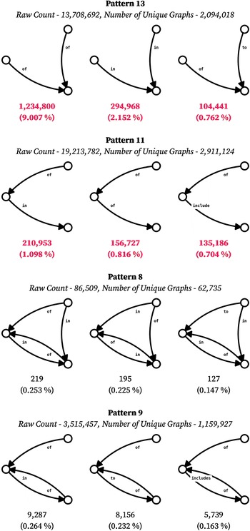
While existing studies offer unique interpretations for different motifs, their terminologies, “bi-fan,” “feed-forward loop” are specific to those networks where an edge carries a specific meaning. Such terminologies only provide limited interpretive capabilities for the motifs that we have identified from patent knowledge graphs. In Figures 8 and 9, we present the qualitative subgraphs constituting the motifs identified and showcased in Figure 7. As the motifs alone do not offer sufficient interpretive capabilities, we populate the subgraphs with edge labels falling under each subgraph pattern identified as motifs in Figures 8 and 9.
Top three most frequent subgraphs under the motifs represented by Patterns 13, 11, 8 and 9. The frequency of each subgraph and its percentage with respect to raw motif count are mentioned in the (.) beneath.
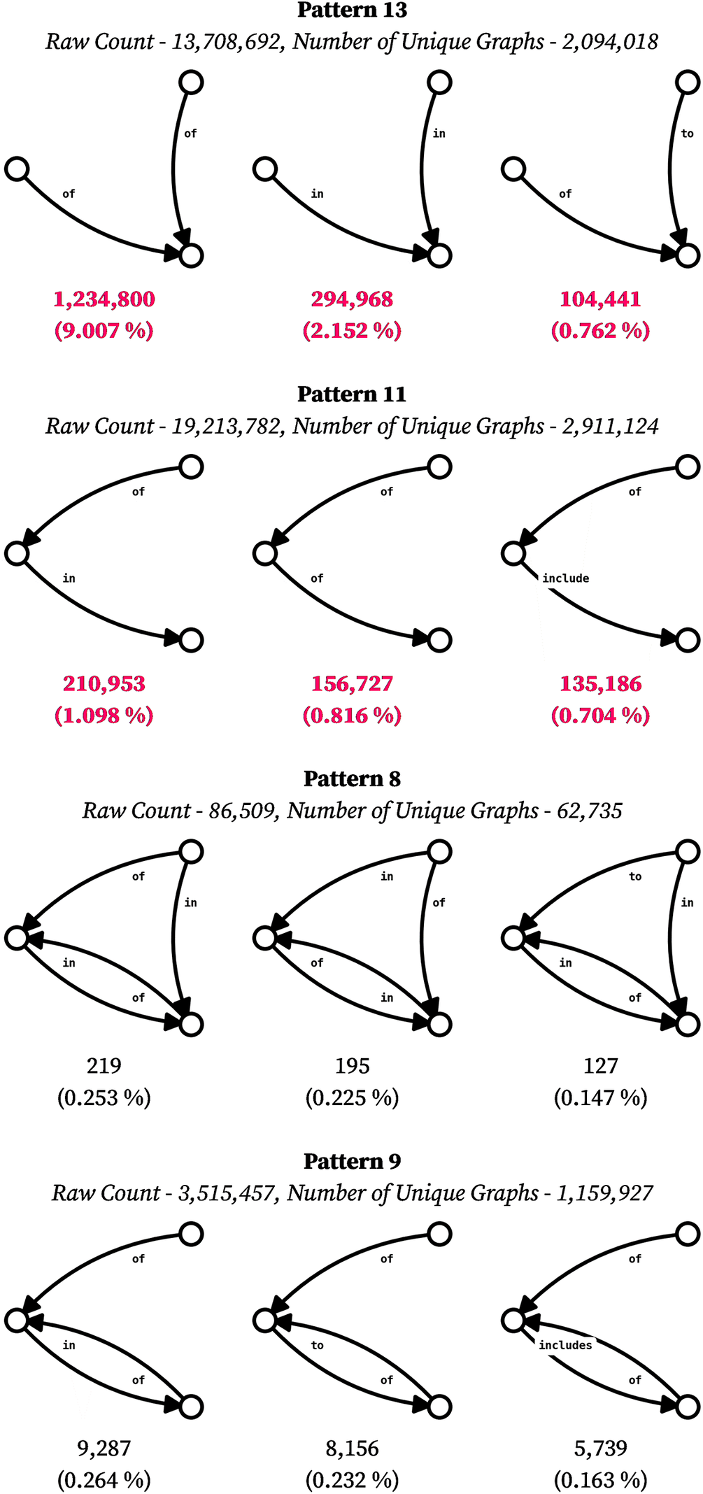
Figure 8. Long description
There are four horizontal rows, each corresponding to a motif pattern. The first row is labeled Pattern 13, with a raw count of 13,708,692 and 2,094,018 unique graphs. Three subgraphs are shown left to right: the first has arrows labeled ‘of’ and ‘in’ pointing to a filled node, with a frequency of 1,234,800 and 9.007 percent; the second has arrows labeled ‘in’ and ‘of’ converging on a filled node, frequency 294,968 and 2.152 percent; the third has arrows labeled ‘to’ and ‘of’ converging, frequency 104,441 and 0.762 percent. The second row is Pattern 11, raw count 19,213,782, unique graphs 2,911,124. The three subgraphs show: first, arrows labeled ‘of’ and ‘in’ converging, frequency 210,953 and 1.098 percent; second, arrows labeled ‘of’ and ‘in’ converging, frequency 156,727 and 0.816 percent; third, arrows labeled ‘of’ and ‘include’ converging, frequency 135,186 and 0.704 percent. The third row is Pattern 8, raw count 86,509, unique graphs 62,735. The three subgraphs show: first, arrows labeled ‘of’ and ‘in’ converging, frequency 219 and 0.253 percent; second, arrows labeled ‘of’ and ‘in’ converging, frequency 195 and 0.225 percent; third, arrows labeled ‘of’ and ‘in’ converging, frequency 127 and 0.147 percent. The fourth row is Pattern 9, raw count 3,515,457, unique graphs 1,159,927. The three subgraphs show: first, arrows labeled ‘of’ and ‘to’ converging, frequency 9,287 and 0.264 percent; second, arrows labeled ‘of’ and ‘to’ converging, frequency 8,156 and 0.232 percent; third, arrows labeled ‘of’ and ‘includes’ converging, frequency 5,739 and 0.163 percent. All frequencies and percentages are shown in pink text below each subgraph.
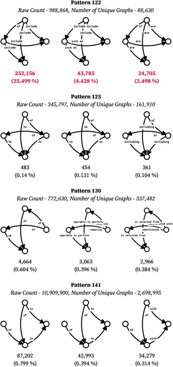
Top three most frequent subgraphs under the motifs represented by Patterns 122, 125, 130 and 141. The frequency of each subgraph and its percentage with respect to raw motif count are mentioned in the (.) beneath.
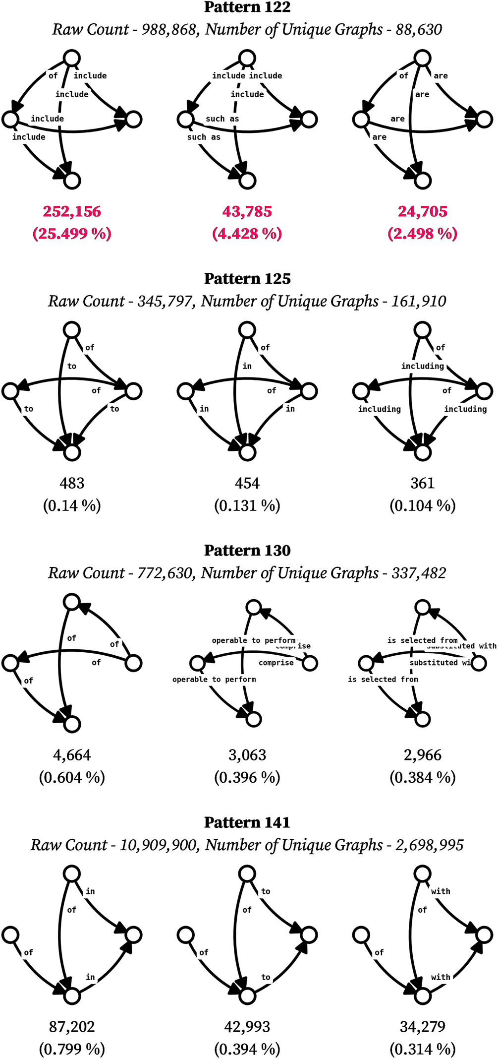
Figure 9. Long description
The diagram is divided into four horizontal sections, each labeled with a motif pattern number and its raw count and number of unique graphs. For Pattern 122, the three subgraphs (left to right) have frequencies 252,156 (25.499 percent), 43,785 (4.428 percent), and 24,705 (2.498 percent). For Pattern 125, the subgraphs have frequencies 483 (0.14 percent), 454 (0.131 percent), and 361 (0.104 percent). For Pattern 130, the subgraphs have frequencies 4,664 (0.604 percent), 3,063 (0.396 percent), and 2,966 (0.384 percent). For Pattern 141, the subgraphs have frequencies 87,202 (0.799 percent), 42,993 (0.394 percent), and 34,279 (0.341 percent). Each subgraph is a directed network with labeled edges such as include, are, in, of, to, operable to perform, comprise, selected from, substituted with, and with. The edge labels and node arrangements differ for each subgraph, visually representing the most frequent structural motifs within each pattern.
While the subgraphs in Figures 8 and 9 offer relatively better interpretation than pure motifs, we examine their frequencies to determine their generalizability. For example, the most frequent subgraph under Pattern 125 has a frequency of 483, which constitutes a minor portion (0.14%) of the raw motif count = 345,797, while the top three patterns together constitute merely 0.375% of the raw count. Such frequencies indicate that the interpretations of the qualitative subgraphs within the motifs are not sufficiently generalizable, even though the motifs (pure structure) are generalizable constituents of knowledge structures of technological artifacts. Among the patterns shown in Figures 8 and 9, we observe that the most frequent subgraphs under Patterns 122, 13 and 11 have frequencies large enough to provide relatively more generalizable interpretations compared to the remaining patternsFootnote 18. For example, the most frequent subgraph in Pattern 122 has a frequency proportion of 25.499%, while the top three subgraphs together constitute 32.426%. Hence, the interpretations made using the most frequent subgraphs under Pattern 122 could be more generalizable. Similarly, the most frequent subgraphs under Patterns 13 and 11 – in addition to pattern 122 – offer generalizable interpretations, potentially explaining the foundations of the knowledge of technological artifacts.
As observed in Figure 8, Pattern 13 uses “of” to capture multiple attributes, sub-systems or sub-processes of a higher entity in a technological artifact, for example, “temperature of the surface.” It also uses “are” to assign specific entities, for example, “the unbound candidate nucleic acids are compound A.” Pattern 11 uses “of” to capture attributes of an entity that is specified “in” another, for example, “the pressure of the liquid in state A.” Pattern 122 is a dominant motif in A61, which involves a majority of the sentences like “examples of material include compound A, compound B…” that assume hierarchical knowledge structures as in Figure 9. As Pattern 11 is a dominant motif in A61, the domain of chemical compounds for medical applications, we can observe a generalizable subgraph communicating a selection of chemical compounds, for example, “a molecule selected from the group consisting of alkyls.” Although these relationships are not common (see Figure 5d), their combination as found in Pattern 11 is more common and generalizable. Even though Patterns 13 and 11 appear to represent aggregation [
$ \to \cdot \leftarrow $
 ] and sequence [
$ \to \cdot \to $
] and sequence [
$ \to \cdot \to $
 ], most generalizable subgraphs, that reveal the actual relationships in the edge labels, tell us that these patterns capture hierarchy [
$ \leftarrow \cdot \to $
], most generalizable subgraphs, that reveal the actual relationships in the edge labels, tell us that these patterns capture hierarchy [
$ \leftarrow \cdot \to $
 ] of entities in artifacts. While Pattern 122 already exhibits a hierarchy, the most frequent subgraphs within these dominant motifs form hierarchical knowledge structures. The motifs and the underlying subgraphs showcase how knowledge is combined at a local level in technological artifact descriptions. The results shown in Figures 8 and 9 indicate that text descriptions fundamentally capture the design hierarchy of technological artifacts.
3.3. Knowledge specification strategies
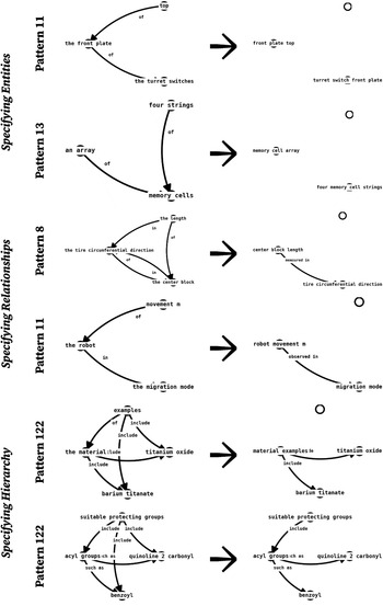
Our findings upon investigating the linguistic and structural foundations of patent documents suggest that artifact descriptions largely include abstract entities (for example, “the NN,” “JJ NNP”) that are locally connected by abstract relationships (for example, “of,” “in”) as indicated in the subgraphs of dominant motifs (Figures 8 and 9). Such abstract entities, relationships and subgraphs often constitute redundant knowledge structures. In this subsection, we showcase strategies to specify such abstract entities so that we can simplify knowledge structures derived from technological artifact descriptions. As illustrated in Figure 10, “an array and four strings of memory cells” can be captured using relatively complex entities like “memory cell array” and “four memory cell strings,” collapsing the corresponding knowledge structure, that is, Pattern 13. As most frequent relationships (“of,” “in”) lack sufficient context and thus become more mutable (Jamrozik & Gentner Reference Jamrozik and Gentner2020), they can be specified, for example, “in” ➔ “observed in” as shown in Pattern 11, Figure 10. Knowledge structures could also be simplified by eliminating redundant “include” edges, as indicated with the “acyl groups” example.
Illustrating specification of knowledge entities (Adjustable tonneau cover - https://patents.google.com/patent/US11084362B2/; Memory configured to perform logic operations on values representative of sensed characteristics of data lines and a threshold data value – https://patents.google.com/patent/US11074982/), relationships (Pneumatic tire for heavy loads – https://patents.google.com/patent/US10308079/; Autonomous mobile robot system – https://patents.google.com/patent/US9229454B1/) and hierarchical structures (Dispersion liquid, composition, film, manufacturing method of film and dispersant – https://patents.google.com/patent/US10928726/; Polar-substituted hydrocarbons – https://patents.google.com/patent/US6071895/).
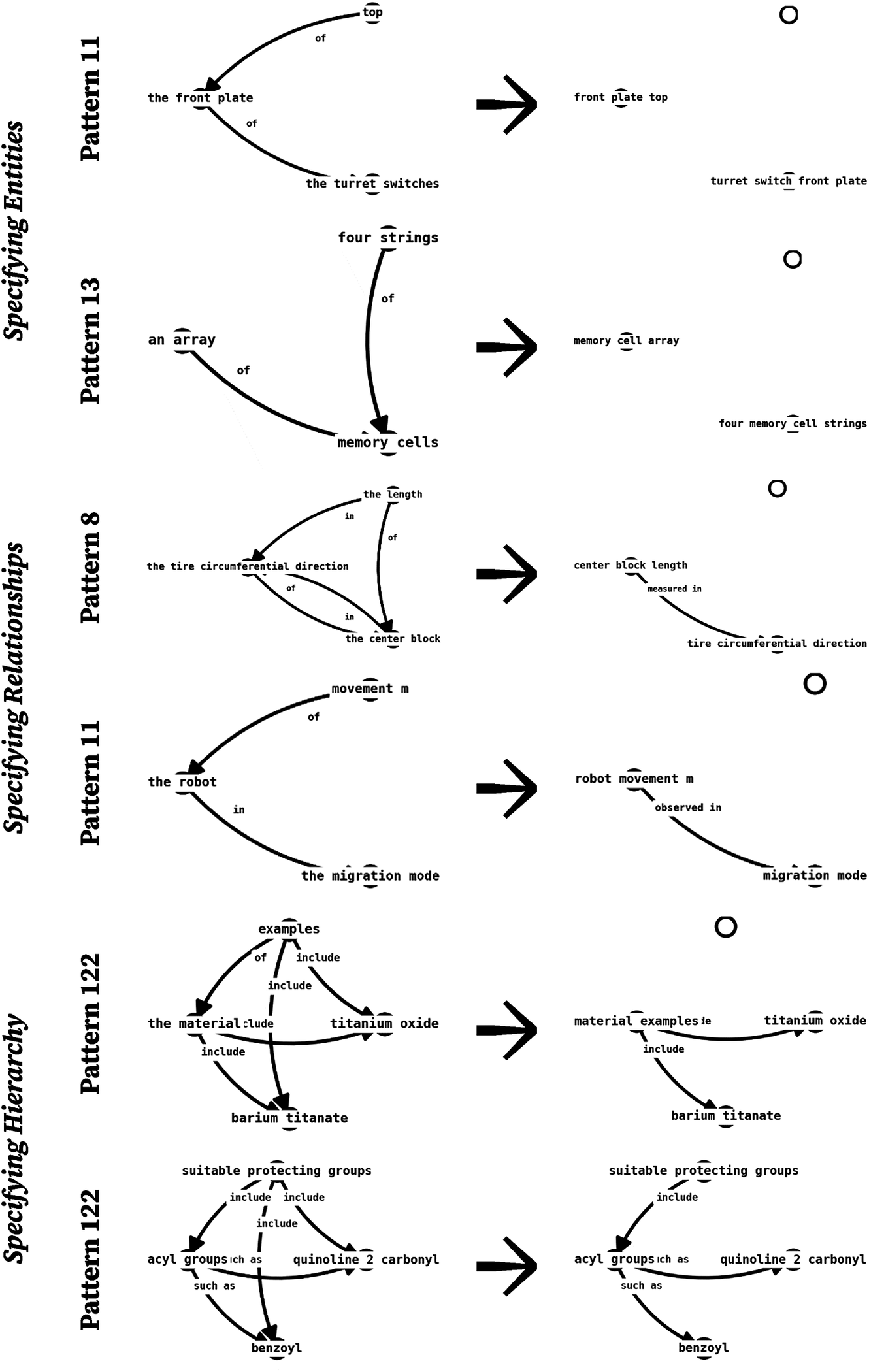
Figure 10. Long description
From top to bottom, each of the six rows illustrates a pattern for knowledge specification. The left column contains directed labeled graphs with arrows showing relationships among terms. For example, the first row (Pattern 11, Specifying Entities) shows arrows from ‘the front plate’ to ‘top’ and from ‘the turret switches’ to ‘the front plate.’ The center column translates these into a single arrow with simplified labels, such as ‘front plate top.’ The right column presents the most condensed form, e.g., ‘turret switch front plate top.’ The second row (Pattern 13) shows ‘an array of memory cells’ and ‘four strings of memory cells,’ simplified to ‘memory cell array’ and ‘four memory cell strings.’ The third and fourth rows (Pattern 8 and Pattern 11, Specifying Relationships) show relationships like ‘the tire circumferential direction in the center block’ and ‘the robot movement in the migration mode,’ each simplified in the center and right columns. The last two rows (Pattern 122, Specifying Hierarchy) show hierarchical inclusion, such as ‘the material includes titanium oxide and barium titanate,’ and ‘suitable protecting groups include acyl groups such as quinoline 2 carbonyl and benzoyl,’ with arrows indicating inclusion and examples. Each pattern demonstrates the transformation from detailed relational graphs to concise text representations, emphasizing structural and hierarchical relationships.
The examples shown in Figure 10 indicate a broad limitation of using natural language in technological artifact descriptions. The example of Pattern 11 in Figure 10 is derived from the text, “movement m of the robot in the migration mode,” which shows that “movement m” and “the robot” are mentioned abstractly to associate them with other entities of the overall patent artifact – for example, “the path and duration of movement m are better than movement n of the robot.” In this sentence, knowledge is not captured individually through entities such as “path,” “duration,” “movement” and “robot,” but through their verbal and syntactical associations in the sentence. In order to densely pack information within a sentence, it is necessary to keep the entities as simple as possible while introducing several connections among them. As a consequence, we observe that the majority of the entities are abstract nouns (Figure 5) that are associated using abstract relationships (Figures 8 and 9).
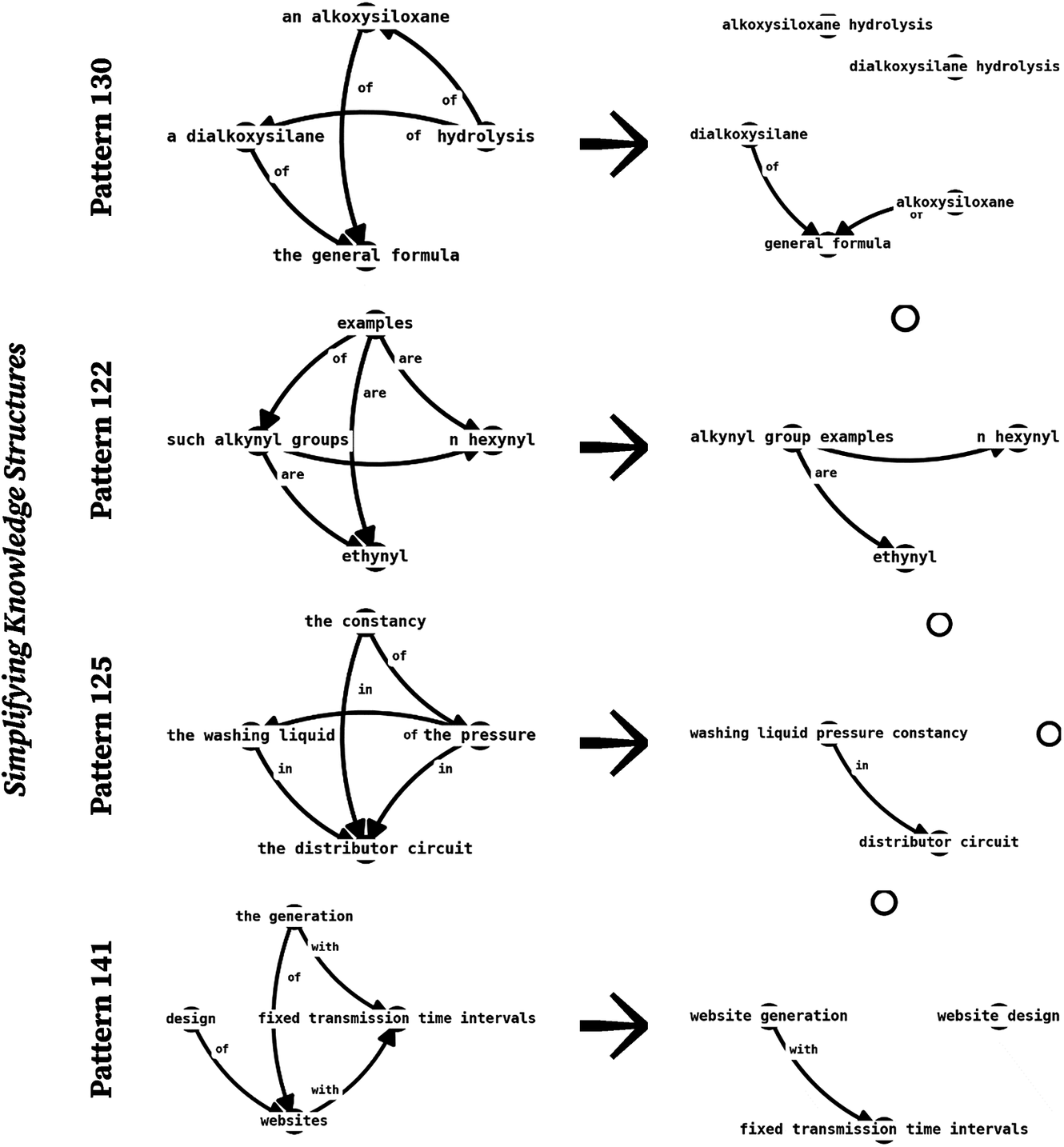
The sentence can alternatively be written as, “the robot movement m path and the robot movement m duration are better than the robot movement n path and the robot movement n duration.” It is, however, impractical to have artifact knowledge documented in this manner. Alternatively, we can re-represent the knowledge extracted from natural language text, however it is written, so that knowledge constituents such as entities and relationships in the knowledge graphs are less abstract and thus more specific. As illustrated further in Figure 11, the specification strategies can also help modularize the structure of patent knowledge graphs. Effectively modularizing systems can incur various benefits, such as change management, intellectual property protection, technical robustness and others (Baldwin & Henkel Reference Baldwin and Henkel2015; Siddharth & Sarkar Reference Siddharth and Sarkar2018, Reference Siddharth and Sarkar2017). In the patent literature, Siddharth (Reference Siddharth2025) observes that modularizing knowledge structures enhances the technological impact of patents.
Illustrating simplification of knowledge structures using examples of Pattern 130 (Process for preparing low molecular weight organosiloxane terminated with silanol group – https://patents.google.com/patent/US5576408/), 122 (Polar-substituted hydrocarbons – https://patents.google.com/patent/US6071895/), 125 (Machine for washing objects and method for the hydraulic and mechanical connection of a trolley carrying objects to be washed to a feed circuit of a washing liquid for a machine for washing objects – https://patents.google.com/patent/US9393600/) and 141 (Systems and methods for loading websites with multiple items – https://patents.google.com/patent/US11055378/).
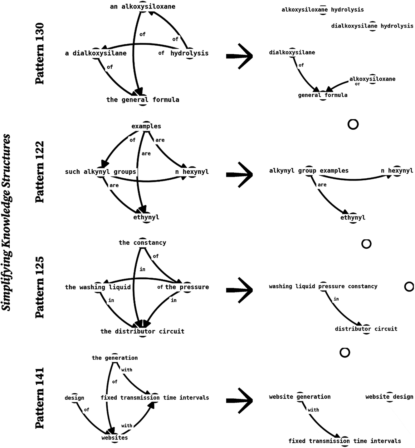
Figure 11. Long description
From top to bottom, each row contains two directed network diagrams separated by a rightward arrow. The left diagram in each row is a dense network of labeled nodes and arrows, while the right diagram is a more linear or reduced version. Row one (Pattern 130) starts with nodes labeled ‘an alkoxysiloxane’, ‘a dialkoxysilane’, ‘hydrolysis’, and ‘the general formula’, connected by arrows labeled ‘of’, leading to a simplified network with ‘dialkoxysilane’ and ‘alkoxysiloxane hydrolysis’ linked to ‘general formula’. Row two (Pattern 122) begins with nodes ‘such alkynyl groups’, ‘examples’, ‘n hexynyl’, and ‘ethynyl’, with arrows labeled ‘are’ and ‘of’, simplified to ‘alkynyl group examples’ leading to ‘n hexynyl’ and ‘ethynyl’. Row three (Pattern 125) has nodes ‘the washing liquid’, ‘the constancy’, ‘of the pressure’, and ‘the distributor circuit’, with arrows labeled ‘of’ and ‘in’, simplified to ‘washing liquid pressure constancy’ leading to ‘distributor circuit’. Row four (Pattern 141) starts with ‘the generation’, ‘design’, ‘fixed transmission time intervals’, and ‘websites’, with arrows labeled ‘of’ and ‘with’, simplified to ‘website generation’ and ‘website design’ leading to ‘fixed transmission time intervals’. Each simplified network is more linear, with fewer nodes and connections than its corresponding complex version.
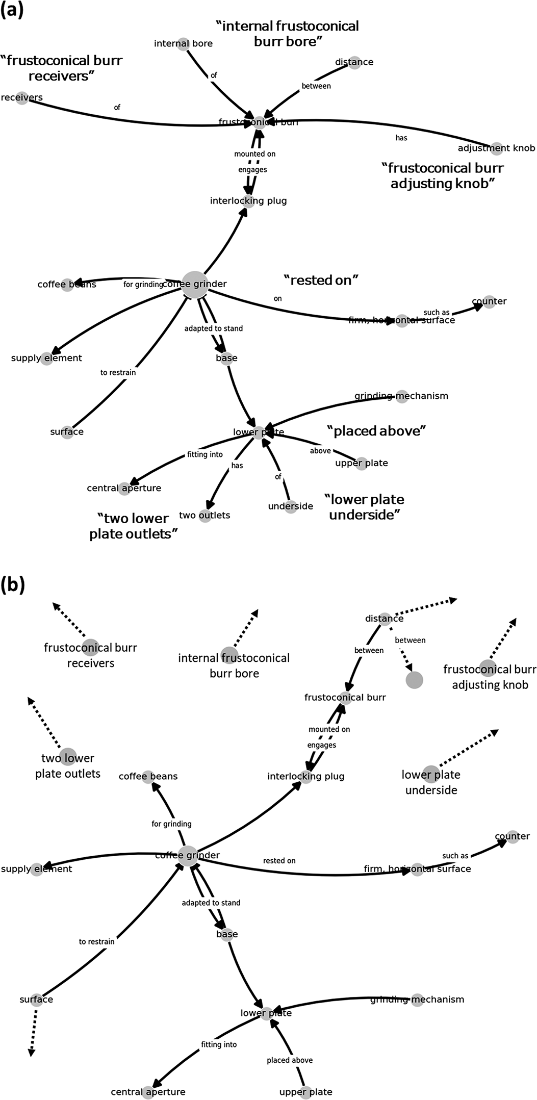
We apply the knowledge specification strategies to the domain of coffee grinder patents, as shown in Figure 12. For this purpose, we retrieved the full text of seven patents having the title “coffee-grinder.” We apply our knowledge graph extraction method (Siddharth & Luo Reference Siddharth and Luo2024; Siddharth Reference Siddharth2024a) to the descriptions of these coffee-grinder patents to extract 3,618 facts. Among these, we filter 320 generalizable facts that have a frequency
$ \ge $
 2. In Figure 12-a, we combine the facts around the core entity – “coffee grinder” and visualize them as a knowledge graph. In this knowledge graph, the unlabeled edges indicate a hierarchical relationship – most commonly represented by “include” and alternatively using other forms as indicated in Figure 6. The labelled edges mention a specific relationship between a pair of entities. Hence, both hierarchical and other relationships represent associations among common entities surrounding a coffee grinder. This knowledge graph serves as an explicit representation of generalizable domain knowledge of coffee grinders, as derived from the corresponding patent descriptions.
(a) Extended neighborhood of “coffee grinder” entity. The edges without a label indicate a hierarchical relationship – “include.” (b) Transformed extended neighborhood of “coffee grinder” entity. The edges without a label indicate a hierarchical relationship – “include.”
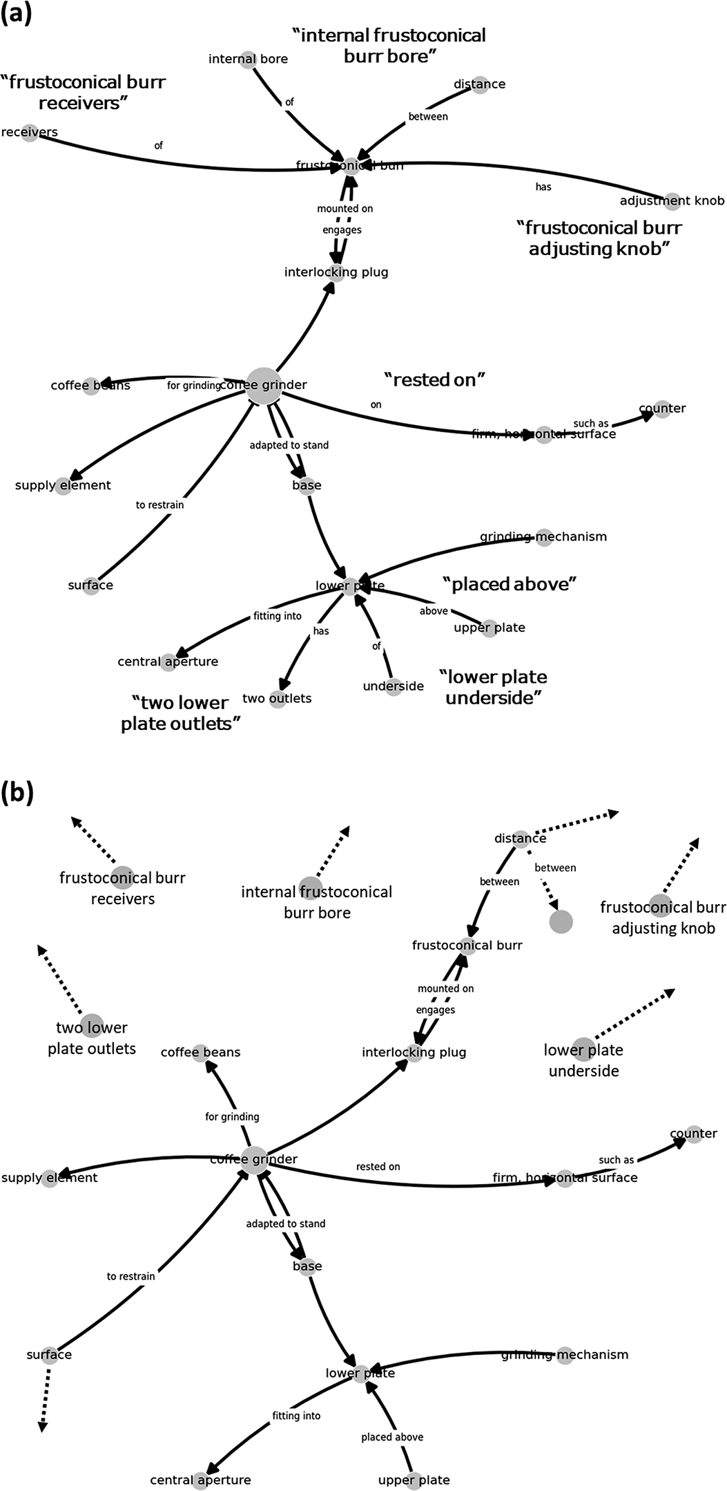
Figure 12. Long description
Panel one, at left, centers on a gray node labeled coffee grinder. Outward branches connect to coffee beans, supply element, surface, frustoconical burr, interlocking plug, base, and lower plate. The frustoconical burr node branches to frustoconical burr receivers, internal frustoconical burr bore, and frustoconical burr adjusting knob. Internal frustoconical burr bore connects to internal bore and distance between. Frustoconical burr adjusting knob connects to adjustment knob. Lower plate branches to central aperture, two lower plate outlets, lower plate underside, and upper plate. Labeled edges specify relationships such as for grinding, mounted on, engages, adapted to stand, fitting into, has, of, above, and on. The lower plate underside connects to grinding mechanism. The base connects to rested on, which leads to firm, horizontal surface, and counter. Unlabeled edges indicate hierarchical includes relationships. Panel two, at right, is a transformed version with similar nodes and relationships, but the structure is visually rearranged for clarity.
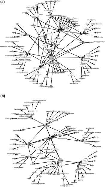
As we apply the specification strategies, we modify the fact “receivers of frustonical burr” to “frustonical burr receivers,” reducing the level of abstraction in either of the entities “receivers” and “frustonical burr.” Similarly, we specify the other entities that are associated with the “of” relationship. In addition, we specify the abstract relationships such as “coffee grinder on firm, horizontal surface” to “coffee grinder rested on firm, horizontal surface” based on the context offered by the pair of entities. Upon performing these modifications, as shown in Figure 12b, we find that the structure of the knowledge graph is more simplified and the individual entities/relationships are more enriched in terms of information content. In addition to this case study, we apply these knowledge specification strategies to a relatively more complex glue gun knowledge graph as shown in Appendix C.
4. Conclusions
In this study, we addressed the question “What is the basis of the knowledge of technological artifacts?” from a perspective different from the literature, where similar questions are often addressed through expert-defined ontologies. Drawing on 33,881 utility patent descriptions represented as knowledge graphs, we derived the foundations of artifact knowledge as generalizable linguistic syntaxes and structural motifs. The linguistic syntaxes primarily comprise noun-based entities, abstract relational terms such as “of,” “in,” and hierarchical variants of “include.” These linguistic syntaxes – derived from a large, stratified sample of patents – could be considered the primary linguistic foundations for all terms in the technology space.
Through the motif discovery approaches inspired by studies in biology and ecology, we identified eight unique subgraph patterns that represent how terms are locally combined in technological artifact descriptions. Among these, we converged on Patterns 11, 13 and 122, whose subgraphs offered generalizable interpretations based on their relatively higher frequency proportions. Examining the subgraphs within the selected patterns revealed that artifact descriptions primarily capture the design hierarchy of artifacts, largely through abstract relationships such as “of,” “in,” “include” and others. These findings could echo throughout the technology space, as we have derived them from a large, stratified sample of patents from the total technology space.
The major conclusions of this study are as follows:
-
• The knowledge of technological artifacts has simple and abstract linguistic foundations, represented by basic forms of nouns, prepositions (“of,” “in”) and verbs (“include”), which themselves combine to express complex terms and phrases.
-
• The knowledge of technological artifacts has non-random and statistically significant structural foundations, represented by a finite number of 3-node and 4-node subgraph patterns, which predominantly capture the design hierarchy of artifacts.
-
• The knowledge of technological artifacts from patent or similar natural language descriptions largely comprises abstract knowledge at the local level, where (automated) specification strategies are required for knowledge retrieval applications.
The methods and findings in this study make contributions to design literature and can enable applications in design research and practice, such as knowledge engineering, ontology extraction, function modelling, graph-based reasoning, patent search, text-mining, technology mapping and LLM-centric applications. The emphasis of findings on design hierarchy and the level of abstraction can provide an informed perspective for future design studies that leverage natural language artifact descriptions. Knowledge search is quite expensive in design and innovation processes, because of the false positives incurred by the abstract terms in natural language text sources (Han, Zhang, & Tong Reference Han, Zhang and Tong2024). Re-representing the knowledge of technological artifacts – supposedly using our specification strategies – could thus circumvent the common issues of knowledge retrieval, enhance the performance and enable trustworthy adoption of LLMs that are being increasingly utilized for knowledge retrieval (Siddharth & Luo Reference Siddharth and Luo2025).
The limitations of this study pave the way for future research directions. Currently restricted to patents from the USPTO, the study shall explore other important sources of artifact knowledge, such as scientific articles, design reports and more. The findings based on Zipf distribution analyses and motif discovery require tests of robustness, which typically involve replication of findings when patents are studied across domains, time frames, geographies and other variants. Our study must move from sample to population-level analyses to carry out such robustness checks. The proposed knowledge specification strategies are manually demonstrated with a few patents on coffee grinders and glue guns. A comprehensive demonstration with a family of products and services needs to be carried out – preferably by automating specification strategies using LLMs – and studies must be conducted to assess how they aid in knowledge representation and retrieval in the design and innovation processes.
Appendix A
List of parts-of-speech tags
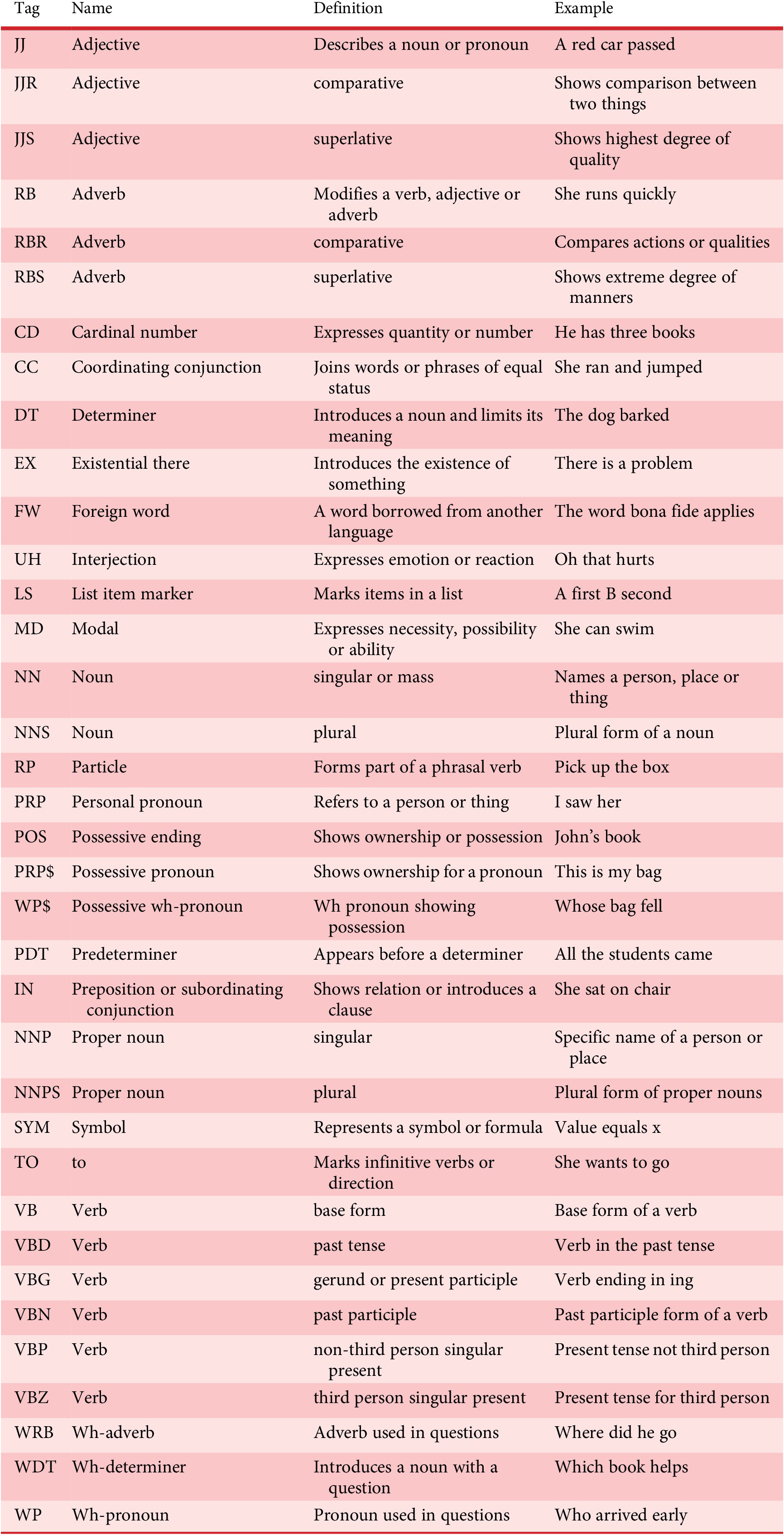
Table A1. Long description
The table begins with column headers: Tag, Name, Definition, Example. Each subsequent row presents a tag and its corresponding information. JJ is Adjective, describes a noun or pronoun, example A red car passed. JJR is Adjective comparative, shows comparison between two things. JJS is Adjective superlative, shows highest degree of quality. RB is Adverb, modifies a verb, adjective or adverb, example She runs quickly. RBR is Adverb comparative, compares actions or qualities. RBS is Adverb superlative, shows extreme degree of manners. CD is Cardinal number, expresses quantity or number, example He has three books. CC is Coordinating conjunction, joins words or phrases of equal status, example She ran and jumped. DT is Determiner, introduces a noun and limits its meaning, example The dog barked. EX is Existential there, introduces the existence of something, example There is a problem. FW is Foreign word, a word borrowed from another language, example The word bona fide applies. UH is Interjection, expresses emotion or reaction, example Oh that hurts. LS is List item marker, marks items in a list, example A first B second. MD is Modal, expresses necessity, possibility or ability, example She can swim. NN is Noun singular or mass, names a person, place or thing. NNS is Noun plural, plural form of a noun. RP is Particle, forms part of a phrasal verb, example Pick up the box. PRP is Personal pronoun, refers to a person or thing, example I saw her. POS is Possessive ending, shows ownership or possession, example John’s book. PRP dollar is Possessive pronoun, shows ownership for a pronoun, example This is my bag. WP dollar is Possessive wh-pronoun, wh pronoun showing possession, example Whose bag fell. PDT is Predeterminer, appears before a determiner, example All the students came. IN is Preposition or subordinating conjunction, shows relation or introduces a clause, example She sat on chair. NNP is Proper noun singular, specific name of a person or place. NNPS is Proper noun plural, plural form of proper nouns. SYM is Symbol, represents a symbol or formula, example Value equals x. TO is to, marks infinitive verbs or direction, example She wants to go. VB is Verb base form, base form of a verb. VBD is Verb past tense, verb in the past tense. VBG is Verb gerund or present participle, verb ending in ing. VBN is Verb past participle, past participle form of a verb. VBP is Verb non-third person singular present, present tense not third person. VBZ is Verb third person singular present, present tense for third person. WRB is Wh-adverb, adverb used in questions, example Where did he go. WDT is Wh-determiner, introduces a noun with a question, example Which book helps. WP is Wh-pronoun, pronoun used in questions, example Who arrived early. The tags and names are sourced from the Penn Tree Bank POS tag list, with a reference link provided at the bottom.
Appendix B
All 3-node and 4-node subgraph patterns.
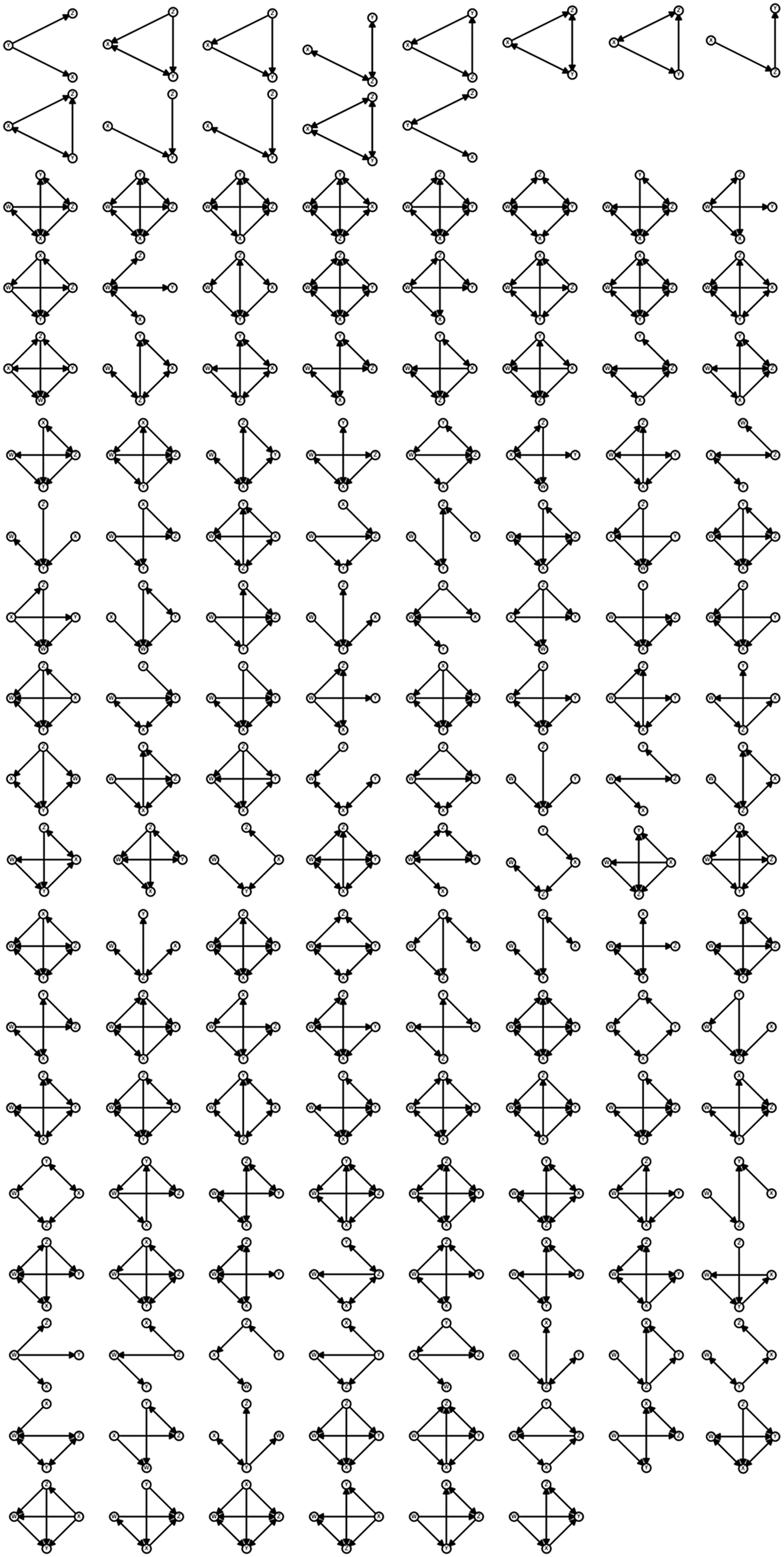
Figure B1. Long description
Starting at the top-left, the first row contains all unique directed graphs with three nodes, each represented by circles connected by arrows in every possible configuration, including isolated nodes, single edges, bidirectional edges, and cycles. From the second row onward, each cell contains a four-node directed graph, systematically varying the direction and presence of edges. The grid continues downward and rightward, with each subsequent cell representing a different arrangement, including all combinations of directed edges, cycles, and disconnected nodes. No two graphs are identical. The arrangement exhaustively enumerates all possible directed subgraph motifs for three and four nodes, with each motif visually distinct by its edge pattern.
Appendix C
(a) Extended neighborhood of “glue gun” entity. The edges without a label indicate a hierarchical relationship – “include.” (b) Transformed extended neighborhood of glue gun. The edges without a label indicate a hierarchical relationship – “include.”
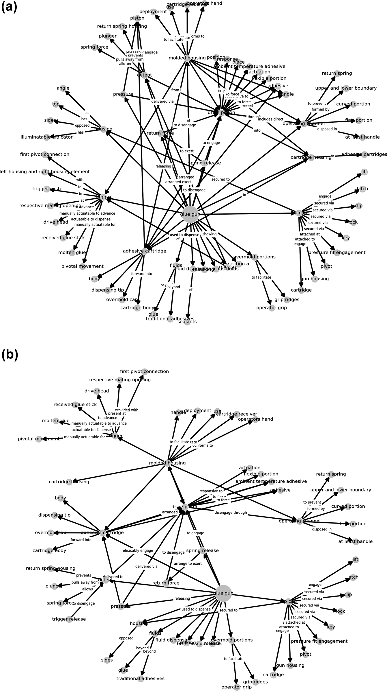
Figure C1. Long description
There are two panels arranged side by side. In the left panel, the central node labeled glue gun is surrounded by nodes such as adhesive cartridge, molded housing position, operating channel, and trigger, each connected by arrows. Labeled edges specify relationships like used to dispense, includes direct, and disposed in, while unlabeled edges indicate hierarchical inclusion. Peripheral nodes include operator’s hand, cartridge, fluids, dispensing tip, and pressure fit engagement, each branching from intermediate nodes. The right panel shows a transformed version with similar nodes and connections, but the structure is altered, redistributing nodes like molded housing position and adhesive cartridge, and reorienting the hierarchical and labeled relationships. All text labels are preserved exactly as in the diagram, with arrows indicating directionality of relationships.

 Open access

