




Introduction
Throughout the Pleistocene, there have been interglacial periods of exceptional warmth known as “super-interglacials” (Melles et al., Reference Melles, Brigham-Grette, Minyuk, Nowaczyk, Wennrich, DeConto and Anderson2012). Marine Isotope Stage (MIS) 11 (424–374 ka) is one such period, and has, in fact, been recognized as the longest (and potentially the warmest) interglacial of the past 500 ka (Hodell et al., Reference Hodell, Charles and Ninnemann2000; Berger and Loutre, Reference Berger and Loutre2002; Lisiecki and Raymo, Reference Lisiecki and Raymo2005; Rohling et al., Reference Rohling, Braun, Grant, Kucera, Roberts, Siddall and Trommer2010; PAGES Past Interglacials Working Group, Reference Berger, Crucifix, Hodell, Mangili, McManus, Otto-Bliesner and Pol2016). In addition, it is the most recent interglacial period when orbital parameters were similar to today: eccentricity was low, obliquity was high, and the amplitude of precessional changes was dampened (Berger and Loutre, Reference Berger and Loutre2002; Droxler et al., Reference Droxler, Alley, Howard, Poore, Burckle, Droxler, Poore and Burckle2003a; Loutre and Berger, Reference Loutre and Berger2003). Relatively high atmospheric CO2 concentrations of 275 ppm (Petit et al., Reference Petit, Jouzel, Raynaud, Barkov, Barnola, Basile and Bender1999; Siegenthaler et al., Reference Siegenthaler, Stocker, Monnin, Lüthi, Schwander, Stauffer and Raynaud2005; Lüthi et al., Reference Lüthi, le Floch, Bereiter, Blunier, Barnola, Siegenthaler and Raynaud2008; Bereiter et al., Reference Bereiter, Eggleston, Schmitt, Nehrbass-Ahles, Stocker, Fischer, Kipfstuhl and Chappellaz2015) contributed to the extreme warmth recorded in the proxy record; MIS 11 would otherwise have been much cooler, due to low insolation values throughout (Yin and Berger, Reference Yin and Berger2011). The interglacial climatic optimum (MIS 11c) lasted on the order of 10–30 ka and was characterized by higher than present sea level (Raymo and Mitrovica, Reference Raymo and Mitrovica2012; Dutton et al., Reference Dutton, Carlson, Long, Milne, Clark, DeConto, Horton, Rahmstorf and Raymo2015), enhanced calcareous plankton blooms at high latitudes, and the expansion of coral reefs (Droxler and Farrell, Reference Droxler and Farrell2000). During MIS 11c, Antarctic temperatures were up to 2°C warmer than today (Jouzel et al., Reference Jouzel, Masson-Delmotte, Cattani, Dreyfus, Falourd, Hoffmann and Minster2007), boreal forest extended across southern Greenland (de Vernal and Hillaire-Marcel, Reference de Vernal and Hillaire-Marcel2008; Kleinen et al., Reference Kleinen, Hildebrandt, Prange, Rachmayani, Mueller, Bezrukova, Brovkin and Tarasov2014), northwestern Greenland was ice free (Christ et al., Reference Christ, Rittenour, Bierman, Keisling, Knutz, Thomsen and Keulen2023), and large lakes in Siberia were anomalously productive (Prokopenko et al., Reference Prokopenko, Bezrukova, Khursevich, Solotchina, Kuzmin and Tarasov2010; Lozhkin and Anderson, Reference Lozhkin and Anderson2013), with warmer than present summer air temperatures (Melles et al., Reference Melles, Brigham-Grette, Minyuk, Nowaczyk, Wennrich, DeConto and Anderson2012). In addition, there is evidence that sea-surface temperature (SST) was elevated and summer sea ice was absent from the Arctic Ocean for much of MIS 11 (Cronin et al., Reference Cronin, Polyak, Reed, Kandiano, Marzen and Council2013, Reference Cronin, Keller, Farmer, Schaller, O’Regan, Poirier, Coxall and Dwyer2019; Hu et al., Reference Hu, Marino, Pérez-Mejías, Spötl, Yokoyama, Yu and Rohling2024).
Despite the work done to characterize the warmth of MIS 11 on land (e.g., Droxler et al., Reference Droxler, Poore and Burckle2003b; Ashton et al., Reference Ashton, Lewis, Parfitt, Penkman and Coope2008; Candy, Reference Candy2009; Candy et al., Reference Candy, Schreve, Sherriff and Tye2014; Kleinen et al., Reference Kleinen, Hildebrandt, Prange, Rachmayani, Mueller, Bezrukova, Brovkin and Tarasov2014; Tye et al., Reference Tye, Sherri, Candy, Coxon, Palmer, McClymont and Schreve2016), as well as in the North Atlantic (e.g., Kandiano and Bauch, Reference Kandiano and Bauch2007; Dickson et al., Reference Dickson, Beer, Dempsey, Maslin, Bendle, McClymont and Pancost2009; Poli et al., Reference Poli, Meyers and Thunell2010; Voelker et al., Reference Voelker, Rodrigues, Billups, Oppo, McManus, Stein, Hefter and Grimalt2010; Kandiano et al., Reference Kandiano, Bauch, Fahl, Helmke, Roehl, Perez-Folgado and Cacho2012, Reference Kandiano, van der Meer, Schouten, Fahl, Damste and Bauch2017; Milker et al., Reference Milker, Rachmayani, Weinkauf, Prange, Raitzsch, Schulz and Kucera2013), less is known about this interval from the North Pacific region. This paper is one of the first studies to produce sub-millennial-scale resolution records that elucidate the relationship between diatom productivity and sea ice extent in the Bering Sea during MIS 11. Here, we use a multiproxy approach that includes sediment grain-size measurements, diatom assemblage counts, and stable isotope analyses at Integrated Ocean Drilling Program (IODP) Site U1339 (Umnak Plateau, Bering Sea).
Study area
Located between Russia and Alaska, the Bering Sea is the northernmost marginal sea of the Pacific Ocean and the third largest marginal sea in the world. It is separated from the North Pacific by the Aleutian Islands (Fig. 1), but water mass exchange occurs through passes in the Aleutian Islands, linking Bering Sea conditions to those of the Pacific (Stabeno et al., Reference Stabeno, Schumacher, Ohtani, Loughlin and Ohtani1999). Warmer, nutrient-rich surface currents, derived from inflow of the Alaskan Stream, an extension of the Alaska Current (Fig. 1), fuel the highly productive Bering Sea ecosystem (Stabeno et al., Reference Stabeno, Danielson, Kachel, Kachel and Mordy2016). As the sole gateway between the Bering Sea and the Arctic Ocean, inflow of Pacific water through the Bering Strait (Fig. 1) is an important source of heat, relatively fresh water, and nutrients to the Arctic (Walsh et al., Reference Walsh, McRoy, Blackburn, Coachman, Goering, Henriksen, Andersen, Rey and Alexander1989; Stabeno et al., Reference Stabeno, Schumacher, Ohtani, Loughlin and Ohtani1999; Grebmeier et al., Reference Grebmeier, Overland, Moore, Farley, Carmack, Cooper, Frey, Helle, McLaughlin and McNutt2006; Woodgate et al., Reference Woodgate, Weingartner and Lindsay2010). Closure of the Bering Strait during glacial lowstands isolates the North Pacific from the North Atlantic, causing major changes in global ocean circulation, salinity, and nutrient distributions (e.g., Okazaki et al., Reference Okazaki, Timmermann, Menviel, Harada, Abe-Ouchi, Chikamoto, Mouchet and Asahi2010; Hu et al., Reference Hu, Meehl, Han, Abe-Ouchi, Morrill, Okazaki and Chikamoto2012, Reference Hu, Meehl, Han, Otto-Bliesner, Abe-Ouchi and Rosenbloom2015; Knudson and Ravelo, Reference Knudson and Ravelo2015; Caissie et al., Reference Caissie, Brigham-Grette, Cook and Colmenero-Hidalgo2016).
Map of Beringia, showing the position of Integrated Ocean Drilling Program (IODP) Site U1339 (green star), and other sites referred to in the text. The dashed line shows the maximum extent of sea ice today (median over the period 1979–2013; concentration >15%) (Cavalieri et al., Reference Cavalieri, Parkinson, Gloersen and Zwally1996). Currents (shown in blue) are modified from Stabeno et al. (Reference Stabeno, Schumacher, Ohtani, Loughlin and Ohtani1999). Abbreviations: ACC, Alaska Coastal Current; ANSC, Aleutian North Slope Current; BS, Bering Strait; BSC, Bering Slope Current; UkP, Unimak Pass; and UP, Umnak Plateau. Gray bathymetric shading changes value at −50 m (Bering Strait sill depth), −250 m (shelf–slope break), −1000 m, and −2000 m. Base map from GEBCO (2014).

Figure 1 Long description
The map of Beringia illustrates the region between Russia and Alaska, highlighting ocean currents, drilling sites and the extent of sea ice. The map includes the Bering Sea, Chukchi Sea and Aleutian Islands. Marked sites, include the Integrated Ocean Drilling Program (IODP) Site U1339 , UMK-3A and RC14-121. These sites are all located in the southeastern Bering Sea, near the Umnak Plateau. The dashed line represents the modern maximum extent of sea ice which roughly follows the edge of the continental shelf running east/west across the Bering Sea from the Kamchatka Peninsula to the Alaska Peninsula. It is pushed farther north on the eastern side, leaving a substantial area of the continental shelf without sea ice.. Ocean currents are depicted with blue arrows, including the Alaska Coastal Current (ACC) which runs westward from the Gulf of Alaska, turns to the north through Unimak Pass, then hugs the Alaskan coastline to the north and through Bering Strait. The Aleutian North Slope Current (ANSC) runs eastward along the northern side of the Aleutian Islands and the Bering Slope Current (BSC) extends from the end of the ANSC to run westward along the continental slope, and also northward up on to the shelf and through Bering Strait. The Alaskan Stream, which runs westward along the southern side of the Aleutian Islands is also shown. Bathymetric shading indicates depth changes at −50 m, −250 m, −1000 m and −2000 m. The map provides a detailed view of the oceanographic and geological features in this region.
Because of its unique topography and location, the Bering Sea is well situated for the study of past changes in sea ice extent. Multiproxy sediment core records dating back to the Pliocene suggest significant regional variability in sea ice regimes across the Bering Sea (e.g., Cook et al., Reference Cook, Keigwin and Sancetta2005; Katsuki and Takahashi, Reference Katsuki and Takahashi2005; Caissie et al., Reference Caissie, Brigham-Grette, Lawrence, Herbert and Cook2010, Reference Caissie, Brigham-Grette, Cook and Colmenero-Hidalgo2016; Takahashi et al., Reference Takahashi, Ravelo and Alvarez Zarikian2011; Kanematsu et al., Reference Kanematsu, Takahashi, Kim, Asahi and Khim2013; Stroynowski et al., Reference Stroynowski, Ravelo and Andreasen2015; Onodera et al., Reference Onodera, Takahashi and Nagatomo2016; Teraishi et al., Reference Teraishi, Suto, Onodera and Takahashi2016; Detlef et al., Reference Detlef, Belt, Sosdian, Smik, Lear, Hall, Cabedo-Sanz, Husum and Kender2018; Zimmermann et al., Reference Zimmermann, Stoof‐Leichsenring, Dinkel, Harms, Schulte, Hütt, Nürnberg, Tiedemann and Herzschuh2023). On shorter timescales, for example, sea ice appears to be relatively stable at the shelf–slope break, even during times of significant climate transition (Caissie et al., Reference Caissie, Brigham-Grette, Cook and Colmenero-Hidalgo2016). Elsewhere in the Bering Sea, ice has fluctuated considerably, expanding southward during glacial periods, retreating to its present limit (Cook et al., Reference Cook, Keigwin and Sancetta2005; Katsuki and Takahashi, Reference Katsuki and Takahashi2005; Caissie et al., Reference Caissie, Brigham-Grette, Lawrence, Herbert and Cook2010; Zimmermann et al., Reference Zimmermann, Stoof‐Leichsenring, Dinkel, Harms, Schulte, Hütt, Nürnberg, Tiedemann and Herzschuh2023) or even further north (Kaufman and Brigham-Grette, Reference Kaufman and Brigham-Grette1993) during interglacials.
IODP Site U1339 is located on the Umnak Plateau in the southeastern Bering Sea, at a water depth of approximately 1870 m (Takahashi et al., Reference Takahashi, Ravelo and Alvarez Zarikian2011; Fig. 1). The Umnak Plateau is isolated from the continental shelf by the submarine Bering Canyon (Scholl et al., Reference Scholl, Buffington and Hopkins1968). Surface and intermediate water masses in the deep basin are influenced by the Alaska Coastal Current (ACC), the Aleutian North Slope Current (ANSC), and the Bering Slope Current (BSC). Both the ANSC and BSC, which derive from inflow of the nutrient-rich Alaskan Stream (AS), are important nutrient sources for marine ecosystems in the southeastern Bering Sea (Mordy et al., Reference Mordy, Stabeno, Ladd, Zeeman, Wisegarver, Salo and Hunt2005; Reed and Stabeno, Reference Reed, Stabeno, Loughlin and Ohtani1999; Stabeno et al., Reference Stabeno, Schumacher, Ohtani, Loughlin and Ohtani1999, Reference Stabeno, Ladd and Reed2009, Reference Stabeno, Danielson, Kachel, Kachel and Mordy2016). These relatively warm currents inhibit the formation of sea ice in the Umnak Plateau region today (Fig. 1). However, there are several lines of evidence for substantial sea ice coverage at the Umnak Plateau during the last glacial maximum (LGM) and previous glacial intervals (e.g., Sancetta et al., Reference Sancetta, Heusser, Labeyrie, Naidu and Robinson1985; Katsuki and Takahashi, Reference Katsuki and Takahashi2005; Caissie et al., Reference Caissie, Brigham-Grette, Lawrence, Herbert and Cook2010; Vaughn and Caissie, Reference Vaughn and Caissie2017; Pelto et al., Reference Pelto, Caissie, Petsch and Brigham‐Grette2018; Nesterovich and Caissie, Reference Nesterovich and Caissie2026).
Materials
Sediment cores used in this work were retrieved from the Umnak Plateau Site U1339 during IODP Expedition 323 to the Bering Sea in 2009 (Fig. 1) using an advanced piston corer (Takahashi et al., Reference Takahashi, Ravelo and Alvarez Zarikian2011). Cook et al. (Reference Cook, Ravelo, Mix, Nesbitt and Miller2016) constructed an age model for site U1339 by aligning the δ18O values of the benthic foraminifera species Uvigerina peregrina Cushman, Uvigerina senticosa Cushman, and Elphidium cf. batialis Saidova to the Lisiecki and Raymo (Reference Lisiecki and Raymo2005) global benthic foraminiferal stack (LR04). They identified marine isotope stages by selecting depths that correspond to the midpoints of transitions between glacial and interglacial periods in comparison to LR04. Dates for individual samples were obtained through linear interpolation between tie points. Considering the oxygen isotope sampling resolution (∼0.8 m or ∼2 ka), in addition to the stated error of 4 ka in the LR04 dataset, the uncertainty of the age model for site U1339 is probably several thousand years (Lisiecki and Raymo, Reference Lisiecki and Raymo2005; Cook et al., Reference Cook, Ravelo, Mix, Nesbitt and Miller2016). This uncertainty should be considered when comparing millennial-scale changes at this site with high-resolution MIS 11 records from other sites.
Because this study is focused on records from MIS 11, sediments from the primary splice (holes U1339C and U1339D) were sampled from depths of 113.3 to 96.87 m below the seafloor (CCSF-m). The sampling interval spans from 430 to 365 ka and encompasses the entirety of MIS 11, as well as parts of the glacial stages 12 and 10. Table 1 shows the depths and ages of major climate intervals referred to in the text (Lisiecki and Raymo, Reference Lisiecki and Raymo2005; Kandiano et al., Reference Kandiano, Bauch, Fahl, Helmke, Roehl, Perez-Folgado and Cacho2012; Cook et al., Reference Cook, Ravelo, Mix, Nesbitt and Miller2016; PAGES Past Interglacials Working Group, Reference Berger, Crucifix, Hodell, Mangili, McManus, Otto-Bliesner and Pol2016).
Depths, in core composite depth below sea floor (CCSF), and ages of major climate intervals referred to in the text.a

Table 1 Long description
The table lists major climate intervals with their depth ranges in core composite depth below sea floor and their corresponding age ranges in thousand years ago. MIS 12 spans 113.3 to 112 meters and 430 to 424 thousand years ago. MIS 11 is subdivided into Deglaciation or Early MIS 11 from 112 to 110.92 meters and 424 to 420 thousand years ago, Peak MIS 11 (11c) from 110.92 to 104.98 meters and 420 to 398 thousand years ago, and Late MIS 11 from 104.98 to 98.5 meters and 398 to 374 thousand years ago, MIS 10 covers 98.5 to 96.87 meters and 374 to 365 thousand years ago. Termination V occurs at 112 meters and 424 thousand years ago. Overall, older ages align with greater depths across the listed intervals.
a Age model from Cook et al. (Reference Cook, Ravelo, Mix, Nesbitt and Miller2016). Climate intervals from PAGES et al. (Reference Berger, Crucifix, Hodell, Mangili, McManus, Otto-Bliesner and Pol2016).
Sedimentation rates range from 18 to 27 cm/ka, and are highest during MIS 11, although the difference in average sedimentation rates between the glacial and interglacial periods is fairly small (Cook et al., Reference Cook, Ravelo, Mix, Nesbitt and Miller2016). This is in line with other cores from the Umnak Plateau that range from 10 to 20 cm/ka (Okada et al., Reference Okada, Takagi, Narita and Takahashi2005) to as high as 50 cm/ka (Caissie et al., Reference Caissie, Brigham-Grette, Lawrence, Herbert and Cook2010), though admittedly high in comparison to other North Pacific deep sea cores (Okada et al., Reference Okada, Takagi, Narita and Takahashi2005). In the eastern Bering Sea, high glacial sedimentation rates are due to increased deposition of ice-rafted debris (IRD), whereas high interglacial sedimentation rates are due to increased deposition of biogenic materials (Okada et al., Reference Okada, Takagi, Narita and Takahashi2005; Caissie et al., Reference Caissie, Brigham-Grette, Lawrence, Herbert and Cook2010).
Methods
Grain-size and sedimentological analyses
In this study, we use previously published grain-size records and smear slide data from Site U1339 (Thompson and Caissie, Reference Thompson and Caissie2022). Grain size was measured every ∼5.5 cm for an average temporal resolution of 220 years. Measurements were made on bulk sediments and on the terrigenous fraction of the sediment, after removing organic, siliceous, and calcareous material (for detailed methodology, see Thompson and Caissie, Reference Thompson and Caissie2022). In addition, we refer to shipboard core descriptions (Takahashi et al., Reference Takahashi, Ravelo and Alvarez Zarikian2011) and smear slide counts (Thompson and Caissie, Reference Thompson and Caissie2022) in our interpretations. Shipboard core descriptions were used as a basis to characterize primary sediment lithologies, while smear slide counts enabled a more in-depth analysis of sediment composition.
In addition, a subset of samples (n = 34) were washed over 63 μm and 150 μm sieves and oven-dried at 60°C. Quartz grains (a proxy for ice rafting) were picked from the >150 μm size fraction using a Nikon stereomicroscope.
Diatom analyses
Fifty-seven diatom slides for quantitative analysis (∼1100 year temporal resolution) were prepared following the revised methods of Warnock and Scherer (Reference Warnock and Scherer2014) and counted based on the methods of Schrader and Gersonde (Reference Schrader, Gersonde, Zachariasse, Riedel, Sanfilippo, Schmidt, Brolsma, Schrader, Gersonde, Drooger and Broekman1978). At least 300 diatom valves (in addition to Chaetoceros Ehrenberg resting spores) in at least three random transects were counted using a Nikon ECLIPSE Ni transmitted light microscope at a magnification of 1000×. Transect lengths were measured with a stage micrometer. Where possible, diatoms were identified to species level using published taxonomic descriptions and images (Fryxell and Hasle, Reference Fryxell and Hasle1972; Koizumi, Reference Koizumi1973; Sancetta, Reference Sancetta1982; Medlin and Priddle, Reference Medlin and Priddle1990; Witkowski et al., Reference Witkowski, Lange-Bertalot and Metzeltin2000; Lundholm and Hasle, Reference Lundholm and Hasle2010; Onodera and Takahashi, Reference Onodera and Takahashi2007). Species were then grouped according to their preferred ecological niche (modified from Caissie et al., Reference Caissie, Brigham-Grette, Cook and Colmenero-Hidalgo2016 and references therein; Table 2). In addition, a quantitative, diatom-based proxy for spring (March to June) sea ice concentration (Nesterovich and Caissie, Reference Nesterovich and Caissie2026) was applied to the diatom record.
Bering Sea diatom species observed in this study, with established environmental niches found in the literature (modified from Caissie et al., Reference Caissie, Brigham-Grette, Cook and Colmenero-Hidalgo2016).
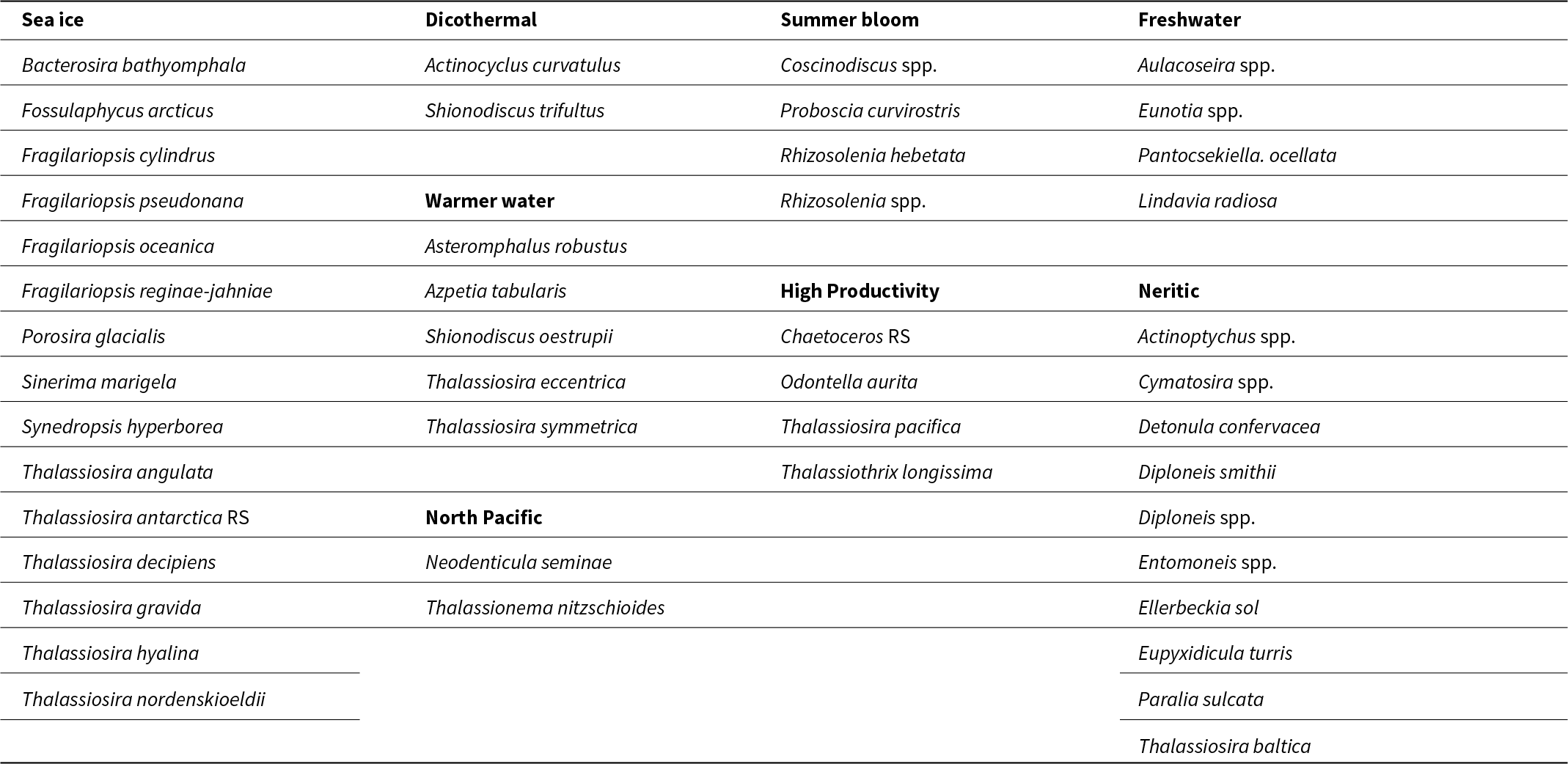
Table 2 Long description
The table categorizes diatom species observed in the study into eight environmental niches: sea ice, dicothermal waters, warmer water, North Pacific, summer bloom conditions, high productivity, freshwater and neritic. Sea ice includes multiple Fragilariopsis species, Porosira glacialis, Synedropsis hyperborea, and several Thalassiosira taxa. Dicothermal and related colder-water entries include Actinocyclus curvatulus and Shionodiscus trifultus. Warmer water species include Asteromphalus robustus, Azpeitia tabularis, Shionodiscus oestrupii, Thalassiosira eccentrica and Thalassiosira symmetrica. North Pacific associated taxa include Neodenticula seminae and Thalassionema nitzschioides. Summer bloom taxa include Coscinodiscus species, Proboscia curvirostris, and Rhizosolenia species. High productivity taxa include Chaetoceros resting spores, Odontella aurita, Thalassiosira pacifica, and Thalassiothrix longissima. Freshwater lists Aulacoseira, Eunotia, Lindavia radiosa, and Pantocsekiella ocellata. Neritic species include several benthic or nearshore genera such as Diploneis, Entomoneis, Cymatosira, and Actinoptychus.
Geochemistry
Carbon and nitrogen isotopes from 60 bulk (non-acidified) and 60 organic (acidified) sediment samples (∼1000 year temporal resolution) were measured in the Stable Isotope Lab at Iowa State University using a Delta XL Plus mass spectrometer in continuous-flow mode coupled with a Costech elemental analyzer. Before analysis, samples were ground into a fine powder using a mortar and pestle, and one set of samples was treated with 1 M HCl to remove inorganic carbon. Reference standards caffeine [IAEA-600], IAEA-N2, cellulose [IAEA-CH-3], and lab standard acetanilide were used for isotopic corrections. The combined uncertainty is ±0.08–0.11‰ (VPDB) for δ13C and ±0.13–0.21‰ (air) for δ15N.
Results
Lithology
Sediments at Site U1339 are a mix of biogenic, siliciclastic, and volcaniclastic (mostly fine ash) components (Fig. 2). Sediment is predominantly biogenic, composed largely of siliceous diatom frustules, with lesser amounts of other microfossils such as foraminifera, radiolarians, and silicoflagellates. After ∼379 ka, the biogenic content of the sediment decreases, with sediments composed of silt/clay with 10–40% diatoms (Fig. 2). Foraminifera typically have low abundances in the Bering Sea (Takahashi et al., Reference Takahashi, Ravelo and Alvarez Zarikian2011), but are present in large numbers at Site U1339 from ∼422 to 418 ka. The biogenic materials are mixed with small amounts of tephra and varying amounts of siliciclastic sediments, mostly clay and silt, but also including sand-sized minerals and rock fragments, gravel, and pebble-sized clasts that are interpreted as IRD (Fig. 2) (Takahashi et al., Reference Takahashi, Ravelo and Alvarez Zarikian2011; Thompson and Caissie, Reference Thompson and Caissie2022). Quartz grains >150 μm are consistently present throughout the record, save for the interval from 421 to 418.5 ka (Fig. 2). Ash layers are observed at ∼421.5 and ∼411 ka, but volcaniclastic material at Site U1339 is more frequently present as an accessory or trace lithology (Takahashi et al., Reference Takahashi, Ravelo and Alvarez Zarikian2011).
Lithostratigraphic column for Integrated Ocean Drilling Program (IODP) Site U1339, based on shipboard core descriptions and smear slide analyses (Takahashi et al., Reference Takahashi, Ravelo and Alvarez Zarikian2011; Thompson and Caissie, Reference Thompson and Caissie2022). Column width varies according to the median grain size of bulk sediments (Thompson and Caissie, Reference Thompson and Caissie2022). Colors represent the proportion of diatoms in the sediment: silt/clay with 10–39.9% diatoms (olive); silt/clay with 40–60% diatoms (dark green); silt/clay with >60% diatoms (yellow); laminated sediments (pale green). Blue circles indicate the presence and open circles indicate the absence of quartz grains >150 µm in the subset of samples picked for quartz grains as one proxy for ice-rafted debris (IRD). The gray side bar shows the duration of Marine Isotope Stage (MIS) 11.
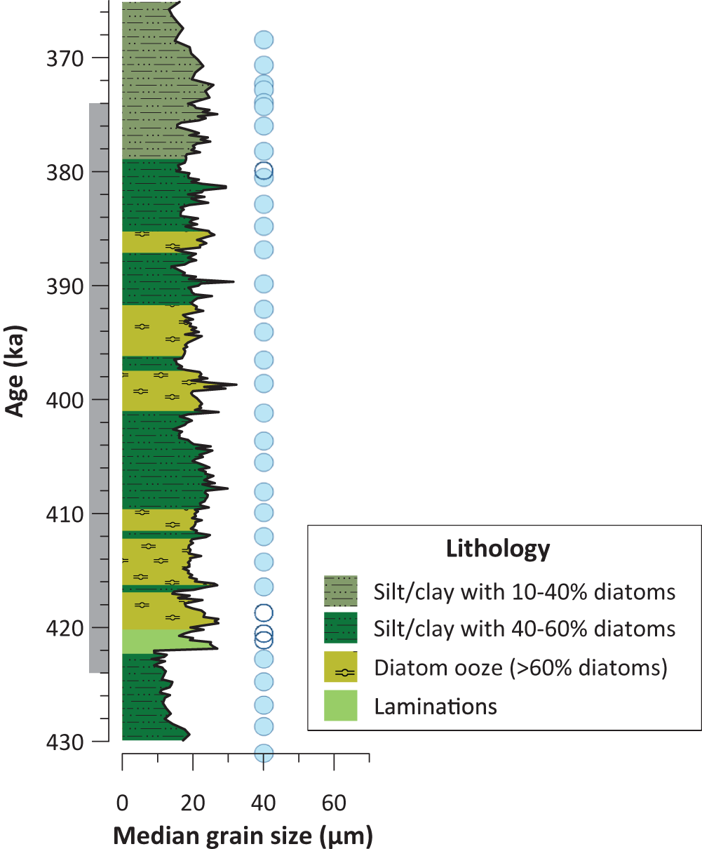
Figure 2 Long description
A vertical plot with age on the y-axis and median grain size on the x-axis. The y-axis label reads, “Age (ka).” Tick labels shown are 370, 380, 390, 400, 410, 420 and 430. The x-axis label reads, “Median grain size (micrometers)”. Tick labels shown are 0, 20, 40 and 60. A jagged black line runs vertically through the plot, varying between about 0 and 30 micrometers, with several excursions approaching about 40 micrometers. The largest excursions occur around the age labels near 420, 400, 390, and 382. A stacked lithology column fills the area to the left of the jagged line, divided into many horizontal bands with four distinct fill patterns corresponding to the legend categories. A legend box at lower right is titled, “Lithology” and lists four entries: Silt/clay with 10-40 percent diatoms; Silt/clay with 40-60 percent diatoms; Diatom ooze (greater than 60 percent diatoms); Laminations. Sediments with higher diatom percentages occur during MIS 11 rather than the glacial stages. A vertical series of circular markers is plotted to the right of the jagged line. Most circles are filled, indicating the presence of ice rafted debris, and a few are open circles, indicating the absence of ice rafted debris. The circles are placed at multiple ages from near 430 up to near 370. Most circles indicating an absences of ice rafted debris are plotted near 420 thousand years ago.
During the MIS 12–11 deglaciation, laminated sediments are deposited over a ∼2000 year interval, from 422.3 to 420.2 ka (Fig. 2). The laminated sediments consist of alternating millimeter-scale dark (more terrigenous) and light (diatom-rich) laminae (Harbour, Reference Harbour2019) and show similarities to the older laminations described by Onodera et al. (Reference Onodera, Kemp, Pearce, Horikawa and Takahashi2024) at Site U1340. Such features are most likely to be preserved under hypoxic or anoxic conditions, when oxygen concentrations at the sediment–water interface are low enough to inhibit sediment mixing by benthic organisms (Calvert, Reference Calvert, van Andel and Shor1964; Kemp, Reference Kemp1996; Pike and Kemp, Reference Pike and Kemp1999; van Geen et al., Reference van Geen, Zheng, Bernhard, Cannariato, Carriquiry, Dean, Eakins, Ortiz and Pike2003; Schimmelmann et al., Reference Schimmelmann, Lange, Schieber, Francus, Ojala and Zolitschka2016; Onodera et al., Reference Onodera, Kemp, Pearce, Horikawa and Takahashi2024).
Diatoms
Diatom assemblage
More than 90 diatom taxa were identified across 57 samples; full assemblage counts are archived at Thompson and Caissie (Reference Thompson and Caissie2025). The assemblage is dominated by resting spores (RS) of Chaetoceros Ehrenberg and Thalassiosira antarctica Comber, with smaller amounts of Fragilariopsis cylindrus (Grunow ex Cleve) Helmcke and Krieger, Thalassiosira gravida Cleve, Thalassiosira nordenskioeldii Cleve, Detonula confervacea (Cleve) Gran, Actinocyclus curvatulus Janisch, Shionodiscus trifultus (Fryxell) Alverson, Kang and Theriot, Shionodiscus oestrupii (Ostenfeld) Alverson, Kang, and Theriot, Neodenticula seminae (Simonsen and Kanaya) Akiba and Yanagisawa, Thalassionema nitzschioides (Grunow) Mereschkowsky, Coscinodiscus Ehrenberg spp., Rhizosolenia hebetata Bailey, and Thalassiosira jouseae Akiba (Fig. 3). The number of taxa per sample ranges from 29 to 51, with an average of 37 taxa.
Relative percent (area plots) and absolute (line plots with yellow dots at each sample location) abundances of diatom taxa that make up more than 10% of any assemblage. Note that we use Chaetoceros-free counts in all relative percent abundance records, with the obvious exception of Chaetoceros resting spores (RS): full counts can be found in Thompson and Caissie (Reference Thompson and Caissie2025). Taxa are grouped by environmental niche: sea ice (dark blue); neritic (brown); dicothermal (light blue); warmer water (red); North Pacific indicator (orange); summer bloom (light green); and Chaetoceros RS (dark green). The final line plot shows the total number of diatom valves per gram of sediment. Note the different scale for absolute abundances of Chaetoceros RS and all diatom valves. The gray panel indicates the duration of Marine Isotope Stage (MIS) 11 (424–374 ka), and the green bar represents laminated sediments.
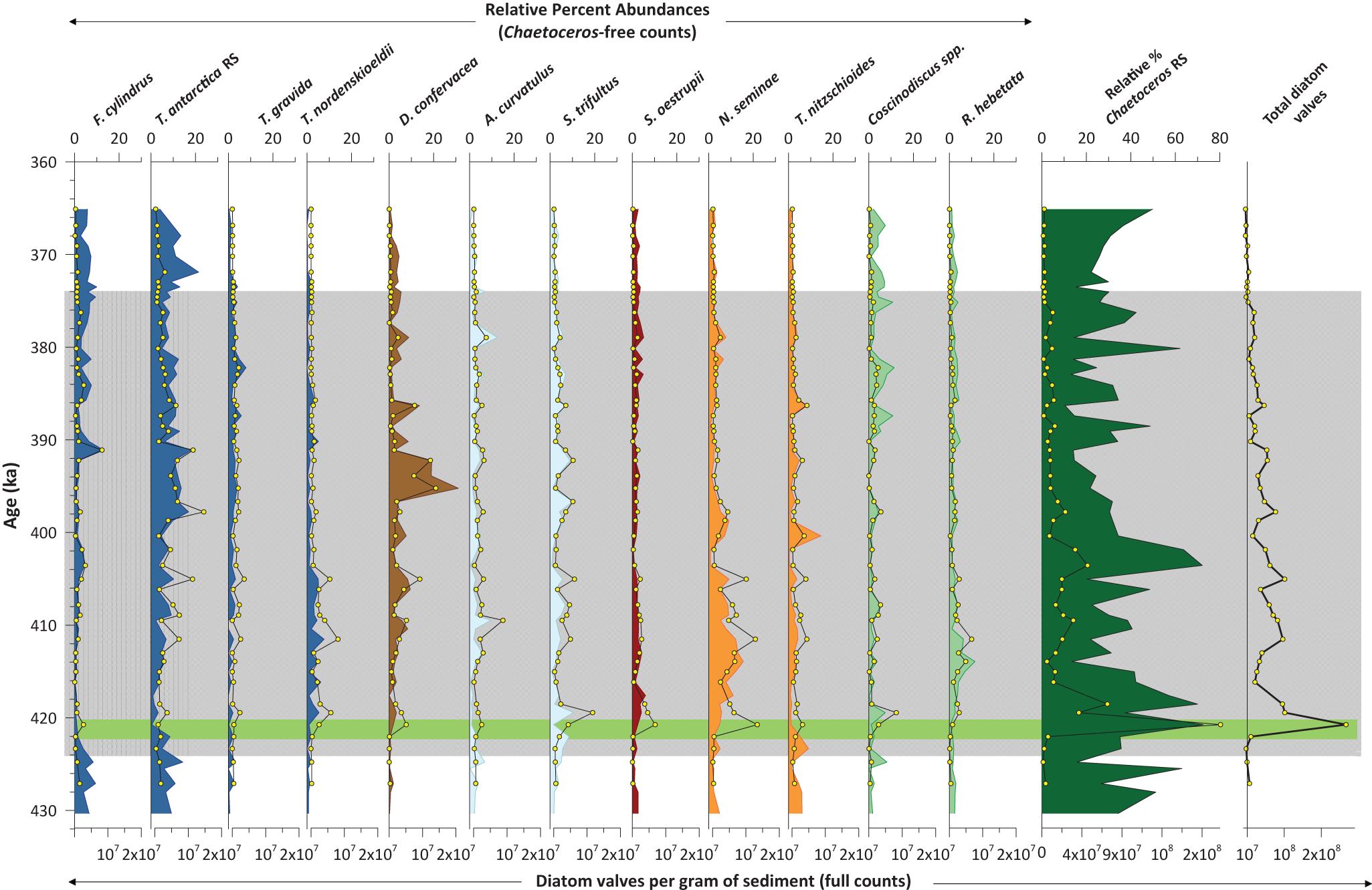
Figure 3 Long description
Fourteen aligned plots of Chaetoceros-free relative percent diatom abundances share a vertical axis labeled, “Age (ka),” with tick labels at 430, 420, 410, 400, 390, 380, 370, and 360. Plots labeled F. cylindrus, T. antarctica RS, T. gravida, T. nordenskioeldii, D. confervacea, A. curvatulus, S. trifultus, S. oestrupii, N. seminae, T. nitzschioides, Coscinodiscus spp. and R. hebetata each show relative percent abundance on the x-axis at the top, labeled with tick values 0 and 20. The plot labeled, “Relative percent Chaetoceros RS,” shows relative percent abundance on the x-axis at the top, labeled with tick values 0, 20, 40, 60 and 80. An x-axis at the bottom reads, “Diatom valves per gram of sediment (full counts),” and corresponds to the line plots overlying the relative percent abundance area plots as well as a plot to the right labeled, “Total diatom valves.” For the first 12 plots, each x-axis ranges from zero to 2 times 10 to the power of 7 with an extra tick at 10 to the power of 7. Chaetoceros RS have an x-axis that ranges from zero to 2 times 10 to the power of 8, with tick marks at 4 times 10 to the power of 7, 9 times 10 to the power of 7, and 10 to the power of 8. The final plot, “Total diatom valves,” ranges from 10 to the power of 7 to 2 times 10 to the power of 8. A horizontal shaded band spans all plots from about 424 to 374 on the Age (ka) scale, indicating MIS 11. A thinner horizontal bar spans all plots between 422 and 420 on the Age (ka) scale, indicating the presence of laminations. In general, diatoms per gram of sediment vary in sync with relative percent abundances, except for Chaetoceros RS. Variability for each species is described in the article text, but each varies between about zero and 10-20 percent. Relative percent Chaetoceros RS are most prominent, making up between 20 and 60% of the assemblage throughout MIS 11. However, the absolute abundances of Chaetoceros RS peak around 421 ka, during the laminated interval and remain much lower throughout the rest of the record. The total diatom valves line decreases across the full age range and shows a pronounced high point near the thin horizontal bar around about 421 on the, “Age (ka)” scale.
Absolute diatom abundances (total number of valves per gram of sediment) vary from 106 to 108 diatoms per gram, with values one to two orders of magnitude higher (108) during the laminated interval compared with massive intervals (Fig. 3). Diatom abundances increase during deglaciation and reach a peak during the laminated interval (420.74 ka), then gradually decline throughout the record. In general, diatom abundances are higher during MIS 11 and lowest during glacial stages 12 and 10 (Fig. 3). For the most part, absolute abundances follow the same trend as relative abundances (Fig. 3); for this reason, we focus on relative percent abundances in our interpretations.
Niche groupings
Diatoms can be valuable tools in paleoenvironmental reconstructions, because individual species have specific and unique ecological requirements with respect to temperature, salinity, and other environmental variables. In this study, we group together diatoms with similar environmental preferences to infer paleoceanographic conditions at IODP Site U1339 from MIS 12 to 10 (Table 2; modified from Caissie et al., Reference Caissie, Brigham-Grette, Cook and Colmenero-Hidalgo2016). We use Chaetoceros-free counts in the majority of our interpretations, because the extremely high abundances of Chaetoceros RS in sediments at Site U1339 dominate the assemblage and mask trends in other, less abundant species (see also Sjunneskog and Scherer, Reference Sjunneskog and Scherer1997; Leventer et al., Reference Leventer, Domack, Barkoukis, McAndrews and Murray2002; Allen et al., Reference Allen, Pike, Pudsey and Leventer2005).
Chaetoceros RS make up between 10% and 72% of the full diatom assemblage. RS of Chaetoceros are more readily preserved in sediments than Chaetoceros vegetative cells, which are weakly silicified, easily dissolved, and easily fragmented (Kanaya and Koizumi, Reference Kanaya and Koizumi1966). Relative percent abundances of Chaetoceros RS are highest during the laminated interval, with a second peak from 403.5 to 401.9 ka. Total abundances of Chaetoceros RS are strongly coupled with total diatom abundances (correlation coefficient of 0.9) (Fig. 3).
In Chaetoceros-free counts, sea ice–associated diatoms, including Bacterosira bathyomphala (Cleve) Syvertsen and Hasle, Fragilariopsis cylindrus, Fragilariopsis reginae-jahniae Witkowski, Lange-Bertalot, and Metzeltin, Fossulaphycus arcticus Blanco, Thalassiosira antarctica, Thalassiosira gravida Cleve, Thalassiosira hyalina (Grunow) Gran, and Thalassiosira nordenskioeldii, are the most abundant niche group. Sea ice diatoms comprise a large, albeit variable, proportion of the assemblage, ranging from 7% to a maximum of 62% (Fig. 4). There is a marked decline in sea ice diatoms at the onset of MIS 11, and another short-lived decline ∼400 ka, but the percentage of sea ice species does not remain low throughout MIS 11. From 417 to ∼402 ka, the relative percent abundance of the sea ice diatom group increases, with a peak centered on the interval from 403.5 to 401.9 ka. A second, short-lived peak occurs during late MIS 11 (∼391 ka), but for the most part, the percent abundance of sea ice diatoms is relatively stable after ∼398 ka (Fig. 4).
Relative percent abundances of diatoms grouped by environmental niche: neritic (brown); dicothermal (light blue); warmer water (red); North Pacific indicator (orange); high productivity (yellow); Chaetoceros resting spores (RS; dark green); and sea ice (dark blue). Note that we use Chaetoceros-free counts in all relative percent abundance records, with the obvious exception of Chaetoceros RS: full counts can be found in Thompson and Caissie (Reference Thompson and Caissie2025). Also shown is spring (March–June) sea ice concentration (including upper and lower limits) derived from a quantitative, diatom-based sea ice proxy (Nesterovich and Caissie, Reference Nesterovich and Caissie2026). Note that today, sea ice concentration at Integrated Ocean Drilling Program (IODP) Site U1339 is zero. A gray line is drawn through 50% concentration to guide the reader. The gray panel shows the duration of Marine Isotope Stage (MIS) 11 (424–374 ka), and the green bar represents laminated sediments.

Figure 4 Long description
The figure contains multiple area graphs displaying diatom percent abundances by environmental niche and sea ice concentration versus age. The x-axes represent percent abundance and range from 0-40 percent. The final x-axis represents sea ice concentration, which ranges from 0-100 percent. The y-axis shows age in thousands of years (ka) from 430 to 360 ka. 1. The first graph shows the percent abundance of neritic diatoms, ranging from 0 to 40 percent. A notable peak occurs around 395 ka. 2. The second graph displays dicothermal diatoms, fluctuating without a trend from 0 to about 20 percent. . 3. The third graph represents warmer water diatoms, with fluctuations between 0 and 15 percent. There are no noticable peaks . 4. The fourth graph shows North Pacific indicator diatoms, with values from 0 to almost 40 percent. These are generally greater than 20 percent from 430 to about 398 ka, then decrease to below 20 percent for the rest of the record. 5. The fifth graph illustrates high productivity diatoms, fluctuating between about 2 and 10 percent. 6. The sixth graph presents Chaetoceros resting spores (RS), with values from 0 to 80 percent.The largest peaks occur around 420, 418, 404-402, and 380 ka. 7. The seventh graph shows percent sea ice diatoms, ranging from 7 to about 60 percent. Although there are many fluctuations, sea ice diatoms are lowest from 426 to 410 ka. Highest values occur at 402 ka and 392 ka. 8. The final graph displays sea ice concentration, ranging from 0 to 100 percent. The line shows variability, with lowest values between 422 and 405 ka. After 404 ka, values remain above 50% for the most part. . Dotted lines indicate the 95 percent confidence interval which is about 10 percent above and below throughout.
Neritic and freshwater diatoms reflect shelf to basin transport. Freshwater diatoms make up a relatively small (0–2.3%) proportion of the assemblage at Site U1339, so they are not plotted, whereas neritic diatoms range from 2% to 42% (Fig. 4). On average, neritic diatoms comprise <10% of the assemblage, but there is an interval from ∼395 to 392 ka where the percent abundance of the neritic species D. confervacea remains consistently high (>20%) for approximately 3000 years (Fig. 3).
The dicothermal layer is a cold layer of water located between seasonally warm surface waters and warmer deep waters. In the Bering Sea today, the formation of the dicothermal layer is associated with the winter mixed layer (Miura et al., Reference Miura, Suga and Hanawa2002). Overall, the percentage of the dicothermal indicator species A. curvatulus and S. trifultus is lowest during stages 12 and 10, increases during deglaciation, and is highly variable throughout MIS 11, ranging from 3.3% to 21.9% of the assemblage (Fig. 3).
Diatoms associated with warmer water (mostly S. oestrupii) are present in relatively low abundances (<10%) for most of the record (Figs. 3 and 4). Two species (N. seminae and T. nitzschioides) are used here specifically as tracers of warm, high-nutrient, low-productivity North Pacific Water (NPW) (Abrantes et al., Reference Abrantes, Lopes, Mix and Pisias2007; Miettinen et al., Reference Miettinen, Koç and Husum2013; Lopes and Mix, Reference Lopes and Mix2018; DeLong et al., Reference DeLong, Blackburn, Caissie, Addison, Stroynowski, Sipala, Marcantionio and Ravelo2025). Although North Pacific indicator species are more abundant than warm-water diatoms, the two groups follow broadly similar trends (Fig. 4). Relative percent abundances of North Pacific indicator species increase at the onset of MIS 11, with an abrupt decline from 403.5 to 401.9 ka, consistent with a drop in the percentage of warm-water species. This is followed by a peak in North Pacific indicator species and a corresponding increase in warm-water species around 400 ka (Fig. 4).
High-productivity indicator species (mainly Odontella aurita [Lyngbye] Agardh and Thalassiothrix longissima Cleve and Grunow) are present in low abundances throughout most of the record (Fig. 4). Chaetoceros RS are also a taxon associated with high-productivity environments, but are presented separately from other high-productivity indicators, because of their association with highly productive upwelling systems (Abrantes, Reference Abrantes1988; Abrantes et al., Reference Abrantes, Lopes, Mix and Pisias2007; DeLong et al., Reference DeLong, Blackburn, Caissie, Addison, Stroynowski, Sipala, Marcantionio and Ravelo2025).
Diatom-based proxy
We used a quantitative, diatom-based proxy, based on a five species general additive model (Nesterovich and Caissie, Reference Nesterovich and Caissie2026), to estimate spring (March, April, May, June) sea ice concentrations at Site U1339. For the most part, sea ice concentrations follow the same general trend as the sea ice diatom group. Sea ice concentration is highly variable throughout the record, ranging from 7% to 89% ice cover. Sea ice concentration is mostly high (>50%) during late MIS 12, and declines with the onset of deglacial warming, reaching its lowest concentration around 413 ka, although this is by no means a linear decline. There is a peak in sea ice concentration from 403.5 to 401.9 ka, consistent with an increase in sea ice diatoms during the same interval (Fig. 4).
Geochemistry
Carbon content
Total carbon follows roughly the same trend as absolute diatom abundances, with the highest values occurring during the laminated interval, and an overall decline throughout MIS 11 (Fig. 5), indicating a strong positive relationship between diatom productivity and carbon export at Site U1339. Organic carbon (OC) values are highest (1.5%) during the laminated interval compared with an average of 0.7% for the entire record. OC declines after deglaciation, reaching a low of 0.4% by 416 ka. Overall, OC is consistently lower during MIS 12 and 10 and considerably more variable during MIS 11 (Fig. 5).
Summary of elemental and isotopic carbon and nitrogen analyses and related diatom proxies (a) percent total carbon; (b) percent organic carbon; (c) percent inorganic carbon; (d) δ13C of organic matter; (e) total diatom abundances (valves per gram); (f) relative percent abundance of Chaetoceros resting spores (RS); and (g) bulk sedimentary δ15N. The gray panel shows the duration of Marine Isotope Stage (MIS) 11 (424–374 ka), and the green bar shows laminated sediments.

Figure 5 Long description
The figure presents a multi-panel plot comparing elemental and isotopic carbon and nitrogen analyses with diatom proxies versus age. The x-axis for each panel varies, while the y-axis is the same for all and labeled, “Age (ka),” ranging from 430 to 360 ka. The gray shaded area indicates Marine Isotope Stage 11 (424–374 ka) and the green band marks laminated sediments (422-420 ka). A: Total carbon (%) shows a general decline with age, peaking at almost 3 during the laminated interval. B: Organic carbon (%) peaks at 1.5 percent during the laminated interval, then declines. C: Inorganic carbon (%) remains relatively low with isolated peaks at about 422, 418, 403, 391, and 387 ka. D: Delta 13 C (per mille VPDB) shows variability with no clear trend. The highest value is also at 422 ka during the laminated interval. E: Valves per gram (diatom abundance) peaks within the laminated interval. F: Percent Chaetoceros resting spores (RS) fluctuate throughout with the largest peaks around 420, 418, 404-402, and 380 ka, . G: Delta 15 N (per mille air) remains stable with minor fluctuations. In general, it is higher from 430 to 386 ka and lower afterward. The laminated interval corresponds to increased diatom productivity and carbon export, with notable peaks in organic carbon and diatom abundance.
Inorganic carbon (i.e., a relative measure of CaCO3; IC), is also highest during the laminated interval, consistent with an increase in foraminifera and other calcareous microorganisms (Takahashi et al., Reference Takahashi, Ravelo and Alvarez Zarikian2011). For the most part, the percent IC is lower than the percent OC, except for the interval from 391.6 to 391.1 ka, where there is a peak in IC at the same time that OC drops to its lowest value, and δ13C values become more negative. It is possible that this shift could be attributed to the presence of an authigenic carbonate nodule; authigenic dolomite, which is depleted in δ13C (Lein, Reference Lein2004), occurs as an accessory lithology at Site U1339 (Takahashi et al., Reference Takahashi, Ravelo and Alvarez Zarikian2011).
Organic matter source
Cross-plots of carbon, nitrogen, and their isotopes can be used to help identify sources of organic matter (OM) to the study site. The majority of samples comprise a mixture of terrigenous OM from soils and C3 plants, and marine OM from phytoplankton (Fig. 6). The δ13C values range from −24.8‰ to −20.4‰ VPDB, with an average value of 23.4‰ (Figs. 5 and 6). During the laminated interval, δ13C values plot closer to those of marine phytoplankton (−20‰ to −22‰) and ice algae (−18.5‰ to −20.5‰) and remain high (> − 23‰) for a period of ∼6000 years (423.7 to 417.6 ka). There is no substantial difference between the glacial and interglacial stages in terms of average δ13C, although the record is considerably variable throughout MIS 11 (Fig. 5). While OM is never fully terrigenous, there are several discrete intervals during MIS 11 when δ13C values plot close to those of terrigenous OM (−25‰ to −27‰) (Fig. 6).
Cross-plots showing (a) total organic carbon (TOC) vs. total nitrogen (TN); (b) δ13C vs. TOC/N; and (c) δ13C vs. δ15N. Gray boxes identify endmember values for likely sources of organic matter (OM) to the Bering Sea, which include marine phytoplankton (C/N: 5 to 7 [Redfield et al., Reference Redfield, Ketchum, Richards and Hill1963; Meyers, Reference Meyers1994]; δ13C: −22‰ to −19‰; and δ15N: 5‰ to 8‰ [Walinsky et al., Reference Walinsky, Prahl, Mix, Finney, Jaeger and Rosen2009]); ice algae (δ13C: −20.5‰ to −18.5‰; and δ15N: 3.5‰ to 5.5‰ [Schubert and Calvert, Reference Schubert and Calvert2001]); soil (C/N: 10–12; δ13C: −26.5‰ to −25.5‰; and δ15N: 0–1‰ [Walinsky et al., Reference Walinsky, Prahl, Mix, Finney, Jaeger and Rosen2009]); C3 vascular plants (C/N: >20 [Redfield et al., Reference Redfield, Ketchum, Richards and Hill1963; Meyers, Reference Meyers1994]; δ13C: −27‰ to −25‰ [Schubert and Calvert, Reference Schubert and Calvert2001]; and δ15N: 0–1‰ [Walinsky et al., Reference Walinsky, Prahl, Mix, Finney, Jaeger and Rosen2009]); and inorganic (clay-bound) nitrogen (δ15N: 2–4‰ [Schubert and Calvert, Reference Schubert and Calvert2001]).

Figure 6 Long description
Panel A shows a scatter plot with the y-axis labeled, “Total Nitrogen percent,” and the x-axis labeled, “Total Organic Carbon percent.” The x-axis ranges from 0 to 2. The y-axis ranges from 0 to 0.2. A legend lists MIS 10, MIS 11, and MIS 12, with dots colored based on these time periods. Text near the top reads, “r squared equals 0.71 and y equals 0.076x plus 0.05.” A fitted line slopes upward from left to right. Plotted points form a cluster mainly between Total Organic Carbon about 0.4 to 1.6 and Total Nitrogen about 0.06 to 0.17. There is no distinctive clustering of the different ages of dots. Panel B shows a scatter plot with the y-axis labeled, “TOC over N” and the x-axis labeled, “delta 13 C (per mille VPDB).” The x-axis ranges from negative 28 to negative 20. The y-axis ranges from 0 to 12. Text near the lower left reads, “r squared equals 0.22 and y equals 0.91x plus 27.78.” A fitted line slopes upward from left to right. Two labeled boxes read, “Soil,” and “Marine algae.” If you drew a line between these boxes it would cross the trend line in the scatter plot roughly perpendicularly. Plotted points form a cluster mainly between delta 13 C about negative 24.5 to negative 21.5 and TOC over N about 4 to 9, with a few points near 2 TOC over N and a few near 10 to 11 TOC over N. Panel C shows a scatter plot with the y-axis labeled, “delta 15 N (per mille air)” and the x-axis labeled, “delta 13 C (per mille VPDB).” The x-axis ranges from negative 28 to negative 18. The y-axis ranges from 0 to 8. Labeled boxes read, “Inorganic nitrogen”, “Soil/C3 plants”, “Marine algae”, and “Sea ice algae.” Plotted points form a vertically exaggerated cluster mainly between negative 24.5 to negative 21.5 delta 13 C and 3 to 7 delta 15 N, with a few points near 1 to 2 delta 15 N. Points overlap the inorganic nitrogen box and a few points fall within the marine algae box, but otherwise there is no clear carbon source.
Bulk sedimentary δ15N values range from 0.8‰ to 7.3‰ (Fig. 5). On average, δ15N is slightly lower during MIS 12 and 10 (4.7‰ and 4.3‰, respectively) compared with an average of 5‰ during MIS 11. After ∼387 ka, there are several large and irregular excursions toward both high and low δ15N values (Fig. 5). Bulk sediments may contain a substantial fraction of inorganic nitrogen adsorbed onto clay particles or incorporated into the crystal lattice of potassium-rich clays such as illite. This is a common occurrence in Arctic sediments, which typically have a high illite content (Schubert and Calvert, Reference Schubert and Calvert2001; Drenzek et al., Reference Drenzek, Montluçon, Yunker, Macdonald and Eglinton2007; Stein, Reference Stein2008). The presence of inorganic nitrogen complicates the interpretation of nitrogen records, because it lowers C/N ratios and δ15N values. A regression analysis (Fig. 6a) shows that OC is strongly positively correlated with total nitrogen (r 2 = 0.71), but the positive y-intercept (0.05) indicates that sediments at Site U1339 contain a sizable fraction of inorganic nitrogen (Schubert and Calvert, Reference Schubert and Calvert2001). The y-intercept remains positive when plotted separately for MIS 12, 11, and 10, so no single interval is without the influence of inorganic nitrogen. The presence of inorganic nitrogen is also seen in the cross-plot of δ13C versus total organic C/N (Fig. 6b). Without the complicating factor of inorganic nitrogen, we would expect to see a negatively sloping trend line reflecting mixing between the marine and terrestrial endmembers. Instead, the samples have a positive slope, due to the low C/N ratios. The low (2–4‰) δ15N values associated with clay-bound nitrogen may result in samples having a lower δ15N signal than expected in comparison to mean ocean δ15N of ∼5‰ (Sigman et al., Reference Sigman, Altabet, McCorkle, Francois and Fischer2000). Conversely, the process of denitrification, which is widespread today in the Bering Sea, can leave the nitrate pool enriched in δ15N, which ultimately results in higher (>5.5‰) sedimentary δ15N values (Brunelle et al., Reference Brunelle, Sigman, Cook, Keigwin, Haug, Plessen, Schettler and Jaccard2007). The highly variable nitrogen values at site U1339 are likely driven by a combination of denitrification and the presence of inorganic nitrogen. We therefore conclude that bulk sedimentary nitrogen is not a reliable proxy for OC source (marine vs. terrestrial) or nitrogen utilization at Site U1339.
Discussion
Sea ice at the Umnak Plateau
Sea ice history
MIS 12 (474–424 ka) is considered one of the most severe glaciations of the Quaternary (McManus et al., Reference McManus, Oppo and Cullen1999; Stein, Reference Stein2008; Rodrigues et al., Reference Rodrigues, Alonso-García, Hodell, Rufino, Naughton, Grimalt, Voelker and Abrantes2017; Koutsodendris et al., Reference Koutsodendris, Kousis, Peyron, Wagner and Pross2019). During late MIS 12 (430–424 ka in this record), insolation, atmospheric CO2, and sea level begin to increase, with sea level fluctuating around the −50 m Bering Strait sill depth until the deglaciation at 425–420 ka (Fig. 7). Both diatom assemblages and the diatom proxy indicate a period of relatively high spring ice cover (>60%) during this time, implying a longer duration of seasonal sea ice. Grain-size analyses (Thompson and Caissie, Reference Thompson and Caissie2022; Fig. 7) show that the relative proportion of terrigenous clay is highest during MIS 12, whereas the relative proportion of coarse (>150 µm) terrigenous grains, interpreted as IRD, is low. Sea ice is known to transport terrigenous clay, so it could be tempting to attribute the increase in clay-sized grains to enhanced ice-rafting during glacials. However, it has been shown that glacial periods were both drier and dustier (McGee et al., Reference McGee, Broecker and Winckler2010), which could also result in increased clay during glacials through enhanced aeolian transport. Low proportions of coarse IRD may indicate thick, perennial ice cover at Site U1339 during MIS 12, with reduced melting and thus limited deposition of sediments entrained within the ice. If this were the case, however, we would expect to see much lower sedimentation rates during MIS 12 (e.g., Nørgaard-Pedersen et al., Reference Nørgaard-Pedersen, Spielhagen, Erlenkeuser, Grootes, Heinemeier and Knies2003). Instead, MIS 12 was likely characterized by extensive seasonal sea ice, similar to the conditions at Umnak Plateau Site 51JPC during the LGM (Sancetta et al., Reference Sancetta, Heusser, Labeyrie, Naidu and Robinson1985; Caissie et al., Reference Caissie, Brigham-Grette, Lawrence, Herbert and Cook2010). In addition, the IRD content of sea ice at Site U1339 might reveal a relationship between sea ice rafting and sea level. During MIS 12, when sea level was 120–140 m below present (Rohling et al., Reference Rohling, Fenton, Jorissen, Bertrand, Ganssen and Caulet1998, Reference Rohling, Foster, Grant, Marino, Roberts, Tamisiea and Williams2014; Spratt and Lisiecki, Reference Spratt and Lisiecki2016), the area of shallow continental shelf over which sea ice forms was substantially reduced. We suggest that sea ice likely formed over deeper waters and subsequently entrained less coarse terrigenous material. At the same time, the arid, windy, and dusty glacial climate conditions allowed for increased transport of fine-grained windblown particles to the site (McGee et al., Reference McGee, Broecker and Winckler2010).
Summary of sea ice records from Integrated Ocean Drilling Program (IODP) Site U1339 compared with global records. (a) Mean monthly insolation at 65°N (Laskar et al., Reference Laskar, Robutel, Joutel, Gastineau, Correia and Levrard2004); (b) atmospheric CO2 from Antarctic ice cores (Bereiter et al., Reference Bereiter, Eggleston, Schmitt, Nehrbass-Ahles, Stocker, Fischer, Kipfstuhl and Chappellaz2015); (c) relative sea level (Red Sea) in meters above present (proxy for global sea level) (Rohling et al., Reference Rohling, Braun, Grant, Kucera, Roberts, Siddall and Trommer2010); the dashed vertical line shows the Bering Strait sill depth. (d) Volume percent terrigenous clay-sized grains (Thompson and Caissie, Reference Thompson and Caissie2022); (e) ice-rafted debris (IRD) proxies, including percent terrigenous particles >150 µm (dark blue line) (Thompson and Caissie, Reference Thompson and Caissie2022), and occurrence of quartz grains >150 µm in the subset of samples picked for quartz grains (open circles show samples devoid of quartz grains); (f) sea ice concentration from diatom-based proxy (Nesterovich and Caissie, Reference Nesterovich and Caissie2026). Vertical blue lines indicate the cutoff for unconsolidated ice (15–40% concentration) and consolidated ice (>40% concentration); values less than 15% suggest open ocean conditions; (g) relative percent abundance of sea ice diatoms; and (h) relative percent abundance of North Pacific indicator species. The gray panel shows the duration of Marine Isotope Stage (MIS) 11, and colored side bars denote the following substages: deglaciation (424–420 ka, turquoise), peak MIS 11 (430–398 ka, red), and late MIS 11 (398–374 ka, blue). The green bar represents laminated sediments.

Figure 7 Long description
The image contains multiple graphs displaying various environmental variables over time. The y-axis represents age in thousands of years (ka) from 370 to 430 ka. Graph A shows insolation at 65°N in watts per square meter, with fluctuations indicating cyclical patterns. Graph B displays atmospheric carbon dioxide levels in parts per million by volume, ranging from 175 to 275, showing a general decrease over time. Graph C illustrates relative sea level in meters, with values from negative 120 to 0, showing a rise starting around 428 ka until 400 ka, then a gradual decrease for the rest of the record. Graph D presents the percentage of terrigenous clay, with values fluctuating between 0 and 20 percent. Graph E shows ice-rafted debris (IRD) as a percentage of particles greater than 150 micrometers, with peaks indicating increased IRD. There are abundant peaks between 418 and 380 ka. Graph F depicts sea ice concentration, with values from 0 to 100 percent. The lowest values are between 422 and 405 ka. After 404 ka, values remain above 50% for the most part. Dotted lines indicate the 95 percent confidence interval which is about 10 percent above and below throughout. Graph G displays the percentage of sea ice diatoms, ranging from 0 to 60 percent. Although there are many fluctuations, sea ice diatoms are lowest from 426 to 410 ka. Highest values occur at 402 ka and 392 ka. Graph H shows the percentage of North Pacific diatoms, with values between 0 and 35 percent, These are generally greater than 20 percent from 430 to about 398 ka, then decrease to below 20 percent for the rest of the record.. The graphs collectively illustrate relationships between insolation, carbon dioxide, sea level and biological indicators, highlighting environmental changes over time.
Termination V (∼424 ka) marks the transition from MIS 12 to 11 and is followed by a period of deglaciation that occurs in line with rising eccentricity, insolation, and sea level (Fig. 7). Deglaciation at Site U1339 occurs between 424 and 420 ka and is marked by an interval of sea ice retreat. This is seen as a simultaneous decline in estimated sea ice concentrations and the relative percent abundance of sea ice diatoms, including a marked decrease in T. antarctica RS, a species associated with thick pack ice (Horner, Reference Horner1985; Figs. 3 and 7). This corresponds with increasing SST and a loss of summer sea ice in the Arctic Ocean (Cronin et al., Reference Cronin, Polyak, Reed, Kandiano, Marzen and Council2013, Reference Cronin, Keller, Farmer, Schaller, O’Regan, Poirier, Coxall and Dwyer2019).
The interglacial climatic optimum, hereafter referred to as MIS 11c, or peak MIS 11, extends from 420 to 398 ka (Kandiano et al., Reference Kandiano, Bauch, Fahl, Helmke, Roehl, Perez-Folgado and Cacho2012; PAGES Past Interglacials Working Group, Reference Berger, Crucifix, Hodell, Mangili, McManus, Otto-Bliesner and Pol2016), with peak warmth centered around 405 ka, consistent with the timing of peak eustatic sea level (∼410–400 ka) (Raymo and Mitrovica, Reference Raymo and Mitrovica2012). The deglacial sea ice retreat continues into MIS 11, with sea ice reaching its minimum extent around 417–413 ka (Fig. 7). From 417.5 to 410.5 ka, spring sea ice concentrations indicate a shift toward open-water conditions, implying the region was ice free year-round. Regionally, MIS 11 was warmer than today with temperate Pacific mollusks found near Nome (Kaufman and Brigham-Grette, Reference Kaufman and Brigham-Grette1993), July temperatures up to 6°C warmer than present at Lake El’gygytgyn (Melles et al., Reference Melles, Brigham-Grette, Minyuk, Nowaczyk, Wennrich, DeConto and Anderson2012), and northwestern Greenland ice free (Christ et al., Reference Christ, Rittenour, Bierman, Keisling, Knutz, Thomsen and Keulen2023). However, in contrast to Arctic Ocean and North Atlantic records (i.e., Kandiano et al., Reference Kandiano, van der Meer, Bauch, Helmke, Damsté and Schouten2016; Cronin et al., Reference Cronin, Keller, Farmer, Schaller, O’Regan, Poirier, Coxall and Dwyer2019; Thibodeau et al., Reference Thibodeau, Doherty, Alonso‐García, Band, González‐Lanchas, Not and Ren2025), spring sea ice does not remain low throughout MIS 11 in the Bering Sea. In fact, it increases during MIS 11c, implying seasonal ice expansion at a time when insolation, global temperatures, sea level (PAGES Past Interglacials Working Group, Reference Berger, Crucifix, Hodell, Mangili, McManus, Otto-Bliesner and Pol2016), and Arctic temperatures (Cronin et al., Reference Cronin, Keller, Farmer, Schaller, O’Regan, Poirier, Coxall and Dwyer2019) were at their highest. This is shown by the consistent presence of sea-ice rafted debris, a gradual increase in the relative percent abundance of sea ice diatoms, and an increase in sea ice concentrations from 413 to 401.9 ka (Fig. 7). Following a short-lived drop in sea ice at 400 ka, average sea ice concentrations of 61% signal a period of relatively high seasonal sea ice cover that persists throughout late MIS 11 (398–374 ka) and into MIS 10 (Fig. 7).
Controls on sea ice
Bering Sea climate is strongly influenced by variations in the inflow of NPW (Stabeno et al., Reference Stabeno, Schumacher, Ohtani, Loughlin and Ohtani1999, Reference Stabeno, Duffy-Anderson, Eisner, Farley, Heintz and Mordy2017; Detlef et al., Reference Detlef, Belt, Sosdian, Smik, Lear, Hall, Cabedo-Sanz, Husum and Kender2018). Today, relatively warm currents, derived from inflow of the AS and the ACC, inhibit sea ice formation in the Umnak Plateau region, but there is evidence that glacial reductions in NPW allowed for the expansion of sea ice at both the Umnak Plateau and the Bering Sea slope sites (e.g., Sancetta et al., Reference Sancetta, Heusser, Labeyrie, Naidu and Robinson1985; Caissie et al., Reference Caissie, Brigham-Grette, Lawrence, Herbert and Cook2010; Teraishi et al., Reference Teraishi, Suto, Onodera and Takahashi2016; Stroynowski et al., Reference Stroynowski, Abrantes and Bruno2017; Vaughn and Caissie, Reference Vaughn and Caissie2017; Detlef et al., Reference Detlef, Belt, Sosdian, Smik, Lear, Hall, Cabedo-Sanz, Husum and Kender2018). The strong, inverse correlation (−0.76) between relative percent abundances of sea ice diatoms and North Pacific indicator species at Site U1339 is further evidence for this relationship. During MIS 12 and 10, when sea ice is more extensive, NPW is reduced, reflected by low relative percent abundances of the North Pacific indicator species N. seminae and T. nitzschioides (Fig. 7). It is probable that low sea level during glacial stages 12 and 10 led to closure of Unimak Pass (−70 m) and other shallow eastern passes (Stabeno et al., Reference Stabeno, Reed and Napp2002; Ladd et al., Reference Ladd, Hunt, Mordy, Salo and Stabeno2005), thereby restricting inflow of the ACC and the distal end of the AS. This would have isolated the southeastern Bering Sea and promoted sea ice growth. Conversely, during deglaciation, as sea level rose above −50 m, the influx of warm Pacific waters at Site U1339 led to sea ice retreat and melting (Fig. 7). However, this somewhat simplistic interpretation is challenged by the findings of Sancetta and Silvestri (Reference Sancetta and Silvestri1984), who showed that abundances of N. seminae fluctuate on glacial–interglacial timescales after 450 ka, roughly in phase with the global oxygen isotope record, and likely track changes in nutrient concentrations in the open North Pacific (DeLong et al., Reference DeLong, Blackburn, Caissie, Addison, Stroynowski, Sipala, Marcantionio and Ravelo2025). Therefore, low abundances of North Pacific species in our records from MIS 12 and 10 may also be partially explained by overall lower abundances of N. seminae in the North Pacific Ocean during glacial periods.
If sea level were the main control on North Pacific inflow to the Bering Sea, we might reasonably expect to see increasing inflow, and a corresponding decline in sea ice, when sea level was at its highest during MIS 11c. Our records, however, show the opposite; not only is North Pacific inflow highly variable throughout MIS 11, the influence of NPW is reduced during the interglacial climatic optimum, at the same time that sea ice advances (Fig. 7). Although mesoscale variations in AS transport have been shown to affect climate and circulation on the Bering shelf (e.g., Ezer and Oey, Reference Ezer and Oey2010), it is unlikely that such variations could have reduced NPW inflow to near-glacial levels during MIS 11. Instead, we propose that the interplay between sea ice and NPW at the Umnak Plateau during MIS 11 was controlled, at least in part, by changes in the geographic position of the wintertime Aleutian Low, a semipermanent low-pressure system centered over the Aleutian Islands (Niebauer et al., Reference Niebauer, Bond, Yakunin, Plotnikov, Loughlin and Ohtani1999).
Today, sea ice extent in the Bering Sea is related to wind intensity, storm tracks, and the frequency of storms, all of which are controlled by the Aleutian Low (Overland and Pease, Reference Overland and Pease1982; Niebauer et al., Reference Niebauer, Bond, Yakunin, Plotnikov, Loughlin and Ohtani1999; Rodionov et al., Reference Rodionov, Bond and Overland2007; Katsuki et al., Reference Katsuki, Khim, Itaki, Harada, Sakai, Ikeda, Takahashi, Okazaki and Asahi2009; Stabeno et al., Reference Stabeno, Bell, Bond, Kimmel, Mordy and Sullivan2019). When the Aleutian Low is centered over the western Bering Sea, southerly winds inhibit the southward expansion of sea ice in the eastern Bering Sea; when the Aleutian Low is shifted farther east to the Gulf of Alaska, sea ice can advance (Rogers, Reference Rogers1981; Overland and Pease, Reference Overland and Pease1982; Stabeno et al., Reference Stabeno, Bell, Bond, Kimmel, Mordy and Sullivan2019). Because wind stress at the sea surface is an important driver of ocean circulation, changes in the strength of the Aleutian Low have also been shown to influence ocean circulation in the region of the North Pacific subarctic gyre, of which the AS forms the northern boundary current (e.g., Stabeno et al., Reference Stabeno, Schumacher, Ohtani, Loughlin and Ohtani1999; Pickart et al., Reference Pickart, Moore, MacDonald, Renfrew, Walsh and Kessler2009; Wills et al., Reference Wills, Battisti, Proistosecu, Thompson, Hartman and Armour2019). Accordingly, our analyses suggest that, during MIS 11, the strength and position of the Aleutian Low exerted a control on the advection of NPW to Site U1339, with increased transport of NPW occurring when the Aleutian Low moved eastward and/or intensified, due to the influence of wind stress curl.
To account for long-term trends in sea ice extent, the Aleutian Low would have to remain consistently weak or consistently strong over long (millennial) timescales. Decadal-scale variability in the Aleutian Low is recognized from instrumental data (Niebauer et al., Reference Niebauer, Bond, Yakunin, Plotnikov, Loughlin and Ohtani1999), but less is known about long-term variability in the Aleutian Low. However, principal component analysis of several Aleutian Low records from the Holocene suggests that the Aleutian Low has been intensifying since the Middle Holocene (Nagashima et al., Reference Nagashima, Addison, Irino, Omori, Yoshimura and Harada2022), implying that the Aleutian Low may persist in a single state for several thousand years.
A final consideration for sea ice advance during the peak sea level of MIS 11 relates to out-of-phase glaciations, specifically the Nome River glaciation, that has been observed across Beringia (Kaufman, Reference Kaufman1992; Brigham-Grette et al., Reference Brigham-Grette, Hopkins, Ivanov, Basilyan, Benson, Heiser and Pushkar2001; Gualtieri and Brigham-Grette, Reference Gualtieri and Brigham-Grette2001). In particular, deposition of glaciomarine sediments near Kotzebue imply that glaciers advanced in Beringia when MIS 11 sea level was at its highest (Huston et al., Reference Huston, Brigham-Grette and Hopkins1990; Pushkar et al., Reference Pushkar, Roof, Cherepanova, Hopkins and Brigham-Grette1999). These deposits overlie sediments that contain evidence for substantially warm SSTs (6–7°C above present; Pushkar at al., Reference Pushkar, Roof, Cherepanova, Hopkins and Brigham-Grette1999). This glaciation is hypothesized to be caused by a drop in insolation coupled with ample moisture (Huston et al., Reference Huston, Brigham-Grette and Hopkins1990; Pushkar et al., Reference Pushkar, Roof, Cherepanova, Hopkins and Brigham-Grette1999; Brigham-Grette et al., Reference Brigham-Grette, Hopkins, Ivanov, Basilyan, Benson, Heiser and Pushkar2001), perhaps due to decreased sea ice. It is plausible that this glaciation and related loss of insolation triggered sea ice to rebound. Although we have not found direct evidence of the Nome River glaciation in deep marine cores, it is plausible that it was responsible for carrying neritic and freshwater diatoms to the shelf–slope break during MIS 11 (Caissie et al., Reference Caissie, Brigham-Grette, Cook and Colmenero-Hidalgo2016).
Primary productivity at the Umnak Plateau
MIS 12
On glacial–interglacial timescales, changes in median grain size provide a rough estimate of changes in productivity (Aiello and Ravelo, Reference Aiello and Ravelo2012); around 23% of grain-size variability at Site U1339 can be explained by variations in diatom content (Thompson and Caissie, Reference Thompson and Caissie2022). Bulk mean grain-size records are in agreement with absolute diatom abundances and OC percent, all of which are consistently low during MIS 12 and higher during MIS 11 (Fig. 8). This is consistent with other glacial–interglacial records from the Bering Sea and North Pacific (e.g., Sancetta et al., Reference Sancetta, Heusser, Labeyrie, Naidu and Robinson1985; Brunelle et al., Reference Brunelle, Sigman, Cook, Keigwin, Haug, Plessen, Schettler and Jaccard2007; Schmittner and Galbraith, Reference Schmittner and Galbraith2008; Caissie et al., Reference Caissie, Brigham-Grette, Lawrence, Herbert and Cook2010; Riethdorf et al., Reference Riethdorf, Nürnberg, Max, Tiedemann, Gorbarenko and Malakhov2013; Vaughn and Caissie, Reference Vaughn and Caissie2017; Worne et al., Reference Worne, Kender, Swann, Leng and Ravelo2019), which suggest that glacial periods in this region are marked by low primary productivity. Today, productivity in the Bering Sea is strongly dependent upon the availability of nutrients and light, and is therefore highly seasonal (Arrigo et al., Reference Arrigo, Perovich, Pickart, Brown, van Dijken, Lowry and Mills2014). In particular, increased light availability and stratification during spring sea ice melt drives the hugely productive spring phytoplankton bloom (e.g., Niebauer et al., Reference Niebauer, Alexander and Henrichs1990; Sigler et al., Reference Sigler, Harvey, Ashijian, Lomas, Napp, Stabeno and Van Pelt2010; Brown and Arrigo, Reference Brown and Arrigo2013; Fleury et al., Reference Fleury, Martinez, Crosta, Charlier, Billy, Hanquiez, Blanz and Schneider2015; Vancoppenolle et al., Reference Vancoppenolle, Bopp, Madec, Dunne, Ilyina, Halloran and Steiner2013). If, as we suggest, sea ice was more extensive during MIS 12, algal blooms at Site U1339 would have been limited to in-ice or below-ice production, with the spring bloom occurring in the marginal ice zone farther to the south. Increased sea ice cover may have further restricted productivity in two ways. Sea ice coverage limits the effects of wind forcing, thereby reducing the formation of eddies, which drive upwelling of deep, nutrient-rich waters (Rainville et al., Reference Rainville, Lee and Woodgate2011). In addition, the formation of sea ice strengthens water-column stratification, thus limiting the flux of nutrients into the photic zone (Sigman et al., Reference Sigman, Jaccard and Haug2004). Glacial reductions in primary productivity were driven, at least in part, by this reduction of upwelled nutrients, due to the expansion of sea ice and concurrent expansion of low-nutrient North Pacific Intermediate Water (Worne et al., Reference Worne, Kender, Swann, Leng and Ravelo2019). Restricted inflow through passes between the Aleutian Islands may also have caused Bering Sea circulation to weaken and further reduced nutrient supply to the shelf edge (Reed and Stabeno, Reference Reed, Stabeno, Loughlin and Ohtani1999; Kanematsu et al., Reference Kanematsu, Takahashi, Kim, Asahi and Khim2013; Stabeno et al., Reference Stabeno, Danielson, Kachel, Kachel and Mordy2016).
Summary of productivity records from Integrated Ocean Drilling Program (IODP) Site U1339 compared with global records. (a) Mean monthly insolation at 65°N (Laskar et al., Reference Laskar, Robutel, Joutel, Gastineau, Correia and Levrard2004); (b) atmospheric CO2 from Antarctic ice cores (Bereiter et al., Reference Bereiter, Eggleston, Schmitt, Nehrbass-Ahles, Stocker, Fischer, Kipfstuhl and Chappellaz2015); (c) relative sea level (Red Sea) in meters above present (proxy for global sea level) (Rohling et al., Reference Rohling, Braun, Grant, Kucera, Roberts, Siddall and Trommer2010); the dashed vertical line shows the Bering Strait sill depth. (d) Bulk median grain size (Thompson and Caissie, Reference Thompson and Caissie2022); (e) diatom valves per gram of sediment); (f) Chaetoceros per gram of sediment; (g) relative percent abundance of Chaetoceros resting spores (RS); (h) percent organic carbon; (i) percent inorganic carbon; and (j) δ13C (‰ VPDB). Diatom percent abundances are based on Chaetoceros-free counts. The gray panel shows the duration of Marine Isotope Stage (MIS) 11, and colored side bars denote the following substages: deglaciation (424–420 ka, turquoise), peak MIS 11 (MIS 11c) (430–398 ka, red), and late MIS 11 (398–374 ka, blue). The green bar represents laminated sediments.

Figure 8 Long description
The image presents a series of ten stacked time-series plots against age in thousands of years (ka), ranging from 430 to 370 ka. Each plot represents different variables related to productivity records from the Integrated Ocean Drilling Program Site U1339. The y-axis for all plots is labeled ′Age (ka)′. The x-axes are labeled as follows: (a) Insolation at 65 degrees North in watts per meter squared, ranging from 440 to 500; (b) Atmospheric carbon dioxide in parts per million by volume, ranging from 175 to 275; (c) Relative sea level in meters, ranging from negative 120 to 0; (d) Bulk median grain size in micrometers, ranging from 0 to 30; (e) Diatoms per gram, ranging from 10 superscript 6 to slightly greater than 10 superscript 8; (f) Chaetoceros per gram, ranging from 10 superscript 6 to slightly greater than 10 superscript 8; (g) Percent Chaetoceros resting spores, ranging from 0 to 80; (h) Percent organic carbon, ranging from 0 to 2; (i) Percent inorganic carbon, ranging from 0 to 2; (j) Delta carbon thirteen in per mille Vienna Pee Dee Belemnite, ranging from negative 26 to negative 20. The plots show various trends: insolation exhibits a cyclical pattern; atmospheric carbon dioxide and relative sea level show an initial increase followed by a general decline; grain size fluctuates but in general is largest between 422 and 372 ka and lower in the glacial intervals; diatom content and absolute abundances of Chaetoceros both peak around 422 ka and then decline gradually for the rest of the record; Chaetoceros resting spores show variability with notable peaks at 420, 418, 404-402, and 380 ka; organic and inorganic carbon percentages remain relatively stable with maximum values around 422 ka; delta carbon thirteen shows slight variations. The gray shaded area marks the duration of Marine Isotope Stage 11 (424-374 ka), while the green band highlights the laminated interval (422-420 ka). Colored side bars indicate substages: deglaciation is 424-420 ka, peak MIS 11 is 430-398 ka and late MIS 11 is 398-374 ka.
Termination V
During deglaciation, as sea level rose above −50 m, Unimak Pass and the Bering Strait reopened, which led to flooding of the continental shelf and a subsequent influx of nutrients to the Bering Sea (Shiga and Koizumi, Reference Shiga and Koizumi1999; Bertrand et al., Reference Bertrand, Pedersen, Martinez, Calvert and Shimmield2000; Poli et al., Reference Poli, Meyers and Thunell2010). The combination of rising sea level, the collapse of formation of glacial North Pacific Intermediate Water (Worne et al., Reference Worne, Kender, Swann, Leng and Ravelo2019), declining sea ice cover and increased nutrient supply drove rapidly increasing productivity, culminating in the deposition of laminated sediments between 422.3 and 420.2 ka (Fig. 8). Laminated sediments are widespread features of deglacial transitions and have been shown to be varves in several studies (Kuehn et al., Reference Kuehn, Lembke-Jene, Gersonde, Esper, Lamy, Arz, Kuhn and Tiedemann2014; Onodera et al., Reference Onodera, Kemp, Pearce, Horikawa and Takahashi2024). During the last deglaciation (∼15 ka), laminae were simultaneously deposited across the North Pacific and its marginal seas (e.g., Cook et al., Reference Cook, Keigwin and Sancetta2005; Brunelle et al., Reference Brunelle, Sigman, Cook, Keigwin, Haug, Plessen, Schettler and Jaccard2007; Caissie et al., Reference Caissie, Brigham-Grette, Lawrence, Herbert and Cook2010; Addison et al., Reference Addison, Finney, Dean, Davies, Mix, Stoner and Jaeger2012; Schlung et al., Reference Schlung, Ravelo, Aiello, Andreasen, Cook, Drake and Dyez2013; Pelto et al., Reference Pelto, Caissie, Petsch and Brigham‐Grette2018). Laminated sediments have also been reported from other sites in the Bering Sea during early MIS 11 (e.g., Takahashi et al., Reference Takahashi, Ravelo and Alvarez Zarikian2011; Caissie et al., Reference Caissie, Brigham-Grette, Cook and Colmenero-Hidalgo2016; Feng et al., Reference Feng, Zou, Shi, Worne, Yao, Zhong, Jin, Dong, Feng and Zou2024). Laminated sediments typically form under low-oxygen conditions; therefore, the presence of laminated sediments at Site U1339 would have required expansion of the oxygen minimum zone, currently located between −700 and −1600 m, (Takahashi et al., Reference Takahashi, Ravelo and Alvarez Zarikian2011), to a water depth of at least 1800 m.
Although the exact causes of deglacial anoxia are still debated, leading hypotheses include changes in the ventilation of intermediate waters (Yu et al., Reference Yu, Menviel, Jin, Anderson, Jian, Piotrowski and Ma2020), increased export productivity driven by deglacial warming (Kuehn et al., Reference Kuehn, Lembke-Jene, Gersonde, Esper, Lamy, Arz, Kuhn and Tiedemann2014; Praetorius et al., Reference Praetorius, Mix, Walczak, Wolhowe, Addison and Prahl2015), or a combination of the two (Cook et al., Reference Cook, Keigwin and Sancetta2005; Matul et al., Reference Matul, Abelmann, Khusid, Chekhovskaya, Kaiser, Nürnberg and Tiedemann2016). Several lines of evidence point toward extremely high productivity at U1339 during the laminated interval, including an increase in absolute diatom abundances by two orders of magnitude over MIS 12, and a marked increase in bulk median grain size, which implies a greater contribution from silt-sized biogenic material, that is, diatoms (Aiello and Ravelo, Reference Aiello and Ravelo2012; Thompson and Caissie, Reference Thompson and Caissie2022; Fig. 8). Consistent with this, a peak in δ13C values suggests that OM is primarily sourced from marine phytoplankton during this time. In addition, an increase in both OC and IC during the laminated interval indicates high rates of productivity across multiple phytoplankton groups, including calcareous organisms such as foraminifera and calcareous nannofossils (Takahashi et al., Reference Takahashi, Ravelo and Alvarez Zarikian2011). At U1339 and other sites in the Bering Sea, MIS 11 laminations display the most intense dysoxygenation of the past 800 ka coupled with extremely high productivity (Feng et al., Reference Feng, Zou, Shi, Worne, Yao, Zhong, Jin, Dong, Feng and Zou2024).
MIS 11
In general, primary productivity declines over the course of MIS 11, as shown by gradually decreasing diatom abundances and an overall decrease in OC (Fig. 8). Median grain size remains higher throughout MIS 11, not because productivity is consistently high, but because the grain size of bulk sediments is also influenced by the input of coarser, ice-rafted material.
During MIS 11, when sea ice is extensive, productivity can be either low or high (Figs. 7 and 8), which indicates that the relationship between sea ice and productivity is far more complex than the assumption that sea ice inhibits productivity. As described previously, there is a massive flux of nutrients during deglaciation, when sea-level rise floods the Bering Shelf; however, this influx of nutrients is not sustained throughout MIS 11, and it may be that productivity declines as nutrients become gradually depleted during MIS 11. Pelto et al. (Reference Pelto, Caissie, Petsch and Brigham‐Grette2018) hypothesized that productivity at the Umnak Plateau remains high until the Bering Strait is fully submerged, because until that point, nutrients remain trapped in the Bering Sea. Once the strait is flooded, however, Bering shelf waters can transport nutrients from the Bering Sea northward into the Chukchi Sea, as they do today (Cooper et al., Reference Cooper, Whitledge, Grebmeier and Weingartner1997; Tremblay et al., Reference Tremblay, Anderson, Matrai, Coupel, Bélanger, Michel and Reigstad2015).
Chaetoceros RS are indicators of both high productivity and upwelling, because Chaetoceros only blooms when nutrient levels are high enough to sustain multiple diatom blooms each year, or when there is an input of nutrients later in the year to support a second bloom (Abrantes, Reference Abrantes1988; Abrantes et al., Reference Abrantes, Lopes, Mix and Pisias2007). At Site U1339, Chaetoceros RS tell a different story to other productivity indicators. Absolute abundances of Chaetoceros RS are closely coupled with absolute diatom abundances (Fig. 8), simply because Chaetoceros RS dominate the assemblage, but the relative percent abundance of Chaetoceros RS fluctuates throughout MIS 11, independent of both sea ice and other productivity indicators. We conclude that down-core variations in Chaetoceros RS likely reflect changes in upwelling, but productivity increases may occur due to upwelled nutrients or other factors such as the flooding of the Bering Shelf or deglacial warming.
Summary
In this study, we described changes in sea ice extent and primary productivity at the Umnak Plateau (Site U1339) during the MIS 12–10 cycle. Similar to the LGM, MIS 12 was likely characterized by extensive, seasonal sea ice over the Umnak Plateau. We did not find evidence for perennial ice in this region, but high sea ice concentrations indicate a longer annual duration of seasonal ice.
Sea ice declined during deglaciation and at the beginning of MIS 11, with a shift toward unconsolidated ice and likely year-round open-water conditions starting around 417.5 ka and lasting for several thousand years. However, sea ice did not remain low throughout MIS 11. Instead, we see evidence that sea ice readvanced over the Umnak Plateau during the latter half of MIS 11c, when global temperatures and sea level were still high, but the influence of warm NPW was reduced. In contrast, today, sea ice has been absent from the Umnak Plateau region since the Holocene thermal maximum (∼8 ka) (Nesterovich and Caissie, Reference Nesterovich and Caissie2026). The interplay between sea ice extent and NPW during MIS 11 was likely controlled, at least in part, by persistent changes in the geographic position and intensity of the Aleutian Low.
In general, productivity at Site U1339 was high during MIS 11 and lowest during glacial stages 12 and 10. Similar to the last deglaciation, laminated sediments were deposited during the transition from MIS 12 to 11. Multiple lines of evidence indicate a spike in productivity during the deposition of the laminated sediments. The gradual decline in productivity over the course of MIS 11 occurred independently of fluctuating sea ice, which suggests that productivity was controlled by more complex factors than simply changing sea ice extent. Nutrient availability may have become a limiting factor as MIS 11 progressed.
Acknowledgments
We thank the captain and crew of the JOIDES Resolution and IODP Expedition 323 science party, especially co–chief scientists Christina Ravelo and Kozo Takahashi. We also thank Chris Beck and Courtney Schill for their assistance with diatom slide counts, and Kate Staebell for her assistance with grain-size analysis. NST acknowledges a graduate research grant from the Geological Society of America, and BEC acknowledges funding from the USGS Ecosystems Mission Area Land Change Science Program and NSF grant no. 2110923 to UCSC. The authors are grateful to two anonymous reviewers as well as USGS reviewers Clarke Knight, Scott Starratt, and Laura Gemery for improving our article and ensuring that our data, biologic, and geologic names are accurate. Any use of trade, firm, or product names is for descriptive purposes only and does not imply endorsement by the U.S. Government.
Data availability statement
All diatom and stable isotope data have been archived at the National Centers for Environmental Information Paleoclimatology Data archive: https://doi.org/10.25921/rdmd-wz81.
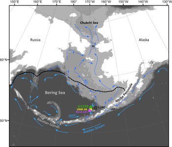
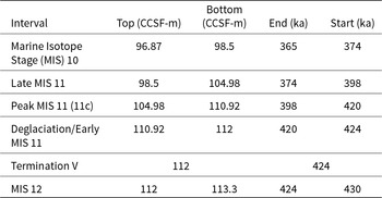
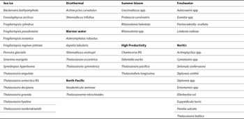
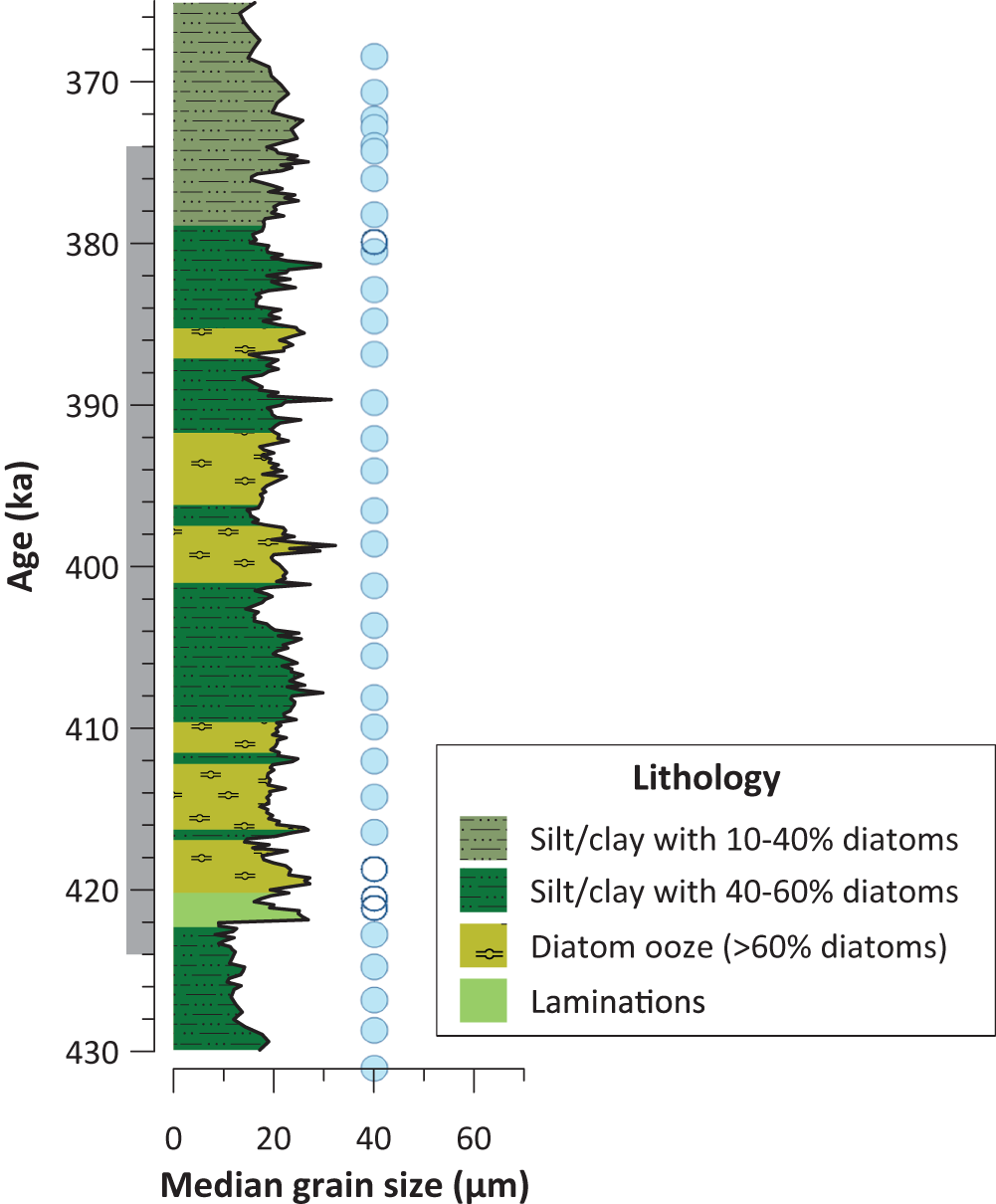
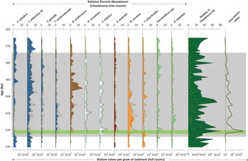
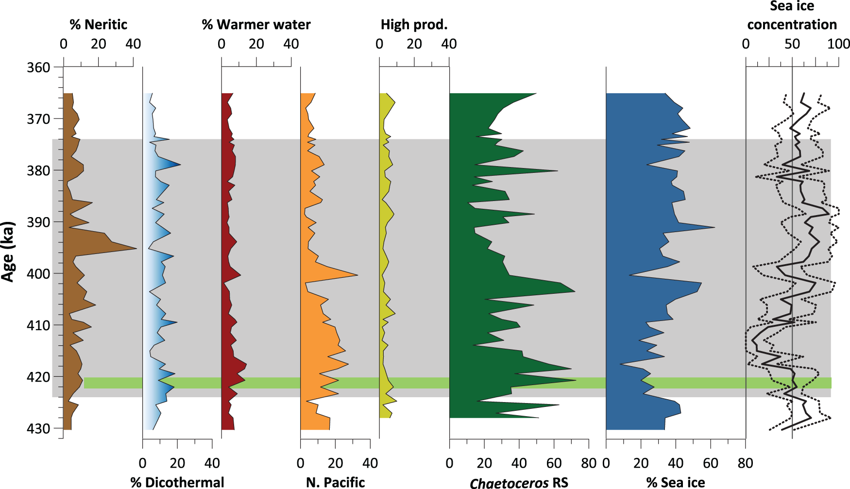
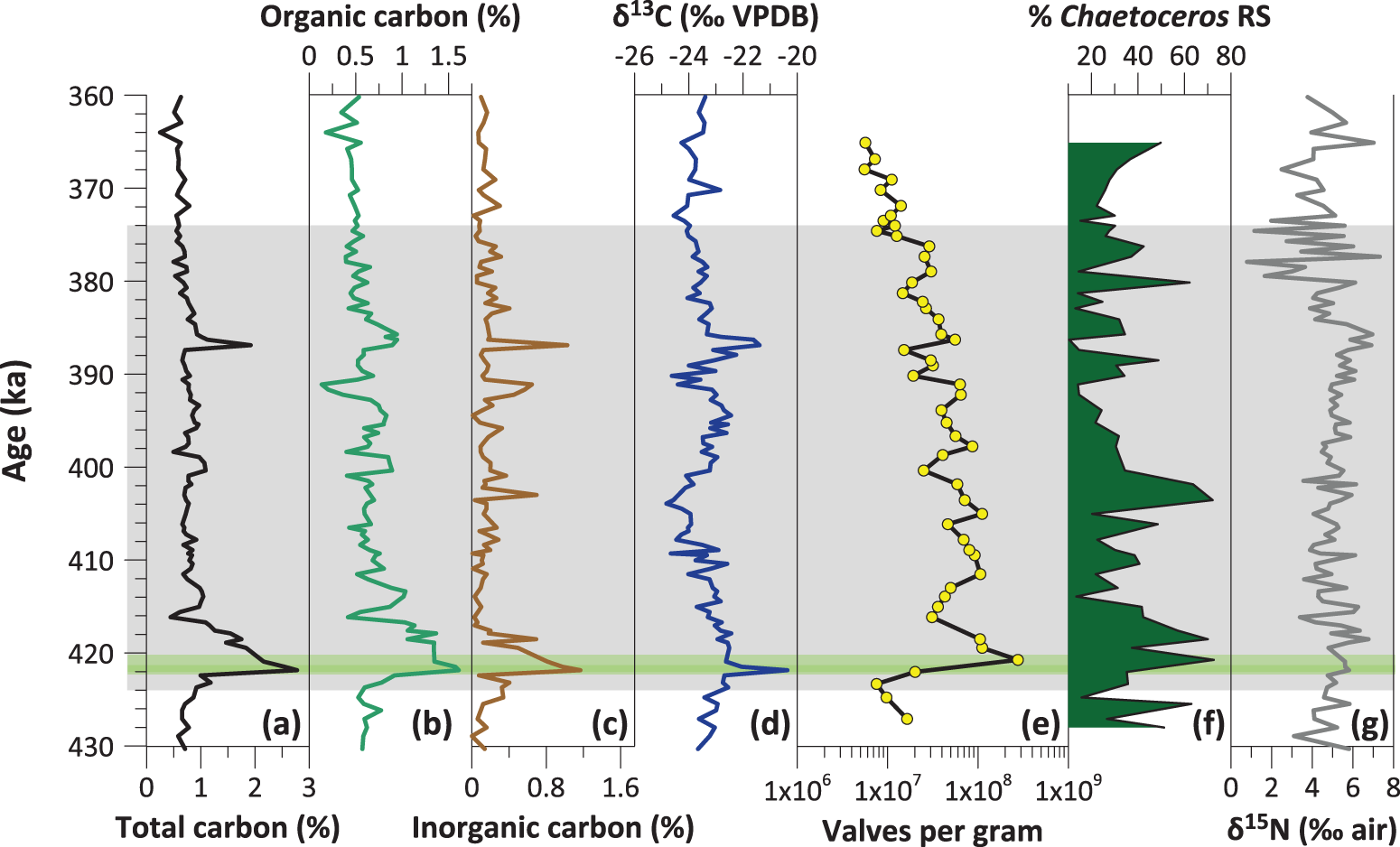
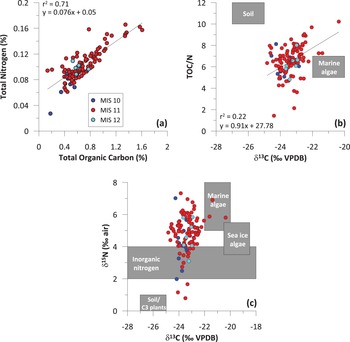
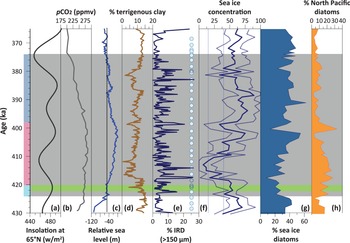


 Open access

