





1. Introduction
The present work explores the influence of structural damping on vortex-induced vibrations (VIV). VIV are a form of flow-induced vibrations ubiquitous in nature and with direct impact on the fatigue life of engineering structures (Williamson & Govardhan Reference Williamson and Govardhan2004). These vibrations are driven by a synchronisation, or lock-in, between body motion and flow unsteadiness associated with vortex formation in the wake. A circular cylinder, free to oscillate within a uniform cross-current, represents a canonical problem to study the fluid–structure interaction mechanisms involved in the development of VIV. This canonical problem is considered here.
For a cylinder moving along a rectilinear path normal to the current, with or without structural restoring force (SRF), the peak amplitudes of VIV, of the order of one body diameter, tend to decrease as structural damping is increased (Feng Reference Feng1968; Hover, Miller & Triantafyllou Reference Hover, Miller and Triantafyllou1997; Khalak & Williamson Reference Khalak and Williamson1997; Govardhan & Williamson Reference Govardhan and Williamson2006; Klamo, Leonard & Roshko Reference Klamo, Leonard and Roshko2006; Soti et al. Reference Soti, Thompson, Sheridan and Bhardwaj2017; Han et al. Reference Han, de Langre, Thompson, Hourigan and Zhao2023). When structural damping is increased from zero, the persistence of VIV requires an increase in energy transfer from the fluid to the structure, to balance energy dissipation. Under a harmonic motion assumption, which is often acceptable in this context, some insights into the effect of an increase in energy transfer can be gained from the energy maps obtained via forced sinusoidal oscillations of the cylinder, at prescribed amplitudes and frequencies (Hover, Techet & Triantafyllou Reference Hover, Techet and Triantafyllou1998; Morse & Williamson Reference Morse and Williamson2009; Baranyi & Daróczy Reference Baranyi and Daróczy2013; Kumar, Navrose & Mittal Reference Kumar and Mittal2016). In the region of large-amplitude oscillations, an increase in energy transfer implies a reduction in amplitude, which is actually observed for the peak amplitudes of VIV. However, a different trend can be identified at lower amplitudes: forced oscillation results show that the energy transfer can increase with the amplitude. This trend, and therefore the possible enhancement of VIV by structural damping, motivated the present study. Beyond the fundamental aspects addressed hereafter, the counterintuitive amplifying effect of structural damping may have practical implications, for example in applications where damping is expected to attenuate the vibrations or is employed to harvest energy from fluid flows.
The exploration of the effect of structural damping is conducted as follows, on the basis of numerical simulations. As a first step, focus is placed on rectilinear VIV without SRF. Without damping, or with a low level of damping, the peak amplitudes are concentrated in a range of low values of the structure to displaced fluid mass ratio ( $m^\star$
), typically
$m^\star$
), typically $m^\star \lt 0.5$
(Shiels, Leonard & Roshko Reference Shiels, Leonard and Roshko2001; Govardhan & Williamson Reference Govardhan and Williamson2002; Ryan, Thompson & Hourigan Reference Ryan, Thompson and Hourigan2005; Navrose & Mittal Reference Mittal2017; Bourguet Reference Bourguet2023, Reference Bourguet2025). It appears that the vibrations developing beyond this range of
$m^\star \lt 0.5$
(Shiels, Leonard & Roshko Reference Shiels, Leonard and Roshko2001; Govardhan & Williamson Reference Govardhan and Williamson2002; Ryan, Thompson & Hourigan Reference Ryan, Thompson and Hourigan2005; Navrose & Mittal Reference Mittal2017; Bourguet Reference Bourguet2023, Reference Bourguet2025). It appears that the vibrations developing beyond this range of $m^\star$
visit the region of the amplitude–frequency domain where forced oscillation maps suggest a possible enhancement by damping. This enhancement is analysed over ranges of values of
$m^\star$
visit the region of the amplitude–frequency domain where forced oscillation maps suggest a possible enhancement by damping. This enhancement is analysed over ranges of values of $m^\star$
and of the Reynolds number (
$m^\star$
and of the Reynolds number ( $\textit{Re}$
), based on the body diameter and current velocity. VIV arise below the critical
$\textit{Re}$
), based on the body diameter and current velocity. VIV arise below the critical $\textit{Re}$
threshold of
$\textit{Re}$
threshold of $47$
that marks the onset of flow unsteadiness for a fixed cylinder (e.g. Cossu & Morino Reference Cossu and Morino2000; Ryan et al. Reference Ryan, Thompson and Hourigan2005; Bourguet Reference Bourguet2023). The subcritical-
$47$
that marks the onset of flow unsteadiness for a fixed cylinder (e.g. Cossu & Morino Reference Cossu and Morino2000; Ryan et al. Reference Ryan, Thompson and Hourigan2005; Bourguet Reference Bourguet2023). The subcritical- $\textit{Re}$
range is included in the analysis, to clarify the impact of damping on vibration onset. Then, in order to examine the generality of the results, the investigation is extended to curved trajectories and to a system with SRF.
$\textit{Re}$
range is included in the analysis, to clarify the impact of damping on vibration onset. Then, in order to examine the generality of the results, the investigation is extended to curved trajectories and to a system with SRF.
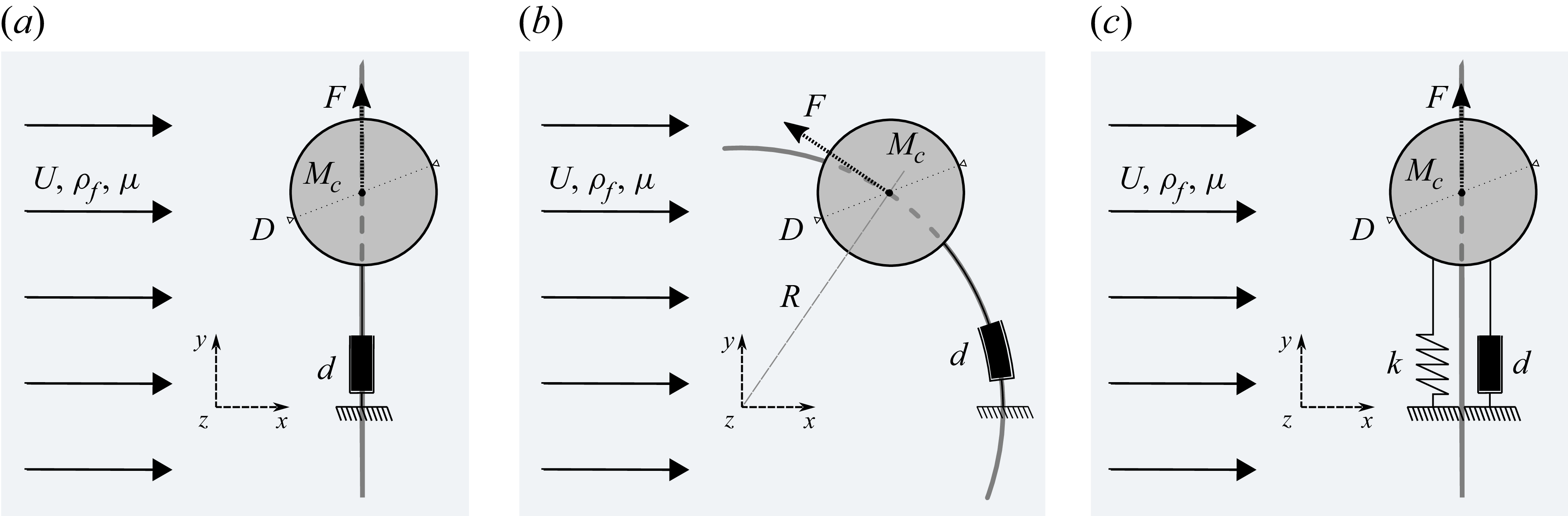
Schematics of the configurations: (a) rectilinear path with damping, (b) curvilinear path with damping and (c) rectilinear path with damping and elastic support.

Figure 1. Long description
Panel A: Diagram of a cylinder moving along a rectilinear path with damping. The cylinder is labeled Mc, with a diameter D, and is attached to a damping element labeled d. The fluid flow is represented by horizontal arrows labeled U, rho_f, and mu. A force F acts on the cylinder. The coordinate axes are labeled x, y, and z. Panel B: Diagram of a cylinder moving along a curvilinear path with damping. The cylinder is labeled Mc, with a diameter D, and is attached to a damping element labeled d via a flexible connection labeled R. The fluid flow is represented by horizontal arrows labeled U, rho_f, and mu. A force F acts on the cylinder. The coordinate axes are labeled x, y, and z. Panel C: Diagram of a cylinder moving along a rectilinear path with damping and elastic support. The cylinder is labeled Mc, with a diameter D, and is attached to a damping element labeled d and an elastic support labeled k. The fluid flow is represented by horizontal arrows labeled U, rho_f, and mu. A force F acts on the cylinder. The coordinate axes are labeled x, y, and z.
2. Formulation and numerical method
Schematics of the physical configurations are presented in figure 1. In all cases, the circular cylinder of diameter $D$
and mass per unit length
$D$
and mass per unit length $M_c$
is parallel to the
$M_c$
is parallel to the $z$
axis and placed in an incompressible uniform current of velocity
$z$
axis and placed in an incompressible uniform current of velocity $U$
, density
$U$
, density $\rho _{\!f}$
, viscosity
$\rho _{\!f}$
, viscosity $\mu$
, aligned with the
$\mu$
, aligned with the $x$
axis. It is mounted on a support of damping per unit length
$x$
axis. It is mounted on a support of damping per unit length $d$
. A SRF can be added via an elastic support of stiffness per unit length
$d$
. A SRF can be added via an elastic support of stiffness per unit length $k$
. The cylinder is free to translate either along the
$k$
. The cylinder is free to translate either along the $y$
axis, or along a circular path of radius
$y$
axis, or along a circular path of radius $R$
, parallel to the
$R$
, parallel to the $(x,y)$
plane. The rectilinear path corresponds to the limiting case of the curvilinear path where
$(x,y)$
plane. The rectilinear path corresponds to the limiting case of the curvilinear path where $R$
tends to infinity. The physical variables are non-dimensionalised by
$R$
tends to infinity. The physical variables are non-dimensionalised by $\rho _{\!f}$
,
$\rho _{\!f}$
, $D$
and
$D$
and $U$
. The non-dimensional curvature of the path is defined as
$U$
. The non-dimensional curvature of the path is defined as $\kappa =D/R$
;
$\kappa =D/R$
; $\kappa =0$
for the rectilinear path. The cylinder displacement along the rectilinear (figure 1
a,c) or circular (figure 1
b) path, non-dimensionalised by
$\kappa =0$
for the rectilinear path. The cylinder displacement along the rectilinear (figure 1
a,c) or circular (figure 1
b) path, non-dimensionalised by $D$
, is denoted by
$D$
, is denoted by $\zeta$
. The force coefficient is defined as
$\zeta$
. The force coefficient is defined as $C=2F/(\rho _{\!f} D U^2)$
, where
$C=2F/(\rho _{\!f} D U^2)$
, where $F$
is the dimensional fluid force per unit length aligned with the direction of motion. The dynamics of the cylinder is governed by the following equations:
$F$
is the dimensional fluid force per unit length aligned with the direction of motion. The dynamics of the cylinder is governed by the following equations:
 \begin{align} &\text{- without SRF}\,\,\,\,\, \ddot \zeta + {4\pi \textit{St}\xi } \dot \zeta = \dfrac {2 C}{\pi m^\star }, \\[-12pt]\nonumber \end{align}
 \begin{align} &\text{- with SRF}\,\,\,\, \ddot \zeta + {4\pi f_n \xi _s} \dot \zeta + \left ({2\pi f_n}\right )^2 \zeta = \dfrac {2 C}{\pi m^\star }, \end{align}
where $\dot {\phantom {a}}$
designates the non-dimensional time derivative. The structure to displaced fluid mass ratio, structural damping ratio without SRF and with SRF, non-dimensional natural frequency and associated reduced velocity are defined as
$\dot {\phantom {a}}$
designates the non-dimensional time derivative. The structure to displaced fluid mass ratio, structural damping ratio without SRF and with SRF, non-dimensional natural frequency and associated reduced velocity are defined as $m^\star =4 M_c/(\pi \rho _{\!f} D^2)$
,
$m^\star =4 M_c/(\pi \rho _{\!f} D^2)$
, $\xi =d D/(4\pi \textit{St} \textit{UM}_c)$
,
$\xi =d D/(4\pi \textit{St} \textit{UM}_c)$
, $\xi _s=d/(2\sqrt {k M_c})$
,
$\xi _s=d/(2\sqrt {k M_c})$
, $f_n=[D/(2\pi U)]\sqrt {k/M_c}$
and
$f_n=[D/(2\pi U)]\sqrt {k/M_c}$
and $U^\star =1/f_n$
, respectively. Without SRF, in the absence of stiffness to define a critical damping, the structural damping ratio is based on the frequency of vortex shedding measured when the cylinder is fixed, as suggested by Govardhan & Williamson (Reference Govardhan and Williamson2002); the Strouhal frequency (
$U^\star =1/f_n$
, respectively. Without SRF, in the absence of stiffness to define a critical damping, the structural damping ratio is based on the frequency of vortex shedding measured when the cylinder is fixed, as suggested by Govardhan & Williamson (Reference Govardhan and Williamson2002); the Strouhal frequency ( $St$
) designates the non-dimensional value of this vortex shedding frequency. For more clarity, the damping ratio based on
$St$
) designates the non-dimensional value of this vortex shedding frequency. For more clarity, the damping ratio based on $St$
is also used for the system with SRF in the presentation of the results (
$St$
is also used for the system with SRF in the presentation of the results ( $\xi _s={ St} U^\star \xi$
).
$\xi _s={ St} U^\star \xi$
).
The Reynolds number, $\textit{Re}=\rho _{\!f} \textit{UD}/\mu$
, is varied from subcritical values to
$\textit{Re}=\rho _{\!f} \textit{UD}/\mu$
, is varied from subcritical values to $160$
, which ensures that the flow remains two-dimensional across the parameter space investigated. This point has been verified via three-dimensional simulations. The two-dimensional Navier–Stokes equations are employed to predict the flow dynamics. Each simulation is initialised with the established flow past a fixed cylinder at the selected
$160$
, which ensures that the flow remains two-dimensional across the parameter space investigated. This point has been verified via three-dimensional simulations. The two-dimensional Navier–Stokes equations are employed to predict the flow dynamics. Each simulation is initialised with the established flow past a fixed cylinder at the selected $\textit{Re}$
. Then the body is released with an initial velocity
$\textit{Re}$
. Then the body is released with an initial velocity $\dot \zeta =0.1$
. The analysis is based on long time series collected after the initial transient dies out.
$\dot \zeta =0.1$
. The analysis is based on long time series collected after the initial transient dies out.
The numerical method is the same as in prior studies concerning comparable systems (Bourguet Reference Bourguet2023, Reference Bourguet2024, Reference Bourguet2025). It is briefly summarised here. The coupled flow–structure equations are solved by the parallelised code Nektar, which is based on the spectral/hp element method (Karniadakis & Sherwin Reference Karniadakis and Sherwin1999). Body motion is taken into account by adding inertial terms in the Navier–Stokes equations. The large rectangular computational domain ( $350D$
downstream and
$350D$
downstream and $250D$
in front, above and below the cylinder) is discretised into
$250D$
in front, above and below the cylinder) is discretised into $3975$
spectral elements. A no-slip condition is applied on the body surface. Convergence studies were carried out to set the polynomial order, equal to
$3975$
spectral elements. A no-slip condition is applied on the body surface. Convergence studies were carried out to set the polynomial order, equal to $4$
, and the non-dimensional time step, which ranges from
$4$
, and the non-dimensional time step, which ranges from $0.00125$
to
$0.00125$
to $0.005$
, depending on
$0.005$
, depending on $\textit{Re}$
.
$\textit{Re}$
.
The validation results proposed in the above mentioned papers include comparisons with previous simulations concerning the VIV of undamped structures with and without SRF, for $\textit{Re}=100$
and
$\textit{Re}=100$
and $\textit{Re}=150$
(e.g. Shiels et al. Reference Shiels, Leonard and Roshko2001; Ryan et al. Reference Ryan, Thompson and Hourigan2005; Navrose & Mittal Reference Mittal2017). For a damped rectilinear oscillator with SRF subjected to VIV, Soti et al. (Reference Soti, Thompson, Sheridan and Bhardwaj2017) reported a peak of the time-averaged power of fluid forcing
$\textit{Re}=150$
(e.g. Shiels et al. Reference Shiels, Leonard and Roshko2001; Ryan et al. Reference Ryan, Thompson and Hourigan2005; Navrose & Mittal Reference Mittal2017). For a damped rectilinear oscillator with SRF subjected to VIV, Soti et al. (Reference Soti, Thompson, Sheridan and Bhardwaj2017) reported a peak of the time-averaged power of fluid forcing $\overline {P_{\!f}}=0.128$
for
$\overline {P_{\!f}}=0.128$
for $\xi _s=0.138$
and a vibration amplitude
$\xi _s=0.138$
and a vibration amplitude $\zeta _{\textit{max}}=0.363$
, and for
$\zeta _{\textit{max}}=0.363$
, and for $\xi _s=0.4$
,
$\xi _s=0.4$
, $\overline {P_{\!f}}=0.069$
and
$\overline {P_{\!f}}=0.069$
and $\zeta _{\textit{max}}=0.157$
(
$\zeta _{\textit{max}}=0.157$
( $m^\star =2$
,
$m^\star =2$
, $U^\star =4.25$
,
$U^\star =4.25$
, $\textit{Re}=150$
). Here, and in the following, the power of fluid forcing is defined as
$\textit{Re}=150$
). Here, and in the following, the power of fluid forcing is defined as $P_{\!f}=C\dot \zeta$
, the overline
$P_{\!f}=C\dot \zeta$
, the overline $\overline {\phantom {a}}$
designates the time-averaged value and the vibration amplitude is measured as the maximum value of the displacement signal fluctuation, denoted by the subscript
$\overline {\phantom {a}}$
designates the time-averaged value and the vibration amplitude is measured as the maximum value of the displacement signal fluctuation, denoted by the subscript ${}_{\textit{max}}$
. A comparable peak is captured by the present simulations,
${}_{\textit{max}}$
. A comparable peak is captured by the present simulations, $\overline {P_{\!f}}=0.122$
for
$\overline {P_{\!f}}=0.122$
for $\xi _s=0.145$
and
$\xi _s=0.145$
and $\zeta _{\textit{max}}=0.355$
, while for
$\zeta _{\textit{max}}=0.355$
, while for $\xi _s=0.4$
,
$\xi _s=0.4$
, $\overline {P_{\!f}}=0.067$
and
$\overline {P_{\!f}}=0.067$
and $\zeta _{\textit{max}}=0.156$
. Moreover, the coincidence of the energy levels issued from the present simulations with the forced oscillation results of Kumar et al. (Reference Kumar and Mittal2016) (figure 3
b) further confirms the validity of the numerical method.
$\zeta _{\textit{max}}=0.156$
. Moreover, the coincidence of the energy levels issued from the present simulations with the forced oscillation results of Kumar et al. (Reference Kumar and Mittal2016) (figure 3
b) further confirms the validity of the numerical method.
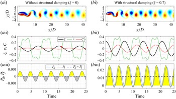
Two cases of rectilinear VIV without SRF, for $m^\star =0.2$
and
$m^\star =0.2$
and $\textit{Re}=100$
, (a) without structural damping (
$\textit{Re}=100$
, (a) without structural damping ( $\xi =0$
) and (b) with structural damping (
$\xi =0$
) and (b) with structural damping ( $\xi =0.7$
): (i) instantaneous iso-contours of spanwise vorticity (
$\xi =0.7$
): (i) instantaneous iso-contours of spanwise vorticity ( $\omega _z\in [-0.75,0.75]$
); (ii) selected time series of the displacement, transverse component of flow velocity and force coefficient; (iii) selected time series of the power associated with energy dissipation by damping and power of fluid forcing, and their time-averaged values. In (i), the rectilinear path is represented by a black dotted line; the sampling point of flow velocity is denoted by a green cross; positive/negative vorticity values are plotted in red/blue. In (ii), the time instant visualised in (i) is indicated by a red dot in the displacement time series. In (iii), the time intervals over which the flow excites/damps body motion, i.e. positive/negative values of the power
$\omega _z\in [-0.75,0.75]$
); (ii) selected time series of the displacement, transverse component of flow velocity and force coefficient; (iii) selected time series of the power associated with energy dissipation by damping and power of fluid forcing, and their time-averaged values. In (i), the rectilinear path is represented by a black dotted line; the sampling point of flow velocity is denoted by a green cross; positive/negative vorticity values are plotted in red/blue. In (ii), the time instant visualised in (i) is indicated by a red dot in the displacement time series. In (iii), the time intervals over which the flow excites/damps body motion, i.e. positive/negative values of the power $P_{\!f}$
, are identified by yellow/grey areas.
$P_{\!f}$
, are identified by yellow/grey areas.

3. Influence of structural damping on VIV
Two cases of rectilinear VIV without SRF are depicted in figure 2, for $m^\star =0.2$
and
$m^\star =0.2$
and $\textit{Re}=100$
, via instantaneous vorticity fields and selected time series of some physical variables. The two cases only differ by the value of the damping ratio,
$\textit{Re}=100$
, via instantaneous vorticity fields and selected time series of some physical variables. The two cases only differ by the value of the damping ratio, $\xi =0$
in (a) versus
$\xi =0$
in (a) versus $\xi =0.7$
in (b). Both cases exhibit a periodic dynamics characterised by flow–body synchronisation (lock-in condition), as illustrated by the time series of the cylinder displacement and transverse component of flow velocity (
$\xi =0.7$
in (b). Both cases exhibit a periodic dynamics characterised by flow–body synchronisation (lock-in condition), as illustrated by the time series of the cylinder displacement and transverse component of flow velocity ( $v$
) sampled
$v$
) sampled $10D$
downstream of the body. The vibrations are close to sinusoidal. These properties are typical of VIV (Williamson & Govardhan Reference Williamson and Govardhan2004), and generally shared by the cases examined in the rest of the paper.
$10D$
downstream of the body. The vibrations are close to sinusoidal. These properties are typical of VIV (Williamson & Govardhan Reference Williamson and Govardhan2004), and generally shared by the cases examined in the rest of the paper.
It appears that the vibration amplitude is much larger in the damped case ( $\zeta _{\textit{max}}=0.25$
) than in the undamped case (
$\zeta _{\textit{max}}=0.25$
) than in the undamped case ( $\zeta _{\textit{max}}=0.09$
). Sustained vibrations imply that, on average, the power associated with energy dissipation by damping,
$\zeta _{\textit{max}}=0.09$
). Sustained vibrations imply that, on average, the power associated with energy dissipation by damping, $P_d=2\pi ^2\textit{St}\xi m^\star \dot \zeta ^2$
(
$P_d=2\pi ^2\textit{St}\xi m^\star \dot \zeta ^2$
( $\textit{St}=0.164$
for
$\textit{St}=0.164$
for $\textit{Re}=100$
), is equal to the power of fluid forcing, i.e.
$\textit{Re}=100$
), is equal to the power of fluid forcing, i.e. $\overline {P_d}=\overline {P_{\!f}}$
;
$\overline {P_d}=\overline {P_{\!f}}$
; $\overline {P_{\!f}}=0$
for
$\overline {P_{\!f}}=0$
for $\xi =0$
. This equilibrium is visualised in figure 2(iii), where the
$\xi =0$
. This equilibrium is visualised in figure 2(iii), where the $P_d$
and
$P_d$
and $P_{\!f}$
time series are plotted together with their time-averaged values. The positive energy transfer from the fluid (
$P_{\!f}$
time series are plotted together with their time-averaged values. The positive energy transfer from the fluid ( $\overline {P_{\!f}}\gt 0$
) is linked to an alteration of the phasing between force and displacement, which are in phase opposition for
$\overline {P_{\!f}}\gt 0$
) is linked to an alteration of the phasing between force and displacement, which are in phase opposition for $\xi =0$
(figure 2ii), as also noted in prior studies on VIV without SRF (e.g. Navrose & Mittal Reference Mittal2017; Bourguet Reference Bourguet2025). These observations show that the level of energy transfer required to compensate the energy dissipated by damping can be attained via an increase in vibration amplitude.
$\xi =0$
(figure 2ii), as also noted in prior studies on VIV without SRF (e.g. Navrose & Mittal Reference Mittal2017; Bourguet Reference Bourguet2025). These observations show that the level of energy transfer required to compensate the energy dissipated by damping can be attained via an increase in vibration amplitude.
Vibration amplitude versus frequency in the rectilinear path configuration without SRF, for $m^\star \in [0.01,3]$
and
$m^\star \in [0.01,3]$
and $\xi \in [0,3]$
(
$\xi \in [0,3]$
( $\textit{Re}=100$
). The symbols are coloured according to the value of the damping ratio in (a) and the energy transferred from the fluid to the structure over one vibration cycle in (b). The iso-contours of
$\textit{Re}=100$
). The symbols are coloured according to the value of the damping ratio in (a) and the energy transferred from the fluid to the structure over one vibration cycle in (b). The iso-contours of $m^\star$
are represented in blue and the values of
$m^\star$
are represented in blue and the values of $m^\star$
are specified in the plots. The Strouhal frequency is indicated by a green dashed line. In (a), black dotted lines visualise the iso-contours of
$m^\star$
are specified in the plots. The Strouhal frequency is indicated by a green dashed line. In (a), black dotted lines visualise the iso-contours of $\xi$
. In (b), the frequency range is normalised by the Strouhal frequency; the free-vibration results are superimposed on the energy map reported by Kumar et al. (Reference Kumar and Mittal2016) on the basis of forced oscillation simulations (adapted with the permission of AIP Publishing); a blue dashed line, obtained by increasing
$\xi$
. In (b), the frequency range is normalised by the Strouhal frequency; the free-vibration results are superimposed on the energy map reported by Kumar et al. (Reference Kumar and Mittal2016) on the basis of forced oscillation simulations (adapted with the permission of AIP Publishing); a blue dashed line, obtained by increasing $\xi$
up to
$\xi$
up to $3000$
, prolongs the
$3000$
, prolongs the $m^\star =0.01$
(
$m^\star =0.01$
( $C_m=-0.01$
) iso-contour down to the low-amplitude region. For
$C_m=-0.01$
) iso-contour down to the low-amplitude region. For $\xi =0$
, the group of large-amplitude responses is identified by grey dashed lines in (a) and cyan dashed lines in (b), while the group of low-amplitude responses is identified by red dashed lines. In both panels, grey squares denote the two cases examined in figure 2.
$\xi =0$
, the group of large-amplitude responses is identified by grey dashed lines in (a) and cyan dashed lines in (b), while the group of low-amplitude responses is identified by red dashed lines. In both panels, grey squares denote the two cases examined in figure 2.

Figure 3. Long description
Panel A: A scatter plot shows the relationship between vibration amplitude and frequency. The x-axis represents frequency, and the y-axis represents maximum vibration amplitude. Symbols are colored according to the value of the damping ratio. Black dotted lines visualize the iso-contours of a specific parameter. Panel B: A contour plot overlays a scatter plot, showing the energy transferred from the fluid to the structure over one vibration cycle. The x-axis represents the frequency normalized by the Strouhal frequency, and the y-axis represents maximum vibration amplitude. Iso-contours of another parameter are represented in blue. The Strouhal frequency is indicated by a green dashed line. A blue dashed line prolongs a specific iso-contour down to the low-amplitude region. Grey squares denote two specific cases examined in another figure.
To investigate the possible amplification of VIV by damping in the above configuration, the evolution of the structural response for $m^\star \in [0.01,3]$
and
$m^\star \in [0.01,3]$
and $\xi \in [0,3]$
is represented in figure 3, in the amplitude–frequency domain; the vibration frequency (
$\xi \in [0,3]$
is represented in figure 3, in the amplitude–frequency domain; the vibration frequency ( $f_\zeta$
) is normalised by St in (b). The symbols are coloured by
$f_\zeta$
) is normalised by St in (b). The symbols are coloured by $\xi$
value in (a) and by the value of the energy transferred from the fluid to the structure over one vibration cycle,
$\xi$
value in (a) and by the value of the energy transferred from the fluid to the structure over one vibration cycle, $E=\overline {P_{\!f}}/f_\zeta$
, in (b). For
$E=\overline {P_{\!f}}/f_\zeta$
, in (b). For $\xi =0$
, two groups or branches of responses, indicated by dashed lines in figure 3, can be identified: a group of large-amplitude responses in the lower-
$\xi =0$
, two groups or branches of responses, indicated by dashed lines in figure 3, can be identified: a group of large-amplitude responses in the lower- $m^\star$
range, with amplitudes close to
$m^\star$
range, with amplitudes close to $0.4D$
, and a group characterised by lower amplitudes, of the order of
$0.4D$
, and a group characterised by lower amplitudes, of the order of $0.1D$
, for higher
$0.1D$
, for higher $m^\star$
. The abrupt reduction in vibration amplitude observed between
$m^\star$
. The abrupt reduction in vibration amplitude observed between $m^\star =0.1$
and
$m^\star =0.1$
and $m^\star =0.2$
was associated with the concept of ‘critical mass ratio’ in prior works (e.g. Govardhan & Williamson Reference Govardhan and Williamson2002). As shown in figure 3(b), the undamped responses, for which
$m^\star =0.2$
was associated with the concept of ‘critical mass ratio’ in prior works (e.g. Govardhan & Williamson Reference Govardhan and Williamson2002). As shown in figure 3(b), the undamped responses, for which $E=0$
, occur along the
$E=0$
, occur along the $E=0$
iso-contour, or in the region of low
$E=0$
iso-contour, or in the region of low $E$
, determined via forced sinusoidal oscillations by Kumar et al. (Reference Kumar and Mittal2016); some deviations are expected as the present responses are not strictly sinusoidal and may appear close to the edge of the region of flow–body synchronisation captured by the forced oscillations.
$E$
, determined via forced sinusoidal oscillations by Kumar et al. (Reference Kumar and Mittal2016); some deviations are expected as the present responses are not strictly sinusoidal and may appear close to the edge of the region of flow–body synchronisation captured by the forced oscillations.
The two groups of undamped responses exhibit different trends when structural damping is introduced. In the lower- $m^\star$
group, where the large-amplitude responses are concentrated, the amplitude decreases monotonically as
$m^\star$
group, where the large-amplitude responses are concentrated, the amplitude decreases monotonically as $\xi$
is increased. This trend corresponds to the typical effect of damping on VIV reported in previous studies (e.g. Klamo et al. Reference Klamo, Leonard and Roshko2006). In contrast, in the higher-
$\xi$
is increased. This trend corresponds to the typical effect of damping on VIV reported in previous studies (e.g. Klamo et al. Reference Klamo, Leonard and Roshko2006). In contrast, in the higher- $m^\star$
group, the amplitude first increases with
$m^\star$
group, the amplitude first increases with $\xi$
, before reaching a peak value and then decreasing. The amplification due to damping can be substantial, especially close to the transition between the two response groups, as illustrated by the cases examined in figure 2 (grey squares in figure 3). Regardless of the evolution of the amplitude, the vibration frequency globally increases with
$\xi$
, before reaching a peak value and then decreasing. The amplification due to damping can be substantial, especially close to the transition between the two response groups, as illustrated by the cases examined in figure 2 (grey squares in figure 3). Regardless of the evolution of the amplitude, the vibration frequency globally increases with $\xi$
, and tends towards
$\xi$
, and tends towards $St$
(green dashed lines).
$St$
(green dashed lines).
(a) Vibration amplitude, (b) vibration frequency and (c) damping ratio associated with the peak amplitude and amplification factor, as functions of the mass ratio, in the rectilinear path configuration without SRF, for (i) $\textit{Re}=100$
, (ii)
$\textit{Re}=100$
, (ii) $\textit{Re}=160$
and (iii)
$\textit{Re}=160$
and (iii) $\textit{Re}=40$
. In (a,b), three values of the damping ratio are considered,
$\textit{Re}=40$
. In (a,b), three values of the damping ratio are considered, $\xi \in \{0,0.1,0.5\}$
. In (a), the peak amplitude attained by varying the damping ratio, i.e. for
$\xi \in \{0,0.1,0.5\}$
. In (a), the peak amplitude attained by varying the damping ratio, i.e. for $\xi =\xi _{\textit{peak}}$
, is represented by a grey dotted line. In (b), a green dashed line indicates the Strouhal frequency. Yellow and grey background colours identify the
$\xi =\xi _{\textit{peak}}$
, is represented by a grey dotted line. In (b), a green dashed line indicates the Strouhal frequency. Yellow and grey background colours identify the $m^\star$
ranges where the peak amplitude is reached for
$m^\star$
ranges where the peak amplitude is reached for $\xi \gt 0$
and
$\xi \gt 0$
and $\xi =0$
, respectively. In (iii), horizontal stripes denote the
$\xi =0$
, respectively. In (iii), horizontal stripes denote the $m^\star$
range where vibrations do not develop without damping but arise beyond a threshold value of
$m^\star$
range where vibrations do not develop without damping but arise beyond a threshold value of $\xi$
; the amplification factor is not defined in this interval.
$\xi$
; the amplification factor is not defined in this interval.

Without SRF, the mass ratio is equal to the opposite of the added mass coefficient, $C_m=-2\overline {C\ddot \zeta }/(\pi \overline {\ddot \zeta ^2})=-m^\star$
. Therefore, each iso-contour of
$C_m=-2\overline {C\ddot \zeta }/(\pi \overline {\ddot \zeta ^2})=-m^\star$
. Therefore, each iso-contour of $m^\star$
visited when
$m^\star$
visited when $\xi$
is varied (blue lines), i.e. the possible states of the system for a given
$\xi$
is varied (blue lines), i.e. the possible states of the system for a given $m^\star$
, represents an iso-contour of
$m^\star$
, represents an iso-contour of $C_m$
. This explains why the iso-contours of
$C_m$
. This explains why the iso-contours of $m^\star$
do not intersect. For the lowest
$m^\star$
do not intersect. For the lowest $m^\star$
value under study (
$m^\star$
value under study ( $0.01$
),
$0.01$
), $\xi$
is increased to
$\xi$
is increased to $3000$
to trace the iso-contour down to low amplitudes, and delimit the region of the amplitude–frequency domain accessible without SRF (blue dotted line in figure 3
b); the maximum level of energy transfer,
$3000$
to trace the iso-contour down to low amplitudes, and delimit the region of the amplitude–frequency domain accessible without SRF (blue dotted line in figure 3
b); the maximum level of energy transfer, $E=0.23$
(
$E=0.23$
( $\overline {P_{\!f}}=\overline {P_d}=0.037$
), is reached for
$\overline {P_{\!f}}=\overline {P_d}=0.037$
), is reached for $\xi =42$
. The values of
$\xi =42$
. The values of $E$
along the iso-contours of
$E$
along the iso-contours of $m^\star$
(and
$m^\star$
(and $C_m$
) match the forced oscillation results (figure 3
b), which can be used to visualise the global distribution of
$C_m$
) match the forced oscillation results (figure 3
b), which can be used to visualise the global distribution of $E$
and interpret the above contrasting trends. The shape of these iso-contours relative to the distribution of
$E$
and interpret the above contrasting trends. The shape of these iso-contours relative to the distribution of $E$
determines whether a variation of
$E$
determines whether a variation of $\xi$
, and thus a new level of energy transfer required to balance the dissipation by damping, will amplify or attenuate the vibration. The curved shape of the iso-contours near the amplitude drop, close to
$\xi$
, and thus a new level of energy transfer required to balance the dissipation by damping, will amplify or attenuate the vibration. The curved shape of the iso-contours near the amplitude drop, close to $m^\star = 0.2$
, with a large vertical excursion, results in a pronounced amplification by damping in this
$m^\star = 0.2$
, with a large vertical excursion, results in a pronounced amplification by damping in this $m^\star$
range. The phenomenon tends to be less prominent for higher
$m^\star$
range. The phenomenon tends to be less prominent for higher $m^\star$
values, due to the more horizontal shape and smaller vertical excursion of the iso-contours.
$m^\star$
values, due to the more horizontal shape and smaller vertical excursion of the iso-contours.
The vibration amplitude and frequency for $\xi \in \{0,0.1,0.5\}$
are plotted as functions of
$\xi \in \{0,0.1,0.5\}$
are plotted as functions of $m^\star$
in figure 4(a,b), for
$m^\star$
in figure 4(a,b), for $\textit{Re}=100$
(the Re value considered above),
$\textit{Re}=100$
(the Re value considered above), $\textit{Re}=160$
and
$\textit{Re}=160$
and $\textit{Re}=40$
;
$\textit{Re}=40$
; ${ St}=0.185$
for
${ St}=0.185$
for $\textit{Re}=160$
, and for
$\textit{Re}=160$
, and for $\textit{Re}=40$
, the St value (
$\textit{Re}=40$
, the St value ( $0.115$
) is that obtained by Kou et al. (Reference Kou, Zhang, Liu and Li2017) by triggering the flow. The peak amplitude attained when
$0.115$
) is that obtained by Kou et al. (Reference Kou, Zhang, Liu and Li2017) by triggering the flow. The peak amplitude attained when $\xi$
is varied is also plotted in figure 4(a). The corresponding value of the damping ratio,
$\xi$
is varied is also plotted in figure 4(a). The corresponding value of the damping ratio, $\xi _{\textit{peak}}=\textrm {argmax}_{\xi \geqslant 0} (\zeta _{\textit{max}}(\xi ) )$
, and the amplification factor relative to the undamped case,
$\xi _{\textit{peak}}=\textrm {argmax}_{\xi \geqslant 0} (\zeta _{\textit{max}}(\xi ) )$
, and the amplification factor relative to the undamped case, $A_\zeta =[{\zeta _{\textit{max}}(\xi =\xi _{\textit{peak}})-\zeta _{\textit{max}}(\xi =0)}]/{\zeta _{\textit{max}}(\xi =0)}$
, are presented in figure 4(c).
$A_\zeta =[{\zeta _{\textit{max}}(\xi =\xi _{\textit{peak}})-\zeta _{\textit{max}}(\xi =0)}]/{\zeta _{\textit{max}}(\xi =0)}$
, are presented in figure 4(c).
The amplifying effect of damping beyond a threshold value of $m^\star$
, identified above for
$m^\star$
, identified above for $\textit{Re}=100$
, is found to persist for the two other
$\textit{Re}=100$
, is found to persist for the two other $\textit{Re}$
values. The
$\textit{Re}$
values. The $m^\star$
range where
$m^\star$
range where $A_\zeta \gt 0$
is indicated by a yellow background colour. For
$A_\zeta \gt 0$
is indicated by a yellow background colour. For $\textit{Re}=160$
, the amplification exceeds
$\textit{Re}=160$
, the amplification exceeds $200\,\%$
. In the subcritical-
$200\,\%$
. In the subcritical- $\textit{Re}$
case (
$\textit{Re}$
case ( $\textit{Re}=40$
), vibrations cease beyond
$\textit{Re}=40$
), vibrations cease beyond $m^\star =0.75$
for
$m^\star =0.75$
for $\xi =0$
, but can occur up to
$\xi =0$
, but can occur up to $m^\star =1.75$
for
$m^\star =1.75$
for $\xi \gt 0$
(striped area in figure 4iii). As a result, structural damping not only amplifies VIV, but also causes vibrations and flow unsteadiness to develop in conditions where the undamped system remains steady.
$\xi \gt 0$
(striped area in figure 4iii). As a result, structural damping not only amplifies VIV, but also causes vibrations and flow unsteadiness to develop in conditions where the undamped system remains steady.
(a) Vibration amplitude without damping, (b) peak amplitude reached when $\xi$
is varied, (c) damping ratio associated with the peak amplitude and (d) amplification factor, as functions of the Reynolds number and mass ratio, in the rectilinear path configuration without SRF. A white solid line delimits the vibration region for
$\xi$
is varied, (c) damping ratio associated with the peak amplitude and (d) amplification factor, as functions of the Reynolds number and mass ratio, in the rectilinear path configuration without SRF. A white solid line delimits the vibration region for $\xi =0$
in (a), and for
$\xi =0$
in (a), and for $\xi =\xi _{\textit{peak}}$
in (b–d); in (b–d), the limit of the vibration region for
$\xi =\xi _{\textit{peak}}$
in (b–d); in (b–d), the limit of the vibration region for $\xi =0$
is indicated by a white dotted line. The region where damping systematically reduces vibration amplitude (
$\xi =0$
is indicated by a white dotted line. The region where damping systematically reduces vibration amplitude ( $\xi _{\textit{peak}}=0$
,
$\xi _{\textit{peak}}=0$
, $A_\zeta =0$
) is delineated by a white dashed line. A blue dashed–dotted line denotes the critical
$A_\zeta =0$
) is delineated by a white dashed line. A blue dashed–dotted line denotes the critical $\textit{Re}$
for the onset of flow unsteadiness for a fixed cylinder. The regions where
$\textit{Re}$
for the onset of flow unsteadiness for a fixed cylinder. The regions where $\xi _{\textit{peak}}$
and
$\xi _{\textit{peak}}$
and $A_\zeta$
are not defined are masked. In (a), a green cross and green dotted lines locate the cases examined in figures 2 and 4.
$A_\zeta$
are not defined are masked. In (a), a green cross and green dotted lines locate the cases examined in figures 2 and 4.

Figure 5. Long description
Panel A: A heat map shows the vibration amplitude without damping as a function of the Reynolds number (Re) and mass ratio (m*). The color scale ranges from black to white, indicating increasing amplitude values. A white solid line delineates the vibration region. A green cross and dotted lines mark specific cases examined in other figures. Panel B: Another heat map displays the peak amplitude reached when a parameter is varied, with a similar color scale. A white solid line and a white dotted line indicate the vibration regions for different parameters. A blue dashed-dotted line denotes the critical Re for flow unsteadiness onset. Panel C: A heat map illustrates the damping ratio associated with the peak amplitude, using a color scale from black to yellow. The white solid and dotted lines, and the blue dashed-dotted line are also present. Panel D: The final heat map shows the amplification factor, with a color scale from black to yellow. The same lines and regions as in the previous panels are included.
A continuous vision of the effect of structural damping is proposed in figure 5, which represents the vibration amplitudes for $\xi =0$
and
$\xi =0$
and $\xi =\xi _{\textit{peak}}$
, as well as
$\xi =\xi _{\textit{peak}}$
, as well as $\xi _{\textit{peak}}$
and
$\xi _{\textit{peak}}$
and $A_\zeta$
, in the
$A_\zeta$
, in the $(\textit{Re},m^\star )$
domain. The lowest
$(\textit{Re},m^\star )$
domain. The lowest $\textit{Re}$
value where VIV appear for the undamped system, close to
$\textit{Re}$
value where VIV appear for the undamped system, close to $30$
for
$30$
for $m^\star =0.01$
, is not reduced as
$m^\star =0.01$
, is not reduced as $\xi$
is increased. However, for slightly higher
$\xi$
is increased. However, for slightly higher $m^\star$
, structural damping induces an extension of the vibration region, delimited by a white solid line, towards lower subcritical values of
$m^\star$
, structural damping induces an extension of the vibration region, delimited by a white solid line, towards lower subcritical values of $\textit{Re}$
; the critical threshold
$\textit{Re}$
; the critical threshold $\textit{Re}=47$
is indicated by a blue dashed–dotted line. This extension is illustrated in figure 4(iii). The area where damping systematically attenuates VIV (
$\textit{Re}=47$
is indicated by a blue dashed–dotted line. This extension is illustrated in figure 4(iii). The area where damping systematically attenuates VIV ( $\xi _{\textit{peak}}=0$
,
$\xi _{\textit{peak}}=0$
, $A_\zeta =0$
), in the lower-
$A_\zeta =0$
), in the lower- $m^\star$
range, is delineated by a white dashed line in figure 5. In the rest of the vibration region, damping can amplify VIV. The amplification is particularly pronounced near the limit of the
$m^\star$
range, is delineated by a white dashed line in figure 5. In the rest of the vibration region, damping can amplify VIV. The amplification is particularly pronounced near the limit of the $m^\star$
range where
$m^\star$
range where $A_\zeta \gt 0$
, beyond
$A_\zeta \gt 0$
, beyond $\textit{Re}=80$
. It tends to smooth the amplitude drop observed without damping. The largest values of
$\textit{Re}=80$
. It tends to smooth the amplitude drop observed without damping. The largest values of $A_\zeta$
are reached for relatively high damping ratios, ranging from
$A_\zeta$
are reached for relatively high damping ratios, ranging from $0.5$
to
$0.5$
to $1$
approximately.
$1$
approximately.
The distributions of energy transfer in the amplitude–frequency domain, obtained via forced oscillation experiments for higher Re (e.g. Hover et al. Reference Hover, Techet and Triantafyllou1998; Morse & Williamson Reference Morse and Williamson2009), resemble the distribution depicted in figure 3(b). This similarity suggests that amplification by damping could also occur for higher Re. As a first exploratory step in this direction, preliminary simulations for $\textit{Re}=250$
(not presented) indicate that the phenomenon persists when the flow undergoes three-dimensional transition.
$\textit{Re}=250$
(not presented) indicate that the phenomenon persists when the flow undergoes three-dimensional transition.
Same as figure 4, for $\textit{Re}=100$
: (i,ii) curvilinear path configuration without SRF, for (i)
$\textit{Re}=100$
: (i,ii) curvilinear path configuration without SRF, for (i) $\kappa =1$
and (ii)
$\kappa =1$
and (ii) $\kappa =5$
; (iii,iv) rectilinear path configuration with SRF, for (iii)
$\kappa =5$
; (iii,iv) rectilinear path configuration with SRF, for (iii) $m^\star =1$
and (iv)
$m^\star =1$
and (iv) $m^\star =0.3$
. In (ii), the
$m^\star =0.3$
. In (ii), the $m^\star$
axis range is discontinuous. In (iii,iv), the results are plotted as functions of the reduced velocity.
$m^\star$
axis range is discontinuous. In (iii,iv), the results are plotted as functions of the reduced velocity.

The above results show that the rectilinear VIV developing in the lower- $m^\star$
range are always attenuated by structural damping, and that the amplifying effect of damping only arises beyond a threshold value of
$m^\star$
range are always attenuated by structural damping, and that the amplifying effect of damping only arises beyond a threshold value of $m^\star$
. As reported in prior works concerning undamped VIV without SRF (Bourguet Reference Bourguet2023, Reference Bourguet2024), path curvature tends to displace the large-amplitude responses towards lower
$m^\star$
. As reported in prior works concerning undamped VIV without SRF (Bourguet Reference Bourguet2023, Reference Bourguet2024), path curvature tends to displace the large-amplitude responses towards lower $C_m$
, and thus larger
$C_m$
, and thus larger $m^\star$
values. Beyond a certain curvature, close to
$m^\star$
values. Beyond a certain curvature, close to $3.5$
for
$3.5$
for $\textit{Re}=100$
, a branch of low-amplitude responses, comparable to those enhanced by damping in the rectilinear path configuration, emerges near
$\textit{Re}=100$
, a branch of low-amplitude responses, comparable to those enhanced by damping in the rectilinear path configuration, emerges near $m^\star =0$
. The effect of structural damping along curved trajectories (configuration schematised in figure 1
b) is examined in figure 6(i,ii), for
$m^\star =0$
. The effect of structural damping along curved trajectories (configuration schematised in figure 1
b) is examined in figure 6(i,ii), for $\kappa =1$
and
$\kappa =1$
and $\kappa =5$
(
$\kappa =5$
( $\textit{Re}=100$
), adopting the same presentation as in figure 4. It can be noted that the amplifying effect of damping also exists for curvilinear vibrations (yellow areas where
$\textit{Re}=100$
), adopting the same presentation as in figure 4. It can be noted that the amplifying effect of damping also exists for curvilinear vibrations (yellow areas where $A_\zeta \gt 0$
), even though the amplification appears to be less pronounced than for rectilinear VIV. In addition, as conjectured from prior results, the low-amplitude responses occurring in the lower-
$A_\zeta \gt 0$
), even though the amplification appears to be less pronounced than for rectilinear VIV. In addition, as conjectured from prior results, the low-amplitude responses occurring in the lower- $m^\star$
range for
$m^\star$
range for $\kappa =5$
can be amplified by damping. As a consequence, depending on path curvature, the amplifying effect of structural damping can be observed for any
$\kappa =5$
can be amplified by damping. As a consequence, depending on path curvature, the amplifying effect of structural damping can be observed for any $m^\star$
, including values close to
$m^\star$
, including values close to $m^\star =0$
.
$m^\star =0$
.
Previous studies concerning undamped rectilinear VIV with SRF suggest that low-amplitude responses susceptible to significant amplification by damping could appear for $m^\star$
values of the order of
$m^\star$
values of the order of $1$
or lower (Navrose & Mittal Reference Mittal2017; Bourguet Reference Bourguet2025). This is indeed the case, as illustrated in figure 6(iii,iv), where the influence of damping on rectilinear vibrations is visualised, over a range of reduced velocities, for
$1$
or lower (Navrose & Mittal Reference Mittal2017; Bourguet Reference Bourguet2025). This is indeed the case, as illustrated in figure 6(iii,iv), where the influence of damping on rectilinear vibrations is visualised, over a range of reduced velocities, for $m^\star =1$
and
$m^\star =1$
and $m^\star =0.3$
(configuration schematised in figure 1
c;
$m^\star =0.3$
(configuration schematised in figure 1
c; $\textit{Re}=100$
). The amplification levels are comparable to those attained without SRF. Additional simulations (not presented) show that an amplification of VIV by damping can also be observed when the cylinder is elastically mounted in both the cross-flow and streamwise directions, i.e. with two degrees of freedom.
$\textit{Re}=100$
). The amplification levels are comparable to those attained without SRF. Additional simulations (not presented) show that an amplification of VIV by damping can also be observed when the cylinder is elastically mounted in both the cross-flow and streamwise directions, i.e. with two degrees of freedom.
Considering the generality of the amplifying effect of structural damping, the question that naturally arises is why this phenomenon has not been previously documented. Two explanations can be proposed. First, the amplifying effect of damping affects low-amplitude response branches, while prior works focused on the peak-amplitude responses, which tend to be systematically attenuated when $\xi$
is increased. Second, the majority of studies on damping effects were carried out with SRF and relatively large values of
$\xi$
is increased. Second, the majority of studies on damping effects were carried out with SRF and relatively large values of $m^\star$
, compared with the range in which the amplification due to damping becomes particularly significant. It can be mentioned that this range of
$m^\star$
, compared with the range in which the amplification due to damping becomes particularly significant. It can be mentioned that this range of $m^\star$
corresponds to typical values encountered in ocean engineering applications, i.e. of the order of unity. Amplification by damping is expected to occur for high Re, and the reported amplification levels may have a dramatic influence on the fatigue life of risers and offshore structures exposed to ocean currents. This phenomenon should therefore be taken into account in fatigue damage prediction models. The possible amplification of VIV by damping should also be considered in the development of flow energy harvesting systems, especially small-scale devices which can operate in the
$m^\star$
corresponds to typical values encountered in ocean engineering applications, i.e. of the order of unity. Amplification by damping is expected to occur for high Re, and the reported amplification levels may have a dramatic influence on the fatigue life of risers and offshore structures exposed to ocean currents. This phenomenon should therefore be taken into account in fatigue damage prediction models. The possible amplification of VIV by damping should also be considered in the development of flow energy harvesting systems, especially small-scale devices which can operate in the $\textit{Re}$
range examined in this work.
$\textit{Re}$
range examined in this work.
4. Conclusions
The influence of structural damping on VIV has been investigated numerically, for different variants of the canonical problem commonly used to study this form of flow-induced vibrations, i.e. a circular cylinder free to oscillate within a uniform cross-current, over a range of $\textit{Re}$
values up to
$\textit{Re}$
values up to $160$
.
$160$
.
As a first step, focus was placed on rectilinear VIV without SRF. In the absence of structural damping, the peak-amplitude responses are concentrated in the lower- $m^\star$
range. These peak-amplitude responses are consistently attenuated by an increase in
$m^\star$
range. These peak-amplitude responses are consistently attenuated by an increase in $\xi$
, in agreement with prior works. A contrasting trend arises for the lower-amplitude responses occurring for higher
$\xi$
, in agreement with prior works. A contrasting trend arises for the lower-amplitude responses occurring for higher $m^\star$
: the vibrations can be amplified as
$m^\star$
: the vibrations can be amplified as $\xi$
increases. This phenomenon is observed over the entire range of
$\xi$
increases. This phenomenon is observed over the entire range of $\textit{Re}$
under study. The evolution of VIV amplitude with
$\textit{Re}$
under study. The evolution of VIV amplitude with $\xi$
has been analysed in relation to the distribution of fluid–structure energy transfer in the amplitude–frequency domain.
$\xi$
has been analysed in relation to the distribution of fluid–structure energy transfer in the amplitude–frequency domain.
The amplification induced by damping is particularly pronounced near the limit of the $m^\star$
interval where the phenomenon appears, for damping ratios ranging from
$m^\star$
interval where the phenomenon appears, for damping ratios ranging from $0.5$
to
$0.5$
to $1$
. The amplification exceeds
$1$
. The amplification exceeds $200\,\%$
relative to the amplitudes measured for
$200\,\%$
relative to the amplitudes measured for $\xi =0$
, leading to vibrations that become significant compared with the peak-amplitude responses. Structural damping amplifies VIV, but also causes vibrations and flow unsteadiness to develop for subcritical values of
$\xi =0$
, leading to vibrations that become significant compared with the peak-amplitude responses. Structural damping amplifies VIV, but also causes vibrations and flow unsteadiness to develop for subcritical values of $\textit{Re}$
where the undamped system remains steady; in other words, damping extends the subcritical-
$\textit{Re}$
where the undamped system remains steady; in other words, damping extends the subcritical- $\textit{Re}$
range of VIV.
$\textit{Re}$
range of VIV.
The enhancement of VIV by structural damping is a counterintuitive but general phenomenon. This effect persists along curvilinear paths. Depending on path curvature, amplification can occur for any $m^\star$
, including values close to
$m^\star$
, including values close to $m^\star =0$
, where rectilinear VIV are attenuated by an increase in
$m^\star =0$
, where rectilinear VIV are attenuated by an increase in $\xi$
. Furthermore, amplification levels comparable to those attained without SRF can be reached with SRF.
$\xi$
. Furthermore, amplification levels comparable to those attained without SRF can be reached with SRF.
Acknowledgements
This work was performed using HPC resources from CALMIP (P1248-2025,2026).
Declaration of interests
The author reports no conflict of interest.

 m⋆=0.2
 Re=100
 ξ=0
ξ=0 ξ=0.7
ξ=0.7 ωz∈[−0.75,0.75]
 Pf
Pf
 m⋆∈[0.01,3]
 ξ∈[0,3]
 Re=100
 m⋆
m⋆ m⋆
m⋆ ξ
ξ ξ
ξ 3000
3000 m⋆=0.01
 Cm=−0.01
 ξ=0
ξ=0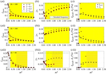
 Re=100
 Re=160
 Re=40
Re=40 ξ∈{0,0.1,0.5}
 ξ=ξpeak
 m⋆
m⋆ ξ>0
ξ>0 ξ=0
ξ=0 m⋆
m⋆ ξ
ξ
 ξ
ξ ξ=0
ξ=0 ξ=ξpeak
 ξ=0
ξ=0 ξpeak=0
 Aζ=0
Aζ=0 Re
Re ξpeak
ξpeak Aζ
Aζ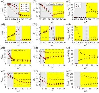
 Re=100
 κ=1
κ=1 κ=5
κ=5 m⋆=1
m⋆=1 m⋆=0.3
 m⋆
m⋆
 Open access

