3.1. Impact of two droplets: lamella spreading dynamics and central sheet formation

This section provides a comparison between the dynamics of two-droplet impacts (with dimensionless inter-droplet spacing $\Delta x^{*}=\Delta x/D_0=1.80$) and an equivalent single-droplet impact case ($We\approx 80$, $Re\approx 3750$, $D_{0}=3.12\pm 0.02$). This allows establishing, initially qualitatively, the way that the dynamics change during the simultaneous two droplet impacts. The single-droplet impact was accomplished by masking one of the needles of the droplet-pair generator to allow the delivery of a single droplet. Figure 3(a) presents a selection of front-view images at different dimensionless times ($\tau \approx 0-20$) of the impact of the single droplet and the droplet pair (see also supplementary movie 1 available at https://doi.org/10.1017/jfm.2023.249). Upon impact, the liquid lamella that emerges underneath each droplet starts to spread radially outwards on the surface, with a continuous decrease in the impacting droplet height. The spreading of the lamella on the surface is characterised by an instantaneous spread radius, $R(t)$, which is defined in figure 3(b) for both impact processes.

Figure 3.

Surface impact process for a single droplet and a droplet pair on a solid surface ($We =80$ for both cases, and $\Delta x^* =1.80$ for the droplet pair). (a) Front-view images of the temporal evolution of the impact processes. Scale bars are 2 mm. (b) Schematic of the calculation of spread radius ($R(t)$) from the impact centre of a droplet for both cases. (c) Dimensionless spread radius ($R^*=R/D_0$) as a function of dimensionless time ($\tau = tV_0/D_0$) for both cases, in comparison to the theory of (1) Roisman et al. (Reference Roisman, Prunet-Foch, Tropea and Vignes-Adler2002), (2) Gordillo, Riboux & Quintero (Reference Gordillo, Riboux and Quintero2019) and (3) the empirical model by Lejeune, Gilet & Bourouiba (Reference Lejeune, Gilet and Bourouiba2018). See supplementary movie 1 for the corresponding video.

For the single-droplet impact with $We\approx 80$ (figure 3a), the rim-bounded spreading lamella reaches a maximum spread radius ($R_{max}$) at $\tau \approx 2.25$. At $R_{max}$, the contact line remains stationary while a receding contact angle is achieved at the lamella periphery, and subsequently, the liquid contact retracts back towards the impact centre. This receding liquid eventually deposits on the surface with an equilibrium shape at $\tau >20$ (see supplementary movie 1). However, for the droplet-pair impact with $\Delta x^*=1.80$ and $We\approx 80$ (figure 3a), the individual spreading lamellae start interacting with each other at the initial stage of their spreading ($\tau \approx 0.4$). Due to the high kinetic energy of the lamellae, their interaction generates an uprising liquid sheet along the line of intersection. During this stage, stagnation points form on the surface at the intersection line, and the interacting liquid flows are redirected laterally and vertically on the impact surface (Batzdorf et al. Reference Batzdorf, Breitenbach, Schlawitschek, Roisman, Tropea, Stephan and Gambaryan-Roisman2017; Gultekin et al. Reference Gultekin, Erkan, Ozdemir, Colak and Suzuki2021). The central uprising sheet grows rapidly, reaches a summit ($\tau \approx 2.25$), and falls back on the liquid mass underneath due to surface tension and gravity ($\tau \approx 5.5$). The surface liquid also recedes, similar to the single-droplet case, and finally attains an equilibrium shape after $\tau \approx 20$. For the single- and droplet-pair cases, the final equilibrium shape resembles a single sessile drop (see supplementary movie 1). The images of figure 3(a) indicate that the spreading of the non-interacting lamella segments remains unaffected on the impact surface during the formation and growth of the central uprising sheet. Roisman et al. (Reference Roisman, Prunet-Foch, Tropea and Vignes-Adler2002) also demonstrated similar spreading behaviour using the top-view images of droplet-pair impacts.

For the isolated and non-isolated impact cases of figure 3(a), we applied an image analysis algorithm that determines the impact centre of a droplet and measures the instantaneous spread radius ($R(t)$), as defined in figure 3(b). The temporal evolution of the dimensionless spread radius ($R^*(\tau )=R(t)/D_0$) for single-droplet and droplet-pair impacts up to $\tau \approx 3.0$ is shown in figure 3(c). For the isolated single droplet, $R^*$ of the advancing lamella reaches a maximum value, which is approximately 1.65 times the initial droplet diameter ($D_0$) at $\tau \approx 2.25$ and then $R^*$ decreases as the lamella recedes. For the non-isolated droplets of the droplet pair, $R^*$ was measured from $\tau =\tau _0\approx 0.4$, where $\tau _0$ is the instant of the initiation of lamella interaction. The temporal evolution of $R^*$ of the non-isolated droplets superposes on that of the isolated single droplet, with a negligible relative difference (maximum of 1.7 %), see figure 3(c). This superposition corroborates the idea that, for the droplet-pair impact, the portion of the liquid lamella that does not contribute to the central sheet formation spreads on the dry substrate, remaining unaffected by the ascending central sheet.

Numerous theoretical relations exist to estimate the maximum spread radius ($R_{max}$) on dry solid substrates in terms of different dimensionless parameters, which are individually a function of the impact parameters (Josserand & Thoroddsen Reference Josserand and Thoroddsen2016). However, such theoretical relations for the time-dependent spread radius, $R(t)$, are far less reported in the literature (Yarin et al. Reference Yarin2006). An earlier study of Roisman et al. (Reference Roisman, Prunet-Foch, Tropea and Vignes-Adler2002) considered the mass and momentum balance equations of a lamella rim to develop an analytical model, which allows estimating $R(t)$ in a dimensionless form as

(3.1)\begin{equation} R^{{\ast}}\left(\tau\right)=A\left(\tau+\omega\right)-B\left(\tau+\omega\right)^2, \end{equation}

where $A$, $B$ and $\omega$ are three dimensionless parameters which depend on the Weber number $We$, the Reynolds number $Re$ and the static advancing contact angle $\theta _{A}$ (see Roisman et al. (Reference Roisman, Prunet-Foch, Tropea and Vignes-Adler2002) for related details). It is noted that (3.1) was developed for $1 \leq \tau \leq \tau _{max }$, where $\tau _{max}$ is the dimensionless time that corresponds to the dimensionless maximum spread radius ($R_{max}^*$). Using the experimental parameters of the impact processes of figure 3(a), we obtain $A\approx 1.48$, $B\approx 0.32$ and $\omega \approx 0.27$. The prediction of (3.1) is compared to the current measurements in figure 3(c), where the theoretical line is extended for $\tau <1$ and slightly for $\tau >\tau _{max}$. Although (3.1) predicts the time for $R_{max}^*$ approximately in agreement with that for the measured $R_{max}^*$ (i.e. $\tau _{max}\approx 2.25$), it overestimates $R_{max}^*$ with a relative mean error of $\approx 11.84\,\%$. Other authors also find similar divergence, e.g. a relative mean error of $11.64\pm 5.94\,\%$ (Ukiwe & Kwok Reference Ukiwe and Kwok2005) and $14.17\pm 1.88\,\%$ (Ukiwe, Mansouri & Kwok Reference Ukiwe, Mansouri and Kwok2005), while comparing their measured $R_{max}^*$ to the prediction of (3.1). The limitation of this theoretical model lies primarily in the fact that the authors approximated the droplet shape as a circular disc of constant thickness from $\tau =1$, which is ‘not correct’ as mentioned in a later study (Roisman, Berberović & Tropea Reference Roisman, Berberović and Tropea2009). Figure 3(a) also reveals, for both single and droplet pair cases, that the disk shape is not flat at $\tau =1$, but becomes flat at $\tau \approx 2$. In addition, the contact line velocity of the spreading lamella is equated to the impact velocity ($V_0$) in this theory, whereas the contact line velocity of a spreading lamella is several times larger than the droplet impact velocity (Ukiwe & Kwok Reference Ukiwe and Kwok2005). The temporal evolution of the velocity of the lamella contact lines and that of the central uprising sheet is detailed in Appendix A. Considering more realistic hypotheses and by applying mass and momentum balances at the lamella rim, Gordillo et al. (Reference Gordillo, Riboux and Quintero2019) deduced a set of ordinary differential equations that govern the time-dependent spread radius $R^* (\tau )$. We numerically solved their equations using MATLAB for our experimental conditions, and figure 3(c) also presents the obtained droplet spreading radius $R^*(\tau )$ (for a hydrophilic surface and in our dimensionless form), which is in excellent agreement with our measurements. Recently, Gorin et al. (Reference Gorin, Di Mauro, Bonn and Kellay2022) also observed similar agreement with the theory of Gordillo et al. (Reference Gordillo, Riboux and Quintero2019) for both Newtonian and non-Newtonian droplet impacts. Figure 3(c) also presents $R^*(\tau )$ from the empirical model of Lejeune et al. (Reference Lejeune, Gilet and Bourouiba2018) and shows a reasonably good agreement with our measurements.

3.2. Morphology of the central sheet evolution

3.2.1. Effect of impact Weber number

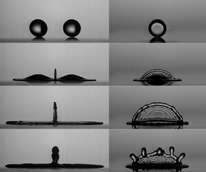
Figures 4 and 5 respectively show a series of front-view and side-view images of the simultaneous impacts of two droplets at different dimensionless times for four different impact Weber numbers ($We$) with a fixed inter-droplet spacing of $\Delta x^{\ast }=1.80\pm 0.03$ (see also supplementary movies 2–5). These images reveal the morphology of the central sheet evolution in vertical and lateral directions. For all cases, the kinetic energy of the droplets is high enough to generate a central sheet, with its height increasing up to a certain time and then decreasing gradually, remaining vertical on the substrate. The dimensionless time for the onset of the lamella interaction ($\tau _0$) does not vary significantly with the impact $We$, i.e. $\tau _0$ is approximately 0.4 for all four cases. The relatively small inter-droplet spacing allows the two lamellae to interact during their initial spreading phase ($\tau <1$). It is evident in figure 4 that a lamella becomes thinner with an increasing $We$, yielding a relatively thinner central sheet at a higher $We$. The onset of central sheet formation does not appear in the images of figure 5 due to the height of the descending droplets. The ascending sheets become evident as their sizes exceed the descending droplet views at $\tau \approx 0.75$. In all cases, the ascending central sheet is bounded by a rim owing to surface tension effects, and the rim grows at the expense of the liquid sheet. The images at $\tau =1$ (figure 5) show that the thickness of the outer rim decreases with increasing $We$ due to the higher liquid kinetic energy relative to surface tension. All the rim-bounded ascending central sheets grow with a ‘semilunar’ shape, resulting from the action of lamella velocity components at the base of the sheet.

Figure 4.

Central sheet evolution at different impact Weber numbers (front view: $x$–$z$ plane of figure 1). The inter-droplet spacing is kept constant at $5.65\pm 0.15$ mm ($\Delta x^*=1.80\pm 0.03$). Here, $\tau$ is the dimensionless time. Scale bars are 2 mm. See supplementary movies 2–5 for the corresponding videos.

Figure 5.

Central sheet evolution at different impact Weber numbers (side view: $y$–$z$ plane of figure 1). The inter-droplet spacing is kept constant at $5.65\pm 0.15$ mm ($\Delta x^*=1.80\pm 0.03$). Here, $\tau$ is the dimensionless time. Scale bars are 2 mm. Additionally, $\lambda _r$ and $b$ (shown at $\tau =3$) are the instantaneous wavelength of the rim instability and the instantaneous rim thickness, respectively. See supplementary movies 2–5 for the corresponding videos.

Figure 6(a) shows simplified schematics for two identical interacting lamellae on a smooth impact substrate. The interaction of these lamellae starts with their contact line points having $\alpha = 0$ (at the origin of the coordinate system), with the time-dependent lamella velocity $V_L$ for $\tau =\tau _0$ (figure 6a-i). Subsequently, the continued lamella spreading leads to increasing interacting contact points along the $y$-axis and symmetrically about the $x$-axis, forming the linear sheet base for $\tau >\tau _0$ (figure 6a-ii). It is noted that the lamella velocity decreases with time, and therefore, a later interaction point (having $\alpha >0$) initiates with a lower $V_L$ than for $\tau =\tau _0$, and this $V_L$ has two components, $V_L\cos \alpha$ and $V_L\sin \alpha$, respectively, along the $x$- and $y$-axes. The $x$-velocity component $V_L\cos \alpha$ that decreases with increasing $\alpha$ dictates the vertical growth of the central sheet, whereas the $y$-velocity component $V_L\sin \alpha$ that increases with $\alpha$ dictates the lateral extension of the sheet. Therefore, in the case of an ascending central sheet, usually, the velocity of the uprising liquid is maximum in the middle of the sheet and minimum at both ends of the sheet base, yielding the ‘semilunar’ shape of the central sheets of figure 5.

Figure 6.

(a) Schematic of the interaction of identical spreading lamellae: (i) at their first instant of interaction ($\tau =\tau _0$); and (ii) at $\tau >\tau _0$. Here, $V_L$ is the lamella velocity that decreases as the spread radius $R$ increases with time, $\alpha$ is the angle for any interaction point on the linear sheet base and $\alpha =0$ corresponds to the first interaction point of the sheet base. (b) Concentric waves on the central sheet surface with the wavelength shown by red arrows.

Figure 5 shows that concentric waves propagate towards the ascending ‘semilunar’ central sheet rim, similar to the capillary waves that occur during droplet impact onto thin liquid films (Yarin & Weiss Reference Yarin and Weiss1995). These wavelengths (shown in figure 6b) were measured with ImageJ software and found to reduce from $0.52\pm 0.02$ mm to $0.41\pm 0.01$ mm and $0.26\pm 0.01$ mm for increasing $We$ of 80, 104 and 128, respectively. The mechanisms that may contribute to the instabilities across the central sheet are considered below.

The central sheet ascends vertically in ambient quiescent air due to the interaction of two expanding lamellae. If we model the first interaction of these two lamellae as an impact of one liquid lamella with a stationary object (in this case, the second lamella), the inertia at impact for the considered model would be twice the average inertia of the expanding lamellae. Accordingly, a lamella impact Weber number can be considered as $We_{L,imp}=2\rho {V_{0,imp}^2}T_{L}/{\sigma }$, where $V_{L,imp}$ is the average velocity of the interacting lamella edges and $T_L$ is the average thickness of the lamella edges at $\tau =\tau _0$. For $We=128$ and $\Delta x^*=1.80$ (highest $We$ of figure 5), we measured $V_{L,imp}\approx {2.8}$ m s$^{-1}$, $T_L\approx {0.22}$ mm from images, resulting in $We_{L,imp}\approx {47}$, which is two orders of magnitude smaller than the critical Weber number of the flapping instability for a horizontally expanding sheet in air (i.e. $We_{cr}\simeq {10^3}$ Bremond, Clanet & Villermaux Reference Bremond, Clanet and Villermaux2007; Villermaux & Clanet Reference Villermaux and Clanet2002). Therefore, the capillary waves of the central sheets are expected to propagate towards the sheet rim without amplification, leading to no flapping instability (i.e. left and right movement) at the central sheet edge. The temporal and spatial evolution of the uprising central sheets of figure 5 supports the ‘no-flap’ condition since no sign of flapping is observed. In addition, the measured central sheet wavelengths remain sub-millimetre and much smaller than the capillary wavelength limit for a water–air interface, i.e. less than 1.725 cm as quantified from the analysis of Liu, Kijanka & Urban (Reference Liu, Kijanka and Urban2020).

The propagating waves along the central sheet eventually thicken the uprising sheet rim. At some instant, the rim becomes unstable due to contributions from gravity and surface tension and corrugated for relatively high $We$, i.e. images for $We=80$, 104 and 128 at $\tau \approx 2.5$ of figure 5. The destabilisation and corrugations of a rim have been attributed to Rayleigh–Taylor (RT) instability (Taylor Reference Taylor1950; Villermaux & Bossa Reference Villermaux and Bossa2011; Peters, van der Meer & Gordillo Reference Peters, van der Meer and Gordillo2013), Rayleigh–Plateau (RP) instability (Rayleigh Reference Rayleigh1878; Rozhkov, Prunet-Foch & Vignes-Adler Reference Rozhkov, Prunet-Foch and Vignes-Adler2002; Zhang et al. Reference Zhang, Brunet, Eggers and Deegan2010), and a combination of Rayleigh–Taylor and Rayleigh–Plateau (coupled RT-RP) instabilities (Agbaglah, Josserand & Zaleski Reference Agbaglah, Josserand and Zaleski2013; Agbaglah & Deegan Reference Agbaglah and Deegan2014; Krechetnikov Reference Krechetnikov2010; Roisman Reference Roisman2010; Wang et al. Reference Wang, Dandekar, Bustos, Poulain and Bourouiba2018; Wang & Bourouiba Reference Wang and Bourouiba2021). Therefore, uncertainties remain on the relevant underlying physics. In addition, the instability mechanism specifically for a central sheet rim has not been evaluated yet. In the present study, an uprising liquid rim (high-density fluid) decelerates in air (low-density fluid). The onset of the uprising rim destabilisation and the consequent initial corrugations (up to $\tau \approx 2.5$ in figure 5) can be attributed to the RT mechanism (Taylor Reference Taylor1950). After $\tau \approx 2.5$, the central sheets start to retract, and the rim corrugations become more pronounced and distinguishable (see images for $We=80$, $104$ and $128$ in figure 5). The distribution of the corrugations appears to be almost symmetric around the $z$-axis of the coordinate system, and the number of corrugations ($N_C$) increases for higher $We$ (see images at $\tau =3.0$ of figure 5).

Recent studies (Agbaglah et al. Reference Agbaglah, Josserand and Zaleski2013; Wang et al. Reference Wang, Dandekar, Bustos, Poulain and Bourouiba2018; Wang & Bourouiba Reference Wang and Bourouiba2021) considered the coupled RT-RP instability for the sheet rim instability evolution and concluded that the RP is the dominant mechanism at later times. The average distance of the rim corrugations is close to the wavelength of the fastest-growing mode of the RP instability (Rayleigh Reference Rayleigh1878), which is $\lambda _{RP} (\tau )=4.5b(\tau )$, where $b$ (defined in figure 5 and the measured values reported in table 1) is the average rim thickness. For $\tau \approx 3.0$, table 1 shows the measured average wavelength of the rim instability $\lambda _{r}$ (defined in figure 5) for $We=80$, $104$ and $128$, and $\lambda _{r}$ is close to the corresponding $\lambda _{RP}$. Therefore, the rim of the central sheet is destabilised by the combined Rayleigh–Taylor and Rayleigh–Plateau mechanisms, in agreement with the findings of Krechetnikov (Reference Krechetnikov2010), Roisman (Reference Roisman2010), Agbaglah et al. (Reference Agbaglah, Josserand and Zaleski2013), Agbaglah & Deegan (Reference Agbaglah and Deegan2014), Wang et al. (Reference Wang, Dandekar, Bustos, Poulain and Bourouiba2018) and Wang & Bourouiba (Reference Wang and Bourouiba2021) for different geometries. At later times, adjacent corrugations merge at some locations (see figure 5 for $We=104$ and $128$). At $\tau \approx 4$, the corrugations result in protruding finger-like structures due to the increased amplitude of the rim instability for higher $We$ (i.e. $We=80$, $104$ and $128$). For $We>128$, protruding fingers appear on the ascending central sheet, which can disintegrate into secondary droplets. The splashing of the central sheet will be further discussed in § 3.5.

Table 1.

Comparison of the measured sheet rim instability wavelength ($\lambda _r$) with the wavelength of the fastest growing mode of Rayleigh–Plateau instability ($\lambda _{RP}$) at $\tau \approx 3.0$ for different impact Weber numbers ($We$). Here, $N_C$ and $b$ are the measured number of corrugations and the average rim thickness at $\tau \approx 3.0$, respectively.

3.2.2. Effect of inter-droplet spacing

Figures 7 and 8 respectively show the front-view and side-view images of the simultaneous impacts of two droplets for four different inter-droplet spacings ($\Delta x^*$) with a fixed impact Weber number $We=62\pm 1$ (see also the supplementary movies 6–9). The instant of the start of the lamella interaction ($\tau _0$) increases with the increase of inter-droplet spacing, e.g. $\tau _0\approx 0.25$ for $\Delta x^*=1.32$ and $\tau _0\approx 0.75$ for $\Delta x^*=2.25$. For larger $\Delta x^*$, the spreading lamellae lose more kinetic energy through viscous dissipation due to the prolonged spreading before the interaction. Consequently, the interaction of the lamellae reduces with increasing $\Delta x^*$, yielding a less pronounced central uprising sheet at larger $\Delta x^*$ (figures 7 and 8).

Figure 7.

Central sheet evolution for different inter-droplet spacings (front view: $x$–$z$ plane of figure 1). Here, $\Delta x^* (=\Delta x/D_0)$ is the inter-droplet spacing with respect to the initial droplet diameter, and $\tau$ is the dimensionless time. Scale bars are 2 mm. The Weber number is fixed at $We=62\pm 1$. See supplementary movies 6–9 for the corresponding videos.

Figure 8.

Central sheet evolution for different inter-droplet spacing (side view: $y$–$z$ plane of figure 1). Here, $\Delta x^*(=\Delta x/D_0$) is the dimensionless inter-droplet spacing, and $\tau$ is the dimensionless time. Scale bars are 2 mm. The Weber number is fixed at $We=62\pm 1$. See supplementary movies 6–9 for the corresponding videos.

For $\Delta x^*=2.25$, $1.96$ and $1.64$, figures 7 and 8 show that the vertical evolution and the ‘semilunar’ shape of the central sheet appear at different times, but have similar characteristics to observations in figures 4 and 5 for different Weber numbers. For $\Delta x^*=1.32$ though, the droplet interaction and the central sheet evolution are somehow different from the other cases in two ways.

1. (a) The vertically descending bulk liquid portions of the two droplets come in contact and start contributing to the central sheet evolution due to the closeness of the impacting droplets for $\Delta x^*=1.32$. For the other three cases, the sheet evolves only through the interaction of the thin lamella portions (see images at $\tau \approx 0.5$ in figure 7). Gordillo et al. (Reference Gordillo, Riboux and Quintero2019) theoretically defined two ‘spatio-temporal’ regions of a single spreading droplet, namely the ‘drop-region’ and the ‘lamella-region’. They divided the instantaneous dimensionless spread radius $R^* (\tau )$ (defined in figure 3) into two parts as $R^* (\tau )=r_{d-r}^* (\tau )+r_{l-r}^* (\tau )$, where $r_{d-r}^* (\tau )$ defines the instantaneous ‘drop-region’ for $0\leq r_{d-r}^* (\tau )\leq \sqrt {3\tau /2}$, and $r_{l-r}^* (\tau )$ defines the instantaneous ‘lamella-region’ for $\sqrt {3\tau /2}\leq r_{l-r}^*\leq R^* (\tau )$. Therefore, for droplet-pair impacts, at any instant $\tau$, the two drop regions interact with each other if the spatio-temporal separator $\sqrt {3\tau /2}$ exceeds half of the inter-droplet spacing, i.e. if $\sqrt {3\tau /2}>\Delta x^*/2$. Note that Gordillo et al. (Reference Gordillo, Riboux and Quintero2019) used impacting droplet radius ($R_0=D_0/2$) as the length scale for their dimensionless time, whereas we use $D_0$ for $\tau$. For $\Delta x^*=1.32$ and $\tau =0.5$, we find $\sqrt {3\tau /2}\approx 0.87$, which considerably exceeds $\Delta x^*/2$ $(=0.66)$, indicating that the interaction of the two drop regions occurs at $\tau <0.5$, i.e. at the early stage of the phenomenon (figure 7 for $\Delta x^*=1.32$). The descending bulk liquid of the drop region not only has a radial velocity like a spreading lamella but also has a downwards velocity as the liquid is yet to collapse on the impact surface.

2. (b) For $\Delta x^*=1.32$, the central sheet appears to descend suddenly at $\tau \approx 1.5$, whilst all other three central sheets are still ascending (figures 7 and 8). The ‘semilunar’ central sheet becomes evident at $\tau \approx 0.5$, earlier than for all other cases. However, the growth of the ascending central sheet appears to be more dominant in the lateral direction compared to the upwards direction, as suggested by the flat-topped central sheet at $\tau \approx 1$ (figure 8 for $\Delta x^*=1.32$). This means that, at the intersection line, the redirection of the interacting liquid flows is more prominent towards the sides compared to the upwards direction. This preferential lateral growth of the sheet can be attributed to the direct interaction of vertically descending with considerable velocity bulk droplet liquid. The dominant lateral liquid flow in the sheet leads to significant stretching of the rim that causes minimum thickness on the central axis (see image at $\tau \approx 1.5$ in figure 8). In addition, at $\tau \gtrsim 1.5$, the sheet starts descending symmetrically around its central axis due to gravity, forming two prominent cusps at the sides that look like ‘hornlike’ structures after the inner portion of the sheet falls back on the surface. The inclined shape of these ‘horns’ facilitates their appreciably slower descent and thus retains the existence of the central sheet for a relatively long time. This unique central sheet evolution for small inter-droplet spacings is identified for the first time and can influence the liquid fragments generated during splashing. Consequently, additional physical processes must be considered to predict the liquid sheet instabilities for small values of $\Delta x^*$.

3.3. Geometrical description of the central sheet growth

The morphology and temporal evolution of the central sheet, shown in § 3.2, demonstrate that the vertical central sheet forms and grows at the expense of the horizontal spreading lamellae. The expense of the horizontal lamellae can be reflected on the $x$–$y$ plane by two truncated circles combined at the central sheet base, as shown in figure 6(a). For all cases, the side views of the central sheet resemble a circular segment on the $y$–$z$ plane up to a certain time of the sheet evolution (see figures 5 and 8 and supplementary movies 2–9). A custom-made image analysis algorithm was used to fit a circle to the outer rim boundary of the central sheet and evaluate its centre and circle radius, which represents the radius of curvature ($R_S$) of the central sheet. Figure 9 shows the processed images with the superimposed circle at different dimensionless times for impacts with $We=128$ and $\Delta x^*=1.80$. The imaging software also quantifies the width of the central sheet ($W_S$) on the impact surface from the intersection points (blue square markers in figure 9) of each circle and the corresponding solid surface line. However, at the late stages of the impact process, e.g. at $\tau >1.75$ for the impact conditions of figure 9, the central sheet loses its stability, and its unstable outer rim does not fit well to the circular shape. The evolution of the radius of curvature and the width of the sheet will be reported in § 3.4. However, the observations of figure 9 can be used to describe the temporal evolution of the vertically ascending central sheet from the temporal expense of the horizontally spreading lamellae.

Figure 9.

Determination of the radius of curvature of the central sheet ($R_{S}$) from its side view (on the $y$–$z$ plane of figure 1) images through best-fit circles at the outer rim boundary of the sheets. The width of the central sheet ($W_{S}$) is determined from the intersection points (blue square markers) of the horizontal magenta line (impact surface) and the fitted red circle. The images correspond to droplet-pair impacts with $We=128$ and $\Delta x^*=1.80$. For convenience, the pixels underneath the surface line are converted into white pixels.

Figure 10 shows the schematic diagrams for a geometrical description of a vertically ascending central sheet. For simultaneous impacts of two identical droplet sizes moving with the same velocity, the initial diameter of the left and right droplets (i.e. $D_{0,L}$ and $D_{0,R}$) and their impact velocities (i.e. $V_{0,L}$ and $V_{0,R}$) can be equated to $D_{0,L}=D_{0,R}=D_0$ and $V_{0,L}=V_{0,R}=V_0$, respectively. Upon impact on an isotropic flat surface, the lamellae of these droplets spread with identical circular contact lines with an instantaneous radius $R(t)$ (figure 10a) and touch each other in the middle of a fixed inter-droplet spacing $\Delta x>D_0$. As these lamellae evolve in time, a segment from both left and right lamellae with an equal instantaneous area of $A_{LS1} (t)$, as illustrated in figure 10(a), contributes to the formation and growth of a central uprising sheet. Therefore, the area of the lamella segment $A_{LS}$, which contributes to the central sheet at a time $t$, can be expressed in a dimensionless form as

(3.2)\begin{align} A_{LS}^{{\ast}}(\tau) \approx 2 A_{LS 1}^{{\ast}}(\tau)={R^{{\ast}}}^{2}(\tau)\left\{2 \arccos \left(\frac{\Delta x^{{\ast}}}{2 R^{{\ast}}(\tau)}\right)-\sin \left[2 \arccos \left(\frac{\Delta x^{{\ast}}}{2 R^{{\ast}}(\tau)}\right)\right]\right\}. \end{align}

Figure 10.

(a) Schematic of the geometry of the contact lines of the interacting lamellae on the impact surface (at $x$–$y$ plane). The shaded areas ($A_{LS1} (t)$) represent the lamella segments that contribute to the central sheet formation at the intersection line at each time. (b) Schematic of the geometry of the ‘semilunar’ central sheet (shaded area) with the fitted circle (at the $y$–$z$ plane). The variables $W_{S} (t)$, $A_{S} (t)$ and $R_{S} (t)$ represent respectively the sheet width, the sheet area and the radius of curvature of the sheet. (c) Schematic for the modelling of the instantaneous uniform thickness of the lamella segments, $\bar {T}_{LS} (t)$ (at the $x$–$z$ plane). The central sheet is not shown for a simplified schematic representation. (d) Schematic for the modelling of the instantaneous uniform thickness of the central sheet $\bar {T}_{S} (t)$ (at the $x$–$z$ plane). Here, $H_{S} (t)$ indicates the instantaneous height of the central sheet.

Figure 10(b) shows the schematic of the growth of the ‘semilunar’ uprising sheet with its instantaneous area $A_{S} (t)$, radius of curvature $R_{S} (t)$ and width on the impact surface $W_{S} (t)$. These quantities can be measured from the images, as demonstrated in figure 9. For convenience, the ‘width of the sheet on the impact surface’ will be termed as ‘sheet width’ in the forthcoming discussions. The dimensionless instantaneous central sheet area $A_{S}^* (\tau )$ can be expressed as

(3.3)\begin{equation} A_{S}^{{\ast}}(\tau)=\frac{1}{2} R_{S}^{{\ast} {2}}(\tau)\left\{2 \arcsin \left(\frac{W_{S}^{{\ast}}(\tau)}{2 R_{S}^{{\ast}}(\tau)}\right)-\sin \left[2 \arcsin \left(\frac{W_{S}^{{\ast}}(\tau)}{2 R_{S}^{{\ast}}(\tau)}\right)\right]\right\}, \end{equation}

where the dimensionless instantaneous central sheet width $W_{S}^* (\tau )$ can be calculated from

(3.4)\begin{equation} W_{S}^{{\ast}}(\tau)=2 \sqrt{{R^{{\ast}}}^{2}(\tau)-\left(\Delta x^{{\ast}} / 2\right)^{2}}. \end{equation}

The thickness of the spreading lamella varies across the spread radius and evolves temporally (Roisman et al. Reference Roisman, Berberović and Tropea2009; Gordillo et al. Reference Gordillo, Riboux and Quintero2019). Figure 10(c) shows a simplified schematic for the temporal evolution of the thickness of the lamella segments, whose bottom views are shown in figure 10(a). For a lamella segment, $T_{LS} (r,t)$ represents the local instantaneous lamella thickness at radial distance $r$ and time $t$. From the morphology of the impact processes demonstrated in § 3.2, it is evident that the interaction usually occurs at the outer lamella portions where the liquid spreads radially on the impact surface, and the variation of thickness is quite small at these outer slender lamella segments. Therefore, the variation in the lamella thickness $T_{LS} (r,t)$ along the radial direction can be neglected and we can consider an average lamella thickness $\bar {T}_{LS}$ at each time, as shown in the magnified lamella segment of figure 10(c). Accordingly, $\bar {T}_{LS}$ can be evaluated as

(3.5)\begin{equation} \bar{T}_{LS}(t)=\frac{1}{\left(R(t)-\dfrac{\Delta x}{2}\right)} \int_{x=\Delta x / 2}^{x=R(t)} T_{LS}(x, t) \,{{\rm d}\kern0.06em x}. \end{equation}

Figure 10(d) shows a schematic of the vertical growth of the central sheet, whose ‘semilunar’ side view is shown in figure 10(b) and quantified in figure 9. In figure 10(d), $H_{S} (t)$ is the instantaneous maximum sheet height at time $t$ and $T_{S} (z,t)$ is the instantaneous thickness of the sheet at vertical distance $z$ and time $t$. From the morphological demonstration, it is also evident that the variation of thickness along the vertically rising central sheet is not significant. Therefore, the variation in sheet thickness $T_{S} (z,t)$ along the $z$-axis can be neglected, and a uniform sheet thickness $\bar {T}_{S}$ can be defined at each time as

(3.6)\begin{equation} \bar{T}_{S}(t)=\frac{1}{H_{S}(t)} \int_{0}^{H_{S}(t)} T_{S}(z,t)\, {\rm d}z. \end{equation}

The reduced model of the vertically ascending central sheet with its uniform thickness $\bar {T}_{S} (t)$ is also shown in figure 10(d).

Considering the geometrical description of the impact process, i.e. the liquid of the shaded lamella segments contributes to the vertical central sheet formation, and assuming a uniform thickness of the lamella segments at each time, a simplified mass balance can approximate the uniform central sheet thickness as $\bar {T}_{S} (t)\approx {A_{LS}(t) T_{LS}(t)}/{A_{S}(t)}$. Thus, using (3.2) and (3.3), the dimensionless instantaneous uniform central sheet thickness $T_{S}^*(=\bar {T}_{S}/D_0)$ can be determined at each time as

(3.7)\begin{equation} T_{S}^{{\ast}}(\tau)=\dfrac{2 T_{LS}^{{\ast}}(\tau) R^{{\ast} 2}(\tau)\left\{2 \arccos \left(\dfrac{\Delta x^{{\ast}}}{2 R^{{\ast}}(\tau)}\right)-\sin \left[2 \arccos \left(\dfrac{\Delta x^{{\ast}}}{2 R^{{\ast}}(\tau)}\right)\right]\right\}}{R_{S}^{{\ast} {2}}(\tau)\left\{2 \arcsin \left(\dfrac{W_{S}^{{\ast}}(\tau)}{2 R_{S}^{{\ast}}(\tau)}\right)-\sin \left[2 \arcsin \left(\dfrac{W_{S}^{{\ast}}(\tau)}{2 R_{S}^{{\ast}}(\tau)}\right)\right]\right\}}, \end{equation}

where the dimensionless instantaneous uniform lamella thickness $T_{LS}^* (\tau )=\bar {T}_{LS} (t)/D_0$.

Equations (3.2)–(3.7) apply only to the ascending motion of the central sheet. These equations are not expected to describe the behaviour of a central sheet during its descent. Also, these equations aim to describe the vertical sheet evolution for sufficiently large inter-droplet spacing (e.g. not for $\Delta x^*=1.32$, which leads to the non-semilunar ascending sheet, as discussed in § 3.2.2).

The measured temporal evolution of the central sheet and the temporal spread of the liquid on the impact surface is presented in § 3.4 for different impact parameters and compared to the geometrically estimated values of the central sheet characteristics (e.g. sheet width and sheet thickness).

3.4. Quantitative analysis of surface liquid spread and central sheet growth

Several image analysis algorithms were implemented in MATLAB to quantify the instantaneous characteristics of the central sheet, as illustrated in figure 11, from the sequential front- and side-view images. As shown from both front and side views, the height of the sheet $H_{S}$ represents the maximum height across the sheet and is crucial in dictating the sheet rim instability. The spread of the combined liquid mass on the impact surface, as illustrated earlier in figure 6(a), can be characterised by three parameters: the front spread length ($S_{Lx}$), the side spread length or diameter ($S_{Ly}$) and the sheet width ($W_{S}$), shown in figure 11. The radial contact line velocities of the left and right spreading lamellae are represented by $V_{LL}$ and $V_{LR}$, respectively (figure 11), and their temporal evolution can be determined from their time-dependent spread radius. Similarly, the velocity of the uprising sheet ($V_{S}$) can be determined from the temporal upwards rise of the sheet. All illustrated measured parameters of figure 11 are reported dimensionless by the initial droplet diameter ($D_0$) as the length scale and the droplet impact velocity ($V_0$) as the velocity scale.

Figure 11.

Definition of sheet characteristics in the (a) front- and (b) side-view images, including the central sheet height ($H_{S}$), the combined liquid front spread length ($S_{Lx}$), the combined liquid side spread length ($S_{Ly}$) and the central sheet width ($W_{S}$) at a time $t$ after impact. Along with the yellow arrows, $V_{LL}$ and $V_{LR}$ represent the advancing velocity of the left and right lamella, respectively. Similarly, $V_{S}$ represents the velocity of the uprising sheet. The red dashed line on each image represents the impact surface line.

3.4.1. Central sheet height

Figure 12(a) shows the temporal variation of the dimensionless central sheet height $H_{S}^*$ ($=H_{S}/D_0$) for four different impact $We$ (see figures 4 and 5 for related morphology). For all cases, $H_{S}^*$ initially increases rapidly with $\tau$, then slowly reaches a maximum value, and subsequently, $H_{S}^*$ decreases with $\tau$ but at a slower rate than its growth phase. However, $H_{S}^*$ appears to depend appreciably on $We$ since higher $We$ leads to increased available liquid kinetic energy to assist higher and prolonged growth of the central sheet. For example, for impact with $We=54$, $H_{S}$ reaches the peak value of $\approx 0.76D_0$ at $\tau \approx 1.75$, whereas for impact with $We=128$, $H_{S}$ reaches the peak value of $\approx 1.32D_0$ at $\tau \approx 2.5$ (figure 12a). As the sheet grows both laterally and upwardly with time, its growth is decelerated by the effect of gravity and surface tension. The kinetic energy of the liquid mass contributes to the sheet's surface energy ($S_E$) and gravitational potential energy ($P_E$). We estimate the instantaneous surface energy of the sheet as $S_E (t)=\sigma (2A_S (t)+l_S (t)\bar {T}_{S}(t))$, where the first term inside the parentheses approximates the instantaneous total side area of the sheet, and the second term approximates the instantaneous surface area of the sheet's circular boundary with $l_S (t)$ as the instantaneous arclength of the sheet segment. The potential energy of the sheet is estimated at each time as $P_E (t)=m_S (t)gz_S (t)$, where $m_S (t) (=\rho gA_S (t)\bar {T}_{S} (t)$) is the instantaneous mass of the sheet, $g$ is the gravitational acceleration and $z_S (t)$ is the instantaneous height of the sheet centroid. We define a sheet energy ratio as $E_R=S_E/P_E$, which evaluates the relative magnitude of the two contributions. The temporal variation of $E_R$ is shown in figure 12(b) for the impact processes evaluated in figure 12(a). Figure 12(b) considers only the sheet's ascending phase; therefore, the variation of $E_R$ is presented up to the time of the maximum $H_{S}^*$ for a given $We$. For all cases, the surface energy remains at least one order of magnitude larger than the potential energy throughout the vertical ascent although the difference decreases with time (figure 12b). Therefore, for the considered range of $We$, surface tension is mainly responsible for the deceleration of the vertically ascending sheets as opposed to gravity.

Figure 12.

(a) Variation of the dimensionless central sheet height ($H_{S}^*=H_{S}/D_0$) with dimensionless time ($\tau =tV_0/D_0$) for different impact Weber numbers ($We$). Here, $H_{S}$ is defined in figure 11. The inter-droplet spacing is constant at $5.65\pm 0.15$ mm ($\Delta x^*=1.80\pm 0.03$). (b) Temporal variation of the energy ratio $E_R (=S_E/\,P_E)$ up to the time of the peak height of the vertically ascending central sheets of panel (a). Here, $S_E$ is the surface energy and $P_E$ is the potential energy of the ascending sheets.

Figure 13(a) shows the temporal variation of the dimensionless sheet height ($H_{S}^*$) for four inter-droplet spacings (see figures 7 and 8 for related morphology). In figure 13(a), the peak value of $H_{S}^*$ increases monotonically from $\approx 0.57$ to $\approx 0.96$ when $\Delta x^*$ is reduced from 2.25 to 1.64. In addition, the dimensionless time $\tau$ of the peak $H_{S}^*$ decreases monotonically from $\approx 2.24$ to $\approx 1.91$ for the same range of $\Delta x^*$. The temporal variation of $H_{S}^*$ for $\Delta x^*=2.25$, $1.96$ and $1.64$ follows a similar trend to that for different $We$ in figure 12(a). However, a further decrease to $\Delta x^*=1.32$ results in a unique variation of $H_{S}^*$ with $\tau$. As explained earlier, for $\Delta x^*=1.32$, the central sheet becomes significantly stretched, resembling a nearly rectangular shape, due to its dominant lateral expansion. Consequently, its ascent motion stops suddenly at $\tau \approx 1$ at a peak $H_{S}^*$ of $\approx 0.9$, which is even lower than the peak $H_{S}^*$ for the higher $\Delta x^*$ of 1.64. In addition, unlike all other cases, for $\Delta x^*=1.32$, the central sheet retains an average $H_{S}^*$ value close to its peak for the time interval $1<\tau <3.4$ before its monotonic reduction. The variation $H_{S}^*$ for $1<\tau <3.4$ is a consequence of the temporal evolution of the unique horn-like structures at the two ends of the descending sheet (see figure 8 for related morphology). Figure 13(b) shows the temporal variation of the energy ratio $E_R$ of the ‘semilunar’ ascending sheets for different $\Delta x^*$, except for $\Delta x^*=1.32$ (the sheet takes a ‘rectangular’ shape for this case). Similar to the observations for different $We$, figure 13(b) shows that the surface energy is at least one order of magnitude higher than the potential energy throughout the sheet ascent, and the dominance of the surface energy becomes more pronounced with increasing inter-droplet spacing, i.e. for the sheets with relatively lower $H_S^*$.

Figure 13.

(a) Variation of the dimensionless central sheet height ($H_{S}^*=H_{S}/D_0$) with the dimensionless time ($\tau$) for different dimensionless inter-droplet spacings ($\Delta x^*=\Delta x/D_0$). Here, $H_{S}$ is defined in figure 11. The Weber number is constant at $62\pm 1$. (b) Temporal variation of the energy ratio $E_R (=S_E/P_E )$ up to the time of the peak height of the vertically ascending central sheets of panel (a).

The momentum transfer from each lamella at the instant of the first lamella–lamella interaction depends on the radial speed of the lamella $V_L=dR/dt$ at the spread radius $R=\Delta x/2$ (see figure 14a). The radial spreading of the lamellae is decelerated with time and distance due to surface tension and viscous stresses. For a given droplet impact $We$, $\Delta x$ determines the lamella expansion speed $V_L$ at $\tau =\tau _0$ and vice versa. Here, $V_L$ right before the lamella–lamella impact determines the initial uprising sheet velocity, i.e. the initial sheet velocity is higher for higher $V_L$ at $\tau =\tau _0$ (see Appendix A for related lamella velocity and sheet velocity variation). At $\tau =\tau _0$, the lamella–lamella collision momentum is proportional to the inertia of the lamella edges. We consider a lamella–lamella impact force per unit arclength of the lamella edges as $F_C=2\rho T_L V_{L,imp}^2$, where $T_L$ is the average thickness of the lamella edges and $V_{L,imp} (=V_L)$ is the lamella–lamella impact velocity at $\tau =\tau _0$ (figure 14a). Upon lamella–lamella impact, a central sheet expands vertically in quiescent air without interacting with any solid surface, such as forming a viscous boundary layer, and therefore, its expansion is nearly inviscid. Also, gravity marginally contributes to the dynamics of ‘semilunar’ central sheets, as discussed above. Therefore, the central sheet dynamics is primarily governed by the inertia at the lamella–lamella impact and surface tension.

Figure 14.

(a) Front view of the collision of two lamellae, with the definition of the collision force $F_C$ per unit arclength, lamella edge velocity $V_L$ and thickness $T_L$. (b) Maximum non-dimensional sheet height $H_{S,max}^*$ ($=H_{S,max}/D_0$) as a function of the lamella impact Weber number $We_{L,imp}$ ($=F_C/\sigma$) for different impact conditions. Square symbols correspond to varied $We$ cases, and circles correspond to varied $\Delta x^*$ cases, as marked next to the symbols. Error bars represent the standard deviation. The solid line is the best-fit scaling law ($H_{S,max}^*\sim We_{L,imp}^{0.48}$) for the considered conditions.

We define a dimensionless lamella impact Weber number as the ratio of the collision force (the rate of change of momentum) per unit arclength and surface tension as $We_{L,imp}=F_C/\sigma =2\rho T_L V_{L,imp}^2/\sigma$. We plot the dimensionless maximum sheet height $H_{S,max}^*$ ($=H_{S,max}/D_0$) versus $We_{L,imp}$ in figure 14(b) for all cases of impact $We$ (figure 12a) and of $\Delta x^*$ (figure 13a), except for $\Delta x^*=1.32$ due to the ‘non-semilunar’ sheet evolution for that case. Figure 14(b) shows the best-fit scaling as $H_{S,max}^*\approx 0.22 We_{L,imp}^{0.48}$, with an $R$-squared value of 0.99. The obtained scaling law, $H_{S,max}^*\sim We_{L,imp}^{0.48}$, follows nearly a square-root dependence on the lamella–lamella impact Weber number. This dependence is reminiscent of the square-root scaling law for the maximum horizontal spread factor $\beta _{max}\sim We^{1/2}$ (Bennett & Poulikakos Reference Bennett and Poulikakos1993; Eggers et al. Reference Eggers, Fontelos, Josserand and Zaleski2010; Josserand & Thoroddsen Reference Josserand and Thoroddsen2016) for a single-droplet impact on a solid surface, obtained by disregarding viscous dissipation and considering a balance between the inertial and surface tension forces. In addition, for the impact of a single droplet on different geometries, namely on small targets (Rozhkov, Prunet-Foch & Vignes-Adler Reference Rozhkov, Prunet-Foch and Vignes-Adler2004; Villermaux & Bossa Reference Villermaux and Bossa2011; Vernay, Ramos & Ligoure Reference Vernay, Ramos and Ligoure2015) or close to the straight edge of a substrate (Lejeune et al. Reference Lejeune, Gilet and Bourouiba2018), a scaling of the maximum sheet extension with $We^{1/2}$ has also been found for ‘inviscid’ horizontal liquid sheets (i.e. sheets that are not adjacent to a solid surface and expand horizontally in air). Thus, by analogy to the scaling of the maximum sheet extension with $We^{1/2}$ for ‘inviscid’ horizontal sheets for single-droplet impacts, the obtained scaling law for the lamella–lamella impact is a reasonable approximation for the maximum central sheet height for droplet-pair impacts.

3.4.2. Central sheet width

The temporal evolution of the central sheet width $W_{S}$ (defined in figure 11) is crucial for the formation of the liquid sheet. Figure 15 shows the effect of impact $We$ and inter-droplet spacing $\Delta x^*$ on the temporal variation of $W_{S}^*$ ($=W_{S}/D_0$). Figure 15(a) compares the sheet evolutions of figure 5 and shows that $W_{S}^*$ increases appreciably with increasing impact $We$. For all cases, $W_{S}^*$ increases up to a maximum value during the rise of the central sheet and then starts to decrease as the sheet falls back on the receding lamellae. Similarly, figure 15(b) shows that $W_{S}^*$ depends strongly on $\Delta x^*$ and $W_{S}^*$ increases appreciably with decreasing $\Delta x^*$ (see figure 8 for related morphology). Figure 16 demonstrates good agreement between the measurements of $W_{S}^* (\tau )$ and the estimation by (3.4) for the ascending motion of the central sheet for a wide range of impact conditions.

Figure 15.

Temporal evolution of the dimensionless sheet width ($W_{S}^*=W_{S}/D_0$): (a) for different Weber numbers ($We$); and (b) for different dimensionless inter-droplet spacings ($\Delta x^*$ ($=\Delta x/D_0$)). Here, $\Delta x^*$ is fixed at $\approx 1.80$ for panel (a), whereas $We$ is constant at $\approx 62$ for panel (b).

Figure 16.

Comparison between the dimensionless instantaneous central sheet width $W_{S}^* (\tau )$ estimated by (3.4) and the corresponding measured value for different impact conditions presented in figure 15. For all cases, $W_{S}^* (\tau )$ is considered only for the ascending motion of the central sheet, i.e. for $H_{S}^* (\tau )\leq H_{S,max}^*$, where $H_{S,max}^*$ represents the maximum $H_{S}^* (\tau )$ for a given impact process.

3.4.3. Spread of the combined liquid mass

During the evolution of the central sheet, the area of the combined liquid mass on the impact surface resembles two truncated spreading lamellae connected at the base of the sheet, as shown schematically in figure 6(a). This area resembles an approximate 8-shape at the start of the central sheet generation, connecting two lamella circles with quite a short sheet base. Figure 17 shows the temporal evolution of the dimensionless front spread length ($S_{Lx}^*=S_{Lx}/D_0$) and side spread length ($S_{Ly}^*=S_{Ly}/D_0$) of the combined liquid mass for the varied $We$ (figure 17a,b) and $\Delta x^*$ (figure 17c,d) cases. The front spread length $S_{Lx}$ and the side spread length $S_{Ly}$ have been defined in figure 11.

Figure 17.

Temporal evolution of the dimensionless front spread length ($S_{Lx}^*$) and the dimensionless side spread length or diameter ($S_{Ly}^*$) of the combined liquid mass for (a,b) different impact Weber number $We$ and (c,d) dimensionless inter-droplet spacing $\Delta x^*$ cases. Here, $S_{Lx}^*$ and $S_{Ly}^*$ are compared with the corresponding theoretical expressions $2R^* (\tau )+\Delta x^*$ and $2R^* (\tau )$, respectively. The solid lines correspond to the theoretical expressions evaluated with $R^* (\tau )$ obtained by Gordillo et al. (Reference Gordillo, Riboux and Quintero2019), and the dashed lines correspond to the same obtained by (3.1) (Roisman et al. Reference Roisman, Prunet-Foch, Tropea and Vignes-Adler2002). The theoretical lines’ colour is the same as the corresponding experimental symbols’ edge colour.

For a fixed $\Delta x^*$, the combined liquid area increases with increasing $We$, as depicted by the temporal variation of $S_{Lx}^*$ and $S_{Ly}^*$ (figure 17a,b). At any time, $S_{Lx}^*$ and $S_{Ly}^*$ can be theoretically expressed as $2R^* (\tau )+\Delta x^*$ and $2R^* (\tau )$, respectively (see figure 6 for a related schematic). In figure 17(a,b), we compare the experimental $S_{Lx}^*$ and $S_{Ly}^*$ to their respective theoretical expression. The dashed lines correspond to the theoretical expression for $R^* (\tau )$ of (3.1) (i.e. based on Roisman et al. Reference Roisman, Prunet-Foch, Tropea and Vignes-Adler2002) while the solid lines correspond to the theory of Gordillo et al. (Reference Gordillo, Riboux and Quintero2019). Similar to observations for the spread radius in figure 3, the theoretical evaluations with $R^* (\tau )$ from Gordillo et al. (Reference Gordillo, Riboux and Quintero2019) are in excellent agreement with our measurements. It is noted that the theoretical prediction considers an advancing lamella up to its maximum spread. Thus, a deviation of the theoretical line from the experimental data is not surprising at the later receding stage of the lamellae. However, for a fixed $We$, as expected, $S_{Lx}^*$ increases with increasing $\Delta x^*$, and $S_{Ly}^*$ remains almost invariant with $\Delta x^*$ due to the constant impact $We$ (figure 17c,d). It is noted that the first instant of the lamella interaction ($\tau _0$) varies with $\Delta x^*$, and correspondingly, the evolution curve of the combined liquid mass starts later for higher $\Delta x^*$ (figure 17c,d). Similar to the different $We$ cases (figure 17a,b), the theoretical evaluation shows a good agreement with our experimental measurements when $R^* (\tau )$ is from Gordillo et al. (Reference Gordillo, Riboux and Quintero2019), as shown in figure 17(c,d). In effect, figure 17 also confirms that the spreading of the lamellae away from the collision line region remains unaffected by the collision.

3.4.4. Central sheet area and thickness

The instantaneous lamella segment area ($A_{LS}^* (\tau )$) that contributes to the central sheet evolution and the dimensionless area of the ascending central sheet ($A_{S}^* (\tau )$) have been estimated by (3.2) and (3.3), respectively (see the related schematic in figure 10). These two areas are compared in figure 18(a), and it seems that $A_{LS}^* (\tau )$ and $A_{S}^* (\tau )$ are comparable to each other for a wide range of impact conditions. This scenario indicates that the instantaneous central sheet thickness ($T_{S} (r,t)$) depends primarily on the instantaneous thickness of the lamella segments ($T_{LS} (r,t)$). From the front-view images, the average thickness of the lamella segments ($\bar {T}_{LS} (t))$, defined in (3.5)) that contribute to the central sheet, can be determined from the unaffected side of the two lamellae, as shown in figure 18(b). By using an image analysis algorithm, for both spreading lamellae (left and right), $\bar {T}_{LS}$ has been measured at each time from $x=\Delta x/2$ to $x=R(t)$.

Figure 18.

(a) Comparison of the dimensionless instantaneous lamella segment area $A_{LS}^* (\tau )$ that contributes to the central sheet with the dimensionless instantaneous area of the ascending central sheet $A_{S}^* (\tau )$. Here, $A_{LS}^* (\tau )$ and $A_{S}^* (\tau )$ are estimated by (3.2) and (3.3), respectively. (b) Schematic for the determination of the instantaneous average thickness of the lamella segments ($\bar {T}_{LS} (t)$). (c) Comparison of the dimensionless instantaneous average volume of the uprising central sheet $A_{S}^* (\tau )\times T_{S}^* (\tau )$ with the dimensionless instantaneous average volume of the lamella liquid entering the sheet $A_{LS}^* (\tau )\times T_{LS}^* (\tau )$. Here, $T_{S}^* (\tau )$ and $T_{LS}^* (\tau )$ respectively represent the dimensionless instantaneous average central sheet thickness and the dimensionless instantaneous average thickness of the lamella segments contributing to the sheet. (d) A simplified schematic of the cross-section of a rim-bounded central sheet (at the $x$–$z$ plane). Here, $T_{S,out}$ and $T_{S,in}$ respectively represent the thickness of the outer rim and the inner sheet portion.

From the front-view images of the central sheet evolution, the instantaneous average thickness of the uprising central sheet ($\bar {T}_{S} (t)$, defined in (3.6)) has been quantified through image analysis. An estimation of the dimensionless instantaneous average volume of the uprising central sheet is made by $A_{S}^{*}(\tau ) \times T_{S}^{*}(\tau )$, where $T_{S}^* (\tau )=\bar {T}_{S} (t)/D_0$. Similarly, the corresponding dimensionless instantaneous average volume of lamella liquid entering the central sheet is estimated by $A_{LS}^* (\tau )\times T_{LS}^* (\tau )$, where $T_{LS}^* (\tau )=\bar {T}_{LS} (t)/D_0$. Figure 18(c) compares the temporal evolution of these two estimated instantaneous average volumes for different impact processes. In effect, figure 18(c) compares the liquid mass of an uprising central sheet with the corresponding liquid mass of the lamella segments that contribute to the central sheet growth. Figure 18(c) shows a good balance between the instantaneous liquid masses of the central sheet and the instantaneous contribution from the expanding lamellae. However, the estimated temporal mass of the central sheet tends to be larger than that of the estimated temporal liquid mass entering the sheet. It is noted that the thickness of an uprising central sheet at its outer rim portion ($T_{S,out}$) can differ from its thickness at the inner sheet portion ($T_{S,in}$), as the rim can gradually become thicker relative to the inner sheet portion (see figure 18d). Therefore, by analysing the front-view images for all cases of figure 18(c), the projection of the peripheral sheet rim thickness (i.e. $T_{S,out}$) is averaged in estimating $T_{S}^* (\tau )$, leading to an unsurprising overestimated mass of the central sheet, as reflected in figure 18(c). It is noted that the central sheets for $\Delta x^*=1.32$ are not considered for thickness quantification as the obtained front-view images of these sheets reveal their non-orthogonal evolution with respect to the front plane of the imaging camera (see figure 7 for a typical example of the obtained sheet morphology for $\Delta x^*=1.32$). Figure 19 compares the measured dimensionless instantaneous central sheet thickness ($T_{S}^* (\tau )$) with the estimation by (3.7), and a good agreement is found for the considered impact conditions.

Figure 19.

Comparison between the dimensionless instantaneous central sheet thickness $T_{S}^* (\tau )$ estimated by (3.7) and the corresponding measured value for different impact Weber numbers ($We$) and dimensionless inter-droplet spacing ($\Delta x^*$). For all cases, $T_{S}^* (\tau )$ is considered only for the ascending central sheet, i.e. $H_{S}^* (\tau )\leq H_{S,max}^*$, where $H_{S,max}^*$ represents the maximum $H_{S}^* (\tau )$ for a given case.

3.5. Central sheet splashing

To characterise the central sheet formation and growth, the inter-droplet spacings and impact Weber numbers of this study were deliberately chosen to inhibit sheet splashing. For instance, for $\Delta x^*\approx 1.80$, splashing from an uprising central sheet was not observed for $We\lesssim 128$ (see figures 4 and 5 for the related morphology). However, as the impact $We$ was further increased for $\Delta x^*\approx 1.80$, splashing becomes evident from the central sheet for $We\approx 155$ (figure 20), while a single-droplet impact at these conditions does not lead to splashing. Figure 20 and the supplementary movie 10 depict the morphology of splashing for a droplet-pair impact ($\Delta x^*\approx 1.80$ and $We\approx 155$) and only surface deposition for an equivalent single-droplet impact.

Figure 20.

Impact process for a single-droplet impact and a droplet-pair impact on the acrylic surface ($We\approx 155$ for both cases, and $\Delta x^*\approx 1.80$ for the droplet pair). Scale bars are 2 mm. The detection of the jets that lead to secondary droplet and the associated jet parameters are shown inside the blue boundary in panel (b). Here, $A_j$ is the projected area and $l_j$ is the length of the jet. See supplementary movie 10 for the corresponding video.

For the droplet-pair impact, instability-driven cusps become evident at the ascending central sheet rim at $\tau \approx 1.5$ (figure 20). Subsequently, several finger-like jets protrude from these cusps almost symmetrically, with one in the middle. The protruding jets grow with time and may disintegrate into secondary droplets, as observed for $\tau \approx 2.5$ (figure 20). Also, merging of adjacent jets and rim-tearing appear at several points of the sheet rim, leading to a rapid vertical descent of the inner sheet portion and the formation of two analogous liquid ligaments at the sheet side ends. The liquid side-ligaments are appreciably large compared to the earlier protruding jets, and eventually, the disintegration of these ligaments yields two large secondary droplets (figure 20). Therefore, the source of secondary droplets during a central sheet splashing can be the earlier protruding non-merged jets and the later formed relatively thick ligaments. We quantified the breakup time of the central sheet of figure 20 relative to the time of the first interaction of two lamellae. The two lamellae first interact at time $t=0.56$ ms, and the breakup of the first finger-like jet occurs at $t=4.44$ ms, leading to a sheet breakup time of $3.88$ ms. This breakup time includes the time for the development of the sheet and the subsequent instability-driven finger-like jet till the first secondary droplet detachment. Similarly, the sheet lifetime, i.e. the time from the first lamella interaction till the final thick ligament breakup, is found to be $\approx 11.67$ ms, which is close to the capillary time of the impacting droplet $t_c=\sqrt {4\rho {(D_0/2)^3}/(3\sigma )}\approx 9$ ms, similar to that observed for the horizontally expanding sheet in air (Lejeune et al. Reference Lejeune, Gilet and Bourouiba2018).

However, for the case of the equivalent isolated single-droplet impact ($We=155$), the bulk liquid spreads on the impact surface with a perturbed rim and deposits with no prompt and/or delayed splash (figure 20). The splashing threshold for a single-droplet impact can be characterised by the so-called ‘splashing parameter’ $K={Oh}^{-0.4} We$, where the dimensionless Ohnesorge number is $Oh=\mu / \sqrt {\rho D \sigma }$. On a smooth surface, splashing happens if $K$ exceeds a critical value ($K_S$) as (Cossali, Coghe & Marengo Reference Cossali, Coghe and Marengo1997)

(3.8)\begin{equation} K_{S}=649+3.76 / R_{a}^{* 0.63}, \end{equation}

where $R_a^*$ represents the dimensionless roughness amplitude, i.e. $R_a^*=R_a/D_0$. The acrylic surface of the present study has a roughness amplitude ($R_a$) of 1.17 nm resulting in $K_S= 42\,765$, which is one order of magnitude larger than the $K$ parameter ($K={Oh}^{-0.4} We=1820$) of the impact process. Hence, for the single-droplet impact of figure 20, splashing (prompt or delayed) is neither expected (Cossali et al. Reference Cossali, Coghe and Marengo1997) nor observed. In contrast, splashing is observed for the same impact Weber number due to the breakup of the central sheet formed during droplet-pair impacts. The findings of the present study confirm and quantify the suggestion that the interaction of two droplets can lead to splashing (Roisman et al. Reference Roisman, Prunet-Foch, Tropea and Vignes-Adler2002).

In the literature, the detachment of droplets from jets is commonly attributed to Rayleigh breakup (Rayleigh Reference Rayleigh1878; Cossali, Marengo & Santini Reference Cossali, Marengo and Santini2004) and ‘end-pinching’ (Schulkes Reference Schulkes1996; Gordillo & Gekle Reference Gordillo and Gekle2010; Hoepffner & Paré Reference Hoepffner and Paré2013; Wang et al. Reference Wang, Dandekar, Bustos, Poulain and Bourouiba2018; Wang & Bourouiba Reference Wang and Bourouiba2021) of the jets. The Rayleigh breakup occurs due to the RP instability of the fastest growing mode, whereas the end-pinching occurs due to the retraction of the jet tips (Wang et al. Reference Wang, Dandekar, Bustos, Poulain and Bourouiba2018). In both cases, the size of a jet-detached secondary droplet is proportional to the width of the jet. For the Rayleigh breakup of a jet, the droplet-jet size ratio is given by $\varepsilon _{RP}=d/w=1.89$, where $d$ is the secondary droplet diameter and $w$ is the width of the jet that ejects the secondary droplet (Rayleigh Reference Rayleigh1878). In contrast, for the end-pinching of a jet, the associated droplet-jet size ratio $\varepsilon _{EP}(=d/w)$ is 1.5 to 1.6, and $\varepsilon _{EP}$ is independent of the impact $We$ and the time of the droplet detachment (Schulkes Reference Schulkes1996; Wang et al. Reference Wang, Dandekar, Bustos, Poulain and Bourouiba2018). For a droplet-pair impact with $\Delta x^*\approx 1.80$ and $We\approx 155$ (of figure 20), we measured the diameter $d$ of each secondary droplet shed from a non-merged jet using $d=\sqrt {4A_d/{\rm \pi} }$, where $A_d$ is the projected area of the secondary droplet in a processed image. It is noted that, following the detachment, a secondary droplet oscillates along its trajectory under the balance of its surface tension and inertia. Therefore, for each secondary droplet, we measured $d$ for ten consecutive images, starting with the first image of the droplet detachment. The diameter measurement of the oscillating secondary droplets resulted in a maximum standard deviation of less than 7 %. We determined the length ($l_j$) and width ($w$) of the jets of origin of the secondary droplets with an image analysis program (incorporating image erosion, dilation and subtraction) to detect and isolate any peripheral jet of interest from the central sheet and fit a bounding rectangle around the jet. The jet length $l_j$ is determined from the bounding rectangle and the average jet width is determined over its length as $w=A_{j}/{l_j}$ (see figure 20). For the droplet-pair impact of figure 20, we find two secondary droplets with $d$ of $0.64\pm 0.04$ mm and $0.77\pm 0.03$ mm respectively detaching at $\tau \approx 2.5$ and $\tau \approx 3.25$ from their original jets possessing $w$ of 0.40 mm and 0.41 mm, respectively. Correspondingly, for this impact case, over the central sheet splashing period, we find $\varepsilon =d/w\approx 1.7$. Following this approach for a sample size of $N=5$ for $\Delta x^*\approx 1.80$ and $We\approx 155$, we obtain the mean droplet-jet ratio as $\langle \varepsilon \rangle =d / w \approx 1.72$, which is between the predicted values of the droplet-jet ratio for the end-pinching (i.e. $\varepsilon _{EP}$) and the Rayleigh breakup (i.e. $\varepsilon _{RP}$). Depending on the image processing parameters, the uncertainty of the obtained value of $\langle \varepsilon \rangle$ is $\pm 4\,\%$ (see Appendix B for details). It is noted that the fastest growing mode of RP instability typically triggers the droplet detachment in the case of a long cylindrical jet, and the Rayleigh breakup strictly holds for ‘infinite or semi-infinite’ jets (Rayleigh Reference Rayleigh1878; Wang et al. Reference Wang, Dandekar, Bustos, Poulain and Bourouiba2018). For a jet, the wavelength of the RP instability at its fastest-growing mode is $\lambda _{RP}=4.5w$ (Rayleigh Reference Rayleigh1878), and the jet length $l_j$ must be considerably longer than $\lambda _{RP}$ for the Rayleigh breakup to apply. In comparison, for the finger-like jets of the central sheets (of figure 20), we find $l_j\approx 4.2w$, which is smaller than one wavelength of the RP instability (i.e. $l_j<\lambda _{RP}$). Therefore, the finger-like original jets of the secondary droplets are too short for the Rayleigh breakup to occur. Instead, the secondary droplets of figure 20 (see also supplementary movie 10) seem to be ejected as a consequence of the retraction of jet tips, i.e. via the ‘end-pinching’ mechanism, as reported in the prior studies (Schulkes Reference Schulkes1996; Gordillo & Gekle Reference Gordillo and Gekle2010; Hoepffner & Paré Reference Hoepffner and Paré2013; Wang et al. Reference Wang, Dandekar, Bustos, Poulain and Bourouiba2018; Wang & Bourouiba Reference Wang and Bourouiba2021).

In the literature, the splashing is explored for single-droplet impacts on both small (Rozhkov et al. Reference Rozhkov, Prunet-Foch and Vignes-Adler2002; Villermaux & Bossa Reference Villermaux and Bossa2011; Wang & Bourouiba Reference Wang and Bourouiba2021) and large (Thoroddsen, Takehara & Etoh Reference Thoroddsen, Takehara and Etoh2012; Riboux & Gordillo Reference Riboux and Gordillo2015; Burzynski et al. Reference Burzynski, Roisman and Bansmer2020) solid surfaces. The experiments on small surfaces are notably different from those on large surfaces. A droplet impact on small surfaces leads to a free liquid sheet that expands with no contact on a solid surface and eventually atomises in ambient air. However, the lamella expands on a solid surface, and subsequent gas cushioning and corona development are observed in the case of a droplet impact on a large surface (Moore, Whiteley & Oliver Reference Moore, Whiteley and Oliver2018; Burzynski et al. Reference Burzynski, Roisman and Bansmer2020). The droplet impacts of the present study are on a large solid surface. Therefore, we compare the splashing from a droplet-pair impact and that from a single-droplet impact on large surfaces in terms of the size of ejected secondary droplets as described below.

At any instant, the size of the secondary droplets can be characterised by the arithmetic mean diameter ($d_{10}$) of the ejected droplets as $d_{10}=(1 / n) \sum _{i=1}^{=n} d(i)$, where $n$ is the total number of detected secondary droplets. In this study, $d_{10}$ is the mean value of the diameters of twenty secondary droplets ($n=20$) detected during five droplet-pair impacts. It is noted that there are approximately $3$–$5$ secondary droplets generated during each droplet-pair impact. For single-droplet impact on large surfaces, Burzynski et al. (Reference Burzynski, Roisman and Bansmer2020) investigated $d_{10}$ over the entire splashing process (prompt and corona splashing) and scaled $d_{10}$ to a relatively constant value as $d_{10}/D_0\approx 1.5Re^{-1/2}$, where the dimensionless Reynolds number $Re=\rho V_0 D_0/\mu$. The authors have demonstrated a good agreement of their semi-empirical scaling law with the prior experimental findings of Faßmann et al. (Reference Famann, Bansmer, Möller, Radespiel and Hartmann2013) and Thoroddsen et al. (Reference Thoroddsen, Takehara and Etoh2012). Zhang et al. (Reference Zhang, Gao, Zhang, Yi, Du, He, Jin and Hao2021) also reported a similar scaling law as $d_{10}/D_0\approx 2.58Re^{-1/2}$, with a different pre-factor but of the same order of magnitude. For the droplet impact case of figure 20, we find $Re\approx 5850$, which leads to $d_{10}\approx 0.02D_0$ and $d_{10}\approx 0.03D_0$, respectively, from the scaling law of Burzynski et al. (Reference Burzynski, Roisman and Bansmer2020) and of Zhang et al. (Reference Zhang, Gao, Zhang, Yi, Du, He, Jin and Hao2021). Therefore, for splashing from a single-droplet impact with $Re\approx 5850$, we can expect secondary droplets with $d_{10}$ roughly 2–3 % of the impacting droplet diameter $D_0$. In contrast, for the central sheet splashing for the droplet-pair impact (figure 20) with $Re\approx 5850$ ($We\approx 155$, $\Delta x^*\approx 1.80$), we find $d_{10}$ of the secondary droplets that detach from the finger-like jets ranging between 22 % and 26 % of $D_0$. In addition, the thick ligaments that are detected later (figure 20 for $\tau =7$) result in even larger droplets with $d_{10}$ up to 50 % of $D_0$. Thus, it appears that central sheet splashing results in large secondary droplets with a dimensionless mean size (i.e. $d_{10}/D_0$) one order of magnitude larger than those observed for single-droplet impact. This finding can explain the origin of large secondary droplets during spray impact on surfaces. For spray impacts on solid surfaces, Roisman, Horvat & Tropea (Reference Roisman, Horvat and Tropea2006) experimentally obtained a scaling law for $d_{10}$ of the ejected secondary droplets as $d_{10}/D_0\approx 11Re^{-1/2}$, with a pre-factor that is one order of magnitude larger than that for single-droplet impact. It is noted that ejection of larger secondary droplets (with $d_{10}$ up to 30 % of $D_0$) has also been observed for single-droplet impacts on small surfaces (Villermaux & Bossa Reference Villermaux and Bossa2011; Wang et al. Reference Wang, Dandekar, Bustos, Poulain and Bourouiba2018), a case different from our experimental case (i.e. droplet impact on a large surface). In summary, for droplet impacts on large solid surfaces, the interaction between droplet impacts assists the lowering of the splashing threshold and the generation of much larger secondary droplets during splashing than those from single-droplet impacts.

It is worth noting that the droplet-pair impact configuration of the present study is related to two additional configurations: (i) the simultaneous impact of twin droplets on a liquid pool (Artman-Breitung, Watson & Dickerson Reference Artman-Breitung, Watson and Dickerson2021); and (ii) the impact of a single droplet close to the straight edge of a solid substrate (Lejeune et al. Reference Lejeune, Gilet and Bourouiba2018; Lejeune & Gilet Reference Lejeune and Gilet2019). The former configuration can lead to the interaction of two crowns that form a central veil (or sheet), analogous to the central sheet here. Although the latter configuration involves a single-droplet impact, it yields a similar liquid sheet (with capillary waves, semilunar and rectangular shapes, sheet breakup in ligaments, and relatively large droplets). Similar variations in the expanding sheets’ dynamics are observed based on the Weber number and the distance between the impact point and the sheet basis. The scaling law proposed here for the maximum sheet height is analogous to the maximum sheet extension of Lejeune et al. (Reference Lejeune, Gilet and Bourouiba2018). However, the key differences between both configurations are as follows. In the case of the central sheet of the current study, the liquid velocity changes direction from horizontal (in the lamella) to vertical (in the liquid sheet), while in the configuration of Lejeune et al. (Reference Lejeune, Gilet and Bourouiba2018) and Lejeune & Gilet (Reference Lejeune and Gilet2019), the liquid velocity remains parallel to the substrate plane during the whole process. In addition, the liquid sheet here is fed by two interacting droplets instead of one in Lejeune's configurations. The presence of the horn-like shapes of the current study due to the combined effect of the closeness of the interacting droplets (i.e. for $\Delta x^*=1.32$) and change of liquid velocity direction is absent from Lejeune's studies. Finally, the liquid mass of the vertical sheet can eventually deposit on the impact substrate here, unlike the eventual separation of the sheet and substrate for Lejeune's configurations.