


1. Introduction
Nuclear fusion is the most promising carbon-neutral and plentiful power source for providing humanity its insatiable energy demands. Fusion net-power generation is now a realistic outcome, expected within the first half of this century. However, several key milestones still remain on the path to fusion energy. Inertial confinement fusion (ICF) is one of the two main types of fusion concepts, the other being magnetic confinement fusion (MCF), that is being pursued. The ICF is attractive because of its comparatively small reaction chamber (which may be promising for space exploration) and has made consistent progress over the past decade, exceeding performance by MCF devices. The ICF experiments conducted in 2021 at the National Ignition Facility (NIF) crossed the milestone of a burning plasma (Zylstra et al. Reference Zylstra2022) and later that year experiments entered the ignition regime (Kritcher et al. Reference Kritcher2022). On 4 December 2022, ICF achieved a fusion yield of 3.15 MJ for 2.05 MJ of laser output energy, representing a ‘Wright brothers’ moment (Hurricane et al. Reference Hurricane, Patel, Betti, Froula, Regan, Slutz, Gomez and Sweeney2023). However, commercialisation of fusion energy is still decades away and requires order of magnitude improvement over current performance. The ICF performance is degraded significantly by hydrodynamic instabilities within the fuel target (Lindl et al. Reference Lindl, Landen, Edwards and Moses2014; Nagel et al. Reference Nagel2017; Remington et al. Reference Remington2019; Zhou et al. Reference Zhou, Clark, Clark, Gail Glendinning, Aaron Skinner, Huntington, Hurricane, Dimits and Remington2019).
‘Current evidence points to low-mode asymmetry and hydrodynamic instability as key areas of research to improve the performance of ignition experiments on the NIF and are a central focus of the Ignition Program going forward’ (Lindl et al. Reference Lindl, Landen, Edwards and Moses2014). This issue has been consistently observed in continuing ICF experiments (Smalyuk et al. Reference Smalyuk2017a,Reference Smalyukb) and is predicted to become more significant with future experiments (Walsh, Crilly & Chittenden Reference Walsh, Crilly and Chittenden2020). Additionally, increasing the scale of fuel targets will exacerbate hydrodynamic instabilities. The Rayleigh–Taylor instability (RTI) – the RTI occurs when superposed fluids are continuously accelerated from the heavy fluid to the light – and the Richtmyer–Meshkov instability (RMI) – the RMI is the impulsive analogue of the RTI initiated by shock waves – are the primary hydrodynamic instabilities that affect the fuel capsule during the ICF implosion. Much of the effort to suppress the hydrodynamic instabilities has been focused on the RTI, but attention to the RMI has yielded significant performance improvements (Smalyuk et al. Reference Smalyuk2017b), via manipulation of the laser pulse characteristics that produce the driving shock waves.
The violent and highly energetic environment produced during an ICF implosion inhibits telemetry of fusion and implosion dynamics. Additionally, diagnostic techniques must be non-invasive as not to exacerbate hydrodynamic instabilities, degrade implosion symmetry, and disrupt the delicately constructed fuel assembly. Accuracy of derived or calculated properties is then reliant on the few available measurable parameters, the physics of energy confinement and losses, and the assumption that existing theories and knowledge of the fuel capsule implosion are well understood. Numerical simulations are therefore an indispensable tool that complement experimental observations and provide insights to physical processes occurring within the ICF target.
The literature on the plasma RTI and RMI varies significantly in modelling approaches with no clear consensus on the appropriate physical accuracy required. One approach is to apply a single-fluid reduction while including models of major multiphysics to capture interactions of phenomena (Radha et al. Reference Radha2005; Walsh et al. Reference Walsh, Crilly and Chittenden2020). The literature, however, tends to apply dedicated plasma modelling to understand the hydrodynamic instabilities without additional multiphysics models. The dedicated plasma models that have been studied are the ideal magnetohydrodynamic (MHD) model (Wheatley, Pullin & Samtaney Reference Wheatley, Pullin and Samtaney2005; Wheatley, Samtaney & Pullin Reference Wheatley, Samtaney and Pullin2012; Mostert et al. Reference Mostert, Wheatley, Samtaney and Pullin2015; Wheatley et al. Reference Wheatley, Gehre, Samtaney and Pullin2015; Mostert et al. Reference Mostert, Pullin, Wheatley and Samtaney2017), the Hall MHD (HMHD) model (Srinivasan & Tang Reference Srinivasan and Tang2012; Shen et al. Reference Shen, Pullin, Wheatley and Samtaney2019) or the multifluid plasma (MFP) model (Srinivasan Reference Srinivasan2010; Bond et al. Reference Bond, Wheatley, Samtaney and Pullin2017b; Tapinou et al. Reference Tapinou, Wheatley, Bond and Jahn2022, Reference Tapinou, Wheatley, Bond and Jahn2023). Typically, kinetic models are not employed because of the expense required for simulating the problem scales. In order to verify the appropriateness of simplified models (ideal MHD and HMHD) the literature has begun to move towards higher accuracy models such as MFP. The MFP models provide a superior grasp of the physics but still allow simulations of practical significance, compared with kinetic models. Some fundamental phenomena captured by MFP, and neglected by some single fluid models, are charge separation, self-generated electromagnetic (EM) fields, fluid interactions (electron fluid exciting ion fluid) and high-frequency phenomena. Importantly, MFP theory distinguishes between the fundamental material interfaces present in an ICF plasma RMI, that are nearly indistinguishable by MHD and HMHD when the Atwood number is matched (Tapinou et al. Reference Tapinou, Wheatley, Bond and Jahn2022).
The RMI results from the impulsive acceleration of a density interface where the interface and/or the velocity field are perturbed. This instability is unstable regardless of the density configuration (light–heavy or heavy–light), producing growth of density-interface perturbations and, eventually, turbulent mixing. First observation of the RMI was by Markstein (Reference Markstein1957), the first theoretical characterisation by Richtmyer (Reference Richtmyer1960) and the first experimental characterisation by Meshkov (Reference Meshkov1969), where the latter two are the RMI's namesake. The RMI is ubiquitous in environments where shocks are present, typically high-energy density environments, and the research motivations vary widely. Currently, the most popular motivation is the mitigation of hydrodynamic instabilities in ICF (Hohenberger et al. Reference Hohenberger, Chang, Fiksel, Knauer, Betti, Marshall, Meyerhofer, Séguin and Petrasso2012; Lindl et al. Reference Lindl, Landen, Edwards and Moses2014; Bond et al. Reference Bond, Wheatley, Samtaney and Pullin2017a,Reference Bond, Wheatley, Samtaney and Pullinb; Nagel et al. Reference Nagel2017; Remington et al. Reference Remington2019; Bender et al. Reference Bender2021; Tapinou et al. Reference Tapinou, Wheatley, Bond and Jahn2022, Reference Tapinou, Wheatley, Bond and Jahn2023), though others include mixing in supersonic combustion (Yang, Kubota & Zukoski Reference Yang, Kubota and Zukoski1993; Yang, Chang & Bao Reference Yang, Chang and Bao2014), astrophysical phenomena (Arnett et al. Reference Arnett, Bahcall, Kirshner and Woosley1989; Arnett Reference Arnett2000), atmospheric sonic boom propagation (Davy & Blackstock Reference Davy and Blackstock1971), driver gas contamination in reflected shock tunnels (Stalker & Crane Reference Stalker and Crane1978; Brouillette & Bonazza Reference Brouillette and Bonazza1999), combustion wave deflagration-to-detonation transition (Khokhlov et al. Reference Khokhlov, Oran, Chtchelkanova and Wheeler1999a; Khokhlov, Oran & Thomas Reference Khokhlov, Oran and Thomas1999b; Falle, Vaidya & Hartquist Reference Falle, Vaidya and Hartquist2016), laser–material interactions including but not limited to microfluid dynamics (Lugomer Reference Lugomer2007) and micron-scale fragment ejection (Buttler et al. Reference Buttler2012), high energy density turbulent mixing (Bender et al. Reference Bender2021) and many more fundamental studies investigating solid–liquid and solid–solid media interactions with lasers and fluid flows. The interested reader is directed towards the reviews by Brouillette (Reference Brouillette2002) (brief and informative) and the detailed reviews from Zhou (Reference Zhou2017a), Zhou (Reference Zhou2017b) and Zhou et al. (Reference Zhou2021) to gain a deeper knowledge of the literature as the RMI is important in many other natural and engineered formats.
As briefly mentioned above, MFP models retain more fundamental physics than the more simplified MHD models. The MFP model captures charge separation and the consequent self-generation and evolution of EM fields that is not intrinsic to single-fluid models. These effects fundamentally alter the evolution and severity of the generic plasma RMI (Bond et al. Reference Bond, Wheatley, Samtaney and Pullin2017b) and reveal a unique instability evolution for the isotope, species and thermal density interface cases. The fundamental phenomena captured by the MFP that affect the plasma RMI are
(i) primary RMI,
(ii) electromagnetically driven RTI,
(iii) local Kelvin–Helmholtz instability (KHI),
(iv) electron-fluid-excitation of the ion–fluid interface,
(v) Lorentz force bulk fluid accelerations and vorticity deposition,
(vi) transverse-reflected shock-wave interaction with the ion–fluid interface,
(vii) a multifluid plasma shock refraction process.
Items (i), (iii) and (vi) are captured by hydrodynamic models of the RMI and MHD reductions of the plasma RMI; however, the remainder are not. The three fundamental material interfaces (isotope, species and thermal RMI (Tapinou et al. Reference Tapinou, Wheatley, Bond and Jahn2022)) experience the phenomena above to varying extents. The isotope case has no density interface in the electron fluid and consequently produces a RMI most similar to the single-fluid limit. The thermal and species scenarios, with significant initial electron fluid density interfaces, experience MFP effects that amplify the RMI for large and moderate Debye lengths. In the small Debye length case (increasing coupling between the ion and electron fluids) all three interface types experience a reduced RMI growth rate and width, approaching the single-fluid limit but still retain multifluid phenomena that perturb the interface through secondary instabilities. The MFP effects are important when (i) Debye lengths are large enough to permit relative motion between species, and (ii) distinct density interfaces are formed from isotope, species and thermal discontinuities (Bond et al. Reference Bond, Wheatley, Samtaney and Pullin2017b, Reference Bond, Wheatley, Li, Samtaney and Pullin2020; Tapinou et al. Reference Tapinou, Wheatley, Bond and Jahn2022).
This work uses the extended MFP model implemented in Tapinou et al. (Reference Tapinou, Wheatley, Bond and Jahn2023) that includes elastic collisions, modelled with the Braginskii transport coefficients. The suppression of the plasma RMI via an externally applied magnetic field has been demonstrated in ideal models but at the time of writing this has not been demonstrated with full elastic collisions. The ICF implosions can experience significant kinetic effects (Rosenberg et al. Reference Rosenberg2014; Rinderknecht et al. Reference Rinderknecht2015) therefore this is an important investigation for practical application and fundamental knowledge. The Braginskii transport coefficients (Braginskii Reference Braginskii1965) account for elastic collisions within (intra) and between (inter) species of an ion–electron plasma. The coefficients are derived beginning from the Boltzmann equation and using the Landau collision operator. Consecutive velocity moments of the Boltzmann equation, up to third order, recovers fluid conservation equations with collisional terms. A two-term Sonine (Laguerre) polynomial is used to approximate the distribution functions (the truncation of the polynomial terms and the polynomial fit introduces some inaccuracy).
The collisional processes captured by Braginskii (Reference Braginskii1965) transport coefficients are the thermal equilibration and momentum transfer between the species; viscous stresses; heat generated due to viscous dissipation; and thermal conduction. These processes are related to the thermodynamic properties of the plasma and represented by separate transport coefficients for the electrons and ions. The resulting decoupled equations have an ion distribution with dependence on self-interaction and an electron distribution with a dependence on the self- and cross-interactions. These transport coefficients neglect inelastic collisions, ionisation, fusion, recombination, rotational degrees of freedom and the effect of magnetic fields on the Landau collision operator. For more detail on the Braginskii transport coefficients, the reader is directed to the original translated text (Braginskii Reference Braginskii1965).
Tapinou et al. (Reference Tapinou, Wheatley, Bond and Jahn2023) showed, for the reference conditions simulated, that the addition of the elastic collisions partially stabilised the MFP RMI. In comparison with previous studies of the ideal MFP RMI (Bond et al. Reference Bond, Wheatley, Samtaney and Pullin2017b; Tapinou et al. Reference Tapinou, Wheatley, Bond and Jahn2022), the primary mode and high-wavenumber secondary instabilities observed in those studies were suppressed (Tapinou et al. Reference Tapinou, Wheatley, Bond and Jahn2023). The collisional effects strengthen the coupling between ions and electrons, among other phenomena (Tapinou et al. Reference Tapinou, Wheatley, Bond and Jahn2023), producing a response reminiscent of single-fluid MHD simulations (Wheatley et al. Reference Wheatley, Pullin and Samtaney2005; Wheatley, Samtaney & Pullin Reference Wheatley, Samtaney and Pullin2009; Sano, Inoue & Nishihara Reference Sano, Inoue and Nishihara2013). The MFP effects can still manifest but this is dependent on the characteristic Debye length (permitting relative motion) and the collisionality of the plasma.
2. Plasma modelling
This work investigates the characteristics and evolution of the RMI in a collisional ion–electron plasma that experiences an applied magnetic field. In order to elucidate clearly the fundamental phenomena, some physical phenomena are absent from the modelling as not to conflate the physics of the RMI with others. The ‘other’ physical phenomena are those associated with generating the plasma and some plasma affects, i.e. radiation transport, laser–surface interactions, multiphase modelling, shell-dynamics, nuclear reactions, converging geometry, ablation and the process of ionisation. Neglecting these items reduces problem complexity and simplifies, comparatively, the analysis required. The reduction in model complexity also allows us to focus the computational resources on the more physically accurate but more computationally expensive MFP model.
2.1. Non-dimensionalisation and system of equations
The system of equations is non-dimensionalised according to the work of Bond et al. (Reference Bond, Wheatley, Li, Samtaney and Pullin2020) which uses a similar system to Loverich (Reference Loverich2003). The non-dimensionalisation reduces the disparity in magnitude of floating-point numbers in the system thereby reducing the numerical stiffness, important when including both the fluid and electromagnetic phenomena. In the following,  ${}^{\wedge} $ and the subscript zero indicate non-dimensional and reference parameters, respectively. The simulation regime is set via the dimensionalisation with the four reference parameters of length ( $x_0$), ion mass ( $m_0$), mass-density ( $\rho _0$) and electron thermal-velocity ( $u_0$). The plasma regime is then specified by the skin depth ( $\hat {d}_S$) and the plasma ratio of thermodynamic and magnetic pressure ( $\beta$):
 \begin{equation} \left.
\begin{array}{lll} \hat{n} =\dfrac{n}{\rho_0/m_0},
& \hat{m} =\dfrac{m}{m_0}, &\hskip3pt \hat{\rho} =
\dfrac{\rho}{\rho_0},\\
\hat{\boldsymbol{u}} =
\dfrac{\boldsymbol{u}}{u_0}, & \hskip3pt\hat{p} =
\dfrac{p}{\rho_0u_0^2}, &\hskip5pt \hat{\varepsilon}
=\dfrac{\varepsilon}{\rho_0u_0^2},
\\ \hat{x} = \dfrac{x}{x_0}, &\hskip5pt
\hat{t} = \dfrac{t}{x_0/u_0}, &\hskip5pt \hat{c} =
\dfrac{c}{u_0},\\
\hskip-1.8pt\hat{\boldsymbol{B}} =\dfrac{\boldsymbol{B}}{\sqrt{2\mu_0
\rho_0u_0^2/\beta}}, & \hat{\boldsymbol{E}} =
\dfrac{\boldsymbol{E}}{c\sqrt{2\mu_0
\rho_0u_0^2/\beta}}, & \widehat{d_S} =
\dfrac{d_S}{x_0},\\ \hat{q} =
\dfrac{q}{q_0}, & & \end{array} \right\}
\end{equation}
\begin{equation} \left.
\begin{array}{lll} \hat{n} =\dfrac{n}{\rho_0/m_0},
& \hat{m} =\dfrac{m}{m_0}, &\hskip3pt \hat{\rho} =
\dfrac{\rho}{\rho_0},\\
\hat{\boldsymbol{u}} =
\dfrac{\boldsymbol{u}}{u_0}, & \hskip3pt\hat{p} =
\dfrac{p}{\rho_0u_0^2}, &\hskip5pt \hat{\varepsilon}
=\dfrac{\varepsilon}{\rho_0u_0^2},
\\ \hat{x} = \dfrac{x}{x_0}, &\hskip5pt
\hat{t} = \dfrac{t}{x_0/u_0}, &\hskip5pt \hat{c} =
\dfrac{c}{u_0},\\
\hskip-1.8pt\hat{\boldsymbol{B}} =\dfrac{\boldsymbol{B}}{\sqrt{2\mu_0
\rho_0u_0^2/\beta}}, & \hat{\boldsymbol{E}} =
\dfrac{\boldsymbol{E}}{c\sqrt{2\mu_0
\rho_0u_0^2/\beta}}, & \widehat{d_S} =
\dfrac{d_S}{x_0},\\ \hat{q} =
\dfrac{q}{q_0}, & & \end{array} \right\}
\end{equation}
where  $n$ is the number density, $m$ is the particle mass, $\rho$ is mass density, $\boldsymbol {u}$ is the velocity vector, $p$ is thermodynamic pressure, $\varepsilon$ is the thermal and kinetic specific energy, $x$ is length, $t$ is time, $c$ is the speed of light, $\boldsymbol {B}$ is the magnetic field vector, $\boldsymbol {E}$ is the electric field vector and $q$ is the charge. Additional variables used in the paper are temperature $T$, Boltzmann's constant $k_B$, atomic number of a species $Z$, ratio of specific heats $\gamma$, vacuum permittivity $\epsilon _0$, the permeability of free space $\mu _0$ and the hydrodynamic Mach number of the propagating shock $M$. In the interest of brevity, the $\hat {}$ symbol is dropped and all properties are assumed non-dimensional unless explicitly stated otherwise. We also define the skin depth and $\beta$ ratio as
 $$\begin{gather} d_S = \frac{1}{q_0}\sqrt{\frac{m_0}{\mu_0 n_0}}, \end{gather}$$
 $$\begin{gather}\beta_0 = \frac{2\mu_0 n_0 m_0 u_0^2}{B_0 ^2}. \end{gather}$$
The non-dimensionalised set of conservation equations for each fluid with elastic collisions represented by Braginskii's transport coefficients (Braginskii Reference Braginskii1965) (further details of the mathematical formulation of the transport coefficients are given in § A.1) are
 $$\begin{gather} \frac{\partial \rho_\alpha}{\partial t} + \boldsymbol{\nabla}\boldsymbol{\cdot}\left(\rho_{\alpha}\boldsymbol{u}_\alpha\right) = 0, \end{gather}$$
 $$\begin{gather}\begin{aligned} &\frac{\partial \rho_\alpha \boldsymbol{u}_\alpha}{\partial t} + \boldsymbol{\nabla}\boldsymbol{\cdot}\left(\rho_{\alpha}\boldsymbol{u}_\alpha\boldsymbol{u}_\alpha + p_\alpha \boldsymbol{I}\right) \nonumber\\ &\quad = \sqrt{\frac{2}{\beta_0}}\frac{n_\alpha q_\alpha}{d_S} \left(c\boldsymbol{E} + \boldsymbol{u}_\alpha\times\boldsymbol{B}\right) - \boldsymbol{\nabla}\boldsymbol{\cdot}{\overleftrightarrow{\varPi}_\alpha} + \sum_{\zeta\neq\alpha}\boldsymbol{R}_{\alpha\zeta} \end{aligned} \end{gather}$$
and
 \begin{align} \frac{\partial
\varepsilon_\alpha }{\partial t}
+\boldsymbol{\nabla}\boldsymbol{\cdot}\left( \left(
\varepsilon_\alpha +p_\alpha
\right)\boldsymbol{u}_\alpha\right)
&=\sqrt{\frac{2}{\beta_0}}\frac{n_\alpha q_\alpha
c}{d_S}\boldsymbol{E} \boldsymbol{\cdot}
\boldsymbol{u}_\alpha -
\boldsymbol{\nabla}\boldsymbol{\cdot}{\boldsymbol{q}_\alpha}
-
\overleftrightarrow{\varPi}_\alpha:\boldsymbol{\nabla}{\boldsymbol{u}_\alpha}
\nonumber\\
&\quad \sum_{\zeta\neq\alpha}\boldsymbol{R}_{\alpha\zeta}\boldsymbol{\cdot}\boldsymbol{u}_\alpha
+ Q_\alpha,
\end{align}
\begin{align} \frac{\partial
\varepsilon_\alpha }{\partial t}
+\boldsymbol{\nabla}\boldsymbol{\cdot}\left( \left(
\varepsilon_\alpha +p_\alpha
\right)\boldsymbol{u}_\alpha\right)
&=\sqrt{\frac{2}{\beta_0}}\frac{n_\alpha q_\alpha
c}{d_S}\boldsymbol{E} \boldsymbol{\cdot}
\boldsymbol{u}_\alpha -
\boldsymbol{\nabla}\boldsymbol{\cdot}{\boldsymbol{q}_\alpha}
-
\overleftrightarrow{\varPi}_\alpha:\boldsymbol{\nabla}{\boldsymbol{u}_\alpha}
\nonumber\\
&\quad \sum_{\zeta\neq\alpha}\boldsymbol{R}_{\alpha\zeta}\boldsymbol{\cdot}\boldsymbol{u}_\alpha
+ Q_\alpha,
\end{align}
where the  $:$ is a double inner product, the subscript $\alpha \in (i,e)$ represents the species modelled and $\zeta$ represents a second species that collides with species $\alpha$. Here $\overleftrightarrow {\varPi }_\alpha$ is the viscous stress tensor, $\overleftrightarrow {\varPi }_\alpha :\boldsymbol {u}_\alpha$ is the heat generated due to viscosity, $\boldsymbol {R}_{\alpha \zeta }$ is the momentum transfer from species $\alpha$ to $\zeta$, $Q_\alpha$ is the thermal equilibration (collisional heat exchange) between the species and $\boldsymbol {q}$ is the heat flux. Note that the $\boldsymbol {R_{i,e}} = -\boldsymbol {R_{e,i}}$ term is negative for ions and positive for electrons. The expressions for each of the collisional terms is given in § A.1, with the coefficients given in the original text by Braginskii (Reference Braginskii1965) and work preceding this paper by Tapinou et al. (Reference Tapinou, Wheatley, Bond and Jahn2023).
Auxiliary variables of mass-density, pressure and energy-density are given by
 \begin{equation} \rho_{\alpha} = n_\alpha m_\alpha, \quad p_\alpha = n_\alpha k_B T_\alpha \quad \text{and} \quad \varepsilon_\alpha = \frac{p_\alpha}{\gamma - 1} + \frac{\rho_\alpha|\boldsymbol{u}_\alpha|^2}{2}. \end{equation}
Maxwell's equations govern the evolution of the EM fields (existing fields and self-generation) and are given in non-dimensional form
 $$\begin{gather} \frac{\partial \boldsymbol{B}}{\partial t} + c\boldsymbol{\nabla}\times\boldsymbol{E} = 0, \end{gather}$$
 $$\begin{gather}\frac{\partial \boldsymbol{E}}{\partial t} - c\boldsymbol{\nabla}\times\boldsymbol{B} =-\frac{c}{d_S}\sqrt{\frac{\beta_0}{2}}\sum_\alpha n_\alpha q_\alpha \boldsymbol{u}_\alpha, \end{gather}$$
 $$\begin{gather}c\boldsymbol{\nabla}\boldsymbol{\cdot}\boldsymbol{E} = \frac{c^2}{d_S}\sqrt{\frac{\beta_0}{2}}\sum_\alpha n_\alpha q_\alpha \end{gather}$$
and
 \begin{equation} \boldsymbol{\nabla}\boldsymbol{\cdot}\boldsymbol{B} = 0. \end{equation}
2.2. Plasma conditions and simulation configuration
The simulation configuration is similar to previous work (Samtaney Reference Samtaney2003; Wheatley et al. Reference Wheatley, Pullin and Samtaney2005, Reference Wheatley, Gehre, Samtaney and Pullin2015; Bond et al. Reference Bond, Wheatley, Samtaney and Pullin2017b) to allow meaningful comparison of results. Figure 1 shows a three-zone Riemann problem comprised of zones  $S_0$, $S_1$ and $S_2$, from the left boundary. The interface of $S_0$ and $S_1$ generates the driving shock, travelling to the right (positive $x$-dimension) where it interacts with the interface between $S_1$ and $S_2$. The interface of $S_1$ and $S_2$ is perturbed with a single mode sinusoid, having amplitude and wavelength of 0.1 and 1.0 non-dimensional length ( $\tfrac {1}{10}$ domain width), respectively, and centred in the $x$-dimension at 0.2 non-dimensional lengths from the interface of $S_0$ and $S_1$. The density interface studied here is a material interface, it is an initially stationary contact discontinuity without any mass flux, heat flux or phase changes. The addition of mass diffusion in the problem modelling may, in principle, have a stabilising effect on the density interface evolution. In this modelling the density interface is established with a hyperbolic tangent function providing a smooth transition; this and the fast time scales of the problem allow the assumption of negligible effect of mass diffusion on the problem.

Figure 1. An example of the (a) initial conditions and (b) developed evolution of the RMI.
The orientation of the applied magnetic field can have significant effect on the shock propagation as well as the RMI evolution. A magnetic field oriented parallel to the shock front can produce magnetosonic waves with variable propagation speeds and strengths for changing magnetic field strength. Additionally, the magnetic field can induce gyro-orbits in the electron fluid (ions are also affected but less so because they are more massive), that increases the interactions the fluids would otherwise experience, slowing the shock propagation. If the applied magnetic field is oriented in the same direction of propagation as the shock, then the behaviour is unaffected, allowing clear comparison of different scenarios. The  $x$-magnetic field is aligned with the shock propagation direction and so does not make the comparison of different field strengths problematic.
In this work we initialise the plasma RMI with charge neutrality and mechanical equilibrium enforced between  $S_1$ and $S_2$ as minimum requirements for initial stability and clarity of results – electromagnetic and hydrodynamic forcing of the interface prior to shock arrival is minimised. The collisional effects, however, result in some motion at early time. It is not possible to produce the plasma RMI contact discontinuity (with an electron density interface) without discontinuities in several properties (here there is a discontinuity in density and temperature). The species thermal conductivity and thermal equilibration between the species produces some motion of the interface after initialisation. We persist with this configuration as the best practice for studying the problem. In reality, the interface in ICF experiments is unstable due to an x ray preheat preceding the shock (observed in high enthalpy shock tube experiments (Keiter et al. Reference Keiter, Drake, Perry, Robey, Remington, Iglesias, Wallace and Knauer2002; Yamada, Kajino & Ohtani Reference Yamada, Kajino and Ohtani2019)) and drive asymmetries.
Periodic boundary conditions are set in the  $y$-dimension and zero gradient boundary conditions are applied in the $x$-dimension. The domain is taken to be one reference length in the $y$-dimension (one perturbation wavelength), and $\pm 50$ in the $x$-dimension. The large $x$-dimension is not a concern for computational expense because of the adaptive mesh refinement inherited from the AMReX framework (Zhang et al. Reference Zhang2019) – a coarse base resolution of eight cells per unit length produces an inexpensive grid away from regions of interest. The RMI density interface is formed by the interface of $S_1$ and $S_2$ (figure 1) in the light-to-heavy configuration, this avoids complications in analysis from an RMI phase inversion (heavy-to-light configuration). An abrupt transition from light-to-heavy fluids can spawn numerical artefacts (and is also non-physical), therefore, a hyperbolic tangent function is applied to produce a smooth transition and to ensure a consistent interface thickness at different resolutions. The function is
 \begin{equation} f(x) = f_R + \frac{f_L-f_R}{2}\left[1+\tanh\left(\frac{2x}{\delta_{width}}\text{arctanh}\left[\frac{9f_R-10f_L}{10(\,f_L-f_R)} \right] \right) \right], \end{equation}
where  $f_L$ and $f_R$ are the variable of interest on the left and right of the interface, and $\delta _{width}$ is the width containing 90 % of the transition, chosen as 0.01 non-dimensional lengths.
The basic parameters for the study try to match previous investigations (Samtaney Reference Samtaney2003; Wheatley et al. Reference Wheatley, Pullin and Samtaney2005, Reference Wheatley, Gehre, Samtaney and Pullin2015; Tapinou et al. Reference Tapinou, Wheatley, Bond and Jahn2022) where relevant. These parameters are the ion fluid species mass-densities either side of the interface, the ion partial pressure for  $S_1$ and $S_2$, ratio of specific heats, and particle charge, and the shock Mach number. Electron fluid parameters such as fluid mass-densities, pressures, number densities and temperatures ( $kT$), are set according to the ideal gas equation of state, normal shock relations and physical properties of the species involved. The following parameters were set:
 \begin{equation} \left. \begin{array}{llll@{}} & m_e = 0.01, & m_{i0} =m_{i1} =1.0, & \rho_{i1} = 1, \\ & q_e =-1.0, & q_{i0} =q_{i1} = 1.0, & \rho_{i2}=3 , \\ & \gamma_e = 5/3, & \gamma_{i0}=\gamma_{i1}=\gamma_{i2}=5/3, & p_{i1} = 0.5,\\ & M_0 = 2.0. & & \end{array} \right\} \end{equation}
The non-trivial relations are the normal shock relations and scalar pressure for a gas obeying a Maxwellian distribution (ideal gas law),
 \begin{equation} \left. \begin{aligned} \rho_{i0} & = \frac{\rho_{i1}}{1 - (2/(\gamma+1))(1 - 1/M_0^2)},\\ p_{i0} & = p_{i1}\left(1 + \frac{2\gamma}{\gamma+1}(M^2 - 1)\right),\\ p_\alpha & = n_\alpha kT_\alpha, \end{aligned} \right\} \end{equation}
and the requirements of charge neutrality resulting in the relations,
 \begin{equation} \left. \begin{array}{lll@{}} n_{i0} = \dfrac{\rho_{i0}}{m_{{^{1}_{1}H}}}, & n_{i1} = \dfrac{\rho_{i1}}{m_{{^{1}_{1}H}}}, & n_{i2} = \dfrac{\rho_{i2}}{m_{i2}},\\ n_{e0} = n_{i0}Z_{{^{1}_{1}H}}, & n_{e1} = n_{i1}Z_{{^{1}_{1}H}}, & n_{e2} = n_{i2}Z_{{i2}}. \end{array} \right\} \end{equation}
All other parameters are set as a result of those above and the requirements of charge neutrality and mechanical equilibrium. The remaining relations are
 \begin{equation} \left. \begin{array}{lll@{}} P_{i2} = P_{i1}, & & \\ P_{e0}= P_{i0}, & P_{e1} = P_{i1}, & P_{e2} = P_{i1},\\ kT_{i0} = \dfrac{P_{i0}}{n_{i0}}, & kT_{i1} = \dfrac{P_{i1}}{n_{i1}}, & kT_{i2} = \dfrac{P_{i2}}{n_{i2}}, \\ kT_{e0} = \dfrac{P_{e0}}{n_{i0}Z_{i1}}, & kT_{e1} = \dfrac{P_{e1}}{n_{i1}Z_{i1}}, & kT_{e2} =\dfrac{P_{e2}}{n_{i2}Z_{i2}}. \end{array} \right\} \end{equation}
 The RMI density interface is set with hydrogen and a fictitious isotope of lithium,  ${^{3}_{3}\textrm {Li}}$, allowing a match with the density ratio from previous investigations. The fundamental physical phenomena observed in these simulations will still be possible with other plasma configurations, despite the fictitious isotope used here. The ${^{3}_{3}Li}$ interface excites a response from all transport phenomena that is especially useful for fundamental investigation. The result is a significant ratio across the density interface in the ions and electrons, as well as a temperature interface in the electrons. The non-dimensional parameters in each of the zones is given in table 1.
Table 1. Simulation initial conditions referring to zones displayed in figure 1.

The simulation reference parameters, which set the dimensionalisation, are  $x_0=1\times 10^{-7}\ \textrm {m}$, $m_0=m_p=1.67\times 10^{-27}\ \textrm {kg}$, $\rho _0=500\ \textrm {kg}\ \textrm {m}^{-3}$, $u_0=1.49\times 10^{5}\ \textrm {m}\ \textrm {s}^{-1}$, $d_S=4.16\times 10^{-7}\ \textrm {m}$ and $\beta =1.0$. Previous work (Tapinou et al. Reference Tapinou, Wheatley, Bond and Jahn2023) held reference parameters in close proximity to ICF experimental values with the exception of reference length which an order of magnitude smaller than the present study. In the current work we move to investigate larger length scale plasmas at the expense of reference density. Despite this deviation from ICF conditions, the fundamental physics observed here is still insightful for ICF applications and generally for fundamental understanding of collisional plasmas.
The plasma studied under these conditions is strongly collisional. The Reynolds numbers characterising the RMI in the ion and electron fluids (using the reference parameters and total circulation on the interface for the unmagnetised case) are  ${Re}={\rho \varGamma }/{\mu }=0.82\textrm { and } 0.13$, respectively, indicating a strong viscous effect within the plasma. The magnetic Reynolds number indicates the relative strength of the advection/induction and diffusion of the magnetic field and is given by ${Re}_m = \eta _0 v_A x_0/\sigma _0$ where $v_A$ is the Alfvén speed and $\sigma _0 = (m_i/q_0Z\rho _0)(m_e/q_0\tau _e)$ is the background resistivity. The value of ${Re}_m$ for the reference conditions and the strongest applied magnetic field is ${Re}_m = 0.7$. In the strongest magnetisation used in this work, the Reynolds and magnetic Reynolds numbers for ions and electrons is $5.81\times 10^{4}$ and $1.01\times 10^{4}$ and $3.80\times 10^{2}$ and $2.18\times 10^{3}$. Braginskii transport is suitable for the Knudsen, ${Kn}$, number range of the order of $10^{-5} < Kn < 10^{-2}$, which is satisfied for the plasma studies here with ${Kn}=6.56\times 10^{-4}$.
The simulation that is initialised as specified above would ideally generate a single shock front that is maintained across both fluids until interaction with the density interface. However, an electron shock wave coincident to the ion shock cannot be produced and maintained after initialisation. The electron fluid has a greater sound speed than the ion fluid and the shock in the electron fluid subsequently breaks down, resulting in a general Riemann problem propagating a single shock and multiple waves. In the current work, the very small Debye length of the simulations (high coupling) result in ion and electron shocks propagating at close to the same speed, though with large Debye lengths (loose coupling) (Bond et al. Reference Bond, Wheatley, Samtaney and Pullin2017b; Tapinou et al. Reference Tapinou, Wheatley, Bond and Jahn2022) the electron shock will traverse the interface prior to the arrival of the ion shock and can lead to more pronounced MFP effects (Bond et al. Reference Bond, Wheatley, Samtaney and Pullin2017b).
2.3. Numerical tool
‘Cerberus’ is the numerical tool used for simulating the plasma RMI in this work. Cerberus is an open-source code developed by Bond et al. (Reference Bond, Wheatley, Samtaney and Pullin2017b) and available on Github at the URL https://github.com/PlasmaSimUQ/cerberus. The solver uses the finite volume method, is second-order accurate in time and is built with the adaptive mesh refinement framework AMReX (Zhang et al. Reference Zhang2019). From AMReX, Cerberus inherits a massively parallel block-structured adaptive mesh refinement architecture that scales up to the exascale. The code is capable of three-dimensional simulation though here we use the two-dimensional (2-D) three-vector architecture.
In the case of an ideal simulation, no self-generated  $x$- and $y$-magnetic fields will result unless the scenario is initialised with some initial $x$- and $y$-magnetic field. Ideal MFP simulations have no source terms for particle velocities out of the 2-D plane unless there is an initial $z$-electric or magnetic field driving out of plane Lorentz forces. The absence of these source terms in combination with enforcing Gauss’ law of magnetism in two dimensions means no in-plane magnetic fields may be generated.
The initial  $x$-magnetic field and elastic collision terms facilitate the generation of in-plane magnetic fields. The initial in-plane magnetic field will generate out-of-plane Lorentz force (via $z$-electric field or velocity–magnetic field cross product acceleration of charged particles) and consequent velocities, thereby producing $z$-current densities that self-generate in-plane magnetic fields. The diamagnetic collisional terms can also drive out-of-plane velocities. Consequently the following simulations with an applied $x$-magnetic field will produce appreciable self-generated in-plane magnetic fields.
The solution to the system described above requires a very high degree of spatial and temporal refinement due to the wide range of length scales and advective speeds associated with the plasma regimes modelled. The spatial refinement is satisfied by implementing the system of equations in the adaptive mesh frame work, AMReX. The trigger we use for the cell refinement is the relative ion and electron mass density gradient. A threshold value for the gradient is set according to
 \begin{equation} \mathfrak{g}=\frac{\upsilon_{1}-2\upsilon_{0}+\upsilon_{-1}}{\left|\upsilon_{1}-\upsilon_{0}\right|+\left|\upsilon_{0}-\upsilon_{-1}\right|+0.01\left(\upsilon_{1}+2\upsilon_{0}+\upsilon_{-1}\right)}, \end{equation}
where  $\upsilon$ is the primitive variable of interest calculated for a centred stencil. The gradient is determined along each spatial dimension of the solution, and is performed along each dimension. The smallest length scale, typically the Debye length, is resolved by at least two cells. Choosing a large value for the reference velocity reduces the non-dimensional speed of light, $\hat {c} = c/u_0$, thereby lessening the temporal refinement required by the Courant–Friedrichs–Lewy (CFL) condition. It is important to ensure the non-dimensional speed of light is still the greatest characteristic speed in the system, otherwise non-physical behaviour due to interaction of fluid and EM waves may occur.
The time integration in Cerberus is calculated with a two-stage second-order accurate Runge–Kutta scheme (Gottlieb, Shu & Tadmor Reference Gottlieb, Shu and Tadmor2001). Linear cell reconstruction is carried out with second-order van Leer limiting (van Leer Reference Van Leer1979). Ion and electron fluid fluxes are computed with the HLLC solver (Toro, Spruce & Speares Reference Toro, Spruce and Speares1994), electromagnetic fluxes are computed with the Rankine–Hugoniot solver by Moreno, Oliva & Velarde (Reference Moreno, Oliva and Velarde2021). A locally implicit solution of the plasma source terms by Abgrall & Kumar (Reference Abgrall and Kumar2014) is used, and the collisional source terms are solved explicitly. The inviscid flux constraint on the time step is enforced using 0.5 for the CFL number. The dissipative flux constraint on time is calculated from the spatial scale ( $\Delta x$) and diffusivity ( $\nu$) of the relevant physical process enforced according to
 \begin{equation} \Delta t \leq \frac{{\Delta x }^2 }{2\nu}, \end{equation}
where  $\nu _{diffusion}$ is given by the physical process, i.e.
 \begin{equation} \nu_{viscous} = \frac{\eta}{\rho} \quad \text{and}\quad \nu_{thermal} = \frac{\kappa}{C_p\rho}, \end{equation}
where the cell values of viscosity ( $\eta$), mass-density, thermal conductivity ( $\kappa$) and specific heat capacity ( $c_p$) are used to calculate the viscous and thermal diffusivity. Electromagnetic divergence constraints were enforced using a projection method, driven by a multilevel multigrid (MLMG) solver for the Poisson equations that represents the magnetic and electric constraints. Further details on Cerberus are available in Bond et al. (Reference Bond, Wheatley, Samtaney and Pullin2017b), Tapinou et al. (Reference Tapinou, Wheatley, Bond and Jahn2023) and the Git repository (link above).
The volume of fluid tracer quantity used to track the interface is also used to calculate the effective properties for the ion fluid. Equation (2.7) defines transition from the light-to-heavy fluid, centred on the RMI density interface. The resulting tracer value is specified everywhere in the domain and has a value varying  $\varrho \in (0, 1)$ from left to right states. The resulting ion fluid properties used in the conservation equations (there is one set of ion conservation equations) are calculated as mixture properties (in regions of transition) and the tracer property is equivalent to a mixture fraction. The tracer value is conserved and convected as a passive scalar. The mixture equation shown below is used to find the particle properties when the tracer value is between zero and one. In the following, $\varrho$ is the tracer value and $\phi$ is some property which varies as a linear mixture of the two values:
 \begin{equation} \phi_{effective} = (1-\varrho)\phi_0 + \varrho\phi_1. \end{equation}
3. Results
This section provides an overview of the stabilisation of the plasma RMI by applied magnetic fields when elastic collisions are modelled. References to the ideal case with applied magnetic field (Bond et al. Reference Bond, Wheatley, Li, Samtaney and Pullin2020) and collisional case without magnetic field (Tapinou et al. Reference Tapinou, Wheatley, Bond and Jahn2023) are made to elucidate differences in the effect. Section 4 provides a detailed discussion of the mechanisms that drive the summary results discussed here. Six simulations are presented to demonstrate the influence of an applied magnetic field on the plasma RMI evolution. We show the results of applying a strong ( $\beta = 0.001$), moderate ( $\beta = 0.01$) and zero $x$-magnetic field ( $\beta = \infty$) all in the direction of the initiating shock wave. Figure 2 shows the ion and electron fluid mass density and temperature in the cases with isotropic transport coefficients. Figure 3 shows the gradual and smooth growth of the instability during the simulation, matching behaviour in the previous study of the collisional RMI (Tapinou et al. Reference Tapinou, Wheatley, Bond and Jahn2023). Figure 4 shows the same figure for the strongly magnetised case, with similar characteristics. The RMI is well within the linear regime in all simulations (only the isotropic $\beta =0.001$ and $\beta =\infty$ cases are shown for brevity, but all cases have very similar growth characteristics) and is free from nonlinear effects such as mushrooming, KHI rollers or reverse jets at the bubble region.

Figure 2. Contours of mass density and temperature for the isotropic (iso) plasma RMI at different applied  $x$-magnetic field strength values indicated by the plasma $\beta$: (a) $\rho _i$; (b) $\rho _e$; (c) $T_e$; (d) $T_e$.

Figure 3. A time series of the mass-density contours for the isotropic plasma RMI with  $\beta =\infty$, showing the gradual and smooth growth of the instability. The density interface region is shaded in grey; minimum and maximum density values are in square brackets.

Figure 4. A time series of the mass-density contours for the isotropic plasma RMI with  $\beta =0.001$, showing the gradual and smooth growth of the instability even when stabilised by a magnetic field. The density interface region is shaded in grey; minimum and maximum density values are in square brackets.
3.1. Comparison of magnetic field effect in ideal and collisional cases
The collisional plasma RMI and the ideal case (Bond et al. Reference Bond, Wheatley, Li, Samtaney and Pullin2020) experience a similar stabilising trend in response to an applied  $x$-magnetic field. An increase in the applied $x$-magnetic field is observed to be positively correlated with reduced RMI perturbation width growth. The conditions here are not identical to the previous study by Bond et al. (Reference Bond, Wheatley, Li, Samtaney and Pullin2020) but they do provide a meaningful qualitative comparison, here we have a stronger magnetic field and elastic collisions, but a nearly identical Debye length ( $2.08\times 10^{-3}$ in the present work versus $2\times 10^{-3}$ (Bond et al. Reference Bond, Wheatley, Li, Samtaney and Pullin2020)). A significant difference between the current results and those from Bond et al. (Reference Bond, Wheatley, Li, Samtaney and Pullin2020) is the absence of electron streaming along field lines. The plasma regime here is highly collisional, where significant elastic collisions occur between the species and within each. These collisions dissipate the relative kinetic energy of the electrons, thereby dissipating any potential electron streaming. The vorticity transport and rotation of the vorticity vector observed in the ideal case is discussed in § 4.
The applied magnetic field establishes a strong magnetic field within the plasma that is greater than the self-generated fields. In similar fashion to the ideal case (Bond et al. Reference Bond, Wheatley, Li, Samtaney and Pullin2020), the greater  $x$-magnetic field allows the plasma to more effectively resist instability growth via (i) generation of stabilising circulation on the interface from the magnetic field torque $\tau _B$,
 \begin{equation} \tau_B = \boldsymbol{\nabla}\times{\left(\sqrt{\frac{2}{\beta}}\frac{q_\alpha}{d_S m_\alpha} \boldsymbol{u}_\alpha \times \boldsymbol{B}\right)}, \end{equation}
and (ii) constraining the electron fluid motions through the Lorentz force. The stabilising effect of the magnetic field is independent of the collisional effects and when observed in the ideal case (Bond et al. Reference Bond, Wheatley, Li, Samtaney and Pullin2020), it is due primarily to the magnetic field torque and secondarily due to the transport of vorticity and rotation of the vorticity vector. In the present work, the transport of vorticity and rotation of the vorticity vector are absent, this is discussed in detail within § 4.4. The magnetic field also augments the collisional effects themselves (introducing anisotropy) and gives the electron motion a preferred direction.
3.2. Anisotropy in transport coefficients
The fundamental cause of the transport coefficient anisotropy is charged particles gyrating about magnetic field lines. When a particle experiences a small gyroradius (relative to its mean free path between collisions) only its motion in the direction perpendicular to the magnetic field is affected. We take as an example the interspecies drag that is derived from the difference of ion and electron velocities,  $\boldsymbol {u}$, to illustrate the anisotropy. Consider the scenario where $\boldsymbol {u}$ is directed mostly along the $x$-direction but with some small component in the perpendicular direction and there is an $x$-magnetic field. The ion and electron motions in the perpendicular direction may experience gyroscopic motion that affects the rate of collision between them. The resulting interspecies drag in the perpendicular direction will then be different to that in the direction parallel to the field, without gyroscopic motions, thereby establishing anisotropy with respect to the magnetic field. The scaling of the transport coefficients in parallel and perpendicular directions is proportional to a polynomial expansion in the Hall parameter. Generally, when the applied magnetic field strength is large the components in the perpendicular direction will be much smaller than the parallel direction. In the limit of small Hall parameter the perpendicular transport coefficients tends to the parallel value.
The simulation results show the effect of anisotropy decreases as the applied  $x$-magnetic field strength is increased. In the problems studied here, the flow is strongly aligned with the $x$-direction, consequently the properties influencing transport phenomena, e.g. $\boldsymbol {u} = \boldsymbol {u}_e-\boldsymbol {u}_i$ and $\boldsymbol {\nabla } T_e$ are largest in the $x$-direction. Figure 5 shows the influence of anisotropic transport coefficients on the plasma. When there is no applied magnetic field ( $\beta =\infty$), the only magnetic field present in the simulation is the self-generated field. However, in the cases studied here with an applied field, the applied magnetic field itself is much greater than any self-generated fields in the off $x$-direction. If the vector property from which a collisional effect is derived (e.g. interspecies drag from ion–electron velocity difference) is aligned with the field, then modelling anisotropic effects will produce no change in the collisional effect. Conversely, if such a vector property is misaligned with the field, e.g. perpendicular, then anisotropy will be significant. Therefore, when there is no applied $x$-magnetic field in our simulations, the vector quantities affecting transport coefficients and self-generated fields are perpendicular, producing a significant difference between the isotropic and anisotropic modelling. In the applied magnetic field cases ( $\beta =0.01$ and $0.001$), the applied field is strong enough that any self-generated magnetic fields are negligible, and the direction of the dominant collisional effects remains closely aligned with $\boldsymbol {B}$ such that there is little difference between the isotropic and anisotropic modelling.

Figure 5. Contours of ion mass-density in the scenarios with isotropic and anisotropic transport coefficients (left and right half-planes) for each applied  $x$-magnetic field strength ( $\beta =\infty$, $\beta =0.01$, $\beta =0.001$), increasing in strength from left to right.
3.3. Influence of applied magnetic field on relative motion between ions and electrons
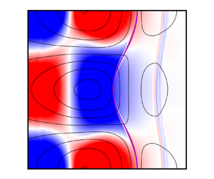
The evolution of the electron fluid largely decides the severity of the RMI in finite skin depth plasmas. It has been shown previously (Bond et al. Reference Bond, Wheatley, Samtaney and Pullin2017b; Tapinou et al. Reference Tapinou, Wheatley, Bond and Jahn2022) that (i) the absence of an electron density interface or (ii) the suppression of relative motion between the electron and ion fluids greatly reduces the severity of the RMI due to suppression of secondary instabilities. In the current work, point (ii) still occurs due to the presence of the interspecies collisions. However, both ions and electrons experience Lorentz force accelerations (of opposite sign to one another) from the applied magnetic field. The electrons experience a greater acceleration owing to their lesser mass and consequently the relative velocities, shown in figure 6, are more strongly influenced by Lorentz accelerations of the electron fluid rather than ion fluid. The increase in relative motion can generate stronger electromagnetic fields and drive secondary instabilities. In the cases studied here, any destabilising effect these increased relative velocities may have is dominated by the stabilising vorticity deposited on the interface by magnetic field torque.

Figure 6. Contour plots of relative velocity components in the (a,d,g to c,f,i)  $x$,
$x$,  $y$ and $z$ directions at 0.25 non-dimensional time. Applied magnetic field beta value of $\beta = \infty, 0.01\ \textrm{and}\ 0.001$ shown (a–c) to (g–i) for anisotropic cases. The ion–fluid density interface is shown overlayed in green.
3.4. Comparison to previous collisional plasma RMI results
The dual layer instability, previously observed for simulations at smaller length scales (Tapinou et al. Reference Tapinou, Wheatley, Bond and Jahn2023), is not excited in the current simulations. In the previous study (Tapinou et al. Reference Tapinou, Wheatley, Bond and Jahn2023) the dual-layer instability was initiated after a negative–positive dual layer in charge distribution was formed on the density interface. After shock traversal of the density interface, significant current densities preceded the formation of filaments of high-density fluid penetrating the interface, attempting to neutralise the dual layer. The instability only occurred in the anisotropic simulations, where inhomogeneous transport coefficients along the extent of the interface allowed variable resistance to the filamentation thereby allowing the instability to grow from the spike and along the extent of the interface. In the current simulations, the dual-layer instability is not observed, possibly due to the same reason the isotropic and anisotropic simulations produce little difference in the current work. Further work is required to characterise the dual-layer instability and will be a subject of future work.
4. Driving mechanisms
This section explores the driving mechanisms for stabilisation of the plasma RMI by the applied magnetic field. Conclusions from previous work on the ideal MFP RMI with applied magnetic field (Bond et al. Reference Bond, Wheatley, Li, Samtaney and Pullin2020) and collisional MFP RMI without magnetic field (Tapinou et al. Reference Tapinou, Wheatley, Bond and Jahn2023) are used to elucidate the effect of the magnetic field on the collisional case. The objective is to determine whether there are fundamental differences in the stabilising action of the magnetic field in the collisional case. Some small differences in the macroscopic effect were discussed in the previous section, here they are discussed in detail.
4.1. Contributions to interface circulation
The contributions to the density interface circulation are a combination of the sources characterised in previous work (Bond et al. Reference Bond, Wheatley, Li, Samtaney and Pullin2020; Tapinou et al. Reference Tapinou, Wheatley, Bond and Jahn2023) and there is no new emergent phenomena from the combination of magnetic field and the collisional terms. Figure 7 shows, for the anisotropic  $\beta =0.001$ case, the RMI perturbation width and growth rate, total circulation and effects contributing to the circulation time rate of change for the region constituting the interface. Due to the symmetry in density interface circulation about the $x$-axis, the summation over a half-period of the interface is taken, in our case we analyse the lower half of the interface below the $x$-axis. The interface is defined as the region utilising the tracer variable (mixture fraction) as described below. The vorticity equation is
 \begin{align} \frac{{\rm D}
\boldsymbol{\omega}}{{\rm D} t} &= \underbrace{
(\boldsymbol{\omega}\boldsymbol{\cdot}\boldsymbol{\nabla})\boldsymbol{u}
}_{\dot{\varGamma}_{str}}
-\underbrace{\boldsymbol{\omega}\left( \boldsymbol{\nabla}
\boldsymbol{\cdot} \boldsymbol{u} \right)
}_{\dot{\varGamma}_{comp}} +
\underbrace{\frac{1}{\rho_\alpha^2}\left(\boldsymbol{\nabla}{\rho_\alpha}\times
\boldsymbol{\nabla}{p_\alpha}\right)
}_{\dot{\varGamma}_{baro}}\nonumber\\
&\quad+\underbrace{\boldsymbol{\nabla}\times{\left(\sqrt{\frac{2}{\beta}}\frac{q_\alpha}{d_S
m_\alpha} \left(c\boldsymbol{E}+\boldsymbol{u}_\alpha
\times \boldsymbol{B}\right)\right)}
}_{\dot{\varGamma}_{L,E} + \dot{\varGamma}_{L,B}}
+\underbrace{\boldsymbol{\nabla}\times \left(\vphantom{\sqrt{\frac{2}{\beta}}}
\frac{1}{\rho_\alpha} \left(\vphantom{\sqrt{\frac{2}{\beta}}}\begin{matrix}\displaystyle\boldsymbol{\nabla}\boldsymbol{\cdot}{\overleftrightarrow{\varPi}_\alpha}
+\sum_{\zeta\!\!\neq\alpha}\boldsymbol{R}_{\alpha\zeta}\end{matrix}\right)\right)}_{\dot{\varGamma}_{visc} +
\dot{\varGamma}_{drag}}, \end{align}
\begin{align} \frac{{\rm D}
\boldsymbol{\omega}}{{\rm D} t} &= \underbrace{
(\boldsymbol{\omega}\boldsymbol{\cdot}\boldsymbol{\nabla})\boldsymbol{u}
}_{\dot{\varGamma}_{str}}
-\underbrace{\boldsymbol{\omega}\left( \boldsymbol{\nabla}
\boldsymbol{\cdot} \boldsymbol{u} \right)
}_{\dot{\varGamma}_{comp}} +
\underbrace{\frac{1}{\rho_\alpha^2}\left(\boldsymbol{\nabla}{\rho_\alpha}\times
\boldsymbol{\nabla}{p_\alpha}\right)
}_{\dot{\varGamma}_{baro}}\nonumber\\
&\quad+\underbrace{\boldsymbol{\nabla}\times{\left(\sqrt{\frac{2}{\beta}}\frac{q_\alpha}{d_S
m_\alpha} \left(c\boldsymbol{E}+\boldsymbol{u}_\alpha
\times \boldsymbol{B}\right)\right)}
}_{\dot{\varGamma}_{L,E} + \dot{\varGamma}_{L,B}}
+\underbrace{\boldsymbol{\nabla}\times \left(\vphantom{\sqrt{\frac{2}{\beta}}}
\frac{1}{\rho_\alpha} \left(\vphantom{\sqrt{\frac{2}{\beta}}}\begin{matrix}\displaystyle\boldsymbol{\nabla}\boldsymbol{\cdot}{\overleftrightarrow{\varPi}_\alpha}
+\sum_{\zeta\!\!\neq\alpha}\boldsymbol{R}_{\alpha\zeta}\end{matrix}\right)\right)}_{\dot{\varGamma}_{visc} +
\dot{\varGamma}_{drag}}, \end{align}
where the evolution terms from left to right are the effect of stretching/tilting due to velocity gradients ( $\dot {\varGamma }_{str}$, zero in $z$-dimensions for two dimensions), stretching due to flow compressibility ( $\dot {\varGamma }_{comp}$), baroclinic generation ( $\dot {\varGamma }_{baro}$) that is the primary driver of RMI growth, the electric ( $\dot {\varGamma }_{L,E}$) and magnetic field ( $\dot {\varGamma }_{L,B}$) torques, and viscous dissipation ( $\dot {\varGamma }_{visc}$), and interspecies drag terms ( $\dot {\varGamma }_{drag}$). These terms are calculated in a postprocessing step using a heuristic to estimate the density interface region. The heuristic uses the volume of fluid tracer, $\varrho$, value that is convected with the flow and fluid properties related to the circulation source terms. The threshold of tracer value in the $x$-direction, $(0.05, 0.95)$, is used to establish a preliminary search area, after which the magnitude of mass-density gradient, $|\textrm {d}\rho /{\textrm {d}\kern0.06em x}|$, and charge density, $q$, are used to establish the final interface region, accounting for hydrodynamic and electromagnetic sources of circulation, respectively. The location of peak of mass-density gradient magnitude and charge density within the preliminary search area is used to expand the preliminary region. The maximum spatial extents corresponding to threshold values of 5 % of peak values are used to establish a final density interface region, for a discrete $y$-dimension point. This procedure is followed for each discrete point in the $y$-dimension until the entire interface region is identified. We note that while this heuristic is useful in finding contributions of terms affecting the rate of change of circulation, it is imperfect. It is used as an indicator of behaviour, not an accurate quantitative metric. An example of the interface heuristic is shown in figure 8. The value of circulation and the evolution terms within each cell are summed, individually, and the resulting time series shows the influence on the interface evolution. These metrics, though useful for investigating the interface behaviour, do not exactly correspond to growth rate and perturbation width values on their own since the interface evolution is also affected by vorticity beyond what are considered the extents of the interface.

Figure 7. Interface analysis for the  $\beta =0.001$ case with anisotropic modelling. Here, $\dot {\varGamma }$ and $\varGamma$ are the time rate of change and instantaneous circulation, respectively, of a half-period of the density interface below the $x$-axis, and $\eta$ and $\dot {\eta }$ are the instantaneous and time rate of change of the density interface perturbation width (not amplitude).

Figure 8. An example of the interface heuristic, where the region coloured grey is characterised by the volume of fluid tracer, and the region in red is characterised by the thresholds of density gradient and charge density.
Returning to figure 7, each of the circulation evolution terms in (4.1) vary in strength, activity and effect during the simulation. We distinguish here between a single term's contribution at a point and the accumulative contribution of a term across all points comprising the interface, our analysis refers to the latter. There is non-zero activity from  $\dot {\varGamma }_{visc}$ and $\dot {\varGamma }_{drag}$ at simulation initialisation due to the discontinuity in temperature on the interface that drives motion and heat exchange. The collisional circulation terms are related to the strain rate within each (intraspecies) and the relative velocity between fluids (interspecies). After the simulation begins the collisional terms spike due to the dissipative waves emitted from the interface and the large area the heuristic includes in the interface summation. Following this spike, $\dot {\varGamma }_{visc}$ is strongest during the shock passage, resisting the intense strain rates the fluid experiences. $\dot {\varGamma }_{drag}$ oscillates in sign depending on the relative velocities of the ion and electron fluids, and is much larger for the electrons due to their smaller mass. The $\dot {\varGamma }_{baro}$ term is the most dominant non-collisional term and is initially generated during shock traversal of the density interface that initiates the RMI. After shock traversal, $\dot {\varGamma }_{baro}$ results from the secondary electromagnetically driven Rayleigh–Taylor instability (ERTI).
The magnetic field torque generates circulation on the interface, and the accumulation of circulation from this source over half the interface is represented by  $\dot {\varGamma }_{L,B}$. Here $\dot {\varGamma }_{L,B}$ increases across scenarios with applied magnetic field, since the self-generated magnetic field produces negligible contributions. Here $\dot {\varGamma }_{L,B}$ directly opposes $\dot {\varGamma }_{baro}$, most intensely during shock traversal but also continuously thereafter, supporting the trend from the ideal MFP MRI with applied magnetic field (Bond et al. Reference Bond, Wheatley, Li, Samtaney and Pullin2020). Here $\dot {\varGamma }_{L,E}$ is small in comparison, during the entire simulation despite the dual layer in charge density (Tapinou et al. Reference Tapinou, Wheatley, Bond and Jahn2023) that is present on the interface, likely due to the symmetry of the resulting electric field about the density interface. All these terms combine to influence the evolution of the RMI perturbation growth. Further development of the interface heuristic is required as we do not consider it accurate at this time. However, it does provide some insight into the interface dynamics and has potential for improvement.
The magnetic field also affects the plasma RMI evolution through influencing the relative motion between the fluids. In previous work (Bond et al. Reference Bond, Wheatley, Samtaney and Pullin2017b, Reference Bond, Wheatley, Li, Samtaney and Pullin2020; Tapinou et al. Reference Tapinou, Wheatley, Bond and Jahn2022, Reference Tapinou, Wheatley, Bond and Jahn2023) the electron fluid behaviour was found to be crucial in self-generating electromagnetic fields and exciting the ion fluid density interface. In the current work we find that increasing the applied  $x$-magnetic field leads to a modest increase in magnitude of the relative motion, mostly through the Lorentz accelerations of the electron fluid. The combination of the resulting current densities and the spatial variations in the magnetic fields, i.e. equation (2.6b) alters the electric field that influence secondary instabilities. The interface analysis shows that the applied magnetic field directly opposes the baroclinic vorticity deposition on the interface in both the electron and ion fluids, figure 7. The exact effect on ERTI from the change in electric fields, resulting from the increased relative motion, is not known and is left to future investigation. However, it is clear the magnetic torque $\tau _B$ dominates the suppression of the RMI relative to the unmagnetised case.
4.2. Anisotropy in transport coefficients
The interface statistics, figure 9, show that modelling transport coefficient anisotropy increases the instability growth relative to the isotropic cases for all values of  $\beta$. In the $\beta =\infty, 0.01,\textrm { and }0.001$ case the relative increase in interface perturbation width is $7.7\,\%$, $3.8\,\%$ and $4.4\,\%$, respectively. This trend was observed in previous work (Tapinou et al. Reference Tapinou, Wheatley, Bond and Jahn2023) and is reproduced for applied magnetic fields. Consider for example (A9) which show the relations defining the parallel, perpendicular and diamagnetic transports coefficients for the inter species drag. Note the perpendicular and diamagnetic terms are nonlinear in Hall parameter. The transverse (relative to the magnetic field) transport coefficients are generally smaller than the parallel ones, and so depending on the directions of the magnetic field and relevant fluid property, the collisional effects are reduced (in magnitude) for some directions, thus making possible increased growth. The increase in growth with anisotropy, i.e. the difference between anisotropic and isotropic RMI perturbation width, is reduced when a $x$-magnetic field is applied (as does the overall growth). The decrease in growth enhancement due to anisotropy, as discussed in the preceding section, is due to the magnetic field parallel direction (combination of applied and self-generated fields) becoming increasingly $x$-aligned thereby affecting the transport phenomena less as they themselves are most aligned in the $x$-direction due to the directional flow field and temperature gradients.

Figure 9. Summary interface vorticity statistics for the scenarios simulated (isotropic and anisotropic cases represented with ‘I’ and ‘A’, respectively). Here  $\dot {\varGamma }$ instantaneous circulation of a half-period of the density interface below the $x$-axis, and $\eta$ and $\dot {\eta }$ are the instantaneous and time rate of change of the density interface perturbation width (not amplitude).
4.3. Ion and electron circulation behaviour at threshold magnetic field strength
In figure 7 we see a significant difference between the electron and ion circulation for the anisotropic  $\beta =0.001$ scenario at simulation end. This difference in final time circulation is greater relative to the preceding anisotropic cases ( $\beta =\infty \textrm { and }0.01$), figure 10. The difference between the ion and electron fluid density interface circulation, relative to the electron fluid density interface circulation is 77.0 %, 19.2 % and 11.3 % in the strong, moderate and zero magnetic field case. This disparity between the electron and ion circulation is not as significant in the isotropic $\beta = 0.001$ simulation. The Hall parameter is a comparative measure of gyroscopic and collisional effects. This parameter in the low-density ion fluid, for the $\beta =0.001$ and $\beta =0.01$ cases, are $\omega _{c,i}\tau _i\approx 0.403\textrm { and }0.128$ and for the electrons $\omega _{c,e}\tau _e\approx 2.852\textrm { and }0.901$. On the high-density side they are $\omega _{c,i}\tau _i\approx 0.009\textrm { and }0.003$, and for the electrons $\omega _{c,e}\tau _e\approx 0.951\textrm { and }0.300$. The plasma surrounding the density interface experiences several different regimes, according to the Hall parameters. In the two magnetised cases we may expect the electrons to always be either moderately or strongly affected by gyroscopic motion. The ions, however, experience weakly to moderate gyroscopic effects on the high and low density regions that comprise the interface. It may be that, for the strongest magnetic field case, the change in relative ion and electron circulation profiles observed represents a threshold magnetic field value as indicated by Hall parameter values. This threshold may be where ion gyroscopic effects begin to introduce additional differences between the ion and electron fluids, whereas in the lesser magnetic field values the ion gyroscopic effects are negligible in this regard. It will be interesting to investigate further the magnetic field parameter space with intermediate and stronger $\beta$ values, to clarify further the influence of gyroscopic effects on RMI evolution.

Figure 10. Density interface circulation time series for the ion and electron (ele) fluids with anisotropic transport coefficients.
4.4. Secondary vorticity suppression mechanisms
The interface vorticity suppression mechanism in the magnetised collisional MFP RMI studied here is significantly different from the ideal case. Here, the collisional effects are highly dissipative and consequently reduce vorticity in the flow field and along the density interface. In the ideal magnetised MFP RMI by Bond et al. (Reference Bond, Wheatley, Li, Samtaney and Pullin2020), the vorticity vector exhibits highly periodic behaviour (rotating spatially) and the density interface sheds vorticity waves in the small Debye length case. In the present work, some small periodicity is observed within the interface circulation components but this is negligible in comparison with the periodicity in the ideal magnetised MFP RMI. Figures 11 and 12 show the accumulated vorticity on the density interface for the  $\beta =0.01$ and $\beta =0.001$ anisotropic cases. The $\beta =0.001$ case may be showing the first period of a similar oscillatory behaviour but the simulation ends before this is confirmed. Figure 13 shows the $z$-component of ion vorticity at the midpoint on the density interface halfway between the spike and bubble. Compared with the results of Bond et al. (Reference Bond, Wheatley, Li, Samtaney and Pullin2020), which are presented in Appendix A (see figure 14), we see the vorticity vector rotation phenomena are not reproduced in the present collisional results.

Figure 11. The total interface circulation components (over the lower half-period of the interface) in all three spatial dimensions for the anisotropic  $\beta =0.01$ case.

Figure 12. The total interface circulation components (over the lower half-period of the interface) in all three spatial dimensions for the anisotropic  $\beta =0.001$ case.

Figure 13. Evolution of ion vorticity for the  $d_D=2.08\times 10^{-3}$ and $\beta =0.001$ anisotropic case sampled at a point fixed to the interface approximately midway between the bubble and the spike.

Figure 14. Evolution of ion vorticity and torque due to the magnetic field for  $d_D=2\times 10^{-3}$ and $\beta =0.1$ sampled at a point fixed to the interface approximately midway between the bubble and the spike. Surface plot shows the vector of interest with displacement along the $x$-axis by the sample time $t$. (a) Vorticity vector and (b) magnetic field.
The vorticity waves observed in the ideal MFP case (Bond et al. Reference Bond, Wheatley, Li, Samtaney and Pullin2020) (after shock traversal of the interface) alternated in the sign of vorticity that was swept away from the interface. For the large Debye length cases ( $\lambda _D=2\times 10^{-1}\textrm { and }2\times 10^{-1}$), the waves were diffuse, whereas for smaller Debye length ( $\lambda _D=2\times 10^{-1}$) the wave packets became concentrated (Bond et al. Reference Bond, Wheatley, Li, Samtaney and Pullin2020). Significant vorticity carrying waves are not observed in the present simulations. There are regions of low magnitude diffuse vorticity in the flow field trailing the transmitted and reflected shocks but this is likely due to the non-planar shock front that propagates away from the interface, rather than transported vorticity from the interface. The absence of this mechanism is consistent with the inclusion of elastic collisions in the MFP equations since these terms dominate the vorticity evolution after the incident shock traverses the interface. The dissipation of vorticity by the collisional terms and direct deposition of stabilising vorticity by the magnetic field torque supersedes the transport of vorticity by waves.
The collisional effects prevent the plasma from manifesting the vorticity rotation and transport of vorticity by waves but the physical mechanisms that drive these manifestations is still present. The rotation of the vorticity vector is caused by the magnetic component of the Lorentz force  $\mathcal {L} = n_\alpha \, q_\alpha \, \boldsymbol {u_\alpha }\times \boldsymbol {B}$ giving an out of plane velocity component to the fluids. The acceleration within the ion and electrons fluids is opposite due to the sign of charge. This results in a vorticity rotation in opposite directions, but more significantly for the collisional case is that there is relative motion between the ion and electrons fluids. This relative motion is strongly opposed by the interspecies drag term that kills off the out of plane velocity and consequently the vorticity rotation. The vorticity waves observed in the ideal cases for varying Debye lengths appear to experience nonlinear wave steepening, trending towards discontinuous waves in the limit of vanishing Debye length. The viscous dissipation of vorticity by the elastic collisions in the present case obstructs the propagation of vorticity waves and any wave steepening that would produce the concentrated wave packets of vorticity observed in the ideal case. Therefore, the collisional MFP RMI studied in the present work does not manifest the vorticity suppression mechanisms observed in the ideal case (Bond et al. Reference Bond, Wheatley, Li, Samtaney and Pullin2020). The driving mechanism for the vorticity vector rotation and vorticity transport by waves is still permitted but the dissipation by collisional effects dominates.
4.5. Comparison with MHD relations for RMI growth
Predictions for the primary perturbation amplitude according to ideal MHD theory were found to be inaccurate for the present work. Wheatley et al. (Reference Wheatley, Samtaney and Pullin2009) derived expressions for the amplitude by linearising the equations of ideal MHD, assuming incompressible fluid, and modelling the shock acceleration of the interface as a velocity impulse. The resulting expressions give the perturbation amplitude as a function of time and the late time asymptotic amplitude, they have the form
 \begin{equation} \eta_\infty =
\eta_0\Big(1 + \frac{V}{B}\Big(\rho_2^{0.5} -
\rho_1^{0.5}\Big)\Big) \end{equation}
\begin{equation} \eta_\infty =
\eta_0\Big(1 + \frac{V}{B}\Big(\rho_2^{0.5} -
\rho_1^{0.5}\Big)\Big) \end{equation}and
 \begin{equation} \eta(t) = \eta_\infty - \left(\eta_\infty - \eta_0\right) \exp\left(\sigma\,t\right)\cos\left(\tau t\right), \end{equation}
where  $\eta$ here is the perturbation amplitude. The theory predicts, for the $\beta =0.001$ and $\beta =0.01$ cases, perturbation amplitudes that are almost completely suppressed, where $\eta _\infty =0.1021\ \textrm {and}\ 0.1066$. At the simulation's end, the $\beta =0.001$ and $\beta =0.01$ cases have a perturbation amplitude of $0.1167$ and $0.1547$, respectively. Note that figure 9 shows the perturbation width, twice the amplitude. In deriving the incompressible linearised model Wheatley et al. (Reference Wheatley, Samtaney and Pullin2009) the perturbed streamwise velocity and magnetic field components are constrained to be continuous across the contact discontinuity. This condition permits Alfvén waves in the solution that transport significant vorticity from the density interface. The model assumes that the Alfvén waves propagate slower than the sound's speed which is not the case in the present simulations either. In MFP simulations the transport of vorticity by waves is not observed, accounting for the increased interface amplitude growth when comparing with the model prediction.
5. Conclusion
An applied magnetic field, aligned with the shock wave direction, significantly alters the evolution of the RMI of a collisional MFP. Three scenarios were considered, the case of no applied magnetic field and a moderate and strong magnetic field strength. The magnetic-field-induced anisotropy was studied by comparing the cases with and without anisotropic modelling. The simulation results show that modelling magnetic field anisotropy produces increased RMI growth rates, supporting previous results by Tapinou et al. (Reference Tapinou, Wheatley, Bond and Jahn2023) which are due to a reduction in transport coefficients in the magnetic field perpendicular directions. The influence of magnetic-field-induced anisotropy is reduced as the  $x$-magnetic field strength increases because of the size and direction of self-generated magnetic fields relative to the applied field. Generally, applying a significant magnetic field ( $\beta \leq 0.01$) suppresses the RMI. The dual layer instability, previously observed at smaller length scales (Tapinou et al. Reference Tapinou, Wheatley, Bond and Jahn2022), does not occur in the present scenario. In the strong field case, $\beta =0.001$, the ion circulation on the density interface may be experiencing more significant gyroscopic effects (small Larmor radius effects) in comparison with the preceding case but further investigation is required. The vorticity suppression mechanisms observed in the ideal case (Bond et al. Reference Bond, Wheatley, Li, Samtaney and Pullin2020), i.e. the rotation of the vorticity vector and transport of vorticity via waves, do not manifest in the present collisional cases as the dissipation of vorticity by the collisional terms is the dominant mechanism. The applied magnetic field increases relative motion between the fluids but not sufficiently to destabilise the primary perturbation through secondary ERTI or EM field torques. The suppression of the primary RMI in the ion fluid is due to the direct contribution of $\tau _B$ on the density interface and the collisional terms. Our results indicate that modelling the magnetic-field-induced anisotropy may only be important when the flow properties influencing the transport coefficients have significant component in the field perpendicular direction, a possible modelling simplification for future applications. The simulation results presented here are for collisional plasmas with low Reynolds numbers. It is expected that higher Reynolds number flows, given finite Debye length present, would permit secondary KHI and allow MFP effects (secondary ERTI, excitation of ion fluid by electrons, and other effects (Tapinou et al. Reference Tapinou, Wheatley, Bond and Jahn2022)) to manifest more significantly. However, we expect the magnetic field stabilisation of the instability to remain effective since the primary mechanism is independent of the collisional terms modelled here. The works completed show that the MFP RMI in a collisional plasma can be suppressed effectively by an applied magnetic field, in the shock direction.
Declaration of interests
The authors report no conflict of interest.
Data availability statement
The data that support the findings of this study are available from the corresponding author upon reasonable request. The numerical tool, Ceberus, that was used to run the simulations investigated in this work are available at the Github repository: https://github.com/PlasmaSimUQ/cerberus.
Appendix A
A.1. Braginskii transport model
The equations of the Braginksii's transport model (Braginskii Reference Braginskii1965) approximate the local solution of the kinetic equation for each species. A two term Sonine (or Laguerre) polynomial is used to approximate the distribution functions. Numerical inaccuracies arise from the truncation of the polynomial terms and the polynomial fit. The fundamental approach is to obtain separate transport coefficients for the electrons and ions with different temperatures and velocities that are decoupled. The resulting equations have (i) ion distribution with dependence on self-interactions, and (ii) electron distribution with a dependence on the self- and cross-interactions. The numerical coefficients that make up the Braginskii transport coefficients are calculated exactly (after the Sonine polynomials are taken to the second term) and reported with rational numbers.
The key assumptions used in the derivation are as follows. General conservation of the collision integral across the moments taken such that the number of particles, momentum-density and energy-density is conserved in like species collisions and dissimilar species collisions. The distribution functions of the species take the form of a Maxwellian distribution. All quantities vary slowly in space and in time, i.e. change must be on a length scale larger/longer than the mean free path between collisions and slower than the collision time scale. The dominant term in the kinetic equations are the collision operators and the magnetic field term. It is assumed the magnetic field does not affect the collision integral, i.e. the radius of curvature, the Larmor radius, is large compared with the Debye length. The mass ratio of the ions and electrons is small. The difference in the mean velocities of ions and electrons is small compared with the characteristic electron velocity. The derivation neglects the effects of inelastic collisions such as those resulting in ionisation, fusion, recombination, excitation/de-excitation of internal degrees of freedom, and the Landau collision operator does not consider the effect of magnetic fields on itself.
The largest error in the approximation of the transport coefficient is in the regime where the product of the cyclotron frequency and the collision time scale is of order one. These errors can be as great as 10 to 20 per cent (Braginskii Reference Braginskii1965). Since Braginskii's seminal work, several authors have revised the calculation of some of the transport coefficients (typically with respect to accuracy or functional form/physical behaviour in limits of strong magnetic fields  $\omega \tau \rightarrow \infty$) (Epperlein & Haines Reference Epperlein and Haines1986; Davies et al. Reference Davies, Wen, Ji and Held2021). Some specific constructive criticisms are the (i) over-estimation of advection due to perpendicular resistivity, $\eta _{\perp }$ in Braginskii's data fits (Davies et al. Reference Davies, Wen, Ji and Held2021), (ii) inaccuracy of $\beta _{}$, $\kappa _{\perp }$ and $\kappa _{}$ in the range of $0.3 \geq \omega \tau \geq 30$ (Epperlein & Haines Reference Epperlein and Haines1986), among others. We continue with the Braginskii result for simplicity and the ubiquitous comparisons available in the literature while acknowledging their accuracy is limited for some parameter regimes though certainly instructive for the fundamental plasma behaviours.
In the following non-dimensionalised equations, note that  $d_{d,0}$ and $d_{L,0}$ are the non-dimensional reference Debye length and Larmor radius, respectively, and $\hat {n}_0$ is the product of reference number density and reference length cubed ( $\hat {n}_0 = n_0x_0^3$). The characteristic collision time scales are the ion and electron collision times $\tau _e$ and $\tau _i$, given by
 $$\begin{gather} \tau_e = d^4_{d,0}\hat{n}_0\frac{6\sqrt{2}m^{1/2}_e({\rm \pi} T_e)^{3/2}}{\ln(\varLambda)n_iZ^2q_e^4}, \end{gather}$$
 $$\begin{gather}\tau_i = d^4_{d,0}\hat{n}_0\frac{12m^{1/2}_i({\rm \pi} T_i)^{3/2}}{n_iZ^4q_e^4\ln(\varLambda)}. \end{gather}$$
The cyclotron frequencies in the ion and electron fluids govern the magnetic influence on collisions and are given by
 $$\begin{gather} \omega_{c,e} = \frac{q_eB}{m_e}\frac{1}{d_{L,0}}, \end{gather}$$
 $$\begin{gather}\omega_{c,i} = \frac{q_eZB}{m_i}\frac{1}{d_{L,0}}. \end{gather}$$
 In the following transport coefficients we will refer to the components parallel and perpendicular to the local magnetic field, and to the diamagnetic terms. The diamagnetic terms generally refer to transport properties that arise due to imbalances in momentum or energy when counter-propagating fluids interact at a common point within their gyro-orbits. The direction of the resulting net momentum or energy change is perpendicular to both the magnetic field and the instigating property, i.e. relative velocity or temperature gradient. The parallel, perpendicular and diamagnetic terms are denoted by a subscript  $\parallel$, $\perp$ and $\bigwedge$, respectively. It is important to note the following equations are all non-dimensional according to the previous non-dimensionalisation:
 \begin{equation} \left. \begin{aligned}
\varPi_0 & = \rho_0 u_0^2, \quad \hskip9pt q_0 = \rho_0
u_0^3, \hskip8.5pt\quad Q_0 = \frac{\rho_0
u_0^3}{x_0}, \quad \hskip4pt R_0 = \frac{\rho_0
u_0^2}{x_0}, \\ \eta_0 & = \rho_0 x_0
u_0, \quad \kappa_0 = \frac{u_0
k_B}{x_0^2}, \quad \beta_0^{TU} = \rho_0
u_0^3, \quad \beta^{UT}_0 = n_0, \\
\alpha_0 & = \frac{\rho_0 u_0}{x_0}.
\end{aligned} \right\}
\end{equation}
\begin{equation} \left. \begin{aligned}
\varPi_0 & = \rho_0 u_0^2, \quad \hskip9pt q_0 = \rho_0
u_0^3, \hskip8.5pt\quad Q_0 = \frac{\rho_0
u_0^3}{x_0}, \quad \hskip4pt R_0 = \frac{\rho_0
u_0^2}{x_0}, \\ \eta_0 & = \rho_0 x_0
u_0, \quad \kappa_0 = \frac{u_0
k_B}{x_0^2}, \quad \beta_0^{TU} = \rho_0
u_0^3, \quad \beta^{UT}_0 = n_0, \\
\alpha_0 & = \frac{\rho_0 u_0}{x_0}.
\end{aligned} \right\}
\end{equation}A.1.1. Interspecies drag forces
The interspecies forces due to friction and temperature gradients – temperature gradients introduce a diamagnetic effect due to the difference in energies of fluid interacting in opposing gyro-orbits – are denoted by subscript ‘U’ and ‘T’, respectively, and are given by
 $$\begin{gather} \boldsymbol{R}_{U} =-\alpha_{{\parallel}}\boldsymbol{u}_{{\parallel}} - \alpha_{{\perp}}\boldsymbol{u}_{{\perp}} -\alpha_{\bigwedge}\boldsymbol{u}_{\bigwedge}, \end{gather}$$
 $$\begin{gather}\boldsymbol{R}_T =-\beta^{UT}_{{\parallel}}\boldsymbol{\nabla}_{{\parallel}}T_e -\beta^{UT}_{{\perp}}\boldsymbol{\nabla}_{{\perp}}T_e - \beta^{UT}_{\bigwedge}\boldsymbol{\nabla}_{\bigwedge}T_e, \end{gather}$$
here  $\boldsymbol {u}$ the relative velocity between the electron and ion fluids, $\boldsymbol {u}=\boldsymbol {u}_e-\boldsymbol {u}_i$. The thermal force is only dependent on the electron temperature gradient because the relative velocity which sets the rate of collisions between electrons and ions is dominated by the more mobile electrons. The constants and vector definitions of each direction are as follows:
 \begin{gather} \left.
\begin{array}{ll@{}} \hskip3pt\boldsymbol{u}_{{\parallel}} =
\dfrac{\boldsymbol{B}}{{\left|B\right|}} \left(
\boldsymbol{u}\boldsymbol{\cdot}\dfrac{\boldsymbol{B}}{{\left|B\right|}}
\right), & \hskip2pt\boldsymbol{\nabla}_{{\parallel}}T_e =
\dfrac{\boldsymbol{B}}{{\left|B\right|}} \left(
\boldsymbol{\nabla}
T_e\boldsymbol{\cdot}\dfrac{\boldsymbol{B}}{{\left|B\right|}}\right),
\\ \hskip1pt\boldsymbol{u}_{{\perp}} =
\boldsymbol{u} - \boldsymbol{u}_{{\parallel}}, &
\boldsymbol{\nabla}_{{\perp}} T_e = \boldsymbol{\nabla} T_e
- \boldsymbol{\nabla}_{{\parallel}} T_e,
\\ \boldsymbol{u}_{\bigwedge} =
\dfrac{\boldsymbol{B}}{{\left|B\right|}} \times
\boldsymbol{u}, & \hskip-1pt\boldsymbol{\nabla}_{\bigwedge}
T_e = \dfrac{\boldsymbol{B}}{{\left|B\right|}} \times
\boldsymbol{\nabla} T_e; \end{array} \right\}
\end{gather}
\begin{gather} \left.
\begin{array}{ll@{}} \hskip3pt\boldsymbol{u}_{{\parallel}} =
\dfrac{\boldsymbol{B}}{{\left|B\right|}} \left(
\boldsymbol{u}\boldsymbol{\cdot}\dfrac{\boldsymbol{B}}{{\left|B\right|}}
\right), & \hskip2pt\boldsymbol{\nabla}_{{\parallel}}T_e =
\dfrac{\boldsymbol{B}}{{\left|B\right|}} \left(
\boldsymbol{\nabla}
T_e\boldsymbol{\cdot}\dfrac{\boldsymbol{B}}{{\left|B\right|}}\right),
\\ \hskip1pt\boldsymbol{u}_{{\perp}} =
\boldsymbol{u} - \boldsymbol{u}_{{\parallel}}, &
\boldsymbol{\nabla}_{{\perp}} T_e = \boldsymbol{\nabla} T_e
- \boldsymbol{\nabla}_{{\parallel}} T_e,
\\ \boldsymbol{u}_{\bigwedge} =
\dfrac{\boldsymbol{B}}{{\left|B\right|}} \times
\boldsymbol{u}, & \hskip-1pt\boldsymbol{\nabla}_{\bigwedge}
T_e = \dfrac{\boldsymbol{B}}{{\left|B\right|}} \times
\boldsymbol{\nabla} T_e; \end{array} \right\}
\end{gather} \begin{gather} \left.
\begin{array}{ll@{}} \hskip3pt\alpha_{{\parallel}} =
\rho_e\nu_e{\alpha}_0, & \beta^{UT}_{{\parallel}}
= n_e\beta_0, \\
\alpha_{{\perp}} =
\rho_e\nu_e\dfrac{1-\alpha'_1x_e^2+\alpha_0}{\Delta_e},
& \beta^{UT}_{{\perp}} = n_e\dfrac{1-\beta'_1
x_e^2+\beta'_0}{\Delta_e}, \\
\hskip-1pt\alpha_{\bigwedge} = \rho_e\nu_e
x_e\dfrac{\alpha''_2x_e^2+\alpha''_0}{\Delta_e},
& \beta^{UT}_{\bigwedge}= n_e x_e\dfrac{\beta''_1 x_e^2 +
\beta''_0}{\Delta_e}. \end{array} \right\}
\end{gather}
\begin{gather} \left.
\begin{array}{ll@{}} \hskip3pt\alpha_{{\parallel}} =
\rho_e\nu_e{\alpha}_0, & \beta^{UT}_{{\parallel}}
= n_e\beta_0, \\
\alpha_{{\perp}} =
\rho_e\nu_e\dfrac{1-\alpha'_1x_e^2+\alpha_0}{\Delta_e},
& \beta^{UT}_{{\perp}} = n_e\dfrac{1-\beta'_1
x_e^2+\beta'_0}{\Delta_e}, \\
\hskip-1pt\alpha_{\bigwedge} = \rho_e\nu_e
x_e\dfrac{\alpha''_2x_e^2+\alpha''_0}{\Delta_e},
& \beta^{UT}_{\bigwedge}= n_e x_e\dfrac{\beta''_1 x_e^2 +
\beta''_0}{\Delta_e}. \end{array} \right\}
\end{gather} Within (A9),  $x_e=\omega _{c,e}\tau _e$ and $\Delta _e = x_e^4 + \delta _1x_e^2+\delta _0$. The coefficients for a $Z=1$ plasma are $\alpha _0=0.5129$, $\alpha '_0=6.461$, $\alpha '_0=1.837$, $\alpha ''_0=0.7796$, $\delta _0=3.7703$ and $\delta _1=14.79$. Coefficients for greater atomic numbers are available in Braginskii (Reference Braginskii1965) (the values for $Z=1$ and $Z=3$ are utilised in this study). Note that $x_e$ and $\Delta _e$ are dimensionless numbers and the non-dimensionalisation of frequency and time are inverses and therefore there are no residual dimensional coefficients.
A.1.2. Viscous stress tensor
The viscous stress tensor is calculated following the approach of Li & Livescu (Reference Li and Livescu2019). The strain-rate tensor is calculated in the simulation reference frame and then transformed into the magnetic field aligned reference frame. The viscous stress tensor is then calculated as per Braginskii's derivation, which assumes the magnetic field aligned reference frame. Finally the stress tensor is then transformed back to the simulation reference frame. The strain-rate tensor is given by
 \begin{equation} \overleftrightarrow{\boldsymbol{W}}_\alpha = \boldsymbol{\nabla}\boldsymbol{u}_\alpha +\left(\boldsymbol{\nabla}\boldsymbol{u}_{\alpha}\right)^{\rm T} -\tfrac{2}{3}\left(\boldsymbol{\nabla}\boldsymbol{\cdot}\boldsymbol{u}_\alpha\right) \boldsymbol{I} \end{equation}
where  $\boldsymbol {I}$ is the identity matrix. The rotation matrix is given by $Q$, as follows:
 \begin{equation} Q = \hat{Q} = \begin{bmatrix} -b_y' & -b_x'b_z'' & b_x''\\ b_x' & -b_y'b_z'' & b_y''\\ 0 & b_x'b_x'' +b_y'b_y'' & b_z'' \end{bmatrix}. \end{equation}
Therefore, the strain-rate tensor in the magnetic field aligned reference frame is given by
 \begin{equation} \overleftrightarrow{W}_s'=Q^T\overleftrightarrow{W}_sQ. \end{equation}
Note the entries of the rotation matrix are unitless, formed by the ratio of magnetic field components and the magnetic field magnitude, given by
 \begin{equation} \left. \begin{array}{ll@{}} B'' = \dfrac{1}{|B|}, & B' = \dfrac{1}{\sqrt{B_x^2 + B_y^2}}, \\ b_x'' = B_xB'', & b_x' = B_xB',\\ b_y'' = B_yB'', & b_y' = B_yB',\\ b_z'' = B_zB''. & \end{array} \right\} \end{equation}
The viscous stress tensor in terms of the strain-rate tensor is given by
 \begin{equation} \left. \begin{aligned}
\overleftrightarrow{\varPi}_{0,0}' &=-\tfrac{1}{2}\eta_0
\left(\overleftrightarrow{\boldsymbol{W}}_{0,0}' +
\overleftrightarrow{\boldsymbol{W}}_{1,1}'\right)\\
&\quad -\tfrac{1}{2}\eta_1\left(\overleftrightarrow{\boldsymbol{W}}_{0,0}'
- \overleftrightarrow{\boldsymbol{W}}_{1,1}'\right)
-\eta_3\overleftrightarrow{\boldsymbol{W}}_{0,1}',\\
\overleftrightarrow{\varPi}_{0,1}'&=\overleftrightarrow{\varPi}_{1,0}'=-\eta_1\overleftrightarrow{\boldsymbol{W}}_{0,1}'
+\tfrac{1}{2}\eta_3\left(
\overleftrightarrow{\boldsymbol{W}}_{0,0}'-\overleftrightarrow{\boldsymbol{W}}_{1,1}'
\right),\\ \overleftrightarrow{\varPi}_{0,2}' &=
\overleftrightarrow{\varPi}_{2,0}'=-\eta_2\overleftrightarrow{\boldsymbol{W}}_{0,2}'
-
\eta_4\overleftrightarrow{\boldsymbol{W}}_{1,2}',\\
\overleftrightarrow{\varPi}_{1,1}' &=-\tfrac{1}{2}\eta_0\left(
\overleftrightarrow{\boldsymbol{W}}_{0,0}'
+\overleftrightarrow{\boldsymbol{W}}_{1,1}'\right)\\ &\quad -\tfrac{1}{2}\eta_1\left(
\overleftrightarrow{\boldsymbol{W}}_{1,1}'
-\overleftrightarrow{\boldsymbol{W}}_{0,0}'\right)
+\eta_3\overleftrightarrow{\boldsymbol{W}}_{0,1}',\\
\overleftrightarrow{\varPi}_{1,2}' &=\overleftrightarrow{\varPi}_{2,1}'=-\eta_2\overleftrightarrow{\boldsymbol{W}}_{1,2}'
+ \eta_4\overleftrightarrow{\boldsymbol{W}}_{0,2}',\\
\overleftrightarrow{\varPi}_{2,2}'&=-\eta_0\overleftrightarrow{\boldsymbol{W}}_{2,2}'.
\end{aligned} \right\}
\end{equation}
\begin{equation} \left. \begin{aligned}
\overleftrightarrow{\varPi}_{0,0}' &=-\tfrac{1}{2}\eta_0
\left(\overleftrightarrow{\boldsymbol{W}}_{0,0}' +
\overleftrightarrow{\boldsymbol{W}}_{1,1}'\right)\\
&\quad -\tfrac{1}{2}\eta_1\left(\overleftrightarrow{\boldsymbol{W}}_{0,0}'
- \overleftrightarrow{\boldsymbol{W}}_{1,1}'\right)
-\eta_3\overleftrightarrow{\boldsymbol{W}}_{0,1}',\\
\overleftrightarrow{\varPi}_{0,1}'&=\overleftrightarrow{\varPi}_{1,0}'=-\eta_1\overleftrightarrow{\boldsymbol{W}}_{0,1}'
+\tfrac{1}{2}\eta_3\left(
\overleftrightarrow{\boldsymbol{W}}_{0,0}'-\overleftrightarrow{\boldsymbol{W}}_{1,1}'
\right),\\ \overleftrightarrow{\varPi}_{0,2}' &=
\overleftrightarrow{\varPi}_{2,0}'=-\eta_2\overleftrightarrow{\boldsymbol{W}}_{0,2}'
-
\eta_4\overleftrightarrow{\boldsymbol{W}}_{1,2}',\\
\overleftrightarrow{\varPi}_{1,1}' &=-\tfrac{1}{2}\eta_0\left(
\overleftrightarrow{\boldsymbol{W}}_{0,0}'
+\overleftrightarrow{\boldsymbol{W}}_{1,1}'\right)\\ &\quad -\tfrac{1}{2}\eta_1\left(
\overleftrightarrow{\boldsymbol{W}}_{1,1}'
-\overleftrightarrow{\boldsymbol{W}}_{0,0}'\right)
+\eta_3\overleftrightarrow{\boldsymbol{W}}_{0,1}',\\
\overleftrightarrow{\varPi}_{1,2}' &=\overleftrightarrow{\varPi}_{2,1}'=-\eta_2\overleftrightarrow{\boldsymbol{W}}_{1,2}'
+ \eta_4\overleftrightarrow{\boldsymbol{W}}_{0,2}',\\
\overleftrightarrow{\varPi}_{2,2}'&=-\eta_0\overleftrightarrow{\boldsymbol{W}}_{2,2}'.
\end{aligned} \right\}
\end{equation}The viscous stress tensor in the original reference frame (laboratory frame) is recovered by using the inverse coordinate transform
 \begin{equation} \overleftrightarrow{\varPi}_s = Q\overleftrightarrow{\varPi}'_sQ^T. \end{equation}
The viscous coefficients for the electron fluid are
 $$\begin{gather} \eta^e_0 = 0.96n_eT_e\tau_e, \end{gather}$$
 $$\begin{gather}\eta^e_2 = n_e T_e\tau_e\frac{1.2x_{e,\eta}^2+2.23}{\Delta_{e,\eta}}, \end{gather}$$
 $$\begin{gather}\eta^e_1 = \eta_2(2x_{e,\eta}), \end{gather}$$
 $$\begin{gather}\eta^e_4 = n_eT_e\tau_e \frac{x_{e,\eta}(x_{e,\eta}^2 + 2.38)}{\Delta_{e,\eta}} \end{gather}$$
and
 \begin{equation} \eta^e_3 = \eta_4(2x_{e,\eta}). \end{equation}
Note  $x_{e,\eta } = \omega _{c,e}\tau _e$ and $\Delta _{e,\eta } = x_{e,\eta }^4 + 13.8 x_{e,\eta }^2+11.6$ and $\eta _n(2x_{e,\eta })$ represents $\eta _n$ a function of $2x_{e,\eta }$ rather than $x_{e,\eta }$, and $\Delta _{e,\eta }(2x_{e,\eta }) = (2x_{e,\eta })^4 + 13.8(2x_{e,\eta })^2+11.6$. For the ion fluid we have
 $$\begin{gather} \eta^i_0 = 0.96n_iT_i\tau_i, \end{gather}$$
 $$\begin{gather}\eta^i_2 = n_iT_i\tau_i\frac{1.2x_{i,\eta}^2+2.23}{\Delta_{i,\eta}}, \end{gather}$$
 $$\begin{gather}\eta^i_1 = \eta_2(2x_{i,\eta}), \end{gather}$$
 $$\begin{gather}\eta^i_4 = n_iT_i\tau_i\frac{x_{i,\eta}(x_{i,\eta}^2 + 2.38)}{\Delta_{i,\eta}} \end{gather}$$
and
 \begin{equation} \eta^i_3 = \eta_4(2x_{i,\eta}), \end{equation}
where  $x_{i,\eta } = \omega _{c,i}\tau _i$, $\Delta _{i,\eta } = x_{i,\eta }^4 + 4.03 x_{i,\eta }^2 + 2.33$ and the same procedure described for the electron coefficients is followed, in regard to $\eta _n(x_{i,\eta })$.
Each of the viscosity coefficients refer to a particular type of strain rate relative to the magnetic field. The stress response of the fluid to expansion/compression is proportional to  $\eta _0$. The diffusion of momentum across the magnetic field is proportional to $\eta _2$ and $\eta _1$. The diamagnetic effect is accounted for by $\eta _3$ and $\eta _4$. The five coefficients for three physical processes are used to conveniently solve for the stress tensor. An arbitrary symmetric second-rank tensor with a zero trace in three-dimensional space is represented by five independent elements (Braginskii Reference Braginskii1965; Kotelnikov Reference Kotelnikov2012). Note the scaling of these terms shows that when the ion and electron fluid temperatures are of the same magnitude, the ion viscosity is always much greater than the electron viscosity. Therefore, under most conditions, the ion fluid has the greatest influences on the overall plasma viscosity.
If we are not considering the magnetic field effects on the viscous stress tensor – you may neglect the magnetic field's effect by assuming the gyroviscosity (anisotropic terms) is negligible or when the magnetic field is zero – the viscous stress tensor is given by
 \begin{equation} \overleftrightarrow{\varPi}_\alpha =-\eta_0\overleftrightarrow{\boldsymbol{W}}_\alpha, \end{equation}
where the coefficients are as before, for the electrons and ions.
A.1.3. Viscous heating
The heat generated due to intraspecies interactions is given by the double inner product of the viscous stress tensor and the tensor formed by the gradient of the velocity vector (or in tensor notation  $\boldsymbol {\nabla } \otimes \boldsymbol {u}$). We give the equivalence between vector and Einstein summation notation as follows:
 \begin{equation} {\overleftrightarrow{\varPi}}_{\alpha,i,j}:\boldsymbol{\nabla}\boldsymbol{u}_\alpha = \sum_i\sum_j\overleftrightarrow{\varPi}_{\alpha,i,j}\boldsymbol{\nabla}\boldsymbol{u}_{\alpha,i,j}. \end{equation}
A.1.4. Intraspecies heat flux
Thermal conduction within each species is accounted for through heat flux terms. The electron heat flux has two contributions that are considered, the first is heat flux from thermal conduction,  $\boldsymbol {q}_{T,e}$:
 \begin{equation} \boldsymbol{q}_{T,e} = \frac{1}{\hat{n}_0}\left(-\kappa^e_{{\parallel}}\boldsymbol{\nabla}_{{\parallel}}T_e -\kappa^e_{{\perp}}\boldsymbol{\nabla}_{{\perp}}T_e - \kappa^e_{\bigwedge}\boldsymbol{\nabla}_{\bigwedge}T_e\right). \end{equation}
The second contribution is heat flux due to relative velocities in electron populations moving from different regions, induced by thermal forces, creating an imbalance in energy flux,  $\boldsymbol {q}_{U,e}$:
 \begin{equation} \boldsymbol{q}_{U,e} = \beta^{TU}_{{\parallel}}\boldsymbol{u}_{{\parallel}} + \beta^{TU}_{{\perp}}\boldsymbol{u}_{{\perp}} + \beta^{TU}_{\bigwedge}\boldsymbol{u}_{\bigwedge}, \end{equation}
where the coefficients are given by
 \begin{equation} \left.
\begin{array}{ll@{}} \hskip2.7pt\kappa^e_{{\parallel}} = \dfrac{n_e
T_e \tau_e}{m_e}\gamma_0 \hat{n}_0, &
\beta^{TU}_{{\parallel}} =
\beta^{UT}_{{\parallel}}T_e, \\
\hskip1pt\kappa^e_{{\perp}} = \dfrac{n_e T_e
\tau_e}{m_e}\dfrac{\gamma'_1x_e^2+\gamma'_0}{\Delta_e}\hat{n}_0,
& \beta^{TU}_{{\perp}} = \beta^{UT}_{{\perp}}T_e,
\\ \kappa^e_{\bigwedge} = \dfrac{n_e
T_e \tau_e}{m_e}x_e\dfrac{\gamma''_1
x_e^2+\gamma''_0}{\Delta_e}\hat{n}_0, &
\beta^{TU}_{\bigwedge}= \beta^{UT}_{\bigwedge}T_e,
\end{array} \right\}
\end{equation}
\begin{equation} \left.
\begin{array}{ll@{}} \hskip2.7pt\kappa^e_{{\parallel}} = \dfrac{n_e
T_e \tau_e}{m_e}\gamma_0 \hat{n}_0, &
\beta^{TU}_{{\parallel}} =
\beta^{UT}_{{\parallel}}T_e, \\
\hskip1pt\kappa^e_{{\perp}} = \dfrac{n_e T_e
\tau_e}{m_e}\dfrac{\gamma'_1x_e^2+\gamma'_0}{\Delta_e}\hat{n}_0,
& \beta^{TU}_{{\perp}} = \beta^{UT}_{{\perp}}T_e,
\\ \kappa^e_{\bigwedge} = \dfrac{n_e
T_e \tau_e}{m_e}x_e\dfrac{\gamma''_1
x_e^2+\gamma''_0}{\Delta_e}\hat{n}_0, &
\beta^{TU}_{\bigwedge}= \beta^{UT}_{\bigwedge}T_e,
\end{array} \right\}
\end{equation}
where the coefficients for a  $Z=1$ plasma are given by $\gamma _0=3.1616$, $\gamma '_1=4.664$, $\gamma '_0=11.92$, $\gamma ''_1=5/2$ and $\gamma ''_0=21.67$, and $x_e$ and $\Delta _e$ are as before specified in § A.1.1.
The heat flux for the ion species is assumed to be due only to the thermal conduction because the contribution from relative velocity is assumed negligible due to the massive ions assumption. This yields the expression
 \begin{equation} \boldsymbol{q}_i = \boldsymbol{q}_{T,i} = \dfrac{1}{\hat{n}_0}\left(\kappa^i_{/{/}}\boldsymbol{\nabla}{}_{/{/}}T_i -\kappa^i_{{\perp}}\boldsymbol{\nabla}{}_{{\perp}}T_i - \kappa^i_{\bigwedge}\boldsymbol{\nabla}{}_{\bigwedge}T_i\right), \end{equation}
where the thermal conductivities,  $\kappa$, are given by
 \begin{equation} \kappa^i_{{\parallel}} = 3.906\frac{n_iT_i\tau_i}{m_i}\hat{n}_0, \quad \kappa^i_{{\perp}} = \frac{n_iT_i\tau_i}{m_i}\frac{2x_{i}^2+2.645}{\Delta_{i}}\hat{n}_0 \end{equation}
and
 \begin{equation} \kappa^i_{\bigwedge} = \frac{n_i T_i \tau_i}{m_i} x_{i}\left(\frac{\dfrac{5}{2}x_{i}^2+4.65}{\Delta_{i}}\hat{n}_0\right), \end{equation}
where  $x_{i} = \omega _{c,i}\tau _i$ and $\Delta _{i} = x_{i}^4 + 2.70 x_{i}^2 + 0.677$.
A.1.5. Interspecies energy exchange
Interspecies collisions lead to a thermal equilibrium developing between the species. The thermal equilibration is modelled by
 \begin{equation} Q_{\varDelta} = 3\frac{m_e}{m_i}\frac{n_e}{\tau_e}(T_e-T_i). \end{equation}
The heat due to friction and thermal forces is given by
 \begin{equation} Q_R = \boldsymbol{R}_{\boldsymbol{U}}\boldsymbol{\cdot} \boldsymbol{u} + \boldsymbol{R}_{\boldsymbol{T}}\boldsymbol{\cdot}\boldsymbol{u}, \end{equation}
where  $\boldsymbol {R}_U$ and $\boldsymbol {R}_T$ are friction and thermal force, respectively, and $\boldsymbol {u}$ is the relative velocity, defined earlier $\boldsymbol {u}=\boldsymbol {u}_e-\boldsymbol {u}_i$.
Normally the contribution of frictional and thermal forces to the ion energy is neglected due to the assumption of massive ions, resulting in the following for the electron and ion fluids:
 $$\begin{gather} Q_i=Q_{\varDelta}, \end{gather}$$
 $$\begin{gather}Q_e =-\boldsymbol{R_U}\boldsymbol{\cdot} \boldsymbol{u} -\boldsymbol{R_T}\boldsymbol{\cdot}\boldsymbol{u} - Q_{\varDelta}. \end{gather}$$
A.2. Vorticity vector rotation in ideal MFP
The ideal MFP RMI simulation by Bond et al. (Reference Bond, Wheatley, Li, Samtaney and Pullin2020) exhibited significant rotation of the vorticity vector, figure 14, that is suppressed by the elastic collisions, figure 12.
A.3. Ion shock wave behaviour in the unmagnetised anisotropic case
The unmagnetised anisotropic case (referred to henceforth as result IB) shows a sharper shock front, prior to shock traversal of the interface, than the unmagnetised isotropic (referred to henceforth as result IA) and magnetised cases. Case IB differs from the other cases in that the magnetic fields generated are  $z$-aligned and anisotropic effects are modelled. This may be attributed to the reduced transport in the 2-D plane of the simulation resulting from the $z$-magnetic field (all in plane transport is perpendicular to the magnetic field). Figures 15 and 16 show an example of the transport coefficients within the IA and IB during shock traversal, with the same bounds on the contour colour map. The coefficients are non-zero but small on the high-density side of the interface due to collision time scale in the ions being proportional to the inverse fourth power of ion charge. We verify there are no peculiar or spurious calculations of transport coefficients themselves (all simulation output times during shock traversal were examined) and, as expected, the magnitudes of non-parallel ( $\eta _1$ and $\eta _2$) transport coefficients are lesser (though not dramatically) than the field parallel component ( $\eta _0$). Note that $\eta _3$ and $\eta _4$ indicate diamagnetic effects, and only the isotropic component $\eta _0$ is applied within the IA simulation.

Figure 15. The intraspecies collisions transport coefficients for the unmagnetised ( $\beta =\infty$) isotropic case, within the ion fluid at early time and during shock wave traversal of interface. Note that in the isotropic case only $\eta _0$ and $\kappa _1$ are used in calculating isotropic viscosity and thermal conductivity.

Figure 16. The intraspecies collisions transport coefficients for the unmagnetised ( $\beta =\infty$) anisotropic case, within the ion fluid at early time and during shock wave traversal of interface.
The shock wave profile in the IB simulation has a different structure, compared with the other cases, prior to traversing the interface. The IA case and all cases with an applied  $x$-magnetic field have a monotonic shock front and rarefaction at the time of shock traversal. The profile in the IB case does not appear to have as much smoothing, either due to less dissipation or some other effect, see figure 17. The ${\textrm {d}u_x}/{\textrm {d}\kern0.06em x}$ profile across the shock in IB contains a significant positive maxima, behind the negative minima that is shared with the IA case and all cases with an applied $x$-magnetic field. Both IA and IB are initialised with identical initial conditions, and the shock profiles only begin to diverge after several time steps. Therefore, the differing behaviour we observe is produced after the shared initial conditions and due to the anisotropic coefficients. As the simulation continues, the shock profiles begin to diverge slowly as magnetic fields are generated and anisotropy influences the plasma.

Figure 17. Shock profiles in (a) the pressure and (b) the  $x$-velocity gradient with respect to $x$-dimension, in the ion fluid of the unmagnetised ( $\beta =\infty$) anisotropic (aniso) and isotropic cases at 0.02 non-dimensional time.
At very early time, prior to shock interaction with the interface, the variation in the  $y$-dimension about the shock can be assumed to be negligible since the shock front is normal and aligned with the $y$-dimension, propagating in the $x$-direction. Similarly, the $y$-velocity across the shock can be neglected. The second derivative of $x$-velocity in the ion fluid can reasonably be assumed to dominate the other derivatives of strain rates (calculated numerical derivatives at early time across the shock show ${\textrm {d}}/{\textrm {d}\kern0.06em x}({\partial u}/{\partial x})$ is two orders of magnitude larger than the others). Using the assumptions above we can simplify the expression for the contribution of the isotropic and anisotropic viscous effects to the $x$-momentum (see (A14)) evolution to
 \begin{equation} \left(\frac{\partial \rho u_x}{\partial t}\right)_{visc, iso} \propto \frac{{\rm d}}{{\rm d}\kern0.06em x}\left(\eta_0\frac{\partial u_x}{\partial x}\right) \end{equation}
and
 \begin{equation} \left(\frac{\partial \rho u_x}{\partial t}\right)_{visc, aniso} \propto \frac{{\rm d}}{{\rm d}\kern0.06em x}\left(\frac{1}{2}\eta_0\frac{\partial u_x}{\partial x} + \frac{1}{2}\eta_1\frac{\partial u_x}{\partial x}\right). \end{equation}
In the case of a shock propagating in a plasma species where a  $z$-magnetic field is present, and there are no other influences, the perpendicular viscosity will be reduced, $\eta _0 > \eta _1$. Therefore, we would expect the shock in 1B to be less dissipative than 1A and experience anisotropic transport.
The shock profile at early time under different scenarios was investigated to verify the anisotropic modelling is consistent. The one-dimensional (1-D) case was simulated, where no  $z$-magnetic field can be generated therefore the anisotropic case should reproduce the isotropic response. Figure 18 shows the isotropic and anisotropic cases where the shock profiles are identical. This indicates the coefficients are consistent in the limit of zero magnetic field in one dimension and that the effect observed in IB is 2-D in nature and likely related to the magnetic field generation. The 2-D case with the zero magnetic field (a non-physical feature that can be switched on or off in the solver) was simulated for early time. A line-out across the 2-D shock front was taken and showed the shock profiles of the isotropic and anisotropic cases to be identical, figure 19. We conclude the shock wave profile in IB is due to the physical effects of anisotropic transport coefficients rather than an inconsistency in their calculation.

Figure 18. The 1-D simulation shock profiles in thermodynamic properties and  $z$-magnetic field (always zero for the 1-D case) showing identical shock evolution in the 1-D unmagnetised ( $\beta =\infty$) anisotropic and isotropic cases at late time ( $t=0.5$).

Figure 19. The 2-D simulation with magnetic field forced to zero showing shock profiles in (a) pressure and (b)  ${\partial u}/{\partial x}$ are identical in the unmagnetised ( $\beta =\infty$) anisotropic and isotropic cases after 75 time steps ( $t=0.00625$).
The shock profiles in the IA and IB cases begin to diverge at early time due to the presence of  $z$-magnetic fields about the shock, figure 20, that introduces anisotropy. Having shown the consistency of the isotropic and anisotropic simulations in the zero magnetic field case, we attribute the differing shock wave evolution to the anisotropy introduced in IB by the $z$-magnetic field. Consider also that the diamagnetic terms in the Braginskii model also introduce transverse perturbations about the shock. Transverse perturbations can alter the structure and stability of a wavefront.

Figure 20. The (a) pressure and (b)  $z$-magnetic field across the shock wave in the isotropic and anisotropic cases showing greater magnetic field generation in the anisotropic case that increases anisotropy in transport coefficients. Data shows the simulation after five time steps ( $t=0.00015625$).
At simulation initialisation for all cases, waves are emitted from the density interface because of the non-zero collisional terms resulting from discontinuities in electron temperature. The dissipative waves are relatively slow moving; however, the EM waves that are also generated from the density interface propagate quickly and reach the shock within in several time steps. This provides a  $z$-magnetic field about the shock front at early time and introduces the anisotropy that eventually produces the augmented shock profile in IB. In other plasma environments, anisotropy in transport properties has been found to alter strength, spatial extents and propagation of ion acoustic waves (Adnan et al. Reference Adnan, Williams, Qamar, Mahmood and Kourakis2014, Reference Adnan, Qamar, Mahmood and Kourakis2017) and the shock structure in both monotonic and oscillatory shocks (Singh & Saini Reference Singh and Saini2019). Anisotropy in transport coefficients is a physical phenomenon that affects wave and shock profiles in reality. Therefore, we conclude the difference in shock profiles in the IA and IB cases is a behaviour consistent with the anisotropic modelling and leave further investigation on this point for future research.


 Open access