





1. Introduction
Particles and microorganisms moving through the atmosphere and oceans are confronted with stratified environments in which the fluid density varies with depth (Bergström & Strömberg Reference Bergström and Strömberg1997; Widder et al. Reference Widder, Johnsen, Bernstein, Case and Neilson1999; Sutor & Dagg Reference Sutor and Dagg2008; Ardekani et al. Reference Ardekani, Doostmohammadi and Desai2017). Density gradients, typically induced by temperature or salinity, impose specific effects that can slow down or even arrest the otherwise straightforward settling of nearly neutrally buoyant particles such as that of marine snow in the ocean (Alldredge et al. Reference Alldredge, Cowles, MacIntyre, Rines, Donaghay, Greenlaw, Holliday, Dekshenieks, Sullivan and Zaneveld2002; Stocker Reference Stocker2012; Prairie et al. Reference Prairie, Ziervogel, Arnosti, Camassa, Falcon, Khatri, McLaughlin, White and Yu2013, Reference Prairie, Ziervogel, Camassa, McLaughlin, White, Dewald and Arnosti2015; Auta et al. Reference Auta, Emenike and Fauziah2017; Ahmerkamp et al. Reference Ahmerkamp, Liu, Kindler, Maerz, Stocker, Kuypers and Khalili2022). Understanding and accurately modelling the dynamics of particles settling in stratified fluids is therefore essential for advancing our knowledge of oceanic biogeochemical cycles (Denman & Gargett Reference Denman and Gargett1995; Prairie et al. Reference Prairie, Ziervogel, Camassa, McLaughlin, White, Dewald and Arnosti2015), constraining mechanisms of climate variability (Munk Reference Munk1966) and mitigating observational biases in environmental measurement systems (Bewley & Meneghello Reference Bewley and Meneghello2016). As a simplified, yet canonical, model, the motion of a single sphere of radius $R$
settling at constant speed
$R$
settling at constant speed $U$
through a linearly stratified fluid (characterised by a Brunt–Väisälä frequency,
$U$
through a linearly stratified fluid (characterised by a Brunt–Väisälä frequency, $N$
, kinematic viscosity,
$N$
, kinematic viscosity, $\nu$
, and molecular diffusivity of the stratifying agent,
$\nu$
, and molecular diffusivity of the stratifying agent, $\kappa$
) offers valuable insights into fluid–solid coupling issues under stratified conditions (Magnaudet & Mercier Reference Magnaudet and Mercier2020; More & Ardekani Reference More and Ardekani2020), and contributes to improve the understanding of mechanisms underlying particulate transport in more complex stratified flows.
$\kappa$
) offers valuable insights into fluid–solid coupling issues under stratified conditions (Magnaudet & Mercier Reference Magnaudet and Mercier2020; More & Ardekani Reference More and Ardekani2020), and contributes to improve the understanding of mechanisms underlying particulate transport in more complex stratified flows.
Depending on the governing dimensionless parameters characterising the settling body and the surrounding stratification, laboratory experiments have revealed a variety of wake regimes behind a sphere descending vertically in salt-stratified water (Hanazaki et al. Reference Hanazaki, Kashimoto and Okamura2009a
), where the Prandtl number, $ \textit{Pr}=\nu /\kappa$
, is approximately
$ \textit{Pr}=\nu /\kappa$
, is approximately $700$
. In particular, beyond a critical density gradient – quantified by the Froude number
$700$
. In particular, beyond a critical density gradient – quantified by the Froude number $ \textit{Fr}=U/ \textit{NR}$
- the classical vortex ring at the back of the body collapses and reorganises itself into a vertically aligned jet in which the fluid may exhibit large upward velocities. This transition is driven by buoyancy forces resulting from the entrainment and subsequent upward displacement by the settling sphere of fluid parcels heavier than those in its wake. This jet structure was reproduced in several numerical studies (Torres et al. Reference Torres, Hanazaki, Ochoa, Castillo and Van Woert2000; Hanazaki et al. Reference Hanazaki, Konishi and Okamura2009b
, Reference Hanazaki, Nakamura and Yoshikawa2015), which further demonstrated that its formation and geometry are strongly influenced by both stratification and density diffusion. Simulations revealed that the jet becomes thinner and more intense as the Prandtl number increases. In particular, at moderate Reynolds numbers (
$ \textit{Fr}=U/ \textit{NR}$
- the classical vortex ring at the back of the body collapses and reorganises itself into a vertically aligned jet in which the fluid may exhibit large upward velocities. This transition is driven by buoyancy forces resulting from the entrainment and subsequent upward displacement by the settling sphere of fluid parcels heavier than those in its wake. This jet structure was reproduced in several numerical studies (Torres et al. Reference Torres, Hanazaki, Ochoa, Castillo and Van Woert2000; Hanazaki et al. Reference Hanazaki, Konishi and Okamura2009b
, Reference Hanazaki, Nakamura and Yoshikawa2015), which further demonstrated that its formation and geometry are strongly influenced by both stratification and density diffusion. Simulations revealed that the jet becomes thinner and more intense as the Prandtl number increases. In particular, at moderate Reynolds numbers ( $ \textit{Re}= \textit{UR}/\nu$
), the characteristic momentum and density radii of the jet scale as
$ \textit{Re}= \textit{UR}/\nu$
), the characteristic momentum and density radii of the jet scale as $(Fr/Re)^{1/2}$
and
$(Fr/Re)^{1/2}$
and $(\textit{Fr}/\textit{Pr}\textit{Re})^{1/2}$
, respectively, while its length increases with either
$(\textit{Fr}/\textit{Pr}\textit{Re})^{1/2}$
, respectively, while its length increases with either $ \textit{Fr}$
or
$ \textit{Fr}$
or $ \textit{Pr}$
(Hanazaki et al. Reference Hanazaki, Nakamura and Yoshikawa2015; Okino Reference Okino2023). Regardless of the exact value of
$ \textit{Pr}$
(Hanazaki et al. Reference Hanazaki, Nakamura and Yoshikawa2015; Okino Reference Okino2023). Regardless of the exact value of $ \textit{Re}$
, increasing
$ \textit{Re}$
, increasing $ \textit{Pr}$
or lowering
$ \textit{Pr}$
or lowering $ \textit{Fr}$
leads to a thinner jet and a stronger maximum upward velocity along the jet centreline (Hanazaki et al. Reference Hanazaki, Nakamura and Yoshikawa2015; Zhang et al. Reference Zhang, Mercier and Magnaudet2019).
$ \textit{Fr}$
leads to a thinner jet and a stronger maximum upward velocity along the jet centreline (Hanazaki et al. Reference Hanazaki, Nakamura and Yoshikawa2015; Zhang et al. Reference Zhang, Mercier and Magnaudet2019).
The collapse of the vortex ring and the emergence of an ascending jet in strongly stratified environments have notable consequences. In particular, a significant increase in the drag force experienced by the body is noticed. Early laboratory experiments (Abaid et al. Reference Abaid, Adalsteinsson, Agyapong and McLaughlin2004; Camassa et al. Reference Camassa, Falcon, Lin, McLaughlin and Parker2009; Yick et al. Reference Yick, Torres, Peacock and Stocker2009) and resolved simulations (Torres et al. Reference Torres, Hanazaki, Ochoa, Castillo and Van Woert2000; Hanazaki et al. Reference Hanazaki, Konishi and Okamura2009b
, Reference Hanazaki, Nakamura and Yoshikawa2015) attributed this drag enhancement to the distortion of the initially horizontal isopycnals caused by the descending sphere. This distortion leads to the downward entrainment of lighter fluid over a distance much larger than the body size, generating a substantial buoyancy force that resists the motion. However, various theoretical models based on the entrained volume of light fluid failed to predict quantitatively the correct magnitude of the drag enhancement observed under strong stratification conditions, i.e. $ \textit{Fr} \lesssim 1$
(Srdić-Mitrović et al. Reference Srdić-Mitrović, Mohamed and Fernando1999; Candelier et al. Reference Candelier, Mehaddi and Vauquelin2014; Mehaddi et al. Reference Mehaddi, Candelier and Mehlig2018), suggesting that additional mechanisms are involved. Zhang et al. (Reference Zhang, Mercier and Magnaudet2019) made use of a rigorous decomposition of the velocity and pressure fields to quantify the individual contributions to the drag. Their analysis revealed that, within the range of parameters examined in most experiments and simulations, the dominant source of drag enhancement is not the additional buoyancy force resulting from fluid entrainment, but rather the specific structure of the vorticity field induced by buoyancy effects. These findings provide a comprehensive understanding of drag enhancement across a broad range of stratification conditions.
$ \textit{Fr} \lesssim 1$
(Srdić-Mitrović et al. Reference Srdić-Mitrović, Mohamed and Fernando1999; Candelier et al. Reference Candelier, Mehaddi and Vauquelin2014; Mehaddi et al. Reference Mehaddi, Candelier and Mehlig2018), suggesting that additional mechanisms are involved. Zhang et al. (Reference Zhang, Mercier and Magnaudet2019) made use of a rigorous decomposition of the velocity and pressure fields to quantify the individual contributions to the drag. Their analysis revealed that, within the range of parameters examined in most experiments and simulations, the dominant source of drag enhancement is not the additional buoyancy force resulting from fluid entrainment, but rather the specific structure of the vorticity field induced by buoyancy effects. These findings provide a comprehensive understanding of drag enhancement across a broad range of stratification conditions.
In contrast, what is much less well understood is the reason why, under highly stratified conditions ( $ \textit{Fr} \lesssim 0.2$
) and in the presence of weak enough viscous and diffusive effects, a three-dimensional (3-D) instability emerges in the upward jet: the axisymmetric structure becomes unstable, yielding a coherent, meandering jet, as first observed by Hanazaki et al. (Reference Hanazaki, Kashimoto and Okamura2009a
), and eventually leading to turbulence, as reported by Akiyama et al. (Reference Akiyama, Waki, Okino and Hanazaki2019). These authors suggested that the instability originates from shear-driven disturbances in the thin boundary layer surrounding the body, these disturbances being advected into the jet and subsequently amplified downstream. While these studies offer valuable qualitative insights, they do not provide a self-consistent explanation of the underlying instability mechanism. Experimentally, this gap in understanding arises from the difficulty in capturing the full 3-D structure of the velocity and density fields. Computationally, resolving the extremely thin boundary layer of the stratifying agent in the case of salt and the fine structure of the jet’s core represents a major challenge. Specifically, the characteristic thickness
$ \textit{Fr} \lesssim 0.2$
) and in the presence of weak enough viscous and diffusive effects, a three-dimensional (3-D) instability emerges in the upward jet: the axisymmetric structure becomes unstable, yielding a coherent, meandering jet, as first observed by Hanazaki et al. (Reference Hanazaki, Kashimoto and Okamura2009a
), and eventually leading to turbulence, as reported by Akiyama et al. (Reference Akiyama, Waki, Okino and Hanazaki2019). These authors suggested that the instability originates from shear-driven disturbances in the thin boundary layer surrounding the body, these disturbances being advected into the jet and subsequently amplified downstream. While these studies offer valuable qualitative insights, they do not provide a self-consistent explanation of the underlying instability mechanism. Experimentally, this gap in understanding arises from the difficulty in capturing the full 3-D structure of the velocity and density fields. Computationally, resolving the extremely thin boundary layer of the stratifying agent in the case of salt and the fine structure of the jet’s core represents a major challenge. Specifically, the characteristic thickness $\delta_\rho$
of the density boundary layer scales as
$\delta_\rho$
of the density boundary layer scales as $\delta _\rho /R \sim \textit{Re}^{-1/2}\textit{Pr}^{-1/3}$
(Zhang et al. Reference Zhang, Mercier and Magnaudet2019; Okino Reference Okino2023), while the characteristic jet radius
$\delta _\rho /R \sim \textit{Re}^{-1/2}\textit{Pr}^{-1/3}$
(Zhang et al. Reference Zhang, Mercier and Magnaudet2019; Okino Reference Okino2023), while the characteristic jet radius $\delta_j$
scales as
$\delta_j$
scales as $\delta _j/R \sim (\textit{Fr}/\textit{Re}\textit{Pr})^{1/2}$
(Hanazaki et al. Reference Hanazaki, Nakamura and Yoshikawa2015; Okino Reference Okino2023). For example, with
$\delta _j/R \sim (\textit{Fr}/\textit{Re}\textit{Pr})^{1/2}$
(Hanazaki et al. Reference Hanazaki, Nakamura and Yoshikawa2015; Okino Reference Okino2023). For example, with $(Fr, Re, Pr) = (0.1, 200, 700)$
, these estimates yield
$(Fr, Re, Pr) = (0.1, 200, 700)$
, these estimates yield $\delta _\rho /R \sim 8 \times 10^{-3}$
and
$\delta _\rho /R \sim 8 \times 10^{-3}$
and $\delta _j/R \sim 8 \times 10^{-4}$
, indicating that spatial resolutions of the order of
$\delta _j/R \sim 8 \times 10^{-4}$
, indicating that spatial resolutions of the order of $\varDelta /R \sim 10^{-3}$
–
$\varDelta /R \sim 10^{-3}$
– $10^{-4}$
are required to adequately capture the steep gradients in these regions, with
$10^{-4}$
are required to adequately capture the steep gradients in these regions, with $\varDelta$
denoting the computational cell size.
$\varDelta$
denoting the computational cell size.
Achieving such resolutions remains a major challenge despite current computational capabilities. Even with advanced body-fitted and Cartesian grid techniques, resolving both the density boundary layer and the narrow jet necessitates significant computational resources and highly efficient parallel algorithms. As a result, the 3-D jet instability has only been explored experimentally (Hanazaki et al. Reference Hanazaki, Kashimoto and Okamura2009a
; Akiyama et al. Reference Akiyama, Waki, Okino and Hanazaki2019) so far, while nearly all existing numerical studies have focused on two-dimensional (2-D) axisymmetric configurations (Torres et al. Reference Torres, Hanazaki, Ochoa, Castillo and Van Woert2000; Hanazaki et al. Reference Hanazaki, Konishi and Okamura2009b
, Reference Hanazaki, Nakamura and Yoshikawa2015; Zhang et al. Reference Zhang, Mercier and Magnaudet2019; Okino Reference Okino2023). Consequently, the mechanisms that trigger and sustain this instability, as well as its broader dynamical implications, remain poorly understood. However, the meandering of the jet obviously induces some lateral motion of the body if the latter is free to move, leading to non-vertical trajectories (Mercier et al. Reference Mercier, Wang, Péméja, Ern and Ardekani2020). Improving this still preliminary knowledge is the motivation of the present study. We aim to investigate the 3-D jet instability in depth, by carrying out fully resolved simulations over a wide range of the $(\textit{Fr}, \textit{Re}, \textit{Pr})$
parameters. Through this approach, we seek to uncover the physical mechanisms underlying the onset and saturation of the instability, and to provide a comprehensive description of how stratification influences the dynamics of the buoyant jet.
$(\textit{Fr}, \textit{Re}, \textit{Pr})$
parameters. Through this approach, we seek to uncover the physical mechanisms underlying the onset and saturation of the instability, and to provide a comprehensive description of how stratification influences the dynamics of the buoyant jet.
With this aim, the present study employs the in-house JADIM code developed at IMFT to obtain fully resolved 3-D velocity and density fields. This code has been extensively used to investigate the dynamics of bubbles and rigid bodies in various flow configurations (Magnaudet & Mougin Reference Magnaudet and Mougin2007; Auguste & Magnaudet Reference Auguste and Magnaudet2018). In particular, its robustness and accuracy were validated under conditions relevant to the present study by Zhang et al. (Reference Zhang, Mercier and Magnaudet2019), who examined the drag enhancement on a sphere settling in a linearly stratified fluid within a 2-D axisymmetric framework over a broad range of parameters. Building on these foundations, results of the present 3-D simulations enable a comprehensive analysis of the jet instability, including its spatio-temporal development and sensitivity to the $(\textit{Fr}, \textit{Re}, \textit{Pr})$
parameters. Most importantly, these results help us elucidate the physical mechanisms driving the instability. The rest of the paper is structured as follows. Section 2 introduces the problem formulation and numerical methods. Section 3 presents an overview of the numerical results, with a focus on the global evolution of the jet structure and the hydrodynamic forces on the body over a broad range of parameters. Section 4 makes use of several diagnostics to provide a detailed analysis of the successive stages of the jet instability. Section 5 investigates the physical mechanisms underlying the non-axisymmetric instability of the jet, and how these processes depend on the flow parameters. A summary of the main findings is provided in § 6.
$(\textit{Fr}, \textit{Re}, \textit{Pr})$
parameters. Most importantly, these results help us elucidate the physical mechanisms driving the instability. The rest of the paper is structured as follows. Section 2 introduces the problem formulation and numerical methods. Section 3 presents an overview of the numerical results, with a focus on the global evolution of the jet structure and the hydrodynamic forces on the body over a broad range of parameters. Section 4 makes use of several diagnostics to provide a detailed analysis of the successive stages of the jet instability. Section 5 investigates the physical mechanisms underlying the non-axisymmetric instability of the jet, and how these processes depend on the flow parameters. A summary of the main findings is provided in § 6.
2. Numerical approach
2.1. Problem statement and governing equations
We consider a rigid sphere with radius $R$
translating vertically with a prescribed constant velocity
$R$
translating vertically with a prescribed constant velocity $-U\boldsymbol{e}_{x}$
through a linearly stratified fluid with a reference density
$-U\boldsymbol{e}_{x}$
through a linearly stratified fluid with a reference density $\rho _0$
and a vertical density gradient
$\rho _0$
and a vertical density gradient $\partial \tilde {\rho }/\partial x \lt 0$
, where
$\partial \tilde {\rho }/\partial x \lt 0$
, where $\boldsymbol{e}_{x}$
denotes the upward unit vector (see figure 1
a) and
$\boldsymbol{e}_{x}$
denotes the upward unit vector (see figure 1
a) and $\tilde {\rho }(x)$
is the undisturbed background density profile. The constant-velocity setting is adopted primarily to enable direct comparison with available experiments by Hanazaki et al. (Reference Hanazaki, Konishi and Okamura2009a
), Okino et al. (Reference Okino, Akiyama and Hanazaki2017) and Akiyama et al. (Reference Akiyama, Waki, Okino and Hanazaki2019); the same configuration was also employed in previous numerical studies (Torres et al. Reference Torres, Hanazaki, Ochoa, Castillo and Van Woert2000; Hanazaki et al. Reference Hanazaki, Nakamura and Yoshikawa2015; Zhang et al. Reference Zhang, Mercier and Magnaudet2019). The fluid has uniform dynamic viscosity
$\tilde {\rho }(x)$
is the undisturbed background density profile. The constant-velocity setting is adopted primarily to enable direct comparison with available experiments by Hanazaki et al. (Reference Hanazaki, Konishi and Okamura2009a
), Okino et al. (Reference Okino, Akiyama and Hanazaki2017) and Akiyama et al. (Reference Akiyama, Waki, Okino and Hanazaki2019); the same configuration was also employed in previous numerical studies (Torres et al. Reference Torres, Hanazaki, Ochoa, Castillo and Van Woert2000; Hanazaki et al. Reference Hanazaki, Nakamura and Yoshikawa2015; Zhang et al. Reference Zhang, Mercier and Magnaudet2019). The fluid has uniform dynamic viscosity $\mu$
and molecular diffusivity
$\mu$
and molecular diffusivity $\kappa$
. We normalise lengths, velocities, times, pressure and density variations using the characteristic scales
$\kappa$
. We normalise lengths, velocities, times, pressure and density variations using the characteristic scales $R$
,
$R$
, $U$
,
$U$
, $R/U$
,
$R/U$
, $\rho _0 U^2$
and
$\rho _0 U^2$
and $-R\,\partial \tilde {\rho }/\partial x$
, respectively. In the body-fixed reference frame, the fluid velocity is denoted by
$-R\,\partial \tilde {\rho }/\partial x$
, respectively. In the body-fixed reference frame, the fluid velocity is denoted by $\boldsymbol{u}(\boldsymbol{x}, t)$
at position
$\boldsymbol{u}(\boldsymbol{x}, t)$
at position $\boldsymbol{x}=(x,y,z)$
and time
$\boldsymbol{x}=(x,y,z)$
and time $t$
. The local fluid density is expressed as
$t$
. The local fluid density is expressed as
 \begin{align} \tilde {\rho }(x) + \rho (\boldsymbol{x},t)= \rho _{0} + t - x + \rho (\boldsymbol{x},t)\,, \end{align}
where $\rho (\boldsymbol{x}, t)$
denotes the density disturbance resulting from the body motion.
$\rho (\boldsymbol{x}, t)$
denotes the density disturbance resulting from the body motion. $(a)$
Sketch of the flow configuration and definition of some quantities;
$(a)$
Sketch of the flow configuration and definition of some quantities; $(b)$
light fluid dragged down by the sphere at
$(b)$
light fluid dragged down by the sphere at $ (\textit{Fr}, \textit{Re}, \textit{Pr}) = (1,100, 70)$
, with the iso-contours and colours highlighting isopycnals and density variations;
$ (\textit{Fr}, \textit{Re}, \textit{Pr}) = (1,100, 70)$
, with the iso-contours and colours highlighting isopycnals and density variations; $(c)$
stable jet observed in a 2-D axisymmetric simulation at
$(c)$
stable jet observed in a 2-D axisymmetric simulation at $ (\textit{Fr}, \textit{Re}, \textit{Pr}) = (0.1,100, 700)$
;
$ (\textit{Fr}, \textit{Re}, \textit{Pr}) = (0.1,100, 700)$
; $(d)$
unstable jet observed with the same set of parameters in a 3-D simulation. In
$(d)$
unstable jet observed with the same set of parameters in a 3-D simulation. In $(c{,}d)$
, colours refer to the absolute vertical velocity
$(c{,}d)$
, colours refer to the absolute vertical velocity $\boldsymbol{u} \boldsymbol{\cdot }\boldsymbol{e}_x - 1$
; the inset provides an enlarged view of the upper part of the jet.
$\boldsymbol{u} \boldsymbol{\cdot }\boldsymbol{e}_x - 1$
; the inset provides an enlarged view of the upper part of the jet.

Figure 1. Long description
Panel A: A sketch of the flow configuration and definition of some quantities. It shows a sphere settling through a stratified fluid, with arrows indicating the direction of flow and density variations. The sphere is labeled with various parameters and vectors indicating directions. Panel B: A 2-D axisymmetric simulation showing a stable jet. The color gradient represents the absolute vertical velocity, with iso-contours and colors highlighting isopycnals and density variations. The inset provides an enlarged view of the upper part of the jet. Panel C: A 3-D simulation showing an unstable jet with the same set of parameters as Panel B. The color gradient represents the absolute vertical velocity, with iso-contours and colors highlighting isopycnals and density variations. Panel D: Another 3-D simulation showing an unstable jet with the same set of parameters as Panel B and C. The color gradient represents the absolute vertical velocity, with iso-contours and colors highlighting isopycnals and density variations.
The flow is described under the Boussinesq approximation, whose validity, even in the high-Prandtl-number regime ( $ \textit{Pr} \approx 700$
), is supported by previous numerical studies through comparisons with either non-Boussinesq simulations (Wang et al. Reference Wang, Wang and Deng2023; Abdal et al. Reference Abdal, Kahouadji, Shin, Chergui, Juric, Caulfield and Matar2025) and experimental data such as the velocity and density distributions in the wake region (Okino et al. Reference Okino, Akiyama and Hanazaki2017, Reference Okino, Akiyama, Takagi and Hanazaki2021; Mercier et al. Reference Mercier, Wang, Péméja, Ern and Ardekani2020). Under the Boussinesq approximation, the non-dimensional governing equations for the velocity
$ \textit{Pr} \approx 700$
), is supported by previous numerical studies through comparisons with either non-Boussinesq simulations (Wang et al. Reference Wang, Wang and Deng2023; Abdal et al. Reference Abdal, Kahouadji, Shin, Chergui, Juric, Caulfield and Matar2025) and experimental data such as the velocity and density distributions in the wake region (Okino et al. Reference Okino, Akiyama and Hanazaki2017, Reference Okino, Akiyama, Takagi and Hanazaki2021; Mercier et al. Reference Mercier, Wang, Péméja, Ern and Ardekani2020). Under the Boussinesq approximation, the non-dimensional governing equations for the velocity $\boldsymbol{u}$
and density disturbance
$\boldsymbol{u}$
and density disturbance $\rho$
take the form
$\rho$
take the form
 \begin{align} \boldsymbol{\nabla }\boldsymbol{\cdot }\boldsymbol{u} = 0 , \\[-28pt] \nonumber \end{align}
 \begin{align} \partial _t\boldsymbol{u} + \boldsymbol{u}\boldsymbol{\cdot }\boldsymbol{\nabla }\boldsymbol{u} = - \boldsymbol{\nabla }p - (\textit{Fr})^{-2}\rho {{\boldsymbol{e}}_x} + \textit{Re}^{-1}{{\nabla} ^2}{\boldsymbol{u}}, \\[-28pt] \nonumber \end{align}
 \begin{align} \partial _t\rho + \boldsymbol{u}\boldsymbol{\cdot }\boldsymbol{\nabla }\rho = \boldsymbol{u}\boldsymbol{\cdot }\boldsymbol{e}_{x} - 1 + \textit{Pe}^{-1}{{\nabla} ^2}\rho. \\[-12pt] \nonumber \end{align}
Equations (2.3) and (2.4) involve the Reynolds and Péclet numbers, characterising the relative importance of advective and diffusive effects in the momentum and density balances, respectively. These two numbers are defined as $ \textit{Re} = \textit{UR}/\nu$
and
$ \textit{Re} = \textit{UR}/\nu$
and $\textit{Pe} = \textit{UR}/\kappa$
, where
$\textit{Pe} = \textit{UR}/\kappa$
, where $\nu = \mu /\rho _0$
is the kinematic viscosity. Their ratio yields the Prandtl number,
$\nu = \mu /\rho _0$
is the kinematic viscosity. Their ratio yields the Prandtl number, $ \textit{Pr} = \nu /\kappa$
. Additionally, the ratio of inertial to buoyancy forces is quantified by the Froude number,
$ \textit{Pr} = \nu /\kappa$
. Additionally, the ratio of inertial to buoyancy forces is quantified by the Froude number, $ \textit{Fr} = U/(\textit{NR})$
, with
$ \textit{Fr} = U/(\textit{NR})$
, with $N = [-(g/\rho _0)\partial _x\tilde {\rho }]^{1/2}$
being the Brunt–Väisälä frequency and
$N = [-(g/\rho _0)\partial _x\tilde {\rho }]^{1/2}$
being the Brunt–Väisälä frequency and $g$
denoting gravity. Several studies (Hanazaki et al. Reference Hanazaki, Nakamura and Yoshikawa2015; Okino et al. Reference Okino, Akiyama and Hanazaki2017; Akiyama et al. Reference Akiyama, Waki, Okino and Hanazaki2019) defined the Reynolds number based on the sphere diameter
$g$
denoting gravity. Several studies (Hanazaki et al. Reference Hanazaki, Nakamura and Yoshikawa2015; Okino et al. Reference Okino, Akiyama and Hanazaki2017; Akiyama et al. Reference Akiyama, Waki, Okino and Hanazaki2019) defined the Reynolds number based on the sphere diameter $2R$
, whereas the characteristic radius
$2R$
, whereas the characteristic radius $R$
is selected here to maintain consistency with our previous work (Zhang et al. Reference Zhang, Mercier and Magnaudet2019) and align with the definition of
$R$
is selected here to maintain consistency with our previous work (Zhang et al. Reference Zhang, Mercier and Magnaudet2019) and align with the definition of $ \textit{Fr}$
. The hydrostatic pressure component,
$ \textit{Fr}$
. The hydrostatic pressure component, $-(gR/U^2)x + (\textit{Fr})^{-2}(x^2/2 - xt)$
, is incorporated into the modified pressure
$-(gR/U^2)x + (\textit{Fr})^{-2}(x^2/2 - xt)$
, is incorporated into the modified pressure $p(\boldsymbol{x}, t)$
. At the sphere surface
$p(\boldsymbol{x}, t)$
. At the sphere surface $\mathcal{S}$
, with unit normal
$\mathcal{S}$
, with unit normal $\boldsymbol{n}$
directed into the fluid, the no-flux and no-slip boundary conditions hold, implying
$\boldsymbol{n}$
directed into the fluid, the no-flux and no-slip boundary conditions hold, implying
 \begin{align} \boldsymbol{n}\boldsymbol{\cdot }\boldsymbol{\nabla }\rho = \boldsymbol{n}\boldsymbol{\cdot }\boldsymbol{e}_{x} \quad \text{and }\quad \boldsymbol{u}=0 \quad \text{on }(\mathcal{S})\, . \end{align}
The first of (2.5) is readily obtained from the standard no-flux condition $\boldsymbol{n}\boldsymbol{\cdot }\boldsymbol{\nabla }(\tilde {\rho }+\rho )=0$
by noting that
$\boldsymbol{n}\boldsymbol{\cdot }\boldsymbol{\nabla }(\tilde {\rho }+\rho )=0$
by noting that $\boldsymbol{n}\boldsymbol{\cdot }\boldsymbol{\nabla }\tilde {\rho } = -\boldsymbol{n}\boldsymbol{\cdot }\boldsymbol{e}_{x}$
. In addition, all disturbances vanish in the far field, so that
$\boldsymbol{n}\boldsymbol{\cdot }\boldsymbol{\nabla }\tilde {\rho } = -\boldsymbol{n}\boldsymbol{\cdot }\boldsymbol{e}_{x}$
. In addition, all disturbances vanish in the far field, so that $\rho$
and
$\rho$
and $\boldsymbol{u}$
satisfy
$\boldsymbol{u}$
satisfy
 \begin{align} \rho \xrightarrow {} 0 \quad \text{and}\quad \boldsymbol{u} \xrightarrow {} \boldsymbol{e}_{x} \quad \text{for}\quad ||\boldsymbol{x}||\xrightarrow {}\infty \,. \end{align}
We are also interested in examining how the forces acting on the sphere vary with the governing parameters. Since the sphere is constrained to move in the $\boldsymbol{e}_x$
-direction, the drag force is always parallel to
$\boldsymbol{e}_x$
-direction, the drag force is always parallel to $\boldsymbol{e}_x$
, while a transverse (or lift) force due to the flow instability may arise in the horizontal
$\boldsymbol{e}_x$
, while a transverse (or lift) force due to the flow instability may arise in the horizontal $(\boldsymbol{e}_y,\boldsymbol{e}_z)$
plane. Therefore, the force components are defined as
$(\boldsymbol{e}_y,\boldsymbol{e}_z)$
plane. Therefore, the force components are defined as
 \begin{eqnarray} F_D = \boldsymbol{e}_x\boldsymbol{\cdot }\int _{\mathcal{S}} \mathbb{T} \boldsymbol{\cdot }\boldsymbol{n}\,{\rm d}\mathcal{S}\,, \quad F_{L,y} = \boldsymbol{e}_{y}\boldsymbol{\cdot }\int _{\mathcal{S}} \mathbb{T} \boldsymbol{\cdot }\boldsymbol{n}\,{\rm d}\mathcal{S}\,,\quad F_{L,z} = \boldsymbol{e}_{z}\boldsymbol{\cdot }\int _{\mathcal{S}} \mathbb{T} \boldsymbol{\cdot }\boldsymbol{n}\,{\rm d}\mathcal{S}\,, \end{eqnarray}
where $\mathbb{T} = -p\mathbb{I} + Re^{-1}(\boldsymbol{\nabla }\boldsymbol{u} + \boldsymbol{\nabla }\boldsymbol{u}^{{T}})$
is the stress tensor,
$\mathbb{T} = -p\mathbb{I} + Re^{-1}(\boldsymbol{\nabla }\boldsymbol{u} + \boldsymbol{\nabla }\boldsymbol{u}^{{T}})$
is the stress tensor, $\mathbb{I}$
denoting the unit tensor. Normalising these force components by
$\mathbb{I}$
denoting the unit tensor. Normalising these force components by $({\pi }/{2} )R^2 \rho _0 U^2$
yields the drag and lift coefficients
$({\pi }/{2} )R^2 \rho _0 U^2$
yields the drag and lift coefficients $C_D$
and
$C_D$
and $C_{L,y}$
(or
$C_{L,y}$
(or $C_{L,z}$
), respectively. As the sphere settles through the stratified fluid, the isopycnals are deflected around it, as illustrated in figure 1
$C_{L,z}$
), respectively. As the sphere settles through the stratified fluid, the isopycnals are deflected around it, as illustrated in figure 1 $(b)$
, which leads to an increase in the drag coefficient
$(b)$
, which leads to an increase in the drag coefficient $C_D$
. In the absence of flow instability, a steady-state density field is eventually established, in which advection and diffusion are in balance. When the stratification is sufficiently strong, a buoyant jet forms downstream of the sphere, as shown in the example of figure 1
$C_D$
. In the absence of flow instability, a steady-state density field is eventually established, in which advection and diffusion are in balance. When the stratification is sufficiently strong, a buoyant jet forms downstream of the sphere, as shown in the example of figure 1 $(c)$
. In this figure, resulting from a 2-D axisymmetric simulation, contours of the absolute vertical velocity,
$(c)$
. In this figure, resulting from a 2-D axisymmetric simulation, contours of the absolute vertical velocity, $\boldsymbol{u} \boldsymbol{\cdot }\boldsymbol{e}_x - 1$
, reveal that the fluid moves significantly faster than the background flow in the wake region. Figure 1
$\boldsymbol{u} \boldsymbol{\cdot }\boldsymbol{e}_x - 1$
, reveal that the fluid moves significantly faster than the background flow in the wake region. Figure 1 $(d)$
depicts a qualitatively different scenario obtained from fully 3-D simulations with the same parameter set. The tail region of the jet is now unstable and meanders weakly, as emphasised in the enlarged view. The present study thus aims to characterise the onset, evolution, and parametric sensitivity of this 3-D jet instability, and clarify the underlying physical mechanisms at stake.
$(d)$
depicts a qualitatively different scenario obtained from fully 3-D simulations with the same parameter set. The tail region of the jet is now unstable and meanders weakly, as emphasised in the enlarged view. The present study thus aims to characterise the onset, evolution, and parametric sensitivity of this 3-D jet instability, and clarify the underlying physical mechanisms at stake.
2.2. Numerical methods and grid design
The JADIM code employs a finite-volume discretisation of the governing equations (2.2)–(2.4) on a staggered grid, where velocity components are defined at cell faces, while pressure and density are stored at cell centres (Magnaudet et al. Reference Magnaudet, Rivero and Fabre1995). Time integration combines a third-order explicit Runge–Kutta scheme for advective and source terms with a semi-implicit Crank–Nicolson method for diffusive terms, ensuring second-order accuracy in both time and space (Calmet & Magnaudet Reference Calmet and Magnaudet1997). Incompressibility is enforced at each time step via a projection method: an intermediate velocity field is corrected by solving a Poisson equation for the pressure increment, ensuring that the final velocity field is divergence-free to machine precision. At high Péclet number, i.e. for large $ \textit{Pr}$
, the central differencing of the advective density flux can generate non-physical oscillations. To avoid such oscillations and preserve the monotonicity of the density disturbance, the advective flux
$ \textit{Pr}$
, the central differencing of the advective density flux can generate non-physical oscillations. To avoid such oscillations and preserve the monotonicity of the density disturbance, the advective flux $\boldsymbol{\nabla }\boldsymbol{\cdot }(\rho \boldsymbol{u})$
is discretised using a total-variation-diminishing (TVD) ‘monotonic-centred’ scheme based on the Van Leer limiter (Van Leer Reference Van Leer1977). We also tested several weighted essentially non-oscillatory (WENO) schemes (Balsara et al. Reference Balsara, Garain and Shu2016) for the discretisation of the density advective flux and found that they yield almost identical results (not shown). Since WENO schemes are substantially more expensive computationally, owing to their larger interpolation stencils, the TVD Van Leer scheme represents an appropriate choice for the present 3-D simulations. The JADIM solver summarised above was extensively validated by Zhang et al. (Reference Zhang, Mercier and Magnaudet2019). In particular, the corresponding 2-D axisymmetric simulations past a settling sphere were shown to accurately capture both the detailed structure of the thin jet that emerges at low Froude number and the associated drag enhancement.
$\boldsymbol{\nabla }\boldsymbol{\cdot }(\rho \boldsymbol{u})$
is discretised using a total-variation-diminishing (TVD) ‘monotonic-centred’ scheme based on the Van Leer limiter (Van Leer Reference Van Leer1977). We also tested several weighted essentially non-oscillatory (WENO) schemes (Balsara et al. Reference Balsara, Garain and Shu2016) for the discretisation of the density advective flux and found that they yield almost identical results (not shown). Since WENO schemes are substantially more expensive computationally, owing to their larger interpolation stencils, the TVD Van Leer scheme represents an appropriate choice for the present 3-D simulations. The JADIM solver summarised above was extensively validated by Zhang et al. (Reference Zhang, Mercier and Magnaudet2019). In particular, the corresponding 2-D axisymmetric simulations past a settling sphere were shown to accurately capture both the detailed structure of the thin jet that emerges at low Froude number and the associated drag enhancement.
In the present study, the same numerical strategy is extended to a 3-D framework. Computations are performed in the spherical coordinate system sketched in figure 1 $(a)$
, with non-uniform grid distributions in the radial (
$(a)$
, with non-uniform grid distributions in the radial ( $\xi$
) and polar (
$\xi$
) and polar ( $\theta$
) directions, and a uniform grid distribution in the azimuthal (
$\theta$
) directions, and a uniform grid distribution in the azimuthal ( $\phi$
) direction. Near the sphere surface, the minimum grid spacing in the radial direction,
$\phi$
) direction. Near the sphere surface, the minimum grid spacing in the radial direction, $\varDelta _\xi$
, and that in the polar direction near the upper pole,
$\varDelta _\xi$
, and that in the polar direction near the upper pole, $\varDelta _\theta$
, are set to
$\varDelta _\theta$
, are set to $\varDelta _\xi = \varDelta _\theta = 5\times 10^{-4}$
. For the most demanding case considered,
$\varDelta _\xi = \varDelta _\theta = 5\times 10^{-4}$
. For the most demanding case considered, $(\textit{Fr}, \textit{Re}, \textit{Pr}) = (0.02,150, 700)$
, the density boundary layer is significantly thinner than the momentum one, with a characteristic thickness
$(\textit{Fr}, \textit{Re}, \textit{Pr}) = (0.02,150, 700)$
, the density boundary layer is significantly thinner than the momentum one, with a characteristic thickness $\delta _\rho \sim Re^{-1/2}Pr^{-1/3}=\mathcal{O}(10^{-2})$
, while the radius of the jet scales as
$\delta _\rho \sim Re^{-1/2}Pr^{-1/3}=\mathcal{O}(10^{-2})$
, while the radius of the jet scales as $\delta _j \sim (Fr/RePr)^{1/2} =\mathcal{O}(10^{-3})$
(Hanazaki et al. Reference Hanazaki, Nakamura and Yoshikawa2015; Okino Reference Okino2023). Therefore, the above resolution ensures that both the density boundary layer and the inner jet structure are properly resolved. A grid independence study presented in Appendix A confirms that doubling
$\delta _j \sim (Fr/RePr)^{1/2} =\mathcal{O}(10^{-3})$
(Hanazaki et al. Reference Hanazaki, Nakamura and Yoshikawa2015; Okino Reference Okino2023). Therefore, the above resolution ensures that both the density boundary layer and the inner jet structure are properly resolved. A grid independence study presented in Appendix A confirms that doubling $\varDelta _\xi$
and
$\varDelta _\xi$
and $\varDelta _\theta$
does not alter the results. Influence of the azimuthal resolution is also considered in that appendix. It is established that selecting a uniform distribution with
$\varDelta _\theta$
does not alter the results. Influence of the azimuthal resolution is also considered in that appendix. It is established that selecting a uniform distribution with $\varDelta _\phi =\pi /32$
ensures grid convergence. The spherical computational domain has an outer radius
$\varDelta _\phi =\pi /32$
ensures grid convergence. The spherical computational domain has an outer radius $\xi _{\textit{max}} = 40$
, a size that was shown by Zhang et al. (Reference Zhang, Mercier and Magnaudet2019) to be sufficiently large to avoid artificial confinement effects, especially in highly stratified cases (very low
$\xi _{\textit{max}} = 40$
, a size that was shown by Zhang et al. (Reference Zhang, Mercier and Magnaudet2019) to be sufficiently large to avoid artificial confinement effects, especially in highly stratified cases (very low $ \textit{Fr}$
) where the jet is very short. The total number of cells in the domain is
$ \textit{Fr}$
) where the jet is very short. The total number of cells in the domain is $(N_\xi , N_\theta , N_\phi ) = (420, 200, 64)$
, with the
$(N_\xi , N_\theta , N_\phi ) = (420, 200, 64)$
, with the $\xi$
- and
$\xi$
- and $\theta$
- directions consistent with the previously validated 2-D axisymmetric setup. The overall grid arrangement is illustrated in figure 20
$\theta$
- directions consistent with the previously validated 2-D axisymmetric setup. The overall grid arrangement is illustrated in figure 20 $(a)$
.
$(a)$
.
The Dirichlet boundary condition (2.6) is imposed to the velocity field over the part of outer boundary $\xi = \xi _{\textit{max}}$
extending from the lower pole to the edge of the wake region. Within this wake region (defined arbitrarily as the cone originating from the sphere centre and making a
$\xi = \xi _{\textit{max}}$
extending from the lower pole to the edge of the wake region. Within this wake region (defined arbitrarily as the cone originating from the sphere centre and making a $60^\circ$
semi-angle with the upper part of the
$60^\circ$
semi-angle with the upper part of the $\boldsymbol{e}_{x}$
-axis), the non-reflecting outlet condition proposed by Magnaudet et al. (Reference Magnaudet, Rivero and Fabre1995) is imposed. To avoid spurious reflections of internal waves from the outer boundary, a linear Rayleigh damping strategy is applied to density disturbances within a sponge layer extending over the last five cells adjacent to the outer boundary in the
$\boldsymbol{e}_{x}$
-axis), the non-reflecting outlet condition proposed by Magnaudet et al. (Reference Magnaudet, Rivero and Fabre1995) is imposed. To avoid spurious reflections of internal waves from the outer boundary, a linear Rayleigh damping strategy is applied to density disturbances within a sponge layer extending over the last five cells adjacent to the outer boundary in the $\xi$
-direction (Slinn & Riley Reference Slinn and Riley1998; Chongsiripinyo et al. Reference Chongsiripinyo, Pal and Sarkar2017). Specifically, a damping term
$\xi$
-direction (Slinn & Riley Reference Slinn and Riley1998; Chongsiripinyo et al. Reference Chongsiripinyo, Pal and Sarkar2017). Specifically, a damping term $-\psi (\xi )\rho$
is added to the right-hand side of (2.4), where the weighting function
$-\psi (\xi )\rho$
is added to the right-hand side of (2.4), where the weighting function $\psi (\xi )$
increases quadratically from zero at the inner edge of the sponge layer to unity at
$\psi (\xi )$
increases quadratically from zero at the inner edge of the sponge layer to unity at $\xi = \xi _{\textit{max}}$
. This method was already shown to be effective by Zhang et al. (Reference Zhang, Mercier and Magnaudet2019).
$\xi = \xi _{\textit{max}}$
. This method was already shown to be effective by Zhang et al. (Reference Zhang, Mercier and Magnaudet2019).
Some numerical aspects specific to 3-D simulations deserve to be mentioned. In the 2-D axisymmetric study of Zhang et al. (Reference Zhang, Mercier and Magnaudet2019), the time history of the drag coefficient was monitored, and the flow field was considered converged when $C_D$
-variations dropped below
$C_D$
-variations dropped below $0.2\,\%$
over the final 2000 time steps. In contrast, 3-D simulations are inherently more complex due to the possible emergence of the jet instability, which introduces temporal and spatial fluctuations. To address this difficulty, we established distinct convergence criteria based on the flow stability. For stable flows, e.g. at
$0.2\,\%$
over the final 2000 time steps. In contrast, 3-D simulations are inherently more complex due to the possible emergence of the jet instability, which introduces temporal and spatial fluctuations. To address this difficulty, we established distinct convergence criteria based on the flow stability. For stable flows, e.g. at $ \textit{Fr} \geqslant 0.3$
for
$ \textit{Fr} \geqslant 0.3$
for $(Re, Pr) = (100, 700)$
, the same
$(Re, Pr) = (100, 700)$
, the same $C_D$
-based strategy is still applied. Conversely, for strongly unstable flows, e.g. at
$C_D$
-based strategy is still applied. Conversely, for strongly unstable flows, e.g. at $ \textit{Fr} \leqslant 0.05$
, we rely on a criterion based on the lift coefficient,
$ \textit{Fr} \leqslant 0.05$
, we rely on a criterion based on the lift coefficient, $C_L$
. The flow is considered statistically stationary once
$C_L$
. The flow is considered statistically stationary once $C_L$
exhibits periodic saturation over the last ten oscillation cycles (see panels
$C_L$
exhibits periodic saturation over the last ten oscillation cycles (see panels $(c)$
and
$(c)$
and $(f)$
in figure 3). In contrast, in intermediate regimes, e.g.
$(f)$
in figure 3). In contrast, in intermediate regimes, e.g. $0.05 \lt \textit{Fr} \lt 0.3$
, the instability may evolve very slowly, and the flow does not reach convergence even beyond
$0.05 \lt \textit{Fr} \lt 0.3$
, the instability may evolve very slowly, and the flow does not reach convergence even beyond $t \gt 80$
. These cases are therefore excluded from the quantitative analysis presented later. Moreover, we define the onset of jet instability based on a threshold on the azimuthal velocity component: the jet is said to be unstable when
$t \gt 80$
. These cases are therefore excluded from the quantitative analysis presented later. Moreover, we define the onset of jet instability based on a threshold on the azimuthal velocity component: the jet is said to be unstable when $|u_\phi ^{\textit{max}}| \gt 10^{-2}$
close to its centreline. Cases with lower values of
$|u_\phi ^{\textit{max}}| \gt 10^{-2}$
close to its centreline. Cases with lower values of $|u_\phi ^{\textit{max}}|$
are considered stable.
$|u_\phi ^{\textit{max}}|$
are considered stable.
It is important to mention that no direct quantitative validation of the present 3-D simulations of the jet instability is currently possible because neither experimental data nor previous 3-D simulations under similar conditions are available for this problem, as already discussed in § 1. Existing experiments (Hanazaki et al. Reference Hanazaki, Kashimoto and Okamura2009a
; Akiyama et al. Reference Akiyama, Waki, Okino and Hanazaki2019; Okino et al. Reference Okino, Akiyama, Takagi and Hanazaki2021) clearly demonstrate the occurrence of jet meandering in strongly stratified regimes, but do not provide detailed 3-D data. Nevertheless, some indirect evidence can be used to support the reliability of the present 3-D results. In particular, figure 2 shows that the predicted $(\textit{Fr},\textit{Re})$
-domain where the jet instability manifests itself agrees well with the experimental observations of Akiyama et al. (Reference Akiyama, Waki, Okino and Hanazaki2019), while figure 14 shows that 2-D axisymmetric and full 3-D simulations provide vertical distributions of the axial velocity along the thin upward jet in close agreement with each other before the instability sets in.
$(\textit{Fr},\textit{Re})$
-domain where the jet instability manifests itself agrees well with the experimental observations of Akiyama et al. (Reference Akiyama, Waki, Okino and Hanazaki2019), while figure 14 shows that 2-D axisymmetric and full 3-D simulations provide vertical distributions of the axial velocity along the thin upward jet in close agreement with each other before the instability sets in.
In most simulations, the jet instability arises naturally due to the amplification of ambient numerical disturbances. Nevertheless, in regimes close to the onset of instability, e.g. $ \textit{Fr} \approx 0.1$
for
$ \textit{Fr} \approx 0.1$
for $(Re, Pr) = (100, 700)$
, the natural development of disturbances is so slow that it is desirable to accelerate the growth of the instability with the help of an external disturbance. Similarly, in the kinetic energy budget analysis presented in § 4.2, artificial disturbances are required to properly estimate the growth rate. In these cases, the disturbance is introduced only during the first 5000–20 000 time steps beyond the time required to reach saturation in the equivalent 2-D axisymmetric case (depending on the time step, it is applied over a time period
$(Re, Pr) = (100, 700)$
, the natural development of disturbances is so slow that it is desirable to accelerate the growth of the instability with the help of an external disturbance. Similarly, in the kinetic energy budget analysis presented in § 4.2, artificial disturbances are required to properly estimate the growth rate. In these cases, the disturbance is introduced only during the first 5000–20 000 time steps beyond the time required to reach saturation in the equivalent 2-D axisymmetric case (depending on the time step, it is applied over a time period $ \tau \sim 1-2$
); then the computation proceeds naturally. The disturbance is imposed on the vertical velocity field
$ \tau \sim 1-2$
); then the computation proceeds naturally. The disturbance is imposed on the vertical velocity field $\boldsymbol{u}\boldsymbol{\cdot }\boldsymbol{e}_{x}$
in the form
$\boldsymbol{u}\boldsymbol{\cdot }\boldsymbol{e}_{x}$
in the form $u_x' = u_0' \exp \{-[(y - y_0)^2 + (x - x_0)^2] / \epsilon ^2\}$
, with amplitude
$u_x' = u_0' \exp \{-[(y - y_0)^2 + (x - x_0)^2] / \epsilon ^2\}$
, with amplitude $u_0' = 10^{-4}$
, central location
$u_0' = 10^{-4}$
, central location $x_0 = 2, y_0 = 0.005$
and decay width
$x_0 = 2, y_0 = 0.005$
and decay width $\epsilon = 0.05$
. Appendix B establishes that this artificial disturbance does not alter the intrinsic nature of the flow, even when it is given a much larger amplitude, i.e.
$\epsilon = 0.05$
. Appendix B establishes that this artificial disturbance does not alter the intrinsic nature of the flow, even when it is given a much larger amplitude, i.e. $u_0' = 10^{-2}$
: the jet initially exhibits transient oscillations but subsequently relaxes back to its initial axisymmetric structure after the disturbance is removed.
$u_0' = 10^{-2}$
: the jet initially exhibits transient oscillations but subsequently relaxes back to its initial axisymmetric structure after the disturbance is removed.
Last, we employed a post-processing technique based on the tracking of trajectories of massless Lagrangian particles to investigate the flow behaviour in the sphere’s wake. Each particle evolves according to the kinematic relation ${d}_t\boldsymbol{x}_p=\boldsymbol{u}(\boldsymbol{x}_p,t)$
, where
${d}_t\boldsymbol{x}_p=\boldsymbol{u}(\boldsymbol{x}_p,t)$
, where $\boldsymbol{x}_p$
denotes the instantaneous particle position. The velocity
$\boldsymbol{x}_p$
denotes the instantaneous particle position. The velocity $\boldsymbol{u}(\boldsymbol{x}_p,t)$
at the particle location is obtained by interpolating the flow field over the surrounding
$\boldsymbol{u}(\boldsymbol{x}_p,t)$
at the particle location is obtained by interpolating the flow field over the surrounding $2 \times 2 \times 2$
grid cells. Then, starting from the particle position at time
$2 \times 2 \times 2$
grid cells. Then, starting from the particle position at time $n\Delta t$
(with
$n\Delta t$
(with $\Delta t$
denoting the time step), the position at time
$\Delta t$
denoting the time step), the position at time $(n+1)\Delta t$
is obtained explicitly as
$(n+1)\Delta t$
is obtained explicitly as $\boldsymbol{x}_p^{\,n+1}=\boldsymbol{x}_p^{\,n}+\boldsymbol{u}(\boldsymbol{x}_p,t)\,\Delta t.$
The results reported below were obtained with
$\boldsymbol{x}_p^{\,n+1}=\boldsymbol{x}_p^{\,n}+\boldsymbol{u}(\boldsymbol{x}_p,t)\,\Delta t.$
The results reported below were obtained with $\Delta t = 1\times 10^{-2}$
. We verified that reducing the time step to
$\Delta t = 1\times 10^{-2}$
. We verified that reducing the time step to $1\times 10^{-3}$
does not alter the particle trajectories, thereby confirming temporal convergence of the particle-tracking procedure.
$1\times 10^{-3}$
does not alter the particle trajectories, thereby confirming temporal convergence of the particle-tracking procedure.
3. Overview of numerical results
Numerical studies have revealed several key transitions in the wake of a sphere descending vertically through a stratified fluid. In particular, 2-D axisymmetric simulations by Torres et al. (Reference Torres, Hanazaki, Ochoa, Castillo and Van Woert2000), Hanazaki et al. (Reference Hanazaki, Konishi and Okamura2009b
, Reference Hanazaki, Nakamura and Yoshikawa2015), Zhang et al. (Reference Zhang, Mercier and Magnaudet2019) showed that the standing eddy that takes place at the back of the sphere when $ \textit{Re}\gtrsim 10$
in an unstratified fluid (
$ \textit{Re}\gtrsim 10$
in an unstratified fluid ( $ \textit{Fr}=\infty$
) collapses into a thin vertical jet as the Froude number decreases below a critical value. This threshold strongly depends on the Reynolds and Prandtl numbers. Experimental investigations (Hanazaki et al. Reference Hanazaki, Kashimoto and Okamura2009a
; Akiyama et al. Reference Akiyama, Waki, Okino and Hanazaki2019) confirmed that the axisymmetric jet becomes unstable and starts meandering when
$ \textit{Fr}=\infty$
) collapses into a thin vertical jet as the Froude number decreases below a critical value. This threshold strongly depends on the Reynolds and Prandtl numbers. Experimental investigations (Hanazaki et al. Reference Hanazaki, Kashimoto and Okamura2009a
; Akiyama et al. Reference Akiyama, Waki, Okino and Hanazaki2019) confirmed that the axisymmetric jet becomes unstable and starts meandering when $ \textit{Fr}$
further decreases to a second, lower threshold.
$ \textit{Fr}$
further decreases to a second, lower threshold.
Parameter range $(Re,Fr)$
investigated in the present simulations, compared with the experiments of Akiyama et al. (Reference Akiyama, Waki, Okino and Hanazaki2019) at
$(Re,Fr)$
investigated in the present simulations, compared with the experiments of Akiyama et al. (Reference Akiyama, Waki, Okino and Hanazaki2019) at $ \textit{Pr}=700$
. Triangles and circles denote experimental and present numerical results, respectively; open and filled symbols correspond to stable and unstable jets, respectively. The solid blue line is the experimentally determined stability threshold in the range
$ \textit{Pr}=700$
. Triangles and circles denote experimental and present numerical results, respectively; open and filled symbols correspond to stable and unstable jets, respectively. The solid blue line is the experimentally determined stability threshold in the range $5 \leqslant Re \leqslant 50$
, which reads, with the present normalisation,
$5 \leqslant Re \leqslant 50$
, which reads, with the present normalisation, $ \textit{Fr}/Re \approx 3.14\times 10^{-3}$
.
$ \textit{Fr}/Re \approx 3.14\times 10^{-3}$
.

Akiyama et al. (Reference Akiyama, Waki, Okino and Hanazaki2019) summarised their observations in a $ \textit{Re}-\textit{Fr}$
phase diagram at a fixed Prandtl number
$ \textit{Re}-\textit{Fr}$
phase diagram at a fixed Prandtl number $ \textit{Pr} = 700$
, corresponding to salinity-induced stratification in water. Their observations, covering the range
$ \textit{Pr} = 700$
, corresponding to salinity-induced stratification in water. Their observations, covering the range $0.003 \leqslant Fr \leqslant 1$
and
$0.003 \leqslant Fr \leqslant 1$
and $2 \leqslant Re \leqslant 50$
, are reproduced in figure 2. Present numerical observations spanning the range
$2 \leqslant Re \leqslant 50$
, are reproduced in figure 2. Present numerical observations spanning the range $0.02 \leqslant Fr \leqslant 0.3$
and
$0.02 \leqslant Fr \leqslant 0.3$
and $50 \leqslant Re \leqslant 150$
are plotted in the same figure. Lower Reynolds numbers, as explored in experiments, were not investigated here because the onset of jet instability is already clearly observed at
$50 \leqslant Re \leqslant 150$
are plotted in the same figure. Lower Reynolds numbers, as explored in experiments, were not investigated here because the onset of jet instability is already clearly observed at $ \textit{Re} = \mathcal{O}(100)$
, while capturing the instability at lower Reynolds numbers (
$ \textit{Re} = \mathcal{O}(100)$
, while capturing the instability at lower Reynolds numbers ( $ \textit{Re} = \mathcal{O}(10)$
) would require significantly longer computational times. Both the experimental and numerical data plotted in figure 2 indicate that the stability criterion
$ \textit{Re} = \mathcal{O}(10)$
) would require significantly longer computational times. Both the experimental and numerical data plotted in figure 2 indicate that the stability criterion $ \textit{Fr}/Re \approx 3.14 \times 10^{-3}$
proposed by Akiyama et al. (Reference Akiyama, Waki, Okino and Hanazaki2019) (dashed blue line) becomes invalid beyond
$ \textit{Fr}/Re \approx 3.14 \times 10^{-3}$
proposed by Akiyama et al. (Reference Akiyama, Waki, Okino and Hanazaki2019) (dashed blue line) becomes invalid beyond $ \textit{Re} \gt 50$
or
$ \textit{Re} \gt 50$
or $ \textit{Fr}\gt 0.15$
. In particular, both datasets identify that the transition at
$ \textit{Fr}\gt 0.15$
. In particular, both datasets identify that the transition at $ \textit{Re} = 100$
takes place in the range
$ \textit{Re} = 100$
takes place in the range $0.2\lt \textit{Fr} \lt 0.3$
, while this criterion predicts a critical value of
$0.2\lt \textit{Fr} \lt 0.3$
, while this criterion predicts a critical value of $0.314$
. Understanding the unstable regime highlighted in figure 2 has implications beyond the wake dynamics of settling spheres. For example, Mercier et al. (Reference Mercier, Wang, Péméja, Ern and Ardekani2020) demonstrated that the meandering jet behind a freely falling disk can trigger path instability, significantly affecting the settling dynamics. These findings emphasise the need to better understand how the jet structure evolves when the flow parameters are varied.
$0.314$
. Understanding the unstable regime highlighted in figure 2 has implications beyond the wake dynamics of settling spheres. For example, Mercier et al. (Reference Mercier, Wang, Péméja, Ern and Ardekani2020) demonstrated that the meandering jet behind a freely falling disk can trigger path instability, significantly affecting the settling dynamics. These findings emphasise the need to better understand how the jet structure evolves when the flow parameters are varied.
We also carried out numerical simulations with Prandtl numbers $ \textit{Pr} = 0.7,\ 7$
and
$ \textit{Pr} = 0.7,\ 7$
and $ 70$
, to cover especially the diffusion of heat in air and water under standard conditions. No instability was observed at
$ 70$
, to cover especially the diffusion of heat in air and water under standard conditions. No instability was observed at $ \textit{Pr} = 0.7$
, due to the strong diffusive effects. This is why the following discussion focuses on
$ \textit{Pr} = 0.7$
, due to the strong diffusive effects. This is why the following discussion focuses on $ \textit{Pr} = 7,\ 70$
and (mostly)
$ \textit{Pr} = 7,\ 70$
and (mostly) $700$
.
$700$
.
3.1. Evolution of the transverse force stemming from the unstable jet
We first fix the Reynolds and Prandtl numbers at $(Re, Pr) = (100, 700)$
and progressively reduce the Froude number, starting from the critical curve shown in figure 2. Figure 3
$(Re, Pr) = (100, 700)$
and progressively reduce the Froude number, starting from the critical curve shown in figure 2. Figure 3 $(a{-}d)$
presents colour maps of the absolute streamwise velocity
$(a{-}d)$
presents colour maps of the absolute streamwise velocity $u_x = \boldsymbol{u}\boldsymbol{\cdot }\boldsymbol{e}_x-1$
projected onto the vertical cross-sectional plane
$u_x = \boldsymbol{u}\boldsymbol{\cdot }\boldsymbol{e}_x-1$
projected onto the vertical cross-sectional plane $(x,y)$
for
$(x,y)$
for $ \textit{Fr} = 0.3$
,
$ \textit{Fr} = 0.3$
, $0.1$
,
$0.1$
, $0.05$
and
$0.05$
and $0.02$
, respectively. In all cases, a high-speed jet forms in the wake, consistent with previous numerical findings (Torres et al. Reference Torres, Hanazaki, Ochoa, Castillo and Van Woert2000; Hanazaki et al. Reference Hanazaki, Nakamura and Yoshikawa2015; Zhang et al. Reference Zhang, Mercier and Magnaudet2019) and experimental observations (Hanazaki et al. Reference Hanazaki, Kashimoto and Okamura2009a
). A bell-shaped structure (dark blue region) is also visible along the jet axis, as previously described by Hanazaki et al. (Reference Hanazaki, Nakamura and Yoshikawa2015). These authors showed that this peculiar structure is associated with internal waves generated in the wake. As stratification intensifies, i.e.
$0.02$
, respectively. In all cases, a high-speed jet forms in the wake, consistent with previous numerical findings (Torres et al. Reference Torres, Hanazaki, Ochoa, Castillo and Van Woert2000; Hanazaki et al. Reference Hanazaki, Nakamura and Yoshikawa2015; Zhang et al. Reference Zhang, Mercier and Magnaudet2019) and experimental observations (Hanazaki et al. Reference Hanazaki, Kashimoto and Okamura2009a
). A bell-shaped structure (dark blue region) is also visible along the jet axis, as previously described by Hanazaki et al. (Reference Hanazaki, Nakamura and Yoshikawa2015). These authors showed that this peculiar structure is associated with internal waves generated in the wake. As stratification intensifies, i.e. $ \textit{Fr}$
decreases, the jet becomes progressively shorter and thinner, in agreement with earlier observations.
$ \textit{Fr}$
decreases, the jet becomes progressively shorter and thinner, in agreement with earlier observations.
Examples of the jet evolution and instability characteristics observed by varying $ \textit{Fr}$
, with
$ \textit{Fr}$
, with $ \textit{Re}=100$
and
$ \textit{Re}=100$
and $ \textit{Pr}=700$
in all cases.
$ \textit{Pr}=700$
in all cases. $(a-d)$
Contours of the vertical velocity projected onto the vertical cross-sectional
$(a-d)$
Contours of the vertical velocity projected onto the vertical cross-sectional $(x,y)$
plane, with
$(x,y)$
plane, with $(a)$
$(a)$ $ \textit{Fr} = 0.3$
(stable);
$ \textit{Fr} = 0.3$
(stable); $(b)$
$(b)$ $ \textit{Fr} = 0.1$
(chaotic instability);
$ \textit{Fr} = 0.1$
(chaotic instability); $(c)$
$(c)$ $ \textit{Fr} = 0.05$
(spiral instability);
$ \textit{Fr} = 0.05$
(spiral instability); $(d)$
$(d)$ $ \textit{Fr} = 0.02$
(standing-wave instability).
$ \textit{Fr} = 0.02$
(standing-wave instability). $(e-g)$
Time histories of the
$(e-g)$
Time histories of the $y$
- and
$y$
- and $z$
-components of
$z$
-components of $C_L$
during the saturated oscillation stage, with
$C_L$
during the saturated oscillation stage, with $(e)$
$(e)$ $ \textit{Fr} = 0.1$
;
$ \textit{Fr} = 0.1$
; $(f)$
$(f)$ $ \textit{Fr} = 0.05$
;
$ \textit{Fr} = 0.05$
; $(g)$
$(g)$ $ \textit{Fr} = 0.02$
.
$ \textit{Fr} = 0.02$
.

As shown in figure 3 $(a{-}d)$
, while the jet and bell-shaped structure remain axisymmetric at
$(a{-}d)$
, while the jet and bell-shaped structure remain axisymmetric at $ \textit{Fr} = 0.3$
, oscillations emerge for
$ \textit{Fr} = 0.3$
, oscillations emerge for $ \textit{Fr} \leqslant 0.1$
, indicating the onset of the 3-D instability, consistent with experimental observations (Hanazaki et al. Reference Hanazaki, Kashimoto and Okamura2009a
; Akiyama et al. Reference Akiyama, Waki, Okino and Hanazaki2019). At
$ \textit{Fr} \leqslant 0.1$
, indicating the onset of the 3-D instability, consistent with experimental observations (Hanazaki et al. Reference Hanazaki, Kashimoto and Okamura2009a
; Akiyama et al. Reference Akiyama, Waki, Okino and Hanazaki2019). At $ \textit{Fr} = 0.1$
, a weak meandering is visible near the jet tip at the vertical position
$ \textit{Fr} = 0.1$
, a weak meandering is visible near the jet tip at the vertical position $x \approx 4.5$
, while the bell-shaped structure remains axisymmetric. As stratification increases further, i.e.
$x \approx 4.5$
, while the bell-shaped structure remains axisymmetric. As stratification increases further, i.e. $ \textit{Fr} = 0.05$
and
$ \textit{Fr} = 0.05$
and $0.02$
, the jet exhibits stronger oscillations that take place closer to the sphere, at
$0.02$
, the jet exhibits stronger oscillations that take place closer to the sphere, at $x \approx 2.5$
and
$x \approx 2.5$
and $1.6$
, respectively. The meandering behaviour may be characterised by the lift coefficient,
$1.6$
, respectively. The meandering behaviour may be characterised by the lift coefficient, $C_L$
. Figure 3
$C_L$
. Figure 3 $(e{-}g)$
shows the time histories of the
$(e{-}g)$
shows the time histories of the $y$
- and
$y$
- and $z$
-components of
$z$
-components of $C_L$
during the saturated oscillatory regime for the three unstable cases. These plots reveal sinusoidal oscillations in both
$C_L$
during the saturated oscillatory regime for the three unstable cases. These plots reveal sinusoidal oscillations in both $C_{L,y}$
and
$C_{L,y}$
and $C_{L,z}$
, with amplitudes increasing from
$C_{L,z}$
, with amplitudes increasing from $\mathcal{O}(10^{-4})$
at
$\mathcal{O}(10^{-4})$
at $ \textit{Fr} = 0.1$
–
$ \textit{Fr} = 0.1$
– $\mathcal{O}(10^{-2})$
at
$\mathcal{O}(10^{-2})$
at $ \textit{Fr} = 0.05$
and
$ \textit{Fr} = 0.05$
and $0.02$
. This increase likely arises from two factors, namely the shorter distance between the meandering jet and the sphere and the increase in the oscillation amplitude as
$0.02$
. This increase likely arises from two factors, namely the shorter distance between the meandering jet and the sphere and the increase in the oscillation amplitude as $ \textit{Fr}$
decreases.
$ \textit{Fr}$
decreases.
Wake evolution tracked in the $(C_{L,y},C_{L,z})$
phase plane in three distinct unstable regimes, with
$(C_{L,y},C_{L,z})$
phase plane in three distinct unstable regimes, with $ \textit{Re}=100$
and
$ \textit{Re}=100$
and $ \textit{Pr}=700$
in all cases:
$ \textit{Pr}=700$
in all cases: $(a)$
$(a)$ $ \textit{Fr} = 0.1$
(chaotic regime);
$ \textit{Fr} = 0.1$
(chaotic regime); $(b)$
$(b)$ $ \textit{Fr} = 0.05$
(spiral regime);
$ \textit{Fr} = 0.05$
(spiral regime); $(c)$
$(c)$ $ \textit{Fr} = 0.02$
(standing-wave regime);
$ \textit{Fr} = 0.02$
(standing-wave regime); $(d)$
fast Fourier transforms (FFT) of the lift coefficient
$(d)$
fast Fourier transforms (FFT) of the lift coefficient $C_{L,y}$
for different stratification levels. In
$C_{L,y}$
for different stratification levels. In $(a-c)$
, the colour along the path transitions from grey to black following time progression.
$(a-c)$
, the colour along the path transitions from grey to black following time progression.

Figure 4. Long description
The image contains four panels showing different aspects of particle motion in stratified fluids. Panel A is a scatter plot with axes labeled C_L,z and C_L,y, showing chaotic regime data. Panel B is a circular plot with axes labeled C_L,z and C_L,y, showing spiral regime data. Panel C is another scatter plot with the same axes as Panel A, showing standing-wave regime data. Panel D is a line graph with axes labeled FFT and 2πFrf, showing Fourier transforms of the lift coefficient for different stratification levels. The color transitions from grey to black along the path in Panel A, indicating time progression.
To better quantify the jet instability, we examine the time evolution of the lift coefficients in the $(C_{L, y},C_{L, z})$
phase space, as shown in figure 4
$(C_{L, y},C_{L, z})$
phase space, as shown in figure 4 $(a{-}c)$
. At
$(a{-}c)$
. At $ \textit{Fr} = 0.1$
, the path exhibits chaotic excursions throughout the phase plane. Although the lift coefficient remains small (
$ \textit{Fr} = 0.1$
, the path exhibits chaotic excursions throughout the phase plane. Although the lift coefficient remains small ( $\mathcal{O}(10^{-4})$
), this behaviour is not due to numerical noise, since simulations with weaker stratifications (higher
$\mathcal{O}(10^{-4})$
), this behaviour is not due to numerical noise, since simulations with weaker stratifications (higher $ \textit{Fr}$
) indicate that
$ \textit{Fr}$
) indicate that $C_L$
-variations remain of
$C_L$
-variations remain of $\mathcal{O}(10^{-6})$
. A similar chaotic dynamics has been reported in unstratified flows past bluff bodies, such as circular disks (Shenoy & Kleinstreuer Reference Shenoy and Kleinstreuer2008; Auguste et al. Reference Auguste, Fabre and Magnaudet2009) and rigid spheroids (Chrust et al. Reference Chrust, Bouchet and Dušek2010). Such transitions are often associated with irregular vortex shedding patterns. We did not examine this possibility in detail, nor did we attempt to confirm more rigorously the chaotic nature of the observed motion.
$\mathcal{O}(10^{-6})$
. A similar chaotic dynamics has been reported in unstratified flows past bluff bodies, such as circular disks (Shenoy & Kleinstreuer Reference Shenoy and Kleinstreuer2008; Auguste et al. Reference Auguste, Fabre and Magnaudet2009) and rigid spheroids (Chrust et al. Reference Chrust, Bouchet and Dušek2010). Such transitions are often associated with irregular vortex shedding patterns. We did not examine this possibility in detail, nor did we attempt to confirm more rigorously the chaotic nature of the observed motion.
At $ \textit{Fr} = 0.05$
, the
$ \textit{Fr} = 0.05$
, the $(C_{L, y},C_{L, z})$
trajectory exhibits a spiral structure, preceded by planar oscillations. We refer to this behaviour as the ‘spiral’ mode. Interestingly, similar spiral paths of transverse force coefficients have been reported in counter-flows past heated spheres (Kotouč et al. Reference Kotouč, Bouchet and Dušek2009), where local buoyancy forces induce a similar symmetry-breaking behaviour. In that case, two longitudinal vortex threads were found to rotate slowly around each other, corresponding to a gradual rotation of the wake’s symmetry plane. Notably, the peak amplitude observed here in the lift coefficients (
$(C_{L, y},C_{L, z})$
trajectory exhibits a spiral structure, preceded by planar oscillations. We refer to this behaviour as the ‘spiral’ mode. Interestingly, similar spiral paths of transverse force coefficients have been reported in counter-flows past heated spheres (Kotouč et al. Reference Kotouč, Bouchet and Dušek2009), where local buoyancy forces induce a similar symmetry-breaking behaviour. In that case, two longitudinal vortex threads were found to rotate slowly around each other, corresponding to a gradual rotation of the wake’s symmetry plane. Notably, the peak amplitude observed here in the lift coefficients ( $C_L^{\textit{max}} \approx 0.014$
) is comparable to that reported by the previous authors, namely
$C_L^{\textit{max}} \approx 0.014$
) is comparable to that reported by the previous authors, namely $C_L^{\textit{max}} = 0.019$
(see their figure 13). As the stratification becomes stronger (
$C_L^{\textit{max}} = 0.019$
(see their figure 13). As the stratification becomes stronger ( $ \textit{Fr} = 0.02$
), the
$ \textit{Fr} = 0.02$
), the $(C_{L, y},C_{L, z})$
oscillations transition to a periodic regime with zero-mean value, confined to a fixed symmetry plane. We refer to this regime as the ‘standing-wave’ mode. Similar patterns have been observed in unstratified flows past thin disks and spheres (Shenoy & Kleinstreuer Reference Shenoy and Kleinstreuer2008; Chrust et al. Reference Chrust, Bouchet and Dušek2010), and are distinct from the classical planar ‘zig-zag’ mode, which also preserves planar symmetry but exhibits a non-zero-mean lift force (Fabre et al. Reference Fabre, Auguste and Magnaudet2008; Meliga et al. Reference Meliga, Chomaz and Sipp2009). Nevertheless, the peak amplitude in the lift coefficients is significantly smaller in the present case, with
$(C_{L, y},C_{L, z})$
oscillations transition to a periodic regime with zero-mean value, confined to a fixed symmetry plane. We refer to this regime as the ‘standing-wave’ mode. Similar patterns have been observed in unstratified flows past thin disks and spheres (Shenoy & Kleinstreuer Reference Shenoy and Kleinstreuer2008; Chrust et al. Reference Chrust, Bouchet and Dušek2010), and are distinct from the classical planar ‘zig-zag’ mode, which also preserves planar symmetry but exhibits a non-zero-mean lift force (Fabre et al. Reference Fabre, Auguste and Magnaudet2008; Meliga et al. Reference Meliga, Chomaz and Sipp2009). Nevertheless, the peak amplitude in the lift coefficients is significantly smaller in the present case, with $C_L^{\textit{max}} \approx 0.02$
, to be compared with
$C_L^{\textit{max}} \approx 0.02$
, to be compared with $C_L^{\textit{max}} = 0.042$
in the uniform flow past a circular cylinder at
$C_L^{\textit{max}} = 0.042$
in the uniform flow past a circular cylinder at $ \textit{Re} = 90$
(Shenoy & Kleinstreuer Reference Shenoy and Kleinstreuer2008) or
$ \textit{Re} = 90$
(Shenoy & Kleinstreuer Reference Shenoy and Kleinstreuer2008) or $C_L^{\textit{max}} = 0.069$
for a sphere at
$C_L^{\textit{max}} = 0.069$
for a sphere at $ \textit{Re} = 150$
(Johnson & Patel Reference Johnson and Patel1999). Figure 4
$ \textit{Re} = 150$
(Johnson & Patel Reference Johnson and Patel1999). Figure 4 $(d)$
presents the Fourier spectra of the lift coefficients for different levels of stratification. In all cases, the dominant peak closely matches the Brunt–Väisälä frequency, such that the normalised oscillation frequency
$(d)$
presents the Fourier spectra of the lift coefficients for different levels of stratification. In all cases, the dominant peak closely matches the Brunt–Väisälä frequency, such that the normalised oscillation frequency $2\pi Fr(fR/U)$
is close to unity. This correspondence suggests that the fluctuations in the transverse force, hence the jet meandering, are intimately linked to the internal waves generated by the body as it descends through the fluid.
$2\pi Fr(fR/U)$
is close to unity. This correspondence suggests that the fluctuations in the transverse force, hence the jet meandering, are intimately linked to the internal waves generated by the body as it descends through the fluid.
Variation with the Froude number of the maximum amplitude of the transverse force, $C_L^{\textit{max}}$
(blue line, right axis), and the axial location
$C_L^{\textit{max}}$
(blue line, right axis), and the axial location $h_x^{\textit{max}}$
of the peak vertical velocity on the jet axis in the axisymmetric configuration (red line, left axis).
$h_x^{\textit{max}}$
of the peak vertical velocity on the jet axis in the axisymmetric configuration (red line, left axis).

Additional simulations for stratification levels in between $ \textit{Fr} = 0.05$
and
$ \textit{Fr} = 0.05$
and $ \textit{Fr} = 0.02$
reveal that the
$ \textit{Fr} = 0.02$
reveal that the $(C_{L, y},C_{L, z})$
trajectory exhibits a flattened spiral shape at
$(C_{L, y},C_{L, z})$
trajectory exhibits a flattened spiral shape at $ \textit{Fr} = 0.03$
(not shown). The successive transitions observed from
$ \textit{Fr} = 0.03$
(not shown). The successive transitions observed from $ \textit{Fr}=0.1$
–
$ \textit{Fr}=0.1$
– $ \textit{Fr}=0.02$
indicate that, as stratification intensifies, the meandering jet becomes increasingly confined to a 2-D vertical plane. Following the interpretation of Kotouč et al. (Reference Kotouč, Bouchet and Dušek2009) in the context of heated spheres, the emergence of the spiral mode is attributed to an instability in the far-wake region, where the vorticity threads are less constrained and allowed to twist due to a slow rotation of the wake’s symmetry plane. This motivates an investigation of the relationship between the observed instability ‘style’ and the axial location
$ \textit{Fr}=0.02$
indicate that, as stratification intensifies, the meandering jet becomes increasingly confined to a 2-D vertical plane. Following the interpretation of Kotouč et al. (Reference Kotouč, Bouchet and Dušek2009) in the context of heated spheres, the emergence of the spiral mode is attributed to an instability in the far-wake region, where the vorticity threads are less constrained and allowed to twist due to a slow rotation of the wake’s symmetry plane. This motivates an investigation of the relationship between the observed instability ‘style’ and the axial location $h_x^{\textit{max}}$
at which the velocity reaches its maximum on the jet axis in the corresponding axisymmetric configuration. Figure 5 quantifies this connection across a range of Froude numbers. As
$h_x^{\textit{max}}$
at which the velocity reaches its maximum on the jet axis in the corresponding axisymmetric configuration. Figure 5 quantifies this connection across a range of Froude numbers. As $ \textit{Fr}$
decreases, so does
$ \textit{Fr}$
decreases, so does $h_x^{\textit{max}}$
. The maximum amplitude of the transverse force,
$h_x^{\textit{max}}$
. The maximum amplitude of the transverse force, $C_L^{\textit{max}}$
, also decreases monotonically with
$C_L^{\textit{max}}$
, also decreases monotonically with $ \textit{Fr}$
, reinforcing the view that stronger stratification leads to earlier jet destabilisation and greater intensity of jet oscillations. The
$ \textit{Fr}$
, reinforcing the view that stronger stratification leads to earlier jet destabilisation and greater intensity of jet oscillations. The $h_x^{\textit{max}}(\textit{Fr})$
and
$h_x^{\textit{max}}(\textit{Fr})$
and $C_L^{\textit{max}}(\textit{Fr})$
curves exhibit a change of slope in the range
$C_L^{\textit{max}}(\textit{Fr})$
curves exhibit a change of slope in the range $0.05\lesssim \textit{Fr}\lesssim 0.06$
. This change coincides with a transition in the instability behaviour - from a spiral mode originating in the far wake to a standing-wave mode initiated closer to the sphere – suggesting that the spatial location at which the jet destabilises plays a critical role in shaping the ensuing dynamics.
$0.05\lesssim \textit{Fr}\lesssim 0.06$
. This change coincides with a transition in the instability behaviour - from a spiral mode originating in the far wake to a standing-wave mode initiated closer to the sphere – suggesting that the spatial location at which the jet destabilises plays a critical role in shaping the ensuing dynamics.
3.2. Wake structure
Figure 6 presents a typical example of the instantaneous wake structure in the spiral and standing-wave modes. Visualisations in panels $(a{-}b)$
reveal the helical structure of the spiral mode, with two longitudinal vortex threads wrapped around each other. A similar structure was identified by Kotouč et al. (Reference Kotouč, Bouchet and Dušek2009) in the wake of a heated sphere. According to their interpretation, advective effects in the near wake act to stabilise the flow and suppress vortex shedding, whereas further downstream the wake becomes more prone to instability.
$(a{-}b)$
reveal the helical structure of the spiral mode, with two longitudinal vortex threads wrapped around each other. A similar structure was identified by Kotouč et al. (Reference Kotouč, Bouchet and Dušek2009) in the wake of a heated sphere. According to their interpretation, advective effects in the near wake act to stabilise the flow and suppress vortex shedding, whereas further downstream the wake becomes more prone to instability.
Vortical structure in the sphere’s wake. $(a{-}b)$
Spiral mode at
$(a{-}b)$
Spiral mode at $ \textit{Fr} = 0.05$
shown at two successive time instants,
$ \textit{Fr} = 0.05$
shown at two successive time instants, $t = 30$
and
$t = 30$
and $t = 30.1$
;
$t = 30.1$
; $(c{-}d)$
standing-wave mode at
$(c{-}d)$
standing-wave mode at $ \textit{Fr} = 0.02$
shown at
$ \textit{Fr} = 0.02$
shown at $t = 17.09$
and
$t = 17.09$
and $t = 17.11$
. In each row, panel
$t = 17.11$
. In each row, panel $(\textrm{i})$
presents contours of the axial vorticity
$(\textrm{i})$
presents contours of the axial vorticity $\omega _x$
in a colour scale ranging from dark blue (
$\omega _x$
in a colour scale ranging from dark blue ( $\omega _x=-3$
) to dark red (
$\omega _x=-3$
) to dark red ( $\omega _x=+3$
), and streamlines in the cross-sectional plane
$\omega _x=+3$
), and streamlines in the cross-sectional plane $x = 1.8$
in
$x = 1.8$
in $(a{-}b)$
and
$(a{-}b)$
and $x = 1.6$
in
$x = 1.6$
in $(c{-}d)$
; panel
$(c{-}d)$
; panel $(\textrm{ii})$
shows the 3-D vortical structure visualised by iso-surfaces
$(\textrm{ii})$
shows the 3-D vortical structure visualised by iso-surfaces $\omega _x = \pm 3$
in
$\omega _x = \pm 3$
in $(a{-}b)$
and
$(a{-}b)$
and $\omega _x = \pm 20$
in
$\omega _x = \pm 20$
in $(c{-}d)$
, with the vertical velocity iso-contour
$(c{-}d)$
, with the vertical velocity iso-contour $(u_x - 1) = 1.2$
highlighted in red; panel
$(u_x - 1) = 1.2$
highlighted in red; panel $(\textrm{iii})$
is a close-up view of the wake structure shown in
$(\textrm{iii})$
is a close-up view of the wake structure shown in $(\textrm{ii})$
.
$(\textrm{ii})$
.

Here, at $ \textit{Fr}=0.05$
, stratification effects remain moderate enough for the jet to start meandering only some distance downstream of the sphere, thereby providing sufficient spatial extent for the wake symmetry plane to rotate slowly. This slow rotation is no longer observed at
$ \textit{Fr}=0.05$
, stratification effects remain moderate enough for the jet to start meandering only some distance downstream of the sphere, thereby providing sufficient spatial extent for the wake symmetry plane to rotate slowly. This slow rotation is no longer observed at $ \textit{Fr}=0.02$
(panels
$ \textit{Fr}=0.02$
(panels $(c{-}d)$
), the two counter-rotating longitudinal vortices remaining in a fixed plane in that case. The vortex structure exhibits a clear periodic shedding, in agreement with the oscillatory behaviour of the transverse force observed in figure 4
$(c{-}d)$
), the two counter-rotating longitudinal vortices remaining in a fixed plane in that case. The vortex structure exhibits a clear periodic shedding, in agreement with the oscillatory behaviour of the transverse force observed in figure 4 $(c)$
. The symmetry plane is seen to align with an azimuthal angle of
$(c)$
. The symmetry plane is seen to align with an azimuthal angle of $\theta = 45^\circ$
in the
$\theta = 45^\circ$
in the $(y,z)$
plane, consistent with the dominant direction of the lift oscillations observed in figure 4
$(y,z)$
plane, consistent with the dominant direction of the lift oscillations observed in figure 4 $(c)$
. This further supports the classification of the observed instability as a standing-wave mode. The wake structure closely resembles that found in some regimes in unstratified flows past spheres and disks (Shenoy & Kleinstreuer Reference Shenoy and Kleinstreuer2008; Kotouč et al. Reference Kotouč, Bouchet and Dušek2009; Chrust et al. Reference Chrust, Bouchet and Dušek2010). These findings establish the one-to-one connection between the various oscillatory modes observed in the transverse force and the corresponding vortex structures in the wake. In the present study, the sphere is forced to translate vertically with a constant speed. If it were free to move under buoyancy effects, its path would be influenced by this unsteady wake dynamics. Therefore, it is expected that the distinct oscillatory wake modes identified above would translate into different styles of rise or fall of the body.
$(c)$
. This further supports the classification of the observed instability as a standing-wave mode. The wake structure closely resembles that found in some regimes in unstratified flows past spheres and disks (Shenoy & Kleinstreuer Reference Shenoy and Kleinstreuer2008; Kotouč et al. Reference Kotouč, Bouchet and Dušek2009; Chrust et al. Reference Chrust, Bouchet and Dušek2010). These findings establish the one-to-one connection between the various oscillatory modes observed in the transverse force and the corresponding vortex structures in the wake. In the present study, the sphere is forced to translate vertically with a constant speed. If it were free to move under buoyancy effects, its path would be influenced by this unsteady wake dynamics. Therefore, it is expected that the distinct oscillatory wake modes identified above would translate into different styles of rise or fall of the body.
4. Successive stages of the jet instability
In this section, we investigate in more detail how the jet instability arises. We focus on the parameter set $(\textit{Fr}, \textit{Re}, \textit{Pr}) = (0.02,100, 700)$
, and discuss other cases when relevant. Figure 7
$(\textit{Fr}, \textit{Re}, \textit{Pr}) = (0.02,100, 700)$
, and discuss other cases when relevant. Figure 7 $(a)$
shows the time evolution of the
$(a)$
shows the time evolution of the $y$
- and
$y$
- and $z$
-components of the transverse force. Both components are seen to evolve from zero to an almost saturated value around
$z$
-components of the transverse force. Both components are seen to evolve from zero to an almost saturated value around $t=9$
, revealing the development of the 3-D instability. Figure 7
$t=9$
, revealing the development of the 3-D instability. Figure 7 $(b)$
presents the evolution of two other quantities of interest to characterise the nature of the bifurcation taking place in the jet, namely the kinetic energy
$(b)$
presents the evolution of two other quantities of interest to characterise the nature of the bifurcation taking place in the jet, namely the kinetic energy $K_\phi$
associated with the azimuthal velocity component (blue line), and the vertical position
$K_\phi$
associated with the azimuthal velocity component (blue line), and the vertical position $H^{\textit{max}}$
(red line) at which the wake asymmetry reaches its maximum. Specifically, the azimuthal kinetic energy is defined as
$H^{\textit{max}}$
(red line) at which the wake asymmetry reaches its maximum. Specifically, the azimuthal kinetic energy is defined as
 \begin{align} K_\phi = \frac {1}{2} \int _\varOmega u_\phi ^2 {\rm d}\varOmega \,, \end{align}
where $\varOmega$
denotes the entire fluid domain. The quantity
$\varOmega$
denotes the entire fluid domain. The quantity $H^{\textit{max}}$
is computed by evaluating the standard deviation of the radial position
$H^{\textit{max}}$
is computed by evaluating the standard deviation of the radial position $r_{1.2}(\phi ,x)$
of the velocity iso-surface
$r_{1.2}(\phi ,x)$
of the velocity iso-surface $(u_x - 1) = 1.2$
at a fixed vertical position
$(u_x - 1) = 1.2$
at a fixed vertical position $x$
over all azimuthal directions, namely
$x$
over all azimuthal directions, namely
 \begin{eqnarray} \sigma _{x}(x) = \left [\frac {1}{2\pi } \int _{0}^{2\pi } r_{1.2}^2(\phi ,x){\rm d}\phi \right ]^{1/2}, \qquad H^{\textit{max}} = \underset {x\gt 1}{\arg \max } \left ( \sigma _{x}(x) \right )\,. \end{eqnarray}
Based on the evolution of these metrics, five distinct stages of the flow are identified in figure 7 $(b)$
:
$(b)$
:
-
(i) Stage I, 2-D axisymmetric flow ( $t \lt 2$
). In this early stage,
$K_\phi$
increases rapidly but remains very small (
$K_\phi \lt 10^{-10}$
), so that the flow remains essentially axisymmetric. This is confirmed by the inset in figure 7
$(b)$
at time A, where the jet structure is displayed. Meanwhile,
$H^{\textit{max}}$
rises monotonically, indicating that the most asymmetric region of the wake moves away from the sphere’s upper pole.
$t \lt 2$
). In this early stage,
$K_\phi$
increases rapidly but remains very small (
$K_\phi \lt 10^{-10}$
), so that the flow remains essentially axisymmetric. This is confirmed by the inset in figure 7
$(b)$
at time A, where the jet structure is displayed. Meanwhile,
$H^{\textit{max}}$
rises monotonically, indicating that the most asymmetric region of the wake moves away from the sphere’s upper pole. -
(ii) Stage II, varicose instability (
$2 \lt t \lt 3$
). This stage is characterised by fluctuations in both
$K_\phi$
and
$H^{\textit{max}}$
. The inset at time B shows the jet starting to pinch off near its tail (
$x \approx 2.0$
). Nevertheless, the flow remains essentially axisymmetric, as the low values of
$K_\phi$
(still below
$10^{-10}$
) confirm. As will be discussed later, the jet exhibits periodic stretching, necking, and pinch-off, consistent with the features of a convectively unstable flow. -
(iii)
$\text {Stage III, onset of the sinuous instability}$
(
$3 \lt t \lt 6$
). Now,
$K_\phi$
grows nearly exponentially, increasing by seven orders of magnitude from the beginning to the end of this stage. Meanwhile,
$H^{\textit{max}}$
reaches a plateau, implying that the instability is no longer convected downstream. Instead, it now grows at a fixed vertical position, a distinctive feature of absolute instabilities. The inset at time C reveals a clear meandering of the jet, consistent with experimental observations (Hanazaki et al. Reference Hanazaki, Kashimoto and Okamura2009a
; Akiyama et al. Reference Akiyama, Waki, Okino and Hanazaki2019). We refer to the observed behaviour as the sinuous instability, aligning with similar behaviours in liquid jets and diffusion flames. -
(iv)
$\text {Stage IV, saturation of the sinuous instability}$
(
$6 \lt t \lt 9$
). This stage is marked by a significant decrease in the growth rate of
$K_\phi$
, which eventually saturates around a mean value of
$\mathcal{O}(10^{-2})$
, owing to the increasing influence of nonlinear effects. Concurrently,
$H^{\textit{max}}$
recedes from
$\approx 2.2$
–
$\approx 1.7$
, indicating that the region where the jet meanders most gets closer to the sphere. This is confirmed by the inset at time D, which shows that the sinuous instability has propagated upstream in between the two stages. -
(v)
$\text {Stage V, saturated sinuous instability}$
(
$t \gt 9$
). In this final stage, both
$K_\phi$
and
$H^{\textit{max}}$
have already reached nearly constant values and only exhibit small-amplitude, high-frequency oscillations around these values. The jet continues to meander and its structure does not exhibit any significant difference with that observed at time D; this is why no additional inset is included in figure 7
$(b)$
.


Development of the jet instability for $(\textit{Fr}, \textit{Re}, \textit{Pr}) = (0.02,100, 700)$
, the reference case used throughout §§ 4 and 5 unless specified otherwise.
$(\textit{Fr}, \textit{Re}, \textit{Pr}) = (0.02,100, 700)$
, the reference case used throughout §§ 4 and 5 unless specified otherwise. $(a)$
Time evolution of the
$(a)$
Time evolution of the $y$
- and
$y$
- and $z$
-components of the transverse force;
$z$
-components of the transverse force; $(b)$
evolution of the azimuthal kinetic energy,
$(b)$
evolution of the azimuthal kinetic energy, $K_\phi$
(blue line, left axis), and the vertical position of maximum asymmetry,
$K_\phi$
(blue line, left axis), and the vertical position of maximum asymmetry, $H^{\textit{max}}$
(red line, right axis). Five distinct stages of the flow in the wake region are identified, labelled I–V and identified by coloured regions in
$H^{\textit{max}}$
(red line, right axis). Five distinct stages of the flow in the wake region are identified, labelled I–V and identified by coloured regions in $(b)$
. Insets show the jet structure in the vertical cross-sectional plane
$(b)$
. Insets show the jet structure in the vertical cross-sectional plane $(x,y)$
in the first four regimes, visualised by identifying the flow region where
$(x,y)$
in the first four regimes, visualised by identifying the flow region where $(0 \leqslant |u_x - 1| \lt 22)$
, at selected time instants
$(0 \leqslant |u_x - 1| \lt 22)$
, at selected time instants $A, B, C$
and
$A, B, C$
and $D$
.
$D$
.

Figure 7. Long description
Panel A: A line graph shows the time evolution of the lift coefficients, with the horizontal axis labeled as time (t) and the vertical axis labeled as lift coefficient (C_L). Two lines represent the y-component (C_L,y) and z-component (C_L,z) of the lift coefficient. The graph shows chaotic excursions throughout the phase plane. Panel B: A line graph displays the evolution of the azimuthal kinetic energy (K_phi) on the left vertical axis and the vertical position of maximum asymmetry (H_max) on the right vertical axis. The horizontal axis is labeled as time (t). Five distinct stages of the flow in the wake region are identified and labeled I to V, with colored regions in the background. Insets show the jet structure in the vertical cross-sectional plane at selected time instants, visualized by identifying the flow region where the azimuthal velocity component is positive.
Since regime $I$
was already thoroughly investigated in prior numerical works (Torres et al. Reference Torres, Hanazaki, Ochoa, Castillo and Van Woert2000; Hanazaki et al. Reference Hanazaki, Konishi and Okamura2009b
, Reference Hanazaki, Nakamura and Yoshikawa2015; Zhang et al. Reference Zhang, Mercier and Magnaudet2019; Okino Reference Okino2023), the following sections focus on stages
$I$
was already thoroughly investigated in prior numerical works (Torres et al. Reference Torres, Hanazaki, Ochoa, Castillo and Van Woert2000; Hanazaki et al. Reference Hanazaki, Konishi and Okamura2009b
, Reference Hanazaki, Nakamura and Yoshikawa2015; Zhang et al. Reference Zhang, Mercier and Magnaudet2019; Okino Reference Okino2023), the following sections focus on stages $II$
–
$II$
– $V$
to provide a comprehensive picture of the development of the jet instability.
$V$
to provide a comprehensive picture of the development of the jet instability.
4.1. Stage
$II$
: varicose instability

Stage II: varicose instability. $(a)$
: trajectory of the transverse force components in the
$(a)$
: trajectory of the transverse force components in the $(C_{L,y},C_{L,z})$
phase plane for
$(C_{L,y},C_{L,z})$
phase plane for $2 \lt t \lt 3$
, with circles indicating the time instants corresponding to the snapshots shown in
$2 \lt t \lt 3$
, with circles indicating the time instants corresponding to the snapshots shown in $(b)$
;
$(b)$
; $(b)$
horizontal cross-sections of the iso-surface
$(b)$
horizontal cross-sections of the iso-surface $(u_x - 1) = 1.2$
at
$(u_x - 1) = 1.2$
at $x = 2.1$
at selected times instants;
$x = 2.1$
at selected times instants; $(c{-}h)$
distribution of the vertical velocity in the cross-sectional
$(c{-}h)$
distribution of the vertical velocity in the cross-sectional $(x,y)$
plane at the same instants of time. In
$(x,y)$
plane at the same instants of time. In $(c{-}h)$
, the solid red and blue dashed lines denote the iso-contours
$(c{-}h)$
, the solid red and blue dashed lines denote the iso-contours $(u_x - 1) = 1.2$
and
$(u_x - 1) = 1.2$
and $(u_x - 1) = -1.4$
, respectively.
$(u_x - 1) = -1.4$
, respectively.

Figure 8 $(a)$
shows that, in the varicose stage, both components of the transverse force remain below
$(a)$
shows that, in the varicose stage, both components of the transverse force remain below $10^{-6}$
up to
$10^{-6}$
up to $t =2.6$
, indicating a nearly axisymmetric wake. This is corroborated by the horizontal cuts of the iso-surfaces of the absolute vertical velocity displayed in panel
$t =2.6$
, indicating a nearly axisymmetric wake. This is corroborated by the horizontal cuts of the iso-surfaces of the absolute vertical velocity displayed in panel $(b)$
, which retain circular shapes undergoing an expanding-contracting-expanding sequence. The velocity contours in panels
$(b)$
, which retain circular shapes undergoing an expanding-contracting-expanding sequence. The velocity contours in panels $(c{-}h)$
capture this process: the initial sword-like tip region (panels
$(c{-}h)$
capture this process: the initial sword-like tip region (panels $(c{-}d)$
) transitions to a tip region with a pronounced neck (panels
$(c{-}d)$
) transitions to a tip region with a pronounced neck (panels $(e{-}f)$
) before exhibiting clear signs of pinch-off (panels
$(e{-}f)$
) before exhibiting clear signs of pinch-off (panels $(g{-}h)$
). Such an axisymmetric bulging–necking–bulging dynamics, typical of varicose modes, is widely documented for liquid jets (Sato Reference Sato1960; Hussain & Thompson Reference Hussain and Thompson1980; Huang & Hsiao Reference Huang and Hsiao1999) and flickering diffusion flames (Cetegen & Dong Reference Cetegen and Dong2000; Zhang et al. Reference Zhang, Xia and Gao2021, Reference Zhang, Yang, Li, Lin, Qi and Xia2024). The behaviour observed here closely resembles that of such flames, in which the buoyancy-induced outer vortex ring plays a key role in triggering the varicose instability (Zhang et al. Reference Zhang, Yang, Li, Lin, Qi and Xia2024).
$(g{-}h)$
). Such an axisymmetric bulging–necking–bulging dynamics, typical of varicose modes, is widely documented for liquid jets (Sato Reference Sato1960; Hussain & Thompson Reference Hussain and Thompson1980; Huang & Hsiao Reference Huang and Hsiao1999) and flickering diffusion flames (Cetegen & Dong Reference Cetegen and Dong2000; Zhang et al. Reference Zhang, Xia and Gao2021, Reference Zhang, Yang, Li, Lin, Qi and Xia2024). The behaviour observed here closely resembles that of such flames, in which the buoyancy-induced outer vortex ring plays a key role in triggering the varicose instability (Zhang et al. Reference Zhang, Yang, Li, Lin, Qi and Xia2024).
Formation of vortex rings and their interaction with the jet during the varicose stage (stage II). $(a$
–
$(a$
– $c)$
Streamlines in the laboratory frame outside the jet at
$c)$
Streamlines in the laboratory frame outside the jet at $t=2.1$
,
$t=2.1$
, $2.2$
and
$2.2$
and $2.3$
, respectively;
$2.3$
, respectively; $(d)$
axial positions of the jet neck (symbols) and of the vortex rings (lines) as functions of time; solid and dashed lines denote the lower (A) and upper (B) rings in each pair, respectively;
$(d)$
axial positions of the jet neck (symbols) and of the vortex rings (lines) as functions of time; solid and dashed lines denote the lower (A) and upper (B) rings in each pair, respectively; $(e)$
FFT of the drag coefficient during this stage. In panels
$(e)$
FFT of the drag coefficient during this stage. In panels $(a-b)$
, ‘VR’ stands for vortex ring, ‘A’ and ‘B’ denote the lower and upper rings within a given pair, and ‘I’–‘IV’ indicate the successive vortex-ring pairs arising during this stage.
$(a-b)$
, ‘VR’ stands for vortex ring, ‘A’ and ‘B’ denote the lower and upper rings within a given pair, and ‘I’–‘IV’ indicate the successive vortex-ring pairs arising during this stage.

Figure 9 $(a{-}c)$
shows the emergence of vortex rings around the jet. At
$(a{-}c)$
shows the emergence of vortex rings around the jet. At $t=2.1$
, the velocity streamlines remain open. By
$t=2.1$
, the velocity streamlines remain open. By $t=2.2$
, two vortex rings form. The first of them, VR-IA (notations used for the successive vortex rings are defined in the caption of figure 9), centred at
$t=2.2$
, two vortex rings form. The first of them, VR-IA (notations used for the successive vortex rings are defined in the caption of figure 9), centred at $x = 1.92$
, results from the pinching of the neighbouring streamlines, whereas VR-IB, centred at
$x = 1.92$
, results from the pinching of the neighbouring streamlines, whereas VR-IB, centred at $x = 2.0$
, is likely induced by the squeezing of fluid elements in between VR-IA and the jet. At
$x = 2.0$
, is likely induced by the squeezing of fluid elements in between VR-IA and the jet. At $t=2.3$
, the previous vortex pair and the next one (VR-II) have been advected downstream and are no longer visible in the spatial window displayed in panel
$t=2.3$
, the previous vortex pair and the next one (VR-II) have been advected downstream and are no longer visible in the spatial window displayed in panel $(c)$
. In contrast, the next two pairs are, and the jet is seen to neck in between the two rings of the VR-III pair. The evolution of the axial position of the jet’s neck and those of the centres of the successive vortex rings are displayed in figure 9
$(c)$
. In contrast, the next two pairs are, and the jet is seen to neck in between the two rings of the VR-III pair. The evolution of the axial position of the jet’s neck and those of the centres of the successive vortex rings are displayed in figure 9 $(d)$
, revealing that the former closely follows the latter. This in turn suggests that these vortex structures drive the necking and pinch-off of the jet. Figure 9
$(d)$
, revealing that the former closely follows the latter. This in turn suggests that these vortex structures drive the necking and pinch-off of the jet. Figure 9 $(e)$
shows the FFT of the drag force acting on the sphere. It reveals two dominant peaks, one at
$(e)$
shows the FFT of the drag force acting on the sphere. It reveals two dominant peaks, one at $f_1=1.67$
corresponding to the shedding frequency of the vortex rings, and a second one at
$f_1=1.67$
corresponding to the shedding frequency of the vortex rings, and a second one at $f_2=8.0$
matching the Brunt–Väisälä frequency (see figure 4
d). The drag fluctuations induced by the shedding of vortex rings highlight the role of these specific flow structures in the stress distribution at the sphere surface.
$f_2=8.0$
matching the Brunt–Väisälä frequency (see figure 4
d). The drag fluctuations induced by the shedding of vortex rings highlight the role of these specific flow structures in the stress distribution at the sphere surface.
Flow field in the wake region. $(a)$
Temporal evolution of the radial velocity along the vertical line
$(a)$
Temporal evolution of the radial velocity along the vertical line $y=0.05$
,
$y=0.05$
, $z=0$
;
$z=0$
; $(b)$
time history of the density disturbance at two axial locations,
$(b)$
time history of the density disturbance at two axial locations, $x=1.60$
and
$x=1.60$
and $1.88$
, along the same vertical line;
$1.88$
, along the same vertical line; $(c)$
isopycnal lines
$(c)$
isopycnal lines $\rho (x,r,t)-x=\mathrm{const.}$
in the axisymmetric base flow at two instants of time indicated by the dashed lines in
$\rho (x,r,t)-x=\mathrm{const.}$
in the axisymmetric base flow at two instants of time indicated by the dashed lines in $(b)$
. In
$(b)$
. In $(c)$
, the isopycnals enclosed in the dashed ellipses are seen to be more widely spaced at the upper location than at the lower one.
$(c)$
, the isopycnals enclosed in the dashed ellipses are seen to be more widely spaced at the upper location than at the lower one.

Figure 10. Long description
Panel A: A line graph shows the temporal evolution of the radial velocity along the vertical line. The x-axis represents the position x in centimeters, and the y-axis represents the radial velocity u_y in centimeters per second. Multiple lines represent different time points, with a legend indicating specific times. Panel B: A line graph displays the time history of the density disturbance at two axial locations along the same vertical line. The x-axis represents time t in seconds, and the y-axis represents the density disturbance -ρ. Two lines represent different axial positions, with a legend indicating specific positions. Panel C: A line graph shows isopycnal lines in the axisymmetric base flow at two instants of time. The x-axis represents the position x in centimeters, and the y-axis represents the position y in centimeters. Multiple lines represent different times, with a legend indicating specific times. The isopycnals enclosed in the dashed ellipses are more widely spaced at the upper location than at the lower one.
The formation of recirculating eddies results from stratification-induced differences in the density-relaxation process, as figure 10 helps reveal. Figure 10 $(a)$
displays the temporal evolution of the radial velocity along a vertical line lying some distance away from the jet axis (
$(a)$
displays the temporal evolution of the radial velocity along a vertical line lying some distance away from the jet axis ( $y=0.05$
). At
$y=0.05$
). At $t\leqslant 2.179$
, the radial velocity remains positive at all vertical positions, indicating an outward flow. Then, at
$t\leqslant 2.179$
, the radial velocity remains positive at all vertical positions, indicating an outward flow. Then, at $t = 2.181$
, it becomes negative over a short range of vertical positions,
$t = 2.181$
, it becomes negative over a short range of vertical positions, $1.8\lt x\lt 1.87$
, signalling a local flow reversal associated with the onset of a vortex ring. The origin of this reversal is clarified in figure 10
$1.8\lt x\lt 1.87$
, signalling a local flow reversal associated with the onset of a vortex ring. The origin of this reversal is clarified in figure 10 $(b)$
, which displays the evolution of the density disturbance at two different heights along the above vertical line. While
$(b)$
, which displays the evolution of the density disturbance at two different heights along the above vertical line. While $\rho$
quickly stabilises at the lower position (
$\rho$
quickly stabilises at the lower position ( $x=1.6$
), it continues to evolve over a much longer time at the upper position (
$x=1.6$
), it continues to evolve over a much longer time at the upper position ( $x=1.88$
). The imbalance in the density balance (2.4) responsible for this longer relaxation arises from the weaker radial diffusion at the upper position. Indeed, as figure 10
$x=1.88$
). The imbalance in the density balance (2.4) responsible for this longer relaxation arises from the weaker radial diffusion at the upper position. Indeed, as figure 10 $(c)$
indicates, the isopycnals remain further apart at the upper location than at the lower one (see the distribution within the dashed ellipses, especially at
$(c)$
indicates, the isopycnals remain further apart at the upper location than at the lower one (see the distribution within the dashed ellipses, especially at $t=1.0$
), which implies weaker radial density gradients at
$t=1.0$
), which implies weaker radial density gradients at $x=1.88$
, hence a longer time for the density disturbance to reach a stationary value. This delayed adjustment of the upper fluid layer promotes a vertical gradient in buoyancy effects: the fluid in the upper region experiences a larger buoyancy force and therefore reaches a higher relative velocity, causing the streamlines to separate. Ultimately, this leads to the formation of a recirculating eddy and thereby to the onset of the varicose mode.
$x=1.88$
, hence a longer time for the density disturbance to reach a stationary value. This delayed adjustment of the upper fluid layer promotes a vertical gradient in buoyancy effects: the fluid in the upper region experiences a larger buoyancy force and therefore reaches a higher relative velocity, causing the streamlines to separate. Ultimately, this leads to the formation of a recirculating eddy and thereby to the onset of the varicose mode.
The above discussion makes it clear that the vortex-ring formation mechanism requires strong stratification conditions (low Froude number) and weak scalar diffusivity (high Prandtl number) for the lower fluid layer to equilibrate significantly faster than the upper layer, thereby promoting the emergence of a recirculating eddy. This is why the varicose instability only occurs in a specific parameter range, namely $ \textit{Fr} \lesssim 0.08,\ \textit{Re} \gtrsim 50,\ \textit{Pr}\gtrsim 70$
, as the regime map displayed in figure 19 will establish.
$ \textit{Fr} \lesssim 0.08,\ \textit{Re} \gtrsim 50,\ \textit{Pr}\gtrsim 70$
, as the regime map displayed in figure 19 will establish.
4.2. Stage III: onset of sinuous instability
As time proceeds, the varicose instability ceases and is succeeded by the sinuous instability corresponding to stage III in figure 7 $(b)$
. Figure 11 summarises this transition with the help of different indicators. The trajectories of the lift coefficients are seen to form spiral patterns in the
$(b)$
. Figure 11 summarises this transition with the help of different indicators. The trajectories of the lift coefficients are seen to form spiral patterns in the $(C_{L,y},C_{L,z})$
phase plane (panel
$(C_{L,y},C_{L,z})$
phase plane (panel $(a)$
), with
$(a)$
), with $C_L$
growing to
$C_L$
growing to $\mathcal{O}(10^{-3})$
, signalling the loss of axial symmetry. Similarly, panel
$\mathcal{O}(10^{-3})$
, signalling the loss of axial symmetry. Similarly, panel $(b)$
shows that the centre of the iso-contours of the vertical velocity drifts away from the vertical axis
$(b)$
shows that the centre of the iso-contours of the vertical velocity drifts away from the vertical axis $(y,z)=(0,0)$
beyond
$(y,z)=(0,0)$
beyond $t \approx 5$
, an information confirmed by panels
$t \approx 5$
, an information confirmed by panels $(c{-}h)$
in which the meandering of the jet’s tip is seen to gradually increase over time. The instability that sets in resembles the sinuous modes observed in diffusion flames (Boulanger Reference Boulanger2010; Zhang et al. Reference Zhang, Xia and Gao2021; Xiao et al. Reference Xiao, Gupta, Macfarlane, Kennedy, Dunn, Kourmatzis, Torero and Masri2023). In this case, the instability arises from interactions between buoyancy and inertial forces – each dominating in different regimes – that destabilise the vortex sheet enveloping the flame, ultimately leading to the onset of the sinuous pattern.
$(c{-}h)$
in which the meandering of the jet’s tip is seen to gradually increase over time. The instability that sets in resembles the sinuous modes observed in diffusion flames (Boulanger Reference Boulanger2010; Zhang et al. Reference Zhang, Xia and Gao2021; Xiao et al. Reference Xiao, Gupta, Macfarlane, Kennedy, Dunn, Kourmatzis, Torero and Masri2023). In this case, the instability arises from interactions between buoyancy and inertial forces – each dominating in different regimes – that destabilise the vortex sheet enveloping the flame, ultimately leading to the onset of the sinuous pattern.
Stage III: onset of the sinuous instability. $(a)$
Trajectories of the transverse force components in the
$(a)$
Trajectories of the transverse force components in the $(C_{L,y},C_{L,z})$
phase plane;
$(C_{L,y},C_{L,z})$
phase plane; $(b)$
iso-surfaces of the absolute vertical velocity
$(b)$
iso-surfaces of the absolute vertical velocity $(u_x -1) = 1.2$
at
$(u_x -1) = 1.2$
at $x = 2.1$
;
$x = 2.1$
; $(c{-}h)$
same as figure 8
$(c{-}h)$
same as figure 8 $(c{-}h)$
in the time interval
$(c{-}h)$
in the time interval $3 \lt t \lt 6.4$
; the successive snapshots are taken at times instants spotted by open circles in
$3 \lt t \lt 6.4$
; the successive snapshots are taken at times instants spotted by open circles in $(a)$
.
$(a)$
.

Time evolution of the various terms in the disturbance kinetic energy budget (4.3) at different $ \textit{Fr}$
for
$ \textit{Fr}$
for $(\textit{Re},\textit{Pr}) = (100,700)$
:
$(\textit{Re},\textit{Pr}) = (100,700)$
: $(a)$
$(a)$ $ \textit{Fr} = 0.02$
;
$ \textit{Fr} = 0.02$
; $(b)$
$(b)$ $ \textit{Fr} = 0.05$
;
$ \textit{Fr} = 0.05$
; $(c)$
$(c)$ $ \textit{Fr} = 0.5$
.
$ \textit{Fr} = 0.5$
.

Figure 12. Long description
Three line graphs depict the time evolution of various terms in the disturbance kinetic energy budget at different Froude numbers. Panel A: The line graph shows the time evolution of various terms in the disturbance kinetic energy budget for a Froude number of 0.02. The x-axis represents time (t) ranging from 12 to 16, and the y-axis represents the values of the terms ranging from -10 to 5. The legend indicates different terms: Advection (Advec) in blue, Shear in red, Buoyancy (Buoy) in green, Dissipation (Diss) in purple, Transport (Trans) in black, and Total in dashed black. The graph shows distinct trends for each term over time. Panel B: The line graph shows the time evolution of various terms in the disturbance kinetic energy budget for a Froude number of 0.05. The x-axis represents time (t) ranging from 20 to 35, and the y-axis represents the values of the terms ranging from -5 to 2. The legend is the same as in Panel A. The graph shows different trends for each term over time. Panel C: The line graph shows the time evolution of various terms in the disturbance kinetic energy budget for a Froude number of 0.5. The x-axis represents time (t) ranging from 40 to 100, and the y-axis represents the values of the terms ranging from -5 to 5. The legend is the same as in Panel A. The graph shows distinct trends for each term over time.
To better understand the mechanisms at stake, we examine the kinetic energy budget of the non-axisymmetric disturbance, which we assume to be small in the initial stage. This budget reads (Lombardi et al. Reference Lombardi, Caulfield, Cossu, Pesci and Goldstein2011; Pal et al. Reference Pal, Sarkar, Posa and Balaras2017)
 \begin{eqnarray} \partial _t e' = && -\overline {u}_j\partial _j e' -u'_iu'_{\kern-1pt j}\partial _j \overline {u}_i - (Fr)^{-2}\rho 'u'_x -{(2Re)}^{-1}(\partial _ju'_i + \partial _i u'_{\kern-1pt j})^2 \nonumber \\&& - \partial _i \big[u'_ie' + u'_ip' - 2Re^{-1} u'_{\kern-1pt j}(\partial _j u'_i +\partial _i u'_{\kern-1pt j})\big], \end{eqnarray}
where $e' = u_i'u'_i/2$
is the kinetic energy associated with the disturbance flow
$e' = u_i'u'_i/2$
is the kinetic energy associated with the disturbance flow $u'_i = u_i - \overline {u}_i$
(with
$u'_i = u_i - \overline {u}_i$
(with $\overline {u}_i$
the base flow corresponding to the axisymmetric solution), and
$\overline {u}_i$
the base flow corresponding to the axisymmetric solution), and $\rho '$
and
$\rho '$
and $p'$
representing the non-axisymmetric density and pressure disturbances, respectively. As mentioned in § 2, the various terms involved in this budget are evaluated numerically by superimposing an artificial disturbance with a magnitude of
$p'$
representing the non-axisymmetric density and pressure disturbances, respectively. As mentioned in § 2, the various terms involved in this budget are evaluated numerically by superimposing an artificial disturbance with a magnitude of $1\times 10^{-4}$
onto the
$1\times 10^{-4}$
onto the $x$
-component of the velocity field. The first two terms in the right-hand side of (4.3) represent advection by the mean flow and generation by the mean shear, respectively, while the third term (sometimes referred to as the buoyancy flux) corresponds to generation by density disturbances and the last two terms represent dissipation and transport by the disturbance, respectively.
$x$
-component of the velocity field. The first two terms in the right-hand side of (4.3) represent advection by the mean flow and generation by the mean shear, respectively, while the third term (sometimes referred to as the buoyancy flux) corresponds to generation by density disturbances and the last two terms represent dissipation and transport by the disturbance, respectively.
Figure 12 shows the time evolution of the volume-integrated terms of (4.3), evaluated over the wake region defined by the cylindrical domain $0 \leqslant r \leqslant 8$
and
$0 \leqslant r \leqslant 8$
and $1 \leqslant x \leqslant 10$
. Panels
$1 \leqslant x \leqslant 10$
. Panels $(a{-}b)$
make it clear that, at low enough Froude number and sufficiently early times (up to
$(a{-}b)$
make it clear that, at low enough Froude number and sufficiently early times (up to $t\approx 26$
at
$t\approx 26$
at $ \textit{Fr}=0.05$
), the buoyancy flux (green line) is responsible for the generation of
$ \textit{Fr}=0.05$
), the buoyancy flux (green line) is responsible for the generation of $e'$
. Generation by mean shear (red line) then starts to become significant, and both sources reach a similar magnitude after some time. The buoyancy flux is linked to the baroclinic vorticity generated by the tilting of velocity and density iso-surfaces near the base of the jet. The lower the diffusivity of the scalar, the more efficient this mechanism due to the strong horizontal density gradients that can then be maintained. Thus, increasing
$e'$
. Generation by mean shear (red line) then starts to become significant, and both sources reach a similar magnitude after some time. The buoyancy flux is linked to the baroclinic vorticity generated by the tilting of velocity and density iso-surfaces near the base of the jet. The lower the diffusivity of the scalar, the more efficient this mechanism due to the strong horizontal density gradients that can then be maintained. Thus, increasing $ \textit{Fr}$
or decreasing
$ \textit{Fr}$
or decreasing $ \textit{Pr}$
reduces this contribution. Similarly, the shear-induced generation term decreases with increasing
$ \textit{Pr}$
reduces this contribution. Similarly, the shear-induced generation term decreases with increasing $ \textit{Fr}$
or decreasing
$ \textit{Fr}$
or decreasing $ \textit{Pr}$
since the jet then weakens and becomes thicker. These variations are confirmed in figure 12. Indeed, according to panels
$ \textit{Pr}$
since the jet then weakens and becomes thicker. These variations are confirmed in figure 12. Indeed, according to panels $(a{-}b)$
, both generation terms remain significant at
$(a{-}b)$
, both generation terms remain significant at $ \textit{Fr} = 0.05$
, although their magnitude is smaller than at
$ \textit{Fr} = 0.05$
, although their magnitude is smaller than at $ \textit{Fr} = 0.02$
. Then, at
$ \textit{Fr} = 0.02$
. Then, at $ \textit{Fr} = 0.5$
(panel
$ \textit{Fr} = 0.5$
(panel $(c)$
), they are insufficient to support the growth of the disturbance beyond some initial transient, so that the flow remains axisymmetric. We shall examine in more detail the mechanisms responsible for the onset of the sinuous instability in § 5.
$(c)$
), they are insufficient to support the growth of the disturbance beyond some initial transient, so that the flow remains axisymmetric. We shall examine in more detail the mechanisms responsible for the onset of the sinuous instability in § 5.
4.3. Stages IV and V: transition and saturation of the sinuous instability
During stage IV, i.e. $6 \leqslant t \lt 9$
in figure 7
$6 \leqslant t \lt 9$
in figure 7 $(b)$
, the kinetic energy associated with the azimuthal velocity continues to increase but nonlinear effects make its growth deviate gradually from the previous exponential trend. Simultaneously, the height of the jet drops from
$(b)$
, the kinetic energy associated with the azimuthal velocity continues to increase but nonlinear effects make its growth deviate gradually from the previous exponential trend. Simultaneously, the height of the jet drops from $H^{{max} }= 2.2$
to
$H^{{max} }= 2.2$
to $\approx 1.7$
, as figure 13
$\approx 1.7$
, as figure 13 $(c{-}h)$
reveals. Panel
$(c{-}h)$
reveals. Panel $(a)$
in the same figure shows that the trajectories of the transverse force components evolve from a flattened spiral to a planar zig-zag as the jet shortens, indicating that the sinuous motion becomes increasingly confined to a vertical plane. Meanwhile, the beatings at the top of the jet reach a large amplitude, yielding strongly non-isotropic distributions of the vertical velocity in the horizontal plane (panel
$(a)$
in the same figure shows that the trajectories of the transverse force components evolve from a flattened spiral to a planar zig-zag as the jet shortens, indicating that the sinuous motion becomes increasingly confined to a vertical plane. Meanwhile, the beatings at the top of the jet reach a large amplitude, yielding strongly non-isotropic distributions of the vertical velocity in the horizontal plane (panel $(b)$
). These beatings are responsible for the loss of coherence of the top part of the jet, and thus for its shortening.
$(b)$
). These beatings are responsible for the loss of coherence of the top part of the jet, and thus for its shortening.
Stage IV: gradual saturation of the sinuous instability. $(a)$
Trajectories of the transverse force components in the
$(a)$
Trajectories of the transverse force components in the $(C_{L,y},C_{L,z})$
phase plane;
$(C_{L,y},C_{L,z})$
phase plane; $(b)$
iso-surfaces of the vertical velocity
$(b)$
iso-surfaces of the vertical velocity $(u_x -1) = 1.2$
at
$(u_x -1) = 1.2$
at $x = 2.0$
;
$x = 2.0$
; $(c-h)$
same as figure 8
$(c-h)$
same as figure 8 $(c{-}h)$
in the time interval
$(c{-}h)$
in the time interval $6 \lt t \lt 8.8$
.
$6 \lt t \lt 8.8$
.

Evolution of the absolute vertical velocity, $u_x - 1$
, along the vertical axis:
$u_x - 1$
, along the vertical axis: $(a)$
$(a)$ $ \textit{Fr} = 0.02$
;
$ \textit{Fr} = 0.02$
; $(b)$
$(b)$ $ \textit{Fr} = 0.2$
. The inset in
$ \textit{Fr} = 0.2$
. The inset in $(a)$
shows the time history of the streamwise and azimuthal enstrophy components during stage IV.
$(a)$
shows the time history of the streamwise and azimuthal enstrophy components during stage IV.

Figure 14. Long description
Panel A: A line graph depicts the evolution of absolute vertical velocity, u_z - 1, along the vertical axis, x, for a Froude number of 0.02. The x-axis ranges from 1.0 to 3.0, and the y-axis ranges from 0 to 25. Multiple lines represent different time points: Axisym. (black), t = 5.7 (red), t = 6 (blue), t = 6.798 (green), t = 7.479 (orange), t = 8.02 (purple), and t = 8.448 (brown). The inset shows the time history of the streamwise and azimuthal enstrophy components during stage IV, with the x-axis ranging from 0 to 12 and the y-axis ranging from 0 to 0.15 for enstrophy and from 2.8 to 3.8 for energy. Panel B: A line graph depicts the evolution of absolute vertical velocity, u_z - 1, along the vertical axis, x, for a Froude number of 0.2. The x-axis ranges from 1 to 8, and the y-axis ranges from 0 to 10. Multiple lines represent different time points: Axisym. (black), t = 10 (red), t = 15 (blue), t = 20 (green), t = 25 (orange), t = 30 (purple), and t = 35 (brown).
The gradual saturation process at work also alters the evolution of the vertical velocity distribution along the vertical axis, as illustrated in figure 14 $(a)$
. Variations in this distribution become visible at the jet’s tail around
$(a)$
. Variations in this distribution become visible at the jet’s tail around $t = 5.7$
and then propagate upstream, leading to oscillations at positions
$t = 5.7$
and then propagate upstream, leading to oscillations at positions $2\lesssim x \lesssim 2.3$
. These oscillations grow over time, leading to the breakdown of the upper portion of the jet, characterised by near-zero values of
$2\lesssim x \lesssim 2.3$
. These oscillations grow over time, leading to the breakdown of the upper portion of the jet, characterised by near-zero values of $u_x$
, beyond
$u_x$
, beyond $t = 6.8$
. The time evolution of the enstrophy associated with the streamwise vorticity component,
$t = 6.8$
. The time evolution of the enstrophy associated with the streamwise vorticity component, $E_{\omega _x}=\int _{\varOmega }\omega _x^2\,{\rm d}\varOmega$
, is plotted in the inset enclosed in the same subfigure. This quantity is a relevant metric of the sinuous instability, since
$E_{\omega _x}=\int _{\varOmega }\omega _x^2\,{\rm d}\varOmega$
, is plotted in the inset enclosed in the same subfigure. This quantity is a relevant metric of the sinuous instability, since $\omega _x$
remains zero as long as the jet remains axisymmetric.
$\omega _x$
remains zero as long as the jet remains axisymmetric. $E_{\omega _x}$
is seen to increase sharply from near-zero values from
$E_{\omega _x}$
is seen to increase sharply from near-zero values from $t \approx 6.5$
, while its azimuthal counterpart,
$t \approx 6.5$
, while its azimuthal counterpart, $E_{\omega _\phi }=\int _{\varOmega }\omega _\phi ^2\,{\rm d}\varOmega$
, decreases simultaneously. These concurrent evolutions suggest that part of the primary azimuthal vorticity,
$E_{\omega _\phi }=\int _{\varOmega }\omega _\phi ^2\,{\rm d}\varOmega$
, decreases simultaneously. These concurrent evolutions suggest that part of the primary azimuthal vorticity, $\omega _\phi$
, is converted into streamwise vorticity,
$\omega _\phi$
, is converted into streamwise vorticity, $\omega _x$
, through a vortex tilting mechanism, a hypothesis that will be confirmed in § 5.1. For comparison, figure 14
$\omega _x$
, through a vortex tilting mechanism, a hypothesis that will be confirmed in § 5.1. For comparison, figure 14 $(b)$
displays the counterpart of the evolution on the jet velocity for a ten times larger Froude number,
$(b)$
displays the counterpart of the evolution on the jet velocity for a ten times larger Froude number, $ \textit{Fr} = 0.2$
. In this case, the
$ \textit{Fr} = 0.2$
. In this case, the $u_x$
-perturbations remain localised in the tail region (
$u_x$
-perturbations remain localised in the tail region ( $x \geqslant 5$
) over a much longer period of time (
$x \geqslant 5$
) over a much longer period of time ( $10 \leqslant t \leqslant 35$
), without significantly affecting the overall structure of the jet.
$10 \leqslant t \leqslant 35$
), without significantly affecting the overall structure of the jet.
Stage V: saturation of the sinuous instability. $(a)$
Trajectories of the transverse force coefficients in the
$(a)$
Trajectories of the transverse force coefficients in the $(C_{L,y},C_{L,z})$
phase plane;
$(C_{L,y},C_{L,z})$
phase plane; $(b)$
iso-surfaces of the absolute vertical velocity
$(b)$
iso-surfaces of the absolute vertical velocity $(u_x -1) = 1.2$
at
$(u_x -1) = 1.2$
at $x = 1.5$
;
$x = 1.5$
; $(c{-}h)$
same as figure 8
$(c{-}h)$
same as figure 8 $(c-h)$
in the time interval
$(c-h)$
in the time interval $15.95 \lt t \lt 16.04$
corresponding to one period of the jet oscillations.
$15.95 \lt t \lt 16.04$
corresponding to one period of the jet oscillations.

The sinuous instability reaches a saturated state in stage V. The corresponding flow characteristics are illustrated in figure 15. Both the evolution of the transverse force components in the $(C_{L,y},C_{L,z})$
plane (panel
$(C_{L,y},C_{L,z})$
plane (panel $(a)$
) and the iso-surfaces of the vertical absolute velocity (panel
$(a)$
) and the iso-surfaces of the vertical absolute velocity (panel $(b)$
) indicate a planar zig-zagging oscillation in a vertical plane close to the
$(b)$
) indicate a planar zig-zagging oscillation in a vertical plane close to the $y = z$
diagonal. Unlike in stage IV, the height of the jet remains nearly constant throughout the sequence displayed in panels
$y = z$
diagonal. Unlike in stage IV, the height of the jet remains nearly constant throughout the sequence displayed in panels $(c{-}h)$
, confirming that the sinuous instability has reached saturation, leading to a statistically stationary wake structure.
$(c{-}h)$
, confirming that the sinuous instability has reached saturation, leading to a statistically stationary wake structure.
5. Discussion
In § 4, we analysed the transformation of the jet morphology through five successive stages for the parameter set $(\textit{Fr}, \textit{Re}, \textit{Pr}) = (0.02,100, 700)$
. However, some of these stages do not show up during the development of the meandering jet when the control parameters are varied. For instance, when
$(\textit{Fr}, \textit{Re}, \textit{Pr}) = (0.02,100, 700)$
. However, some of these stages do not show up during the development of the meandering jet when the control parameters are varied. For instance, when $ \textit{Fr} \geqslant 0.08$
, the varicose instability does not occur, the jet transitioning directly to a non-axisymmetric oscillatory state. This observation confirms that the varicose and sinuous instabilities correspond to distinct modes in the sense of linear stability, with no direct causal relationship between them. Additionally, we observed that stage IV becomes less prominent as the Froude number increases, and virtually disappears when
$ \textit{Fr} \geqslant 0.08$
, the varicose instability does not occur, the jet transitioning directly to a non-axisymmetric oscillatory state. This observation confirms that the varicose and sinuous instabilities correspond to distinct modes in the sense of linear stability, with no direct causal relationship between them. Additionally, we observed that stage IV becomes less prominent as the Froude number increases, and virtually disappears when $ \textit{Fr} \geqslant 0.1$
. In this section, we focus on the mechanisms that trigger the sinuous instability and on the flow conditions under which this instability occurs.
$ \textit{Fr} \geqslant 0.1$
. In this section, we focus on the mechanisms that trigger the sinuous instability and on the flow conditions under which this instability occurs.
5.1. Physical mechanism of the sinuous instability
To get some insight into the mechanism underlying the sinuous instability, we need to consider how density disturbances induce 3-D flow disturbances and may be reinforced by them. For this purpose, we decompose the velocity $\boldsymbol{u}$
, vorticity
$\boldsymbol{u}$
, vorticity $\boldsymbol{\omega }$
and density departure
$\boldsymbol{\omega }$
and density departure $\rho$
into their base (time-independent) components that depend only on the radial and axial coordinates, and 3-D time-dependent disturbances. Therefore, we write
$\rho$
into their base (time-independent) components that depend only on the radial and axial coordinates, and 3-D time-dependent disturbances. Therefore, we write $\boldsymbol{u}(\boldsymbol{x},t)=\overline {u}_r(r,x){\boldsymbol{e}}_r+\overline {u}_x(r,x){\boldsymbol{e}}_x+\boldsymbol{u}'(\boldsymbol{x},t)$
,
$\boldsymbol{u}(\boldsymbol{x},t)=\overline {u}_r(r,x){\boldsymbol{e}}_r+\overline {u}_x(r,x){\boldsymbol{e}}_x+\boldsymbol{u}'(\boldsymbol{x},t)$
, $\boldsymbol{\omega }(\boldsymbol{x},t)=\overline {\omega }_\phi (r,x){\boldsymbol{e}}_\phi +\boldsymbol{\omega }'(\boldsymbol{x},t)$
and
$\boldsymbol{\omega }(\boldsymbol{x},t)=\overline {\omega }_\phi (r,x){\boldsymbol{e}}_\phi +\boldsymbol{\omega }'(\boldsymbol{x},t)$
and $\rho (\boldsymbol{x},t)=\overline {\rho }(r,x)+\rho '(\boldsymbol{x},t)$
, with
$\rho (\boldsymbol{x},t)=\overline {\rho }(r,x)+\rho '(\boldsymbol{x},t)$
, with $\boldsymbol{u}'=(u'_r,u'_\phi ,u'_x)$
and
$\boldsymbol{u}'=(u'_r,u'_\phi ,u'_x)$
and $\boldsymbol{\omega }'=(\omega '_r,\omega '_\phi ,\omega '_x)$
. We assume small disturbances, i.e.
$\boldsymbol{\omega }'=(\omega '_r,\omega '_\phi ,\omega '_x)$
. We assume small disturbances, i.e. $||\boldsymbol{u}'||/(\overline {u}_r^2+\overline {u}_x^2)^{1/2}\ll 1$
,
$||\boldsymbol{u}'||/(\overline {u}_r^2+\overline {u}_x^2)^{1/2}\ll 1$
, $||\boldsymbol{\omega }'||/|\overline {\omega }_\phi |\ll 1$
,
$||\boldsymbol{\omega }'||/|\overline {\omega }_\phi |\ll 1$
, $|\rho '|/|\overline {\rho }|\ll 1$
. Moreover, given the spatial structure of the jet and its close surroundings, we assume
$|\rho '|/|\overline {\rho }|\ll 1$
. Moreover, given the spatial structure of the jet and its close surroundings, we assume $|\partial _r \overline {u}_x|\gg (|\partial _x\overline {u}_x|,|\partial _r\overline {u}_r|)\gg |\partial _x\overline {u}_r|$
. The first inequality is confirmed by the numerical data: for instance, figures 11 and 14 indicate that
$|\partial _r \overline {u}_x|\gg (|\partial _x\overline {u}_x|,|\partial _r\overline {u}_r|)\gg |\partial _x\overline {u}_r|$
. The first inequality is confirmed by the numerical data: for instance, figures 11 and 14 indicate that $u_x$
varies approximately from
$u_x$
varies approximately from $25$
to
$25$
to $-2$
over a radial distance
$-2$
over a radial distance $\Delta r \lesssim 0.1$
starting from the jet centreline, whereas it varies approximately from
$\Delta r \lesssim 0.1$
starting from the jet centreline, whereas it varies approximately from $25$
to
$25$
to $0$
along the axial direction over a distance
$0$
along the axial direction over a distance $\Delta x \gtrsim 1$
, implying
$\Delta x \gtrsim 1$
, implying $|\partial _r \overline {u}_x|\sim 10\, |\partial _x \overline {u}_x|$
. Note that neglecting
$|\partial _r \overline {u}_x|\sim 10\, |\partial _x \overline {u}_x|$
. Note that neglecting $|\partial _x\overline {u}_r|$
with respect to
$|\partial _x\overline {u}_r|$
with respect to $|\partial _r\overline {u}_x|$
implies
$|\partial _r\overline {u}_x|$
implies $\overline {\omega }_\phi \approx -\partial _r \overline {u}_x$
. We consider the inviscid non-diffusive limit
$\overline {\omega }_\phi \approx -\partial _r \overline {u}_x$
. We consider the inviscid non-diffusive limit $ \textit{Re}\rightarrow \infty ,\,Pe\rightarrow \infty$
, while retaining the Boussinesq approximation. In this limit, and under these assumptions, the governing equations simplify in a way that isolates the dominant baroclinic mechanism responsible for the early stage of the sinuous disturbance, as suggested by figure 12. Treating the early transition stage as a linear regime is consistent with figure 7 where
$ \textit{Re}\rightarrow \infty ,\,Pe\rightarrow \infty$
, while retaining the Boussinesq approximation. In this limit, and under these assumptions, the governing equations simplify in a way that isolates the dominant baroclinic mechanism responsible for the early stage of the sinuous disturbance, as suggested by figure 12. Treating the early transition stage as a linear regime is consistent with figure 7 where $K_\phi$
is seen to exhibit an exponential growth during stage III. Neglecting viscous and diffusive effects in the short-time linear stability analysis described below is not inconsistent with taking into account their influence on the structure of the base velocity and density fields, which correspond to stationary solutions. Viscous and molecular diffusion are key in sustaining large but finite velocity and density gradients in the jet region of the base flow, but are expected to affect the disturbance only at times significantly larger than the validity horizon of the linear stability analysis when the Reynolds and Péclet numbers are large.
$K_\phi$
is seen to exhibit an exponential growth during stage III. Neglecting viscous and diffusive effects in the short-time linear stability analysis described below is not inconsistent with taking into account their influence on the structure of the base velocity and density fields, which correspond to stationary solutions. Viscous and molecular diffusion are key in sustaining large but finite velocity and density gradients in the jet region of the base flow, but are expected to affect the disturbance only at times significantly larger than the validity horizon of the linear stability analysis when the Reynolds and Péclet numbers are large.
Within the above framework and set of assumptions, the linearised equations governing the radial and axial vorticity disturbances, $\omega '_r=r^{-1}\partial _\phi u'_x-\partial _x u'_\phi$
and
$\omega '_r=r^{-1}\partial _\phi u'_x-\partial _x u'_\phi$
and $\omega '_x=r^{-1}[\partial _r (ru'_\phi )-\partial _\phi u'_r]$
, and the transport equation for the azimuthal derivative of the density disturbance,
$\omega '_x=r^{-1}[\partial _r (ru'_\phi )-\partial _\phi u'_r]$
, and the transport equation for the azimuthal derivative of the density disturbance, $\partial _\phi \rho '$
, read approximately
$\partial _\phi \rho '$
, read approximately
 \begin{align} \overline {D}_t \omega '_r \approx r^{-1}\overline {\omega }_\phi \partial _\phi u'_r - (\textit{Fr})^{-2}r^{-1}\partial _\phi \rho ' , \\[-28pt] \nonumber \end{align}
 \begin{align} \overline {D}_t\omega '_x \approx \overline {\omega }_\phi \partial _xu'_\phi , \\[-28pt] \nonumber \end{align}
 \begin{align} \overline {D}_t \partial _\phi \rho '\approx \partial _\phi u'_x(1-\partial _x\overline {\rho })- \partial _\phi u'_r\partial _r\overline {\rho }, \\[0pt] \nonumber \end{align}
with $\overline {D}_t=\partial _t+\overline {u}_r\partial _r+\overline {u}_x\partial _x$
. Details of the derivation of these equations are provided in Appendix C. Now, suppose that, at vertical and radial positions
$\overline {D}_t=\partial _t+\overline {u}_r\partial _r+\overline {u}_x\partial _x$
. Details of the derivation of these equations are provided in Appendix C. Now, suppose that, at vertical and radial positions $x_0$
and
$x_0$
and $r_0$
, the density slightly decreases locally around an azimuthal position
$r_0$
, the density slightly decreases locally around an azimuthal position $\phi _0$
(figure 16
a). This amounts to assuming that the isopycnal crossing the horizontal plane
$\phi _0$
(figure 16
a). This amounts to assuming that the isopycnal crossing the horizontal plane $x=x_0$
at the radial position
$x=x_0$
at the radial position $r=r_0$
is locally deflected towards the sphere, since
$r=r_0$
is locally deflected towards the sphere, since $\partial _\phi \rho '\lt 0$
(respectively
$\partial _\phi \rho '\lt 0$
(respectively $\partial _\phi \rho '\gt 0$
) for
$\partial _\phi \rho '\gt 0$
) for $\phi \lesssim \phi _0$
(respectively
$\phi \lesssim \phi _0$
(respectively $\phi \gtrsim \phi _0$
). Starting from an axisymmetric flow with
$\phi \gtrsim \phi _0$
). Starting from an axisymmetric flow with $\omega '_r=\omega '_x=0$
, this disturbance generates a positive
$\omega '_r=\omega '_x=0$
, this disturbance generates a positive $\overline {D}_t \omega '_r$
, hence a positive radial vorticity disturbance at short time, at angular positions
$\overline {D}_t \omega '_r$
, hence a positive radial vorticity disturbance at short time, at angular positions $\phi \lesssim \phi _0$
according to (5.1). The corresponding local vortical disturbance, sketched in figure 16
$\phi \lesssim \phi _0$
according to (5.1). The corresponding local vortical disturbance, sketched in figure 16 $(b)$
, is associated with a negative velocity gradient
$(b)$
, is associated with a negative velocity gradient $\partial _x u'_\phi$
along its vertical diametrical plane. Since the axial velocity
$\partial _x u'_\phi$
along its vertical diametrical plane. Since the axial velocity $\overline {u}_x$
decreases with increasing
$\overline {u}_x$
decreases with increasing $r$
in the jet,
$r$
in the jet, $\overline {\omega }_\phi$
is positive, so that the right-hand side of (5.2) becomes negative in that diametrical plane, yielding a negative
$\overline {\omega }_\phi$
is positive, so that the right-hand side of (5.2) becomes negative in that diametrical plane, yielding a negative $\overline {D}_t \omega '_x$
, hence a negative axial vorticity disturbance
$\overline {D}_t \omega '_x$
, hence a negative axial vorticity disturbance $\omega '_x$
at short time (red ellipse on the left side of the density disturbance in figure 16
c). This negative
$\omega '_x$
at short time (red ellipse on the left side of the density disturbance in figure 16
c). This negative $\omega '_x$
is associated with a positive
$\omega '_x$
is associated with a positive $\partial _\phi u'_r$
along its azimuthal diametrical plane, thus providing locally a second positive contribution to the right-hand side of (5.1) through the vortex tilting term
$\partial _\phi u'_r$
along its azimuthal diametrical plane, thus providing locally a second positive contribution to the right-hand side of (5.1) through the vortex tilting term $r^{-1}\overline {\omega }_\phi \partial _\phi u'_r$
.
$r^{-1}\overline {\omega }_\phi \partial _\phi u'_r$
.
Sketch of the baroclinic instability responsible for the sinuous mode. $(a)$
Axial velocity profile in the jet and cross-section of some isopycnals in the horizontal plane
$(a)$
Axial velocity profile in the jet and cross-section of some isopycnals in the horizontal plane $x=x_0$
. A negative,
$x=x_0$
. A negative, $\phi$
-dependent, density disturbance (red dashed tongue) induces a baroclinic torque deflecting the blue isopycnal towards a vertical position
$\phi$
-dependent, density disturbance (red dashed tongue) induces a baroclinic torque deflecting the blue isopycnal towards a vertical position $x\lt x_0$
.
$x\lt x_0$
. $(b)$
The baroclinic torque induces a radial vorticity disturbance,
$(b)$
The baroclinic torque induces a radial vorticity disturbance, $\omega '_r$
, involving a
$\omega '_r$
, involving a $x$
-dependent azimuthal velocity disturbance,
$x$
-dependent azimuthal velocity disturbance, $u'_\phi$
, and a
$u'_\phi$
, and a $\phi$
-dependent axial velocity disturbance,
$\phi$
-dependent axial velocity disturbance, $u'_x$
;
$u'_x$
; $(c)$
the tilting of the primary vorticity,
$(c)$
the tilting of the primary vorticity, $\overline {\omega }_\phi$
, by the vertical gradient of
$\overline {\omega }_\phi$
, by the vertical gradient of $u'_\phi$
yields an axial (vertical) vorticity disturbance,
$u'_\phi$
yields an axial (vertical) vorticity disturbance, $\omega '_x$
, involving a
$\omega '_x$
, involving a $r$
-dependent azimuthal velocity disturbance and a
$r$
-dependent azimuthal velocity disturbance and a $\phi$
-dependent radial velocity disturbance;
$\phi$
-dependent radial velocity disturbance; $(d)$
reinforcement of the density disturbance
$(d)$
reinforcement of the density disturbance $\rho '\lt 0$
through the transport of the positive radial density gradient
$\rho '\lt 0$
through the transport of the positive radial density gradient $\partial _r\overline {\rho }$
by the
$\partial _r\overline {\rho }$
by the $\phi$
-dependent radial velocity disturbance.
$\phi$
-dependent radial velocity disturbance.

Figure 16. Long description
Panel A: A diagram showing the axial velocity profile in the jet and cross-section of some isopycnals in the horizontal plane. A negative, z-dependent, density disturbance (red dashed tongue) induces a baroclinic torque deflecting the blue isopycnal towards a vertical position. The baroclinic torque induces a radial vorticity disturbance, u_theta’, involving a z-dependent azimuthal velocity disturbance, u_phi’, and a z-dependent axial velocity disturbance, u_x’; the tilting of the primary vorticity, Omega_z, by the vertical gradient of u_z yields an axial (vertical) vorticity disturbance, Omega_x, involving a z-dependent azimuthal velocity disturbance and a z-dependent radial velocity disturbance; reinforcement of the density disturbance through the transport of the positive radial density gradient by the z-dependent radial velocity disturbance. Panel B: A diagram showing the axial velocity profile in the jet and cross-section of some isopycnals in the horizontal plane. The diagram illustrates the u_x’ < 0 and u_phi’ > 0 disturbances. Panel C: A diagram showing the axial velocity profile in the jet and cross-section of some isopycnals in the horizontal plane. The diagram illustrates the u_r’ < 0 and u_r’ > 0 disturbances. Panel D: A diagram showing the axial velocity profile in the jet and cross-section of some isopycnals in the horizontal plane. The diagram illustrates the partial_phi u_r’ < 0 and partial_phi u_r’ > 0 disturbances.
To see how the local velocity gradients $\partial _\phi u'_x$
and
$\partial _\phi u'_x$
and $\partial _\phi u'_r$
resulting from
$\partial _\phi u'_r$
resulting from $\omega '_r$
and
$\omega '_r$
and $\omega '_x$
affect the density disturbance, it is useful to note that
$\omega '_x$
affect the density disturbance, it is useful to note that $1-\partial _x\overline {\rho }=\partial _x(x-\overline {\rho })$
and
$1-\partial _x\overline {\rho }=\partial _x(x-\overline {\rho })$
and $-\partial _r\overline {\rho }= \partial _r(x-\overline {\rho })$
. Since any isopycnal in the base flow obeys the equation
$-\partial _r\overline {\rho }= \partial _r(x-\overline {\rho })$
. Since any isopycnal in the base flow obeys the equation $x-\overline {\rho }(r,x)=x_\infty$
, with
$x-\overline {\rho }(r,x)=x_\infty$
, with $x_\infty$
denoting the vertical position of this isopycnal far from the sphere, i.e. for
$x_\infty$
denoting the vertical position of this isopycnal far from the sphere, i.e. for $r\rightarrow \infty$
,
$r\rightarrow \infty$
, $\partial _x(x-\overline {\rho })$
and
$\partial _x(x-\overline {\rho })$
and $\partial _r(x-\overline {\rho })$
are nothing but the axial and radial derivatives of
$\partial _r(x-\overline {\rho })$
are nothing but the axial and radial derivatives of $x_\infty$
. Therefore, (5.3) may be recast in the form
$x_\infty$
. Therefore, (5.3) may be recast in the form
 \begin{align} \overline {D}_t \partial _\phi \rho '\approx \partial _\phi u'_x\partial _xx_\infty + \partial _\phi u'_r\partial _rx_\infty \,. \end{align}
Let us first assume that the $\phi$
-dependent density disturbance occurs in the core of the jet, i.e.
$\phi$
-dependent density disturbance occurs in the core of the jet, i.e. $r_0\ll 1$
. In this thin region, isopycnals are almost vertical when
$r_0\ll 1$
. In this thin region, isopycnals are almost vertical when $ \textit{Fr}$
is small, and density increases radially outwards, as figure 10
$ \textit{Fr}$
is small, and density increases radially outwards, as figure 10 $(c)$
depicts. Therefore,
$(c)$
depicts. Therefore, $\partial _xx_\infty \approx 0$
and
$\partial _xx_\infty \approx 0$
and $\partial _rx_\infty \lt 0$
, which makes the right-hand side of (5.4) negative at positions
$\partial _rx_\infty \lt 0$
, which makes the right-hand side of (5.4) negative at positions $\phi \lesssim \phi _0$
, yielding
$\phi \lesssim \phi _0$
, yielding $\overline {D}_t \partial _\phi \rho '\lt 0$
. Hence, owing to the shape of the isopycnals within the jet, the density balance reinforces the negative azimuthal gradient of the initial density disturbance (figure 16
d). The reasoning remains unchanged at positions
$\overline {D}_t \partial _\phi \rho '\lt 0$
. Hence, owing to the shape of the isopycnals within the jet, the density balance reinforces the negative azimuthal gradient of the initial density disturbance (figure 16
d). The reasoning remains unchanged at positions $\phi \gtrsim \phi _0$
where
$\phi \gtrsim \phi _0$
where $\partial _\phi \rho '\gt 0$
. Thus, the axisymmetric jet undergoes a baroclinic instability that tends to make it fully three-dimensional. Obviously, the smaller
$\partial _\phi \rho '\gt 0$
. Thus, the axisymmetric jet undergoes a baroclinic instability that tends to make it fully three-dimensional. Obviously, the smaller $ \textit{Fr}$
the larger the source term in (5.1), hence the stronger the efficiency of the instability mechanism. Let us now consider slightly larger
$ \textit{Fr}$
the larger the source term in (5.1), hence the stronger the efficiency of the instability mechanism. Let us now consider slightly larger $r_0$
corresponding to radial positions lying in the close surroundings of the jet. As
$r_0$
corresponding to radial positions lying in the close surroundings of the jet. As $r$
increases, isopycnals first reach a maximum altitude, before coming back down and eventually returning to their equilibrium position after some oscillations (see figure 10
a). In this outer region, say for
$r$
increases, isopycnals first reach a maximum altitude, before coming back down and eventually returning to their equilibrium position after some oscillations (see figure 10
a). In this outer region, say for $r\gt 0.03$
in figure 10
$r\gt 0.03$
in figure 10 $(a)$
,
$(a)$
, $\partial _rx_\infty$
is either close to zero or positive, whereas
$\partial _rx_\infty$
is either close to zero or positive, whereas $\partial _xx_\infty$
is positive everywhere. Therefore, the right-hand side of (5.4) is now positive at angular positions
$\partial _xx_\infty$
is positive everywhere. Therefore, the right-hand side of (5.4) is now positive at angular positions $\phi \lesssim \phi _0$
, and so is
$\phi \lesssim \phi _0$
, and so is $\overline {D}_t \partial _\phi \rho '$
. This reduces the magnitude of the initial negative density disturbance, contributing to make the density field surrounding the jet return to its axisymmetric base state.
$\overline {D}_t \partial _\phi \rho '$
. This reduces the magnitude of the initial negative density disturbance, contributing to make the density field surrounding the jet return to its axisymmetric base state.
Obviously, viscous and diffusive effects neglected in this qualitative analysis tend to damp $\omega '_r$
,
$\omega '_r$
, $\omega '_x$
and
$\omega '_x$
and $\partial _\phi \rho '$
and are presumably able to restore the stability of the jet below some critical,
$\partial _\phi \rho '$
and are presumably able to restore the stability of the jet below some critical, $ \textit{Fr}$
-dependent, value of the Reynolds and Péclet numbers. Only a rigorous stability analysis solving the generalised eigenvalue problem associated with three-dimensional disturbances superimposed on the axisymmetric
$ \textit{Fr}$
-dependent, value of the Reynolds and Péclet numbers. Only a rigorous stability analysis solving the generalised eigenvalue problem associated with three-dimensional disturbances superimposed on the axisymmetric $(\textit{Fr},\textit{Re},Pe)$
-dependent base state can provide the actual bounds of the unstable domain in the parameter space, as well as the frequency and spatial structure of the most unstable (or least stable) eigenmode. Note that, even in the inviscid non-diffusive limit considered in (5.1)–(5.3), inferring how the growth rate of the non-axisymmetric mode varies with
$(\textit{Fr},\textit{Re},Pe)$
-dependent base state can provide the actual bounds of the unstable domain in the parameter space, as well as the frequency and spatial structure of the most unstable (or least stable) eigenmode. Note that, even in the inviscid non-diffusive limit considered in (5.1)–(5.3), inferring how the growth rate of the non-axisymmetric mode varies with $ \textit{Fr}$
is not straightforward. The reason is that local characteristics of the base flow such as
$ \textit{Fr}$
is not straightforward. The reason is that local characteristics of the base flow such as $\overline \omega _\phi (r,x)$
,
$\overline \omega _\phi (r,x)$
, $\partial _r\overline \rho (r,x)$
and
$\partial _r\overline \rho (r,x)$
and $\partial _x\overline \rho (r,x)$
are involved, all of which vary with the Froude number in a complex manner. Even global quantities, such as the azimuthal kinetic energy
$\partial _x\overline \rho (r,x)$
are involved, all of which vary with the Froude number in a complex manner. Even global quantities, such as the azimuthal kinetic energy $K_\phi$
defined in (4.1), depend in a subtle way on the Froude number because the length and radius of the jet, hence the volume of the flow region within which the non-axisymmetric disturbances are most intense, vary with
$K_\phi$
defined in (4.1), depend in a subtle way on the Froude number because the length and radius of the jet, hence the volume of the flow region within which the non-axisymmetric disturbances are most intense, vary with $ \textit{Fr}$
. We examined the exponential growth of
$ \textit{Fr}$
. We examined the exponential growth of $K_\phi$
throughout stage III for
$K_\phi$
throughout stage III for $ \textit{Fr}=0.02$
(see figure 7
b) and
$ \textit{Fr}=0.02$
(see figure 7
b) and $ \textit{Fr}=0.2$
(not shown), both for
$ \textit{Fr}=0.2$
(not shown), both for $(Re,Pr)=(100,700)$
. The corresponding growth rates are approximately
$(Re,Pr)=(100,700)$
. The corresponding growth rates are approximately $5.57$
and
$5.57$
and $2.35$
, respectively, which indicates that the growth rate of
$2.35$
, respectively, which indicates that the growth rate of $K_\phi$
varies approximately as
$K_\phi$
varies approximately as $( \textit{Fr})^{-0.4}$
in this low-
$( \textit{Fr})^{-0.4}$
in this low- $ \textit{Fr}$
, high-
$ \textit{Fr}$
, high- $ \textit{Re}$
and high-
$ \textit{Re}$
and high- $ \textit{Pr}$
regime. According to figure 5, the length of the jet varies approximately as
$ \textit{Pr}$
regime. According to figure 5, the length of the jet varies approximately as $( \textit{Fr})^{0.2}$
for the lowest range of Froude numbers considered in present simulations, while the jet radius varies as
$( \textit{Fr})^{0.2}$
for the lowest range of Froude numbers considered in present simulations, while the jet radius varies as $( \textit{Fr})^{0.5}$
(see the discussion of figure 18
a below). This makes the volume of the jet vary approximately as
$( \textit{Fr})^{0.5}$
(see the discussion of figure 18
a below). This makes the volume of the jet vary approximately as $( \textit{Fr})^{1.2}$
, from which we infer that the growth observed for
$( \textit{Fr})^{1.2}$
, from which we infer that the growth observed for $K_\phi$
in stage III corresponds to a growth rate of the non-axisymmetric velocity disturbance varying approximately as
$K_\phi$
in stage III corresponds to a growth rate of the non-axisymmetric velocity disturbance varying approximately as $[(\textit{Fr})^{-0.4}(\textit{Fr})^{-1.2}]^{1/2}\sim (\textit{Fr})^{-0.8}$
in this low-
$[(\textit{Fr})^{-0.4}(\textit{Fr})^{-1.2}]^{1/2}\sim (\textit{Fr})^{-0.8}$
in this low- $ \textit{Fr}$
regime.
$ \textit{Fr}$
regime.
Trajectories of Lagrangian particles released at the basis of the jet at $t=4$
in the case
$t=4$
in the case $(\textit{Fr}, \textit{Re}, \textit{Pr}) = (0.02,100, 700)$
.
$(\textit{Fr}, \textit{Re}, \textit{Pr}) = (0.02,100, 700)$
. $(a)$
Schematic of the initial particle positions, all released at the axial location
$(a)$
Schematic of the initial particle positions, all released at the axial location $x=1.0$
but with varying radial positions
$x=1.0$
but with varying radial positions $0.0065 \leqslant r_0 \leqslant 0.035$
and equidistant azimuthal positions differing by an angle
$0.0065 \leqslant r_0 \leqslant 0.035$
and equidistant azimuthal positions differing by an angle $\varDelta \phi = \pi /3$
;
$\varDelta \phi = \pi /3$
; $(b)$
radial profiles of the main velocity gradient
$(b)$
radial profiles of the main velocity gradient $\partial _r \overline {u}_x$
at different axial positions;
$\partial _r \overline {u}_x$
at different axial positions; $(c-h)$
projections in the vertical
$(c-h)$
projections in the vertical $(x,y)$
plane of trajectories of two particles initially placed at the same
$(x,y)$
plane of trajectories of two particles initially placed at the same $r_0$
and respective azimuthal positions
$r_0$
and respective azimuthal positions $\phi = 0$
and
$\phi = 0$
and $\pi$
(
$\pi$
( $r_0$
is specified in
$r_0$
is specified in $(a)$
and increases from left to right in
$(a)$
and increases from left to right in $(c-h)$
).
$(c-h)$
).

Some features of the wake structure in the presence of the sinuous instability at the end of stage III ( $t=5.95$
) in the case
$t=5.95$
) in the case $(\textit{Fr}, \textit{Re}, \textit{Pr}) = (0.02,100, 700)$
.
$(\textit{Fr}, \textit{Re}, \textit{Pr}) = (0.02,100, 700)$
. $(a,\textrm{i})$
Iso-values of the radial component of the baroclinic torque,
$(a,\textrm{i})$
Iso-values of the radial component of the baroclinic torque, $T_r=r^{-1}(Fr)^{-2} \partial _\phi \rho$
, in the vertical diametrical plane
$T_r=r^{-1}(Fr)^{-2} \partial _\phi \rho$
, in the vertical diametrical plane $z=0$
(the iso-contour
$z=0$
(the iso-contour $(u_x-1)=1.2$
is shown with a thin red line);
$(u_x-1)=1.2$
is shown with a thin red line); $(b,\textrm{i})$
same for the radial vorticity component,
$(b,\textrm{i})$
same for the radial vorticity component, $\omega _r$
;
$\omega _r$
; $(c{-}I)$
same for the azimuthal velocity,
$(c{-}I)$
same for the azimuthal velocity, $u_\phi$
, with dashed lines representing the lee wave pattern defined by
$u_\phi$
, with dashed lines representing the lee wave pattern defined by $u_x - 1 = 0$
;
$u_x - 1 = 0$
; $(d{-}I)$
3-D iso-surfaces
$(d{-}I)$
3-D iso-surfaces $\omega _x=\pm 1$
of the axial (streamwise) vorticity component. Row
$\omega _x=\pm 1$
of the axial (streamwise) vorticity component. Row $\textrm{II}$
: same quantity as in the corresponding panel in row
$\textrm{II}$
: same quantity as in the corresponding panel in row $\textrm{I}$
at the vertical position
$\textrm{I}$
at the vertical position $x=1.8$
.
$x=1.8$
.

Figure 18. Long description
Panel (ai): A vertical diametrical plane plot showing iso-values of the radial component of the baroclinic torque. The color scale ranges from -2000 to 2000. Panel (bi): A vertical diametrical plane plot showing iso-values of the radial vorticity component. The color scale ranges from -5 to 5. Panel (ci): A vertical diametrical plane plot showing iso-values of the azimuthal velocity. The color scale ranges from -0.05 to 0.05. Dashed lines represent the lee wave pattern. Panel (di): A 3-D iso-surface plot of the axial (streamwise) vorticity component. Panel (aii): A cross-sectional view at the vertical position x = 2.1 showing the radial component of the baroclinic torque. Panel (bii): A cross-sectional view at the vertical position x = 2.1 showing the radial vorticity component. Panel (cii): A cross-sectional view at the vertical position x = 2.1 showing the azimuthal velocity. Panel (dii): A cross-sectional view at the vertical position x = 2.1 showing the axial (streamwise) vorticity component.
To better identify the flow region responsible for the growth of the sinuous instability, we released Lagrangian particles at various azimuthal positions from the rear of the sphere, very close to the vertical axis, at $t=4$
, i.e. just at the beginning of stage III (figure 17
a). At this time, the main shear
$t=4$
, i.e. just at the beginning of stage III (figure 17
a). At this time, the main shear $\partial _r \overline {u}_x$
peaks at
$\partial _r \overline {u}_x$
peaks at $r\approx 1.5\times 10^{-2}$
(figure 17
b). Panels
$r\approx 1.5\times 10^{-2}$
(figure 17
b). Panels $(c{-}h)$
show how two particles released symmetrically at angular positions
$(c{-}h)$
show how two particles released symmetrically at angular positions $\phi = 0$
and
$\phi = 0$
and $\phi =\pi$
at the same radial position
$\phi =\pi$
at the same radial position $r_0$
from the jet axis evolve. The pair released closest to the axis (panel (
$r_0$
from the jet axis evolve. The pair released closest to the axis (panel ( $c$
)) rises outwards almost symmetrically, although a slight asymmetry may be discerned in the top region (
$c$
)) rises outwards almost symmetrically, although a slight asymmetry may be discerned in the top region ( $x\gtrsim 2.0$
). The three pairs in panels
$x\gtrsim 2.0$
). The three pairs in panels $(d{-}f)$
, released at radial positions
$(d{-}f)$
, released at radial positions $0.007 \leqslant r_0 \leqslant 0.01$
, exhibit markedly asymmetric paths beyond
$0.007 \leqslant r_0 \leqslant 0.01$
, exhibit markedly asymmetric paths beyond $x \approx 1.8$
. At this vertical position, their radial position is close to
$x \approx 1.8$
. At this vertical position, their radial position is close to $r=0.015$
, which corresponds to the maximum of the shear rate according to panel
$r=0.015$
, which corresponds to the maximum of the shear rate according to panel $(b)$
. In contrast, in panels
$(b)$
. In contrast, in panels $(g-h)$
, corresponding to
$(g-h)$
, corresponding to $r_0 \geqslant 0.02$
, trajectories are seen to preserve a mirror symmetry throughout their course. Now they reach the position
$r_0 \geqslant 0.02$
, trajectories are seen to preserve a mirror symmetry throughout their course. Now they reach the position $x=1.8$
(panel
$x=1.8$
(panel $(g)$
) or
$(g)$
) or $x=1.6$
(panel
$x=1.6$
(panel $(h)$
) at
$(h)$
) at $r\gtrsim 0.03$
, where the shear has been reduced to about one-third of its maximum value. Beyond this point, they exhibit a back-and-forth oscillation caused by the bell-shaped flow structure around the jet (Hanazaki et al. Reference Hanazaki, Kashimoto and Okamura2009a
, Reference Hanazaki, Nakamura and Yoshikawa2015). Thanks to this ‘capture–release’ phenomenon, particles escape from the jet and reach a weakly sheared region. The strikingly different fate of particle trajectories in panels
$r\gtrsim 0.03$
, where the shear has been reduced to about one-third of its maximum value. Beyond this point, they exhibit a back-and-forth oscillation caused by the bell-shaped flow structure around the jet (Hanazaki et al. Reference Hanazaki, Kashimoto and Okamura2009a
, Reference Hanazaki, Nakamura and Yoshikawa2015). Thanks to this ‘capture–release’ phenomenon, particles escape from the jet and reach a weakly sheared region. The strikingly different fate of particle trajectories in panels $(d{-}f)$
as compared with panels
$(d{-}f)$
as compared with panels $(g{-}h)$
confirms the crucial role of the main shear
$(g{-}h)$
confirms the crucial role of the main shear $\partial _r\overline {u}_x$
(hence, of
$\partial _r\overline {u}_x$
(hence, of $\overline {\omega }_\phi$
) in the instability mechanism. If this shear only reaches moderate levels (as is the case in the jet’s immediate surroundings), the tilting mechanism in (5.3) only produces a modest azimuthal gradient of
$\overline {\omega }_\phi$
) in the instability mechanism. If this shear only reaches moderate levels (as is the case in the jet’s immediate surroundings), the tilting mechanism in (5.3) only produces a modest azimuthal gradient of $u'_r$
. Moreover, the density gradient
$u'_r$
. Moreover, the density gradient $\partial _r\overline {\rho }$
is much weaker there than in the core of the jet. Therefore, the right-hand side of (5.4) is dominated by the stabilising contribution
$\partial _r\overline {\rho }$
is much weaker there than in the core of the jet. Therefore, the right-hand side of (5.4) is dominated by the stabilising contribution $\partial _\phi u'_x\partial _xx_\infty$
, keeping the flow locally axisymmetric. Conversely, at radial positions where
$\partial _\phi u'_x\partial _xx_\infty$
, keeping the flow locally axisymmetric. Conversely, at radial positions where $|\omega _\phi |$
is close to its maximum, the tilting mechanism produces much larger
$|\omega _\phi |$
is close to its maximum, the tilting mechanism produces much larger $\partial _\phi u'_r$
which, combined with the large positive radial density gradient, makes the source term
$\partial _\phi u'_r$
which, combined with the large positive radial density gradient, makes the source term $\partial _\phi u'_r\partial _rx_\infty$
dominant in the right-hand side of (5.4), leading to the growth of the sinuous instability.
$\partial _\phi u'_r\partial _rx_\infty$
dominant in the right-hand side of (5.4), leading to the growth of the sinuous instability.
Some aspects of the flow structure resulting from the baroclinic instability described above may be appreciated at a slightly later stage in figure 18. As the bottom row of the figure makes clear, the dominant emerging three-dimensional mode is associated with an azimuthal wavenumber $m=\pm 1$
(one period corresponds to a
$m=\pm 1$
(one period corresponds to a $2\pi$
-variation of
$2\pi$
-variation of $\phi$
). In the vertical direction, this mode exhibits a specific distribution. Namely, at a given time, the azimuthal density gradient (panel
$\phi$
). In the vertical direction, this mode exhibits a specific distribution. Namely, at a given time, the azimuthal density gradient (panel $(a,\textrm{i})$
), radial vorticity (panel
$(a,\textrm{i})$
), radial vorticity (panel $(b,\textrm{i})$
), and azimuthal velocity (panel
$(b,\textrm{i})$
), and azimuthal velocity (panel $(c,\textrm{i})$
) exhibit an alternation of positive and negative values along the jet axis, the height of each ‘spot’ being a decreasing function of the downstream position with respect to the sphere. The axial vorticity pattern in panel
$(c,\textrm{i})$
) exhibit an alternation of positive and negative values along the jet axis, the height of each ‘spot’ being a decreasing function of the downstream position with respect to the sphere. The axial vorticity pattern in panel $(d,\textrm{i})$
consists of a pair of twisted threads. Such helical structures are consistent with the spiralling pattern of the
$(d,\textrm{i})$
consists of a pair of twisted threads. Such helical structures are consistent with the spiralling pattern of the $(C_{L, y},C_{L, z})$
trajectories observed in figure 11
$(C_{L, y},C_{L, z})$
trajectories observed in figure 11 $(a)$
. The dashed lines in panel
$(a)$
. The dashed lines in panel $(c)$
, which correspond to iso-lines
$(c)$
, which correspond to iso-lines $u_x=1$
, suggest that the internal waves radiated by the sphere have a direct influence on the axial modulation and radial extension of the non-axisymmetric flow components. Note that the wake structure in figure 18 is transitional. Later, it gradually switches to the standing-wave mode structure displayed in figure 6
$u_x=1$
, suggest that the internal waves radiated by the sphere have a direct influence on the axial modulation and radial extension of the non-axisymmetric flow components. Note that the wake structure in figure 18 is transitional. Later, it gradually switches to the standing-wave mode structure displayed in figure 6 $(c{-}d)$
. A plot similar to that in figure 18
$(c{-}d)$
. A plot similar to that in figure 18 $(a)$
but for
$(a)$
but for $ \textit{Fr}=0.2$
(not shown) reveals the influence of the Froude number on the magnitude and spatial structure of the radial baroclinic torque,
$ \textit{Fr}=0.2$
(not shown) reveals the influence of the Froude number on the magnitude and spatial structure of the radial baroclinic torque, $T_r=r^{-1}(Fr)^{-2} \partial _\phi \rho$
. The maximum magnitude of the azimuthal density gradient is found to be similar at both
$T_r=r^{-1}(Fr)^{-2} \partial _\phi \rho$
. The maximum magnitude of the azimuthal density gradient is found to be similar at both $ \textit{Fr}$
, so that
$ \textit{Fr}$
, so that $T_r$
increases by two orders of magnitude when
$T_r$
increases by two orders of magnitude when $ \textit{Fr}$
decreases from
$ \textit{Fr}$
decreases from $0.2$
–
$0.2$
– $0.02$
. Comparing the horizontal iso-contours in figure 18
$0.02$
. Comparing the horizontal iso-contours in figure 18 $(a{-}\textit{II})$
with their counterparts for
$(a{-}\textit{II})$
with their counterparts for $ \textit{Fr}=0.2$
also indicates that the radius of the region over which the instability develops is approximately
$ \textit{Fr}=0.2$
also indicates that the radius of the region over which the instability develops is approximately $3.5$
times larger at
$3.5$
times larger at $ \textit{Fr}=0.2$
than at
$ \textit{Fr}=0.2$
than at $ \textit{Fr}=0.02$
. As the radius of the jet itself is known to vary as
$ \textit{Fr}=0.02$
. As the radius of the jet itself is known to vary as $((Fr)/Re)^{1/2}$
(Okino et al. Reference Okino, Akiyama and Hanazaki2017), it appears that the baroclinic instability develops over a region whose horizontal extent scales approximately with the jet radius.
$((Fr)/Re)^{1/2}$
(Okino et al. Reference Okino, Akiyama and Hanazaki2017), it appears that the baroclinic instability develops over a region whose horizontal extent scales approximately with the jet radius.
5.2. Influence of control parameters on the sinuous instability
To further examine the influence of the control parameters, we performed a large number of simulations for different $(Fr,\,Re,\,Pr)$
sets. We again made use of the Lagrangian-tracking technique to investigate the dependence of the jet stability on the Froude number. The corresponding results are outlined in Appendix D. Nevertheless, the main outcome of these simulations is figure 19 which summarises results obtained in the fully developed stage in the form of regime maps covering the parameter range
$(Fr,\,Re,\,Pr)$
sets. We again made use of the Lagrangian-tracking technique to investigate the dependence of the jet stability on the Froude number. The corresponding results are outlined in Appendix D. Nevertheless, the main outcome of these simulations is figure 19 which summarises results obtained in the fully developed stage in the form of regime maps covering the parameter range $0.02 \leqslant Fr \leqslant 0.3$
,
$0.02 \leqslant Fr \leqslant 0.3$
, $50 \leqslant Re \leqslant 150$
, for both
$50 \leqslant Re \leqslant 150$
, for both $ \textit{Pr} = 70$
and
$ \textit{Pr} = 70$
and $700$
. We also considered the lower value
$700$
. We also considered the lower value $ \textit{Pr} = 7$
, which is representative of heat diffusion in water. However, only a few
$ \textit{Pr} = 7$
, which is representative of heat diffusion in water. However, only a few $(Fr,\,Re)$
combinations were found to exhibit a sinuous instability in that case, all corresponding to
$(Fr,\,Re)$
combinations were found to exhibit a sinuous instability in that case, all corresponding to $ \textit{Fr} = 0.02$
and
$ \textit{Fr} = 0.02$
and $ \textit{Re} \geqslant 100$
.
$ \textit{Re} \geqslant 100$
.
State diagram summarising the flow regimes encountered in the late stage of the simulations: $(a)$
$(a)$ $ \textit{Pr}=700$
;
$ \textit{Pr}=700$
; $(b)$
$(b)$ $ \textit{Pr}=70$
. Grey regions correspond to a stable axisymmetric jet, whereas each coloured region corresponds to a specific unstable configuration identified through the
$ \textit{Pr}=70$
. Grey regions correspond to a stable axisymmetric jet, whereas each coloured region corresponds to a specific unstable configuration identified through the $(C_{L,y},C_{L,z})$
diagram, with green, purple and pink referring to chaotic, spiral and standing-wave modes, respectively. The red contour delineates the sub-region exhibiting a transient varicose instability prior to the onset of the sinuous instability.
$(C_{L,y},C_{L,z})$
diagram, with green, purple and pink referring to chaotic, spiral and standing-wave modes, respectively. The red contour delineates the sub-region exhibiting a transient varicose instability prior to the onset of the sinuous instability.

In figure 19 $(a)$
(
$(a)$
( $ \textit{Pr} = 700$
), the transition separating stable and unstable configurations (black dashed line) is observed to lie in the range
$ \textit{Pr} = 700$
), the transition separating stable and unstable configurations (black dashed line) is observed to lie in the range $0.1 \lt Fr \lt 0.2$
for
$0.1 \lt Fr \lt 0.2$
for $50 \leqslant Re \leqslant 75$
, and shifts upwards to
$50 \leqslant Re \leqslant 75$
, and shifts upwards to $0.2 \lesssim Fr \lesssim 0.3$
for
$0.2 \lesssim Fr \lesssim 0.3$
for $ \textit{Re} \geqslant 100$
. This is consistent with the intuitive idea that the weaker the viscous diffusion, the more prone the jet is to the sinuous instability. As
$ \textit{Re} \geqslant 100$
. This is consistent with the intuitive idea that the weaker the viscous diffusion, the more prone the jet is to the sinuous instability. As $ \textit{Pr}$
is reduced by a factor of ten (panel
$ \textit{Pr}$
is reduced by a factor of ten (panel $(b)$
), the critical
$(b)$
), the critical $ \textit{Fr}$
beyond which the jet remains stable becomes more sensitive to viscous effects, reducing from
$ \textit{Fr}$
beyond which the jet remains stable becomes more sensitive to viscous effects, reducing from $0.2 \lesssim Fr \lesssim 0.3$
at
$0.2 \lesssim Fr \lesssim 0.3$
at $ \textit{Re}=150$
to
$ \textit{Re}=150$
to $0.04 \lesssim Fr \lesssim 0.05$
at
$0.04 \lesssim Fr \lesssim 0.05$
at $ \textit{Re} = 50$
. Moreover, the critical
$ \textit{Re} = 50$
. Moreover, the critical $ \textit{Fr}$
at a given
$ \textit{Fr}$
at a given $ \textit{Re}$
is seen to shift towards lower values, especially when
$ \textit{Re}$
is seen to shift towards lower values, especially when $ \textit{Re}\lt 100$
. This trend arises because diffusive and viscous effects cooperate to reduce both the main shear
$ \textit{Re}\lt 100$
. This trend arises because diffusive and viscous effects cooperate to reduce both the main shear $\partial _r\overline {u}_x$
and the radial density gradient
$\partial _r\overline {u}_x$
and the radial density gradient $\partial _r\overline \rho$
, both of which play a key role in the instability mechanism detailed in § 5.1. Similar behaviour has been reported in the linear stability analysis of planar thermal plumes, where sinuous unstable modes emerge at high
$\partial _r\overline \rho$
, both of which play a key role in the instability mechanism detailed in § 5.1. Similar behaviour has been reported in the linear stability analysis of planar thermal plumes, where sinuous unstable modes emerge at high $ \textit{Pr}$
(
$ \textit{Pr}$
( $ \textit{Pr} \gt 100$
) and sufficient Grashof numbers but are absent otherwise (Lakkaraju & Alam Reference Lakkaraju and Alam2007).
$ \textit{Pr} \gt 100$
) and sufficient Grashof numbers but are absent otherwise (Lakkaraju & Alam Reference Lakkaraju and Alam2007).
Additionally, figure 19 highlights the existence of three distinct unstable sinuous modes, identified thanks to the behaviour of the transverse force components in the $(C_{L,y},C_{L,z})$
plane. It is observed that, for high enough
$(C_{L,y},C_{L,z})$
plane. It is observed that, for high enough $ \textit{Re}$
, increasing
$ \textit{Re}$
, increasing $ \textit{Fr}$
promotes a transition from a planar standing-wave mode to a spiral mode, and ultimately to a chaotic regime. Nevertheless, for
$ \textit{Fr}$
promotes a transition from a planar standing-wave mode to a spiral mode, and ultimately to a chaotic regime. Nevertheless, for $ \textit{Pr}=70$
, no chaotic regime is observed below
$ \textit{Pr}=70$
, no chaotic regime is observed below $ \textit{Re}\approx 125$
, and the jet even switches directly from an unstable non-axisymmetric configuration dominated by a standing-wave mode to a stable axisymmetric configuration for
$ \textit{Re}\approx 125$
, and the jet even switches directly from an unstable non-axisymmetric configuration dominated by a standing-wave mode to a stable axisymmetric configuration for $ \textit{Re}\lesssim 75$
. The standing-wave/spiral/chaotic sequence is consistent with observations in the wake of heated spheres (Kotouč et al. Reference Kotouč, Bouchet and Dušek2009). Last, comparing panels
$ \textit{Re}\lesssim 75$
. The standing-wave/spiral/chaotic sequence is consistent with observations in the wake of heated spheres (Kotouč et al. Reference Kotouč, Bouchet and Dušek2009). Last, comparing panels $(a)$
and
$(a)$
and $(b)$
indicates that the critical
$(b)$
indicates that the critical $ \textit{Fr}$
marking the standing-wave/spiral and spiral/chaotic transitions shifts towards smaller values as
$ \textit{Fr}$
marking the standing-wave/spiral and spiral/chaotic transitions shifts towards smaller values as $ \textit{Pr}$
increases. In particular, the critical
$ \textit{Pr}$
increases. In particular, the critical $ \textit{Fr}$
corresponding to the standing-wave/spiral transition decreases from
$ \textit{Fr}$
corresponding to the standing-wave/spiral transition decreases from $\approx 0.055$
at
$\approx 0.055$
at $ \textit{Pr}=70$
to
$ \textit{Pr}=70$
to $\approx 0.025$
at
$\approx 0.025$
at $ \textit{Pr}=700$
over most of the
$ \textit{Pr}=700$
over most of the $ \textit{Re}$
-range displayed in the figure. The reason for this decrease stems for the variation of the jet’s length with
$ \textit{Re}$
-range displayed in the figure. The reason for this decrease stems for the variation of the jet’s length with $ \textit{Pr}$
. Diffusive effects smoothing out density gradients, increasing
$ \textit{Pr}$
. Diffusive effects smoothing out density gradients, increasing $ \textit{Pr}$
for a given pair
$ \textit{Pr}$
for a given pair $(\textit{Fr},\textit{Re})$
makes the jet longer, which in turn facilitates the emergence of a fully 3-D wake pattern, thus favouring the spiral mode at the expense of the planar standing-wave mode.
$(\textit{Fr},\textit{Re})$
makes the jet longer, which in turn facilitates the emergence of a fully 3-D wake pattern, thus favouring the spiral mode at the expense of the planar standing-wave mode.
6. Summary and concluding remarks
In this study, 3-D simulations of the flow past a rigid sphere settling through a fluid with a strong linear density stratification were carried out over a broad range of Froude, Reynolds and Prandtl numbers. The results reveal a rich sequence of wake behaviours as buoyancy effects become increasingly pronounced. For weak-to-moderate stratifications, the wake remains essentially axisymmetric, characterised by a narrow, high-speed upward jet forming at the rear of the sphere. However, under sufficiently strong stratifications, this jet becomes unstable and eventually exhibits a sinuous, meandering motion, already revealed by experimental observations. The main outcome of this work is twofold: first, the simulations capture in detail the successive stages of the growth of the jet instability; second, they validate the key role of the central ingredients of the instability mechanism that has been proposed, namely the combined presence of a strong negative radial shear and a large positive radial density gradient within the jet.
Five distinct stages in the evolution of the jet instability have been identified. Initially, following the formation of a vertically aligned jet, an axisymmetric ‘varicose’ instability emerges in highly stratified configurations ( $ \textit{Fr} \leqslant 0.08$
), where the jet periodically bulges and necks-in along its axis. This varicose mode arises from the interaction between the initial buoyant vortex ring at the back of the sphere and the developing jet, analogous to the flickering observed in other buoyant jets and plumes and diffusion flames. However, this mode only occurs for sufficiently large
$ \textit{Fr} \leqslant 0.08$
), where the jet periodically bulges and necks-in along its axis. This varicose mode arises from the interaction between the initial buoyant vortex ring at the back of the sphere and the developing jet, analogous to the flickering observed in other buoyant jets and plumes and diffusion flames. However, this mode only occurs for sufficiently large $ \textit{Pr}$
and small
$ \textit{Pr}$
and small $ \textit{Fr}$
, since it relies on conditions where the fluid layer closest to the sphere equilibrates more rapidly than the layer located further downstream in the wake, leading to streamlines separation. Subsequently (or independently), the ‘sinuous’ instability sets in, in which the jet loses its axial symmetry and begins to meander. During the early growth of the sinuous mode, the transverse force acting on the sphere increases to finite values, and axial (streamwise) vorticity is generated periodically along the edges of the jet. An energy budget analysis reveals that production by the mean shear and by buoyancy contribute nearly equally to the growth of the non-axisymmetric perturbation. At later times, a ‘transitional sinuous’ stage may develop under strong enough stratifications (
$ \textit{Fr}$
, since it relies on conditions where the fluid layer closest to the sphere equilibrates more rapidly than the layer located further downstream in the wake, leading to streamlines separation. Subsequently (or independently), the ‘sinuous’ instability sets in, in which the jet loses its axial symmetry and begins to meander. During the early growth of the sinuous mode, the transverse force acting on the sphere increases to finite values, and axial (streamwise) vorticity is generated periodically along the edges of the jet. An energy budget analysis reveals that production by the mean shear and by buoyancy contribute nearly equally to the growth of the non-axisymmetric perturbation. At later times, a ‘transitional sinuous’ stage may develop under strong enough stratifications ( $ \textit{Fr} \leqslant 0.1$
), during which the jet oscillations become approximately confined to a 2-D vertical plane and propagate upstream, progressively eroding the jet’s upper part until the flow enters a ‘saturated sinuous’ stage. In this final stage, the jet reaches a quasi-steady oscillatory state in which the fluctuations of the transverse force remain periodic with nearly constant amplitude. Analysis of the evolution of this force throughout the successive stages reveals that its trajectories in the
$ \textit{Fr} \leqslant 0.1$
), during which the jet oscillations become approximately confined to a 2-D vertical plane and propagate upstream, progressively eroding the jet’s upper part until the flow enters a ‘saturated sinuous’ stage. In this final stage, the jet reaches a quasi-steady oscillatory state in which the fluctuations of the transverse force remain periodic with nearly constant amplitude. Analysis of the evolution of this force throughout the successive stages reveals that its trajectories in the $(C_{L,y},C_{L,z})$
plane are a good metric to qualify the wake dynamics. When the jet remains long and the instability develops far downstream from the sphere (which happens for
$(C_{L,y},C_{L,z})$
plane are a good metric to qualify the wake dynamics. When the jet remains long and the instability develops far downstream from the sphere (which happens for $0.025\lesssim Fr\lesssim 0.2$
at
$0.025\lesssim Fr\lesssim 0.2$
at $ \textit{Pr}=700$
), this trajectory exhibits chaotic or spiral-like transitions. In contrast, in cases where the jet becomes short and thin (
$ \textit{Pr}=700$
), this trajectory exhibits chaotic or spiral-like transitions. In contrast, in cases where the jet becomes short and thin ( $ \textit{Fr}\lt 0.025$
at
$ \textit{Fr}\lt 0.025$
at $ \textit{Pr}=700$
), the trajectory exhibits a planar zig-zagging pattern.
$ \textit{Pr}=700$
), the trajectory exhibits a planar zig-zagging pattern.
We also investigated the mechanisms underlying the onset of the sinuous instability. For this purpose, we considered linearised vorticity balances in the radial and azimuthal directions together with the transport equation for the azimuthal derivative of the density disturbance, neglecting viscous and diffusive effects. We showed that, due to subtle couplings and equilibria between the relevant components of the velocity-gradient tensor, the combined effect of a $\phi$
-dependent density disturbance and of the strong negative radial mean shear within the jet results in an azimuthal gradient of the radial velocity disturbance through a vortex tilting process. It turns out that, combined with the large positive radial density gradient in the jet’s core, this
$\phi$
-dependent density disturbance and of the strong negative radial mean shear within the jet results in an azimuthal gradient of the radial velocity disturbance through a vortex tilting process. It turns out that, combined with the large positive radial density gradient in the jet’s core, this $\phi$
-dependent velocity disturbance enhances the initial density disturbance, leading to a non-axisymmetric flow structure. Conversely, beyond the jet’s edge, the largest density gradient in the base flow is along the vertical direction and the same mechanism leads to a damping of the density disturbance. Therefore, the sinuous instability appears to require the concomitance of a large shear rate (hence, a sufficient Reynolds number) and a large radial density gradient (hence, a sufficient Péclet number), with strong enough stratification effects (hence, a low enough Froude number). Numerical results make it clear that the internal waves radiated by the sphere participate in shaping the spatial structure of the sinuous mode. Nevertheless, quantifying this aspect as well as other possible roles of internal waves deserves further investigation.
$\phi$
-dependent velocity disturbance enhances the initial density disturbance, leading to a non-axisymmetric flow structure. Conversely, beyond the jet’s edge, the largest density gradient in the base flow is along the vertical direction and the same mechanism leads to a damping of the density disturbance. Therefore, the sinuous instability appears to require the concomitance of a large shear rate (hence, a sufficient Reynolds number) and a large radial density gradient (hence, a sufficient Péclet number), with strong enough stratification effects (hence, a low enough Froude number). Numerical results make it clear that the internal waves radiated by the sphere participate in shaping the spatial structure of the sinuous mode. Nevertheless, quantifying this aspect as well as other possible roles of internal waves deserves further investigation.
This study provides a better understanding of how stratification fundamentally alters the wake dynamics of an axisymmetric body settling along its axis. Nevertheless, as in any fully numerical approach, it leaves important aspects of the early stages of the jet instability unsolved. Determining the first steps of the bifurcation sequence and how the characteristics of the base flow influence both the threshold and the frequency of the first unstable (or least stable) modes is still missing but may be explored using modern tools allowing the computation of unstable global modes in complex flows (Fabre et al. Reference Fabre, Citro, Sabino, Bonnefis, Sierra, Giannetti and Pigou2018). In a second step, weakly nonlinear approaches may be implemented to understand how nonlinearities induced by the first unstable modes modify the base flow and how mode coupling selects the ‘style’ of wake oscillations (Fabre et al. Reference Fabre, Auguste and Magnaudet2008; Auguste et al. Reference Auguste, Fabre and Magnaudet2009; Tchoufag et al. Reference Tchoufag, Fabre and Magnaudet2015). Besides these fundamental aspects, the present investigation leaves out many crucial aspects of the problem relevant with respect to applications. In particular, in most geophysical or engineering systems, particles are not spherical, nor even axisymmetric, and their geometric anisotropy introduces additional complexities, the first of which being that their path is generally non-vertical even in regimes where the wake is still stable; see e.g. Mrokowska (Reference Mrokowska2018), Mercier et al. (Reference Mercier, Wang, Péméja, Ern and Ardekani2020) and More et al. (Reference More, Ardekani, Brandt and Ardekani2021) for disks and spheroids. Extending the present work to such anisotropic bodies, as well as to deformable bodies, is an exciting objective for future studies.
Funding
The authors gratefully acknowledge the support of NSFC under grant W2511004 and the National Key R&D Program of China under grant 2023YFA1011000, and Toulouse INP through the ETI Programme 2025, which supported the three-month stay of C. F. Mo in Toulouse.
Declaration of interests
The authors report no conflict of interest.
Appendix A. Grid design and grid-independence tests
In the present study, computations are still performed on a spherical grid with a non-uniform distribution of cells in both the radial ( $\xi$
) and polar (
$\xi$
) and polar ( $\theta$
) directions, as illustrated in figure 20
$\theta$
) directions, as illustrated in figure 20 $(a)$
. The setting is similar to that used in the axisymmetric configuration. More precisely, to ensure accurate resolution of the wake, the grid is divided into two regions along the
$(a)$
. The setting is similar to that used in the axisymmetric configuration. More precisely, to ensure accurate resolution of the wake, the grid is divided into two regions along the $\theta$
-direction. The first of them, within which the cell distribution in
$\theta$
-direction. The first of them, within which the cell distribution in $\theta$
is non-uniform, corresponds to a conical subdomain centred on the upper half of the flow axis with a half-angle of
$\theta$
is non-uniform, corresponds to a conical subdomain centred on the upper half of the flow axis with a half-angle of $60^\circ$
. The second region covers the remainder of the domain with a uniform distribution. In the first region, the polar grid spacing is progressively refined towards the upper pole using a geometric progression with a common ratio of
$60^\circ$
. The second region covers the remainder of the domain with a uniform distribution. In the first region, the polar grid spacing is progressively refined towards the upper pole using a geometric progression with a common ratio of $1.02$
. In the
$1.02$
. In the $\xi$
-direction, starting from the sphere surface (
$\xi$
-direction, starting from the sphere surface ( $\xi = 1$
), the spacing increases outwards with a geometric ratio of
$\xi = 1$
), the spacing increases outwards with a geometric ratio of $1.08$
. The outer boundary is placed at
$1.08$
. The outer boundary is placed at $\xi _{\textit{max}} = 40$
, based on convergence tests that showed negligible sensitivity of the results when this boundary was placed at least twice as far from the sphere.
$\xi _{\textit{max}} = 40$
, based on convergence tests that showed negligible sensitivity of the results when this boundary was placed at least twice as far from the sphere.
Computational domain and azimuthal resolution effects in the case $(Fr, Re, Pr) = (0.02,100, 700)$
, using a base grid with
$(Fr, Re, Pr) = (0.02,100, 700)$
, using a base grid with $N_\xi \times N_\theta = 200 \times 420$
, with
$N_\xi \times N_\theta = 200 \times 420$
, with $\varDelta _\xi = \varDelta _\theta = 5.0 \times 10^{-4}$
.
$\varDelta _\xi = \varDelta _\theta = 5.0 \times 10^{-4}$
. $(a)$
Global view of the grid for
$(a)$
Global view of the grid for $N_\phi = 64$
with, for clarity, only one out of every ten cells is shown in the
$N_\phi = 64$
with, for clarity, only one out of every ten cells is shown in the $\xi$
- and
$\xi$
- and $\theta$
- directions, and one out of every two cells is shown in the
$\theta$
- directions, and one out of every two cells is shown in the $\phi$
direction;
$\phi$
direction; $(b)$
time evolution of the lift coefficient for
$(b)$
time evolution of the lift coefficient for $N_\phi = 32$
and
$N_\phi = 32$
and $64$
;
$64$
; $(c)$
evolution of the vertical position of the maximum jet asymmetry (as defined in figure 7
b).
$(c)$
evolution of the vertical position of the maximum jet asymmetry (as defined in figure 7
b).

The most demanding case in this study, characterised by the weakest diffusive effects and strongest stratification ( $ \textit{Fr} = 0.02, Re = 100, Pr = 700$
), employs a grid with
$ \textit{Fr} = 0.02, Re = 100, Pr = 700$
), employs a grid with $200 \times 420$
cells in the
$200 \times 420$
cells in the $(\xi , \theta )$
plane. At the sphere surface, the minimum radial spacing,
$(\xi , \theta )$
plane. At the sphere surface, the minimum radial spacing, $\Delta _\xi$
, and the polar spacing near the upper pole,
$\Delta _\xi$
, and the polar spacing near the upper pole, $\varDelta _\theta$
, are identical, both equal to
$\varDelta _\theta$
, are identical, both equal to $5.0 \times 10^{-4}$
. Extending this discretisation to three dimensions implies rotating the
$5.0 \times 10^{-4}$
. Extending this discretisation to three dimensions implies rotating the $(\xi , \theta )$
discretisation by a
$(\xi , \theta )$
discretisation by a $2\pi$
-angle in the azimuthal direction, which is discretised with 64 cells, yielding an azimuthal resolution
$2\pi$
-angle in the azimuthal direction, which is discretised with 64 cells, yielding an azimuthal resolution $\varDelta \phi = \pi /32$
. The complete grid, sketched in figure 20
$\varDelta \phi = \pi /32$
. The complete grid, sketched in figure 20 $(a)$
, thus comprises
$(a)$
, thus comprises $N_\xi \times N_\theta \times N_\phi = 200 \times 420 \times 64$
cells.
$N_\xi \times N_\theta \times N_\phi = 200 \times 420 \times 64$
cells.
To assess the grid influence, we employed the above case as a validation test. We first examined the influence of the azimuthal resolution $N_\phi$
, considering
$N_\phi$
, considering $N_\phi = 32$
and
$N_\phi = 32$
and $64$
. Figure 20
$64$
. Figure 20 $(b)$
indicates that the difference observed over time on the crest-to-crest amplitude of the lift coefficient is less than
$(b)$
indicates that the difference observed over time on the crest-to-crest amplitude of the lift coefficient is less than $5\,\%$
, while there is negligible difference on the frequency. Then, recording the time history of
$5\,\%$
, while there is negligible difference on the frequency. Then, recording the time history of $h^{\textit{max}}$
(figure 20
c) shows that the predictions obtained on the two grids never differ by more than
$h^{\textit{max}}$
(figure 20
c) shows that the predictions obtained on the two grids never differ by more than $3.5\,\%$
, and the five distinct flow regimes are clearly identified in both cases. We did not test the finer resolution
$3.5\,\%$
, and the five distinct flow regimes are clearly identified in both cases. We did not test the finer resolution $N_\phi = 128$
, since preliminary tests suggested that the computational time would then exceed one year on two AMD EPYC 7742 CPUs (each with 64 cores at 2.20 GHz and 256 GB of RAM). Given that the results are already in close agreement for
$N_\phi = 128$
, since preliminary tests suggested that the computational time would then exceed one year on two AMD EPYC 7742 CPUs (each with 64 cores at 2.20 GHz and 256 GB of RAM). Given that the results are already in close agreement for $N_\phi = 32$
and
$N_\phi = 32$
and $64$
, we adopted
$64$
, we adopted $N_\phi = 64$
in all subsequent simulations.
$N_\phi = 64$
in all subsequent simulations.
Influence of the radial and polar resolutions on the lift coefficient in the case $(Fr, Re, Pr) = (0.02,100, 700)$
.
$(Fr, Re, Pr) = (0.02,100, 700)$
. $(a)$
Trajectories of the lift coefficient components in the
$(a)$
Trajectories of the lift coefficient components in the $(C_{L,y},C_{L,z})$
phase plane;
$(C_{L,y},C_{L,z})$
phase plane; $(b)$
evolution of the total lift coefficient on four different grids: grid I (
$(b)$
evolution of the total lift coefficient on four different grids: grid I ( $\varDelta _\xi = \varDelta _\theta = 5 \times 10^{-4}$
), grid II (
$\varDelta _\xi = \varDelta _\theta = 5 \times 10^{-4}$
), grid II ( $\varDelta _\xi = 1\times 10^{-3}, \varDelta _\theta = 5 \times 10^{-4}$
), grid III (
$\varDelta _\xi = 1\times 10^{-3}, \varDelta _\theta = 5 \times 10^{-4}$
), grid III ( $\varDelta _\xi = 5 \times 10^{-4}, \varDelta _\theta = 1\times 10^{-3}$
) and grid IV (
$\varDelta _\xi = 5 \times 10^{-4}, \varDelta _\theta = 1\times 10^{-3}$
) and grid IV ( $\varDelta _\xi = 2.5 \times 10^{-4}, \varDelta _\theta = 5 \times 10^{-4}$
).
$\varDelta _\xi = 2.5 \times 10^{-4}, \varDelta _\theta = 5 \times 10^{-4}$
).

Figure 21. Long description
Panel A: A line graph shows the trajectories of the lift coefficient components in the phase plane. The x-axis is labeled C_Ly and the y-axis is labeled C_Lz. Four different grids are represented: Grid 1 in red, Grid 2 in blue, Grid 3 in green, and Grid 4 in orange. The trajectories form a spiral structure. Panel B: A line graph displays the evolution of the total lift coefficient over time. The x-axis is labeled t and the y-axis is labeled C_L. The same four grids are represented with the same color scheme. The lines exhibit periodic oscillations.
Next, we assessed the grid sensitivity in the radial and polar directions. Starting from the reference grid (hereinafter referred to as grid I) with $N_\xi \times N_\theta \times N_\phi = 200 \times 420 \times 64$
and minimum spacings
$N_\xi \times N_\theta \times N_\phi = 200 \times 420 \times 64$
and minimum spacings $\varDelta _\xi = \varDelta _\theta = 5.0\times 10^{-4}$
, we built two additional grids by doubling either the thickness of the very first layer of cells covering the sphere or the length of the cell closest to the upper pole of the sphere. This yielded grid II with
$\varDelta _\xi = \varDelta _\theta = 5.0\times 10^{-4}$
, we built two additional grids by doubling either the thickness of the very first layer of cells covering the sphere or the length of the cell closest to the upper pole of the sphere. This yielded grid II with $\varDelta _\xi = 1.0\times 10^{-3}, \varDelta _\theta = 5.0\times 10^{-4}$
, and grid III with
$\varDelta _\xi = 1.0\times 10^{-3}, \varDelta _\theta = 5.0\times 10^{-4}$
, and grid III with $\varDelta _\xi = 5.0\times 10^{-4}, \varDelta _\theta = 1.0\times 10^{-3}$
. We also considered a grid refined twice in the radial direction, grid IV, with
$\varDelta _\xi = 5.0\times 10^{-4}, \varDelta _\theta = 1.0\times 10^{-3}$
. We also considered a grid refined twice in the radial direction, grid IV, with $\varDelta _\xi = 2.5\times 10^{-4}, \varDelta _\theta = 5.0\times 10^{-4}$
.
$\varDelta _\xi = 2.5\times 10^{-4}, \varDelta _\theta = 5.0\times 10^{-4}$
.
The evolution of the lift coefficient on these four grids is shown in figure 21. In the $(C_{L,y},C_{L,z})$
phase plane (panel
$(C_{L,y},C_{L,z})$
phase plane (panel $(a)$
), the trajectories obtained on the different grids exhibit slight phase and amplitude shifts, owing to the uncontrolled numerical disturbances that trigger the instability. Nevertheless, all cases consistently evolve towards the same standing-wave mode and display the same dominant frequency, as shown in panel
$(a)$
), the trajectories obtained on the different grids exhibit slight phase and amplitude shifts, owing to the uncontrolled numerical disturbances that trigger the instability. Nevertheless, all cases consistently evolve towards the same standing-wave mode and display the same dominant frequency, as shown in panel $(b)$
. The largest discrepancies in
$(b)$
. The largest discrepancies in $C_L(t)$
are observed for grid II, indicating that increasing
$C_L(t)$
are observed for grid II, indicating that increasing $\varDelta _\xi$
beyond the value adopted in grid I degrades the accuracy. By contrast, reducing
$\varDelta _\xi$
beyond the value adopted in grid I degrades the accuracy. By contrast, reducing $\varDelta _\xi$
as in grid IV does not induce any significant change in the results. This is why the discretisation based on
$\varDelta _\xi$
as in grid IV does not induce any significant change in the results. This is why the discretisation based on $\varDelta _\xi =\varDelta _\theta =5.0\times 10^{-4}$
was used throughout this study.
$\varDelta _\xi =\varDelta _\theta =5.0\times 10^{-4}$
was used throughout this study.
Appendix B. Influence of artificial perturbations on a marginally stable configuration
As discussed in § 2.2, in most cases the jet instability is only triggered by the accumulation of numerical round-off errors. However, in regimes close to the onset of the instability, the natural growth rate of perturbations becomes exceedingly slow. In such cases, we introduce a calibrated external perturbation to expedite the growth of the unstable mode and reduce the computational time required to reach saturation. It is of course important to verify that the imposed disturbances do not fundamentally alter the inherent stability of the flow by inducing spurious instabilities.
Influence of an artificial perturbation on the jet stability in the stable case $(Fr, Re, Pr) = (0.3,100, 700)$
. The perturbation is applied in the form
$(Fr, Re, Pr) = (0.3,100, 700)$
. The perturbation is applied in the form $u_x' = 10^{-2} \exp \{-400[(y - 0.005)^2 + (x - 2)^2]\}$
during the time interval
$u_x' = 10^{-2} \exp \{-400[(y - 0.005)^2 + (x - 2)^2]\}$
during the time interval $20 \lt t \lt 23$
. Contours depict the absolute vertical velocity
$20 \lt t \lt 23$
. Contours depict the absolute vertical velocity $u_x - 1$
, with insets showing zoomed views of the jet tail. (
$u_x - 1$
, with insets showing zoomed views of the jet tail. ( $a)$
Prior to the introduction of the perturbation (
$a)$
Prior to the introduction of the perturbation ( $t = 20$
);
$t = 20$
); $(b)$
during the application of the perturbation (
$(b)$
during the application of the perturbation ( $t = 22$
);
$t = 22$
); $(c)$
long after the perturbation has been removed (
$(c)$
long after the perturbation has been removed ( $t = 62$
).
$t = 62$
).

To this end, we considered the case $(\textit{Fr}, \textit{Re}, \textit{Pr}) = (0.3,100, 700)$
, lying near the threshold of the instability as figure 19
$(\textit{Fr}, \textit{Re}, \textit{Pr}) = (0.3,100, 700)$
, lying near the threshold of the instability as figure 19 $(a)$
indicates. With no external forcing, the jet remains stable and retains a perfectly axisymmetric configuration, as depicted in figure 22
$(a)$
indicates. With no external forcing, the jet remains stable and retains a perfectly axisymmetric configuration, as depicted in figure 22 $(a)$
. We then introduced a relatively large artificial perturbation in the form
$(a)$
. We then introduced a relatively large artificial perturbation in the form $u_x' = 10^{-2} \exp \{-400[(y - y_0)^2 + (x - x_0)^2] \}$
localised around
$u_x' = 10^{-2} \exp \{-400[(y - y_0)^2 + (x - x_0)^2] \}$
localised around $x_0 = 2$
and
$x_0 = 2$
and $y_0 = 0.005$
. This perturbation rapidly destabilises the jet, leading to the development of a pronounced meandering motion during approximately 3000 time steps (
$y_0 = 0.005$
. This perturbation rapidly destabilises the jet, leading to the development of a pronounced meandering motion during approximately 3000 time steps ( $t \approx 43$
), as shown in figure 22
$t \approx 43$
), as shown in figure 22 $(b)$
. Then, we removed the perturbation and continued to monitor the evolution of the jet. As figure 22
$(b)$
. Then, we removed the perturbation and continued to monitor the evolution of the jet. As figure 22 $(c)$
indicates, the flow gradually returns to its original axisymmetric state, confirming that the system is inherently stable. This return to equilibrium supports the view that the perturbations willingly introduced in the computations, which are two orders of magnitude smaller than that in the above example, do not alter the intrinsic stability of the flow.
$(c)$
indicates, the flow gradually returns to its original axisymmetric state, confirming that the system is inherently stable. This return to equilibrium supports the view that the perturbations willingly introduced in the computations, which are two orders of magnitude smaller than that in the above example, do not alter the intrinsic stability of the flow.
Appendix C. Derivation of the linearised perturbation equations
In this appendix we provide the detailed derivation of the simplified perturbation equations (5.1)–(5.3). In the inviscid $(Re\rightarrow \infty )$
and non-diffusive
$(Re\rightarrow \infty )$
and non-diffusive $(Pr\rightarrow \infty )$
limit, the radial and axial vorticity equations together with the density transport equation read, respectively,
$(Pr\rightarrow \infty )$
limit, the radial and axial vorticity equations together with the density transport equation read, respectively,
 \begin{align} \partial _t \omega _r + \boldsymbol{u}\boldsymbol{\cdot }\boldsymbol{\nabla }\omega _{r} = \boldsymbol{\omega }\boldsymbol{\cdot }\boldsymbol{\nabla }u_r - (\textit{Fr})^{-2}r^{-1}\partial _\phi \rho , \\[-28pt] \nonumber \end{align}
 \begin{align} \partial _t \omega _x + \boldsymbol{u}\boldsymbol{\cdot }\boldsymbol{\nabla }\omega _x = \boldsymbol{\omega }\boldsymbol{\cdot }\boldsymbol{\nabla }u_x, \\[-28pt] \nonumber \end{align}
 \begin{align} \partial _t \rho +\boldsymbol{u}\boldsymbol{\cdot }\boldsymbol{\nabla }\rho = u_x-1. \\[0pt] \nonumber \end{align}
Note that the $r$
-component of the advective contribution
$r$
-component of the advective contribution $(\boldsymbol{u}\boldsymbol{\cdot }\boldsymbol{\nabla })\boldsymbol{\omega }$
and that of the stretching/tilting contribution
$(\boldsymbol{u}\boldsymbol{\cdot }\boldsymbol{\nabla })\boldsymbol{\omega }$
and that of the stretching/tilting contribution $(\boldsymbol{\omega }\boldsymbol{\cdot }\boldsymbol{\nabla })\boldsymbol{u}$
comprise an additional term,
$(\boldsymbol{\omega }\boldsymbol{\cdot }\boldsymbol{\nabla })\boldsymbol{u}$
comprise an additional term, $-r^{-1}\omega _\phi u_\phi$
. These two terms cancel each other out and therefore do not contribute to (C1). As stated at the beginning of § 5.1, we then decompose the velocity, vorticity and density fields into an axisymmetric base state and a 3-D disturbance in the form
$-r^{-1}\omega _\phi u_\phi$
. These two terms cancel each other out and therefore do not contribute to (C1). As stated at the beginning of § 5.1, we then decompose the velocity, vorticity and density fields into an axisymmetric base state and a 3-D disturbance in the form $\boldsymbol{u}=\overline {u}_{x}\boldsymbol{e}_{x}+\overline {u}_{r}\boldsymbol{e}_{r}+\boldsymbol{u}'$
,
$\boldsymbol{u}=\overline {u}_{x}\boldsymbol{e}_{x}+\overline {u}_{r}\boldsymbol{e}_{r}+\boldsymbol{u}'$
, $\boldsymbol{\omega }=\overline {\omega }_{\phi }\boldsymbol{e}_{\phi }+\boldsymbol{\omega }'$
,
$\boldsymbol{\omega }=\overline {\omega }_{\phi }\boldsymbol{e}_{\phi }+\boldsymbol{\omega }'$
, $\rho =\overline {\rho }+\rho '$
. Substituting these decompositions in (C1)-(C3), the governing equations for the disturbances are obtained. Assuming that all disturbances remain small, we drop terms involving products of disturbances. The radial vorticity disturbance
$\rho =\overline {\rho }+\rho '$
. Substituting these decompositions in (C1)-(C3), the governing equations for the disturbances are obtained. Assuming that all disturbances remain small, we drop terms involving products of disturbances. The radial vorticity disturbance $\omega _r'$
is thus governed by the linearised equation
$\omega _r'$
is thus governed by the linearised equation
 \begin{align} \partial _t \omega _r' + \overline {\boldsymbol{u}}\boldsymbol{\cdot }\boldsymbol{\nabla }\omega _r' = \overline {\omega }_{\phi }(\boldsymbol{e}_{\phi }\boldsymbol{\cdot }\boldsymbol{\nabla }) u_r' + \boldsymbol{\omega '}\boldsymbol{\cdot }\boldsymbol{\nabla }\overline {u}_r - (\textit{Fr})^{-2}r^{-1}\partial _\phi \rho ' . \end{align}
Moreover, as shown at the beginning of § 5.1, the velocity distribution in the jet satisfies $|\partial _r \overline {u}_x| \gg (|\partial _x\overline {u}_x|,\,|\partial _r\overline {u}_r| ) \gg |\partial _x\overline {u}_r|$
. Therefore, the second term in the right hand-side,
$|\partial _r \overline {u}_x| \gg (|\partial _x\overline {u}_x|,\,|\partial _r\overline {u}_r| ) \gg |\partial _x\overline {u}_r|$
. Therefore, the second term in the right hand-side, $\boldsymbol{\omega '}\boldsymbol{\cdot }\boldsymbol{\nabla }\overline {u}_r = \omega _r'\partial _r \overline {u}_r + \omega _x'\partial _x\overline {u}_r$
, is dominated by the contribution
$\boldsymbol{\omega '}\boldsymbol{\cdot }\boldsymbol{\nabla }\overline {u}_r = \omega _r'\partial _r \overline {u}_r + \omega _x'\partial _x\overline {u}_r$
, is dominated by the contribution $\omega _r'\partial _r \overline {u}_r$
. Since
$\omega _r'\partial _r \overline {u}_r$
. Since $\overline {\omega }_\phi \approx -\partial _r \overline {u}_x$
is much larger than
$\overline {\omega }_\phi \approx -\partial _r \overline {u}_x$
is much larger than $\partial _r \overline {u}_r$
while
$\partial _r \overline {u}_r$
while $(\boldsymbol{e}_{\phi }\boldsymbol{\cdot }\boldsymbol{\nabla }) u_r'$
and
$(\boldsymbol{e}_{\phi }\boldsymbol{\cdot }\boldsymbol{\nabla }) u_r'$
and $\omega _r'$
are a priori of the same order of magnitude, the first term in the right-hand side of (C4),
$\omega _r'$
are a priori of the same order of magnitude, the first term in the right-hand side of (C4), $\overline {\omega }_{\phi }(\boldsymbol{e}_{\phi }\boldsymbol{\cdot }\boldsymbol{\nabla }) u_r' = r^{-1}\overline {\omega }_{\phi }\partial _\phi u'_r$
, dominates over the second term, which directly leads to (5.1).
$\overline {\omega }_{\phi }(\boldsymbol{e}_{\phi }\boldsymbol{\cdot }\boldsymbol{\nabla }) u_r' = r^{-1}\overline {\omega }_{\phi }\partial _\phi u'_r$
, dominates over the second term, which directly leads to (5.1).
Likewise, the linearised version of (C2) reads
 \begin{align} \partial _t \omega _x' + \overline {\boldsymbol{u}}\boldsymbol{\cdot }\boldsymbol{\nabla }\omega _x' \approx r^{-1}\overline {\omega }_\phi \partial _\phi u_x' +\omega _r'\partial _r \overline {u}_x +\omega _x'\partial _x \overline {u}_x\,. \end{align}
Since $|\partial _r \overline {u}_x|\gg |\partial _x\overline {u}_x|$
, the last term on the right-hand side may be ignored. Then, using the approximation
$|\partial _r \overline {u}_x|\gg |\partial _x\overline {u}_x|$
, the last term on the right-hand side may be ignored. Then, using the approximation $\overline {\omega }_\phi \approx -\partial _r \overline {u}_x$
and the definition
$\overline {\omega }_\phi \approx -\partial _r \overline {u}_x$
and the definition $\omega '_r=r^{-1}\partial _\phi u'_x-\partial _x u'_\phi$
, the second term on the right-hand side can be recast as
$\omega '_r=r^{-1}\partial _\phi u'_x-\partial _x u'_\phi$
, the second term on the right-hand side can be recast as $\omega _r'\partial _r \overline {u}_x \approx -\omega _r'\overline {\omega }_\phi = \overline {\omega }_\phi (\partial _x u'_\phi - r^{-1}\partial _\phi u'_x)$
. Part of this term cancels out with the first term on the right-hand-side, which finally leads to (5.2).
$\omega _r'\partial _r \overline {u}_x \approx -\omega _r'\overline {\omega }_\phi = \overline {\omega }_\phi (\partial _x u'_\phi - r^{-1}\partial _\phi u'_x)$
. Part of this term cancels out with the first term on the right-hand-side, which finally leads to (5.2).
Last, the linearised version of (C3) reads
 \begin{align} \partial _t\rho ' +\overline {u}_r\partial _r\rho ' +\overline {u}_x\partial _x\rho ' +u_r'\partial _r\overline {\rho } +u_x'\partial _x\overline {\rho } \approx u_x'\,. \end{align}
Taking the azimuthal derivative and keeping in mind that the base flow and density field do not depend on $\phi$
then directly yields (5.3).
$\phi$
then directly yields (5.3).
Appendix D. Influence of the Froude number on the motion of Lagrangian fluid particles
In this appendix, we quantify the influence of the Froude number on the jet instability using the Lagrangian-tracking technique, while keeping the Reynolds and Prandtl numbers fixed at $ \textit{Re} = 100$
and
$ \textit{Re} = 100$
and $ \textit{Pr} = 700$
. Starting from the same arrangement as in figure 17
$ \textit{Pr} = 700$
. Starting from the same arrangement as in figure 17 $(a)$
, figure 23 summarises the results obtained for
$(a)$
, figure 23 summarises the results obtained for $ \textit{Fr} = 0.02$
,
$ \textit{Fr} = 0.02$
, $0.05$
and
$0.05$
and $0.1$
. Panels
$0.1$
. Panels $(a)$
-i to
$(a)$
-i to $(a)$
-iii display the evolution of the azimuthal deviation,
$(a)$
-iii display the evolution of the azimuthal deviation, $\varDelta \phi$
, of particles released at various
$\varDelta \phi$
, of particles released at various $r_0$
but at the same angular position
$r_0$
but at the same angular position $\phi _0$
for the three stratification levels. As
$\phi _0$
for the three stratification levels. As $ \textit{Fr}$
increases, the magnitude of
$ \textit{Fr}$
increases, the magnitude of $\varDelta \phi$
decreases dramatically, with the maximum deviation in each series reducing from
$\varDelta \phi$
decreases dramatically, with the maximum deviation in each series reducing from $\varDelta \phi _{max } = 0.76$
at
$\varDelta \phi _{max } = 0.76$
at $ \textit{Fr} = 0.02$
to
$ \textit{Fr} = 0.02$
to $\varDelta \phi _{max } = 5.6 \times 10^{-3}$
at
$\varDelta \phi _{max } = 5.6 \times 10^{-3}$
at $ \textit{Fr} = 0.1$
. Panels
$ \textit{Fr} = 0.1$
. Panels $(b)$
-i to
$(b)$
-i to $(b)$
-iii show the path of particles with the largest
$(b)$
-iii show the path of particles with the largest $\varDelta \phi$
at each
$\varDelta \phi$
at each $ \textit{Fr}$
. With no surprise, the larger
$ \textit{Fr}$
. With no surprise, the larger $ \textit{Fr}$
the more symmetric the path, consistent with a decrease in the amplitude of the unstable sinuous mode. Interestingly, the initial radial position leading to the largest
$ \textit{Fr}$
the more symmetric the path, consistent with a decrease in the amplitude of the unstable sinuous mode. Interestingly, the initial radial position leading to the largest $\varDelta \phi$
shifts outwards with increasing
$\varDelta \phi$
shifts outwards with increasing $ \textit{Fr}$
, from
$ \textit{Fr}$
, from $r_0 = 0.009$
at
$r_0 = 0.009$
at $ \textit{Fr} = 0.02$
to
$ \textit{Fr} = 0.02$
to $r_0 = 0.03$
at
$r_0 = 0.03$
at $ \textit{Fr} = 0.1$
. This variation aligns with the expected scaling of the jet radius, which grows as
$ \textit{Fr} = 0.1$
. This variation aligns with the expected scaling of the jet radius, which grows as $ \textit{Fr}^{1/2}$
(Hanazaki et al. Reference Hanazaki, Nakamura and Yoshikawa2015; Okino et al. Reference Okino, Akiyama and Hanazaki2017).
$ \textit{Fr}^{1/2}$
(Hanazaki et al. Reference Hanazaki, Nakamura and Yoshikawa2015; Okino et al. Reference Okino, Akiyama and Hanazaki2017).
Influence of the Froude number on the evolution of fluid particle trajectories. $(a)$
Evolution of the azimuthal deviation,
$(a)$
Evolution of the azimuthal deviation, $\varDelta \phi$
, for particles released at various radial positions
$\varDelta \phi$
, for particles released at various radial positions $r_0$
and at the angular position
$r_0$
and at the angular position $\phi _0=0$
. Panels (i,ii,iii) correspond to
$\phi _0=0$
. Panels (i,ii,iii) correspond to $ \textit{Fr}=0.02$
,
$ \textit{Fr}=0.02$
, $0.05$
and
$0.05$
and $0.1$
, respectively;
$0.1$
, respectively; $(b)$
trajectories of particles with the largest
$(b)$
trajectories of particles with the largest $\varDelta \phi$
identified at each Froude number, namely
$\varDelta \phi$
identified at each Froude number, namely $r_0=0.009$
,
$r_0=0.009$
, $0.014$
and
$0.014$
and $0.03$
for increasing
$0.03$
for increasing $ \textit{Fr}$
, as highlighted in
$ \textit{Fr}$
, as highlighted in $(a)$
.
$(a)$
.


 (a)
(a) (b)
(b) (Fr,Re,Pr)=(1,100,70)
 (c)
(c) (Fr,Re,Pr)=(0.1,100,700)
 (d)
(d) (c,d)
(c,d) u⋅ex−1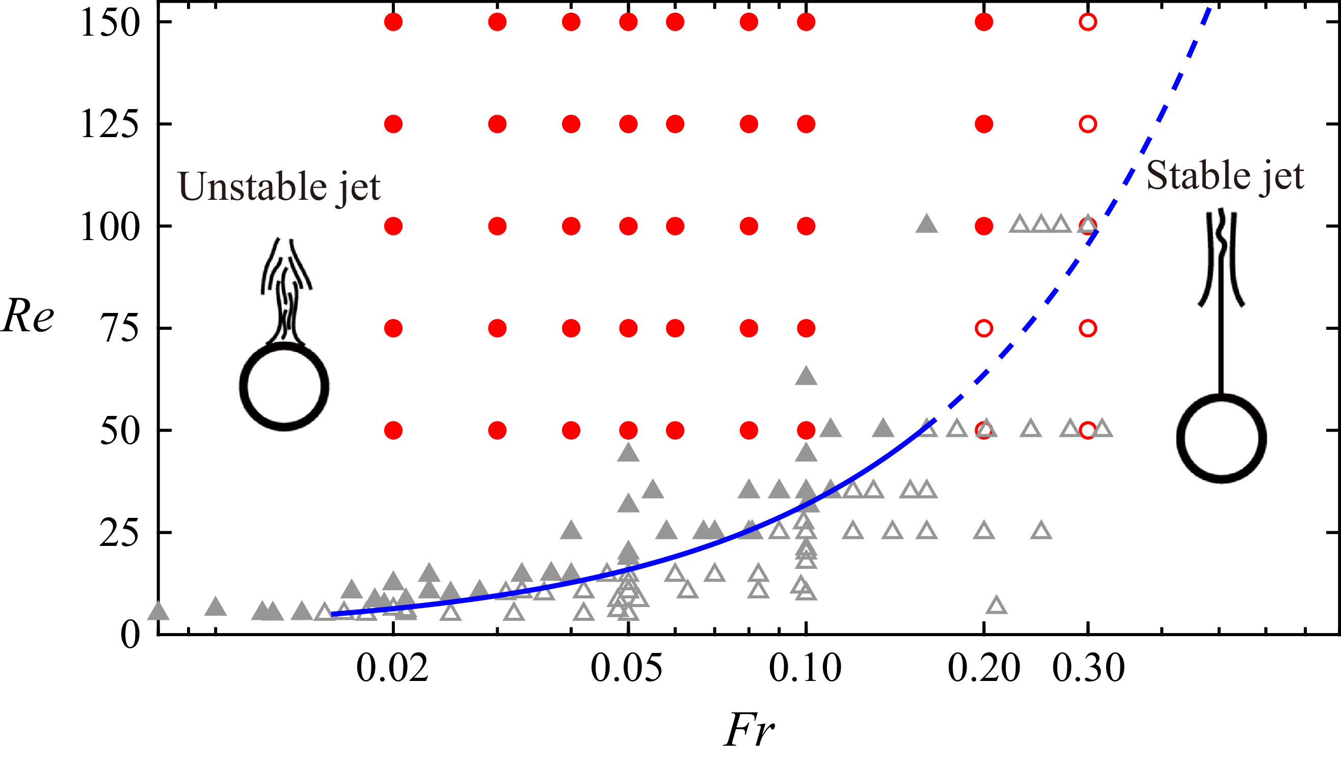
 (Re,Fr)
 Pr=700
 5⩽Re⩽50
 Fr/Re≈3.14×10−3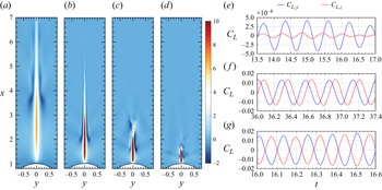
 Fr
Fr Re=100
 Pr=700
 (a−d)
(a−d) (x,y)
(x,y) (a)
(a) Fr=0.3
 (b)
(b) Fr=0.1
 (c)
(c) Fr=0.05
 (d)
(d) Fr=0.02
 (e−g)
(e−g) y
y z
z CL
CL (e)
(e) Fr=0.1
 (f)
(f) Fr=0.05
 (g)
(g) Fr=0.02
 (CL,y,CL,z)
 Re=100
 Pr=700
 (a)
(a) Fr=0.1
 (b)
(b) Fr=0.05
 (c)
(c) Fr=0.02
 (d)
(d) CL,y
CL,y (a−c)
(a−c)
 CLmax
CLmax hxmax
hxmax
 (a−b)
(a−b) Fr=0.05
 t=30
t=30 t=30.1
 (c−d)
(c−d) Fr=0.02
 t=17.09
 t=17.11
 (i)
(i) ωx
ωx ωx=−3
ωx=−3 ωx=+3
ωx=+3 x=1.8
x=1.8 (a−b)
(a−b) x=1.6
x=1.6 (c−d)
(c−d) (ii)
(ii) ωx=±3
ωx=±3 (a−b)
(a−b) ωx=±20
 (c−d)
(c−d) (ux−1)=1.2
 (iii)
(iii) (ii)
(ii)
 (Fr,Re,Pr)=(0.02,100,700)
 (a)
(a) y
y z
z (b)
(b) Kϕ
Kϕ Hmax
Hmax (b)
(b) (x,y)
(x,y) (0⩽|ux−1|<22)
 A,B,C
A,B,C D
D
 (a)
(a) (CL,y,CL,z)
 2
2 (b)
(b) (b)
(b) (ux−1)=1.2
 x=2.1
x=2.1 (c−h)
(c−h) (x,y)
(x,y) (c−h)
(c−h) (ux−1)=1.2
 (ux−1)=−1.4
 (a
(a c)
c) t=2.1
t=2.1 2.2
2.2 2.3
2.3 (d)
(d) (e)
(e) (a−b)
(a−b)
 (a)
(a) y=0.05
 z=0
z=0 (b)
(b) x=1.60
 1.88
1.88 (c)
(c) ρ(x,r,t)−x=const.
 (b)
(b) (c)
(c)
 (a)
(a) (CL,y,CL,z)
 (b)
(b) (ux−1)=1.2
 x=2.1
x=2.1 (c−h)
(c−h) (c−h)
(c−h) 3
3 (a)
(a)
 Fr
Fr (Re,Pr)=(100,700)
 (a)
(a) Fr=0.02
 (b)
(b) Fr=0.05
 (c)
(c) Fr=0.5
 (a)
(a) (CL,y,CL,z)
 (b)
(b) (ux−1)=1.2
 x=2.0
x=2.0 (c−h)
(c−h) (c−h)
(c−h) 6
6
 ux−1
ux−1 (a)
(a) Fr=0.02
 (b)
(b) Fr=0.2
 (a)
(a)
 (a)
(a) (CL,y,CL,z)
 (b)
(b) (ux−1)=1.2
 x=1.5
x=1.5 (c−h)
(c−h) (c−h)
(c−h) 15.95
15.95
 (a)
(a) x=x0
x=x0 ϕ
ϕ x
x (b)
(b) ωr′
ωr′ x
x uϕ′
uϕ′ ϕ
ϕ ux′
ux′ (c)
(c) ω¯ϕ
ω¯ϕ uϕ′
uϕ′ ωx′
ωx′ r
r ϕ
ϕ (d)
(d) ρ′<0
ρ′<0 ∂rρ¯
∂rρ¯ ϕ
ϕ
 t=4
t=4 (Fr,Re,Pr)=(0.02,100,700)
 (a)
(a) x=1.0
x=1.0 0.0065⩽r0⩽0.035
 Δϕ=π/3
 (b)
(b) ∂ru¯x
∂ru¯x (c−h)
(c−h) (x,y)
(x,y) r0
r0 ϕ=0
ϕ=0 π
π r0
r0 (a)
(a) (c−h)
(c−h)
 t=5.95
 (Fr,Re,Pr)=(0.02,100,700)
 (a,i)
(a,i) Tr=r−1(Fr)−2∂ϕρ
 z=0
z=0 (ux−1)=1.2
 (b,i)
(b,i) ωr
ωr (c−I)
(c−I) uϕ
uϕ ux−1=0
 (d−I)
(d−I) ωx=±1
ωx=±1 II
II I
I x=1.8
x=1.8
 (a)
(a) Pr=700
 (b)
(b) Pr=70
Pr=70 (CL,y,CL,z)
 (Fr,Re,Pr)=(0.02,100,700)
 Nξ×Nθ=200×420
 Δξ=Δθ=5.0×10⁻⁴
 (a)
(a) Nϕ=64
Nϕ=64 ξ
ξ θ
θ ϕ
ϕ (b)
(b) Nϕ=32
Nϕ=32 64
64 (c)
(c)
 (Fr,Re,Pr)=(0.02,100,700)
 (a)
(a) (CL,y,CL,z)
 (b)
(b) Δξ=Δθ=5×10⁻⁴
 Δξ=1×10⁻³,Δθ=5×10⁻⁴
 Δξ=5×10⁻⁴,Δθ=1×10⁻³
 Δξ=2.5×10⁻⁴,Δθ=5×10⁻⁴
 (Fr,Re,Pr)=(0.3,100,700)
 ux′=10−2exp{−400[(y−0.005)2+(x−2)2]}
 20
20 ux−1
ux−1 a)
a) t=20
t=20 (b)
(b) t=22
t=22 (c)
(c) t=62
t=62
 (a)
(a) Δϕ
Δϕ r0
r0 ϕ0=0
ϕ0=0 Fr=0.02
 0.05
0.05 0.1
0.1 (b)
(b) Δϕ
Δϕ r0=0.009
 0.014
0.014 0.03
0.03 Fr
Fr (a)
(a)
 Open access

