


1. Introduction
The design of stellarators is a computationally intensive task. The most basic problem in stellarator design – that of computing the magnetic field – requires solving the steady-state magnetohydrostatics (MHS) equations. These equations are difficult to solve for reasons familiar to many problems in physics: they are nonlinear and three-dimensional. Popular MHS equilibrium solvers include VMEC (Hirshman Reference Hirshman1983), DESC (Dudt & Kolemen Reference Dudt and Kolemen2020) and SPEC (Hudson et al. Reference Hudson, Dewar, Dennis, Hole, McGann, von Nessi and Lazerson2012), all of which take seconds to minutes to compute a single equilibrium. Beyond equilibrium solving, there are potentially many other stellarator objectives that are expensive to compute, with plasma stability metrics being a major example. When optimising for stellarators, the costs of equilibrium and objective solving can limit the speed of the overall design process. This, in combination with the high dimensionality of specifying three-dimensional (3-D) fields, motivates a need for simpler alternatives.
Recently, near-axis expansion (Mercier Reference Mercier1964; Solov’ev & Shafranov Reference Solov’ev, Shafranov and Leontovich1970) has gained traction as an alternative to full 3-D MHS solvers. The near-axis expansion works by asymptotically expanding all of the relevant plasma variables (such as magnetic coordinates, pressure, rotational transform and plasma current) in the distance from the magnetic axis, which is assumed to be small relative to a characteristic magnetic scale length. The resulting equations are a hierarchy of one-dimensional ordinary differential equations (ODEs), which can be solved orders of magnitude faster than 3-D equilibria. This allows for one to quickly find large numbers of optimised stellarators (Landreman Reference Landreman2022; Giuliani Reference Giuliani2024), something that was previously unavailable to the stellarator community.
In addition to the speed, the near-axis expansion has other benefits. For instance, Garren & Boozer (Reference Garren and Boozer1991) showed that quasisymmetry imposes more constraints than free parameters in the expansion, leading to the conjecture that non-axisymmetric but perfectly quasisymmetric stellarators cannot exist. Many objectives have been defined and computed for the near-axis expansion, including quasisymmetry (Landreman & Sengupta Reference Landreman and Sengupta2019), quasi-isodynamicity (Mata et al. Reference Mata, Plunk and Jorge2022), isoprominence (Burby et al. Reference Burby, Duignan and Meiss2023), and Mercier and magnetic-well conditions for stability (Landreman & Jorge Reference Landreman and Jorge2020; Kim et al. Reference Kim, Jorge and Dorland2021). There is evidence that other higher-order effects such as ballooning and linear gyrokinetic stability could be investigated as well (Jorge & Landreman Reference Jorge and Landreman2020). The near-axis expansion has also been combined with a type of quadratic flux minimising surfaces and coil optimisation to create free-field optimised quasi-axisymmetric (QA) equilibria (Giuliani Reference Giuliani2024). In sum, the connection among easily expressed objectives, a relatively low-dimensional equilibrium description and fast computation has led to the increased use of the near-axis expansion.
However, the near-axis expansion is not without drawbacks. The primary drawback is fundamental: the expansion has limited accuracy far from the axis. For instance, in the ‘far-axis’ regime, there can be large errors in the magnetic shear and magnetic surfaces can self-intersect (Landreman Reference Landreman2022). The paper by Jorge & Landreman (Reference Jorge and Landreman2020) also indicates that higher-order terms may be needed for stability; such as magnetic curvature terms. Unfortunately, attempts to use higher-order terms have resulted in divergent asymptotic series, limiting the accuracy to small plasma volumes. Most series go to first, second or sometimes third order in the distance from the axis in the relevant quantities, with any more terms typically reducing accuracy rather than improving it. Therefore, if we want to include more physics objectives over larger volumes in the near-axis expansion, we must overcome the issue of series divergence.
Unfortunately, the issue of divergence is confounded by many of the assumptions that can be incorporated into the near-axis expansion. The most extreme case is that of QA stellarators, where it has been shown that the system of equations for quasi-axisymmetry is overdetermined beyond third order in the expansion. Obviously, unless one relaxes the problem (e.g. via anisotropic pressure; Rodríguez & Bhattacharjee Reference Rodríguez and Bhattacharjee2021), one cannot generally ask for a convergent QA near-axis expansion in such a circumstance. In the simpler case of non-quasisymmetric stellarators with smooth pressure gradients and nested surfaces, it is still unknown whether there are non-axisymmetric solutions to MHS (Grad Reference Grad1967; Constantin et al. Reference Constantin, Drivas and Ginsberg2021a ). Recent work has found that perturbing for small force (Constantin et al. Reference Constantin, Drivas and Ginsberg2021b ) or non-flat metrics (Cardona et al. Reference Cardona, Duignan and Perrella2024) allow for integrable solutions, but currently, there is no guarantee of solutions of MHS, let alone convergent asymptotic expansions.
So, to begin the task of building convergent numerical methods for the near-axis expansion, we focus on a problem we know is solvable: Laplace’s equation for vacuum magnetic potentials following Jorge et al. Reference Jorge and Landreman(2020). This can be solved in direct (Mercier) coordinates (Mercier Reference Mercier1964) with no assumption of nested surfaces. Additionally, because solutions of Laplace’s equation are real analytic, there exist near-axis expansions of the equation that converge within a neighbourhood of the axis. Despite these guarantees, even the near-axis expansion of Laplace’s equation diverges.
In this paper, we show that the vacuum near-axis expansion diverges for a reason: Laplace’s equation as a near-axis expansion is ill-posed (§ 3, following background in § 2). To address this issue, we introduce a small regularisation term to Laplace’s equation and expand to find a regularised near-axis expansion. We do this by including a viscosity term to Laplace’s equation that damps the highly oscillatory unstable modes responsible for the ill-posedness. By appropriately bounding the input of the near-axis expansion in a Sobolev norm, we prove that this term results in a uniformly converging near-axis expansion within a neighbourhood of the axis.
Following the theory, we describe a pseudo-spectral method for finding solutions to the near-axis expansion to arbitrary order in § 4. In § 5, we use the numerical method to show two examples of high-order near-axis expansions: the rotating ellipse and Landreman–Paul (Landreman & Paul Reference Landreman and Paul2022). We find that the near-axis expansion magnetic field, rotational transform and magnetic surfaces can converge accurately near the axis for unperturbed initial data. The region of convergence is observed to be dictated by the distance from the magnetic axis to the coils. Then, by perturbing the on-axis inputs, we show that the regularised expansion obeys Laplace’s more accurately farther from the axis. Finally, we conclude in § 6.
2. Background
In this section, we introduce the near-axis expansion for the vacuum field equilibrium problem. This presentation follows closely that of Jorge et al. Reference Jorge and Landreman(2020). We begin with a discussion of the geometry of the near-axis problem (§ 2.1), introduce the near-axis expansion (§ 2.2), define the magnetic field problem (§ 2.3) and finally discuss finding straight field-line magnetic coordinates (§ 2.4). For a fuller discussion of the near-axis expansion to all orders, including with pressure gradients, we recommend the papers by Jorge et al. Reference Jorge and Landreman(2020) and Sengupta et al. Reference Sengupta, Rodriguez, Jorge, Landreman and Bhattacharjee(2024). For ease of reference, we have summarised the equations in the background in box (2.30) for the magnetic field and box (2.60) for magnetic coordinates.
2.1. Near-axis geometry
We define a magnetic axis as a $C^\infty$
closed curve
$C^\infty$
closed curve $\boldsymbol{r}_0 : \mathbb{T} \to \mathbb{R}^3$
with
$\boldsymbol{r}_0 : \mathbb{T} \to \mathbb{R}^3$
with $\boldsymbol{r}_0' \neq 0$
and a non-zero tangent magnetic field (see § 2.3 for details about the field). We define a near-axis domain about the axis with radius
$\boldsymbol{r}_0' \neq 0$
and a non-zero tangent magnetic field (see § 2.3 for details about the field). We define a near-axis domain about the axis with radius $\sigma$
as
$\sigma$
as
 \begin{equation} \Omega _\sigma = \left \{\boldsymbol{r} \in \mathbb{R}^3 \mid \forall s \in \mathbb{T}, \ \left \lVert \boldsymbol{r} - \boldsymbol{r}_0(s) \right \rVert \lt \sigma \right \}. \end{equation}
We note that the assumption that the axis is infinitely differentiable is necessary for the near-axis expansion to formally go to arbitrary order, and we will eventually reduce the required regularity for the inputs of the regularised expansion, summarised in box (3.30).
Schematic of the direct near-axis Frenet–Serret coordinate frame.
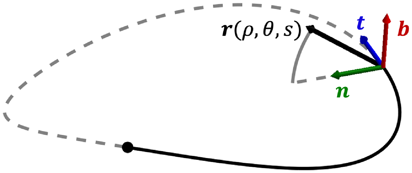
We define a direct coordinate system $\boldsymbol{r} : \Omega _\sigma ^0 \to \Omega _\sigma$
where
$\boldsymbol{r} : \Omega _\sigma ^0 \to \Omega _\sigma$
where $(\rho ,\theta ,s) \in \Omega _\sigma ^0 = [0,\sigma ) \times \mathbb{T}^2$
is the solid torus as (see figure 1)
$(\rho ,\theta ,s) \in \Omega _\sigma ^0 = [0,\sigma ) \times \mathbb{T}^2$
is the solid torus as (see figure 1)
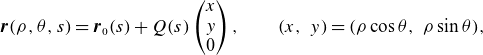 \begin{equation} \boldsymbol{r}(\rho , \theta , s) = \boldsymbol{r}_0(s) + Q(s) \begin{pmatrix} x \\ y \\ 0 \end{pmatrix}, \qquad (x, \ y) = (\rho \cos \theta , \ \rho \sin \theta ), \end{equation}
where $Q$
is an orthonormal basis for the local coordinates at the axis with the tangent vector in the third column, i.e.
$Q$
is an orthonormal basis for the local coordinates at the axis with the tangent vector in the third column, i.e. $\boldsymbol{t} = \boldsymbol{r}_0' / \ell ' = Q\boldsymbol{e}_3$
, where we assume
$\boldsymbol{t} = \boldsymbol{r}_0' / \ell ' = Q\boldsymbol{e}_3$
, where we assume $\ell ' = \left \lVert \boldsymbol r_0' \right \rVert \gt 0$
. Both the
$\ell ' = \left \lVert \boldsymbol r_0' \right \rVert \gt 0$
. Both the $\boldsymbol{x} = (x,y,s)$
and the
$\boldsymbol{x} = (x,y,s)$
and the $\boldsymbol{q} = (\rho , \theta ,s)$
coordinate frames are useful, as
$\boldsymbol{q} = (\rho , \theta ,s)$
coordinate frames are useful, as $\boldsymbol{x}$
is non-singular with respect to the coordinate transformation, while
$\boldsymbol{x}$
is non-singular with respect to the coordinate transformation, while $\boldsymbol{q}$
diagonalises the near-axis expansion operator. To perform calculus in the
$\boldsymbol{q}$
diagonalises the near-axis expansion operator. To perform calculus in the $\boldsymbol{q}$
basis, we require the induced metric from
$\boldsymbol{q}$
basis, we require the induced metric from $\mathbb{R}^3$
. For this, we first compute the coordinate derivative
$\mathbb{R}^3$
. For this, we first compute the coordinate derivative
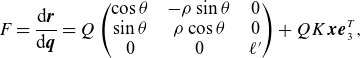 \begin{equation} F = \frac {\mathrm{d} \boldsymbol{r}}{\mathrm{d} \boldsymbol{q}} = Q \left(\begin{array}{c@{\quad}c@{\quad}c} \cos \theta & - \rho \sin \theta & 0\\ \sin \theta & \rho \cos \theta & 0\\ 0 & 0 & \ell ' \end{array}\right) + Q K \boldsymbol{x} \boldsymbol{e}_3^T, \end{equation}
where $K$
is an antisymmetric matrix determining the derivative of
$K$
is an antisymmetric matrix determining the derivative of $Q$
in the near-axis basis
$Q$
in the near-axis basis $Q'(s) = Q K$
. Using this matrix, the metric is computed as
$Q'(s) = Q K$
. Using this matrix, the metric is computed as
 \begin{equation} g = F^T F. \end{equation}
For the numerical examples in this paper, we specifically consider the Frenet–Serret frame, meaning the local basis $Q$
and its derivative are defined by
$Q$
and its derivative are defined by
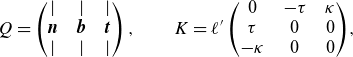 \begin{equation} Q = \left(\begin{array}{c@{\quad}c@{\quad}c} | & | & | \\ \boldsymbol{n} & \boldsymbol{b} & \boldsymbol{t} \\ | & | & | \end{array}\right), \qquad K = \ell ' \left(\begin{array}{c@{\quad}c@{\quad}c} 0 & -\tau & \kappa \\ \tau & 0 & 0 \\ -\kappa & 0 & 0 \end{array}\right)\!, \end{equation}
where $\kappa = \left \lVert \boldsymbol{t}' \right \rVert /\ell '$
is the axis curvature,
$\kappa = \left \lVert \boldsymbol{t}' \right \rVert /\ell '$
is the axis curvature, $\boldsymbol{n} = \left \lVert \boldsymbol{t}' \right \rVert /(\kappa \ell ')$
is the normal vector,
$\boldsymbol{n} = \left \lVert \boldsymbol{t}' \right \rVert /(\kappa \ell ')$
is the normal vector, $\boldsymbol{b} = \boldsymbol{t} \times \boldsymbol{n}$
is the binormal vector and
$\boldsymbol{b} = \boldsymbol{t} \times \boldsymbol{n}$
is the binormal vector and $\tau = -\left \lVert \boldsymbol{b}' \right \rVert /\ell '$
is the axis torsion. Alternative forms of the curvature and torsion are
$\tau = -\left \lVert \boldsymbol{b}' \right \rVert /\ell '$
is the axis torsion. Alternative forms of the curvature and torsion are
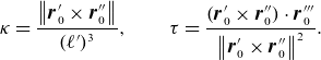 \begin{equation} \kappa = \frac {\left \lVert \boldsymbol{r}_0' \times \boldsymbol{r}_0'' \right \rVert }{(\ell ')^3}, \qquad \tau = \frac {(\boldsymbol{r}_0' \times \boldsymbol{r}_0'') \cdot \boldsymbol{r}_0'''}{\left \lVert \boldsymbol{r}_0' \times \boldsymbol{r}_0'' \right \rVert ^2}. \end{equation}
For the Frenet–Serret coordinate system to be well-defined and non-singular on $\Omega _\sigma ^0$
, we require
$\Omega _\sigma ^0$
, we require $\sigma ^{-1} \gt \kappa \gt 0$
. In particular, no straight segments are allowed in the Frenet–Serret frame, disallowing quasi-isodynamic (QI) stellarators (Mata et al. Reference Mata, Plunk and Jorge2022). An alternative choice for axis coordinates that allow for straight segments is Bishop’s coordinates (Bishop Reference Bishop1975; Duignan & Meiss Reference Duignan and Meiss2021).
$\sigma ^{-1} \gt \kappa \gt 0$
. In particular, no straight segments are allowed in the Frenet–Serret frame, disallowing quasi-isodynamic (QI) stellarators (Mata et al. Reference Mata, Plunk and Jorge2022). An alternative choice for axis coordinates that allow for straight segments is Bishop’s coordinates (Bishop Reference Bishop1975; Duignan & Meiss Reference Duignan and Meiss2021).
Replacing the Frenet–Serret basis into (2.3), we obtain
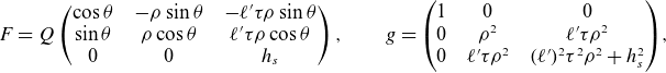 \begin{equation} F = Q \left(\begin{array}{c@{\quad}c@{\quad}c} \cos \theta & - \rho \sin \theta & -\ell ' \tau \rho \sin \theta \\ \sin \theta & \rho \cos \theta & \ell ' \tau \rho \cos \theta \\ 0 & 0 & h_s \end{array}\right),\qquad g = \left(\begin{array}{c@{\quad}c@{\quad}c} 1 & 0 & 0 \\ 0 & \rho ^2 & \ell ' \tau \rho ^2 \\ 0 & \ell ' \tau \rho ^2 & (\ell ')^2\tau ^2 \rho ^2 + h_s^2 \end{array}\right)\!, \end{equation}
where
 \begin{equation} h_s(\rho ,\theta ,s) = \ell ' (1 - \kappa \rho \cos \theta ). \end{equation}
The local volume ratio is given by
 \begin{equation} \sqrt g = \det F = \rho h_s \end{equation}
and the inverse metric is
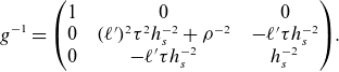 \begin{equation} g^{-1} = \left(\begin{array}{c@{\quad}c@{\quad}c} 1 & 0 & 0 \\ 0 & (\ell ')^2 \tau ^2 h_s^{-2} + \rho ^{-2} & -\ell ' \tau h_s^{-2} \\ 0 & -\ell ' \tau h_s^{-2} & h_s^{-2} \end{array}\right)\!. \end{equation}
To find metrics associated with the more general coordinate system (2.2), we consider transformations of the form $(\rho ,\theta ,s) \mapsto (\rho ,\omega (\theta ,s),s)$
, where
$(\rho ,\theta ,s) \mapsto (\rho ,\omega (\theta ,s),s)$
, where $\omega (\theta ,s) =\theta + \lambda (s)$
. This transformation rotates the orthonormal frame, changing the metric to
$\omega (\theta ,s) =\theta + \lambda (s)$
. This transformation rotates the orthonormal frame, changing the metric to
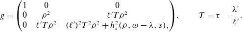 \begin{equation} g = \left(\begin{array}{c@{\quad}c@{\quad}c} 1 & 0 & 0 \\ 0 & \rho ^2 & \ell ' T \rho ^2 \\ 0 & \ell ' T \rho ^2 & (\ell ')^2T^2 \rho ^2 + h_s^2(\rho ,\omega -\lambda ,s), \end{array}\right)\!, \qquad T = \tau - \frac {\lambda '}{\ell '}. \end{equation}
In this way, the general set of near-axis frames can be represented by a simple replacement of $\tau$
with
$\tau$
with $T$
. A special case of this transformation is when
$T$
. A special case of this transformation is when $T=0$
, yielding (Mercier Reference Mercier1964)
$T=0$
, yielding (Mercier Reference Mercier1964)
 \begin{equation} \lambda = \int _{0}^s \tau (s) \ell '(s) \hspace {1pt} \mathrm{d} s. \end{equation}
In this coordinate frame, the metric becomes diagonal: $g = \textrm{Diag}(1, \rho ^2, h_s^2(\rho ,\omega -\lambda ,s))$
. The fact that
$g = \textrm{Diag}(1, \rho ^2, h_s^2(\rho ,\omega -\lambda ,s))$
. The fact that $g$
is diagonalised is convenient for theoretical manipulations, but variables expressed in terms of
$g$
is diagonalised is convenient for theoretical manipulations, but variables expressed in terms of $\omega$
are multivalued for curves with non-integer total torsion. This unfortunate consequence is important for numerical methods, as Fourier series cannot be used in
$\omega$
are multivalued for curves with non-integer total torsion. This unfortunate consequence is important for numerical methods, as Fourier series cannot be used in $s$
and additional consistency requirements are necessary. This is part of the motivation for using the Frenet–Serret frame for the numerical examples herein.
$s$
and additional consistency requirements are necessary. This is part of the motivation for using the Frenet–Serret frame for the numerical examples herein.
2.2. Near-axis expansion
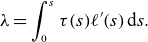
Now, we consider expansions of functions $A \in C^\infty (\Omega _\sigma ^0)$
about the magnetic axis. We formally expand in small distances from the axis
$A \in C^\infty (\Omega _\sigma ^0)$
about the magnetic axis. We formally expand in small distances from the axis $\rho \ll \min \kappa ^{-1}$
as
$\rho \ll \min \kappa ^{-1}$
as
 \begin{gather} A(\rho , \theta , s) = \sum _{m=0}^{\infty }A_m(\theta ,s) \rho ^m, \qquad A_m(\theta , s) = \sum _{n=0}^m A_{mn}(s) e^{(2n-m){\mathrm{i}}\theta }, \nonumber \\ A_{mn}(s) = \sum _{k\in \mathbb{Z}} A_{mnk}e^{{\mathrm{i}} k s}. \end{gather}
This expansion is not guaranteed to converge anywhere for $A\in C^\infty$
, but it is asymptotic to
$A\in C^\infty$
, but it is asymptotic to $A$
near the axis, i.e.
$A$
near the axis, i.e.
 \begin{equation} \left | A - A_{\lt m} \right | = \mathcal{O}(\rho ^{m}), \end{equation}
where we define $A_{\lt m}$
as the partial sum
$A_{\lt m}$
as the partial sum
 \begin{equation} A_{\lt m} = \sum _{n=0}^{m-1} A_n \rho ^n. \end{equation}
In defining magnetic coordinates, we also find it convenient to expand $A$
in
$A$
in $\boldsymbol x$
as
$\boldsymbol x$
as
 \begin{equation} A(x,y,s) = \sum _{\mu =0}^{\infty } \sum _{\nu = 0}^\mu A_{\mu \nu }(s) x^{\mu -\nu } y^\nu , \end{equation}
where we use Latin indices for the $\boldsymbol{q}$
frame and Greek indices for the
$\boldsymbol{q}$
frame and Greek indices for the $\boldsymbol{x}$
frame. If we require
$\boldsymbol{x}$
frame. If we require $A$
to be real-analytic on
$A$
to be real-analytic on $\Omega _\sigma ^0$
, there additionally exists a
$\Omega _\sigma ^0$
, there additionally exists a $\sigma ' \lt \sigma$
so that the the asymptotic series converges uniformly on
$\sigma ' \lt \sigma$
so that the the asymptotic series converges uniformly on $\Omega _{\sigma '}^0$
(this does not necessarily extend to all of
$\Omega _{\sigma '}^0$
(this does not necessarily extend to all of $\Omega _\sigma ^0$
).
$\Omega _\sigma ^0$
).
Throughout this paper, we attempt to minimise the number of complicated summation formulae resulting from the near-axis expansion (NAE). For instance, if we have two functions $A, B\in C^{\infty }$
and we want the
$A, B\in C^{\infty }$
and we want the $m$
th component of the series of
$m$
th component of the series of $C=AB$
, we will write
$C=AB$
, we will write $C_{m} = (AB)_{m}$
, rather than
$C_{m} = (AB)_{m}$
, rather than
 \begin{equation} C_{m} = \sum _{\ell = 0}^m A_{m-\ell } B_\ell . \end{equation}
As expressions become increasingly complicated, this notation provides a concise description of the mathematics involved. In Appendix B, we define a number of relevant operations on series that the interested reader can use to expand the expressions within this paper. In § 4, we discuss how this is similarly convenient for the purposes of programming NAE operations. Rather than implementing residuals via complicated summation formulae, the operations in Appendix B are called, allowing for a simple framework for developing new code.
An important exception to the general rule of condensing notation is in defining any linear operators that must be inverted through the course of an asymptotic expansion. Detailed understanding of such operators are necessary for both numerical implementation and analysis on the series.
2.3. Vacuum fields
In the steady state, the vacuum magnetic field $\boldsymbol{B}\in C^\infty (\Omega _\sigma ^0)$
satisfies
$\boldsymbol{B}\in C^\infty (\Omega _\sigma ^0)$
satisfies
 \begin{equation} \nabla \cdot \boldsymbol{B} = 0, \qquad \boldsymbol{J} = \nabla \times \boldsymbol{B} = 0, \end{equation}
where $\boldsymbol{J}$
is the plasma current density. The fundamental near-axis assumption is that
$\boldsymbol{J}$
is the plasma current density. The fundamental near-axis assumption is that $\boldsymbol{B}$
evaluated on the axis is non-zero and parallel to the magnetic axis, i.e. for some
$\boldsymbol{B}$
evaluated on the axis is non-zero and parallel to the magnetic axis, i.e. for some $B_0 \in C^{\infty }(\mathbb{T})$
,
$B_0 \in C^{\infty }(\mathbb{T})$
,
 \begin{equation} \boldsymbol{B}(0,\theta ,s) = B_0(s) \boldsymbol{t}(s). \end{equation}
Off the axis, we express the magnetic field on $\Omega _\sigma ^0$
as
$\Omega _\sigma ^0$
as
 \begin{equation} \boldsymbol{B} = \nabla \phi + \tilde {\boldsymbol{B}}, \qquad \tilde {\boldsymbol{B}} = \nabla \left [ \int _{0}^s B_0(s') \ell '(s') \hspace {1pt} \mathrm{d} s'\right ] = B_0(s)\ell '(s) \nabla s, \end{equation}
where $\phi \in C^{\infty }(\Omega _\sigma ^0)$
is the magnetic potential satisfying
$\phi \in C^{\infty }(\Omega _\sigma ^0)$
is the magnetic potential satisfying $\left .\nabla \phi \right |_{\rho =0} = 0$
. Then, taking the divergence of (2.20), we find the magnetic scalar potential satisfies Poisson’s equation,
$\left .\nabla \phi \right |_{\rho =0} = 0$
. Then, taking the divergence of (2.20), we find the magnetic scalar potential satisfies Poisson’s equation,
 \begin{equation} \Delta \phi = - \nabla \cdot \tilde {\boldsymbol{B}}. \end{equation}
By construction, the field $\boldsymbol{B}$
in (2.20) is locally the gradient of some function, so it is curl-free. This means the contributions from
$\boldsymbol{B}$
in (2.20) is locally the gradient of some function, so it is curl-free. This means the contributions from $\tilde {\boldsymbol{B}}$
in (2.20) can locally be absorbed to recover Laplace’s equation for the potential. However, because
$\tilde {\boldsymbol{B}}$
in (2.20) can locally be absorbed to recover Laplace’s equation for the potential. However, because $\Omega _\sigma$
is not simply connected and
$\Omega _\sigma$
is not simply connected and $\boldsymbol B \cdot \boldsymbol t$
is single-valued on axis, the closed-loop axis integral
$\boldsymbol B \cdot \boldsymbol t$
is single-valued on axis, the closed-loop axis integral $\oint \boldsymbol{B} \cdot \mathrm{d} \boldsymbol \ell$
demonstrates that it is not possible for
$\oint \boldsymbol{B} \cdot \mathrm{d} \boldsymbol \ell$
demonstrates that it is not possible for $\boldsymbol{B}$
to be globally the gradient of a single-valued function
$\boldsymbol{B}$
to be globally the gradient of a single-valued function $\phi$
. In contrast, the Poisson’s equation formulation contains only single-valued functions, which is convenient both numerically and analytically.
$\phi$
. In contrast, the Poisson’s equation formulation contains only single-valued functions, which is convenient both numerically and analytically.
In coordinates, we can write the magnetic field in (2.20) as
 \begin{equation} B^i = g^{ij} \frac {\partial \phi }{\partial q^j} + \tilde {B}^i, \qquad \tilde {B}^i = B_0 \ell ' g^{ij}\frac {\partial s}{\partial q^j}, \end{equation}
where we assume summation over repeated indices and $g_{ij}$
and
$g_{ij}$
and $g^{ij}$
are the components of the metric and inverse metric, respectively. Then, Poisson’s equation in coordinates becomes
$g^{ij}$
are the components of the metric and inverse metric, respectively. Then, Poisson’s equation in coordinates becomes
 \begin{equation} \sqrt {g}^{-1}\frac {\partial }{\partial q^i}\left ( \sqrt {g} g^{ij} \frac {\partial \phi }{\partial q^j} \right ) = - \sqrt {g}^{-1} \frac {\partial }{\partial q^i}\left (\sqrt {g} \tilde {B}^i \right ). \end{equation}
Multiplying this by $h_s$
and expanding this in the
$h_s$
and expanding this in the $\boldsymbol q$
coordinate system, we have
$\boldsymbol q$
coordinate system, we have
 \begin{align} &\frac {1}{\rho ^2}\left [ \rho \frac {\partial }{\partial \rho }\left (\mathsf{A} \rho \frac {\partial \phi }{\partial \rho } \right )\right . + \left .\frac {\partial }{\partial \theta }\left (\mathsf{B} \frac {\partial \phi }{\partial \theta }\right )\right ] = \nonumber \\ &- \frac {\partial }{\partial \theta }\left ( \mathsf{C} \left ( \frac {\partial \phi }{\partial s} + B_0 \ell '\right ) \right ) - \frac {\partial }{\partial s}\left ( \mathsf{C} \frac {\partial \phi }{\partial \theta } \right ) - \frac {\partial }{\partial s} \left (\mathsf{D} \left (\frac {\partial \phi }{\partial s} + B_0 \ell ' \right ) \right ), \end{align}
where
 \begin{align} \mathsf{A} &= h_s, & \mathsf{B} &= h_s + \rho ^2 h_s^{-1} (\ell ')^2 \tau ^2 , & \mathsf{C} &= -h_s^{-1} \ell ' \tau , & \mathsf{D} &= h_s^{-1}. \end{align}
From here, we can substitute the asymptotic expansions of $\phi$
and the coefficients
$\phi$
and the coefficients $\mathsf{A}$
,
$\mathsf{A}$
, $\mathsf{B}$
,
$\mathsf{B}$
, $\mathsf{C}$
and
$\mathsf{C}$
and $\mathsf{D}$
into (2.24). At each order in
$\mathsf{D}$
into (2.24). At each order in $\rho$
, Poisson’s equation becomes
$\rho$
, Poisson’s equation becomes
 \begin{align} \ell ' \left (m^2 + \frac {\partial ^2}{\partial \theta ^2}\right ) \phi _{m} =& - (\nabla \cdot \tilde {B})_{m-2} -(\Delta \phi _{\lt m})_{m-2}\nonumber \\ =&- m(m-1) \mathsf{A}_1 \phi _{m-1} - \left [\frac {\partial }{\partial \theta }\left (\mathsf{B} \frac {\partial \phi _{\lt m}}{\partial \theta } \right )\right ]_m \nonumber \\ &- \left [ \frac {\partial }{\partial \theta }\left ( \mathsf{C} \left (\frac {\partial \phi _{\lt m}}{\partial s} + B_0 \ell ' \right ) \right ) + \frac {\partial }{\partial s}\left ( \mathsf{C} \frac {\partial \phi _{\lt m}}{\partial \theta } \right )\right ]_{m-2} \\ \nonumber &- \left [\frac {\partial }{\partial s} \left (\mathsf{D} \left ( \frac {\partial \phi _{\lt m}}{\partial s} + B_0 \ell '\right ) \right )\right ]_{m-2}, \end{align}
where $\mathsf{A}_1 = (h_s)_1 = -\ell ' \kappa \cos \theta$
. The right-hand side of (2.26) does not depend on orders of
$\mathsf{A}_1 = (h_s)_1 = -\ell ' \kappa \cos \theta$
. The right-hand side of (2.26) does not depend on orders of $\phi$
higher than
$\phi$
higher than $\phi _{m-1}$
, so inverting the left-hand-side operator gives an iteration for obtaining
$\phi _{m-1}$
, so inverting the left-hand-side operator gives an iteration for obtaining $\phi _m$
at each order.
$\phi _m$
at each order.
However, the operator $\ell ' (m^2 + ({\partial ^2}/{\partial \theta ^2)})$
is singular, so we must confirm there are no secular terms. Specifically, we always have an unknown homogeneous solution at
$\ell ' (m^2 + ({\partial ^2}/{\partial \theta ^2)})$
is singular, so we must confirm there are no secular terms. Specifically, we always have an unknown homogeneous solution at $\mathcal{O}(m)$
of the form
$\mathcal{O}(m)$
of the form $\phi _{m0} e^{-i m \theta } + \phi _{mm} e^{i m \theta }$
. For this, we use Fredholm’s alternative, which states that (2.26) is solvable if the right-hand side is orthogonal to the null space of the adjoint of the operator on the left-hand side. Because the operator is self-adjoint, the right-hand side must be orthogonal to
$\phi _{m0} e^{-i m \theta } + \phi _{mm} e^{i m \theta }$
. For this, we use Fredholm’s alternative, which states that (2.26) is solvable if the right-hand side is orthogonal to the null space of the adjoint of the operator on the left-hand side. Because the operator is self-adjoint, the right-hand side must be orthogonal to $e^{\pm i m \theta }$
, i.e.
$e^{\pm i m \theta }$
, i.e.
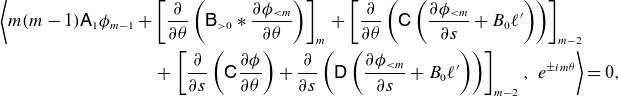 \begin{align} &\left \langle m(m-1) \mathsf{A}_1 \phi _{m-1} + \left [\frac {\partial }{\partial \theta }\left (\mathsf{B}_{\gt 0} * \frac {\partial \phi _{\lt m}}{\partial \theta } \right )\right ]_m \right . + \left [ \frac {\partial }{\partial \theta }\left ( \mathsf{C} \left ( \frac {\partial \phi _{\lt m}}{\partial s} + B_0 \ell '\right ) \right )\right ]_{m-2}\nonumber \\ &\qquad\qquad\qquad\quad\quad\,\,\,+ \left .\left [\frac {\partial }{\partial s}\left ( \mathsf{C} \frac {\partial \phi }{\partial \theta } \right ) + \frac {\partial }{\partial s} \left (\mathsf{D} \left ( \frac {\partial \phi _{\lt m}}{\partial s} + B_0 \ell '\right ) \right )\right ]_{m-2}, \ e^{\pm i m \theta }\right \rangle =0, \end{align}
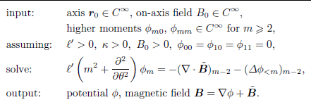
where the inner product is defined by
 \begin{equation} \left \langle f , \ g \right \rangle = \int _{0}^{2\pi } f(\theta )\overline {g}(\theta ) \hspace {1pt} \mathrm{d} \theta . \end{equation}
The $m-2$
coefficient of any analytic function is orthogonal to
$m-2$
coefficient of any analytic function is orthogonal to $e^{i m \theta }$
, so we can remove the
$e^{i m \theta }$
, so we can remove the $\mathsf{C}$
and
$\mathsf{C}$
and $\mathsf{D}$
terms. The same argument allows us to remove the torsion terms in
$\mathsf{D}$
terms. The same argument allows us to remove the torsion terms in $\mathsf{B}$
. This means only contributions from
$\mathsf{B}$
. This means only contributions from $\mathsf{A}_1 = \mathsf{B}_1 = - \ell ' \kappa \cos \theta$
and
$\mathsf{A}_1 = \mathsf{B}_1 = - \ell ' \kappa \cos \theta$
and $\phi _{m-1}$
survive, so we only need to verify
$\phi _{m-1}$
survive, so we only need to verify
 \begin{align} \left \langle m(m-1) \phi _{m-1} \cos \theta + \left [\frac {\partial }{\partial \theta }\left (\frac {\partial \phi _{m-1}}{\partial \theta } \cos \theta \right )\right ]_m , \ e^{\pm i m \theta } \right \rangle = 0. \end{align}
Using the identity $\cos \theta = (e^{i \theta } + e^{-i \theta })/2$
, a quick calculation confirms the above identity holds.
$\cos \theta = (e^{i \theta } + e^{-i \theta })/2$
, a quick calculation confirms the above identity holds.
Now, we consider the problem where $\phi$
is unknown. The fact that the Fredholm condition is automatically satisfied at each order implies that
$\phi$
is unknown. The fact that the Fredholm condition is automatically satisfied at each order implies that $\phi _{m0}$
and
$\phi _{m0}$
and $\phi _{mm}$
are free parameters at each order in the near-axis expansion. So, these coefficients are an infinite-dimensional set of initial conditions for the near-axis expansion of Poisson’s equation. Intuitively, one can think of the coefficients
$\phi _{mm}$
are free parameters at each order in the near-axis expansion. So, these coefficients are an infinite-dimensional set of initial conditions for the near-axis expansion of Poisson’s equation. Intuitively, one can think of the coefficients $\phi _{m0}$
and
$\phi _{m0}$
and $\phi _{mm}$
as specifying the Fourier coefficients of an infinitely thin tube about the magnetic axis. In this way, the imposition of conditions at each order compensates for the fact that partial differential equations (PDEs) typically satisfy conditions on co-dimension-1 surfaces, whereas the near-axis expansion is specified on a co-dimension-2 curve.
$\phi _{mm}$
as specifying the Fourier coefficients of an infinitely thin tube about the magnetic axis. In this way, the imposition of conditions at each order compensates for the fact that partial differential equations (PDEs) typically satisfy conditions on co-dimension-1 surfaces, whereas the near-axis expansion is specified on a co-dimension-2 curve.
In addition to $\phi _{m0}$
and
$\phi _{m0}$
and $\phi _{mm}$
as free parameters, we also treat
$\phi _{mm}$
as free parameters, we also treat $\boldsymbol{r}_0$
and
$\boldsymbol{r}_0$
and $B_0$
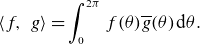
as inputs to the near-axis problem. The requirement that the magnetic field be tangent to the axis with magnitude
$B_0$
as inputs to the near-axis problem. The requirement that the magnetic field be tangent to the axis with magnitude $B_0$
results in a constraint that
$B_0$
results in a constraint that $\phi _{00} = \phi _{10} = \phi _{11} = 0$
. In total, the direct vacuum near-axis problem can be written as
$\phi _{00} = \phi _{10} = \phi _{11} = 0$
. In total, the direct vacuum near-axis problem can be written as
2.4. Straight field-line coordinates: leading order
Given a solution magnetic field from box (2.30), we consider the problem of finding straight field-line magnetic coordinates. We assume that the magnetic field is locally elliptic about the axis and the rotation number is irrational, so that the leading-order behaviour is rotation about the magnetic axis. This means that both hyperbolic orbits (x-points) and on-axis resonant perturbations are excluded from this work. In the language of Hamiltonian normal forms, the leading order field-line dynamics is conjugate to a non-resonant harmonic oscillator; see Burby et al. Reference Burby, Duignan and Meiss(2021) and Duignan & Meiss (Reference Duignan and Meiss2021) for a more rigorous derivation of magnetic coordinates in the near-axis expansion. We note that our process of finding coordinates is formal: we make no claims that this problem converges in the limit. However, in § 5, we find that this procedure appears to converge well numerically.
To find magnetic coordinates, we attempt to build a conjugacy between magnetic field-line dynamics $\dot {\boldsymbol{r}} = (B^s)^{-1} \boldsymbol{B}(\boldsymbol{r})$
and straight field-line dynamics
$\dot {\boldsymbol{r}} = (B^s)^{-1} \boldsymbol{B}(\boldsymbol{r})$
and straight field-line dynamics $\dot {\boldsymbol{\xi }} = (- \iota (\psi ) \eta , \, \iota (\psi ) \xi , \, 1)$
, where
$\dot {\boldsymbol{\xi }} = (- \iota (\psi ) \eta , \, \iota (\psi ) \xi , \, 1)$
, where $\boldsymbol{\xi } = (\xi , \, \eta , \, s) \in \mathbb{R}^2 \times \mathbb{T}$
are Cartesian coordinates,
$\boldsymbol{\xi } = (\xi , \, \eta , \, s) \in \mathbb{R}^2 \times \mathbb{T}$
are Cartesian coordinates, $\psi =\xi ^2 + \eta ^2$
is a flux-like coordinate and
$\psi =\xi ^2 + \eta ^2$
is a flux-like coordinate and $\iota$
is the rotational transform. To make the connection with straight field-line coordinates precise, consider the transformation to polar coordinates
$\iota$
is the rotational transform. To make the connection with straight field-line coordinates precise, consider the transformation to polar coordinates $(\xi , \eta ) \to \sqrt {\psi }(\cos \gamma , \sin \gamma )$
. Then, the field-line is traced by
$(\xi , \eta ) \to \sqrt {\psi }(\cos \gamma , \sin \gamma )$
. Then, the field-line is traced by $(\dot {\psi },\, \dot {\gamma },\, \dot {s}) = (0, \, \iota (\psi ), \, 1)$
, i.e. magnetic field lines are straight with slope
$(\dot {\psi },\, \dot {\gamma },\, \dot {s}) = (0, \, \iota (\psi ), \, 1)$
, i.e. magnetic field lines are straight with slope $\iota$
. However, we use the Cartesian version of magnetic coordinates because it removes the coordinate singularity associated with polar coordinates, simplifying the following steps.
$\iota$
. However, we use the Cartesian version of magnetic coordinates because it removes the coordinate singularity associated with polar coordinates, simplifying the following steps.
A schematic of the process of finding straight field-line coordinates. On the left, we plot the surfaces of the magnetic field $(h^x,h^y)$
on a cross-section for fixed
$(h^x,h^y)$
on a cross-section for fixed $s$
. Moving one plot to the right, the leading correction transforms to a coordinate frame where the main elliptic component is eliminated. Going one further, the next correction accounts for the most prominent triangularity. This process continues until, in
$s$
. Moving one plot to the right, the leading correction transforms to a coordinate frame where the main elliptic component is eliminated. Going one further, the next correction accounts for the most prominent triangularity. This process continues until, in $(\xi ,\eta )$
coordinates, the magnetic surfaces are nested circles.
$(\xi ,\eta )$
coordinates, the magnetic surfaces are nested circles.
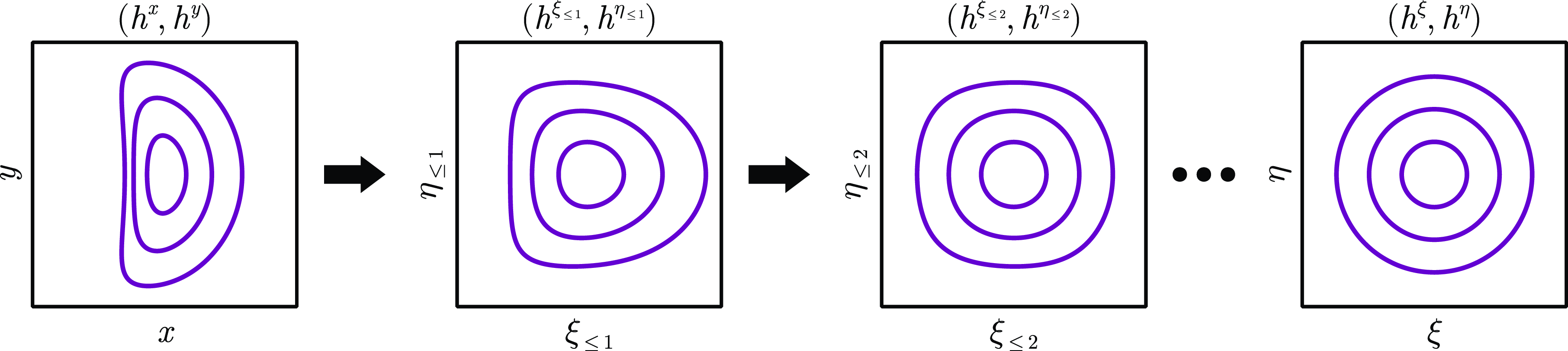
There are two main steps to our process of finding magnetic coordinates: the leading-order problem and the higher-order problems (see figure 2 for a sketch of the process). If we use the notation $\tilde {\boldsymbol{x}} = (x,\, y)$
and
$\tilde {\boldsymbol{x}} = (x,\, y)$
and $\tilde {\boldsymbol{\xi }} = (\xi , \, \eta )$
for the out-of-plane coordinates, the leading order transformation takes the form
$\tilde {\boldsymbol{\xi }} = (\xi , \, \eta )$
for the out-of-plane coordinates, the leading order transformation takes the form
 \begin{equation} \tilde {\boldsymbol{\xi }}_1 = \frac {\partial \tilde {\boldsymbol{\xi }}_1}{\partial \tilde {\boldsymbol{x}}}\tilde {\boldsymbol{x}} = G_0 \tilde {\boldsymbol{x}} = \begin{pmatrix} \xi _{10} x + \xi _{11} y \\ \eta _{10} x + \eta _{11} y \end{pmatrix}. \end{equation}
We will find that the problem for $G_0$
is an eigenvalue problem for the on-axis rotation number, as is typical for the linearised dynamics about a fixed point. In the following section, we will discuss the inductive step to higher orders.
$G_0$
is an eigenvalue problem for the on-axis rotation number, as is typical for the linearised dynamics about a fixed point. In the following section, we will discuss the inductive step to higher orders.
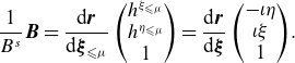
To begin, consider the contravariant form of the Cartesian near-axis magnetic field
 \begin{equation} \frac {1}{B^s} \boldsymbol B = \frac {1}{B^s} \frac {\mathrm{d} \boldsymbol{r}}{\mathrm{d} \boldsymbol{x}} \begin{pmatrix} B^x \\ B^y \\ B^s \end{pmatrix} = \frac {B^x}{B^s} \frac {\partial \boldsymbol{r}}{\partial x} + \frac {B^y}{B^s} \frac {\partial \boldsymbol{r}}{\partial y} + \frac {\partial \boldsymbol{r}}{\partial s}. \end{equation}
We would like to equate this to the straight field-line dynamics as
 \begin{equation} \frac {1}{B^s} \boldsymbol{B} = \frac {\mathrm{d} \boldsymbol{r}}{\mathrm{d} \boldsymbol{\xi }} \begin{pmatrix} - \iota (\psi ) \eta \\ \iota (\psi ) \xi \\ 1 \end{pmatrix}, \end{equation}
where $\iota$
depends smoothly upon the radial label as
$\iota$
depends smoothly upon the radial label as
 \begin{equation} \iota = \iota _0 + \iota _2 \psi + \iota _4\psi ^2 + \ldots , \end{equation}
where we emphasise $\iota _\mu = 0$
for odd
$\iota _\mu = 0$
for odd $\mu$
. Multiplying both sides by
$\mu$
. Multiplying both sides by $\mathrm{d} \boldsymbol{\xi } / \mathrm{d} \boldsymbol{r}$
, we find the Floquet conjugacy problem
$\mathrm{d} \boldsymbol{\xi } / \mathrm{d} \boldsymbol{r}$
, we find the Floquet conjugacy problem
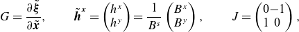
 \begin{equation} \frac {\partial \tilde {\boldsymbol{\xi }}}{\partial s} = -G(\boldsymbol{\xi }) \tilde {\boldsymbol{h}}^{\boldsymbol{x}} +\iota (\psi (\boldsymbol{\xi })) J \tilde {\boldsymbol{\xi }}, \end{equation}
where
 \begin{equation} G = \frac {\partial \tilde {\boldsymbol{\xi }}}{\partial \tilde {\boldsymbol{x}}}, \qquad \tilde {\boldsymbol{h}}^{\boldsymbol{x}} = \begin{pmatrix} h^x \\ h^y \end{pmatrix} = \frac {1}{B^s} \begin{pmatrix} B^x \\ B^y \end{pmatrix}, \qquad J = \begin{pmatrix} 0 & -1 \\ 1 & 0 \end{pmatrix}, \end{equation}
where $J$
is known as the symplectic matrix. Our problem is to solve (2.35) for
$J$
is known as the symplectic matrix. Our problem is to solve (2.35) for $\xi (x,y)$
,
$\xi (x,y)$
, $\eta (x,y)$
and
$\eta (x,y)$
and $\iota (\psi )$
.
$\iota (\psi )$
.
To find the leading-order problem for (2.35), we note the magnetic field $(h^x,h^y)$
is linear at leading order:
$(h^x,h^y)$
is linear at leading order:
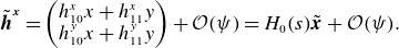 \begin{equation} \tilde {\boldsymbol{h}}^{\boldsymbol{x}} = \begin{pmatrix} h^x_{10} x + h^x_{11} y \\ h^y_{10} x + h^y_{11} y \end{pmatrix} + \mathcal{O}(\psi ) = H_0(s) \tilde {\boldsymbol{x}} + \mathcal{O}(\psi ). \end{equation}
Substituting this, (2.31) and $\iota = \iota _0 + \mathcal{O}(\psi )$
into (2.35), we have
$\iota = \iota _0 + \mathcal{O}(\psi )$
into (2.35), we have
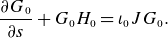 \begin{equation} \frac {\partial G_0}{\partial s} + G_0 H_0 = \iota _0 J G_0. \end{equation}
The leading order problem (2.38) is a Floquet eigenvalue problem for the linearised field-line dynamics about the magnetic axis. Assuming that the near-axis expansion is elliptic at leading order, the value of $\iota _0$
is real. Otherwise,
$\iota _0$
is real. Otherwise, $\iota _0$
is not real, meaning ellipticity can be numerically verified for a given input.
$\iota _0$
is not real, meaning ellipticity can be numerically verified for a given input.
There are many equivalent solutions to (2.38), owing to the symmetries that if $(G_0, \iota _0)$
satisfies (2.38), then the following are also solutions:
$(G_0, \iota _0)$
satisfies (2.38), then the following are also solutions:
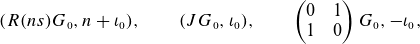 \begin{align} (R(ns) G_0, n + \iota _0), \qquad (J G_0, \iota _0), \qquad \left (\begin{array}{l@{\quad}c} 0 & 1 \\ 1 & 0 \end{array}\right) G_0, -\iota _0, \end{align}
where $R$
is a rotation matrix
$R$
is a rotation matrix
 \begin{equation} R(\theta ) = \left(\begin{array}{l@{\quad}c} \cos \theta & - \sin \theta \\ \sin \theta & \cos \theta \end{array}\right)\!. \end{equation}
The question of which solution to choose is then a question of practicalities. For instance, one could choose the rotational transform corresponding to a non-twisting right-handed coordinate frame $\boldsymbol{\xi }_{1}$
. Here, ‘non-twisting’ means that closed coordinate lines near the axis, implicitly defined as curves
$\boldsymbol{\xi }_{1}$
. Here, ‘non-twisting’ means that closed coordinate lines near the axis, implicitly defined as curves $\boldsymbol r(x,y,s)$
where
$\boldsymbol r(x,y,s)$
where $\tilde {\boldsymbol{\xi }}(x,y,s) \neq 0$
is held constant, can be continuously deformed to a point on
$\tilde {\boldsymbol{\xi }}(x,y,s) \neq 0$
is held constant, can be continuously deformed to a point on $\mathbb{R}^3 \backslash \boldsymbol r_0$
. In other words, the coordinates lines do not link with the axis. In this frame,
$\mathbb{R}^3 \backslash \boldsymbol r_0$
. In other words, the coordinates lines do not link with the axis. In this frame, $\iota _0$
agrees with the intuitive definition of the rotational transform as the limiting ratio of poloidal turns divided by toroidal turns of fieldlines about the axis. Other choices may have other benefits, e.g. there may be an eigenfunction that
$\iota _0$
agrees with the intuitive definition of the rotational transform as the limiting ratio of poloidal turns divided by toroidal turns of fieldlines about the axis. Other choices may have other benefits, e.g. there may be an eigenfunction that $G_0$
behaves best numerically. In this paper, we opt for an option that is easy to implement: we take the real solution where
$G_0$
behaves best numerically. In this paper, we opt for an option that is easy to implement: we take the real solution where $\iota _0$
has the smallest magnitude and
$\iota _0$
has the smallest magnitude and $\det G_0$
is positive. From here, other equivalent coordinates can easily be found by applying the transformations in (2.39).
$\det G_0$
is positive. From here, other equivalent coordinates can easily be found by applying the transformations in (2.39).
For the scaling of $G_0$
, we choose
$G_0$
, we choose $\psi$
to be the actual magnetic flux at leading order. The formula for the flux is
$\psi$
to be the actual magnetic flux at leading order. The formula for the flux is
 \begin{equation} \psi = \int _{\boldsymbol{r}(D_\psi , 0)} \boldsymbol{B} \cdot \boldsymbol{t} \hspace {1pt} \mathrm{d} A = \int _{\boldsymbol{r}(D_\psi , 0)} B_s \hspace {1pt} \mathrm{d} A(\boldsymbol{r}), \end{equation}
where $D_\psi = \{(\xi ,\eta ) \mid \xi ^2 + \eta ^2 \lt \psi \}$
and
$D_\psi = \{(\xi ,\eta ) \mid \xi ^2 + \eta ^2 \lt \psi \}$
and
 \begin{equation} B_s = g_{sj} B^j = \frac {\partial \phi }{\partial s} + B_0 \ell '. \end{equation}
Pulling this back to the $\boldsymbol{\xi }$
frame, we have
$\boldsymbol{\xi }$
frame, we have
 \begin{equation} \psi = \int _{D_\psi }B_s(\boldsymbol{x}(\boldsymbol{\xi }, s), 0) (\det G)^{-1} \hspace {1pt} \mathrm{d} A(\boldsymbol{\xi }). \end{equation}
Both $B_s$
and
$B_s$
and $G_0$
are constant in
$G_0$
are constant in $\boldsymbol{\xi }$
to leading order, so (2.43) at leading order becomes
$\boldsymbol{\xi }$
to leading order, so (2.43) at leading order becomes
 \begin{equation} \int _{D_\psi }B_s(\boldsymbol{x}(\boldsymbol{\xi }, s), 0) (\det G)^{-1} \hspace {1pt} \mathrm{d} A(\boldsymbol{\xi }) = \frac {(B_{s})_0}{\det G_0} \pi \psi + \mathcal{O}(\psi ^2). \end{equation}
Setting this equal to $\psi$
, we find
$\psi$
, we find
 \begin{equation} \det G_0 = \pi (B_s)_0, \end{equation}
where we note that this is only possible when $(B_s)_0$
is chosen to be positive.
$(B_s)_0$
is chosen to be positive.
2.5. Straight field-line coordinates: higher order
Now that we have the leading-order behaviour, we iterate to go to higher order. To do so, first define the near-axis expansion of $\tilde {\boldsymbol{\xi }}$
near the axis as
$\tilde {\boldsymbol{\xi }}$
near the axis as
 \begin{equation} \tilde {\boldsymbol{\xi }} = \sum _{\mu =1}^\infty \tilde {\boldsymbol{\xi }}_\mu (\tilde {\boldsymbol{x}}, s), \qquad \tilde {\boldsymbol{\xi }}_\mu = \sum _{\nu = 0}^\mu \tilde {\boldsymbol{\xi }}_{\mu \nu }(s) x^{\mu -\nu } y^\nu , \end{equation}
and define the partial sums as
 \begin{equation} \tilde {\boldsymbol{\xi }}_{\leqslant \mu } = \sum _{\mu ' = 1}^{\mu }\tilde {\boldsymbol{\xi }}_{\mu '}, \end{equation}
where at leading order, $\tilde {\boldsymbol{\xi }}_{\leqslant 1} = \tilde {\boldsymbol{\xi }}_1 = G_0 \tilde {\boldsymbol{x}}.$
At each order in the iteration, we consider the update to be a function of the previous coordinates, i.e.
 \begin{align} \tilde {\boldsymbol{\xi }}_{\leqslant \mu +1}\Big(\xi _{\leqslant \mu }, \eta _{\leqslant \mu }, s_{\leqslant \mu }\Big) &= \tilde {\boldsymbol{\xi }}_{\leqslant \mu } + \sum _{\nu =0}^\mu \tilde {\boldsymbol{\xi }}_{\mu \nu }\Big(s_{\leqslant \mu }\Big) \xi _{\leqslant \mu }^{\mu -\nu } \eta _{\leqslant \mu }^\nu \nonumber,\\ &= \tilde {\boldsymbol{\xi }}_{\leqslant \mu } + \sum _{\nu =0}^\mu \tilde {\boldsymbol{\xi }}_{\mu \nu } \xi _{1}^{\mu -\nu } \eta _{1}^\nu + \mathcal{O}\Big(\psi ^{(\mu +2)/2}\Big). \end{align}
We explicitly write the transformed toroidal coordinate $s_{\leqslant \mu }=s$
so that it is clear that
$s_{\leqslant \mu }=s$
so that it is clear that $({\partial }/{\partial s})$
and
$({\partial }/{\partial s})$
and $({\partial }/{\partial s_{\leqslant \mu })}$
are different operators. The purpose of performing the update in this way is primarily to make the update step as clear as possible.
$({\partial }/{\partial s_{\leqslant \mu })}$
are different operators. The purpose of performing the update in this way is primarily to make the update step as clear as possible.
To wit, the magnetic field in the new frame satisfies
 \begin{equation} \frac {1}{B^s} \boldsymbol{B} = \frac {\mathrm{d} \boldsymbol{r}}{\mathrm{d} \boldsymbol{\xi }_{\leqslant \mu }} \begin{pmatrix} h^{\xi _{\leqslant \mu }} \\ h^{\eta _{\leqslant \mu }} \\ 1 \end{pmatrix} = \frac {\mathrm{d} \boldsymbol{r}}{\mathrm{d} \boldsymbol{\xi }} \begin{pmatrix} -\iota \eta \\ \iota \xi \\ 1 \end{pmatrix}\!. \end{equation}
We can use the first equality to write
 \begin{align} \tilde {\boldsymbol{h}}^{\boldsymbol{\xi }_{\leqslant \mu }}(\boldsymbol{\xi }_{\leqslant \mu }) &= \begin{pmatrix} h^{\xi _{\leqslant \mu }} \big(\boldsymbol{\xi }_{\leqslant \mu }\big) \\[2pt] h^{\eta _{\leqslant \mu }} \big(\boldsymbol{\xi }_{\leqslant \mu }\big) \end{pmatrix} \nonumber \\ &= \frac {\partial \tilde {\boldsymbol{\xi }}_{\leqslant \mu }}{\partial \tilde {\boldsymbol{x}}} \tilde {\boldsymbol{h}}^{\boldsymbol{x}}\left(\boldsymbol{x}\big(\boldsymbol{\xi }_{\leqslant \mu }\big)\right) + \frac {\partial \tilde {\boldsymbol{\xi }}_{\leqslant \mu }}{\partial s}, \end{align}
 \begin{align} &= [\iota (\psi ) J \tilde {\boldsymbol{\xi }}]_{\leqslant \mu } + \left [ \frac {\partial \tilde {\boldsymbol{\xi }}_{\leqslant \mu }}{\partial \tilde {\boldsymbol{x}}}\tilde {\boldsymbol{h}}^{\boldsymbol{x}}(\boldsymbol{x}(\boldsymbol{\xi }_{\leqslant \mu }))\right ]_{\gt \mu }\!,\\[6pt] \nonumber\end{align}
where we use the notation $f_{\gt \mu } = \sum _{\nu \gt \mu } f_{\nu }$
. To get from the second to the third line, we have used the inductive assumption that
$f_{\gt \mu } = \sum _{\nu \gt \mu } f_{\nu }$
. To get from the second to the third line, we have used the inductive assumption that $\boldsymbol{\xi }_{\leqslant \mu }$
matches
$\boldsymbol{\xi }_{\leqslant \mu }$
matches $\boldsymbol{\xi }$
up to order
$\boldsymbol{\xi }$
up to order $\mu$
, meaning that
$\mu$
, meaning that $\boldsymbol{\xi }_{\leqslant \mu }$
is a straight field-line coordinate system up to order
$\boldsymbol{\xi }_{\leqslant \mu }$
is a straight field-line coordinate system up to order $\mu$
. In this way, we will find that the update residual depends neatly upon the transformed magnetic field.
$\mu$
. In this way, we will find that the update residual depends neatly upon the transformed magnetic field.
It is worth noting that (2.51) has two new operations that have not been introduced so far. The first is that we are computing $\boldsymbol{x}(\boldsymbol{\xi }_{\leqslant \mu })$
, i.e. we are inverting the coordinate transformation. The second is that we are composing functions with this inversion as
$\boldsymbol{x}(\boldsymbol{\xi }_{\leqslant \mu })$
, i.e. we are inverting the coordinate transformation. The second is that we are composing functions with this inversion as $\tilde {\boldsymbol{h}}^{\boldsymbol{x}}(\boldsymbol{x}(\boldsymbol{\xi }_{\leqslant \mu }))$
. So, for any function
$\tilde {\boldsymbol{h}}^{\boldsymbol{x}}(\boldsymbol{x}(\boldsymbol{\xi }_{\leqslant \mu }))$
. So, for any function $f(\boldsymbol{x})$
and coordinate transformation
$f(\boldsymbol{x})$
and coordinate transformation $\boldsymbol{\xi }(\boldsymbol{x})$
, we can compute the equivalent function in indirect coordinates as
$\boldsymbol{\xi }(\boldsymbol{x})$
, we can compute the equivalent function in indirect coordinates as $f(\boldsymbol{\xi })$
using these two steps. Moreover, the inverse transformation
$f(\boldsymbol{\xi })$
using these two steps. Moreover, the inverse transformation $\boldsymbol{x}(\boldsymbol{\xi })$
can be precomputed for all transformations one wishes to perform of this type. This gives a framework to move back and forth between direct and indirect near-axis formalisms to high order. For more details on how these transformations are computed, see Appendices (B.6) and (B.7).
$\boldsymbol{x}(\boldsymbol{\xi })$
can be precomputed for all transformations one wishes to perform of this type. This gives a framework to move back and forth between direct and indirect near-axis formalisms to high order. For more details on how these transformations are computed, see Appendices (B.6) and (B.7).
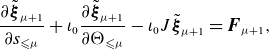
Given the residual field (2.51), we can use the second equality in (2.49) to find the updated equation
 \begin{equation} \frac {\partial \tilde {\boldsymbol{\xi }}}{\partial s_{\leqslant \mu }} = - \frac {\partial \tilde {\boldsymbol{\xi }}}{\partial \tilde {\boldsymbol{\xi }}_{\leqslant \mu }} \tilde {\boldsymbol{h}}^{\boldsymbol{\xi }_{\leqslant \mu }}\big(\boldsymbol{\xi }_{\leqslant \mu }\big) + \iota (\psi ) J \tilde {\boldsymbol{\xi }}. \end{equation}
Note that this has the exact same form as (2.35), except we have shifted the underlying coordinates. Substituting $\tilde {\boldsymbol{\xi }}_{\leqslant \mu +1} = \tilde {\boldsymbol{\xi }}_{\leqslant \mu } + \tilde {\boldsymbol{\xi }}_\mu$
into (2.52), we obtain
$\tilde {\boldsymbol{\xi }}_{\leqslant \mu +1} = \tilde {\boldsymbol{\xi }}_{\leqslant \mu } + \tilde {\boldsymbol{\xi }}_\mu$
into (2.52), we obtain
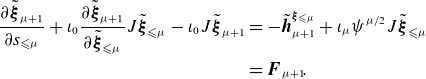 \begin{align} \frac {\partial \tilde {\boldsymbol{\xi }}_{\mu +1}}{\partial s_{\leqslant \mu }} + \iota _0 \frac {\partial \tilde {\boldsymbol{\xi }}_{\mu +1}}{\partial \tilde {\boldsymbol{\xi }}_{\leqslant \mu }} J \tilde {\boldsymbol{\xi }}_{\leqslant \mu } - \iota _0 J \tilde {\boldsymbol{\xi }}_{\mu +1} &= - \tilde {\boldsymbol{h}}^{\boldsymbol{\xi }_{\leqslant \mu }}_{\mu +1} + \iota _\mu \psi ^{\mu /2}J \tilde {\boldsymbol{\xi }}_{\leqslant \mu } \nonumber \\ &= \boldsymbol{F}_{\mu +1}\!. \end{align}
Because the leading order problem (2.38) is an eigenvalue problem, (2.53) has the form of a higher-order correction to the eigenvalue and eigenfunction. To see what we might expect, consider the eigenvalue problem $K\boldsymbol y=\lambda M \boldsymbol y$
, where each term is expanded in a small parameter, e.g.
$K\boldsymbol y=\lambda M \boldsymbol y$
, where each term is expanded in a small parameter, e.g. $K=K_0 + K_1 \epsilon + K_2 \epsilon ^2 + \ldots$
for small
$K=K_0 + K_1 \epsilon + K_2 \epsilon ^2 + \ldots$
for small $\epsilon$
. The analogous update equation would be
$\epsilon$
. The analogous update equation would be
 \begin{equation} (K_0 - \lambda _0 B_0)\boldsymbol{y}_{\mu } = \lambda _\mu M_0 \boldsymbol{y}_0 + \boldsymbol{R}_\mu , \end{equation}
where $\boldsymbol{R}_\mu$
contains all of the residual terms. Assume for simplicity that
$\boldsymbol{R}_\mu$
contains all of the residual terms. Assume for simplicity that $\lambda _0$
is an isolated eigenvalue. Then, there is a single secular term, which can be identified by taking the inner product of the above expression with the leading left eigenvector
$\lambda _0$
is an isolated eigenvalue. Then, there is a single secular term, which can be identified by taking the inner product of the above expression with the leading left eigenvector $\boldsymbol{z}_0$
to give
$\boldsymbol{z}_0$
to give $\lambda _\mu = -(\boldsymbol{z}_0^T \boldsymbol{R}_\mu )/(\boldsymbol{z}_0^T M_0 \boldsymbol{y}_0)$
. Once this is satisfied, the equation can be solved for
$\lambda _\mu = -(\boldsymbol{z}_0^T \boldsymbol{R}_\mu )/(\boldsymbol{z}_0^T M_0 \boldsymbol{y}_0)$
. Once this is satisfied, the equation can be solved for $\boldsymbol{y}_\mu$
, where we typically choose the free component in
$\boldsymbol{y}_\mu$
, where we typically choose the free component in $\boldsymbol{y}_0$
so that the norm is constant.
$\boldsymbol{y}_0$
so that the norm is constant.
To perform the same steps on (2.53), we first diagonalise the left-hand-side operator by converting to polar coordinates $(\xi _{\leqslant \mu }, \eta _{\leqslant \mu }) = R_{\leqslant \mu } (\cos \Theta _{\leqslant \mu }, \sin \Theta _{\leqslant \mu })$
as
$(\xi _{\leqslant \mu }, \eta _{\leqslant \mu }) = R_{\leqslant \mu } (\cos \Theta _{\leqslant \mu }, \sin \Theta _{\leqslant \mu })$
as
 \begin{equation} \frac {\partial \tilde {\boldsymbol{\xi }}_{\mu +1}}{\partial s_{\leqslant \mu }} + \iota _0 \frac {\partial \tilde {\boldsymbol{\xi }}_{\mu +1}}{\partial \Theta _{\leqslant \mu }} - \iota _0 J \tilde {\boldsymbol{\xi }}_{\mu +1} = \boldsymbol{F}_{\mu +1}, \end{equation}
where
 \begin{equation} \tilde {\boldsymbol{\xi }}_{\mu +1} = (R_{\leqslant \mu })^{\mu +1} \sum _{n=0}^{\mu } \sum _{\ell \in \mathbb{Z}} \tilde {\boldsymbol{\xi }}_{\mu +1,n\ell } e^{(2n-\mu ){\mathrm{i}} \theta + {\mathrm{i}} \ell s_{\leqslant \mu }}. \end{equation}
After substitution, we find that
 \begin{equation} \left ((\iota _0 (2n - \mu - 1) + \ell ) {\mathrm{i}} I - \iota _0 J \right )\tilde {\boldsymbol{\xi }}_{\mu +1,n\ell } = \boldsymbol{F}_{\mu +1,n\ell }, \end{equation}
where the $2\times 2$
left-hand-side matrix has the eigenvalues
$2\times 2$
left-hand-side matrix has the eigenvalues $\lambda _{\mu +1,n\ell 0} = \iota _0 {\mathrm{i}} (2n - \mu ) + {\mathrm{i}} \ell$
and
$\lambda _{\mu +1,n\ell 0} = \iota _0 {\mathrm{i}} (2n - \mu ) + {\mathrm{i}} \ell$
and $\lambda _{\mu +1,n \ell 1} = \iota _0 {\mathrm{i}} (2n - \mu - 2) + {\mathrm{i}} \ell$
with corresponding right eigenvectors
$\lambda _{\mu +1,n \ell 1} = \iota _0 {\mathrm{i}} (2n - \mu - 2) + {\mathrm{i}} \ell$
with corresponding right eigenvectors $(\boldsymbol{v}_0, \boldsymbol{v}_1) = ([-{\mathrm{i}}/\sqrt {2}, 1/\sqrt {2}], [{\mathrm{i}}/\sqrt {2},1/ \sqrt {2}])$
. So, the resulting updates in the coefficients are
$(\boldsymbol{v}_0, \boldsymbol{v}_1) = ([-{\mathrm{i}}/\sqrt {2}, 1/\sqrt {2}], [{\mathrm{i}}/\sqrt {2},1/ \sqrt {2}])$
. So, the resulting updates in the coefficients are
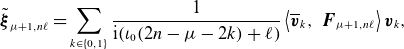 \begin{equation} \tilde {\boldsymbol{\xi }}_{\mu +1,n\ell } = \sum _{k\in \{0,1\}} \frac {1}{{\mathrm{i}}(\iota _0 (2n - \mu - 2k) + \ell )} \left \langle \overline {\boldsymbol{v}}_{k} , \ \boldsymbol{F}_{\mu +1,n\ell } \right \rangle \boldsymbol{v}_{k}, \end{equation}
where $\overline {\boldsymbol{v}}_k$
are the corresponding left eigenvectors due to
$\overline {\boldsymbol{v}}_k$
are the corresponding left eigenvectors due to $(\iota _0(2n-\mu -1)+\ell ){\mathrm{i}} I - \iota _0 J$
being skew-adjoint.
$(\iota _0(2n-\mu -1)+\ell ){\mathrm{i}} I - \iota _0 J$
being skew-adjoint.
There are two cases where the update (2.58) fails. The first case is when $2n - \mu - 2k = 0$
and
$2n - \mu - 2k = 0$
and $\ell = 0$
, occurring only when
$\ell = 0$
, occurring only when $\mu$
is even. This is the standard secularity that indicates that
$\mu$
is even. This is the standard secularity that indicates that $\iota _\mu$
must be updated, giving the condition that
$\iota _\mu$
must be updated, giving the condition that $\left \langle \overline {\boldsymbol{v}}_{0} , \ \boldsymbol{F}_{\mu +1,\mu /2,0} \right \rangle = \left \langle \overline {\boldsymbol{v}}_{1} , \ \boldsymbol{F}_{\mu +1,\mu /2+1,0} \right \rangle = 0$
for single-valued solutions, where we note that these formulae are equivalent for real magnetic fields. The resulting formula is
$\left \langle \overline {\boldsymbol{v}}_{0} , \ \boldsymbol{F}_{\mu +1,\mu /2,0} \right \rangle = \left \langle \overline {\boldsymbol{v}}_{1} , \ \boldsymbol{F}_{\mu +1,\mu /2+1,0} \right \rangle = 0$
for single-valued solutions, where we note that these formulae are equivalent for real magnetic fields. The resulting formula is
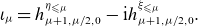 \begin{equation} \iota _\mu = h^{\eta _{\leqslant \mu }}_{\mu +1,\mu /2,0} - {\mathrm{i}} h^{\xi _{\leqslant \mu }}_{\mu +1,\mu /2,0}. \end{equation}
The second case of failure is when $\iota _0$
is rational, as then there are other values of
$\iota _0$
is rational, as then there are other values of $(\mu ,n,k,\ell )$
such that (2.58) is singular. This is attributed to the expanding number of
$(\mu ,n,k,\ell )$
such that (2.58) is singular. This is attributed to the expanding number of $\theta$
modes at each order, where higher-order poloidal perturbations resonate with the axis. To avoid this, extra resonant terms in the higher-order magnetic field must be introduced to avoid secularity (Duignan & Meiss Reference Duignan and Meiss2021) (equivalently, this requires adding terms to the Hamiltonian normal form). Here, we assume that
$\theta$
modes at each order, where higher-order poloidal perturbations resonate with the axis. To avoid this, extra resonant terms in the higher-order magnetic field must be introduced to avoid secularity (Duignan & Meiss Reference Duignan and Meiss2021) (equivalently, this requires adding terms to the Hamiltonian normal form). Here, we assume that $\iota _0$
is irrational so that the iteration is well defined.
$\iota _0$
is irrational so that the iteration is well defined.
We note that there is still one undetermined part of the problem: what value to choose for $\langle {\overline {\boldsymbol{v}}_{0}},{\tilde {\boldsymbol{\xi }}_{\mu +1,\mu /2,0}}\rangle$
and its complex conjugate. Because this is arbitrary, we currently set this coefficient to
$\langle {\overline {\boldsymbol{v}}_{0}},{\tilde {\boldsymbol{\xi }}_{\mu +1,\mu /2,0}}\rangle$
and its complex conjugate. Because this is arbitrary, we currently set this coefficient to $0$
. However, other options could be to choose this value to improve the radius of convergence or to match the flux (2.43). In summary, the straight field-line coordinate process is
$0$
. However, other options could be to choose this value to improve the radius of convergence or to match the flux (2.43). In summary, the straight field-line coordinate process is
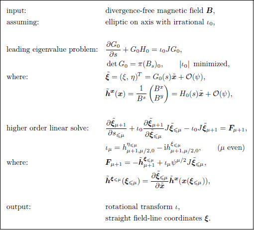
3. Ill-posedness and regularisation
In this section, we describe how the near-axis problem is ill-posed (§ 3.1) and how we can regularise the problem (§ 3.2). In § 3.3, we state how the near-axis expansion of $\phi$
converges under suitable input assumptions (Theorem (3.8) and Corollary (3.9)). Most proofs can be found in Appendix A, where the individual sections are referred to after each statement.
$\phi$
converges under suitable input assumptions (Theorem (3.8) and Corollary (3.9)). Most proofs can be found in Appendix A, where the individual sections are referred to after each statement.
3.1. Ill-posedness
We define a problem as ill-posed if it is not well-posed, where the standard definition of a well-posed problem is that:
-
(i) the solution exists;
-
(ii) the solution is unique;
-
(iii) the solution is continuous in the initial data.
We note that the interpretations of these statements depend on what space we require the solution to belong to and over which topology continuity is described in. For instance, it is straightforward to show existence and uniqueness in the sense of a formal power series.
Proposition 3.1.
Consider the near-axis problem in box (
2.30
), with all inputs in $C^{\infty }$
. Then, there exists a unique formal power series solution
$C^{\infty }$
. Then, there exists a unique formal power series solution $\phi _n(s)$
at each order.
$\phi _n(s)$
at each order.
Proof.
Simply notice that the residual at each order is $C^\infty$
if every previous order is. Then, because the inverse of
$C^\infty$
if every previous order is. Then, because the inverse of $\Delta _\perp$
of
$\Delta _\perp$
of $C^{\infty }$
functions is
$C^{\infty }$
functions is $C^\infty$
, we satisfy the Fredholm alternative, and we specify the null space the operator at each order, we have a unique solution.
$C^\infty$
, we satisfy the Fredholm alternative, and we specify the null space the operator at each order, we have a unique solution.
Note that this proposition says nothing about the convergence of the power series to a solution off-axis; it only shows that we can find the coefficients of the power series. So, formal existence does not necessarily imply good or consistent computational results.
Another straightforward existence result for harmonic inputs is the following.
Proposition 3.2.
Let $\boldsymbol{B} = \nabla \phi + \tilde {\boldsymbol{B}}$
be a valid vacuum magnetic field on
$\boldsymbol{B} = \nabla \phi + \tilde {\boldsymbol{B}}$
be a valid vacuum magnetic field on $\Omega _\sigma$
with a real-analytic axis
$\Omega _\sigma$
with a real-analytic axis $\boldsymbol{r}_0$
and
$\boldsymbol{r}_0$
and $\sigma \gt 0$
. Then, the near-axis expansion using the coefficients corresponding to
$\sigma \gt 0$
. Then, the near-axis expansion using the coefficients corresponding to $\phi$
converges uniformly on a smaller domain
$\phi$
converges uniformly on a smaller domain $\Omega _{\sigma '}$
with
$\Omega _{\sigma '}$
with $0\lt \sigma '\lt \sigma$
.
$0\lt \sigma '\lt \sigma$
.
Proof. See § A.1
Proposition (3.2) is a useful result because it says that vacuum fields can, in principle, be written as solutions to the infinite near-axis problem. However, this is a difficult theorem to use in practice, as it is difficult to verify a priori whether the input data to the near-axis expansion agree with a solution of Poisson’s equation.
So, for a more computational approach, we must define normed spaces of inputs and outputs that agree with notions of convergence. To intuit what the correct space may be, we observe that the radial direction behaves as a ‘time-like’ variable, whereas the $\theta$
and
$\theta$
and $s$
behave more like spatial variables. That is, the near-axis PDE can be thought of as propagating surface information off the axis. This motivates a decision to separate our treatment of these coordinates. Moreover, we desire convergence in a power series in the radial variable, so we choose to treat it in an analytic manner. In contrast, the coefficients
$s$
behave more like spatial variables. That is, the near-axis PDE can be thought of as propagating surface information off the axis. This motivates a decision to separate our treatment of these coordinates. Moreover, we desire convergence in a power series in the radial variable, so we choose to treat it in an analytic manner. In contrast, the coefficients $\phi _m(\theta ,s)$
are obtained by solving a linear PDE at each order, so we treat them in a Sobolev sense as a function of
$\phi _m(\theta ,s)$
are obtained by solving a linear PDE at each order, so we treat them in a Sobolev sense as a function of $\theta$
and
$\theta$
and $s$
.
$s$
.
To this end, let $\alpha = (\alpha _1,\alpha _2)$
be a multi-index of degree
$\alpha = (\alpha _1,\alpha _2)$
be a multi-index of degree $2$
and
$2$
and $\left | \alpha \right | = \sum _j \alpha _j$
. We define the
$\left | \alpha \right | = \sum _j \alpha _j$
. We define the $H^q$
Sobolev norm of functions
$H^q$
Sobolev norm of functions $f : \mathbb{T}^2 \to \mathbb{R}$
as
$f : \mathbb{T}^2 \to \mathbb{R}$
as
 \begin{equation} \left \lVert f \right \rVert ^2_{H^q} = \sum _{\left | \alpha \right | \leqslant q} \left \lVert D_\alpha f \right \rVert ^2_{L^2}, \end{equation}
where
 \begin{equation} D_\alpha f = \frac {\partial ^{\left | \alpha \right |}f}{\partial \theta ^{\alpha _1} \partial s^{\alpha _2}}, \qquad \left \lVert f \right \rVert ^2_{L^2} = \int _{\mathbb{T}^2}\left | f \right |^2 \hspace {1pt} \mathrm{d} \mu , \end{equation}
and $\mu$
is the Lebesgue measure on
$\mu$
is the Lebesgue measure on $\mathbb{T}^2$
. We additionally define the
$\mathbb{T}^2$
. We additionally define the $C^q$
norm of a
$C^q$
norm of a $q$
-times differentiable function
$q$
-times differentiable function $f : \mathbb{T}^2 \to \mathbb{R}$
as
$f : \mathbb{T}^2 \to \mathbb{R}$
as
 \begin{equation} \left \lVert f \right \rVert _{C^q} = \sum _{\left | \alpha \right |\leqslant q} \sup _{(\theta ,s)\in \mathbb{T}^2} \left | D_\alpha f(\theta ,s) \right |. \end{equation}
Then, we define the following convenient near-axis function space.
Definition 3.3.
Let $\sigma \gt 0$
and
$\sigma \gt 0$
and $W$
be a Banach space on functions on
$W$
be a Banach space on functions on $\mathbb{T}^2$
. We define a function
$\mathbb{T}^2$
. We define a function $f : \Omega _\sigma ^0 \to \mathbb{R}^d$
as
$f : \Omega _\sigma ^0 \to \mathbb{R}^d$
as $(\sigma ,W)$
-analytic if
$(\sigma ,W)$
-analytic if $f$
has a convergent near-axis expansion of the form
$f$
has a convergent near-axis expansion of the form
 \begin{equation} f(\rho ,\theta ,s) = \sum _{m=0}^\infty f_m(\theta , s)\rho ^m, \qquad f_m(\theta ,s) = \sum _{n=0}^m f_{mn}(s) e^{(2n-m){\mathrm{i}} \theta }, \end{equation}
where the norm
 \begin{equation} \left \lVert f \right \rVert _{\sigma ,W} = \sup _n \left (\sigma ^n \left \lVert f_n \right \rVert _{W}\right ) \end{equation}
is bounded. Here, convergence of the near-axis expansion is pointwise in $\rho$
and in norm in
$\rho$
and in norm in $(\theta ,s)$
, i.e. for all
$(\theta ,s)$
, i.e. for all $\rho \lt \sigma$
,
$\rho \lt \sigma$
,
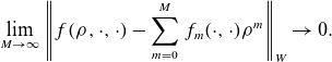 \begin{equation} \lim _{M\to \infty }\left \lVert f(\rho ,\cdot ,\cdot ) - \sum _{m=0}^M f_m(\cdot ,\cdot ) \rho ^m \right \rVert _{W} \to 0. \end{equation}
Paralleling standard linear regularity theory (Evans Reference Evans2010), we will consider near-axis solutions $\phi$
to belong to a Sobolev
$\phi$
to belong to a Sobolev $(\sigma ,H^q)$
-analytic space, while near-axis PDE coefficients belong to differentiable
$(\sigma ,H^q)$
-analytic space, while near-axis PDE coefficients belong to differentiable $(\sigma ,C^q)$
-analytic spaces. Because the coefficients of Poisson’s equation (2.21) are functions of the metric, control on the
$(\sigma ,C^q)$
-analytic spaces. Because the coefficients of Poisson’s equation (2.21) are functions of the metric, control on the $(\sigma ,C^q)$
-analytic norm of the coefficients in the Frenet–Serret coordinate system will be entirely determined by the differentiability class of the axis
$(\sigma ,C^q)$
-analytic norm of the coefficients in the Frenet–Serret coordinate system will be entirely determined by the differentiability class of the axis $\boldsymbol r_0 \in C^q(\mathbb{T})$
.
$\boldsymbol r_0 \in C^q(\mathbb{T})$
.
To build some intuition for $(\sigma ,W)$
-analytic functions, we turn to some straightforward facts about their convergence. Let
$(\sigma ,W)$
-analytic functions, we turn to some straightforward facts about their convergence. Let $f$
be
$f$
be $(\sigma ,W)$
-analytic. Then, for any
$(\sigma ,W)$
-analytic. Then, for any $F\geqslant \left \lVert f \right \rVert _{\sigma ,W}$
, the definition of the norm
$F\geqslant \left \lVert f \right \rVert _{\sigma ,W}$
, the definition of the norm $\left \lVert \cdot \right \rVert _{\sigma ,W}$
tells us that the coefficients are bounded as
$\left \lVert \cdot \right \rVert _{\sigma ,W}$
tells us that the coefficients are bounded as
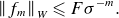 \begin{equation} \left \lVert f_m \right \rVert _{W} \leqslant F \sigma ^{-m}. \end{equation}
This means that surfaces of $f$
converge geometrically for
$f$
converge geometrically for $\rho ^* \lt \sigma$
in
$\rho ^* \lt \sigma$
in $W$
, i.e.
$W$
, i.e.
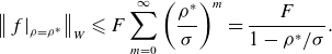 \begin{equation} \left \lVert \left . f \right |_{\rho =\rho ^*} \right \rVert _{W} \leqslant F\sum _{m=0}^{\infty } \left (\frac {\rho ^*}{\sigma }\right )^{m} = \frac {F}{1-\rho ^*/\sigma }. \end{equation}
For a more practical statement of pointwise convergence, we have the following proposition.
Proposition 3.4.
Let $f$
be
$f$
be $(\sigma ,C^q)$
-analytic for
$(\sigma ,C^q)$
-analytic for $q \geqslant 0$
. Then,
$q \geqslant 0$
. Then, $f$
is continuous and
$f$
is continuous and $q$
-times continuously differentiable in
$q$
-times continuously differentiable in $\Omega _\sigma ^0$
.
$\Omega _\sigma ^0$
.
Proof. See § A.2
Corollary 3.5.
Let $f$
be
$f$
be $(\sigma ,H^q)$
-analytic for
$(\sigma ,H^q)$
-analytic for $q \geqslant 2$
. Then,
$q \geqslant 2$
. Then, $f$
is
$f$
is $(\sigma ,C^{q-2})$
-analytic, continuous and
$(\sigma ,C^{q-2})$
-analytic, continuous and $(q-2)$
-times continuously differentiable in
$(q-2)$
-times continuously differentiable in $\Omega _\sigma ^0$
.
$\Omega _\sigma ^0$
.
Proof.
Because $H^q(\mathbb{T}^2)$
is continuously embedded in
$H^q(\mathbb{T}^2)$
is continuously embedded in $C^{q-2}(\mathbb{T}^2)$
,
$C^{q-2}(\mathbb{T}^2)$
, $f$
is also
$f$
is also $(\sigma ,C^{q-2})$
-analytic. Apply Proposition (3.4).
$(\sigma ,C^{q-2})$
-analytic. Apply Proposition (3.4).
A direct consequence of the preceding statements is that both $(\sigma ,C^0)$
-analytic and
$(\sigma ,C^0)$
-analytic and $(\sigma ,H^2)$
-analytic functions are continuous in 3-D, but
$(\sigma ,H^2)$
-analytic functions are continuous in 3-D, but $(\sigma ,H^1)$
-analytic functions need not be.
$(\sigma ,H^1)$
-analytic functions need not be.
Now, let us return to the question of ill-posedness. To define the norm of the input, let
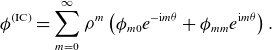 \begin{equation} \phi ^{(\text{IC})} = \sum _{m=0}^\infty \rho ^m \left (\phi _{m0} e^{-{\mathrm{i}} m \theta } + \phi _{mm} e^{{\mathrm{i}} m \theta } \right ). \end{equation}
This allows us to naturally define the norm of the input functions $\phi _{m0}$
and
$\phi _{m0}$
and $\phi _{mm}$
via a single
$\phi _{mm}$
via a single $(\sigma ,{H^q})$
-analytic norm. Using this, we prove that the problem is ill-posed in the following sense.
$(\sigma ,{H^q})$
-analytic norm. Using this, we prove that the problem is ill-posed in the following sense.
Theorem 3.6.
Let $\boldsymbol{r}_0, B_0, \phi _{m0}, \phi _{mm} \in C^{\infty }$
for
$\boldsymbol{r}_0, B_0, \phi _{m0}, \phi _{mm} \in C^{\infty }$
for $2 \leqslant m \lt \infty$
with
$2 \leqslant m \lt \infty$
with $\ell ',\kappa \gt 0$
and
$\ell ',\kappa \gt 0$
and $q_0 \geqslant 0$
. The near-axis solution
$q_0 \geqslant 0$
. The near-axis solution $\phi$
of (
2.30
) is not continuous to perturbations
$\phi$
of (
2.30
) is not continuous to perturbations $\delta \boldsymbol{r}_0, \delta B_0, \delta \phi _{m0}, \delta \phi _{mm} \in C^{\infty }$
under the
$\delta \boldsymbol{r}_0, \delta B_0, \delta \phi _{m0}, \delta \phi _{mm} \in C^{\infty }$
under the $C^{4+q_0}(\mathbb{T})$
norm on
$C^{4+q_0}(\mathbb{T})$
norm on $\boldsymbol{r}_0$
, the
$\boldsymbol{r}_0$
, the $H^{1+q_0}(\mathbb{T})$
norm on
$H^{1+q_0}(\mathbb{T})$
norm on $B_0$
, the
$B_0$
, the $(\sigma _0,H^{2+q_0})$
-analytic norm on
$(\sigma _0,H^{2+q_0})$
-analytic norm on $\phi ^{(\text{IC})}$
with
$\phi ^{(\text{IC})}$
with $\sigma _0\gt 0$
, and any
$\sigma _0\gt 0$
, and any $(\sigma ,H^q)$
-analytic norm on the output
$(\sigma ,H^q)$
-analytic norm on the output $\phi$
with
$\phi$
with $\sigma \gt 0$
and
$\sigma \gt 0$
and $q\geqslant 2$
, i.e. the near-axis expansion is ill-posed.
$q\geqslant 2$
, i.e. the near-axis expansion is ill-posed.
Proof. See § A.3
In other words, Theorem (3.6) tells us that smooth bounded perturbations in the input lead to unbounded deviations in the solution, even if the problem is initially prepared to be convergent. The characteristic form of the unbounded perturbations are high frequency in $s$
, which grow exponentially off-axis according to their wavenumber. When the near-axis expansion is discretised, this appears to be a poor condition number for the truncated problem. This motivates us to introduce a term in the near-axis expansion that damps the behaviour of the high-frequency modes.
$s$
, which grow exponentially off-axis according to their wavenumber. When the near-axis expansion is discretised, this appears to be a poor condition number for the truncated problem. This motivates us to introduce a term in the near-axis expansion that damps the behaviour of the high-frequency modes.
Before we continue, we note there is a strong connection between the ill-posedness of the near-axis expansion and the ill-posedness of coil design. It is typically the case that magnetic fields with large gradients are difficult to approximate using plasma coils far from the boundary (Kappel et al. Reference Kappel, Landreman and Malhotra2024). This is because high frequencies in coil design decay quickly towards the surface of the plasma – the opposite view of the problem of high frequencies growing outward from the axis. The effect is that it is difficult to match high frequencies on the plasma boundary, and coil design codes also require some form of regularisation (Landreman Reference Landreman2017).
3.2. Regularisation
We have just seen in Theorem (3.6) that the near-axis expansion described in box (2.30) is ill-posed. Ill-posedness can potentially cause significant problems for numerical simulations, with the primary one being that discretisation refinement – both in toroidal resolution and in the order of expansion – will not lead to convergence to a solution. Instead, the deviation from the correct answer typically increases with refinement.
In the proof of Theorem (3.6) (§ A.3), the problematic perturbations to the input have small amplitude and high poloidal wavenumber, leading to exponential growth off the axis with a rate proportional to the wavenumber. Here, we would like to damp the problematic high-wavenumber modes while maintaining the fidelity of the low-wavenumber modes. We do so by adding a high-order differential operator in the toroidal and poloidal directions, as high-order derivatives affect high wavenumbers significantly more than low wavenumbers. Specifically, we propose the following version of Poisson’s equation (2.21) with regularisation:
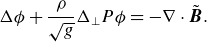 \begin{equation} \Delta \phi + \frac {\rho }{\sqrt {g}}\Delta _{\perp }P \phi = - \nabla \cdot \tilde {\boldsymbol{B}}. \end{equation}
The new term contains the regularising differential operator $\Delta _\perp P$
that is at least fourth order. The operator is composed of a product of the perpendicular Laplacian defined by
$\Delta _\perp P$
that is at least fourth order. The operator is composed of a product of the perpendicular Laplacian defined by
 \begin{equation} \Delta _{\perp } \phi = \frac {1}{\rho } \frac {\partial }{\partial \rho }\left ( \rho \frac {\partial \phi }{\partial \rho }\right ) + \frac {1}{\rho ^2} \frac {\partial ^2\phi }{\partial \theta ^2}, \end{equation}
and the regularising differential operator $P$
satisfying the following hypotheses.
$P$
satisfying the following hypotheses.
Hypotheses 3.7.
Let $q\geqslant 0$
and
$q\geqslant 0$
and $D \geqslant 1$
. We require
$D \geqslant 1$
. We require $P$
be an order
$P$
be an order $2D$
differential operator that satisfies the following:
$2D$
differential operator that satisfies the following:
-
(i) $P$
takes the form
(3.12)where
\begin{equation} P = \sum _{m=0}^{2D}\sum _{n=0}^{m} P^{(mn)}(s) \frac {\partial ^{m+n}}{\partial s^m \partial \theta ^n}, \end{equation}
$P^{(mn)}(s)\in C^{q}$
;
$P$
takes the form
(3.12)where
\begin{equation} P = \sum _{m=0}^{2D}\sum _{n=0}^{m} P^{(mn)}(s) \frac {\partial ^{m+n}}{\partial s^m \partial \theta ^n}, \end{equation}
$P^{(mn)}(s)\in C^{q}$
;
-
(ii)
$P$
is strongly elliptic, i.e. for some
$C\gt 0$
and for all
$(x,y)\in \mathbb{R}^2 \backslash \{0\}$
,(3.13)
\begin{equation} \sum _{n=0}^{2D} P^{(2D,n)}(s) x^{2D-n} y^n \geqslant C (x^2 + y^2)^D, \end{equation}
-
(iii)
$P$
is self-adjoint and semi positive-definite, i.e. for non-zero
$f,g \in H^{2D}(\mathbb{T}^2)$
,(3.14)
\begin{equation} \left \langle f , \ Pg \right \rangle = \left \langle Pf , \ g \right \rangle , \qquad \left \langle f , \ Pf \right \rangle \geqslant 0, \qquad \left \langle f , \ g \right \rangle := \int _{\mathbb{T}^2}f(\theta ,s) g(\theta ,s) \hspace {1pt} \mathrm{d} \theta \mathrm{d} s \end{equation}


We note that in hypothesis (i), the coefficients of $P$
do not depend on
$P$
do not depend on $\theta$
. This means poloidal Fourier modes ‘block diagonalise’
$\theta$
. This means poloidal Fourier modes ‘block diagonalise’ $P$
, i.e. for
$P$
, i.e. for $f(s) \in H^{q + 2D}$
, we have
$f(s) \in H^{q + 2D}$
, we have $P(f(s) e^{{\mathrm{i}} m \theta }) = g(s) e^{{\mathrm{i}} m \theta }$
for some
$P(f(s) e^{{\mathrm{i}} m \theta }) = g(s) e^{{\mathrm{i}} m \theta }$
for some $g(s) \in H^{q}$
. This is sufficient for
$g(s) \in H^{q}$
. This is sufficient for $P$
to map
$P$
to map $(\sigma ,H^{q+2D})$
-analytic functions to
$(\sigma ,H^{q+2D})$
-analytic functions to $(\sigma ,H^{q})$
-analytic functions, while
$(\sigma ,H^{q})$
-analytic functions, while $\theta$
dependence would make the operator non-analytic. It also means that
$\theta$
dependence would make the operator non-analytic. It also means that $P$
commutes with
$P$
commutes with $\Delta _{\perp }$
, i.e.
$\Delta _{\perp }$
, i.e. $P\Delta _\perp = \Delta _\perp P$
on sufficiently regular functions. Moreover, the hypotheses (ii) and (iii) are sufficient for
$P\Delta _\perp = \Delta _\perp P$
on sufficiently regular functions. Moreover, the hypotheses (ii) and (iii) are sufficient for $1+P$
to be invertible, which is necessary at each step of the iteration.
$1+P$
to be invertible, which is necessary at each step of the iteration.
In practice, we use the operator
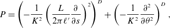 \begin{equation} P = \left (-\frac {1}{K^2}\left (\frac {L}{2\pi \ell '} \frac {\partial }{\partial s}\right )^2\right )^{D} + \left (- \frac {1}{K^2} \frac {\partial ^2}{\partial \theta ^2} \right )^{D}, \end{equation}
where $K \gt 0$
is the characteristic wavenumber of regularisation,
$K \gt 0$
is the characteristic wavenumber of regularisation, $2D\geqslant 2$
is the algebraic order of the frequency damping and
$2D\geqslant 2$
is the algebraic order of the frequency damping and $L = \oint \ell ' \hspace {1pt} \mathrm{d} s$
is the length of the magnetic axis. We have chosen the specific form of
$L = \oint \ell ' \hspace {1pt} \mathrm{d} s$
is the length of the magnetic axis. We have chosen the specific form of $P$
so that it is easy to implement numerically when the curve is in arclength coordinates (and therefore
$P$
so that it is easy to implement numerically when the curve is in arclength coordinates (and therefore $\ell '$
is constant, satisfying the smoothness requirement). Indeed, any polynomial in the arclength derivative
$\ell '$
is constant, satisfying the smoothness requirement). Indeed, any polynomial in the arclength derivative $(\ell ')^{-1}({\partial }/{\partial s})$
and the poloidal derivative
$(\ell ')^{-1}({\partial }/{\partial s})$
and the poloidal derivative $ ({\partial }/{\partial \theta })$
is simply inverted in Fourier space. Additionally, the parameter
$ ({\partial }/{\partial \theta })$
is simply inverted in Fourier space. Additionally, the parameter $K$
can be tuned from large (weak damping) to small (strong damping) to adjust the regularisation strength.
$K$
can be tuned from large (weak damping) to small (strong damping) to adjust the regularisation strength.
With regularisation, the new iterative form of the near-axis expansion (3.10) is
 \begin{equation} \left (m^2 + \frac {\partial ^2}{\partial \theta ^2}\right )(1 + P) \phi _m = -(\nabla \cdot \tilde {\boldsymbol{B}} + \Delta \phi _{\lt m})_{m-2}, \end{equation}
where we discuss the relevant regularity in Corollary (3.9). If we use the regularisation (3.15) and $s$
to be a scaled arclength coordinate so that
$s$
to be a scaled arclength coordinate so that $\ell ' = L/2\pi$
is constant, the componentwise version of the iteration is
$\ell ' = L/2\pi$
is constant, the componentwise version of the iteration is
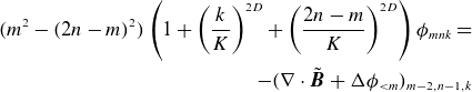 \begin{align} (m^2 - (2n-m)^2)\left (1 + \left (\frac { k}{K}\right )^{2D} + \left (\frac {2n-m}{K}\right )^{2D}\right )\phi _{mnk} = \nonumber \\ -(\nabla \cdot \tilde {\boldsymbol{B}} + \Delta \phi _{\lt m})_{m-2,n-1,k} \end{align}
for $0\lt n\lt m$
. We see that in the near-axis iteration, the regularisation damps the high-order modes by dividing by high-order polynomials in the poloidal and toroidal wavenumbers.
$0\lt n\lt m$
. We see that in the near-axis iteration, the regularisation damps the high-order modes by dividing by high-order polynomials in the poloidal and toroidal wavenumbers.
By construction, the regularisation has another benefit: the full problem can be represented as the divergence of a perturbed magnetic field $\boldsymbol{B}_K$
. If we let
$\boldsymbol{B}_K$
. If we let $G = Diag(1, \rho ^{-2}, 0)$
, we have
$G = Diag(1, \rho ^{-2}, 0)$
, we have
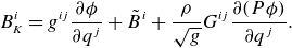 \begin{equation} B_K^i = g^{ij} \frac {\partial \phi }{\partial q^j} + \tilde {B}^i + \frac {\rho }{\sqrt {g}} G^{ij} \frac {\partial (P \phi )}{\partial q^j} . \end{equation}
The fact that there is still an underlying divergence-free field is important for the relation between the near-axis expansion and Hamiltonian mechanics. Therefore, the regularised near-axis expansion of the field $\boldsymbol{B}_K$
can be expressed by the problem
$\boldsymbol{B}_K$
can be expressed by the problem
 \begin{equation} \nabla \times \boldsymbol{B}_K = \boldsymbol J_K, \qquad \nabla \cdot \boldsymbol{B}_K = 0, \end{equation}
where $\boldsymbol J_K$
is a fictitious regularising current. In contrast, the regularisation means
$\boldsymbol J_K$
is a fictitious regularising current. In contrast, the regularisation means $\boldsymbol{B} = \nabla \phi + \tilde {\boldsymbol{B}}$
is not divergence-free. To find the flux surfaces, we note that the procedure in box (2.60) in no way depends on the magnetic field being curl-free. As such, we perform the same steps for finding flux coordinates for
$\boldsymbol{B} = \nabla \phi + \tilde {\boldsymbol{B}}$
is not divergence-free. To find the flux surfaces, we note that the procedure in box (2.60) in no way depends on the magnetic field being curl-free. As such, we perform the same steps for finding flux coordinates for $\boldsymbol{B}_K$
as with
$\boldsymbol{B}_K$
as with $\boldsymbol{B}$
.
$\boldsymbol{B}$
.
3.3. Convergence of the regularised expansion
Consider a PDE of the form
 \begin{equation} \Delta _\perp (1+P)\phi = f + L^{(a)}\phi , \end{equation}
where $P$
satisfies Hypotheses (3.7),
$P$
satisfies Hypotheses (3.7), $f$
is
$f$
is $(\sigma _0,H^{q})$
-analytic for
$(\sigma _0,H^{q})$
-analytic for $q\geqslant 0$
and
$q\geqslant 0$
and $\sigma _0\gt 0$
, and
$\sigma _0\gt 0$
, and
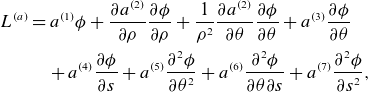 \begin{align} L^{(a)} &= a^{(1)}\phi + \frac {\partial a^{(2)}}{\partial \rho } \frac {\partial \phi }{\partial \rho } + \frac {1}{\rho ^2} \frac {\partial a^{(2)}}{\partial \theta }\frac {\partial \phi }{\partial \theta } + a^{(3)} \frac {\partial \phi }{\partial \theta } \nonumber \\ &\quad+ a^{(4)} \frac {\partial \phi }{\partial s} + a^{(5)} \frac {\partial ^2\phi }{\partial \theta ^2} + a^{(6)} \frac {\partial ^2\phi }{\partial \theta \partial s} + a^{(7)} \frac {\partial ^2 \phi }{\partial s^2}, \end{align}
and each $a^{(j)}$
is a
$a^{(j)}$
is a $(\Sigma , C^{q})$
-analytic for
$(\Sigma , C^{q})$
-analytic for $\Sigma \gt \sigma _0$
. By a straightforward application of chain rule, we see that (3.10) satisfies this form for
$\Sigma \gt \sigma _0$
. By a straightforward application of chain rule, we see that (3.10) satisfies this form for $\boldsymbol r_0 \in H^{4+q}$
and
$\boldsymbol r_0 \in H^{4+q}$
and $B_0 \in H^{1+q}$
, where
$B_0 \in H^{1+q}$
, where $\Sigma \leqslant \min \kappa ^{-1}$
(see proof of Corollary 3.9 in Appendix A.5). Equation (3.20) also encompasses other coordinate and regularisation assumptions of the near-axis expansion, including those not defined by Frenet–Serret coordinates.
$\Sigma \leqslant \min \kappa ^{-1}$
(see proof of Corollary 3.9 in Appendix A.5). Equation (3.20) also encompasses other coordinate and regularisation assumptions of the near-axis expansion, including those not defined by Frenet–Serret coordinates.
The implicit near-axis iteration for (3.20) can be written as
 \begin{equation} (\Delta _\perp (1+ P) \phi )_m = \left [f + L^{(a)}\right ]_{m}\!. \end{equation}
The form of the iteration automatically respects the Fredholm condition, so it is solvable at each order (see the proof of Theorem (3.8)). So, to solve at each order of the iteration, we can invert to find that
 \begin{equation} \phi _m = \phi ^{(\text{IC})}_m + \left( (1+P)^{-1} \Delta _\perp ^{+} \left [f + L^{(a)}\phi \right ]\right )_{m}\!, \end{equation}
where $\phi ^{(\text{IC})}$
is
$\phi ^{(\text{IC})}$
is $(\sigma _0,H^{q+2})$
-analytic of the form (3.9) and we define the pseudoinverse
$(\sigma _0,H^{q+2})$
-analytic of the form (3.9) and we define the pseudoinverse $\Delta ^+_\perp$
as
$\Delta ^+_\perp$
as
 \begin{equation} \Delta _\perp ^{+} (\rho ^m e^{{\mathrm{i}} (2n-m) \theta }) = \frac {1}{(m+2)^2 - (2n-m)^2} \rho ^{m+2} e^{{\mathrm{i}} (2n-m) \theta } \qquad \text{ for }0\leqslant n \leqslant m. \end{equation}
Given this iteration, we find the following theorem for its convergence.
Theorem 3.8.
Let $0\lt \sigma _0\lt \Sigma$
,
$0\lt \sigma _0\lt \Sigma$
, $q \geqslant 1$
and
$q \geqslant 1$
and $D\geqslant 1$
. Then, let
$D\geqslant 1$
. Then, let $f$
be
$f$
be $(\sigma _0,H^q)$
-analytic,
$(\sigma _0,H^q)$
-analytic, $a^{(j)}$
for
$a^{(j)}$
for $1\leqslant j \leqslant 7$
be
$1\leqslant j \leqslant 7$
be $(\Sigma , C^q)$
-analytic,
$(\Sigma , C^q)$
-analytic, $\phi ^{(\text{IC})}$
as defined by (3.9) be
$\phi ^{(\text{IC})}$
as defined by (3.9) be $(\sigma _0,H^{q+2D})$
-analytic and
$(\sigma _0,H^{q+2D})$
-analytic and $P$
satisfy Hypotheses (3.7). Then, there is a unique
$P$
satisfy Hypotheses (3.7). Then, there is a unique $(\sigma ,H^{q+2D})$
-analytic near-axis solution
$(\sigma ,H^{q+2D})$
-analytic near-axis solution $\phi$
of (3.20) with initial data
$\phi$
of (3.20) with initial data $\phi ^{(\text{IC})}$
. Moreover, this solution operator is continuous in
$\phi ^{(\text{IC})}$
. Moreover, this solution operator is continuous in $a^{(j)}$
and satisfies the bound
$a^{(j)}$
and satisfies the bound
 \begin{equation} \left \lVert \phi \right \rVert _{\sigma ,H^{q+2D}} \leqslant C \left \lVert f \right \rVert _{\sigma _0,H^q} + C \left \lVert \phi ^{(\text{IC})} \right \rVert _{\sigma _0,H^{q+2D}}\!. \end{equation}
Proof. See Appendix A.4.
This theorem can be translated to the Frenet–Serret problem.
Corollary 3.9.
Let $\sigma \gt 0$
,
$\sigma \gt 0$
, $q \geqslant 1$
and
$q \geqslant 1$
and $D\geqslant 1$
. Then, let
$D\geqslant 1$
. Then, let $\boldsymbol r_0 \in C^{4+q}$
in scaled arclength coordinates with
$\boldsymbol r_0 \in C^{4+q}$
in scaled arclength coordinates with $\ell ' = L/2\pi \gt 0$
and
$\ell ' = L/2\pi \gt 0$
and $\kappa \gt 0$
,
$\kappa \gt 0$
, $B_0 \in H^{1+q}$
,
$B_0 \in H^{1+q}$
, $\phi ^{(\text{IC})}$
be
$\phi ^{(\text{IC})}$
be $(\sigma _0,H^{q+2D})$
-analytic, and
$(\sigma _0,H^{q+2D})$
-analytic, and $P$
be defined as in (
3.15
). Then, for some
$P$
be defined as in (
3.15
). Then, for some $\sigma \gt 0$
satisfying
$\sigma \gt 0$
satisfying $\sigma \leqslant \sigma _0$
and
$\sigma \leqslant \sigma _0$
and $\sigma \lt \min \kappa ^{-1}$
, the near-axis solution
$\sigma \lt \min \kappa ^{-1}$
, the near-axis solution $\phi$
of (
3.10
) is
$\phi$
of (
3.10
) is $(\sigma ,H^{q+2D})$
-analytic, continuous in
$(\sigma ,H^{q+2D})$
-analytic, continuous in $\boldsymbol r_0$
and satisfies
$\boldsymbol r_0$
and satisfies
 \begin{equation} \left\lVert{\phi}\right\rVert_{\sigma,H^{q+2D}} \leq C \left\lVert{B_0}\right\rVert_{H^{1+q}} + C \left\lVert{{\phi^{(\text{IC})}}}\right\rVert_{\sigma_0,H^{q+2D}}. \end{equation}
Furthermore, the associated divergence-free field $\boldsymbol{B}_K$
is well-defined and is
$\boldsymbol{B}_K$
is well-defined and is $(\sigma ',H^q)$
-analytic for all
$(\sigma ',H^q)$
-analytic for all $\sigma '\lt \sigma$
.
$\sigma '\lt \sigma$
.
Proof. See Appendix A.5.
There are two primary reasons why Theorem (3.8) is useful for computation. First, it gives a guarantee that the norm of the inputs controls the size of the output. For instance, in the context of stellarator optimisation, if an appropriate Sobolev penalty is put on $\boldsymbol r_0$
,
$\boldsymbol r_0$
, $B_0$
and
$B_0$
and $\phi ^{(\text{IC})}$
, then one can expect the output to be appropriately bounded. Second, because the output is
$\phi ^{(\text{IC})}$
, then one can expect the output to be appropriately bounded. Second, because the output is $(\sigma ,H^{q+2D})$
-analytic, it tells us that truncations of the near-axis expansion are approximations of the true solution. So, we can be more confident that finite asymptotic series are approximately correct, at least for the regularised problem.
$(\sigma ,H^{q+2D})$
-analytic, it tells us that truncations of the near-axis expansion are approximations of the true solution. So, we can be more confident that finite asymptotic series are approximately correct, at least for the regularised problem.
It is worth noting that while Theorem (3.8) tells us there is a solution to the regularised problem, it does not tell us that the solution solves the original problem. To address this, we can develop an a posteriori handle on the error.
Proposition 3.10.
Consider the hypotheses of Theorem (
3.8
) with $q\geqslant 2$
. Additionally, suppose
$q\geqslant 2$
. Additionally, suppose $0\lt \sigma '\lt \sigma$
,
$0\lt \sigma '\lt \sigma$
, $L=\Delta _\perp - L^{(a)}$
is a second-order negative-definite operator on
$L=\Delta _\perp - L^{(a)}$
is a second-order negative-definite operator on $H^{2}_{0}(\Omega _{\sigma '}^0)$
, and
$H^{2}_{0}(\Omega _{\sigma '}^0)$
, and $\phi ^{\sigma '} = \phi (\sigma ',\theta ,s)$
. Then, the solution
$\phi ^{\sigma '} = \phi (\sigma ',\theta ,s)$
. Then, the solution $\phi$
of the near-axis expansion is the unique solution in
$\phi$
of the near-axis expansion is the unique solution in $H^{q+2D}(\Omega _{\sigma '}^0)$
of the boundary value problem
$H^{q+2D}(\Omega _{\sigma '}^0)$
of the boundary value problem
 \begin{equation} P \Delta _\perp \phi + L \phi = f, \qquad \left . \phi \right |_{\rho = \sigma '} = \phi ^{\sigma '}\!. \end{equation}
Moreover, let $\tilde \phi$
be the solution to
$\tilde \phi$
be the solution to
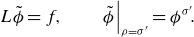 \begin{equation} L \tilde \phi = f, \qquad \left . \tilde \phi \right |_{\rho =\sigma '} = \phi ^{\sigma '}\!. \end{equation}
Then,
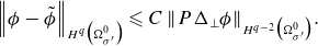 \begin{equation} \left \lVert \phi - \tilde \phi \right \rVert _{H^{q}\big(\Omega _{\sigma '}^0\big)} \leqslant C \left \lVert P \Delta _\perp \phi \right \rVert _{H^{q-2}\big(\Omega _{\sigma '}^0\big)}\!. \end{equation}
Proof. See Appendix A.6.
In other words, this tells us that given a solution to the regularised problem, we can bound the distance to a non-regularised boundary value problem via the norm of $P \Delta _\perp \phi$
. This applies directly to the Frenet–Serret case because the Laplacian is negative-definite. So, given a solution, this gives us an estimate of the error. As before, we can summarise the new problem (cf. box (2.30)):
$P \Delta _\perp \phi$
. This applies directly to the Frenet–Serret case because the Laplacian is negative-definite. So, given a solution, this gives us an estimate of the error. As before, we can summarise the new problem (cf. box (2.30)):
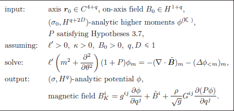
4. Numerical method
To numerically solve the regularised near-axis expansion algorithm in (3.30), we use a pseudospectral method. Pseudospectral methods use spectral representations of the solution for derivatives, while scalar multiplication and other operations occur on a set of collocation points. The spectral form of the series is
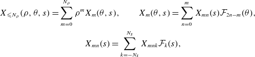 \begin{align} X_{\leqslant N_\rho }(\rho ,\theta ,s) = \sum _{m=0}^{N_\rho } \rho ^m & X_m(\theta , s), \qquad X_m(\theta , s) = \sum _{n=0}^m X_{mn}(s) \mathcal{F}_{2n-m}(\theta ) , \nonumber \\ & X_{mn}(s) = \sum _{k = -N_s}^{N_s} X_{mnk} \mathcal{F}_k(s), \end{align}
where $N_\rho$
and
$N_\rho$
and $N_s$
are integers specifying the resolution of the series and
$N_s$
are integers specifying the resolution of the series and
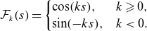 \begin{equation} \mathcal{F}_k(s) = \begin{cases} \cos (k s), & k \geqslant 0, \\ \sin (-k s), & k \lt 0. \end{cases} \end{equation}
Derivatives of the series are numerically evaluated by
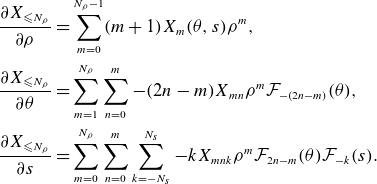 \begin{align} \frac {\partial X_{\leqslant N_\rho }}{\partial \rho } &= \sum _{m=0}^{N_\rho -1} (m+1) X_{m}(\theta , s) \rho ^{m}, \nonumber \\ \frac {\partial X_{\leqslant N_\rho }}{\partial \theta } &= \sum _{m=1}^{N_\rho } \sum _{n=0}^m -(2n-m) X_{mn} \rho ^{m} \mathcal{F}_{-(2n-m)}(\theta ),\nonumber \\ \frac {\partial X_{\leqslant N_\rho }}{\partial s} &= \sum _{m=0}^{N_\rho } \sum _{n=0}^m \sum _{k=-N_s}^{N_s} -k X_{mnk} \rho ^{m} \mathcal{F}_{2n-m}(\theta ) \mathcal{F}_{-k}(s). \end{align}
For algebraic operations such as series multiplication, composition and inversion, we discretise each $X_m$
on a grid
$X_m$
on a grid $X_m(\theta _{mj}, s_\ell )$
, where
$X_m(\theta _{mj}, s_\ell )$
, where
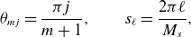 \begin{equation} \theta _{mj} = {\frac {\pi j}{m+1}}, \qquad s_\ell = \frac {2 \pi \ell }{M_s}, \end{equation}
where $0 \leqslant j \leqslant m$
,
$0 \leqslant j \leqslant m$
, $0 \leqslant \ell \lt M_s$
and
$0 \leqslant \ell \lt M_s$
and $M_s \geqslant 2N_s+1$
is the number of
$M_s \geqslant 2N_s+1$
is the number of $s$
-collocation points. Typically, we choose
$s$
-collocation points. Typically, we choose $M_s = 4N_s + 3$
to oversample in
$M_s = 4N_s + 3$
to oversample in $s$
by a factor of over
$s$
by a factor of over $2$
. This choice anti-aliases the numerical method by removing high harmonics generated in the collocation space (Boyd Reference Boyd2001). We note that the
$2$
. This choice anti-aliases the numerical method by removing high harmonics generated in the collocation space (Boyd Reference Boyd2001). We note that the $\theta$
-collocation points
$\theta$
-collocation points $\theta _{mj}$
are spaced around the half-circle instead of the full circle, owing to the fact that analytic coefficients satisfy the symmetry
$\theta _{mj}$
are spaced around the half-circle instead of the full circle, owing to the fact that analytic coefficients satisfy the symmetry
 \begin{equation} X_m(\theta +\pi ,s) = (-1)^m X_m(\theta ,s). \end{equation}
For even $m$
, (4.5) tells us that
$m$
, (4.5) tells us that $X_m$
is periodic in
$X_m$
is periodic in $2\theta$
and the resulting transformation is the discrete Fourier transform (DFT) in that angular coordinate. However,
$2\theta$
and the resulting transformation is the discrete Fourier transform (DFT) in that angular coordinate. However, $X_m$
is anti-periodic in
$X_m$
is anti-periodic in $\theta$
for odd
$\theta$
for odd $m$
and the collocation on the half-circle can interpreted as a symmetry reduction of the DFT on the full circle.
$m$
and the collocation on the half-circle can interpreted as a symmetry reduction of the DFT on the full circle.
To transform between Fourier and spatial representations at each order $m$
, let
$m$
, let $\mathsf{X}^{\mathrm{c}}_{m} = [X_m(\theta _{mj},s_{\ell })] \in \mathbb{R}^{(m+1) \times M_s}$
be the matrix of collocation values and
$\mathsf{X}^{\mathrm{c}}_{m} = [X_m(\theta _{mj},s_{\ell })] \in \mathbb{R}^{(m+1) \times M_s}$
be the matrix of collocation values and $\mathsf{X}^{s}_m = [X_{mnk}] \in \mathbb{R}^{(m+1)\times (2N_s+1)}$
be the matrix of Fourier coefficients. Then, we define the transition matrices
$\mathsf{X}^{s}_m = [X_{mnk}] \in \mathbb{R}^{(m+1)\times (2N_s+1)}$
be the matrix of Fourier coefficients. Then, we define the transition matrices $[(\mathsf{F}_{\theta }^{m,m'})_{jn}] = [\mathcal{F}_{2n-m}(\theta _{m'j})] \in \mathbb{R}^{(m+1)\times (m'+1)}$
and
$[(\mathsf{F}_{\theta }^{m,m'})_{jn}] = [\mathcal{F}_{2n-m}(\theta _{m'j})] \in \mathbb{R}^{(m+1)\times (m'+1)}$
and $[(\mathsf{F}_s)_{k\ell }]=[\mathcal{F}_{k}(s_\ell )] \in \mathbb{R}^{(2N_s+1)\times M_s}$
. The transformation from spectral coefficients to collocation nodes is expressed by
$[(\mathsf{F}_s)_{k\ell }]=[\mathcal{F}_{k}(s_\ell )] \in \mathbb{R}^{(2N_s+1)\times M_s}$
. The transformation from spectral coefficients to collocation nodes is expressed by
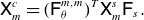 \begin{equation} \mathsf{X}^c_m = (\mathsf{F}_{\theta }^{m,m})^T \mathsf{X}^s_m \mathsf{F}_s. \end{equation}
Similarly, the inverse transform happens via
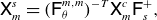 \begin{equation} \mathsf{X}^s_m = (\mathsf{F}_{\theta }^{m,m})^{-T} \mathsf{X}^c_m \mathsf{F}_s^+, \end{equation}
where the pseudo-inverse is $\mathsf{F}_s^+ = \mathsf{F}_s^T D_s^{-1}$
and
$\mathsf{F}_s^+ = \mathsf{F}_s^T D_s^{-1}$
and $D_s = \mathsf{F}_s \mathsf{F}_s^T \in \mathbb{R}^{(2N_s+1)\times (2N_s+1)}$
is diagonal with
$D_s = \mathsf{F}_s \mathsf{F}_s^T \in \mathbb{R}^{(2N_s+1)\times (2N_s+1)}$
is diagonal with $(D_s)_{jj}=(2N_s+1)$
for
$(D_s)_{jj}=(2N_s+1)$
for $j=0$
and
$j=0$
and $(D_s)_{jj} = (2N_s+1)/2$
for
$(D_s)_{jj} = (2N_s+1)/2$
for $-N_s\leqslant j\leqslant N_s$
,
$-N_s\leqslant j\leqslant N_s$
, $j\neq 0$
. This transformation is currently performed via full matrix–matrix multiplication, but it could be accelerated for large systems by the fast Fourier transform.
$j\neq 0$
. This transformation is currently performed via full matrix–matrix multiplication, but it could be accelerated for large systems by the fast Fourier transform.
The final basic operation we use is to raise the order of the $\theta$
-collocation. To see why this is necessary, consider the simple case of three monomial power series:
$\theta$
-collocation. To see why this is necessary, consider the simple case of three monomial power series: $X = \rho ^{m} X_m$
,
$X = \rho ^{m} X_m$
, $Y = \rho ^{m'} Y_{m'}$
and
$Y = \rho ^{m'} Y_{m'}$
and $Z = XY = \rho ^{m+m'} Z_{m+m'} = \rho ^{m+m'} X_m Y_{m'}$
. Then, the multiplication on the collocation nodes as
$Z = XY = \rho ^{m+m'} Z_{m+m'} = \rho ^{m+m'} X_m Y_{m'}$
. Then, the multiplication on the collocation nodes as
 \begin{equation} Z(\theta _{m+m',j}, s_\ell ) = \rho ^{m+m'} X(\theta _{m+m',j}, s_\ell ) Y(\theta _{m+m',j}, s_j). \end{equation}
So, to obtain the correct collocation on $Z_{m+m'}$
, we need to change the
$Z_{m+m'}$
, we need to change the $\theta$
-collocation on
$\theta$
-collocation on $X_{m}$
from
$X_{m}$
from $\theta _{mj}$
to
$\theta _{mj}$
to $\theta _{m+m',j}$
and similarly for
$\theta _{m+m',j}$
and similarly for $Y_{m'}$
. To do this, we use the
$Y_{m'}$
. To do this, we use the $\theta$
-collocation matrices to find
$\theta$
-collocation matrices to find
 \begin{equation} \mathsf{Z}^c_{m+m'} = \left [(F_{\theta }^{m,m+m'})^T(F_{\theta }^{m,m})^{-T} \mathsf{X}^c_m\right ] \odot \left [(F_{\theta }^{m',m+m'})^T(F_{\theta }^{m',m'})^{-T} \mathsf{Y}^c_m\right ], \end{equation}
where $\odot$
is the Hadamard (element-wise) product, and
$\odot$
is the Hadamard (element-wise) product, and $\mathsf{Y}^c_{m'}$
and
$\mathsf{Y}^c_{m'}$
and $\mathsf{Z}^c_{m+m'}$
are the collocation matrices of
$\mathsf{Z}^c_{m+m'}$
are the collocation matrices of $Y_{m'}$
and
$Y_{m'}$
and $Z_{m+m'}$
. With this operation, the operations outlined in Appendix B can be performed on the collocated nodes.
$Z_{m+m'}$
. With this operation, the operations outlined in Appendix B can be performed on the collocated nodes.
We note that choosing the correct amount of modes in $s$
presents the most difficult numerical problem in computing the near-axis expansion. As the order increases, high-order residuals are increasingly nonlinear in the lower orders, causing a broadening of the spectrum in
$s$
presents the most difficult numerical problem in computing the near-axis expansion. As the order increases, high-order residuals are increasingly nonlinear in the lower orders, causing a broadening of the spectrum in $s$
. If the inputs to the expansion do not have a sufficiently narrow bandwidth, this will result in broad higher-order residuals, particularly when finding flux coordinates. Both the regularisation and the anti-aliasing effects of choosing
$s$
. If the inputs to the expansion do not have a sufficiently narrow bandwidth, this will result in broad higher-order residuals, particularly when finding flux coordinates. Both the regularisation and the anti-aliasing effects of choosing $F_s$
to be rectangular help alleviate the issue of broad bandwidth, but in practice, we have found that it remains important to choose smooth inputs, especially for finding flux surfaces.
$F_s$
to be rectangular help alleviate the issue of broad bandwidth, but in practice, we have found that it remains important to choose smooth inputs, especially for finding flux surfaces.
5. Examples
We now investigate the numerical convergence of the near-axis expansion to high orders. Our focus is on characterising the convergence of the input (figure 4), the convergence of the output magnetic field (figure 5), the convergence of the magnetic surfaces (figures 7, 8) and the role of regularisation (figures 5, 6). Through our two examples – the rotating ellipse and the precise QA equilibrium of Landreman–Paul (Landreman & Paul Reference Landreman and Paul2022) – we find that the radius of convergence of every series is closely related to the distance from the magnetic axis to the coils $\sigma _{\mathrm{coil}}$
. This radius appears to limit the convergence of every other series of interest, including the magnetic surfaces that extend beyond this distance.
$\sigma _{\mathrm{coil}}$
. This radius appears to limit the convergence of every other series of interest, including the magnetic surfaces that extend beyond this distance.
All computations in this section were performed on a personal laptop. The code used to perform the expansions can be found at the StellaratorNearAxis.jl package (Ruth Reference Ruth2024a ).
5.1. Equilibrium initialisation
Coil sets for the rotating ellipse and Landreman–Paul examples. The colour indicates the normalised $\boldsymbol{B} \cdot \boldsymbol N$
error on the outer closed flux surface.
$\boldsymbol{B} \cdot \boldsymbol N$
error on the outer closed flux surface.
A major task in computing high-order near-axis expansions is choosing the input coefficients $\phi ^{(\text{IC})}$
in box (3.30). While low-order expansions can often be expressed in physically intuitive variables parametrising the rotation and stretching of elliptical magnetic surfaces, it is not as intuitive how to determine the high-order coefficients of
$\phi ^{(\text{IC})}$
in box (3.30). While low-order expansions can often be expressed in physically intuitive variables parametrising the rotation and stretching of elliptical magnetic surfaces, it is not as intuitive how to determine the high-order coefficients of $\phi ^{(\text{IC})}$
. In practice, the best option for finding equilibria would likely be via optimisation. However, for the purposes of demonstration, we initialise our inputs by a more direct method: via magnetic coils (see figure 3).
$\phi ^{(\text{IC})}$
. In practice, the best option for finding equilibria would likely be via optimisation. However, for the purposes of demonstration, we initialise our inputs by a more direct method: via magnetic coils (see figure 3).
The primary advantage of using coils for equilibrium initialisation is accuracy. The accuracy comes from the fact that the coil field can be expanded analytically about the axis, giving a direct input to the near-axis expansion. This circumvents the potentially error-prone problem of interpolating stellarator equilibria. Coils also provide an accurate ground truth to which to compare our equilibrium. In the following subsections, we use this to assess the accuracy of the near-axis expansion, both close to the axis and farther away.
The coil optimisation method employed here follows the approach described by Wechsung et al. (Reference Wechsung, Landreman, Giuliani, Cerfon and Stadler2022) and Jorge et al. (Reference Jorge, Giuliani and Loizu2024) using the code SIMSOPT (Landreman et al. Reference Landreman, Medasani, Wechsung, Giuliani, Jorge and Zhu2021). Coils are modelled as single closed 3-D filaments of current $\boldsymbol \Gamma ^{(i)} : \mathbb{T} \to \mathbb{R}^3$
. Each coil
$\boldsymbol \Gamma ^{(i)} : \mathbb{T} \to \mathbb{R}^3$
. Each coil $i$
is modelled as a periodic function in Cartesian coordinates where
$i$
is modelled as a periodic function in Cartesian coordinates where
 \begin{equation} \boldsymbol \Gamma ^{(j)}(s)=\boldsymbol c_{0}^{(j)}+\sum _{\ell =1}^{N_F}\left [\boldsymbol c_{\ell }^{(j)}\cos (\ell \theta )+\boldsymbol s_{\ell }^{(j)}\sin (\ell \theta )\right ], \end{equation}
where each $\boldsymbol c_{\ell }^{(j)}, \boldsymbol s_{\ell }^{(j)} \in \mathbb{R}^3$
, yielding a total of
$\boldsymbol c_{\ell }^{(j)}, \boldsymbol s_{\ell }^{(j)} \in \mathbb{R}^3$
, yielding a total of $3\times (2N_F +1)$
degrees of freedom per coil. In this work, we used
$3\times (2N_F +1)$
degrees of freedom per coil. In this work, we used $N_F=12$
, with four coils per half-field period for Landreman–Paul case and eight coils per half-field period for the ellipse. The degrees of freedom for the coil shapes are then
$N_F=12$
, with four coils per half-field period for Landreman–Paul case and eight coils per half-field period for the ellipse. The degrees of freedom for the coil shapes are then
 \begin{equation} \boldsymbol x_{\text{coils}}=[\boldsymbol c_{l}^{(j)},\boldsymbol s_{l}^{(j)}, I_j], \end{equation}
with $I_j$
the current that goes through each coil. We take advantage of stellarator and rotational symmetries to only optimise a set of
$I_j$
the current that goes through each coil. We take advantage of stellarator and rotational symmetries to only optimise a set of $N_c$
coils per half-field period. This leads to a total of
$N_c$
coils per half-field period. This leads to a total of $2 \times n_{\text{fp}} \times N_c$
modular coils, where
$2 \times n_{\text{fp}} \times N_c$
modular coils, where $n_{\text{fp}}$
is the number of toroidal field periods with
$n_{\text{fp}}$
is the number of toroidal field periods with $n_{\text{fp}} = 2$
for Landreman–Paul and
$n_{\text{fp}} = 2$
for Landreman–Paul and $n_{\text{fp}} = 5$
for the rotating ellipse. The remaining coils are determined by symmetry. The magnetic field
$n_{\text{fp}} = 5$
for the rotating ellipse. The remaining coils are determined by symmetry. The magnetic field $ \textbf{B}_{\text{ext}}$
of each coil is evaluated using the Biot–Savart law
$ \textbf{B}_{\text{ext}}$
of each coil is evaluated using the Biot–Savart law
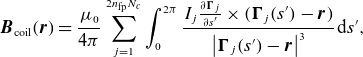 \begin{equation} \boldsymbol{B}_{\mathrm{coil}}(\boldsymbol{r}) = \frac {\mu _0}{4\pi } \sum _{j=1}^{2 n_{\mathrm{fp}} N_c} \int _{0}^{2\pi } \frac {I_j \frac {\partial \boldsymbol \Gamma _j}{\partial s'} \times (\boldsymbol \Gamma _j(s') - \boldsymbol{r})}{\left | \boldsymbol \Gamma _j(s') - \boldsymbol{r} \right |^3} \hspace {1pt} \mathrm{d} s', \end{equation}
where $s'$
parametrises the coil curve. Each coil is divided into 150 quadrature points, and the cost functions used to regularise the optimisation problem use the minimum distance between two coils, the length of each coil, their curvature and mean-squared curvature (see Wechsung et al. Reference Wechsung, Landreman, Giuliani, Cerfon and Stadler2022).
$s'$
parametrises the coil curve. Each coil is divided into 150 quadrature points, and the cost functions used to regularise the optimisation problem use the minimum distance between two coils, the length of each coil, their curvature and mean-squared curvature (see Wechsung et al. Reference Wechsung, Landreman, Giuliani, Cerfon and Stadler2022).
Using the coil magnetic field (5.3), we find the magnetic axis $\boldsymbol{r}_0$
via a shooting method. Then, using the near-axis coordinate representation of
$\boldsymbol{r}_0$
via a shooting method. Then, using the near-axis coordinate representation of $\boldsymbol{r}$
in (2.2), we expand the quadrature rule of (5.3) using the operations in Appendix B to find a near-axis expansion for the magnetic field
$\boldsymbol{r}$
in (2.2), we expand the quadrature rule of (5.3) using the operations in Appendix B to find a near-axis expansion for the magnetic field $\boldsymbol{B}(\rho ,\theta ,s)$
. Given the near-axis field, it is straightforward to compute
$\boldsymbol{B}(\rho ,\theta ,s)$
. Given the near-axis field, it is straightforward to compute $B_0$
by
$B_0$
by
 \begin{equation} B_0(s) = \boldsymbol{t}(s) \cdot \boldsymbol{B}(0,0,s), \end{equation}
and $\phi$
is found by a near-axis expansion of the path integral (note that
$\phi$
is found by a near-axis expansion of the path integral (note that $\phi =0$
on the axis)
$\phi =0$
on the axis)
 \begin{equation} \phi (\rho ,\theta ,s) = \int _{0}^\rho (\boldsymbol{B}(\rho ',\theta ,s) - \tilde {\boldsymbol{B}}(\rho ',\theta ,s)) \cdot (\cos (\theta ) \boldsymbol{n}(s) + \sin (\theta ) \boldsymbol{b}(s)) \hspace {1pt} \mathrm{d} \rho '. \end{equation}
Finally, the coefficients $\phi _{m0}$
and
$\phi _{m0}$
and $\phi _{mm}$
of this are used as input for
$\phi _{mm}$
of this are used as input for $\phi ^{(\text{IC})}$
. The input is computed to the
$\phi ^{(\text{IC})}$
. The input is computed to the $N_\rho =9$
orders in
$N_\rho =9$
orders in $\rho$
with
$\rho$
with $N_{s,\mathrm{RE}}=100$
and
$N_{s,\mathrm{RE}}=100$
and $N_{,s\mathrm{LP}}=50$
Fourier modes in
$N_{,s\mathrm{LP}}=50$
Fourier modes in $s$
for the rotating ellipse and Landreman–Paul, respectively (see (4.1)), where we use the subscript ‘RE’ for the rotating ellipse and ‘LP’ for Landreman–Paul wherever necessary.
$s$
for the rotating ellipse and Landreman–Paul, respectively (see (4.1)), where we use the subscript ‘RE’ for the rotating ellipse and ‘LP’ for Landreman–Paul wherever necessary.
To begin our analysis of the examples, we consider the inputs to the near-axis expansion. Corollary (3.9) suggests that there are two length scales dictated by the inputs. First is the radius of curvature of the axis. Letting $\Sigma = \min _s \kappa ^{-1}(s)$
be the radius of curvature, we find
$\Sigma = \min _s \kappa ^{-1}(s)$
be the radius of curvature, we find
 \begin{equation} \Sigma_\textrm{RE} = 0.987, \qquad \Sigma_\textrm{LP} = 0.681. \end{equation}
The other length scale of interest is the radius of convergence $\sigma _0$
of
$\sigma _0$
of $\phi ^{(\text{IC})}$
in the
$\phi ^{(\text{IC})}$
in the $(\sigma _0,H^{q+2D})$
-analytic norm. However, to the orders to which we compute, this radius appears to depend on the exponent
$(\sigma _0,H^{q+2D})$
-analytic norm. However, to the orders to which we compute, this radius appears to depend on the exponent $q+2D$
. To determine the most informative exponent, we consider the work by Kappel et al. (Reference Kappel, Landreman and Malhotra2024), where it was shown that the normalised gradient of the magnetic field is a strong predictor for plasma–coil separation. Because the
$q+2D$
. To determine the most informative exponent, we consider the work by Kappel et al. (Reference Kappel, Landreman and Malhotra2024), where it was shown that the normalised gradient of the magnetic field is a strong predictor for plasma–coil separation. Because the $H^2(\mathbb{T}^2)$
norm measures the size of the second derivative of
$H^2(\mathbb{T}^2)$
norm measures the size of the second derivative of $\phi ^{(\text{IC})}_m$
(and therefore the gradient of the input magnetic field), we conjecture this corresponds to the most practical exponent.
$\phi ^{(\text{IC})}_m$
(and therefore the gradient of the input magnetic field), we conjecture this corresponds to the most practical exponent.
To verify this, we first compute the minimum axis-to-coil distance $\sigma _{\mathrm{coil}}$
for both configurations to be
$\sigma _{\mathrm{coil}}$
for both configurations to be
 \begin{equation} \sigma _{\mathrm{coil,RE}}=0.241, \qquad \sigma _{\mathrm{coil,LP}} = 0.350. \end{equation}
We note that $\sigma _{\mathrm{coil}}\lt \Sigma$
for both configurations, indicating that the distance-to-coil is the limiting factor for convergence (cf. Corollary (3.9)). In figure 4, we plot the
$\sigma _{\mathrm{coil}}\lt \Sigma$
for both configurations, indicating that the distance-to-coil is the limiting factor for convergence (cf. Corollary (3.9)). In figure 4, we plot the $H^2$
norms of
$H^2$
norms of $\phi ^{(\text{IC})}_m$
versus
$\phi ^{(\text{IC})}_m$
versus $A \sigma _{\mathrm{coil}}^{-m}$
, where the coefficient
$A \sigma _{\mathrm{coil}}^{-m}$
, where the coefficient $A$
is found via a best fit for both configurations. In both cases, we find there is remarkable agreement, indicating that the
$A$
is found via a best fit for both configurations. In both cases, we find there is remarkable agreement, indicating that the $H^2$
radius of convergence of
$H^2$
radius of convergence of $\phi ^{(\text{IC})}$
could be used as a proxy for distance-to-coils.
$\phi ^{(\text{IC})}$
could be used as a proxy for distance-to-coils.
5.2. Magnetic field convergence
Plot of the coefficient norm $\lVert \phi ^{(\text{IC})}_m\rVert _{H^2}$
versus the order
$\lVert \phi ^{(\text{IC})}_m\rVert _{H^2}$
versus the order $m$
(markers) and best-fit lines
$m$
(markers) and best-fit lines $A \sigma _{\mathrm{coil}}^{-m}$
(lines), where
$A \sigma _{\mathrm{coil}}^{-m}$
(lines), where $\sigma _{\mathrm{coil}}$
is the axis-to-coil distance.
$\sigma _{\mathrm{coil}}$
is the axis-to-coil distance.
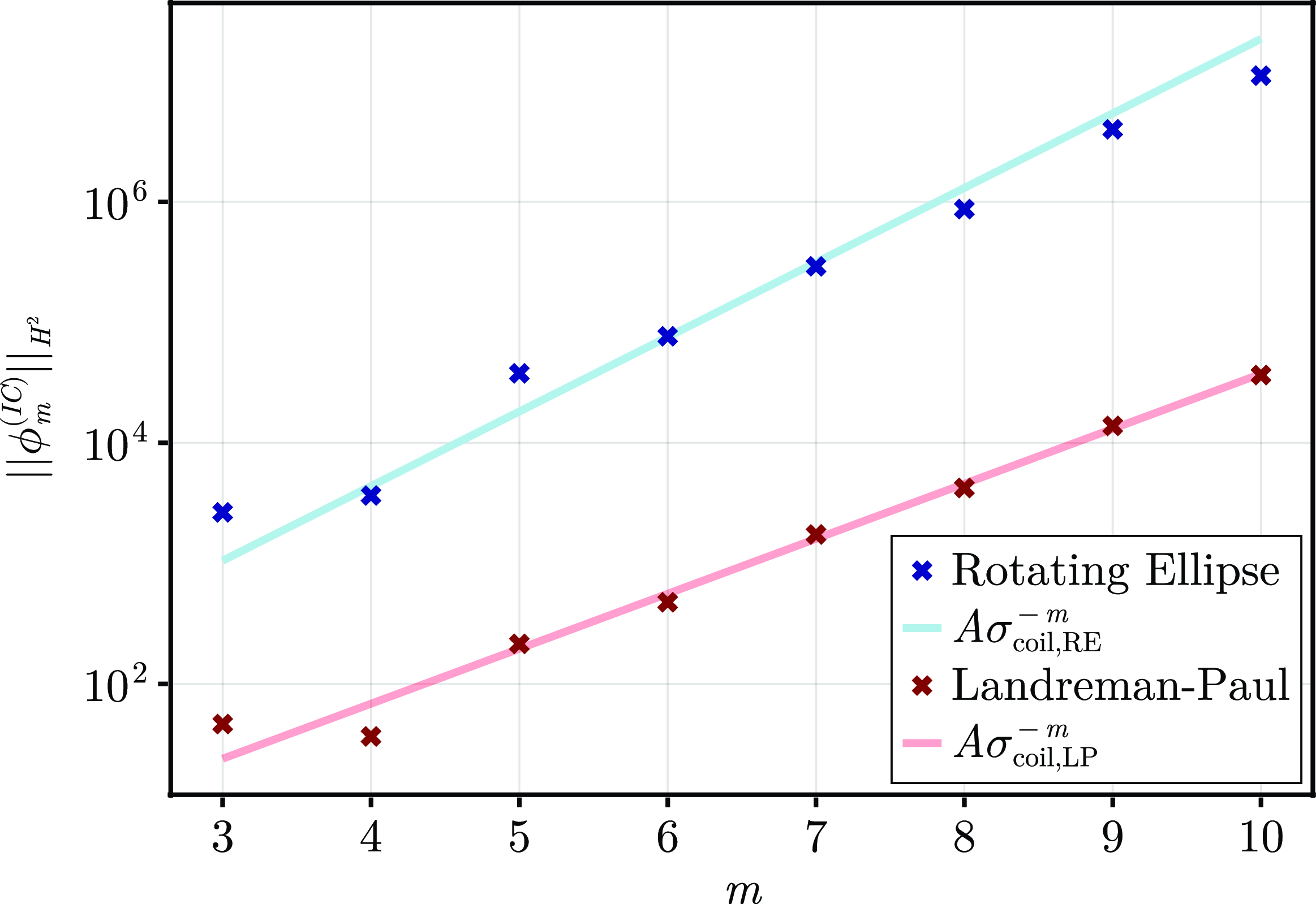
Next, we compute the near-axis expansion via the procedure in box (3.30). We perform the expansion both without regularisation ( $P=0$
) and with the regularisation operator in (3.15). For the regularised runs, we use
$P=0$
) and with the regularisation operator in (3.15). For the regularised runs, we use $D=2$
throughout and vary
$D=2$
throughout and vary $K$
between
$K$
between $10$
and
$10$
and $200$
to assess how the equilibrium changes between strong and weak regularisation, respectively.
$200$
to assess how the equilibrium changes between strong and weak regularisation, respectively.
As a first test of the output convergence, we compare the coil magnetic field against the unregularised expansion. Because the input is harmonic, we expect that the near-axis expansion will converge from Proposition (3.2) (unless floating-point errors overwhelm the solution, which is not observed to this order). We verify this by computing the $L^2$
magnetic field error on surfaces about the axis
$L^2$
magnetic field error on surfaces about the axis
 \begin{equation} \left \lVert \boldsymbol{B} - \boldsymbol{B}_{\mathrm{coil}} \right \rVert _{L^2(\partial \Omega _\sigma ^0)} = \frac {1}{4\pi ^2} \int _0^{2\pi } \int _{0}^{2\pi } \left | \boldsymbol{B}(\sigma ,\theta ,s) - \boldsymbol{B}_{\mathrm{coil}}(\sigma ,\theta ,s) \right |^2 \hspace {1pt} \mathrm{d} \theta \mathrm{d} s, \end{equation}
where $\boldsymbol{B}$
is computed from the near-axis expansion and
$\boldsymbol{B}$
is computed from the near-axis expansion and $\boldsymbol{B}_{\mathrm{coil}}$
is computed directly from Biot–Savart.
$\boldsymbol{B}_{\mathrm{coil}}$
is computed directly from Biot–Savart.
In figure 5(
a,b
), we plot the error (5.8) versus the normalised distance-from-axis $\sigma /\sigma _{\mathrm{coil}}$
. This error is computed for the approximation
$\sigma /\sigma _{\mathrm{coil}}$
. This error is computed for the approximation
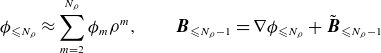 \begin{equation} \phi _{\leqslant N_\rho } \approx \sum _{m=2}^{N_\rho } \phi _m \rho ^m, \qquad \boldsymbol{B}_{\leqslant N_\rho -1} = \nabla \phi _{\leqslant N_\rho } + \tilde {\boldsymbol{B}}_{\leqslant N_\rho -1} \end{equation}
where $N_\rho$
is varied from
$N_\rho$
is varied from $1$
to
$1$
to $8$
. For both configurations, we find that the error of the magnetic field obeys the expected power law
$8$
. For both configurations, we find that the error of the magnetic field obeys the expected power law
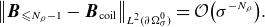 \begin{equation} \left \lVert \boldsymbol{B}_{\leqslant N_\rho -1} - \boldsymbol{B}_{\mathrm{coil}} \right \rVert _{L^2(\partial \Omega _\sigma ^0)} = \mathcal{O}\big(\sigma ^{-N_\rho }\big). \end{equation}
The error curves for varying $N_\rho$
meet at
$N_\rho$
meet at $\sigma = \sigma _{\mathrm{coil}}$
, indicating that the output radius of convergence is limited by the coils. This tells us that the limit of convergence
$\sigma = \sigma _{\mathrm{coil}}$
, indicating that the output radius of convergence is limited by the coils. This tells us that the limit of convergence $\sigma = \sigma _0$
is achievable in Corollary (3.9).
$\sigma = \sigma _0$
is achievable in Corollary (3.9).
(a,b) The error (5.8) as a function of the normalised distance from axis $\sigma /\sigma _{\mathrm{coil}}$
for varying orders of approximation
$\sigma /\sigma _{\mathrm{coil}}$
for varying orders of approximation $N_\rho$
. (c,d) The error (5.8) as a function of
$N_\rho$
. (c,d) The error (5.8) as a function of $\sigma /\sigma _{\mathrm{coil}}$
for varying values of the regularisation parameter
$\sigma /\sigma _{\mathrm{coil}}$
for varying values of the regularisation parameter $K$
(
$K$
( $K=\infty$
is unregularised).
$K=\infty$
is unregularised).
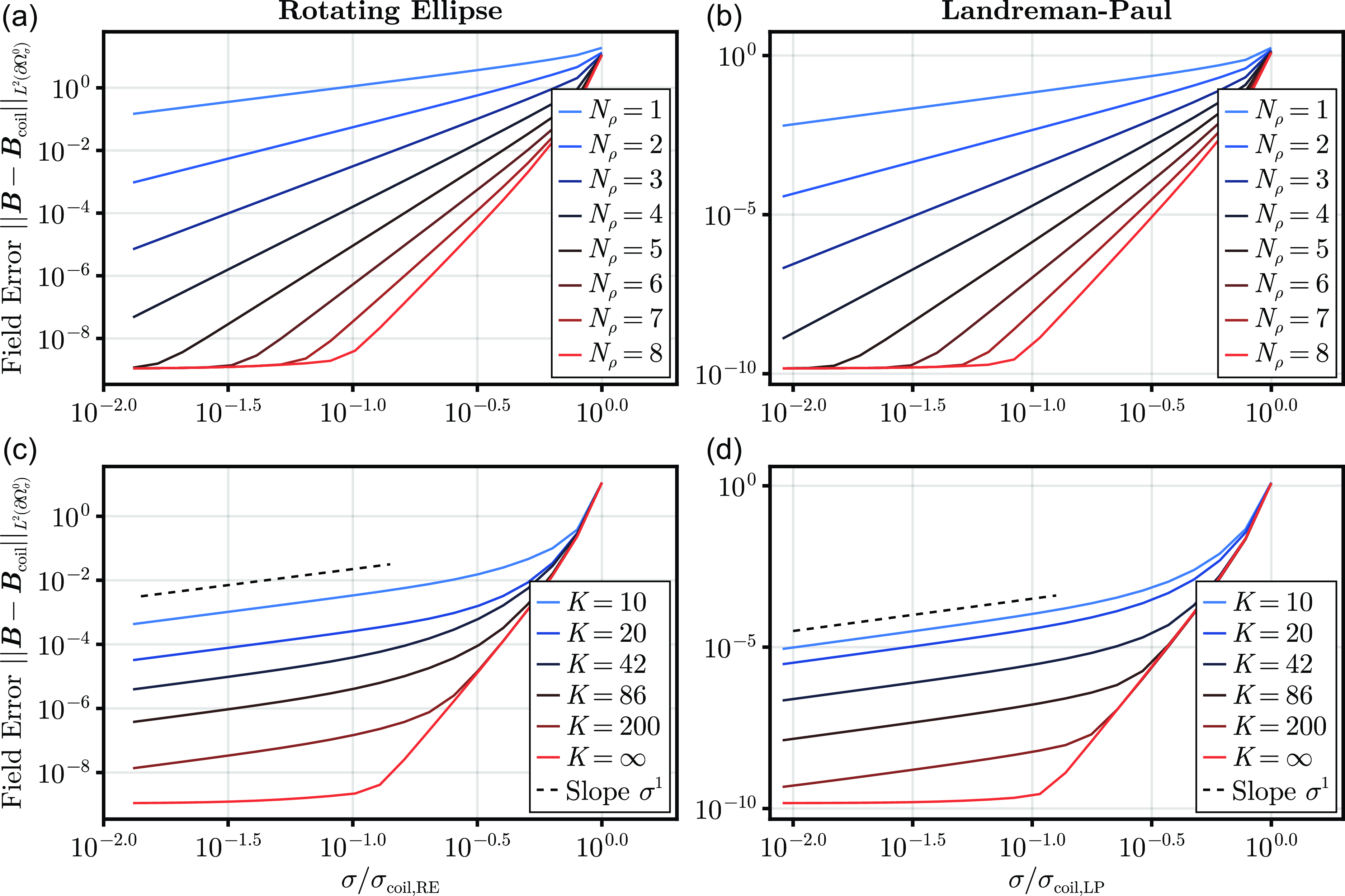
Turning to the effects of regularisation, we fix $N_\rho =9$
and plot the error (5.8) versus
$N_\rho =9$
and plot the error (5.8) versus $\sigma /\sigma _{\mathrm{coil}}$
for varying
$\sigma /\sigma _{\mathrm{coil}}$
for varying $K$
between
$K$
between $10$
and
$10$
and $200$
in figure 5(
c,d
). We also include the unregularised solution, labelled with
$200$
in figure 5(
c,d
). We also include the unregularised solution, labelled with $K=\infty$
. We find that as the regularisation becomes stronger (
$K=\infty$
. We find that as the regularisation becomes stronger ( $K$
decreases), the magnetic field loses fidelity near the core. We attribute to the increasing loss of accuracy of the high-wavenumber
$K$
decreases), the magnetic field loses fidelity near the core. We attribute to the increasing loss of accuracy of the high-wavenumber $s$
modes, while the low-wavenumber modes maintain accuracy. Then, far from the axis, the regularised error inflects to begin to agree with the rate of convergence of the unregularised solution. So, while the solution loses a high-wavenumber fidelity, the low wavenumbers maintain a similar level of accuracy. Comparing figures 5(
a,b
) with figure 5(
c,d
), we see that a regularised high-order expansion can achieve an equivalent error to an unregularised lower-order expansion near the axis while maintaining that fidelity far from the axis.
$s$
modes, while the low-wavenumber modes maintain accuracy. Then, far from the axis, the regularised error inflects to begin to agree with the rate of convergence of the unregularised solution. So, while the solution loses a high-wavenumber fidelity, the low wavenumbers maintain a similar level of accuracy. Comparing figures 5(
a,b
) with figure 5(
c,d
), we see that a regularised high-order expansion can achieve an equivalent error to an unregularised lower-order expansion near the axis while maintaining that fidelity far from the axis.
To address the role of regularisation more fully, however, we need to consider the fidelity of the expansion on less tuned inputs. To do this, we perturb $\boldsymbol{r}_0$
,
$\boldsymbol{r}_0$
, $B_0$
and
$B_0$
and $\phi ^{(\text{IC})}$
by the random functions as
$\phi ^{(\text{IC})}$
by the random functions as
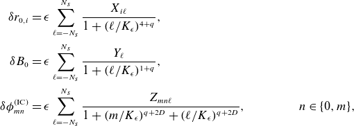 \begin{align} \delta r_{0,i} &= \epsilon \sum _{\ell = -N_s}^{N_s} \frac {X_{i\ell }}{1 + (\ell /K_{\epsilon })^{4+q}} , \nonumber \\ \delta B_0 &= \epsilon \sum _{\ell = -N_s}^{N_s}\frac {Y_{\ell }}{1 + (\ell /K_{\epsilon })^{1+q}} , \nonumber \\ \delta \phi ^{(\text{IC})}_{mn} &= \epsilon \sum _{\ell = -N_s}^{N_s} \frac {Z_{mn\ell }}{1 + (m/K_{\epsilon })^{q+2D} + (\ell /K_{\epsilon })^{q+2D}} , && \quad n\in \{0,m\}, \end{align}
where $X_{i\ell }$
,
$X_{i\ell }$
, $Y_\ell$
and
$Y_\ell$
and $Z_{mn\ell }$
are independent and identically distributed (i.i.d.) unit normal random variables,
$Z_{mn\ell }$
are independent and identically distributed (i.i.d.) unit normal random variables, $q = 2$
, and
$q = 2$
, and $\epsilon = 10^{-6}$
for the rotating ellipse and
$\epsilon = 10^{-6}$
for the rotating ellipse and $\epsilon =10^{-4}$
for Landreman–Paul. We have chosen the regularity of the perturbation to align with the inputs in box (3.30).
$\epsilon =10^{-4}$
for Landreman–Paul. We have chosen the regularity of the perturbation to align with the inputs in box (3.30).
Finite difference residual (5.12) as a function of the normalised distance from axis $\sigma /\sigma _{\mathrm{coil}}$
for the perturbed rotating ellipse and Landreman–Paul inputs (see (5.11)). For both plots, three lines are coloured and labelled, while the grey lines represent other values of
$\sigma /\sigma _{\mathrm{coil}}$
for the perturbed rotating ellipse and Landreman–Paul inputs (see (5.11)). For both plots, three lines are coloured and labelled, while the grey lines represent other values of $K$
interpolating between
$K$
interpolating between $K=10$
and
$K=10$
and $K=200$
.
$K=200$
.
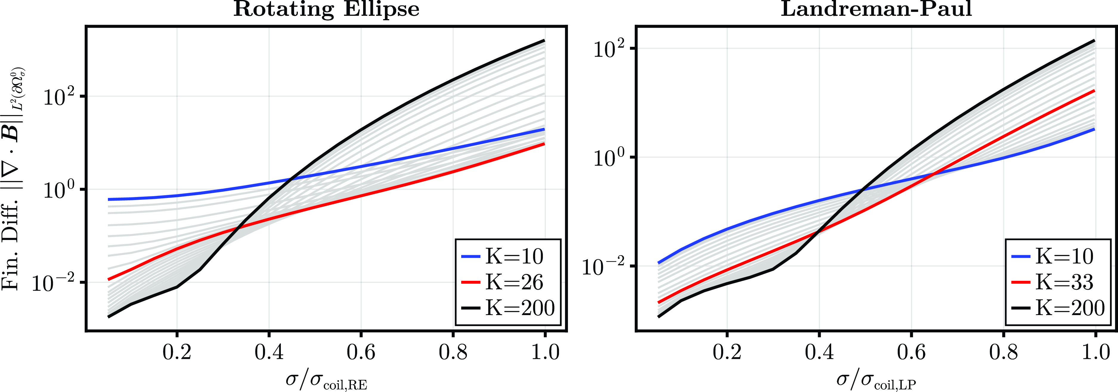
In figure 6, we consider the accuracy of the solution to the perturbed problem for $K$
varying between
$K$
varying between $10$
and
$10$
and $200$
for both examples with
$200$
for both examples with $N_\rho = 9$
fixed. To measure the accuracy, we no longer have a coil set with which to compare the solution directly. So, we instead measure the residual of Poisson’s equation
$N_\rho = 9$
fixed. To measure the accuracy, we no longer have a coil set with which to compare the solution directly. So, we instead measure the residual of Poisson’s equation
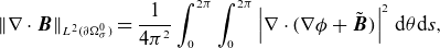 \begin{equation} \left \lVert \nabla \cdot \boldsymbol{B} \right \rVert _{L^2(\partial \Omega _\sigma ^0)} = \frac {1}{4\pi ^2} \int _0^{2\pi } \int _{0}^{2\pi } \left | \nabla \cdot (\nabla \phi + \tilde {\boldsymbol{B}}) \right |^2 \hspace {1pt} \mathrm{d} \theta \mathrm{d} s, \end{equation}
where we evaluate every derivative (including in the metric) via finite differences. For both perturbed examples, the best solution near the axis is the lightly regularised $K=200$
solution. However, beyond a certain radius between
$K=200$
solution. However, beyond a certain radius between $0.3\sigma _{\mathrm{coil}}$
and
$0.3\sigma _{\mathrm{coil}}$
and $0.4 \sigma _{\mathrm{coil}}$
, more regularised solutions improve upon the less regularised ones in the finite difference metric. For our examples, we find that
$0.4 \sigma _{\mathrm{coil}}$
, more regularised solutions improve upon the less regularised ones in the finite difference metric. For our examples, we find that $K=26$
for the rotating ellipse and
$K=26$
for the rotating ellipse and $K=33$
for Landreman–Paul are perhaps the best choices in practice. This figure potentially indicates a more general principle: the further from the axis one wants accuracy of the expansion, the more regularised the expansion likely has to be.
$K=33$
for Landreman–Paul are perhaps the best choices in practice. This figure potentially indicates a more general principle: the further from the axis one wants accuracy of the expansion, the more regularised the expansion likely has to be.
5.3. Magnetic coordinate convergence
Near-axis approximations of flux surfaces for varying orders of approximation $N_\rho$
(black); a Poincaré plot of the true coil magnetic field lines (colour). In the final
$N_\rho$
(black); a Poincaré plot of the true coil magnetic field lines (colour). In the final $N_\rho = 9$
panel, we plot a circle with radius
$N_\rho = 9$
panel, we plot a circle with radius $\sigma _{\mathrm{coil,LP}}$
in red.
$\sigma _{\mathrm{coil,LP}}$
in red.
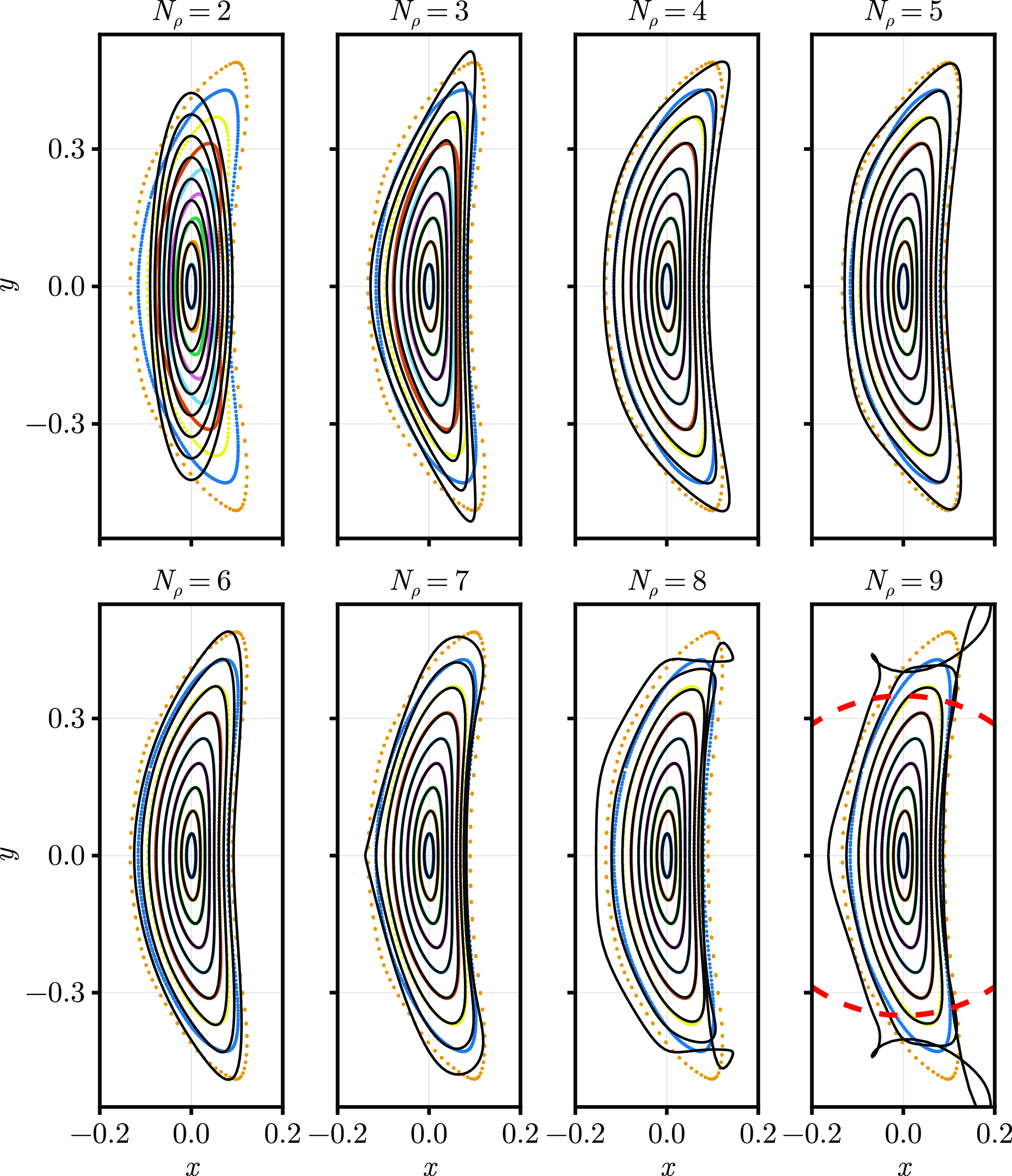
To compute straight field-line coordinates, we return to the unregularised Landreman–Paul configuration. Then, using the straight field-line magnetic coordinate equation from box (2.60), we compute the approximate coordinates $(\xi ,\eta )$
for
$(\xi ,\eta )$
for $N_\rho$
varying between
$N_\rho$
varying between $2$
and
$2$
and $9$
, where we note the
$9$
, where we note the $N_\rho =2$
approximation of
$N_\rho =2$
approximation of $\phi$
provides the leading-order field-line behaviour. To find flux surfaces, we then invert
$\phi$
provides the leading-order field-line behaviour. To find flux surfaces, we then invert $(\xi ,\eta )$
to find the distance-to-axis coordinates
$(\xi ,\eta )$
to find the distance-to-axis coordinates $(x(\xi ,\eta ,s),y(\xi ,\eta ,s))$
, where magnetic surfaces are parametrised by
$(x(\xi ,\eta ,s),y(\xi ,\eta ,s))$
, where magnetic surfaces are parametrised by $\xi ^2 + \eta ^2 = \psi$
.
$\xi ^2 + \eta ^2 = \psi$
.
In figure 7, we plot in black the computed surfaces on the $s=0$
Poincaré section for varying values of
$s=0$
Poincaré section for varying values of $N_\rho$
. For comparison, we plot the intersections of coil magnetic field lines in the background. At leading order, we see the surfaces are elliptical, while higher orders account for more shaping in the
$N_\rho$
. For comparison, we plot the intersections of coil magnetic field lines in the background. At leading order, we see the surfaces are elliptical, while higher orders account for more shaping in the $\theta$
direction. Then, as the order increases beyond
$\theta$
direction. Then, as the order increases beyond $5$
, the surfaces away from the core start diverging.
$5$
, the surfaces away from the core start diverging.
To investigate this divergence, we plot a red circle of constant radius $\sigma _{\mathrm{coil,LP}}$
in the
$\sigma _{\mathrm{coil,LP}}$
in the $N_\rho = 9$
panel. We see that the circle appears to separate the divergent surfaces from the convergent ones. We believe this is the likely reason for the divergence; however, there are still other possibilities.
$N_\rho = 9$
panel. We see that the circle appears to separate the divergent surfaces from the convergent ones. We believe this is the likely reason for the divergence; however, there are still other possibilities.


To assess the errors of surfaces closer to the axis, we turn to a more quantitative measure. To do this, we first use the method from Ruth & Bindel (Reference Ruth and Bindel2024) in the SymplecticMapTools.jl package (Ruth Reference Ruth2024b
) to compute invariant circles $(x_{\mathrm{coil}}(\theta ), y_{\mathrm{coil}}(\theta ))$
and the rotational transform
$(x_{\mathrm{coil}}(\theta ), y_{\mathrm{coil}}(\theta ))$
and the rotational transform $\iota _{\mathrm{coil}}$
on the cross-section from the Poincaré plot trajectories. Then, as a function of the inboard distance
$\iota _{\mathrm{coil}}$
on the cross-section from the Poincaré plot trajectories. Then, as a function of the inboard distance $x$
from the axis (see figure 7), we compute rotational transform and parametrisation errors as
$x$
from the axis (see figure 7), we compute rotational transform and parametrisation errors as
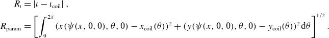 \begin{align} R_{\iota } &= \left | \iota - \iota _{\mathrm{coil}} \right |, \nonumber \\ R_{\mathrm{param}} &= \left [\int _{0}^{2\pi } (x(\psi (x,0,0),\theta ,0)-x_{\mathrm{coil}}(\theta ))^2 + (y(\psi (x,0,0),\theta ,0)-y_{\mathrm{coil}}(\theta ))^2 \hspace {1pt} \mathrm{d} \theta \right ]^{1/2}. \end{align}
In figure 8, we plot both errors with varying $N_\rho$
. In both cases, the rotational transform and parametrisation converge to high accuracy near the core. However, they begin to diverge before the the outermost surface, agreeing with the visual divergence in figure 7.
$N_\rho$
. In both cases, the rotational transform and parametrisation converge to high accuracy near the core. However, they begin to diverge before the the outermost surface, agreeing with the visual divergence in figure 7.
6. Conclusion
In this paper, we have investigated the convergence of the near-axis expansion in vacuum, both theoretically and numerically. From the theoretical point of view, we showed in Theorem (3.6) that the near-axis expansion is ill-posed, even in the relatively simple case of vacuum fields. However, as shown in Theorem (3.8), we found the near-axis problem can be regularised giving a guarantee of convergence for appropriately smooth input data. In particular, this tells us that a truncated near-axis expansion is an approximation to the solution of the regularised problem. Combining this with Proposition (3.10), we find can estimate the error of the regularised expansion from a true solution.
From the numerical results, we have verified that the near-axis expansion can converge in vacuum. This includes convergence of surfaces, where we have shown that the rotational transform and surface parametrisations can be approximated near the axis to high accuracy. Moreover, we demonstrated that the radius of convergence of the expansion is directly tied to the minimum distance to coils. Under perturbation, we found that the regularisation reduces the residual of Poisson’s equation far from the axis.
Our analysis suggests that the following four quantities should be kept in mind for future optimisation problems.
-
(i) The axis, on-axis field and higher moments should all be sufficiently regular for the expansion to converge (see box (3.30)). These can be enforced, e.g. by Sobolev norms on the inputs of the near-axis expansion.
-
(ii) In particular, the
$H^2$
-norm radius of convergence of
$\phi ^{(\text{IC})}$
appears to indicate the distance to coils from the axis (see figure 4). This gives a potential metric for plasma–coil distance. -
(iii) The axis curvature also limits to the radius of convergence, so this should be small relative to the desired minimum distance to coils.
-
(iv) In the case that the above terms are not sufficient, the error in Proposition (3.10) could be used to monitor the accuracy of the solutions.


Using these metrics, a moderate-order near-axis expansion (say, $4\leqslant N \leqslant 6$
) could be used to explore the space of stellarators more effectively. This could allow for the use of new near-axis optimisation problems.
$4\leqslant N \leqslant 6$
) could be used to explore the space of stellarators more effectively. This could allow for the use of new near-axis optimisation problems.
Looking forward, these results indicate that regularisation is likely also required for the near-axis expansion to converge in pressure. The form of (3.19) gives a potential path forward, where the regularisation could be expressed as a fictitious current. Physically, a link between regularisation and extended MHD models that provide additional current contributions can be studied. However, the issue of small denominators for near-rational $\iota _0$
(see (2.58)) will appear, which will combine with the regularised expansion in a non-trivial way in pressure. It remains to be seen whether regularisation can be used for improved convergence of these surfaces.
$\iota _0$
(see (2.58)) will appear, which will combine with the regularised expansion in a non-trivial way in pressure. It remains to be seen whether regularisation can be used for improved convergence of these surfaces.
Acknowledgments
The authors would like to acknowledge the helpful conversations with Tony Xu, Sean Yang, Gokul Nair and Joshua Burby in the development of this work.
Editor Per Helander thanks the referees for their advice in evaluating this article.
Funding
This work was supported by a grant from the Simons Foundation (No. 560651, D.B.) and by DOE DE-SC0024548. This material is based upon work supported by the National Science Foundation under Grant No.2409066. Any opinions, findings and conclusions or recommendations expressed in this material are those of the author(s) and do not necessarily reflect the views of the National Science Foundation.
Declaration of interests
The authors report no conflict of intererst.
Data availability statement
The data that support the finding of this study are openly available in the package StellaratorNearAxis.jl at the GitHub repository – https://github.com/ maxeruth/StellaratorNearAxis.jl .
Appendix A. Proofs
A.1 Proof of Proposition (3.2)
Because $\boldsymbol{B}$
is a vacuum field, its Cartesian components
$\boldsymbol{B}$
is a vacuum field, its Cartesian components $(B^1,B^2,B^3)$
are also harmonic and therefore real-analytic, meaning at each point on the axis
$(B^1,B^2,B^3)$
are also harmonic and therefore real-analytic, meaning at each point on the axis $\boldsymbol{r}_0(s)$
, it has a uniformly convergent Taylor series in a ball of size
$\boldsymbol{r}_0(s)$
, it has a uniformly convergent Taylor series in a ball of size $(\sqrt {2}-1)\sigma$
(Axler et al. Reference Axler, Bourdon and Ramey2001, Theorem 1.28). By choosing the coefficients
$(\sqrt {2}-1)\sigma$
(Axler et al. Reference Axler, Bourdon and Ramey2001, Theorem 1.28). By choosing the coefficients $\phi _{mn}$
to match the Taylor series at each point, we find that the near-axis expansion is uniformly convergent near the axis. Because
$\phi _{mn}$
to match the Taylor series at each point, we find that the near-axis expansion is uniformly convergent near the axis. Because $\boldsymbol{B}$
is harmonic, the coefficients must satisfy the near-axis problem (2.30). Finally, because the solution to the near-axis expansion is unique (3.1), the proposition is proven.
$\boldsymbol{B}$
is harmonic, the coefficients must satisfy the near-axis problem (2.30). Finally, because the solution to the near-axis expansion is unique (3.1), the proposition is proven.
A.2 Proof of Proposition (3.4)
We start with a lemma on derivatives on $(\sigma ,W)$
-analytic functions.
$(\sigma ,W)$
-analytic functions.
Lemma A.1.
Let $(x,y) = (\rho \cos \theta , \rho \sin \theta )$
and
$(x,y) = (\rho \cos \theta , \rho \sin \theta )$
and $W$
be
$W$
be $\mathcal{C}^q(\mathbb{T}^2)$
or
$\mathcal{C}^q(\mathbb{T}^2)$
or $H^q(\mathbb{T}^2)$
for
$H^q(\mathbb{T}^2)$
for $q\geqslant 0$
. The derivatives
$q\geqslant 0$
. The derivatives $({\partial }/{\partial x})$
and
$({\partial }/{\partial x})$
and $({\partial }/{\partial y})$
are bounded operators from
$({\partial }/{\partial y})$
are bounded operators from $(\sigma ,W)$
-analytic functions to
$(\sigma ,W)$
-analytic functions to $(\sigma ',W)$
-analytic functions for all
$(\sigma ',W)$
-analytic functions for all $0\lt \sigma '\lt \sigma$
.
$0\lt \sigma '\lt \sigma$
.
Proof.
We will prove this for the $x$
derivative, as the proof for the
$x$
derivative, as the proof for the $y$
derivative is identical. First, we observe that
$y$
derivative is identical. First, we observe that $x$
derivatives preserve the analytic structure (3.4). Let
$x$
derivatives preserve the analytic structure (3.4). Let $f$
be
$f$
be $(\sigma ,W)$
-analytic, where
$(\sigma ,W)$
-analytic, where $W$
is
$W$
is $H^q$
or
$H^q$
or $\mathcal{C}^q$
for
$\mathcal{C}^q$
for $q \geqslant 1$
. In polar coordinates, we have
$q \geqslant 1$
. In polar coordinates, we have
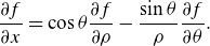 \begin{equation} \frac {\partial f}{\partial x} = \cos \theta \frac {\partial f}{\partial \rho }- \frac {\sin \theta }{\rho } \frac {\partial f}{\partial \theta }. \end{equation}
For both $\rho$
and
$\rho$
and $\theta$
, we have
$\theta$
, we have
 \begin{equation} \left \lVert \frac {\partial }{\partial \rho }\big(\rho ^m f_m\big) \right \rVert _{W} \leqslant m \rho ^{m-1} \left \lVert f_m \right \rVert _{W}, \qquad \left \lVert \frac {1}{\rho }\frac {\partial }{\partial \theta }\big(\rho ^m f_m\big) \right \rVert _{W} \leqslant m \rho ^{m-1} \left \lVert f_m \right \rVert _{W}. \end{equation}
Multiplying by $\sin \theta$
and
$\sin \theta$
and $\cos \theta$
is bounded on both
$\cos \theta$
is bounded on both $H^q$
and
$H^q$
and $\mathcal{C}^q$
, so
$\mathcal{C}^q$
, so
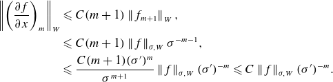 \begin{align} \left \lVert \left (\frac {\partial f}{\partial x}\right )_{m} \right \rVert _W &\leqslant C (m+1) \left \lVert f_{m+1} \right \rVert _W, \nonumber \\ &\leqslant C (m+1) \left \lVert f \right \rVert _{\sigma ,W} \sigma ^{-m-1}, \nonumber \\ &\leqslant \frac {C(m+1)(\sigma ')^m}{\sigma ^{m+1}} \left \lVert f \right \rVert _{\sigma ,W} (\sigma ')^{-m} \leqslant C \left \lVert f \right \rVert _{\sigma ,W} (\sigma ')^{-m}. \end{align}
Lemma A.2.
Let $q\geqslant 1$
. The derivatives
$q\geqslant 1$
. The derivatives $({\partial }/{\partial s})$
and
$({\partial }/{\partial s})$
and $({\partial }/{\partial \theta })$
are bounded operators from:
$({\partial }/{\partial \theta })$
are bounded operators from:
-
(i)
$(\sigma ,\mathcal{C}^q)$
-analytic functions to
$(\sigma ,\mathcal{C}^{q-1})$
-analytic functions; and
-
(ii)
$(\sigma ,H^q)$
-analytic functions to
$(\sigma ,H^{q-1})$
-analytic functions.


Proof.
Simply notice $({\partial }/{\partial s})$
and
$({\partial }/{\partial s})$
and $ ({\partial }/{\partial \theta })$
are bounded from
$ ({\partial }/{\partial \theta })$
are bounded from $\mathcal{C}^q$
to
$\mathcal{C}^q$
to $\mathcal{C}^{q-1}$
and from
$\mathcal{C}^{q-1}$
and from $H^{q}$
to
$H^{q}$
to $H^{q-1}$
.
$H^{q-1}$
.
Combining the two above lemmas, if we choose $\sigma '\lt \sigma$
,
$\sigma '\lt \sigma$
, $q \geqslant 0$
and
$q \geqslant 0$
and $f$
to be a
$f$
to be a $(\sigma ,\mathcal{C}^q)$
-analytic function, then for all
$(\sigma ,\mathcal{C}^q)$
-analytic function, then for all $m,n,\ell \gt 0$
such that
$m,n,\ell \gt 0$
such that $m+n+\ell \leqslant q$
, the function
$m+n+\ell \leqslant q$
, the function
 \begin{equation} g = \frac {\partial f}{\partial x^n \partial y^m \partial s^\ell } \end{equation}
is $(\sigma ', \mathcal{C}^0)$
-analytic. So, it suffices to prove that
$(\sigma ', \mathcal{C}^0)$
-analytic. So, it suffices to prove that $g$
is continuous in
$g$
is continuous in $\Omega _{\sigma '}^0$
.
$\Omega _{\sigma '}^0$
.
Let $0\lt \tilde {\rho } \lt \sigma '$
and
$0\lt \tilde {\rho } \lt \sigma '$
and $(\tilde {\theta },\tilde {s})\in \mathbb{T}^2$
. Then, choose
$(\tilde {\theta },\tilde {s})\in \mathbb{T}^2$
. Then, choose $\rho ^*$
such that
$\rho ^*$
such that $\tilde {\rho } \lt \rho ^*\lt \sigma '$
. We will show that
$\tilde {\rho } \lt \rho ^*\lt \sigma '$
. We will show that $g$
is continuous at the point
$g$
is continuous at the point $(\tilde {\rho },\tilde {\theta },\tilde {s})$
. Letting
$(\tilde {\rho },\tilde {\theta },\tilde {s})$
. Letting $\rho _1,\rho _2\leqslant \rho ^*$
, we can establish a Lipschitz bound of
$\rho _1,\rho _2\leqslant \rho ^*$
, we can establish a Lipschitz bound of $g$
in
$g$
in $\rho$
:
$\rho$
:
 \begin{align} \left | g(\rho _1, \theta , s) - g(\rho _2,\theta ,s) \right | &\leqslant \sum _{m=\beta }^\infty \left \lVert g_m \right \rVert _{C} \left | \rho _1^{m} - \rho _2^{m} \right | \nonumber \\ &\leqslant G\frac {\left | \rho _1-\rho _2 \right |}{\rho ^*} \sum _{m=1}^{\infty }m \left (\frac {\rho ^*}{\sigma }\right )^{m} \leqslant L \left | \rho _1-\rho _2 \right |. \end{align}
Now, let $(\rho _m,\theta _m,s_m) \to (\tilde {\rho },\tilde {\theta },\tilde {s})\in \Omega _\sigma ^0$
and
$(\rho _m,\theta _m,s_m) \to (\tilde {\rho },\tilde {\theta },\tilde {s})\in \Omega _\sigma ^0$
and $\sup (\rho _m) \lt \rho ^* \lt \sigma$
. We have
$\sup (\rho _m) \lt \rho ^* \lt \sigma$
. We have
 \begin{equation} \left | g(\rho _m,\theta _m,s_m) - g(\tilde {\rho },\tilde {\theta },\tilde {s}) \right | \leqslant L \left | \rho _m-\rho \right | + \left | g(\tilde {\rho },\theta _m,s_m)- g(\tilde {\rho },\tilde {\theta },\tilde {s}) \right |. \end{equation}
Because surfaces of $g$
converge in
$g$
converge in $C$
, both terms converge to zero giving our result.
$C$
, both terms converge to zero giving our result.
A.3 Proof of Theorem (3.6)
To prove this theorem, we will begin with a few facts about operators on $(\sigma ,q)$
-analytic functions.
$(\sigma ,q)$
-analytic functions.
Lemma A.3.
Let $f$
be
$f$
be $(\sigma ,H^q)$
-analytic and
$(\sigma ,H^q)$
-analytic and $g$
be
$g$
be $(\Sigma ,\mathcal{C}^q)$
-analytic where
$(\Sigma ,\mathcal{C}^q)$
-analytic where $0 \lt \sigma \leqslant \sigma _0 \lt \Sigma$
and
$0 \lt \sigma \leqslant \sigma _0 \lt \Sigma$
and $q\geqslant 0$
. Then,
$q\geqslant 0$
. Then, $fg$
is
$fg$
is $(\sigma ,H^q)$
-analytic with
$(\sigma ,H^q)$
-analytic with
 \begin{equation} \left \lVert fg \right \rVert _{\sigma ,q} \leqslant C \left \lVert g \right \rVert _{\Sigma ,\mathcal{C}^q} \left \lVert f \right \rVert _{\sigma , H^q}\!, \end{equation}
where $C$
only depends on
$C$
only depends on $q$
,
$q$
, $\sigma _0$
and
$\sigma _0$
and $\Sigma$
.
$\Sigma$
.
Proof.
The coefficients of $fg$
are
$fg$
are
 \begin{equation} (fg)_m = \sum _{n=0}^m f_n g_{m-n}. \end{equation}
We can bound the norm of $f_n g_{m-n}$
as
$f_n g_{m-n}$
as
 \begin{equation} \left \lVert f_n g_{m-n} \right \rVert _{H^q} \leqslant C \left \lVert f_n \right \rVert _{H^q} \left \lVert g_{m-n} \right \rVert _{\mathcal{C}^q} \leqslant C \left \lVert f \right \rVert _{\sigma ,H^q} \left \lVert g \right \rVert _{\Sigma ,\mathcal{C}^q} \sigma ^{-n} \Sigma ^{-(m-n)}, \end{equation}
where the constant $C$
only depends on
$C$
only depends on $q$
. So,
$q$
. So,
 \begin{align} \left \lVert (fg)_m \right \rVert _{H^q} &\leqslant C \left \lVert f \right \rVert _{\sigma ,H^q} \left \lVert g \right \rVert _{\Sigma ,\mathcal{C}^q} \sigma ^{-m} \sum _{n = 0}^m \left (\frac {\sigma }{\Sigma }\right )^{-n}\nonumber \\ &\leqslant C \left \lVert f \right \rVert _{\sigma ,H^q} \left \lVert g \right \rVert _{\Sigma ,\mathcal{C}^q} \sigma ^{-m} \sum _{n = 0}^\infty \left (\frac {\sigma _0}{\Sigma }\right )^{-n}\nonumber \\ &\leqslant C \left \lVert f \right \rVert _{\sigma ,H^q} \left \lVert g \right \rVert _{\Sigma ,\mathcal{C}^q} \sigma ^{-m} \frac {1}{1-\sigma _0/\Sigma }, \end{align}
giving the result.
Lemma A.4.
Let $a^\alpha$
be
$a^\alpha$
be $(\Sigma ,\mathcal{C}^{q})$
-analytic for all degree 3 multi-indices
$(\Sigma ,\mathcal{C}^{q})$
-analytic for all degree 3 multi-indices $\left | \alpha \right |\leqslant m$
,
$\left | \alpha \right |\leqslant m$
, $0\lt \sigma '\lt \sigma \lt \Sigma$
and
$0\lt \sigma '\lt \sigma \lt \Sigma$
and $q\geqslant 0$
. The operator
$q\geqslant 0$
. The operator
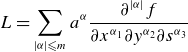 \begin{equation} L = \sum _{\left | \alpha \right |\leqslant m} a^\alpha \frac {\partial ^{\left | \alpha \right |}f}{\partial x^{\alpha _1} \partial y^{\alpha _2} \partial s^{\alpha _3}} \end{equation}
is bounded from $(\sigma ,H^{q+m})$
-analytic functions to
$(\sigma ,H^{q+m})$
-analytic functions to $(\sigma ',H^q)$
-analytic functions.
$(\sigma ',H^q)$
-analytic functions.
Corollary A.5.
Let $\boldsymbol r_0$
be
$\boldsymbol r_0$
be $\mathcal{C}^{4+q}$
for
$\mathcal{C}^{4+q}$
for $q \geqslant 0$
and
$q \geqslant 0$
and $\ell ',\kappa \gt 0$
. There exists a
$\ell ',\kappa \gt 0$
. There exists a $\Sigma \gt 0$
such that the Laplacian, defined in
$\Sigma \gt 0$
such that the Laplacian, defined in $(x,y,s)$
-coordinates via the left-hand side of (2.23), is a bounded operator from
$(x,y,s)$
-coordinates via the left-hand side of (2.23), is a bounded operator from $(\sigma ,H^{q+2})$
to
$(\sigma ,H^{q+2})$
to $(\sigma ',H^q)$
. Similarly, the divergence operator, defined in
$(\sigma ',H^q)$
. Similarly, the divergence operator, defined in $(x,y,s)$
coordinates via the right-hand side of (2.23), is a bounded operator from
$(x,y,s)$
coordinates via the right-hand side of (2.23), is a bounded operator from $(\sigma ,H^{q+1})$
to
$(\sigma ,H^{q+1})$
to $(\sigma ',H^q)$
.
$(\sigma ',H^q)$
.
Proof.
In $(x,y,s)$
-coordinates, we have
$(x,y,s)$
-coordinates, we have $h_s=1-\kappa x$
,
$h_s=1-\kappa x$
, $\sqrt {g}=\ell 'h_s$
and
$\sqrt {g}=\ell 'h_s$
and
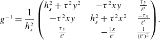 \begin{equation} g^{-1} = \frac {1}{h_s^2}\left(\begin{array}{c@{\quad}c@{\quad}c} h_s^2 + \tau ^2y^2 & - \tau ^2x y & \frac {\tau y}{\ell '} \\[3pt] -\tau ^2 xy & h_s^2 + \tau ^2 x^2 & \frac {-\tau x}{\ell '} \\[3pt] \frac {\tau y}{\ell '} & -\frac {\tau x}{\ell '} & \frac {1}{(\ell ')^2} \end{array}\right)\!. \end{equation}
Because $\boldsymbol r_0 \in \mathcal{C}^{4+q}$
,
$\boldsymbol r_0 \in \mathcal{C}^{4+q}$
, $\ell ' \in \mathcal{C}^{3+q}$
,
$\ell ' \in \mathcal{C}^{3+q}$
, $\kappa \in \mathcal{C}^{2+q}$
and
$\kappa \in \mathcal{C}^{2+q}$
and $\tau \in \mathcal{C}^{1+q}$
, so
$\tau \in \mathcal{C}^{1+q}$
, so $g^{-1} \in \mathcal{C}^{1+q}$
. This means the elements of
$g^{-1} \in \mathcal{C}^{1+q}$
. This means the elements of $h_s^2 g^{-1}$
are
$h_s^2 g^{-1}$
are $(\sigma ,\mathcal{C}^{1+q})$
-analytic with finite series. To include the factor of
$(\sigma ,\mathcal{C}^{1+q})$
-analytic with finite series. To include the factor of $h_s^{-2}$
, we have
$h_s^{-2}$
, we have
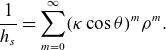 \begin{equation} \frac {1}{h_s} = \sum _{m=0}^{\infty }(\kappa \cos \theta )^m \rho ^m. \end{equation}
The function $\kappa \cos \theta$
is in
$\kappa \cos \theta$
is in $\mathcal{C}^{2+q}$
, so
$\mathcal{C}^{2+q}$
, so $\left \lVert (\kappa \cos \theta )^m \right \rVert _{H^{2+q}} \leqslant C^m \left \lVert \kappa \cos \theta \right \rVert _{\mathcal{C}^{2+q}}^m$
for some
$\left \lVert (\kappa \cos \theta )^m \right \rVert _{H^{2+q}} \leqslant C^m \left \lVert \kappa \cos \theta \right \rVert _{\mathcal{C}^{2+q}}^m$
for some $C\geqslant 1$
and
$C\geqslant 1$
and $h_s^{-1}$
is
$h_s^{-1}$
is $(\Sigma ,\mathcal{C}^{2+q})$
for some
$(\Sigma ,\mathcal{C}^{2+q})$
for some $0\lt \Sigma \leqslant \left \lVert \kappa \right \rVert ^{-1}_{C^0}$
. Finally, after performing the chain rule to bring the operator to the form in Lemma (A.4), the coefficients are each in
$0\lt \Sigma \leqslant \left \lVert \kappa \right \rVert ^{-1}_{C^0}$
. Finally, after performing the chain rule to bring the operator to the form in Lemma (A.4), the coefficients are each in $(\Sigma , H^{q})$
-analytic, giving the result. The same argument applies to the divergence operator.
$(\Sigma , H^{q})$
-analytic, giving the result. The same argument applies to the divergence operator.
The last ingredient needed for the proof of ill-posedness is Cauchy’s estimates for harmonic functions.
Theorem A.6 (Cauchy’s estimates (Axler et al. Reference Axler, Bourdon and Ramey2001)). Let $\alpha = (\alpha _1,\alpha _2, \ldots , \alpha _d)$
be a multi-index. Then, for some constant
$\alpha = (\alpha _1,\alpha _2, \ldots , \alpha _d)$
be a multi-index. Then, for some constant $C_\alpha \gt 0$
, all harmonic functions
$C_\alpha \gt 0$
, all harmonic functions $\phi$
bounded by
$\phi$
bounded by $M$
on the radius-
$M$
on the radius- $R$
ball
$R$
ball $B(x,R)$
satisfy the inequality
$B(x,R)$
satisfy the inequality
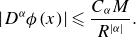 \begin{equation} \left | D^\alpha \phi (x) \right | \leqslant \frac {C_\alpha M}{R^{\left | \alpha \right |}}. \end{equation}
Now, we return to the proof of Theorem (3.6). It is sufficient to show that $\phi$
is not
$\phi$
is not $(\sigma ,H^q)$
-analytic for
$(\sigma ,H^q)$
-analytic for $q = 2$
. So, consider input data such that
$q = 2$
. So, consider input data such that $\left \lVert \phi \right \rVert _{\sigma ,H^2} \lt \infty$
, say constructed via Proposition (3.2). We will focus on perturbations in
$\left \lVert \phi \right \rVert _{\sigma ,H^2} \lt \infty$
, say constructed via Proposition (3.2). We will focus on perturbations in $B_0$
of the form
$B_0$
of the form $\Delta B_0^{(j)} = c_j e^{{\mathrm{i}} j s}$
, where
$\Delta B_0^{(j)} = c_j e^{{\mathrm{i}} j s}$
, where $c_j = j^{-N}$
and
$c_j = j^{-N}$
and $N\gt q_0+1$
is a positive integer, while
$N\gt q_0+1$
is a positive integer, while $\boldsymbol r_0$
and
$\boldsymbol r_0$
and $\phi ^{(\text{IC})}$
remain constant. Clearly,
$\phi ^{(\text{IC})}$
remain constant. Clearly, $\left \lVert \Delta B_0 \right \rVert _{H^{1+q_0}} \to 0$
as
$\left \lVert \Delta B_0 \right \rVert _{H^{1+q_0}} \to 0$
as $j\to \infty$
. Let
$j\to \infty$
. Let $\phi ^{(j)}$
be the formal power series solution of the perturbed problem.
$\phi ^{(j)}$
be the formal power series solution of the perturbed problem.
We want to show that $\phi ^{(j)}$
cannot converge to a
$\phi ^{(j)}$
cannot converge to a $(\sigma ,H^q)$
-analytic solution. In the case where the perturbed near-axis expansion for fixed
$(\sigma ,H^q)$
-analytic solution. In the case where the perturbed near-axis expansion for fixed $j$
does not converge in
$j$
does not converge in $\Omega _\sigma$
, then
$\Omega _\sigma$
, then $\left \lVert \phi ^{(j)} \right \rVert _{\sigma ,H^2} = \infty$
for all
$\left \lVert \phi ^{(j)} \right \rVert _{\sigma ,H^2} = \infty$
for all $\sigma$
and we are done, as the operator fails to be bounded for a specific function. Otherwise, suppose the near-axis expansion solution converges on
$\sigma$
and we are done, as the operator fails to be bounded for a specific function. Otherwise, suppose the near-axis expansion solution converges on $\Omega _\sigma$
and each
$\Omega _\sigma$
and each $\phi ^{(j)}$
is
$\phi ^{(j)}$
is $(\sigma ,H^2)$
-analytic. Then, using Corollary (13), for
$(\sigma ,H^2)$
-analytic. Then, using Corollary (13), for $\sigma '\lt \sigma$
,
$\sigma '\lt \sigma$
, $\Delta \phi ^{(j)} + \nabla \cdot \tilde {\boldsymbol{B}}$
is a
$\Delta \phi ^{(j)} + \nabla \cdot \tilde {\boldsymbol{B}}$
is a $(\sigma ',L^2)$
-analytic function. Because
$(\sigma ',L^2)$
-analytic function. Because $\phi$
satisfies the near-axis expansion, the solution must satisfy
$\phi$
satisfies the near-axis expansion, the solution must satisfy $(\Delta \phi ^{(j)}+\nabla \cdot \tilde {\boldsymbol{B}})_m =0$
in
$(\Delta \phi ^{(j)}+\nabla \cdot \tilde {\boldsymbol{B}})_m =0$
in $L^2(\mathbb{T}^2)$
, further implying that
$L^2(\mathbb{T}^2)$
, further implying that $\Delta \phi ^{(j)}+\nabla \cdot \tilde {\boldsymbol{B}} = 0$
in
$\Delta \phi ^{(j)}+\nabla \cdot \tilde {\boldsymbol{B}} = 0$
in $L^2(\Omega _{\sigma '}^0)$
. Pulling this back to
$L^2(\Omega _{\sigma '}^0)$
. Pulling this back to $\Omega _{\sigma '}$
, we are solving the standard Poisson’s equation
$\Omega _{\sigma '}$
, we are solving the standard Poisson’s equation $\Delta \phi ^{(j)} = -\nabla \cdot \tilde {\boldsymbol{B}}$
in
$\Delta \phi ^{(j)} = -\nabla \cdot \tilde {\boldsymbol{B}}$
in $L^2(\Omega _{\sigma '})$
. If we locally define
$L^2(\Omega _{\sigma '})$
. If we locally define
 \begin{equation} \psi ^{(j)} = \phi ^{(j)} + \int _0^s B_0(s')\ell '(s') \hspace {1pt} \mathrm{d} s', \end{equation}
we find $\Delta \psi ^{(j)} = 0$
. That is,
$\Delta \psi ^{(j)} = 0$
. That is, $\psi ^{(j)}$
is analytic in simply connected subdomains of
$\psi ^{(j)}$
is analytic in simply connected subdomains of $\Omega _{\sigma '}$
and the magnetic field is locally the gradient of
$\Omega _{\sigma '}$
and the magnetic field is locally the gradient of $\psi ^{(j)}$
.
$\psi ^{(j)}$
.
Then, let $B(x,R)$
be a ball around a point on the magnetic axis
$B(x,R)$
be a ball around a point on the magnetic axis $\boldsymbol r_0(s_0)$
. At
$\boldsymbol r_0(s_0)$
. At $\boldsymbol r_0(s_0)$
, the order
$\boldsymbol r_0(s_0)$
, the order $M\gt N$
derivative in the tangent direction of
$M\gt N$
derivative in the tangent direction of $\boldsymbol r_0$
of
$\boldsymbol r_0$
of $\psi ^{(j)}$
takes the polynomial form
$\psi ^{(j)}$
takes the polynomial form
 \begin{equation} \frac {\partial ^M\psi ^{(j)}}{\partial s^M} = \frac {\partial ^M B_0}{\partial s^M} + c_j \sum _{\ell = 0}^M a_\ell j^\ell , \end{equation}
where $a_{M} = ({\mathrm{i}} / \ell '(s_0))^{M} e^{{\mathrm{i}} j s_0} \neq 0$
and
$a_{M} = ({\mathrm{i}} / \ell '(s_0))^{M} e^{{\mathrm{i}} j s_0} \neq 0$
and $a_\ell$
for
$a_\ell$
for $\ell \lt M$
contain higher order derivatives of the axis. As such, there is a
$\ell \lt M$
contain higher order derivatives of the axis. As such, there is a $J$
such that
$J$
such that $j \gt J$
implies that
$j \gt J$
implies that
 \begin{equation} \left | \frac {\partial ^M\psi ^{(j)}}{\partial s^M} \right | \gt \frac {\left | a_N \right |}{2} j^{M-N}. \end{equation}
Then, by Theorem (A.6), we have that
 \begin{equation} \max _{B(x,R)} \psi ^{(j)} \gt \frac {R^N a_N}{2 C_N} j^{M-N}. \end{equation}
So, as $j \to \infty$
,
$j \to \infty$
, $\psi ^{(j)}$
cannot converge to a continuous function. However, because
$\psi ^{(j)}$
cannot converge to a continuous function. However, because $\phi$
was assumed
$\phi$
was assumed $(\sigma ,H^2)$
-analytic and by Corollary (3.5) it must be continuous, we have drawn a contradiction.
$(\sigma ,H^2)$
-analytic and by Corollary (3.5) it must be continuous, we have drawn a contradiction.
A.4 Proof of Theorem (3.8)
We will start with two lemmas. The first is on the boundedness of the right-hand-side operator of the PDE (3.20).
Lemma A.7.
Let $q\geqslant 0$
,
$q\geqslant 0$
, $D\geqslant 1$
,
$D\geqslant 1$
, $0\lt \sigma \leqslant \sigma _0 \lt \Sigma$
,
$0\lt \sigma \leqslant \sigma _0 \lt \Sigma$
, $\phi$
be
$\phi$
be $(\sigma ,H^{q+2D})$
-analytic, and
$(\sigma ,H^{q+2D})$
-analytic, and $a^{(j)}$
be
$a^{(j)}$
be $(\Sigma ,\mathcal{C}^q)$
-analytic for
$(\Sigma ,\mathcal{C}^q)$
-analytic for $1\leqslant j \leqslant 7$
. Then, the operator
$1\leqslant j \leqslant 7$
. Then, the operator $L^{(a)}$
defined in (3.21) preserves the analytic form (3.4) and satisfies the bound
$L^{(a)}$
defined in (3.21) preserves the analytic form (3.4) and satisfies the bound
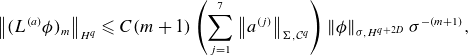 \begin{equation} \left \lVert (L^{(a)}\phi )_m \right \rVert _{H^q} \leqslant C (m+1) \left (\sum _{j=1}^7 \left \lVert a^{(j)} \right \rVert _{\Sigma ,\mathcal{C}^q} \right ) \left \lVert \phi \right \rVert _{\sigma ,H^{q+2D}} \sigma ^{-(m+1)}, \end{equation}
where $C$
depends on
$C$
depends on $\sigma _0$
but not on
$\sigma _0$
but not on $\sigma$
.
$\sigma$
.
Proof.
For $j\neq 2$
, Lemmas (A.2) and (A.3) tell us that
$j\neq 2$
, Lemmas (A.2) and (A.3) tell us that
 \begin{equation} L^{(\neq 2)}\phi = a^{(1)}\phi + a^{(3)} \frac {\partial \phi }{\partial \theta } + a^{(4)} \frac {\partial \phi }{\partial s} + a^{(5)} \frac {\partial ^2\phi }{\partial \theta ^2} + a^{(6)} \frac {\partial ^2\phi }{\partial \theta \partial s} + a^{(7)} \frac {\partial ^2 \phi }{\partial s^2} \end{equation}
satisfies the analytic form and has the bound
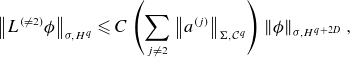 \begin{equation} \left \lVert L^{(\neq 2)}\phi \right \rVert _{\sigma ,H^{q}} \leqslant C \left (\sum _{j\neq 2}\left \lVert a^{(j)} \right \rVert _{\Sigma ,\mathcal{C}^q}\right ) \left \lVert \phi \right \rVert _{\sigma ,H^{q+2D}}, \end{equation}
where $C$
does not depend on
$C$
does not depend on $\sigma$
.
$\sigma$
.
For the $j=2$
term, define
$j=2$
term, define
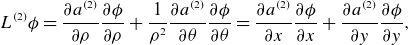 \begin{equation} L^{(2)}\phi = \frac {\partial a^{(2)}}{\partial \rho } \frac {\partial \phi }{\partial \rho } + \frac {1}{\rho ^2} \frac {\partial a^{(2)}}{\partial \theta }\frac {\partial \phi }{\partial \theta }= \frac {\partial a^{(2)}}{\partial x} \frac {\partial \phi }{\partial x} + \frac {\partial a^{(2)}}{\partial y}\frac {\partial \phi }{\partial y}, \end{equation}
where $x = \rho \cos \theta$
and
$x = \rho \cos \theta$
and $y = \rho \sin \theta$
. By Lemmas (A.1) and (A.3), this preserves the analytic form. To bound the operator, first note that
$y = \rho \sin \theta$
. By Lemmas (A.1) and (A.3), this preserves the analytic form. To bound the operator, first note that
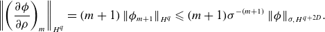 \begin{equation} \left \lVert \left (\frac {\partial \phi }{\partial \rho }\right )_m \right \rVert _{H^q} = (m+1) \left \lVert \phi _{m+1} \right \rVert _{H^{q}} \leqslant (m+1) \sigma ^{-(m+1)} \left \lVert \phi \right \rVert _{\sigma ,H^{q+2D}}\!. \end{equation}
A similar bound is satisfied by the $\theta$
derivative:
$\theta$
derivative:
 \begin{equation} \left \lVert \left (\frac {\partial \phi }{\partial \theta }\right )_m \right \rVert _{H^q} \leqslant m \sigma ^{-m} \left \lVert \phi \right \rVert _{\sigma ,H^{q+2D}}\,. \end{equation}
So, we focus on the $\rho$
derivative term of
$\rho$
derivative term of $L^{(2)}$
, where the same steps can be used to bound the
$L^{(2)}$
, where the same steps can be used to bound the $\theta$
derivative term. We have that
$\theta$
derivative term. We have that
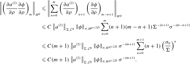 \begin{align} \left \lVert \left (\frac {\partial a^{(2)}}{\partial \rho } \frac {\partial \phi }{\partial \rho } \right )_m \right \rVert _{H^q} &\leqslant \left \lVert \sum _{n=0}^m \left (\frac {\partial a^{(2)}}{\partial \rho }\right )_{n+1} \left (\frac {\partial \phi }{\partial \rho }\right )_{m-n+1} \right \rVert _{H^q} \nonumber \\ &\leqslant C \left \lVert a^{(2)} \right \rVert _{\Sigma ,\mathcal{C}^q} \left \lVert \phi \right \rVert _{\sigma ,H^{q+2D}} \sum _{n=0}^m (n+1)(m-n+1) \Sigma ^{-(n+1)} \sigma ^{-(m-n+1)} \nonumber \\ & \leqslant C (m+1) \left \lVert a^{(2)} \right \rVert _{\Sigma ,\mathcal{C}^q} \left \lVert \phi \right \rVert _{\sigma ,H^{q+2D}} \sigma ^{-(m+1)} \sum _{n=0}^{m+1} (n+1) \left (\frac {\sigma _0}{\Sigma }\right )^n\nonumber \\ & \leqslant C (m+1) \left \lVert a^{(2)} \right \rVert _{\Sigma ,\mathcal{C}^q} \left \lVert \phi \right \rVert _{\sigma ,H^{q+2D}} \sigma ^{-(m+1)}. \end{align}
Combining the estimates on $L^{(2)}$
and
$L^{(2)}$
and $L^{(\neq 2)}$
, we have our theorem.
$L^{(\neq 2)}$
, we have our theorem.
Then, the main step in proving Theorem (3.8) is to show the inductive step in Lemma (A.9). For this, we depend on the following interior regularity theorem for the regularisation.
Theorem A.8 ((Taylor (Reference Taylor2011), Theorem 11.1)). If $P$
is elliptic of order
$P$
is elliptic of order $2 D$
and
$2 D$
and $u\in \mathcal{D}'(M)$
,
$u\in \mathcal{D}'(M)$
, $Pu = h \in H^{q}(M)$
, then
$Pu = h \in H^{q}(M)$
, then $u\in H_{\mathrm{loc}}^{q+2D}(M)$
, and, for each
$u\in H_{\mathrm{loc}}^{q+2D}(M)$
, and, for each $U \subset \subset V \subset \subset M$
,
$U \subset \subset V \subset \subset M$
, $\sigma \lt q+2D$
, there is an estimate
$\sigma \lt q+2D$
, there is an estimate
 \begin{equation} \left \lVert u \right \rVert _{H^{q+2D}(U)} \leqslant C \left \lVert P u \right \rVert _{H^{q}(V)} + C \left \lVert u \right \rVert _{H^\sigma (V)}. \end{equation}
Then, our inductive step is the following lemma.
Lemma A.9.
Assume the hypotheses of Theorem (3.8), and let $\sigma \leqslant \sigma _0 \leqslant \sigma ' \lt \Sigma$
and
$\sigma \leqslant \sigma _0 \leqslant \sigma ' \lt \Sigma$
and $m\geqslant 0$
. Suppose we have computed the finite solution
$m\geqslant 0$
. Suppose we have computed the finite solution
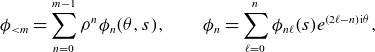 \begin{equation} \phi _{\lt m} = \sum _{n=0}^{m-1}\rho ^n \phi _n(\theta ,s), \qquad \phi _n = \sum _{\ell = 0}^{n} \phi _{n\ell }(s) e^{(2\ell -n){\mathrm{i}} \theta }, \end{equation}
where
 \begin{equation} \left \lVert \phi _n \right \rVert _{H^{q+2D}} \lt \Phi \sigma ^{-n} \qquad \text{ for all } n\lt m. \end{equation}
Then,
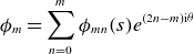 \begin{equation} \phi _m = \sum _{n=0}^m \phi _{mn}(s) e^{(2n-m){\mathrm{i}}\theta } \end{equation}
and there exists two constants $C_1, C_2 \gt 0$
independent of
$C_1, C_2 \gt 0$
independent of $m$
,
$m$
, $\sigma$
,
$\sigma$
, $\sigma _0$
,
$\sigma _0$
, $\phi ^{(\text{IC})}$
,
$\phi ^{(\text{IC})}$
, $f$
and
$f$
and $\Phi$
, where
$\Phi$
, where $C_1$
depends continuously on
$C_1$
depends continuously on $a^{(j)}$
and
$a^{(j)}$
and $\sigma '$
, and
$\sigma '$
, and $C_2$
is independent of
$C_2$
is independent of $a^{(j)}$
such that
$a^{(j)}$
such that
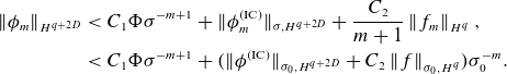 \begin{align} \left \lVert \phi _m \right \rVert _{H^{q+2D}} &\lt C_{1} \Phi \sigma ^{-m+1} + \lVert \phi ^{(\text{IC})}_m\rVert _{\sigma ,H^{q+2D}} + \frac {C_2}{m+1} \left \lVert f_m \right \rVert _{H^q},\nonumber \\ &\lt C_{1} \Phi \sigma ^{-m+1} + (\lVert \phi ^{(\text{IC})}\rVert _{\sigma _0,H^{q+2D}} + C_2 \left \lVert f \right \rVert _{\sigma _0,H^q}) \sigma _0^{-m}. \end{align}
Proof.
Let $L^{(a)}$
be as in (3.21). Then, the near-axis iteration is given by
$L^{(a)}$
be as in (3.21). Then, the near-axis iteration is given by
 \begin{equation} \phi _m = \phi ^{(\text{IC})}_m + ((1+P)^{-1} \Delta _\perp ^{+} (f+L^{(a)}\phi _{\lt m}))_m, \end{equation}
where $\Delta _\perp ^+$
is defined in (3.24). As such, the triangle inequality gives
$\Delta _\perp ^+$
is defined in (3.24). As such, the triangle inequality gives
 \begin{equation} \left \lVert \phi _m \right \rVert _{H^{q+2D}} \leqslant \left \lVert \phi ^{(\text{IC})}_m \right \rVert _{H^{q+2D}} + \left \lVert (1+P)^{-1} (\Delta _\perp ^{+} (f+L^{(a)}\phi _{\lt m}))_m \right \rVert _{H^{q+2D}}. \end{equation}
For the initial conditions, we have
 \begin{equation} \left \lVert \phi ^{(\text{IC})}_m \right \rVert _{H^{q+2D}} \leqslant \left \lVert \phi ^{(\text{IC})}_m \right \rVert _{\sigma _0,H^{q+2D}} \sigma _0^{-m}, \end{equation}
so we just need to focus on the second term.
Let $g = f + L^{(a)} \phi _{\lt m}$
. By Lemma (A.7), we have that
$g = f + L^{(a)} \phi _{\lt m}$
. By Lemma (A.7), we have that
 \begin{equation} \left \lVert g_m \right \rVert _{H^q} \leqslant \left \lVert f \right \rVert _{\sigma _0,H^q}\sigma _0^{-m} + C (m+1) \left (\sum _{j=1}^7 \left \lVert a^{(j)} \right \rVert _{\Sigma ,\mathcal{C}^q} \right ) \Phi \sigma ^{-(m+1)}, \end{equation}
where $C$
depends on
$C$
depends on $\sigma '$
and we have used
$\sigma '$
and we have used $\left \lVert \phi _{\lt m} \right \rVert _{\sigma ,H^q} \leqslant \Phi$
. Next, we establish a bound for the inverse polar Laplacian. We have that
$\left \lVert \phi _{\lt m} \right \rVert _{\sigma ,H^q} \leqslant \Phi$
. Next, we establish a bound for the inverse polar Laplacian. We have that
 \begin{equation} \left (\Delta _\perp ^{+}g\right )_m = \sum _{n=1}^{m-1} \frac {1}{m^2 - (2n-m)^2}g_{m-2,n-1} e^{(2n-m){\mathrm{i}} \theta }, \end{equation}
so for $m\geqslant 2$
,
$m\geqslant 2$
,
 \begin{align} \left \lVert \left (\Delta _\perp ^{+}g\right )_m \right \rVert ^2_{H^{q}} =& \sum _{n=1}^{m-1} \frac {1}{m^2 - (2n-m)^2}\left \lVert g_{m-2,n-1} e^{(2n-m){\mathrm{i}} \theta } \right \rVert ^2_{H^{q}}\!, \nonumber \\ \leqslant & \frac {1}{4(m-1)} \sum _{n=1}^{m-1} \left \lVert g_{m-2,n-1} e^{(2n-m){\mathrm{i}} \theta } \right \rVert ^2_{H^{q}}\!,\nonumber \\ =& \frac {1}{4(m-1)}\left \lVert g_{m-2} \right \rVert ^2_{H^{q}}\!,\nonumber \\ \leqslant & \frac {C^{(1)}}{m+1} \left \lVert f \right \rVert _{\sigma _0,H^q}\sigma _0^{-m} + C^{(2)} \left (\sum _{j=1}^7 \left \lVert a^{(j)} \right \rVert _{\Sigma ,\mathcal{C}^q} \right ) \Phi \sigma ^{-m+1}, \end{align}
where we used constants so that this is trivially extended to $m \in \{0,1\}$
, where
$m \in \{0,1\}$
, where $(\Delta _\perp ^+ g)_0 = (\Delta _\perp ^+ g)_1 = 0$
.
$(\Delta _\perp ^+ g)_0 = (\Delta _\perp ^+ g)_1 = 0$
.
Now, we would like to bound the inverse operator $(1+P)^{-1}$
. Specifically, we need it to be the case that
$(1+P)^{-1}$
. Specifically, we need it to be the case that
 \begin{equation} \left \lVert u \right \rVert _{H^{q+2D}} \lt C \left \lVert (1+P) u \right \rVert _{H^{q}}\!. \end{equation}
We will prove this is true by the standard argument. For the sake of contradiction, suppose that there exists a sequence $u^{(n)} \in H^{q + 2 D}$
such that
$u^{(n)} \in H^{q + 2 D}$
such that $\left \lVert u^{(n)} \right \rVert _{L^2} = 1$
and
$\left \lVert u^{(n)} \right \rVert _{L^2} = 1$
and $\left \lVert (1+P) u^{(n)} \right \rVert _{H^{q}} \to 0$
. By Theorem (A.8), this tells us that
$\left \lVert (1+P) u^{(n)} \right \rVert _{H^{q}} \to 0$
. By Theorem (A.8), this tells us that $\left \lVert u^{(n)} \right \rVert _{H^{q+2D}}\leqslant 1 + \epsilon$
for some
$\left \lVert u^{(n)} \right \rVert _{H^{q+2D}}\leqslant 1 + \epsilon$
for some $\epsilon \gt 0$
. By Rellich’s theorem (Taylor Reference Taylor2011, Proposition 3.4),
$\epsilon \gt 0$
. By Rellich’s theorem (Taylor Reference Taylor2011, Proposition 3.4), $H^{q + 2D}$
is compactly embedded in
$H^{q + 2D}$
is compactly embedded in $H^{q+2D-1}$
, so there exists a subsequence such that
$H^{q+2D-1}$
, so there exists a subsequence such that $u_{n} \to u$
in
$u_{n} \to u$
in $H^{q+2D-1}$
. This implies that
$H^{q+2D-1}$
. This implies that $(1+P) u^{(n)} \to (1+P) u = 0$
in
$(1+P) u^{(n)} \to (1+P) u = 0$
in $H^{q-1}$
, where we are using the assumption that
$H^{q-1}$
, where we are using the assumption that $q\geqslant 1$
. However, because
$q\geqslant 1$
. However, because $1+P$
is positive, it does not have a kernel, so the bound (A.37) must hold.
$1+P$
is positive, it does not have a kernel, so the bound (A.37) must hold.
Equation (A.37) tells us that $1+P$
is one-to-one from
$1+P$
is one-to-one from $H^{q+2D}$
to
$H^{q+2D}$
to $H^q$
. Moreover, because
$H^q$
. Moreover, because $1+P$
is positive and self-adjoint, it must be surjective, so it is invertible and we have the inequality
$1+P$
is positive and self-adjoint, it must be surjective, so it is invertible and we have the inequality
 \begin{equation} \left \lVert (1+P)^{-1}\left (\Delta _\perp ^{+}g\right )_m \right \rVert ^2_{H^{q+2D}} \leqslant \frac {C_1}{m+1} \left \lVert f \right \rVert _{\sigma _0,H^q}\sigma _0^{-m} + C_2 \left (\sum _{j=1}^7 \left \lVert a^{(j)} \right \rVert _{\Sigma ,\mathcal{C}^q} \right ) \Phi \sigma ^{-m+1}, \end{equation}
proving the lemma.
We are now ready to prove Theorem (3.8). For continuity (boundedness) of the solution with respect to $\phi ^{(\text{IC})}$
and
$\phi ^{(\text{IC})}$
and $f$
, we choose a
$f$
, we choose a $\sigma$
such that
$\sigma$
such that $\sigma C_1 \lt 1$
and
$\sigma C_1 \lt 1$
and $\sigma \leqslant \sigma _0$
. Then, let
$\sigma \leqslant \sigma _0$
. Then, let $0 \lt \gamma \lt 1 - C_1 \sigma$
. We choose
$0 \lt \gamma \lt 1 - C_1 \sigma$
. We choose $\Phi$
such that
$\Phi$
such that
 \begin{equation} C_1 \sigma \Phi + \left \lVert \phi ^{(\text{IC})} \right \rVert _{\sigma ,H^{q+2D}} + C_2 \left \lVert f \right \rVert _{\sigma _0,H^q} = (1-\gamma ) \Phi . \end{equation}
Then, we perform induction. At $m=0$
,
$m=0$
, $\phi _{\lt m} = 0$
, so we have trivially satisfied the initial case. For the inductive step, because
$\phi _{\lt m} = 0$
, so we have trivially satisfied the initial case. For the inductive step, because $\sigma _0^{-m}\leqslant \sigma ^{-m}$
, we have
$\sigma _0^{-m}\leqslant \sigma ^{-m}$
, we have
 \begin{equation} \left \lVert \phi _m \right \rVert _{H^{q+2D}} \leqslant (1-\gamma )\Phi \sigma ^{-m}, \end{equation}
implying
 \begin{equation} \left \lVert \phi \right \rVert _{\sigma , H^{q+2D}} \leqslant \Phi = \frac {1-\gamma }{1-\gamma - C_1 \sigma }\left (\left \lVert \phi ^{(\text{IC})} \right \rVert _{\sigma ,H^{q+2D}} + C_2 \left \lVert f \right \rVert _{\sigma _0,H^q} \right ). \end{equation}
For continuity with respect to the coefficients $A = (a^{(1)}, \ldots , a^{(7)})$
, consider fixing
$A = (a^{(1)}, \ldots , a^{(7)})$
, consider fixing $\sigma$
and
$\sigma$
and $\gamma$
as before. Then, because
$\gamma$
as before. Then, because $C_1$
is continuous with respect to
$C_1$
is continuous with respect to $A$
, there is a small enough perturbation so that both
$A$
, there is a small enough perturbation so that both $\sigma$
and
$\sigma$
and $\gamma$
continue to satisfy
$\gamma$
continue to satisfy $0 \lt \gamma \lt 1-C_1 \sigma$
and
$0 \lt \gamma \lt 1-C_1 \sigma$
and $C_1 \sigma \lt 1$
. So, there is a neighbourhood of
$C_1 \sigma \lt 1$
. So, there is a neighbourhood of $U$
of
$U$
of $A$
such that for all
$A$
such that for all $A+\delta A \in U$
and some values of
$A+\delta A \in U$
and some values of $C$
, we have
$C$
, we have $\left \lVert \phi \right \rVert _{\sigma ,H^{q+2D}} \leqslant C (\lVert \phi ^{(\text{IC})} \rVert _{\sigma _0,H^{q+2D}} + \left \lVert f \right \rVert _{\sigma _0,H^{q}})$
. Because
$\left \lVert \phi \right \rVert _{\sigma ,H^{q+2D}} \leqslant C (\lVert \phi ^{(\text{IC})} \rVert _{\sigma _0,H^{q+2D}} + \left \lVert f \right \rVert _{\sigma _0,H^{q}})$
. Because $C_1$
does not depend on
$C_1$
does not depend on $\sigma _0$
, it is also the case that there is a neighbourhood of
$\sigma _0$
, it is also the case that there is a neighbourhood of $U_0$
of
$U_0$
of $A$
such that
$A$
such that $\left \lVert \phi \right \rVert _{\sigma ,H^{q+2D}}\leqslant C_0 (\lVert \phi ^{(\text{IC})} \rVert _{\sigma ,H^{q+2D}} + \left \lVert f \right \rVert _{\sigma _0,H^{q}})$
for all
$\left \lVert \phi \right \rVert _{\sigma ,H^{q+2D}}\leqslant C_0 (\lVert \phi ^{(\text{IC})} \rVert _{\sigma ,H^{q+2D}} + \left \lVert f \right \rVert _{\sigma _0,H^{q}})$
for all $A+\delta A \in U_0$
.
$A+\delta A \in U_0$
.
Now, consider the full PDE operator
 \begin{equation} L = \Delta _\perp (1+P) - L^{(a)}, \end{equation}
and let $L+\delta L$
be the operator associated with substituting
$L+\delta L$
be the operator associated with substituting $a^{(j)}$
with
$a^{(j)}$
with $a^{(j)}+\delta a^{(j)}\in U \cap U_0$
, i.e.
$a^{(j)}+\delta a^{(j)}\in U \cap U_0$
, i.e.
 \begin{align} \delta L\phi = \delta L^{(a)}\phi = \delta a^{(1)}\phi & + \frac {\partial (\delta a^{(2)})}{\partial \rho } \frac {\partial \phi }{\partial \rho } + \frac {1}{\rho ^2} \frac {\partial (\delta a^{(2)})}{\partial \theta }\frac {\partial \phi }{\partial \theta }\nonumber\\ &+ \delta a^{(3)} \frac {\partial \phi }{\partial \theta }+ \delta a^{(4)} \frac {\partial \phi }{\partial s} + \delta a^{(5)} \frac {\partial ^2\phi }{\partial \theta ^2} + \delta a^{(6)} \frac {\partial ^2\phi }{\partial \theta \partial s} + \delta a^{(7)} \frac {\partial ^2 \phi }{\partial s^2}. \end{align}
With fixed initial conditions $\phi ^{(\text{IC})}$
and
$\phi ^{(\text{IC})}$
and $f$
, let the solution to the original PDE be
$f$
, let the solution to the original PDE be $\phi$
(i.e.
$\phi$
(i.e. $L \phi = f$
) and the solution to the perturbed PDE be
$L \phi = f$
) and the solution to the perturbed PDE be $\phi + \delta \phi$
(i.e.
$\phi + \delta \phi$
(i.e. $(L+\delta L)(\phi + \delta \phi ) = f$
). Subtracting the two PDE formulae gives
$(L+\delta L)(\phi + \delta \phi ) = f$
). Subtracting the two PDE formulae gives
 \begin{equation} (L+\delta L)\delta \phi = -\delta L \phi , \end{equation}
where $\delta \phi$
satisfies
$\delta \phi$
satisfies $\delta \phi ^{(\text{IC})} = 0$
. Using Lemma (A.7), we have that
$\delta \phi ^{(\text{IC})} = 0$
. Using Lemma (A.7), we have that
 \begin{equation} \left \lVert (\delta L \phi )_m \right \rVert _{H^q} \leqslant C (m+1) \left (\sum _{j=1}^7 \left \lVert \delta a^{(j)} \right \rVert _{\Sigma ,\mathcal{C}^q} \right ) \left \lVert \phi \right \rVert _{\sigma ,H^{q+2D}} \sigma ^{-m}. \end{equation}
Then, we find that
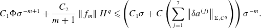 \begin{equation} C_1 \Phi \sigma ^{-m+1} + \frac {C_2}{m+1}\left \lVert f_m \right \rVert {H^q} \leqslant \left (C_1 \sigma + C \left (\sum _{j=1}^7 \left \lVert \delta a^{(j)} \right \rVert _{\Sigma ,\mathcal{C}^q} \right ) \right ) \sigma ^{-m}. \end{equation}
We can take $\delta A$
small enough so the right term is less than
$\delta A$
small enough so the right term is less than $1$
, allowing us to proceed inductively as before, giving continuity in the coefficients.
$1$
, allowing us to proceed inductively as before, giving continuity in the coefficients.
A.5 Proof of Corollary (3.9)
For the coefficients of the PDE, we must only notice that
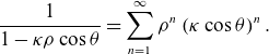 \begin{equation} \frac {1}{1-\kappa \rho \cos \theta } = \sum _{n=1}^{\infty }\rho ^n \left (\kappa \cos \theta \right )^n. \end{equation}
Because $\boldsymbol r_0 \in \mathcal{C}^{4+q}(\mathbb{T})$
,
$\boldsymbol r_0 \in \mathcal{C}^{4+q}(\mathbb{T})$
, $\kappa \in \mathcal{C}^{3+q}(\mathbb{T})$
. This immediately tells us that
$\kappa \in \mathcal{C}^{3+q}(\mathbb{T})$
. This immediately tells us that
 \begin{equation} \left \lVert (\kappa \cos \theta )^n \right \rVert _{\mathcal{C}^{3+q}} \leqslant \left (C \left \lVert \kappa \cos \theta \right \rVert _{\mathcal{C}^{3+q}}\right )^n \end{equation}
for some constant $C$
, showing this converges. (In fact, the sum converges for all
$C$
, showing this converges. (In fact, the sum converges for all $\rho \lt \kappa$
.)
$\rho \lt \kappa$
.)
We note that $P$
satisfies the Hypotheses (3.7) by construction, so we can apply Theorem (3.8). The regularity of
$P$
satisfies the Hypotheses (3.7) by construction, so we can apply Theorem (3.8). The regularity of $\boldsymbol B_K$
is the obtained from (3.18), where the reduction in regularity comes from the order of
$\boldsymbol B_K$
is the obtained from (3.18), where the reduction in regularity comes from the order of $P$
, combined with Lemmas (A.1) and (A.3).
$P$
, combined with Lemmas (A.1) and (A.3).
A.6 Proof of Propsition (3.10)
For the statement about uniqueness, suppose $\phi'\!\in\!H^{q+2D}(\Omega _{\sigma '}^0)$
with
$\phi'\!\in\!H^{q+2D}(\Omega _{\sigma '}^0)$
with $\phi '-\phi =\delta \phi \neq 0$
satisfies the boundary value problem. Then,
$\phi '-\phi =\delta \phi \neq 0$
satisfies the boundary value problem. Then, $\delta \phi$
satisfies
$\delta \phi$
satisfies
 \begin{equation} -(P \Delta _\perp + L)\delta \phi = 0, \qquad \left . \delta \phi \right |_{\rho =\sigma '} = 0. \end{equation}
Then, after some algebra, we have
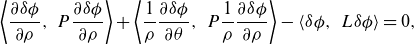 \begin{equation} \left \langle \frac {\partial \delta \phi }{\partial \rho } , \ P \frac {\partial \delta \phi }{\partial \rho } \right \rangle + \left \langle \frac {1}{\rho } \frac {\partial \delta \phi }{\partial \theta } , \ P \frac {1}{\rho } \frac {\partial \delta \phi }{\partial \rho } \right \rangle - \left \langle \delta \phi , \ L \delta \phi \right \rangle = 0, \end{equation}
where the inner product is the $L^2$
inner product
$L^2$
inner product
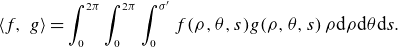 \begin{equation} \left \langle f , \ g \right \rangle = \int _0^{2\pi } \int _{0}^{2\pi } \int _{0}^{\sigma '} f(\rho ,\theta ,s) g(\rho ,\theta ,s) \, \rho \mathrm{d}\rho \mathrm{d}\theta \mathrm{d} s. \end{equation}
By our assumptions on $P$
and
$P$
and $L$
, each term in (A.50) is positive. So, it then must be the case that
$L$
, each term in (A.50) is positive. So, it then must be the case that $\left \langle \delta \phi , \ L\delta \phi \right \rangle = 0$
. However, this is only possible when
$\left \langle \delta \phi , \ L\delta \phi \right \rangle = 0$
. However, this is only possible when $\delta \phi = 0$
, so the solution is unique.
$\delta \phi = 0$
, so the solution is unique.
For the error estimate, fix $\phi$
and subtract the two boundary value problems to find that
$\phi$
and subtract the two boundary value problems to find that
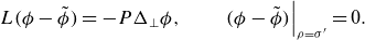 \begin{equation} L(\phi - \tilde \phi ) = - P \Delta _\perp \phi , \qquad \left .(\phi - \tilde \phi )\right |_{\rho = \sigma '} = 0. \end{equation}
Because $L$
is negative, there is a unique solution
$L$
is negative, there is a unique solution $\phi -\tilde \phi$
to this problem. Then, by standard regularity theory (Evans Reference Evans2010, Theorem 6.3.5), we have the desired bound.
$\phi -\tilde \phi$
to this problem. Then, by standard regularity theory (Evans Reference Evans2010, Theorem 6.3.5), we have the desired bound.
Appendix B. Asymptotic expansions of basic operations
To build the near-axis code, we need some facts from formal expansions. We let $A$
,
$A$
, $B$
and
$B$
and $C$
be smooth formal power series of the generic form
$C$
be smooth formal power series of the generic form
 \begin{equation} A(\rho ,\theta ,s) = \sum _{n = 0}^\infty A_n(\theta , s) \rho ^n, \end{equation}
and let $\alpha \in \mathbb{R}$
. Here, we explain how we numerically perform the following basic operations:
$\alpha \in \mathbb{R}$
. Here, we explain how we numerically perform the following basic operations:
-
(i) multiplication (Appendix B.1),
$C=AB$
; -
(ii) multiplicative inversion (Appendix B.2),
$B=A^{-1}$
; -
(iii) differentiation with respect to
$\rho$
(Appendix B.3),
$B = ({\mathrm{d} A}/{\mathrm{d} \rho })$
; -
(iv) exponentiation (Appendix B.4),
$B = e^{\alpha A}$
; -
(v) power (Appendix B.5),
$B = A^{\alpha }$
; -
(vi) composition (Appendix B.6),
$A(\tilde \rho , \tilde \theta , \phi )$
where
$\begin{pmatrix} B & \kern6pt C\end{pmatrix}^T = \begin{pmatrix} \tilde \rho \cos \tilde \theta & \kern6pt \tilde \rho \sin \tilde \theta \end{pmatrix}^T$
; -
(vii) series inversion (Appendix B.6), find the inverse coordinate transformation
$C^{(i)}$
of the transformation
$B{(i)}$
, i.e.(B.2)
\begin{equation} \begin{pmatrix} C^{(1)}(B^{(1)}(x,y,s),B^{(2)}(x,y,s),s) \\ C^{(2)}(B^{(1)}(x,y,s),B^{(2)}(x,y,s),s) \end{pmatrix} = \begin{pmatrix} x \\ y \end{pmatrix}. \end{equation}


We find that these operations build upon each other, with multiplication, $\rho$
-differentiation and series composition being the main building blocks of other, more complicated algorithms.
$\rho$
-differentiation and series composition being the main building blocks of other, more complicated algorithms.
B.1 Multiplication
The most basic problem is that of (matrix) multiplication. Let $C$
be the solution to
$C$
be the solution to
 \begin{equation} C = AB. \end{equation}
Via simple matching of orders, we find that
 \begin{equation} C_n(\theta , s) = \sum _{m = 0}^n A_m(\theta , s) B_{n-m}(\theta , s). \end{equation}
B.2 Inversion
Now, instead consider the problem of finding the (matrix) inverse
 \begin{equation} B = A^{-1}. \end{equation}
It is easier to write this in terms of the problem
 \begin{equation} AB = I. \end{equation}
So, using (B.4), we have
 \begin{equation} \sum _{m = 0}^n A_m B_{n-m} = \begin{cases} I, & n = 0 ,\\ 0, & n \gt 0. \end{cases} \end{equation}
Assuming $A_0$
is invertible, an iterative method for finding
$A_0$
is invertible, an iterative method for finding $B_n$
is
$B_n$
is
 \begin{equation} B_n = \begin{cases} A_0^{-1}, & n = 0, \\ - B_0 \left ( \sum _{m=1}^n A_m B_{n-m} \right ), & n \gt 0. \end{cases} \end{equation}
B.3
$\rho$
Derivatives

Let
 \begin{equation} B = \frac {\mathrm{d} A}{\mathrm{d} \rho }. \end{equation}
Then, we have
 \begin{equation} B = \sum _{n = 0}^{\infty } n A_n \rho ^{n-1}, \end{equation}
or
 \begin{equation} B_n = (n+1) A_{n+1}. \end{equation}
B.4 Exponentiation
A more complicated series operation is scalar exponentiation (see Knuth Reference Knuth1997). We would like to find
 \begin{equation} B = e^{\alpha A}. \end{equation}
Taking a derivative with respect to $\rho$
, we find
$\rho$
, we find
 \begin{align} \frac {\mathrm{d} B}{\mathrm{d} \rho } &= \frac {\mathrm{d} e^{\alpha A}}{\mathrm{d} A} \frac {\mathrm{d} A}{\mathrm{d} \rho }, \nonumber \\ &= \alpha e^{\alpha A} \frac {\mathrm{d} A}{\mathrm{d} \rho }, \nonumber \\ &= \alpha B \frac {\mathrm{d} A}{\mathrm{d} \rho }. \end{align}
Now, we can write out the multiplication using (B.4) and (B.11), giving
 \begin{equation} (n+1) B_{n+1} = \alpha \sum _{m = 0}^{n}(m+1)A_{m+1}B_{n-m}, \end{equation}
where $B_0 = e^{\alpha A_0}$
. From this, we have
$B_0 = e^{\alpha A_0}$
. From this, we have
 \begin{equation} B_n = \begin{cases} e^{\alpha A_0}, & n = 0, \\ \frac {\alpha }{n} \sum _{m=0}^{n-1}(m+1)A_{m+1}B_{n-1-m}, & n \gt 0. \end{cases} \end{equation}
Note that through exponentiation and inversion, we can obtain any trigonometric or hyperbolic trigonometric function. For instance, we have
 \begin{equation} \sin A = {Im} e^{{\mathrm{i}} A}, \end{equation}
and
 \begin{equation} \mathrm{sech} A = 2 \left ( e^A + e^{-A}\right )^{-1}. \end{equation}
As a more detailed example, consider the problem of simultaneously computing $\sin (A)$
and
$\sin (A)$
and $\cos (A)$
. Using
$\cos (A)$
. Using $\alpha = i \omega$
in (B.15), we find
$\alpha = i \omega$
in (B.15), we find
 \begin{equation} \cos (\omega A)_n + {\mathrm{i}} \sin (\omega A)_n = \begin{cases} \cos (\omega A_0) + {\mathrm{i}} \sin (\omega A_0), & n = 0,\\[6pt] - \sum _{m=0}^{n-1}\frac {\omega (m+1)}{n} A_{m+1}\sin (A)_{n-1-m} & \\[6pt] + \, {\mathrm{i}} \sum _{m=0}^{n-1}\frac {\omega (m+1)}{n}A_{m+1}\cos (A)_{n-1-m}, & n \gt 0. \end{cases} \end{equation}
From this, we can work with only real-valued series via the formulae
 \begin{align} \cos (A)_n &= \begin{cases} \cos (A_0), & n = 0, \\[3pt] - \sum _{m=0}^{n-1}\frac {\omega (m+1)}{n} A_{m+1}\sin (A)_{n-1-m}, & n \gt 0, \end{cases} \end{align}
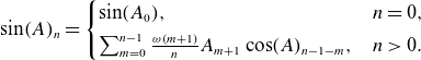 \begin{align} \sin (A)_n &= \begin{cases} \sin (A_0), & n = 0, \\[3pt] \sum _{m=0}^{n-1}\frac {\omega (m+1)}{n}A_{m+1}\cos (A)_{n-1-m}, & n \gt 0. \end{cases} \end{align}
B.5 Power
Now, we take a power $\alpha \neq 1$
of a series:
$\alpha \neq 1$
of a series:
 \begin{equation} B = A^{\alpha }. \end{equation}
Assuming $A_0 \neq 0$
, we have
$A_0 \neq 0$
, we have $B_0 = A_0^\alpha$
at leading order. At higher orders, we take the derivative with respect to
$B_0 = A_0^\alpha$
at leading order. At higher orders, we take the derivative with respect to $\rho$
to find
$\rho$
to find
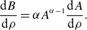 \begin{equation} \frac {\mathrm{d} B}{\mathrm{d} \rho } = \alpha A^{\alpha -1} \frac {\mathrm{d} A}{\mathrm{d} \rho }. \end{equation}
Multiplying both sides against $A$
, we find
$A$
, we find
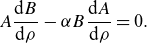 \begin{equation} A \frac {\mathrm{d} B}{\mathrm{d} \rho } - \alpha B \frac {\mathrm{d} A}{\mathrm{d} \rho } = 0. \end{equation}
Term by term, we have
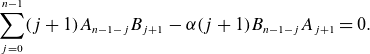 \begin{equation} \sum _{j = 0}^{n-1} (j+1) A_{n-1-j} B_{j+1} - \alpha (j+1) B_{n-1-j} A_{j+1} = 0. \end{equation}
This gives
 \begin{equation} B_{n} = \frac {1}{nA_0}\left (n \alpha A_n B_0 + \sum _{j=0}^{n-2} \big(j+1\big) \big(-A_{n-1-j} B_{j+1} + \alpha B_{n-1-j} A_{j+1}\big) \right )\!. \end{equation}
By substituting $j \to n-j-2$
, we reorder the right sum to find
$j \to n-j-2$
, we reorder the right sum to find
 \begin{equation} B_{n} = \frac {1}{nA_0}\left (n \alpha A_{n}B_0 + \sum _{j=0}^{n-2} \big(\alpha (n-j-1) - (j+1)\big) B_{j+1} A_{n-j-1} \right )\!. \end{equation}
B.6 Composition
Series composition is an important operation for changing coordinates. Consider that $A = A(x,y,s)$
, where
$A = A(x,y,s)$
, where $x=R \cos \Theta$
and
$x=R \cos \Theta$
and $y = R \sin \Theta$
. We would like to compose this with the functions
$y = R \sin \Theta$
. We would like to compose this with the functions $B(\rho ,\theta )$
and
$B(\rho ,\theta )$
and $C(\rho ,\theta )$
as
$C(\rho ,\theta )$
as $A(B,C,s)$
, where
$A(B,C,s)$
, where $B$
and
$B$
and $C$
replace the Cartesian cross-section coordinates
$C$
replace the Cartesian cross-section coordinates $x$
and
$x$
and $y$
. We note that this is preferable to composing with the polar coordinates
$y$
. We note that this is preferable to composing with the polar coordinates $R$
and
$R$
and $\Theta$
, as there are valid non-analytic transformations in these coordinates that keep
$\Theta$
, as there are valid non-analytic transformations in these coordinates that keep $A$
analytic. For this transformation, we assume that
$A$
analytic. For this transformation, we assume that $B_0 = C_0 = 0$
, i.e. there is no constant offset. We present the details for numerical Fourier series composition (4.1), but equivalent expressions could be used for other forms.
$B_0 = C_0 = 0$
, i.e. there is no constant offset. We present the details for numerical Fourier series composition (4.1), but equivalent expressions could be used for other forms.
The main observation we make for series composition is that if we can compute the basis functions
 \begin{equation} \Phi _{mn}(\rho ,\theta ,s) = R(\rho ,\theta ,s)^m \mathcal{F}_{2n-m}(\Theta (\rho ,\theta ,s)), \end{equation}
then the composition is simply
 \begin{equation} A(B,C,s) = \sum _{m=0}^{\infty } \sum _{n=0}^m A_{mn}(s) \Phi _{mn}(\rho ,\theta ,s), \end{equation}
where the multiplication in $s$
can be performed in spatial coordinates. So, the majority of the work is to find
$s$
can be performed in spatial coordinates. So, the majority of the work is to find $\Phi _{mn}$
, with the added perk that once the basis is found, further series compositions are faster.
$\Phi _{mn}$
, with the added perk that once the basis is found, further series compositions are faster.
To find the basis, we first notice that
 \begin{equation} \Phi _{00} = 1, \qquad \Phi _{10} = R\cos \Theta = C, \qquad \Phi _{11} = R\sin \Theta = B. \end{equation}
Then, further functions can be found by using angle-sum identities in the cosine case ( $m/2 \leqslant n \leqslant m+1$
)
$m/2 \leqslant n \leqslant m+1$
)
 \begin{align} \Phi _{m+1,n} &= R^{m+1}\cos ((2n-m-1)\Theta ),\nonumber \\ &= R^{m+1} \cos ((2(n-1)-m)\Theta )\cos (\Theta ) - R^{m+1} \sin ((2(n-1)-m)\Theta ) \sin (\Theta ),\nonumber \\ &= \Phi _{m,n-1} \Phi _{11} - \Phi _{m,m-n+1} \Phi _{10}, \end{align}
and the sine case ( $0\leqslant n\lt m/2$
)
$0\leqslant n\lt m/2$
)
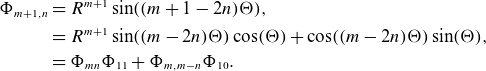 \begin{align} \Phi _{m+1,n} &= R^{m+1}\sin ((m + 1 - 2n)\Theta ),\nonumber \\ &= R^{m+1}\sin ((m-2n)\Theta )\cos (\Theta ) + \cos ((m-2n)\Theta )\sin (\Theta ), \nonumber \\ &= \Phi _{mn}\Phi _{11} + \Phi _{m,m-n}\Phi _{10}. \end{align}
B.7 Series inversion
Consider that we know the (Cartesian) flux coordinates $(B^{(1)}(x,y,s),{}B^{(2)}(x,y,s)) = (X,Y) = (R \cos \Theta , R \sin \Theta )$
and we want to know how to represent a function
$(B^{(1)}(x,y,s),{}B^{(2)}(x,y,s)) = (X,Y) = (R \cos \Theta , R \sin \Theta )$
and we want to know how to represent a function $A(\rho ,\theta ,s)$
in terms of
$A(\rho ,\theta ,s)$
in terms of $R$
and
$R$
and $\Theta$
. For this, we would use the series composition step presented in the previous section, but we need to obtain
$\Theta$
. For this, we would use the series composition step presented in the previous section, but we need to obtain $\rho$
and
$\rho$
and $\theta$
in terms of
$\theta$
in terms of $R$
and
$R$
and $\Theta$
, i.e. we need
$\Theta$
, i.e. we need $(C^{(1)}(X,Y,s), C^{(2)}(X,Y,s)) = (x,y) = (\rho \cos \theta , \rho \sin \theta )$
, where
$(C^{(1)}(X,Y,s), C^{(2)}(X,Y,s)) = (x,y) = (\rho \cos \theta , \rho \sin \theta )$
, where
 \begin{equation} \begin{pmatrix} C^{(1)}(B^{(1)},B^{(2)},s) \\ C^{(2)}(B^{(1)},B^{(2)},s) \end{pmatrix} = \begin{pmatrix} x \\ y \end{pmatrix}. \end{equation}
This is a step that is necessary if we have a series represented in direct coordinates, and we want to represent it in indirect (flux) coordinates.
We will solve this equation iteratively, assuming that we are using the real Fourier form (4.1). At leading order (assuming $C^{(i)}_0 = B^{(i)}_0 = 0$
), we have
$C^{(i)}_0 = B^{(i)}_0 = 0$
), we have
 \begin{equation} \left(\begin{array}{l@{\quad}l} C^{(1)}_{11} & C^{(1)}_{10} \\[2pt] C^{(2)}_{11} & C^{(2)}_{10} \end{array}\right) \left(\begin{array}{l@{\quad}l} B^{(1)}_{11} & B^{(1)}_{10} \\[2pt] B^{(2)}_{11} & B^{(2)}_{10} \end{array}\right) \begin{pmatrix} x \\ y \end{pmatrix} = \begin{pmatrix} x \\ y \end{pmatrix} \end{equation}
or
 \begin{equation} \left(\begin{array}{l@{\quad}l} C^{(1)}_{11} & C^{(1)}_{10} \\[2pt] C^{(2)}_{11} & C^{(2)}_{10} \end{array}\right) = \left(\begin{array}{l@{\quad}l} B^{(1)}_{11} & B^{(1)}_{10} \\[2pt] B^{(2)}_{11} & B^{(2)}_{10} \end{array}\right)^{-1}. \end{equation}
For the next orders, we note that we can compute $C^{(i)}_{\lt m+1}(B^{(1)}, B^{(2)}, s)$
using the composition formula, where we have chosen
$C^{(i)}_{\lt m+1}(B^{(1)}, B^{(2)}, s)$
using the composition formula, where we have chosen $C_{m}$
so this is identity up to order
$C_{m}$
so this is identity up to order $m+1$
. Substituting this into (B.32), we have
$m+1$
. Substituting this into (B.32), we have
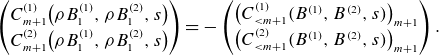 \begin{equation} \begin{pmatrix} C^{(1)}_{m+1}\big(\rho B^{(1)}_1, \rho B^{(2)}_1, s\big) \\[2pt] C^{(2)}_{m+1}\big(\rho B^{(1)}_1, \rho B^{(2)}_1, s\big) \end{pmatrix} = - \begin{pmatrix} \big(C^{(1)}_{\lt m+1}(B^{(1)}, B^{(2)}, s)\big)_{m+1} \\[2pt] \big(C^{(2)}_{\lt m+1}(B^{(1)}, B^{(2)}, s)\big)_{m+1} \end{pmatrix}. \end{equation}
If we build a basis $\Phi _{mn}$
from
$\Phi _{mn}$
from $B^{(i)}_1$
(see (B.27) and the following procedure) where
$B^{(i)}_1$
(see (B.27) and the following procedure) where
 \begin{equation} \Phi _{mn} = \sum _{k=0}^{\infty } \sum _{\ell =0}^k \Phi _{mnkl} \rho ^{k} \mathcal{F}_{k-2\ell }(\theta ), \end{equation}
the update can be expanded in index-notation as
 \begin{equation} \sum _{\ell =0}^{m+1} C^{(i)}_{m+1,\ell }\Phi _{m+1,\ell ,m+1,n} = -\big(C^{(1)}_{\lt m+1}(B^{(1)}, B^{(2)}, s)\big)_{m+1,n}. \end{equation}
Then, by inverting the matrix $\Psi _{\ell n} = \Phi _{m+1,\ell ,m+1,n}$
onto the right-hand side, we have the update for
$\Psi _{\ell n} = \Phi _{m+1,\ell ,m+1,n}$
onto the right-hand side, we have the update for $C^{(i)}_{m+1}$
.
$C^{(i)}_{m+1}$
.


 Open access