


1. Introduction
This paper is concerned with the suppression of oscillations in mixed convective flows in an open cavity permeated by a through-flow. It is inspired by the occurrence of such oscillations during the continuous casting of liquid metal alloys. In this type of process, solidified metal is pulled from the bottom of a pool of melted metal continuously fed from above. The pulling speed is adjusted to match that of the solidification front which, therefore, behaves as a steady but porous boundary for the fluid. A key issue is the appearance of oscillations resulting in unwanted macrosegregations (Dorward, Beerntsen & Brwon Reference Dorward, Beerntsen and Brwon1996; Beckermann Reference Beckermann, Buschow, Cahn, Flemings, Ilschner, Kramer, Mahajan and Veyssière2001) near the axis of the melt. We previously showed that the mechanism underpinning these oscillations could be reproduced in a simple hemispherical model of the sump (Flood & Davidson Reference Flood and Davidson1994) capturing the rather unusual interplay between the baroclinic convection caused by the cooled lateral wall (Pierrehumbert & Swanson Reference Pierrehumbert and Swanson1995) and the through-flow (Kumar & Pothérat Reference Kumar and Pothérat2020). Despite ignoring the complexities of the chemistry, multiple phase and solidification of the real process (Kuznetsov Reference Kuznetsov1997; Sheng & Jonsson Reference Sheng and Jonsson2000; Thomas & Zhang Reference Thomas and Zhang2001), the model produced three branches of linear instability: one supercritical and oscillatory; one subcritical and oscillatory; one supercritical and non-oscillatory when the Reynolds number $Re=u_0 H/\nu$
based on the inflow velocity
$Re=u_0 H/\nu$
based on the inflow velocity $u_0$
, sump height
$u_0$
, sump height $H$
and fluid kinematic viscosity
$H$
and fluid kinematic viscosity $\nu$
was varied. The topology of the oscillatory modes, consistent with observations in the casting process points to their hydrodynamic nature, and so validates the simplified hydrodynamic approach. The purpose of this paper is to take further advantage of the mathematical tractability of this model to design an actuation capable of suppressing these instabilities.
$\nu$
was varied. The topology of the oscillatory modes, consistent with observations in the casting process points to their hydrodynamic nature, and so validates the simplified hydrodynamic approach. The purpose of this paper is to take further advantage of the mathematical tractability of this model to design an actuation capable of suppressing these instabilities.
The idea of suppressing oscillations by means of an actuator producing oscillations at a well-chosen location has been long-exploited in thermoacoustics (Lieuwen Reference Lieuwen2003; Dowling & Morgans Reference Dowling and Morgans2005; Noiray et al. Reference Noiray, Durox, Schuller and Candel2009), in particular to control diffusion flames in combustion (Magri & Juniper Reference Magri and Juniper2013, Reference Magri and Juniper2014; Juniper & Sujith Reference Juniper and Sujith2018). However, it is yet to make its way to metallurgy, where oscillations occur on much larger time scales. Yet, both problems share similar challenges: the design of an effective control loop requires not only a sufficiently accurate model of the system’s dynamics but also sensors and actuators capable of feeding in the controller and enacting its output onto the process. The high temperatures, the highly corrosive nature of liquid metals and the risk of alloy contamination precludes the long-term immersion of any such device in the melt. Hence, just like in combustion problems, their implementation in hostile environments often proves impractical or unreliable (Mongia et al. Reference Mongia, Held, Hsiao and Pandalai2003), so in both cases, open-loop control using a single actuator is preferred for its simplicity and robustness. While these techniques have long been implemented in thermoacoustics with actuators placed within the flow (McManus, Vandsburger & Bowman Reference McManus, Vandsburger and Bowman1990; Lubarsky et al. Reference Lubarsky, Shcherbik, Bibik and Zinn2003), using them in liquid metals requires their positioning at the flow boundary. The key challenge is to find an actuation satisfying these conditions.
A possible solution lies in the idea of structural sensitivity, best voiced in the review of Luchini & Bottaro (Reference Luchini and Bottaro2014) on adjoint equations in stability problems. ‘The key reasoning is that, if indeed a specific spatially localised region (a wavemaker) acts as the driver of the oscillation and the rest of the flow just amplifies it, a structural perturbation acting in the amplifier portion is bound to affect only the amplitude (eigenvector) and not the frequency (eigenvalue) of the oscillation. Conversely, a perturbation in the wavemaker region mostly affects the eigenvalue. The structural sensitivity of the eigenvalue thus acts as a marker for the spatial location of the wavemaker’. For the problem we are considering structural sensitivity thus offers a method to calculate the position and topology of the actuation best suited to suppress the growth of the unstable mode underpinning the onset of oscillations. It is all the better suited as we already identified the unstable modes in a previous linear stability analysis (LSA) performed for each of the three branches appearing at different Reynolds numbers (Kumar & Pothérat Reference Kumar and Pothérat2020).
Indeed, structural sensitivity has successfully informed design alterations in devices where oscillations driven by instabilities took place, as in combustion problems or in the recent example of the stabilisation of inkjet in printers (Kungurtsev & Juniper Reference Kungurtsev and Juniper2019; Aguilar & Juniper Reference Aguilar and Juniper2020). The other common application of this approach concerns the a posteriori identification of suppression mechanisms where existing actuators are already implemented: the long misunderstood suppression of the von Kármán street by a small control cylinder placed in the near wake (Strykowski & Sreenivasan Reference Strykowski and Sreenivasan1990), was thus successfully explained when Marquet, Sipp & Jacquin (Reference Marquet, Sipp and Jacquin2008) were able to account for the feedback of the cylinder on both the unstable perturbation and the base flow. Further, a similar approach has been used in studying boundary-layer stability (Brandt et al. Reference Brandt, Marquet, Pralits and Sipp2011; Park & Zaki Reference Park and Zaki2019). Here we consider a different approach aligned with the industrial requirements of finding actuators best suited to suppress the oscillations and adaptable when the flow parameters are varied (here the Reynolds number, for example). Since such an actuator acts either mechanically or thermally on the system, we model this combined actuation by combining an external force in the momentum equations and an external source term in the energy equation. Since the adjoint mode corresponds to the Green function for the receptivity to an external actuation, aligning the forcing on it offers a way to directly control the amplitude of the unstable mode (see equation (3.10) from Giannetti & Luchini (Reference Giannetti and Luchini2007)). This approach follows a different principle from those based on base-flow sensitivity, as developed by Marquet et al. (Reference Marquet, Sipp and Jacquin2008). In these, the actuation aims to alter the base flow to shift the eigenvalue of the unstable mode towards the stable region. Hence, the idea is to shift the system so that it becomes stable. In our approach, by contrast, we do not alter the base flow or any other part of the base system but add an actuation that targets only the unstable mode once it grows. In the strategy using base-flow sensitivity, the actuation is optimised to alter the base flow, whereas in our receptivity-based strategy, the actuation must leave the base flow unaffected and act only on the perturbation. Doing so, however, raises three difficulties. First, we must ensure that the base flow is sufficiently unaffected by the actuation for the unstable mode to retain the topology targeted by the actuation. This can be verified using fully nonlinear simulations of the actuated system. Second, the linear theory does not provide an indication of the amplitude or the phase of the forcing, neither relative to that of the unstable mode, nor absolute. Both parameters therefore need to be varied to find the most effective combination for the suppression of the oscillations. Third, the system may evolve out of the linear regime where structural sensitivity operates. At this point, the system’s evolution ceases to follow that for which the forcing was designed in the first place. In control language, the system does not follow the controller’s model, so further applying the forcing may not result in the suppression predicted by the linear model. Hence the actuation may only be effective for a finite time. The question is whether this time is sufficiently long for any meaningful suppression strategy based on this approach.
We propose to answer these questions by performing the receptivity and sensitivity analyses (RSA) based on the stability analysis we conducted on the mixed convective flow in a cavity in Kumar & Pothérat (Reference Kumar and Pothérat2020) and numerically apply an external forcing built as described above. Besides exploring the idea of instability suppression by receptivity-informed external force, this problem carries three specificities of further fundamental interest from the physical and mathematical point of view. First, the mixed-convection character of this flow combines an open flow, for which structural sensitivity analysis has been perhaps most developed (Giannetti & Luchini Reference Giannetti and Luchini2007; Giannetti, Camarri & Luchini Reference Giannetti, Camarri and Luchini2010), with a buoyant flow, for which, to our knowledge, it was only used on stratified wakes (Chen & Spedding Reference Chen and Spedding2017). Aside of this example, open-loop control (Tang & Bau Reference Tang and Bau1998; Bau Reference Bau1999) and stabilisation by vibrating walls (Anilkumar et al. Reference Anilkumar, Grugel, Shen, Lee and Wang1993; Medelfef et al. Reference Medelfef, Henry, Kaddeche, Mokhtari, Bouarab, Botton and Bouabdallah2023) have been implemented in classical Rayleigh–Bénard and Marangoni flows. The adjoint equations for convective flows also made it possible to determine the influence of specific temperature distributions and heat fluxes at the flow boundaries (see Momose, Sasoh & Kimoto (Reference Momose, Sasoh and Kimoto1999) and others) and to infer past states of the Earth’s mantle (Bunge, Hagelberg & Travis Reference Bunge, Hagelberg and Travis2003; Ismail-Zadeh et al. Reference Ismail-Zadeh, Schubert, Tsepelev and Korotkii2004; Horbach, Bunge & Oeser Reference Horbach, Bunge and Oeser2014). Combining adjoint equations with LSA for the purpose of identifying the sources of convective instabilities and suppressing them, however, presents a new and interesting mathematical problem.
Convective flows are indeed particularly interesting in this context, as in most cases, they occur in combination with other effects such as shear flows in mixed convection (as in Vo, Pothérat & Sheard (Reference Vo, Pothérat and Sheard2017) and in the present case), or Lorentz and Coriolis forces in the vast field studying liquid planetary interiors (Roberts & King Reference Roberts and King2013). Because of this, the path to instability may follow different branches of instability, either individually near the onset or simultaneously in more supercritical regimes, leading to multimodality (Nakagawa Reference Nakagawa1957; Eltayeb Reference Eltayeb1972; Aujogue, Pothérat & Sreenivasan Reference Aujogue, Pothérat and Sreenivasan2015; Horn & Aurnou Reference Horn and Aurnou2022, 2024; Xu, Horn & Aurnou Reference Xu, Horn and Aurnou2023). For this reason, suppressing instabilities may require different actuations for different branches. These may even be used in combination in multimodal regimes, although their effectiveness may be limited if nonlinear interactions between these modes become significant. Whether the problem of mixed convection in a cavity may become multimodal when sufficiently supercritical is, at this point, an open question. For this reason, having in mind the aim of exploring the feasibility of suppressing convective oscillations using receptivity-informed actuation, we shall restrict ourselves to weakly supercritical regimes where instabilities are driven by a single unstable mode in each of the three branches of instability. This still leaves the question open as to whether the approach would be equally effective for each of them, especially so as these occur through bifurcations of different nature. Hence, we shall seek answers to the following questions.
-
(i) Does the system have significant receptivity in regions of the flow where an actuation can realistically be applied, in particular near the boundaries?
-
(ii) Which forcing parameters (phase and amplitude) are best suited for applying an external thermomechanical actuation, modelled on the adjoint of the eigenmode, to achieve suppression?
-
(iii) By how much can the energy of the oscillations be reduced and for how long?
-
(iv) Does an actuation purely based on linear dynamics remain effective when the nonlinearities are accounted for?
To answer these questions, we start by formulating the adjoint problem for mixed baroclinic convection in a nearly hemispherical cavity, as defined by Kumar & Pothérat (Reference Kumar and Pothérat2020) and recalled in § 2, along with a description of the numerical system based on high-order spectral elements methods. We then identify the thermomechanical source of the instabilities by performing RSA (§ 3). To determine the optimal phase and amplitude of the actuation based on the adjoint mode, relative to the unstable mode, we evolve the linearised equations, varying these values (§ 4). Finally, we put the idea to the test in fully nonlinear simulations and assess how long nonlinearities are kept at bay (§ 5).
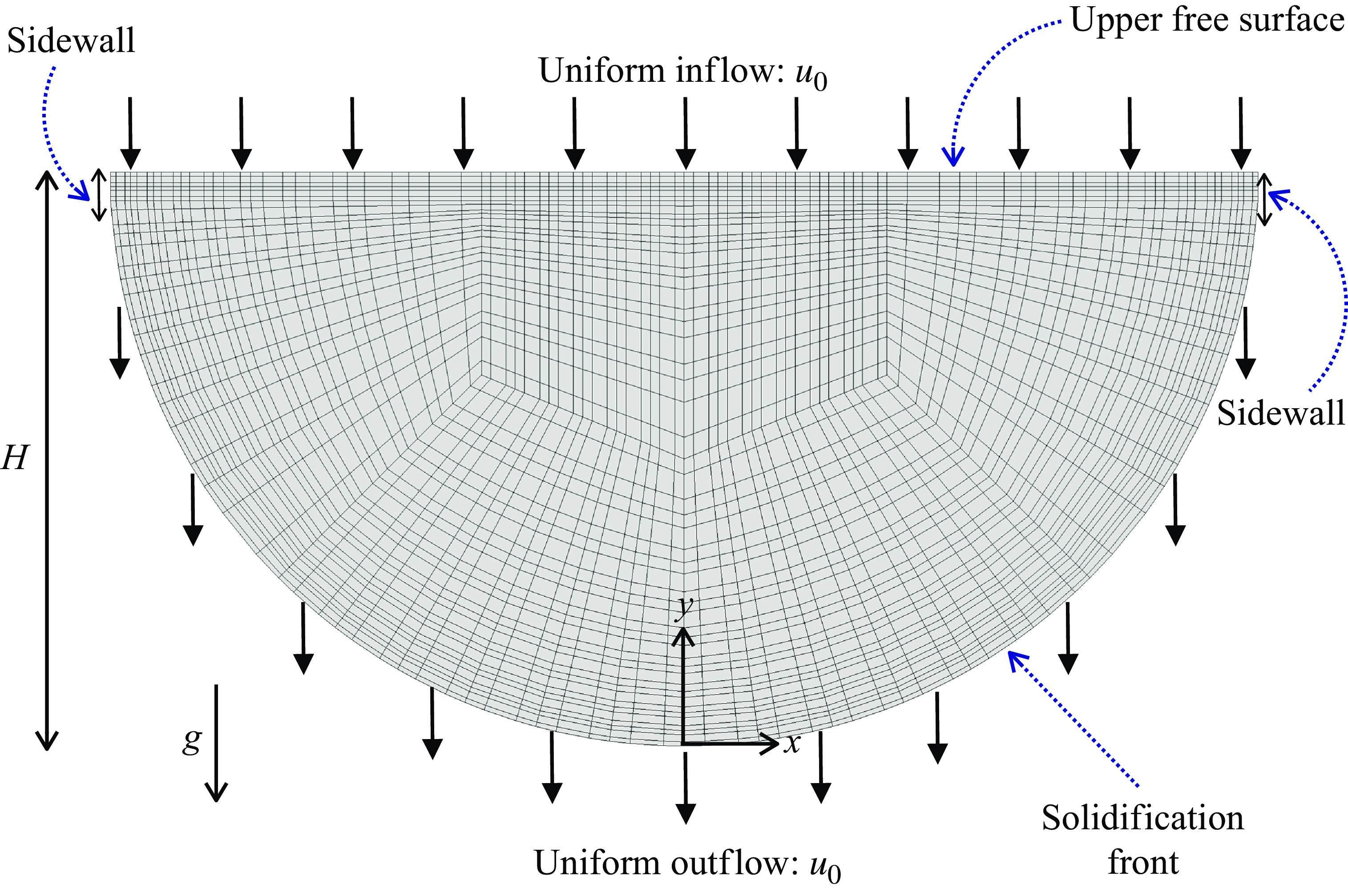
Problem geometry and mesh, with a rigid free surface at the inlet (top), solid side walls and a porous solid wall at the outlet (bottom, solidification front). The flow enters and leaves the domains at vertical velocity $u_0$
. The sketch also shows details of the mesh. This mesh consists of
$u_0$
. The sketch also shows details of the mesh. This mesh consists of $348$
quadrilateral elements, and each element is represented by the polynomial order of
$348$
quadrilateral elements, and each element is represented by the polynomial order of $N=3$
. Thus, the total collocation points are
$N=3$
. Thus, the total collocation points are $348 \times (N+1)^2 = 5568$
.
$348 \times (N+1)^2 = 5568$
.
2. Problem formulation
2.1. Governing equations
Following Kumar & Pothérat (Reference Kumar and Pothérat2020), we consider a cavity of height $H$
with an upper free surface where hot fluid is fed in, and a cold, porous lower boundary representing a solidification front, as shown in figure 1. The cavity is also assumed infinitely extended in the third direction (
$H$
with an upper free surface where hot fluid is fed in, and a cold, porous lower boundary representing a solidification front, as shown in figure 1. The cavity is also assumed infinitely extended in the third direction ( $\mathbf e_z$
). The lower boundary is semicircular and connected to the flat upper boundary by two solid, adiabatic side walls of height
$\mathbf e_z$
). The lower boundary is semicircular and connected to the flat upper boundary by two solid, adiabatic side walls of height $0.05H$
, with a temperature difference
$0.05H$
, with a temperature difference $\Delta T$
between the top and bottom boundaries. To model a liquid metal of density
$\Delta T$
between the top and bottom boundaries. To model a liquid metal of density $\rho$
, kinematic viscosity
$\rho$
, kinematic viscosity $\nu$
, thermal diffusivity
$\nu$
, thermal diffusivity $\alpha$
, thermal expansion coefficient
$\alpha$
, thermal expansion coefficient $\beta$
, the flow is assumed Newtonian and since temperature gradients remain moderate, its motion is assumed well described by the Oberbeck–Boussinesq approximation (Oberbeck Reference Oberbeck1879; Boussinesq Reference Boussinesq1903; Chandrasekhar Reference Chandrasekhar1961). This leads to the following non-dimensional governing equations:
$\beta$
, the flow is assumed Newtonian and since temperature gradients remain moderate, its motion is assumed well described by the Oberbeck–Boussinesq approximation (Oberbeck Reference Oberbeck1879; Boussinesq Reference Boussinesq1903; Chandrasekhar Reference Chandrasekhar1961). This leads to the following non-dimensional governing equations:
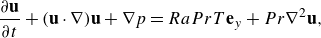 \begin{align} \frac {\partial \textbf{u}}{\partial t}+ (\textbf{u} \cdot \nabla) \textbf{u} + \nabla p & = RaPr T \textbf{e}_y+Pr \nabla ^2 \textbf{u}, \\[-12pt] \nonumber \end{align}
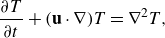 \begin{align} \frac {\partial T}{\partial t}+ (\textbf{u} \cdot \nabla) {T} & = \nabla ^2 T, \\[-12pt] \nonumber \end{align}
 \begin{align} \nabla \cdot \textbf{u} & = 0, \\[6pt] \nonumber \end{align}
where $\textbf{u}=(u,v,w)$
is the velocity vector field,
$\textbf{u}=(u,v,w)$
is the velocity vector field, $T$
is the temperature field,
$T$
is the temperature field, $t$
is the time and
$t$
is the time and $\mathbf g=-g\mathbf e_y$
is the gravitational acceleration. The modified pressure
$\mathbf g=-g\mathbf e_y$
is the gravitational acceleration. The modified pressure $p$
includes the buoyancy term that accounts for the reference temperature
$p$
includes the buoyancy term that accounts for the reference temperature $T_0$
at density
$T_0$
at density $\rho _0$
(Chandrasekhar Reference Chandrasekhar1961; Tritton Reference Tritton1988). The above set of equations are non-dimensionalised using length
$\rho _0$
(Chandrasekhar Reference Chandrasekhar1961; Tritton Reference Tritton1988). The above set of equations are non-dimensionalised using length $H$
, velocity
$H$
, velocity $\alpha /H$
, time
$\alpha /H$
, time $H^2/\alpha$
, pressure
$H^2/\alpha$
, pressure $\rho _0(\alpha /H)^2$
and temperature
$\rho _0(\alpha /H)^2$
and temperature $\Delta T$
. The equations feature two governing non-dimensional groups: the Prandtl number
$\Delta T$
. The equations feature two governing non-dimensional groups: the Prandtl number
 \begin{equation} Pr = \frac {\nu }{\alpha }, \end{equation}
which we fixed to $0.02$
, a typical value of aluminium alloys, and the Rayleigh number
$0.02$
, a typical value of aluminium alloys, and the Rayleigh number $Ra$
, defined as
$Ra$
, defined as
 \begin{equation} Ra = \frac {\beta g \Delta T H^3}{\nu \alpha }, \end{equation}
which controls the intensity of buoyancy forces relative to viscous forces. A free-slip boundary condition is applied to the upper boundary at $y=1$
with fluid being poured homogeneously across the boundary at an imposed temperature
$y=1$
with fluid being poured homogeneously across the boundary at an imposed temperature $\Delta T$
. These boundary conditions are expressed as
$\Delta T$
. These boundary conditions are expressed as
 \begin{eqnarray} \frac {\partial }{\partial y} \mathbf u\times \mathbf e_y=0, \qquad \mathbf u\cdot \mathbf e_y=RePr, \qquad T(y=1)=1, \end{eqnarray}
where $Re$
is the mass flux Reynolds number based on the dimensional feeding velocity
$Re$
is the mass flux Reynolds number based on the dimensional feeding velocity $u_0$
:
$u_0$
:
 \begin{equation} Re = \frac {u_0H}{\nu }. \end{equation}
At the lower boundary $\mathcal S$
, the solidification front is represented by solid, porous boundary conditions,
$\mathcal S$
, the solidification front is represented by solid, porous boundary conditions,
 \begin{eqnarray} \mathbf u_{\mathcal{S}}\times \mathbf e_y=0, \qquad \mathbf u_{\mathcal{S}}\cdot \mathbf e_y=RePr, \qquad T_{\mathcal{S}}=0, \end{eqnarray}
such that the flux of fluid pulled at $\mathcal{S}$
exactly cancels the flux of mass coming from the inlet. Impermeable, no-slip boundary conditions for the velocity field and insulating boundary conditions for the temperature field are imposed at the side walls (see figure 1). These boundary conditions for the temperature field at these side walls ensure that the temperature field remains continuous along the entire periphery of the domain. The pressure field in our calculation is obtained by solving the Poisson equation derived by taking the divergence of (2.1). A consistent Neumann boundary condition for pressure (Karniadakis & Israeli Reference Karniadakis, Israeli and Orszag1991) is applied at
$\mathcal{S}$
exactly cancels the flux of mass coming from the inlet. Impermeable, no-slip boundary conditions for the velocity field and insulating boundary conditions for the temperature field are imposed at the side walls (see figure 1). These boundary conditions for the temperature field at these side walls ensure that the temperature field remains continuous along the entire periphery of the domain. The pressure field in our calculation is obtained by solving the Poisson equation derived by taking the divergence of (2.1). A consistent Neumann boundary condition for pressure (Karniadakis & Israeli Reference Karniadakis, Israeli and Orszag1991) is applied at $y = 1$
, on the lower boundary
$y = 1$
, on the lower boundary $\mathcal{S}$
, and on the side walls. In the third direction
$\mathcal{S}$
, and on the side walls. In the third direction $\textbf{e}_z$
, the domain’s infinite extension is represented by periodic boundary conditions for all flow fields.
$\textbf{e}_z$
, the domain’s infinite extension is represented by periodic boundary conditions for all flow fields.
2.2. Direct and adjoint perturbation equations
The purpose of this work is to suppress linear instabilities with an actuation specifically designed to stifle the growth of linear perturbations. Since this actuation will be based on the linear dynamics of this perturbation, we first need the establish the set of equations that govern its linear dynamics. From Kumar & Pothérat (Reference Kumar and Pothérat2020), linear perturbations grow from a class of equilibrium solutions of (2.1)–(2.3) and boundary conditions (2.6) and (2.8) that are planar and invariant along $\textbf{e}_z$
, hence of the form
$\textbf{e}_z$
, hence of the form $\textbf{U}(x,y)$
,
$\textbf{U}(x,y)$
, $\bar {T}(x,y)$
. Baroclinicity due to the isothermal condition along the solidification front precludes any purely diffusive thermal equilibrium, so
$\bar {T}(x,y)$
. Baroclinicity due to the isothermal condition along the solidification front precludes any purely diffusive thermal equilibrium, so $\textbf{U}(x,y)$
is never homogeneously zero and both
$\textbf{U}(x,y)$
is never homogeneously zero and both $\textbf{U}(x,y)$
and
$\textbf{U}(x,y)$
and $\bar {T}(x,y)$
must be found as a fully nonlinear two-dimensional (2-D) solution of the equations. It follows that perturbations to this equilibrium
$\bar {T}(x,y)$
must be found as a fully nonlinear two-dimensional (2-D) solution of the equations. It follows that perturbations to this equilibrium $\textbf{q}^\prime (x,y,z,t)=(\textbf{u},T)^\top - (\textbf{U}, \bar {T})^\top =(\textbf{u}^\prime (x,y,z,t), T^\prime (x,y,z,t))^\top$
, are governed by the linear system of equations governing the evolution of infinitesimal perturbations,
$\textbf{q}^\prime (x,y,z,t)=(\textbf{u},T)^\top - (\textbf{U}, \bar {T})^\top =(\textbf{u}^\prime (x,y,z,t), T^\prime (x,y,z,t))^\top$
, are governed by the linear system of equations governing the evolution of infinitesimal perturbations,
 \begin{equation} \frac {\partial \textbf{q}^\prime }{\partial t} = \mathcal{L} \textbf{q}^\prime, \end{equation}
where
 \begin{equation} \mathcal{L}\textbf{q}^\prime = \begin{pmatrix} - (\textbf {U} \cdot \nabla) \textbf {u}^\prime -( \nabla \textbf{U}) \cdot \textbf {u}^\prime -\nabla p^\prime + RaPrT^\prime \textbf{e}_y+Pr{\nabla }^2\textbf{u}^\prime \\ -\textbf{U} \cdot \nabla T^\prime - (\nabla \bar {T})\cdot \textbf{u}^\prime + \nabla ^2 T^\prime \\ \end{pmatrix}. \end{equation}
Since $p^\prime$
is determined by the constraint
$p^\prime$
is determined by the constraint $\nabla \cdot \textbf{u}^\prime = 0$
, it is therefore not included in the state vector
$\nabla \cdot \textbf{u}^\prime = 0$
, it is therefore not included in the state vector $\textbf{q}^\prime$
. We will refer to (2.9) as the direct perturbation equation, and to
$\textbf{q}^\prime$
. We will refer to (2.9) as the direct perturbation equation, and to $\mathcal{L}$
as the direct linear operator. The boundary conditions for the base flow are the same as those for the main variables. As a result, the perturbation variables satisfy the homogeneous counterparts of the boundary conditions associated with the base flow. Since the base flow is invariant along
$\mathcal{L}$
as the direct linear operator. The boundary conditions for the base flow are the same as those for the main variables. As a result, the perturbation variables satisfy the homogeneous counterparts of the boundary conditions associated with the base flow. Since the base flow is invariant along $\textbf{e}_z$
and
$\textbf{e}_z$
and $\mathcal{L}$
does not explicitly depend upon time, the perturbation can be written as a linear combination of normal modes of the form,
$\mathcal{L}$
does not explicitly depend upon time, the perturbation can be written as a linear combination of normal modes of the form,
 \begin{equation} \textbf {q}^\prime (x,y,z,t) = \hat {\textbf {q}}(x,y) e^{ikz + \lambda t}, \end{equation}
where $k$
is the wavenumber along the homogenous direction
$k$
is the wavenumber along the homogenous direction $\textbf{e}_z$
and
$\textbf{e}_z$
and $\lambda = \sigma \pm i\omega$
contains the growth rate,
$\lambda = \sigma \pm i\omega$
contains the growth rate, $\sigma$
and frequency
$\sigma$
and frequency $\omega$
. The growth rate, frequency and the wavenumber of the most dominant mode
$\omega$
. The growth rate, frequency and the wavenumber of the most dominant mode $\hat {\textbf {q}}(x,y)=(\hat {u}, \hat {v}, \hat {w}, \hat {T})^\top$
(also referred to as the direct mode) are found by solving the eigenvalue problem for
$\hat {\textbf {q}}(x,y)=(\hat {u}, \hat {v}, \hat {w}, \hat {T})^\top$
(also referred to as the direct mode) are found by solving the eigenvalue problem for $\lambda$
that result from (2.9) and (2.11). This is done numerically by means of a time-stepper method (Barkley, Blackburn & Sherwin Reference Barkley, Blackburn and Sherwin2008). Here the eigenmodes are normalised such that
$\lambda$
that result from (2.9) and (2.11). This is done numerically by means of a time-stepper method (Barkley, Blackburn & Sherwin Reference Barkley, Blackburn and Sherwin2008). Here the eigenmodes are normalised such that $\|\hat {\textbf{q}}\|_2=1$
, where
$\|\hat {\textbf{q}}\|_2=1$
, where $\|\cdot \|_2$
denotes the standard
$\|\cdot \|_2$
denotes the standard $l^2$
vector norm of
$l^2$
vector norm of $4 \times N_e \times (N+1)^2$
values that make up
$4 \times N_e \times (N+1)^2$
values that make up $\hat {\textbf {q}}$
. In this context,
$\hat {\textbf {q}}$
. In this context, $N_e$
refers to the number of quadrilateral elements. For the details of the eigenvalue solver we refer the reader to § 2.2 of our previous work (Kumar & Pothérat Reference Kumar and Pothérat2020).
$N_e$
refers to the number of quadrilateral elements. For the details of the eigenvalue solver we refer the reader to § 2.2 of our previous work (Kumar & Pothérat Reference Kumar and Pothérat2020).
Next, we need to work out the form of the actuation that is best suited to suppress the growth of individual normal modes. The idea we pursue relies on the ideas of Giannetti & Luchini (Reference Giannetti and Luchini2007), who showed that the receptive regions of the direct linear modes are mapped by the adjoint eigenmodes of the same linearised equations. We, therefore, need to construct the adjoint operator $\mathcal{L}^*$
with respect to the time-averaged inner product relevant to the problem (Mao, Blackburn & Sherwin Reference Mao, Blackburn and Sherwin2015),
$\mathcal{L}^*$
with respect to the time-averaged inner product relevant to the problem (Mao, Blackburn & Sherwin Reference Mao, Blackburn and Sherwin2015),
 \begin{equation} (\textbf{a}, \textbf{b}) = \int _\Omega \textbf{a}\cdot \textbf{b} \, \text{d}V, \qquad \langle \textbf{c},\textbf{d} \rangle = \int _0^\tau (\textbf{c}, \textbf{d}) \, \textrm{d}t, \end{equation}
where $\textbf{a}$
and
$\textbf{a}$
and $\textbf{b}$
are time-averaged vector fields defined on the fluid domain
$\textbf{b}$
are time-averaged vector fields defined on the fluid domain $\Omega$
, while
$\Omega$
, while $\textbf{c}$
and
$\textbf{c}$
and $\textbf{d}$
are time-dependent vector fields defined on
$\textbf{d}$
are time-dependent vector fields defined on $\Omega$
and time domain
$\Omega$
and time domain $[0, \tau]$
. The adjoint operator is then defined by the relation
$[0, \tau]$
. The adjoint operator is then defined by the relation
 \begin{equation} \langle \textbf{q}^*, (-\partial _t +\mathcal{L})\textbf{q}^\prime \rangle - \langle (\partial _t+ \mathcal{L}^*)\textbf{q}^*, \textbf{q}^\prime \rangle =0, \end{equation}
and thus satisfies
 \begin{equation} -\frac {\partial \textbf{q}^*}{\partial t} = \mathcal{L}^* \textbf{q}^*, \end{equation}
where $\textbf{q}^*(x,y,z,t) = (u^*, v^*, w^*, T^*)^\top$
represents adjoint variables. The expression of
$\textbf{q}^*(x,y,z,t) = (u^*, v^*, w^*, T^*)^\top$
represents adjoint variables. The expression of $\mathcal L^*$
is readily derived by applying integration by parts to the first term in (2.13),
$\mathcal L^*$
is readily derived by applying integration by parts to the first term in (2.13),
 \begin{equation} \mathcal{L}^*\textbf{q}^* = \begin{pmatrix} (\textbf{U} \cdot \nabla) \mathbf{ u^*} - (\nabla \textbf{U})^\top \cdot \mathbf{ u^*} -(\nabla \bar {T})T^* -\nabla p^* + Pr{\nabla }^2\textbf{u}^* \\ (\textbf{U} \cdot \nabla) {T^*}+ RaPr\, v^*+\nabla ^2{T}^* \\ \end{pmatrix}, \end{equation}
with $\nabla \cdot \textbf{u}^* = 0$
. Similarly, the adjoint variables satisfy adjoint boundary conditions imposed by (2.13). These are identical to the boundary conditions satisfied by the direct variables, except for the
$\nabla \cdot \textbf{u}^* = 0$
. Similarly, the adjoint variables satisfy adjoint boundary conditions imposed by (2.13). These are identical to the boundary conditions satisfied by the direct variables, except for the $\textbf{e}_x$
and
$\textbf{e}_x$
and $\textbf{e}_z$
components of the velocity field at the upper free surface, that must satisfy Robin conditions (Barkley et al. Reference Barkley, Blackburn and Sherwin2008)
$\textbf{e}_z$
components of the velocity field at the upper free surface, that must satisfy Robin conditions (Barkley et al. Reference Barkley, Blackburn and Sherwin2008)
 \begin{equation} \textbf{e}_y \cdot \nabla u^* - Re \, u^*=0, \qquad \textbf{e}_y \cdot \nabla w^* -Re \, w^*=0. \end{equation}
Like the direct variables, the adjoint variables are decomposed into the normal modes but obtained as the solution of the adjoint eigenvalue problem, instead of the direct one so this time, the same eigenvalue solver yields the adjoint mode $\hat {\textbf {q}}^*(x,y)=(\hat {u}^*, \hat {v}^*, \hat {w}^*, \hat {T}^*)^\top$
. It follows from the biorthogonality property that the eigenvalue of the adjoint mode is the complex conjugate of that of the direct mode (Salwen & Grosch Reference Salwen and Grosch1981). Therefore, the magnitude of the growth rate and frequency of the adjoint and direct modes are identical when the real and imaginary parts of the complex eigenvalue are equated.
$\hat {\textbf {q}}^*(x,y)=(\hat {u}^*, \hat {v}^*, \hat {w}^*, \hat {T}^*)^\top$
. It follows from the biorthogonality property that the eigenvalue of the adjoint mode is the complex conjugate of that of the direct mode (Salwen & Grosch Reference Salwen and Grosch1981). Therefore, the magnitude of the growth rate and frequency of the adjoint and direct modes are identical when the real and imaginary parts of the complex eigenvalue are equated.
2.3. Receptivity and sensitivity
Giannetti & Luchini (Reference Giannetti and Luchini2007) showed that the adjoint field represented Green’s function for the receptivity problem. Therefore, the adjoint equations can be used to evaluate the effects of any external actuation or a generic initial condition on the leading eigenmode of the direct problem (2.9). This property forms the basis for the analysis in § 4, where we seek to identify the regions where applying an actuation would most effectively affect the growth of unstable modes. Our intention is to control the growth of the perturbation from an initial condition where the unstable mode has already grown measurably, but sufficiently little to remain within the confines of the linear approximation. For this purpose, we determine the topology of the actuation on the adjoint eigenmode. A common alternative approach is to force the system in such a way as to modify the underlying operator such that the eigenvalue associated with the leading eigenmode remains in the stable region, ignoring the initial condition. The optimal actuation for this purpose is given by the sensitivity map. The relative shift in the eigenvalue, and therefore the growth rate associated with the direct and the adjoint mode incurred by acting at any given location of the flow is given by the sensitivity map (Giannetti & Luchini Reference Giannetti and Luchini2007; Giannetti et al. Reference Giannetti, Camarri and Luchini2010; Qadri, Mistry & Juniper Reference Qadri, Mistry and Juniper2013)
 \begin{equation} S_{ij}(x,y)=\frac {\hat {\textbf {q}}_i \hat {\textbf {q}}^*_j }{\int _\Omega \hat {\textbf {q}}^\top \hat {\textbf {q}}^* \, \text{d}x\text{d}y}.\end{equation}
Note that the sensitivity tensor above is based on feedback localised in space, of the form ${\mathbf C_0} \delta ({\mathbf x} - {\mathbf x_0}) \hat {\textbf {q}}$
. Here,
${\mathbf C_0} \delta ({\mathbf x} - {\mathbf x_0}) \hat {\textbf {q}}$
. Here, $\mathbf C_0$
denotes a constant coefficient matrix,
$\mathbf C_0$
denotes a constant coefficient matrix, $\mathbf x_0$
indicates the position where the feedback acts and
$\mathbf x_0$
indicates the position where the feedback acts and $\delta ({\mathbf x} - {\mathbf x_0})$
denotes the Dirac delta function. Tensor
$\delta ({\mathbf x} - {\mathbf x_0})$
denotes the Dirac delta function. Tensor $S_{ij}$
determines the relative local intensity of the feedback of individual component
$S_{ij}$
determines the relative local intensity of the feedback of individual component $\hat {\textbf {q}}^*_j$
onto the individual component
$\hat {\textbf {q}}^*_j$
onto the individual component $\hat {\textbf {q}}_i$
of the eigenmode. This quantity also locates the regions of the flow acting as wavemakers. In particular, since
$\hat {\textbf {q}}_i$
of the eigenmode. This quantity also locates the regions of the flow acting as wavemakers. In particular, since ${\mathbf q}^\prime$
and
${\mathbf q}^\prime$
and $\mathbf q^*$
contain all three components of velocity and the temperature, the knowledge of
$\mathbf q^*$
contain all three components of velocity and the temperature, the knowledge of $S_{ij}$
indicates whether the actuation should be of a thermal or mechanical nature and if mechanical, which component of the velocity (or combination of all four components including temperature) is most efficient at altering the growth of the unstable mode. Both the direct and adjoint problems being linear, amplitudes are relative so we may further normalise the direct and adjoint modes by choosing (Giannetti & Luchini Reference Giannetti and Luchini2007)
$S_{ij}$
indicates whether the actuation should be of a thermal or mechanical nature and if mechanical, which component of the velocity (or combination of all four components including temperature) is most efficient at altering the growth of the unstable mode. Both the direct and adjoint problems being linear, amplitudes are relative so we may further normalise the direct and adjoint modes by choosing (Giannetti & Luchini Reference Giannetti and Luchini2007)
 \begin{equation} \int _\Omega \hat {\textbf {q}}^\top \hat {\textbf {q}}^* \, \text{d}x\text{d}y = 1, \end{equation}
so that the sensitivity tensor is simply expressed as $S_{ij}=\hat {\textbf {q}}_i \hat {\textbf {q}}^*_j$
.
$S_{ij}=\hat {\textbf {q}}_i \hat {\textbf {q}}^*_j$
.
At this point, we reiterate that our study considers the feedback on the perturbed field. This differs from the approach of Marquet et al. (Reference Marquet, Sipp and Jacquin2008), which examines the effect of forcing on the base flow. The objective of our study is to apply a forcing based on the adjoint mode (receptivity) to suppress instability. In general, the forcing influences both the base flow and the perturbation and this effect can be analysed in detail by studying the sensitivity to base flow modification as Marquet et al. (Reference Marquet, Sipp and Jacquin2008) do or by validating the approach using nonlinear direct numerical simulation (DNS) as we do in this paper. To summarise the difference between these two strategies in a nutshell, our strategy consists in applying a forcing that suppresses the instability before either the perturbation or the forcing has sufficiently grown to affect the base flow. The strategy proposed by Marquet et al. (Reference Marquet, Sipp and Jacquin2008), by contrast, is to modify the base flow to prevent the perturbation from growing at all.
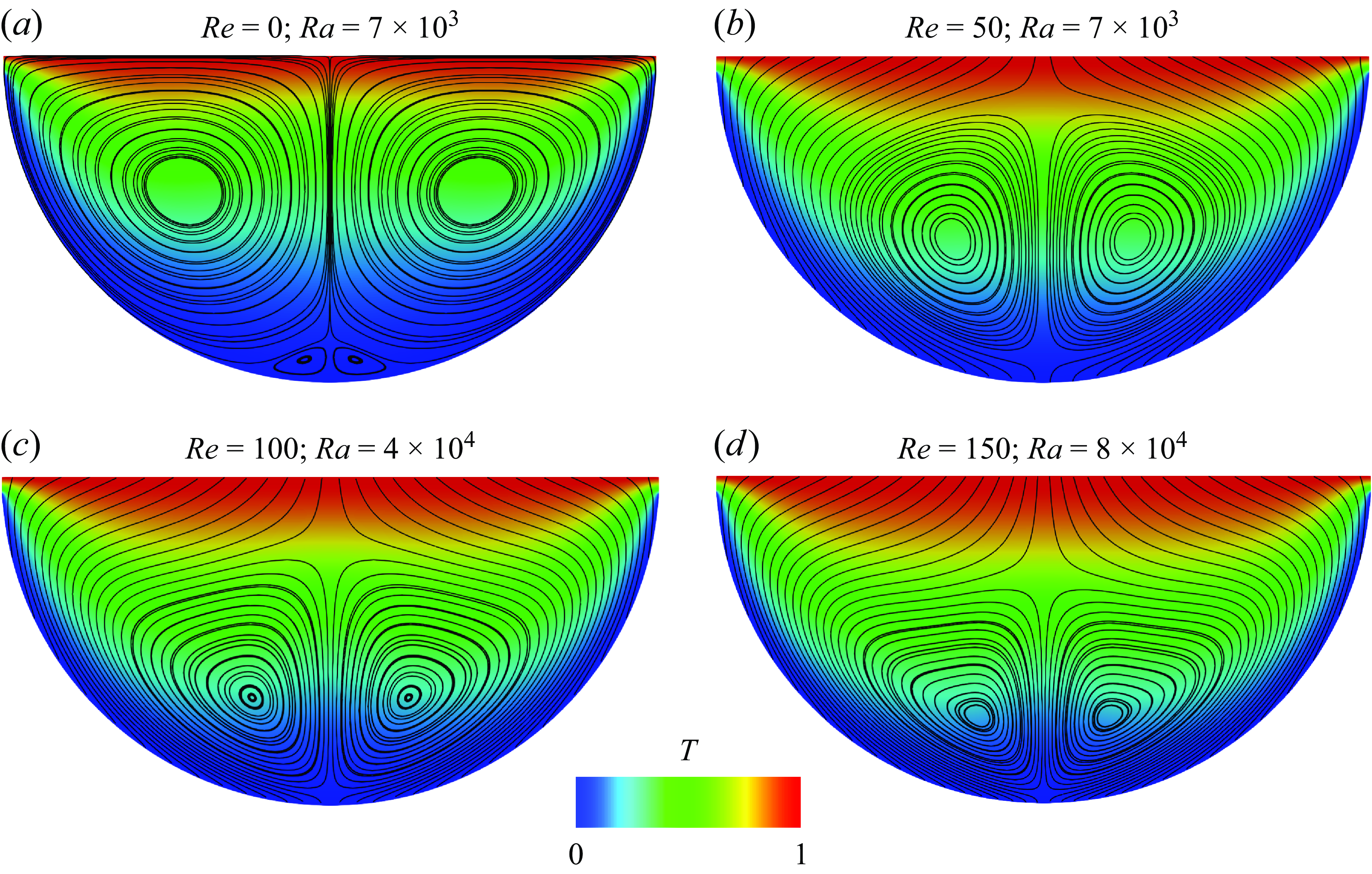
Streamlines of the steady 2-D base flow and temperature field for the simulation cases (a) C1, (b) C2, (c) C3 and (d) C4.
2.4. Methodology and choice of parameters
For the reminder of the paper, we shall proceed as follows to find and assess the actuation best suited to damp the growth of linear instabilities. First, the steady 2-D base flow solutions are obtained using DNS of (2.1)–(2.3) together with the associated boundary conditions. Second, the LSA of the 2-D base flow against three-dimensional (3-D) perturbations is carried out by solving the eigenvalue problem for operator $\mathcal L$
. These first two steps were previously carried out over an extensive range of governing parameters and wavenumbers
$\mathcal L$
. These first two steps were previously carried out over an extensive range of governing parameters and wavenumbers $k$
in Kumar & Pothérat (Reference Kumar and Pothérat2020). Here, we repeat the same approach for flows that are weakly supercritical so as to focus on cases where the instability is driven by a small number of unstable modes. The idea behind this strategy is that even in the fully nonlinear evolution, if the instability remains driven by a small-enough number of modes, it may be enough to prevent the growth of the most unstable of them to stop the growth of instabilities altogether. This approach is not expected to be successful if the base flow is destabilised by a broad spectrum of fast-growing unstable modes, as may be the case in more strongly supercritical cases. On this basis, we select four typical weakly supercritical cases illustrating the different instability mechanisms identified in this previous work.
$k$
in Kumar & Pothérat (Reference Kumar and Pothérat2020). Here, we repeat the same approach for flows that are weakly supercritical so as to focus on cases where the instability is driven by a small number of unstable modes. The idea behind this strategy is that even in the fully nonlinear evolution, if the instability remains driven by a small-enough number of modes, it may be enough to prevent the growth of the most unstable of them to stop the growth of instabilities altogether. This approach is not expected to be successful if the base flow is destabilised by a broad spectrum of fast-growing unstable modes, as may be the case in more strongly supercritical cases. On this basis, we select four typical weakly supercritical cases illustrating the different instability mechanisms identified in this previous work.
-
(i) Simulation case C1 ( $Re = 0; Ra=7 \times 10^3$
). This case corresponds to a purely convective base flow with zero inlet (and outlet) mass flux, i.e. no fluid crosses the boundaries of the flow domain (see figure 2
a). The flow becomes unstable to a travelling wave at
$Ra_c=5.975 \times 10^3$
, through a supercritical Hopf bifurcation. The corresponding branch in the complex eigenmode spectrum is labelled type II.
$Re = 0; Ra=7 \times 10^3$
). This case corresponds to a purely convective base flow with zero inlet (and outlet) mass flux, i.e. no fluid crosses the boundaries of the flow domain (see figure 2
a). The flow becomes unstable to a travelling wave at
$Ra_c=5.975 \times 10^3$
, through a supercritical Hopf bifurcation. The corresponding branch in the complex eigenmode spectrum is labelled type II. -
(ii) Simulation case C2 (
$Re = 50; Ra=7 \times 10^3$
). This case features an inflow through the upper boundary as shown in figure 2(b). The flow becomes unstable to a type II travelling wave through a supercritical Hopf bifurcation. -
(iii) Simulation case C3 (
$Re = 100; Ra=4 \times 10^4$
). This case is similar to C2 but with more intense inflow. The base flow is presented in figure 2(c). At
$Ra_c=3.621 \times 10^4$
, it becomes unstable to a leading mode from a different branch (type I), that is still oscillatory but arises out of a subcritical Hopf bifurcation. -
(iv) Simulation case C4 (
$Re = 150; Ra=8 \times 10^4$
). Here the flow is mostly driven by the inflow (see figure 2
d). The instability corresponds to a further branch of the eigenvalue spectrum labelled type III and yields a non-oscillatory mode through a supercritical pitchfork bifurcation.


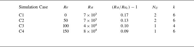
Details of the above selected parameters are tabulated in table 1.
Parameters of the weakly supercritical cases, C1, C2, C3 and C4, were selected for the analysis. Here $(Ra/Ra_c)-1$
represents the level of criticality, where
$(Ra/Ra_c)-1$
represents the level of criticality, where $Ra_c$
is the critical Rayleigh number;
$Ra_c$
is the critical Rayleigh number; $N_U$
represents the number of unstable modes;
$N_U$
represents the number of unstable modes; $k$
represents the most unstable mode. Note that
$k$
represents the most unstable mode. Note that $Ra_c$
for the each case is obtained from table 2 of Kumar & Pothérat (Reference Kumar and Pothérat2020).
$Ra_c$
for the each case is obtained from table 2 of Kumar & Pothérat (Reference Kumar and Pothérat2020).
Additionally to this previous analysis, we now need to calculate adjoint modes to perform the RSA. These are obtained by solving the eigenvalue problem for the operator $\mathcal{L}^*$
using the same method as for the LSA. Third, the evolution of the normal mode targeted for suppression is calculated using the linearised Navier–Stokes equations (2.9), to which a forcing term based on the adjoint eigenmode is added on the left-hand side. We use two types of actuation to that effect. As the unstable mode is suppressed by the forcing, its amplitude varies, and so does the amplitude of the actuation. Otherwise, once the unstable mode is suppressed, the actuation would act as an external force taking the flow away from its equilibrium. Hence, to assess the ability of an actuation based on the receptivity map to suppress the unstable mode, we use a forcing of the form
$\mathcal{L}^*$
using the same method as for the LSA. Third, the evolution of the normal mode targeted for suppression is calculated using the linearised Navier–Stokes equations (2.9), to which a forcing term based on the adjoint eigenmode is added on the left-hand side. We use two types of actuation to that effect. As the unstable mode is suppressed by the forcing, its amplitude varies, and so does the amplitude of the actuation. Otherwise, once the unstable mode is suppressed, the actuation would act as an external force taking the flow away from its equilibrium. Hence, to assess the ability of an actuation based on the receptivity map to suppress the unstable mode, we use a forcing of the form
 \begin{equation} \textbf{f}(x,y,z,t) = \alpha (t)\Re \{A\hat {\textbf {q}}^*(x,y)\exp {[ \sigma t + i(kz + \omega t + \phi)]}\}, \end{equation}
where $\alpha (t)$
represents the amplitude of the unstable mode normalised by its initial value. In practice, adapting the forcing to the amplitude in real time would require sensing and processing capable of extracting the evolution of the unstable mode instantaneously, which, in the harsh environment of continuous casting, is impractical. Instead, it is much easier to set a threshold on the sensor output above which an actuation of constant amplitude is applied. For this purpose, we use a simpler form of actuation,
$\alpha (t)$
represents the amplitude of the unstable mode normalised by its initial value. In practice, adapting the forcing to the amplitude in real time would require sensing and processing capable of extracting the evolution of the unstable mode instantaneously, which, in the harsh environment of continuous casting, is impractical. Instead, it is much easier to set a threshold on the sensor output above which an actuation of constant amplitude is applied. For this purpose, we use a simpler form of actuation,
 \begin{equation} \textbf{f}(x,y,z,t) = \Re \{A\hat {\textbf {q}}^*(x,y)\exp {[ \sigma t + i(kz + \omega t + \phi)]}\}. \end{equation}
In both cases, $A$
and
$A$
and $\phi$
represent the initial real amplitude and real phase of the forcing, respectively, relative to the unstable mode. Note that our strategy is not to choose an actuation intended to manipulate the eigenvalue associated with the leading eigenmode. This well-established technique entails applying a force whose linear dependence on the unstable eigenmode shifts the leading eigenvalue of the linear evolution operator to the stable region. The topology of the optimal forcing map is, in this case, provided by the structural sensitivity, or base-flow sensitivity maps (Giannetti & Luchini Reference Giannetti and Luchini2007; Marquet et al. Reference Marquet, Sipp and Jacquin2008). Instead, we chose to apply a predetermined force, i.e. that does not depend linearly on variable
$\phi$
represent the initial real amplitude and real phase of the forcing, respectively, relative to the unstable mode. Note that our strategy is not to choose an actuation intended to manipulate the eigenvalue associated with the leading eigenmode. This well-established technique entails applying a force whose linear dependence on the unstable eigenmode shifts the leading eigenvalue of the linear evolution operator to the stable region. The topology of the optimal forcing map is, in this case, provided by the structural sensitivity, or base-flow sensitivity maps (Giannetti & Luchini Reference Giannetti and Luchini2007; Marquet et al. Reference Marquet, Sipp and Jacquin2008). Instead, we chose to apply a predetermined force, i.e. that does not depend linearly on variable $\hat {\textbf {q}}$
. That actuation is designed to suppress the amplitude of the unstable mode from a small but finite initial value. Since the actuation does not linearly depend on
$\hat {\textbf {q}}$
. That actuation is designed to suppress the amplitude of the unstable mode from a small but finite initial value. Since the actuation does not linearly depend on $\hat {\textbf {q}}$
, the evolution equation is not strictly linear, its linear part does not change and neither does the leading eigenvalue. The actuation f has four components. The first three components represent mechanical forces, and the last component represents thermal forces. This step serves two purposes. First, it acts as a validation of the strategy. Since the forcing is derived from linearised adjoint equations, that ignore nonlinear interactions, it must at least be effective at damping the direct linear mode, to carry any hope of preventing the full nonlinear growth of the instability. Second, building the forcing on the topology of the adjoint mode involves a choice of amplitude and phase relative to the direct modes. To find out the optimal values of both, we carry out a series of linear simulations where they are varied.
$\hat {\textbf {q}}$
, the evolution equation is not strictly linear, its linear part does not change and neither does the leading eigenvalue. The actuation f has four components. The first three components represent mechanical forces, and the last component represents thermal forces. This step serves two purposes. First, it acts as a validation of the strategy. Since the forcing is derived from linearised adjoint equations, that ignore nonlinear interactions, it must at least be effective at damping the direct linear mode, to carry any hope of preventing the full nonlinear growth of the instability. Second, building the forcing on the topology of the adjoint mode involves a choice of amplitude and phase relative to the direct modes. To find out the optimal values of both, we carry out a series of linear simulations where they are varied.
Finally, with the knowledge of the optimal amplitude and phase of the actuation, we test the suppression of instability with its full nonlinear dynamics through 3-D DNS (the detail of individual simulations is given in § 5).
2.5. Numerical set-up
The methodology outlined in the previous section involves four types of numerical computations: 2-D (nonlinear) DNS; direct and adjoint eigenvalue problems; 3-D evolution of individual eigenmodes through the direct linearised equations; 3-D (nonlinear) DNS. The solution of the direct and adjoint eigenvalue problems are found by means of the time-stepping method implemented and tested in detail in Kumar & Pothérat (Reference Kumar and Pothérat2020). The novelty compared with this previous work is the solution of the adjoint eigenvalue problem, which was validated by making sure the eigenvalues obtained from both the LSA and RSA yielded the same results down to machine precision.
The nonlinear governing equations (2.1)–(2.3), the direct perturbation equation (2.9) and the adjoint equation (2.14) are solved using the spectral-element code Nektar++ (Cantwell et al. Reference Cantwell2015; Moxey et al. Reference Moxey2020). We adopted a spectral-element discretisation in the $x{-}y$
plane with a mesh consisting of 348 quadrilateral elements. For the 3-D simulations, we used a Fourier-based spectral method (Bolis et al. Reference Bolis, Cantwell, Moxey, Serson and Sherwin2016) for discretisation in the
$x{-}y$
plane with a mesh consisting of 348 quadrilateral elements. For the 3-D simulations, we used a Fourier-based spectral method (Bolis et al. Reference Bolis, Cantwell, Moxey, Serson and Sherwin2016) for discretisation in the $\textbf{e}_z$
direction. The computational domain extends along
$\textbf{e}_z$
direction. The computational domain extends along $\textbf{e}_z$
by
$\textbf{e}_z$
by $2\pi$
. A third-order implicit–explicit method (Vos et al. Reference Vos, Eskilsson, Bolis, Chun, Kirby and Sherwin2011) is used for time stepping. For all four types of numerical calculations, the time step
$2\pi$
. A third-order implicit–explicit method (Vos et al. Reference Vos, Eskilsson, Bolis, Chun, Kirby and Sherwin2011) is used for time stepping. For all four types of numerical calculations, the time step $\Delta t$
was kept constant so that the maximum local Courant number
$\Delta t$
was kept constant so that the maximum local Courant number $C_{max }$
remained below unity everywhere in the domain at all times. The numerical implementation is described and tested in detail in Kumar & Pothérat (Reference Kumar and Pothérat2020). Figure 1 shows the details of a 2-D
$C_{max }$
remained below unity everywhere in the domain at all times. The numerical implementation is described and tested in detail in Kumar & Pothérat (Reference Kumar and Pothérat2020). Figure 1 shows the details of a 2-D $x{-}y$
mesh generated using the Gmsh package (Geuzaine & Remacle Reference Geuzaine and Remacle2009) with polynomial order
$x{-}y$
mesh generated using the Gmsh package (Geuzaine & Remacle Reference Geuzaine and Remacle2009) with polynomial order $N = 3$
as an example of spatial–spectral discretisation used in the
$N = 3$
as an example of spatial–spectral discretisation used in the $(x,y)$
plane. Elements at the edges are more densely packed than in the bulk, with a ratio of four between the edge sizes of the largest and the smallest elements. On each element, the flow variables are projected onto the polynomial basis represented at Gauss–Lobatto–Legendre points. As in our previous work, we perform a convergence test on the polynomial order for the leading eigenvalue for each case to ensure the solution is independent of the spectral order. For example, the leading eigenvalue computed for the simulation case C4 with the polynomial order
$(x,y)$
plane. Elements at the edges are more densely packed than in the bulk, with a ratio of four between the edge sizes of the largest and the smallest elements. On each element, the flow variables are projected onto the polynomial basis represented at Gauss–Lobatto–Legendre points. As in our previous work, we perform a convergence test on the polynomial order for the leading eigenvalue for each case to ensure the solution is independent of the spectral order. For example, the leading eigenvalue computed for the simulation case C4 with the polynomial order $N=8$
differs by less than 0.04 % from the calculation performed with
$N=8$
differs by less than 0.04 % from the calculation performed with $N=9$
. Convergence of the leading eigenvalue with the polynomial order is presented in table 2. Similar convergence tests have been conducted for other simulation cases. For all 3-D DNS calculations, we have retained 32 Fourier modes along
$N=9$
. Convergence of the leading eigenvalue with the polynomial order is presented in table 2. Similar convergence tests have been conducted for other simulation cases. For all 3-D DNS calculations, we have retained 32 Fourier modes along $\textbf{e}_z$
, which are deemed adequate based on our previous convergence test conducted in Kumar & Pothérat (Reference Kumar and Pothérat2020).
$\textbf{e}_z$
, which are deemed adequate based on our previous convergence test conducted in Kumar & Pothérat (Reference Kumar and Pothérat2020).
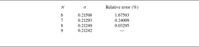
We examine the relationship between the leading eigenvalues and the polynomial order $N$
. The leading eigenvalues are computed on the mesh at
$N$
. The leading eigenvalues are computed on the mesh at $Re=150$
,
$Re=150$
, $Ra=8 \times 10^4$
and
$Ra=8 \times 10^4$
and $k=6$
. The relative error is calculated with respect to the case of the highest polynomial order (
$k=6$
. The relative error is calculated with respect to the case of the highest polynomial order ( $N=9$
).
$N=9$
).
3. Linear RSA
The aim of this section is to identify the most effective location within the flow domain for an actuation to suppress instabilities using RSA. The receptivity analysis returns a map of the physical locations within the flow domain where one can act on the instabilities by applying an external actuation. On the other hand, the sensitivity analysis identifies the location in the flow domain where this external actuation would incur the greatest flow alteration. For this purpose, we shall discuss each of the cases C1–C4 outlined in § 2.4.
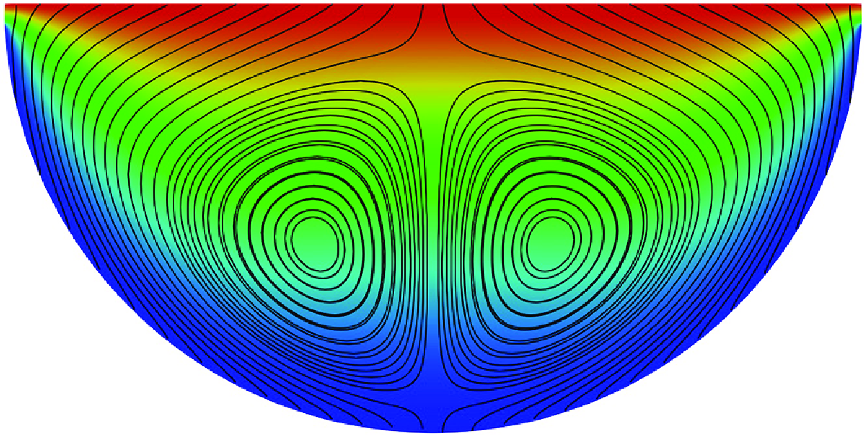
Spatial distribution of the velocity field modulus ( $\|\hat {\textbf {u}}\|$
), receptivity to momentum forcing (
$\|\hat {\textbf {u}}\|$
), receptivity to momentum forcing ( $\|\hat {\textbf {u}}^*\|$
) and the Frobenius norm of the momentum structural sensitivity (
$\|\hat {\textbf {u}}^*\|$
) and the Frobenius norm of the momentum structural sensitivity ( $\|\hat {\textbf {u}}\|\|\hat {\textbf {u}}^*\|$
) for the simulation cases: (a)–(c) C1; (d)–(f) C2; (g)–(i) C3; (j)-(l) C4. Panel (m) represents the zoomed region of
$\|\hat {\textbf {u}}\|\|\hat {\textbf {u}}^*\|$
) for the simulation cases: (a)–(c) C1; (d)–(f) C2; (g)–(i) C3; (j)-(l) C4. Panel (m) represents the zoomed region of $\|\hat {\textbf {u}}^*\|$
for C4. The streamlines in (a), (d), (g) and (j) represent the real part of the unstable eigenmode (
$\|\hat {\textbf {u}}^*\|$
for C4. The streamlines in (a), (d), (g) and (j) represent the real part of the unstable eigenmode ( $\Re ({\hat {u}})\textbf{e}_x + \Re ({\hat {v}})\textbf{e}_y$
) in the
$\Re ({\hat {u}})\textbf{e}_x + \Re ({\hat {v}})\textbf{e}_y$
) in the $x{-}y$
plane.
$x{-}y$
plane.
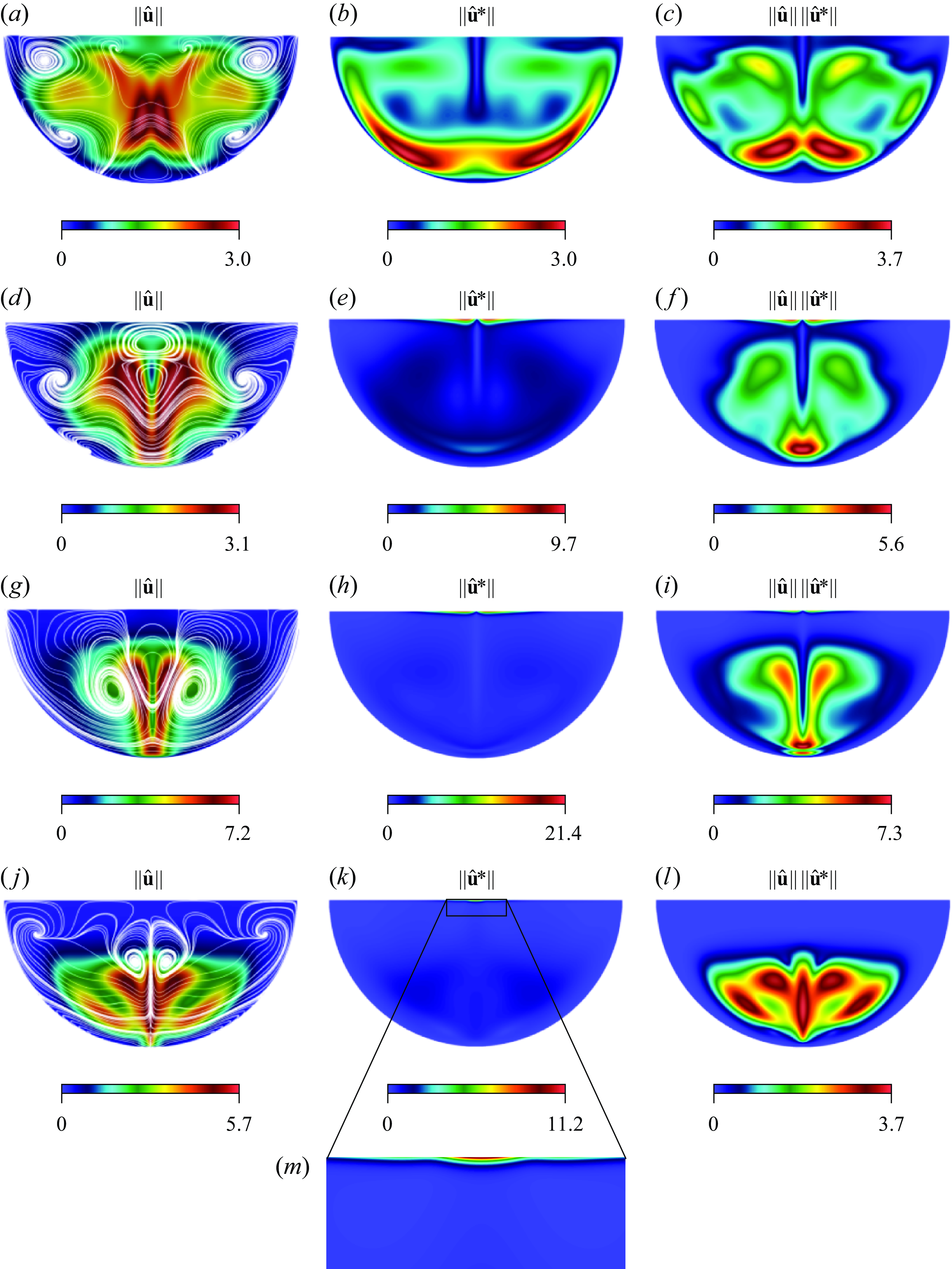
For case C1, the base flow, represented on figure 2(a), consists of two symmetric baroclinically driven recirculation cells driven along the solidification front, from the maximum baroclinicity regions in the upper left- and right-hand corners. Both cells meet on the axis near the bottom of the domain and drive a strong upward jet there. The leading unstable mode of type II (with critical parameters $k_c=6.3$
,
$k_c=6.3$
, $Ra_c = 5.975 \times 10^3$
) arises out of shear instability near the location of the maximum velocity along that jet (see figure 3
a). It consists of a wave travelling in the
$Ra_c = 5.975 \times 10^3$
) arises out of shear instability near the location of the maximum velocity along that jet (see figure 3
a). It consists of a wave travelling in the $z$
direction, and appears through a supercritical Hopf bifurcation.
$z$
direction, and appears through a supercritical Hopf bifurcation.
The velocity field modulus associated with the adjoint mode $\|\hat {\textbf {u}}^*\|$
, which represents receptivity, is displayed in figure 3(b). The most receptive region is located at the wall, where the magnitude of two jets is strongest. The product of direct and adjoint modes represents the sensitivity and is plotted in figure 3(c). This plot shows that the sensitivity is symmetric about the central axis, and strong towards the bottom of the cavity.
$\|\hat {\textbf {u}}^*\|$
, which represents receptivity, is displayed in figure 3(b). The most receptive region is located at the wall, where the magnitude of two jets is strongest. The product of direct and adjoint modes represents the sensitivity and is plotted in figure 3(c). This plot shows that the sensitivity is symmetric about the central axis, and strong towards the bottom of the cavity.
For case C2, the presence of the inflow through the top boundary opposes the upward jet seen in case C1 and therefore suppresses the baroclinically driven recirculation. These are displaced downwards as a result and the shear is less concentrated near the symmetry axis as represented in figure 2(b). Accordingly, the unstable mode ( $k_c=6.2$
,
$k_c=6.2$
, $Ra_c=6.168 \times 10^3$
, figure 3
d) is more widely spread along the two directions of space than in case C1 and stretches down to the bottom of the cavity. It also separates into two lobes corresponding to each recirculation, whilst keeping a maximum intensity where they meet at the bottom of the cell. The most receptive region (see figure 3
e) lies just below the upper surface, where the fluid flows into the cavity from either side of the central axis. The sensitivity, as shown in figure 3(f), is particularly strong at the bottom of the domain, where oscillations are caused by the instability. The topology of the receptive mode has two consequences. First, the most effective location to act on the unstable mode is not in the bulk of the flow, but near the top surface. Since the inflow directly impacts this region, altering the inflow profile may offer an effective means of applying optimal actuation. Second, if instead of attempting to control the unstable mode, one follows a control strategy consisting in modifying the base flow to stabilise the unstable mode, the actuation is best applied at the bottom of the cavity. This illustrates that the two approaches involve very different types of actuation. For the purpose of the application to casting, the bottom of the cavity corresponds to the locus of the solidification front, which is the least accessible. The inlet, by contrast, is much easier to access through the upper free surface.
$Ra_c=6.168 \times 10^3$
, figure 3
d) is more widely spread along the two directions of space than in case C1 and stretches down to the bottom of the cavity. It also separates into two lobes corresponding to each recirculation, whilst keeping a maximum intensity where they meet at the bottom of the cell. The most receptive region (see figure 3
e) lies just below the upper surface, where the fluid flows into the cavity from either side of the central axis. The sensitivity, as shown in figure 3(f), is particularly strong at the bottom of the domain, where oscillations are caused by the instability. The topology of the receptive mode has two consequences. First, the most effective location to act on the unstable mode is not in the bulk of the flow, but near the top surface. Since the inflow directly impacts this region, altering the inflow profile may offer an effective means of applying optimal actuation. Second, if instead of attempting to control the unstable mode, one follows a control strategy consisting in modifying the base flow to stabilise the unstable mode, the actuation is best applied at the bottom of the cavity. This illustrates that the two approaches involve very different types of actuation. For the purpose of the application to casting, the bottom of the cavity corresponds to the locus of the solidification front, which is the least accessible. The inlet, by contrast, is much easier to access through the upper free surface.
In case C3, the greater inflow compared with case C2 further suppresses the convective cells. These now become confined to the lower-half of the domain, and extend over less than a third of its width (see figure 2
c). The topology of the unstable mode ( $k_c=4.1$
,
$k_c=4.1$
, $Ra_c=3.621 \times 10^4$
, figure 3
g) remains similar to that of case C2, but the lobes of greater energy are now separated along the jet to join only near the bottom where the mode’s energy is still maximum. The receptivity is again concentrated near the top surface but has further contracted in size (see figure 3
h). The topology of the sensitivity map still shows a maximum in the lower part of the sump, albeit more extended towards its centre, along the main central jet. As in case C2, the regions of actuation for controlling the unstable mode and for structural sensitivity differ, with the former located in a much more accessible region of the flow in the context of continuous casting.
$Ra_c=3.621 \times 10^4$
, figure 3
g) remains similar to that of case C2, but the lobes of greater energy are now separated along the jet to join only near the bottom where the mode’s energy is still maximum. The receptivity is again concentrated near the top surface but has further contracted in size (see figure 3
h). The topology of the sensitivity map still shows a maximum in the lower part of the sump, albeit more extended towards its centre, along the main central jet. As in case C2, the regions of actuation for controlling the unstable mode and for structural sensitivity differ, with the former located in a much more accessible region of the flow in the context of continuous casting.
Lastly, case C4 corresponds to a different regime where the inflow further suppresses the convective cells (see figure 2
d). The unstable mode ( $k_c=6.0$
,
$k_c=6.0$
, $Ra_c=7.345 \times 10^4$
, figure 3
j) adopts a different topology with a sharp maximum along the central axis and four lobes extending either side of it in the middle of the bulk and near the bottom wall. These correspond to the location where streamlines are at maximum angle with the vertical direction. Somewhat surprisingly, despite a very different topology in their leading eigenmode, the receptivity modes in cases C3 and C4 exhibit relatively similar topologies, both of them being sharply concentrated in the middle of the free surface. The receptive mode of case C4, however, is concentrated over an even smaller region (see figure 3
k). Additionally, in contrast to cases C2 and C3, the receptivity mode for case C4 features a maximum exactly in the middle of the inlet, visible on magnified figure 3(m) whereas the receptivity modes for cases C2 and C3 are split into two lobes, each with a point of maximum intensity either side of the centre of the free surface. The sensitivity map occupies practically the entire lower-half of the domain and, as such, remains difficult to access unlike the region highlighted by the receptivity map.
$Ra_c=7.345 \times 10^4$
, figure 3
j) adopts a different topology with a sharp maximum along the central axis and four lobes extending either side of it in the middle of the bulk and near the bottom wall. These correspond to the location where streamlines are at maximum angle with the vertical direction. Somewhat surprisingly, despite a very different topology in their leading eigenmode, the receptivity modes in cases C3 and C4 exhibit relatively similar topologies, both of them being sharply concentrated in the middle of the free surface. The receptive mode of case C4, however, is concentrated over an even smaller region (see figure 3
k). Additionally, in contrast to cases C2 and C3, the receptivity mode for case C4 features a maximum exactly in the middle of the inlet, visible on magnified figure 3(m) whereas the receptivity modes for cases C2 and C3 are split into two lobes, each with a point of maximum intensity either side of the centre of the free surface. The sensitivity map occupies practically the entire lower-half of the domain and, as such, remains difficult to access unlike the region highlighted by the receptivity map.
To summarise, despite different instability mechanisms, cases C2, C3 and C4 all exhibit receptivity maps showing strong localisation near the surface, whereas their sensitivity maps show localisation in the lower part of the domain. Since the lower-half is practically inaccessible in the casting process, the classical strategy of altering the base flow to stabilise, which would require aligning the forcing with the sensitivity map, is not practical. By contrast, attempting to actively control the unstable mode requires a forcing aligned with the receptivity map, which is conveniently located near the upper surface. Additionally, since the receptivity maps in cases C2, C3 and C4, have practically no overlap with the sensitivity maps, applying a forcing based on the former will likely not affect the structural stability of the problem. In this sense, the influence of the forcing on the base flow has little effect. The receptivity and sensitivity maps for case C1 are less localised but still exhibit maxima at different locations: on the side of the lower boundary for the receptivity map and closer to the main jet and farther inside the bulk for the sensitivity map. In practice, this makes both strategies equally difficult to implement. Analysis of the components contributing to the sensitivity map provides insight into the feedback mechanism underpinning the growth of the unstable mode (Giannetti & Luchini Reference Giannetti and Luchini2007). This is systematically investigated through the sensitivity tensor provided in Appendix A.
4. Linear response to an actuation based on receptivity modes
Having now identified the topology of the receptivity modes and their likely effect on the instability, we shall now proceed to use these modes as a basis for the design of an actuation. The main question is whether applying such receptivity-based actuation during the period where instability would grow indeed alters the growth of the instability. With the application to the casting of alloys in mind, we would indeed seek to at least stifle, and possibly prevent the growth of the instability as much as possible. The mathematical expression of the corresponding actuation is provided by (2.20). Importantly, while the first three components of $\textbf{f}(x,y,z,t)$
indeed represent a force density applied in the three components of the Navier–Stokes equation, the fourth component applies to the energy equation (2.2) and, therefore, represents a heat source. The full actuation, therefore, comprises both a momentum and an energy source in the general case.
$\textbf{f}(x,y,z,t)$
indeed represent a force density applied in the three components of the Navier–Stokes equation, the fourth component applies to the energy equation (2.2) and, therefore, represents a heat source. The full actuation, therefore, comprises both a momentum and an energy source in the general case.
4.1. Methodology
In the first instance, we seek the linear response of the system. This step acts as a validation, as the sensitivity analysis already provided us with an indication of the linear response we should expect. Two very important aspects still remain to be clarified by calculating the linear evolution of the leading eigenmode under the effect of the actuation: first, the time scale of the response and the duration of the effect are not considered in the receptivity analysis; second, the receptivity does not specify how the relative amplitude and phase of the receptive mode affect the linear response. Indeed, in (2.19) and (2.20), the amplitude and phase of the actuation are both relative to the leading eigenmode. Since the receptivity mode is the solution of a homogeneous linear problem, none of them is specified. On the other hand the relative amplitude and phase of the actuation can be expected to greatly influence the system’s response to it. For these two reasons, and to identify the combination of relative phase and amplitude that optimises the suppression of the instability, we run a series of linear simulations by adding a source term representing the receptivity-based actuation on the right-hand side of (2.9):
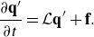 \begin{equation} \frac {\partial \textbf{q}^\prime }{\partial t} = \mathcal{L} \textbf{q}^\prime + \textbf{f}. \end{equation}
We conduct a parametric study for the actuation of constant amplitude (2.20), varying the phase $\phi$
from
$\phi$
from $0$
to
$0$
to $2\pi$
in increments of
$2\pi$
in increments of $\pi /10$
and the amplitude between 0.01 and 0.5 for most of the cases. Then, we conduct a single linear simulation with adaptive actuation amplitude (2.19), using the most effective combination of
$\pi /10$
and the amplitude between 0.01 and 0.5 for most of the cases. Then, we conduct a single linear simulation with adaptive actuation amplitude (2.19), using the most effective combination of $A$
and
$A$
and $\phi$
found in the parametric analysis, to assess whether the receptivity-based actuation indeed fully damps the unstable mode asymptotically. Each linear simulation is initiated using the unstable mode obtained from the LSA as the initial condition with amplitude such that the normalisation condition (2.18) is satisfied, from which both
$\phi$
found in the parametric analysis, to assess whether the receptivity-based actuation indeed fully damps the unstable mode asymptotically. Each linear simulation is initiated using the unstable mode obtained from the LSA as the initial condition with amplitude such that the normalisation condition (2.18) is satisfied, from which both $A$
and
$A$
and $\phi$
are fixed. In the linear simulation, normal modes are decoupled from each other so the time-dependent solution obtained by initialising the solution with a single normal mode reflects the evolution of that particular mode only. As such, linear simulations provide a direct measure of the ability of the actuation based on the receptivity mode to affect the evolution of the unstable mode. To quantitatively asses this effect, we monitor the time-dependent energy of the mode,
$\phi$
are fixed. In the linear simulation, normal modes are decoupled from each other so the time-dependent solution obtained by initialising the solution with a single normal mode reflects the evolution of that particular mode only. As such, linear simulations provide a direct measure of the ability of the actuation based on the receptivity mode to affect the evolution of the unstable mode. To quantitatively asses this effect, we monitor the time-dependent energy of the mode, $(\textbf{q}^\prime, \textbf{q}^\prime)$
. The lowest value
$(\textbf{q}^\prime, \textbf{q}^\prime)$
. The lowest value $(\textbf {q}^\prime, \textbf{q}^\prime)_{min }$
reached by this quantity gives an indication of the damping achieved by the actuation, and the time of occurrence of this minimum measures the time scale over which this damping is achieved, denoted as
$(\textbf {q}^\prime, \textbf{q}^\prime)_{min }$
reached by this quantity gives an indication of the damping achieved by the actuation, and the time of occurrence of this minimum measures the time scale over which this damping is achieved, denoted as $t_f$
. Going back to the example of the continuous casting of alloys as one of the motivations for this work, the unstable mode may not need to be suppressed indefinitely. Instead, maintaining the unstable mode to a low level for the entire duration of the casting operation, which is finite, would be sufficient to ensure it does not impact the final quality of the alloy. Hence the importance of
$t_f$
. Going back to the example of the continuous casting of alloys as one of the motivations for this work, the unstable mode may not need to be suppressed indefinitely. Instead, maintaining the unstable mode to a low level for the entire duration of the casting operation, which is finite, would be sufficient to ensure it does not impact the final quality of the alloy. Hence the importance of $t_f$
is both fundamental and practical.
$t_f$
is both fundamental and practical.
For the simulation case C1 ( $Re=0$
,
$Re=0$
, $Ra=7 \times 10^3$
and
$Ra=7 \times 10^3$
and $k=6$
) (a) Minimum value of the strength of perturbation
$k=6$
) (a) Minimum value of the strength of perturbation $(\textbf{q}^\prime, \textbf{q}^\prime)_{min }$
as a function of the amplitude
$(\textbf{q}^\prime, \textbf{q}^\prime)_{min }$
as a function of the amplitude $A$
and the phase
$A$
and the phase $\phi$
of the linear receptivity-based actuation. (b) Dependence of the time
$\phi$
of the linear receptivity-based actuation. (b) Dependence of the time $t_f$
at which
$t_f$
at which $(\textbf{q}^\prime, \textbf{q}^\prime)_{min }$
occurs on the amplitude
$(\textbf{q}^\prime, \textbf{q}^\prime)_{min }$
occurs on the amplitude $A$
and phase
$A$
and phase $\phi$
. (c) The strength of perturbation
$\phi$
. (c) The strength of perturbation $(\textbf{q}^\prime, \textbf{q}^\prime)$
as a function of time
$(\textbf{q}^\prime, \textbf{q}^\prime)$
as a function of time $t$
for both unforced and forced cases. The inset represents the evolution of both constant amplitude actuation and adaptive actuation from
$t$
for both unforced and forced cases. The inset represents the evolution of both constant amplitude actuation and adaptive actuation from $t=0$
to
$t=0$
to $t \simeq t_f$
.
$t \simeq t_f$
.
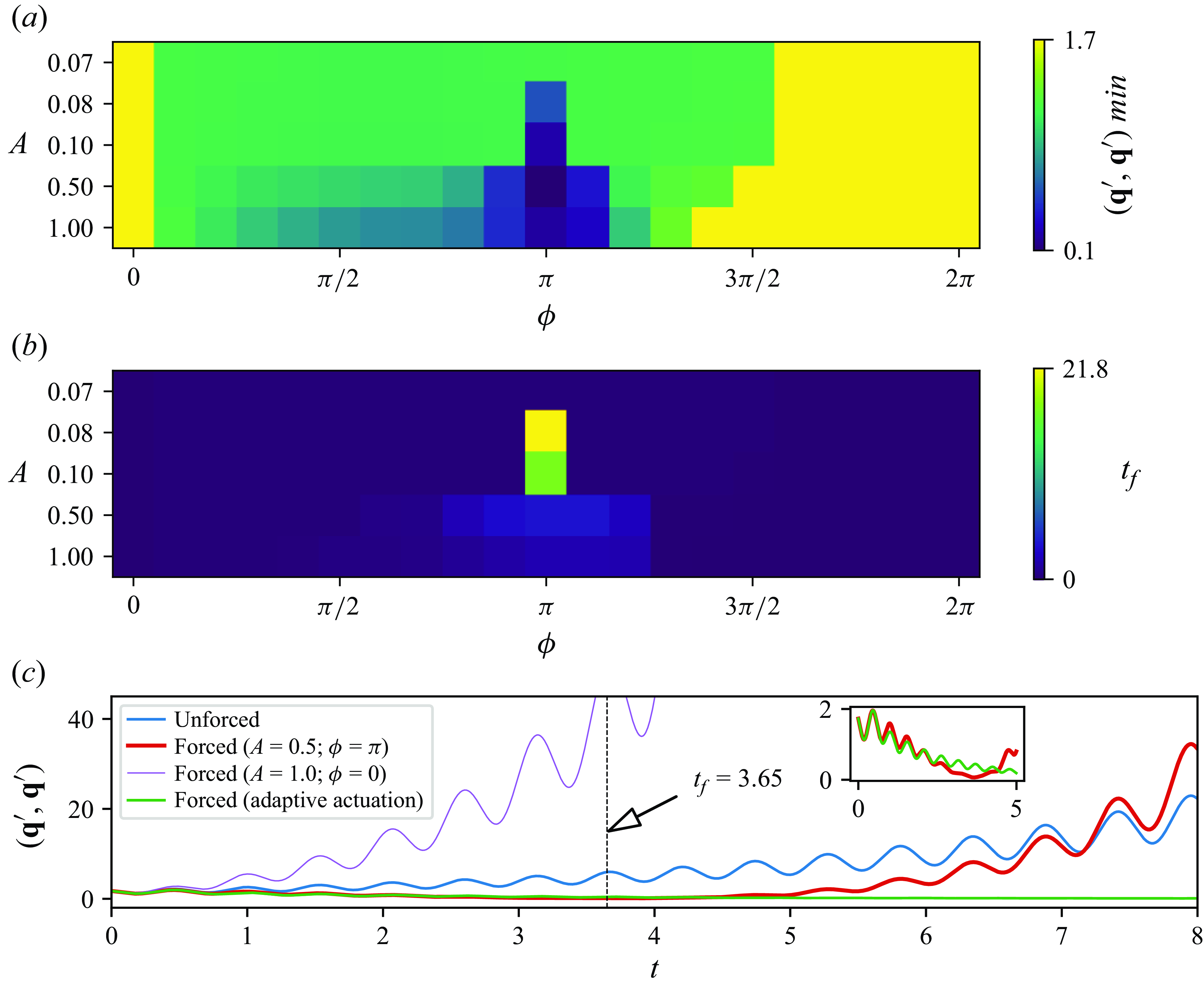
4.2. Analysis of cases C1–C4
We shall now examine the outcome of this approach in each of the C1–C4 cases, defined in § 2.4. Figure 4(c) illustrates four examples of the evolution of $(\textbf{q}^\prime, \textbf{q}^\prime)$
for case C1. The blue curve represents a simulation with no actuation, i.e. one with
$(\textbf{q}^\prime, \textbf{q}^\prime)$
for case C1. The blue curve represents a simulation with no actuation, i.e. one with $A=0$
amplitude. As predicted by LSA, the instability grows exponentially with oscillations of frequency determined by the imaginary part of the mode’s eigenvalue. The red curve represents the case with receptivity-based actuation of amplitude
$A=0$
amplitude. As predicted by LSA, the instability grows exponentially with oscillations of frequency determined by the imaginary part of the mode’s eigenvalue. The red curve represents the case with receptivity-based actuation of amplitude $A=0.5$
and phase
$A=0.5$
and phase $\phi =\pi$
. In this case,
$\phi =\pi$
. In this case, $(\textbf{q}^\prime, \textbf{q}^\prime)$
decreases over time and reaches its minimum value at
$(\textbf{q}^\prime, \textbf{q}^\prime)$
decreases over time and reaches its minimum value at $t_f=3.65$
. For
$t_f=3.65$
. For $t\gt t_f$
,
$t\gt t_f$
, $(\textbf{q}^\prime, \textbf{q}^\prime)$
increases, and crosses the blue curve at
$(\textbf{q}^\prime, \textbf{q}^\prime)$
increases, and crosses the blue curve at $t=7.16$
. Hence, in this particular case, the actuation results in an effective suppression of the instability until
$t=7.16$
. Hence, in this particular case, the actuation results in an effective suppression of the instability until $t=t_f$
. Now, to determine the optimal value of
$t=t_f$
. Now, to determine the optimal value of $A$
and
$A$
and $\phi$
, i.e. values that achieve the smallest value of
$\phi$
, i.e. values that achieve the smallest value of $(\textbf{q}^\prime, \textbf{q}^\prime)_{min }$
, we vary the phase in the range of
$(\textbf{q}^\prime, \textbf{q}^\prime)_{min }$
, we vary the phase in the range of $0$
to
$0$
to $2\pi$
, and for amplitudes between 0.07 and 1.0. The grid map of the corresponding values of
$2\pi$
, and for amplitudes between 0.07 and 1.0. The grid map of the corresponding values of $(\textbf{q}^\prime, \textbf{q}^\prime)_{min }$
is shown in figure 4(a) for case C1. It turns out that
$(\textbf{q}^\prime, \textbf{q}^\prime)_{min }$
is shown in figure 4(a) for case C1. It turns out that $A=0.5$
and
$A=0.5$
and $\phi =\pi$
are the optimal values of amplitude and phase with
$\phi =\pi$
are the optimal values of amplitude and phase with $(\textbf{q}^\prime, \textbf{q}^\prime)_{min } = 0.06$
. Simulation conducted with adaptive actuation (2.19) shows that the unstable mode decays very similarly to the case of constant amplitude actuation until
$(\textbf{q}^\prime, \textbf{q}^\prime)_{min } = 0.06$
. Simulation conducted with adaptive actuation (2.19) shows that the unstable mode decays very similarly to the case of constant amplitude actuation until $t\simeq t_f$
, but continues to decay asymptotically to zero as
$t\simeq t_f$
, but continues to decay asymptotically to zero as $t \to \infty$
. This shows that the receptivity-based actuation indeed suppresses the unstable mode completely.
$t \to \infty$
. This shows that the receptivity-based actuation indeed suppresses the unstable mode completely.
For the simulation case C2 ( $Re=50$
,
$Re=50$
, $Ra=7 \times 10^3$
and
$Ra=7 \times 10^3$
and $k=6$
). (a) Minimum value of the strength of perturbation
$k=6$
). (a) Minimum value of the strength of perturbation $(\textbf{q}^\prime, \textbf{q}^\prime)_{min }$
as a function of the amplitude
$(\textbf{q}^\prime, \textbf{q}^\prime)_{min }$
as a function of the amplitude $A$
and the phase
$A$
and the phase $\phi$
of the linear receptivity-based actuation. (b) Dependence of the time
$\phi$
of the linear receptivity-based actuation. (b) Dependence of the time $t_f$
at which
$t_f$
at which $(\textbf{q}^\prime, \textbf{q}^\prime)_{min }$
occurs on the amplitude
$(\textbf{q}^\prime, \textbf{q}^\prime)_{min }$
occurs on the amplitude $A$
and phase
$A$
and phase $\phi$
. (c) The strength of perturbation
$\phi$
. (c) The strength of perturbation $(\textbf{q}^\prime, \textbf{q}^\prime)$
as a function of time
$(\textbf{q}^\prime, \textbf{q}^\prime)$
as a function of time $t$
for both unforced and forced cases. The inset represents the evolution of both constant amplitude actuation and adaptive actuation from
$t$
for both unforced and forced cases. The inset represents the evolution of both constant amplitude actuation and adaptive actuation from $t=0$
to
$t=0$
to $t \simeq t_f$
.
$t \simeq t_f$
.
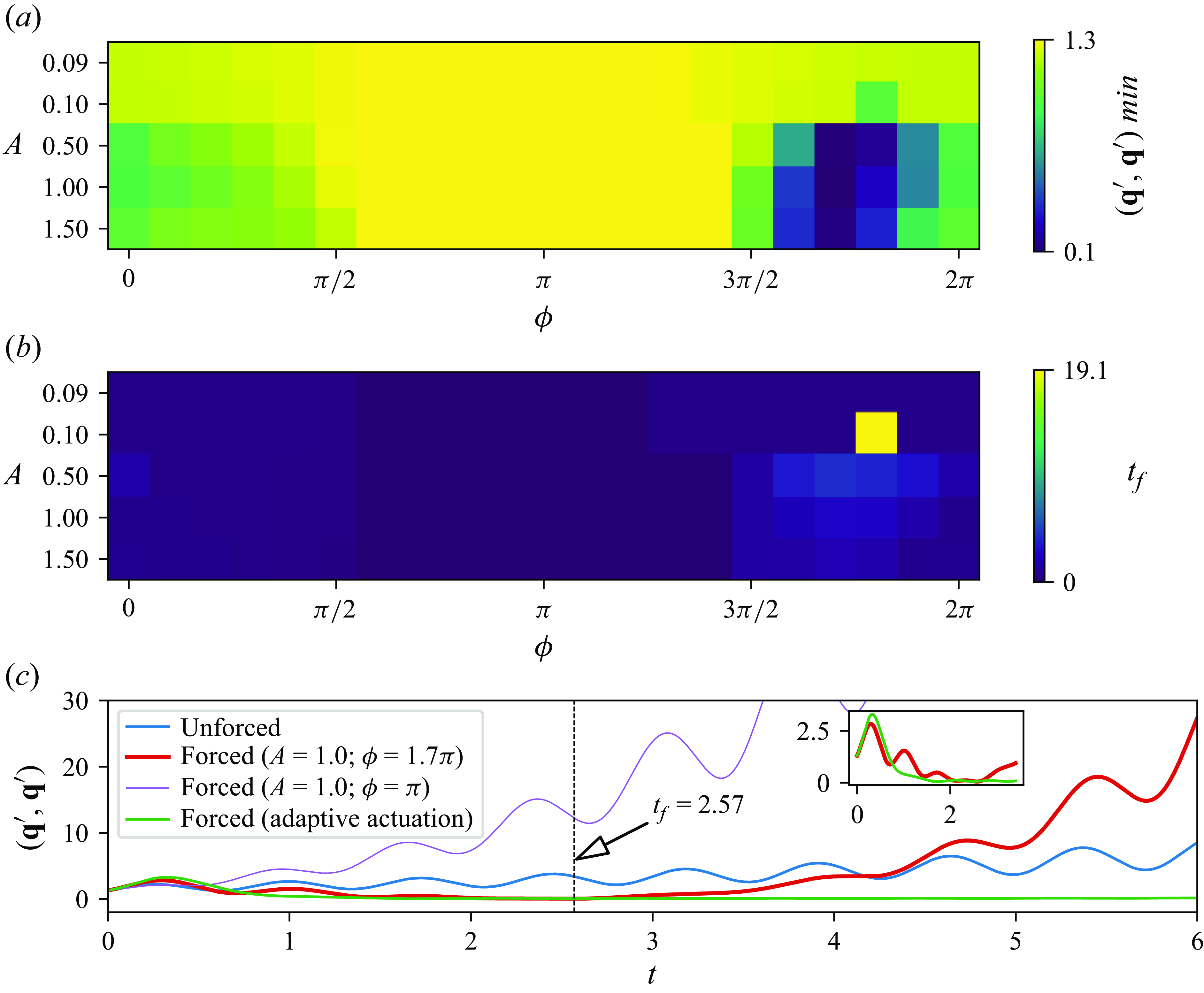
For the simulation case C3 ( $Re=100$
,
$Re=100$
, $Ra=4 \times 10^4$
and
$Ra=4 \times 10^4$
and $k=4$
). (a) Minimum value of the strength of perturbation
$k=4$
). (a) Minimum value of the strength of perturbation $(\textbf{q}^\prime, \textbf{q}^\prime)_{min }$
as a function of the amplitude
$(\textbf{q}^\prime, \textbf{q}^\prime)_{min }$
as a function of the amplitude $A$
and the phase
$A$
and the phase $\phi$
of the linear receptivity-based actuation. (b) Dependence of the time
$\phi$
of the linear receptivity-based actuation. (b) Dependence of the time $t_f$
at which
$t_f$
at which $(\textbf{q}^\prime, \textbf{q}^\prime)_{min }$
occurs on the amplitude
$(\textbf{q}^\prime, \textbf{q}^\prime)_{min }$
occurs on the amplitude $A$
and phase
$A$
and phase $\phi$
. (c) The strength of perturbation
$\phi$
. (c) The strength of perturbation $(\textbf{q}^\prime, \textbf{q}^\prime)$
as a function of time
$(\textbf{q}^\prime, \textbf{q}^\prime)$
as a function of time $t$
for both unforced and forced cases. The inset represents the evolution of both constant amplitude actuation and adaptive actuation from
$t$
for both unforced and forced cases. The inset represents the evolution of both constant amplitude actuation and adaptive actuation from $t=0$
to
$t=0$
to $t \simeq t_f$
.
$t \simeq t_f$
.
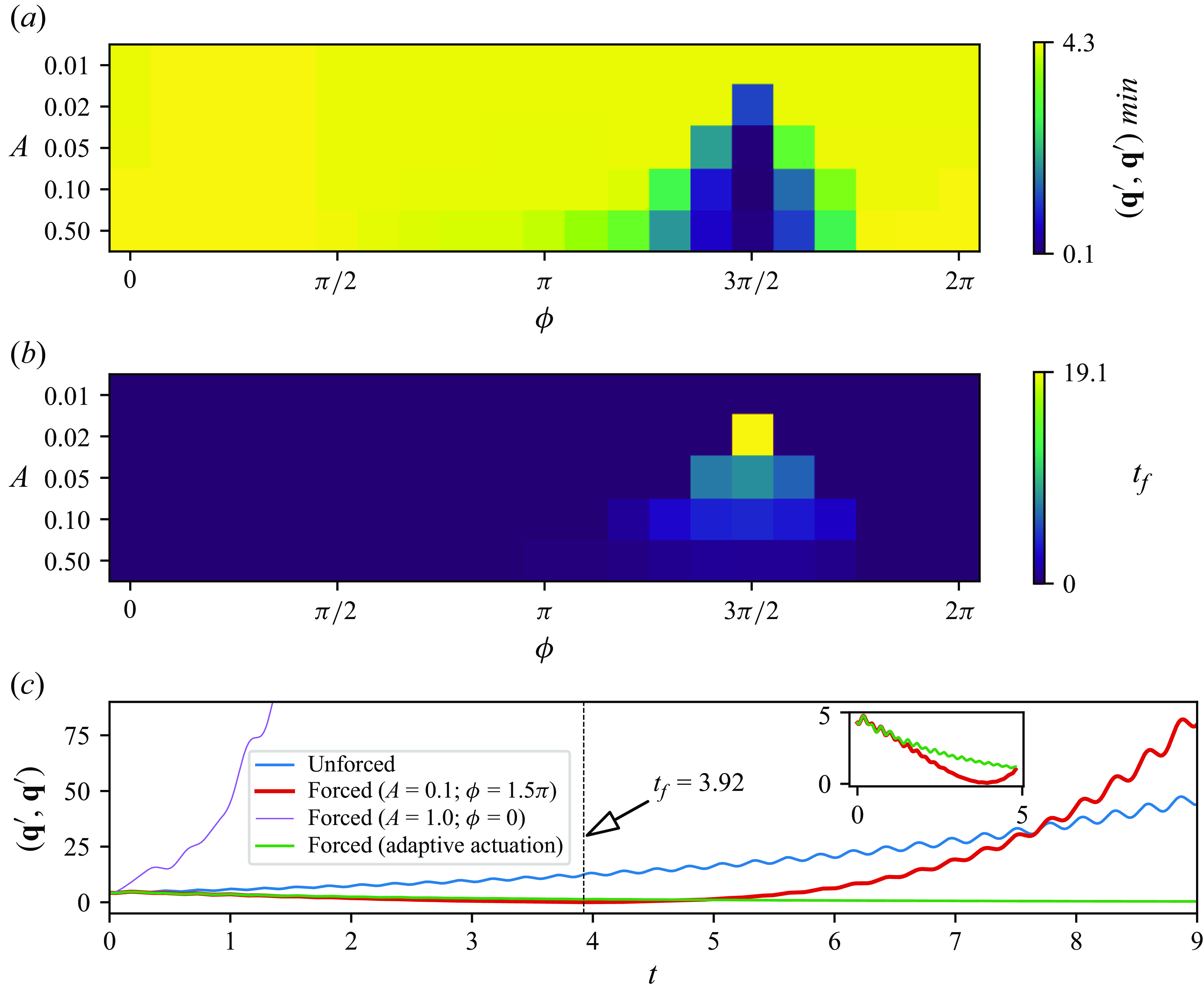
Further calculations were performed for cases C2 and C3, which, despite corresponding to different instability branches, return similar results, presented in figures 5 and 6. As compared with case C1, case C2 has an optimal amplitude that is twice as large, with a phase shift of $1.7\pi$
radians. Therefore, the optimal values are
$1.7\pi$
radians. Therefore, the optimal values are $A=1.0$
and
$A=1.0$
and $\phi =1.7\pi$
. The value of
$\phi =1.7\pi$
. The value of $t_f$
is slightly reduced to 2.57. On the other hand, for case C3, the optimal amplitude is reduced to 0.1, and the optimal phase is shifted to
$t_f$
is slightly reduced to 2.57. On the other hand, for case C3, the optimal amplitude is reduced to 0.1, and the optimal phase is shifted to $1.5\pi$
. The value of
$1.5\pi$
. The value of $t_f$
, however, is slightly increased to 3.93, which implies that the instability can be attenuated for a slightly longer period of time. As in case C1, the adaptive actuation (2.19) leads to a decay similar to the constant amplitude actuation until
$t_f$
, however, is slightly increased to 3.93, which implies that the instability can be attenuated for a slightly longer period of time. As in case C1, the adaptive actuation (2.19) leads to a decay similar to the constant amplitude actuation until $t\simeq t_f$
, but it continues to decay asymptotically to zero as
$t\simeq t_f$
, but it continues to decay asymptotically to zero as $t \to \infty$
, so in cases C2 and C3 too, the receptivity-based actuation fully suppresses the unstable mode.
$t \to \infty$
, so in cases C2 and C3 too, the receptivity-based actuation fully suppresses the unstable mode.
For the simulation case C4 ( $Re=150$
,
$Re=150$
, $Ra=8 \times 10^4$
, and
$Ra=8 \times 10^4$
, and $k=6$
). (a) Minimum value of the strength of perturbation
$k=6$
). (a) Minimum value of the strength of perturbation $(\textbf{q}^\prime, \textbf{q}^\prime)_{min }$
as a function of the amplitude
$(\textbf{q}^\prime, \textbf{q}^\prime)_{min }$
as a function of the amplitude $A$
of the linear receptivity-based actuation. Inset represents the amplitude
$A$
of the linear receptivity-based actuation. Inset represents the amplitude $A=-0.03$
which corresponds to the lowest value of
$A=-0.03$
which corresponds to the lowest value of $(\textbf{q}^\prime, \textbf{q}^\prime)_{min }$
. (b) Dependence of the time
$(\textbf{q}^\prime, \textbf{q}^\prime)_{min }$
. (b) Dependence of the time $t_f$
at which
$t_f$
at which $(\textbf{q}^\prime, \textbf{q}^\prime)_{min }$
occurs on the amplitude
$(\textbf{q}^\prime, \textbf{q}^\prime)_{min }$
occurs on the amplitude $A$
. (c) The strength of perturbation
$A$
. (c) The strength of perturbation $(\textbf{q}^\prime, \textbf{q}^\prime)$
as a function of time
$(\textbf{q}^\prime, \textbf{q}^\prime)$
as a function of time $t$
for both unforced and forced cases. The inset represents the evolution of both constant amplitude actuation and adaptive actuation from
$t$
for both unforced and forced cases. The inset represents the evolution of both constant amplitude actuation and adaptive actuation from $t=0$
to
$t=0$
to $t \simeq t_f$
.
$t \simeq t_f$
.
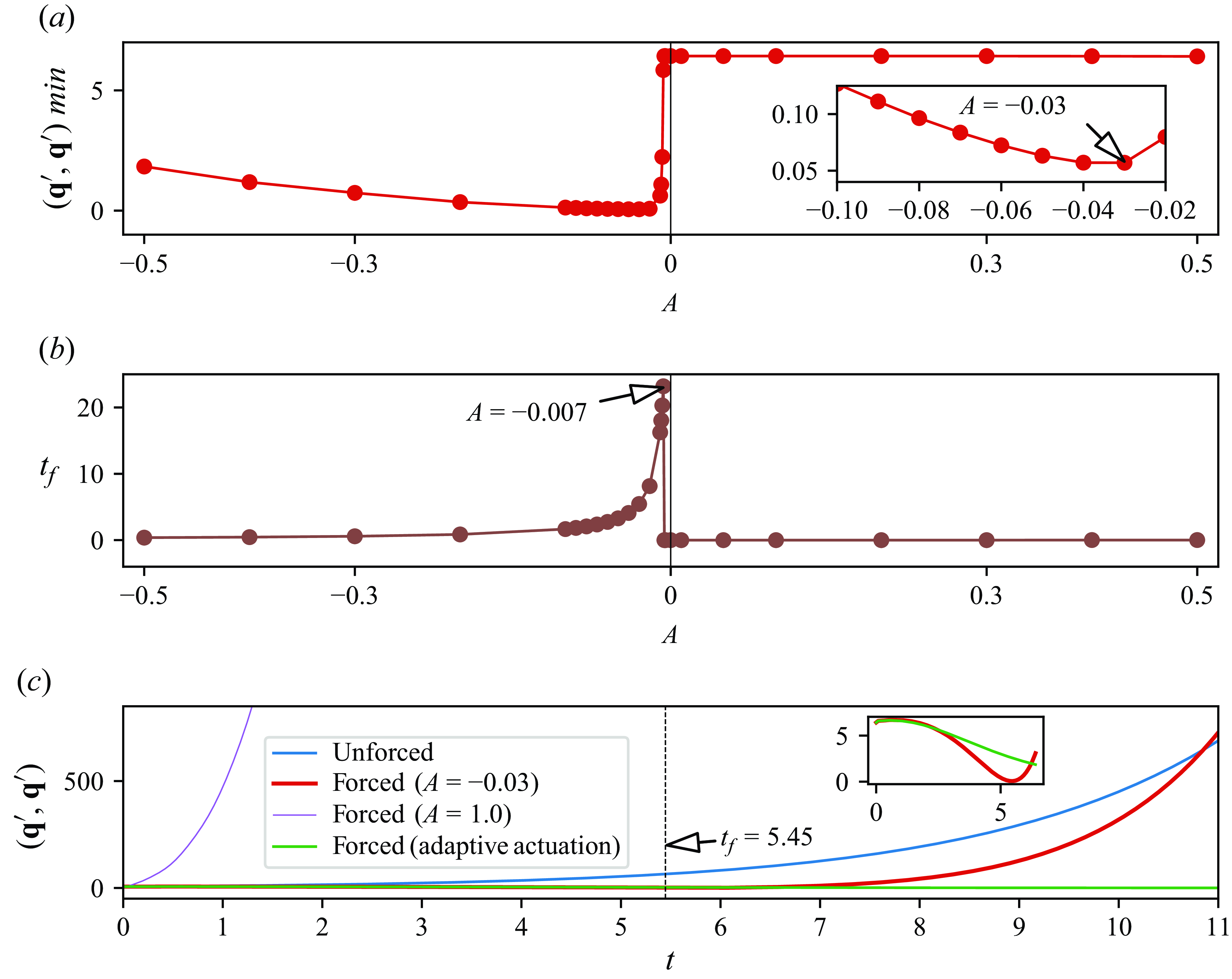
Case C4 differs from the other cases in that the leading eigenmode and its adjoint, which represents receptivity, are non-oscillatory. Consequently, the actuation is also non-oscillatory and we do not need to determine the optimal phase, only the optimal amplitude. In the absence of a phase, the possibility still remains to reverse the actuation, which we incorporated into the sign of $A$
. The variations of
$A$
. The variations of $(\textbf{q}^\prime, \textbf{q}^\prime)_{min }$
with
$(\textbf{q}^\prime, \textbf{q}^\prime)_{min }$
with $A$
are shown in figure 7(a). For
$A$
are shown in figure 7(a). For $A\geq 0$
,
$A\geq 0$
, $(\textbf{q}^\prime, \textbf{q}^\prime)_{min }$
remains very close to the initial value of
$(\textbf{q}^\prime, \textbf{q}^\prime)_{min }$
remains very close to the initial value of $(\textbf{q}^\prime, \textbf{q}^\prime)$
so no suppression is achieved. For
$(\textbf{q}^\prime, \textbf{q}^\prime)$
so no suppression is achieved. For $A\lt 0$
, by contrast, we observe a sudden drop in the value of
$A\lt 0$
, by contrast, we observe a sudden drop in the value of $(\textbf{q}^\prime, \textbf{q}^\prime)_{min }$
at very small amplitudes, with a minimum value at
$(\textbf{q}^\prime, \textbf{q}^\prime)_{min }$
at very small amplitudes, with a minimum value at $A=-0.03$
(see inset of figure 7
a).
$A=-0.03$
(see inset of figure 7
a).
Figure 7(c) shows the evolution of $(\textbf{q}^\prime, \textbf{q}^\prime)$
over time for both the unforced and forced cases with
$(\textbf{q}^\prime, \textbf{q}^\prime)$
over time for both the unforced and forced cases with $A=-0.03$
. It appears that the actuation achieves a suppression of the non-oscillatory mode up to time
$A=-0.03$
. It appears that the actuation achieves a suppression of the non-oscillatory mode up to time $5.45$
. Here again, the adaptive actuation (2.19) suppresses the unstable mode completely and acts over the same time scale
$5.45$
. Here again, the adaptive actuation (2.19) suppresses the unstable mode completely and acts over the same time scale $t_f$
as the constant amplitude actuation.
$t_f$
as the constant amplitude actuation.
4.3. The salient features of the linear response to an actuation of constant amplitude
In all cases, the receptivity-based actuation with adaptive amplitude suppresses the unstable mode asymptotically. This result shows that the theoretical foundations for the receptivity-based instability control are sound. However, the actuation with constant amplitude is more useful in practical situations, but induces a more complex response, which we now discuss in more detail. All four cases show strong similarities, despite the differences in the nature of the unstable modes. First, the linear actuation has a stabilising effect up to a finite time $t_f$
, effectively suppressing the instability. Beyond this point, the unstable mode grows again and at a faster pace than when unforced. This means that for
$t_f$
, effectively suppressing the instability. Beyond this point, the unstable mode grows again and at a faster pace than when unforced. This means that for $t\gt t_f$
, the linear actuation becomes destabilising. The reason is that, since the base flow is fixed in the linear equations we simulate, the actuation’s only effect is to suppress the unstable mode. Once the mode is suppressed, the system is back to the equilibrium point defined by the steady base flow. The actuation then acts as an additional force, moving the system away from this equilibrium. Nonlinear simulations are required to verify whether the base flow is indeed affected by the actuation and whether the phenomenology observed in the linear framework is indeed valid. Table 3 shows that
$t\gt t_f$
, the linear actuation becomes destabilising. The reason is that, since the base flow is fixed in the linear equations we simulate, the actuation’s only effect is to suppress the unstable mode. Once the mode is suppressed, the system is back to the equilibrium point defined by the steady base flow. The actuation then acts as an additional force, moving the system away from this equilibrium. Nonlinear simulations are required to verify whether the base flow is indeed affected by the actuation and whether the phenomenology observed in the linear framework is indeed valid. Table 3 shows that $t_f$
remains of the order of the inverse of the growth rate of the unstable mode, as the ratio
$t_f$
remains of the order of the inverse of the growth rate of the unstable mode, as the ratio $\sigma t_f$
remains of the order of unity for all suppression-optimising cases. The term ‘suppression-optimising’ refers to seeking the amplitude and phase of the forcing that achieve the maximum reduction in mode amplitude. The reduction in mode amplitude achieved at
$\sigma t_f$
remains of the order of unity for all suppression-optimising cases. The term ‘suppression-optimising’ refers to seeking the amplitude and phase of the forcing that achieve the maximum reduction in mode amplitude. The reduction in mode amplitude achieved at $t=t_f$
is of approximatively two orders of magnitudes (see table 3) for the suppression-optimising cases. This suggests that the actuation is more effective when applied for a finite time
$t=t_f$
is of approximatively two orders of magnitudes (see table 3) for the suppression-optimising cases. This suggests that the actuation is more effective when applied for a finite time $t_f$
, then stopped until the unstable mode regrows to its initial amplitude (i.e. during a time
$t_f$
, then stopped until the unstable mode regrows to its initial amplitude (i.e. during a time $\sim \sigma ^{-1}$
), at which point the procedure can be repeated. Whether this strategy is realistic depends on how this pattern is affected by nonlinearities.
$\sim \sigma ^{-1}$
), at which point the procedure can be repeated. Whether this strategy is realistic depends on how this pattern is affected by nonlinearities.
The normalised value of $t_f$
with respect to the growth rate
$t_f$
with respect to the growth rate $\sigma$
for various suppression-optimising and time-optimising simulation cases. Comparison of
$\sigma$
for various suppression-optimising and time-optimising simulation cases. Comparison of $(\textbf{q}^\prime, \textbf{q}^\prime)_{min }$
relative to the initial value of
$(\textbf{q}^\prime, \textbf{q}^\prime)_{min }$
relative to the initial value of $(\textbf{q}^\prime, \textbf{q}^\prime)$
is shown for each suppression-optimising and time-optimising simulation cases.
$(\textbf{q}^\prime, \textbf{q}^\prime)$
is shown for each suppression-optimising and time-optimising simulation cases.
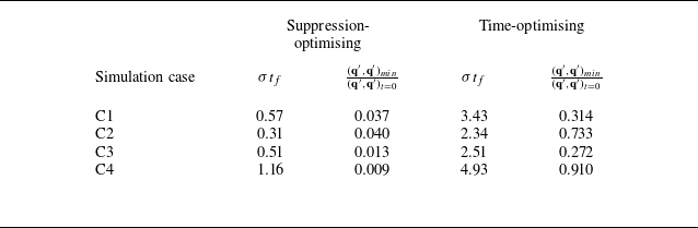
This pattern also raises the question of whether instead of applying suppression-optimising, it may be beneficial to seek configurations that achieve the largest value of $t_f$
so as to maximise the time during which the suppression is effective. The term ‘time-optimising’ is introduced to denote the search for amplitude and phase settings that maximise the value of
$t_f$
so as to maximise the time during which the suppression is effective. The term ‘time-optimising’ is introduced to denote the search for amplitude and phase settings that maximise the value of $t_f$
. The corresponding optimal values are shown on figures 4(b), 5(b), 6(b) and 7(b). Unsurprisingly, actuation parameters optimising the suppression and
$t_f$
. The corresponding optimal values are shown on figures 4(b), 5(b), 6(b) and 7(b). Unsurprisingly, actuation parameters optimising the suppression and $t_f$
differ. We shall compare how both optimals perform on the nonlinear response in the next section.
$t_f$
differ. We shall compare how both optimals perform on the nonlinear response in the next section.
In addition to identifying optimal suppression parameters, our results highlight that certain combinations of amplitude and phase can instead enhance instability. For instance, as shown in figure 4(c), the case $A=1$
and
$A=1$
and $\phi =0$
leads to the most destabilising effect for
$\phi =0$
leads to the most destabilising effect for $Re=0$
, and similarly, as shown in figure 6(c), for
$Re=0$
, and similarly, as shown in figure 6(c), for $ Re=100$
. In contrast, for
$ Re=100$
. In contrast, for $Re=50$
(figure 5
c), the configuration
$Re=50$
(figure 5
c), the configuration $A=1$
and
$A=1$
and $\phi =\pi$
is more destabilising than
$\phi =\pi$
is more destabilising than $ A=1$
and
$ A=1$
and $ \phi =0$
. This observation underscores the importance of carefully selecting both the amplitude and phase in actuation design, as an inappropriate choice can inadvertently amplify perturbations rather than suppressing them.
$ \phi =0$
. This observation underscores the importance of carefully selecting both the amplitude and phase in actuation design, as an inappropriate choice can inadvertently amplify perturbations rather than suppressing them.
5. Nonlinear response to an actuation based on receptivity
5.1. Methodology
The linear simulations confirmed that an actuation designed from the topology of the receptivity, with a frequency matched to the leading eigenmode was indeed capable of stifling the linear mechanism responsible for the growth of the leading eigenmode. We also identified the relative amplitude and phase that maximised its suppression. In reality, the finite amplitude of the perturbation, whether subject to the actuation or not, activates a nonlinear response of the system. Although nonlinearities may not measurably deflect the perturbation’s evolution in its early stages, when its amplitude is still small, it is likely to govern its dynamics at longer time scales, especially at the point where the actuation ceases to be efficient. For this reason, the nonlinear effects are essential to determine how effective the actuation may be at suppressing instabilities, and how long it may remain so.
Including the nonlinear dynamics, however, raises several technical difficulties. First, the optimal amplitude and phase were determined without any consideration of nonlinearity, so we may question whether these remain optimal for the nonlinear evolution. The answer lies partly in how the suppression is assessed. Following the approach we adopted in the linear study, we sought the point of lowest amplitude for the leading eigenmode and the time of this minimum. Since the evolution from an infinitesimal perturbation to that point involves only very small amplitudes, it is legitimate to assume that nonlinearities would play little role there and that, consequently, the linear and the nonlinear evolutions would remain very similar during this phase (Drazin & Reid Reference Drazin and Reid2004). One should, however, keep in mind that if phase and amplitude were sought so as to optimise the saturated state of the evolution, the full nonlinear equations would need to be included in the optimisation process (Pringle, Willis & Kerswell Reference Pringle, Willis and Kerswell2012). However, our specific purpose of understanding the influence of the nonlinear effects is better served by keeping a similar approach to the linear study. Additionally, since the linear study showed that the growth of the leading eigenmode was only effectively suppressed until $t=t_f$
, we shall only apply the actuation up to that time, and let the flow evolve freely after that time.
$t=t_f$
, we shall only apply the actuation up to that time, and let the flow evolve freely after that time.
Second, the definition of the initial conditions for the nonlinear problem differs from the linear one: the linear equations indeed return the same evolution regardless of the amplitude of the initial condition (up to a multiplicative factor), and only the relative amplitude and phase of the actuation mattered. To transpose our approach into the nonlinear framework, we shall also specify the amplitude and phase of the actuation relative to the perturbation. In the nonlinear equations, however, if the unstable mode is left to grow ‘naturally’ from noise, its amplitude and phase are not specified in the initial condition, so actuation cannot be fixed a priori. A workaround would be to let the unstable mode develop up to a trigger amplitude, where both amplitude and phase can be measured, and then apply the optimal actuation based on these. Indeed, such an approach would be required in a real process where the onset of instability would need to be detected for the actuation to be activated. For instance, electromagnetic sensors (Thomas et al. Reference Thomas, Yuan, Sivaramakrishnan, Shi, Vanka and Assar2001; Cho & Thomas Reference Cho and Thomas2019) can detect the onset of such instabilities. Since our previous study of the free nonlinear evolution of the leading eigenmode confirmed that it emerged naturally from noise (Kumar & Pothérat Reference Kumar and Pothérat2020), we shall directly initiate the nonlinear simulation with the leading eigenmode set to an amplitude such its ratio to the base flow,
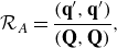 \begin{equation} \mathcal{R}_A = \frac {(\textbf{q}^\prime, \textbf{q}^\prime)}{(\textbf{Q},\textbf{Q})}, \end{equation}
remains much smaller than unity (see table 4). Here, $\textbf{Q}=(\textbf{U}, \bar {T})^\top$
represents the steady base flow. Note that for the nonlinear simulations,
$\textbf{Q}=(\textbf{U}, \bar {T})^\top$
represents the steady base flow. Note that for the nonlinear simulations, $\textbf{q}^\prime$
is obtained by subtracting the base flow from the entire flow field.
$\textbf{q}^\prime$
is obtained by subtracting the base flow from the entire flow field.
Parameters of our numerical calculations: Reynolds number $Re$
, Rayleigh number
$Re$
, Rayleigh number $Ra$
, order of polynomial
$Ra$
, order of polynomial $N$
, time step
$N$
, time step $\Delta t$
. Here amplitude ratio
$\Delta t$
. Here amplitude ratio $\mathcal{R}_A$
, the forcing cutoff time
$\mathcal{R}_A$
, the forcing cutoff time $t_f$
, nonlinear efficiency time
$t_f$
, nonlinear efficiency time $t_{{ eff}}=t_2-t_1$
and actuation efficiency
$t_{{ eff}}=t_2-t_1$
and actuation efficiency $\eta _a=t_R/t_f$
based on recovery time
$\eta _a=t_R/t_f$
based on recovery time $t_R$
such that
$t_R$
such that $(\textbf{q}^\prime, \textbf{q}^\prime)_{t=t_R}=(\textbf{q}^\prime, \textbf{q}^\prime)_{t=0}$
for the 3-D DNS.
$(\textbf{q}^\prime, \textbf{q}^\prime)_{t=t_R}=(\textbf{q}^\prime, \textbf{q}^\prime)_{t=0}$
for the 3-D DNS.
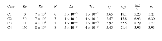
As a function of time $t$
, the nonlinear evolution of the perturbation energy
$t$
, the nonlinear evolution of the perturbation energy $(\textbf{q}^\prime, \textbf{q}^\prime)$
, in the simulation cases (a) C1, (b) C2, (c) C3 and (d) C4, without actuation (blue), with actuation maximising
$(\textbf{q}^\prime, \textbf{q}^\prime)$
, in the simulation cases (a) C1, (b) C2, (c) C3 and (d) C4, without actuation (blue), with actuation maximising $t_f$
(orange) and with actuation achieving maximum reduction of energy (red).
$t_f$
(orange) and with actuation achieving maximum reduction of energy (red).
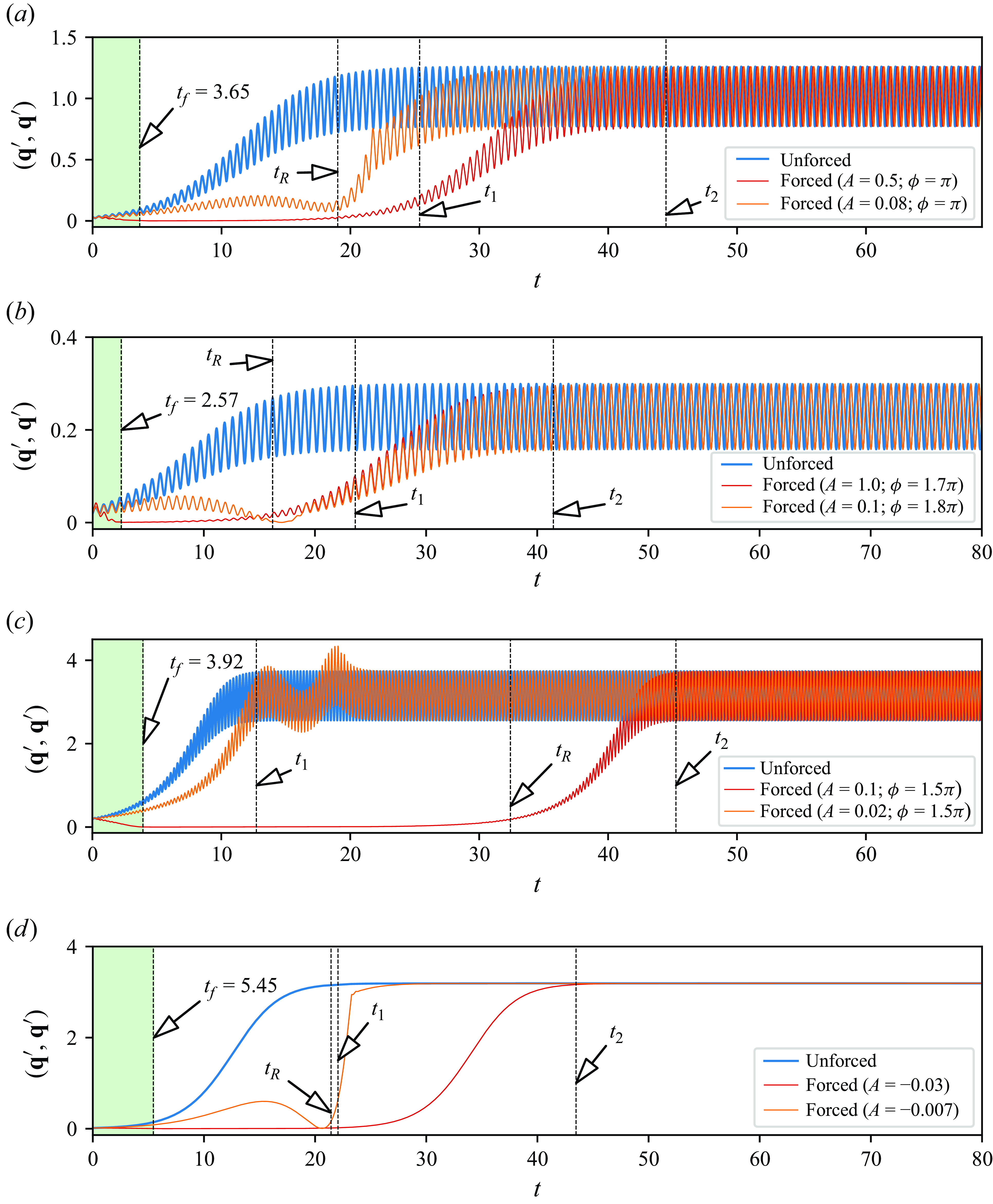
5.2. Analysis of cases C1–C4
The evolution of the perturbation with and without actuation for case C1 is shown in figure 8(a). The blue curve illustrates the free nonlinear evolution with the flow initialised with the leading eigenmode for case C1 and no actuation applied. Initially, the energy of the perturbation $(\textbf{q}^\prime, \textbf{q}^\prime)$
grows exponentially, as predicted by the linear theory, and this confirms that nonlinear effects do not affect the early stages. These indeed induce a saturation at
$(\textbf{q}^\prime, \textbf{q}^\prime)$
grows exponentially, as predicted by the linear theory, and this confirms that nonlinear effects do not affect the early stages. These indeed induce a saturation at $t=t_1=25.4$
. The envelope of the curve provides an estimate of the saturation time, denoted as
$t=t_1=25.4$
. The envelope of the curve provides an estimate of the saturation time, denoted as $t_1$
. We consider the saturation time to be reached when the derivative of the envelope with respect to time falls below
$t_1$
. We consider the saturation time to be reached when the derivative of the envelope with respect to time falls below $10^{-3}$
. The red curve represents the evolution of the perturbation for the same initial conditions, but this time, with the suppression-optimising actuation applied as we just described. Until
$10^{-3}$
. The red curve represents the evolution of the perturbation for the same initial conditions, but this time, with the suppression-optimising actuation applied as we just described. Until $t \approx 10$
, the actuation results in a decrease of the perturbation’s amplitude, after which the perturbation begins to grow slowly. Interestingly, the decay of the perturbation continues well beyond the time of minimum amplitude found in the linear simulation. Since, however, nonlinear effects are not expected to play a role for such low amplitudes, as suggested by the exponential form of the actuation-free evolution, the difference more likely results from switching off the actuation at
$t \approx 10$
, the actuation results in a decrease of the perturbation’s amplitude, after which the perturbation begins to grow slowly. Interestingly, the decay of the perturbation continues well beyond the time of minimum amplitude found in the linear simulation. Since, however, nonlinear effects are not expected to play a role for such low amplitudes, as suggested by the exponential form of the actuation-free evolution, the difference more likely results from switching off the actuation at $t_f$
in the nonlinear simulations. Given the very low amplitude of the perturbation around
$t_f$
in the nonlinear simulations. Given the very low amplitude of the perturbation around $t=t_f$
, the system remains governed by linear dynamics so the reason for the extended period of suppression is that exponential growth from such a low level of perturbation simply extends over a longer period of time. This suggests that applying the actuation beyond the time of maximum growth suppression in fact promotes the growth of the eigenmode. As such, switching off the actuation at
$t=t_f$
, the system remains governed by linear dynamics so the reason for the extended period of suppression is that exponential growth from such a low level of perturbation simply extends over a longer period of time. This suggests that applying the actuation beyond the time of maximum growth suppression in fact promotes the growth of the eigenmode. As such, switching off the actuation at $t_f$
is optimal. The underlying suppression strategy, is then to suppress the leading eigenmode down to the lowest possible amplitude so that the linear mechanism takes as long as possible to act. The nonlinear dynamics only provide a measure of when this strategy ceases to be effective.
$t_f$
is optimal. The underlying suppression strategy, is then to suppress the leading eigenmode down to the lowest possible amplitude so that the linear mechanism takes as long as possible to act. The nonlinear dynamics only provide a measure of when this strategy ceases to be effective.
Indeed, after $t \approx 20$
, the exponential growth becomes sufficient to activate nonlinearities and the perturbation amplitude reaches nonlinear saturation at
$t \approx 20$
, the exponential growth becomes sufficient to activate nonlinearities and the perturbation amplitude reaches nonlinear saturation at $t=t_2$
(
$t=t_2$
( $t_2$
is calculated using the same method as
$t_2$
is calculated using the same method as $t_1$
by analysing the envelope of the curve). In order to estimate the effectiveness of the actuation at suppressing the instability, we define the nonlinear efficiency time,
$t_1$
by analysing the envelope of the curve). In order to estimate the effectiveness of the actuation at suppressing the instability, we define the nonlinear efficiency time, $t_{{ eff}}=t_2 - t_1$
, which for case C1 is
$t_{{ eff}}=t_2 - t_1$
, which for case C1 is $19.1 \simeq 5.23t_f$
. In other words, the actuation prevents nonlinear saturation during
$19.1 \simeq 5.23t_f$
. In other words, the actuation prevents nonlinear saturation during $5.23$
times the duration of its application, i.e. it approximately doubles the time to saturation. Even more interestingly, the unstable mode returns to its initial amplitude at a time
$5.23$
times the duration of its application, i.e. it approximately doubles the time to saturation. Even more interestingly, the unstable mode returns to its initial amplitude at a time $t_R$
,
$t_R$
, $\eta _a=5.21$
times longer than
$\eta _a=5.21$
times longer than $t_f$
, so that it could potentially be indefinitely maintained at that level by applying the actuation during
$t_f$
, so that it could potentially be indefinitely maintained at that level by applying the actuation during $t_f$
every
$t_f$
every $\eta _at_f$
, which costs
$\eta _at_f$
, which costs $\eta _a$
less energy than applying the actuation continuously. These results are very encouraging since they validate the linear approach, and show that the receptivity forcing obtained from the linear analysis is indeed capable of suppressing the growth of the instability in the full nonlinear system for a long time, not only compared with the time scale of growth of the instability and to the duration of the actuation
$\eta _a$
less energy than applying the actuation continuously. These results are very encouraging since they validate the linear approach, and show that the receptivity forcing obtained from the linear analysis is indeed capable of suppressing the growth of the instability in the full nonlinear system for a long time, not only compared with the time scale of growth of the instability and to the duration of the actuation $t_f$
.
$t_f$
.
In addition to applying actuation based on the minimum value of $(\textbf{q}^\prime, \textbf{q}^\prime)$
, we also tested the actuation strategy based on the forcing maximising
$(\textbf{q}^\prime, \textbf{q}^\prime)$
, we also tested the actuation strategy based on the forcing maximising $t_f$
. For case C1, the highest
$t_f$
. For case C1, the highest $t_f$
value of 21.8 is achieved for
$t_f$
value of 21.8 is achieved for $A=0.08$
and
$A=0.08$
and $\phi =\pi$
. The simulation corresponding to these parameters is depicted by the orange curve in figure 8(a). Interestingly, the perturbation energy remains below that of the unforced case until around
$\phi =\pi$
. The simulation corresponding to these parameters is depicted by the orange curve in figure 8(a). Interestingly, the perturbation energy remains below that of the unforced case until around $t \approx 20$
, yet it consistently stays higher than that of the mode with suppression-optimising actuation (
$t \approx 20$
, yet it consistently stays higher than that of the mode with suppression-optimising actuation ( $A=0.5$
), before reaching nonlinear saturation. Since the perturbation energy for
$A=0.5$
), before reaching nonlinear saturation. Since the perturbation energy for $A=0.08,\phi =\pi$
exceeds that of
$A=0.08,\phi =\pi$
exceeds that of $A=0.5, \phi =\pi$
, its nonlinear saturation occurs prior to the case of
$A=0.5, \phi =\pi$
, its nonlinear saturation occurs prior to the case of $A=0.5$
. This means that suppression-optimising actuation outperforms time-optimising actuation.
$A=0.5$
. This means that suppression-optimising actuation outperforms time-optimising actuation.
Case C2 returned exactly the same phenomenology for the suppression-optimising actuation, despite the difference in the nature of the leading eigenmodes (see figure 8
b). The values of $t_{{ eff}}/t_f$
and
$t_{{ eff}}/t_f$
and $\eta _a$
are not significantly different than for case C1, but the time-optimising actuation incurs a different behaviour: although the unstable mode does not initially decay, it decays briefly at a much later time than for the actuation optimising suppression, down to a similar level. Shortly after, however, both curves practically coincide and simultaneously evolve to saturation. In this sense both actuations perform equally well: this is the only case where the suppression-optimising actuation does not significantly outperform the time-optimising actuation. Nevertheless, since the perturbation remains at a much lower level in the initial stages of evolution for the suppression-optimising actuation, it is still overall better at suppressing the unstable mode.
$\eta _a$
are not significantly different than for case C1, but the time-optimising actuation incurs a different behaviour: although the unstable mode does not initially decay, it decays briefly at a much later time than for the actuation optimising suppression, down to a similar level. Shortly after, however, both curves practically coincide and simultaneously evolve to saturation. In this sense both actuations perform equally well: this is the only case where the suppression-optimising actuation does not significantly outperform the time-optimising actuation. Nevertheless, since the perturbation remains at a much lower level in the initial stages of evolution for the suppression-optimising actuation, it is still overall better at suppressing the unstable mode.
Case C3 also produced the same phenomenology shown on figure 8(c), but with increased values of $t_{{ eff}}/t_f=8.29$
and
$t_{{ eff}}/t_f=8.29$
and $\eta _a=8.27$
, i.e. with a much higher efficiency of the suppression-optimising actuation. By contrast with case C2, however, the time-optimising actuation is practically ineffective at suppressing the unstable mode as its amplitude grows to saturation barely later than without any actuation.
$\eta _a=8.27$
, i.e. with a much higher efficiency of the suppression-optimising actuation. By contrast with case C2, however, the time-optimising actuation is practically ineffective at suppressing the unstable mode as its amplitude grows to saturation barely later than without any actuation.
Lastly, we applied constant actuations in the nonlinear simulation of case C4, since the unstable mode is non-oscillatory. Once again, we used the unstable mode as the initial condition. The non-oscillatory nature of the mode does not seem to play a role as the evolution of the mode’s energy in all three simulations, without actuation, with suppression-optimised actuation and with time-optimising actuation show very similar features to cases C1 and C3, with $t_{{ eff}}/t_f \approx \eta _a=3.93$
.
$t_{{ eff}}/t_f \approx \eta _a=3.93$
.
5.3. The salient features of the nonlinear evolution
The overall outcome of the nonlinear simulations is that the phenomenology seen in the linear simulation remains valid until the nonlinear effects become important and crucially, this happens when the saturation starts. If an actuation based on the adjoint mode, applied up to the time of maximum suppression $t_f$
the unstable mode does not regain its initial amplitude until a time
$t_f$
the unstable mode does not regain its initial amplitude until a time $\eta _a t_f$
, roughly an order of magnitude longer than
$\eta _a t_f$
, roughly an order of magnitude longer than $t_f$
(
$t_f$
( $\eta _a=8.27$
in the most favourable case C3), so as long as the amplitude and phase of the actuation are optimised for suppression (and not for
$\eta _a=8.27$
in the most favourable case C3), so as long as the amplitude and phase of the actuation are optimised for suppression (and not for $t_f$
). Until that point, the evolution follows mostly the linear dynamics, as the energy of the unstable mode remains small compared with that of the base flow. The nonlinear effects act shortly after this time, and when they do so, they incur growth up to the same point of saturation as when no actuation is applied.
$t_f$
). Until that point, the evolution follows mostly the linear dynamics, as the energy of the unstable mode remains small compared with that of the base flow. The nonlinear effects act shortly after this time, and when they do so, they incur growth up to the same point of saturation as when no actuation is applied.
In light of this behaviour, an on–off control strategy could offer a viable control strategy. Repeating a sequence where the suppression-optimising actuation is applied until $t_f$
, then switched off to let the flow evolve until
$t_f$
, then switched off to let the flow evolve until $\eta _a t_f$
, may indefinitely keep the flow evolution in the linear regime, where the actuation remains effective. Thus, this strategy may confine oscillations to very small amplitudes for an arbitrary length of time. Though, this strategy needs to be further explored to assess how feasible this approach is in practical applications.
$\eta _a t_f$
, may indefinitely keep the flow evolution in the linear regime, where the actuation remains effective. Thus, this strategy may confine oscillations to very small amplitudes for an arbitrary length of time. Though, this strategy needs to be further explored to assess how feasible this approach is in practical applications.
6. Conclusions
Inspired by the process of continuous casting of liquid metal alloy, we sought to model the suppression of oscillations in mixed baroclinic convection in a nearly hemispherical cavity. This problem offered us an opportunity to assess the feasibility of suppressing oscillatory instabilities by means of an actuation modelled on the receptivity map of unstable modes. Doing so led us to consider four canonical cases spanning the three branches of instability for this problem (Kumar & Pothérat Reference Kumar and Pothérat2020): a purely convective flow subject to a supercritical oscillatory instability (case C1); a mixed convective flow subject to a supercritical oscillatory instability (case C2); a mixed convective flow subject to a subcritical oscillatory instability (case C3); a mixed convective flow subject to a supercritical non-oscillatory instability (case C4).
For this, we first identified the receptivity map for each of these cases. We found that as the intensity of the inflow increases, the region of receptivity becomes increasingly concentrated near the inlet surface, i.e. increasingly favourable in the industrial context where immersing an actuator in the bulk of the melt over extended periods of time is not a feasible option. To gain insight into the instability mechanism, we analysed the sensitivity tensor. We found that for the low Prandtl number of liquid metals, the temperature does not respond to any actuation feedback, whether thermal or mechanical, whereas the velocity field is responsive to both thermal and mechanical actuation. This is understandable since thermal diffusion acts nearly two orders of magnitude faster than viscous diffusion. As such, acting on the temperature field would require a mechanism ${O}(Pr)$
faster than one acting on the velocity field. For C2–C4, the sensitivity map was located in the lower-half of the domain, hence physically disconnected from the receptivity map. The disconnect was less obvious in case C1, but still present, despite a slight overlap between the two maps. This indicates that an actuation in the receptivity region would act on the amplitude of the unstable mode but not affect its eigenvalue, which would react to a forcing aligned with the sensitivity map. With these results in hand, we performed linear and nonlinear simulations of the evolution of the unstable mode with and without actuation to answer the four questions set out in the introduction.
${O}(Pr)$
faster than one acting on the velocity field. For C2–C4, the sensitivity map was located in the lower-half of the domain, hence physically disconnected from the receptivity map. The disconnect was less obvious in case C1, but still present, despite a slight overlap between the two maps. This indicates that an actuation in the receptivity region would act on the amplitude of the unstable mode but not affect its eigenvalue, which would react to a forcing aligned with the sensitivity map. With these results in hand, we performed linear and nonlinear simulations of the evolution of the unstable mode with and without actuation to answer the four questions set out in the introduction.
-
(i) Since, for all cases (except case C1), the area of receptivity is located near the inflow surface, the most efficient way to act on the instability in practice is to modify the inflow. This area is one of the most accessible in casting devices, so this result is favourable to the application. It must, nevertheless, be understood in the context of the simplified model we are considering here, and the question remains open regarding how the receptivity area would change in a more realistic geometry.
-
(ii) Implementing a thermomechanical actuation modelled on the topology of the adjoint to the unstable mode to be suppressed (i.e. its receptivity map) led to a suppression of the unstable eigenmode. To find this result, we scanned possible values of the amplitude and phase of the actuation with respect to the unstable mode. In doing so, we found that it was always possible to find a combination of amplitude and phase of the actuation leading to a significant suppression of the unstable mode. Typically, its energy could be reduced by two orders of magnitude in all four cases.
-
(iii) If kept at a constant amplitude, the actuation only had a stabilising effect during a finite time
$t_f$
of the order of the inverse growth rate of the unstable mode
$\sigma ^{-1}$
, after which linear simulations proved it to be destabilising, in the sense that it enhances the growth of the unstable mode, compared with the simulations without actuation. The reason for this rebound is that, once the instability is suppressed, the actuation acts as an extra force driving the system away from the equilibrium point corresponding to the base flow. This led us to consider two strategies for the design of the actuation: one where amplitude and phase of the actuation are chosen to optimise the suppression of the mode’s energy (suppression-optimising actuation), and one optimising
$t_f$
, i.e. for which the decay of the unstable mode is the longest (time-optimising actuation). On the other hand, if the amplitude of the actuation was kept proportional to the time-dependent amplitude of the unstable mode all along its evolution, the actuation based on receptivity asymptotically led to the full suppression of the unstable mode. Although this method is more difficult to implement in practice, it demonstrates that an actuation based on the receptivity map effectively suppresses the unstable mode. -
(iv) To evaluate the influence of nonlinearities and verify if the actuation led to a modification of the base flow and its corresponding equilibrium point, we calculated the evolution of the unstable mode through the full nonlinear governing equations, with either type of actuation applied during
$t_f$
, after which the flow was left to evolve freely. With suppression-optimising actuation, the energy of the unstable mode always decayed well beyond
$t_f$
before it slowly regrew, to recover its initial amplitude at a time
$\eta _a t_f$
typically an order of magnitude greater than
$t_f$
. In that sense
$\eta _a$
measures the efficiency of the actuation. Time-optimised actuation always led to significantly lower values of
$\eta _a$
, and even to no suppression at all in case C3. Shortly after
$\eta _a t_f$
, nonlinearities incurred a rapid growth leading to a saturation at the same level as nonlinear simulations without actuation. In all cases, however, the suppression phase followed the prediction of the linear simulation where the base flow was fixed. This confirmed that the base flow is not measurably affected by the actuation and confirms that actuations based on the receptivity map acts on the unstable mode only.


The absolute value of the components of the sensitivity tensor $S_{ij} = \hat {\textbf {q}}_i \hat {\textbf {q}}_j^*$
for the simulation case C1 (
$S_{ij} = \hat {\textbf {q}}_i \hat {\textbf {q}}_j^*$
for the simulation case C1 ( $Re=0$
,
$Re=0$
, $Ra=7 \times 10^3$
and
$Ra=7 \times 10^3$
and $k=6$
) in the
$k=6$
) in the $x{-}y$
plane.
$x{-}y$
plane.
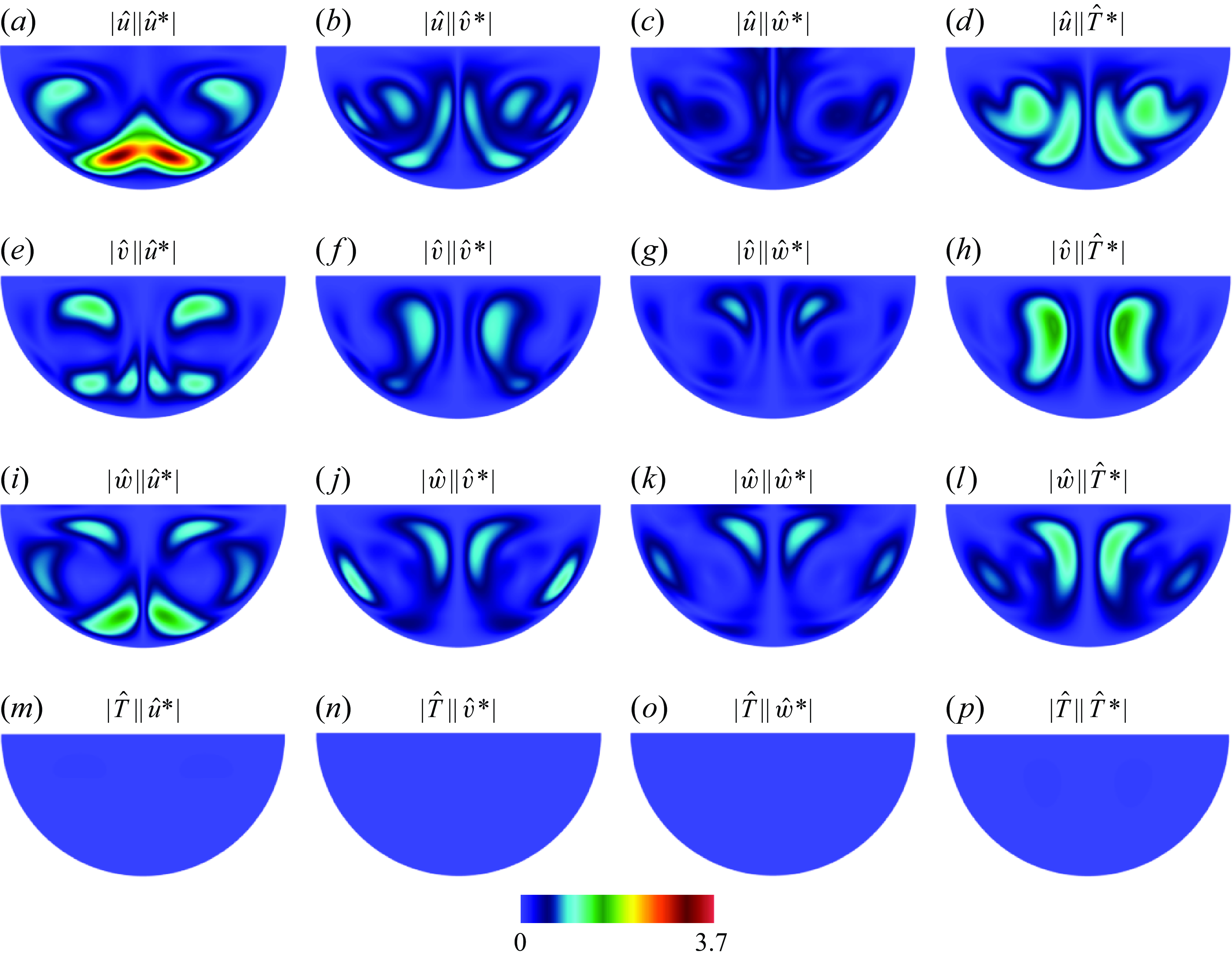
The absolute value of the components of the sensitivity tensor $S_{ij} = \hat {\textbf {q}}_i \hat {\textbf {q}}_j^*$
for the simulation case C2 (
$S_{ij} = \hat {\textbf {q}}_i \hat {\textbf {q}}_j^*$
for the simulation case C2 ( $Re=50$
,
$Re=50$
, $Ra=7 \times 10^3$
and
$Ra=7 \times 10^3$
and $k=6$
) in the
$k=6$
) in the $x{-}y$
plane.
$x{-}y$
plane.
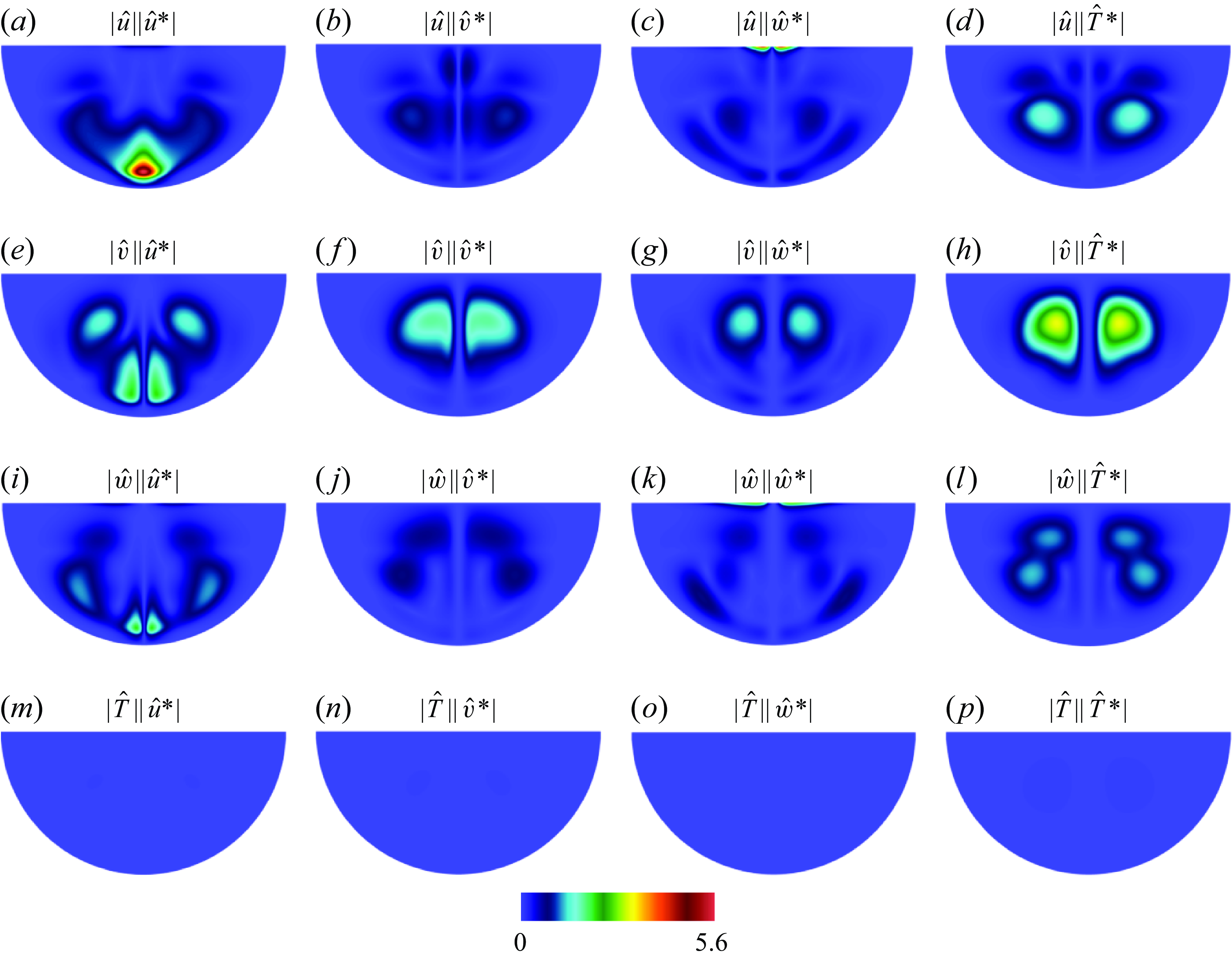
The absolute value of the components of the sensitivity tensor $S_{ij} = \hat {\textbf {q}}_i \hat {\textbf {q}}_j^*$
for the simulation case C3 (
$S_{ij} = \hat {\textbf {q}}_i \hat {\textbf {q}}_j^*$
for the simulation case C3 ( $Re=100$
,
$Re=100$
, $Ra=4 \times 10^4$
and
$Ra=4 \times 10^4$
and $k=4$
) in the
$k=4$
) in the $x{-}y$
plane.
$x{-}y$
plane.
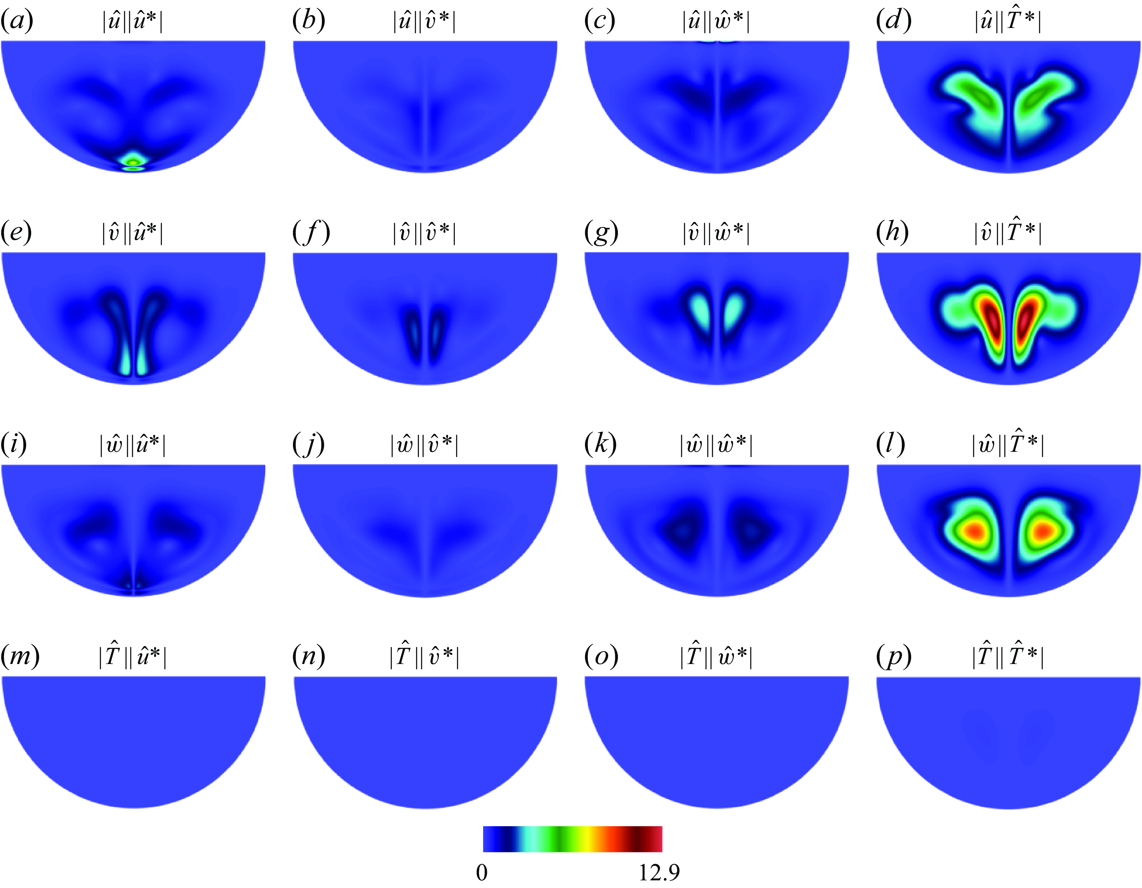
The absolute value of the components of the sensitivity tensor $S_{ij} = \hat {\textbf {q}}_i \hat {\textbf {q}}_j^*$
for the simulation case C4 (
$S_{ij} = \hat {\textbf {q}}_i \hat {\textbf {q}}_j^*$
for the simulation case C4 ( $Re=150$
,
$Re=150$
, $Ra=8 \times 10^4$
and
$Ra=8 \times 10^4$
and $k=6$
) in the
$k=6$
) in the $x{-}y$
plane.
$x{-}y$
plane.
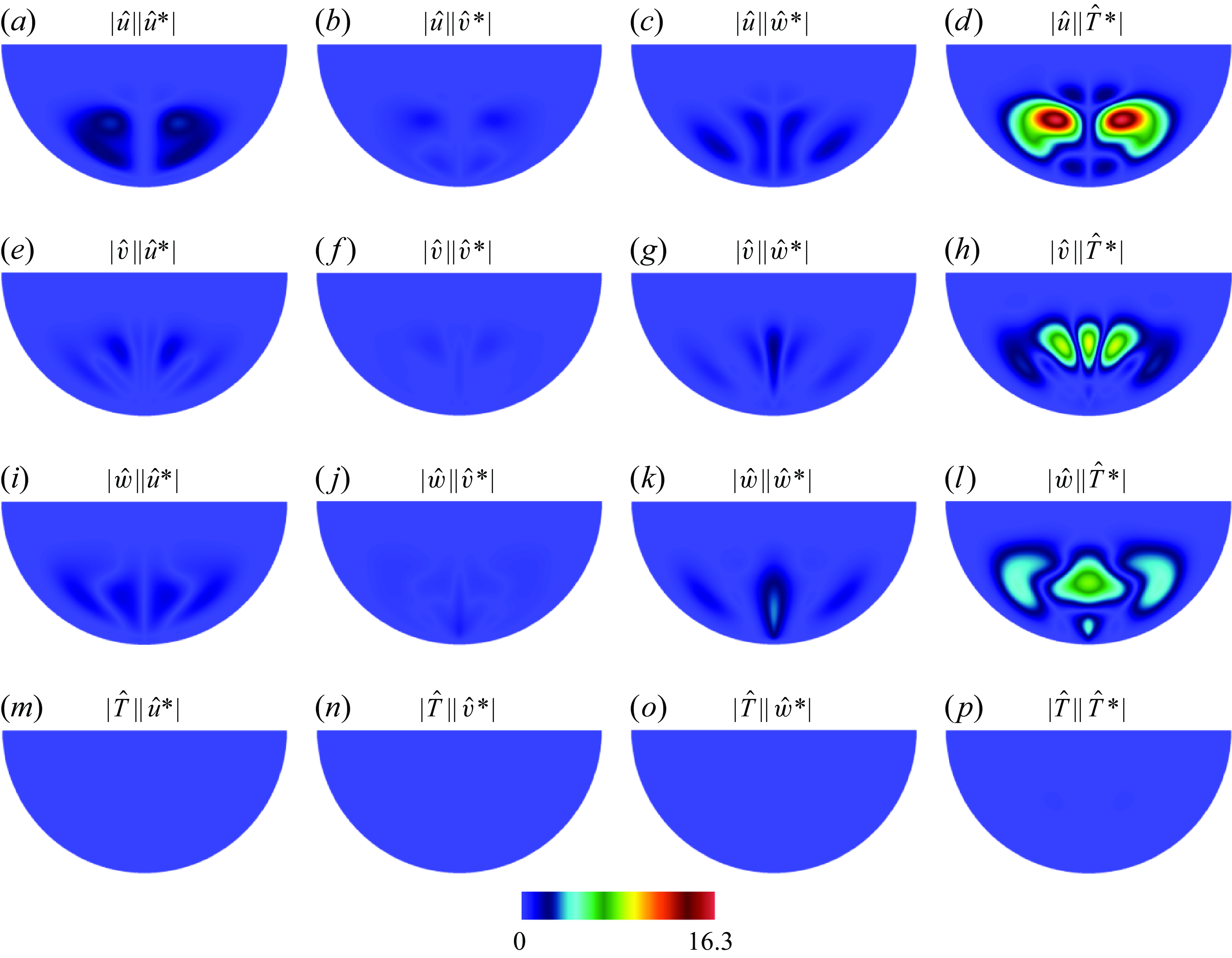
Crucially, these results applied to all four cases, regardless of whether the unstable mode is oscillatory or not, and whether it arises through a supercritical or a subcritical bifurcation. These results open interesting perspectives in view of the suppression of the instability. A possible strategy would consist in applying a mechanical actuation in the inflow region based on the receptivity map of the unstable mode, with amplitude and phase chosen to optimise the suppression of the optimal mode, through the linear evolution equations. Actuation should then be applied from the point where the unstable mode reaches a small, arbitrary threshold amplitude, until time $t_f$
. For
$t_f$
. For $t\gt t_f$
, the flow should be left to evolve until the unstable mode regains its initial threshold amplitude, at
$t\gt t_f$
, the flow should be left to evolve until the unstable mode regains its initial threshold amplitude, at $t=\eta _a t_f$
, at which point the actuation should be applied again, iterating the procedure for as long as the flow needs to be stabilised. The success of this strategy relies on the assumption that the threshold amplitude is sufficiently small for the unstable mode to evolve according to the linear equations. In other words, the strategy consists in preventing it from entering a nonlinear regime where the actuation would become ineffective.
$t=\eta _a t_f$
, at which point the actuation should be applied again, iterating the procedure for as long as the flow needs to be stabilised. The success of this strategy relies on the assumption that the threshold amplitude is sufficiently small for the unstable mode to evolve according to the linear equations. In other words, the strategy consists in preventing it from entering a nonlinear regime where the actuation would become ineffective.
The application of this idea raises a number of questions for further studies. First, we considered only a single unstable mode (or at most two). While similar restrictions apply to stabilisation techniques based on the properties of the adjoint equations, it is unclear how far beyond criticality this method would remain effective. Certainly, the cases studied in this paper showed that it remained effective even when more than one mode from the same branch was unstable (as in case C2). Another novel aspect of the mixed-convective problem we considered here, compared with the classical cylinder wake problem, is that in more supercritical flows, several branches of instabilities with different underlying mechanisms may become unstable. Since, however, the approach is linear, a linear combination of optimal actuations for each of the unstable modes may succeed in stabilising all of them, provided transient growth due to their possible non-orthogonality does not lead to perturbation amplitudes capable of igniting nonlinearities (Schmid & Henningson Reference Schmid and Henningson2001). Such an approach may involve the stabilisation of modes from different branches if the flow becomes multimodal, as for example magnetoconvective flows do (Xu et al. Reference Xu, Horn and Aurnou2023). In case one of these modes is subcritical (as for case C3), there is an additional risk that an altogether different branch of instability may drive the transition, even below the critical Rayleigh number of the linear stability of the leading eigenmode. Nonlinear simulations in the subcritical regime have shown subcritical convection was not ignited by the simple addition of random noise (Kumar & Pothérat Reference Kumar and Pothérat2020). A similar phenomenon occurs in quasi-2-D shear flows (Camobreco et al. Reference Camobreco, Pothérat and Sheard2021, Reference Camobreco, Pothérat and Sheard2022), where it turns out that the subcritical transition is still controlled by the linearly unstable mode. If this is still the case, then a receptivity-based actuation would still be expected to be able to suppress instability in the subcritical regime.
Funding
Part of this research was funded by Constellium Technology Center (C-TEC). Our numerical simulations were performed on Zeus of Coventry University and the Sulis Tier 2 HPC platform hosted by the Scientific Computing Research Technology Platform at the University of Warwick. A.P. acknowledges support from EPSRC, under grant no. EP/X010937/1.
Declaration of interests
The authors report no conflict of interest.
Appendix A. Sensitivity tensor
We examine the sensitivity tensor $S_{ij}$
to determine how individual components of the temperature and velocity fields feedback on each other to drive the instability associated with the leading eigenmode.
$S_{ij}$
to determine how individual components of the temperature and velocity fields feedback on each other to drive the instability associated with the leading eigenmode.
The first noticeable feature is that in all four cases C1–C4 represented on figures 9 to 12, all elements of the tensor associated with $|\hat T|$
, are practically identically zero, including
$|\hat T|$
, are practically identically zero, including $|\hat T||\hat T^*|$
. This means that the temperature perturbation responds to feedback from none of the components, not even a thermal one. On the other hand components of the tensor involving a velocity component and
$|\hat T||\hat T^*|$
. This means that the temperature perturbation responds to feedback from none of the components, not even a thermal one. On the other hand components of the tensor involving a velocity component and $|\hat T^*|$
all show a strong response, so that the temperature field of the perturbation can likely be affected by changes in the velocity field. This can be understood in view of the low value of
$|\hat T^*|$
all show a strong response, so that the temperature field of the perturbation can likely be affected by changes in the velocity field. This can be understood in view of the low value of $Pr$
considered here (and for other liquid metals): even if mechanical feedback overcomes viscous forces to act on the velocity field, it would still need to act on a
$Pr$
considered here (and for other liquid metals): even if mechanical feedback overcomes viscous forces to act on the velocity field, it would still need to act on a ${O}(Pr)$
time scale to overcome thermal diffusion and affect the temperature field. This is because thermal diffusion (low
${O}(Pr)$
time scale to overcome thermal diffusion and affect the temperature field. This is because thermal diffusion (low $Pr$
) is too fast, preventing thermal feedback from contributing to instability. Consequently, at low
$Pr$
) is too fast, preventing thermal feedback from contributing to instability. Consequently, at low $Pr$
, the instability relies on feedback through its velocity field, i.e. mechanical.
$Pr$
, the instability relies on feedback through its velocity field, i.e. mechanical.
In case C1, figure 9(a) highlights that the greatest feedback is received by $x$
-component of the velocity from the perturbation, from the
$x$
-component of the velocity from the perturbation, from the $x$
-velocity component of the actuation. The maximum coincides with the lower part of the flow domain where the baroclinic jets turns up, just upstream of the point where they meet each other, and where the instability starts. Case C2 also features maximum feedback from
$x$
-velocity component of the actuation. The maximum coincides with the lower part of the flow domain where the baroclinic jets turns up, just upstream of the point where they meet each other, and where the instability starts. Case C2 also features maximum feedback from $\hat u_x^*$
onto
$\hat u_x^*$
onto $\hat u_x$
. This time, however, the sensitivity area is localised right at the bottom of the domain, at the point where the instability is maximum in velocity amplitude. Cases C3 and C4, by contrast, exhibit the greatest response to a temperature feedback. All three components show high response in both cases. In case C3, the maximum receptivity is on the
$\hat u_x$
. This time, however, the sensitivity area is localised right at the bottom of the domain, at the point where the instability is maximum in velocity amplitude. Cases C3 and C4, by contrast, exhibit the greatest response to a temperature feedback. All three components show high response in both cases. In case C3, the maximum receptivity is on the $v$
component, but on the
$v$
component, but on the $u$
component for case C4.
$u$
component for case C4.


 Open access