



1. Introduction
Bubbly flows near walls are common phenomena in a wide range of applications, including ocean engineering (underwater vehicle, ship propulsion), chemical engineering (bubble columns, reactors) and energy production (heat exchangers, vapour generators). In these contexts, bubbles frequently appear in the vicinity of walls particularly in processes involving bow-wave breaking, cavitation, wall-boiling or jet impingement. The interaction between the bubbles and turbulent boundary layer induces substantial pressure fluctuations, which in turn generate significant hydrodynamic noise and structural vibration. These fluctuations can be expressed in terms of wavenumber–frequency spectra, potentially facilitating their incorporation into the integral formulation (Farassat Reference Farassat2007; Choi et al. Reference Choi, Hong, Song, Kwon, Park, Seol and Kim2021) when solving the Ffowcs Williams–Hawkings equation (Ffowcs Williams & Hawkings Reference Ffowcs Williams and Hawkings1969). The wavenumber–frequency spectrum for single-phase flows has been extensively investigated through early experimental and numerical studies (Willmarth & Wooldridge Reference Willmarth and Wooldridge1962; Kim, Moin & Moser Reference Kim, Moin and Moser1987; Choi & Moin Reference Choi and Moin1990). From a turbulence modelling point of view, the wavenumber–frequency spectrum fundamentally characterises the dynamic coupling between spatial and temporal scales of motion in turbulent flows (Wu & He Reference Wu and He2021). Establishing the wavenumber–frequency spectrum of wall-pressure fluctuations in bubbly flows is crucial for a deeper understanding of turbulent kinetic energy transfer and dissipation between the bubble and boundary layer interactions, and the subsequent acoustic predictions.
Experimental studies have provided valuable insights into the characteristics of wall-pressure fluctuations in single-phase flows and their corresponding wavenumber–frequency spectra. Willmarth & Wooldridge (Reference Willmarth and Wooldridge1962) conducted one of the earliest direct measurements of fluctuating wall pressure beneath a thick turbulent boundary layer, obtaining the mean-square pressure, the power spectrum and the space–time correlation of the pressure. The following experimental measurements endeavour to increase signal-to-noise ratio by using large arrays and small sensors (Blake & Chase Reference Blake and Chase1971; Abraham & Keith Reference Abraham and Keith1998; Hu Reference Hu2022) or by designing elaborate arrays such as a rotating disk (Prigent, Salze & Bailly Reference Prigent, Salze and Bailly2022) and a multi-pore Helmholtz resonator (Damani et al. Reference Damani, Butt, Torren, Devenport and Lowe2025), since extracting fluctuation data from strong background noise continues to be difficult (Haxter et al. Reference Haxter, Brouwer, Sesterhenn and Spehr2017). Experimental measurements of pressure fluctuation spectrum remain challenging due to the limitations in sensor size and spacing, constraining the capture of the spatio-temporal evolution of pressure fluctuation with a wide range.
Numerical simulations have complemented these efforts, thereby facilitating the exploration of wall-pressure spectra under controlled flow conditions. For single-phase turbulent channel flows, Choi & Moin (Reference Choi and Moin1990) obtained three-dimensional (3-D) wall-pressure spectrum using data from the direct numerical simulation (DNS) of a turbulent channel flow (Kim et al. Reference Kim, Moin and Moser1987) and identified the convective characteristic of wall-pressure fluctuations. At the same friction Reynolds number $\textit{Re}_\tau =180$
, Chang III et al. (Reference Chang, Piomelli and Blake1999), using a DNS database, localised the velocity field sources for the wall-pressure fluctuations, i.e. the buffer layer dominates the whole spectrum; the viscous layer and logarithmic region tend to contribute at high and low wavenumbers, respectively. With increasing Reynolds number, large-scale motions in the outer layer will affect the near-wall region (Abe, Kawammura & Choi Reference Abe, Kawammura and Choi2004), resulting in the increment of normalised mean-square wall pressure (Hu, Morfey & Sandham Reference Hu, Morfey and Sandham2006). To alleviate the high computational cost, large-eddy simulations (LES) have also been employed to investigate the pressure fluctuations in channel flows at high Reynolds numbers (Wilczek, Stevens & Meneveau Reference Wilczek, Stevens and Meneveau2015; Park & Moin Reference Park and Moin2016). By applying spectral proper orthogonal decomposition to the wall-pressure fluctuations at each wall-parallel plane, Anantharamu & Mahesh (Reference Anantharamu and Mahesh2020) proposed the potential to identify the contribution of large-scale coherent motion in the outer region at higher Reynolds numbers. Obtaining the 3-D wavenumber–frequency spectrum at high Reynolds numbers is not trivial owing to lengthy simulation times and substantial storage demands. Yang & Yang (Reference Yang and Yang2022) achieved the spectrum encompassing streamwise wavenumber, spanwise wavenumber and frequency at friction Reynolds numbers up to
$\textit{Re}_\tau =180$
, Chang III et al. (Reference Chang, Piomelli and Blake1999), using a DNS database, localised the velocity field sources for the wall-pressure fluctuations, i.e. the buffer layer dominates the whole spectrum; the viscous layer and logarithmic region tend to contribute at high and low wavenumbers, respectively. With increasing Reynolds number, large-scale motions in the outer layer will affect the near-wall region (Abe, Kawammura & Choi Reference Abe, Kawammura and Choi2004), resulting in the increment of normalised mean-square wall pressure (Hu, Morfey & Sandham Reference Hu, Morfey and Sandham2006). To alleviate the high computational cost, large-eddy simulations (LES) have also been employed to investigate the pressure fluctuations in channel flows at high Reynolds numbers (Wilczek, Stevens & Meneveau Reference Wilczek, Stevens and Meneveau2015; Park & Moin Reference Park and Moin2016). By applying spectral proper orthogonal decomposition to the wall-pressure fluctuations at each wall-parallel plane, Anantharamu & Mahesh (Reference Anantharamu and Mahesh2020) proposed the potential to identify the contribution of large-scale coherent motion in the outer region at higher Reynolds numbers. Obtaining the 3-D wavenumber–frequency spectrum at high Reynolds numbers is not trivial owing to lengthy simulation times and substantial storage demands. Yang & Yang (Reference Yang and Yang2022) achieved the spectrum encompassing streamwise wavenumber, spanwise wavenumber and frequency at friction Reynolds numbers up to $\textit{Re}_\tau \approx 1000$
. The 3-D spectrum facilitates the identification of cross-spectral characteristics in the subconvective region, which is otherwise smeared out in one- and two-dimensional (1-D and 2-D) spectra. In addition to the convective peak associated with the hydrodynamic component, the wall-pressure spectrum also reveals information about the acoustic component, which is prone to coupling with structural modes, despite its smaller magnitude. The acquisition of this subconvective peak requires compressible numerical simulation (Liu, Wang & Wang Reference Liu, Wang and Wang2024). When channel flows are laden with bubbles, the wall-pressure spectrum is expected to exhibit greater complexity, as the presence of bubbles modifies the turbulent flow characteristics within the channel.
$\textit{Re}_\tau \approx 1000$
. The 3-D spectrum facilitates the identification of cross-spectral characteristics in the subconvective region, which is otherwise smeared out in one- and two-dimensional (1-D and 2-D) spectra. In addition to the convective peak associated with the hydrodynamic component, the wall-pressure spectrum also reveals information about the acoustic component, which is prone to coupling with structural modes, despite its smaller magnitude. The acquisition of this subconvective peak requires compressible numerical simulation (Liu, Wang & Wang Reference Liu, Wang and Wang2024). When channel flows are laden with bubbles, the wall-pressure spectrum is expected to exhibit greater complexity, as the presence of bubbles modifies the turbulent flow characteristics within the channel.
Key parameters of previous numerical simulations of bubbly channel flow. Here $L_x \times L_y \times L_z$
denotes the computational domain size in the streamwise, wall-normal and spanwise directions, respectively;
$L_x \times L_y \times L_z$
denotes the computational domain size in the streamwise, wall-normal and spanwise directions, respectively; $\textit{Re}_\tau$
is the friction Reynolds number;
$\textit{Re}_\tau$
is the friction Reynolds number; $\rho _l / \rho _g$
and
$\rho _l / \rho _g$
and $\mu _l / \mu _g$
are the density and viscosity ratios of the liquid and gas phases, respectively – the short dash means that a physical ratio was used, but the value was not specified in the literature;
$\mu _l / \mu _g$
are the density and viscosity ratios of the liquid and gas phases, respectively – the short dash means that a physical ratio was used, but the value was not specified in the literature; $D_b / h$
is the bubble diameter normalised by the channel half-height;
$D_b / h$
is the bubble diameter normalised by the channel half-height; $D_b / \varDelta$
is the number of cells per bubble diameter in the representative case. The maximum mean gas volume fractions throughout the domain, denoted by
$D_b / \varDelta$
is the number of cells per bubble diameter in the representative case. The maximum mean gas volume fractions throughout the domain, denoted by $\overline {\alpha _{g}}$
, are listed.
$\overline {\alpha _{g}}$
, are listed.

Obtaining detailed flow information regarding the turbulent bubbly flows experimentally is challenging. Relying solely on pressure fluctuation measurements on the wall is insufficient to correlate wall-pressure fluctuations with the internal characteristics of turbulent bubbly flows. Such information can be achieved by numerical simulations. Over the past two decades, significant progress has been made in the study of bubbly channel flows, which are primarily focused on understanding the dynamic interaction between bubbles and turbulence, examining how bubbles influence flow properties such as the wall drag, turbulence intensity and mixing. Given the extensive existing literature, table 1 summarises several notable studies directly relevant to the present study, along with their key simulation parameters, including the computational domain size, the friction Reynolds number, the density and viscosity ratios of the liquid and gas phases, the ratios of bubble diameter to the channel half-height and to the cell size, and the maximum mean gas volume fraction throughout the domain.
Tryggvason and co-workers pioneered DNS of bubbly channel flows using a front-tracking method (Lu, Fernández & Tryggvason Reference Lu, Fernández and Tryggvason2005; Lu & Tryggvason Reference Lu and Tryggvason2006, Reference Lu and Tryggvason2007, Reference Lu and Tryggvason2008, Reference Lu and Tryggvason2013), enabling the detailed analysis of bubble–turbulence interactions. Their work demonstrated that deformable bubbles modify turbulence structures and wall drag (Lu et al. Reference Lu, Fernández and Tryggvason2005). Subsequent studies further clarified that bubble size influences velocity fluctuations, vorticity distributions and bubble spatial organisation across the channel (Lu & Tryggvason Reference Lu and Tryggvason2007, Reference Lu and Tryggvason2008), thereby altering the effective flow rate and viscous dissipation (Dabiri, Lu & Tryggvason Reference Dabiri, Lu and Tryggvason2013). At a higher friction Reynolds number ( $\textit{Re}_\tau = 250$
), Lu & Tryggvason (Reference Lu and Tryggvason2013) investigated the mechanism of specific bubbles motion, including bubble clusters and recirculation, raising the demands for studies under stronger turbulence.
$\textit{Re}_\tau = 250$
), Lu & Tryggvason (Reference Lu and Tryggvason2013) investigated the mechanism of specific bubbles motion, including bubble clusters and recirculation, raising the demands for studies under stronger turbulence.
Achieving high Reynolds numbers remains a key objective in studies of turbulent flows. As in single-phase turbulence, increasing the Reynolds number enlarges the scale separation between near-wall and outer motions, leading to a higher computational cost. The presence of bubbles further amplifies this complexity. It appears in table 1 that the friction Reynolds number is constrained to be smaller than 250. An exception is found in the cases calculated by Lakehal, Métrailler & Reboux (Reference Lakehal, Métrailler and Reboux2017), at $\textit{Re}_\tau =400$
, which represents the highest friction Reynolds number studied to date to the author’s knowledge. However, it was a specific LES case with bubbles attached to the wall and simulated for a short initial transient.
$\textit{Re}_\tau =400$
, which represents the highest friction Reynolds number studied to date to the author’s knowledge. However, it was a specific LES case with bubbles attached to the wall and simulated for a short initial transient.
A high-fidelity database of bubbly channel flows enables a detailed analysis of flow and bubble statistics, including the probability density function describing the bubble velocity and liquid kinetic energy spectra (Cifani, Kuerten & Geurts Reference Cifani, Kuerten and Geurts2020), the coherent structure (Hasslberger et al. Reference Hasslberger, Cifani, Chakraborty and Klein2020), Reynolds stress closure and turbulence dissipation (Santarelli, Roussel & Fröhlich Reference Santarelli, Roussel and Fröhlich2016; Bois Reference Bois2017; Ma et al. Reference Ma, Santarelli, Ziegenhein, Lucas and Fröhlich2017; du Cluzeau, Bois & Toutant Reference du Cluzeau, Bois and Toutant2019; Feng et al. Reference Feng, Yang, Mao, Lu and Tryggvason2019; Ma et al. Reference Ma, Lucas, Jakirlić and Fröhlich2020; Klein, Trummler & Radtke Reference Klein, Trummler and Radtke2022; Zhang et al. Reference Zhang, Liu, Wang, Yang and Chu2024). These studies motivate the identification of universal features with the potential to advance multiphase turbulence modelling of near-wall flows, in complement with homogeneous isotropic turbulence and pseudo-turbulence.
Another challenge for the high-fidelity simulation of bubbly turbulent flows arises from the large density and viscosity ratios between liquid and gas phases, which render the problem numerically stiff. To ensure numerical stability, many studies reduced density ratios to $\textit {O}(10)$
and viscosity ratios to
$\textit {O}(10)$
and viscosity ratios to $\textit {O}(1{\sim} 10)$
(see table 1), while only a few employ realistic parameters for air and water (Bolotnov et al. Reference Bolotnov, Jansen, Drew, Oberai, Lahey and Podowski2011; Santarelli & Fröehlich Reference Santarelli and Fröehlich2015, Reference Santarelli and Fröehlich2016; Santarelli et al. Reference Santarelli, Roussel and Fröhlich2016). The density and viscosity ratios significantly influence the wake intensity, buoyancy production in the turbulent kinetic energy budget, viscous dissipation and circulation within bubbles (Innocenti et al. Reference Innocenti, Jaccod, Popinet and Chibbaro2021; Mangani et al. Reference Mangani, Soligo, Roccon and Soldati2022; Lu, Yang & Deng Reference Lu, Yang and Deng2025). Therefore, using realistic density and viscosity parameters is preferable to better capture the underlying physics of the air–water system, especially for the analysis of pressure fluctuations.
$\textit {O}(1{\sim} 10)$
(see table 1), while only a few employ realistic parameters for air and water (Bolotnov et al. Reference Bolotnov, Jansen, Drew, Oberai, Lahey and Podowski2011; Santarelli & Fröehlich Reference Santarelli and Fröehlich2015, Reference Santarelli and Fröehlich2016; Santarelli et al. Reference Santarelli, Roussel and Fröhlich2016). The density and viscosity ratios significantly influence the wake intensity, buoyancy production in the turbulent kinetic energy budget, viscous dissipation and circulation within bubbles (Innocenti et al. Reference Innocenti, Jaccod, Popinet and Chibbaro2021; Mangani et al. Reference Mangani, Soligo, Roccon and Soldati2022; Lu, Yang & Deng Reference Lu, Yang and Deng2025). Therefore, using realistic density and viscosity parameters is preferable to better capture the underlying physics of the air–water system, especially for the analysis of pressure fluctuations.
Pressure fluctuations have received limited attention compared with velocity statistics among the bubbly flow studies. There remains a dearth of information regarding the spatio-temporal characteristics of pressure fluctuation in bubbly channel flows. The lack of studies on the pressure fluctuations of bubbly channel flows likely stems from the combined complexity of the high-fidelity simulation of the pressure field and deformable bubbles. The resolution requirements for accurately predicting pressure fluctuations are more stringent than those for velocity predictions (Park & Moin Reference Park and Moin2016). The Poisson equation governing the pressure fluctuations in an incompressible flow (Pope Reference Pope2000) implies that the velocity at every point affects the pressure fluctuation from a global perspective. The presence of bubbles introduces additional density-variation terms, analogous to the compressible component associated with compressibility effects (Sarkar Reference Sarkar1992; Lele Reference Lele1994; Livescu Reference Livescu2020), but more complex due to the sharp density gradient across bubble interfaces.
The purpose of the present study is therefore threefold. (i) To complement numerical simulation results of bubbly channel flows at the highest Reynolds number ever achieved, as far as we are aware, under comparable high gas volume fractions and with large density and viscosity ratios for water and air. (ii) To elucidate the respective contributions of different source terms in the Poisson equation of pressure fluctuations in various regions across the turbulent boundary layer. (iii) To reveal the spatio-temporal characteristics of bubble-induced wall-pressure fluctuations through wavenumber–frequency spectra. This study aims to provide a novel perspective on the interaction between bubbles and the turbulent boundary layer.
The rest of the paper is organised as follows. In § 2 we describe the numerical method, detailing the governing equations and the set-up of the simulation cases. In § 3 we examine the fundamental flow characteristics of bubbly channel flows. Section 4 investigates the source terms of the Poisson equation for pressure fluctuations to explore their contributions arising from different flow mechanisms. Section 5 analyses the wavenumber–frequency spectra of wall-pressure fluctuations. Finally, the conclusions are summarised in § 6.
2. Numerical procedure
2.1. Governing equations
The flow field comprising water and air bubbles is treated as a one-fluid incompressible mixture. The volume-of-fluid (VOF) method is employed to capture the bubble interfaces. The governing equations in Cartesian coordinates for the liquid-phase volume fraction $\alpha _l$
, the mass and momentum conservation read
$\alpha _l$
, the mass and momentum conservation read
 \begin{equation} \frac {{\partial \alpha _l }}{{\partial t}} + {u_i}\frac {{\partial \alpha _l }}{{\partial {x_i}}} = 0, \end{equation}
 \begin{equation} \frac {{\partial {u_i}}}{{\partial {x_i}}} = 0, \end{equation}
 \begin{equation} \frac {{\partial ({\rho _m}{u_i}})}{{\partial t}} + \frac {{\partial \left ( {{\rho _m}{u_i}{u_{\!j}}} \right )}}{{\partial {x_{\!j}}}} = - \frac {{\partial p}}{{\partial {x_i}}} + \frac {\partial \tau _{ij}^{\textit{eff}}}{\partial x_{\!j}} + {F_i^\sigma } + {F_i^{\textit {rep}}}, \end{equation}
where $p$
is the pressure field,
$p$
is the pressure field, $u_i$
is the velocity vector and
$u_i$
is the velocity vector and $(u,v,w)$
denote the components of the velocity vector in the
$(u,v,w)$
denote the components of the velocity vector in the $x$
,
$x$
, $y$
and
$y$
and $z$
directions, respectively. Gravity is neglected in the present work to focus on the interaction between bubbles and the turbulent boundary layer. The effective stress tensor, including both the molecular and subgrid-scale (SGS) contributions, is modelled as
$z$
directions, respectively. Gravity is neglected in the present work to focus on the interaction between bubbles and the turbulent boundary layer. The effective stress tensor, including both the molecular and subgrid-scale (SGS) contributions, is modelled as
 \begin{equation} \tau _{ij}^{\textit{eff}} = \tau _{ij}+\tau _{ij}^{\textit {SGS}} = \left ( {\mu _m} + {\mu _t}\right ) \left ( \frac {\partial u_i}{\partial x_{\!j}}+ \frac {\partial u_{\!j}}{\partial x_i} \right )\!. \end{equation}
The mixture density and viscosity are calculated using a volume-fraction-weighted approach: $\rho _m=\alpha _l\rho _l+\alpha _g\rho _g$
and
$\rho _m=\alpha _l\rho _l+\alpha _g\rho _g$
and $\mu _m=\alpha _l\mu _l+\alpha _g\mu _g$
, with the subscripts
$\mu _m=\alpha _l\mu _l+\alpha _g\mu _g$
, with the subscripts $l$
and
$l$
and $g$
denoting the liquid and gas phases, respectively. The two-phase volume fraction satisfies
$g$
denoting the liquid and gas phases, respectively. The two-phase volume fraction satisfies $\alpha _l+\alpha _g=1$
. Considering the necessity to resolve both the bubbles and boundary layer in order to capture precise pressure fluctuations, we employ the wall-adapting local eddy-viscosity (WALE) LES (Nicoud & Ducros Reference Nicoud and Ducros1999) to relax the requirement for extremely fine meshes near the wall. Thus, the turbulent viscosity
$\alpha _l+\alpha _g=1$
. Considering the necessity to resolve both the bubbles and boundary layer in order to capture precise pressure fluctuations, we employ the wall-adapting local eddy-viscosity (WALE) LES (Nicoud & Ducros Reference Nicoud and Ducros1999) to relax the requirement for extremely fine meshes near the wall. Thus, the turbulent viscosity $\mu _t=\rho _m\nu _t$
is included in the momentum equation. A thorough validation is performed by comparing the single-phase results with DNS data for velocity statistics (Lee & Moser Reference Lee and Moser2015) and pressure fluctuations spectra (Yang & Yang Reference Yang and Yang2022), demonstrating the high fidelity of the present LES (see Appendix A). The influence of the WALE model on bubbly flows is assessed in Appendix B in terms of the distributions of turbulent viscosity and SGS stresses. The time- and space-averaged turbulent kinematic viscosity
$\mu _t=\rho _m\nu _t$
is included in the momentum equation. A thorough validation is performed by comparing the single-phase results with DNS data for velocity statistics (Lee & Moser Reference Lee and Moser2015) and pressure fluctuations spectra (Yang & Yang Reference Yang and Yang2022), demonstrating the high fidelity of the present LES (see Appendix A). The influence of the WALE model on bubbly flows is assessed in Appendix B in terms of the distributions of turbulent viscosity and SGS stresses. The time- and space-averaged turbulent kinematic viscosity $\langle \nu _t \rangle$
remains below
$\langle \nu _t \rangle$
remains below $0.08$
times the water kinematic viscosity, while the SGS stresses are at least three orders of magnitude smaller than the resolved Reynolds stresses throughout the channel. Furthermore, the second-order velocity moments and the wall-pressure spectra are in close agreement with the corresponding under-resolved DNS (uDNS) results obtained without the explicit SGS model. These results demonstrate that the contribution of the WALE model remains negligible under the present grid resolution and does not influence the principal conclusions of the study. Nevertheless, the LES framework is retained for future investigations at higher Reynolds numbers.
$0.08$
times the water kinematic viscosity, while the SGS stresses are at least three orders of magnitude smaller than the resolved Reynolds stresses throughout the channel. Furthermore, the second-order velocity moments and the wall-pressure spectra are in close agreement with the corresponding under-resolved DNS (uDNS) results obtained without the explicit SGS model. These results demonstrate that the contribution of the WALE model remains negligible under the present grid resolution and does not influence the principal conclusions of the study. Nevertheless, the LES framework is retained for future investigations at higher Reynolds numbers.
The surface tension is modelled using the continuum surface force model (Brackbill, Kothe & Zemach Reference Brackbill, Kothe and Zemach1992) as $F_i^\sigma =\sigma \kappa \partial \alpha _l/\partial x_i$
, where
$F_i^\sigma =\sigma \kappa \partial \alpha _l/\partial x_i$
, where $\sigma$
is the constant surface-tension coefficient,
$\sigma$
is the constant surface-tension coefficient, $\kappa =- \partial n_i/ \partial x_i$
is the curvature of the interface and
$\kappa =- \partial n_i/ \partial x_i$
is the curvature of the interface and $n_i=\boldsymbol{\nabla }\alpha / \left | \boldsymbol{\nabla }\alpha \right |$
is the unit normal vector of the interfaces. The VOF method is prone to spurious numerical coalescence between bubbles (Zhang, Ni & Magnaudet Reference Zhang, Ni and Magnaudet2021; Innocenti et al. Reference Innocenti, Jaccod, Popinet and Chibbaro2021), requiring an extremely high grid resolution to prevent this unphysical phenomenon. An alternative way is to apply a short-range repulsive force on the interface through calibrating the artificial coefficient (Zhang et al. Reference Zhang, Peng, Shao and Deng2022). Considering the trade-offs, we adopt the latter approach with the coefficient
$n_i=\boldsymbol{\nabla }\alpha / \left | \boldsymbol{\nabla }\alpha \right |$
is the unit normal vector of the interfaces. The VOF method is prone to spurious numerical coalescence between bubbles (Zhang, Ni & Magnaudet Reference Zhang, Ni and Magnaudet2021; Innocenti et al. Reference Innocenti, Jaccod, Popinet and Chibbaro2021), requiring an extremely high grid resolution to prevent this unphysical phenomenon. An alternative way is to apply a short-range repulsive force on the interface through calibrating the artificial coefficient (Zhang et al. Reference Zhang, Peng, Shao and Deng2022). Considering the trade-offs, we adopt the latter approach with the coefficient $K=1\times 10^{-8}\,\textrm {J}$
to prevent unphysical bubble coalescence while avoiding excessive influence on the overall bubble motion. The repulsive force
$K=1\times 10^{-8}\,\textrm {J}$
to prevent unphysical bubble coalescence while avoiding excessive influence on the overall bubble motion. The repulsive force $F_i^{\textit{rep}}$
is incorporated into the source term of the momentum equation (2.3).
$F_i^{\textit{rep}}$
is incorporated into the source term of the momentum equation (2.3).
The simulations are performed using the open-source code OpenFOAM, employing the two-phase solver interFoam. The governing equations are discretised using the finite-volume method. Time advancement is performed with a first-order implicit Euler scheme. The divergence terms are evaluated using the Gauss theorem, which converts the cell-volume integrals into summations of face fluxes. The fluxes and the field quantities required at cell faces are obtained using second-order linear interpolation. For the phase-fraction equation, the advective flux is discretised using the second-order bounded van Leer scheme. An artificial compression term is introduced in the phase-fraction equation to counteract numerical diffusion of the interface; the corresponding compression flux is evaluated using second-order linear interpolation. The momentum convection term is discretised using a bounded flux-limited linear scheme, which retains second-order accuracy in smooth regions and locally reverts towards upwind differencing near steep gradients to improve boundedness and stability. The viscous stress divergence is also evaluated from face-flux summations, with the relevant quantities at cell faces obtained using second-order linear interpolation.
2.2. Computational set-up
The channel consists of two no-slip walls perpendicular to the direction $y$
and periodic boundaries in the streamwise
$y$
and periodic boundaries in the streamwise $x$
and spanwise
$x$
and spanwise $z$
directions. The computational domain is defined as
$z$
directions. The computational domain is defined as $L_x \times L_y \times L_z = 4h \times 2h \times 2h$
, where
$L_x \times L_y \times L_z = 4h \times 2h \times 2h$
, where $h$
is the channel half-height. This domain size is slightly larger than the ‘minimum turbulent channel‘ (
$h$
is the channel half-height. This domain size is slightly larger than the ‘minimum turbulent channel‘ ( $\pi h \times 2h \times \pi h/2$
) in Lu et al. (Reference Lu, Fernández and Tryggvason2005). Extending the channel configuration can facilitate the discovery of large-scale flow structures (Santarelli & Fröehlich Reference Santarelli and Fröehlich2015; Cifani, Kuerten & Geurts Reference Cifani, Kuerten and Geurts2018; Nemati et al. Reference Nemati, Breugem, Kwakkel and Boersma2021). However, the large computational domain appears formidable in the present simulation. In Appendix C we calculate the two-point correlation function in space, near the wall and at the channel centre, respectively, to validate the computational domain size. The computational domain is discretised with a structured mesh. Bubbles with diameters of
$\pi h \times 2h \times \pi h/2$
) in Lu et al. (Reference Lu, Fernández and Tryggvason2005). Extending the channel configuration can facilitate the discovery of large-scale flow structures (Santarelli & Fröehlich Reference Santarelli and Fröehlich2015; Cifani, Kuerten & Geurts Reference Cifani, Kuerten and Geurts2018; Nemati et al. Reference Nemati, Breugem, Kwakkel and Boersma2021). However, the large computational domain appears formidable in the present simulation. In Appendix C we calculate the two-point correlation function in space, near the wall and at the channel centre, respectively, to validate the computational domain size. The computational domain is discretised with a structured mesh. Bubbles with diameters of $D_b=2$
and 3 mm are considered in this study. From the grid-convergence analysis (see Appendix D), it is found that 30 grid cells per bubble diameter are sufficient to achieve convergence in the distribution of the gas volume fraction, velocity profiles and second-order velocity moments. The channel half-height is set to
$D_b=2$
and 3 mm are considered in this study. From the grid-convergence analysis (see Appendix D), it is found that 30 grid cells per bubble diameter are sufficient to achieve convergence in the distribution of the gas volume fraction, velocity profiles and second-order velocity moments. The channel half-height is set to $h=0.01$
m, resulting in the ratio
$h=0.01$
m, resulting in the ratio $D_b/h = 0.2$
and 0.3. For
$D_b/h = 0.2$
and 0.3. For $D_b=2$
mm, the computational domain is meshed with
$D_b=2$
mm, the computational domain is meshed with $N_x \times N_y \times N_z = 600 \times 400 \times 300$
, corresponding to a wall-unit resolution of
$N_x \times N_y \times N_z = 600 \times 400 \times 300$
, corresponding to a wall-unit resolution of $\varDelta x^+ = \varDelta z^+ = 3.67$
in the streamwise and spanwise directions. The grid employs a uniform expansion rate in the wall-normal
$\varDelta x^+ = \varDelta z^+ = 3.67$
in the streamwise and spanwise directions. The grid employs a uniform expansion rate in the wall-normal $y$
direction to enhance near-wall resolution, resulting in
$y$
direction to enhance near-wall resolution, resulting in $\varDelta y^+ |_{y=0}= \varDelta y^+ |_{y=2h}=1.85$
and
$\varDelta y^+ |_{y=0}= \varDelta y^+ |_{y=2h}=1.85$
and $\varDelta y^+|_{y=h}/ \varDelta y^+ |_{y=0}= 2.1$
. For
$\varDelta y^+|_{y=h}/ \varDelta y^+ |_{y=0}= 2.1$
. For $D_b=3$
mm, the numbers of the mesh are
$D_b=3$
mm, the numbers of the mesh are $N_x \times N_y \times N_z = 400 \times 300 \times 200$
with resolution
$N_x \times N_y \times N_z = 400 \times 300 \times 200$
with resolution $\varDelta x^+ = \varDelta z^+ = 5.5$
,
$\varDelta x^+ = \varDelta z^+ = 5.5$
, $\varDelta y^+ |_{y=0}= \varDelta y^+ |_{y=2h}=1.47$
and
$\varDelta y^+ |_{y=0}= \varDelta y^+ |_{y=2h}=1.47$
and $\varDelta y^+|_{y=h}/ \varDelta y^+ |_{y=0}= 5$
. These details of the mesh configurations and parameters of cases are listed in table 2. The number 64 or 128 in the case name denotes the bubble count and ‘D2’ or ‘D3’ denotes the bubble diameter. In this paper, the superscript ’+’ denotes variables normalised using wall units, i.e. viscous length
$\varDelta y^+|_{y=h}/ \varDelta y^+ |_{y=0}= 5$
. These details of the mesh configurations and parameters of cases are listed in table 2. The number 64 or 128 in the case name denotes the bubble count and ‘D2’ or ‘D3’ denotes the bubble diameter. In this paper, the superscript ’+’ denotes variables normalised using wall units, i.e. viscous length $\delta _\nu =\nu _l /u_\tau$
and wall-friction velocity
$\delta _\nu =\nu _l /u_\tau$
and wall-friction velocity $u_\tau$
as the characteristic length and velocity scales, respectively, where
$u_\tau$
as the characteristic length and velocity scales, respectively, where $\nu _l=\mu _l/\rho _l$
is the kinematic viscosity of the liquid and
$\nu _l=\mu _l/\rho _l$
is the kinematic viscosity of the liquid and $\mu _l$
is the dynamic viscosity of the liquid. The density and viscosity for water and air under standard atmospheric pressure and at 20
$\mu _l$
is the dynamic viscosity of the liquid. The density and viscosity for water and air under standard atmospheric pressure and at 20 $^\circ$
C are employed, i.e.
$^\circ$
C are employed, i.e. $\rho _l=998.18\,{\textrm {kg}\,{\textrm {m}}^{-3}}$
,
$\rho _l=998.18\,{\textrm {kg}\,{\textrm {m}}^{-3}}$
, $\nu _l = 1.00\times 10^{-6}\,{\textrm {m}^2\textrm {s}^{-1}}$
,
$\nu _l = 1.00\times 10^{-6}\,{\textrm {m}^2\textrm {s}^{-1}}$
, $\rho _g=1.1881\, {\textrm {kg}\,{\textrm {m}}^{-3}}$
and
$\rho _g=1.1881\, {\textrm {kg}\,{\textrm {m}}^{-3}}$
and $\nu _g = 1.83\times 10^{-5}\,{\textrm {m}^2\textrm {s}^{-1}}$
. Naturally, the interfacial tension between the gas and liquid phases adopts the standard value at ambient temperature, i.e.
$\nu _g = 1.83\times 10^{-5}\,{\textrm {m}^2\textrm {s}^{-1}}$
. Naturally, the interfacial tension between the gas and liquid phases adopts the standard value at ambient temperature, i.e. $\sigma = 0.072\,{\textrm {N m}^{-1}}$
.
$\sigma = 0.072\,{\textrm {N m}^{-1}}$
.
Simulation parameters for all cases. The channel half-height is $h = 0.01$
m. The mesh for case B128D2 is identical to that for B64D2, and the mesh for B128D3 is identical to that for B64D3.
$h = 0.01$
m. The mesh for case B128D2 is identical to that for B64D2, and the mesh for B128D3 is identical to that for B64D3.

During the simulations, the Courant–Friedrichs–Lewy number is maintained at 0.5. The interfacial Courant number, which is defined based on the volumetric flux magnitude in the vicinity of the interface and provides a measure of the local interface advection speed relative to the cell size, is also restricted to 0.5 for all bubbly cases. In addition, surface-tension resolution is assessed using the cell-surface Weber number $We_\varDelta = \rho _l u_{\textit{rms}}^2 \varDelta / 4\pi \sigma$
(Popinet Reference Popinet2018). In the present work,
$We_\varDelta = \rho _l u_{\textit{rms}}^2 \varDelta / 4\pi \sigma$
(Popinet Reference Popinet2018). In the present work, $We_\varDelta \lt 0.001$
, ensuring surface-tension forces are well resolved.
$We_\varDelta \lt 0.001$
, ensuring surface-tension forces are well resolved.
Since the instantaneous turbulent flow fields, especially in bubbly cases, are not perfectly symmetric up and down, the wall shear stress $\tau _w$
is computed based on the streamwise velocity profile and averaged with the values at the bottom and top walls, i.e.
$\tau _w$
is computed based on the streamwise velocity profile and averaged with the values at the bottom and top walls, i.e.
 \begin{equation} {\tau _w} = \frac {{{{\left . {{\tau _w}} \right |}_{y = 0}} + {{\left . {{\tau _w}} \right |}_{y = 2h}}}}{2} = \frac {1}{2}\left ( {{{\left . {{\mu _l}\frac {{{\mathrm{d}}\left \langle u \right \rangle }}{{{\mathrm{d}}y}}} \right |}_{y = 0}} - {{\left . {{\mu _l}\frac {{{\mathrm{d}}\left \langle u \right \rangle }}{{{\mathrm{d}}y}}} \right |}_{y = 2h}}} \right )\!, \end{equation}
and the wall-friction velocity $u_\tau$
is calculated based on the above wall shear stress as
$u_\tau$
is calculated based on the above wall shear stress as
 \begin{equation} {u_\tau } = \sqrt {\frac {{{\tau _w}}}{{{\rho _l}}}}. \end{equation}
The friction Reynolds number is calculated by $R{e_\tau } = {{u_\tau }h}/{{\nu _l}}$
. The pair of angular brackets in (2.5) denotes averaging over time and the streamwise–spanwise plane, i.e.
$R{e_\tau } = {{u_\tau }h}/{{\nu _l}}$
. The pair of angular brackets in (2.5) denotes averaging over time and the streamwise–spanwise plane, i.e.
 \begin{equation} \left \langle \phi \right \rangle (y) = \frac {1}{{\varDelta {T}{L_x}{L_z}}}\int _t^{t + \varDelta {T}} {\int _0^{{L_x}} {\int _0^{{L_z}} {\phi \left ( {x,y,z,t} \right ){\mathrm{d}}z{\mathrm{d}}x{\mathrm{d}}t} } }, \end{equation}
where $\varDelta T$
is the sampling period. The averaging in (2.7) results in a function that varies only with the
$\varDelta T$
is the sampling period. The averaging in (2.7) results in a function that varies only with the $y$
coordinate.
$y$
coordinate.
To facilitate the subsequent discussion, we introduce the decomposition of the field into the mean and fluctuation components from the perspective of Reynolds decomposition. A field $\phi (x,y,z)$
can thus be expressed as
$\phi (x,y,z)$
can thus be expressed as
 \begin{equation} \phi (x,y,z,t) = \overline {\phi }(x,y,z) + \phi '(x,y,z,t), \end{equation}
where the overbar denotes time averaging applied to the mixture field (i.e. without phase discrimination) and the prime denotes the corresponding fluctuation about this mixture-averaged mean. It should be noted that this approach differs from the phase-averaged decomposition employed in some studies listed in table 1 (e.g. Bolotnov et al. (Reference Bolotnov, Jansen, Drew, Oberai, Lahey and Podowski2011), Lakehal et al. (Reference Lakehal, Métrailler and Reboux2017), Cifani et al. (Reference Cifani, Kuerten and Geurts2018), du Cluzeau et al. (Reference du Cluzeau, Bois and Toutant2019), Cifani et al. (Reference Cifani, Kuerten and Geurts2020), Trautner et al. (Reference Trautner, Klein, Bräuer and Hasslberger2021)); consequently, the resulting fluctuations $\phi ^\prime$
contain contributions from both turbulent motions and interfacial dynamics.
$\phi ^\prime$
contain contributions from both turbulent motions and interfacial dynamics.
Channel flow must be driven by a streamwise pressure gradient to balance the shear stress. Some studies employed a fixed pressure gradient (Lu & Tryggvason Reference Lu and Tryggvason2006; Liu et al. Reference Liu, Wang, Yang, Nemati and Chu2023), while others used temporally variable pressure gradients to maintain fixed parameters, such as the friction Reynolds number (du Cluzeau et al. Reference du Cluzeau, Bois and Toutant2019, Reference du Cluzeau, Bois, Toutant and Martinez2020), bulk velocity (Cifani et al. Reference Cifani, Kuerten and Geurts2020) or mass flux (Hasslberger et al. Reference Hasslberger, Cifani, Chakraborty and Klein2020; Klein et al. Reference Klein, Trummler and Radtke2022). In this paper, a fixed pressure gradient is applied for the single-phase channel case, while temporally variable pressure gradients are imposed for bubbly cases to ensure a consistent bulk velocity $U_b$
. Thus, the bulk Reynolds numbers
$U_b$
. Thus, the bulk Reynolds numbers $\textit{Re}_{_B} = 2h U_b /\nu _l$
are uniform for all cases.
$\textit{Re}_{_B} = 2h U_b /\nu _l$
are uniform for all cases.
A single-phase turbulent channel flow filled with water is first simulated under the friction Reynolds number $\textit{Re}_\tau =550$
. The velocity field is initialised using a Blasius profile with prescribed perturbations following De Villiers (Reference De Villiers2006) to accelerate the transition to a fully developed turbulent flow. Integrating
$\textit{Re}_\tau =550$
. The velocity field is initialised using a Blasius profile with prescribed perturbations following De Villiers (Reference De Villiers2006) to accelerate the transition to a fully developed turbulent flow. Integrating $ \left \langle u \right \rangle$
in the
$ \left \langle u \right \rangle$
in the $y$
direction yields the bulk mean velocity
$y$
direction yields the bulk mean velocity $U_b$
and the corresponding bulk Reynolds number is
$U_b$
and the corresponding bulk Reynolds number is $\textit{Re}_{_B} = 20\,700$
, which will be applied to the bubbly flows. Consequently, the friction Reynolds number will vary within a narrow range among different bubbly cases. After a transient period, the turbulence reaches a statistically stationary state, and the data are sampled over a duration of
$\textit{Re}_{_B} = 20\,700$
, which will be applied to the bubbly flows. Consequently, the friction Reynolds number will vary within a narrow range among different bubbly cases. After a transient period, the turbulence reaches a statistically stationary state, and the data are sampled over a duration of $30L_x/U_b$
for further time averaging and post-processing.
$30L_x/U_b$
for further time averaging and post-processing.
The instantaneous velocity field at the end of the single-phase channel flow simulation is used as the initial velocity field for the bubbly cases. The influence of the initial bubble positions has been examined. After release, the bubbles undergo significant deformation and subsequently migrate toward the channel centreline, largely independent of their initial release locations. To shorten the transient period and reduce the simulation time, spherical bubbles are initially introduced into the flow field near the channel core in all subsequent bubbly cases. After initialisation, each simulation is advanced for an additional $7.77\,L_x/U_b$
to ensure that the system reaches a statistically stationary state. Subsequently, data are collected over an averaging duration of
$7.77\,L_x/U_b$
to ensure that the system reaches a statistically stationary state. Subsequently, data are collected over an averaging duration of $38.86\,L_x/U_b$
. The statistical convergence with this averaging duration is examined in Appendix E, where the temporal stabilisation of first- and second-order quantities as well as the symmetry between the upper and lower halves of the channel are demonstrated.
$38.86\,L_x/U_b$
. The statistical convergence with this averaging duration is examined in Appendix E, where the temporal stabilisation of first- and second-order quantities as well as the symmetry between the upper and lower halves of the channel are demonstrated.
3. Bubble distribution and flow statistics of turbulent bubbly channel flows
In this section the bubble distribution and flow statistics in turbulent bubbly channel flows are analysed. Figure 1 illustrates a first qualitative impression of the bubble distributions within the channel for different cases. Bubbles mainly accumulate in the core of the channel. As the gas volume fraction increases, a growing number of bubbles are observed in the near-wall region. Visually, the contours of wall-pressure fluctuations exhibit structural features similar to those in single-phase flow, characterised by alternating regions of high and low pressure.
Snapshots of bubble distribution and wall-pressure fluctuations for cases (a) B64D2, (b) B128D2, (c) B64D3, and (d) B128D3. The walls are coloured by pressure fluctuations $p'$
.
$p'$
.

Figure 1. Long description
Panel A: A heat map showing bubble distribution and wall-pressure fluctuations for case B64D2. The walls are colored by pressure fluctuations, with a color scale ranging from -10 to 10. The x-axis and y-axis represent spatial dimensions, and the z-axis represents the pressure fluctuations. Bubbles are distributed sparsely, and the pressure fluctuations show a varied pattern. Panel B: A heat map showing bubble distribution and wall-pressure fluctuations for case B128D2. The walls are colored by pressure fluctuations, with a color scale ranging from -10 to 10. The x-axis and y-axis represent spatial dimensions, and the z-axis represents the pressure fluctuations. Bubbles are more densely packed compared to Panel A, and the pressure fluctuations show a more intense pattern. Panel C: A heat map showing bubble distribution and wall-pressure fluctuations for case B64D3. The walls are colored by pressure fluctuations, with a color scale ranging from -10 to 10. The x-axis and y-axis represent spatial dimensions, and the z-axis represents the pressure fluctuations. Bubbles are distributed moderately, and the pressure fluctuations show a mixed pattern. Panel D: A heat map showing bubble distribution and wall-pressure fluctuations for case B128D3. The walls are colored by pressure fluctuations, with a color scale ranging from -10 to 10. The x-axis and y-axis represent spatial dimensions, and the z-axis represents the pressure fluctuations. Bubbles are densely packed, and the pressure fluctuations show a highly intense pattern.
(a) Profile of spatio-temporally averaged dimensionless streamwise velocity $\langle u\rangle^+$
. The black dashed line represents the viscous sublayer profile
$\langle u\rangle^+$
. The black dashed line represents the viscous sublayer profile $u^+ = y^+$
and log-law profile
$u^+ = y^+$
and log-law profile $u^+=({1}/{\kappa })\ln y^+ + B$
with
$u^+=({1}/{\kappa })\ln y^+ + B$
with $\kappa =0.4$
and
$\kappa =0.4$
and $B=5.5$
. (b) Liquid velocity
$B=5.5$
. (b) Liquid velocity $\langle u_l \rangle = \langle \alpha _l \boldsymbol{\cdot }u \rangle /\langle \alpha \rangle$
(solid lines) and gas velocity
$\langle u_l \rangle = \langle \alpha _l \boldsymbol{\cdot }u \rangle /\langle \alpha \rangle$
(solid lines) and gas velocity $\langle u_g \rangle = \langle \alpha _g \boldsymbol{\cdot }u \rangle /\langle \alpha _g \rangle$
(dashed lines). (c) Deformation coefficients
$\langle u_g \rangle = \langle \alpha _g \boldsymbol{\cdot }u \rangle /\langle \alpha _g \rangle$
(dashed lines). (c) Deformation coefficients $\chi$
. (d) Average of gas volume fraction
$\chi$
. (d) Average of gas volume fraction $\langle \alpha _g \rangle$
. The curve colour denoting each case is consistent with that in (a).
$\langle \alpha _g \rangle$
. The curve colour denoting each case is consistent with that in (a).

Figure 2. Long description
Panel A: A line graph shows the profile of spatio-temporally averaged dimensionless streamwise velocity. The x-axis is labeled y+ and the y-axis is labeled <u>/u_tau. The black dashed line represents the viscous sublayer profile and log-law profile with specific parameters. Panel B: A line graph displays liquid velocity (solid lines) and gas velocity (dashed lines) with the x-axis labeled y/h and the y-axis labeled <u>/Ub. Panel C: A line graph illustrates deformation coefficients with the x-axis labeled y/h and the y-axis labeled <x>. Panel D: A line graph presents the average of gas volume fraction with the x-axis labeled y/h and the y-axis labeled <alpha_g>. The curve color denoting each case is consistent across all panels.
Figure 2(a) shows the spatio-temporally averaged streamwise velocity profiles for all cases. The velocity profiles of the bubbly flows closely resemble that of the single-phase case. In the logarithmic region, the values of $\left \langle u \right \rangle ^+$
in the bubbly flows are slightly higher than that in the single-phase flow, whereas the values in the viscous sublayer and the buffer layer remain nearly identical, indicating that the presence of bubbles does not modify the mean velocity characteristics of the near-wall turbulence.
$\left \langle u \right \rangle ^+$
in the bubbly flows are slightly higher than that in the single-phase flow, whereas the values in the viscous sublayer and the buffer layer remain nearly identical, indicating that the presence of bubbles does not modify the mean velocity characteristics of the near-wall turbulence.
The velocity distributions of both the gas and liquid phases are shown in figure 2(b). Under the present non-gravity conditions, the relative velocity between the phases is small. Following the approach of Bunner & Tryggvason (Reference Bunner and Tryggvason2003), bubble deformation is quantified by $\chi$
, defined as the square root of the ratio of the largest to the smallest eigenvalue of the second moment of the inertia tensor. As shown in figure 2(c), the values of
$\chi$
, defined as the square root of the ratio of the largest to the smallest eigenvalue of the second moment of the inertia tensor. As shown in figure 2(c), the values of $\chi$
remain close to unity in most regions of the channel, indicating that the bubbles maintain a nearly spherical shape, whereas deformations occur near the wall where
$\chi$
remain close to unity in most regions of the channel, indicating that the bubbles maintain a nearly spherical shape, whereas deformations occur near the wall where $\chi$
reach up to 1.2. Bubbles with
$\chi$
reach up to 1.2. Bubbles with $D_b=3$
mm exhibit greater deformation than those with
$D_b=3$
mm exhibit greater deformation than those with $D_b=2$
mm, as expected. Additionally, case B128D3 exhibits marginally higher deformation than B64D3, likely due to enhanced bubble interactions at a higher gas volume fraction.
$D_b=2$
mm, as expected. Additionally, case B128D3 exhibits marginally higher deformation than B64D3, likely due to enhanced bubble interactions at a higher gas volume fraction.
The profiles of spatio-temporally averaged volume of gas $\langle \alpha _g \rangle$
for the bubbly cases are shown in figure 2(d). Both core-peaking and near-wall-peaking bubble distributions are observed in the present numerical results. The locations of these peaks are closely related to the lift force acting on the bubbles. Given the limited deformation, the direction of the lift force is expected to align with classical Saffman models (Saffman Reference Saffman1965). The mean liquid velocity
$\langle \alpha _g \rangle$
for the bubbly cases are shown in figure 2(d). Both core-peaking and near-wall-peaking bubble distributions are observed in the present numerical results. The locations of these peaks are closely related to the lift force acting on the bubbles. Given the limited deformation, the direction of the lift force is expected to align with classical Saffman models (Saffman Reference Saffman1965). The mean liquid velocity $\left \langle u_l \right \rangle$
exhibits a convex profile, whereas the gas velocity
$\left \langle u_l \right \rangle$
exhibits a convex profile, whereas the gas velocity $\langle u_g \rangle$
in the core region is lower than that of the liquid. Consequently, in the bubble reference frame, the liquid on the side of the channel centre moves faster, generating a lift force directed toward the channel centre. This mechanism explains the accumulation of bubbles in the central region, as shown in figure 2(d). It also accounts for the observation that, in cases B64D2 and B128D2, as the number of bubbles increases, the peak of the gas volume fraction grows higher rather than broadening at a constant height. For an even higher gas volume fraction (case B128D3), the relative velocity between phases and the distribution of the gas volume fraction become more intricate. In case B128D3, within the ranges
$\langle u_g \rangle$
in the core region is lower than that of the liquid. Consequently, in the bubble reference frame, the liquid on the side of the channel centre moves faster, generating a lift force directed toward the channel centre. This mechanism explains the accumulation of bubbles in the central region, as shown in figure 2(d). It also accounts for the observation that, in cases B64D2 and B128D2, as the number of bubbles increases, the peak of the gas volume fraction grows higher rather than broadening at a constant height. For an even higher gas volume fraction (case B128D3), the relative velocity between phases and the distribution of the gas volume fraction become more intricate. In case B128D3, within the ranges $0.3\lt y/h\lt 0.7$
and
$0.3\lt y/h\lt 0.7$
and $1.3\lt y/h\lt 1.7$
,
$1.3\lt y/h\lt 1.7$
, $\langle u_g \rangle$
remains smaller than
$\langle u_g \rangle$
remains smaller than $\left \langle u_l \right \rangle$
, indicating that the lift force still acts toward the channel centre. However, in the outer region
$\left \langle u_l \right \rangle$
, indicating that the lift force still acts toward the channel centre. However, in the outer region $0.7\lt y/h\lt 1.3$
,
$0.7\lt y/h\lt 1.3$
, $\langle u_g \rangle$
becomes very close to, or even slightly exceeds
$\langle u_g \rangle$
becomes very close to, or even slightly exceeds $\left \langle u_l \right \rangle$
, suggesting that the local gas volume fraction may approach a saturation state in this region. In addition to this core accumulation, additional near-wall peaks in
$\left \langle u_l \right \rangle$
, suggesting that the local gas volume fraction may approach a saturation state in this region. In addition to this core accumulation, additional near-wall peaks in $\langle \alpha _g \rangle$
appear at approximately
$\langle \alpha _g \rangle$
appear at approximately $y/h = 0.3$
and 1.7. A similar accumulation at the edge of the core region was found experimentally (Kashinsky & Randin Reference Kashinsky and Randin1999), occurring at relatively high gas volume fractions (above 16 %), and was also reported in the numerical simulations by Lu & Tryggvason (Reference Lu and Tryggvason2006) with a global gas volume fraction of 6 %. The near-wall peaks may result from a combined effect of transverse force balance and spatial confinement within the channel core.
$y/h = 0.3$
and 1.7. A similar accumulation at the edge of the core region was found experimentally (Kashinsky & Randin Reference Kashinsky and Randin1999), occurring at relatively high gas volume fractions (above 16 %), and was also reported in the numerical simulations by Lu & Tryggvason (Reference Lu and Tryggvason2006) with a global gas volume fraction of 6 %. The near-wall peaks may result from a combined effect of transverse force balance and spatial confinement within the channel core.
Profiles of the second-order velocity moments for bubbly and single-phase cases: (a) shear component, (b) streamwise component, (c) wall-normal component, and (d) spanwise component.

Figure 3. Long description
The image contains four line graphs labeled (a), (b), (c), and (d), each depicting profiles of second-order velocity moments for bubbly and single-phase cases. Panel A: The line graph shows the shear component of velocity moments. The x-axis is labeled y/h, and the y-axis is labeled with the dimensionless unit u_tau squared. Multiple lines represent different cases, including B64D2, B128D2, B64D3, B128D3, and SP. The lines show varying trends, with some peaking and others dipping. Panel B: The line graph shows the streamwise component of velocity moments. The x-axis is labeled y/h, and the y-axis is labeled with the dimensionless unit u_tau squared. Multiple lines represent different cases, including B64D2, B128D2, B64D3, B128D3, and SP. The lines show a general trend of decreasing values with some peaks near the edges. Panel C: The line graph shows the wall-normal component of velocity moments. The x-axis is labeled y/h, and the y-axis is labeled with the dimensionless unit u_tau squared. Multiple lines represent different cases, including B64D2, B128D2, B64D3, B128D3, and SP. The lines show varying trends with multiple peaks and valleys. Panel D: The line graph shows the spanwise component of velocity moments. The x-axis is labeled y/h, and the y-axis is labeled with the dimensionless unit u_tau squared. Multiple lines represent different cases, including B64D2, B128D2, B64D3, B128D3, and SP. The lines show varying trends with peaks and valleys.
Ratio of each second-order velocity moment: solid lines represent $\langle u^\prime u^\prime \rangle / k$
, dashed lines represent
$\langle u^\prime u^\prime \rangle / k$
, dashed lines represent $\langle v^\prime v^\prime \rangle / k$
and dotted lines represent
$\langle v^\prime v^\prime \rangle / k$
and dotted lines represent $\langle w^\prime w^\prime \rangle / k$
.
$\langle w^\prime w^\prime \rangle / k$
.

Figure 3 shows the distributions of the second-order velocity moments for both the bubbly and single-phase cases. The shear component $-\langle u^\prime v^\prime \rangle$
(figure 3
a) shows no significant difference between the bubbly and single-phase cases, although the bubbly cases exhibit a slightly imperfect linear slope. This behaviour arises from the balance between the total shear stress and the mean pressure gradient, which may be perturbed by the presence of bubbles. On the other hand, noticeable deviations from the single-phase case appear in the streamwise, wall-normal and spanwise components (figure 3
b–d), where regions with higher gas volume fractions exhibit enhanced turbulence intensities. In particular,
$-\langle u^\prime v^\prime \rangle$
(figure 3
a) shows no significant difference between the bubbly and single-phase cases, although the bubbly cases exhibit a slightly imperfect linear slope. This behaviour arises from the balance between the total shear stress and the mean pressure gradient, which may be perturbed by the presence of bubbles. On the other hand, noticeable deviations from the single-phase case appear in the streamwise, wall-normal and spanwise components (figure 3
b–d), where regions with higher gas volume fractions exhibit enhanced turbulence intensities. In particular, $\langle \alpha _g \rangle \gtrsim 10\,\%$
marks a threshold for pronounced enhancement, encompassing both the core region and the secondary peaks near the walls. This enhancement can be attributed to intensified velocity fluctuations due to the low viscosity and density inside the bubbles.
$\langle \alpha _g \rangle \gtrsim 10\,\%$
marks a threshold for pronounced enhancement, encompassing both the core region and the secondary peaks near the walls. This enhancement can be attributed to intensified velocity fluctuations due to the low viscosity and density inside the bubbles.
The presence of bubbles has a pronounced effect on the redistribution of turbulent kinetic energy $k= ({1}/{2})\langle u_i^\prime u_i^\prime \rangle$
among different components, as shown in figure 4. The cases with a low gas volume fraction (B64D2 and B128D2), as well as the single-phase case, show consistent variation in the outer layer of the channel
$k= ({1}/{2})\langle u_i^\prime u_i^\prime \rangle$
among different components, as shown in figure 4. The cases with a low gas volume fraction (B64D2 and B128D2), as well as the single-phase case, show consistent variation in the outer layer of the channel $y/h\gt 0.3$
. The liquid turbulence is anisotropic, with the intensity ratio between the streamwise component and the other two components ranging from 1.5 to 2.5. These ratios encompass the range of 1.9–2.1 reported by Lai & Socolofsky (Reference Lai and Socolofsky2019) from experimental data for a heterogeneous bubble plume, where it was stated that dilute, millimetre-sized bubbles generate fluctuations that are insensitive to flow conditions. This similarity implies that the dilute bubbly flows share comparable turbulence characteristics in channel configurations. By contrast, for the two high gas volume fraction cases, the magnitude of
$y/h\gt 0.3$
. The liquid turbulence is anisotropic, with the intensity ratio between the streamwise component and the other two components ranging from 1.5 to 2.5. These ratios encompass the range of 1.9–2.1 reported by Lai & Socolofsky (Reference Lai and Socolofsky2019) from experimental data for a heterogeneous bubble plume, where it was stated that dilute, millimetre-sized bubbles generate fluctuations that are insensitive to flow conditions. This similarity implies that the dilute bubbly flows share comparable turbulence characteristics in channel configurations. By contrast, for the two high gas volume fraction cases, the magnitude of $\langle v^\prime v^\prime \rangle /k$
exceeds that of
$\langle v^\prime v^\prime \rangle /k$
exceeds that of $\langle u^\prime u^\prime \rangle /k$
in the central region:
$\langle u^\prime u^\prime \rangle /k$
in the central region: $y/h\gt 0.93$
for B64D3 and
$y/h\gt 0.93$
for B64D3 and $y/h\gt 0.87$
for B128D3. In the region
$y/h\gt 0.87$
for B128D3. In the region $0.3\lt y/h\lt 0.7$
, these two cases exhibit an apparent difference in
$0.3\lt y/h\lt 0.7$
, these two cases exhibit an apparent difference in $\langle u^\prime u^\prime \rangle /k$
. For these two cases, with mean gas volume fractions exceeding 5 %, the velocity fluctuations differ markedly from those observed in dilute bubbly flows.
$\langle u^\prime u^\prime \rangle /k$
. For these two cases, with mean gas volume fractions exceeding 5 %, the velocity fluctuations differ markedly from those observed in dilute bubbly flows.
Reynolds stresses for bubbly and single-phase cases: (a) the shear stress, (b) the streamwise stress, (c) the wall-normal direction stress, and (d) the spanwise stress.

Figure 5 shows the distributions of the Reynolds stresses for both the bubbly and single-phase cases. The local mixture density is used in their computation to account for the combined effects of the liquid and gas phases. After density weighting, the normal Reynolds stresses no longer exhibit the central hump observed in the second-order velocity moments shown in figure 3. This indicates that the large-amplitude velocity fluctuations in the channel core are primarily confined within the bubbles, affecting the local pressure fluctuations.
4. Sources in the Poisson equation of pressure fluctuations
After examining the velocity-related statistical characteristics in turbulent bubbly channel flows, we now proceed to investigate the pressure fluctuations.
(a) Profiles of the mean pressure $\langle p \rangle$
with the crosses denote
$\langle p \rangle$
with the crosses denote $-\langle v^\prime v^\prime \rangle$
of case SP. (b) Solid lines: profiles of the root-mean-square (r.m.s.) pressure fluctuations
$-\langle v^\prime v^\prime \rangle$
of case SP. (b) Solid lines: profiles of the root-mean-square (r.m.s.) pressure fluctuations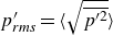 $p^\prime _{\textit{rms}} = {\langle \sqrt { \overline {p^{\prime 2}} } \rangle }$
of selected cases. The black circle symbol represents the wall
$p^\prime _{\textit{rms}} = {\langle \sqrt { \overline {p^{\prime 2}} } \rangle }$
of selected cases. The black circle symbol represents the wall $p^\prime _{\textit{rms}}$
predicted by the semi-empirical formula of Farabee & Casarella (Reference Farabee and Casarella1991). Dashed lines: spatio-temporally averaged streamwise velocity profiles; triangles mark the locations corresponding to the bulk convection velocity
$p^\prime _{\textit{rms}}$
predicted by the semi-empirical formula of Farabee & Casarella (Reference Farabee and Casarella1991). Dashed lines: spatio-temporally averaged streamwise velocity profiles; triangles mark the locations corresponding to the bulk convection velocity $U_{bc}/U_b$
.
$U_{bc}/U_b$
.

Figure 6. Long description
Two line graphs compare experimental measurements of wall-pressure fluctuations in single-phase flows. Panel A: A line graph shows profiles of the mean pressure. The x-axis is labeled y/h and the y-axis is labeled <p>/τw. Different colored lines represent various cases, with crosses denoting case SP. Panel B: A line graph displays profiles of the root-mean-square (r.m.s.) pressure fluctuations for selected cases. The x-axis is labeled y/h and the y-axis is labeled p rms/τw. Solid lines represent different cases, while dashed lines show spatio-temporally averaged streamwise velocity profiles. The black circle symbol represents the wall predicted by the semi-empirical formula of Farabee & Casarella (1991). Triangles mark the locations corresponding to the bulk convection velocity.
4.1. Mean pressure and pressure fluctuation intensity
The pressure fluctuation is defined as the instantaneous pressure minus the mean pressure. We therefore first examine the distribution of the mean pressure, $\langle p\rangle$
. Taking the spatio-temporal average of (2.3), neglecting the repulsive force and considering the wall-normal component, the averaged momentum equation can be simplified as
$\langle p\rangle$
. Taking the spatio-temporal average of (2.3), neglecting the repulsive force and considering the wall-normal component, the averaged momentum equation can be simplified as
 \begin{equation} 0 = - \frac {{\mathrm{d}\langle p\rangle }}{{\mathrm{d}y}} - \frac {{\mathrm{d}\langle \rho _m v'v'\rangle }}{{\mathrm{d}y}} + \frac {{\mathrm{d}\langle \tau ^{\textit{eff}}_{yy}\rangle }}{{\mathrm{d}y}} + \langle F^{\sigma }_{y}\rangle . \end{equation}
Here, the mean viscous contribution in $\langle \tau _{yy}\rangle$
is of the order of
$\langle \tau _{yy}\rangle$
is of the order of $10^{-3}\rho _l u_\tau ^2$
, while the SGS stress
$10^{-3}\rho _l u_\tau ^2$
, while the SGS stress $\langle \tau ^{\textit{SGS}}_{yy}\rangle$
is of the order of
$\langle \tau ^{\textit{SGS}}_{yy}\rangle$
is of the order of $10^{-4}\rho _l u_\tau ^2$
, as shown in Appendix B. The contribution associated with the effective wall-normal normal stress is several orders of magnitude smaller than
$10^{-4}\rho _l u_\tau ^2$
, as shown in Appendix B. The contribution associated with the effective wall-normal normal stress is several orders of magnitude smaller than $\langle \rho _m v'v'\rangle /(\rho _l u_\tau ^2)$
, thus, is negligible in both the single-phase and bubbly flows.
$\langle \rho _m v'v'\rangle /(\rho _l u_\tau ^2)$
, thus, is negligible in both the single-phase and bubbly flows.
For the single-phase flow, the surface-tension term is absent. The wall-normal gradient of mean pressure is then balanced by the gradient of the turbulent momentum. Integrating (4.1) gives
 \begin{equation} \langle p\rangle = \textrm {const.} - \rho _l \langle v'v'\rangle . \end{equation}
Thus, the mean pressure profile follows the distribution of $-\langle v'v'\rangle$
, as shown in figure 6(a), where
$-\langle v'v'\rangle$
, as shown in figure 6(a), where $\langle p\rangle$
has been shifted by a constant such that
$\langle p\rangle$
has been shifted by a constant such that $\langle p\rangle =0$
at the wall.
$\langle p\rangle =0$
at the wall.
For the bubbly flows, $\langle \rho _m v'v'\rangle$
remains close to its single-phase counterpart, as shown in figure 5. Therefore, near the wall, where the gas volume fraction is small and the mean surface-tension force
$\langle \rho _m v'v'\rangle$
remains close to its single-phase counterpart, as shown in figure 5. Therefore, near the wall, where the gas volume fraction is small and the mean surface-tension force $\langle F^{\sigma }_{y}\rangle$
is weak, the shape of
$\langle F^{\sigma }_{y}\rangle$
is weak, the shape of $\langle p\rangle$
is similar to that in the single-phase flow and exhibits a local minimum. In regions with a larger gas volume fraction, however,
$\langle p\rangle$
is similar to that in the single-phase flow and exhibits a local minimum. In regions with a larger gas volume fraction, however, $\langle F^{\sigma }_{y}\rangle$
becomes important, leading to a mean pressure profile that resembles the distribution of
$\langle F^{\sigma }_{y}\rangle$
becomes important, leading to a mean pressure profile that resembles the distribution of $\langle \alpha _g\rangle$
. Physically, this behaviour reflects the pressure jump across the gas–liquid interface induced by surface tension: in regions where bubbles are more frequently present, the averaged pressure is correspondingly increased.
$\langle \alpha _g\rangle$
. Physically, this behaviour reflects the pressure jump across the gas–liquid interface induced by surface tension: in regions where bubbles are more frequently present, the averaged pressure is correspondingly increased.
The profiles of the root-mean-square (r.m.s.) pressure fluctuations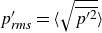 $p^\prime _{\textit{rms}} = {\langle \sqrt { \overline {p^{\prime 2}}}\rangle }$
, shown in figure 6(b) in solid lines, demonstrate that the pressure fluctuations in the bubbly flows are substantially larger than that in the single-phase flow except in the very near-wall region. At the wall,
$p^\prime _{\textit{rms}} = {\langle \sqrt { \overline {p^{\prime 2}}}\rangle }$
, shown in figure 6(b) in solid lines, demonstrate that the pressure fluctuations in the bubbly flows are substantially larger than that in the single-phase flow except in the very near-wall region. At the wall, $p^\prime _{\textit{rms}}(0)/\tau _w$
equals 2.25 (SP), 2.09 (B64D2), 2.08 (B128D2), 2.06 (B64D3) and 2.19 (B128D3), which are similar across all cases and are in reasonable agreement with the semi-empirical prediction of wall-pressure fluctuations 2.73 for single-phase flow (Farabee & Casarella Reference Farabee and Casarella1991), which is based on experimental and numerical data. A detailed analysis of the wall-pressure fluctuations is presented in § 5 based on wavenumber–frequency spectra and the associated convection velocity. In particular, the discussion of the 1-D spectra in § 5.4 will explain why
$p^\prime _{\textit{rms}}(0)/\tau _w$
equals 2.25 (SP), 2.09 (B64D2), 2.08 (B128D2), 2.06 (B64D3) and 2.19 (B128D3), which are similar across all cases and are in reasonable agreement with the semi-empirical prediction of wall-pressure fluctuations 2.73 for single-phase flow (Farabee & Casarella Reference Farabee and Casarella1991), which is based on experimental and numerical data. A detailed analysis of the wall-pressure fluctuations is presented in § 5 based on wavenumber–frequency spectra and the associated convection velocity. In particular, the discussion of the 1-D spectra in § 5.4 will explain why $p^\prime _{\textit{rms}}$
at the wall exhibits much smaller differences between single-phase and bubbly flows than those observed at other locations.
$p^\prime _{\textit{rms}}$
at the wall exhibits much smaller differences between single-phase and bubbly flows than those observed at other locations.
4.2. Decomposition of the instantaneous pressure fluctuation field
Referring to the Poisson equation of pressure fluctuations for variable-density flows derived by Chassaing et al. (Reference Chassaing, Antonia, Anselmet, Joly and Sarkar2002), the pressure fluctuation in the present multiphase incompressible flows is decomposed into the components
 \begin{equation} p' = p'_r + p'_s + p'_c + p'_v + p'_\sigma , \end{equation}
including the rapid pressure fluctuation $p'_r$
, slow pressure fluctuation
$p'_r$
, slow pressure fluctuation $p'_s$
, variable-density-related pressure fluctuation
$p'_s$
, variable-density-related pressure fluctuation $p'_c$
, viscosity-related pressure fluctuation
$p'_c$
, viscosity-related pressure fluctuation $p'_v$
and the surface-tension-related pressure fluctuation
$p'_v$
and the surface-tension-related pressure fluctuation $p'_\sigma$
. Each component satisfies the Poisson equation associated with the corresponding source term:
$p'_\sigma$
. Each component satisfies the Poisson equation associated with the corresponding source term:
 \begin{align} \boldsymbol{\nabla} ^2 p'_r = S_r = -2\frac {\partial ^2 \left (\overline {\rho _m}\,\bar {u}_{\!j}u'_i \right )} {\partial x_i \partial x_{\!j}}, \end{align}
 \begin{align} \boldsymbol{\nabla} ^2 p'_s = S_s = -\frac {\partial ^2 \left (\overline {\rho _m}u'_i u'_{\!j} - \overline {\rho _m}\,\overline {u'_i u'_{\!j}}\right )} {\partial x_i \partial x_{\!j}}, \end{align}
 \begin{equation} \boldsymbol{\nabla} ^2 p'_c = S_c = \frac {\partial ^2 \rho '_m}{\partial t^2} -2\frac {\partial ^2 \left [\left (\rho '_m u'_i - \overline {\rho '_m u'_i}\right )\bar {u}_{\!j}\right ]} {\partial x_i \partial x_{\!j}} -\frac {\partial ^2 \left (\rho '_m u'_i u'_{\!j} - \overline {\rho '_m u'_i u'_{\!j}}\right )} {\partial x_i \partial x_{\!j}} -\frac {\partial ^2 \left (\rho '_m \bar {u}_i \bar {u}_{\!j}\right )} {\partial x_i \partial x_{\!j}}, \end{equation}
 \begin{align} \boldsymbol{\nabla} ^2 p'_v = S_v = \frac {\partial ^2 \left (\tau ^{\textit{eff}}_{ij}-\overline {\tau ^{\textit{eff}}_{ij}}\right )} {\partial x_i \partial x_{\!j}}, \end{align}
 \begin{align} \boldsymbol{\nabla} ^2 p'_\sigma = S_\sigma = \frac {\partial }{\partial x_i} \left (\sigma \kappa \frac {\partial \alpha }{\partial x_i}\right ) - \overline { \frac {\partial }{\partial x_i} \left (\sigma \kappa \frac {\partial \alpha }{\partial x_i}\right ) }. \end{align}
The right-hand-side source term in the above Poisson equations are extracted from the numerical data. At the walls, the viscous component satisfies the boundary condition $\partial p'_v / \partial y = \partial \tau _{yi} / \partial x_i$
, whereas homogeneous Neumann boundary conditions are imposed for the remaining Poisson equations.
$\partial p'_v / \partial y = \partial \tau _{yi} / \partial x_i$
, whereas homogeneous Neumann boundary conditions are imposed for the remaining Poisson equations.
The first two equations, (4.4) and (4.5), take the same form as the classical Poisson equation of pressure fluctuations for single-phase incompressible flows (Kim Reference Kim1989), solving for the rapid pressure $p'_r$
with the linear source term
$p'_r$
with the linear source term $S_r$
and the slow pressure
$S_r$
and the slow pressure $p'_s$
with the nonlinear source term
$p'_s$
with the nonlinear source term $S_s$
, respectively. The difference from the single-phase case lies in the use of mean density
$S_s$
, respectively. The difference from the single-phase case lies in the use of mean density $\overline {\rho _m}$
in the present formulation. The solutions to these two Poisson equations are first performed for the single-phase case. The instantaneous contours of the pressure fluctuations associated with these two components are shown in figures 7(c) and 7(d). The slow component exhibits a stronger intensity than the rapid one, consistent with the well-established dominance of the slow pressure contribution in turbulent channel flows. To further verify the correctness of the solution, the superposition of these two components produces the pressure fluctuation shown in figure 7(b). The reconstructed field agrees almost perfectly with the pressure fluctuation obtained directly from the simulation (figure 7
a). This agreement confirms the reliability of the evaluation of the two incompressible source terms.
$\overline {\rho _m}$
in the present formulation. The solutions to these two Poisson equations are first performed for the single-phase case. The instantaneous contours of the pressure fluctuations associated with these two components are shown in figures 7(c) and 7(d). The slow component exhibits a stronger intensity than the rapid one, consistent with the well-established dominance of the slow pressure contribution in turbulent channel flows. To further verify the correctness of the solution, the superposition of these two components produces the pressure fluctuation shown in figure 7(b). The reconstructed field agrees almost perfectly with the pressure fluctuation obtained directly from the simulation (figure 7
a). This agreement confirms the reliability of the evaluation of the two incompressible source terms.
Instantaneous pressure fluctuation fields for the single-phase case: (a) instantaneous pressure fluctuations $p^\prime$
; (b) reconstructed field
$p^\prime$
; (b) reconstructed field $p^\prime _r + p^\prime _s$
; (c) the rapid component
$p^\prime _r + p^\prime _s$
; (c) the rapid component $p^\prime _r$
; (d) the slow component
$p^\prime _r$
; (d) the slow component $p^\prime _s$
. The wall-parallel plane is located at
$p^\prime _s$
. The wall-parallel plane is located at $y/h = 0.1$
and the z-normal plane is located at
$y/h = 0.1$
and the z-normal plane is located at $z/h = 0.1$
.
$z/h = 0.1$
.

The viscous source term $S_v$
in (4.7) is computed using the same viscous stress tensor appearing in the momentum equation, thereby ensuring numerical consistency.
$S_v$
in (4.7) is computed using the same viscous stress tensor appearing in the momentum equation, thereby ensuring numerical consistency.
The surface-tension-related source $S_\sigma$
in (4.8) is derived from the formulation of the momentum equation (2.3). In the present work, the term
$S_\sigma$
in (4.8) is derived from the formulation of the momentum equation (2.3). In the present work, the term $\boldsymbol{\nabla }\boldsymbol{\cdot }(\sigma \kappa \boldsymbol{\nabla }\alpha )$
is evaluated using a face-based finite-volume discretisation. The product of curvature
$\boldsymbol{\nabla }\boldsymbol{\cdot }(\sigma \kappa \boldsymbol{\nabla }\alpha )$
is evaluated using a face-based finite-volume discretisation. The product of curvature $\kappa$
and surface-tension coefficient
$\kappa$
and surface-tension coefficient $\sigma$
is interpolated to the cell faces, and the face-normal gradient
$\sigma$
is interpolated to the cell faces, and the face-normal gradient $\boldsymbol{\nabla} ^\perp _f \alpha$
is computed using the standard face-normal gradient operator. These quantities are assembled into a surface flux
$\boldsymbol{\nabla} ^\perp _f \alpha$
is computed using the standard face-normal gradient operator. These quantities are assembled into a surface flux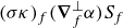 $(\sigma \kappa )_f (\boldsymbol{\nabla} ^\perp _f \alpha ) S_f$
, where the subscript
$(\sigma \kappa )_f (\boldsymbol{\nabla} ^\perp _f \alpha ) S_f$
, where the subscript $f$
denotes the face of the finite-volume cell and
$f$
denotes the face of the finite-volume cell and $S_f$
is the face area magnitude. The divergence is then obtained through a Gauss integration over the cell faces and normalised by the cell volume. This discretisation is identical to the finite-volume operators employed in the discrete solution of the governing equations (2.1)–(2.3), ensuring full consistency with the underlying numerical formulation.
$S_f$
is the face area magnitude. The divergence is then obtained through a Gauss integration over the cell faces and normalised by the cell volume. This discretisation is identical to the finite-volume operators employed in the discrete solution of the governing equations (2.1)–(2.3), ensuring full consistency with the underlying numerical formulation.
The terms involving the density fluctuations are grouped into the variable-density source $S_c$
. The form is consistent with the compressible terms in Chassaing et al. (Reference Chassaing, Antonia, Anselmet, Joly and Sarkar2002), while here the effects arise from density variations associated with the motion of bubbles. Because the mixture density exhibits sharp variation across the gas–liquid interface, evaluating the individual density-fluctuation-related terms is extremely sensitive to discretisation used in post-processing due to the presence of a second derivative, and may lead to significant numerical errors. Therefore, the combined contribution from density variation
$S_c$
. The form is consistent with the compressible terms in Chassaing et al. (Reference Chassaing, Antonia, Anselmet, Joly and Sarkar2002), while here the effects arise from density variations associated with the motion of bubbles. Because the mixture density exhibits sharp variation across the gas–liquid interface, evaluating the individual density-fluctuation-related terms is extremely sensitive to discretisation used in post-processing due to the presence of a second derivative, and may lead to significant numerical errors. Therefore, the combined contribution from density variation $S_c$
is estimated through the residual of the Poisson equation as
$S_c$
is estimated through the residual of the Poisson equation as $S_c = \boldsymbol{\nabla} ^2 p' - S_r - S_s - S_v - S_\sigma$
.
$S_c = \boldsymbol{\nabla} ^2 p' - S_r - S_s - S_v - S_\sigma$
.
Instantaneous pressure fluctuation fields for case B128D3: (a) instantaneous pressure fluctuations $p^\prime$
; (b) reconstructed field
$p^\prime$
; (b) reconstructed field $p^\prime _r + p^\prime _s + p^\prime _c + p^\prime _v + p^\prime _\sigma$
; (c) rapid-linear component
$p^\prime _r + p^\prime _s + p^\prime _c + p^\prime _v + p^\prime _\sigma$
; (c) rapid-linear component $p^\prime _r$
; (d) slow-nonlinear component
$p^\prime _r$
; (d) slow-nonlinear component $p^\prime _s$
; (e) variable-density-related component
$p^\prime _s$
; (e) variable-density-related component $p^\prime _c$
; (f) viscosity-related component
$p^\prime _c$
; (f) viscosity-related component $p^\prime _v$
; (g) surface-tension-related component
$p^\prime _v$
; (g) surface-tension-related component $p^\prime _\sigma$
. The wall-parallel plane is located at
$p^\prime _\sigma$
. The wall-parallel plane is located at $y/h=0.5$
, and the
$y/h=0.5$
, and the $z$
-normal plane is located at
$z$
-normal plane is located at $z/h=0.1$
.
$z/h=0.1$
.

Figure 8. Long description
Panel A: A heat map representing instantaneous pressure fluctuation. The color scale ranges from -20 to 20, with darker colors indicating lower values and lighter colors indicating higher values. The heat map shows a distribution of pressure fluctuations with some regions of high intensity. Panel B: A heat map showing the reconstructed field of pressure fluctuations. The color scale ranges from -20 to 20, similar to Panel A, with a similar distribution of high and low intensity regions. Panel C: A heat map depicting the rapid-linear component of pressure fluctuations. The color scale ranges from -10 to 10, with a more uniform distribution and fewer high-intensity regions compared to Panels A and B. Panel D: A heat map illustrating the slow-nonlinear component of pressure fluctuations. The color scale ranges from -10 to 10, showing a more dispersed pattern of fluctuations. Panel E: A heat map showing the variable-density-related component of pressure fluctuations. The color scale ranges from -20 to 20, with distinct regions of high and low intensity. Panel F: A heat map depicting the viscosity-related component of pressure fluctuations. The color scale ranges from -1 to 1, indicating a more subtle variation in pressure fluctuations. Panel G: A heat map illustrating the surface-tension-related component of pressure fluctuations. The color scale ranges from -20 to 20, with prominent regions of high intensity.
Figure 8 present the instantaneous pressure fluctuation decomposition for case B128D3 as an example. The reconstructed pressure fluctuation obtained from the Poisson equations, $p'_r + p'_s + p'_c + p'_v + p'_\sigma$
(figure 8
b), is compared with the pressure fluctuation directly obtained from the numerical simulation (figure 8
a). The two fields exhibit excellent agreement, both in their spatial structures and in quantitative pointwise comparisons, thereby demonstrating the accuracy of the Poisson solutions in (4.4)–(4.8) and the resulting pressure fluctuation components. In general, the pressure fluctuations are primarily associated with the presence of bubbles, with the largest magnitudes occurring in the region surrounding the bubbles.
$p'_r + p'_s + p'_c + p'_v + p'_\sigma$
(figure 8
b), is compared with the pressure fluctuation directly obtained from the numerical simulation (figure 8
a). The two fields exhibit excellent agreement, both in their spatial structures and in quantitative pointwise comparisons, thereby demonstrating the accuracy of the Poisson solutions in (4.4)–(4.8) and the resulting pressure fluctuation components. In general, the pressure fluctuations are primarily associated with the presence of bubbles, with the largest magnitudes occurring in the region surrounding the bubbles.
The rapid component $p'_r$
originates from the interaction between velocity fluctuations and the mean shear. Strong velocity fluctuations occur across the bubble interfaces due to the discontinuous flow characteristics inside and outside the bubbles. As a result, the rapid component is significantly stronger around the bubbles than in the pure liquid phase. In comparison, the slow component
$p'_r$
originates from the interaction between velocity fluctuations and the mean shear. Strong velocity fluctuations occur across the bubble interfaces due to the discontinuous flow characteristics inside and outside the bubbles. As a result, the rapid component is significantly stronger around the bubbles than in the pure liquid phase. In comparison, the slow component $p'_s$
provides the dominant contribution to the pressure fluctuations within the liquid regions, although the largest magnitudes still occur near the bubbles.
$p'_s$
provides the dominant contribution to the pressure fluctuations within the liquid regions, although the largest magnitudes still occur near the bubbles.
The variable-density component $p'_c$
is closely associated with density fluctuations induced by bubble motion. A characteristic pattern is observed in figure 8(e) around the bubbles: the pressure fluctuation is negative on the upstream side of the bubble and positive on the downstream side, consistent with the direction of bubble motion. Even in regions without bubbles,
$p'_c$
is closely associated with density fluctuations induced by bubble motion. A characteristic pattern is observed in figure 8(e) around the bubbles: the pressure fluctuation is negative on the upstream side of the bubble and positive on the downstream side, consistent with the direction of bubble motion. Even in regions without bubbles, $\rho '_m$
remains non-zero because the mean density is less than the liquid density.
$\rho '_m$
remains non-zero because the mean density is less than the liquid density.
The viscous contribution $p'_v$
, as shown in figure 8(f), remains small throughout the channel, with an amplitude more than one order of magnitude smaller than those of the other components. This behaviour is expected because it is associated with the Stokes pressure, which vanishes in incompressible flows and remains negligible in compressible flows (Gerolymos, Sénéchal & Vallet Reference Gerolymos, Sénéchal and Vallet2013).
$p'_v$
, as shown in figure 8(f), remains small throughout the channel, with an amplitude more than one order of magnitude smaller than those of the other components. This behaviour is expected because it is associated with the Stokes pressure, which vanishes in incompressible flows and remains negligible in compressible flows (Gerolymos, Sénéchal & Vallet Reference Gerolymos, Sénéchal and Vallet2013).
The surface-tension-related component $p'_\sigma$
clearly reveals the pressure difference between the interior and exterior of the bubbles, shown in figure 8(g), which is physically consistent with the Laplace pressure jump across the gas–liquid interface. This surface-tension contribution accounts for the dominant part of the pressure fluctuations in the bubbly flow; a similar prominence has been found in the momentum-equation budgets (du Cluzeau et al. Reference du Cluzeau, Bois and Toutant2019). As a result, the r.m.s. pressure fluctuations
$p'_\sigma$
clearly reveals the pressure difference between the interior and exterior of the bubbles, shown in figure 8(g), which is physically consistent with the Laplace pressure jump across the gas–liquid interface. This surface-tension contribution accounts for the dominant part of the pressure fluctuations in the bubbly flow; a similar prominence has been found in the momentum-equation budgets (du Cluzeau et al. Reference du Cluzeau, Bois and Toutant2019). As a result, the r.m.s. pressure fluctuations $p'_{\textit{rms}}$
in the bubbly flows becomes significantly larger over most of the channel compared with the single-phase case (figure 6). Both a higher gas volume fraction and a larger surface-tension force increase the capillary pressure jump across the bubble interface, which elevates the level of
$p'_{\textit{rms}}$
in the bubbly flows becomes significantly larger over most of the channel compared with the single-phase case (figure 6). Both a higher gas volume fraction and a larger surface-tension force increase the capillary pressure jump across the bubble interface, which elevates the level of $p'_{\textit{rms}}$
.
$p'_{\textit{rms}}$
.
4.3. Comparison of the source magnitudes of pressure fluctuations
The instantaneous pressure fluctuation decomposition discussed above reveals the spatial organisation of the different pressure fluctuation components. To further connect these pressure fields with their corresponding Poisson sources and to assess the relative importance of the different source mechanisms, we next examine the source terms in the pressure fluctuation Poisson equation.
We first consider their instantaneous spatial distributions. Figure 9 shows the instantaneous source terms for case B128D3 at the same time instant as that used in figure 8. The colour ranges are clipped to improve the visibility of the spatial structures. The total source term, $\boldsymbol{\nabla} ^2 p'$
, is mainly concentrated in the vicinity of the gas–liquid interfaces. Additional localised structures can also be observed in the small bubble wake regions and near the wall. The strong interfacial distribution results from the combined contributions of the different source terms, whereas the localised wake structures mainly arise from
$\boldsymbol{\nabla} ^2 p'$
, is mainly concentrated in the vicinity of the gas–liquid interfaces. Additional localised structures can also be observed in the small bubble wake regions and near the wall. The strong interfacial distribution results from the combined contributions of the different source terms, whereas the localised wake structures mainly arise from $S_r$
and
$S_r$
and $S_c$
. The near-wall distribution of
$S_c$
. The near-wall distribution of $\boldsymbol{\nabla} ^2 p'$
is mainly originated from the slow source term
$\boldsymbol{\nabla} ^2 p'$
is mainly originated from the slow source term $S_s$
. The viscous source term
$S_s$
. The viscous source term $S_v$
has a much smaller magnitude, consistent with the weak contribution of
$S_v$
has a much smaller magnitude, consistent with the weak contribution of $p'_v$
shown above. In particular,
$p'_v$
shown above. In particular, $S_\sigma$
is sharply localised at the gas–liquid interfaces and forms ring-like structures exactly along the bubble interfaces. These interfacial source structures, when inverted through the Poisson equation, give rise to the spatial distribution of
$S_\sigma$
is sharply localised at the gas–liquid interfaces and forms ring-like structures exactly along the bubble interfaces. These interfacial source structures, when inverted through the Poisson equation, give rise to the spatial distribution of $p'_\sigma$
, which represents the surface-tension-induced pressure jump across the bubble interface.
$p'_\sigma$
, which represents the surface-tension-induced pressure jump across the bubble interface.
Instantaneous source terms for case B128D3 at the same time instant as the snapshot shown in figure 8. (a) Laplacian of the pressure fluctuation, $\boldsymbol{\nabla} ^2 p^\prime$
; (b) rapid source term,
$\boldsymbol{\nabla} ^2 p^\prime$
; (b) rapid source term, $S_r$
; (c) slow source term,
$S_r$
; (c) slow source term, $S_s$
; (d) variable-density source term,
$S_s$
; (d) variable-density source term, $S_c$
; (e) viscous source term,
$S_c$
; (e) viscous source term, $S_v$
; and (f) surface-tension-related source term,
$S_v$
; and (f) surface-tension-related source term, $S_\sigma$
. The wall-parallel plane is located at
$S_\sigma$
. The wall-parallel plane is located at $y/h=0.5$
, and the
$y/h=0.5$
, and the $z$
-normal plane is located at
$z$
-normal plane is located at $z/h=0.1$
.
$z/h=0.1$
.

Profiles of the mean square of the source terms in the Poisson equations (4.4)–(4.8) for case B128D2 (solid lines) and B128D3 (dashed lines).

Figure 10. Long description
Panel: A line graph showing the profiles of the mean square of the source terms in the Poisson equations for cases B 128 D 2 and B 128 D 3. The horizontal axis represents y plus, ranging from 10 to the power of 0 to 10 to the power of 2. The vertical axis represents the mean-square of source terms divided by tau w squared delta n v to the power of 4, ranging from 10 to the power of -8 to 10 to the power of 0. The graph includes multiple lines representing different source terms: B 128 D 2 ((S r plus S s) squared) in red solid line, B 128 D 2 (S c squared) in blue solid line, B 128 D 2 (S v squared) in orange solid line, B 128 D 3 ((S r plus S s) squared) in red dashed line, and B 128 D 2 (S sigma squared) in yellow dashed line. The graph is divided into three regions: Viscous sublayer, Buffer layer, and Log layer. Each line shows different trends across these regions.

We then examine the intensity of the corresponding source terms in a statistical sense, taking cases B128D2 and B128D3 as examples. The spatio-temporally averaged mean-square values of the source terms as a function of the wall-normal coordinate $y^+$
are shown in figure 10. The following discussion is organised according to the classical division of the near-wall region into the viscous sublayer, buffer layer and logarithmic layer.
$y^+$
are shown in figure 10. The following discussion is organised according to the classical division of the near-wall region into the viscous sublayer, buffer layer and logarithmic layer.
Because only three grid points fall within the viscous sublayer, the detailed variation of the source terms in this region cannot be fully resolved, and the corresponding trends should therefore be interpreted with caution. Nevertheless, the available results suggest that the viscous contribution is comparable to the other terms very close to the wall. Moving away from the viscous sublayer, however, its magnitude rapidly decreases and becomes several orders of magnitude smaller than the other contributions. This behaviour is consistent with the fact that viscous effects are confined to the smallest scales and are primarily important in the immediate vicinity of the wall. The surface-tension source $S_\sigma$
becomes the dominant contribution among all source terms. The surface-tension term is determined by the bubble distribution and the interface curvature, which vary with bubble diameter and deformation across the channel. Bubbles in the near-wall region exhibit evident deformation, as shown in figure 2(c), resulting in large values of
$S_\sigma$
becomes the dominant contribution among all source terms. The surface-tension term is determined by the bubble distribution and the interface curvature, which vary with bubble diameter and deformation across the channel. Bubbles in the near-wall region exhibit evident deformation, as shown in figure 2(c), resulting in large values of $S_\sigma$
. Although the mean gas volume fraction
$S_\sigma$
. Although the mean gas volume fraction $\langle \alpha _g \rangle$
is low in this region, instantaneous flow-field visualisations in figure 1 reveal sporadic bubble passages, which may generate high local values in
$\langle \alpha _g \rangle$
is low in this region, instantaneous flow-field visualisations in figure 1 reveal sporadic bubble passages, which may generate high local values in $S_\sigma$
. Consequently, the layer averaged
$S_\sigma$
. Consequently, the layer averaged $\langle S^2_\sigma \rangle$
in this near-wall region exceeds that of other source terms because of these intermittent yet intense contributions.
$\langle S^2_\sigma \rangle$
in this near-wall region exceeds that of other source terms because of these intermittent yet intense contributions.
In the buffer layer, all source terms increase in magnitude compared with the near-wall region. A clear difference between cases B128D3 and B128D2 can already be observed, with larger values in B128D3. This trend is broadly consistent with the higher gas volume fraction and indicates a stronger bubble-induced modulation of the pressure fluctuation field.
In the logarithmic layer, the incompressible contribution (including both the rapid and slow components), the variable-density terms and the surface-tension-related terms are of comparable magnitude and together dominate the pressure fluctuations. This balance highlights that, in bubble-rich regions, the pressure fluctuation is governed by a combination of mechanisms, including shear-induced turbulent interactions, density variations associated with bubble motion and interfacial surface-tension effects. In contrast, the viscous term remains negligible throughout this region.
Overall, these results demonstrate that, unlike in single-phase flows where pressure fluctuations are governed by the incompressible rapid and slow terms, bubbly flows exhibit a multi-mechanism balance in which variable-density and surface-tension effects play equally important roles in the generation of pressure fluctuations.
Figure 11 shows the mean-square profiles of the incompressible source terms for cases B128D2, B128D3 and the single-phase flow (SP). In the bubbly flows, the incompressible sources are smaller than those in the single-phase case within the viscous sublayer, but they exhibit a markedly different trend farther away from the wall. In the single-phase case, the incompressible source terms attain their maximum within the buffer layer and subsequently decrease towards the channel centre. In contrast, for the bubbly cases, the source terms continue to increase beyond the buffer layer and reach their largest values in the logarithmic and core regions. In the channel core, the incompressible source terms become significantly larger than those in the single-phase flow. This behaviour is consistent with the instantaneous observations discussed in figures 7 and 8, where $p'_r$
and
$p'_r$
and $p'_s$
remain strong in the core region of the bubbly flow, while in single-phase flow they both decay in the channel core.
$p'_s$
remain strong in the core region of the bubbly flow, while in single-phase flow they both decay in the channel core.
A further distinction arises in the relative importance of the linear and nonlinear contributions. In bubbly cases, the linear term becomes larger in the logarithmic region ( $y^+\gt 55$
for case B128D3 and
$y^+\gt 55$
for case B128D3 and $y^+\gt 40$
for case B128D2), contrary to the common understanding that the nonlinear term dominates throughout the channel in single-phase flows (Kim Reference Kim1989; Chang III et al. Reference Chang, Piomelli and Blake1999). Referring to its expression, the larger linear term may arise from the gradient of the mean density in combination with the mean velocity. This finding emphasises that the bubble-induced contribution to pressure fluctuations originates primarily from variable-density effects, involving not only density fluctuations but also the spatial gradient of the mean density.
$y^+\gt 40$
for case B128D2), contrary to the common understanding that the nonlinear term dominates throughout the channel in single-phase flows (Kim Reference Kim1989; Chang III et al. Reference Chang, Piomelli and Blake1999). Referring to its expression, the larger linear term may arise from the gradient of the mean density in combination with the mean velocity. This finding emphasises that the bubble-induced contribution to pressure fluctuations originates primarily from variable-density effects, involving not only density fluctuations but also the spatial gradient of the mean density.
These results indicate that the pressure fluctuations induced by bubbles originate primarily from two mechanisms: (i) a density-related effect, including the spatial variation of mean density and the interfacial jump of density, and (ii) a surface-tension-related effect, inducing a pressure difference across bubble interfaces. These combined effects constitute a fundamental distinction from single-phase flows, in which pressure fluctuations are predominantly governed by incompressible turbulence dynamics.
5. Wavenumber–frequency spectra of wall-pressure fluctuations
5.1. The method for calculating the wavenumber–frequency spectrum
The wall-pressure fluctuations are analysed in terms of the wavenumber–frequency spectrum, which is calculated using the method described by Choi & Moin (Reference Choi and Moin1990) and then by Yang & Yang (Reference Yang and Yang2022). In this subsection we briefly review the calculation method.
The sequence of the 3-D wall-pressure fluctuations, denoted by $p'(x, z, t)$
, is discretised into
$p'(x, z, t)$
, is discretised into $M$
segments in time, each with a 50 % overlap with its adjacent segment. Each segment contains a number of successive snapshots with
$M$
segments in time, each with a 50 % overlap with its adjacent segment. Each segment contains a number of successive snapshots with $N_t = 256$
for the single-phase case and
$N_t = 256$
for the single-phase case and $N_t = 500$
for bubbly cases. Subsequently, a Fourier transform is performed within each segment in both the streamwise and spanwise directions, as well as in time, to extract the Fourier components. Given that the data are discretised on a grid, the discrete Fourier transform is employed to calculate the Fourier modes
$N_t = 500$
for bubbly cases. Subsequently, a Fourier transform is performed within each segment in both the streamwise and spanwise directions, as well as in time, to extract the Fourier components. Given that the data are discretised on a grid, the discrete Fourier transform is employed to calculate the Fourier modes $\widehat {p^\prime }( {k_x},{k_z},\omega )$
as
$\widehat {p^\prime }( {k_x},{k_z},\omega )$
as
 \begin{eqnarray} \widehat {p^\prime }\left ( {{k_x},{k_z},\omega } \right ) & = & \frac {1}{{{N_x}{N_z}{N_t}{\sqrt {C_w}}}}\sum \limits _{l = 0}^{{N_x} - 1} {\sum \limits _{m = 0}^{{N_z} - 1} {\sum \limits _{n = 0}^{{N_t} - 1} w } } \left ( {\frac {{nT}}{{{N_t}}}} \right )p^\prime \left ( {\frac {{l{L_x}}}{{{N_x}}},{\mkern 1mu} \frac {{m{L_z}}}{{{N_z}}},{\mkern 1mu} \frac {{nT}}{{{N_t}}}} \right ) \nonumber \\ && \times \exp \left ( { - {\textrm {i}}\left ( {\frac {{l{L_x}}}{{{N_x}}}{k_x} + \frac {{m{L_z}}}{{{N_z}}}{k_z} + \frac {{nT}}{{{N_t}}}\omega } \right )} \right )\!, \end{eqnarray}
 \begin{equation} C_w=\frac {1}{{{N_t}}}\sum \limits _{n = 0}^{{N_t} - 1} \; {w^2}\left ( {{\mkern 1mu} \frac {{nT}}{{{N_t}}}} \right )\!, \end{equation}
where $k_x$
and
$k_x$
and $k_z$
are the streamwise and spanwise wavenumbers,
$k_z$
are the streamwise and spanwise wavenumbers, $\omega$
is the frequency,
$\omega$
is the frequency, $C_w$
is the window constant to keep the r.m.s. of
$C_w$
is the window constant to keep the r.m.s. of $p^\prime$
unchanged after applying the standard Hanning window function
$p^\prime$
unchanged after applying the standard Hanning window function $w(t)$
,
$w(t)$
, $T = {N_t} \times {T_s}$
is the time duration of each segment, with
$T = {N_t} \times {T_s}$
is the time duration of each segment, with $T_s$
being the sampling interval. The 3-D wavenumber–frequency spectrum of wall-pressure fluctuations is defined as
$T_s$
being the sampling interval. The 3-D wavenumber–frequency spectrum of wall-pressure fluctuations is defined as
 \begin{equation} {\varPhi _{p^\prime p^\prime }}({k_x},{k_z},\omega ) = \frac {{\overline {\widehat {p^\prime }({k_x},{k_z},\omega ){{\widehat {p^\prime }}^*}({k_x},{k_z},\omega )} }}{{\varDelta {k_x}\varDelta {k_z}\varDelta \omega }}, \end{equation}
where the superscript $*$
denotes the complex conjugate,
$*$
denotes the complex conjugate, $\varDelta k_x=2\pi /L_x$
and
$\varDelta k_x=2\pi /L_x$
and $\varDelta k_z=2\pi /L_z$
are the resolution of the streamwise wavenumber and spanwise wavenumber, respectively, and
$\varDelta k_z=2\pi /L_z$
are the resolution of the streamwise wavenumber and spanwise wavenumber, respectively, and $\varDelta \omega =2\pi /T$
is the frequency resolution. Here, the overbar symbol represents the mean value over the entire set of
$\varDelta \omega =2\pi /T$
is the frequency resolution. Here, the overbar symbol represents the mean value over the entire set of $M$
segments. The reduced-dimension spectra are calculated by integrating the 3-D wavenumber–frequency spectrum, for example, applying
$M$
segments. The reduced-dimension spectra are calculated by integrating the 3-D wavenumber–frequency spectrum, for example, applying
 \begin{equation} {\varPhi _{p^\prime p^\prime }}({k_x},\omega ) = \int {{\varPhi _{p^\prime p^\prime }}({k_x},{k_z},\omega ){\mathrm{d}}{k_z}} \end{equation}
to obtain the 2-D spectrum and
 \begin{equation} {\varPhi _{p^\prime p^\prime }}\left ( {{k_x}} \right ) = \int _{ - \infty }^\infty {\int _{ - \infty }^\infty {{\varPhi _{p^\prime p^\prime }}} } \left ( {{k_x},{k_z},\omega } \right ){\mkern 1mu} {\mathrm{d}}{k_z}{\mkern 1mu} {\mathrm{d}}\omega \end{equation}
to obtain the 1-D spectrum. The validation of the wavenumber–frequency spectrum for single-phase flows is provided in Appendix A.
5.2. Two-dimensional spectra
An overview of the characteristics of wavenumber–frequency spectra for pressure fluctuations through three representative cases, B64D3, B128D3 and SP, is illustrated in figure 12. Among all spectra, particular attention is given to the streamwise wavenumber–frequency spectrum $\varPhi _{p^\prime p^\prime }(k_x, \omega )$
, as it captures the distribution characteristics of wall-pressure fluctuations across different frequency components along the flow direction. The ridge in the spectrum denotes the convection process of energy-containing wall-pressure fluctuations. Compared with the spectrum in case SP (figure 12
c), which exclusively exhibits a single ridge, it is evident that the spectra in bubbly cases retain the fundamental characteristics of turbulent flow in the liquid phase. Additionally, a new convective ridge emerges, as can be more clearly observed from the contour lines in the
$\varPhi _{p^\prime p^\prime }(k_x, \omega )$
, as it captures the distribution characteristics of wall-pressure fluctuations across different frequency components along the flow direction. The ridge in the spectrum denotes the convection process of energy-containing wall-pressure fluctuations. Compared with the spectrum in case SP (figure 12
c), which exclusively exhibits a single ridge, it is evident that the spectra in bubbly cases retain the fundamental characteristics of turbulent flow in the liquid phase. Additionally, a new convective ridge emerges, as can be more clearly observed from the contour lines in the $(k_x,\omega )$
plane shown in figures 12(a) and 12(b). This feature, hereafter referred to as the bubble convection ridge, will later be shown to be associated with bubble-induced dynamics, distinct from the turbulence convection ridge in single-phase flows. The solid black line along the convection ridge represents the most energetic pressure fluctuation convection with its expression
$(k_x,\omega )$
plane shown in figures 12(a) and 12(b). This feature, hereafter referred to as the bubble convection ridge, will later be shown to be associated with bubble-induced dynamics, distinct from the turbulence convection ridge in single-phase flows. The solid black line along the convection ridge represents the most energetic pressure fluctuation convection with its expression $\varPhi _{p^\prime p^\prime }(k_x^*, \omega ^*)$
, where
$\varPhi _{p^\prime p^\prime }(k_x^*, \omega ^*)$
, where $\omega ^* / k_x^* = U_{bc}$
with
$\omega ^* / k_x^* = U_{bc}$
with $U_{bc}$
denoting the bulk convection velocity. On the two vertical planes (
$U_{bc}$
denoting the bulk convection velocity. On the two vertical planes ( $k_x-$
and
$k_x-$
and $\omega -$
planes), variations of spectral magnitude with respect to frequency
$\omega -$
planes), variations of spectral magnitude with respect to frequency $\omega$
at a fixed streamwise wavenumber
$\omega$
at a fixed streamwise wavenumber $k_x^*$
and wavenumber
$k_x^*$
and wavenumber $k_x$
at a fixed frequency
$k_x$
at a fixed frequency $\omega ^*$
are illustrated. Projections of the convection ridge onto the two vertical coordinate planes indicate variations in the approximate maximum pressure fluctuation intensities as functions of wavenumber and frequency. For all cases, the maximum intensity decreases with increasing wavenumber and frequency.
$\omega ^*$
are illustrated. Projections of the convection ridge onto the two vertical coordinate planes indicate variations in the approximate maximum pressure fluctuation intensities as functions of wavenumber and frequency. For all cases, the maximum intensity decreases with increasing wavenumber and frequency.
Three-dimensional profiles of wavenumber–frequency spectrum $\varPhi _{p^\prime p^\prime }( k_x,\omega )$
and the contours for case (a) B64D3, (b) B128D3, and (c) SP. The solid black line is the ridge line with its horizontal coordinates
$\varPhi _{p^\prime p^\prime }( k_x,\omega )$
and the contours for case (a) B64D3, (b) B128D3, and (c) SP. The solid black line is the ridge line with its horizontal coordinates $U_{bc}=\omega /k_x$
. The projections of the ridge line onto the
$U_{bc}=\omega /k_x$
. The projections of the ridge line onto the $k_x$
plane (dot–dashed black line) and the
$k_x$
plane (dot–dashed black line) and the $\omega$
plane (dashed black line) are plotted. The spectrum for a fixed streamwise wavenumber
$\omega$
plane (dashed black line) are plotted. The spectrum for a fixed streamwise wavenumber $\varPhi _{p^\prime p^\prime }(k_x^*,\omega )$
is plotted as a dot–dashed line and for a fixed frequency,
$\varPhi _{p^\prime p^\prime }(k_x^*,\omega )$
is plotted as a dot–dashed line and for a fixed frequency, $\varPhi _{p^\prime p^\prime }(k_x,\omega ^*)$
is plotted as a dashed line.
$\varPhi _{p^\prime p^\prime }(k_x,\omega ^*)$
is plotted as a dashed line.

Figure 12. Long description
Panel C: A 3D plot depicting the wavenumber-frequency spectrum profiles and contours for case SP. The horizontal axis represents the streamwise wavenumber kxh, the vertical axis represents the frequency omega h divided by Ub, and the third axis represents the logarithm of the spectrum. The solid black line indicates the ridge line, with its projections onto the kxh plane shown as a dot-dashed black line and onto the omega h divided by Ub plane shown as a dashed black line. The spectrum for a fixed streamwise wavenumber is plotted as a dot-dashed line, and for a fixed frequency, it is plotted as a dashed line. The plot shows a peak around kxh of 100 and omega h divided by Ub of 0, with the spectrum values decreasing as you move away from this peak.
For clarity, figure 13(a–d) presents the contours of the 2-D wavenumber–frequency spectrum $\varPhi _{p^\prime p^\prime } ( k_x,\omega )$
for bubbly cases. The general features observed in cases B64D2 and B128D2 are similar to those of case SP (figure 22), primarily exhibiting the turbulence convection ridge. In cases B64D3 and B128D3, a distinct secondary convection ridge, that is, the bubble convection ridge, emerges alongside the primary turbulence-related ridge. This feature is attributed to bubble-induced pressure fluctuations based on the following evidence. First, as the gas volume fraction increases, the greater concentration of bubbles near the wall leads to a more pronounced ridge with higher spectral magnitudes and broader bandwidth, consistent with intuitive physical expectations. Second, the bubble convection ridge exhibits a markedly steeper slope and extends toward higher wavenumbers and frequencies, clearly distinguishing it from the turbulence convection ridge.
$\varPhi _{p^\prime p^\prime } ( k_x,\omega )$
for bubbly cases. The general features observed in cases B64D2 and B128D2 are similar to those of case SP (figure 22), primarily exhibiting the turbulence convection ridge. In cases B64D3 and B128D3, a distinct secondary convection ridge, that is, the bubble convection ridge, emerges alongside the primary turbulence-related ridge. This feature is attributed to bubble-induced pressure fluctuations based on the following evidence. First, as the gas volume fraction increases, the greater concentration of bubbles near the wall leads to a more pronounced ridge with higher spectral magnitudes and broader bandwidth, consistent with intuitive physical expectations. Second, the bubble convection ridge exhibits a markedly steeper slope and extends toward higher wavenumbers and frequencies, clearly distinguishing it from the turbulence convection ridge.
The 2-D spectrum in the streamwise wavenumber and frequency normalised as $\textrm {log}_{10}[\varPhi _{p^\prime p^\prime }(k_x,\omega )u_\tau /(\tau _w^2h^2)]$
for cases (a) B64D2, (b) B128D2, (c) B64D3, and (d) B128D3. The 2-D spectrum
$\textrm {log}_{10}[\varPhi _{p^\prime p^\prime }(k_x,\omega )u_\tau /(\tau _w^2h^2)]$
for cases (a) B64D2, (b) B128D2, (c) B64D3, and (d) B128D3. The 2-D spectrum $\varPhi _{p^\prime H}(k_x,\omega )$
of case (e) B64D3 and (f) B128D3.
$\varPhi _{p^\prime H}(k_x,\omega )$
of case (e) B64D3 and (f) B128D3.

The wavenumber–frequency spectrum of pressure fluctuations at fixed wavenumbers $\varPhi _{p^\prime p^\prime }(k_x^*,\omega )$
with
$\varPhi _{p^\prime p^\prime }(k_x^*,\omega )$
with $k_x^* h=27,35,50$
and 100.
$k_x^* h=27,35,50$
and 100.

Figure 14. Long description
Four line graphs depict the wavenumber-frequency spectrum of pressure fluctuations at fixed wavenumbers. Panel A: The line graph shows the spectrum for kxh equal to 27. The x-axis represents the non-dimensional frequency, ωh/U_b, ranging from -120 to 20. The y-axis represents the non-dimensional spectrum, Φp’p’(kx*, ω)uτ/(τw^2h^2), ranging from -12 to -4. Different colored lines represent different datasets: B64D2, B128D2, B64D3, B128D3, and SP. Panel B: The line graph shows the spectrum for kxh equal to 35. The axes and datasets are the same as in Panel A. Panel C: The line graph shows the spectrum for kxh equal to 50. The axes and datasets are the same as in Panel A. Panel D: The line graph shows the spectrum for kxh equal to 100. The axes and datasets are the same as in Panel A. Annotations indicate bubble-induced and turbulence-induced regions.
To further substantiate the bubble-induced nature of this secondary ridge, we employ a cross-correlation analysis to explicitly link the observed convective ridge in $\varPhi _{p^\prime p^\prime } ( k_x,\omega )$
for cases B64D3 and B128D3 to actual bubble motion. In order to calculate the cross-correlation function between the wall-pressure fluctuation and the distance of bubble from the wall, we define a function
$\varPhi _{p^\prime p^\prime } ( k_x,\omega )$
for cases B64D3 and B128D3 to actual bubble motion. In order to calculate the cross-correlation function between the wall-pressure fluctuation and the distance of bubble from the wall, we define a function $H(x,z,t)$
to measure the height of the bubble surface such that a larger value corresponds to a bubble closer to the wall, taking the
$H(x,z,t)$
to measure the height of the bubble surface such that a larger value corresponds to a bubble closer to the wall, taking the $y = 0$
wall as an example,
$y = 0$
wall as an example,
 \begin{equation} H(x,z,t)=2h-y_b(x,z,t), \end{equation}
where $y_b(x,z,t)$
denotes the
$y_b(x,z,t)$
denotes the $y$
coordinate of the lowest bubble interface. As bubbles move, the function
$y$
coordinate of the lowest bubble interface. As bubbles move, the function $H$
and
$H$
and $y_b$
vary with spatial coordinates
$y_b$
vary with spatial coordinates $(x, z)$
and time
$(x, z)$
and time $t$
. If no bubble exists at a specific
$t$
. If no bubble exists at a specific $(x, z)$
coordinate,
$(x, z)$
coordinate, $y_b$
is set to
$y_b$
is set to $2h$
, resulting in
$2h$
, resulting in $H=0$
.
$H=0$
.
The 2-D cross-correlation function between the wall-pressure fluctuation $p^\prime$
and the bubble height function
$p^\prime$
and the bubble height function $H$
in the streamwise distance
$H$
in the streamwise distance $\xi$
and time interval
$\xi$
and time interval $\tau$
is defined as
$\tau$
is defined as
 \begin{equation} {R_{p^\prime H}}\left ( {\xi ,\tau } \right ) = \frac {1}{{{N_z}}}\sum \limits _z {\left \langle {p^\prime \left ( {x,y=0,z,t} \right )H\left ( {x + \xi ,z,t + \tau } \right )} \right \rangle } , \end{equation}
where the angular brackets denote the ensemble average over all $x$
and
$x$
and $t$
. The normalised 2-D cross-correlation function
$t$
. The normalised 2-D cross-correlation function $R_{p^\prime H}(\xi ,\tau )/R_{p^\prime H}(0,0)$
is converted into the spectrum
$R_{p^\prime H}(\xi ,\tau )/R_{p^\prime H}(0,0)$
is converted into the spectrum $\varPhi _{p^\prime H} ( k_x,\omega )$
through a Fourier transform. Figures 13(e) and 13(f) present the pseudocolour plots of the spectrum
$\varPhi _{p^\prime H} ( k_x,\omega )$
through a Fourier transform. Figures 13(e) and 13(f) present the pseudocolour plots of the spectrum $\varPhi _{p^\prime H} (k_x,\omega )$
for cases B64D3 and B128D3. For case B64D3, the spectrum
$\varPhi _{p^\prime H} (k_x,\omega )$
for cases B64D3 and B128D3. For case B64D3, the spectrum $\varPhi _{p^\prime H} ( k_x,\omega )$
exhibits a narrow ridge whose shape and slope closely resemble those of the bubble convection ridge in
$\varPhi _{p^\prime H} ( k_x,\omega )$
exhibits a narrow ridge whose shape and slope closely resemble those of the bubble convection ridge in $\varPhi _{p^\prime p^\prime } ( k_x,\omega )$
in figure 13(c), while the broader turbulence convection ridge is excluded through the cross-correlation procedure. For case B128D3, the ridge in
$\varPhi _{p^\prime p^\prime } ( k_x,\omega )$
in figure 13(c), while the broader turbulence convection ridge is excluded through the cross-correlation procedure. For case B128D3, the ridge in $\varPhi _{p^\prime H} ( k_x,\omega )$
correspondingly becomes broader and exhibits higher intensity like the changes in
$\varPhi _{p^\prime H} ( k_x,\omega )$
correspondingly becomes broader and exhibits higher intensity like the changes in $\varPhi _{p^\prime p^\prime } ( k_x,\omega )$
in figure 13(d). This supports the association of the secondary ridge in
$\varPhi _{p^\prime p^\prime } ( k_x,\omega )$
in figure 13(d). This supports the association of the secondary ridge in $\varPhi _{p^\prime p^\prime } ( k_x,\omega )$
with bubble-induced pressure fluctuations.
$\varPhi _{p^\prime p^\prime } ( k_x,\omega )$
with bubble-induced pressure fluctuations.
The contour in figure 13 presents the morphology of the bubble convection ridge and turbulence convection ridge, while figure 14 provides quantitative cross-sectional views of $\varPhi _{p^\prime p^\prime }(k_x, \omega )$
at fixed streamwise wavenumbers
$\varPhi _{p^\prime p^\prime }(k_x, \omega )$
at fixed streamwise wavenumbers $k_x^*$
. Overall, the magnitude of the bubble convection ridge exceeds that of the turbulence ridge roughly at a certain wavenumber. The bubble convection ridge becomes more pronounced in the superconvective region (higher wavenumber or frequency region). In contrast, the ridge magnitudes in cases with a low gas volume fraction, i.e. B64D2 and B128D2, are lower than those in the SP case, with minor differences in the low wavenumber or frequency region but significant deviation in the superconvective region. The influence of bubbles is evident in two main aspects. First, a higher volume fraction leads to more bubbles towards the wall, resulting in stronger bubble-induced wall-pressure fluctuation, which is specifically reflected in the higher spectral magnitude and broader bandwidth observed in case B128D3 compared with case B64D3. Second, as shown in figures 14(a) and 14(c), the bubble ridge in B128D3 emerges at a lower wavenumber, surpassing the turbulence ridge at
$k_x^*$
. Overall, the magnitude of the bubble convection ridge exceeds that of the turbulence ridge roughly at a certain wavenumber. The bubble convection ridge becomes more pronounced in the superconvective region (higher wavenumber or frequency region). In contrast, the ridge magnitudes in cases with a low gas volume fraction, i.e. B64D2 and B128D2, are lower than those in the SP case, with minor differences in the low wavenumber or frequency region but significant deviation in the superconvective region. The influence of bubbles is evident in two main aspects. First, a higher volume fraction leads to more bubbles towards the wall, resulting in stronger bubble-induced wall-pressure fluctuation, which is specifically reflected in the higher spectral magnitude and broader bandwidth observed in case B128D3 compared with case B64D3. Second, as shown in figures 14(a) and 14(c), the bubble ridge in B128D3 emerges at a lower wavenumber, surpassing the turbulence ridge at $k_x h \approx 27$
, whereas in B64D3, it is
$k_x h \approx 27$
, whereas in B64D3, it is $k_x h \approx 50$
. These wavenumbers correspond to scales of
$k_x h \approx 50$
. These wavenumbers correspond to scales of $k_x D_b = \textit {O}(8{\sim} 15)$
, i.e. wavelengths of roughly 0.8
$k_x D_b = \textit {O}(8{\sim} 15)$
, i.e. wavelengths of roughly 0.8 $D_b$
–0.4
$D_b$
–0.4 $D_b$
. This indicates that bubble motion enhances pressure fluctuations at scales comparable to the bubble size, further supporting the interpretation that this spectral ridge originates from bubble-induced motions.
$D_b$
. This indicates that bubble motion enhances pressure fluctuations at scales comparable to the bubble size, further supporting the interpretation that this spectral ridge originates from bubble-induced motions.
For the low gas volume fraction case, B64D2, the magnitude of the wavenumber–frequency spectrum of pressure fluctuation is found to be suppressed. This behaviour can be partly explained by the distribution of turbulent coherent structures over the channel wall. The $Q$
-criterion is utilised to identify vortices, with results presented in figure 15 for the cases SP, B64D2 and B128D3. Under an identical
$Q$
-criterion is utilised to identify vortices, with results presented in figure 15 for the cases SP, B64D2 and B128D3. Under an identical $Q$
value, the present numerical results show that introducing bubbles to the channel disrupts and reduces considerably the coherence of the longitudinal vortex structures near the wall. In the core region of the channel, bubble-induced turbulence dominates over the shear-induced turbulence. Here, the vortices in both the wake region and near the bubble surface are smaller in size but denser and more intense than those in the single-phase case. In addition, as shown by the visualisation of vortices generated on the bubble surfaces, the vortex layers are relatively thin. The interfacial vorticity is confined in a boundary layer of thickness
$Q$
value, the present numerical results show that introducing bubbles to the channel disrupts and reduces considerably the coherence of the longitudinal vortex structures near the wall. In the core region of the channel, bubble-induced turbulence dominates over the shear-induced turbulence. Here, the vortices in both the wake region and near the bubble surface are smaller in size but denser and more intense than those in the single-phase case. In addition, as shown by the visualisation of vortices generated on the bubble surfaces, the vortex layers are relatively thin. The interfacial vorticity is confined in a boundary layer of thickness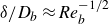 $\delta /D_b \approx \textit{Re}_b^{-1/2}$
(Riboux, Legendre & Risso Reference Riboux, Legendre and Risso2013). Accordingly, the present mesh resolution of
$\delta /D_b \approx \textit{Re}_b^{-1/2}$
(Riboux, Legendre & Risso Reference Riboux, Legendre and Risso2013). Accordingly, the present mesh resolution of $D_b /\varDelta \geqslant 30$
captures the interfacial vorticity with reasonable accuracy for
$D_b /\varDelta \geqslant 30$
captures the interfacial vorticity with reasonable accuracy for $\textit{Re}_b \sim 50$
, as discussed in Appendix D.
$\textit{Re}_b \sim 50$
, as discussed in Appendix D.
The anisotropic characteristics of flow structures can be qualitatively revealed according to the 2-D wavenumber spectrum $\varPhi _{p^\prime p^\prime }(k_x,k_z)$
, as shown in figure 16. For case SP, the isopleths are elongated in the spanwise direction, indicating that the flow structures contributing to wall-pressure fluctuations are more extended spanwise than streamwise – a feature also reported by Choi & Moin (Reference Choi and Moin1990). In the bubbly cases, the isopleth shapes in low gas volume fraction cases (B64D2 and B128D2) remain similar to those in the single-phase flow. In contrast, cases B64D3 and B128D3 exhibit noticeable changes in the isopleth patterns: the low-magnitude contours bulge toward the
$\varPhi _{p^\prime p^\prime }(k_x,k_z)$
, as shown in figure 16. For case SP, the isopleths are elongated in the spanwise direction, indicating that the flow structures contributing to wall-pressure fluctuations are more extended spanwise than streamwise – a feature also reported by Choi & Moin (Reference Choi and Moin1990). In the bubbly cases, the isopleth shapes in low gas volume fraction cases (B64D2 and B128D2) remain similar to those in the single-phase flow. In contrast, cases B64D3 and B128D3 exhibit noticeable changes in the isopleth patterns: the low-magnitude contours bulge toward the $k_x$
direction at low
$k_x$
direction at low $k_z$
wavenumbers, indicating that bubbles amplify the spectral components associated with large spanwise scales and small streamwise scales.
$k_z$
wavenumbers, indicating that bubbles amplify the spectral components associated with large spanwise scales and small streamwise scales.
Isosurfaces of the $Q$
-criterion (
$Q$
-criterion ( $Q = 7 \times 10^4$
), coloured in teal, are shown for (a) SP, (b) B64D2, (c) B128D3, with a zoomed-out view of two adjacent bubbles interacting with wall-generated vortical structures. The red plane indicates the plane at
$Q = 7 \times 10^4$
), coloured in teal, are shown for (a) SP, (b) B64D2, (c) B128D3, with a zoomed-out view of two adjacent bubbles interacting with wall-generated vortical structures. The red plane indicates the plane at $y^+=30$
. Translucent spheres represent the instantaneous bubble positions.
$y^+=30$
. Translucent spheres represent the instantaneous bubble positions.

The 2-D wavenumber spectrum ${\textrm {log}_{10}}[\varPhi _{p^\prime p^\prime }(k_x,k_z)/(\tau _w^2h^2)]$
for cases: (a) B64D2, (b) B128D2, (c) B64D3, (d) B128D3, and (e) SP.
${\textrm {log}_{10}}[\varPhi _{p^\prime p^\prime }(k_x,k_z)/(\tau _w^2h^2)]$
for cases: (a) B64D2, (b) B128D2, (c) B64D3, (d) B128D3, and (e) SP.

5.3. Convection velocity of the 2-D spectrum
Convection velocity is a key parameter that can be extracted from the convection ridge in the wavenumber–frequency spectrum. It represents the propagation speed of pressure fluctuations correlated with coherent motions. In practical applications, it can also provide a mapping between spatial and temporal quantities. According to the early experimental data (Willmarth & Wooldridge Reference Willmarth and Wooldridge1962), the convection velocity of the maximal energy-contained eddies ranges from 0.56 to 0.83 times the free-stream velocity. Since Taylor’s hypothesis is not applicable in the near-wall region, the convection velocity, which should depend on the scale of flow structures, is not constant. The distinct characteristics of the bubble-induced convection ridge, as compared with the turbulence-induced ridge, indicate that multiple types of coherent motions coexist. In this section we investigate the scale-dependent convection velocity of wall-pressure fluctuation.
The streamwise-wavenumber-dependent convection velocity can be calculated by
 \begin{equation} {U_c}\!\left ( {{k_x}} \right ) = -\frac {{\int {\omega \varPhi ({k_x},\omega ){\mkern 1mu} } {\mathrm{d}}\omega }}{{{k_x}\int {\varPhi ({k_x},\omega ){\mkern 1mu} } {\mathrm{d}}\omega }}, \end{equation}
which is equivalent to searching the position of the centre of gravity in the frequency spectrum at a given wavenumber $k_x^*$
(del Álamo & Jiménez Reference del Álamo and Jiménez2009). As shown in figure 17(a), the velocities in case SP decrease with increasing wavenumber, which agrees with previous studies (e.g. Choi & Moin (Reference Choi and Moin1990)) and align with the empirical curve in Panton & Linebarger (Reference Panton and Linebarger1974). This variation is attributed to the higher convection velocity of larger-scale flow structures originating in the outer layer, while smaller-scale structures near the wall exhibit a lower velocity. For case B64D2, the shape of the 2-D spectrum and the resulting convection velocity
$k_x^*$
(del Álamo & Jiménez Reference del Álamo and Jiménez2009). As shown in figure 17(a), the velocities in case SP decrease with increasing wavenumber, which agrees with previous studies (e.g. Choi & Moin (Reference Choi and Moin1990)) and align with the empirical curve in Panton & Linebarger (Reference Panton and Linebarger1974). This variation is attributed to the higher convection velocity of larger-scale flow structures originating in the outer layer, while smaller-scale structures near the wall exhibit a lower velocity. For case B64D2, the shape of the 2-D spectrum and the resulting convection velocity ${U_c} (k_x )$
are similar to those in the single-phase flow, indicating that dilute bubbles have limited influence on the convection velocity of wall-pressure fluctuations. In contrast, for cases B128D2, B64D3 and B128D3, the presence of the bubble convection ridge shifts the centre of gravity of
${U_c} (k_x )$
are similar to those in the single-phase flow, indicating that dilute bubbles have limited influence on the convection velocity of wall-pressure fluctuations. In contrast, for cases B128D2, B64D3 and B128D3, the presence of the bubble convection ridge shifts the centre of gravity of $\varPhi _{p^\prime p^\prime }(k_x^*, \omega )$
toward higher frequencies, leading to a noticeable increase in
$\varPhi _{p^\prime p^\prime }(k_x^*, \omega )$
toward higher frequencies, leading to a noticeable increase in ${U_c} (k_x )$
beyond a certain wavenumber. The higher magnitude of
${U_c} (k_x )$
beyond a certain wavenumber. The higher magnitude of ${U_c} (k_x )$
in case B128D3 compared with B64D3 corresponds to the stronger bubble convection ridge observed in the high gas volume fraction case. The higher convection velocity combines the effects of the bubble motions in the channel, with smaller-scale flow structures moving faster than the turbulent structure near the wall.
${U_c} (k_x )$
in case B128D3 compared with B64D3 corresponds to the stronger bubble convection ridge observed in the high gas volume fraction case. The higher convection velocity combines the effects of the bubble motions in the channel, with smaller-scale flow structures moving faster than the turbulent structure near the wall.
Alternatively, the convection velocity that depends on the streamwise wavenumber can also be determined by searching for a maximum along $\omega$
for fixed
$\omega$
for fixed $k_x^*$
(del Álamo & Jiménez Reference del Álamo and Jiménez2009) as
$k_x^*$
(del Álamo & Jiménez Reference del Álamo and Jiménez2009) as
 \begin{equation} {U_c}{\left ( {{k_x}} \right )_{\textit{peak}}} = - \frac {{{\omega _c}\left ( {{k_x}} \right )}}{{{k_x}}},\quad {\left . {\frac {{\partial \varPhi ({k_x},\omega )}}{{\partial \omega }}} \right |_{\omega = {\omega _c}}} = 0 . \end{equation}
This definition extracts the convection velocity closely related to the bubble motion since the peaks are located within the bubble convection ridge. The results are illustrated in figure 17(b), which is not as smooth as figure 17(a). Searching for the peak numerically, rather than integration, may lead to data scattering. In cases B128D2, B64D3 and B128D3, a distinct and nearly constant convection velocity is observed. For case B64D3, the convection velocity within this range is $0.917U_b$
, larger than that of case B128D3,
$0.917U_b$
, larger than that of case B128D3, $0.862U_b$
. These values reflect that the transport of near-wall bubbles contributes more to wall-pressure fluctuations. Therefore, case B128D3, which contains more bubbles closer to the wall, exhibits a smaller peak convection velocity. It is noteworthy that the constant convection velocity in
$0.862U_b$
. These values reflect that the transport of near-wall bubbles contributes more to wall-pressure fluctuations. Therefore, case B128D3, which contains more bubbles closer to the wall, exhibits a smaller peak convection velocity. It is noteworthy that the constant convection velocity in $U_c(k_x)_{\textit{peak}}$
begins at
$U_c(k_x)_{\textit{peak}}$
begins at $k_x h \gt 50$
for case B64D3 and
$k_x h \gt 50$
for case B64D3 and $k_x h \gt 27$
for case B128D3. These values can be regarded as the thresholds beyond which the intensity of the bubble convection ridge overwhelms that of the turbulence convection ridge, consistent with the results in figure 14. In comparison, the transition points in the
$k_x h \gt 27$
for case B128D3. These values can be regarded as the thresholds beyond which the intensity of the bubble convection ridge overwhelms that of the turbulence convection ridge, consistent with the results in figure 14. In comparison, the transition points in the ${U_c}(k_x)$
profiles (figure 17
a) mark the onset of the bubble convection ridge, occurring at
${U_c}(k_x)$
profiles (figure 17
a) mark the onset of the bubble convection ridge, occurring at $k_x h \approx 35$
for case B64D3 and
$k_x h \approx 35$
for case B64D3 and $k_x h \approx 20$
for case B128D3, respectively. The gaps between the transition points defined by different convection velocities represent the wavenumber range over which the bubble convection ridge develops.
$k_x h \approx 20$
for case B128D3, respectively. The gaps between the transition points defined by different convection velocities represent the wavenumber range over which the bubble convection ridge develops.
Comparisons on the different convection velocities versus wavenumbers: (a) $U_c(k_x)$
and (b)
$U_c(k_x)$
and (b) $U_c(k_x)_{\textit{peak}}$
.
$U_c(k_x)_{\textit{peak}}$
.

Finally, the bulk convection velocity is calculated by
 \begin{equation} {U}_{bc} = - \frac { {\iint {{k_x}} } \omega \varPhi ({k_x},\omega ){\mkern 1mu} {\mathrm{d}}\omega {\mkern 1mu} {\mathrm{d}}{k_x}}{ {\iint {k_x^2} } \varPhi ({k_x},\omega ){\mkern 1mu} {\mathrm{d}}\omega {\mkern 1mu} {\mathrm{d}}{k_x}} \end{equation}
to characterise the overall propagation speed, as listed in table 3. Bubbly flows enhance the propagation speed of wall-pressure fluctuation and higher volume fraction cases tend to exhibit larger values of $U_{bc}$
overall. The effective sources of the pressure field can be localised by relating the convection velocity to the mean velocity (Schewe Reference Schewe1983). As indicated by the markers in figure 6, the larger convection velocities observed in the bubbly cases suggest that the dominant sources are located farther from the wall. Referring to the magnitudes of the pressure fluctuations across the channel, the motions of the bubbles induce the dominant pressure fluctuation. These sources, compared with the single-phase case, are shifted away from the wall, leading to larger convection velocities associated with the bubbly flows.
$U_{bc}$
overall. The effective sources of the pressure field can be localised by relating the convection velocity to the mean velocity (Schewe Reference Schewe1983). As indicated by the markers in figure 6, the larger convection velocities observed in the bubbly cases suggest that the dominant sources are located farther from the wall. Referring to the magnitudes of the pressure fluctuations across the channel, the motions of the bubbles induce the dominant pressure fluctuation. These sources, compared with the single-phase case, are shifted away from the wall, leading to larger convection velocities associated with the bubbly flows.
The bulk convection velocities normalised by the bulk velocity $U_{bc} / U_b$
for all cases.
$U_{bc} / U_b$
for all cases.

5.4. One-dimensional spectrum
The 1-D spectra, including the streamwise-wavenumber spectrum $\varPhi _{p^\prime p^\prime }(k_x)$
, spanwise-wavenumber spectrum
$\varPhi _{p^\prime p^\prime }(k_x)$
, spanwise-wavenumber spectrum $\varPhi _{p^\prime p^\prime }(k_z)$
and frequency spectrum
$\varPhi _{p^\prime p^\prime }(k_z)$
and frequency spectrum $\varPhi _{p^\prime p^\prime }(\omega )$
of wall-pressure fluctuations are derived by integrating the spectrum function (5.3) over the remaining two variables. Figure 18 illustrates the spectra of the bubbly and single-phase cases. The spectral magnitudes are normalised using their respective wall units for each individual case. The results obtained for case SP are consistent with the DNS results reported by Yang & Yang (Reference Yang and Yang2022). Overall, the differences between the bubbly flow and single-phase flow cases are relatively minor. The spectra at low streamwise-wavenumber range (
$\varPhi _{p^\prime p^\prime }(\omega )$
of wall-pressure fluctuations are derived by integrating the spectrum function (5.3) over the remaining two variables. Figure 18 illustrates the spectra of the bubbly and single-phase cases. The spectral magnitudes are normalised using their respective wall units for each individual case. The results obtained for case SP are consistent with the DNS results reported by Yang & Yang (Reference Yang and Yang2022). Overall, the differences between the bubbly flow and single-phase flow cases are relatively minor. The spectra at low streamwise-wavenumber range ( $k_x h \lt 10$
) exhibit a non-monotonic behaviour, rising first before declining, for both bubbly and single-phase cases, while the spanwise-wavenumber spectra remain consistent with expected trends. The frequency spectra show oscillations in the low-frequency range (
$k_x h \lt 10$
) exhibit a non-monotonic behaviour, rising first before declining, for both bubbly and single-phase cases, while the spanwise-wavenumber spectra remain consistent with expected trends. The frequency spectra show oscillations in the low-frequency range ( $\omega h / U_b \lt 10$
) for the bubbly cases, reflecting the characteristic time scales of bubble motion. The scaling laws observed for the streamwise-wavenumber spectrum
$\omega h / U_b \lt 10$
) for the bubbly cases, reflecting the characteristic time scales of bubble motion. The scaling laws observed for the streamwise-wavenumber spectrum $\varPhi _{p^\prime p^\prime }(k_x)$
agree with those presented by Choi & Moin (Reference Choi and Moin1990), specifically the slopes of −1 and −5, which were obtained from the DNS database. The slopes of −0.7, −7/3 and −5 in the
$\varPhi _{p^\prime p^\prime }(k_x)$
agree with those presented by Choi & Moin (Reference Choi and Moin1990), specifically the slopes of −1 and −5, which were obtained from the DNS database. The slopes of −0.7, −7/3 and −5 in the $\varPhi _{p^\prime p^\prime }(\omega )$
spectrum are in agreement with the spectral characteristics outlined in Hwang, Bonness & Hambric (Reference Hwang, Bonness and Hambric2009). It should be noted, however, that in case B128D3 the spectral decay becomes slightly shallower and does not strictly follow the −5 scaling, due to the influence of the bubble-induced convective ridge.
$\varPhi _{p^\prime p^\prime }(\omega )$
spectrum are in agreement with the spectral characteristics outlined in Hwang, Bonness & Hambric (Reference Hwang, Bonness and Hambric2009). It should be noted, however, that in case B128D3 the spectral decay becomes slightly shallower and does not strictly follow the −5 scaling, due to the influence of the bubble-induced convective ridge.
One-dimensional spectra of wall-pressure fluctuations with respect to (a) streamwise wavenumber $k_x$
, (b) spanwise wavenumber
$k_x$
, (b) spanwise wavenumber $k_z$
, and (c) frequency
$k_z$
, and (c) frequency $\omega$
. The vertical dashed lines denote
$\omega$
. The vertical dashed lines denote $k_xD_b$
and
$k_xD_b$
and $k_z D_b$
, respectively, with
$k_z D_b$
, respectively, with $D_b=2\ \text{and}\ 3$
mm.
$D_b=2\ \text{and}\ 3$
mm.

Wall-normal distribution of the Green’s function $G(y=0, y^\prime , k)$
at different
$G(y=0, y^\prime , k)$
at different $kh$
values.
$kh$
values.

Although the newly identified bubble convection ridge in the 2-D spectra of bubbly flows clearly distinguishes from that of single-phase flow (see § 5.2), such distinct differences are insignificant in the 1-D spectra, as shown in figure 18. The integration from the 2-D spectrum to 1-D spectrum may conceal certain physical characteristics.
The diminished discrepancy in 1-D spectra can be interpreted from another perspective. The wall-pressure fluctuation can be expressed as the integral of the Fourier-transformed source terms over the entire channel height, weighted by the Green’s function of the Poisson equation (Kim Reference Kim1989; Anantharamu & Mahesh Reference Anantharamu and Mahesh2020). The Green’s function $G(y=0, y^\prime , k)$
quantifies the contribution of a source at height
$G(y=0, y^\prime , k)$
quantifies the contribution of a source at height $y^\prime$
with wavenumber
$y^\prime$
with wavenumber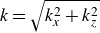 $k = \sqrt {k_x^2 + k_z^2}$
, imposing an exponential decay of the form
$k = \sqrt {k_x^2 + k_z^2}$
, imposing an exponential decay of the form ${\rm e}^{-k y^\prime }$
(Kraichnan Reference Kraichnan1956). As shown in figure 19, the influence on the wall-pressure fluctuations decreases as the source moves away from the wall, and depends on the dimensionless wavenumber
${\rm e}^{-k y^\prime }$
(Kraichnan Reference Kraichnan1956). As shown in figure 19, the influence on the wall-pressure fluctuations decreases as the source moves away from the wall, and depends on the dimensionless wavenumber $kh$
. Although the source terms in bubbly flows are stronger than those in the single-phase flow within the channel core, their contributions to the wall-pressure fluctuations are substantially attenuated with the increasing distance from the wall owing to the associated exponential decay rate. This explains why the pressure fluctuations exhibit significant discrepancies in the channel core, yet the differences appear less pronounced in the 2-D spectra, remain insignificant in the 1-D spectra and become minimal in the wall value of
$kh$
. Although the source terms in bubbly flows are stronger than those in the single-phase flow within the channel core, their contributions to the wall-pressure fluctuations are substantially attenuated with the increasing distance from the wall owing to the associated exponential decay rate. This explains why the pressure fluctuations exhibit significant discrepancies in the channel core, yet the differences appear less pronounced in the 2-D spectra, remain insignificant in the 1-D spectra and become minimal in the wall value of $p^\prime _{\textit{rms}}$
. Nevertheless, the 2-D spectra are still able to capture the essential characteristics of wall-pressure fluctuations that are induced by bubbles.
$p^\prime _{\textit{rms}}$
. Nevertheless, the 2-D spectra are still able to capture the essential characteristics of wall-pressure fluctuations that are induced by bubbles.
6. Conclusions
In this paper the spatio-temporal characteristics of pressure fluctuations of bubbly channel flows without gravity under high gas volume fractions (up to 11.31 %) are investigated based on LES results, at friction Reynolds numbers $\textit{Re}_\tau = 524{\sim} 546$
– the highest achieved to date to the best of our knowledge.
$\textit{Re}_\tau = 524{\sim} 546$
– the highest achieved to date to the best of our knowledge.
The pressure fluctuation in a bubbly channel flow was analysed using a decomposition based on the variable-density pressure fluctuation Poisson equation. Compared with single-phase turbulence, both the rapid $p'_r$
and slow
$p'_r$
and slow $p'_s$
pressure fluctuation components remain significant in the channel core of bubbly flows. In particular, the intensity of the rapid-linear source term exceeds that of the slow-nonlinear term in the channel core. This behaviour originates from the combined effect of the mean velocity gradients and the mean density gradient generated by bubble motion. The variable-density source associated with density fluctuation, resulting from the sharp density variation at the bubble interface, also plays an important role in the generation of pressure fluctuations. Besides, the surface-tension-induced pressure fluctuation
$p'_s$
pressure fluctuation components remain significant in the channel core of bubbly flows. In particular, the intensity of the rapid-linear source term exceeds that of the slow-nonlinear term in the channel core. This behaviour originates from the combined effect of the mean velocity gradients and the mean density gradient generated by bubble motion. The variable-density source associated with density fluctuation, resulting from the sharp density variation at the bubble interface, also plays an important role in the generation of pressure fluctuations. Besides, the surface-tension-induced pressure fluctuation $p'_{\sigma }$
is a significant contributor to the elevated pressure fluctuation level
$p'_{\sigma }$
is a significant contributor to the elevated pressure fluctuation level $p'_{\textit{rms}}$
in bubbly flows since it is the origin of Laplace pressure across the bubble interface. In contrast, the viscous term
$p'_{\textit{rms}}$
in bubbly flows since it is the origin of Laplace pressure across the bubble interface. In contrast, the viscous term $S_v$
is found to be minimal throughout the domain. Overall, the results indicate that pressure fluctuations in bubbly channel flows arise from the combined effects of bubble-induced density variations, especially the interfacial jump of density, and surface-tension forces between the gas and liquid phases. The study therefore advances theoretical focus from incompressible flow source contributions to variable-density source contributions in turbulent bubbly flows.
$S_v$
is found to be minimal throughout the domain. Overall, the results indicate that pressure fluctuations in bubbly channel flows arise from the combined effects of bubble-induced density variations, especially the interfacial jump of density, and surface-tension forces between the gas and liquid phases. The study therefore advances theoretical focus from incompressible flow source contributions to variable-density source contributions in turbulent bubbly flows.
The influence of bubbles on wall-pressure fluctuations is revealed in the 2-D wavenumber–frequency spectrum $\varPhi _{p^\prime p^\prime }(k_x, \omega )$
. Although the bubbles mainly accumulate in the channel core, they affect the wall-pressure fluctuations. A distinct convection ridge is closely related to the distance between the bubble and wall. The cross-correlation
$\varPhi _{p^\prime p^\prime }(k_x, \omega )$
. Although the bubbles mainly accumulate in the channel core, they affect the wall-pressure fluctuations. A distinct convection ridge is closely related to the distance between the bubble and wall. The cross-correlation $\varPhi _{p^\prime H}(k_x, \omega )$
confirms that this ridge, observed in high gas volume fractions, originates from the transport of bubbles in the near-wall region. Beyond the wavenumber scale related to bubble size, the bubble convection ridge overwhelms the turbulence convection ridge in amplitude and becomes the dominant feature at high gas volume fractions. The convection velocity associated with the bubble ridge remains nearly constant across wavenumbers and frequencies, while the bulk convection velocity of the turbulent bubbly channel flows increases with the gas volume fraction. This finding suggests that bubbly flow may generate narrowband wall-pressure fluctuations, potentially inducing structural vibration at resonant frequencies.
$\varPhi _{p^\prime H}(k_x, \omega )$
confirms that this ridge, observed in high gas volume fractions, originates from the transport of bubbles in the near-wall region. Beyond the wavenumber scale related to bubble size, the bubble convection ridge overwhelms the turbulence convection ridge in amplitude and becomes the dominant feature at high gas volume fractions. The convection velocity associated with the bubble ridge remains nearly constant across wavenumbers and frequencies, while the bulk convection velocity of the turbulent bubbly channel flows increases with the gas volume fraction. This finding suggests that bubbly flow may generate narrowband wall-pressure fluctuations, potentially inducing structural vibration at resonant frequencies.
The present work provides a foundation for understanding the complex interplay among bubbles, turbulence and pressure fluctuations in bubbly flows, and may inform the development of improved turbulence modelling and sound-induced vibration prediction strategies for a wide range of applications. It should also be noted that the current results provide only the mean-square values of the source terms in the Poisson equation, which reflect the overall intensity of each term; the wavenumber–frequency distributions of individual sources remain unresolved, and their specific contributions to wall-pressure fluctuations require further investigation. Considering the high numerical demands, the very-large-scale turbulent structures in bubbly flows cannot be fully resolved in the present simulations. Further studies extending the parameter space to higher Reynolds numbers, broader bubble-size distributions and varying local volume fractions are essential for a comprehensive understanding of turbulent bubbly flows.
Funding
The authors acknowledge the financial support provided by the National Natural Science Foundation of China (Nos. 92252205, 12572277 and 12521002).
Declaration of interests
The authors report no conflict of interest.
Appendix A. Single-phase turbulent channel flow
A.1. Validation of the numerical method
The DNS results by Lee & Moser (Reference Lee and Moser2015) at $\textit{Re}_\tau = 550$
are used for validating our LES simulations for the single-phase flow. As shown in figure 20(a), the friction Reynolds number reaches a steady state after
$\textit{Re}_\tau = 550$
are used for validating our LES simulations for the single-phase flow. As shown in figure 20(a), the friction Reynolds number reaches a steady state after $t U_b/L_x = 47$
(
$t U_b/L_x = 47$
( $t=1.8\ \textrm {s}$
in the simulation time unit). The average over
$t=1.8\ \textrm {s}$
in the simulation time unit). The average over $tU_b/L_x=47\sim 77$
is 549.6 with a standard deviation of 0.31. Therefore, data during this period are used for subsequent analyses such as average calculation and the period corresponds to approximately 30 flow-through times. The profile of the streamwise velocity is displayed in figure 20(b) and the turbulent statistics are displayed in figure 21. It is evident that the present profiles agree well with the reference DNS result.
$tU_b/L_x=47\sim 77$
is 549.6 with a standard deviation of 0.31. Therefore, data during this period are used for subsequent analyses such as average calculation and the period corresponds to approximately 30 flow-through times. The profile of the streamwise velocity is displayed in figure 20(b) and the turbulent statistics are displayed in figure 21. It is evident that the present profiles agree well with the reference DNS result.
Single-phase channel case SP: (a) time history of the friction Reynolds number $\textit{Re}_\tau$
; (b) profile of the spatio-temporally averaged streamwise velocity
$\textit{Re}_\tau$
; (b) profile of the spatio-temporally averaged streamwise velocity $\langle u \rangle$
.
$\langle u \rangle$
.

Comparisons of the second-order velocity moments between the present single-phase results (solid lines) and the DNS results by Lee & Moser (Reference Lee and Moser2015) (dashed lines).

(a) Isopleths of 2-D wavenumber–frequency spectrum of normalised wall-pressure fluctuations $\textrm {log}_{10}[\varPhi _{p^\prime p^\prime }(k_x,\omega )u_\tau /(\tau _w^2h^2)]$
for case SP. (b) Convection velocity
$\textrm {log}_{10}[\varPhi _{p^\prime p^\prime }(k_x,\omega )u_\tau /(\tau _w^2h^2)]$
for case SP. (b) Convection velocity $U_c(k_x)$
.
$U_c(k_x)$
.

A.2. The wavenumber–frequency spectrum of single-phase turbulent channel flow
The convection ridge is distinctly observable in the 2-D wavenumber–frequency spectrum shown in figure 22, where the slope of the ridge corresponds to the convection velocity of coherent structures in the boundary layer. Here the bulk convection velocity, as defined in (5.10), is $U_{bc}=0.630U_b$
, in line with the prediction by Willmarth & Wooldridge (Reference Willmarth and Wooldridge1962). Figure 22(b) further shows the wavenumber-dependent convection velocities of the wall-pressure fluctuations
$U_{bc}=0.630U_b$
, in line with the prediction by Willmarth & Wooldridge (Reference Willmarth and Wooldridge1962). Figure 22(b) further shows the wavenumber-dependent convection velocities of the wall-pressure fluctuations $U_c(k_x)$
. Except the inconsistency at the smallest wavenumber
$U_c(k_x)$
. Except the inconsistency at the smallest wavenumber $k_x=\varDelta k_x$
due to the finite length of computational domain, the present
$k_x=\varDelta k_x$
due to the finite length of computational domain, the present ${U_c} ( {{k_x}} )$
agrees well with the reference DNS data from Li et al. (Reference Li, Yang, Yang, Wang and He2021) with a decreasing feature as
${U_c} ( {{k_x}} )$
agrees well with the reference DNS data from Li et al. (Reference Li, Yang, Yang, Wang and He2021) with a decreasing feature as $k_x$
increases.
$k_x$
increases.
Isopleths of 3-D wavenumber–frequency spectrum of case SP: (a) ${\varPhi _{p^\prime p^\prime }}( {{k_x},{k_z} = 0,\omega } )$
, (b)
${\varPhi _{p^\prime p^\prime }}( {{k_x},{k_z} = 0,\omega } )$
, (b) ${\varPhi _{p^\prime p^\prime }}( {{k_x},{k_z},\omega h/{U_b } = 9.6})$
. The two spectra are normalised as
${\varPhi _{p^\prime p^\prime }}( {{k_x},{k_z},\omega h/{U_b } = 9.6})$
. The two spectra are normalised as $\textrm {log}_{10}[\varPhi _{p^\prime p^\prime }(k_x,k_z,\omega )u_\tau /(\tau _w^2h^3)]$
. (c) A zoomed-in view of the region around
$\textrm {log}_{10}[\varPhi _{p^\prime p^\prime }(k_x,k_z,\omega )u_\tau /(\tau _w^2h^3)]$
. (c) A zoomed-in view of the region around $(k_x,k_z)=(0,0)$
in (b), which shows the artificial acoustic peak in the red circle.
$(k_x,k_z)=(0,0)$
in (b), which shows the artificial acoustic peak in the red circle.

Figure 23(a) shows the 3-D wavenumber–frequency spectrum ${\varPhi _{p^\prime p^\prime }} ( {{k_x},{k_z} = 0,\omega } )$
. As the frequency
${\varPhi _{p^\prime p^\prime }} ( {{k_x},{k_z} = 0,\omega } )$
. As the frequency $\omega$
increases, the location of the convective peak shifts towards higher
$\omega$
increases, the location of the convective peak shifts towards higher $k_x$
. The contour lines of smaller magnitude do not extend parallelly as
$k_x$
. The contour lines of smaller magnitude do not extend parallelly as $k_x$
decreases to zero. That is to say, for a fixed frequency, as
$k_x$
decreases to zero. That is to say, for a fixed frequency, as $k_x$
decreases from the convective wavenumber to zero, the spectral magnitude initially decreases before slightly increasing at lower streamwise wavenumbers, forming a weak local maximum at the lowest resolved streamwise wavenumber. This local maximum has been identified as an artificial acoustic mode by Choi & Moin (Reference Choi and Moin1990), attributed to a numerical artefact resulting from the periodic boundary condition imposed in the streamwise direction. Similarly, artificial acoustic modes also occur in the spanwise direction but are confined to small spanwise wavenumbers as noted by Yang & Yang (Reference Yang and Yang2022).
$k_x$
decreases from the convective wavenumber to zero, the spectral magnitude initially decreases before slightly increasing at lower streamwise wavenumbers, forming a weak local maximum at the lowest resolved streamwise wavenumber. This local maximum has been identified as an artificial acoustic mode by Choi & Moin (Reference Choi and Moin1990), attributed to a numerical artefact resulting from the periodic boundary condition imposed in the streamwise direction. Similarly, artificial acoustic modes also occur in the spanwise direction but are confined to small spanwise wavenumbers as noted by Yang & Yang (Reference Yang and Yang2022).
In this paper, the spatial average of the wall-pressure fluctuation field is calculated and is found to change over time, resulting in frequency components for the mode at the wavenumbers $(k_x, k_z) = (0, 0)$
. This is the direct cause of the artificial acoustics. Expanding the computational domain can attenuate the variations of the spatial average over time, thus reducing the influence of the artificial acoustics. As shown in figure 23(b), the isopleths of
$(k_x, k_z) = (0, 0)$
. This is the direct cause of the artificial acoustics. Expanding the computational domain can attenuate the variations of the spatial average over time, thus reducing the influence of the artificial acoustics. As shown in figure 23(b), the isopleths of ${\varPhi _{p^\prime p^\prime }} ( {{k_x},{k_z},\omega = \omega _0} )$
are closed as ellipse-like curves except for a small region near
${\varPhi _{p^\prime p^\prime }} ( {{k_x},{k_z},\omega = \omega _0} )$
are closed as ellipse-like curves except for a small region near $(k_x, k_z) = (0, 0)$
, similar to those in Yang & Yang (Reference Yang and Yang2022). It is observed that the artificial acoustic modes affect only a small region, marked by the red circle in figure 23(c). The convection peak is located at the yellow, largest magnitude area in figures 23(b) and 23(c). The influence of artificial acoustics on the wavenumber–frequency spectrum of wall-pressure fluctuations near the convection line is acceptable.
$(k_x, k_z) = (0, 0)$
, similar to those in Yang & Yang (Reference Yang and Yang2022). It is observed that the artificial acoustic modes affect only a small region, marked by the red circle in figure 23(c). The convection peak is located at the yellow, largest magnitude area in figures 23(b) and 23(c). The influence of artificial acoustics on the wavenumber–frequency spectrum of wall-pressure fluctuations near the convection line is acceptable.
Appendix B. Influence of viscosity
This appendix examines the sensitivity of the present results to viscosity-related modelling aspects. Two types of viscosity are involved in the simulations: the turbulent viscosity introduced by the LES model and the viscosity contrast across the gas–liquid interface.
B.1. Influence of the LES model in bubbly channel flow
The present work employs a LES framework with the WALE model. The objective is to balance computational cost by relaxing the grid requirement near the wall while refining the grid around the bubbles. To quantify the influence of the WALE model under the present grid resolution, we examine both the magnitude of the modelled turbulent viscosity and the resulting SGS stresses.
As shown in figure 24(a), the time- and space-averaged turbulent kinematic viscosity $\langle \nu _t \rangle$
remains below
$\langle \nu _t \rangle$
remains below $0.08\,\nu _l$
throughout the channel. Local enhancements of
$0.08\,\nu _l$
throughout the channel. Local enhancements of $\nu _t$
occur in regions of strong velocity gradients, such as near the wall and in the vicinity of the gas–liquid interface. However, even in these locally enhanced regions, the instantaneous ratio
$\nu _t$
occur in regions of strong velocity gradients, such as near the wall and in the vicinity of the gas–liquid interface. However, even in these locally enhanced regions, the instantaneous ratio $\nu _t/\nu _m$
remains moderate and is below 0.5, indicating that the eddy viscosity does not dominate the effective viscosity field.
$\nu _t/\nu _m$
remains moderate and is below 0.5, indicating that the eddy viscosity does not dominate the effective viscosity field.
(a) Profiles of the spatio-temporally averaged turbulent kinematic viscosity. (b) Wall-normal distributions of the spatio-temporally averaged shear SGS stresses.

The wall-normal distributions of the mean SGS stresses, normalised by $\rho _l u_\tau ^2$
, show that the shear component remains below
$\rho _l u_\tau ^2$
, show that the shear component remains below $1.5\times 10^{-3}$
(figure 24
b), while the normal components remain even smaller, below
$1.5\times 10^{-3}$
(figure 24
b), while the normal components remain even smaller, below $1\times 10^{-4}$
throughout the channel (figures omitted for brevity). In contrast, the resolved Reynolds stresses are of order unity with the same normalisation (see figure 3
a). This demonstrates that the SGS contribution is several orders of magnitude smaller than the characteristic turbulent stress.
$1\times 10^{-4}$
throughout the channel (figures omitted for brevity). In contrast, the resolved Reynolds stresses are of order unity with the same normalisation (see figure 3
a). This demonstrates that the SGS contribution is several orders of magnitude smaller than the characteristic turbulent stress.
To further assess the impact of the SGS model, additional simulations were performed for cases B64D3 and B128D3 with the SGS model deactivated on the same grid (i.e. uDNS). The inclusion of the WALE model does not produce observable modifications of the interfacial vortical structures or wake development. The bubble-induced convection ridge discussed in the main text remains unchanged. Moreover, the distribution of the gas volume fraction, mean velocity profiles, second-order velocity moments and Reynolds stresses exhibit essentially identical behaviour between LES and uDNS. For clarity, the figures shown in this appendix only present the comparison of second-order velocity moments between B128D3 and B128D3uDNS (see figure 25).
The spectra of wall-pressure fluctuations obtained from LES and uDNS show very good agreement over the entire wavenumber range (see figure 26). This indicates that the pressure fluctuation dynamics is well captured by the resolved scales under the present grid resolution. In particular, the energy-containing range associated with the large-scale turbulent structures and bubble-induced motions discussed in the main text is essentially identical in LES and uDNS, confirming that the inclusion of the WALE model does not alter the principal conclusions of the present study.
Profiles of the second-order velocity moments (solid lines) and Reynolds stresses (dashed lines) for B128D3, B128D3uDNS and B128D3HM (the case using harmonic mean viscosity).

One-dimensional spectra of wall-pressure fluctuations with respect to (a) the streamwise wavenumber $k_x$
, (b) the spanwise wavenumber
$k_x$
, (b) the spanwise wavenumber $k_z$
and (c) frequency
$k_z$
and (c) frequency $\omega$
.
$\omega$
.

B.2. Influence of viscosity contrast across the interface
The treatment of viscosity contrast in multiphase flows has recently been discussed by Toutant (Reference Toutant2025) and Magnaudet et al. (Reference Magnaudet, Bruhier, Mer and Bonometti2025). These studies emphasised that special care is required when constructing viscous stresses near interfaces to ensure the continuity of the viscous stress tensor across the grid cell containing the interface. In particular, their formulations involve identifying the interface normal direction and constructing the stress–strain relation accordingly: arithmetic averaging is used in the normal direction to maintain stress continuity, while harmonic averaging is applied in the tangential directions. Implementing this formulation consistently within the present solver is technically challenging, as it requires a robust identification of the interface normal at the discretisation level and an anisotropic treatment of the viscous operator aligned with the interface orientation. Instead, we conducted a sensitivity test by replacing the arithmetic mean viscosity used in the baseline simulations with a harmonic mean viscosity, ${\mu _m} = {{\mu _l}{\mu _g}}/ [{ ( {1 - {\alpha _l}} ){\mu _l} + {\alpha _l}{\mu _g}}]$
. The related simulation was performed by uDNS for case B128D3 using this formulation, denoted by B128D3HM.
${\mu _m} = {{\mu _l}{\mu _g}}/ [{ ( {1 - {\alpha _l}} ){\mu _l} + {\alpha _l}{\mu _g}}]$
. The related simulation was performed by uDNS for case B128D3 using this formulation, denoted by B128D3HM.
The volume fraction distribution and mean velocity profiles remain unchanged between B128D3 and B128D3HM (figures omitted for brevity). The Reynolds stresses are also nearly identical (see figure 25), indicating that the global turbulent momentum transport is essentially unaffected by the change in viscosity interpolation. In contrast, the second-order velocity moments in B128D3HM are larger than those in B128D3. Since the Reynolds shear stress remains unchanged and the viscosity in the pure gas region is the same between B128D3HM and B128D3, the enhancement in the second-order velocity moment mainly reflects stronger velocity fluctuations in the gas–liquid mixing region. A similar behaviour was reported by Mangani et al. (Reference Mangani, Soligo, Roccon and Soldati2022), who showed that reducing the gas viscosity enhances velocity fluctuations inside the bubbles. The harmonic averaging used here produces a lower effective viscosity in the interfacial region, thereby reducing viscous damping and allowing stronger local velocity fluctuations. According to (4.6) and (4.7), the quantities of Reynolds stress and viscous stress, rather than the second-order velocity moments, contribute to the pressure fluctuations. More broadly, previous simulations of bubbly channel flows have employed a wide range of liquid–gas viscosity ratios and interpolation strategies without reporting substantial changes in the global momentum balance (Lu et al. Reference Lu, Yang and Deng2025). Therefore, we may safely use the volume-fraction-weighted approach to calculate the mixture properties.
To further verify this conclusion concerning pressure fluctuations, the wall-pressure fluctuation spectra obtained from B128D3HM and B128D3 exhibit excellent collapse across the resolved wavenumber/frequency range in figure 26, suggesting that the pressure fluctuation dynamics is essentially insensitive to the treatment of viscosity interpolation.
Appendix C. Validation of computational domain size
Considering computational resource constraints, the current domain size represents a balanced compromise. The adequacy of the domain size is validated by the two-point correlation coefficients of the velocity field, as shown in figure 27. The two-point correlation coefficients are defined as
 \begin{align} \begin{aligned} {R_{\phi \phi }} ( \xi ,y )=\frac {{\langle {\phi (x,y,z,t)\phi (x + \xi ,y,z,t)} \rangle }}{{\langle {{\phi }^2}\rangle }},\quad {R_{\phi \phi }} ( \zeta ,y )=\frac {{\langle {\phi (x,y,z,t)\phi (x,y,z+\zeta ,t)} \rangle }}{{\langle {{\phi }^2}\rangle }}. \end{aligned} \end{align}
When the separation distance approaches the domain length in either the streamwise ( $\xi \rightarrow L_x$
) or spanwise (
$\xi \rightarrow L_x$
) or spanwise ( $\zeta \rightarrow L_z$
) direction, the correlation coefficients decay to nearly zero, indicating that the present domain size is sufficient to capture the coherent turbulent structures. In addition to the near-wall results at
$\zeta \rightarrow L_z$
) direction, the correlation coefficients decay to nearly zero, indicating that the present domain size is sufficient to capture the coherent turbulent structures. In addition to the near-wall results at $y^+=10$
, the two-point correlations at the channel-centre plane of case B128D3 (
$y^+=10$
, the two-point correlations at the channel-centre plane of case B128D3 ( $y/h=1$
,
$y/h=1$
, $y^+=530$
) also exhibit a clear decay. Even in the region where the gas volume fraction is relatively high, the velocity fluctuations still decorrelate within the present domain. In this regard, the present computational domain size of
$y^+=530$
) also exhibit a clear decay. Even in the region where the gas volume fraction is relatively high, the velocity fluctuations still decorrelate within the present domain. In this regard, the present computational domain size of $L_x \times L_y \times L_z = 4h \times 2h \times 2h$
, although smaller than those in some DNS studies (see table 1), is considered adequate for the phenomena considered in this study.
$L_x \times L_y \times L_z = 4h \times 2h \times 2h$
, although smaller than those in some DNS studies (see table 1), is considered adequate for the phenomena considered in this study.
Appendix D. Mesh resolution tests for bubbly channel flow
The fundamental requirement of mesh resolution for bubbles comes from the interface and the vorticity produced at the bubble surface, which depends on the bubble Reynolds number (Riboux et al. Reference Riboux, Legendre and Risso2013). In the present work, the magnitude of the local slip velocity between the liquid and gas phases is defined as ${U_{{\textit{rel}}}} ( y ) = \left | {\langle {u_l}\rangle ( y ) - \langle {u_g}\rangle ( y )} \right |$
. The maximum value of this quantity across the channel height satisfies
${U_{{\textit{rel}}}} ( y ) = \left | {\langle {u_l}\rangle ( y ) - \langle {u_g}\rangle ( y )} \right |$
. The maximum value of this quantity across the channel height satisfies $\mathop {\max }_y \left \{ {{U_{{\textit{rel}}}} ( y )} \right \} \lt 0.1 U_b$
. To estimate a representative bubble Reynolds number, we further define a bulk slip velocity by averaging
$\mathop {\max }_y \left \{ {{U_{{\textit{rel}}}} ( y )} \right \} \lt 0.1 U_b$
. To estimate a representative bubble Reynolds number, we further define a bulk slip velocity by averaging $U_{\textit{rel}}(y)$
over the wall-normal region where the gas phase is statistically present. Specifically,
$U_{\textit{rel}}(y)$
over the wall-normal region where the gas phase is statistically present. Specifically, $y_1$
and
$y_1$
and $y_2$
denote the lower and upper bounds of the region satisfying
$y_2$
denote the lower and upper bounds of the region satisfying $\langle \alpha _g \rangle \gt 0.001$
, and
$\langle \alpha _g \rangle \gt 0.001$
, and ${U_{{\textit{rel,b}}}} = ({1}/({y_1-y_2})) \int _{y_1}^{y_2} {{U_{{\textit{rel}}}} ( y ){\mathrm{d}}y}$
. The corresponding bubble Reynolds number is then estimated as
${U_{{\textit{rel,b}}}} = ({1}/({y_1-y_2})) \int _{y_1}^{y_2} {{U_{{\textit{rel}}}} ( y ){\mathrm{d}}y}$
. The corresponding bubble Reynolds number is then estimated as $\textit{Re}_b = U_{{\textit{rel,b}}} D_b/ \nu _l \lt 50$
(see table 4). Under this situation, bubbles roughly follow the carrier-phase motion and wake structures are relatively weak, momentum transport is primarily governed by inertia and phase distribution.
$\textit{Re}_b = U_{{\textit{rel,b}}} D_b/ \nu _l \lt 50$
(see table 4). Under this situation, bubbles roughly follow the carrier-phase motion and wake structures are relatively weak, momentum transport is primarily governed by inertia and phase distribution.
The bulk absolute gas–liquid slip velocity $U_{{\textit{rel,b}}}$
and corresponding bubble Reynolds number
$U_{{\textit{rel,b}}}$
and corresponding bubble Reynolds number $\textit{Re}_{\textit{b}}$
for bubbly cases.
$\textit{Re}_{\textit{b}}$
for bubbly cases.

Two-point correlation coefficients of velocity fluctuations for SP on the plane at $y^+ = 10$
(a,b) and B128D3 on the plane at
$y^+ = 10$
(a,b) and B128D3 on the plane at $y^+ = 10$
(solid lines) and
$y^+ = 10$
(solid lines) and $y^+ = 530$
(dashed lines) (c,d). (a,c) Streamwise direction, (b,d) spanwise direction.
$y^+ = 530$
(dashed lines) (c,d). (a,c) Streamwise direction, (b,d) spanwise direction.

Profiles of (a) the spatio-temporally averaged gas volume fraction $\langle \alpha _g \rangle$
, and (b) the spatio-temporally averaged streamwise velocity of case B64D2 under different mesh resolutions. Notation ‘R30’, for example, denotes a mesh with
$\langle \alpha _g \rangle$
, and (b) the spatio-temporally averaged streamwise velocity of case B64D2 under different mesh resolutions. Notation ‘R30’, for example, denotes a mesh with $D_b/\varDelta _x = D_b/\varDelta _z = 30$
and
$D_b/\varDelta _x = D_b/\varDelta _z = 30$
and $D_b/\varDelta _y \geqslant 30$
over the channel centre.
$D_b/\varDelta _y \geqslant 30$
over the channel centre.

Profiles of the second-order velocity moments of case B64D2 under different mesh resolutions.

The grid used in this study features equal streamwise and spanwise resolutions ( $\varDelta _x = \varDelta _z \equiv \varDelta$
), with a uniform expansion ratio applied in the wall-normal direction (see table 2). The mesh convergence tests begin with a resolution of
$\varDelta _x = \varDelta _z \equiv \varDelta$
), with a uniform expansion ratio applied in the wall-normal direction (see table 2). The mesh convergence tests begin with a resolution of $D_b/\varDelta \approx 20$
for the 2 mm bubbles, and subsequently refined to
$D_b/\varDelta \approx 20$
for the 2 mm bubbles, and subsequently refined to $D_b/\varDelta \approx 26$
, 30 and 36. As shown in figure 28(a), the gas volume fraction distribution for the coarsest mesh (
$D_b/\varDelta \approx 26$
, 30 and 36. As shown in figure 28(a), the gas volume fraction distribution for the coarsest mesh ( $D_b/\varDelta = 20$
) exhibits excessive accumulation near the channel centre, whereas the results with finer meshes (
$D_b/\varDelta = 20$
) exhibits excessive accumulation near the channel centre, whereas the results with finer meshes ( $D_b/\varDelta \approx 26$
, 30 and 36) show good agreement and convergence.
$D_b/\varDelta \approx 26$
, 30 and 36) show good agreement and convergence.
In addition to the convergence of the gas volume fraction, figure 28(b) shows the profiles of the mean streamwise velocity, while figure 29 presents the second-order velocity moments obtained with different mesh resolutions. For meshes with $D_b/\varDelta \gtrsim 26$
, both the mean velocity profiles and the second-order moments show good agreement, indicating satisfactory convergence. Among the second-order statistics, the wall-normal velocity variance
$D_b/\varDelta \gtrsim 26$
, both the mean velocity profiles and the second-order moments show good agreement, indicating satisfactory convergence. Among the second-order statistics, the wall-normal velocity variance $\langle v'v' \rangle$
is found to be the most sensitive to mesh resolution. For the coarsest mesh (B64D2R20),
$\langle v'v' \rangle$
is found to be the most sensitive to mesh resolution. For the coarsest mesh (B64D2R20), $\langle v'v' \rangle$
is significantly overestimated in the core region of the channel (
$\langle v'v' \rangle$
is significantly overestimated in the core region of the channel ( $y\gt 0.8h$
) compared with the finer meshes. Based on these observations, a minimum resolution of approximately 26 cells per bubble diameter is required to reliably capture the bubble-induced velocity fluctuations, particularly the wall-normal velocity variance. For bubbly flows with
$y\gt 0.8h$
) compared with the finer meshes. Based on these observations, a minimum resolution of approximately 26 cells per bubble diameter is required to reliably capture the bubble-induced velocity fluctuations, particularly the wall-normal velocity variance. For bubbly flows with $\textit{Re}_b = 50$
–236 investigated by du Cluzeau et al. (Reference du Cluzeau, Bois and Toutant2019), a resolution of
$\textit{Re}_b = 50$
–236 investigated by du Cluzeau et al. (Reference du Cluzeau, Bois and Toutant2019), a resolution of $D_b/\varDelta = 12.8$
–25.6 yields uncertainties below 10 % relative to experiments and within 5 % compared with infinitely refined mesh extrapolation. For higher bubble Reynolds numbers, e.g.
$D_b/\varDelta = 12.8$
–25.6 yields uncertainties below 10 % relative to experiments and within 5 % compared with infinitely refined mesh extrapolation. For higher bubble Reynolds numbers, e.g. $\textit{Re}_b = 438$
, a finer resolution of
$\textit{Re}_b = 438$
, a finer resolution of $D_b/\varDelta \sim 25$
–55 is required to accurately capture both first- and second-order statistics (du Cluzeau et al. Reference du Cluzeau, Bois, Leoni and Toutant2022). Based on these assessments and other cases listed in table 1, it can be qualitatively estimated that
$D_b/\varDelta \sim 25$
–55 is required to accurately capture both first- and second-order statistics (du Cluzeau et al. Reference du Cluzeau, Bois, Leoni and Toutant2022). Based on these assessments and other cases listed in table 1, it can be qualitatively estimated that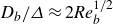 $D_b /\varDelta \approx 2 \textit{Re}_b^{1/2}$
in terms of boundary layer thickness (Riboux et al. Reference Riboux, Legendre and Risso2013), serving as an average criterion.
$D_b /\varDelta \approx 2 \textit{Re}_b^{1/2}$
in terms of boundary layer thickness (Riboux et al. Reference Riboux, Legendre and Risso2013), serving as an average criterion.
Combined with the surface Weber number criterion discussed in § 2.2, the present simulations adopt a mesh resolution satisfying $D_b/\varDelta \gt 30 \approx 4 \textit{Re}_b^{1/2}$
. This choice offers a conservative margin above the identified threshold.
$D_b/\varDelta \gt 30 \approx 4 \textit{Re}_b^{1/2}$
. This choice offers a conservative margin above the identified threshold.
Profiles of (a) the gas volume fraction $\langle \alpha _g \rangle$
, and (b) the streamwise velocity
$\langle \alpha _g \rangle$
, and (b) the streamwise velocity $\langle u \rangle$
of case B128D3 obtained using different averaging intervals. The averaging duration is expressed in flow-through times
$\langle u \rangle$
of case B128D3 obtained using different averaging intervals. The averaging duration is expressed in flow-through times $L_x/U_b$
. Solid lines show data from the lower half-channel (
$L_x/U_b$
. Solid lines show data from the lower half-channel ( $y/h\in [0,1]$
), while dashed lines represent the mirror-symmetric extension of results from the upper half-channel (
$y/h\in [0,1]$
), while dashed lines represent the mirror-symmetric extension of results from the upper half-channel ( $y/h\in [1,2]$
).
$y/h\in [1,2]$
).

Appendix E. Validation of statistically stationary state
The statistical convergence in time can be judged by examining the symmetry in the distributions of characteristic quantities (Cifani et al. Reference Cifani, Kuerten and Geurts2020). In this section we assess the wall-normal distributions of the mean gas volume fraction, mean streamwise velocity, second-order velocity moments and Reynolds stresses for different averaging durations, taking case B128D3 as a representative example. The results are shown in figures 30, 31 and 32.
As the averaging duration increases from $12.95\,L_x/U_b$
to
$12.95\,L_x/U_b$
to $38.86\,L_x/U_b$
, the overall distributions remain consistent while noticeable reductions in inter-side discrepancies and profile fluctuations can be observed. Both the magnitude of local variations and the asymmetry between the upper and lower channel halves decrease progressively, indicating gradual statistical convergence. The profiles obtained at
$38.86\,L_x/U_b$
, the overall distributions remain consistent while noticeable reductions in inter-side discrepancies and profile fluctuations can be observed. Both the magnitude of local variations and the asymmetry between the upper and lower channel halves decrease progressively, indicating gradual statistical convergence. The profiles obtained at $38.86\,L_x/U_b$
exhibit stable distributions with good symmetry and are therefore adopted in the present analysis.
$38.86\,L_x/U_b$
exhibit stable distributions with good symmetry and are therefore adopted in the present analysis.
The secondary peak in the volume fraction distribution is already clearly identifiable at an averaging duration of $12.95\,L_x/U_b$
. Its wall-normal location and magnitude remain essentially unchanged as the averaging duration increases to
$12.95\,L_x/U_b$
. Its wall-normal location and magnitude remain essentially unchanged as the averaging duration increases to $38.86\,L_x/U_b$
, and the peak persists even when the averaging duration is extended to approximately three times
$38.86\,L_x/U_b$
, and the peak persists even when the averaging duration is extended to approximately three times $38.86\,L_x/U_b$
. This persistence indicates that the secondary peak is a robust and sustained feature of the flow rather than an artefact of limited temporal sampling.
$38.86\,L_x/U_b$
. This persistence indicates that the secondary peak is a robust and sustained feature of the flow rather than an artefact of limited temporal sampling.
Figure 33 further illustrates the statistical symmetry of the volume fraction profile at an averaging duration of $38.86\,L_x/U_b$
for all bubbly cases, where the distributions from the two channel halves closely overlap. All results presented in this paper are therefore computed using this averaging duration.
$38.86\,L_x/U_b$
for all bubbly cases, where the distributions from the two channel halves closely overlap. All results presented in this paper are therefore computed using this averaging duration.
Profiles of second-order velocity moments of case B128D3 obtained under different averaging durations. The legends are the same as those in figure 30.

Profiles of Reynolds stresses for case B128D3 under different averaging durations. The legends are the same as those in figure 30.

Comparison of gas volume fraction profiles between the lower and upper halves of the channel at an averaging duration of $38.86\,L_x/U_b$
.
$38.86\,L_x/U_b$
.


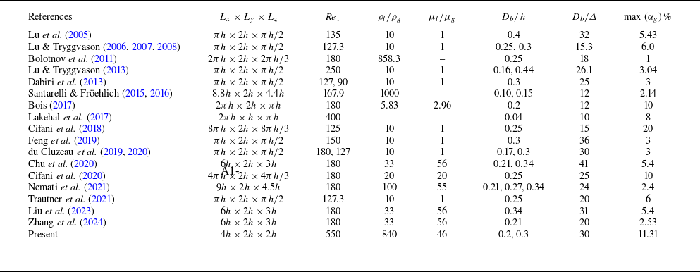
 Lx×Ly×Lz
 Reτ
Reτ ρl/ρg
ρl/ρg μl/μg
μl/μg Db/h
Db/h Db/Δ
Db/Δ αg¯
αg¯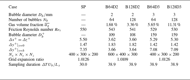
 h=0.01
 p′
p′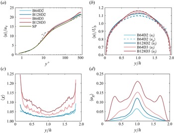
 ⟨u⟩+
⟨u⟩+ u+=y+
u+=y+ u+=(1/κ)lny++B
 κ=0.4
κ=0.4 B=5.5
B=5.5 ⟨ul⟩=⟨αl⋅u⟩/⟨α⟩
 ⟨ug⟩=⟨αg⋅u⟩/⟨αg⟩
 χ
χ ⟨αg⟩
⟨αg⟩
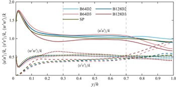
 ⟨u′u′⟩/k
 ⟨v′v′⟩/k
 ⟨w′w′⟩/k

 ⟨p⟩
⟨p⟩ −⟨v′v′⟩
 prms′=⟨p′2¯⟩
 prms′
prms′ Ubc/Ub
 p′
p′ pr′+ps′
 pr′
pr′ ps′
ps′ y/h=0.1
 z/h=0.1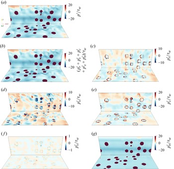
 p′
p′ pr′+ps′+pc′+pv′+pσ′
 pr′
pr′ ps′
ps′ pc′
pc′ pv′
pv′ pσ′
pσ′ y/h=0.5
 z
z z/h=0.1
 ∇2p′
∇2p′ Sr
Sr Ss
Ss Sc
Sc Sv
Sv Sσ
Sσ y/h=0.5
 z
z z/h=0.1


 Φp′p′(kx,ω)
 Ubc=ω/kx
 kx
kx ω
ω Φp′p′(kx∗,ω)
 Φp′p′(kx,ω∗)
 log10[Φp′p′(kx,ω)uτ/(τw2h2)]
 Φp′H(kx,ω)
 Φp′p′(kx∗,ω)
 kx∗h=27,35,50
 Q
Q Q=7×10⁴
 y+=30
y+=30
 log10[Φp′p′(kx,kz)/(τw2h2)]
 Uc(kx)
 Uc(kx)peak
 Ubc/Ub
 kx
kx kz
kz ω
ω kxDb
kxDb kzDb
kzDb Db=2 and 3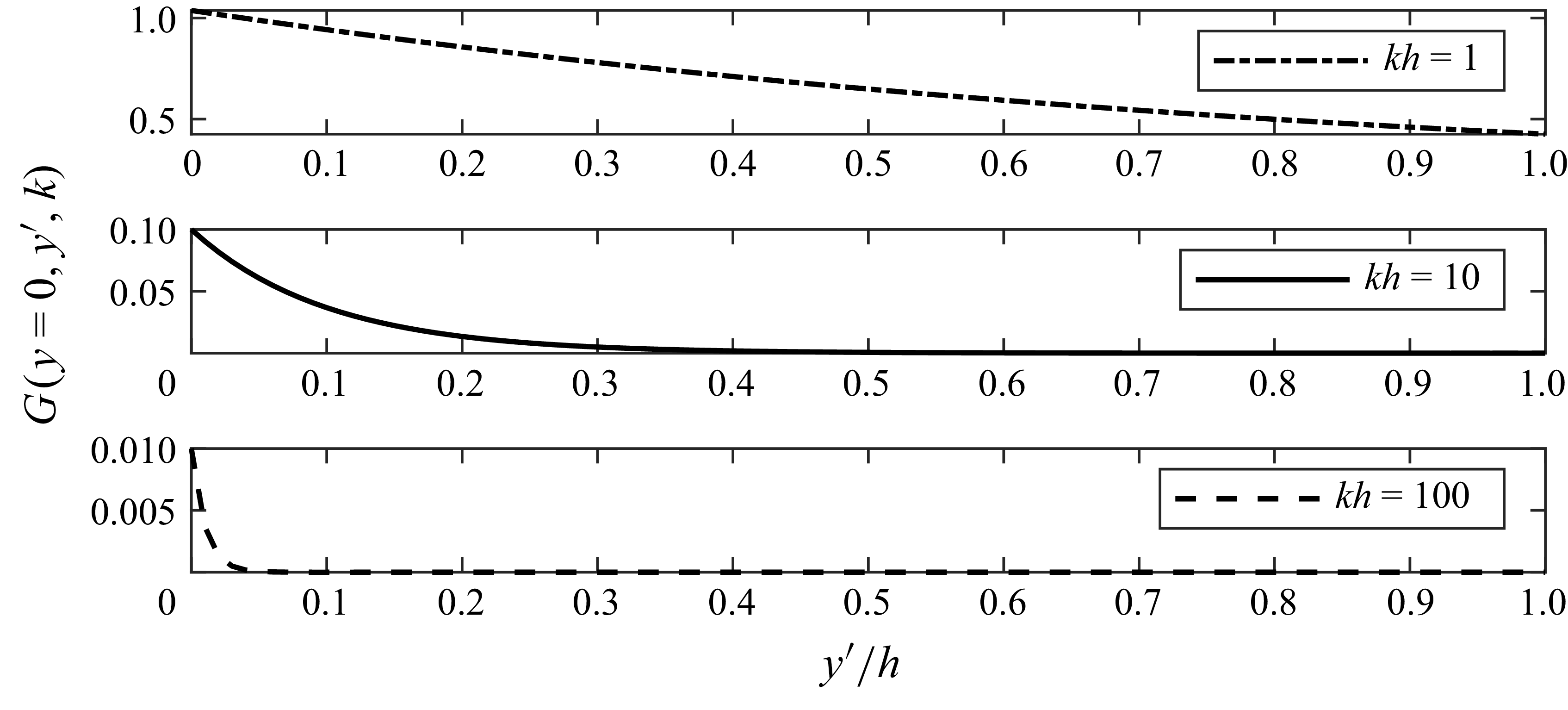
 G(y=0,y′,k)
 kh
kh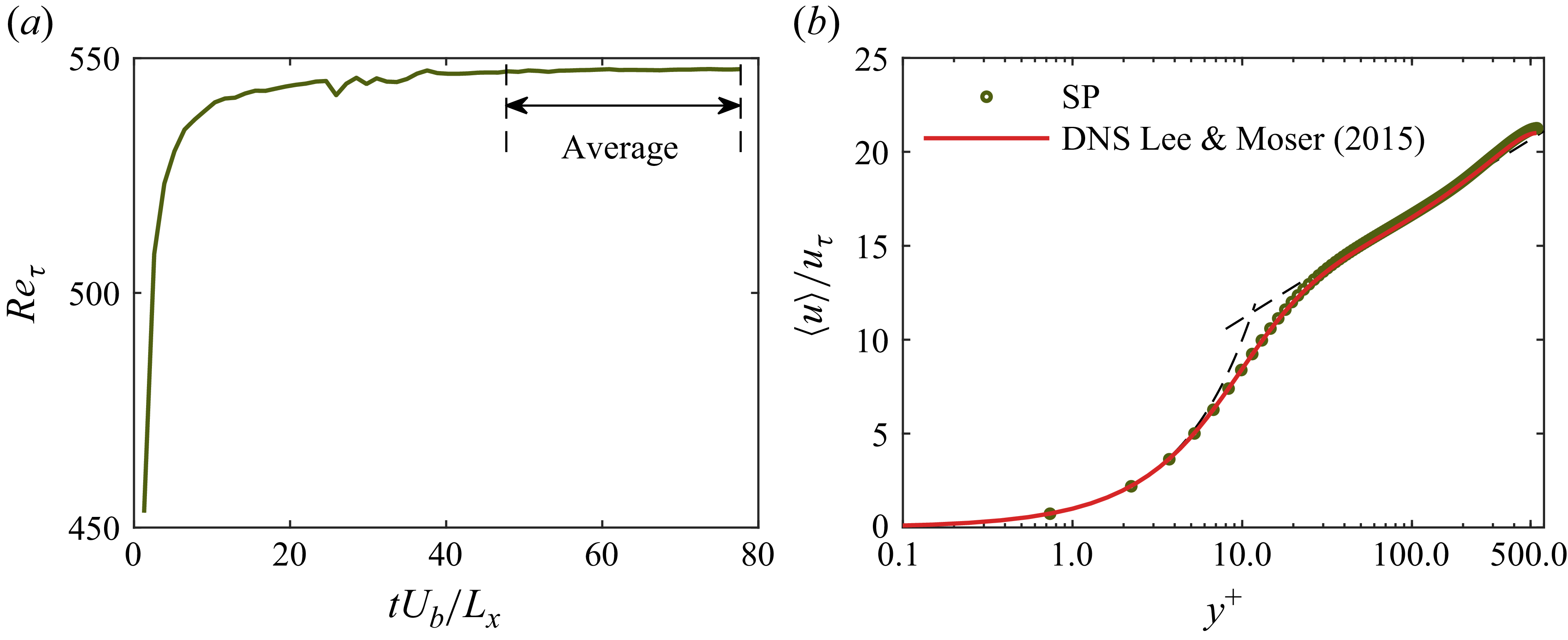
 Reτ
Reτ ⟨u⟩
⟨u⟩
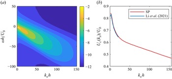
 log10[Φp′p′(kx,ω)uτ/(τw2h2)]
 Uc(kx)
 Φp′p′(kx,kz=0,ω)
 Φp′p′(kx,kz,ωh/Ub=9.6)
 log10[Φp′p′(kx,kz,ω)uτ/(τw2h3)]
 (kx,kz)=(0,0)


 kx
kx kz
kz ω
ω
 Urel,b
 Reb
Reb
 y+=10
y+=10 y+=10
y+=10 y+=530
 ⟨αg⟩
⟨αg⟩ Db/Δx=Db/Δz=30
 Db/Δy⩾30

 ⟨αg⟩
⟨αg⟩ ⟨u⟩
⟨u⟩ Lx/Ub
Lx/Ub y/h∈[0,1]
 y/h∈[1,2]
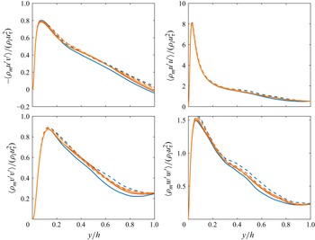

 38.86Lx/Ub

