


1. Introduction
Despite recent progress in high-performance computing, performing large-scale plasma turbulence simulations remains computationally challenging. In particular, the complexities of multi-dimensional, multi-component data, coupled with the strong nonlinear interactions in turbulent fields, often complicate both computational cost and physical interpretation. The key role of numerical simulations in this framework is to perform parametric scans of relevant engineering parameters, thereby accelerating experimental work. However, evolving the complex dynamics in plasma turbulence simulations often requires a significant amount of time to reach a quasi-steady state. It is therefore appealing to complement the evolution of the underlying equations, by leveraging experimental or numerical data, directly in the simulation process. The main advantage of data-driven or data-augmented simulations is that they can replace some of the time-consuming numerical steps – those irrelevant to physical interpretation but necessary to reach the final quasi-steady state – with inferences made directly from data. These data inferences are often much less expensive to generate than performing a complete simulation, potentially leading to significant time savings.
Data-driven methods have been widely used in plasma physics from high-temperature fusion reactors to low-temperature space applications (Anirudh et al. Reference Anirudh2023). A common way to introduce data into the numerical simulation is through reduced or surrogate models. These approaches generally involve the generation of a reduced basis (Quarteroni, Manzoni & Negri Reference Quarteroni, Manzoni and Negri2015; Hesthaven, Rozza & Stamm Reference Hesthaven, Rozza and Stamm2016), often through proper orthogonal decomposition (POD) (Volkwein Reference Volkwein2011), which enables the projection of high-dimensional data onto an optimal low-dimensional space. In particular, the POD efficiently captures lower-order modes in plasma simulations using a very small basis representation (del Castillo-Negrete et al. Reference del Castillo-Negrete, Hirshman, Spong and D’Azevedo2007; Futatani, Benkadda & del Castillo-Negrete Reference Futatani, Benkadda and del Castillo-Negrete2009; Yatomi, Nakata & Sasaki Reference Yatomi, Nakata and Sasaki2024). These low-dimensional representations have been successfully applied in numerical fluid simulations (Ravindran Reference Ravindran2000) and have been applied to simulations of plasma relevant for fusion reactors (Nicolini, Na & Teixeira Reference Nicolini, Na and Teixeira2019; Nicolini & Teixeira Reference Nicolini and Teixeira2021). Additionally, reduced representations can be applied directly to learn a mapping function or operator using neural networks (Hesthaven & Ubbiali Reference Hesthaven and Ubbiali2018; Bhattacharya et al. Reference Bhattacharya, Hosseini, Kovachki and Stuart2021), significantly simplifying the numerical simulation process, thereby reducing computational cost. This approach has also been applied in high-energy plasma physics for various applications including numerical simulations (Nicolini & Teixeira Reference Nicolini and Teixeira2021; Liu et al. Reference Liu, Akcay, Lao and Sun2022), with recent work demonstrating that mixed-fidelity surrogate modelling can speed up large-scale turbulence calculations (Wan Reference Wan2025), recovering equilibrium profiles from experimental data (Lao et al. Reference Lao2022) and predicting plasma detachment (Zhu et al. Reference Zhu, Zhao, Bhatia, Xu, Bremer, Meyer, Li and Rognlien2022).
In this work, we apply a data-driven approach combining model order reduction, based on POD, with deep neural networks to accelerate nonlinear, flux-driven, three-dimensional, two-fluid Global Braginskii Solver (GBS) simulations (Giacomin et al. Reference Giacomin, Ricci, Coroado, Fourestey, Galassi, Lanti, Mancini, Richart, Stenger and Varini2022). To generate comprehensive datasets for model training and validation, we perform a parametric scan of plasma resistivity, heating source and density sources across various turbulent regimes. The dataset is divided into a training dataset, used for model construction, and an independent validation dataset, used for model verification. Our approach consists of two main steps. First, we apply POD to extract an optimal low-dimensional basis from the high-dimensional numerical dataset, significantly reducing computational complexity. Second, we train neural networks to predict plasma states within this reduced basis representation. These machine leaning (ML)-generated states are then used to restart GBS simulations, which evolve to a self-consistent quasi-steady state characterised by density profiles no longer significantly fluctuating between time steps.
To assess the performance of this approach, we consider a single-null (SN) magnetic configuration with a volume approximately corresponding to $1/3$
of the TCV tokamak. We evaluate the performance of the neural network to generate physically consistent quasi-steady-state solutions and validate its accuracy using GBS-generated reference datasets. Additionally, we analyse approximation errors introduced by model order reduction and their impact on model expressiveness. Finally, we assess the computational advantages of ML-assisted simulations by comparing the evolution of key plasma equilibrium properties with standard GBS simulations, demonstrating that ML-generated restarts accelerate convergence to the quasi-steady state by up to a factor of three.
$1/3$
of the TCV tokamak. We evaluate the performance of the neural network to generate physically consistent quasi-steady-state solutions and validate its accuracy using GBS-generated reference datasets. Additionally, we analyse approximation errors introduced by model order reduction and their impact on model expressiveness. Finally, we assess the computational advantages of ML-assisted simulations by comparing the evolution of key plasma equilibrium properties with standard GBS simulations, demonstrating that ML-generated restarts accelerate convergence to the quasi-steady state by up to a factor of three.
The remainder of the paper is structured as follows: § 2 introduces the GBS model used to generate the numerical datasets and describes the model order reduction and ML methods applied to train the neural network. Section 3 evaluates the approximation error introduced by reduced-order modelling, assesses the overall model performance and compares ML-generated plasma profiles with those obtained from GBS simulations. Section 3.4 compares the computational efficiency of ML-generated restarts in comparison with simulations from scratch. Finally, conclusions and future perspectives are discussed in § 4.
2. Numerical model
In this section, we introduce the GBS model used to generate the dataset of boundary plasma turbulence simulations for training and validating ML models. We provide a brief overview of the GBS simulation process, describe the structure of the final dataset and discuss the parametric scan chosen to drive various turbulent regimes in our simulations. Finally, we explain the mathematical description of model order reduction based on POD, as well as the structure of the data-driven neural networks.
2.1. The GBS code
The three-dimensional drift-reduced Braginskii equations (Zeiler et al. Reference Zeiler1997), implemented in the GBS code, simulate the dynamics of both the plasma and neutrals within an extended domain that encompasses both the core and boundary regions (Giacomin et al. Reference Giacomin, Ricci, Coroado, Fourestey, Galassi, Lanti, Mancini, Richart, Stenger and Varini2022). The coordinate system used in the GBS code is independent of the magnetic field, allowing for the study of various alternative divertor configurations (ADCs), such as snowflake (Giacomin, Stenger & Ricci Reference Giacomin, Stenger and Ricci2020), negative triangularity (Lim et al. Reference Lim, Giacomin, Ricci, Coelho, Février, Mancini, Silvagni and Stenger2023), double-null (Lim et al. Reference Lim2024) and non-axisymmetric (Coelho et al. Reference Coelho, Loizu, Ricci and Giacomin2022) configurations.
In the present work, we focus exclusively on the electrostatic case, excluding interactions between plasma and neutrals. Consequently, the GBS model equations are simplified to the following form:
 \begin{align} \frac {\partial n}{\partial t} = -\frac {\rho _*^{-1}}{B}[\phi , n] + \frac {2}{B}[C(p_e)-nC(\phi )]-\boldsymbol{\nabla} _\parallel (nv_{\parallel e}) + D_n {\nabla} ^2_\perp n + s_n, \end{align}
 \begin{align} \frac {\partial \varOmega }{\partial t} = -\frac {\rho _*^{-1}}{B} \boldsymbol{\nabla }\boldsymbol{\cdot }[\phi , \omega ] -\boldsymbol{\nabla }\boldsymbol{\cdot }\big (v_{\parallel i} \boldsymbol{\nabla} _\parallel \omega \big ) + B^2 \boldsymbol{\nabla} _\parallel j_\parallel + 2B C(p_e + \tau p_i) + D_\varOmega {\nabla} _\perp ^2 \varOmega,\end{align}
 \begin{align} \frac {\partial v_{\parallel i}}{\partial t} = -\frac {\rho _*^{-1}}{B}[\phi , v_{\parallel i}]-v_{\parallel i} \boldsymbol{\nabla} _\parallel v_{\parallel i} - \frac {1}{n}\boldsymbol{\nabla} _\parallel (p_e + \tau p_i) + D_{v_{\parallel i}} {\nabla} _\perp ^2 v_{\parallel i},\end{align}
 \begin{align} \frac {\partial v_{\parallel e}}{\partial t} &= -\frac {\rho _*^{-1}}{B}[\phi , v_{\parallel , e}] - v_{\parallel e}\boldsymbol{\nabla} _\parallel v_{\parallel e} + \frac {m_i}{m_e}\Bigg (\nu j_\parallel + \boldsymbol{\nabla} _\parallel \phi -\frac {1}{n}\boldsymbol{\nabla} _\parallel p_e-0.71 \boldsymbol{\nabla} _\parallel T_e \Bigg ) \nonumber \\ & \quad+ D_{v_{\parallel e}}{\nabla} _\perp ^2 v_{\parallel e},\end{align}
 \begin{align} \frac {\partial T_i}{\partial t} &=-\frac {\rho _*^{-1}}{B}[\phi , T_i] - v_{\parallel i}\boldsymbol{\nabla} _\parallel T_i + \frac {4}{3}\frac {T_i}{B}\bigg [C(T_e) + \frac {T_e}{n}C(n)-C(\phi ) \bigg ] -\frac {10}{3}\tau \frac {T_i}{B}C(T_i) \nonumber \\ &\quad + \frac {2}{3}T_i\bigg [(v_{\parallel i}-v_{\parallel e})\frac {\boldsymbol{\nabla} _\parallel n}{n}-T_i \boldsymbol{\nabla} _\parallel v_{\parallel e}\bigg ] + 2.61\nu n (T_e -\tau T_i)+ \boldsymbol{\nabla} _\parallel ( \chi _{\parallel i}\boldsymbol{\nabla} _\parallel T_i) \nonumber \\ &\quad + D_{T_i}{\nabla} _\perp ^2 T_i + s_{T_i},\end{align}
 \begin{align} \frac {\partial T_e}{\partial t} &= -\frac {\rho _*^{-1}}{B}[\phi , T_e] - v_{\parallel e}\boldsymbol{\nabla} _\parallel T_e + \frac {2}{3}T_e\bigg [0.71 \frac {\boldsymbol{\nabla} _\parallel j_\parallel }{n}-\boldsymbol{\nabla} _\parallel v_{\parallel e}\bigg ] -2.61\nu n (T_e-\tau T_i) \nonumber \\ &\quad + \frac {4}{3}\frac {T_e}{B}\bigg [\frac {7}{2}C(T_e)+\frac {T_e}{n}C(n)-C(\phi ) \bigg ] + \boldsymbol{\nabla} _\parallel (\chi _{\parallel e}\boldsymbol{\nabla} _\parallel T_e) + D_{T_e}{\nabla} _\perp ^2 T_e + s_{T_e}. \end{align}
In these equations, $B=\lvert\boldsymbol B \rvert$
is the magnetic-field strength,
$B=\lvert\boldsymbol B \rvert$
is the magnetic-field strength, $\rho_*=\rho_{s0}/R_0$
is the normalized-ion sound Larmor radius,
$\rho_*=\rho_{s0}/R_0$
is the normalized-ion sound Larmor radius, $\phi$
is the electrostatic potential,
$\phi$
is the electrostatic potential, $p_e=n T_e$
and
$p_e=n T_e$
and $p_i=nT_i$
are the electron and ion pressures,
$p_i=nT_i$
are the electron and ion pressures, $C(\cdot)$
is the magnetic-curvature operatore,
$C(\cdot)$
is the magnetic-curvature operatore, $D$
denotes perpendicular diffusion coefficients multiplying the
$D$
denotes perpendicular diffusion coefficients multiplying the $\nabla^2_\perp$
closures,
$\nabla^2_\perp$
closures, $s_n$
and
$s_n$
and $s_T$
denotes the particle and heat source terms (specificed in (2.9) and (2.10)),
$s_T$
denotes the particle and heat source terms (specificed in (2.9) and (2.10)), $\tau=T_{i0}/T_{e0}$
is the ion-to-electron reference temperature ratio, and
$\tau=T_{i0}/T_{e0}$
is the ion-to-electron reference temperature ratio, and $\chi_{\parallel}$
is the parallel thermal conductivity.
$\chi_{\parallel}$
is the parallel thermal conductivity.
These equations are coupled with the Poisson equation, avoiding the Boussinesq approximation:
 \begin{align} \boldsymbol{\nabla }\boldsymbol{\cdot }( n\boldsymbol{\nabla} _\perp \phi) = \varOmega - \tau {\nabla} _\perp ^2 p_i. \end{align}
Here, $\varOmega =\boldsymbol{\nabla }\boldsymbol{\cdot }\omega$
represents the scalar vorticity, where the polarization vector
$\varOmega =\boldsymbol{\nabla }\boldsymbol{\cdot }\omega$
represents the scalar vorticity, where the polarization vector $\omega$
is defined as
$\omega$
is defined as $\omega= \boldsymbol{\nabla }\boldsymbol{\cdot }(n\boldsymbol{\nabla} _\perp \phi + \tau \boldsymbol{\nabla} _\perp p_i)$
. The plasma variables in the above equations are normalised with the reference values. Specifically, the plasma density
$\omega= \boldsymbol{\nabla }\boldsymbol{\cdot }(n\boldsymbol{\nabla} _\perp \phi + \tau \boldsymbol{\nabla} _\perp p_i)$
. The plasma variables in the above equations are normalised with the reference values. Specifically, the plasma density $n$
is normalised to
$n$
is normalised to $n_0$
, while the ion and electron temperatures,
$n_0$
, while the ion and electron temperatures, $T_i$
and
$T_i$
and $T_e$
, are normalised to
$T_e$
, are normalised to $T_{i0}$
and
$T_{i0}$
and $T_{e0}$
, respectively. The parallel ion and electron velocities,
$T_{e0}$
, respectively. The parallel ion and electron velocities, $v_{\parallel i}$
and
$v_{\parallel i}$
and $v_{\parallel e}$
, are normalised to
$v_{\parallel e}$
, are normalised to $ c_{s0}=\sqrt {T_{e0}/m_i}$
where
$ c_{s0}=\sqrt {T_{e0}/m_i}$
where $c_{s0}$
is the reference ion sound speed. The electric potential is normalised to
$c_{s0}$
is the reference ion sound speed. The electric potential is normalised to $T_{e0}/e$
where
$T_{e0}/e$
where $e$
is the elementary charge. Perpendicular lengths are normalised to
$e$
is the elementary charge. Perpendicular lengths are normalised to $\rho _{s0}=c_{s0}/\varOmega _{ci}$
, and parallel lengths are normalised to the tokamak major radius
$\rho _{s0}=c_{s0}/\varOmega _{ci}$
, and parallel lengths are normalised to the tokamak major radius $R_0$
, where
$R_0$
, where $R_0$
denotes the reference Major radius. Finally, time is normalised to
$R_0$
denotes the reference Major radius. Finally, time is normalised to $R_0/c_{s0}$
.
$R_0/c_{s0}$
.
The normalised Spitzer resistivity is defined as $\nu =\nu _0 T_e^{-3/2}$
, with
$\nu =\nu _0 T_e^{-3/2}$
, with
 \begin{align} \nu _0 =\frac {4\sqrt {2\pi }}{5.88} \frac {e^4}{(4\pi \epsilon _0)^2}\frac {\sqrt {m_e}R_0 n_0 \lambda }{m_i c_{s0}T_{e0}^{3/2}}, \end{align}
where $\lambda$
is the Coulomb logarithm.
$\lambda$
is the Coulomb logarithm.
To evolve the plasma dynamics in (2.1)–(2.6), we use a non-field-aligned coordinate $(R, \varphi , Z)$
, where
$(R, \varphi , Z)$
, where $R$
represents the radial distance from the magnetic axis,
$R$
represents the radial distance from the magnetic axis, $Z$
is the vertical coordinate and
$Z$
is the vertical coordinate and $\varphi$
is the toroidal angle. Toroidally uniform density and temperature sources are applied inside the last closed flux surface to enable flux-driven simulations and model the effects of ionisation and ohmic heating in the core region. These source terms are defined as
$\varphi$
is the toroidal angle. Toroidally uniform density and temperature sources are applied inside the last closed flux surface to enable flux-driven simulations and model the effects of ionisation and ohmic heating in the core region. These source terms are defined as
 \begin{align} s_n &= s_{n0}\exp {\bigg (\!-\frac {[\psi (R,Z)-\psi _n]^2}{\varDelta _n^2}\bigg )}, \end{align}
and
 \begin{align} s_T &= \frac {s_{T0}}{2}\Bigg [\tanh \Bigg (\!-\frac {\psi (R,Z)-\psi _T}{\varDelta _T}\Bigg )+1\Bigg ], \end{align}
where $\psi _n$
and
$\psi _n$
and $\psi _T$
are the flux function values, while
$\psi _T$
are the flux function values, while $\varDelta _n$
and
$\varDelta _n$
and $\varDelta _T$
determine the radial width of the source terms.
$\varDelta _T$
determine the radial width of the source terms.
Additionally, in (2.1)–(2.7), we define several dimensionless parameters that control plasma dynamics, such as (i) the normalised Lamor radius $\rho _*=\rho _{s0}/R_0$
, (ii) the ion-to-electron temperature ratio
$\rho _*=\rho _{s0}/R_0$
, (ii) the ion-to-electron temperature ratio $\tau =T_{i0}/T_{e0}$
and (iii) the normalised ion and electron viscosities
$\tau =T_{i0}/T_{e0}$
and (iii) the normalised ion and electron viscosities $\eta _{0i}=0.96 n T_i \tau _i$
and
$\eta _{0i}=0.96 n T_i \tau _i$
and $\eta _{0e}=0.73 n T_e \tau _e$
, where
$\eta _{0e}=0.73 n T_e \tau _e$
, where $\tau _{e,i}$
stands for the electron and ion collision times, respectively. For a detailed description of additional terms, such as parallel thermal conductivities
$\tau _{e,i}$
stands for the electron and ion collision times, respectively. For a detailed description of additional terms, such as parallel thermal conductivities $\chi _\parallel$
, differential geometrical operators and numerical boundary conditions, refer to Giacomin et al. (Reference Giacomin, Ricci, Coroado, Fourestey, Galassi, Lanti, Mancini, Richart, Stenger and Varini2022).
$\chi _\parallel$
, differential geometrical operators and numerical boundary conditions, refer to Giacomin et al. (Reference Giacomin, Ricci, Coroado, Fourestey, Galassi, Lanti, Mancini, Richart, Stenger and Varini2022).
2.2. Simulation set-up for data generation
A complete GBS simulation consists of three different phases: (i) the initial phase, where plasma profiles are established based on externally injected density and power sources from (2.9) and (2.10), (ii) the turbulent phase, during which steepening gradients drive the development of plasma turbulence and nonlinear interactions between modes, and (iii) the steady-state phase, characterised by a balance between input power, cross-field transport and losses at the vessel. In the present study, simulations are carried out until the system reaches the steady-state phase where the equilibrium plasma profiles do not fluctuate significantly over time.
Achieving the steady-state stage in three-dimensional simulations with realistic fusion device sizes requires a significant amount of computational time, as the size of future machines in comparison with the drift scale becomes increasingly large. Therefore, if simulations can start directly from steady-state-like plasma profiles, instead of from scratch, a substantial amount of computational time can be saved. In this context, the application of ML-based models to generate steady-state plasma profiles provides a computationally efficient alternative to traditional simulation approaches.
Plasma quantities are often expressed as a sum of an equilibrium part and a fluctuating part, $\boldsymbol{\xi }=\bar {\boldsymbol{\xi }}+\tilde {\boldsymbol{\xi }}$
, where an overline represents time- and toroidally averaged values and a tilde represents fluctuations. Figure 1 illustrates an example of plasma density in the steady state. On the left, we observe the turbulent nature of plasma density at
$\boldsymbol{\xi }=\bar {\boldsymbol{\xi }}+\tilde {\boldsymbol{\xi }}$
, where an overline represents time- and toroidally averaged values and a tilde represents fluctuations. Figure 1 illustrates an example of plasma density in the steady state. On the left, we observe the turbulent nature of plasma density at $\varphi =0$
in the boundary region, while the centre and right show the toroidally averaged equilibrium,
$\varphi =0$
in the boundary region, while the centre and right show the toroidally averaged equilibrium, $\langle n \rangle _\varphi$
, and fluctuating parts,
$\langle n \rangle _\varphi$
, and fluctuating parts, $\sigma _{n}/\langle n \rangle _\varphi$
, respectively. We use
$\sigma _{n}/\langle n \rangle _\varphi$
, respectively. We use $\sigma _n$
to denote the toroidal standard deviation of the quantity
$\sigma _n$
to denote the toroidal standard deviation of the quantity $n$
. In the present work, we aim to reproduce both the equilibrium and fluctuating parts using the ML model.
$n$
. In the present work, we aim to reproduce both the equilibrium and fluctuating parts using the ML model.
To generate the train and test datasets, we set the SN magnetic configuration, as shown in figure 1. The numerical grid is defined as $(N_R, N_Z, N_{\varphi }) = (320 , 240, 80)$
for a domain size of
$(N_R, N_Z, N_{\varphi }) = (320 , 240, 80)$
for a domain size of $(L_R, L_Z)=(800\rho _{s0}, 600\rho _{s0})$
. We set
$(L_R, L_Z)=(800\rho _{s0}, 600\rho _{s0})$
. We set $\rho _*=\rho _{s0}/R_0=1/700$
which corresponds to approximately one-third the size of the TCV tokamak and allows for an extensive list of numerical simulations for model training. The time step is set to
$\rho _*=\rho _{s0}/R_0=1/700$
which corresponds to approximately one-third the size of the TCV tokamak and allows for an extensive list of numerical simulations for model training. The time step is set to $\Delta t = 10^{-5}R_0/c_{s0}$
across all simulations.
$\Delta t = 10^{-5}R_0/c_{s0}$
across all simulations.
Two-dimensional density snapshot from a GBS simulation with parameters $\nu _0=1$
,
$\nu _0=1$
, $s_{n_0}=0.3$
and
$s_{n_0}=0.3$
and $s_{T_0}=0.15$
. (Left) density snapshot at
$s_{T_0}=0.15$
. (Left) density snapshot at $\varphi =0$
, (centre) the equilibrium part
$\varphi =0$
, (centre) the equilibrium part $\langle n \rangle _\varphi$
and (right) the fluctuating part
$\langle n \rangle _\varphi$
and (right) the fluctuating part $\sigma _n / \langle n \rangle _\varphi$
. The separatrix is indicated by the solid line.
$\sigma _n / \langle n \rangle _\varphi$
. The separatrix is indicated by the solid line.

To train the ML model on the dataset generated by nonlinear GBS simulations across different turbulent regimes, we carry out parametric scans over $(\nu _0, s_{n0}, s_{T0})$
, as defined in (2.8)–(2.10), while keeping all other physical parameters constant. These three parameters have been found to be the main control parameters of boundary turbulence in two-fluid simulations (Mosetto et al. Reference Mosetto, Halpern, Jolliet, Loizu and Ricci2013; Tatali et al. Reference Tatali, Serre, Tamain, Galassi, Ghendrih, Nespoli, Bufferand, Cartier-Michaud and Ciraolo2021; Giacomin & Ricci Reference Giacomin and Ricci2022), thereby providing a representative range of states for the model to explore. Each GBS simulation produces outputs of key physical quantities, such as plasma density
$(\nu _0, s_{n0}, s_{T0})$
, as defined in (2.8)–(2.10), while keeping all other physical parameters constant. These three parameters have been found to be the main control parameters of boundary turbulence in two-fluid simulations (Mosetto et al. Reference Mosetto, Halpern, Jolliet, Loizu and Ricci2013; Tatali et al. Reference Tatali, Serre, Tamain, Galassi, Ghendrih, Nespoli, Bufferand, Cartier-Michaud and Ciraolo2021; Giacomin & Ricci Reference Giacomin and Ricci2022), thereby providing a representative range of states for the model to explore. Each GBS simulation produces outputs of key physical quantities, such as plasma density $n$
, electron and ion temperatures
$n$
, electron and ion temperatures $T_e$
and
$T_e$
and $T_i$
, ion and electron velocities
$T_i$
, ion and electron velocities $v_{\parallel i}$
and
$v_{\parallel i}$
and $v_{\parallel e}$
, the electrostatic potential
$v_{\parallel e}$
, the electrostatic potential $\phi$
and the vorticity
$\phi$
and the vorticity $\varOmega$
. These are the quantities we aim to reproduce for both the equilibrium and fluctuating parts.
$\varOmega$
. These are the quantities we aim to reproduce for both the equilibrium and fluctuating parts.
Due to the high computational cost and storage requirements of three-dimensional data generation, the total number of simulations for both the training and test datasets is limited. The training datasets for the ML model are generated using a Halton sequence within the parameter ranges $\{\nu _0,s_{n_0},s_{T_0}\} \in (0,1) \times (0,0.6) \times (0,0.3)$
, yielding a total of
$\{\nu _0,s_{n_0},s_{T_0}\} \in (0,1) \times (0,0.6) \times (0,0.3)$
, yielding a total of $26$
simulations. The test datasets are generated within the parameters ranges
$26$
simulations. The test datasets are generated within the parameters ranges $\{\nu _0,s_{n_0},s_{T_0}\} \in ( 0,10) \times (0,1) \times (0,0.6)$
, resulting in 17 simulations. In total, 43 simulations are performed, each evolving to a quasi-steady state, with analysis carried out over a time window of
$\{\nu _0,s_{n_0},s_{T_0}\} \in ( 0,10) \times (0,1) \times (0,0.6)$
, resulting in 17 simulations. In total, 43 simulations are performed, each evolving to a quasi-steady state, with analysis carried out over a time window of $1t_0$
, corresponding to the last 10 time series of GBS results.
$1t_0$
, corresponding to the last 10 time series of GBS results.
A major challenge in modelling this dataset is the high-dimensional nature of the data. Each quasi-steady state is represented as a three-dimensional grid $320 \boldsymbol{\cdot }240 \boldsymbol{\cdot }80$
, leading to a large number of degrees of freedom. Training neural networks directly in such a high-dimensional space with a limited number of samples is unlikely to produce reliable results. To mitigate this issue, we treat each toroidal plane,
$320 \boldsymbol{\cdot }240 \boldsymbol{\cdot }80$
, leading to a large number of degrees of freedom. Training neural networks directly in such a high-dimensional space with a limited number of samples is unlikely to produce reliable results. To mitigate this issue, we treat each toroidal plane, $\varphi$
, as independent and use it as an input parameter for the model. This transformation reduces the dataset dimensionality from three to two dimensions, effectively increasing the number of training and testing samples. The number of available samples increases by a factor of
$\varphi$
, as independent and use it as an input parameter for the model. This transformation reduces the dataset dimensionality from three to two dimensions, effectively increasing the number of training and testing samples. The number of available samples increases by a factor of $N_\varphi = 80$
, resulting in 2080 (
$N_\varphi = 80$
, resulting in 2080 ( $26 \times 80$
) training samples and 1360 (
$26 \times 80$
) training samples and 1360 ( $17 \times 80$
) test samples, each with
$17 \times 80$
) test samples, each with $320 \times 240 = 76\,800$
degrees of freedom. Consequently, the total parameter space now consists of the physical parameters
$320 \times 240 = 76\,800$
degrees of freedom. Consequently, the total parameter space now consists of the physical parameters $\boldsymbol{\mu } = (\nu _0,s_{n_0},s_{T_0})$
along with the toroidal angle
$\boldsymbol{\mu } = (\nu _0,s_{n_0},s_{T_0})$
along with the toroidal angle $\varphi$
.
$\varphi$
.
In the present study, we assume a toroidally invariant magnetic field configuration, indicating that plasma equilibrium profiles remain constant under toroidal rotation around the magnetic axis. However, local fluctuations and turbulence can still vary along the toroidal direction. By treating $\varphi$
as an independent input parameter, the model can, in principle, differentiate between equilibrium (axisymmetric) and fluctuating (non-axisymmetric) components. Nevertheless, reducing the dataset dimensionality from three to two dimensions leads to a loss of information related to parallel dynamics along the magnetic axis, particularly reducing predictive accuracy for
$\varphi$
as an independent input parameter, the model can, in principle, differentiate between equilibrium (axisymmetric) and fluctuating (non-axisymmetric) components. Nevertheless, reducing the dataset dimensionality from three to two dimensions leads to a loss of information related to parallel dynamics along the magnetic axis, particularly reducing predictive accuracy for $v_{\parallel i}$
and
$v_{\parallel i}$
and $v_{\parallel e}$
.
$v_{\parallel e}$
.
2.3. Model order reduction via proper orthogonal decomposition
Reducing the dimensionality of the GBS datasets from three to two dimensions increases the amount of available data and simplifies the learning process. However, despite this reduction, each two-dimensional (2-D) sample still contains $N_R \times N_Z=76\,800$
elements, indicating that the dataset remains large and computationally demanding. To further mitigate this complexity, we apply model order reduction, which projects the target data into a lower-dimensional space where the model learns the weights of the POD modes. This approach enables the model to effectively represent the physical system while significantly reducing the computational cost of training. In the present work, 2-D GBS profiles are treated as 1-D vectors. A purely data-driven approach is then used to generate the reduced-order approximation and train the ML model, without considering the initial and boundary conditions in the training process.
$N_R \times N_Z=76\,800$
elements, indicating that the dataset remains large and computationally demanding. To further mitigate this complexity, we apply model order reduction, which projects the target data into a lower-dimensional space where the model learns the weights of the POD modes. This approach enables the model to effectively represent the physical system while significantly reducing the computational cost of training. In the present work, 2-D GBS profiles are treated as 1-D vectors. A purely data-driven approach is then used to generate the reduced-order approximation and train the ML model, without considering the initial and boundary conditions in the training process.
The POD technique is often used for compressing large datasets by identifying a set of orthogonal basis functions that capture the most predominant features of the data. The first step in applying POD involves constructing a sample matrix, $\varXi = \{\boldsymbol{\xi }_1, \ldots \boldsymbol{\xi }_M \} \in \mathbb{R}^{N \times M}$
, where each column vector
$\varXi = \{\boldsymbol{\xi }_1, \ldots \boldsymbol{\xi }_M \} \in \mathbb{R}^{N \times M}$
, where each column vector $\boldsymbol{\xi }_i \in \mathbb{R}^N$
represents a sample field from the training dataset for a given physical quantity
$\boldsymbol{\xi }_i \in \mathbb{R}^N$
represents a sample field from the training dataset for a given physical quantity $\xi$
reshaped as a 1-D vector, and
$\xi$
reshaped as a 1-D vector, and $M$
denotes the total number of samples. The sample matrix
$M$
denotes the total number of samples. The sample matrix $\varXi$
is formed by stacking these
$\varXi$
is formed by stacking these $M$
data samples column-wise.
$M$
data samples column-wise.
To obtain a compact representation, model order reduction is performed by projecting the dataset onto a lower-dimensional space. The goal is to find an optimal basis $\boldsymbol{U} \in \mathbb{R}^{N \times k}$
, with
$\boldsymbol{U} \in \mathbb{R}^{N \times k}$
, with $k\leqslant N$
, that minimises the reconstruction error
$k\leqslant N$
, that minimises the reconstruction error
 \begin{equation} \mathop{\mathrm{arg\,min}}_{\boldsymbol{U}\in \mathbb{R}^{N \times k}} || \varXi - \boldsymbol{U} \boldsymbol{U}^\top \varXi ||_F \text{ with } \boldsymbol{U}^\top \boldsymbol{U} = \boldsymbol{I}, \end{equation}
where $||\boldsymbol{\cdot }||_F$
represents the Frobenius norm, measuring the total reconstruction error between the original and the approximated dataset, and
$||\boldsymbol{\cdot }||_F$
represents the Frobenius norm, measuring the total reconstruction error between the original and the approximated dataset, and $\boldsymbol{I}$
is the identity matrix. According to the Eckart–Young theorem (Eckart & Young Reference Eckart and Young1936), the optimal solution to the above minimisation problem is obtained by performing a singular value decomposition (SVD) on the matrix
$\boldsymbol{I}$
is the identity matrix. According to the Eckart–Young theorem (Eckart & Young Reference Eckart and Young1936), the optimal solution to the above minimisation problem is obtained by performing a singular value decomposition (SVD) on the matrix $\varXi$
and choosing the first
$\varXi$
and choosing the first $k$
columns of the left singular matrix,
$k$
columns of the left singular matrix, $\boldsymbol{\hat {U}}$
. Consequently, we compute
$\boldsymbol{\hat {U}}$
. Consequently, we compute
 \begin{equation} \varXi = \boldsymbol{\hat {U}}\boldsymbol{S} \boldsymbol{\hat {V}}^\top , \end{equation}
where $\boldsymbol{\hat {U}} \in \mathbb{R}^{N \times N}$
is the matrix of left basis vectors and
$\boldsymbol{\hat {U}} \in \mathbb{R}^{N \times N}$
is the matrix of left basis vectors and $\boldsymbol{\hat {V}} \in \mathbb{R}^{M \times M}$
is the right basis vectors. From
$\boldsymbol{\hat {V}} \in \mathbb{R}^{M \times M}$
is the right basis vectors. From $\boldsymbol{\hat {U}}$
, we extract the first
$\boldsymbol{\hat {U}}$
, we extract the first $k$
columns to create the reduced basis, setting
$k$
columns to create the reduced basis, setting $\boldsymbol{U} = \boldsymbol{\hat {U}}_{1:k}$
. The matrix
$\boldsymbol{U} = \boldsymbol{\hat {U}}_{1:k}$
. The matrix $\boldsymbol{S} \in \mathbb{R}^{N \times M}$
contains the singular values. In particular, given that the dimension of the output (
$\boldsymbol{S} \in \mathbb{R}^{N \times M}$
contains the singular values. In particular, given that the dimension of the output ( $N$
) is significantly larger than the number of samples (
$N$
) is significantly larger than the number of samples ( $M$
),
$M$
), $N\gt M$
, the upper
$N\gt M$
, the upper $M \times M$
sub-matrix of
$M \times M$
sub-matrix of $\boldsymbol{S}$
forms a diagonal matrix containing the singular values
$\boldsymbol{S}$
forms a diagonal matrix containing the singular values $\{s_i\}_{i=1}^M$
, while the remaining elements of the matrix are zeros. The singular values provide a useful measure of the projection error (Eckart & Young Reference Eckart and Young1936)
$\{s_i\}_{i=1}^M$
, while the remaining elements of the matrix are zeros. The singular values provide a useful measure of the projection error (Eckart & Young Reference Eckart and Young1936)
 \begin{equation} \min _{\boldsymbol{U}\in \mathbb{R}^{N \times k}} || \varXi - \boldsymbol{U} \boldsymbol{U}^\top \varXi ||^2_F = \sum _{i=k+1}^M s_i^2. \end{equation}
For the order reduction method to be effective, the singular values should decay quickly. A rapidly decaying singular value reveals that the information in the full space can be efficiently captured using only a small number of POD modes. Consequently, the reduced basis size $k$
is chosen such that
$k$
is chosen such that $k \ll N$
, typically within the range of 10–200.
$k \ll N$
, typically within the range of 10–200.
Note that the basis used for POD is computed exclusively from the training dataset, with no prior knowledge of the test dataset on which the model performance is ultimately assessed. Additionally, the training process does not include any information about the magnetic configurations. As a result, the model is specifically designed for SN configurations, ensuring accurate plasma profile reproduction only within this particular geometry. Similarly, simulations on other grids and larger simulation volumes would require the POD basis to be recomputed.
2.4. Machine learning
In the present work, we use feed-forward neural networks with $\tanh$
activation functions to approximate the reduced-order plasma dynamics. Each field
$\tanh$
activation functions to approximate the reduced-order plasma dynamics. Each field $\xi$
undergoes SVD independently, and a separate neural network is trained for each field. As a result, rather than using a single model, we construct seven independent models, each with its own associated POD basis.
$\xi$
undergoes SVD independently, and a separate neural network is trained for each field. As a result, rather than using a single model, we construct seven independent models, each with its own associated POD basis.
For each field $\xi$
, we train neural networks
$\xi$
, we train neural networks $\varPsi _{NN}^{\xi ,k}$
aiming to learn the reduced basis representation for a given number of POD modes
$\varPsi _{NN}^{\xi ,k}$
aiming to learn the reduced basis representation for a given number of POD modes $k$
. Using the associated basis computed from the training dataset
$k$
. Using the associated basis computed from the training dataset $\boldsymbol{U}_{\xi ,k}$
, we project the training data into the corresponding reduced space
$\boldsymbol{U}_{\xi ,k}$
, we project the training data into the corresponding reduced space
 \begin{equation} \boldsymbol{\alpha }_i^{\xi ,k} = \boldsymbol{U}_{\xi ,k}^\top \boldsymbol{\xi }_i \quad \forall i = 1 \ldots M. \end{equation}
The obtained coefficients $\boldsymbol{\alpha }$
serve as the training data for the neural network. We then initialise the neural network
$\boldsymbol{\alpha }$
serve as the training data for the neural network. We then initialise the neural network $\varPsi _{NN}^{\xi ,k}$
and train the model using an
$\varPsi _{NN}^{\xi ,k}$
and train the model using an $L_2$
loss function with weight decay
$L_2$
loss function with weight decay
 \begin{equation} \mathcal{L} = \frac {1}{M}\sum _{i=1}^M ||\boldsymbol{\alpha }_i^{\xi ,k} - \varPsi _{NN}^{\xi ,k}(\varphi _i,\boldsymbol{\mu }_i)||^2 + \frac {\lambda }{L}\sum _{j=0}^L ||\boldsymbol{W}_{\!j}||_F^2, \end{equation}
where $(\varphi _i,\boldsymbol{\mu }_i)$
are the parameter samples associated with the sample
$(\varphi _i,\boldsymbol{\mu }_i)$
are the parameter samples associated with the sample $i$
and
$i$
and $\boldsymbol{W}_{\!j}$
are the weight matrices. The weight decay reduces overfitting by preventing certain weights from becoming too large, acting as a regulariser for the model with a factor of
$\boldsymbol{W}_{\!j}$
are the weight matrices. The weight decay reduces overfitting by preventing certain weights from becoming too large, acting as a regulariser for the model with a factor of $\lambda =10^{-4}$
. Model predictions in the full space are generated by applying the inverse transformation to the unscaled output
$\lambda =10^{-4}$
. Model predictions in the full space are generated by applying the inverse transformation to the unscaled output
 \begin{equation} \boldsymbol{\xi }_j^{NN} = \boldsymbol{U}_{\xi ,k} \varPsi _{NN}^{\xi ,k}(\varphi _j,\boldsymbol{\mu }_j). \end{equation}
Prior to training the neural network, we pre-process the input parameters and sample states to improve numerical stability and convergence. The toroidal angle $\varphi$
is scaled using a
$\varphi$
is scaled using a $\sin$
function to reflect the geometry of the TCV. The remaining physical parameters are normalised to prevent vanishing gradients in the activation function. The training data are scaled using z-score normalisation. The neural networks are implemented using the PyTorch library (Paszke et al. Reference Paszke2019) and optimised using the AMSGrad (Reddi, Kale & Kumar Reference Reddi, Kale and Kumar2018) algorithm.
$\sin$
function to reflect the geometry of the TCV. The remaining physical parameters are normalised to prevent vanishing gradients in the activation function. The training data are scaled using z-score normalisation. The neural networks are implemented using the PyTorch library (Paszke et al. Reference Paszke2019) and optimised using the AMSGrad (Reddi, Kale & Kumar Reference Reddi, Kale and Kumar2018) algorithm.
3. Machine learning results
In this section, we present key results from the ML training and evaluation. We first analyse the approximation and neural network errors, followed by an assessment of the singular value spectrum of the reduced basis and its associated projection error. Then, we provide examples of reconstructed 2-D plasma profiles. Finally, we compare the ML-predicted 1-D plasma radial profiles against those obtained from nonlinear GBS simulations to evaluate the model performance. The neural network hyperparameters are listed in Appendix A.
3.1. Approximation error
Figure 2(a) shows the decay of the singular values as a function of the POD mode index. To facilitate comparison between different quantities, we plot the singular values normalised by the largest value in the spectrum. The key observation from this figure is the significant difference in decay rates among different fields.
The vorticity $\varOmega$
and the parallel electron velocity
$\varOmega$
and the parallel electron velocity $v_{\parallel e}$
exhibit a slower decay rate compared with other quantities, such as density
$v_{\parallel e}$
exhibit a slower decay rate compared with other quantities, such as density $n$
and temperature
$n$
and temperature $T$
for both ions and electrons that are directly linked to the turbulence control parameters
$T$
for both ions and electrons that are directly linked to the turbulence control parameters $\nu$
,
$\nu$
, $s_n$
and
$s_n$
and $s_T$
in (2.1), (2.5) and (2.6). These differences result from the POD method capturing the dominant spatial structures of each quantity. When smaller-scale structures are significant, the model requires a larger number of modes to accurately represent them. This is particularly evident for
$s_T$
in (2.1), (2.5) and (2.6). These differences result from the POD method capturing the dominant spatial structures of each quantity. When smaller-scale structures are significant, the model requires a larger number of modes to accurately represent them. This is particularly evident for $\varOmega$
and
$\varOmega$
and $v_{\parallel e}$
, as demonstrated later in figure 4. Furthermore, introducing the toroidal angle
$v_{\parallel e}$
, as demonstrated later in figure 4. Furthermore, introducing the toroidal angle $\varphi$
as an independent parameter and compressing 3-D datasets into two dimensions leads to the neglect of the parallel dynamics along the magnetic axis. As a result, features in the toroidal direction are not fully captured by the POD modes. Consequently, quantities such as
$\varphi$
as an independent parameter and compressing 3-D datasets into two dimensions leads to the neglect of the parallel dynamics along the magnetic axis. As a result, features in the toroidal direction are not fully captured by the POD modes. Consequently, quantities such as $v_{\parallel e}$
,
$v_{\parallel e}$
, $v_{\parallel i}$
and
$v_{\parallel i}$
and $\varOmega$
exhibit slower singular value decay rates due to their pronounced toroidal spatial features.
$\varOmega$
exhibit slower singular value decay rates due to their pronounced toroidal spatial features.
Decay of the singular values $s_k$
extracted from the diagonal of the matrix
$s_k$
extracted from the diagonal of the matrix $\boldsymbol{S}$
in (2.12). (a) Singular values normalised by the largest value for different fields as a function of the basis size. (b) Normalised cumulative singular values as a function of the basis size.
$\boldsymbol{S}$
in (2.12). (a) Singular values normalised by the largest value for different fields as a function of the basis size. (b) Normalised cumulative singular values as a function of the basis size.

A similar trend is well illustrated in figure 2(b), where the normalised cumulative singular values are plotted as a function of the basis size. This plot highlights the amount of information retained from the training dataset when projected onto a reduced space with a given number of modes. Notably, for the plasma density $n$
and the ion and electron temperatures
$n$
and the ion and electron temperatures $T_i$
and
$T_i$
and $T_e$
, a single POD mode captures nearly 50 % of the total singular values. This means that a reduced basis matrix
$T_e$
, a single POD mode captures nearly 50 % of the total singular values. This means that a reduced basis matrix $\boldsymbol{U}$
with only one column can approximate the training data for these quantities with a 50 % relative error. This finding is particularly interesting given that the original samples contain over 70 000 data points. Consequently, an accurate estimation of the training data for these fields can be achieved even with a minimal number of POD modes.
$\boldsymbol{U}$
with only one column can approximate the training data for these quantities with a 50 % relative error. This finding is particularly interesting given that the original samples contain over 70 000 data points. Consequently, an accurate estimation of the training data for these fields can be achieved even with a minimal number of POD modes.
Relative $L_2$
projection error of the POD basis as a function of the basis size (a) for the training dataset, and (b) for the test dataset.
$L_2$
projection error of the POD basis as a function of the basis size (a) for the training dataset, and (b) for the test dataset.

While singular values provide important information on the efficiency of the reduced basis, the Eckart–Young theorem in (2.13) applies only to the training data on which the SVD is computed. This theoretical guarantee does not extend to the test dataset, which is not taken into account when constructing the basis. To illustrate this limitation, figure 3 presents the relative projection error as a function of the basis size for each of the plasma quantities. For clarity, we limit this analysis to the first $500$
bases. In particular, the relative error on the training datasets follows a similar decay pattern to the singular value spectrum in figure 2(a), which is a direct consequence of the Eckart–Young theorem. However, in the test dataset, the error decays much more slowly and stabilises at a much higher level. We note that, on the test dataset, the approximation error is not expected to vanish as the basis size approaches the size of the training dataset, unlike what we see on the train dataset. The modes computed by POD constitute an optimal
$500$
bases. In particular, the relative error on the training datasets follows a similar decay pattern to the singular value spectrum in figure 2(a), which is a direct consequence of the Eckart–Young theorem. However, in the test dataset, the error decays much more slowly and stabilises at a much higher level. We note that, on the test dataset, the approximation error is not expected to vanish as the basis size approaches the size of the training dataset, unlike what we see on the train dataset. The modes computed by POD constitute an optimal $k$
-rank subspace of the space spanned by the training samples. However, the test samples are not guaranteed to lie within this space due to the high-dimensional nature of each sample, as well as some test samples being generated using parameters outside of the training dataset range. Accordingly, an approximation error due to the difference between the spaces spanned by the train and test samples will remain even when using all available POD modes. This effect can be mitigated by increasing the number of training data samples, which is computationally expensive, or by better sampling of training data samples. In this work, we use a Halton method ensure efficient sampling of the parameter space.
$k$
-rank subspace of the space spanned by the training samples. However, the test samples are not guaranteed to lie within this space due to the high-dimensional nature of each sample, as well as some test samples being generated using parameters outside of the training dataset range. Accordingly, an approximation error due to the difference between the spaces spanned by the train and test samples will remain even when using all available POD modes. This effect can be mitigated by increasing the number of training data samples, which is computationally expensive, or by better sampling of training data samples. In this work, we use a Halton method ensure efficient sampling of the parameter space.
Figure 3 estimates the lower bound on model performance, as the best possible approximation is limited by the projection error. For basis size $k \geqslant 10$
, the relative projection error in the test dataset remains below 12 % for
$k \geqslant 10$
, the relative projection error in the test dataset remains below 12 % for $T_i$
,
$T_i$
, $T_e$
,
$T_e$
, $v_{\parallel i}$
,
$v_{\parallel i}$
, $n$
and
$n$
and $\phi$
, which is likely sufficient to generate plasma profiles for restarting GBS simulations. However, parallel electron velocity
$\phi$
, which is likely sufficient to generate plasma profiles for restarting GBS simulations. However, parallel electron velocity $v_{||e}$
and vorticity
$v_{||e}$
and vorticity $\varOmega$
present greater challenges due to their higher projection errors. In these cases, it may be necessary to rely on GBS to self-consistently solve the underlying equations, ensuring the system evolves towards a steady state.
$\varOmega$
present greater challenges due to their higher projection errors. In these cases, it may be necessary to rely on GBS to self-consistently solve the underlying equations, ensuring the system evolves towards a steady state.
It should be noted that computing the SVD is often the most computationally expensive step, even exceeding the cost of training the subsequent ML models. The computational complexity of the SVD scales like $\mathcal{O}(NM^2)$
, where
$\mathcal{O}(NM^2)$
, where $N$
is the number of degrees of freedom in the full state and
$N$
is the number of degrees of freedom in the full state and $M$
is the number of training samples. As
$M$
is the number of training samples. As $N$
is potentially very large, increasing the number of training samples can lead to computational and memory constraints. To mitigate this, randomised methods (Halko, Martinsson & Tropp Reference Halko, Martinsson and Tropp2011) are commonly used for larger matrices, as they enable more efficient computation while maintaining strong numerical accuracy. However, due to the strong reduction following model order reduction, training is typically very inexpensive as there are few input parameters (
$N$
is potentially very large, increasing the number of training samples can lead to computational and memory constraints. To mitigate this, randomised methods (Halko, Martinsson & Tropp Reference Halko, Martinsson and Tropp2011) are commonly used for larger matrices, as they enable more efficient computation while maintaining strong numerical accuracy. However, due to the strong reduction following model order reduction, training is typically very inexpensive as there are few input parameters ( $4$
) and output parameters (
$4$
) and output parameters ( $10{-}100$
).
$10{-}100$
).
Two-dimensional plasma snapshots generated by low-rank approximation using $k=10$
,
$k=10$
, $50$
and
$50$
and $100$
, compared with the original GBS samples for plasma density, vorticity and parallel electron velocity. The reference GBS simulation is performed with parameters
$100$
, compared with the original GBS samples for plasma density, vorticity and parallel electron velocity. The reference GBS simulation is performed with parameters $\nu _0 = 1$
,
$\nu _0 = 1$
, $s_{n_0}=0.3$
and
$s_{n_0}=0.3$
and $s_{T_0}=0.15$
.
$s_{T_0}=0.15$
.

Using a low number of modes in the reduced-order approximation effectively filters out higher mode structures in the fluctuating parts of the profile. Figure 4 presents 2-D snapshots of three different quantities – plasma density $n$
, vorticity
$n$
, vorticity $\varOmega$
and parallel electron velocity
$\varOmega$
and parallel electron velocity $v_{\parallel e}$
– reconstructed from the POD using basis sizes of
$v_{\parallel e}$
– reconstructed from the POD using basis sizes of $k=10$
,
$k=10$
, $50$
and
$50$
and $100$
. These reconstructions are compared with the original GBS samples. As the basis size decreases, the reconstructed profiles retain fewer turbulent structures from the original profiles, demonstrating the effect of the low-rank approximation, given by
$100$
. These reconstructions are compared with the original GBS samples. As the basis size decreases, the reconstructed profiles retain fewer turbulent structures from the original profiles, demonstrating the effect of the low-rank approximation, given by $\boldsymbol{\tilde {\xi }} = \boldsymbol{U}_{\xi ,k} \boldsymbol{U}_{\xi ,k}^\top \boldsymbol{\xi }$
, on the model performance to reproduce 2-D plasma profiles accurately.
$\boldsymbol{\tilde {\xi }} = \boldsymbol{U}_{\xi ,k} \boldsymbol{U}_{\xi ,k}^\top \boldsymbol{\xi }$
, on the model performance to reproduce 2-D plasma profiles accurately.
Significant differences in reconstruction accuracy are observed across different plasma quantities. For plasma density, even with a low number of POD modes $k=10$
, the reconstructed profile preserves most key features, with errors primarily appearing as smoothed-out turbulent structures near the magnetic field boundary. A similar trend is observed for parallel electron velocity, where a lower number of POD modes retain the dominant profile characteristics, albeit with some loss in finer turbulent structures. In contrast, vorticity reconstructions degrade significantly with lower number of POD modes. Due to its inherently fine-grained structures, accurate reconstruction requires a much larger basis size to capture the necessary spatial complexity.
$k=10$
, the reconstructed profile preserves most key features, with errors primarily appearing as smoothed-out turbulent structures near the magnetic field boundary. A similar trend is observed for parallel electron velocity, where a lower number of POD modes retain the dominant profile characteristics, albeit with some loss in finer turbulent structures. In contrast, vorticity reconstructions degrade significantly with lower number of POD modes. Due to its inherently fine-grained structures, accurate reconstruction requires a much larger basis size to capture the necessary spatial complexity.
3.2. Model performance
To fully evaluate the model performance, it is essential to consider both the approximation error and the model error. The left plot in figure 5 shows the relative error in the reduced space as a function of the basis size. We compare the ML model output $\varPsi _{\textrm {NN}}$
with the reduced projection of the training sample
$\varPsi _{\textrm {NN}}$
with the reduced projection of the training sample $\boldsymbol{U}^\top \boldsymbol{\xi }$
, using the
$\boldsymbol{U}^\top \boldsymbol{\xi }$
, using the $L_2$
error averaged over the test dataset. The model demonstrates improved performance in generating the reduced coefficients for fields that are well approximated by the reduced-order representation, as illustrated in figure 3, such as
$L_2$
error averaged over the test dataset. The model demonstrates improved performance in generating the reduced coefficients for fields that are well approximated by the reduced-order representation, as illustrated in figure 3, such as $n$
and
$n$
and $T$
. However, the model struggles with
$T$
. However, the model struggles with $\varOmega$
and
$\varOmega$
and $v_{\parallel e}$
, which exhibit higher projection errors in the POD approximation.
$v_{\parallel e}$
, which exhibit higher projection errors in the POD approximation.
Average relative $L_2$
error on the test dataset in the reduced space (left) and the full space (right).
$L_2$
error on the test dataset in the reduced space (left) and the full space (right).

This correlation between model error and POD error can be explained by the singular value spectrum. Fields with low projection errors tend to have pronounced peaks in the singular value spectrum for the first few bases, making it easier to fit these coefficient accurately, thereby reducing the overall error. We also note that, as the basis size increases, the relative error in the reduced space also tends to increase as the model is required to estimate a larger number of modes. Higher-order modes tend to be harder for the model to learn as they display greater variance, being the result of turbulent features. Additionally, output spaces with greater dimensionality are generally harder to learn with the same amount of available data. This highlights a fundamental trade-off, namely that, although expanding the reduced space can decrease the approximation error, it can also increases the model error, making optimisation challenging. Therefore, it is important to find the right balance in the reduced space size to minimise both approximation and model errors, in order to optimise model performance.
The right plot in figure 5 demonstrates the relationship between the model error and approximation error. Specifically, it presents the $L_2$
error, which compares the ML-reconstructed state,
$L_2$
error, which compares the ML-reconstructed state, $\boldsymbol{U}\varPsi _{\textrm {NN}}$
, with the true full-space sample,
$\boldsymbol{U}\varPsi _{\textrm {NN}}$
, with the true full-space sample, $\boldsymbol{\xi }$
, averaged over the test dataset. Notably, the correlation between basis size and reduced space error is less pronounced when examining the full-space error. Increasing the basis size has only a minor effect on model performance, suggesting that the
$\boldsymbol{\xi }$
, averaged over the test dataset. Notably, the correlation between basis size and reduced space error is less pronounced when examining the full-space error. Increasing the basis size has only a minor effect on model performance, suggesting that the $k=10$
model is generally the most effective. This smaller output space results in more efficient models that are faster and cheaper to train. Therefore, for all subsequent results, we adopt
$k=10$
model is generally the most effective. This smaller output space results in more efficient models that are faster and cheaper to train. Therefore, for all subsequent results, we adopt $k=10$
models as the baseline setting.
$k=10$
models as the baseline setting.
3.3. Model-generated radial profiles
The trained model with $k=10$
basis is used to reconstruct 2-D plasma profiles. Since the available free energy that drives turbulence is linked to the gradients of plasma profiles, we focus on the 1-D radial profile extending from the magnetic axis to the scrape-off layer (SOL) region. For comparison, we select the plasma density
$k=10$
basis is used to reconstruct 2-D plasma profiles. Since the available free energy that drives turbulence is linked to the gradients of plasma profiles, we focus on the 1-D radial profile extending from the magnetic axis to the scrape-off layer (SOL) region. For comparison, we select the plasma density $n$
, as it yields the most accurate results. Subsequently, we compare the GBS-generated profiles with the low-rank approximations and the ML-predicted profiles, considering both the equilibrium and fluctuating parts.
$n$
, as it yields the most accurate results. Subsequently, we compare the GBS-generated profiles with the low-rank approximations and the ML-predicted profiles, considering both the equilibrium and fluctuating parts.
Radial profiles of equilibrium density for various values of $\nu _0$
with
$\nu _0$
with $s_{n_0}=0.3$
and
$s_{n_0}=0.3$
and $s_{T_0}=0.15$
. Profiles generated using different numbers of POD modes (
$s_{T_0}=0.15$
. Profiles generated using different numbers of POD modes ( $k=10$
,
$k=10$
, $50$
,
$50$
, $100$
and
$100$
and $200$
) are compared with the radial profile obtained from the GBS simulation (black solid line). The black dashed line indicates the position of the magnetic field boundary.
$200$
) are compared with the radial profile obtained from the GBS simulation (black solid line). The black dashed line indicates the position of the magnetic field boundary.

Figure 6 presents the equilibrium density profile reconstructed using $\{k=10, 50, 100, 200\}$
low-rank approximations for simulations with three different values of
$\{k=10, 50, 100, 200\}$
low-rank approximations for simulations with three different values of $\nu _0$
. As
$\nu _0$
. As $\nu _0$
increases, turbulence becomes more developed due to enhanced collisionality, which enhances radial transport. This leads to a higher equilibrium density in the core region for
$\nu _0$
increases, turbulence becomes more developed due to enhanced collisionality, which enhances radial transport. This leads to a higher equilibrium density in the core region for $\nu _0=0.3$
and a lower saturation density for
$\nu _0=0.3$
and a lower saturation density for $\nu _0=1.0$
as turbulence becomes more dominant. For
$\nu _0=1.0$
as turbulence becomes more dominant. For $\nu _0=0.3$
and
$\nu _0=0.3$
and $0.5$
, the GBS radial profile (black solid line) closely matches the low-rank approximations across all
$0.5$
, the GBS radial profile (black solid line) closely matches the low-rank approximations across all $k$
values, demonstrating that the reduced-order models effectively capture the equilibrium profile in these cases. However, when turbulence becomes more pronounced in figure 6(c), fluctuations introduce deviations, causing the
$k$
values, demonstrating that the reduced-order models effectively capture the equilibrium profile in these cases. However, when turbulence becomes more pronounced in figure 6(c), fluctuations introduce deviations, causing the $k=10$
approximation (red solid line) to slightly diverge from the original GBS profile. These discrepancies gradually decrease as
$k=10$
approximation (red solid line) to slightly diverge from the original GBS profile. These discrepancies gradually decrease as $k$
increases, indicating a larger number of modes is required to effectively capture the fluctuating components.
$k$
increases, indicating a larger number of modes is required to effectively capture the fluctuating components.
Overall, we observe strong agreement between the low-rank approximations and the GBS equilibrium profiles. When reconstructing the radial equilibrium profile, a small number of bases, such as $k=10$
, is generally sufficient for an accurate reconstruction. This efficiency is mainly due to the nature of POD, which reduces the basis size by filtering out higher-order modes while retaining strong correlations with dominant lower-order modes. Consequently, even with a small number of bases, the reconstructed equilibrium profile remains highly accurate. Therefore, the reduced-order approximation has a negligible effect on the model’s ability to capture the equilibrium profile.
$k=10$
, is generally sufficient for an accurate reconstruction. This efficiency is mainly due to the nature of POD, which reduces the basis size by filtering out higher-order modes while retaining strong correlations with dominant lower-order modes. Consequently, even with a small number of bases, the reconstructed equilibrium profile remains highly accurate. Therefore, the reduced-order approximation has a negligible effect on the model’s ability to capture the equilibrium profile.
Comparison of radial profiles of equilibrium density for three different values of $\nu _0=0.3, 0.5$
and
$\nu _0=0.3, 0.5$
and $\nu =1.0$
with
$\nu =1.0$
with $s_{n_0}=0.3$
and
$s_{n_0}=0.3$
and $s_{T_0}=0.15$
. The ML-generated profile with
$s_{T_0}=0.15$
. The ML-generated profile with $k=10$
(red) is compared with the profile obtained from GBS simulation (black). The dashed black line represents the separatrix.
$k=10$
(red) is compared with the profile obtained from GBS simulation (black). The dashed black line represents the separatrix.

The ML-generated radial equilibrium density profile with $k=10$
is compared with the GBS profile in figure 7. The model tends to overestimate the density in the core region, although its predictions improve as it approaches the SOL and boundary regions. The discrepancies in the core region can be attributed to differences between the train and test datasets. In particular, simulations in the training dataset tend to have higher core density than those in the test dataset, which may be due to these simulations being closer to a final steady state. The continuous evolution of the test samples, especially in the core region, is discussed in further detail in § 3.4.
$k=10$
is compared with the GBS profile in figure 7. The model tends to overestimate the density in the core region, although its predictions improve as it approaches the SOL and boundary regions. The discrepancies in the core region can be attributed to differences between the train and test datasets. In particular, simulations in the training dataset tend to have higher core density than those in the test dataset, which may be due to these simulations being closer to a final steady state. The continuous evolution of the test samples, especially in the core region, is discussed in further detail in § 3.4.
Although the differences in the saturated profiles between the ML model and GBS results in figure 7 are noticeable at $R/\rho_{s0} \leq 400$
, especially for
$R/\rho_{s0} \leq 400$
, especially for $\nu _0=0.5$
and
$\nu _0=0.5$
and $1.0$
, the main physical mechanism driving boundary plasma turbulence is associated with the gradient profile near the separatrix. In this context, we observe that the density gradient and the density value at the separatrix are very similar between the ML model and the GBS results, suggesting that the turbulence-driving energy remains effectively the same. However, in most cases, the limiting factor for better model performance appears to be the training of the neural network itself, since the
$1.0$
, the main physical mechanism driving boundary plasma turbulence is associated with the gradient profile near the separatrix. In this context, we observe that the density gradient and the density value at the separatrix are very similar between the ML model and the GBS results, suggesting that the turbulence-driving energy remains effectively the same. However, in most cases, the limiting factor for better model performance appears to be the training of the neural network itself, since the $k=10$
approximation is mostly sufficient to reconstruct the profile. A notable exception is the profile obtained when
$k=10$
approximation is mostly sufficient to reconstruct the profile. A notable exception is the profile obtained when $\nu _0 = 1.0$
, where a larger number of modes may be necessary to fully recover the equilibrium profile. However, based on the results in figure 5(a), we note that adding more modes also typically leads to a larger model error in the reduced-order approximation. In practice, using a larger
$\nu _0 = 1.0$
, where a larger number of modes may be necessary to fully recover the equilibrium profile. However, based on the results in figure 5(a), we note that adding more modes also typically leads to a larger model error in the reduced-order approximation. In practice, using a larger $k$
in this case is unlikely to lead to significantly better results. Additional training data, particularly with more stable steady-state samples, may be necessary to reduce model bias in the core region.
$k$
in this case is unlikely to lead to significantly better results. Additional training data, particularly with more stable steady-state samples, may be necessary to reduce model bias in the core region.
Comparison of $L_p$
between GBS simulations and ML-restarted simulations using
$L_p$
between GBS simulations and ML-restarted simulations using $k=10$
model.
$k=10$
model.

Although an ideal ML-generated profile would match perfectly to those from GBS simulations in the steady state, the limited number of training simulations imposes constraints. However, given that the main purpose of the present work is to accelerate computationally expensive simulations, we leverage the ML model to reconstruct equilibrium profiles as close as possible to those from GBS simulations. By allowing GBS to restart from these reconstructed equilibrium profiles, the simulations can self-correct more efficiently, thereby significantly accelerating convergence to the steady state compared with starting from scratch with random noise and a flat profile.
To evaluate the model performance in reconstructing equilibrium profiles, we consider the characteristic pressure gradient length in the near SOL, defined by $L_p = -p_e / \boldsymbol{\nabla }p_e$
, which serves as a key parameter of SOL turbulence levels and their correlation with the power fall-off decay length
$L_p = -p_e / \boldsymbol{\nabla }p_e$
, which serves as a key parameter of SOL turbulence levels and their correlation with the power fall-off decay length $\lambda _q$
. Figure 8 compares the
$\lambda _q$
. Figure 8 compares the $L_p$
values calculated from ML-generated profiles and GBS simulations. As expected, increasing values of
$L_p$
values calculated from ML-generated profiles and GBS simulations. As expected, increasing values of $\nu _0$
and
$\nu _0$
and $s_{n0}$
yield higher
$s_{n0}$
yield higher $L_p$
as they enhance radial transport, thereby flattening
$L_p$
as they enhance radial transport, thereby flattening $p_e$
profiles (Giacomin & Ricci Reference Giacomin and Ricci2020). In contrast, increasing
$p_e$
profiles (Giacomin & Ricci Reference Giacomin and Ricci2020). In contrast, increasing $s_{T0}$
leads to a reduction of
$s_{T0}$
leads to a reduction of $L_p$
corresponding to enhanced confinement. The model-generated gradients generally correspond well with the GBS simulations. This trend is also evident in figure 7, where the model-generated profiles near the separatrix closely match the GBS samples.
$L_p$
corresponding to enhanced confinement. The model-generated gradients generally correspond well with the GBS simulations. This trend is also evident in figure 7, where the model-generated profiles near the separatrix closely match the GBS samples.
Radial plasma density fluctuation profiles for three values of $\nu _0$
with
$\nu _0$
with $s_{n_0}=0.3$
and
$s_{n_0}=0.3$
and $s_{T_0}=0.15$
. The ML model is compared with the original GBS sample and the low-rank approximations for
$s_{T_0}=0.15$
. The ML model is compared with the original GBS sample and the low-rank approximations for $k=10,50,100$
and
$k=10,50,100$
and $200$
. The black dashed line indicates the position of the magnetic field boundary.
$200$
. The black dashed line indicates the position of the magnetic field boundary.

While the equilibrium profile can be well reconstructed using a small number of bases, as illustrated in figure 6, modelling the fluctuation components requires a larger number of modes. Figure 9 presents the radial fluctuation profile, reconstructed using $\{k=10, 50, 100, 200\}$
bases, along with the GBS radial fluctuation profile for reference. With a small number of modes
$\{k=10, 50, 100, 200\}$
bases, along with the GBS radial fluctuation profile for reference. With a small number of modes $k=10$
, the fluctuation amplitude is consistently underestimated from the separatrix to the far SOL region. As
$k=10$
, the fluctuation amplitude is consistently underestimated from the separatrix to the far SOL region. As $k$
increases, the approximation more efficiently captures the fluctuation structures in the boundary region. Specifically, with increasing
$k$
increases, the approximation more efficiently captures the fluctuation structures in the boundary region. Specifically, with increasing $k$
, the profile first aligns within the separatrix, then adapts near the SOL and finally captures the fluctuations in the far SOL. This suggests that the far SOL region is characterised by smaller structures, corresponding to the presence of blobs.
$k$
, the profile first aligns within the separatrix, then adapts near the SOL and finally captures the fluctuations in the far SOL. This suggests that the far SOL region is characterised by smaller structures, corresponding to the presence of blobs.
Radial plasma density fluctuation profiles for three values of $\nu _0$
with
$\nu _0$
with $s_{n_0}=0.3$
and
$s_{n_0}=0.3$
and $s_{T_0}=0.15$
. The ML-generated fluctuation profiles are compared with the original GBS sample. The black dashed line indicates the position of the magnetic field boundary.
$s_{T_0}=0.15$
. The ML-generated fluctuation profiles are compared with the original GBS sample. The black dashed line indicates the position of the magnetic field boundary.

We present the fluctuation profiles for the ML model with $k=10$
in comparison with the GBS results in figure 10. Consistent with the previous results, the ML model with
$k=10$
in comparison with the GBS results in figure 10. Consistent with the previous results, the ML model with $k=10$
fails to reproduce the fluctuation profile across all cases, underestimating the fluctuation level to below 5 % across all regions, from the separatrix to the far SOL. This is likely largely a result of insufficient handling of the toroidal dimension, which this model represents using an input parameter
$k=10$
fails to reproduce the fluctuation profile across all cases, underestimating the fluctuation level to below 5 % across all regions, from the separatrix to the far SOL. This is likely largely a result of insufficient handling of the toroidal dimension, which this model represents using an input parameter $\varphi$
. Indeed, in an axisymmetric magnetic geometry, the magnetic equilibrium is independent of the toroidal angle
$\varphi$
. Indeed, in an axisymmetric magnetic geometry, the magnetic equilibrium is independent of the toroidal angle $\varphi$
, and each toroidal plane is statistically equivalent in the absence of external asymmetries. However, turbulence in the boundary region exhibits spatio-temporal fluctuations that vary along
$\varphi$
, and each toroidal plane is statistically equivalent in the absence of external asymmetries. However, turbulence in the boundary region exhibits spatio-temporal fluctuations that vary along $\varphi$
, even if statistically homogeneous over time. Thus, while snapshots are statistically independent of
$\varphi$
, even if statistically homogeneous over time. Thus, while snapshots are statistically independent of $\varphi$
over a sufficiently long average in time, the instantaneous structures can differ significantly. The possibility of introducing a bias towards toroidal structures, which statistically average out, is a potential pitfall of including the
$\varphi$
over a sufficiently long average in time, the instantaneous structures can differ significantly. The possibility of introducing a bias towards toroidal structures, which statistically average out, is a potential pitfall of including the $\varphi$
parameter. The generally strong ability of the model in recovering the equilibrium profile in figure 7, and generally low model fluctuation in figure 10, do, however, indicate that overfitting with regard to
$\varphi$
parameter. The generally strong ability of the model in recovering the equilibrium profile in figure 7, and generally low model fluctuation in figure 10, do, however, indicate that overfitting with regard to $\varphi$
is not presently a major issue. The risk of overfitting is also mitigated by model training techniques such as dropout and regularisation. Regardless, since the main objective of ML training in the present study is to predict snapshots of quasi-steady-state solutions as initial conditions from which GBS simulations can directly start, rather than starting from scratch, the absence of turbulence structure in the boundary region does not present significant issues. Once the gradient levels across the separatrix region are correctly produced by the ML model with
$\varphi$
is not presently a major issue. The risk of overfitting is also mitigated by model training techniques such as dropout and regularisation. Regardless, since the main objective of ML training in the present study is to predict snapshots of quasi-steady-state solutions as initial conditions from which GBS simulations can directly start, rather than starting from scratch, the absence of turbulence structure in the boundary region does not present significant issues. Once the gradient levels across the separatrix region are correctly produced by the ML model with $k=10$
, the turbulent structure will develop self-consistently during the GBS simulations, eventually recovering the same level of fluctuations in both the near and far SOL regions. Meanwhile, in other applications where capturing the fluctuation is paramount, it would be key to consider the toroidal dimension of any given state more carefully.
$k=10$
, the turbulent structure will develop self-consistently during the GBS simulations, eventually recovering the same level of fluctuations in both the near and far SOL regions. Meanwhile, in other applications where capturing the fluctuation is paramount, it would be key to consider the toroidal dimension of any given state more carefully.
3.4. Performance comparison between standard and ML-accelerated approaches
To evaluate the efficiency of the ML-accelerated approach, we compare the computational performance of two simulation cases: (i) standard GBS simulations initialised from scratch with a flat plasma profile, and (ii) ML-accelerated GBS simulations that restart from ML-generated ( $k=10$
) quasi-steady-state profiles. In the standard approach, restarting a GBS simulation requires a 3-D dataset containing six plasma field profiles along with the background magnetic configuration. By leveraging the ML model, we generate 2-D plasma profiles for each toroidal angle
$k=10$
) quasi-steady-state profiles. In the standard approach, restarting a GBS simulation requires a 3-D dataset containing six plasma field profiles along with the background magnetic configuration. By leveraging the ML model, we generate 2-D plasma profiles for each toroidal angle $\varphi$
and reconstruct the full 3-D dataset by concatenating these profiles.
$\varphi$
and reconstruct the full 3-D dataset by concatenating these profiles.
Evolution of the radial equilibrium density profile from simulations restarted using an ML-generated state, with $s_{n_0}=0.3$
and
$s_{n_0}=0.3$
and $s_{T_0}=0.15$
. The black dashed line represents the initial flat density profile used in standard GBS simulations.
$s_{T_0}=0.15$
. The black dashed line represents the initial flat density profile used in standard GBS simulations.

Figure 11 illustrates the time evolution of the radial equilibrium density profile for ML-assisted simulations across three different values of $\nu _0$
. The blue solid line represents the ML-generated initial density profile, while the black dashed line indicates the initial flat density profile used in standard GBS simulations. The simulations continue until they reach a quasi-steady state, which is verified when the density profiles no longer fluctuate significantly between successive time steps.
$\nu _0$
. The blue solid line represents the ML-generated initial density profile, while the black dashed line indicates the initial flat density profile used in standard GBS simulations. The simulations continue until they reach a quasi-steady state, which is verified when the density profiles no longer fluctuate significantly between successive time steps.
Table 1 compares the time required for GBS simulations to reach a steady-state plasma between the ML-accelerated and standard GBS approaches. The ML-restarted simulations achieve steady state approximately three times faster than the standard GBS method, highlighting the significant computational savings. This acceleration is mainly due to the ML model’s ability to bypass the initial linear phase, where the plasma profiles typically develop from an initially flat state. Additionally, the improvement is more pronounced in cases with steeper density gradients $(\nu =0.3)$
, where turbulence-driven transport quickly establishes equilibrium. In contrast, for
$(\nu =0.3)$
, where turbulence-driven transport quickly establishes equilibrium. In contrast, for $(\nu =1.0)$
, where the density gradient is weaker, the benefit of ML acceleration is slightly reduced, as the system takes longer to develop turbulent structures and reach a self-consistent quasi-steady state. Nevertheless, in all cases, the ML approach offers a substantial reduction in computational time while maintaining accuracy in the final steady-state plasma profiles.
$(\nu =1.0)$
, where the density gradient is weaker, the benefit of ML acceleration is slightly reduced, as the system takes longer to develop turbulent structures and reach a self-consistent quasi-steady state. Nevertheless, in all cases, the ML approach offers a substantial reduction in computational time while maintaining accuracy in the final steady-state plasma profiles.
Comparison of GBS time units between GBS from scratch and ML-accelerated GBS for different values of $\nu$
to reach steady-state plasmas. Note that the GBS simulation time,
$\nu$
to reach steady-state plasmas. Note that the GBS simulation time, $t_0$
, is normalised by
$t_0$
, is normalised by $R_0/c_{s0}$
.
$R_0/c_{s0}$
.

3.5. Limitations
It is important to note certain limitations of the current study. The parameter space considered is relatively small, consisting of only three components, $\{\nu _0, s_{n_0}, s_{T_0}\}$
, which excludes other key physical parameters that may influence boundary plasma turbulence. Additionally, using a reduced-order representation with only
$\{\nu _0, s_{n_0}, s_{T_0}\}$
, which excludes other key physical parameters that may influence boundary plasma turbulence. Additionally, using a reduced-order representation with only $k=10$
modes functions overlooks finer-scale turbulent structures, particularly for quantities such as vorticity and parallel electron velocity. While these simplifications enhance computational efficiency, they may limit the model’s ability to fully capture the complex turbulence dynamics.
$k=10$
modes functions overlooks finer-scale turbulent structures, particularly for quantities such as vorticity and parallel electron velocity. While these simplifications enhance computational efficiency, they may limit the model’s ability to fully capture the complex turbulence dynamics.
We also emphasise the limited scope of the model trained in the context of this work. As POD is particular to the considered grid, the basis would need to be recomputed in a different simulation setting. As the neural network is tied to the representation provided by the computed POD modes, it would also require re-training. Similarly, increasing the system size to align more closely with the full TCV may also require recomputing the POD. Increasing the system size, that is decreasing $\rho _* = \rho _s / L$
, may for example lead to a decrease predicted by gyro-Bohm scaling as
$\rho _* = \rho _s / L$
, may for example lead to a decrease predicted by gyro-Bohm scaling as $\chi _{gB} \sim\!\rho _*^2 (v_{th} / L)$
. Moreover, the characteristic turbulence features, such as eddy sizes, radial correlation lengths and connection lengths related to divertor geometry, can differ across scales. These physical changes alter the structure and dynamics of the system, requiring retraining of the neural network to capture the modified temporal evolution of the POD modes.
$\chi _{gB} \sim\!\rho _*^2 (v_{th} / L)$
. Moreover, the characteristic turbulence features, such as eddy sizes, radial correlation lengths and connection lengths related to divertor geometry, can differ across scales. These physical changes alter the structure and dynamics of the system, requiring retraining of the neural network to capture the modified temporal evolution of the POD modes.
Additionally, the GBS simulations used in this work do not consider the full electromagnetic (EM) simulation regime, but rather the electrostatic (ES) case, and do not include the interaction with neutrals. In boundary-region EM simulations, a key parameter is the ratio of the electron thermal velocity to the Alfvén velocity, which is governed by
 \begin{align} \frac {v_{Te}^2}{v_A^2} = \frac {\beta _e}{m_e/m_i}, \end{align}
where $\beta _e$
is the electron beta and
$\beta _e$
is the electron beta and $m_e/m_i$
is the electron-to-ion mass ratio. In fusion plasmas,
$m_e/m_i$
is the electron-to-ion mass ratio. In fusion plasmas, $\beta _e$
is typically
$\beta _e$
is typically $\mathcal{O}(10^{-2})$
, and a realistic mass ratio is essential for capturing the correct physics associated with magnetic flutter and the Alfvénic dynamics. However, in the current work, a large mass ratio
$\mathcal{O}(10^{-2})$
, and a realistic mass ratio is essential for capturing the correct physics associated with magnetic flutter and the Alfvénic dynamics. However, in the current work, a large mass ratio $m_e/m_i = 1/200$
is used to reduce computational cost. While this is acceptable in the ES regime, it limits the direct applicability of the results to EM scenarios where mass ratio and magnetic perturbations play a more significant role. However, the POD-based framework we present remains conceptually applicable to EM simulations, provided that training data are generated under EM conditions. In such cases, the POD basis would need to capture the additional degrees of freedom, and the neural network would need to be retrained on the new modal coefficients, which are expected to differ in both structure and dynamics due to the inclusion of EM effects.
$m_e/m_i = 1/200$
is used to reduce computational cost. While this is acceptable in the ES regime, it limits the direct applicability of the results to EM scenarios where mass ratio and magnetic perturbations play a more significant role. However, the POD-based framework we present remains conceptually applicable to EM simulations, provided that training data are generated under EM conditions. In such cases, the POD basis would need to capture the additional degrees of freedom, and the neural network would need to be retrained on the new modal coefficients, which are expected to differ in both structure and dynamics due to the inclusion of EM effects.
The inclusion of neutral dynamics poses similar challenges to the extension from the ES to the EM regime. Neutral interactions introduce additional physics, particularly in the edge and divertor regions, including recycling, charge exchange, recombination and plasma detachment. These processes introduce strong nonlinearity, stiffness and time-scale separation, which may be more challenging to represent accurately using a reduced-order model trained on purely ES data. A practical application of model trained purely on ES simulations may be to predict the early, pre-steady-state phase of the simulation, providing physically consistent initial conditions for relevant physical quantities. This prediction could then be used to initialise more computationally expensive EM or plasma–neutral simulations, thereby accelerating convergence toward the fully self-consistent steady state.
Despite these limitations, the proposed approach highlights the significant potential of data-driven methods in accelerating plasma turbulence modelling. Future improvements could involve expanding the parameter space to include additional physical parameters and extending the model to different magnetic configurations. These enhancements would further improve the applicability, accuracy and robustness of ML-assisted GBS simulations, making them more adaptable for large-scale fusion applications. Evaluating the performance of the present approach to EM simulations and interactions with neutrals is another critical step. Performing more physically complete simulations on larger simulations volumes would likely require recomputing the POD modes and retraining the neural network model as these cases may include importantly different structures and dynamics. However, the method we present in this work would still be applicable in such cases but may require different training data to be successfully applied.
4. Conclusion
The increasing availability of data from experiments and simulations has accelerated the development of data-driven methods, particularly those based on ML. While such methods have shown promise, key challenges remain if they are to fully replace classic numerical solvers when modelling complex physical phenomena. In this study, we propose a method combining data-driven ML models with conventional numerical solvers to accelerate the simulation of steady-state boundary-region turbulence in a tokamak device.
We apply POD for model order reduction and demonstrate that certain plasma fields, such as density and the electron and ion temperatures, can be accurately reconstructed with a small number of modes. However, other fields, such as vorticity and parallel velocities, require a larger number of modes to achieve similar accuracy. By training deep neural networks on the reduced representations of these fields, we observe that the model effectively reproduces equilibrium profiles but fails to capture transient fluctuations. Nevertheless, when GBS simulations are restarted using ML-generated states, a steady state is reached significantly faster than when using a conventional from-scratch initialisation. For the cases considered in this study, the ML-restarted approach accelerates convergence by a factor of $\sim\!3$
compared with a from-scratch GBS simulation. The ML-generated profiles allow simulations to bypass the linear stage, which is a computationally expensive phase of the standard GBS approach. This has the potential to save not only hours but even days or weeks of computational time, making ML-assisted simulations a valuable tool for accelerating plasma turbulence modelling.
$\sim\!3$
compared with a from-scratch GBS simulation. The ML-generated profiles allow simulations to bypass the linear stage, which is a computationally expensive phase of the standard GBS approach. This has the potential to save not only hours but even days or weeks of computational time, making ML-assisted simulations a valuable tool for accelerating plasma turbulence modelling.
The methods presented in this work provide several extensions of interest from the perspective of boundary plasma modelling. First, throughout this work, the magnetic configuration was fixed as a SN configuration for simplicity, allowing the neural network $\varPsi _{NN}$
to avoid training on the shape of the magnetic field configuration. However, the approach can be extended to handle ADCs, such as negative triangularity, double-null, snowflake and other configurations, which are of increasing interest for power exhaust solutions in future fusion devices. Secondly, the simulation box in this study was restricted to one third of the TCV tokamak size to reduce computational costs for dataset generation. Scaling this approach to larger domains, more representative of full-sized fusion devices, could further enhance its applicability, potentially leading to significant computational savings for large-scale plasma turbulence simulations. Such applications would require re-training of the present model, however, the overall methodology remains valuable and practical since the cost of generating training data is outweighed by the speedup in simulation time once a surrogate model is in place, being especially beneficial for performing extensive parameter scans or sensitivity analyses. Finally, the SVD spectrum used in POD provides insight into dominant modes during nonlinear interactions in boundary plasma turbulence. While POD effectively captures low-order modes, it may not be optimal for high-dimensional turbulence structures. Future improvements could involve dynamic mode decomposition and dynamic low-rank decompositions to incorporate temporal evolution, or nonlinear auto-encoders to improve representation accuracy, particularly for fields like vorticity where POD struggles.
$\varPsi _{NN}$
to avoid training on the shape of the magnetic field configuration. However, the approach can be extended to handle ADCs, such as negative triangularity, double-null, snowflake and other configurations, which are of increasing interest for power exhaust solutions in future fusion devices. Secondly, the simulation box in this study was restricted to one third of the TCV tokamak size to reduce computational costs for dataset generation. Scaling this approach to larger domains, more representative of full-sized fusion devices, could further enhance its applicability, potentially leading to significant computational savings for large-scale plasma turbulence simulations. Such applications would require re-training of the present model, however, the overall methodology remains valuable and practical since the cost of generating training data is outweighed by the speedup in simulation time once a surrogate model is in place, being especially beneficial for performing extensive parameter scans or sensitivity analyses. Finally, the SVD spectrum used in POD provides insight into dominant modes during nonlinear interactions in boundary plasma turbulence. While POD effectively captures low-order modes, it may not be optimal for high-dimensional turbulence structures. Future improvements could involve dynamic mode decomposition and dynamic low-rank decompositions to incorporate temporal evolution, or nonlinear auto-encoders to improve representation accuracy, particularly for fields like vorticity where POD struggles.
Acknowledgements
This work has been carried out within the framework of the EUROfusion Consortium, via the Euratom Research and Training Programme (Grant Agreement No. 101052200 - EUROfusion) and funded by the Swiss State Secretariat for Education, Research and Innovation (SERI). Views and opinions expressed are, however, those of the author(s) only and do not necessarily reflect those of the European Union, the European Commission or SERI. Neither the European Union nor the European Commission nor SERI can be held responsible for them. The simulations presented herein were carried out in part on the CINECA Marconi supercomputer under the TSVV-1 and TSVV-2 projects. Computational resources for storage, data processing and model training were provided by the facilities of the Scientific IT and Application Support Center (SCITAS) of EPFL through the izar cluster, and the Swiss National Supercomputing Center (CSCS) under the s1241 project.
Editor Nuno Loureiro thanks the referees for their advice in evaluating this article.
Funding
This work has been carried out within the framework of the EUROfusion Consortium, via the Euratom Research and Training Programme (Grant Agreement No. 101052200 – EUROfusion) and funded by the Swiss State Secretariat for Education, Research and Innovation (SERI). Support for computing resources and computational experiments were provided by the Swiss National Supercomputing Center (CSCS) under the s1241 project.
Declaration of interests
The authors declare no conflict of interest.


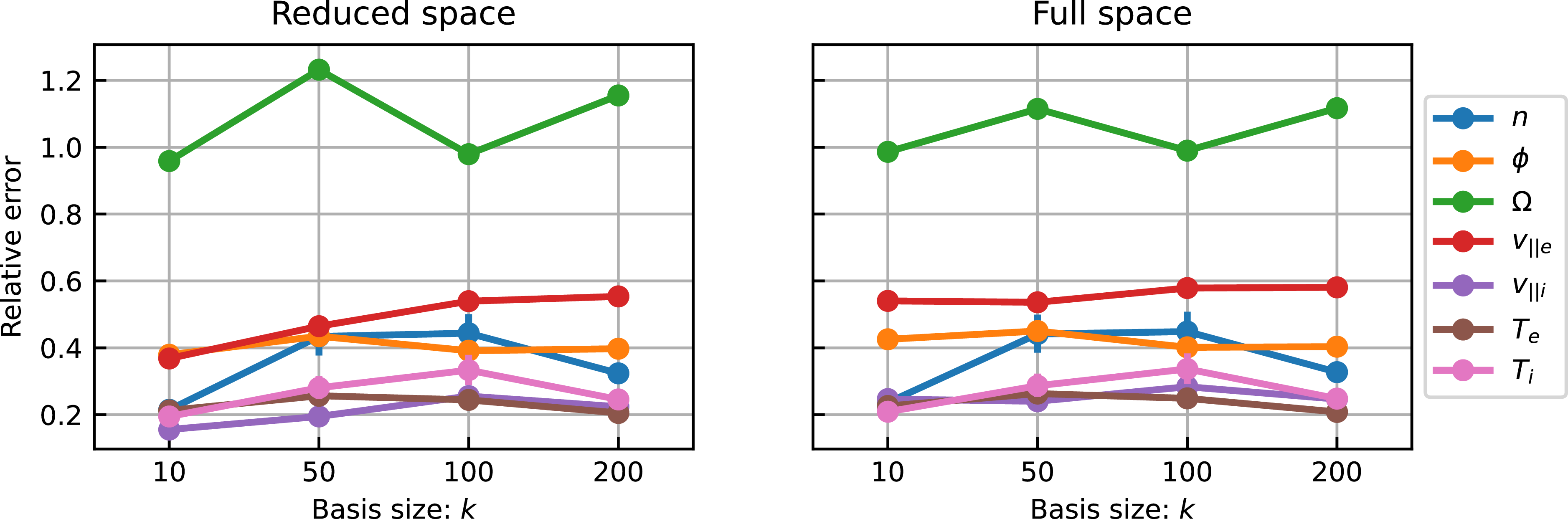


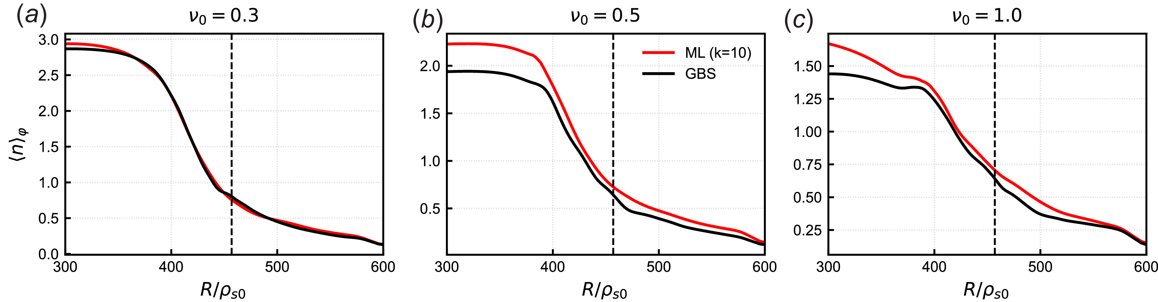


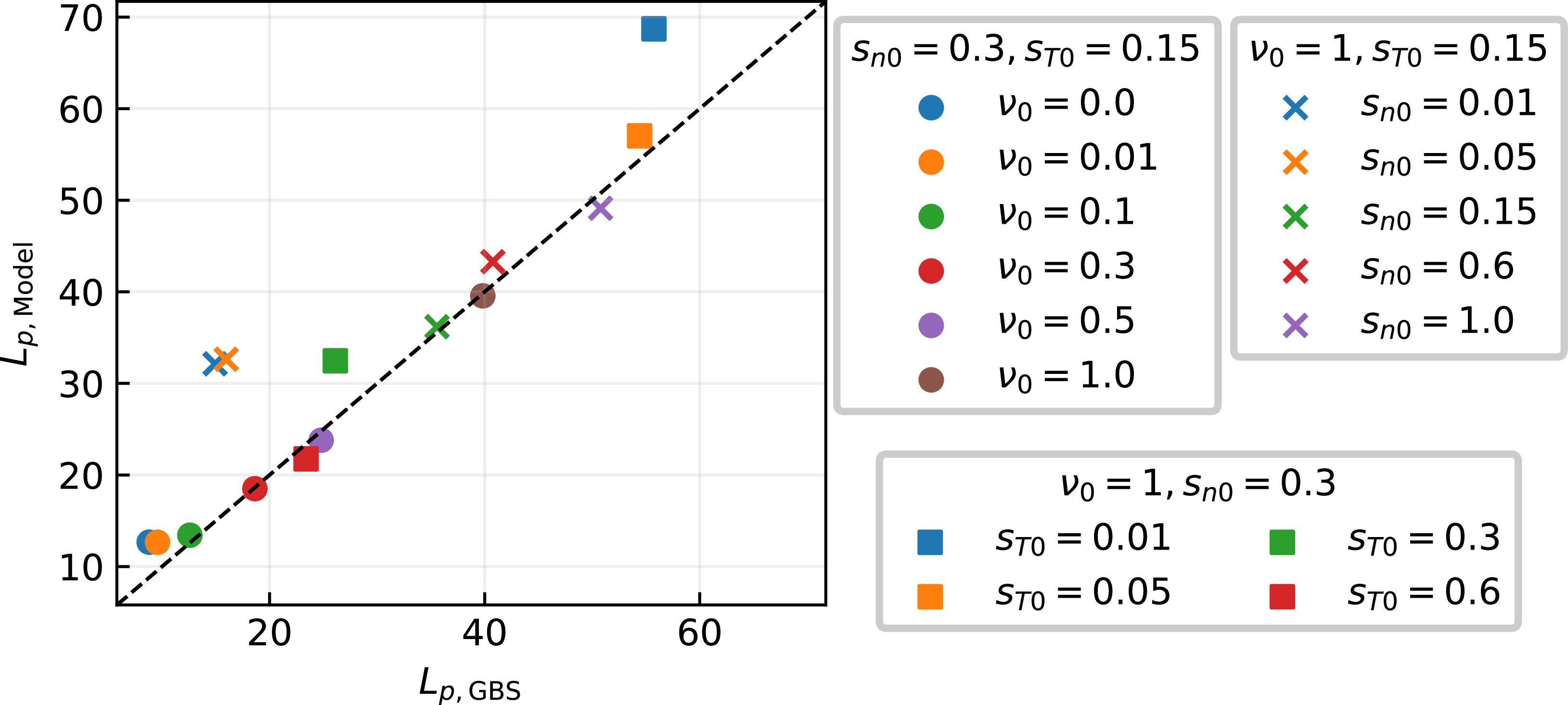


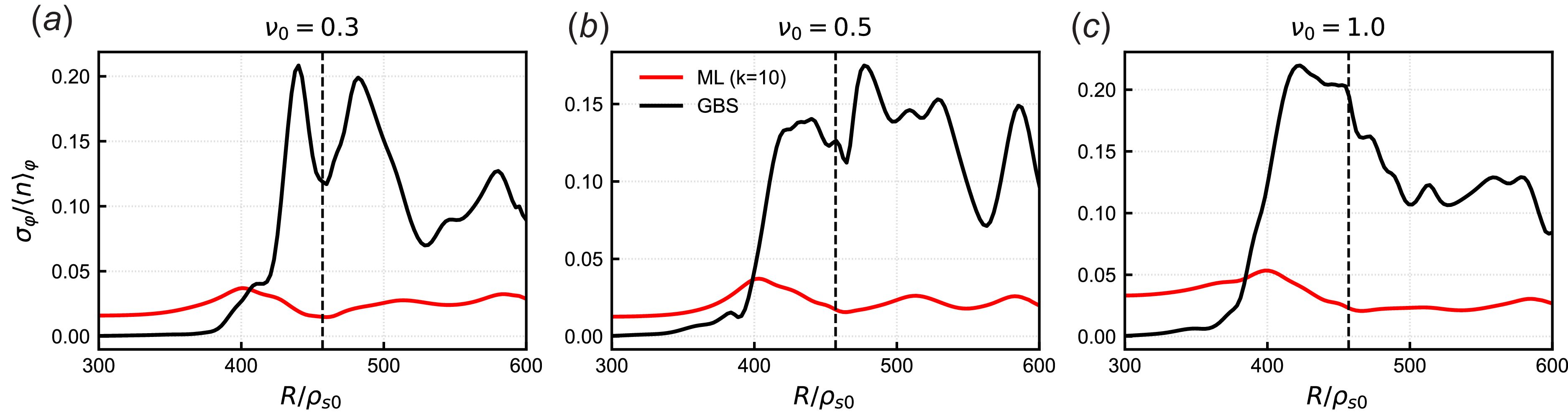


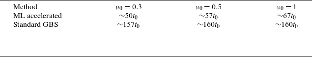


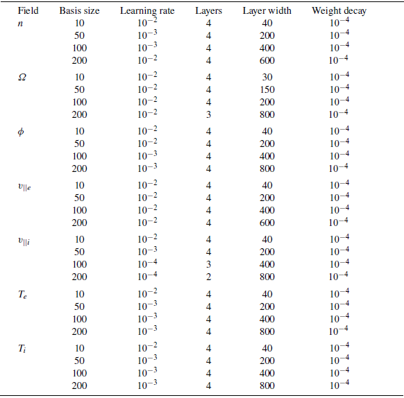


 Open access