


1. Introduction
This paper considers gradient flows in metric spaces, following the seminal work by [Reference Ambrosio, Gigli and Savaré2]. There, the authors introduce the concept of
 $p$
-curves of maximal slope, with origins dating back to [Reference De Giorgi, Marino and Tosques31]. This concept is further generalized in [Reference Rossi, Mielke and Savaré87]. As for our main contribution, we study the less-known limit case
$p$
-curves of maximal slope, with origins dating back to [Reference De Giorgi, Marino and Tosques31]. This concept is further generalized in [Reference Rossi, Mielke and Savaré87]. As for our main contribution, we study the less-known limit case
 $p=\infty$
and adapt current theory to this setting. The main incentive for our work is the adversarial attack problem as introduced in [Reference Goodfellow, Shlens and Szegedy46, Reference Szegedy, Zaremba and Sutskever101]. Here one considers a classification task, where a classifier
$p=\infty$
and adapt current theory to this setting. The main incentive for our work is the adversarial attack problem as introduced in [Reference Goodfellow, Shlens and Szegedy46, Reference Szegedy, Zaremba and Sutskever101]. Here one considers a classification task, where a classifier
 $h\;:\;\mathcal{X}\to \mathcal{Y}$
– typically parametrized as a neural network – is given an input
$h\;:\;\mathcal{X}\to \mathcal{Y}$
– typically parametrized as a neural network – is given an input
 ${x}\in \mathcal{X}$
, which it correctly classifies as
${x}\in \mathcal{X}$
, which it correctly classifies as
 $y\in \mathcal{Y}$
, where
$y\in \mathcal{Y}$
, where
 $\mathcal{Y}$
is assumed to be a subset of a finite dimensional vector space. The goal is to obtain a perturbed input
$\mathcal{Y}$
is assumed to be a subset of a finite dimensional vector space. The goal is to obtain a perturbed input
 $\tilde {{x}}\in \mathcal{X}$
, the adversarial example, which is misclassified, while its difference to
$\tilde {{x}}\in \mathcal{X}$
, the adversarial example, which is misclassified, while its difference to
 $x$
is “imperceptible”. In practice, the latter condition is enforced by requiring that
$x$
is “imperceptible”. In practice, the latter condition is enforced by requiring that
 $\tilde {{x}}$
has at most distance
$\tilde {{x}}$
has at most distance
 $\varepsilon$
to
$\varepsilon$
to
 $x$
in an
$x$
in an
 $\ell ^p$
distance, where
$\ell ^p$
distance, where
 $\varepsilon \gt 0$
is called the adversarial budget. Given some loss function
$\varepsilon \gt 0$
is called the adversarial budget. Given some loss function
 $\ell \;:\;\mathcal{Y}\times \mathcal{Y}\to {\mathbb{R}}$
, one then formulates the adversarial attack problem [Reference Goodfellow, Shlens and Szegedy46, Reference Szegedy, Zaremba and Sutskever101],
$\ell \;:\;\mathcal{Y}\times \mathcal{Y}\to {\mathbb{R}}$
, one then formulates the adversarial attack problem [Reference Goodfellow, Shlens and Szegedy46, Reference Szegedy, Zaremba and Sutskever101],
 \begin{align} \sup _{\tilde {{x}} \in \overline {B_\varepsilon }({x})} \ell (h(\tilde {{x}}),y). \end{align}
The above problem is also called an untargeted attack, since we are solely interested in the misclassification. This is opposed to targeted attacks, where one prescribes
 $y_{\text{target}}\in \mathcal{Y}$
and wants to obtain an adversarial example, s.t.
$y_{\text{target}}\in \mathcal{Y}$
and wants to obtain an adversarial example, s.t.
 $h(\tilde {{x}}) = y_{\text{target}}$
. This basically amounts to changing the loss function in (AdvAtt), namely to
$h(\tilde {{x}}) = y_{\text{target}}$
. This basically amounts to changing the loss function in (AdvAtt), namely to
 $-\ell (\cdot ,y_{\text{target}})$
, without changing the inherent structure of the problem, which is why we do not consider it separately in the following. Methods for generating adversarial examples include first-order attacks [Reference Brendel, Rauber, Kümmerer, Ustyuzhaninov and Bethge12, Reference Moosavi-Dezfooli, Fawzi and Frossard71, Reference Pintor, Roli, Brendel and Biggio80], momentum-variants [Reference Dong, Liao, Pang, Su, Zhu and Hu35], second-order attacks [Reference Jang, Wu and Jha55] or even zero-order attacks, not employing the gradient of the classifier [Reference Brendel, Rauber and Bethge11, Reference Ilyas, Engstrom, Athalye and Lin53]. Especially for classifiers induced by neural networks, it was noticed in [Reference Szegedy, Zaremba and Sutskever101] that approximate maximizers of (AdvAtt) completely corrupt the classification performance, even for a very small budget
$-\ell (\cdot ,y_{\text{target}})$
, without changing the inherent structure of the problem, which is why we do not consider it separately in the following. Methods for generating adversarial examples include first-order attacks [Reference Brendel, Rauber, Kümmerer, Ustyuzhaninov and Bethge12, Reference Moosavi-Dezfooli, Fawzi and Frossard71, Reference Pintor, Roli, Brendel and Biggio80], momentum-variants [Reference Dong, Liao, Pang, Su, Zhu and Hu35], second-order attacks [Reference Jang, Wu and Jha55] or even zero-order attacks, not employing the gradient of the classifier [Reference Brendel, Rauber and Bethge11, Reference Ilyas, Engstrom, Athalye and Lin53]. Especially for classifiers induced by neural networks, it was noticed in [Reference Szegedy, Zaremba and Sutskever101] that approximate maximizers of (AdvAtt) completely corrupt the classification performance, even for a very small budget
 $\varepsilon$
. This observation created severe concerns about the robustness and reliability of neural networks (see e.g. [Reference Kurakin, Goodfellow and Bengio59]) and has sparked a general interest in both the adversarial attack and the defence problem. The connection between the attack and defence task was already introduced in [Reference Goodfellow, Shlens and Szegedy46], where the authors propose adversarial training (similarly derived in [Reference Kurakin, Goodfellow and Bengio58, Reference Madry, Makelov, Schmidt, Tsipras and Vladu64]). Here, the standard empirical risk minimization is modified to
$\varepsilon$
. This observation created severe concerns about the robustness and reliability of neural networks (see e.g. [Reference Kurakin, Goodfellow and Bengio59]) and has sparked a general interest in both the adversarial attack and the defence problem. The connection between the attack and defence task was already introduced in [Reference Goodfellow, Shlens and Szegedy46], where the authors propose adversarial training (similarly derived in [Reference Kurakin, Goodfellow and Bengio58, Reference Madry, Makelov, Schmidt, Tsipras and Vladu64]). Here, the standard empirical risk minimization is modified to
 \begin{align} \inf _{h\in \mathcal{H}} \sum _{({x},y)\in \mathcal{T}} \sup _{\tilde {{x}}\in \overline {B_\varepsilon }({x})} \ell (h(\tilde {{x}}), y) \end{align}
for a training set
 $\mathcal{T}\subset \mathcal{X}\times \mathcal{Y}$
and a hypothesis class
$\mathcal{T}\subset \mathcal{X}\times \mathcal{Y}$
and a hypothesis class
 $\mathcal{H}\subset \{h|h\,:\,\mathcal{X}\to \mathcal{Y}\}$
. Since this requires solving (AdvAtt) for every data point
$\mathcal{H}\subset \{h|h\,:\,\mathcal{X}\to \mathcal{Y}\}$
. Since this requires solving (AdvAtt) for every data point
 $x$
, the authors then propose an efficient one-step method, called fast gradient sign method (FGSM),
$x$
, the authors then propose an efficient one-step method, called fast gradient sign method (FGSM),
 \begin{align} x_{\mathrm {FGS}}={x}+\varepsilon \, \operatorname {sign}(\nabla _{x} \ell (h({x}),y)). \end{align}
The motivation, as provided in [Reference Goodfellow, Shlens and Szegedy46], was to consider a linear model
 ${x}\mapsto \langle w, {x}\rangle$
, with weights
${x}\mapsto \langle w, {x}\rangle$
, with weights
 $w$
. The maximum over the input
$w$
. The maximum over the input
 $x$
constrained to the budget ball
$x$
constrained to the budget ball
 $\overline {B^\infty _\varepsilon }(x)$
is then attained in a corner of the hypercube, which validates the use of the sign. From a practical perspective, also for more complicated models, the sign operation ensures that
$\overline {B^\infty _\varepsilon }(x)$
is then attained in a corner of the hypercube, which validates the use of the sign. From a practical perspective, also for more complicated models, the sign operation ensures that
 $x_{\mathrm {FGS}} \in \partial B_\varepsilon ^\infty ({x})$
, i.e.,
$x_{\mathrm {FGS}} \in \partial B_\varepsilon ^\infty ({x})$
, i.e.,
 $x_{\mathrm {FGS}}$
uses all the given budget in the
$x_{\mathrm {FGS}}$
uses all the given budget in the
 $\ell ^\infty$
distance after just one update step. This adversarial training setup was similarly employed in [Reference Madry, Makelov, Schmidt, Tsipras and Vladu64, Reference Roth, Kilcher and Hofmann88, Reference Shafahi, Najibi and Ghiasi94, Reference Wong, Rice and Kolter105] and analyzed as regularization of the empirical risk in [Reference Bungert, Trillos and Murray18, Reference Bungert, Laux and Stinson20]. For other strategies to obtain robust classifiers, we refer, e.g., to [Reference Bungert, Bungert, Roith, Schwinn and Tenbrinck21, Reference Gouk, Frank, Pfahringer and Cree47, Reference Krishnan, Makdah, AlRahman and Pasqualetti57, Reference Pauli, Koch, Berberich, Kohler and Allgöwer77]. In situations where only the attack problem is of interest, multistep methods are feasible, which led to the iterative FGS method [Reference Kurakin, Goodfellow and Bengio58, Reference Kurakin, Goodfellow and Bengio59]
$\ell ^\infty$
distance after just one update step. This adversarial training setup was similarly employed in [Reference Madry, Makelov, Schmidt, Tsipras and Vladu64, Reference Roth, Kilcher and Hofmann88, Reference Shafahi, Najibi and Ghiasi94, Reference Wong, Rice and Kolter105] and analyzed as regularization of the empirical risk in [Reference Bungert, Trillos and Murray18, Reference Bungert, Laux and Stinson20]. For other strategies to obtain robust classifiers, we refer, e.g., to [Reference Bungert, Bungert, Roith, Schwinn and Tenbrinck21, Reference Gouk, Frank, Pfahringer and Cree47, Reference Krishnan, Makdah, AlRahman and Pasqualetti57, Reference Pauli, Koch, Berberich, Kohler and Allgöwer77]. In situations where only the attack problem is of interest, multistep methods are feasible, which led to the iterative FGS method [Reference Kurakin, Goodfellow and Bengio58, Reference Kurakin, Goodfellow and Bengio59]
 \begin{align} x_{\mathrm {IFGS}}^{k+1}=\Pi _{\overline {B^p_\varepsilon }({x})}(x_{\mathrm {IFGS}}^k+\tau \, \operatorname {sign}(\nabla _{x} \ell (h(x_{\mathrm {IFGS}}^k),y)) ), \end{align}
where
 $\tau \gt 0$
now defines a step size and
$\tau \gt 0$
now defines a step size and
 $\Pi _{\overline {B^p_\varepsilon }(x)}$
denotes the orthogonal projection to the
$\Pi _{\overline {B^p_\varepsilon }(x)}$
denotes the orthogonal projection to the
 $\varepsilon$
-ball in the
$\varepsilon$
-ball in the
 $\ell ^p$
-norm around the original image. Originally, the case
$\ell ^p$
-norm around the original image. Originally, the case
 $p=\infty$
was employed, where the projection is then a simple clipping operation. Other choices of
$p=\infty$
was employed, where the projection is then a simple clipping operation. Other choices of
 $p$
are usually limited to
$p$
are usually limited to
 $\{0,1,2\}$
, which is also due to the computational effort of computing the projection (see [Reference Pintor, Roli, Brendel and Biggio80] for
$\{0,1,2\}$
, which is also due to the computational effort of computing the projection (see [Reference Pintor, Roli, Brendel and Biggio80] for
 $p=0$
and [Reference Duchi, Shalev-Shwartz, Singer and Chandra36] for
$p=0$
and [Reference Duchi, Shalev-Shwartz, Singer and Chandra36] for
 $p=1$
). Signed gradient descent can also be interpreted as a form of normalized gradient descent in the
$p=1$
). Signed gradient descent can also be interpreted as a form of normalized gradient descent in the
 $\ell ^\infty$
topology as in [Reference Cortés27], where our framework allows considering a general
$\ell ^\infty$
topology as in [Reference Cortés27], where our framework allows considering a general
 $\ell ^q$
norm. Apart from the adversarial setting, signed gradient descent, without the projection step, is an established optimization algorithm itself, see e.g., [Reference Mohammadi and Janaideh70, Reference Zhang, Hui, Moulay and Coirault106] for other applications. The idea of using signed gradients can also be found in the RPROP algorithm [Reference Riedmiller and Braun83]. The convergence to minimizers of signed gradient descent and its variants was analyzed in [Reference Balles, Pedregosa and Roux5, Reference Chzhen and Schechtman26, Reference Li, Lin, Li, Hong and Chen61, Reference Moulay, Léchappé and Plestan74]. A slightly different kind of projected version, using linear constraints, was considered in [Reference Chen and Ren25], where the authors also considered a continuous time version; however, the results therein and the considered flow are not directly connected to our work here. We consider the limit
$\ell ^q$
norm. Apart from the adversarial setting, signed gradient descent, without the projection step, is an established optimization algorithm itself, see e.g., [Reference Mohammadi and Janaideh70, Reference Zhang, Hui, Moulay and Coirault106] for other applications. The idea of using signed gradients can also be found in the RPROP algorithm [Reference Riedmiller and Braun83]. The convergence to minimizers of signed gradient descent and its variants was analyzed in [Reference Balles, Pedregosa and Roux5, Reference Chzhen and Schechtman26, Reference Li, Lin, Li, Hong and Chen61, Reference Moulay, Léchappé and Plestan74]. A slightly different kind of projected version, using linear constraints, was considered in [Reference Chen and Ren25], where the authors also considered a continuous time version; however, the results therein and the considered flow are not directly connected to our work here. We consider the limit
 $\tau \to 0$
of signed gradient descent and the projected variant (IFGSM), for which we derive a gradient flow characterization. This is visualized in Figure 1. In the Euclidean setting with a differentiable energy
$\tau \to 0$
of signed gradient descent and the projected variant (IFGSM), for which we derive a gradient flow characterization. This is visualized in Figure 1. In the Euclidean setting with a differentiable energy
 $\mathcal{E}\;:\;{\mathbb{R}}^d\to {\mathbb{R}}$
and
$\mathcal{E}\;:\;{\mathbb{R}}^d\to {\mathbb{R}}$
and
 $p\in (1,\infty )$
, a differentiable curve
$p\in (1,\infty )$
, a differentiable curve
 $u\;:\;[0,T]\to {\mathbb{R}}^d$
is a
$u\;:\;[0,T]\to {\mathbb{R}}^d$
is a
 $p$
-curve of maximum slope, if it solves the
$p$
-curve of maximum slope, if it solves the
 $p$
-gradient flow equation
$p$
-gradient flow equation
 \begin{align*} \left (\left |u'\right |(t)\right )^{p-2}\, u'(t) = -\nabla \mathcal{E}(u(t)). \end{align*}
Behavior of (IFGSM) (top) and the minimizing movement scheme (MinMove) (bottom), for a binary classifier – parametrized as a neural network – on
 ${\mathbb{R}}^2$
, a budget of
${\mathbb{R}}^2$
, a budget of
 $\varepsilon =0.2$
and
$\varepsilon =0.2$
and
 $\tau \in \{0.2, 0.1, 0.02, 0.001\}$
. The white box indicates the maximal distance to the initial value, and the pink boxes indicate the step size
$\tau \in \{0.2, 0.1, 0.02, 0.001\}$
. The white box indicates the maximal distance to the initial value, and the pink boxes indicate the step size
 $\tau$
of the scheme. Details on this experiment can be found in Appendix H.
$\tau$
of the scheme. Details on this experiment can be found in Appendix H.

Here, we also refer to [Reference Bungert and Burger14, Reference Bungert, Burger, Chambolle and Novaga15] for a study of gradient-flow type equations in Hilbert spaces, for non-differentiable functionals. Following the approach in [Reference Ambrosio, Gigli and Savaré2, Reference De Giorgi, Marino and Tosques31, Reference Degiovanni, Marino and Tosques32, Reference Marino, Saccon and Tosques65], the above equation is equivalent to
 \begin{align*} \frac {\text{d}}{\text{d}t} (\mathcal{E}\circ u)\leq -\frac {1}{p}\left |u'\right |^p - \frac {1}{q}\left |\nabla \mathcal{E}(u)\right |^q, \end{align*}
where
 $1/p + 1/q = 1$
. The strength of this approach is that all derivatives in the above inequality have meaningful generalizations to the metric space setting, which we repeat in the next section. Motivated by signed gradient descent, in this paper, we draw the connection to the case
$1/p + 1/q = 1$
. The strength of this approach is that all derivatives in the above inequality have meaningful generalizations to the metric space setting, which we repeat in the next section. Motivated by signed gradient descent, in this paper, we draw the connection to the case
 $p=\infty$
. In the Euclidean setting, with a differentiable functional
$p=\infty$
. In the Euclidean setting, with a differentiable functional
 $\mathcal{E}$
, the energy dissipation inequality we derive for
$\mathcal{E}$
, the energy dissipation inequality we derive for
 $p=\infty$
reads
$p=\infty$
reads
 \begin{align*} &\left |u'\right |\leq 1,\\ &\frac {\text{d}}{\text{d}t}(\mathcal{E}\circ u)\leq -\left |\nabla \mathcal{E}(u)\right |. \end{align*}
Intuitively, a
 $\infty$
-curve of maximal slope minimizes the energy
$\infty$
-curve of maximal slope minimizes the energy
 $\mathcal{E}$
as fast as possible under the restriction that its velocity
$\mathcal{E}$
as fast as possible under the restriction that its velocity
 $\left |u'\right |$
is bounded by
$\left |u'\right |$
is bounded by
 $1$
. Like in [Reference Ambrosio, Gigli and Savaré2], our results consider general metric spaces, Banach spaces and Wasserstein spaces, which are further detailed in the following sections. Typically, curves of maximum slope can be approximated via a minimizing movement scheme, which in our case translates to
$1$
. Like in [Reference Ambrosio, Gigli and Savaré2], our results consider general metric spaces, Banach spaces and Wasserstein spaces, which are further detailed in the following sections. Typically, curves of maximum slope can be approximated via a minimizing movement scheme, which in our case translates to
 \begin{align*} x_\tau ^{k+1}\in \operatorname*{arg\,min}_{{x}\in \mathcal{X}} \{ \mathcal{E}({x})\,:\, \left \|{x} - x_\tau ^k\right \|\leq \tau \}, \end{align*}
where
 $x^0_\tau = {x}^0$
is a given initial value. A main insight, explored in section 5, is that under certain assumptions, (FGSM) and (IFGSM) fulfil this scheme, if we replace the energy by a semi-implicit version.
$x^0_\tau = {x}^0$
is a given initial value. A main insight, explored in section 5, is that under certain assumptions, (FGSM) and (IFGSM) fulfil this scheme, if we replace the energy by a semi-implicit version.
A further aspect is the characterization of adversarial attacks in the distributional setting, where the sum is replaced by an integral over the data distribution
 $\mu$
. Interchanging the integral and the supremum (see Corollary 5.7) yields the characterization of adversarial training (AdvTrain) as a distributionally robust optimization (DRO) problem,
$\mu$
. Interchanging the integral and the supremum (see Corollary 5.7) yields the characterization of adversarial training (AdvTrain) as a distributionally robust optimization (DRO) problem,
 \begin{align} \inf _{h\in \mathcal{H}}\sup _{\tilde \mu : D(\mu , \tilde \mu )\leq \varepsilon } \int \ell (h({x}), y) \,\text{d}\tilde \mu ({x},y), \end{align}
where
 $D$
denotes a distance on the space of distributions. This formulation of adversarial training was the subject of many studies in recent years, see, e.g., [Reference Bungert, Trillos and Murray18, Reference Bungert, Laux and Stinson20, Reference Bungert and Stinson22, Reference Bungert, Trillos, Jacobs, McKenzie and Wang23, Reference Zheng, Chen and Ren107]. Typically, the distance
$D$
denotes a distance on the space of distributions. This formulation of adversarial training was the subject of many studies in recent years, see, e.g., [Reference Bungert, Trillos and Murray18, Reference Bungert, Laux and Stinson20, Reference Bungert and Stinson22, Reference Bungert, Trillos, Jacobs, McKenzie and Wang23, Reference Zheng, Chen and Ren107]. Typically, the distance
 $D$
is chosen as an optimal transport distance,
$D$
is chosen as an optimal transport distance,
 \begin{align*} D(\mu ,\tilde {\mu })\;:\!=\; \inf _{\gamma \in \Gamma (\mu ,\tilde {\mu } )} \int _\gamma c((x,y),(\tilde {x},\tilde {y}))^2 d\gamma , \end{align*}
with
 $\Gamma (\mu , \tilde {\mu })$
denoting the set of all couplings and the cost
$\Gamma (\mu , \tilde {\mu })$
denoting the set of all couplings and the cost
 \begin{align} c((x,y),(\tilde {{x}},\tilde {y}))\;:\!=\; \begin{cases} \|x-\tilde {{x}}\| &\text{if } y=\tilde {y},\\ +\infty &\text{if } y\neq \tilde {y}. \end{cases} \end{align}
The goal here is then to derive a characterization of curves
 $\mu \;:\;[0,T]\to \mathcal{W}_p$
, where
$\mu \;:\;[0,T]\to \mathcal{W}_p$
, where
 $\mathcal{W}_p$
denotes the
$\mathcal{W}_p$
denotes the
 $p$
-Wasserstein space. In this regard, we mention the related work [Reference Zheng, Chen and Ren107], where the authors proposed to solve the inner optimization problem
$p$
-Wasserstein space. In this regard, we mention the related work [Reference Zheng, Chen and Ren107], where the authors proposed to solve the inner optimization problem
 \begin{align*} \sup _{\tilde \mu : D(\mu , \tilde \mu )\leq \varepsilon } \int \ell (h({x}), y) \,\text{d}\tilde \mu ({x},y) \end{align*}
by disintegrating the data distribution
 $\text{d}\mu (x,y)=\text{d}\mu _y(x)\text{d}\nu (y)$
(see Appendix E), and calculating for
$\text{d}\mu (x,y)=\text{d}\mu _y(x)\text{d}\nu (y)$
(see Appendix E), and calculating for
 $\nu$
-a.e.
$\nu$
-a.e.
 $y\in \mathcal{Y}$
the corresponding
$y\in \mathcal{Y}$
the corresponding
 $2$
-gradient flow in
$2$
-gradient flow in
 $\mathcal{W}_2$
with initial condition
$\mathcal{W}_2$
with initial condition
 $\mu _y^0$
. As shown in [Reference Ambrosio, Gigli and Savaré2], solving this gradient flow is equivalent to solving the partial differential equation
$\mu _y^0$
. As shown in [Reference Ambrosio, Gigli and Savaré2], solving this gradient flow is equivalent to solving the partial differential equation
 \begin{equation} \begin{aligned} \partial _t (\mu _y)_t&=\nabla \cdot ((\mu _y)_t \nabla _x \ell (h({x}), y)) \quad \text{on } (0,T)\\ (\mu _y)_0&=\mu _y^0, \end{aligned} \end{equation}
which is to be understood in the distributional sense. The authors in [Reference Zheng, Chen and Ren107] then approximate a maximizer by
 $\text{d}\tilde {\mu }(x,y)\approx \text{d}(\mu _y)_T (x)\text{d}\nu (y)$
, where
$\text{d}\tilde {\mu }(x,y)\approx \text{d}(\mu _y)_T (x)\text{d}\nu (y)$
, where
 $T$
has to be chosen small enough such that the approximation is still within the
$T$
has to be chosen small enough such that the approximation is still within the
 $\varepsilon$
ball around
$\varepsilon$
ball around
 $\mu$
.
$\mu$
.
In the following, we first provide the necessary notions for gradient flows in metric spaces and then proceed to discuss the main contributions and the outline of this paper.
1.1. Setup
We give a brief recap on classical notation and preliminaries on evolution in metric spaces. More details can be found in [Reference Ambrosio, Gigli and Savaré2, Reference Mielke, Rossi and Savaré68]. In the following, we denote by
 $(\mathcal{S},d)$
a complete metric space, while
$(\mathcal{S},d)$
a complete metric space, while
 $\mathcal{X}$
denotes a Banach space. We consider a proper functional
$\mathcal{X}$
denotes a Banach space. We consider a proper functional
 $\mathcal{E}\;:\; \mathcal{S}\rightarrow ({-}\infty ,+\infty ]$
, i.e., the effective domain
$\mathcal{E}\;:\; \mathcal{S}\rightarrow ({-}\infty ,+\infty ]$
, i.e., the effective domain
 $\operatorname {dom}(\mathcal{E}) \;:\!=\; \{ {x}\in \mathcal{S}\,:\, \mathcal{E}({x}) \lt \infty \}$
is assumed to be nonempty. Throughout this paper, we denote by
$\operatorname {dom}(\mathcal{E}) \;:\!=\; \{ {x}\in \mathcal{S}\,:\, \mathcal{E}({x}) \lt \infty \}$
is assumed to be nonempty. Throughout this paper, we denote by
 \begin{align*} B_\tau ({x}) \;:\!=\; \{\tilde {{x}}\in \mathcal{S}\,:\, d({x}, \tilde {{x}}) \lt \tau \}, \qquad \overline {B_\tau }({x}) \;:\!=\; \{\tilde {{x}}\in \mathcal{S}\;:\; d({x}, \tilde {{x}}) \leq \tau \} \end{align*}
the ball and its closed variant, induced by the given metric
 $d$
, where we employ the abbreviation
$d$
, where we employ the abbreviation
 $B_\tau (0) = B_\tau$
. In the finite-dimensional case, we write
$B_\tau (0) = B_\tau$
. In the finite-dimensional case, we write
 $B^p_\tau$
to denote the ball induced by the
$B^p_\tau$
to denote the ball induced by the
 $\ell ^p$
norm on
$\ell ^p$
norm on
 ${\mathbb{R}}^d$
. Note that there is a notation conflict with
${\mathbb{R}}^d$
. Note that there is a notation conflict with
 $d$
denoting both the distance and the dimension of the finite-dimensional space
$d$
denoting both the distance and the dimension of the finite-dimensional space
 ${\mathbb{R}}^d$
. However, the concrete meaning is always clear from the context.
${\mathbb{R}}^d$
. However, the concrete meaning is always clear from the context.
Metric derivative. We consider curves
 $u\;:\;[0,T]\rightarrow \mathcal{S}$
with
$u\;:\;[0,T]\rightarrow \mathcal{S}$
with
 $T\gt 0$
for which we want to have a notion of velocity. For this purpose, we need a generalization of the absolute value of the derivatives, which is provided by the metric derivative as introduced by [Reference Ambrosio1]. Here, one usually considers
$T\gt 0$
for which we want to have a notion of velocity. For this purpose, we need a generalization of the absolute value of the derivatives, which is provided by the metric derivative as introduced by [Reference Ambrosio1]. Here, one usually considers
 $p$
-absolutely continuous curves [Reference Ambrosio, Gigli and Savaré2], i.e., for
$p$
-absolutely continuous curves [Reference Ambrosio, Gigli and Savaré2], i.e., for
 $p\in [1,\infty ]$
, there exists
$p\in [1,\infty ]$
, there exists
 $m\in L^p(0,T)$
such that
$m\in L^p(0,T)$
such that
 \begin{align} d(u(t), u(s)) \leq \int _s^t m(r)\, \text{d}r \end{align}
for all
 $0\leq s\lt t \leq T$
. The set of all
$0\leq s\lt t \leq T$
. The set of all
 $p$
-absolutely continuous curves is denoted by
$p$
-absolutely continuous curves is denoted by
 $AC^p(0,T; \mathcal{S})$
. We are especially interested in the case
$AC^p(0,T; \mathcal{S})$
. We are especially interested in the case
 $p=\infty$
, where the condition in Equation (1.3) is equivalent to the Lipschitzness of the curve, i.e., the existence of a constant
$p=\infty$
, where the condition in Equation (1.3) is equivalent to the Lipschitzness of the curve, i.e., the existence of a constant
 $L\geq 0$
such that
$L\geq 0$
such that
 \begin{align*} d(u(t), u(s)) \leq L\ (t-s) \end{align*}
for all
 $0\leq s\lt t \leq T$
. For the special case
$0\leq s\lt t \leq T$
. For the special case
 $p=\infty$
, we have the following result as a special case of [Reference Ambrosio, Gigli and Savaré2, Theorem 1.1.2].
$p=\infty$
, we have the following result as a special case of [Reference Ambrosio, Gigli and Savaré2, Theorem 1.1.2].
Lemma 1.1 (Metric derivative).Let
 $u\;:\;[0,T]\rightarrow \mathcal{S}$
be a Lipschitz curve with Lipschitz constant
$u\;:\;[0,T]\rightarrow \mathcal{S}$
be a Lipschitz curve with Lipschitz constant
 $L$
, then the limit
$L$
, then the limit
 \begin{align*} |u'|(t)\;:\!=\;\lim _{s\rightarrow t}\frac {d(u(s),u(t))}{|s-t|} \end{align*}
exists for a.e.
 $t\in [0,T]$
and is referred to as the metric derivative. Moreover, the function
$t\in [0,T]$
and is referred to as the metric derivative. Moreover, the function
 $t\mapsto |u'|(t)$
belongs to
$t\mapsto |u'|(t)$
belongs to
 $L^\infty (0,T)$
with
$L^\infty (0,T)$
with
 $\||u'|\|_{L^\infty (0,T)}\leq L$
, and
$\||u'|\|_{L^\infty (0,T)}\leq L$
, and
 \begin{align*} d(u(s),u(t))\leq \int _s^t |u'|(r) \, \text{d}r \quad \ \text{for all } 0\leq s\leq t \leq T. \end{align*}
Remark 1.2. The metric derivative
 $|u'|$
is actually minimal in the sense that for every
$|u'|$
is actually minimal in the sense that for every
 $m$
satisfying (1.3),
$m$
satisfying (1.3),
 \begin{equation*} |u'|(t)\leq m(t) \quad \text{for a.e. }t\in (0,T).\end{equation*}
Remark 1.3. If
 $\mathcal{S}=\mathcal{X}$
is a Banach space and satisfies the Radon–Nikodým property (c.f. [Reference Ryan89, p. 106]), e.g., if it is reflexive, then
$\mathcal{S}=\mathcal{X}$
is a Banach space and satisfies the Radon–Nikodým property (c.f. [Reference Ryan89, p. 106]), e.g., if it is reflexive, then
 $u\in AC^p(0,T;\;\mathcal{X})$
if and only if
$u\in AC^p(0,T;\;\mathcal{X})$
if and only if
-
•
 $u$
is differentiable a.e. on
$(0,T)$
$u$
is differentiable a.e. on
$(0,T)$
-
•
$u'(t)\in L^p(0,T;\;\mathcal{X})$
-
•
$u(t)-u(s)=\int _s^t u'(t) \,\text{d}r$
for
$0\leq s\leq t\leq T$
.


Upper gradients We consider upper gradients as a generalization of the absolute value of the gradient in the metric setting. Namely, we employ the following definitions from [Reference Ambrosio, Gigli and Savaré2, Definition 1.2.1] and [Reference Ambrosio, Gigli and Savaré2, Definition 1.2.2].
Definition 1.4.
A function
 $g\;:\;\mathcal{S}\to [0, +\infty ]$
is called a strong upper gradient for
$g\;:\;\mathcal{S}\to [0, +\infty ]$
is called a strong upper gradient for
 $\mathcal{E}$
if, for every absolutely continuous curve
$\mathcal{E}$
if, for every absolutely continuous curve
 $u\;:\;[0,T]\to \mathcal{S}$
, the function
$u\;:\;[0,T]\to \mathcal{S}$
, the function
 $g\circ u$
is Borel and
$g\circ u$
is Borel and
 \begin{align} |\mathcal{E}(u(t)) -\mathcal{E}(u(s))|\leq \int _s^t g(u(r)) |u'|(r) \, \text{d}r \quad \forall \ 0\leq s\leq t\leq T \end{align}
If
 $(g\circ u)\, |u'| \in L^1(0,T)$
, then
$(g\circ u)\, |u'| \in L^1(0,T)$
, then
 $\mathcal{E}\circ u$
is absolutely continuous and
$\mathcal{E}\circ u$
is absolutely continuous and
 \begin{align} |(\mathcal{E}\circ u)'(t)|\leq g(u(t))|u'|(t) \quad \text{for a.e. } t\in (0,T). \end{align}
Definition 1.5.
A function
 $g\;:\;\mathcal{S}\to [0, +\infty ]$
is called a weak upper gradient for
$g\;:\;\mathcal{S}\to [0, +\infty ]$
is called a weak upper gradient for
 $\mathcal{E}$
, if for every absolutely continuous curve
$\mathcal{E}$
, if for every absolutely continuous curve
 $u\;:\;[0,T]\to \mathcal{S}$
that fulfils
$u\;:\;[0,T]\to \mathcal{S}$
that fulfils
-
(i)
$(g\circ u)\ \left |u^\prime \right |\in L^1(0,T)$
, -
(ii)
$\mathcal{E} \circ u$
is a.e. in
$(0,T)$
equal to a function
$\psi \;:\; (0,T)\to {\mathbb{R}}$
with bounded variation,


it follows that
 \begin{align*} \left |\psi ^\prime \right | \leq (g\circ u)\ \left |u^\prime \right | \text{ a.e. in } (0,T). \end{align*}
Remark 1.6. We note that for a function
 $\psi$
with bounded variation, i.e.,
$\psi$
with bounded variation, i.e.,
 \begin{align*} \sup \left \{ \sum _{i=0}^{N-1} \left |\psi (t_{i+1}) - \psi (t_i)\right |\,:\, 0=t_0\lt \ldots \lt t_N=T \right \} \lt \infty , \end{align*}
we have that the derivative
 $\psi ^\prime$
exists a.e. in the interval
$\psi ^\prime$
exists a.e. in the interval
 $(0,T)$
, see [Reference Saks90, Theorem 9.6, Chapter IV].
$(0,T)$
, see [Reference Saks90, Theorem 9.6, Chapter IV].
Remark 1.7. Admissible curves
 $u$
in the above definition fulfil that
$u$
in the above definition fulfil that
 $u^{-1}(\mathcal{S}\setminus \operatorname {dom}(\mathcal{E}))$
is a null set, because of (ii). Therefore, the behaviour of
$u^{-1}(\mathcal{S}\setminus \operatorname {dom}(\mathcal{E}))$
is a null set, because of (ii). Therefore, the behaviour of
 $g$
outside of
$g$
outside of
 $\operatorname {dom}(\mathcal{E})$
is negligible.
$\operatorname {dom}(\mathcal{E})$
is negligible.
Metric slope We now consider the metric slope, as defined in [Reference De Giorgi, Marino and Tosques31], as a special realization of a weak upper gradient. Intuitively, the slope gives the value of the maximal descent at a point
 $u$
at an infinitesimal small distance.
$u$
at an infinitesimal small distance.
Definition 1.8.
For a proper functional
 $\mathcal{E}\;:\;\mathcal{S}\rightarrow ({-}\infty ,+\infty ]$
, the local slope of
$\mathcal{E}\;:\;\mathcal{S}\rightarrow ({-}\infty ,+\infty ]$
, the local slope of
 $\mathcal{E}$
at
$\mathcal{E}$
at
 ${x}\in \operatorname {dom}(\mathcal{E})$
is defined as
${x}\in \operatorname {dom}(\mathcal{E})$
is defined as
 \begin{align*} |\partial \mathcal{E}|({x}) \;:\!=\; \limsup _{z\rightarrow {x}} \frac {(\mathcal{E}({x})-\mathcal{E}(z))^+}{d({x},z)}. \end{align*}
The definition of the slope does, in fact, yield an upper gradient, which is provided by the following statement from [Reference Ambrosio, Gigli and Savaré2].
Theorem 1.9 [Reference Ambrosio, Gigli and Savaré2, Theorem 1.2.5]. Let
 $\mathcal{E}$
be a proper functional, then the function
$\mathcal{E}$
be a proper functional, then the function
 $\left |\partial \mathcal{E}\right |$
is a weak upper gradient.
$\left |\partial \mathcal{E}\right |$
is a weak upper gradient.
Curves of maximal slope Curves of maximal slope were introduced in [Reference De Giorgi, Marino and Tosques31] and are a possible generalization of a gradient evolution in metric spaces. They are usually formulated for the case
 $p\in (1,\infty )$
as follows, see, e.g., [Reference Ambrosio, Gigli and Savaré2].
$p\in (1,\infty )$
as follows, see, e.g., [Reference Ambrosio, Gigli and Savaré2].
Definition 1.10 (
 $p$
-Curves of maximal slope). For
$p$
-Curves of maximal slope). For
 $p\in (1,\infty )$
, we say that an absolutely continuous curve
$p\in (1,\infty )$
, we say that an absolutely continuous curve
 $u\;:\;[0,T]\to \mathcal{S}$
is a
$u\;:\;[0,T]\to \mathcal{S}$
is a
 $p$
-curve of maximal slope, for the functional
$p$
-curve of maximal slope, for the functional
 $\mathcal{E}$
with respect to an upper gradient
$\mathcal{E}$
with respect to an upper gradient
 $g$
, if
$g$
, if
 $\mathcal{E}\circ u$
is a.e. equal to a non-increasing map
$\mathcal{E}\circ u$
is a.e. equal to a non-increasing map
 $\psi$
and
$\psi$
and
 \begin{align} \psi ^\prime (t)\leq -\frac {1}{p} \left |u^\prime \right |^p(t) -\frac {1}{q} g^q(u(t)) \end{align}
for almost every
 $t\in (0,T)$
and
$t\in (0,T)$
and
 $1=\frac {1}{p}+\frac {1}{q}$
.
$1=\frac {1}{p}+\frac {1}{q}$
.
For
 $p\in (1,\infty )$
, the existence of such curves is provided, see for example [Reference Ambrosio, Gigli and Savaré2].
$p\in (1,\infty )$
, the existence of such curves is provided, see for example [Reference Ambrosio, Gigli and Savaré2].
1.2. Main results
Here, we summarize the main contributions of this paper. The most important one is the development and application of a gradient flow framework that allows for a theoretical study of adversarial attacks. Concerning the theory of metric gradient flows, we introduce notions tailored to this application and also provide adapted proofs, as detailed below. Here, it should be noted however that many of our results in metric and Banach spaces can be obtained from the theory of doubly nonlinear equations [Reference Mielke, Rossi and Savaré69, Reference Rossi, Mielke and Savaré87]. Therefore, the main contribution from this side is to draw the connection between the previously mentioned works and the field of adversarial attacks. On top of that, the proofs that are adapted to our scenario allow for additional insights into the concrete application we consider. Beyond single adversarial examples, we also treat distributional adversaries, which we link to curves of maximal slope in the
 $\infty$
-Wasserstein space. For potential energies, we derive a (to our knowledge novel) characterization of curves of maximal slope via the superposition principle, which highlights the connection between single adversarial attacks and the distributional adversary. We give more details on the results below.
$\infty$
-Wasserstein space. For potential energies, we derive a (to our knowledge novel) characterization of curves of maximal slope via the superposition principle, which highlights the connection between single adversarial attacks and the distributional adversary. We give more details on the results below.
In section 2, we extend the notion of
 $p$
-curves of maximal slope to the case
$p$
-curves of maximal slope to the case
 $p=\infty$
, for Lipschitz curves
$p=\infty$
, for Lipschitz curves
 $u$
. As hinted in the introduction, in the limit
$u$
. As hinted in the introduction, in the limit
 $p\to \infty$
of Definition 1.10, we replace (1.6) by the following condition,
$p\to \infty$
of Definition 1.10, we replace (1.6) by the following condition,
 \begin{align*} \left |u'\right |(t)&\leq 1,\\ \quad \psi '(t)&\leq -g(u(t)). \end{align*}
Such curves are then called
 $\infty$
-curves of maximal slope. We want to highlight that similar considerations already appeared in the early works of De Giorgi, see for example, [Reference De Giorgi, Marino and Tosques31, Definition 1.2] and [Reference Giorgi43, Example 1.3]. For our concrete setup here, we dedicate section 2 to an existence proof of such curves. We note that this can also be obtained as a corollary of a more general existence result in [Reference Rossi, Mielke and Savaré87, Theorem 3.5]. Therein, the authors prove existence of curves of maximal slope fulfilling
$\infty$
-curves of maximal slope. We want to highlight that similar considerations already appeared in the early works of De Giorgi, see for example, [Reference De Giorgi, Marino and Tosques31, Definition 1.2] and [Reference Giorgi43, Example 1.3]. For our concrete setup here, we dedicate section 2 to an existence proof of such curves. We note that this can also be obtained as a corollary of a more general existence result in [Reference Rossi, Mielke and Savaré87, Theorem 3.5]. Therein, the authors prove existence of curves of maximal slope fulfilling
 \begin{align*} \psi '(t) \leq -f^*(g(u(t))) - f(\left |u'\right |(t)) \end{align*}
for a convex and lower semicontinuous function
 $f\;:\;[0,\infty )\to [0,\infty ]$
. When choosing
$f\;:\;[0,\infty )\to [0,\infty ]$
. When choosing
 $f=\chi _{[0,1]}$
, we recover our notion of
$f=\chi _{[0,1]}$
, we recover our notion of
 $\infty$
-curves of maximal slope. Although the existence proof in section 2 employs similar concepts, we choose to include it here. On the one hand, the treatment of this specific case allows for certain arguments that are not directly possible in the general case. On the other hand, this already introduces the main steps for the convergence proof in section 3, which can not directly be deduced from [Reference Rossi, Mielke and Savaré87]. The existence result in Theorem 2.11 is summarized below.
$\infty$
-curves of maximal slope. Although the existence proof in section 2 employs similar concepts, we choose to include it here. On the one hand, the treatment of this specific case allows for certain arguments that are not directly possible in the general case. On the other hand, this already introduces the main steps for the convergence proof in section 3, which can not directly be deduced from [Reference Rossi, Mielke and Savaré87]. The existence result in Theorem 2.11 is summarized below.
Existence:
Under the assumptions specified in section 2
, for every
 $\mathcal{E}\;:\;\mathcal{S}\to ({-}\infty ,+\infty ]$
and for every
$\mathcal{E}\;:\;\mathcal{S}\to ({-}\infty ,+\infty ]$
and for every
 ${x}^0 \in \operatorname {dom}(\mathcal{E})$
, there exists a 1-Lipschitz curve
${x}^0 \in \operatorname {dom}(\mathcal{E})$
, there exists a 1-Lipschitz curve
 $u\;:\;[0,T]\to \mathcal{S}$
with
$u\;:\;[0,T]\to \mathcal{S}$
with
 $u(0)={x}^0$
, which is an
$u(0)={x}^0$
, which is an
 $\infty$
-curve of maximum slope for
$\infty$
-curve of maximum slope for
 $\mathcal{E}$
with respect to its strong upper gradient
$\mathcal{E}$
with respect to its strong upper gradient
 $|\partial \mathcal{E} |$
.
$|\partial \mathcal{E} |$
.
In section 3, we consider the specific case of
 $\infty$
-curves of maximal slope in a Banach space
$\infty$
-curves of maximal slope in a Banach space
 $\mathcal{X}$
, and an energy
$\mathcal{X}$
, and an energy
 $E$
that is a
$E$
that is a
 $C^1$
perturbation of a convex function. Note that here and in the following, when the functional takes the role of a
$C^1$
perturbation of a convex function. Note that here and in the following, when the functional takes the role of a
 $C^1$
-perturbation as in section 3, we use the symbol
$C^1$
-perturbation as in section 3, we use the symbol
 $E$
instead of
$E$
instead of
 $\mathcal{E}$
. We derive an equivalent characterization of
$\mathcal{E}$
. We derive an equivalent characterization of
 $\infty$
-curves of maximal slope via a differential inclusion. We note that this differential inclusion can be obtained from [Reference Rossi, Mielke and Savaré87, Proposition 8.2], with the same choice of
$\infty$
-curves of maximal slope via a differential inclusion. We note that this differential inclusion can be obtained from [Reference Rossi, Mielke and Savaré87, Proposition 8.2], with the same choice of
 $f$
as for the existence result above. The statement in our setting can be found in Theorem 3.8 and is summarized below.
$f$
as for the existence result above. The statement in our setting can be found in Theorem 3.8 and is summarized below.
Differential inclusion:
Let
 $E: \mathcal{X} \rightarrow ({-}\infty ,+\infty ]$
satisfy (3.7) and
$E: \mathcal{X} \rightarrow ({-}\infty ,+\infty ]$
satisfy (3.7) and
 $u\;:\;[0,1] \rightarrow \mathcal{X}$
be an a.e. differentiable Lipschitz curve. Let further
$u\;:\;[0,1] \rightarrow \mathcal{X}$
be an a.e. differentiable Lipschitz curve. Let further
 $E\circ u$
be a.e. equal to a non-increasing function
$E\circ u$
be a.e. equal to a non-increasing function
 $\psi$
, then the following are equivalent:
$\psi$
, then the following are equivalent:
-
(i)
$|u'|(t)\leq 1$
and
$\psi '(t)\leq -|\partial E |(u(t))$
for a.e.
$t\in [0,1]$
, -
(ii)
$u'(t)\ \in \ \partial \|\cdot \|_*({-}\xi ) \quad \forall \xi \in \partial ^\circ E (u(t)) \not = \emptyset ,$
for a.e.
$t\in [0,1],$


where
 $\partial ^\circ E (u(t))$
denotes the elements of minimal norm of
$\partial ^\circ E (u(t))$
denotes the elements of minimal norm of
 $\partial E (u(t))$
.
$\partial E (u(t))$
.
For an energy
 $ E = E ^{\mathrm{d}}+ E ^{\mathrm{c}}$
consisting of a differentiable part
$ E = E ^{\mathrm{d}}+ E ^{\mathrm{c}}$
consisting of a differentiable part
 $ E^{\mathrm{d}}$
and a convex part
$ E^{\mathrm{d}}$
and a convex part
 $E ^{\mathrm{c}}$
, we consider the linearization in the differentiable part around a point
$E ^{\mathrm{c}}$
, we consider the linearization in the differentiable part around a point
 $z$
,
$z$
,
 \begin{align*} E ^{\mathrm{sl}}({x}; z)\;:\!=\; E ^{\mathrm{d}}(z)+\langle D E ^{\mathrm{d}}(z),{x}-z\rangle + E ^{\mathrm{c}}({x}). \end{align*}
This then leads us to the semi-implicit minimizing movement scheme in Definition 3.10
 \begin{align*} x_{\mathrm {si},\tau }^{k+1}\in \operatorname*{arg\,min}\limits _{{x}\in \overline {B_\tau }(x_{\mathrm {si},\tau }^k)} E ^{\mathrm{sl}}({x};\,x_{\mathrm {si},\tau }^k), \end{align*}
which we also employ to approximate curves of maximal slope. In the case of
 $p=2$
, we refer to [Reference Fleißner40, Reference Stefanelli98] for other works that also consider approximate minimizing movement schemes. This semi-implicit scheme is useful, since in the finite dimensional adversarial setting, it allows us to choose
$p=2$
, we refer to [Reference Fleißner40, Reference Stefanelli98] for other works that also consider approximate minimizing movement schemes. This semi-implicit scheme is useful, since in the finite dimensional adversarial setting, it allows us to choose
 $-\ell (h(\cdot ),y)$
as the differentiable part, and additionally to incorporate the budget constraint via the indicator function
$-\ell (h(\cdot ),y)$
as the differentiable part, and additionally to incorporate the budget constraint via the indicator function
 $\chi _{\overline {B_\varepsilon }({x})}$
. We denote by
$\chi _{\overline {B_\varepsilon }({x})}$
. We denote by
 $\bar {x}_{\mathrm{si},\tau }$
the step function associated to the iterates
$\bar {x}_{\mathrm{si},\tau }$
the step function associated to the iterates
 $x_{\mathrm {si},\tau }^{k}$
, see Definition 3.10. We can show that up to a subsequence, this scheme also converges to an
$x_{\mathrm {si},\tau }^{k}$
, see Definition 3.10. We can show that up to a subsequence, this scheme also converges to an
 $\infty$
-curve of maximum slope in the topology
$\infty$
-curve of maximum slope in the topology
 $\sigma$
as specified in Assumption 1.a. The result can be found in Theorem 3.16, which we hint at below.
$\sigma$
as specified in Assumption 1.a. The result can be found in Theorem 3.16, which we hint at below.
Convergence to curves of maximal slope:
Under the assumptions specified in section 3
, there exists a
 $\infty$
-curve of maximal slope
$\infty$
-curve of maximal slope
 $u$
and a subsequence of
$u$
and a subsequence of
 $\tau _n=T/n$
such that
$\tau _n=T/n$
such that
 \begin{align*} \bar {x}_{\mathrm{si},\tau _n}(t) \stackrel {\sigma }{\rightharpoonup }u(t) \text{ as } n\rightarrow \infty \quad \forall t\in [0,T]. \end{align*}
In order to better understand the connection between the differential inclusion and (IFGSM), we want to highlight that
 $\infty$
-curves of maximum slope yield a general concept, which is not directly tied to signed gradient descent and the choice of the projection. The intuition behind
$\infty$
-curves of maximum slope yield a general concept, which is not directly tied to signed gradient descent and the choice of the projection. The intuition behind
 $\infty$
-curves is rather connected to employing normalized gradient descent (NGD) [Reference Cortés27]. Choosing
$\infty$
-curves is rather connected to employing normalized gradient descent (NGD) [Reference Cortés27]. Choosing
 $({\mathbb{R}}^d, \left \|\cdot \right \|_p)$
as the underlying Banach space, in section 5 we see that for
$({\mathbb{R}}^d, \left \|\cdot \right \|_p)$
as the underlying Banach space, in section 5 we see that for
 $1/p + 1/q=1$
the following iteration fulfils the semi-implicit minimizing movement scheme,
$1/p + 1/q=1$
the following iteration fulfils the semi-implicit minimizing movement scheme,
 \begin{align*} {x}^{k+1} = {x}^k + \tau \ \operatorname {sign}(\nabla _{x} E ({x}^k))\cdot \left (\frac {\left |\nabla _{x} E ({x}^k)\right |}{\left \|\nabla _{x} E ({x}^k)\right \|_q}\right )^{q-1}, \end{align*}
where the absolute value and multiplication are understood entrywise. Choosing
 $p=2$
or
$p=2$
or
 $p=\infty$
recovers the notion of NGD as in [Reference Cortés27]. Normalized gradient methods have gained significant attention outside the adversarial context. For example, in the context of saddle point evasion [Reference Hazan, Levy and Shalev-Shwartz50, Reference Levy60, Reference Murray, Swenson and Kar75], subgradient corruption [Reference Turan, Uribe, Wai and Alizadeh103], machine learning [Reference Cutkosky and Mehta28] and even variational quantum algorithms [Reference Suzuki, Yano, Raymond and Yamamoto100]. In the setting of adversarial attacks, normalization means that we want to ensure that the iterates exploit the maximum allowed budget (locally on
$p=\infty$
recovers the notion of NGD as in [Reference Cortés27]. Normalized gradient methods have gained significant attention outside the adversarial context. For example, in the context of saddle point evasion [Reference Hazan, Levy and Shalev-Shwartz50, Reference Levy60, Reference Murray, Swenson and Kar75], subgradient corruption [Reference Turan, Uribe, Wai and Alizadeh103], machine learning [Reference Cutkosky and Mehta28] and even variational quantum algorithms [Reference Suzuki, Yano, Raymond and Yamamoto100]. In the setting of adversarial attacks, normalization means that we want to ensure that the iterates exploit the maximum allowed budget (locally on
 $\overline {B_\tau }({x}^k)$
ball) in each step. This was similarly observed in [Reference Dong, Liao, Pang, Su, Zhu and Hu35]. As long as the iterates stay within the given budget
$\overline {B_\tau }({x}^k)$
ball) in each step. This was similarly observed in [Reference Dong, Liao, Pang, Su, Zhu and Hu35]. As long as the iterates stay within the given budget
 $\varepsilon$
, one can directly show that (IFGSM) is an explicit solution to the semi-implicit scheme and therefore converges to
$\varepsilon$
, one can directly show that (IFGSM) is an explicit solution to the semi-implicit scheme and therefore converges to
 $\infty$
-curves of maximum slope. In the more interesting case, where the projection has an effect, we need to ensure that minimizing on
$\infty$
-curves of maximum slope. In the more interesting case, where the projection has an effect, we need to ensure that minimizing on
 $\overline {B_\tau ^p}({x})$
and then projecting to
$\overline {B_\tau ^p}({x})$
and then projecting to
 $\overline {B_\varepsilon ^p}({x}^0)$
is equivalent to directly minimizing on
$\overline {B_\varepsilon ^p}({x}^0)$
is equivalent to directly minimizing on
 $\overline {B_\varepsilon ^p}({x}^0)\cap \overline {B_\tau ^p}({x})$
. We show this property for the case
$\overline {B_\varepsilon ^p}({x}^0)\cap \overline {B_\tau ^p}({x})$
. We show this property for the case
 $p=\infty$
in Lemma 5.4. Employing the convergence result for the semi-implicit minimizing movement scheme, then yields the convergence up to subsequences of (IFGSM), employing the
$p=\infty$
in Lemma 5.4. Employing the convergence result for the semi-implicit minimizing movement scheme, then yields the convergence up to subsequences of (IFGSM), employing the
 $\ell ^\infty$
norm. Denoting by
$\ell ^\infty$
norm. Denoting by
 $x_{\mathrm {IFGS}, \tau }^k$
the
$x_{\mathrm {IFGS}, \tau }^k$
the
 $k$
-th iterate obtained in (IFGSM) with stepsize
$k$
-th iterate obtained in (IFGSM) with stepsize
 $\tau$
, Corollary 5.3 then presents the following result.
$\tau$
, Corollary 5.3 then presents the following result.
Convergence of IFGSM:
Under the assumptions specified in section 5
, for
 $T\gt 0$
, there exists a
$T\gt 0$
, there exists a
 $\infty$
-curve of maximal slope
$\infty$
-curve of maximal slope
 $u\;:\;[0,T]\to {\mathbb{R}}^d$
, with respect to
$u\;:\;[0,T]\to {\mathbb{R}}^d$
, with respect to
 $E$
, and a subsequence of
$E$
, and a subsequence of
 $\tau _n\;:\!=\;T/n$
such that
$\tau _n\;:\!=\;T/n$
such that
 \begin{align*} \left \|x_{\mathrm {IFGS}, \tau _{n_i}}^{\lceil t/\tau _{n_i} \rceil } - u(t)\right \|\xrightarrow {i\to \infty } 0\qquad \text{ for all } t\in [0,T]. \end{align*}
In section 4, we consider potential energies
 \begin{equation*} \mathcal{E}\;:\; W_\infty (\mathcal{X})\ni \mu \mapsto \int {E}(x) \,\text{d} \mu (x),\end{equation*}
where in our context, the potential
 ${E}\;:\; \mathcal{X}\rightarrow ({-}\infty ,+\infty ]$
has the form
${E}\;:\; \mathcal{X}\rightarrow ({-}\infty ,+\infty ]$
has the form
 ${E}({x}) = -\ell (h({x}),y)$
. The basis for our main result in this section is given by [Reference Lisini63, Theorem 3.1], which is repeated as Theorem 4.7 in this paper. Namely, we characterize absolutely continuous curves
${E}({x}) = -\ell (h({x}),y)$
. The basis for our main result in this section is given by [Reference Lisini63, Theorem 3.1], which is repeated as Theorem 4.7 in this paper. Namely, we characterize absolutely continuous curves
 $\mu \in {\mathrm{AC}}^p(0,T; \mathcal{W}_p)$
by a measure
$\mu \in {\mathrm{AC}}^p(0,T; \mathcal{W}_p)$
by a measure
 $\eta$
on the space of curves
$\eta$
on the space of curves
 $u\;:\;[0,T]\to \mathcal{X}$
, which is concentrated on
$u\;:\;[0,T]\to \mathcal{X}$
, which is concentrated on
 ${\mathrm{AC}}^p(0,T;\;\mathcal{X}$
). Using this representation, in Theorem 4.18, we show that being a
${\mathrm{AC}}^p(0,T;\;\mathcal{X}$
). Using this representation, in Theorem 4.18, we show that being a
 $\infty$
-curve of maximum slope in the Wasserstein space is equivalent to the differential inclusion on the underlying Banach space, for
$\infty$
-curve of maximum slope in the Wasserstein space is equivalent to the differential inclusion on the underlying Banach space, for
 $\eta$
-a.e. curve.
$\eta$
-a.e. curve.
Characterization of curves in Wasserstein space:
Under the assumptions specified in Theorem 4.18
, for a curve
 $\mu \in {\mathrm{AC}}^\infty (0,T ; \mathcal{W} _\infty )$
with
$\mu \in {\mathrm{AC}}^\infty (0,T ; \mathcal{W} _\infty )$
with
 $\eta$
from Theorem 4.7
, the following statements are equivalent:
$\eta$
from Theorem 4.7
, the following statements are equivalent:
-
(i) The curve
$\mu$
is
$\infty$
-curve of maximal slope w.r.t. to the weak upper gradient
$\left |\partial \mathcal{E}\right |$
. -
(ii) For
$\eta$
-a.e. curve
$u\in C(0,T;\;\mathcal{X})$
it holds that
$E\circ u$
is for a.e.
$t\in (0,T)$
, equal to a non-increasing map
$\psi _u$
and
\begin{equation*} u'(t)\ \in \ \partial \|\cdot \|_*({-}\xi ) \quad \forall \xi \in \partial ^\circ {E}(u(t)) \not = \emptyset , \quad \text{for a.e. } t\in (0,T).\end{equation*}


When applying this result to adversarial training, we slightly deviate from the Wasserstein setting by choosing the extended distance in (1.1) and the associated transport distance in order to prohibit mass transport into the label direction.
Here, we want to refer to other works considering distributional adversarial attacks, e.g., [Reference Bungert, Trillos and Murray18, Reference Bungert, Trillos, Jacobs, McKenzie and Wang23, Reference Mehrabi, Javanmard, Rossi, Rao and Mai66, Reference Pydi and Jog81, Reference Pydi and Jog82, Reference Sinha, Namkoong, Volpi and Duchi96, Reference Staib and Jegelka97, Reference Zheng, Chen and Ren107]. We can adjust the arguments in section 4 to derive an analogous result for the energy
 $\mathcal{E}(\mu )\;:\!=\;\int -\ell (h(x),y) \,\text{d}\mu (x,y)$
, which we state in Theorem 5.10. Here, we only enforce the budget constraint by setting the end time of the flow to
$\mathcal{E}(\mu )\;:\!=\;\int -\ell (h(x),y) \,\text{d}\mu (x,y)$
, which we state in Theorem 5.10. Here, we only enforce the budget constraint by setting the end time of the flow to
 $T=\varepsilon$
.
$T=\varepsilon$
.
1.3. Outline
The paper is organized as follows: In section 2, we start by introducing
 $\infty$
-curves of maximal slope, as the limit case of
$\infty$
-curves of maximal slope, as the limit case of
 $p$
-curves of maximal slope. Section 2.3 then provides an existence result for those curves in a general metric setting. The underlying assumptions for its proof are stated in Section 2.1.
$p$
-curves of maximal slope. Section 2.3 then provides an existence result for those curves in a general metric setting. The underlying assumptions for its proof are stated in Section 2.1.
In section 3, we consider
 $\infty$
-curves of maximal slope when the underlying metric space is a Banach space. Section 3.1 introduces
$\infty$
-curves of maximal slope when the underlying metric space is a Banach space. Section 3.1 introduces
 $C^1$
-perturbations of convex functions as a convenient class of functionals that covers most of the energies we consider in this paper. In section 3.2, we derive equivalent characterizations of
$C^1$
-perturbations of convex functions as a convenient class of functionals that covers most of the energies we consider in this paper. In section 3.2, we derive equivalent characterizations of
 $\infty$
-curves of maximal slope via a doubly nonlinear differential inclusion. This section is concluded by investigating first-order approximation techniques of those differential inclusions in section 3.3.
$\infty$
-curves of maximal slope via a doubly nonlinear differential inclusion. This section is concluded by investigating first-order approximation techniques of those differential inclusions in section 3.3.
Section 4 is devoted to
 $\infty$
-curves of maximal slope, when the underlying space is the
$\infty$
-curves of maximal slope, when the underlying space is the
 $\infty$
-Wasserstein space. For potential energies, we give an equivalent characterization of
$\infty$
-Wasserstein space. For potential energies, we give an equivalent characterization of
 $\infty$
-curves of maximal slope via a probability measures
$\infty$
-curves of maximal slope via a probability measures
 $\eta$
on the space
$\eta$
on the space
 $C(0,T;\;\mathcal{X})$
, which is concentrated on
$C(0,T;\;\mathcal{X})$
, which is concentrated on
 $\infty$
-curves of maximal slope on the underlying Banach space
$\infty$
-curves of maximal slope on the underlying Banach space
 $\mathcal{X}$
. From
$\mathcal{X}$
. From
 $\eta$
, we can then derive a corresponding continuity equation for those curves of maximal slope.
$\eta$
, we can then derive a corresponding continuity equation for those curves of maximal slope.
In section 5, we discuss the application of differential inclusions derived in section 3 to generate adversarial examples. We show that the popular FGSM and its iterative variant (IFGSM) are simple first-order approximations of
 $\infty$
-curves of maximal slope. Insection 5.2, we rewrite adversarial training as a distributional robust optimization problem and discuss the usage of
$\infty$
-curves of maximal slope. Insection 5.2, we rewrite adversarial training as a distributional robust optimization problem and discuss the usage of
 $\infty$
-curves in the corresponding probability space to generate distributional adversaries.
$\infty$
-curves in the corresponding probability space to generate distributional adversaries.
2. Infinity flows in metric spaces
In this section, we generalize the notion of
 $p$
-curves of maximal slope to the case
$p$
-curves of maximal slope to the case
 $p=\infty$
. We consider the convex function
$p=\infty$
. We consider the convex function
 $f(x)=\frac {1}{p}|x|^p$
, which allows us to express the energy dissipation inequality (1.6) in Definition 1.10 as follows,
$f(x)=\frac {1}{p}|x|^p$
, which allows us to express the energy dissipation inequality (1.6) in Definition 1.10 as follows,
 \begin{align} \psi '(t)\leq -f(|u'|(t))-f^*(g(u(t))), \end{align}
where
 $f^*(x^*)=\frac {1}{q} |x^*|^q$
denotes the convex conjugate of
$f^*(x^*)=\frac {1}{q} |x^*|^q$
denotes the convex conjugate of
 $f$
. Considering the above inequality for arbitrary convex functions
$f$
. Considering the above inequality for arbitrary convex functions
 $f$
leads to the general framework as introduced in [Reference Rossi, Mielke and Savaré87]. For our setting, we consider the indicator function, which is obtained as the following pointwise limit,
$f$
leads to the general framework as introduced in [Reference Rossi, Mielke and Savaré87]. For our setting, we consider the indicator function, which is obtained as the following pointwise limit,
 \begin{align*} \frac {1}{p} \left |x\right |^p \xrightarrow []{p\to \infty }\chi _{[-1,1]}(x) = \begin{cases} 0 \text{ if } |x|\leq 1,\\ +\infty \text{ else}, \end{cases} \end{align*}
where
 $\chi _{[-1,1]}$
is a convex function with conjugate
$\chi _{[-1,1]}$
is a convex function with conjugate
 $\chi _{[-1,1]}^*(x^*) = x^*$
. Using
$\chi _{[-1,1]}^*(x^*) = x^*$
. Using
 $f=\chi _{[-1,1]}$
in (2.1) forces the curves of maximal slope to obey
$f=\chi _{[-1,1]}$
in (2.1) forces the curves of maximal slope to obey
 $\left |u^\prime \right |\leq 1$
almost everywhere and the energy dissipation inequality becomes
$\left |u^\prime \right |\leq 1$
almost everywhere and the energy dissipation inequality becomes
 \begin{align*} \psi '(t)\leq - (g\circ u) (t), \end{align*}
which motivates the following definition.
Definition 2.1 (
 $\infty$
-Curve of maximal slope). We say an absolutely continuous curve
$\infty$
-Curve of maximal slope). We say an absolutely continuous curve
 $u\;:\;[0,T] \rightarrow \mathcal{S}$
is an
$u\;:\;[0,T] \rightarrow \mathcal{S}$
is an
 $\infty$
-curve of maximal slope for the functional
$\infty$
-curve of maximal slope for the functional
 $\mathcal{E}$
with respect to an upper gradient
$\mathcal{E}$
with respect to an upper gradient
 $g$
, if
$g$
, if
 $\mathcal{E} \circ u$
is a.e. equal to a non-increasing map
$\mathcal{E} \circ u$
is a.e. equal to a non-increasing map
 $\psi$
and
$\psi$
and
 \begin{align} |u'|(t)&\leq 1, \nonumber \\ \quad \psi '(t)&\leq - (g\circ u)(t), \end{align}
holds for a.e.
 $t\in (0,T)$
.
$t\in (0,T)$
.
Remark 2.2. We note that the condition
 $\left |u^\prime \right |\leq 1$
a.e. implies that
$\left |u^\prime \right |\leq 1$
a.e. implies that
 $u$
is a Lipschitz curve with Lipschitz constant
$u$
is a Lipschitz curve with Lipschitz constant
 $1$
, see Lemma 1.1.
$1$
, see Lemma 1.1.
Remark 2.3. (Dissipation equality). If
 $g$
is a strong upper gradient of
$g$
is a strong upper gradient of
 $\mathcal{E}$
and
$\mathcal{E}$
and
 $\psi : [0,T] \rightarrow {\mathbb{R}}$
is finite then by Definition 1.4 and (InfFlow)
$\psi : [0,T] \rightarrow {\mathbb{R}}$
is finite then by Definition 1.4 and (InfFlow)
 \begin{equation*} | \mathcal{E}(u(t))-\mathcal{E}(u(s))| \leq \int _s^t g(u(r))|u'|(r)\,\text{d}r\leq \int _s^t g(u(r)) \,\text{d}r\leq \int _s^t -\psi '(r) \,\text{d}r\leq \psi (s)-\psi (t)\lt +\infty , \end{equation*}
where in the last inequality we use that non-increasing functions are differentiable a.e. and an upper bound on the second fundamental theorem of calculus holds [Reference Tao102, Proposition 1.6.37]. This in particular implies that
 $\mathcal{E}\circ u$
is absolutely continuous and
$\mathcal{E}\circ u$
is absolutely continuous and
 $\psi (t)=(\mathcal{E}\circ u)(t)$
for all
$\psi (t)=(\mathcal{E}\circ u)(t)$
for all
 $t\in (0,T)$
(see Lemma E.1). Furthermore, Remark 1.3 implies
$t\in (0,T)$
(see Lemma E.1). Furthermore, Remark 1.3 implies
 \begin{align*} \mathcal{E}(u(t))-\mathcal{E}(u(s))=\int _s^t (\mathcal{E}\circ u)'(r)\,\text{d}r \quad \text{for }0\leq s\leq t \leq T \end{align*}
and we can estimate
 \begin{equation*} \mathcal{E}(u(t))-\mathcal{E}(u(s))=\int _s^t (\mathcal{E}\circ u)'(r) \,\text{d}r\leq \int _s^t -d(u(r)) \,\text{d}r \quad \text{for }0\leq s\leq t \leq T \end{equation*}
and on the other hand, using (1.5), we obtain
 \begin{align*} \mathcal{E}(u(t))-\mathcal{E}(u(s))&=\int _s^t (\mathcal{E} \circ u)'(r) \,\text{d}r\geq \int _s^t -|(\mathcal{E} \circ u)'(r)| \,\text{d}r \\ &\geq \int _s^t -g(u(r)) |u'|(r) \,\text{d}r \geq \int _s^t -g(u(r)) \,\text{d}r \end{align*}
for
 $0\leq s\leq t \leq T$
. Therefore, the energy dissipation equality
$0\leq s\leq t \leq T$
. Therefore, the energy dissipation equality
 \begin{align} \mathcal{E}(u(t))-\mathcal{E}(u(s))= \int _s^t -g(u(r)) \,\text{d}r \end{align}
holds for every
 $0\leq s\leq t \leq T$
.
$0\leq s\leq t \leq T$
.
Example 1.
As an easy example, let us look at the quadratic energy
 $\mathcal{E}\;:\; {x}\mapsto \frac {1}{2} {x}^2$
on the space
$\mathcal{E}\;:\; {x}\mapsto \frac {1}{2} {x}^2$
on the space
 $(\mathcal{S}, d) = (\mathbb{R},|\cdot - \cdot |)$
. Its metric slope and thus weak upper gradient is given by
$(\mathcal{S}, d) = (\mathbb{R},|\cdot - \cdot |)$
. Its metric slope and thus weak upper gradient is given by
 $\left |\partial \mathcal{E}\right |({x}) = \left |\frac {\text{d}}{dx}\mathcal{E}\right |({x})=\left |{x}\right |$
. We choose
$\left |\partial \mathcal{E}\right |({x}) = \left |\frac {\text{d}}{dx}\mathcal{E}\right |({x})=\left |{x}\right |$
. We choose
 ${x}^0=1$
as the starting point, then the corresponding
${x}^0=1$
as the starting point, then the corresponding
 $\infty$
-curve of maximal slope is
$\infty$
-curve of maximal slope is
 \begin{equation*}u(t)=\begin{cases} 1-t &\text{if } 0\leq t\leq 1,\\ 0 &\text{if }t\gt 1 \end{cases}.\end{equation*}
We directly observe that
 $\left |u'\right |\leq 1$
and
$\left |u'\right |\leq 1$
and
 \begin{align*} \mathcal{E}(u(t)) = \begin{cases} \frac {1}{2} (1-t)^2 &\text{if } 0\leq t\leq 1,\\ 0 &\text{if }t\gt 1, \end{cases} \end{align*}
is a non-increasing map with
 \begin{align*} \frac {\text{d}}{\text{d}t} \mathcal{E}(u(t)) = \begin{cases} t-1 &\text{if } 0\leq t \lt 1,\\ 0 &\text{if }t\gt 1, \end{cases} = -\left |u(t)\right | = - \left |\partial \mathcal{E}\right |(u(t)), \end{align*}
and therefore the conditions (InfFlow) are fulfilled. Here we can already observe a typical behaviour of
 $\infty$
-curves of maximal slope. They have a constant velocity of
$\infty$
-curves of maximal slope. They have a constant velocity of
 $1$
until they hit a local minimum where they stop abruptly.
$1$
until they hit a local minimum where they stop abruptly.
The rest of this section is devoted to an existence proof for
 $\infty$
-curves of maximal slope.
$\infty$
-curves of maximal slope.
2.1. Assumptions for existence
Here, we state the assumptions needed for the proof of existence. Approximations of curves of maximal slope are constructed via a minimizing movement scheme. To guarantee convergence of those approximations, a form of relative compactness is essential. This is guaranteed by Assumption 1.b. Furthermore, relative compactness with respect to the topology induced by the metric
 $d(\cdot ,\cdot )$
may not be given. However, relative compactness with respect to a weaker topology
$d(\cdot ,\cdot )$
may not be given. However, relative compactness with respect to a weaker topology
 $\sigma$
is sufficient, as long as it is compatible with the topology induced by the metric
$\sigma$
is sufficient, as long as it is compatible with the topology induced by the metric
 $d(\cdot ,\cdot )$
, Assumption 1.a. These assumptions were also employed in [Reference Ambrosio, Gigli and Savaré2].
$d(\cdot ,\cdot )$
, Assumption 1.a. These assumptions were also employed in [Reference Ambrosio, Gigli and Savaré2].
Assumption 1.a (Weak topology). In addition to the metric topology,
 $(\mathcal{S},d)$
is assumed to be endowed with a Hausdorff topology
$(\mathcal{S},d)$
is assumed to be endowed with a Hausdorff topology
 $\sigma$
. We assume that
$\sigma$
. We assume that
 $\sigma$
is compatible with the metric
$\sigma$
is compatible with the metric
 $d$
, in the sense that
$d$
, in the sense that
 $\sigma$
is weaker than the topology induced by
$\sigma$
is weaker than the topology induced by
 $d$
and
$d$
and
 $d$
is sequentially
$d$
is sequentially
 $\sigma$
-lower semicontinuous, i.e.,
$\sigma$
-lower semicontinuous, i.e.,
 \begin{align*} ({x}^n,z^n)\stackrel {\sigma }{\rightharpoonup }({x},z) \Longrightarrow \liminf _{n\rightarrow \infty } d({x}^n,z^n)\geq d({x},z). \end{align*}
Assumption 1.b (Relative compactness). Every
 $d$
-bounded set contained in sublevels of
$d$
-bounded set contained in sublevels of
 $\mathcal{E}$
is relatively
$\mathcal{E}$
is relatively
 $\sigma$
-sequentially compact, i.e.,
$\sigma$
-sequentially compact, i.e.,
 \begin{gather*} \text{if}\quad \{{x}^n\}_{n\in \mathbb{N}} \subset \mathcal{S} \quad \text{with}\quad \sup _{n\in \mathbb{N}} \mathcal{E}({x}^n) \lt +\infty ,\quad \sup _{n,m} d({x}^n,{x}^m)\lt +\infty ,\\ \text{then }\left ({x}^{n}\right )_{n\in \mathbb{N}} \text{ admits a } \sigma \text{-convergent subsequence.} \end{gather*}
Assumptions 2.a and 2.b ensure the lower semicontinuity of the energy functional and the lower semicontinuity of its metric slope. These regularity assumptions are required for the energy dissipation inequality during the limiting process in the proof of Theorem 2.11.
Assumption 2.a (Lower semicontinuity). We assume sequential
 $\sigma$
-lower semicontinuity of
$\sigma$
-lower semicontinuity of
 $\mathcal{E}$
for bounded sequences, namely,
$\mathcal{E}$
for bounded sequences, namely,
 \begin{align} \left . \begin{aligned} \sup _{n,m\in \mathbb{N}}\left \{ d({x}^n,{x}^m) \right \} \lt +\infty ,\\ {x}^n \stackrel {\sigma }{\rightharpoonup }{x} \end{aligned}\right \} \Longrightarrow \mathcal{E}({x})\leq \liminf _{n\to \infty } \mathcal{E}({x}^n). \end{align}
Assumption 2.b (Lower semicontinuity of slope). In addition, we ask that
 $|\partial \mathcal{E}|$
is a strong upper gradient and it is sequentially
$|\partial \mathcal{E}|$
is a strong upper gradient and it is sequentially
 $\sigma$
-lower semicontinuous on
$\sigma$
-lower semicontinuous on
 $d$
-bounded sublevels of
$d$
-bounded sublevels of
 $\mathcal{E}$
.
$\mathcal{E}$
.
Remark 2.4. The proof of existence is possible with a wide variety of regularity assumptions on the energy
 $\mathcal{E}$
, which can be tailored to a variety of different situations. For example, if the sequentially
$\mathcal{E}$
, which can be tailored to a variety of different situations. For example, if the sequentially
 $\sigma$
-lower semicontinuous envelope of
$\sigma$
-lower semicontinuous envelope of
 $|\partial \mathcal{E}|$
 \begin{align*} |\partial ^- \mathcal{E}|\;:\!=\;\big \{ \liminf _{n\rightarrow \infty }|\partial \mathcal{E}|({x}^n)\,:\,{x}^n \stackrel {\sigma }{\rightharpoonup }{x},\sup _n{d({x}^n,{x}),\mathcal{E}({x}^n)}\lt +\infty \big \} \end{align*}
is a strong upper gradient, one can drop Assumption 2.b and instead prove existence of curves of maximal slope with respect to
 $|\partial ^- \mathcal{E}|$
. Further, if
$|\partial ^- \mathcal{E}|$
. Further, if
 $|\partial \mathcal{E} |$
(or
$|\partial \mathcal{E} |$
(or
 $|\partial ^- \mathcal{E}|$
respectively) is only a weak upper gradient (compare [Reference Ambrosio, Gigli and Savaré2, Theorem 2.3.3]), then Assumption 2.a has to be replaced by continuity of the energy.
$|\partial ^- \mathcal{E}|$
respectively) is only a weak upper gradient (compare [Reference Ambrosio, Gigli and Savaré2, Theorem 2.3.3]), then Assumption 2.a has to be replaced by continuity of the energy.
2.2. Minimizing movement for
$\boldsymbol{\boldsymbol{p}}=\infty$

The minimizing movement scheme is an implicit time discretization of curves of maximal slope. The existence of curves of maximal slope is proven by sending the discrete time step
 $\tau$
of the minimizing movement scheme to
$\tau$
of the minimizing movement scheme to
 $0$
. For the time interval
$0$
. For the time interval
 $[0,T]$
and some
$[0,T]$
and some
 $n\in \mathbb{N}$
, we use an equidistant time discretization
$n\in \mathbb{N}$
, we use an equidistant time discretization
 $t^k=k \cdot \tau$
for
$t^k=k \cdot \tau$
for
 $k\in \{0,\ldots ,n\}$
with
$k\in \{0,\ldots ,n\}$
with
 $\tau =T/n$
. Starting with
$\tau =T/n$
. Starting with
 ${x}_\tau ^0={x}^0$
the classical minimizing movement scheme to approximate
${x}_\tau ^0={x}^0$
the classical minimizing movement scheme to approximate
 $p$
-curves of maximum slope reads
$p$
-curves of maximum slope reads
 \begin{align*} {x}^{k+1}_\tau \in \operatorname*{arg\,min}_{\tilde {{x}}\in \mathcal{S}} \left \{\frac {1}{p \tau ^{p-1}}d^p(\tilde {{x}},{x}_\tau ^k)+\mathcal{E}(\tilde {{x}}) \right \}. \end{align*}
Taking formally the limit
 $p\rightarrow \infty$
under the constraint
$p\rightarrow \infty$
under the constraint
 $d(\tilde {{x}},{x}_\tau ^k)\leq \tau$
, we arrive at the corresponding minimizing movement scheme for
$d(\tilde {{x}},{x}_\tau ^k)\leq \tau$
, we arrive at the corresponding minimizing movement scheme for
 $p=\infty$
, which we define in the following.
$p=\infty$
, which we define in the following.
Definition 2.5 (Minimizing movement scheme for
 $p=\infty$
). For
$p=\infty$
). For
 $\tau =T/n$
and
$\tau =T/n$
and
 ${x}^0_\tau = {x}^0$
, we consider the iteration defined for
${x}^0_\tau = {x}^0$
, we consider the iteration defined for
 $k\in \mathbb{N}_0$
as
$k\in \mathbb{N}_0$
as
 \begin{align} {x}_\tau ^{k+1}\in \operatorname*{arg\,min}_{\tilde {{x}}\in \mathcal{S}} \{ \mathcal{E}(\tilde {{x}})\,:\, d(\tilde {{x}},{x}_\tau ^k)\leq \tau \}. \end{align}
We define the step function
 $\bar {x}_\tau$
by
$\bar {x}_\tau$
by
 \begin{align*} \bar {x}_\tau (0)={x}^0, \quad \bar {x}_\tau (t)={x}^k_\tau \text{ if } t\in (t_\tau ^{k-1},t^k_\tau ], k\geq 1. \end{align*}
Furthermore, we define
 \begin{align*} |{x}'_\tau |(t)\;:\!=\; \frac {d \big({x}^k_\tau ,{x}_\tau ^{k-1} \big)}{t_\tau ^k-t_\tau ^{k-1}} \text{ if } t \in \big(t_\tau ^{k-1},t_\tau ^k \big), \end{align*}
as the metric derivative of the corresponding piecewise affine linear interpolation.
Assumptions 2.a and 1.b guarantee the existence of minimizers in (MinMove) via the direct method in the calculus of variations [Reference Dacorogna30], which ensures that the minimizing movement scheme can be defined. Now for all
 ${x}\in \mathcal{S}$
, we set
${x}\in \mathcal{S}$
, we set
 \begin{align} \mathcal{E}_\tau ({x})\;:\!=\;\min _{\tilde {{x}}\in \overline {B_\tau } ({x})} \mathcal{E}(\tilde {{x}}). \end{align}
Remark 2.6. The function defined in (2.3) is similarly employed in [3, 16, 17] and the proof strategy as displayed in Figure 2 resembles the max-ball arguments as in the previously mentioned works. The expression in (2.3) can also be seen as the infimal convolution [Reference Fenchel and Blackett39, Reference Hausdorff49] of
 $\mathcal{E}$
and
$\mathcal{E}$
and
 $\chi _{\overline {B_\tau (0)}}$
, i.e.,
$\chi _{\overline {B_\tau (0)}}$
, i.e.,
 $\mathcal{E}_\tau = \chi _{\overline {B_\tau }}\, \square \, \mathcal{E}$
and can also be considered as the limit
$\mathcal{E}_\tau = \chi _{\overline {B_\tau }}\, \square \, \mathcal{E}$
and can also be considered as the limit
 $p\to \infty$
of the Moreau envelope [72],
$p\to \infty$
of the Moreau envelope [72],
 \begin{align*} \inf _{\tilde {{x}}} \left \{\mathcal{E}(\tilde {{x}}) + \frac {1}{p}\left \|{x} - \tilde {{x}}\right \|^p\right \} \end{align*}
which is typically defined for
 $p=2$
.
$p=2$
.
Remark 2.7. More recently, similar schemes to the one defined in (MinMove) have been introduced in an optimization context in [48]. Here, the operation on the right-hand side of (MinMove) was labelled the “ball-proximal” or “brox” operator.
The next lemma gives an equivalent characterization of the metric slope and provides its relation to the minimizing movement scheme. In fact, it is a special case of [Reference Ambrosio, Gigli and Savaré2, Lemma 3.1.5, Remark 3.1.7]. For completeness, we provide an adapted proof in Appendix E.
Lemma 2.8.
For all
 ${x} \in \operatorname {dom}(\mathcal{E})$
, we have that
${x} \in \operatorname {dom}(\mathcal{E})$
, we have that
 \begin{align} |\partial \mathcal{E}|({x})=\limsup _{\tau \rightarrow 0^+} \frac {\mathcal{E}({x})-\mathcal{E}_\tau ({x})}{\tau }. \end{align}
Further, we are interested in the behaviour of the mapping
 $\tau \mapsto \mathcal{E}_\tau ({x})$
when varying
$\tau \mapsto \mathcal{E}_\tau ({x})$
when varying
 $\tau$
. By definition, it is monotone decreasing in
$\tau$
. By definition, it is monotone decreasing in
 $\tau$
and thus differentiable a.e. This allows us to derive an integral inequality that gives an upper bound to
$\tau$
and thus differentiable a.e. This allows us to derive an integral inequality that gives an upper bound to
 $\mathcal{E}_\tau ({x})$
as
$\mathcal{E}_\tau ({x})$
as
 $\tau$
increases.
$\tau$
increases.
Lemma 2.9 (Differentiability of
 $\mathcal{E}_\tau ({x})$
). For
$\mathcal{E}_\tau ({x})$
). For
 ${x}\in \operatorname {dom}(\mathcal{E})$
, the derivative
${x}\in \operatorname {dom}(\mathcal{E})$
, the derivative
 $\frac {\text{d}}{\text{d}\tau} \mathcal{E}_\tau ({x})$
exists for a.e.
$\frac {\text{d}}{\text{d}\tau} \mathcal{E}_\tau ({x})$
exists for a.e.
 $\tau \in (0,+\infty )$
and
$\tau \in (0,+\infty )$
and
 \begin{align} \mathcal{E}_{\tau _1}({x})+\int _{\tau _1}^{\tau _2} \frac {\text{d}}{d\tilde {\tau }} \mathcal{E}_{\tilde {\tau }}({x}) d\tilde {\tau }\geq \mathcal{E}_{\tau _2}({x}) \quad \text{for } 0 \leq \tau _1\leq \tau _2\lt +\infty . \end{align}
Furthermore,
 \begin{align} \frac {\text{d}}{\text{d}\tau} \mathcal{E}_\tau ({x})\leq -|\partial \mathcal{E}|({x}_{\mathrm{min},\tau }) \quad \text{ for a.e. } \tau \in (0,+\infty ), \end{align}
where
 \begin{align} {x}_{\mathrm{min},\tau }\in \operatorname*{arg\,min}_{\tilde {{x}}}\{\mathcal{E}(\tilde {{x}})\,:\, d({x},\tilde {{x}})\leq \tau \}. \end{align}
Proof. Let
 ${x}\in \operatorname {dom}(\mathcal{E})$
, for any
${x}\in \operatorname {dom}(\mathcal{E})$
, for any
 $\tau ^*\lt \infty$
we know that the mapping
$\tau ^*\lt \infty$
we know that the mapping
 $\tau \mapsto \mathcal{E}_\tau ({x})$
is monotone decreasing on
$\tau \mapsto \mathcal{E}_\tau ({x})$
is monotone decreasing on
 $[0,\tau ^*]$
and thus its variation can be bounded,
$[0,\tau ^*]$
and thus its variation can be bounded,
 \begin{equation*} \mathcal{E}_0({x}) - \mathcal{E}_{\tau ^*}({x})= \mathcal{E}({x})-\mathcal{E}({x}_{\mathrm{min},\tau ^*})\lt \infty .\end{equation*}
Employing [Reference Saks90, Theorem 9.6, Chapter IV], this yields that the derivative exists for almost every
 $t\in (0,\tau ^*)$
and that (2.5) holds. To show (2.6), we observe that
$t\in (0,\tau ^*)$
and that (2.5) holds. To show (2.6), we observe that
 \begin{equation*}B_r({x}_{\mathrm{min},\tau })\subset B_{\tau +r}({x}) \text{ and thus }\mathcal{E}_{\tau +r}({x})\leq \mathcal{E}_r({x}_{\mathrm{min},\tau }),\end{equation*}
see Figure 2, which yields
 \begin{align*} -\left (\frac {\mathcal{E}({x}_{\mathrm{min},\tau })-\mathcal{E}_{\tau +r}({x})}{r}\right ) \leq -\left (\frac {\mathcal{E}({x}_{\mathrm{min},\tau })-\mathcal{E}_{r}({x}_{\mathrm{min},\tau })}{r}\right ). \end{align*}
It follows that
 \begin{align*} \frac {\text{d}}{\text{d}\tau} \mathcal{E}_\tau ({x})&=\lim _{r\rightarrow 0} \frac {\mathcal{E}_{\tau +r}({x})-\mathcal{E}_{\tau }({x})}{r}\\ &= -\lim _{r\rightarrow 0} \frac {\mathcal{E}({x}_{\mathrm{min},\tau })-\mathcal{E}_{\tau +r}({x})}{r}\\ &\leq -\limsup _{r\rightarrow 0} \frac {\mathcal{E}({x}_{\mathrm{min},\tau })-\mathcal{E}_{r}({x}_{\mathrm{min},\tau })}{r}=-|\partial \mathcal{E}|({x}_{\mathrm{min},\tau }), \end{align*}
where we used the characterization of the slope from Lemma 2.8.
Visualization of the ball inclusion used for the proof of (2.6).

2.3. Proof of existence
Together with the previous lemmas, we are now able to prove the existence of
 $\infty$
-curves of maximal slope. Besides the piecewise constant interpolation
$\infty$
-curves of maximal slope. Besides the piecewise constant interpolation
 $\bar {x}$
, we use a variational interpolation. This interpolation, combined with estimate in (2.9), later yields the differential inequality (InfFlow).
$\bar {x}$
, we use a variational interpolation. This interpolation, combined with estimate in (2.9), later yields the differential inequality (InfFlow).
Definition 2.10 (De Giorgi variational interpolation). We denote by
 $\tilde {x}_\tau \;:\;[0,T]\rightarrow \mathcal{S}$
any interpolation of the discrete values satisfying
$\tilde {x}_\tau \;:\;[0,T]\rightarrow \mathcal{S}$
any interpolation of the discrete values satisfying
 \begin{align*} \tilde {x}_\tau (t) \in \operatorname*{arg\,min}_{\tilde {{x}}} \left\{ \mathcal{E}({x})\,:\, d\left(\tilde {{x}},{x}_\tau ^{k-1}\right)\leq t- t^{k-1}_\tau \right\} \end{align*}
if
 $t\in (t_\tau ^{k-1},t^k_\tau ]$
and
$t\in (t_\tau ^{k-1},t^k_\tau ]$
and
 $ k\geq 1$
. Furthermore, we define
$ k\geq 1$
. Furthermore, we define
 \begin{align} D_\tau (t)\;:\!=\; \frac {\text{d}}{\text{d}t} \mathcal{E}_{(t-t_\tau ^{k-1})}\left({x}^{k-1}_\tau\right)\quad \text{ if } t\in \big(t_\tau ^{k-1},t_\tau ^k\big]. \end{align}
Employing Lemma 2.9, the above definition directly yields
 \begin{align} \mathcal{E}(\tilde {x}_\tau (s))+\int _s^t D_\tau (r) \,\text{d}r\geq \mathcal{E}(\tilde {x}_\tau (t)) \quad \forall \ 0\leq s\leq t\leq T, \end{align}
which is used in the following existence proof, Theorem 2.11. We employ the arguments of [Reference Ambrosio, Gigli and Savaré2, Ch. 3] and transfer them to our setting, where a crucial statement is the refined version of Ascoli–Arzelà in [Reference Ambrosio, Gigli and Savaré2, Proposition 3.3.1], which is repeated for convenience, in the appendix, see Proposition B.1.
As detailed in section 1, this can also be obtained via the results in [Reference Rossi, Mielke and Savaré87]. Nevertheless, we include a proof here, since this introduces the main arguments for the proof of Theorem 3.16.
Theorem 2.11 (Existence of
 $\infty$
-curves of maximal slope). Under the Assumptions 1.a to 2.b for every
$\infty$
-curves of maximal slope). Under the Assumptions 1.a to 2.b for every
 ${x}^0 \in \operatorname {dom}(\mathcal{E})$
, there exists a 1-Lipschitz curve
${x}^0 \in \operatorname {dom}(\mathcal{E})$
, there exists a 1-Lipschitz curve
 $u\;:\;[0,T]\to \mathcal{S}$
with
$u\;:\;[0,T]\to \mathcal{S}$
with
 $u(0)={x}^0$
, which is an
$u(0)={x}^0$
, which is an
 $\infty$
-curve of maximum slope for
$\infty$
-curve of maximum slope for
 $\mathcal{E}$
with respect to its strong upper gradient
$\mathcal{E}$
with respect to its strong upper gradient
 $|\partial \mathcal{E}|$
and
$|\partial \mathcal{E}|$
and
 $u$
satisfies the energy dissipation equality
$u$
satisfies the energy dissipation equality
 \begin{align} \mathcal{E}(u(0))=\mathcal{E}(u(t))+\int _0^t |\partial \mathcal{E}|(u(r))\,\text{d}r \quad \text{for all } t\in [0,T]. \end{align}
Proof. We consider the set of all possible iterates in the minimizing movement scheme
 $K=\{{x}^i_{\tau _n}\,:\, 0\leq i\leq n, n\in \mathbb{N}\}\subset \mathcal{S}$
. Recalling Definition 2.5, for every
$K=\{{x}^i_{\tau _n}\,:\, 0\leq i\leq n, n\in \mathbb{N}\}\subset \mathcal{S}$
. Recalling Definition 2.5, for every
 $n\in \mathbb{N}$
and
$n\in \mathbb{N}$
and
 $i,j \in \{0,\ldots ,n\}$
, we have the estimate
$i,j \in \{0,\ldots ,n\}$
, we have the estimate
 \begin{align*} d({x}_{\tau _n}^i,{x}_{\tau _n}^j)\leq \sum _{k=i}^{j-1} d \big({x}_{\tau _n}^k,{x}_{\tau _n}^{k+1} \big) \leq (j-i)\ {\tau _n} \leq T, \end{align*}
and therefore for every
 $n,m\in \mathbb{N}$
and
$n,m\in \mathbb{N}$
and
 $0\leq i\leq n,\ 0\leq j\leq m$
, we have
$0\leq i\leq n,\ 0\leq j\leq m$
, we have
 \begin{align*} d({x}_{\tau _n}^i,{x}_{\tau _m}^j)\leq d({x}_{\tau _n}^i,{x}^0) + d({x}^0,{x}_{\tau _m}^j)\leq 2T. \end{align*}
Furthermore, since
 ${x}^0\in \operatorname {dom}(\mathcal{E})$
, we also know that
${x}^0\in \operatorname {dom}(\mathcal{E})$
, we also know that
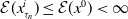 $\mathcal{E}({x}_{\tau _n}^i) \leq \mathcal{E}({x}^0) \lt \infty$
and thus
$\mathcal{E}({x}_{\tau _n}^i) \leq \mathcal{E}({x}^0) \lt \infty$
and thus
 $K$
is a
$K$
is a
 $d$
-bounded set, contained in sublevels of
$d$
-bounded set, contained in sublevels of
 $\mathcal{E}$
. Using relative compactness, i.e., Assumption 1.b, this ensures that
$\mathcal{E}$
. Using relative compactness, i.e., Assumption 1.b, this ensures that
 $\overline {K}$
is a
$\overline {K}$
is a
 $\sigma$
-sequentially compact set and therefore fulfils 1 of Proposition B.1. In order to apply the latter, it remains to choose a function
$\sigma$
-sequentially compact set and therefore fulfils 1 of Proposition B.1. In order to apply the latter, it remains to choose a function
 $\omega$
that fulfils 2. For this, we consider the sequence of curves
$\omega$
that fulfils 2. For this, we consider the sequence of curves
 $\left |{x}'_{\tau _n}\right |\;:\;[0,T]\to {\mathbb{R}}$
, which is by definition bounded in
$\left |{x}'_{\tau _n}\right |\;:\;[0,T]\to {\mathbb{R}}$
, which is by definition bounded in
 $L^\infty (0,T)$
, i.e.,
$L^\infty (0,T)$
, i.e.,
 \begin{equation*}\left \|\left |{x}'_{\tau _n}\right |\right \|_{L^\infty (0,T)}\leq 1, \qquad \text{for every }n\in \mathbb{N}.\end{equation*}
For fixed
 $0\leq s \leq t \leq T$
, let us define
$0\leq s \leq t \leq T$
, let us define
 \begin{align} s(n)\;:\!=\; \min _{k\in \{0,\ldots , n\}} \{ k\cdot \tau _n \,:\, s \leq k\cdot \tau _n \},\qquad t(n)\;:\!=\; \min _{k\in \{0,\ldots , n\}} \{ k\cdot \tau _n \,:\, t \leq k\cdot \tau _n \}. \end{align}
Using the triangle inequality and the fact that the distance between two consecutive iterates is bounded by
 $\tau$
, we obtain
$\tau$
, we obtain
 \begin{align} \limsup _{n\rightarrow +\infty } d(\bar {x}_{\tau _n}(s),\bar {x}_{\tau _n}(t)) &\leq \limsup _{n\rightarrow +\infty } \sum _{i=1}^{\frac {t(n)-s(n)}{\tau _n}} d(\bar {x}_{\tau _n}(s(n)+(i-1)\tau ),\bar {x}_{\tau _n}(s(n)+i\tau _n)) \end{align}
 \begin{align} &\leq \lim _{n\rightarrow +\infty } (t(n)-s(n))=|t-s |\;=\!:\; \omega (s,t). \end{align}
Therefore, 2 in Proposition B.1 is fulfilled, allowing us to apply [Reference Ambrosio, Gigli and Savaré2, Proposition 3.3.1] to extract another subsequence such that
 \begin{align*} \bar {x}_{\tau _n}(t) \stackrel {\sigma }{\rightharpoonup }u(t) \text{ as } n\rightarrow \infty \quad \forall t\in [0,T], \quad u \text{ is } d\text{-continuous in } [0,T]. \end{align*}
This in particular ensures
 $u(0)={x}^0$
and (2.12) together with Assumption 1.a yields 1-Lipschitzness of
$u(0)={x}^0$
and (2.12) together with Assumption 1.a yields 1-Lipschitzness of
 $u$
, since for
$u$
, since for
 $s\leq t$
, we have
$s\leq t$
, we have
 \begin{align*} d(u(s), u(t)) \leq \liminf _{n\to \infty } d(\bar {x}_{\tau _n}(s),\bar {x}_{\tau _n}(t))\leq t-s. \end{align*}
By construction, it holds that
 $d(\bar {x}_{\tau _n},\tilde {x}_{\tau _n})\leq \tau$
, which also yields
$d(\bar {x}_{\tau _n},\tilde {x}_{\tau _n})\leq \tau$
, which also yields
 \begin{align*} \tilde {x}_{\tau _n}(t) \stackrel {\sigma }{\rightharpoonup }u(t) \text{ as } n\rightarrow \infty \quad \forall t\in [0,T]. \end{align*}
Observing that
 $\tilde {x}_{\tau _n}(0)=x^0=u(0)$
independent of
$\tilde {x}_{\tau _n}(0)=x^0=u(0)$
independent of
 $n$
, we take the limes inferior for (2.9) and use Assumption 2.a and Fatou’s lemma to obtain for all
$n$
, we take the limes inferior for (2.9) and use Assumption 2.a and Fatou’s lemma to obtain for all
 $t\in [0,T]$
 \begin{align*} \mathcal{E}(u(0))&\geq \liminf _{n\rightarrow \infty } \left \{\mathcal{E}(\tilde {x}_{\tau _n}(t))-\int _0^t D_{\tau _n}(r)\,\text{d}r \right \} \geq \mathcal{E}(u(t))+\int _0^t \liminf _{n\rightarrow \infty } -D_{\tau _n}(r)\,\text{d}r\\ &\geq \mathcal{E}(u(t)) +\int _0^t |\partial \mathcal{E}(u(r))|\,\text{d}r. \end{align*}
The last inequality follows by the estimate
 \begin{align*} |\partial \mathcal{E}|(u(t))\leq \liminf _{n\rightarrow \infty } |\partial \mathcal{E}|(\tilde {x}_{\tau _n}(t))\leq \liminf _{n\rightarrow \infty } -D_{\tau _n}(t)\quad \text{ for a.e.}\quad t\in (0,T), \end{align*}
which is a consequence of (2.8) and (2.6) and the
 $\sigma$
-lower semicontinuity of the slope. On the other hand, we know that
$\sigma$
-lower semicontinuity of the slope. On the other hand, we know that
 $|\partial \mathcal{E}|$
is a strong upper gradient and
$|\partial \mathcal{E}|$
is a strong upper gradient and
 $|u'|(r)\leq 1$
for a.e.
$|u'|(r)\leq 1$
for a.e.
 $r \in [0,T]$
, such that
$r \in [0,T]$
, such that
 \begin{align*} \mathcal{E}(u(0))\leq \mathcal{E}(u(t))+\int _0^t |\partial \mathcal{E} |(u(r)) | u'|(r)\,\text{d}r\leq \mathcal{E}(u(t)) +\int _0^t |\partial \mathcal{E} |(u(r))\,\text{d}r. \end{align*}
In particular, the equality
 \begin{align*} \mathcal{E}(u(0))= \mathcal{E}(u(t))+\int _0^t |\partial \mathcal{E} |(u(r)) | u'|(r)\,\text{d}r= \mathcal{E}(u(t)) +\int _0^t |\partial \mathcal{E} |(u(r))\,\text{d}r \end{align*}
must hold. It follows that
 $t\mapsto \mathcal{E}(u(t))$
is locally absolutely continuous and
$t\mapsto \mathcal{E}(u(t))$
is locally absolutely continuous and
 \begin{align*} \frac {\text{d}}{\text{d}t}\mathcal{E}(u(t))=-|\partial \mathcal{E}|(u(t)) |u'|(t)=-|\partial \mathcal{E}|(u(t)) \text{ for a.e.}t\in (0,T). \end{align*}
3. Banach space setting
In this section, we consider the Banach space setting, i.e., we assume that
 $\mathcal{S}=\mathcal{X}$
, where
$\mathcal{S}=\mathcal{X}$
, where
 $\mathcal{X}$
is a Banach space with norm
$\mathcal{X}$
is a Banach space with norm
 $\|\cdot \|$
and
$\|\cdot \|$
and
 $(\mathcal{X}^*,\|\cdot \|_*)$
denoting its dual. In this section, we assume the functional to be a
$(\mathcal{X}^*,\|\cdot \|_*)$
denoting its dual. In this section, we assume the functional to be a
 $C^1$
-perturbation (see section 3.1) and use the symbol
$C^1$
-perturbation (see section 3.1) and use the symbol
 $E$
to distinguish it from general functionals
$E$
to distinguish it from general functionals
 $\mathcal{E}$
in the previous section. We want to give an equivalent characterization of curves of maximum slope in terms of differential inclusions. Following [Reference Ambrosio, Gigli and Savaré2, Ch. 1], for a functional
$\mathcal{E}$
in the previous section. We want to give an equivalent characterization of curves of maximum slope in terms of differential inclusions. Following [Reference Ambrosio, Gigli and Savaré2, Ch. 1], for a functional
 $E\;:\;\mathcal{X}\to ({-}\infty ,\infty ]$
, we employ the Fréchet subdifferential
$E\;:\;\mathcal{X}\to ({-}\infty ,\infty ]$
, we employ the Fréchet subdifferential
 $\partial E \subset \mathcal{X}^*$
, where for
$\partial E \subset \mathcal{X}^*$
, where for
 ${x}\in \operatorname {dom}(E)$
, we define
${x}\in \operatorname {dom}(E)$
, we define
 \begin{align} \xi \in \partial E ({x}) \Leftrightarrow \liminf _{z\to {x}} \frac {E (z) - E ({x}) - \langle \xi , z-{x}\rangle }{\|z-{x}\|}\geq 0 \end{align}
with
 $\operatorname {dom}(\partial E ) = \{{x}\in \mathcal{X}\,:\, \partial E ({x})\neq \emptyset \}$
. Assuming that
$\operatorname {dom}(\partial E ) = \{{x}\in \mathcal{X}\,:\, \partial E ({x})\neq \emptyset \}$
. Assuming that
 $\partial E ({x})$
is weakly
$\partial E ({x})$
is weakly
 $^*$
closed for every
$^*$
closed for every
 ${x}\in \operatorname {\operatorname {dom}}(\partial E )$
– which holds true in particular, if
${x}\in \operatorname {\operatorname {dom}}(\partial E )$
– which holds true in particular, if
 $\mathcal{X}$
is reflexive or
$\mathcal{X}$
is reflexive or
 $ E$
is a so called
$ E$
is a so called
 $C^1$
-perturbation of a convex function (see Proposition 3.1) – we furthermore define
$C^1$
-perturbation of a convex function (see Proposition 3.1) – we furthermore define
 \begin{align*} \partial ^\circ E ({x}) \;:\!=\; \operatorname*{arg\,min}_{\xi \in \partial E ({x})} \|\xi \|_*\subset \partial E ({x}). \end{align*}
Note that
 $\partial ^\circ E (x)$
is still potentially multivalued; however, all elements have the same dual norm. This justifies using the notation
$\partial ^\circ E (x)$
is still potentially multivalued; however, all elements have the same dual norm. This justifies using the notation
 $\left \|\partial ^\circ E (x)\right \|_*=\min \{\|\xi \|_*\,:\,\xi \in \partial E ({x})\}$
in the following.
$\left \|\partial ^\circ E (x)\right \|_*=\min \{\|\xi \|_*\,:\,\xi \in \partial E ({x})\}$
in the following.
3.1. On
$\boldsymbol{\boldsymbol{C}}^{\bf 1}$
-perturbations of convex functions

Functions that can be split into a convex function
 $ E ^{\mathrm{c}}$
and a differentiable part
$ E ^{\mathrm{c}}$
and a differentiable part
 $ E ^{\mathrm{d}}$
, i.e.,
$ E ^{\mathrm{d}}$
, i.e.,
 $ E = E ^{\mathrm{c}}+ E ^{\mathrm{d}}$
, are called
$ E = E ^{\mathrm{c}}+ E ^{\mathrm{d}}$
, are called
 $C^1$
-perturbations of convex functions. This particular class of functions exhibits a variety of useful properties. We collect the ones that are relevant for our setting in the following proposition, which is a combination of Corollary 1.4.5 and Lemma 2.3.6 in [Reference Ambrosio, Gigli and Savaré2].
$C^1$
-perturbations of convex functions. This particular class of functions exhibits a variety of useful properties. We collect the ones that are relevant for our setting in the following proposition, which is a combination of Corollary 1.4.5 and Lemma 2.3.6 in [Reference Ambrosio, Gigli and Savaré2].
Proposition 3.1 (
 $C^1$
-perturbations of convex functions). If
$C^1$
-perturbations of convex functions). If
 $E \;:\;\mathcal{X}\rightarrow ({-}\infty ,+\infty ]$
admits a decomposition
$E \;:\;\mathcal{X}\rightarrow ({-}\infty ,+\infty ]$
admits a decomposition
 $ E = E ^{\mathrm{c}}+ E ^{\mathrm{d}}$
, into a proper, lower semicontinuous convex function
$ E = E ^{\mathrm{c}}+ E ^{\mathrm{d}}$
, into a proper, lower semicontinuous convex function
 $ E ^{\mathrm{c}}$
and a
$ E ^{\mathrm{c}}$
and a
 $C^1$
-function
$C^1$
-function
 $ E ^{\mathrm{d}}$
, then
$ E ^{\mathrm{d}}$
, then
-
(i)
$\partial E =\partial E ^{\mathrm{c}}+D E ^{\mathrm{d}}$
, -
(ii)
\begin{align*} \left . \begin{aligned} \xi ^{ n}\in \partial E({x}^{n}),\\ {x}^{n}\to {x}\in \operatorname {dom}(\partial E),\\ \xi ^{n} \rightharpoonup ^* \xi \end{aligned}\right \}\Rightarrow \left \{\begin{aligned}\xi \in \partial E({x}),\\ E ({x}^{n})\to E ({x}), \end{aligned}\right . \end{align*}
-
(iii)
$|\partial E |({x})=\|\partial ^\circ E ({x})\|_* \quad \forall {x}\in \mathcal{X},$
-
(iv)
$|\partial E |$
is
$\|\cdot \|$
-lower semicontinuous,
-
(v)
$|\partial E |$
is a strong upper gradient of
$ E$
.


Considering Banach spaces that fulfil Assumptions 1.a and 1.b with their strong topology and energies that are
 $C^1$
perturbations, the existence of
$C^1$
perturbations, the existence of
 $\infty$
-curves of maximum slope follows directly by Theorem 2.11.
$\infty$
-curves of maximum slope follows directly by Theorem 2.11.
An important example of such a Banach space
 $\mathcal{X}$
is the Euclidean space, since our motivating application, namely adversarial attacks, usually employs a finite-dimensional image space. We formulate this result in the following corollary.
$\mathcal{X}$
is the Euclidean space, since our motivating application, namely adversarial attacks, usually employs a finite-dimensional image space. We formulate this result in the following corollary.
Corollary 3.2 (Existence for
 $C^1$
-perturbations in finite dimensions). Let
$C^1$
-perturbations in finite dimensions). Let
 $\mathcal{X}=(\mathbb{R}^d,\|\cdot \|)$
and
$\mathcal{X}=(\mathbb{R}^d,\|\cdot \|)$
and
 $E \;:\;\mathbb{R}^d\rightarrow ({-}\infty ,+\infty ]$
admit a decomposition
$E \;:\;\mathbb{R}^d\rightarrow ({-}\infty ,+\infty ]$
admit a decomposition
 $ E = E ^{\mathrm{c}}+ E ^{\mathrm{d}}$
into a proper, lower semicontinuous convex function
$ E = E ^{\mathrm{c}}+ E ^{\mathrm{d}}$
into a proper, lower semicontinuous convex function
 $ E ^{\mathrm{c}}$
and a
$ E ^{\mathrm{c}}$
and a
 $C^1$
-function
$C^1$
-function
 $ E ^{\mathrm{d}}$
. For every
$ E ^{\mathrm{d}}$
. For every
 ${x}^0\in \operatorname {dom}( E )$
, there exists at least one curve of maximal slope in the sense of Definition 2.1 with
${x}^0\in \operatorname {dom}( E )$
, there exists at least one curve of maximal slope in the sense of Definition 2.1 with
 $u(0)={x}^0$
. Further, this curve satisfies the energy dissipation equality (2.10).
$u(0)={x}^0$
. Further, this curve satisfies the energy dissipation equality (2.10).
Proof. We choose
 $\sigma$
to be the norm topology, such that Assumptions 1.a and 1.b are fulfilled and
$\sigma$
to be the norm topology, such that Assumptions 1.a and 1.b are fulfilled and
 $ E$
fulfils Assumption 2.a. By Proposition 3.1,
$ E$
fulfils Assumption 2.a. By Proposition 3.1,
 $\left |\partial E \right |$
is lower semicontinuous and a strong upper gradient. Therefore, also Assumption 2.b is fulfilled and the application of Theorem 2.11 yields the desired result.
$\left |\partial E \right |$
is lower semicontinuous and a strong upper gradient. Therefore, also Assumption 2.b is fulfilled and the application of Theorem 2.11 yields the desired result.
In the infinite-dimensional case, existence is harder to prove. Usually,
 $\sigma$
is chosen as the weak or weak* topology, such that when
$\sigma$
is chosen as the weak or weak* topology, such that when
 $\mathcal{X}$
is reflexive or a dual space, the Banach–Alaoglu theorem yields compactness and that Assumptions 1.a and 1.b are fulfilled. A desirable property for the energy functional is the so-called
$\mathcal{X}$
is reflexive or a dual space, the Banach–Alaoglu theorem yields compactness and that Assumptions 1.a and 1.b are fulfilled. A desirable property for the energy functional is the so-called
 $\sigma$
-weak* closure property
$\sigma$
-weak* closure property
 \begin{align*} \left .\begin{aligned}\xi ^{n}\in \partial E({x}^{n}),\\ {x}^{n} \stackrel {\sigma }{\to } {x}\in \operatorname {dom}(\partial E),\\ \xi ^{n} \rightharpoonup ^* \xi \end{aligned}\right \} \Rightarrow \left \{\begin{aligned}\xi \in \partial E({x}),\\ E ({x}^{n})\to E ({x}) \end{aligned}\right . \end{align*}
of its subdifferential, c.f. Item 2. The
 $\sigma$
-lower semicontinuity of the slope Assumption 2.b and (3.7) are almost immediate consequences of the closure property, as was shown in [Reference Ambrosio, Gigli and Savaré2, Lemma 2.3.6, Theorem 2.3.8].
$\sigma$
-lower semicontinuity of the slope Assumption 2.b and (3.7) are almost immediate consequences of the closure property, as was shown in [Reference Ambrosio, Gigli and Savaré2, Lemma 2.3.6, Theorem 2.3.8].
Example 2.
As an application of Corollary 3.2
, we consider the finite-dimensional adversarial setting introduced in section 1
, i.e., we choose
 $\mathcal{X}={\mathbb{R}}^d$
. Let
$\mathcal{X}={\mathbb{R}}^d$
. Let
 \begin{align*} E ({x})\;:\!=\; \underbrace {-\ell (h({x}),y)}_{= E ^{\mathrm{d}}} + \underbrace {\chi _{\overline {B_\varepsilon }({x}^0)}}_{E^{\mathrm{c}}} , \end{align*}
then by the chain rule
 $E^{\mathrm{d}}\in C^1(\mathcal{X})$
, if
$E^{\mathrm{d}}\in C^1(\mathcal{X})$
, if
 $h\in C^1(\mathcal{X};\mathcal{Y})$
and
$h\in C^1(\mathcal{X};\mathcal{Y})$
and
 $\ell \in C^1(\mathcal{Y}\times \mathcal{Y})$
. We consider a neural network
$\ell \in C^1(\mathcal{Y}\times \mathcal{Y})$
. We consider a neural network
 $h = \phi ^L\circ \ldots \circ \phi ^1$
with the
$h = \phi ^L\circ \ldots \circ \phi ^1$
with the
 $l$
th layer being given as
$l$
th layer being given as
 \begin{align*} \phi ^l\;:\;{\mathbb{R}}^{d^l}\to {\mathbb{R}}^{d^{l+1}}, \phi ^l(z)\;:\!=\; \alpha (W z + b), \end{align*}
for a weight matrix
 $W\in {\mathbb{R}}^{d^{l+1}, d^l}$
, bias
$W\in {\mathbb{R}}^{d^{l+1}, d^l}$
, bias
 $b\in {\mathbb{R}}^{d^{l+1}}$
and activation function
$b\in {\mathbb{R}}^{d^{l+1}}$
and activation function
 $\alpha \;:\;{\mathbb{R}}\to {\mathbb{R}}$
, which is applied entry-wise. Therefore, the network
$\alpha \;:\;{\mathbb{R}}\to {\mathbb{R}}$
, which is applied entry-wise. Therefore, the network
 $h$
is
$h$
is
 $C^1$
if its activation function is in
$C^1$
if its activation function is in
 $C^1({\mathbb{R}})$
. Typical examples that fulfil this assumption are the Sigmoid function and smooth approximations to ReLU [42], such as GeLU [51], see also Appendix H for more details on such activation functions. Furthermore, many popular loss functions are in
$C^1({\mathbb{R}})$
. Typical examples that fulfil this assumption are the Sigmoid function and smooth approximations to ReLU [42], such as GeLU [51], see also Appendix H for more details on such activation functions. Furthermore, many popular loss functions are in
 $C^1(\mathcal{Y}\times \mathcal{Y})$
, like the mean squared error (MSE) or Cross-Entropy paired with a Softmax layer [Reference Boltzmann9, Reference Cybenko, O’Leary and Rissanen29, Reference Good45]. On the other hand, the root MSE is not differentiable whenever a component is
$C^1(\mathcal{Y}\times \mathcal{Y})$
, like the mean squared error (MSE) or Cross-Entropy paired with a Softmax layer [Reference Boltzmann9, Reference Cybenko, O’Leary and Rissanen29, Reference Good45]. On the other hand, the root MSE is not differentiable whenever a component is
 $0$
.
$0$
.
Lemma 2.8 provides an alternative characterization of the metric slope, employing a
 $\limsup$
formulation. The next two lemmas show that
$\limsup$
formulation. The next two lemmas show that
 $C^1$
-perturbations are regular enough, such that the limit superior can be replaced by a standard limit. This is used in Lemma 4.17. The first lemma establishes the fact that for convex functionals, there is a minimizing sequence for the value of
$C^1$
-perturbations are regular enough, such that the limit superior can be replaced by a standard limit. This is used in Lemma 4.17. The first lemma establishes the fact that for convex functionals, there is a minimizing sequence for the value of
 $E_\tau ({x})$
that lies on the boundary
$E_\tau ({x})$
that lies on the boundary
 $\partial B_\tau ({x})$
.
$\partial B_\tau ({x})$
.
Remark 3.3. Similar to [Reference Ambrosio, Gigli and Savaré2, section 3.1], we remark some properties of
 $E_\tau (x)=\inf _{\tilde {{x}}\in \overline {B_\tau }(x)}E(\tilde {{x}})$
in the case, when
$E_\tau (x)=\inf _{\tilde {{x}}\in \overline {B_\tau }(x)}E(\tilde {{x}})$
in the case, when
 $E$
is convex. Since
$E$
is convex. Since
 $E_\tau (x)$
is defined via the infimal convolution, see Remark 2.6, we can directly infer convexity in the
$E_\tau (x)$
is defined via the infimal convolution, see Remark 2.6, we can directly infer convexity in the
 $x$
argument, if
$x$
argument, if
 $E$
was already convex. Furthermore, we also have convexity in
$E$
was already convex. Furthermore, we also have convexity in
 $\tau$
, which can be seen as follows. Let
$\tau$
, which can be seen as follows. Let
 $\tau _1,\tau _2\geq 0$
be arbitrary, where we also allow them to attain
$\tau _1,\tau _2\geq 0$
be arbitrary, where we also allow them to attain
 $0$
. For any
$0$
. For any
 $z_1\in \overline {B_{\tau _1}}(x), z_2\in \overline {B_{\tau _2}}(x)$
, we have that
$z_1\in \overline {B_{\tau _1}}(x), z_2\in \overline {B_{\tau _2}}(x)$
, we have that
 $\lambda z_1 + (1-\lambda ) z_2 \in \overline {B_{\tilde {\tau }}}(x)$
with
$\lambda z_1 + (1-\lambda ) z_2 \in \overline {B_{\tilde {\tau }}}(x)$
with
 $\tilde {\tau }=\lambda \tau _1 + (1-\lambda )\tau _2$
for any
$\tilde {\tau }=\lambda \tau _1 + (1-\lambda )\tau _2$
for any
 $\lambda \in [0,1]$
. The definition of
$\lambda \in [0,1]$
. The definition of
 $E_\tau$
and the convexity of
$E_\tau$
and the convexity of
 $E$
yield
$E$
yield
 \begin{align*} E_{\tilde {\tau }}(x)\leq E (\lambda z_1 + (1-\lambda ) z_2) \leq \lambda E (z_1) + (1-\lambda ) E (z_2) \end{align*}
and since
 $z_1\in \overline {B_{\tau _1}}(x), z_2\in \overline {B_{\tau _2}}(x)$
were arbitrary, we obtain
$z_1\in \overline {B_{\tau _1}}(x), z_2\in \overline {B_{\tau _2}}(x)$
were arbitrary, we obtain
 \begin{align*} E_{\tilde {\tau }}(x)\leq \lambda E_{\tau _1}(x) + (1-\lambda ) E_{\tau _2}(x). \end{align*}
If
 $x\in \operatorname {dom}(E))$
, we have that
$x\in \operatorname {dom}(E))$
, we have that
 $\operatorname {dom}(\tau \mapsto E_\tau (x))=[0,\infty )$
and thus
$\operatorname {dom}(\tau \mapsto E_\tau (x))=[0,\infty )$
and thus
 $\tau \to E_\tau$
is continous on
$\tau \to E_\tau$
is continous on
 $(0,\infty )$
. If
$(0,\infty )$
. If
 $ E$
is lower semicontinuous, we also obtain continuity at
$ E$
is lower semicontinuous, we also obtain continuity at
 $0$
.
$0$
.
Lemma 3.4.
If
 $E$
is a proper, convex, lower semicontinuous function, then for all
$E$
is a proper, convex, lower semicontinuous function, then for all
 $x\in \operatorname {dom}(E)$
with
$x\in \operatorname {dom}(E)$
with
 $|\partial E ({x})|\not = 0$
, there is an
$|\partial E ({x})|\not = 0$
, there is an
 $\epsilon \gt 0$
such that for all
$\epsilon \gt 0$
such that for all
 $0\lt \tau \lt \epsilon$
, there exists a sequence
$0\lt \tau \lt \epsilon$
, there exists a sequence
 $\left ({x}^{n}\right )_{n\in \mathbb{N}}$
with
$\left ({x}^{n}\right )_{n\in \mathbb{N}}$
with
 \begin{align} E ({x}^{n})\rightarrow E _{\tau }({x})\quad and \quad \|{x}-{x}^{n}\|=\tau \ \forall n\in \mathbb{N}. \end{align}
If in addition the Banach space
 $\mathcal{X}$
is reflexive, then there exists
$\mathcal{X}$
is reflexive, then there exists
 ${x}_\tau \in \mathcal{X}$
with
${x}_\tau \in \mathcal{X}$
with
 \begin{align*} E ({x}_\tau )= E _{\tau }({x})\quad and \quad \|{x}-{x}_\tau \|=\tau . \end{align*}
Proof. Let
 ${x}\in \operatorname {dom}(E)$
with
${x}\in \operatorname {dom}(E)$
with
 $|\partial E({x})|\not = 0$
, then the mapping
$|\partial E({x})|\not = 0$
, then the mapping
 $\tau \mapsto E _\tau ({x})$
is non-increasing and not constant. Therefore, we can find an
$\tau \mapsto E _\tau ({x})$
is non-increasing and not constant. Therefore, we can find an
 $\epsilon \gt 0$
such that
$\epsilon \gt 0$
such that
 $E_\tau ({x})\gt E_{\epsilon }({x})$
for all
$E_\tau ({x})\gt E_{\epsilon }({x})$
for all
 $0\lt \tau \lt \epsilon$
. Let
$0\lt \tau \lt \epsilon$
. Let
 $\left (\tilde {{x}}^{n}\right )_{n\in \mathbb{N}}$
be a sequence such that
$\left (\tilde {{x}}^{n}\right )_{n\in \mathbb{N}}$
be a sequence such that
 \begin{align*} \lim _{n\to \infty } E (\tilde {{x}}_n) = E _\tau ({x}). \end{align*}
Since
 $ E_\tau ({x})\gt E _{\epsilon }({x})$
, we can find an element
$ E_\tau ({x})\gt E _{\epsilon }({x})$
, we can find an element
 $\hat {{x}}$
that fulfils
$\hat {{x}}$
that fulfils
 \begin{align*} E (\tilde {{x}}_n)\gt E (\hat {{x}})\qquad \text{for every } n\in \mathbb{N}\qquad \text{and}\qquad \tau \lt \left \|{x}- \hat {{x}}\right \| \leq {\epsilon }. \end{align*}
Since
 $\hat {{x}}\notin \overline {B_\tau }({x})$
and
$\hat {{x}}\notin \overline {B_\tau }({x})$
and
 $\tilde {{x}}_n\in \overline {B_\tau }({x})$
, the line between each pair
$\tilde {{x}}_n\in \overline {B_\tau }({x})$
, the line between each pair
 $(\hat {{x}}, \tilde {{x}}_n)$
,
$(\hat {{x}}, \tilde {{x}}_n)$
,
 \begin{align*} c_n\;:\;t\in [0,1]\mapsto t\hat {{x}}+(1-t)\tilde {{x}}_n \end{align*}
has to intersect the sphere
 $\partial B_\tau ({x})$
at some point
$\partial B_\tau ({x})$
at some point
 $t_n\in [0,1)$
, where we define the intersection point as
$t_n\in [0,1)$
, where we define the intersection point as
 ${x}_n=c_n(t_n)\in \partial B_\tau ({x})$
. Due to convexity, we obtain
${x}_n=c_n(t_n)\in \partial B_\tau ({x})$
. Due to convexity, we obtain
 \begin{align*} E _\tau ({x}) \leq E ({x}_n) = E (t_n\hat {{x}}+(1-t_n)\tilde {{x}}_n)\leq t_n E (\hat {{x}}) + (1-t_n) E (\tilde {{x}}_n) \leq E (\tilde {{x}}_n). \end{align*}
Note that the last inequality would only be strict if
 $t_n\neq 0$
; however, since
$t_n\neq 0$
; however, since
 $\tilde {{x}}_n$
might already be lying on the sphere, we only obtain the weak inequality. The sequence
$\tilde {{x}}_n$
might already be lying on the sphere, we only obtain the weak inequality. The sequence
 ${x}_n$
now is the desired sequence in (3.2).
${x}_n$
now is the desired sequence in (3.2).
In the reflexive case, the weak compactness of the unit ball guarantees weak convergence of a subsequence of
 $\left ({x}^{n}\right )_{n\in \mathbb{N}}$
to some
$\left ({x}^{n}\right )_{n\in \mathbb{N}}$
to some
 ${x}_\tau \in \overline {B_\tau }({x})$
. Lower semicontinuity and convexity imply weak lower semicontinuity of
${x}_\tau \in \overline {B_\tau }({x})$
. Lower semicontinuity and convexity imply weak lower semicontinuity of
 $ E$
and thus
$ E$
and thus
 \begin{align*} E _\tau ({x})\leq E ({x}_\tau ) \leq \liminf _{n\to \infty } E ({x}_n) = E _\tau ({x}). \end{align*}
As above, we can choose an element
 $\hat {x}$
with
$\hat {x}$
with
 $\left \|\hat {x} - x\right \|\gt \tau$
with
$\left \|\hat {x} - x\right \|\gt \tau$
with
 $E(x_\tau ) \gt E (\hat {x})$
. Applying the same argument as above, there is some
$E(x_\tau ) \gt E (\hat {x})$
. Applying the same argument as above, there is some
 $t\in [0,1)$
such that
$t\in [0,1)$
such that
 $t\hat {x} + (1-t) x_\tau$
intersects
$t\hat {x} + (1-t) x_\tau$
intersects
 $\partial B_\tau (x)$
. As above, if
$\partial B_\tau (x)$
. As above, if
 $t\neq 0$
, convexity yields
$t\neq 0$
, convexity yields
 \begin{align} E _\tau ({x})\leq E (t\hat {x} + (1-t) x_\tau ) \lt E (x_\tau ), \end{align}
which contradicts the fact that
 $ E_\tau ({x})= E (x_\tau )$
and thus
$ E_\tau ({x})= E (x_\tau )$
and thus
 $x_\tau$
must have already been on the boundary.
$x_\tau$
must have already been on the boundary.
Using the previous lemma, we can now show that for
 $C^1$
-perturbations of convex functions, we can replace the
$C^1$
-perturbations of convex functions, we can replace the
 $\limsup$
in Lemma 2.8 by a normal limit.
$\limsup$
in Lemma 2.8 by a normal limit.
Lemma 3.5.
Let
 $ E \;:\;\mathcal{X}\rightarrow ({-}\infty ,+\infty ]$
admit a decomposition
$ E \;:\;\mathcal{X}\rightarrow ({-}\infty ,+\infty ]$
admit a decomposition
 $ E = E ^{\mathrm{c}}+ E ^{\mathrm{d}}$
, into a proper, lower semicontinuous convex function
$ E = E ^{\mathrm{c}}+ E ^{\mathrm{d}}$
, into a proper, lower semicontinuous convex function
 $E ^{\mathrm{c}}$
and a
$E ^{\mathrm{c}}$
and a
 $C^1$
-function
$C^1$
-function
 $ E ^{\mathrm{d}}$
, then for all
$ E ^{\mathrm{d}}$
, then for all
 $x\in \operatorname {dom}( E )$
, we have
$x\in \operatorname {dom}( E )$
, we have
 \begin{align} |\partial E |({x})=\lim _{\tau \rightarrow 0^+}\frac { E ({x})- E _\tau ({x})}{\tau }. \end{align}
Proof. Step 1: The convex case.
We first assume that
 $E$
is convex. We choose
$E$
is convex. We choose
 $\tau$
small enough such that by Lemma 3.4, we obtain a sequence
$\tau$
small enough such that by Lemma 3.4, we obtain a sequence
 $\{{x}_n\}_n$
with
$\{{x}_n\}_n$
with
 $\|{x}-{x}_n\|=\tau$
and
$\|{x}-{x}_n\|=\tau$
and
 $\lim _{n\to \infty } E ({x}_n) = E _\tau ({x})$
. For each
$\lim _{n\to \infty } E ({x}_n) = E _\tau ({x})$
. For each
 $n\in \mathbb{N}$
, we consider the line
$n\in \mathbb{N}$
, we consider the line
 \begin{align*} c_n(t)\;:\!=\; t\, {x}_n + (1-t)\, {x} \end{align*}
evaluated at
 $\tilde {t}=\tilde {\tau }/\tau$
for some
$\tilde {t}=\tilde {\tau }/\tau$
for some
 $0\lt \tilde {\tau }\lt \tau$
, which yields
$0\lt \tilde {\tau }\lt \tau$
, which yields
 $\left \|{x}-c_n(\tilde {t})\right \|=\tilde {\tau }/\tau \left \|{x}-{x}_n\right \| = \tilde {\tau }$
. Due to convexity, we obtain
$\left \|{x}-c_n(\tilde {t})\right \|=\tilde {\tau }/\tau \left \|{x}-{x}_n\right \| = \tilde {\tau }$
. Due to convexity, we obtain
 \begin{align*} E (c_n(\tilde {t})) \leq \tilde {t}\, E ({x}_n)+\left (1-\tilde {t}\right )\, E ({x})\qquad \Rightarrow \qquad E ({x}) - E (c_n(\tilde {t})) \geq \tilde {t}\, \left ( E ({x}) - E ({x}_n)\right ). \end{align*}
Using the fact that
 $ E _{\tilde {\tau }}({x}) \leq E (c_n(\tilde {t}))$
and dividing by
$ E _{\tilde {\tau }}({x}) \leq E (c_n(\tilde {t}))$
and dividing by
 $\tilde {\tau }$
in the above inequality yields
$\tilde {\tau }$
in the above inequality yields
 \begin{align*} \frac {E ({x})- E _{\tilde {\tau }}({x})}{\tilde {\tau }}\geq \frac { E ({x})- E (c_n(\tilde {t}))}{\tilde {\tau }} \geq \frac { E ({x})- E ({x}_n)}{\tau }. \end{align*}
Considering the limit
 $n\to \infty$
, we obtain the following inequality,
$n\to \infty$
, we obtain the following inequality,
 \begin{align*} \frac {E({x})-E_{\tilde {\tau }}({x})}{\tilde {\tau }}\geq \limsup _{n\rightarrow \infty }\frac { E ({x})- E (c_n(\tilde {t}))}{\tilde {\tau }}\geq \lim _{n\rightarrow \infty }\frac {E({x})-E({x}_n)}{\tau }=\frac {E({x})-E_\tau ({x})}{\tau }. \end{align*}
This shows that
 $\tau \mapsto Q(\tau ) \;:\!=\; \frac {E({x})-E_\tau ({x})}{\tau }$
is decreasing in
$\tau \mapsto Q(\tau ) \;:\!=\; \frac {E({x})-E_\tau ({x})}{\tau }$
is decreasing in
 $\tau$
, and therefore, for a null sequence
$\tau$
, and therefore, for a null sequence
 $\tau _n\to 0$
,
$\tau _n\to 0$
,
 $Q(\tau _n)$
is an increasing sequence. The monotone convergence theorem together with Lemma 2.8 shows (3.4).
$Q(\tau _n)$
is an increasing sequence. The monotone convergence theorem together with Lemma 2.8 shows (3.4).
Step 2: Extension to
 $C^1$
-perturbations.
$C^1$
-perturbations.
We now assume that
 $E$
is a
$E$
is a
 $C^1$
-perturbation of a convex function. By the definition of differentiability, we can write
$C^1$
-perturbation of a convex function. By the definition of differentiability, we can write
 \begin{align*} E (z)=\underbrace { E ^{\mathrm{c}}(z)+ E ^{\mathrm{d}}({x})-\langle D E ^{\mathrm{d}}({x}),{x}-z\rangle }_{\;=\!:\; F ({x})}+R({x},{x}-z), \end{align*}
with
 $R({x},{x}-z)\in o(|{x}-z|)$
for every
$R({x},{x}-z)\in o(|{x}-z|)$
for every
 $z\in \operatorname {dom}( E )$
. We observe that
$z\in \operatorname {dom}( E )$
. We observe that
 $ F$
is again a convex function. Let
$ F$
is again a convex function. Let
 $\epsilon \gt 0$
, then we denote by
$\epsilon \gt 0$
, then we denote by
 ${x} ^{ E }_{\tau ,\epsilon },{x}^{ F }_{\tau ,\epsilon }\in \overline {B_\tau }({x})$
the quasi-minimizers that fulfil
${x} ^{ E }_{\tau ,\epsilon },{x}^{ F }_{\tau ,\epsilon }\in \overline {B_\tau }({x})$
the quasi-minimizers that fulfil
 \begin{align*} E ({x}^{ E }_{\tau ,\epsilon })- E_{\tau }({x})\leq \tau \epsilon \quad \text{and}\quad F ({x}^{F}_{\tau ,\epsilon })- F_{\tau }({x})\leq \tau \epsilon \quad \text{respectively}. \end{align*}
We use the estimate
 \begin{gather*} E _{\tau }({x})- F _{\tau }({x})\leq E _{\tau }({x}) - F ({x}^{ F }_{\tau ,\epsilon }) + \tau \epsilon \\ =\underbrace {E _{\tau }({x})- E ({x}^{ F }_{\tau ,\epsilon })}_{\leq 0} + R({x},{x}-{x}^{ F }_{\tau ,\epsilon })+ \tau \epsilon \leq |R({x},{x}-{x}^{ F }_{\tau ,\epsilon })|+\tau \epsilon \end{gather*}
and analogously
 \begin{gather*} F _{\tau }({x})- E _{\tau }({x})\leq F _{\tau }({x})- E ({x}^{E }_{\tau ,\epsilon }) + \tau \epsilon \\ =\underbrace {F _{\tau }({x})- F ({x}^{ E }_{\tau ,\epsilon })}_{\leq 0}-R({x},{x}-{x}^{ E }_{\tau ,\epsilon })+\tau \epsilon \leq |R({x},{x}-{x}^{E}_{\tau ,\epsilon })|+\tau \epsilon , \end{gather*}
to obtain
 \begin{align} |E_{\tau }({x})-F_{\tau }({x})|\leq \max \left \{ |R({x},{x}-{x}^{E}_{\tau ,\epsilon })|, |R({x},{x}-{x}^{F}_{\tau ,\epsilon })|\right \}+\tau \epsilon . \end{align}
Using that
 $ E ({x}) =F ({x})$
and dividing by
$ E ({x}) =F ({x})$
and dividing by
 $\tau$
in (3.5) yields the inequality
$\tau$
in (3.5) yields the inequality
 \begin{gather} \left |\frac {E({x})-E_{\tau }({x})}{\tau }-\frac {F({x})-F_{\tau }({x})}{\tau } \right |\leq \underbrace {\frac {\max \{ |R({x},{x}-{x}^{ E }_{\tau }(\epsilon ))|, |R({x},{x}-{x}^{ F }_{\tau }(\epsilon ))|\}}{\tau }}_{\;:\!=\;r(\tau )}+\epsilon . \end{gather}
Since
 $\left |{x}-{x}^{E}_\tau (\epsilon )\right |= \left |{x}-{x}^{F}_\tau (\epsilon )\right |\leq \tau$
, it holds
$\left |{x}-{x}^{E}_\tau (\epsilon )\right |= \left |{x}-{x}^{F}_\tau (\epsilon )\right |\leq \tau$
, it holds
 $\lim _{\tau \to 0} r(\tau ) = 0$
. Taking the
$\lim _{\tau \to 0} r(\tau ) = 0$
. Taking the
 $\limsup$
of (3.6) and sending
$\limsup$
of (3.6) and sending
 $\epsilon$
to zero then yields,
$\epsilon$
to zero then yields,
 \begin{align*} \lim _{\tau \to 0^+} \left |\frac {E({x})-E_{\tau }({x})}{\tau }-\frac {F({x})-F_{\tau }({x})}{\tau } \right | = 0. \end{align*}
Therefore, the limit in (3.4) exists,
 \begin{align*} \lim _{\tau \to 0^+} \frac {E({x})-E_{\tau }({x})}{\tau } &=\lim _{\tau \to 0^+} \frac {E({x})-E_{\tau }({x})}{\tau }-\frac {F({x})-F_{\tau }({x})}{\tau } + \frac {F({x})-F_{\tau }({x})}{\tau }\\ &=\lim _{\tau \to 0^+} \frac {F({x})-F_{\tau }({x})}{\tau }=\left |\partial F\right |({x}), \end{align*}
where in the last step, we used that
 $F$
is convex together with Step 1.
$F$
is convex together with Step 1.
3.2. Differential inclusions
Similar to [Reference Ambrosio, Gigli and Savaré2, Proposition 1.4.1] for finite
 $p$
, we now give a characterization of
$p$
, we now give a characterization of
 $\infty$
-curves of maximal slope via differential inclusions, whenever the slope of the energy
$\infty$
-curves of maximal slope via differential inclusions, whenever the slope of the energy
 $ E$
can be written as
$ E$
can be written as
 \begin{align} |\partial E |({x})=\min \{\|\xi \|_*\,:\,\xi \in \partial E ({x})\}=\|\partial ^\circ E ({x})\|_* \quad \forall {x}\in \mathcal{X}. \end{align}
By Proposition 3.1, this is, e.g., the case for
 $C^1$
-perturbations. Let us start by defining a degenerate duality mapping
$C^1$
-perturbations. Let us start by defining a degenerate duality mapping
 $\mathcal{J}_\infty : \mathcal{X} \rightarrow 2^{\mathcal{X}^*}$
,
$\mathcal{J}_\infty : \mathcal{X} \rightarrow 2^{\mathcal{X}^*}$
,
 \begin{align*} \mathcal{J}_\infty ({x})\;:\!=\; \begin{cases} \{\xi \in \mathcal{X}^*\,:\, \langle \xi ,u\rangle =\| \xi \|_*\} &\text{if } \|{x}\|=1,\\ \{0\} &\text{if } \|{x}\|\lt 1,\\ \emptyset &\text{if } \|{x}\|\gt 1, \end{cases} \end{align*}
as the limit case of the classical
 $p$
-duality mapping [Reference Schuster, Kaltenbacher, Hofmann and Kazimierski93, Definition 2.27]
$p$
-duality mapping [Reference Schuster, Kaltenbacher, Hofmann and Kazimierski93, Definition 2.27]
 \begin{align*} \mathcal{J}_p({x})\;:\!=\; \left \{ \zeta \in \mathcal{X}^*\,:\, \ \langle \zeta , u \rangle =\|{x}\| \|\zeta \|_*,\ \|\zeta \|_*=\|x\|^{p-1}\right \}. \end{align*}
This definition allows us to extend the classical Asplund theorem [Reference Schuster, Kaltenbacher, Hofmann and Kazimierski93, Theorem 2.28] to the limit case.
Theorem 3.6 (Asplund theorem for
 $p=\infty$
). The following identity holds true,
$p=\infty$
). The following identity holds true,
 \begin{align*} \mathcal{J}_\infty =\partial \chi _{\overline {B_1}}. \end{align*}
Proof. For
 ${x}\in \mathcal{X}$
with
${x}\in \mathcal{X}$
with
 $\|{x}\| \neq 1$
, the equality holds trivially. Therefore, we consider
$\|{x}\| \neq 1$
, the equality holds trivially. Therefore, we consider
 $\|{x}\|=1$
.
$\|{x}\|=1$
.
Step 1:
 $\mathcal{J}_\infty ({x})\subset \partial \chi _{\overline {B_1}}({x})$
.
$\mathcal{J}_\infty ({x})\subset \partial \chi _{\overline {B_1}}({x})$
.
Let
 $\xi \in \mathcal{J}_\infty ({x})$
, which means
$\xi \in \mathcal{J}_\infty ({x})$
, which means
 $\langle \xi , {x}\rangle = \left \|\xi \right \|_*$
, and consider an arbitrary
$\langle \xi , {x}\rangle = \left \|\xi \right \|_*$
, and consider an arbitrary
 $z\in \mathcal{X}$
. If
$z\in \mathcal{X}$
. If
 $\left \|z\right \|\leq 1$
, we obtain
$\left \|z\right \|\leq 1$
, we obtain
 \begin{align*} \chi _{\overline {B_1}}(z)-\langle \xi , z-{x}\rangle =-\langle \xi , z\rangle +\|\xi \|_* \geq \|\xi \|_*\,( 1-\|z\|) \geq 0 =\chi _{\overline {B_1}}({x}), \end{align*}
while for
 $\|z\|\gt 1$
, the inequality holds trivially, thus we have
$\|z\|\gt 1$
, the inequality holds trivially, thus we have
 $\xi \in \partial \chi _{\overline {B_1}}({x})$
.
$\xi \in \partial \chi _{\overline {B_1}}({x})$
.
Step 2:
 $\mathcal{J}_\infty ({x})\supset \partial \chi _{\overline {B_1}}({x})$
.
$\mathcal{J}_\infty ({x})\supset \partial \chi _{\overline {B_1}}({x})$
.
Let
 $\xi \in \partial \chi _{\overline {B_1}}({x})$
, then for all
$\xi \in \partial \chi _{\overline {B_1}}({x})$
, then for all
 $z\in \overline {B_1}$
we get
$z\in \overline {B_1}$
we get
 \begin{align*} \underbrace {\partial \chi _{\overline {B_1}}(z)}_{=0}\geq \underbrace {\partial \chi _{\overline {B_1}}({x})}_{=0}+\langle \xi ,z-{x}\rangle \Longleftrightarrow \langle \xi , z\rangle \leq \langle \xi , {x}\rangle \leq \|\xi \|_*. \end{align*}
Taking the supremum over all
 $z\in \overline {B_1}$
yields the equality
$z\in \overline {B_1}$
yields the equality
 $\langle \xi , {x}\rangle = \|\xi \|_*$
and thus
$\langle \xi , {x}\rangle = \|\xi \|_*$
and thus
 $\xi \in \mathcal{J}_\infty ({x})$
.
$\xi \in \mathcal{J}_\infty ({x})$
.
Next, we are interested in the behaviour of the energy along curves of maximal slope. We derive a more general chain rule for subdifferentiable energies that only requires differentiability along curves.
Lemma 3.7 (Chain rule). Let
 $u\;:\;[0,T] \rightarrow \operatorname {dom}(E)$
be a curve, then at each point
$u\;:\;[0,T] \rightarrow \operatorname {dom}(E)$
be a curve, then at each point
 $t$
where
$t$
where
 $u$
and
$u$
and
 $E \circ u$
are differentiable and
$E \circ u$
are differentiable and
 $\partial E (u(t)) \neq \emptyset$
, we have
$\partial E (u(t)) \neq \emptyset$
, we have
 \begin{align} \frac {\text{d}}{\text{d}t} E (u(t))=\langle \xi , u'(t) \rangle \quad \forall \xi \in \partial E (u(t)) . \end{align}
Proof. Let
 $t\in [0,T]$
be a point, where
$t\in [0,T]$
be a point, where
 $u$
and
$u$
and
 $ E \circ u$
are differentiable, then we use the definition of the derivative to obtain
$ E \circ u$
are differentiable, then we use the definition of the derivative to obtain
 \begin{align*} \frac {\text{d}}{\text{d}t} E (u(t))-\langle \xi ,u'(t)\rangle &=\lim _{n\to \infty } \frac { E (u(t+h_n))- E (u(t))-\langle \xi , u(t+h_n)-u(t)\rangle }{h_n} \;=\!:\; (\spadesuit ), \end{align*}
where
 $\{h_n\}_n$
is a null sequence. We first consider only positive null sequences
$\{h_n\}_n$
is a null sequence. We first consider only positive null sequences
 $h_n\gt 0$
, where we want to ensure that
$h_n\gt 0$
, where we want to ensure that
 $u(t+h_n)\neq u(t)$
. If such a sequence does not exist, we infer that
$u(t+h_n)\neq u(t)$
. If such a sequence does not exist, we infer that
 \begin{equation*}\frac {\text{d}}{\text{d}t} E (u(t))= 0 =u'(t)\end{equation*}
and (3.8) holds. Now assuming that there exists a sequence with
 $u(t+h_n)\neq u(t)$
we continue,
$u(t+h_n)\neq u(t)$
we continue,
 \begin{align*} (\spadesuit )=\lim _{n\rightarrow \infty } \underbrace {\frac { E (u(t+h_n))- E (u(t))-\langle \xi , u(t+h_n)-u(t)\rangle }{\| u (t+h_n)-u(t)\|}}_{\;=\!:\;l_n}\cdot \underbrace {\frac {\| u (t+h_n)-u(t)\|}{h_n}}_{r_n}. \end{align*}
Note that
 $r_n\geq 0$
for all
$r_n\geq 0$
for all
 $n\in \mathbb{N}$
since we only allowed positive null sequences. Since
$n\in \mathbb{N}$
since we only allowed positive null sequences. Since
 $u$
is differentiable and in particular continuous at
$u$
is differentiable and in particular continuous at
 $t$
and since
$t$
and since
 $\xi \in \partial E (u(t))$
(3.1) yields
$\xi \in \partial E (u(t))$
(3.1) yields
 \begin{align*} \liminf _{n\to \infty } l_n \geq 0, \end{align*}
i.e., for every null sequence
 $\{h_n\}_n$
, we can find a subsequence
$\{h_n\}_n$
, we can find a subsequence
 $\{h_n\}_n$
such that
$\{h_n\}_n$
such that
 $l_n$
either converges to some limit
$l_n$
either converges to some limit
 $l\geq 0$
or diverges to
$l\geq 0$
or diverges to
 $+\infty$
. In the convergent case, we obtain
$+\infty$
. In the convergent case, we obtain
 \begin{align*} (\spadesuit ) = l \cdot \|u'(t)\| \geq 0. \end{align*}
In the divergent case, we also have
 $(\spadesuit )\geq 0$
, since we can find a
$(\spadesuit )\geq 0$
, since we can find a
 $n_0$
such that
$n_0$
such that
 $l_n$
is non-negative for all
$l_n$
is non-negative for all
 $n\geq N$
. Using the same arguments as above, but only allowing negative null sequences
$n\geq N$
. Using the same arguments as above, but only allowing negative null sequences
 $h_n \lt 0$
, we instead obtain
$h_n \lt 0$
, we instead obtain
 $(\spadesuit )\leq 0.$
This finally yields
$(\spadesuit )\leq 0.$
This finally yields
 \begin{align*} \frac {\text{d}}{\text{d}t} E (u(t))-\langle \xi ,u'(t)\rangle = 0. \end{align*}
The chain rule from Lemma 3.7, together with the characterization of the metric slope (3.7), enables us to show that energy dissipation inequality (InfFlow) can be equivalently characterized via a differential inclusion.
Theorem 3.8.
Let
 $E : \mathcal{X} \rightarrow ({-}\infty ,+\infty ]$
satisfy (3.7) and
$E : \mathcal{X} \rightarrow ({-}\infty ,+\infty ]$
satisfy (3.7) and
 $u\;:\;[0,1] \rightarrow \mathcal{X}$
be an a.e. differentiable Lipschitz curve. Let further
$u\;:\;[0,1] \rightarrow \mathcal{X}$
be an a.e. differentiable Lipschitz curve. Let further
 $E \circ u$
be a.e. equal to a non-increasing function
$E \circ u$
be a.e. equal to a non-increasing function
 $\psi$
, then the following are equivalent:
$\psi$
, then the following are equivalent:
-
(i)
$|u'|(t)\leq 1$
and
$\psi '(t)\leq -|\partial E |(u(t))$
for a.e.
$t\in [0,T]$
, -
(ii)
$\mathcal{J}_\infty (u'(t)) \supset -\partial ^\circ E (u(t)) \neq \emptyset$
for a.e.
$t\in [0,1]$
, -
(iii)
$\displaystyle u'(t) \in \partial \|\cdot \|_*({-}\xi )\cap \mathcal{X}={-}\operatorname*{arg\,max}_{{x}\in \overline {B_1}}\langle \xi , {x}\rangle$
for all
$\xi \in \partial ^\circ E (u(t)) \not = \emptyset ,$
and a.e.
$t\in (0,T)$
.


Proof. Step 1:
 $(\text{i})\Leftrightarrow (\text{iii})$
.
$(\text{i})\Leftrightarrow (\text{iii})$
.
Since
 $\psi$
is a monotone function, it is differentiable a.e., and thus we can find a Lebesgue null set
$\psi$
is a monotone function, it is differentiable a.e., and thus we can find a Lebesgue null set
 $N\subset [0,T]$
, such that
$N\subset [0,T]$
, such that
 $u$
and
$u$
and
 $\psi$
are differentiable and
$\psi$
are differentiable and
 $E (u(t))=\psi (t)$
for every
$E (u(t))=\psi (t)$
for every
 $t\in [0,T]\setminus N$
. Using Lemma 3.7 and (3.7) for
$t\in [0,T]\setminus N$
. Using Lemma 3.7 and (3.7) for
 $t\in [0,1]\setminus N$
we obtain,
$t\in [0,1]\setminus N$
we obtain,
 \begin{align*} \begin{aligned} \left .\begin{array}{cc} \psi '(t) \leq -|\partial E|(u(t)) \\ |u'|(t)\leq 1 \end{array}\right \} &\Leftrightarrow \left \{ \begin{array}{cc} \langle \xi , u'(t)\rangle =\psi '(t) \leq -\|\xi \|_*\quad \text{for all}\quad \xi \in \partial ^\circ E(u(t))\\ |u'|(t)\leq 1 \end{array} \right .\\ &\Leftrightarrow \langle \xi , u'(t)\rangle \leq - \|\xi \|_* - \chi _{\overline {B_1}}(u'(t))\quad \text{for all}\quad \xi \in \partial ^\circ E(u(t)). \end{aligned} \end{align*}
For each
 $\xi \in \partial ^\circ E(u(t))$
, the last statement is Item 2 with
$\xi \in \partial ^\circ E(u(t))$
, the last statement is Item 2 with
 $f=\chi _{\overline {B_1}}$
and
$f=\chi _{\overline {B_1}}$
and
 $f^*=\|\cdot \|_*$
, which is equivalent to Item 1, i.e.,
$f^*=\|\cdot \|_*$
, which is equivalent to Item 1, i.e.,
 \begin{align} \langle \xi , u'(t)\rangle \leq - \|\xi \|_* - \chi _{\overline {B_1}}(u'(t)) \quad &\Leftrightarrow \quad u'(t) \in \partial \|\cdot \|_{*}({-} \xi ), \end{align}
and thus we have shown
 $(\text{i})\Leftrightarrow (\text{iii})$
. The set identity in
$(\text{i})\Leftrightarrow (\text{iii})$
. The set identity in
 $(iii)$
,
$(iii)$
,
 \begin{align*} \partial \left \|\cdot \right \|_*({-}\xi )\cap \mathcal{X} = {-}\operatorname*{arg\,max}_{{x}\in \overline {B_1}} \langle \xi , {x}\rangle , \end{align*}
follows from Corollary A.5.
Step 2:
 $(\text{i})\Leftrightarrow (\text{ii})$
.
$(\text{i})\Leftrightarrow (\text{ii})$
.
Using the equivalence of Item 2 and Item 1 in (3.9), we also obtain that for a.e.
 $t\in [0,T]$
and all
$t\in [0,T]$
and all
 $\xi \in \partial E^\circ (u(t))$
 \begin{align*} (i) \quad &\Leftrightarrow \quad -\xi \in \partial \chi _{\overline {B_1}}(u'(t)). \end{align*}
From Asplund’s theorem (Theorem 3.6), we have that
 \begin{align*} -\xi \in \partial \chi _{\overline {B_1}}(u'(t)) \Longleftrightarrow -\xi \in \mathcal{J}_\infty (u'(t)) \end{align*}
which thus implies
 $(i)\Leftrightarrow (ii)$
.
$(i)\Leftrightarrow (ii)$
.
3.3. Semi-implicit time stepping
The minimizing movement scheme in (MinMove) can be considered as an implicit time stepping scheme, which is often computationally intractable in practice. Therefore, one may want to instead employ an explicit scheme. In this regard, we are interested in minimizing movement schemes of the semi-implicit energy, which in many cases can be computed explicitly. We consider a Banach space
 $\mathcal{X}$
that fulfils Assumptions 1.a and 1.b and a
$\mathcal{X}$
that fulfils Assumptions 1.a and 1.b and a
 $C^1$
-perturbation of a convex function
$C^1$
-perturbation of a convex function
 $E = E^{\mathrm{d}}+ E^{\mathrm{c}}$
, fulfilling assumptions Assumptions 2.a and 2.b. Furthermore, we assume:
$E = E^{\mathrm{d}}+ E^{\mathrm{c}}$
, fulfilling assumptions Assumptions 2.a and 2.b. Furthermore, we assume:
Assumption 3.a (Lipschitz continuous differentiability). The differentiable part
 $E^{\mathrm{d}}$
has a Lipschitz continuous first derivative.
$E^{\mathrm{d}}$
has a Lipschitz continuous first derivative.
We can linearize the differentiable part of the energy around a point
 $z$
and define the linearized energy by
$z$
and define the linearized energy by
 \begin{align*} E^{\mathrm{sl}}({x}; z)\;:\!=\;E^{\mathrm{d}}(z)+\langle D E^{\mathrm{d}}(z),{x}-z\rangle +E^{\mathrm{c}}({x}). \end{align*}
To ensure that the minimizers in (3.10) are obtained, we assume:
Assumption 3.b (Lower semi-continuity). The semi linearization
 ${x}\mapsto E^{\mathrm{sl}}({x}; z)$
is
${x}\mapsto E^{\mathrm{sl}}({x}; z)$
is
 $\sigma$
-lower semicontinuous for every
$\sigma$
-lower semicontinuous for every
 $z\in \mathcal{X}$
.
$z\in \mathcal{X}$
.
Remark 3.9. In reflexive spaces, this is a very mild assumption, as the
 $\sigma$
-topology is often chosen to be the weak topology. In this case, we only need an assumption on the convex part
$\sigma$
-topology is often chosen to be the weak topology. In this case, we only need an assumption on the convex part
 $E^{\mathrm{c}}$
, namely lower semicontinuity, which together with convexity implies weak lower semicontinuity. The linearized part
$E^{\mathrm{c}}$
, namely lower semicontinuity, which together with convexity implies weak lower semicontinuity. The linearized part
 ${x}\mapsto E^{\mathrm{d}}(z)+\langle D E^{\mathrm{d}}(z),{x}-z\rangle$
is even weakly continuous and therefore, we do not need additional assumptions.
${x}\mapsto E^{\mathrm{d}}(z)+\langle D E^{\mathrm{d}}(z),{x}-z\rangle$
is even weakly continuous and therefore, we do not need additional assumptions.
Definition 3.10 (Semi-implicit Scheme). For
 ${x}^0\in \operatorname {dom}( E^{\mathrm{c}})$
, we define the semi-implicit scheme as
${x}^0\in \operatorname {dom}( E^{\mathrm{c}})$
, we define the semi-implicit scheme as
 \begin{align} x_{\mathrm {si},\tau }^{k+1}\in \operatorname*{arg\,min}_{{x}\in \overline {B_\tau }(x_{\mathrm {si},\tau }^k)} E^{\mathrm{sl}} \big({x};\,x_{\mathrm {si},\tau }^k \big), \end{align}
for
 $k\in \mathbb{N}$
with
$k\in \mathbb{N}$
with
 $x_{\mathrm {si},\tau }^0 ={x}^0$
. We define the step function
$x_{\mathrm {si},\tau }^0 ={x}^0$
. We define the step function
 $\bar {x}_{\mathrm{si},\tau }$
by
$\bar {x}_{\mathrm{si},\tau }$
by
 \begin{align*} \bar {x}_{\mathrm{si},\tau }(0)={x}^0, \quad \bar {x}_{\mathrm{si},\tau }(t)=x_{\mathrm {si},\tau }^k \qquad \text{if}\qquad t\in \big(t_\tau ^{k-1},t^k_\tau \big], k\geq 1. \end{align*}
Furthermore, we define
 \begin{align*} |x_{\mathrm {si},\tau }^\prime |(t)\;:\!=\; \frac {d\big(x_{\mathrm {si},\tau }^k,x_{\mathrm {si},\tau }^{k-1} \big)}{t_\tau ^k-t_\tau ^{k-1}} \text{ if } t \in \big(t_\tau ^{k-1},t_\tau ^k \big) \end{align*}
as the metric derivative of the corresponding piecewise affine linear interpolation.
Remark 3.11. The above scheme can also be recovered via the theory of doubly non-linear equations developed in [Reference Mielke, Rossi and Savaré69]. Namely, by considering the state-dependent dissipation potential
 \begin{align*} \Psi _z(v) \;:\!=\; \chi _{\overline {B_1}}(v) + E^{\mathrm{d}}(z) + \langle D E^{\mathrm{d}}(z), v \rangle \end{align*}
the minimizing movement scheme defined in [Reference Mielke, Rossi and Savaré69, Eq. (4.9)] is given as
 \begin{align*} x_{\mathrm {si},\tau }^{k+1}\in \operatorname*{arg\,min}_{x\in \mathcal{X}} \left \{\tau \Psi _{x_{\mathrm {si},\tau }^k}\left (\frac {x-x_{\mathrm {si},\tau }^k}{\tau }\right ) + E^{\mathrm{c}}(x)\right \} \end{align*}
which exactly recovers the scheme defined in Definition 3.10. The authors show convergence of this scheme towards solution of the equation
 \begin{align*} \partial \Psi _{u(t)}(u'(t)) + \partial E^{\mathrm{c}}(u(t)) \ni 0 \end{align*}
which corresponds to the inclusion derived in Theorem 3.8. However, we cannot directly apply the results of [69] since the choice of dissipation potential as above violates condition (2.
 $\Psi _1$
), since
$\Psi _1$
), since
 $\operatorname {dom}(\Psi ) \neq \mathcal{X}$
, (2.
$\operatorname {dom}(\Psi ) \neq \mathcal{X}$
, (2.
 $\Psi _2$
) since in general
$\Psi _2$
) since in general
 $\Psi _u(0)\neq 0$
and the growth condition on the Fenchel conjugate
$\Psi _u(0)\neq 0$
and the growth condition on the Fenchel conjugate
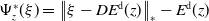 $\Psi _z^*(\xi ) = \left \|\xi - D E^{\mathrm{d}}(z)\right \|_* -E ^{\mathrm{d}}(z)$
is not fulfilled and also (2.
$\Psi _z^*(\xi ) = \left \|\xi - D E^{\mathrm{d}}(z)\right \|_* -E ^{\mathrm{d}}(z)$
is not fulfilled and also (2.
 $\Psi _3$
). In fact, a more detailed study on how these assumptions could be relaxed would be very interesting, which we, however, leave for future work.
$\Psi _3$
). In fact, a more detailed study on how these assumptions could be relaxed would be very interesting, which we, however, leave for future work.
An important special case of the above scheme is a reflexive Banach space
 $\mathcal{X}$
together with a
$\mathcal{X}$
together with a
 $C^1$
energy
$C^1$
energy
 $E$
, i.e., we can choose
$E$
, i.e., we can choose
 $E^{\mathrm{c}}=0$
. In this case, the scheme is fully explicit, as the following lemma shows.
$E^{\mathrm{c}}=0$
. In this case, the scheme is fully explicit, as the following lemma shows.
Lemma 3.12.
If the Banach space
 $\mathcal{X}$
is reflexive and
$\mathcal{X}$
is reflexive and
 $E\in C^1(\mathcal{X})$
, then we can explicitly compute the iterates in Definition
3.10
as
$E\in C^1(\mathcal{X})$
, then we can explicitly compute the iterates in Definition
3.10
as
 \begin{align*} x_{\mathrm {si},\tau }^{k+1} \in x_{\mathrm {si},\tau }^{k}-\tau \, \partial \|\cdot \|_*(D E(x_{\mathrm {si},\tau }^{k})). \end{align*}
Proof. We compute
 \begin{align*} x_{\mathrm {si},\tau }^{k+1}& \in \mathop{\mathrm{arg\,min}}\limits_{{x}\;:\; \|{x}-x_{\mathrm {si},\tau }^{k}\|\leq \tau } E(x_{\mathrm {si},\tau }^{k})+\langle D E(x_{\mathrm {si},\tau }^{k}) , {x}-x_{\mathrm {si},\tau }^{k} \rangle \\ &=\mathop{\mathrm{arg\,min}}\limits_{{x}\;:\; \|{x}-x_{\mathrm {si},\tau }^{k}\|\leq \tau } \langle D E(x_{\mathrm {si},\tau }^{k}) , {x}\rangle \\ &=-\mathop{\mathrm{arg\,max}}\limits_{{x}\;:\; \|{x}-x_{\mathrm {si},\tau }^{k}\|\leq \tau } \langle D E (x_{\mathrm {si},\tau }^{k}) , {x}\rangle \\ &=x_{\mathrm {si},\tau }^k -\tau \mathop{\mathrm{arg\,max}}\limits_{{x}\in \overline {B_1}} \langle D E(x_{\mathrm {si},\tau }^{k}), {x}\rangle \\ &=x_{\mathrm {si},\tau }^{k}-\tau \, \partial \|\cdot \|_*(D E(x_{\mathrm {si},\tau }^{k})), \end{align*}
where for the last identity, we used A.5.
In section 5, we consider a case where
 $ E^{\mathrm{c}}\neq 0$
, but the scheme can still be computed explicitly. In fact, the iteration then coincides with (IFGSM), which ultimately yields the desired convergence result.
$ E^{\mathrm{c}}\neq 0$
, but the scheme can still be computed explicitly. In fact, the iteration then coincides with (IFGSM), which ultimately yields the desired convergence result.
It is easy to see that the metric slope of
 $E$
and its semi linearization
$E$
and its semi linearization
 $E^{\mathrm{sl}}(\cdot ;z)$
coincide in the point of linearization
$E^{\mathrm{sl}}(\cdot ;z)$
coincide in the point of linearization
 $z$
, i.e.
$z$
, i.e.
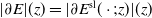 $|\partial E|(z)=|\partial E^{\mathrm{sl}}(\cdot ;z)|(z)$
. The next lemma estimates the difference of their slope when
$|\partial E|(z)=|\partial E^{\mathrm{sl}}(\cdot ;z)|(z)$
. The next lemma estimates the difference of their slope when
 $u$
is not the point of linearization.
$u$
is not the point of linearization.
Lemma 3.13.
Let
 $E$
be a
$E$
be a
 $C^1$
-perturbation of a convex function satisfying Assumption 3.a, then for each
$C^1$
-perturbation of a convex function satisfying Assumption 3.a, then for each
 $z, x\in \mathcal{X}$
, we have the following estimate
$z, x\in \mathcal{X}$
, we have the following estimate
 \begin{align} \left ||\partial E|({x})-|\partial E^{\mathrm{sl}}(\cdot ;z)|({x})\right |\leq \mathrm {Lip}(D E^{\mathrm{d}}) \|z-{x}\|. \end{align}
Proof. Let
 $z, x\in \mathcal{X}$
, from Item 1 we know
$z, x\in \mathcal{X}$
, from Item 1 we know
 \begin{align*} \partial E({x}) &= \partial E^{\mathrm{c}}({x}) + D E^{\mathrm{d}}({x}),\\ \partial E^{\mathrm{sl}}({x}; z) &= \partial E^{\mathrm{c}}({x}) + D E^{\mathrm{d}}(z), \end{align*}
and then Item 3 implies that there exists
 $\xi _1,\xi _2\in \partial E^{\mathrm{c}}({x})$
such that
$\xi _1,\xi _2\in \partial E^{\mathrm{c}}({x})$
such that
 \begin{align*} \left |\partial E\right |({x}) &= \min \left \{ \left \|\xi + D E^{\mathrm{d}}({x})\right \|_*\;:\;\xi \in \partial E^{\mathrm{c}}({x})\right \} = \left \|\xi _1 + D E^{\mathrm{d}}({x})\right \|_*,\\ \left |\partial E^{\mathrm{sl}}(\cdot ; z)\right |({x}) &= \min \left \{ \left \|\xi + D E^{\mathrm{d}}(z)\right \|_*\;:\;\xi \in \partial E^{\mathrm{c}}({x})\right \} = \left \|\xi _2 + D E^{\mathrm{d}}(z)\right \|_*. \end{align*}
We can then estimate
 \begin{align*} \left |\partial E\right |({x})&\leq \left \|D E^{\mathrm{d}}({x})+ \xi _2\right \|_* \leq \|D E^{\mathrm{d}}({x})-D E^{\mathrm{d}}(z)\|_*+\|D E^{\mathrm{d}}(z)+\xi _2\|_*\\ &\leq \mathrm {Lip}(D E^{\mathrm{d}})\|{x}-z\|+\left |\partial E^{\mathrm{sl}}(\cdot ; z)\right |({x}), \end{align*}
and therefore
 \begin{align*} \left |\partial E\right |({x}) - \left |\partial E^{\mathrm{sl}}(\cdot ;\ z)\right |({x})\leq \mathrm {Lip}(D E^{\mathrm{d}})\|{x}-z\|. \end{align*}
Analogously, we estimate
 \begin{align*} \left |\partial E^{\mathrm{sl}}(\cdot ,z)\right |({x}) &\leq \| D E^{\mathrm{d}}(z) +\xi _1\|\leq \| D E^{\mathrm{d}}(z)-D E^{\mathrm{d}}({x})\|+\|D E({x})+\xi _1\|\\ &\leq \mathrm {Lip}(D E^{\mathrm{d}})\|{x}-z\|+|\partial E| ({x}). \end{align*}
and therefore
 \begin{align*} \left |\partial E^{\mathrm{sl}}(\cdot ;\ z)\right |({x})-\left |\partial E\right |({x})\leq \mathrm {Lip}(D E^{\mathrm{d}})\|{x}-z\|. \end{align*}
This concludes the proof.
In the following, we want to define a variational interpolation similar to Definition 2.10. Therefore, we consider
 \begin{align*} E^{\mathrm{sl}}_\tau ({x};\ z) = \min _{\tilde {{x}}\in \overline {B_\tau }({x})} E^{\mathrm{sl}}(\tilde {{x}};\ z). \end{align*}
For better readability, if
 $z$
and
$z$
and
 $x$
coincide above, we set
$x$
coincide above, we set
 \begin{align*} E^{\mathrm{sl}}_\tau ({x})\;:\!=\; E^{\mathrm{sl}}_\tau ({x};\ {x})= \min _{\tilde {{x}}\in \overline {B_\tau }({x})} E^{\mathrm{sl}}(\tilde {{x}};\ {x}). \end{align*}
Definition 3.14 (Semi-implicit variational interpolation). We denote by
 $\tilde {x}_{\mathrm{si},\tau }\;:\;[0,T]\rightarrow \mathcal{X}$
any interpolation of the discrete values satisfying
$\tilde {x}_{\mathrm{si},\tau }\;:\;[0,T]\rightarrow \mathcal{X}$
any interpolation of the discrete values satisfying
 \begin{align*} \tilde {x}_{\mathrm{si},\tau }(t) \in \arg \min _{{x}} \left \{ E^{\mathrm{sl}} \big({x};\ x_{\mathrm {si},\tau }^{k-1} \big)\,:\, d \big({x},x_{\mathrm {si},\tau }^{k-1} \big)\leq t-t^{k-1}_\tau \right \} \end{align*}
if
 $t \in (t_\tau ^{k-1},t^k_\tau ]$
and
$t \in (t_\tau ^{k-1},t^k_\tau ]$
and
 $ k\geq 1$
. Furthermore, we define
$ k\geq 1$
. Furthermore, we define
 \begin{align} \mathcal{D}_\tau (t)\;:\!=\; \frac {\text{d}}{\text{d}t} E^{\mathrm{sl}}_{(t-t_\tau ^{k-1})}(x_{\mathrm {si},\tau }^{k-1}). \end{align}
The following Lemma shows that the variational interpolation of the semi-implicit minimizing movement scheme satisfies the same properties, (2.8) and (2.9), as the De Giorgi variational interpolation, up to an error in
 $\mathcal{O}(\tau )$
.
$\mathcal{O}(\tau )$
.
Lemma 3.15. We have that
 \begin{align} \mathcal{D}_\tau (t)= \frac {\text{d}}{\text{d}t} E^{\mathrm{sl}}_{ \big(t-t_\tau ^{k-1} \big)} \big(x_{\mathrm {si},\tau }^{k-1} \big) \leq -|\partial E^{\mathrm{sl}} \big(\cdot ;\ x_{\mathrm {si},\tau }^{k-1} \big)|(\tilde {x}_{\mathrm{si},\tau }(t))=-|\partial E |(\tilde {x}_{\mathrm{si},\tau }(t))+\mathcal{O}(\tau ) \text{ if } t\in (t_\tau ^{k-1},t_\tau ^k] \end{align}
and
 \begin{align} E(\tilde {x}_{\mathrm{si},\tau }(s))+\int _s^t D_\tau (r) \,\text{d}r\geq E(\tilde {x}_{\mathrm{si},\tau }(t)) +\mathcal{O}(\tau )\quad \forall \ 0\leq s\leq t\leq T. \end{align}
Proof. For (3.13), we apply Lemma 2.9 to the mapping
 ${x}\mapsto E^{\mathrm{sl}}({x};\ x_{\mathrm {si},\tau }^{k-1})$
to obtain
${x}\mapsto E^{\mathrm{sl}}({x};\ x_{\mathrm {si},\tau }^{k-1})$
to obtain
 \begin{align*} \frac {\text{d}}{\text{d}t} E^{\mathrm{sl}}_{\big(t-t_\tau ^{k-1} \big)} \big({x};\ x_{\mathrm {si},\tau }^{k-1} \big) \leq |\partial E^{\mathrm{sl}} \big(\cdot ,x_{\mathrm {si},\tau }^{k-1} \big)|\left ({x}_{\text{min},t-t^{k-1}_\tau }\right ), \end{align*}
where
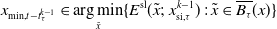 ${x}_{\mathrm{min},t-t^{k-1}_\tau }\in \displaystyle\operatorname*{arg\,min}_{\tilde {{x}}} \{E^{\mathrm{sl}}(\tilde {{x}};\ x_{\mathrm {si},\tau }^{k-1})\,:\, \tilde {{x}}\in \overline {B_\tau }({x})\}$
. Choosing
${x}_{\mathrm{min},t-t^{k-1}_\tau }\in \displaystyle\operatorname*{arg\,min}_{\tilde {{x}}} \{E^{\mathrm{sl}}(\tilde {{x}};\ x_{\mathrm {si},\tau }^{k-1})\,:\, \tilde {{x}}\in \overline {B_\tau }({x})\}$
. Choosing
 $v=x_{\mathrm {si},\tau }^{k-1}$
then yields
$v=x_{\mathrm {si},\tau }^{k-1}$
then yields
 \begin{align*} \frac {\text{d}}{\text{d}t} E^{\mathrm{sl}}_{(t-t_\tau ^{k-1})}(x_{\mathrm {si},\tau }^{k-1}) \leq -|\partial E^{\mathrm{sl}}(\cdot ;\ x_{\mathrm {si},\tau }^{k-1})|(\tilde {x}_{\mathrm{si},\tau }(t)). \end{align*}
The last equality of (3.13) follows by Lemma 3.13. To show (3.14), we again use Lemma 2.9 and get
 \begin{align*} E^{\mathrm{sl}} \big(\tilde {x}_{\mathrm{si},\tau }(s);\ x_{\mathrm {si},\tau }^k \big)+\int _{s}^t \mathcal{D}_\tau (r) \,\text{d}r\geq E^{\mathrm{sl}} \big(\tilde {x}_{\mathrm{si},\tau }(t),x_{\mathrm {si},\tau }^k \big) \quad \text{for all}\quad t_\tau ^k\leq s\leq t\leq t_\tau ^{k+1}. \end{align*}
Due to Theorem C.1
 \begin{align*} \left |E^{\mathrm{sl}}\big(\tilde {x}_{\mathrm{si},\tau }(s);\ x_{\mathrm {si},\tau }^k \big)- E(\tilde {x}_{\mathrm{si},\tau }(s))\right |&=\left | E^{\mathrm{d}} \big(x_{\mathrm {si},\tau }^k \big) + \langle D E^{\mathrm{d}}(x_{\mathrm {si},\tau }^k), \tilde {x}_{\mathrm{si},\tau }(s) - x_{\mathrm {si},\tau }^k\rangle - E^{\mathrm{d}}(\tilde {x}_{\mathrm{si},\tau }(s)) \right | \\ &\leq \bigg |\int _0^1 \left \langle D E^{\mathrm{d}}\left (x_{\mathrm {si},\tau }^k +r (\tilde {x}_{\mathrm{si},\tau }(s)-x_{\mathrm {si},\tau }^k)\right ),x_{\mathrm {si},\tau }^k -\tilde {x}_{\mathrm{si},\tau }(s) \right \rangle \\ &\quad -\langle D E^{\mathrm{d}}(x_{\mathrm {si},\tau }^k),\tilde {x}_{\mathrm{si},\tau }(t)-x_{\mathrm {si},\tau }^k \rangle \,\text{d}r\bigg |\\ &\leq \int _0^1 r \mathrm {Lip}(D E^{\mathrm{d}})\| \tilde {x}_{\mathrm{si},\tau }(s)-x_{\mathrm {si},\tau }^k\|^2\,\text{d}r \\ &\leq \frac {1}{2} \mathrm {Lip}(D E^{\mathrm{d}})\| \tilde {x}_{\mathrm{si},\tau }(s)-x_{\mathrm {si},\tau }^k\|^2 \leq \frac {1}{2} \mathrm {Lip}(D E^{\mathrm{d}}) \tau ^2 \end{align*}
and analogusly
 $|E^{\mathrm{sl}}(\tilde {x}_{\mathrm{si},\tau }(t),x_{\mathrm {si},\tau }^{k})- E(\tilde {x}_{\mathrm{si},\tau }(t))|\leq \frac {1}{2} \mathrm {Lip}(D E^{\mathrm{d}}) \tau ^2$
. Therefore, for all
$|E^{\mathrm{sl}}(\tilde {x}_{\mathrm{si},\tau }(t),x_{\mathrm {si},\tau }^{k})- E(\tilde {x}_{\mathrm{si},\tau }(t))|\leq \frac {1}{2} \mathrm {Lip}(D E^{\mathrm{d}}) \tau ^2$
. Therefore, for all
 $t_\tau ^k\leq s\leq t\leq t_\tau ^{k+1}$
, we have that
$t_\tau ^k\leq s\leq t\leq t_\tau ^{k+1}$
, we have that
 \begin{align} \begin{aligned} E(\tilde {x}_{\mathrm{si},\tau }(s))+\int _{s}^t \mathcal{D}_\tau (r) \,\text{d}r &\geq E^{\mathrm{sl}}(\tilde {x}_{\mathrm{si},\tau }(s);\ {x}_\tau ^k) +\int _{s}^t \mathcal{D}_\tau (r) \,\text{d}r -\frac {1}{2} \mathrm {Lip}(D E^{\mathrm{d}}) \tau ^2\\ &\geq E^{\mathrm{sl}}(\tilde {x}_{\mathrm{si},\tau }(t);\ {x}_\tau ^k) -\frac {1}{2} \mathrm {Lip}(D E^{\mathrm{d}}) \tau ^2\\ &\geq E(\tilde {x}_{\mathrm{si},\tau }(t)) - \mathrm {Lip}(D E^{\mathrm{d}}) \tau ^2. \end{aligned} \end{align}
Now for
 $s\in [t_\tau ^m,t_\tau ^{m+1}]$
and
$s\in [t_\tau ^m,t_\tau ^{m+1}]$
and
 $t\in [t_\tau ^k,t_\tau ^{k+1}]$
with
$t\in [t_\tau ^k,t_\tau ^{k+1}]$
with
 $m\leq k$
, we add up (3.15) to obtain
$m\leq k$
, we add up (3.15) to obtain
 \begin{align*} E(\tilde {x}_{\mathrm{si},\tau }(s))&+ \int _s^{t_\tau ^{m+1}} \mathcal{D}_\tau (r) \,\text{d}r +\sum _{i=m+1}^{k-1} \int _{t_\tau ^{i}}^{t_\tau ^{i+1}} \mathcal{D}_\tau (r) \,\text{d}r+\int _{t_\tau ^k}^t \mathcal{D}_\tau (r) \,\text{d}r \\ &\geq E(\tilde {x}_{\mathrm{si},\tau }(t))-\sum _{i=m}^k \mathrm {Lip}(D E^{\mathrm{d}}) \tau ^2\\ &=E(\tilde {x}_{\mathrm{si},\tau }(t))- (k-m) \mathrm {Lip}(D E^{\mathrm{d}}) \tau ^2\\ &\geq E(\tilde {x}_{\mathrm{si},\tau }(t))- T \mathrm {Lip}(D E^{\mathrm{d}}) \tau \end{align*}
such that we finally obtain (3.14).
As an immediate consequence of Lemma 3.15, we can replace the minimizing movement scheme in the proof of Theorem 2.11 by the semi-implicit scheme, as the error terms are of order
 $\mathcal{O}(\tau )$
and vanish during the limiting process
$\mathcal{O}(\tau )$
and vanish during the limiting process
 $\tau \rightarrow 0$
. Then
$\tau \rightarrow 0$
. Then
 $\bar {x}_{\mathrm{si},\tau }$
 $\sigma$
-converges up to a subsequence to a
$\sigma$
-converges up to a subsequence to a
 $\infty$
-curve of maximal slope.
$\infty$
-curve of maximal slope.
Theorem 3.16.
Let
 $E$
be a
$E$
be a
 $C^1$
-perturbation of a convex function. Under Assumptions 1.a to 3.b, there exists a
$C^1$
-perturbation of a convex function. Under Assumptions 1.a to 3.b, there exists a
 $\infty$
-curve of maximal slope
$\infty$
-curve of maximal slope
 $u(t)$
, with respect to the energy
$u(t)$
, with respect to the energy
 $ E$
and its upper gradient
$ E$
and its upper gradient
 $|\partial E|$
, and a subsequence of
$|\partial E|$
, and a subsequence of
 $\tau _n=T/n$
such that
$\tau _n=T/n$
such that
 \begin{align*} \bar {x}_{\mathrm{si},\tau _n}(t) \stackrel {\sigma }{\rightharpoonup }u(t) \text{ as } n\rightarrow \infty \quad \forall t\in [0,T]. \end{align*}
Proof. We simply replace the minimizing movement scheme in Definition 2.5 and De Giorgis variational interpolation (see Definition 2.10) by the semi-implicit scheme in Definition 3.10 and its corresponding variational interpolation of Lemma 3.15. Proceeding similarly as in the proof of Theorem 2.11, we use Proposition B.1 to show
 \begin{align*} \bar {x}_{\mathrm{si},\tau _n}(t) \stackrel {\sigma }{\rightharpoonup }u(t) \text{ as } n\rightarrow \infty \quad \forall t\in [0,T] \end{align*}
for a subsequence
 $\tau _n$
, where
$\tau _n$
, where
 $u$
is a
$u$
is a
 $1$
-Lipschitz curve with
$1$
-Lipschitz curve with
 $u(0)={x}^0$
. Then the same holds true for
$u(0)={x}^0$
. Then the same holds true for
 $\tilde {x}_{\mathrm{si},\tau _n}(t)$
.
$\tilde {x}_{\mathrm{si},\tau _n}(t)$
.
Taking for
 $\tau _n$
the limes inferior for
$\tau _n$
the limes inferior for
 $n\rightarrow \infty$
of (3.14) and using Assumption 2.a, Assumption 2.b and (3.13) we again obtain
$n\rightarrow \infty$
of (3.14) and using Assumption 2.a, Assumption 2.b and (3.13) we again obtain
 \begin{align*} E(u(0))\geq E(u(t))+\int _0^t |\partial E|(u(r)) \,\text{d}r \quad \text{ for all }t\in [0,T]. \end{align*}
Since on the other hand
 $|\partial E|$
is a strong upper gradient, equality in the above equation must hold.
$|\partial E|$
is a strong upper gradient, equality in the above equation must hold.
Remark 3.17. Let
 $\tau _n$
be any sequence such that
$\tau _n$
be any sequence such that
 $\tau _n \rightarrow 0$
. If the
$\tau _n \rightarrow 0$
. If the
 $\infty$
-curve of maximal slope
$\infty$
-curve of maximal slope
 $u$
is unique, we can apply Theorem 3.16 to every subsequence of
$u$
is unique, we can apply Theorem 3.16 to every subsequence of
 $\tau _n$
and find a further subsequence
$\tau _n$
and find a further subsequence
 $\tilde {\tau }_n$
such that
$\tilde {\tau }_n$
such that
 \begin{align*} \bar {x}_{\mathrm{si},\tilde {\tau }_n}(t) \stackrel {\sigma }{\rightharpoonup }u(t) \text{ as } n\rightarrow \infty \quad \forall t\in [0,T]. \end{align*}
This implies that already for
 $\tau _n$
 \begin{align*} \bar {x}_{\mathrm{si},\tau _n}(t) \stackrel {\sigma }{\rightharpoonup }u(t) \text{ as } n\rightarrow \infty \quad \forall t\in [0,T]. \end{align*}
and the semi-implicit scheme converges.
4. Wasserstein infinity flows
The previous sections consider a “single particle”,
 ${x}\in \mathcal{X}$
, trying to minimize an energy
${x}\in \mathcal{X}$
, trying to minimize an energy
 $\mathcal{E}$
, by following an
$\mathcal{E}$
, by following an
 $\infty$
-curve of maximal slope. This single particle may be drawn from a probability distribution
$\infty$
-curve of maximal slope. This single particle may be drawn from a probability distribution
 $\mu _0 \in \mathcal{P}(\mathcal{X})$
, which over time also minimizes an energy
$\mu _0 \in \mathcal{P}(\mathcal{X})$
, which over time also minimizes an energy
 $\mathcal{E}$
defined on the space of probabilities. In this section, we choose the underlying metric space
$\mathcal{E}$
defined on the space of probabilities. In this section, we choose the underlying metric space
 $\mathcal{S}$
to be the space of Borel probability measures with bounded support
$\mathcal{S}$
to be the space of Borel probability measures with bounded support
 $\mathcal{P}_\infty (\mathcal{X})$
, and equip it with the
$\mathcal{P}_\infty (\mathcal{X})$
, and equip it with the
 $\infty$
-Wasserstein distance. We show that for potential energies,
$\infty$
-Wasserstein distance. We show that for potential energies,
 $\infty$
-curves of maximal slope can be expressed via a probability measures
$\infty$
-curves of maximal slope can be expressed via a probability measures
 $\eta$
on the space
$\eta$
on the space
 $C(0,T;\;\mathcal{X})$
, which is concentrated on
$C(0,T;\;\mathcal{X})$
, which is concentrated on
 $\infty$
-curves of maximal slope on the underlying Banach space
$\infty$
-curves of maximal slope on the underlying Banach space
 $\mathcal{X}$
. From
$\mathcal{X}$
. From
 $\eta$
, we can then derive a corresponding continuity equation which those
$\eta$
, we can then derive a corresponding continuity equation which those
 $\infty$
-curves of maximal slope have to fulfil.
$\infty$
-curves of maximal slope have to fulfil.
This concept is commonly referred to as the “superposition principle”, where our approach directly follows the setup of [Reference Ambrosio, Gigli and Savaré2, Reference Lisini62, Reference Lisini63]. We refer to [Reference Stepanov and Trevisan99] for an overview of different works in this direction, as well as results that hold true in a much more general setting.
4.1. Preliminaries on Wasserstein spaces
We give a brief introduction to the basic properties of Wasserstein spaces. For more details, we refer to [Reference Ambrosio, Gigli and Savaré2, Reference Givens and Shortt44, Reference Villani104]. In the following,
 $(\mathcal{X}, \|\cdot \|)$
is a separable Banach space. We denote by
$(\mathcal{X}, \|\cdot \|)$
is a separable Banach space. We denote by
 $\mathcal{P}(\mathcal{X})$
the space of Borel probability measures on
$\mathcal{P}(\mathcal{X})$
the space of Borel probability measures on
 $\mathcal{X}$
. For
$\mathcal{X}$
. For
 $1\leq p\lt \infty$
,
$1\leq p\lt \infty$
,
 $\mathcal{P}_p(\mathcal{X}) \subset \mathcal{P}(\mathcal{X})$
is the subset of measures with finite
$\mathcal{P}_p(\mathcal{X}) \subset \mathcal{P}(\mathcal{X})$
is the subset of measures with finite
 $p$
-momentum, while
$p$
-momentum, while
 $\mathcal{P}_\infty (\mathcal{X})\subset \mathcal{P}(\mathcal{X})$
is the subset of measures with bounded support. For
$\mathcal{P}_\infty (\mathcal{X})\subset \mathcal{P}(\mathcal{X})$
is the subset of measures with bounded support. For
 $1\leq p\lt \infty$
and
$1\leq p\lt \infty$
and
 $\mu ,\nu \in \mathcal{P}_p(\mathcal{X})$
, we define the
$\mu ,\nu \in \mathcal{P}_p(\mathcal{X})$
, we define the
 $p$
-Wasserstein distance as
$p$
-Wasserstein distance as
 \begin{align*} W^p_p(\mu ,\nu )\;:\!=\; \inf _{\gamma \in \Gamma (\mu ,\nu )} \int \| {x}-z\|^p \text{d}\gamma ({x},z). \end{align*}
Here,
 \begin{align} \Gamma (\mu ,\nu )\;:\!=\;\{\gamma \in \mathcal{P}(\mathcal{X}\times \mathcal{X}): \pi ^1_\# \gamma =\mu , \pi ^2_\# \gamma =\nu \}, \end{align}
is the set of admissible transport plans and
 $\pi ^1({x},z)={x}$
,
$\pi ^1({x},z)={x}$
,
 $\pi ^2({x},z)=z$
denote the projection on the first and second component. For
$\pi ^2({x},z)=z$
denote the projection on the first and second component. For
 $\mu ,\nu \in \mathcal{P}_\infty (\mathcal{X})$
, the
$\mu ,\nu \in \mathcal{P}_\infty (\mathcal{X})$
, the
 $\infty$
-Wasserstein distance is given by
$\infty$
-Wasserstein distance is given by
 \begin{align} W_\infty (\mu ,\nu )\;:\!=\; \inf _{\gamma \in \Gamma (\mu ,\nu )} \gamma -\operatorname{ess\,sup} \| {x}-z\|. \end{align}
In both cases, the minimum of (4.1) and (4.2) is obtained (see, e.g., [Reference Ambrosio, Gigli and Savaré2, Reference Villani104] and [Reference Givens and Shortt44, Proposition 1] for the case
 $p=\infty$
) and
$p=\infty$
) and
 $\Gamma _0(\mu ,\nu )$
denotes the set of optimal transport plans where the minimum is reached.
$\Gamma _0(\mu ,\nu )$
denotes the set of optimal transport plans where the minimum is reached.
Proposition 4.1 [Reference Givens and Shortt44, Proposition 6.]. For
 $p\in [1,\infty ]$
,
$p\in [1,\infty ]$
,
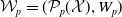 $\mathcal{W}_p=(\mathcal{P}_p(\mathcal{X}), W_p)$
, i.e.,
$\mathcal{W}_p=(\mathcal{P}_p(\mathcal{X}), W_p)$
, i.e.,
 $\mathcal{P}_p(\mathcal{X})$
equipped with the
$\mathcal{P}_p(\mathcal{X})$
equipped with the
 $p$
-Wasserstein distance, is a complete metric space. For
$p$
-Wasserstein distance, is a complete metric space. For
 $p\lt \infty$
,
$p\lt \infty$
,
 $\mathcal{W}_p$
is separable.
$\mathcal{W}_p$
is separable.
The following lemma shows that Wasserstein distances are ordered in such a way that they get stronger by increasing
 $p$
, see [Reference Givens and Shortt44, Proposition 3.].
$p$
, see [Reference Givens and Shortt44, Proposition 3.].
Lemma 4.2 [Reference Givens and Shortt44, Proposition 3.]. For
 $1\leq p\leq q \leq \infty$
and
$1\leq p\leq q \leq \infty$
and
 $\mu ,\nu \in \mathcal{P}(\mathcal{X})$
 \begin{align} W_p(\mu ,\nu )\leq W_q(\mu ,\nu ) \end{align}
and in particular
 \begin{align*} W_\infty (\mu ,\nu )=\sup _p W_p(\mu ,\nu )=\lim _{p\rightarrow \infty }W_p(\mu ,\nu ). \end{align*}
Let now
 $\sigma$
denote the narrow topology, namely,
$\sigma$
denote the narrow topology, namely,
 $\mu ^n\stackrel {\sigma }{\rightarrow } \mu$
iff,
$\mu ^n\stackrel {\sigma }{\rightarrow } \mu$
iff,
 \begin{align} \int _{\mathcal{X}} \varphi \,\text{d}\mu ^n \rightarrow \int _{\mathcal{X}} \varphi \,\text{d}\mu \quad \forall \varphi \in C_b(\mathcal{X}), \end{align}
where
 $C_b(\mathcal{X})$
denotes the space of bounded and continuous functions on
$C_b(\mathcal{X})$
denotes the space of bounded and continuous functions on
 $\mathcal{X}$
. The next lemma is helpful, when we are considering limits in (4.4) with
$\mathcal{X}$
. The next lemma is helpful, when we are considering limits in (4.4) with
 $\varphi$
being unbounded or only lower semicontinuous.
$\varphi$
being unbounded or only lower semicontinuous.
Lemma 4.3 [Reference Ambrosio, Gigli and Savaré2, Lemma 5.1.7.]. Let
 $\left (\mu ^{n}\right )_{n\in \mathbb{N}}$
be a sequence in
$\left (\mu ^{n}\right )_{n\in \mathbb{N}}$
be a sequence in
 $\mathcal{P}(\mathcal{X})$
narrowly converging to
$\mathcal{P}(\mathcal{X})$
narrowly converging to
 $\mu \in \mathcal{P}(\mathcal{X})$
. If
$\mu \in \mathcal{P}(\mathcal{X})$
. If
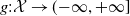 $g: \mathcal{X} \rightarrow ({-}\infty ,+\infty ]$
is lower semicontinuous and its negative part
$g: \mathcal{X} \rightarrow ({-}\infty ,+\infty ]$
is lower semicontinuous and its negative part
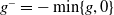 $g^-=-\min \{g,0\}$
is uniformly integrable w.r.t. the set
$g^-=-\min \{g,0\}$
is uniformly integrable w.r.t. the set
 $\{\mu ^n\}_{n\in \mathbb{N}}$
, then
$\{\mu ^n\}_{n\in \mathbb{N}}$
, then
 \begin{align*} \liminf _{n\rightarrow \infty }\int _{\mathcal{X}} g(x)d \mu ^n(x)\geq \int _{\mathcal{X}} g(x) \,\text{d}\mu (x) \gt -\infty . \end{align*}
When working with probability measures, Prokhorov’s theorem ([Reference Billingsley7, Theorems 5.1–5.2], repeated for convenience in the appendix, Theorem D.1) is useful since it characterizes relatively compact sets with respect to the narrow topology. In certain situations, the assumption (D.1) of this theorem, i.e.,
 \begin{align*} \forall \epsilon \gt 0\quad \exists K_\epsilon \text{ compact in } \mathcal{X} \text{ such that } \mu (\mathcal{X}\setminus K_\epsilon )\leq \epsilon \quad \forall \mu \in \mathcal{K}, \end{align*}
can only be shown for bounded and not compact sets. There, we use the observation in the following remark to still obtain some sort of relative compactness. In the following, we denote by
 $\mathcal{X}_\omega$
, the space
$\mathcal{X}_\omega$
, the space
 $\mathcal{X}$
equipped with the weak topology
$\mathcal{X}$
equipped with the weak topology
 $\sigma (\mathcal{X},\mathcal{X}^*)$
.
$\sigma (\mathcal{X},\mathcal{X}^*)$
.
Remark 4.4. If
 $\mathcal{X}$
is separable and reflexive, then so is its dual. For a countable dense subset
$\mathcal{X}$
is separable and reflexive, then so is its dual. For a countable dense subset
 $\{x^*_n\}_{n\in \mathbb{N}}$
of
$\{x^*_n\}_{n\in \mathbb{N}}$
of
 $\overline {B_1^{\mathcal{X}*}}$
, we can define the norm
$\overline {B_1^{\mathcal{X}*}}$
, we can define the norm
 \begin{equation*}\| x \|_{\omega }=\sum _{n=1}^\infty \frac {1}{n^2} |\langle x^*_n,x\rangle |,\end{equation*}
which induces the weak topology
 $\sigma (\mathcal{X},\mathcal{X}^*)$
on bounded sets [Reference Morrison73, Lemma 3.2]. This norm is a so-called Kadec norm. In particular, we have that the Borel sigma algebra
$\sigma (\mathcal{X},\mathcal{X}^*)$
on bounded sets [Reference Morrison73, Lemma 3.2]. This norm is a so-called Kadec norm. In particular, we have that the Borel sigma algebra
 $\mathcal{B}(\mathcal{X})$
, generated by the norm topology, and the one generated by the weak topology
$\mathcal{B}(\mathcal{X})$
, generated by the norm topology, and the one generated by the weak topology
 $\mathcal{B}(\mathcal{X}_{\omega })$
coincide and thus
$\mathcal{B}(\mathcal{X}_{\omega })$
coincide and thus
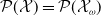 $\mathcal{P}(\mathcal{X})=\mathcal{P}(\mathcal{X}_\omega )$
, see [Reference Edgar37, Theorem 1.1]. Now, let us assume that for a set
$\mathcal{P}(\mathcal{X})=\mathcal{P}(\mathcal{X}_\omega )$
, see [Reference Edgar37, Theorem 1.1]. Now, let us assume that for a set
 $\mathcal{K}\subset \mathcal{P}(\mathcal{X})=\mathcal{P}(\mathcal{X}_\omega )$
, we have that
$\mathcal{K}\subset \mathcal{P}(\mathcal{X})=\mathcal{P}(\mathcal{X}_\omega )$
, we have that
 \begin{align} \forall \epsilon \gt 0\quad \exists K_\epsilon \ \|\cdot \|\text{-bounded in } \mathcal{X}, \text{ such that } \mu (\mathcal{X}\setminus K_\epsilon )\leq \epsilon \quad \forall \mu \in \mathcal{K}. \end{align}
Since bounded sets are subsets of
 $\overline {B_\epsilon }$
for
$\overline {B_\epsilon }$
for
 $\epsilon$
large enough and
$\epsilon$
large enough and
 $\overline {B_\epsilon }$
is compact in the weak topology
$\overline {B_\epsilon }$
is compact in the weak topology
 $\sigma (\mathcal{X},\mathcal{X}^*)$
, Prokhorov’s theorem can be applied for
$\sigma (\mathcal{X},\mathcal{X}^*)$
, Prokhorov’s theorem can be applied for
 $\mathcal{X}_\omega$
. We obtain that there exists a subsequence
$\mathcal{X}_\omega$
. We obtain that there exists a subsequence
 $\left (\mu ^{n}\right )_{n\in \mathbb{N}}\subset \mathcal{K}$
and a limit
$\left (\mu ^{n}\right )_{n\in \mathbb{N}}\subset \mathcal{K}$
and a limit
 $\mu \in \mathcal{P}(\mathcal{X})=\mathcal{P}(\mathcal{X}_\omega )$
such that
$\mu \in \mathcal{P}(\mathcal{X})=\mathcal{P}(\mathcal{X}_\omega )$
such that
 \begin{align} \int _{\mathcal{X}} \varphi \,\text{d}\mu ^n \rightarrow \int _{\mathcal{X}} \varphi \,\text{d}\mu \quad \forall \varphi \in C^\omega _b(\mathcal{X}), \end{align}
where
 $C^\omega _b(\mathcal{X})$
now denotes the set of weakly continuous bounded functions.
$C^\omega _b(\mathcal{X})$
now denotes the set of weakly continuous bounded functions.
The next lemma follows from [Reference Villani104, Theorem 6.9, Corollary 6.11, Remark 6.12] together Lemma 4.2, i.e., [Reference Givens and Shortt44, Proposition 3].
Lemma 4.5 (Compatibility). The narrow topology
 $\sigma$
is weaker than the topology induced by
$\sigma$
is weaker than the topology induced by
 $W_p(\cdot ,\cdot )$
on
$W_p(\cdot ,\cdot )$
on
 $\mathcal{P}_p(\mathcal{X})$
, for every
$\mathcal{P}_p(\mathcal{X})$
, for every
 $p\in [1,\infty ]$
. Furthermore,
$p\in [1,\infty ]$
. Furthermore,
 $W_p$
is lower semicontinuous with respect to the narrow topology
$W_p$
is lower semicontinuous with respect to the narrow topology
 $\sigma$
, i.e., for every
$\sigma$
, i.e., for every
 $p\in [1,\infty ]$
:
$p\in [1,\infty ]$
:
 \begin{align*} \left . \begin{array}{ll} \mu ^n\stackrel {\sigma }{\rightarrow } \mu \\ \nu ^n\stackrel {\sigma }{\rightarrow } \nu \end{array} \right \} \Longrightarrow W_p(\mu ,\nu )\leq \liminf _{n\rightarrow \infty }W_p(\mu ^n,\nu ^n). \end{align*}
Remark 4.6. For
 $1\leq p\lt \infty$
, convergence in
$1\leq p\lt \infty$
, convergence in
 $W_p$
is equivalent to narrow convergence and convergence of the
$W_p$
is equivalent to narrow convergence and convergence of the
 $p$
-th moment [Reference Villani104, Theorem 6.9]. This equality is lost for the
$p$
-th moment [Reference Villani104, Theorem 6.9]. This equality is lost for the
 $\infty$
-Wasserstein distance, as convergence in the narrow topology (
$\infty$
-Wasserstein distance, as convergence in the narrow topology (
 $\mu ^n\stackrel {\sigma }{\rightarrow } \mu$
) together with
$\mu ^n\stackrel {\sigma }{\rightarrow } \mu$
) together with
 $\displaystyle\bigcup _n \operatorname{supp}(\mu ^n)$
being bounded or relatively compact no longer guarantees convergence in
$\displaystyle\bigcup _n \operatorname{supp}(\mu ^n)$
being bounded or relatively compact no longer guarantees convergence in
 $W_\infty$
, as Example 3 demonstrates.
$W_\infty$
, as Example 3 demonstrates.
Example 3. We consider the sequence
 \begin{equation*}\mu ^n=\frac {n-1}{n}\, \delta _0+\frac {1}{n}\, \delta _1,\end{equation*}
where
 $\delta _t$
denotes the Dirac measure at
$\delta _t$
denotes the Dirac measure at
 $t\in {\mathbb{R}}$
. Then we have that
$t\in {\mathbb{R}}$
. Then we have that
 \begin{align*} \int _{\mathbb{R}} \varphi \,\text{d}\mu ^n = \frac {n-1}{n}\, \varphi (0)+\frac {1}{n}\, \varphi (1) \xrightarrow []{n\to \infty } \varphi (0) = \int _{\mathbb{R}} \varphi d\delta _0 \end{align*}
for every
 $\varphi \in C_b({\mathbb{R}})$
and thus
$\varphi \in C_b({\mathbb{R}})$
and thus
 $\mu ^n\stackrel {\sigma }{\rightarrow } \delta _0$
. However, we see that
$\mu ^n\stackrel {\sigma }{\rightarrow } \delta _0$
. However, we see that
 \begin{align*} W_\infty (\mu ^n,\delta _0) = \min _{\gamma \in \Gamma (\mu ^n,\delta _0)} \gamma -\operatorname{ess\,sup} \left |{x}-z\right | = \left |1 - 0\right | = 1, \end{align*}
for every
 $n\in \mathbb{N}$
and thus we have no convergence in
$n\in \mathbb{N}$
and thus we have no convergence in
 $W_\infty$
.
$W_\infty$
.
4.2. Absolutely continuous curves in Wasserstein spaces and the superposition principle
In this section, we employ the superposition principle to obtain alternative characterizations of absolutely continuous curves in Wasserstein spaces.
In [Reference Lisini62], Lisini shows that for
 $p\in (1,\infty )$
,
$p\in (1,\infty )$
,
 $p$
-absolutely continuous curves
$p$
-absolutely continuous curves
 $\mu \;:\;[0,T]\to W_p$
can be written as a push forward of a Borel probability measure over the space of continuous curves. Using this statement, the author was able to derive a well-known characterization of absolutely continuous curves via solutions of continuity equations, when the underlying space of
$\mu \;:\;[0,T]\to W_p$
can be written as a push forward of a Borel probability measure over the space of continuous curves. Using this statement, the author was able to derive a well-known characterization of absolutely continuous curves via solutions of continuity equations, when the underlying space of
 $W_p$
is Banach. In [Reference Lisini63], the first result was extended to Wasserstein–Orlicz spaces, which also covers the
$W_p$
is Banach. In [Reference Lisini63], the first result was extended to Wasserstein–Orlicz spaces, which also covers the
 $W_\infty$
case.
$W_\infty$
case.
In [Reference Stepanov and Trevisan99, Section 4], the authors were able to derive a refined version of the result obtained in [Reference Lisini62] that also includes the case
 $p=\infty$
. For completeness, we state the corresponding theorems in this section and provide the proofs that specifically adapt the arguments of [Reference Lisini62] to our setting in Appendix E.
$p=\infty$
. For completeness, we state the corresponding theorems in this section and provide the proofs that specifically adapt the arguments of [Reference Lisini62] to our setting in Appendix E.
Connected to this, we also refer to the discussion in the book by [Reference Santambrogio91, Ch. 5.5.1] and the associated paper [Reference Brasco and Santambrogio10], where this topic was discussed as the limit
 $p\to \infty$
, for
$p\to \infty$
, for
 $\mathcal{X}={\mathbb{R}}^d$
. We further discuss difficulties arising when the norm of underlying Banach space is not strictly convex.
$\mathcal{X}={\mathbb{R}}^d$
. We further discuss difficulties arising when the norm of underlying Banach space is not strictly convex.
Let
 $\mathcal{P}(C(0,T;\;\mathcal{X}))$
denote the space of Borel probability measures on the Banach space of continuous functions on the interval
$\mathcal{P}(C(0,T;\;\mathcal{X}))$
denote the space of Borel probability measures on the Banach space of continuous functions on the interval
 $[0,T]$
. We define the evaluation map
$[0,T]$
. We define the evaluation map
 $e_t: C(0,T;\;\mathcal{X})\rightarrow \mathcal{X}$
by
$e_t: C(0,T;\;\mathcal{X})\rightarrow \mathcal{X}$
by
 \begin{equation*} e_t(u)=u(t).\end{equation*}
Then absolutely continuous curves in Wasserstein spaces can be represented by a Borel probability measure on
 $C(0,T;\;\mathcal{X})$
concentrated on the set of absolutely continuous curves in
$C(0,T;\;\mathcal{X})$
concentrated on the set of absolutely continuous curves in
 $\mathcal{X}$
, as the following theorem from [Reference Lisini63] shows. Here,
$\mathcal{X}$
, as the following theorem from [Reference Lisini63] shows. Here,
 ${\mathrm{AC}}^p(0,T ; W_p)$
denotes the set of
${\mathrm{AC}}^p(0,T ; W_p)$
denotes the set of
 $p$
-absolutely continuous curves
$p$
-absolutely continuous curves
 $\mu \;:\;[0,T]\to W_p$
.
$\mu \;:\;[0,T]\to W_p$
.
Theorem 4.7 [Reference Lisini63, Theorem 3.1]. Let
 $\mathcal{X}$
be separable. For
$\mathcal{X}$
be separable. For
 $p\in (1,\infty ]$
, if
$p\in (1,\infty ]$
, if
 $\mu \in {\mathrm{AC}}^p(0,T; \mathcal{W} _p)$
, then there exists
$\mu \in {\mathrm{AC}}^p(0,T; \mathcal{W} _p)$
, then there exists
 $\eta \in \mathcal{P}(C(0,T;\;\mathcal{X}))$
such that
$\eta \in \mathcal{P}(C(0,T;\;\mathcal{X}))$
such that
-
•
$\eta$
is concentrated on
${\mathrm{AC}}^p(0,T;\;\mathcal{X})$
, -
•
${e_t}_\# \eta =\mu _t\quad \forall t\in [0,T]$
, -
• for a.e.
$t\in [0,T]$
the metric derivative
$|u'|(t)$
exists for
$\eta$
-a.e.
$u\in C(0,T;\;\mathcal{X})$
and it holds the equality
\begin{equation*} |\mu '|(t)=\| |u'|(t)\|_{L_p(\eta )}.\end{equation*}


For a Banach space
 $(\mathcal{X},\|\cdot \|)$
and a finite measure space
$(\mathcal{X},\|\cdot \|)$
and a finite measure space
 $(\Omega , \mathcal{A},\mu )$
, we denote for
$(\Omega , \mathcal{A},\mu )$
, we denote for
 $1\leq p\leq \infty$
the Lebesgue–Bochner space by
$1\leq p\leq \infty$
the Lebesgue–Bochner space by
 $L^p(\mu ;\mathcal{X})$
. A function
$L^p(\mu ;\mathcal{X})$
. A function
 $f: \Omega \rightarrow \mathcal{X}$
belongs to
$f: \Omega \rightarrow \mathcal{X}$
belongs to
 $L^p(\mu ;\mathcal{X})$
if it is
$L^p(\mu ;\mathcal{X})$
if it is
 $\mu$
-Bochner integrable and its norm
$\mu$
-Bochner integrable and its norm
 \begin{align*} \|f\|_{L_p(\mu ;\mathcal{X})}^p&\;:\!=\; \int _{\Omega } \|f\|^p \,\text{d}\mu \quad \text{for}\quad 1\leq p \lt \infty ,\\ \|f\|_{L_\infty (\mu ;\mathcal{X})}&\;:\!=\;\mu -\operatorname{ess\,sup} \|f\|\quad p =\infty , \end{align*}
is finite, see [Reference Diestel and Uhl34]. For a narrowly continuous curve
 $\mu : [0,T]\rightarrow \mathcal{P}_p(\mathcal{X})$
, we define
$\mu : [0,T]\rightarrow \mathcal{P}_p(\mathcal{X})$
, we define
 $\bar {\mu }\in \mathcal{P}([0,T]\times \mathcal{X})$
by
$\bar {\mu }\in \mathcal{P}([0,T]\times \mathcal{X})$
by
 \begin{align*} \int _{[0,T]\times \mathcal{X} } \varphi (t,x) d\bar {\mu }\;:\!=\; \frac {1}{T}\int _{[0,T]} \int _{\mathcal{X}} \varphi (t,x) \,\text{d}\mu _t (x) \,\text{d}t \end{align*}
for every bounded Borel function
 $\varphi : [0,T]\times \mathcal{X}\rightarrow {\mathbb{R}}$
. Let
$\varphi : [0,T]\times \mathcal{X}\rightarrow {\mathbb{R}}$
. Let
 $\boldsymbol{v}\;:\;[0,T]\times \mathcal{X} \rightarrow \mathcal{X}$
be a time dependent velocity field belonging to
$\boldsymbol{v}\;:\;[0,T]\times \mathcal{X} \rightarrow \mathcal{X}$
be a time dependent velocity field belonging to
 $L^p(\bar {\mu },\mathcal{X})$
, then we say
$L^p(\bar {\mu },\mathcal{X})$
, then we say
 $(\mu ,\boldsymbol{v})$
satisfies the continuity equation
$(\mu ,\boldsymbol{v})$
satisfies the continuity equation
 \begin{align} \partial \mu _t +{\mathrm{div}}( \boldsymbol{v} _t \mu _t)=0, \end{align}
if the relation
 \begin{align*} \frac {\text{d}}{\text{d}t} \int _{\mathcal{X}} \varphi \,\text{d}\mu _t =\int _{\mathcal{X}}\langle D\varphi , \boldsymbol{v} _t\rangle \,\text{d}\mu _t \quad \forall \varphi \in C^1_b(\mathcal{X}) \end{align*}
holds in the sense of distributions in
 $(0,T)$
. Here,
$(0,T)$
. Here,
 $C^1_b(\mathcal{X})$
denotes the space of bounded, Fréchet-differentiable functions
$C^1_b(\mathcal{X})$
denotes the space of bounded, Fréchet-differentiable functions
 $\varphi \;:\;\mathcal{X}\rightarrow \mathbb{R}$
, such that
$\varphi \;:\;\mathcal{X}\rightarrow \mathbb{R}$
, such that
 $D\varphi \;:\;\mathcal{X}\rightarrow \mathcal{X}^*$
is continuous and bounded. Using this notion, we define,
$D\varphi \;:\;\mathcal{X}\rightarrow \mathcal{X}^*$
is continuous and bounded. Using this notion, we define,
 \begin{align*} \mathrm{EC}^p(\mathcal{X})\;:\!=\; \left \{ (\mu ,\boldsymbol{v})\,:\, \begin{aligned} \mu \;:\;[0,T] \rightarrow \mathcal{P}_p(\mathcal{X}) \quad &\text{is narrowly continous}, \boldsymbol{v}\in L^p(\bar {\mu };\mathcal{X}),\\(\mu ,\boldsymbol{v})\quad &\text{satisfies the continuity equation} \end{aligned}\right \}. \end{align*}
As the next theorem shows, the curves contained in the support of
 $\eta$
in Theorem 4.7 can be understood as the “characteristics” of a corresponding transport equation. The statement is an extension of [Reference Lisini62, Theorem 7] to the case
$\eta$
in Theorem 4.7 can be understood as the “characteristics” of a corresponding transport equation. The statement is an extension of [Reference Lisini62, Theorem 7] to the case
 $p=\infty$
. For completeness, we give an adapted proof in Appendix E. Here we assume that the Banach space also has the Radon–Nikodým property, see, e.g., [Reference Ryan89, Ch. 5], which we recall in the following. In particular, every reflexive Banach space has this property, see [Reference Ryan89, Corollary 5.45].
$p=\infty$
. For completeness, we give an adapted proof in Appendix E. Here we assume that the Banach space also has the Radon–Nikodým property, see, e.g., [Reference Ryan89, Ch. 5], which we recall in the following. In particular, every reflexive Banach space has this property, see [Reference Ryan89, Corollary 5.45].
Definition 4.8 (Radon–Nikodým property). We say that a Banach space
 $\mathcal{X}$
has the Radon–Nikodým property, if for every vector measure
$\mathcal{X}$
has the Radon–Nikodým property, if for every vector measure
 $\mu$
of bounded variation defined over a
$\mu$
of bounded variation defined over a
 $\sigma$
-algebra
$\sigma$
-algebra
 $\Sigma$
over
$\Sigma$
over
 $\mathcal{X}$
, that is absolutely continuous with respect to a finite, positive measure
$\mathcal{X}$
, that is absolutely continuous with respect to a finite, positive measure
 $\lambda$
, there exists a
$\lambda$
, there exists a
 $\lambda$
-Bochner integrable function
$\lambda$
-Bochner integrable function
 $f$
such that
$f$
such that
 $\mu (A) = \int _A f \,\text{d}\lambda$
for all
$\mu (A) = \int _A f \,\text{d}\lambda$
for all
 $A\in \Sigma$
.
$A\in \Sigma$
.
Theorem 4.9.
Let
 $\mathcal{X}$
be separable and satisfy the Radon–Nikodým property. If
$\mathcal{X}$
be separable and satisfy the Radon–Nikodým property. If
 $\mu \in {\mathrm{AC}}^\infty ([0,T];\mathcal{W}_\infty )$
, then there exists a vector field
$\mu \in {\mathrm{AC}}^\infty ([0,T];\mathcal{W}_\infty )$
, then there exists a vector field
 $\boldsymbol{v}\;:\; [0,T]\times \mathcal{X}\rightarrow \mathcal{X}$
such that
$\boldsymbol{v}\;:\; [0,T]\times \mathcal{X}\rightarrow \mathcal{X}$
such that
 $(\mu ,\boldsymbol{v})\in \mathrm{EC}^\infty (\mathcal{X})$
and
$(\mu ,\boldsymbol{v})\in \mathrm{EC}^\infty (\mathcal{X})$
and
 \begin{gather} \| \boldsymbol{v} _t\|_{L^ \infty (\mu _t;\mathcal{X})}\leq |\mu '|(t) \quad \text{for a.e. } t\in (0,T). \end{gather}
If in addition
 $\mathcal{X}$
satisfies the bounded approximation property (BAP), then the following Theorem 4.11 acts as the counterpart of Theorem 4.9 and states that solutions of the continuity equation are absolutely continuous curves. In particular, for a specific
$\mathcal{X}$
satisfies the bounded approximation property (BAP), then the following Theorem 4.11 acts as the counterpart of Theorem 4.9 and states that solutions of the continuity equation are absolutely continuous curves. In particular, for a specific
 $\mu \in {\mathrm{AC}}^p([0,T];\mathcal{W}_p)$
, the velocity
$\mu \in {\mathrm{AC}}^p([0,T];\mathcal{W}_p)$
, the velocity
 $\boldsymbol{v}$
field obtained in Theorem 4.9 is minimal in the sense that
$\boldsymbol{v}$
field obtained in Theorem 4.9 is minimal in the sense that
 \begin{align*} \|\boldsymbol{v}_t\|_{L^p(\mu ;\mathcal{X})} =|\mu '|(t)\leq \|\tilde {\boldsymbol{v}}_t\|_{L^p(\mu ;\mathcal{X})}\quad \text{for a.e.} \ t\in (0,T)\text{ and for all } \tilde {\boldsymbol{v}}\text{ satisfying } (\mu ,\tilde {\boldsymbol{v}})\in \mathrm{EC}^p(\mathcal{X}). \end{align*}
We briefly recall the (BAP) and then state Theorem 4.11, which is an extension of [Reference Lisini62, Theorem 8] to
 $p=\infty$
. For completeness, the proof (which again is a slight modification of [Reference Lisini62]) is provided in Appendix E.
$p=\infty$
. For completeness, the proof (which again is a slight modification of [Reference Lisini62]) is provided in Appendix E.
Definition 4.10 (BAP). A separable Banach space
 $\mathcal{X}$
satisfies the bounded approximation property (BAP), if there exists a sequence of finite rank linear operators
$\mathcal{X}$
satisfies the bounded approximation property (BAP), if there exists a sequence of finite rank linear operators
 $T_n\;:\;\mathcal{X}\rightarrow \mathcal{X}$
such that
$T_n\;:\;\mathcal{X}\rightarrow \mathcal{X}$
such that
 \begin{align*} \lim _{n\rightarrow \infty } \|T_n x-x\|=0. \end{align*}
In particular, every Hilbert space and every Banach space with a Schauder basis fulfils this property, see [Reference Schaefer and Wolff92, Ch. 9].
Theorem 4.11.
Assume that
 $\mathcal{X}$
is separable and satisfies the Radon–Nikodým property as well as the bounded approximation property (BAP). If
$\mathcal{X}$
is separable and satisfies the Radon–Nikodým property as well as the bounded approximation property (BAP). If
 $(\mu ,\boldsymbol{v}) \in \mathrm{EC}^\infty (\mathcal{X})$
, then
$(\mu ,\boldsymbol{v}) \in \mathrm{EC}^\infty (\mathcal{X})$
, then
 $\mu \in {\mathrm{AC}}^\infty ([0,T];\mathcal{W}_\infty )$
and
$\mu \in {\mathrm{AC}}^\infty ([0,T];\mathcal{W}_\infty )$
and
 \begin{align*} |\mu '|(t)\leq \|\boldsymbol{v} _t\|_{L^\infty (\mu _t;\mathcal{X})} \quad \text{for a.e. } t\in (0,T). \end{align*}
Remark 4.12 (Uniqueness of the velocity field). As mentioned before, if
 $\mathcal{X}$
satisfies the bounded approximation property, the velocity field obtained in Theorem 4.9 is minimal. For the case that
$\mathcal{X}$
satisfies the bounded approximation property, the velocity field obtained in Theorem 4.9 is minimal. For the case that
 $p\in (1,+\infty )$
and the norm of the underlying Banach space
$p\in (1,+\infty )$
and the norm of the underlying Banach space
 $\mathcal{X}$
is strictly convex, then
$\mathcal{X}$
is strictly convex, then
 $\| \cdot \|_{L^p(\mu _t;\mathcal{X})}$
is also strictly convex. Then the uniqueness of the minimal velocity field follows. In the other cases, the uniqueness is lost.
$\| \cdot \|_{L^p(\mu _t;\mathcal{X})}$
is also strictly convex. Then the uniqueness of the minimal velocity field follows. In the other cases, the uniqueness is lost.
Remark 4.13. Whenever Theorem 4.11 is applicable,
 $\| \boldsymbol{v}_t\|_{L^\infty (\mu _t;\mathcal{X})}=|\mu '|(t)$
for a.e.
$\| \boldsymbol{v}_t\|_{L^\infty (\mu _t;\mathcal{X})}=|\mu '|(t)$
for a.e.
 $t\in (0,T)$
and thus (E.1) is actual an equality. For the Wasserstein spaces
$t\in (0,T)$
and thus (E.1) is actual an equality. For the Wasserstein spaces
 $p\in (1,+\infty )$
, we obtain
$p\in (1,+\infty )$
, we obtain
 \begin{align*} \int _{\mathcal{X}} \left \|\int _{C(0,T;\;\mathcal{X})} u'(t) d\bar {\eta }_{x,t}\right \|^p \,\text{d}\mu _t= \int _{\mathcal{X}}\int _{C(0,T;\;\mathcal{X})} \left \|u'(t)\right \|^p d\bar {\eta }_{x,t} \,\text{d}\mu _t\quad \text{for a.e. } t\in (0,T) \end{align*}
or equivalently
 \begin{align*} \left \|\int _{C(0,T;\;\mathcal{X})} u'(t) d\bar {\eta }_{x,t}\right \|^p=\int _{C(0,T;\;\mathcal{X})} \left \|u'(t)\right \|^p d\bar {\eta }_{x,t} \quad \text{ for } \bar {\mu }\text{-a.e. } (t,x)\in [0,T]\times \mathcal{X}. \end{align*}
from corresponding calculations [Reference Lisini62, Theorem 7]. Notice that this is the equality case of Jensen’s inequality. For a strictly convex norm
 $\|\cdot \|$
, this equality can only hold when
$\|\cdot \|$
, this equality can only hold when
 $u'(t)$
is constant
$u'(t)$
is constant
 $\bar {\eta }_{x,t}$
-a.e. Thus, heuristically spoken, all curves passing through a point
$\bar {\eta }_{x,t}$
-a.e. Thus, heuristically spoken, all curves passing through a point
 $x\in \mathcal{X}$
at time
$x\in \mathcal{X}$
at time
 $t$
have the same derivative. This is in particular the reason why on an infinitesimal level optimal transport plans
$t$
have the same derivative. This is in particular the reason why on an infinitesimal level optimal transport plans
 $\gamma _h\in \Gamma (\mu _t,\mu _{t+h})$
behave like classical optimal transport, i.e., for a.e.
$\gamma _h\in \Gamma (\mu _t,\mu _{t+h})$
behave like classical optimal transport, i.e., for a.e.
 $t\in (0,T)$
(see [Reference Ambrosio, Gigli and Savaré2, Proposition 8.4.6]),
$t\in (0,T)$
(see [Reference Ambrosio, Gigli and Savaré2, Proposition 8.4.6]),
 \begin{align*} \lim _{h \rightarrow 0} \left(\pi ^1,\frac {1}{h} (\pi ^2-\pi ^1)\right)_{\#} \gamma _h=({Id}\times \boldsymbol{v} _t)_{\#}\mu _t\quad \text{in } \mathcal{P}(\mathcal{X}\times \mathcal{X}). \end{align*}
This argument fails in the case
 $W_\infty$
or when the norm
$W_\infty$
or when the norm
 $\|\cdot \|$
is not strictly convex.
$\|\cdot \|$
is not strictly convex.
4.3. Curves of maximal slope of potential energies
In addition to being separable, we now assume
 $\mathcal{X}$
to be reflexive, and we need the following assumption on the potential
$\mathcal{X}$
to be reflexive, and we need the following assumption on the potential
 $E$
.
$E$
.
Assumption 4.a.
Let
 ${E}\;:\;\mathcal{X} \rightarrow ({-}\infty ,+\infty ]$
be weakly continuous on its domain, which we assume to be closed and convex.
${E}\;:\;\mathcal{X} \rightarrow ({-}\infty ,+\infty ]$
be weakly continuous on its domain, which we assume to be closed and convex.
The potential energy
 $\mathcal{E}\;:\; \mathcal{P}_\infty (\mathcal{X}) \rightarrow ({-}\infty ,+\infty ]$
is defined as
$\mathcal{E}\;:\; \mathcal{P}_\infty (\mathcal{X}) \rightarrow ({-}\infty ,+\infty ]$
is defined as
 \begin{align*} \mathcal{E}(\mu )\;:\!=\; \int {E}({x}) \,\text{d}\mu ({x}). \end{align*}
As in section 2, we consider a minimizing movement scheme, approximating curves of maximal slope, where in each step the following minimization problem arises,
 \begin{align} \operatorname*{arg\,min}_{\tilde {\mu } : W_\infty (\tilde {\mu },\mu )\leq \tau } \int {E}(x) d\tilde {\mu }(x). \end{align}
Notably, the
 $\infty$
-Wasserstein distance in (4.8) restricts the movement of mass uniformly. Intuitively, this means that for every point
$\infty$
-Wasserstein distance in (4.8) restricts the movement of mass uniformly. Intuitively, this means that for every point
 $x \in \mathcal{X}$
we need to solve the local problem
$x \in \mathcal{X}$
we need to solve the local problem
 \begin{align} \boldsymbol{r}_\tau (x)\;:\!=\; \operatorname*{arg\,min}_{\tilde {{x}}\in \overline {B_\tau ({x})}} {E}(\tilde {{x}}), \end{align}
where
 $\boldsymbol{r}_\tau (x): \mathcal{X} \rightrightarrows \mathcal{X}$
is a possibly multivalued correspondence, see Appendix F. Then a possible optimal transport plan between
$\boldsymbol{r}_\tau (x): \mathcal{X} \rightrightarrows \mathcal{X}$
is a possibly multivalued correspondence, see Appendix F. Then a possible optimal transport plan between
 $\mu$
and a minimizer of (4.8),
$\mu$
and a minimizer of (4.8),
 $\mu _{\min }$
, should transport the mass from some point
$\mu _{\min }$
, should transport the mass from some point
 $x$
to a minimizing point in
$x$
to a minimizing point in
 $\boldsymbol{r}_{\tau }(x)$
. In this regard, we employ the measurable maximum theorem ([Reference Charalambos and Aliprantis24, Theorem 18.19], repeated for convenience in the appendix as Theorem F.3) . This theorem guarantees the measurability of the “argmin” correspondence in (4.9). Definitions of (weak) measurability for correspondences are repeated in Appendix F, where we refer to [Reference Charalambos and Aliprantis24] for a detailed overview over the topic. In order to apply the mentioned theorems to the problem in (4.9), we need to check the underlying correspondence for weak measurability. Let us define
$\boldsymbol{r}_{\tau }(x)$
. In this regard, we employ the measurable maximum theorem ([Reference Charalambos and Aliprantis24, Theorem 18.19], repeated for convenience in the appendix as Theorem F.3) . This theorem guarantees the measurability of the “argmin” correspondence in (4.9). Definitions of (weak) measurability for correspondences are repeated in Appendix F, where we refer to [Reference Charalambos and Aliprantis24] for a detailed overview over the topic. In order to apply the mentioned theorems to the problem in (4.9), we need to check the underlying correspondence for weak measurability. Let us define
 \begin{equation*}\operatorname {dom}_\tau (E)\;:\!=\;\{x\in \mathcal{X} : \|x-z \|\leq \tau \text{ for a } z\in \operatorname {dom}(E)\}.\end{equation*}
Lemma 4.14.
For
 $\tau \geq 0$
, the correspondence
$\tau \geq 0$
, the correspondence
 $\varphi _\tau \;:\; (\mathcal{X}\cap \operatorname {dom}_\tau (E),\|\cdot \|)\rightrightarrows (\mathcal{X}\cap \operatorname {dom}(E),\|\cdot \|_\omega )$
given by
$\varphi _\tau \;:\; (\mathcal{X}\cap \operatorname {dom}_\tau (E),\|\cdot \|)\rightrightarrows (\mathcal{X}\cap \operatorname {dom}(E),\|\cdot \|_\omega )$
given by
 $\varphi _\tau :x \mapsto \overline {B_\tau }(x)$
is weakly measurable and has nonempty weakly compact values.
$\varphi _\tau :x \mapsto \overline {B_\tau }(x)$
is weakly measurable and has nonempty weakly compact values.
Proof. Every weakly open set
 $G\subset \mathcal{X}\cap \operatorname {dom}(E)$
is strongly open as well. And for strongly open sets
$G\subset \mathcal{X}\cap \operatorname {dom}(E)$
is strongly open as well. And for strongly open sets
 $G$
, the lower inverse as defined in (F.1) is given as
$G$
, the lower inverse as defined in (F.1) is given as
 \begin{equation*}\varphi _\tau ^l(G)=\{s\in \mathcal{X} |\ \exists \ x\in G \text{ with }\|s-x\|\leq \tau \}.\end{equation*}
Since
 $G$
is strongly open, this set is again strongly open, and thus in
$G$
is strongly open, this set is again strongly open, and thus in
 $\Sigma =\mathcal{B}(\mathcal{X})$
, yielding weak measurability of
$\Sigma =\mathcal{B}(\mathcal{X})$
, yielding weak measurability of
 $\varphi _ \tau$
. To conclude, we observe that
$\varphi _ \tau$
. To conclude, we observe that
 $\overline {B_\tau }(x)$
is nonempty and weakly compact.
$\overline {B_\tau }(x)$
is nonempty and weakly compact.
The next corollary now follows immediately from the measurable maximum theorem.
Corollary 4.15.
Let
 $\mathcal{X}$
be a reflexive, separable Banach space and let
$\mathcal{X}$
be a reflexive, separable Banach space and let
 $E$
fulfil Assumption 4.a, then for
$E$
fulfil Assumption 4.a, then for
 $\tau \geq 0$
 \begin{align} {E}_\tau (x)\;:\!=\; \min _{\tilde {{x}}\in \overline {B_\tau }({x})} {E}(\tilde {{x}}) \end{align}
is
 $\mathcal{B}(\mathcal{X})$
-measurable. The correspondence
$\mathcal{B}(\mathcal{X})$
-measurable. The correspondence
 $\boldsymbol{r}_\tau : \mathcal{X} \rightrightarrows \mathcal{X}$
 \begin{align} \boldsymbol{r}_\tau (x) \;:\!=\; \operatorname*{arg\,min}_{\tilde {{x}}\in \overline {B_\tau }({x})} {E}(\tilde {{x}}) \end{align}
has nonempty and compact values, it is measurable and admits a
 $\mathcal{B}(\mathcal{X})$
-measurable selector.
$\mathcal{B}(\mathcal{X})$
-measurable selector.
Proof. As mentioned in remark Remark 4.4,
 $\mathcal{B}(\mathcal{X})$
and
$\mathcal{B}(\mathcal{X})$
and
 $\mathcal{B}(\mathcal{X}_{\omega })$
coincide in this particular setting. We choose the correspondence
$\mathcal{B}(\mathcal{X}_{\omega })$
coincide in this particular setting. We choose the correspondence
 $\varphi _\tau$
from Lemma 4.14 and set
$\varphi _\tau$
from Lemma 4.14 and set
 $f(s,x)=-{E}(x)$
. Since Assumption 4.a guarantees that
$f(s,x)=-{E}(x)$
. Since Assumption 4.a guarantees that
 $f(s,x)=-E(x)$
is a Carathéodory function the application of Theorem F.3 yields this corollary, but only restricted to
$f(s,x)=-E(x)$
is a Carathéodory function the application of Theorem F.3 yields this corollary, but only restricted to
 $\mathcal{X}\cap \operatorname {dom}_\tau (E)$
. However, we can extend
$\mathcal{X}\cap \operatorname {dom}_\tau (E)$
. However, we can extend
 ${E}_\tau (x)$
and
${E}_\tau (x)$
and
 $\boldsymbol{r}_\tau$
measurably by setting them to
$\boldsymbol{r}_\tau$
measurably by setting them to
 $+\infty$
and
$+\infty$
and
 $\overline {B}_\tau (x)$
on
$\overline {B}_\tau (x)$
on
 $\operatorname {dom}_\tau (E)^c$
respectively.
$\operatorname {dom}_\tau (E)^c$
respectively.
Theorem 4.16.
Let
 $\mathcal{X}$
be a reflexive, separable Banach space and let
$\mathcal{X}$
be a reflexive, separable Banach space and let
 $E$
fulfil Assumption 4.a, then
$E$
fulfil Assumption 4.a, then
 \begin{align*} \mu _\tau \;:\!=\; (r_\tau )_\# \mu \in \operatorname*{arg\,min}_{\tilde {\mu } : W_\infty (\tilde {\mu },\mu )\leq \tau } \int {E}(x) d\tilde {\mu }(x) \end{align*}
for every measurable selection
 $r_\tau$
of
$r_\tau$
of
 $\boldsymbol{r}_\tau$
from (4.11).
$\boldsymbol{r}_\tau$
from (4.11).
Proof. Corollary 4.15 ensures the existence of measurable selectors of (4.11). We take
 $\tilde {\mu }$
, such that
$\tilde {\mu }$
, such that
 $W_\infty (\mu ,\tilde {\mu })\leq \tau$
and
$W_\infty (\mu ,\tilde {\mu })\leq \tau$
and
 $\gamma \in \Gamma _0(\mu ,\tilde {\mu })$
, then by disintegration we get
$\gamma \in \Gamma _0(\mu ,\tilde {\mu })$
, then by disintegration we get
 \begin{align*} \int {E}(x) \text{d}\tilde {\mu }(x)=\int {E}({x})\text{d} \gamma (z,{x})= \int \int {E}({x}) \text{d} \rho _{z} ({x})\, \text{d} \mu (z) \end{align*}
with a Borel family of probability measures
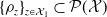 $\{ \rho _{z}\}_{z \in \mathcal{X}_1} \subset \mathcal{P}(\mathcal{X})$
and
$\{ \rho _{z}\}_{z \in \mathcal{X}_1} \subset \mathcal{P}(\mathcal{X})$
and
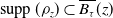 $\operatorname{supp}(\rho _{z}) \subset \overline {B_\tau } (z)$
. We further estimate,
$\operatorname{supp}(\rho _{z}) \subset \overline {B_\tau } (z)$
. We further estimate,
 \begin{align*} \int \int {E} ({x}) \text{d} \rho _{z} ({x}) \text{d} \mu (z) \geq \int {E}({r}_\tau (z)) \text{d} \mu (z)= \int {E}(z)\, \text{d} ({r}_\tau )_\# \mu (z), \end{align*}
and since
 $\tilde {\mu }$
was arbitrary, this concludes the proof.
$\tilde {\mu }$
was arbitrary, this concludes the proof.
In order to proceed with the following lemma, we also need the assumption that the potential is a
 $C^1$
-perturbation of a convex function and is Lipschitz continuous.
$C^1$
-perturbation of a convex function and is Lipschitz continuous.
Assumption 4.b.
Let
 ${E}\;:\;\mathcal{X} \rightarrow ({-}\infty ,+\infty ]$
be a
${E}\;:\;\mathcal{X} \rightarrow ({-}\infty ,+\infty ]$
be a
 $C^1$
-perturbation of a proper, convex lower semicontinuous function. Further, let the differentiable part
$C^1$
-perturbation of a proper, convex lower semicontinuous function. Further, let the differentiable part
 ${E}^{\text{d}}$
be globally Lipschitz.
${E}^{\text{d}}$
be globally Lipschitz.
Then the relation between the slope of
 $\mathcal{E}$
and the slope of the potential
$\mathcal{E}$
and the slope of the potential
 $E$
is stated in the following theorem.
$E$
is stated in the following theorem.
Lemma 4.17.
Let
 ${E}\;:\;\mathcal{X} \rightarrow ({-}\infty ,+\infty ]$
fulfil Assumptions 4.a and 4.b. Then
${E}\;:\;\mathcal{X} \rightarrow ({-}\infty ,+\infty ]$
fulfil Assumptions 4.a and 4.b. Then
 \begin{align} |\partial \mathcal{E}|(\mu )=\int _{\mathcal{X}} |\partial {E}|(x) \,\text{d}\mu (x) \end{align}
and
 $|\partial \mathcal{E}|(\mu )$
is a strong upper gradient of
$|\partial \mathcal{E}|(\mu )$
is a strong upper gradient of
 $\mathcal{E}$
.
$\mathcal{E}$
.
Proof. Since
 $\frac {{E}(x)-{E}_\tau (x)}{\tau }\geq 0$
we can use Fatou’s lemma to show
$\frac {{E}(x)-{E}_\tau (x)}{\tau }\geq 0$
we can use Fatou’s lemma to show
 \begin{align*} \int _{\mathcal{X}} |\partial {E}|(x) \,\text{d}\mu (x)&=\int _{\mathcal{X}} \lim _{\tau \rightarrow 0} \frac {{E}(x)-{E}_\tau (x)}{\tau } \,\text{d}\mu (x)\\&\leq \liminf _{\tau \rightarrow 0} \int _{\mathcal{X}} \frac {{E}(x)- {E}_\tau (x)}{\tau } \,\text{d}\mu (x)\\& \leq \limsup _{\tau \rightarrow 0} \int _{\mathcal{X}} \frac {{E}(x)-{E}({r}_\tau (x))}{\tau } \,\text{d}\mu (x)\\& = \limsup _{\tau \rightarrow 0} \frac {\mathcal{E}(\mu ) - \mathcal{E}(\mu _\tau )}{\tau } = |\partial \mathcal{E}|(\mu ), \end{align*}
where in the last step, we employ Lemma 2.8 . This implies that when
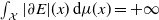 $\int _{\mathcal{X}} |\partial {E}|(x) \,\text{d}\mu (x)=+\infty$
then
$\int _{\mathcal{X}} |\partial {E}|(x) \,\text{d}\mu (x)=+\infty$
then
 $|\partial \mathcal{E}|(\mu )=+\infty$
. In the case
$|\partial \mathcal{E}|(\mu )=+\infty$
. In the case
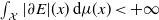 $\int _{\mathcal{X}} |\partial {E}|(x) \,\text{d}\mu (x)\lt +\infty$
, we use Lemma 2.8 (for
$\int _{\mathcal{X}} |\partial {E}|(x) \,\text{d}\mu (x)\lt +\infty$
, we use Lemma 2.8 (for
 $\mathcal{E}$
) and Lemma 3.5 (for
$\mathcal{E}$
) and Lemma 3.5 (for
 $E$
) to calculate
$E$
) to calculate
 \begin{align*} \int _{\mathcal{X}} |\partial {E}|(x) \,\text{d}\mu (x)&=\int _{\mathcal{X}} \lim _{\tau \rightarrow 0} \frac {{E}(x)- {E}_\tau (x)}{\tau }\,\text{d}\mu (x) \\ &=\lim _{\tau \rightarrow 0} \frac {\int _{\mathcal{X}} {E}(x)-{E}({r}_\tau (x)) \,\text{d}\mu (x)}{\tau }\\ &=\lim _{\tau \rightarrow 0} \frac {\mathcal{E}(\mu )-\mathcal{E}(\mu _\tau )}{\tau }=|\partial \mathcal{E}|(\mu ), \end{align*}
where the dominated convergence theorem was used to draw the limit into the integral. For the upper bound, we observe
 \begin{align*} |\partial {E}|(x)=&\limsup _{z\rightarrow x}\frac {({E}^{\text{c}}(x)-{E}^{\text{c}}(z)+{E}^{\text{d}}(x)-{E}^{\text{d}}(z))^+}{\|x-z\|}\\ \geq &\limsup _{z\rightarrow x} \frac {({E}^{\text{c}}(x)-{E}^{\text{c}}(z))^+}{\|x-z\|} -\frac {|{E}^{\text{d}}(x)-{E}^{\text{d}}(z)|}{\|x-z\|}\\ \geq &\limsup _{z\rightarrow x} \frac {({E}^{\text{c}}(x)-{E}^{\text{c}}(z))^+}{\|x-z\|}-\mathrm {Lip}({E}^{\text{d}})=|\partial {E}^{\text{c}}|(x)-\mathrm {Lip}({E}^{\text{d}}) \end{align*}
and by [Reference Ambrosio, Gigli and Savaré2, Theorem 2.4.9]
 \begin{equation*} \sup _{z\neq {x}}\frac {({E}^{\text{c}}({x})-{E}^{\text{c}}(z))^+}{\|{x}-z\|} =| \partial {E}^{\text{c}}|({x}).\end{equation*}
Then we can give an upper bound by
 \begin{align*} \frac {{E}(x)-{E}(r_\tau (x))}{\tau }&\leq \frac {{E}^{\text{c}}(x)-{E}^{\text{c}}(r_\tau (x))}{\|x-r_\tau (x)\|}+\frac {{E}^{\text{d}}(x)-{E}^{\text{d}}(r_\tau (x))}{\|x-r_\tau (x)\|} \\ &\leq \sup _{z\neq {x}}\frac {({E}^{\text{c}}(x)-{E}^{\text{c}}(z))^+}{\|x-z\|} +\mathrm {Lip}({E}^{\text{d}})=|\partial {E}^{\text{c}}|(x)+\mathrm {Lip}({E}^{\text{d}}) \\&\leq |\partial {E}|(x)+2\mathrm {Lip}({E}^{\text{d}}). \end{align*}
To prove that
 $|\partial \mathcal{E}|$
is a strong upper gradient, let
$|\partial \mathcal{E}|$
is a strong upper gradient, let
 $\mu _t$
be an absolutely continuous curve in
$\mu _t$
be an absolutely continuous curve in
 $\mathcal{W}_\infty (\mathcal{X})$
. Since
$\mathcal{W}_\infty (\mathcal{X})$
. Since
 $\left |\partial \mathcal{E}\right |(\mu )= \int _{\mathcal{X}} |\partial {E}|(x) \,\text{d}\mu ({x})$
and by Item 4 the slope
$\left |\partial \mathcal{E}\right |(\mu )= \int _{\mathcal{X}} |\partial {E}|(x) \,\text{d}\mu ({x})$
and by Item 4 the slope
 $|\partial {E}|(x)$
is lower semicontinuous, it follows from [Reference Ambrosio, Gigli and Savaré2, Lemma 5.1.7] that
$|\partial {E}|(x)$
is lower semicontinuous, it follows from [Reference Ambrosio, Gigli and Savaré2, Lemma 5.1.7] that
 $\left |\partial \mathcal{E}\right |(\mu )$
is lower semicontinuous w.r.t. narrow convergence and in particular
$\left |\partial \mathcal{E}\right |(\mu )$
is lower semicontinuous w.r.t. narrow convergence and in particular
 $t\mapsto |\partial \mathcal{E}|(\mu _t)$
is lower semicontinuous and thus Borel. Assume that
$t\mapsto |\partial \mathcal{E}|(\mu _t)$
is lower semicontinuous and thus Borel. Assume that
 $\int _s^t \int _{\mathcal{X}} |\partial {E}|(x) \,\text{d}\mu _r({x}) |\mu '|(r) \text{d}r = \int _s^t \left |\partial \mathcal{E}\right |(\mu _r) |\mu '|(r)\,\text{d}r\lt +\infty$
, otherwise (1.4) holds trivially. We can estimate
$\int _s^t \int _{\mathcal{X}} |\partial {E}|(x) \,\text{d}\mu _r({x}) |\mu '|(r) \text{d}r = \int _s^t \left |\partial \mathcal{E}\right |(\mu _r) |\mu '|(r)\,\text{d}r\lt +\infty$
, otherwise (1.4) holds trivially. We can estimate
 \begin{align} \begin{split} |\mathcal{E}(\mu _t)-\mathcal{E}(\mu _s)|&=\left |\int _{\mathcal{X}} {E}(x)\,\text{d}\mu _t(x)-\int _{\mathcal{X}} {E}(x)\,\text{d}\mu _s(x)\right |\\ &=\left |\int _{\mathcal{X}} {E}({x})\text{d}{e_t}_\# \eta ({x})-\int _{\mathcal{X}} {E}({x})\text{d}{e_s}_\# \eta ({x})\right |\\ &=\left |\int _{C(0,T;\;\mathcal{X})} {E}(u(t))\,\text{d}\eta (u)-\int _{C(0,T;\;\mathcal{X})} {E}(u(s))\text{d} \eta (u)\right | \\&\leq \int _{C(0,T;\;\mathcal{X})} |{E}(u(t))-{E}(u(s))| \,\text{d}\eta (u)\\ &\overset {(i)}{\leq }\int _{C(0,T;\;\mathcal{X})} \int _s^t | \partial {E}|(u(r))\, |u'|(r)\,\text{d}r \,\text{d}\eta (u)\\ &\overset {(ii)}{=}\int _s^t\int _{C(0,T;\;\mathcal{X})} | \partial {E}|(u(r))\, |u'|(r) \,\text{d}\eta (u)\,\text{d}r\\ &\overset {(iii)}{\leq } \int _s^t\int _{C(0,T;\;\mathcal{X})} | \partial {E}|(u(r)) \,\text{d}\eta (u) |\mu '|(r)\,\text{d}r\\ &= \int _s^t\int _{\mathcal{X}} | \partial {E}|(x) \,\text{d}\mu _r |\mu '|(r)\,\text{d}r\lt +\infty , \end{split} \end{align}
where
 $(t,u)\mapsto | \partial {E}|(u(t))$
is
$(t,u)\mapsto | \partial {E}|(u(t))$
is
 $\bar {\eta }$
-measurable since it is lower semicontinuous on
$\bar {\eta }$
-measurable since it is lower semicontinuous on
 $[0,T]\times C(0,T,\mathcal{X})$
and measurability of
$[0,T]\times C(0,T,\mathcal{X})$
and measurability of
 $\left |u'\right |$
follows as in the proof of [Reference Lisini62, Theorem 7] and Theorem 4.9. For
$\left |u'\right |$
follows as in the proof of [Reference Lisini62, Theorem 7] and Theorem 4.9. For
 $(ii)$
, we use the theorem of Fubini–Tonelli, while for
$(ii)$
, we use the theorem of Fubini–Tonelli, while for
 $(i)$
, we observe that
$(i)$
, we observe that
 $\eta$
from Theorem 4.7 is concentrated on
$\eta$
from Theorem 4.7 is concentrated on
 ${\mathrm{AC}}^\infty (0,T;\;\mathcal{X})$
and
${\mathrm{AC}}^\infty (0,T;\;\mathcal{X})$
and
 $|\partial {E}|$
is a strong upper gradient (c.f. Definition 1.4) and for (iii) we use
$|\partial {E}|$
is a strong upper gradient (c.f. Definition 1.4) and for (iii) we use
 $|\mu '|(t)=\| |u'|(t)\|_{L_p(\eta )}$
.
$|\mu '|(t)=\| |u'|(t)\|_{L_p(\eta )}$
.
The main result of this section now states that
 $\infty$
-curves of maximal slope on
$\infty$
-curves of maximal slope on
 $W_\infty (\mathcal{X})$
can be equivalently characterized, by the property that
$W_\infty (\mathcal{X})$
can be equivalently characterized, by the property that
 $\eta$
-a.e. curve fulfils the differential inclusion w.r.t. the potential
$\eta$
-a.e. curve fulfils the differential inclusion w.r.t. the potential
 $E$
on the Banach space
$E$
on the Banach space
 $\mathcal{X}$
.
$\mathcal{X}$
.
Theorem 4.18.
Let
 $\mathcal{E}\;:\; W_\infty (\mathcal{X})\rightarrow ({-}\infty ,+\infty ]$
be a potential energy with the potential
$\mathcal{E}\;:\; W_\infty (\mathcal{X})\rightarrow ({-}\infty ,+\infty ]$
be a potential energy with the potential
 $E$
satisfying Assumptions 4.a and 4.b,
$E$
satisfying Assumptions 4.a and 4.b,
 $\mu _t \in \operatorname {dom}(\mathcal{E})$
for all
$\mu _t \in \operatorname {dom}(\mathcal{E})$
for all
 $t\in [0,T]$
and
$t\in [0,T]$
and
 $\mu \in {\mathrm{AC}}^\infty (0,T; \mathcal{W}_\infty )$
with
$\mu \in {\mathrm{AC}}^\infty (0,T; \mathcal{W}_\infty )$
with
 $\eta$
from Theorem 4.7
. Let further
$\eta$
from Theorem 4.7
. Let further
 $\mathcal{E}\circ \mu$
be for a.e.
$\mathcal{E}\circ \mu$
be for a.e.
 $t\in [0,T]$
equal to a non-increasing map
$t\in [0,T]$
equal to a non-increasing map
 $\psi \;:\;[0,T] \rightarrow {\mathbb{R}}$
. Then the following statements are equivalent:
$\psi \;:\;[0,T] \rightarrow {\mathbb{R}}$
. Then the following statements are equivalent:
-
(i)
$|\mu '|(t)\leq 1 \text{ and } \psi '(t)\leq -|\partial \mathcal{E}|(\mu (t)) \text{ for a.e. } t\in (0,T).$
-
(i) For
$\eta$
-a.e. curve
$u\in C(0,T;\;\mathcal{X})$
it holds, that
$E\circ u$
is for a.e.
$t\in (0,T)$
equal to a non-increasing map
$\psi _u: [0,T]\rightarrow {\mathbb{R}}$
and
\begin{equation*} u'(t)\ \in \ \partial \|\cdot \|_*({-}\xi ) \quad \forall \xi \in \partial ^\circ {E}(u(t)) \not = \emptyset , \quad \text{for a.e. } t\in (0,T).\end{equation*}


Proof. Step 1:
 $(\text{i})\Longrightarrow (\text{ii})$
.
$(\text{i})\Longrightarrow (\text{ii})$
.
Because of Remark 2.3 we know that
 $\mu _t$
satisfies the energy dissipation equality (2.10). Making a similar estimate as in (4.13), we obtain
$\mu _t$
satisfies the energy dissipation equality (2.10). Making a similar estimate as in (4.13), we obtain
 \begin{align} \begin{split} \mathcal{E}(\mu _0)-\mathcal{E}(\mu _T)&= \int _{C(0,T;\;\mathcal{X})} E(u(0))-E(u(T)) \,\text{d}\eta (u)\\ &\leq \int _{C(0,T;\;\mathcal{X})} \int _0^T |\partial E|(u(r)) |u'|(t) \,\text{d}r \,\text{d}\eta (u)\\ &\leq \int _{C(0,T;\;\mathcal{X})} \int _0^T |\partial E|(u(r)) \,\text{d}r \,\text{d}\eta (u)\\ &=\int _0^T |\partial \mathcal{E}|(\mu (r))\,\text{d}r=\mathcal{E}(\mu _0)-\mathcal{E}(\mu _T). \end{split} \end{align}
This implies that
 $|\partial E|(u(r))|u'|(t) \in L^1(0,T)$
for
$|\partial E|(u(r))|u'|(t) \in L^1(0,T)$
for
 $\eta$
-a.e.
$\eta$
-a.e.
 $u$
. Since
$u$
. Since
 $|\partial E|$
is a strong upper gradient
$|\partial E|$
is a strong upper gradient
 $\psi _u:t\mapsto E(u(t))$
has to be absolutely continuous for
$\psi _u:t\mapsto E(u(t))$
has to be absolutely continuous for
 $\eta$
-a.e.
$\eta$
-a.e.
 $u$
and
$u$
and
 \begin{align*} E(u(s))-E(u(t))\leq \int _s^t |\partial E|(u(r)) |u'|(r) \,\text{d}r \leq \int _s^t |\partial E|(u(r)) \,\text{d}r \quad \text{for }\eta \text{-a.e. }u \text{ for all } 0 \leq s \lt t \leq T. \end{align*}
Equality in (4.14) can then only hold if for all
 $0\leq s \lt t \leq T$
we have
$0\leq s \lt t \leq T$
we have
 \begin{align*} E(u(s))-E(u(t))= \int _s^t |\partial E|(u(r)) |u'|(t) \,\text{d}r = \int _s^t |\partial E|(u(r)) \,\text{d}r \quad \text{for }\eta \text{-a.e. }u \end{align*}
and thus
 $\psi _u \;:\!=\; E\circ u$
is a non-increasing map for
$\psi _u \;:\!=\; E\circ u$
is a non-increasing map for
 $\eta$
-a.e.
$\eta$
-a.e.
 $u$
. Lemma 3.7 and Item 3 imply that for every
$u$
. Lemma 3.7 and Item 3 imply that for every
 $\xi \in \partial ^\circ {E}(u(t))$
we obtain
$\xi \in \partial ^\circ {E}(u(t))$
we obtain
 \begin{align*} \langle \xi , u'(t)\rangle = ({E}\circ u)'(t) = -|\partial {E}|(u(t)) =-\left \|\xi \right \|_*-\chi _{\overline {B_1}}(u'(t)), \end{align*}
where we use Lemma E.4 and
 $ \||u'|(t)\|_{L^\infty (\eta )}=|\mu '|(t)\leq 1$
for a.e.
$ \||u'|(t)\|_{L^\infty (\eta )}=|\mu '|(t)\leq 1$
for a.e.
 $t\in (0,T)$
to infer that
$t\in (0,T)$
to infer that
 $\left |u'\right |(t)\leq 1$
for a.e.
$\left |u'\right |(t)\leq 1$
for a.e.
 $t\in (0,T)$
. Using the equivalence of Item 3 and Item 1 yields
$t\in (0,T)$
. Using the equivalence of Item 3 and Item 1 yields
 \begin{align*} u'(t) \in \partial \left \|\cdot \right \|_*({-}\xi ) \end{align*}
for a.e.
 $t\in (0,T)$
and
$t\in (0,T)$
and
 $\eta$
-a.e. curve
$\eta$
-a.e. curve
 $u$
.
$u$
.
Step 2:
 $(\text{ii})\Longrightarrow (\text{i})$
.
$(\text{ii})\Longrightarrow (\text{i})$
.
Due to Remark 2.3,
 $E\circ u$
is for
$E\circ u$
is for
 $\eta$
-a.e. curve
$\eta$
-a.e. curve
 $u\in C(0,T;\;\mathcal{X})$
an absolutely continuous curve, and it satisfies the energy dissipation equality
$u\in C(0,T;\;\mathcal{X})$
an absolutely continuous curve, and it satisfies the energy dissipation equality
 \begin{align*} E(u(t))-E(u(s))=\int _s^t -|\partial E|(u(r)) \,\text{d}r \quad \text{for }0\leq s\leq t\leq T. \end{align*}
Therefore, we obtain
 \begin{align*} \mathcal{E}(\mu _t) - \mathcal{E}(\mu _s) &= \int _{C(0,T;\;\mathcal{X})} E(u(t))-E(u(s)) \,\text{d}\eta (u) = \int _{C(0,T;\;\mathcal{X})} \int _s^t -|\partial E|(u(r)) \,\text{d}r \,\text{d}\eta (u)\\ &= \int _s^t \int _{C(0,T;\;\mathcal{X})} -|\partial E|(u(r)) \,\text{d}\eta (u)\,\text{d}r = \int _s^t -\left |\partial \mathcal{E}\right |(\mu _r) \,\text{d}r\leq 0, \end{align*}
where the application of Fubini–Tonelli is justified due to the assumption
 $\mu _t\in \operatorname {dom}(\mathcal{E})$
for all
$\mu _t\in \operatorname {dom}(\mathcal{E})$
for all
 $t\in [0,T]$
, which yields that
$t\in [0,T]$
, which yields that
 $\left |\mathcal{E}(\mu _t) - \mathcal{E}(\mu _s)\right | \lt \infty$
for all
$\left |\mathcal{E}(\mu _t) - \mathcal{E}(\mu _s)\right | \lt \infty$
for all
 $s,t\in [0,T]$
. By the Lebesgue differentiation theorem, we obtain
$s,t\in [0,T]$
. By the Lebesgue differentiation theorem, we obtain
 \begin{align*} (\mathcal{E}\circ \mu )'(t) = -\left |\partial \mathcal{E}\right |(\mu _t) \end{align*}
for almost every
 $t\in (0,T)$
. Furthermore,
$t\in (0,T)$
. Furthermore,
 $\mathcal{E} \circ \mu$
is a non-increasing map and Theorem 4.7 yields that
$\mathcal{E} \circ \mu$
is a non-increasing map and Theorem 4.7 yields that
 \begin{align*} \left |\mu '\right |(t) = \eta (u) -\operatorname{ess\,sup} \left |u'\right |(t) \leq 1 \end{align*}
for a.e.
 $t\in (0,T)$
and since
$t\in (0,T)$
and since
 $\mu \in {\mathrm{AC}}^\infty$
this yields that
$\mu \in {\mathrm{AC}}^\infty$
this yields that
 $\left |\mu '\right |(t)\leq 1$
for a.e.
$\left |\mu '\right |(t)\leq 1$
for a.e.
 $t\in (0,T)$
.
$t\in (0,T)$
.
Remark 4.19. In particular, those curves of maximal slope satisfy the continuity equation for the velocity field
 \begin{equation*} \boldsymbol{v} _t(x)\;:\!=\; \int _{C(0,T;\;\mathcal{X})} u'(t) \text{d} \bar {\eta }_{x,t} \quad \text{for } \bar {\mu } \text{-a.e. } (t,x) \in (0,T)\times \mathcal{X}.\end{equation*}
If
 $\partial ^\circ {E}(x)$
is unique, i.e., if
$\partial ^\circ {E}(x)$
is unique, i.e., if
 $\|\cdot \|$
is strictly convex or
$\|\cdot \|$
is strictly convex or
 $E(x)\in C^1(\mathcal{X})$
, then for
$E(x)\in C^1(\mathcal{X})$
, then for
 $\bar {\eta }_{x,t}$
-a.e.
$\bar {\eta }_{x,t}$
-a.e.
 $u\in C(0,T;\;\mathcal{X})$
the derivatives
$u\in C(0,T;\;\mathcal{X})$
the derivatives
 $u'(t)$
lie in the closed and convex set
$u'(t)$
lie in the closed and convex set
 $\partial \|\cdot \|_*({-}\partial ^\circ E(x))$
. Thus
$\partial \|\cdot \|_*({-}\partial ^\circ E(x))$
. Thus
 \begin{equation*} \boldsymbol{v} _t(x)\in \partial \|\cdot \|_*({-}\partial ^\circ E(x))\quad \text{for } \bar {\mu } \text{-a.e. } (t,x) \in (0,T)\times \mathcal{X}.\end{equation*}
As the last result in this section, we give an explicit setting where the existence of curves of maximum slope is ensured. Here, we restrict ourselves to finite dimensions, mimicking Corollary 3.2.
Corollary 4.20 (Existence in finite dimensions). Let
 $\mathcal{X}=(\mathbb{R}^d, \|\cdot \|)$
and
$\mathcal{X}=(\mathbb{R}^d, \|\cdot \|)$
and
 ${E}\;:\;{\mathbb{R}}^d \to ({-}\infty ,\infty ]$
be a
${E}\;:\;{\mathbb{R}}^d \to ({-}\infty ,\infty ]$
be a
 $C^1$
-perturbation of a proper, lower semicontinuous, convex function. For every
$C^1$
-perturbation of a proper, lower semicontinuous, convex function. For every
 $\mu ^0\in \operatorname {dom}(\mathcal{E})$
, there exists at least one curve of maximal slope in the sense of Definition 2.1
with
$\mu ^0\in \operatorname {dom}(\mathcal{E})$
, there exists at least one curve of maximal slope in the sense of Definition 2.1
with
 $\mu _0=\mu ^0$
. Further, this curve satisfies the energy dissipation equality (2.10).
$\mu _0=\mu ^0$
. Further, this curve satisfies the energy dissipation equality (2.10).
Proof. We simply check the conditions of Theorem 2.11. Choosing
 $\sigma$
to be the narrow topology, Lemma 4.5 guarantees Assumption 1.a. To check Assumption 1.b, we know that for any sequence
$\sigma$
to be the narrow topology, Lemma 4.5 guarantees Assumption 1.a. To check Assumption 1.b, we know that for any sequence
 $\left (\mu ^{n}\right )_{n\in \mathbb{N}}$
,
$\left (\mu ^{n}\right )_{n\in \mathbb{N}}$
,
 $W_\infty (\mu ^k,\mu ^m)\lt \infty \quad \forall k,m\in \mathbb{N}$
implies that
$W_\infty (\mu ^k,\mu ^m)\lt \infty \quad \forall k,m\in \mathbb{N}$
implies that
 $\cup _{n} supp(\mu ^n)$
is bounded. Since we are in the finite dimensional case, we can now apply Prokhorov’s Theorem to obtain relative compactness of the sequence.
$\cup _{n} supp(\mu ^n)$
is bounded. Since we are in the finite dimensional case, we can now apply Prokhorov’s Theorem to obtain relative compactness of the sequence.
We are left to check Assumptions 2.a and 2.b for
 $\mathcal{E}$
:
$\mathcal{E}$
:
Assumption 2.a
Let
 $\mu ^n\in \operatorname {dom}(\mathcal{E})$
be a sequence converging in
$\mu ^n\in \operatorname {dom}(\mathcal{E})$
be a sequence converging in
 $W_\infty$
to
$W_\infty$
to
 $\mu$
. This sequence has to be bounded in
$\mu$
. This sequence has to be bounded in
 $W_\infty$
such that
$W_\infty$
such that
 $\overline {\cup _n \operatorname{supp}(\mu ^n)}$
is bounded. Since
$\overline {\cup _n \operatorname{supp}(\mu ^n)}$
is bounded. Since
 $E$
is lower-semicontinuous
$E$
is lower-semicontinuous
 $\operatorname {dom}(E)$
is closed and thus
$\operatorname {dom}(E)$
is closed and thus
 $\overline {\cup _n \operatorname{supp}(\mu ^n)}\cap \operatorname {dom}({E})$
is compact and we obtain due to lower-semicontinuity
$\overline {\cup _n \operatorname{supp}(\mu ^n)}\cap \operatorname {dom}({E})$
is compact and we obtain due to lower-semicontinuity
 \begin{align*} \min _{x\in \overline {\cup _n \operatorname*{supp}(\mu ^n)}\cap \operatorname {dom}({E})}{E}(x)\gt -\infty \end{align*}
Thus the negative part of
 ${E}(x)$
denoted by
${E}(x)$
denoted by
 ${E}^-(x)$
is uniformly integrable with respect to
${E}^-(x)$
is uniformly integrable with respect to
 $\{\mu ^n\}_{n\in \mathbb{N}}$
and we can apply [Reference Ambrosio, Gigli and Savaré2, Lemma 5.1.7] to obtain
$\{\mu ^n\}_{n\in \mathbb{N}}$
and we can apply [Reference Ambrosio, Gigli and Savaré2, Lemma 5.1.7] to obtain
 \begin{equation*}\liminf _{n\rightarrow \infty } \int {E}(x)\,\text{d}\mu ^n(x)\geq \int {E}(x) \,\text{d}\mu . \end{equation*}
Assumption 2.b:
Since
 $\mu$
has bounded domain the differentiable part
$\mu$
has bounded domain the differentiable part
 $E^d$
satisfies a Lischitz condition and thus by Lemma 4.17
$E^d$
satisfies a Lischitz condition and thus by Lemma 4.17
 \begin{equation*}|\partial \mathcal{E}|(\mu )=\int |\partial {E}|(x) \,\text{d}\mu \end{equation*}
and by Proposition 3.1
 $|\partial {E}|(x)$
is lower semicontinuous and non-negative. Thus
$|\partial {E}|(x)$
is lower semicontinuous and non-negative. Thus
 $|\partial {E}|(x)$
is uniformly integral, and we can apply [Reference Ambrosio, Gigli and Savaré2, Lemma 5.1.7] to obtain
$|\partial {E}|(x)$
is uniformly integral, and we can apply [Reference Ambrosio, Gigli and Savaré2, Lemma 5.1.7] to obtain
 \begin{equation*}\liminf _{n\rightarrow \infty } \int |\partial {E}|(x)\,\text{d}\mu ^n \geq \int |\partial {E}|(x)\,\text{d}\mu \end{equation*}
for all
 $\mu ^n$
converging narrowly to
$\mu ^n$
converging narrowly to
 $\mu$
.
$\mu$
.
5. Relation to adversarial attacks
This section explores the connection of the previous results to our initial motivation, adversarial attacks. As mentioned before, we now consider an energy defined as
 \begin{align*} E({x}) \;:\!=\; -\ell (h({x}), y) \end{align*}
for a classifier
 $h$
and
$h$
and
 ${x}\in \mathcal{X}, y\in \mathcal{Y}$
. The goal in (AdvAtt) is to maximize this function on the set
${x}\in \mathcal{X}, y\in \mathcal{Y}$
. The goal in (AdvAtt) is to maximize this function on the set
 $\overline {B_\varepsilon }({x}^0)$
, where
$\overline {B_\varepsilon }({x}^0)$
, where
 ${x}^0\in \mathcal{X}$
is the initial input. Roughly following the idea in the original paper proposing (FGSM), we derive the scheme, via linearizing
${x}^0\in \mathcal{X}$
is the initial input. Roughly following the idea in the original paper proposing (FGSM), we derive the scheme, via linearizing
 $E$
around
$E$
around
 ${x}^0$
and consider the linearized minimizing movement scheme in Definition 3.10. Assuming that
${x}^0$
and consider the linearized minimizing movement scheme in Definition 3.10. Assuming that
 $\ell (h(\cdot ), y)$
is
$\ell (h(\cdot ), y)$
is
 $C^1$
, we consider
$C^1$
, we consider
 \begin{align*} E^{\mathrm{sl}}({x}; z)= -\ell (h(z),y)- \langle \nabla _{x} \ell (h(z),y),{x}-z\rangle , \end{align*}
where
 $z$
denotes the point of linearization. Lemma 3.12 yields that the semi-implicit minimizing movement scheme in Definition 3.10 can be expressed as
$z$
denotes the point of linearization. Lemma 3.12 yields that the semi-implicit minimizing movement scheme in Definition 3.10 can be expressed as
 \begin{align*} x_{\mathrm {si},\tau }^{k+1} \in x_{\mathrm {si},\tau }^{k}-\tau \partial \left \|\cdot \right \|_*(D E(x_{\mathrm {si},\tau }^{k})). \end{align*}
We note that this scheme can be understood as an explicit Euler discretization [Reference Euler38] of the differential inclusion in Theorem 3.8,
 \begin{align} u'(t)\in \operatorname*{arg\,max}_{{x}\in \overline {B_1}} \langle {x}, -D E(u(t))\rangle = \partial \left \|\cdot \right \|_*(D E(u(t))), \end{align}
which in turn is an equivalent characterization of
 $\infty$
-curves of maximal slope. In this section, we consider the finite dimensional adversarial setting, i.e., the Banach space
$\infty$
-curves of maximal slope. In this section, we consider the finite dimensional adversarial setting, i.e., the Banach space
 $(\mathcal{X}, \left \|\cdot \right \|) = ({\mathbb{R}}^d, \left \|\cdot \right \|_p)$
.
$(\mathcal{X}, \left \|\cdot \right \|) = ({\mathbb{R}}^d, \left \|\cdot \right \|_p)$
.
Corollary 5.1.
Given
 ${x}^0\in {\mathbb{R}}^d$
, the iteration
${x}^0\in {\mathbb{R}}^d$
, the iteration
 \begin{align*} x_{\mathrm {si},\tau }^{k+1} = x_{\mathrm {si},\tau }^k + \tau \ \operatorname {sign}(\nabla _x E(x_{\mathrm {si},\tau }^k))\cdot \left (\frac {\left |\nabla _x E(x_{\mathrm {si},\tau }^k)\right |}{\left \|\nabla _x E(x_{\mathrm {si},\tau }^k)\right \|_q}\right )^{q-1}, \qquad x_{\mathrm {si},\tau }^0 = {x}^0 \end{align*}
fulfils the semi-implicit minimizing movement scheme in Definition 3.10
in the space
 $({\mathbb{R}}^d, \left \|\cdot \right \|_p)$
with
$({\mathbb{R}}^d, \left \|\cdot \right \|_p)$
with
 $1/p + 1/q=1$
. In this sense, (FGSM) is a one-step explicit Euler discretization of the differential inclusion (5.1) with step size
$1/p + 1/q=1$
. In this sense, (FGSM) is a one-step explicit Euler discretization of the differential inclusion (5.1) with step size
 $\varepsilon$
.
$\varepsilon$
.
Remark 5.2. We note that for
 $p\in \{1,\infty \}$
, the expression in Corollary 5.1 is to be understood in the sense of subdifferentials, as the following proof shows. However, the elements of the subdifferential we choose can be understood as the limit cases of
$p\in \{1,\infty \}$
, the expression in Corollary 5.1 is to be understood in the sense of subdifferentials, as the following proof shows. However, the elements of the subdifferential we choose can be understood as the limit cases of
 $p\to 1$
and
$p\to 1$
and
 $p\to \infty$
, respectively.
$p\to \infty$
, respectively.
Proof. We choose
 $\mathcal{X}={\mathbb{R}}^d$
with
$\mathcal{X}={\mathbb{R}}^d$
with
 $\left \|\cdot \right \| = \left \|\cdot \right \|_{p}$
. For
$\left \|\cdot \right \| = \left \|\cdot \right \|_{p}$
. For
 $p=\infty$
, we have that
$p=\infty$
, we have that
 \begin{align*} \operatorname {sign}(\xi ) \in \partial \left \|\cdot \right \|_{1}(\xi ) = \partial (\left \|\cdot \right \|_{\infty })_*(\xi ), \end{align*}
for all
 $\xi \in {\mathbb{R}}^d$
and therefore, the following iteration fulfils the semi-implicit minimizing movement scheme,
$\xi \in {\mathbb{R}}^d$
and therefore, the following iteration fulfils the semi-implicit minimizing movement scheme,
 \begin{align*} x_{\mathrm {si},\tau }^{k+1} = x_{\mathrm {si},\tau }^{k} - \tau \operatorname {sign}(\nabla _{x} E (x_{\mathrm {si},\tau }^{k})) = x_{\mathrm {si},\tau }^{k} + \varepsilon \operatorname {sign}(\nabla _{x} \ell (h(x_{\mathrm {si},\tau }^{k}), y)) , \end{align*}
and for
 $\varepsilon =\tau$
the statement follows. For
$\varepsilon =\tau$
the statement follows. For
 $p=1$
, we choose the following element of the subdifferential
$p=1$
, we choose the following element of the subdifferential
 $g(\xi )$
, with
$g(\xi )$
, with
 \begin{align*} g(\xi )_i \;:\!=\; \#\{j\;:\;\left |\xi _j\right | = \left \|\xi \right \|_\infty \}^{-1} \cdot \begin{cases} \operatorname {sign}(\xi _i) &\text{if} \left |\xi _i\right |= \left \|\xi \right \|_\infty ,\\ 0&\text{else}, \end{cases} \end{align*}
and proceed as before. If we instead choose a finite
 $p\in (1,\infty )$
, we obtain for
$p\in (1,\infty )$
, we obtain for
 $1/p + 1/q=1$
,
$1/p + 1/q=1$
,
 \begin{align*} \partial (\left \|\cdot \right \|_p)_*(\xi ) = \partial \left \|\cdot \right \|_q(\xi ) = \left \|\xi \right \|_q^{1-q} (\xi _1 \left |\xi _1\right |^{q-2},\ldots , \xi _d\left |\xi _d\right |^{q-2}) = \operatorname {sign}(\xi )\cdot \left (\frac {\left |\xi \right |}{\left \|\xi \right \|_q}\right )^{q-1}, \end{align*}
where the absolute value and the multiplication is to be understood entrywise. As above, this yields the statement also for
 $p\in (1,\infty )$
.
$p\in (1,\infty )$
.
5.1. Convergence of IFGSM to curves of maximal slope
Our main goal is to derive a convergence result of (IFGSM) for
 $\tau \to 0$
. As mentioned before, Lemma 3.12 yields an iteration, which can be expressed as normalized gradient descent in the finite-dimensional case. The main obstacle that prohibits us from directly applying the convergence result for semi-implicit schemes (see Theorem 3.16) is the budget constraint,
$\tau \to 0$
. As mentioned before, Lemma 3.12 yields an iteration, which can be expressed as normalized gradient descent in the finite-dimensional case. The main obstacle that prohibits us from directly applying the convergence result for semi-implicit schemes (see Theorem 3.16) is the budget constraint,
 $u'(t)\in \overline {B_\varepsilon ^p}({x}^0)$
for all
$u'(t)\in \overline {B_\varepsilon ^p}({x}^0)$
for all
 $t$
. Here and in the following, we now assume that the norm exponent of the underlying space and of the budget constraint norm are the same. In (IFGSM), this is enforced via a projection onto this set in each iteration. An easy way to circumvent this issue is to only consider the iteration up to the step, where it would leave the constraint set. In this case, the projection never has any effect and we essentially consider signed gradient descent. Intuitively, the Lipschitz condition
$t$
. Here and in the following, we now assume that the norm exponent of the underlying space and of the budget constraint norm are the same. In (IFGSM), this is enforced via a projection onto this set in each iteration. An easy way to circumvent this issue is to only consider the iteration up to the step, where it would leave the constraint set. In this case, the projection never has any effect and we essentially consider signed gradient descent. Intuitively, the Lipschitz condition
 $\left \|u'(t)\right \|\leq 1$
allows us to control how far
$\left \|u'(t)\right \|\leq 1$
allows us to control how far
 $u(t)$
is away from
$u(t)$
is away from
 ${x}^0$
. This mimicked in the discrete scheme, where we know that
${x}^0$
. This mimicked in the discrete scheme, where we know that
 \begin{align*} \left \|x_{\mathrm {si},\tau }^{i} - {x}^0\right \|\leq \sum _{k=0}^{n-1} \left \|x_{\mathrm {si},\tau }^{k+1} - x_{\mathrm {si},\tau }^{k}\right \|\leq n\tau = T, \end{align*}
for every
 $i=0,\ldots , n$
. Therefore, we can choose
$i=0,\ldots , n$
. Therefore, we can choose
 $T=\varepsilon$
to ensure that
$T=\varepsilon$
to ensure that
 $x_{\mathrm {si},\tau }^{i}\in \overline {B_\varepsilon ^p}({x}^0)$
for every
$x_{\mathrm {si},\tau }^{i}\in \overline {B_\varepsilon ^p}({x}^0)$
for every
 $i=0,\ldots ,n$
. This yields the following result.
$i=0,\ldots ,n$
. This yields the following result.
Corollary 5.3.
We consider the space
 $(\mathcal{X}, \left \|\cdot \right \|) = ({\mathbb{R}}^d, \left \|\cdot \right \|_{p})$
for
$(\mathcal{X}, \left \|\cdot \right \|) = ({\mathbb{R}}^d, \left \|\cdot \right \|_{p})$
for
 $p\in [1,\infty ]$
and
$p\in [1,\infty ]$
and
 $E\;:\;{\mathbb{R}}^d\to {\mathbb{R}}$
, a continuously differentiable energy, with a Lipschitz continuous gradient. Then for
$E\;:\;{\mathbb{R}}^d\to {\mathbb{R}}$
, a continuously differentiable energy, with a Lipschitz continuous gradient. Then for
 $T=\varepsilon$
, there exists a
$T=\varepsilon$
, there exists a
 $\infty$
-curve of maximal slope
$\infty$
-curve of maximal slope
 $u\;:\;[0,T]\to {\mathbb{R}}^d$
, with respect to
$u\;:\;[0,T]\to {\mathbb{R}}^d$
, with respect to
 $E$
, and a subsequence of
$E$
, and a subsequence of
 $\tau _n\;:\!=\;T/n$
such that
$\tau _n\;:\!=\;T/n$
such that
 \begin{align*} \left \|u_{\mathrm{IFGS}, \tau _{n_i}}^{\lceil t/\tau _{n_i} \rceil } - u(t)\right \|\xrightarrow {i\to \infty } 0\qquad \text{ for all } t\in [0,T]. \end{align*}
Proof. From Lemma 3.12 and the calculation in the proof of Corollary 5.1, we know that the iterates of (IFGSM) fulfil the linearized minimizing movement scheme in Definition 3.10. Here, we used that for
 $T=\varepsilon$
, the iterates do not leave the set
$T=\varepsilon$
, the iterates do not leave the set
 $\overline {B_\varepsilon ^p}({x}^0)$
and therefore the projection has no effect. Assumption 3.a is stated as an assumption of this corollary and Remark 3.9 yields that Assumption 3.b holds true. Furthermore, using Proposition 3.1, we know that Assumptions 1.a to 2.b are fulfilled, and therefore, we can apply Theorem 3.16 to obtain the desired result.
$\overline {B_\varepsilon ^p}({x}^0)$
and therefore the projection has no effect. Assumption 3.a is stated as an assumption of this corollary and Remark 3.9 yields that Assumption 3.b holds true. Furthermore, using Proposition 3.1, we know that Assumptions 1.a to 2.b are fulfilled, and therefore, we can apply Theorem 3.16 to obtain the desired result.
Above, we only consider convergence up to a subsequence. While the convergence of the whole sequence for (IFGSM) is left unanswered in this work, we note that at least for
 $p\in \{1,\infty \}$
, this cannot be expected, since in this case
$p\in \{1,\infty \}$
, this cannot be expected, since in this case
 $\infty$
-curves of maximal slope lack uniqueness, even in the simple finite dimensional case, as the following example shows.
$\infty$
-curves of maximal slope lack uniqueness, even in the simple finite dimensional case, as the following example shows.
Example 4 (Non uniqueness for
 $p\in \{1,\infty \}$
). Let
$p\in \{1,\infty \}$
). Let
 $(\mathcal{X},\left \|\cdot \right \|)=({\mathbb{R}}^2,\left \|\cdot \right \|_\infty )$
and consider the energy be given by
$(\mathcal{X},\left \|\cdot \right \|)=({\mathbb{R}}^2,\left \|\cdot \right \|_\infty )$
and consider the energy be given by
 \begin{equation*} E\;:\;(x_1,x_2)\in {\mathbb{R}}^2\mapsto x_1\in {\mathbb{R}} \end{equation*}
then both
 $u_1(t)=({-}t,0)$
and
$u_1(t)=({-}t,0)$
and
 $u_2(t)=({-}t,-t)$
are
$u_2(t)=({-}t,-t)$
are
 $\infty$
-curves of maximal slope on
$\infty$
-curves of maximal slope on
 $[0,T],T\gt 0$
, with
$[0,T],T\gt 0$
, with
 $u_1(0)=u_2(0)$
since
$u_1(0)=u_2(0)$
since
 \begin{equation*}u_1'(t)=({-}1,0)\in -\partial \left \|\cdot \right \|_1(1,0)=-\partial \left \|\cdot \right \|_1(\nabla E(u_1(t)))\end{equation*}
and
 \begin{equation*}u_2'(t)=({-}1,-1)\in -\partial \left \|\cdot \right \|_1(1,0)= -\partial \left \|\cdot \right \|_1(\nabla E(u_2(t))).\end{equation*}
In two dimensions for
 $p=1$
, we can simply rotate the above setup to deduce the same non-uniqueness. Namely for
$p=1$
, we can simply rotate the above setup to deduce the same non-uniqueness. Namely for
 $ E({x}_1,{x}_2)={x}_1+{x}_2$
, we have that
$ E({x}_1,{x}_2)={x}_1+{x}_2$
, we have that
 $u_1(t) = ({-}t,0)$
fulfils
$u_1(t) = ({-}t,0)$
fulfils
 \begin{equation*}u_1'(t)=({-}1,0)\in -\partial \left \|\cdot \right \|_\infty (1,1)=-\partial \left \|\cdot \right \|_\infty (\nabla E(u_1(t))) \end{equation*}
and also
 $u_2(t) = \frac {1}{2}({-}t,-t)$
fulfils
$u_2(t) = \frac {1}{2}({-}t,-t)$
fulfils
 \begin{equation*}u_2'(t)=\frac {1}{2}({-}1,-1)\in -\partial \left \|\cdot \right \|_\infty (1,1)=-\partial \left \|\cdot \right \|_\infty (\nabla E(u_2(t))). \end{equation*}
In Corollary 5.3, we only allow the iteration to run until it hits the boundary. However, in practice, it is more common to also iterate beyond the time
 $\varepsilon$
. In order to incorporate the budget constraint in this case, we modify the energy to
$\varepsilon$
. In order to incorporate the budget constraint in this case, we modify the energy to
 \begin{align*} E ({x}) \;:\!=\; -\ell (h({x}), y) + \chi _{\overline {B_\varepsilon ^p}({x}^0)}({x}), \end{align*}
which yields the semi-implicit energy
 \begin{align*} E^{\mathrm{sl}}({x};\ z) = -\ell (h(z), y) -\langle \nabla _x\ell (h(z),y), {x}-z\rangle + \chi_{\,\overline{B_\varepsilon^p\,}({x}^0)}({x}). \end{align*}
In order to show that (IFGSM) corresponds to the minimizing movement scheme, we need to show that first minimizing on
 $\overline {B_\tau ^p}({x})$
and then projecting to
$\overline {B_\tau ^p}({x})$
and then projecting to
 $\overline {B_\varepsilon ^p}({x}^0)$
is equivalent to directly minimizing on
$\overline {B_\varepsilon ^p}({x}^0)$
is equivalent to directly minimizing on
 $\overline {B_\varepsilon ^p}({x}^0)\cap \overline {B_\tau ^p}({x})$
. Here, we restrict ourselves to the case
$\overline {B_\varepsilon ^p}({x}^0)\cap \overline {B_\tau ^p}({x})$
. Here, we restrict ourselves to the case
 $p=\infty$
, which corresponds to the standard case of (IFGSM) as proposed in [Reference Goodfellow, Shlens and Szegedy46]. For
$p=\infty$
, which corresponds to the standard case of (IFGSM) as proposed in [Reference Goodfellow, Shlens and Szegedy46]. For
 $p\neq \infty$
, a more refined analysis would be required, c.f. Figure 3. In the following lemma, we use the projection defined componentwise as
$p\neq \infty$
, a more refined analysis would be required, c.f. Figure 3. In the following lemma, we use the projection defined componentwise as
 \begin{align*} \mathrm{Clip}_{{x}^0,\varepsilon } ({x})_j \;:\!=\; \Pi _{\overline {B_\varepsilon ^\infty }({x}^0)}({x})_j= {x}^0_j + \max \{\min \{{x}_j- {x}^0_j,\varepsilon \}, -\varepsilon \}. \end{align*}
The proof relies on the basic intuition in the original paper [Reference Goodfellow, Shlens and Szegedy46] that maximizing the linearized energy on a hyper-cube is a linear programme [Reference Fourier41, Reference Sierksma and Zwols95] with a solution being attained in a corner. We also note that this does not directly work for other choices of budget constraints, see Figure 3
Lemma 5.4.
For
 ${x}\in \overline {B^\infty _\varepsilon }({x}^0)$
and
${x}\in \overline {B^\infty _\varepsilon }({x}^0)$
and
 $\tau \gt 0$
, it holds that
$\tau \gt 0$
, it holds that
 \begin{align*} \mathrm{Clip}_{{x}^0,\varepsilon }({x}+\tau \operatorname {sign}(\nabla _{x} \ell (h({x}),y)) )\in \operatorname*{arg\,min}_{\tilde {{x}}\in \overline {B_\tau ^\infty }({x})} E^{\mathrm{sl}}(\tilde {{x}};\ {x}). \end{align*}
Proof. Without loss of generality, we assume that
 $x^0=0$
. Let
$x^0=0$
. Let
 $\xi \;:\!=\; -\nabla _{x}\ell (h({x}), y)$
, then we know that
$\xi \;:\!=\; -\nabla _{x}\ell (h({x}), y)$
, then we know that
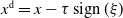 ${x}^{\text{d}}={x}-\tau \operatorname {sign}(\xi )$
is a minimizer of
${x}^{\text{d}}={x}-\tau \operatorname {sign}(\xi )$
is a minimizer of
 $\tilde {{x}}\mapsto \langle \xi ,\tilde {{x}}\rangle$
on
$\tilde {{x}}\mapsto \langle \xi ,\tilde {{x}}\rangle$
on
 $\overline {B^\infty _\tau }({x})$
. Furthermore, we define
$\overline {B^\infty _\tau }({x})$
. Furthermore, we define
 $\delta \in {\mathbb{R}}^n$
as
$\delta \in {\mathbb{R}}^n$
as
 \begin{align*} \delta _i \;:\!=\; -\operatorname {sign}({x}^{\text{d}}_i) \max \{\left |{x}^{\text{d}}_i\right | - \varepsilon , 0\}, \end{align*}
i.e., we have that
 $\mathrm{Clip}_{0,\varepsilon }({x}^{\text{d}})={x}^{\text{d}} +\delta$
. The important fact, where the choice of budget constraint matters, is that
$\mathrm{Clip}_{0,\varepsilon }({x}^{\text{d}})={x}^{\text{d}} +\delta$
. The important fact, where the choice of budget constraint matters, is that
 $\tilde {{x}} -\delta \in \overline {B_\tau ^\infty }({x})$
for all
$\tilde {{x}} -\delta \in \overline {B_\tau ^\infty }({x})$
for all
 $\tilde {{x}}\in \overline {B_\tau ^\infty }({x})\cap \overline {B_\varepsilon ^\infty }(0)$
, since we have
$\tilde {{x}}\in \overline {B_\tau ^\infty }({x})\cap \overline {B_\varepsilon ^\infty }(0)$
, since we have
 \begin{gather*} \max \{-\varepsilon , {x}_i-\tau \} \leq \tilde {{x}}_i \leq \min \{\varepsilon , {x}_i+\tau \}\\ \Rightarrow \begin{cases} \delta _i = 0&:\qquad \left |\tilde {{x}}_i -\delta _i - {x}_i\right | = \left |\tilde {{x}}_i - {x}_i\right |\leq \tau \\ \delta _i \lt 0&:\qquad {x}_i\leq \varepsilon \lt {x}_i^{\text{d}} \leq {x}_i+\tau \\ &\phantom {:}\qquad \Rightarrow \left |\tilde {{x}}_i - \delta _i-{x}_i\right | \leq \left |\varepsilon + {x}^{\text{d}}_i - \varepsilon - {x}_i\right | \leq \tau \\ \delta _i \gt 0&:\qquad \left |\tilde {{x}}_i -\delta _i - {x}_i\right | \leq \tau ,\quad \text{ analogously to the case above.} \end{cases} \end{gather*}
Now assume that there exists
 $\tilde {{x}}\in \overline {B_\varepsilon ^\infty }(0)\cap \overline {B_\tau ^\infty }({x})$
such that
$\tilde {{x}}\in \overline {B_\varepsilon ^\infty }(0)\cap \overline {B_\tau ^\infty }({x})$
such that
 $\langle \xi , \tilde {{x}}\rangle \lt \langle \xi , {x}^{\text{d}} + \delta \rangle$
. Then we infer that
$\langle \xi , \tilde {{x}}\rangle \lt \langle \xi , {x}^{\text{d}} + \delta \rangle$
. Then we infer that
 \begin{align*} \langle \xi , \tilde {{x}} - \delta \rangle \lt \langle \xi , {x}^{\text{d}} + \delta \rangle - \langle \xi , \delta \rangle = \langle \xi , {x}^{\text{d}}\rangle \end{align*}
and therefore
 ${x}^{\text{d}}$
is not a minimizer on
${x}^{\text{d}}$
is not a minimizer on
 $\overline {B_\tau ^\infty }({x})$
, which is a contradiction. Therefore, we have that
$\overline {B_\tau ^\infty }({x})$
, which is a contradiction. Therefore, we have that
 \begin{align*} {x}^{\text{d}} + \delta = \mathrm{Clip}_{0,\varepsilon }({x}^{\text{d}})= \mathrm{Clip}_{0,\varepsilon }({x} + \tau \, \operatorname {sign}(\xi )) \in \operatorname*{arg\,min} \limits_{\tilde {{x}} \in \overline {B_\tau ^\infty }({x})\cap \overline {B_\varepsilon ^\infty }(0)} \langle \xi ,\tilde {{x}}\rangle = \operatorname*{arg\,min} \limits _{\tilde {{x}} \in \overline {B_\tau ^\infty }({x})} E^{\mathrm{sl}}(\tilde {{x}};\ {x}). \end{align*}
Visualization of one (IFGSM) step, employing different norm constraints and underlying norms. The beige line marks the boundary of
 $B_\varepsilon ^p({x}^0)$
, the pink line the boundary of
$B_\varepsilon ^p({x}^0)$
, the pink line the boundary of
 $B_\tau ^q({x})$
and the intersection
$B_\tau ^q({x})$
and the intersection
 $\overline {B_\varepsilon ^p}({x}^0) \cap \overline {B_\tau ^q}({x})$
is hatched. For the case
$\overline {B_\varepsilon ^p}({x}^0) \cap \overline {B_\tau ^q}({x})$
is hatched. For the case
 $p=q=\infty$
minimizing a linear function on the intersection (blue arrow) is equivalent to first minimizing on
$p=q=\infty$
minimizing a linear function on the intersection (blue arrow) is equivalent to first minimizing on
 $\overline {B_\tau ^\infty }({x})$
(pink arrow) and then projecting back to the intersection (green arrow). This is not true for
$\overline {B_\tau ^\infty }({x})$
(pink arrow) and then projecting back to the intersection (green arrow). This is not true for
 $p=2$
. Therefore, we need to choose the appropriate projection in Lemma 5.4.
$p=2$
. Therefore, we need to choose the appropriate projection in Lemma 5.4.

This result shows that when we choose
 $p=\infty$
for the budget constraint (IFGSM) again fulfils the semi-implicit minimizing movement scheme, beyond the time restriction in Corollary 5.3.
$p=\infty$
for the budget constraint (IFGSM) again fulfils the semi-implicit minimizing movement scheme, beyond the time restriction in Corollary 5.3.
Theorem 5.5.
We consider the space
 $(\mathcal{X}, \left \|\cdot \right \|) = ({\mathbb{R}}^d, \left \|\cdot \right \|_{\infty })$
, the energy
$(\mathcal{X}, \left \|\cdot \right \|) = ({\mathbb{R}}^d, \left \|\cdot \right \|_{\infty })$
, the energy
 $E = E^{\mathrm{d}} + \chi _{\overline {B_\varepsilon ^\infty }({x}^0)}$
, with a continuously differentiable part
$E = E^{\mathrm{d}} + \chi _{\overline {B_\varepsilon ^\infty }({x}^0)}$
, with a continuously differentiable part
 $E^{\mathrm{d}}$
, which has a Lipschitz continuous gradient. Then for
$E^{\mathrm{d}}$
, which has a Lipschitz continuous gradient. Then for
 $T\gt 0$
, there exists a
$T\gt 0$
, there exists a
 $\infty$
-curve of maximal slope
$\infty$
-curve of maximal slope
 $u\;:\;[0,T]\to {\mathbb{R}}^d$
, with respect to
$u\;:\;[0,T]\to {\mathbb{R}}^d$
, with respect to
 $E$
, and a subsequence of
$E$
, and a subsequence of
 $\tau _n\;:\!=\;T/n$
such that
$\tau _n\;:\!=\;T/n$
such that
 \begin{align*} \left \|x_{\mathrm {IFGS},\tau _{n_i}}^{\lceil t/\tau _{n_i} \rceil } - u(t)\right \|\xrightarrow {i\to \infty } 0\qquad \text{ for all } t\in [0,T]. \end{align*}
Proof. Since Lemma 5.4 yields that (IFGSM) fulfils the semi-implicit minimizing movement scheme, we can proceed similarly as in the proof of Corollary 5.3. We note that all the necessary assumptions are fulfilled, since the indicator function
 $\chi _{\overline {B_\varepsilon ^\infty }({x}^0)}$
is lower semicontinuous.
$\chi _{\overline {B_\varepsilon ^\infty }({x}^0)}$
is lower semicontinuous.
5.2. Adversarial training and distributional adversaries
As before, we assume that the underlying spaces are finite dimensional, i.e.,
 $\mathcal{X}={\mathbb{R}}^d, \mathcal{Y}={\mathbb{R}}^m$
with norms
$\mathcal{X}={\mathbb{R}}^d, \mathcal{Y}={\mathbb{R}}^m$
with norms
 $\left \|\cdot \right \|_{\mathcal{X}}, \left \|\cdot \right \|_{\mathcal{Y}}$
and
$\left \|\cdot \right \|_{\mathcal{X}}, \left \|\cdot \right \|_{\mathcal{Y}}$
and
 $\mathcal{P}(\mathcal{X}\times \mathcal{Y})$
denotes the space of Borel probability measures. We consider the adversarial training task, as proposed in [Reference Goodfellow, Shlens and Szegedy46, Reference Kurakin, Goodfellow and Bengio58],
$\mathcal{P}(\mathcal{X}\times \mathcal{Y})$
denotes the space of Borel probability measures. We consider the adversarial training task, as proposed in [Reference Goodfellow, Shlens and Szegedy46, Reference Kurakin, Goodfellow and Bengio58],
 \begin{align} \inf _{h\in \mathcal{H}}\int \sup _{\tilde {{x}}\in \overline {B_\varepsilon }({x}^0)} \ell (h(\tilde {{x}}),y)\,\text{d}\mu (x,y), \end{align}
where
 $\mu \in \mathcal{P}(\mathcal{X}\times \mathcal{Y})$
denotes the data distribution and
$\mu \in \mathcal{P}(\mathcal{X}\times \mathcal{Y})$
denotes the data distribution and
 $ \ell (h(\cdot ),y) \in C^1(\mathcal{X}\times \mathcal{Y})$
. This interpretation of adversarial learning in the distributional setting has sparked a lot of interest in recent years, see e.g., [Reference Bungert, Trillos and Murray18, Reference Bungert, Trillos, Jacobs, McKenzie and Wang23, Reference Mehrabi, Javanmard, Rossi, Rao and Mai66, Reference Pydi and Jog81, Reference Pydi and Jog82, Reference Sinha, Namkoong, Volpi and Duchi96, Reference Staib and Jegelka97, Reference Zheng, Chen and Ren107]. In order to rewrite this task as a DRO problem, we equip
$ \ell (h(\cdot ),y) \in C^1(\mathcal{X}\times \mathcal{Y})$
. This interpretation of adversarial learning in the distributional setting has sparked a lot of interest in recent years, see e.g., [Reference Bungert, Trillos and Murray18, Reference Bungert, Trillos, Jacobs, McKenzie and Wang23, Reference Mehrabi, Javanmard, Rossi, Rao and Mai66, Reference Pydi and Jog81, Reference Pydi and Jog82, Reference Sinha, Namkoong, Volpi and Duchi96, Reference Staib and Jegelka97, Reference Zheng, Chen and Ren107]. In order to rewrite this task as a DRO problem, we equip
 $\mathcal{P}(\mathcal{X}\times \mathcal{Y})$
with a suitable optimal transport distance
$\mathcal{P}(\mathcal{X}\times \mathcal{Y})$
with a suitable optimal transport distance
 \begin{align*} D(\mu ,\tilde {\mu })\;:\!=\; \inf _{\gamma \in \Gamma (\mu ,\tilde {\mu } )} \gamma -\operatorname*{ess\,sup}\ c(x,y,\tilde {{x}},\tilde {y}), \end{align*}
where
 \begin{align} c(x,y,\tilde {{x}},\tilde {y})\;:\!=\; \begin{cases} \|x-\tilde {{x}}\|_{\mathcal{X}} &\text{if } y=\tilde {y},\\ +\infty &\text{if } y\neq \tilde {y}, \end{cases} \end{align}
and
 $\Gamma (\mu ,\tilde {\mu })$
denotes the set of transport plans between
$\Gamma (\mu ,\tilde {\mu })$
denotes the set of transport plans between
 $\mu$
and
$\mu$
and
 $\tilde {\mu }$
. Notably, the extended distance
$\tilde {\mu }$
. Notably, the extended distance
 $c$
is not the one naturally generated by the norms of the underlying Banach spaces
$c$
is not the one naturally generated by the norms of the underlying Banach spaces
 $\mathcal{X}$
and
$\mathcal{X}$
and
 $\mathcal{Y}$
. Nonetheless,
$\mathcal{Y}$
. Nonetheless,
 $c$
is compatible with respect to
$c$
is compatible with respect to
 $\|\cdot \|_{\mathcal{X}}+\|\cdot \|_{\mathcal{Y}}$
in the sense that
$\|\cdot \|_{\mathcal{X}}+\|\cdot \|_{\mathcal{Y}}$
in the sense that
 \begin{gather*} \liminf _{n\rightarrow \infty } c(x_n,y_n,\tilde {x}_n,\tilde {y}_n)\geq c(x,y,\tilde {x},\tilde {y}), \\ \forall (x,y),(\tilde {x},\tilde {y})\in (\mathcal{X}\times \mathcal{Y}) : (x_n,y_n)\rightarrow (y,x) , (\tilde {x}_n,\tilde {y}_n)\rightarrow (\tilde {x},\tilde {y}) \text{ w.r.t. } \|\cdot \|_{\mathcal{X}}+\|\cdot \|_{\mathcal{Y}}, \end{gather*}
compare [Reference Lisini63, Eq. (1)]. This ensures that, as we equip
 $\mathcal{P}(\mathcal{X}\times \mathcal{Y})$
with
$\mathcal{P}(\mathcal{X}\times \mathcal{Y})$
with
 $D$
, it is a well-defined extended distance, see [Reference Lisini63, section 2.6]. The cost functional
$D$
, it is a well-defined extended distance, see [Reference Lisini63, section 2.6]. The cost functional
 $c$
was similarly employed in [Reference Bui, Le, Tran, Zhao and Phung13, Reference Bungert, Trillos and Murray18]; furthermore, a similar setup was considered in [Reference Staib and Jegelka97].
$c$
was similarly employed in [Reference Bui, Le, Tran, Zhao and Phung13, Reference Bungert, Trillos and Murray18]; furthermore, a similar setup was considered in [Reference Staib and Jegelka97].
Remark 5.6. Assume that
 $\gamma \in \Gamma (\mu ,\tilde {\mu })$
is a coupling, i.e.,
$\gamma \in \Gamma (\mu ,\tilde {\mu })$
is a coupling, i.e.,
 $\gamma \in \mathcal{P}(\mathcal{Z}\times \mathcal{Z})$
, where
$\gamma \in \mathcal{P}(\mathcal{Z}\times \mathcal{Z})$
, where
 $\mathcal{Z}=\mathcal{X}\times \mathcal{Y}$
, with
$\mathcal{Z}=\mathcal{X}\times \mathcal{Y}$
, with
 $\gamma -\operatorname*{ess\,sup} c({x},y,\tilde {{x}},\tilde {y}) \lt \infty$
. Then we have that for every measurable set
$\gamma -\operatorname*{ess\,sup} c({x},y,\tilde {{x}},\tilde {y}) \lt \infty$
. Then we have that for every measurable set
 $A\subset \mathcal{Y}$
,
$A\subset \mathcal{Y}$
,
 \begin{align*} \gamma (\mathcal{X}\times A\times \mathcal{Z}) = \gamma (\mathcal{X}\times A\times \mathcal{X}\times A) = \gamma (\mathcal{Z}\times \mathcal{X}\times A), \end{align*}
which we see by contradiction: assume there exists a measurable set
 $A\subset \mathcal{Y}$
s.t., for
$A\subset \mathcal{Y}$
s.t., for
 $B\;:\!=\;\mathcal{X}\times A\times \mathcal{X}\times (\mathcal{Y}\setminus A)$
we have
$B\;:\!=\;\mathcal{X}\times A\times \mathcal{X}\times (\mathcal{Y}\setminus A)$
we have
 $\gamma (B) \gt 0$
. Then we know that
$\gamma (B) \gt 0$
. Then we know that
 $c({x},y,\tilde {{x}},\tilde {y}) = +\infty$
for all
$c({x},y,\tilde {{x}},\tilde {y}) = +\infty$
for all
 $({x},y,\tilde {{x}},\tilde {y})\in B$
and since
$({x},y,\tilde {{x}},\tilde {y})\in B$
and since
 $\gamma (B) \gt 0$
this yields that
$\gamma (B) \gt 0$
this yields that
 \begin{align*} \gamma -\operatorname*{ess\,sup} c({x},y,\tilde {{x}},\tilde {y}) \geq \gamma -\operatorname*{ess\,sup}_{B} c({x},y,\tilde {{x}},\tilde {y}) = +\infty . \end{align*}
The other identity can be proven analogously. Therefore, if
 $D(\mu ,\tilde {\mu })\lt \infty$
we know that there exists a coupling
$D(\mu ,\tilde {\mu })\lt \infty$
we know that there exists a coupling
 $\gamma$
fulfilling the above assumption and thus for every measurable set
$\gamma$
fulfilling the above assumption and thus for every measurable set
 $A\subset \mathcal{Y}$
we obtain
$A\subset \mathcal{Y}$
we obtain
 \begin{align*} \mu (\mathcal{X}\times A) = \int _{\mathcal{X}\times A \times \mathcal{Z}} \text{d}\gamma = \int _{\mathcal{Z}\times \mathcal{X}\times A} \text{d}\gamma = \tilde {\mu }(\mathcal{X}\times A). \end{align*}
If we now consider a disintegration of
 $\mu$
and
$\mu$
and
 $\tilde {\mu }$
along the
$\tilde {\mu }$
along the
 $\mathcal{X}$
-axis, i.e., we obtain
$\mathcal{X}$
-axis, i.e., we obtain
 $\,\text{d}\mu = \,\text{d}\mu _y \text{d}\nu (y), \text{d}\tilde {\mu } = \text{d}\tilde {\mu }_y \text{d}\tilde {\nu }(y)$
, with
$\,\text{d}\mu = \,\text{d}\mu _y \text{d}\nu (y), \text{d}\tilde {\mu } = \text{d}\tilde {\mu }_y \text{d}\tilde {\nu }(y)$
, with
 \begin{align*} \nu (A) = \mu ((\pi ^y)^{-1}(A)) = \mu (\mathcal{X} \times A) = \tilde {\mu }(\mathcal{X} \times A) = \tilde {\mu }((\pi ^y)^{-1}(A)) = \tilde {\nu }(A) \end{align*}
for every measurable
 $A\subset \mathcal{Y}$
, where
$A\subset \mathcal{Y}$
, where
 $\pi ^y(x,y)\;:\!=\; y$
is the projection onto the
$\pi ^y(x,y)\;:\!=\; y$
is the projection onto the
 $\mathcal{Y}$
-component.
$\mathcal{Y}$
-component.
The transport distance
 $D$
behaves like the
$D$
behaves like the
 $\infty$
-Wasserstein distance in the
$\infty$
-Wasserstein distance in the
 $\mathcal{X}$
-direction (compare section section 4) and penalizes movement of mass into the
$\mathcal{X}$
-direction (compare section section 4) and penalizes movement of mass into the
 $\mathcal{Y}$
-direction, such that no movement in
$\mathcal{Y}$
-direction, such that no movement in
 $\mathcal{Y}$
can occur when
$\mathcal{Y}$
can occur when
 $D(\mu ,\tilde {\mu })$
is finite (see Remark 5.6). Thus, all calculations done in section 4 apply with minor adaptation to this case. We only state corresponding lemmas and theorems, while adapted proofs can be found in Appendix G. The first property we prove in this section is that the adversarial training problem (5.2) is equivalent to the distributional robust optimization problem, (DRO). Note that now we need to consider a potential defined on the space
$D(\mu ,\tilde {\mu })$
is finite (see Remark 5.6). Thus, all calculations done in section 4 apply with minor adaptation to this case. We only state corresponding lemmas and theorems, while adapted proofs can be found in Appendix G. The first property we prove in this section is that the adversarial training problem (5.2) is equivalent to the distributional robust optimization problem, (DRO). Note that now we need to consider a potential defined on the space
 $\mathcal{X}\times \mathcal{Y}$
, namely
$\mathcal{X}\times \mathcal{Y}$
, namely
 $E({x},y)\;:\!=\;-\ell (h({x}), y)$
, where the label
$E({x},y)\;:\!=\;-\ell (h({x}), y)$
, where the label
 $y$
is now also a variable argument.
$y$
is now also a variable argument.
Corollary 5.7. It holds that
 \begin{align} \int \max _{\tilde {{x}}\in \overline {B_\varepsilon }(\tilde {{x}})} \ell (h({x}),y) \,\text{d}\mu (x,y)= \max _{\tilde {\mu }\;:\;D(\tilde {\mu },\mu )\leq \varepsilon }\int \ell (h({x}),y) d \tilde {\mu }({x},y) \end{align}
where the maximizing argument is given by
 $\mu _{\max }=(r_\varepsilon )_{\#}\mu$
, with
$\mu _{\max }=(r_\varepsilon )_{\#}\mu$
, with
 $r_\varepsilon \;:\;\mathcal{X}\times \mathcal{Y}\to \mathcal{X}$
being a
$r_\varepsilon \;:\;\mathcal{X}\times \mathcal{Y}\to \mathcal{X}$
being a
 $\mathcal{B}(\mathcal{X}\times \mathcal{Y})$
-measurable selector from Lemma G.1
$\mathcal{B}(\mathcal{X}\times \mathcal{Y})$
-measurable selector from Lemma G.1
Proof. We employ the
 $\mathcal{B}(\mathcal{X}\times \mathcal{Y})$
-measurable selector
$\mathcal{B}(\mathcal{X}\times \mathcal{Y})$
-measurable selector
 $r_\varepsilon$
, from Lemma G.1 and compute
$r_\varepsilon$
, from Lemma G.1 and compute
 \begin{align*} \int \max _{\tilde {{x}}\in \overline {B_\varepsilon }({x})} \ell (h(\tilde {{x}}),y)\, \,\text{d}\mu ({x},y) &=\int \max _{(\tilde {{x}}, \tilde {y}): c({x},y,\tilde {{x}},\tilde {y}) \leq \varepsilon } -{E}(\tilde {{x}},\tilde {y})\, \,\text{d}\mu ({x},y) =\int -{E}(r_\varepsilon (x,y))\, \,\text{d}\mu ({x},y)\\ &=-\int {E}(x,y) d(r_{\varepsilon })_\#\mu ({x}, y)\overset {(i)}{=} -\min _{\tilde {\mu }\;:\;D(\mu ,\tilde {\mu })\leq \varepsilon } \int {E}(x,y)\, d\tilde {\mu }({x},y)\\ &=\max _{\tilde {\mu }\;:\;D(\tilde {\mu },\mu )\leq \varepsilon }\int \ell (h({x}),y) d \tilde {\mu }({x},y), \end{align*}
where in
 $(i)$
we employ (G.1).
$(i)$
we employ (G.1).
Remark 5.8. In other works considering distributional adversarial attacks, for example [Reference Pydi and Jog81, Reference Pydi and Jog82], the well-definedness of the expressions in Corollary 5.7 is not always ensured. In [Reference Bungert, Trillos and Murray18], this was resolved by considering open balls for the budget constraint. However, due to our assumption that
 $\ell (h(\cdot ), y)\in C^1(\mathcal{X}\times \mathcal{Y})$
, we do not encounter similar measurability issues, as shown in [Reference Meunier, Scetbon, Pinot, Atif and Chevaleyre67].
$\ell (h(\cdot ), y)\in C^1(\mathcal{X}\times \mathcal{Y})$
, we do not encounter similar measurability issues, as shown in [Reference Meunier, Scetbon, Pinot, Atif and Chevaleyre67].
For the main result in this section, we now consider the energy defined via the potential defined on
 $\mathcal{X}\times \mathcal{Y}$
, i.e.,
$\mathcal{X}\times \mathcal{Y}$
, i.e.,
 \begin{align*} \mathcal{E}(\mu )\;:\!=\;\int {E}({x},y) \,\text{d}\mu ({x},y) = \int -\ell (h(x),y) \,\text{d}\mu (x,y), \end{align*}
where the underlying extended metric space is chosen as
 $\mathcal{D}=(\mathcal{P}_\infty (\mathcal{X}\times \mathcal{Y}), c)$
, with
$\mathcal{D}=(\mathcal{P}_\infty (\mathcal{X}\times \mathcal{Y}), c)$
, with
 $\mathcal{P}_\infty (\mathcal{X}\times \mathcal{Y})$
denoting the subset of Borel probability measures with bounded support in
$\mathcal{P}_\infty (\mathcal{X}\times \mathcal{Y})$
denoting the subset of Borel probability measures with bounded support in
 $\mathcal{X}$
- and
$\mathcal{X}$
- and
 $\mathcal{Y}$
-direction.
$\mathcal{Y}$
-direction.
Remark 5.9. Theorem 4.7 also holds for extended distances, i.e., distances which take values in
 $[0,+\infty ]$
, compare [Reference Lisini63, Theorem 3.1]. The distance
$[0,+\infty ]$
, compare [Reference Lisini63, Theorem 3.1]. The distance
 $c(\cdot ,\cdot )$
introduced in (5.3) is such an extended distance. For this particular choice of extended distance, the measure
$c(\cdot ,\cdot )$
introduced in (5.3) is such an extended distance. For this particular choice of extended distance, the measure
 \begin{equation*}\eta \in \mathcal{P} \left(C (0,T;\ ((\mathcal{X}\times \mathcal{Y}),\|\cdot \|_{\mathcal{X}}+\|\cdot \|_{\mathcal{Y}}) \right)\end{equation*}
is concentrated on
 $AC^\infty \left (0,T;\left ((\mathcal{X}\times \mathcal{Y}),c\right )\right )=AC^\infty (0,T;\;(\mathcal{X},\|\cdot \|_{\mathcal{X}})\times \mathcal{Y})$
. Notice that the continuous curves are continuous w.r.t.
$AC^\infty \left (0,T;\left ((\mathcal{X}\times \mathcal{Y}),c\right )\right )=AC^\infty (0,T;\;(\mathcal{X},\|\cdot \|_{\mathcal{X}})\times \mathcal{Y})$
. Notice that the continuous curves are continuous w.r.t.
 $\|\cdot \|_{\mathcal{X}}+\|\cdot \|_{\mathcal{Y}}$
, while absolute continuity is w.r.t.
$\|\cdot \|_{\mathcal{X}}+\|\cdot \|_{\mathcal{Y}}$
, while absolute continuity is w.r.t.
 $c(\cdot ,\cdot )$
(compare [Reference Lisini63, section 2.3.]).
$c(\cdot ,\cdot )$
(compare [Reference Lisini63, section 2.3.]).
The theorem below is a variant of Theorem 4.18 for the adversarial setting. Namely, we show that
 $\infty$
-curves of maximal slope that are used to solve (DRO) can be characterized by employing a representing measure
$\infty$
-curves of maximal slope that are used to solve (DRO) can be characterized by employing a representing measure
 $\eta$
on
$\eta$
on
 $C(0,T;\;\mathcal{X}\times \mathcal{Y})$
, where
$C(0,T;\;\mathcal{X}\times \mathcal{Y})$
, where
 $\eta$
-a.e. curve fulfils the differential inclusion w.r.t. the potential
$\eta$
-a.e. curve fulfils the differential inclusion w.r.t. the potential
 $E$
. Here, we enforce the condition
$E$
. Here, we enforce the condition
 $D(\mu ,\tilde {\mu })\leq \varepsilon$
, by only considering the evolution until time
$D(\mu ,\tilde {\mu })\leq \varepsilon$
, by only considering the evolution until time
 $T=\epsilon$
.
$T=\epsilon$
.
Theorem 5.10.
For
 $T=\varepsilon$
, let
$T=\varepsilon$
, let
 $\mu \in {\mathrm{AC}}^\infty (0,T;\ \mathcal{D})$
with
$\mu \in {\mathrm{AC}}^\infty (0,T;\ \mathcal{D})$
with
 $\eta$
from Theorem 4.7
. Let further
$\eta$
from Theorem 4.7
. Let further
 $ \mathcal{E} \circ \mu$
be for a.e.
$ \mathcal{E} \circ \mu$
be for a.e.
 $t\in [0,T]$
equal to a non-increasing map
$t\in [0,T]$
equal to a non-increasing map
 $\psi \;:\;[0,T] \rightarrow {\mathbb{R}}$
.
$\psi \;:\;[0,T] \rightarrow {\mathbb{R}}$
.
Then the following statements are equivalent:
-
(i)
$ |\mu '|(t)\leq 1 \text{ and } \psi '(t)\leq -|\partial \mathcal{E}|(u(t)) \text{ for a.e. } t\in (0,T).$
-
(ii) For
$\eta$
-a.e. curve
$u\in C(0,T;\;\mathcal{X}\times \mathcal{Y})$
it holds, that
$E\circ u$
is for a.e.
$t\in (0,T)$
equal to a non-increasing map
$\psi _u: [0,T]\rightarrow {\mathbb{R}}$
and
\begin{equation*} u'(t)\ \in \ (\partial \|\cdot \|_{\mathcal{X}^*}({-}\nabla _x E(u(t))),0) , \quad \text{for a.e. } t\in (0,T).\end{equation*}


Proof. Step 1:
 $(\text{i})\Longrightarrow (\text{ii})$
.
$(\text{i})\Longrightarrow (\text{ii})$
.
By Lemma G.2, we know that
 $|\partial \mathcal{E} |$
is a strong upper gradient such that by Remark 2.3
$|\partial \mathcal{E} |$
is a strong upper gradient such that by Remark 2.3
 $\mu _t$
satisfies the energy dissipation equality (2.10). Similar to Theorem 4.18, we estimate
$\mu _t$
satisfies the energy dissipation equality (2.10). Similar to Theorem 4.18, we estimate
 \begin{align} \begin{split}\mathcal{E} (\mu _0)- \mathcal{E} (\mu _T)&= \int _{C(0,T;\;\mathcal{X})} E(u(0))-E(u(T)) \,\text{d}\eta (u)\\ &\leq \int _{C(0,T;\;\mathcal{X})} \int _0^T \|\nabla _x E(u(r))\|_{\mathcal{X}^*} |u'|(t) \,\text{d}r \,\text{d}\eta (u)\\ &\leq \int _{C(0,T;\;\mathcal{X})} \int _0^T \|\nabla _x E(u(r))\|_{\mathcal{X}^*} \,\text{d}r \,\text{d}\eta (u)\\ &=\int _0^T |\partial \mathcal{E}|(\mu (r))\,\text{d}r=\mathcal{E}(\mu _0)-\mathcal{E}(\mu _T). \end{split} \end{align}
and observe that this equality can only hold if for
 $\eta$
.a.e.
$\eta$
.a.e.
 $u$
$u$
 \begin{align*} E(u(s))-E(u(t))= \int _s^t \|\nabla _x E(u(r))\|_{\mathcal{X}^*} |u'|(t) \,\text{d}r = \int _s^t \|\nabla _x E(u(r))\|_{\mathcal{X}^*} \,\text{d}r \quad \text{ for all } 0 \leq s \lt t \leq T. \end{align*}
and thus
 $\psi _u \;:\!=\; E\circ u$
is a non-increasing absolutely continuous map for
$\psi _u \;:\!=\; E\circ u$
is a non-increasing absolutely continuous map for
 $\eta$
-a.e.
$\eta$
-a.e.
 $u$
.
$u$
.
We use Lemma E.4 and
 $\||u'|(t)\|_{L^\infty (\eta )}=|\mu '|(t)\leq 1$
for a.e.
$\||u'|(t)\|_{L^\infty (\eta )}=|\mu '|(t)\leq 1$
for a.e.
 $t\in (0,T)$
to infer that for
$t\in (0,T)$
to infer that for
 $\eta$
-a.e. curve
$\eta$
-a.e. curve
 $u\in C(0,T;\;\mathcal{X}\times \mathcal{Y})$
it holds,
$u\in C(0,T;\;\mathcal{X}\times \mathcal{Y})$
it holds,
 \begin{equation*} \left |u'\right |(t)\leq 1 \quad \text{for a.e. } t\in (0,T).\end{equation*}
Denoting by
 $(u'(t))_x$
and
$(u'(t))_x$
and
 $(u'(t))_y$
the
$(u'(t))_y$
the
 $\mathcal{X}$
and
$\mathcal{X}$
and
 $\mathcal{Y}$
corresponding parts of the derivative
$\mathcal{Y}$
corresponding parts of the derivative
 $u'(t)$
and keeping Lemma 3.7 in mind we obtain for
$u'(t)$
and keeping Lemma 3.7 in mind we obtain for
 $\eta$
-a.e. curve
$\eta$
-a.e. curve
 $u\in C(0,T;\;\mathcal{X}\times \mathcal{Y})$
 \begin{align*} \langle \nabla _x E(x,y),(u'(t))_x\rangle &=\langle \nabla E(x,y), u'(t)\rangle \\ &= ({E}\circ u)'(t) \\ &= -\|\nabla _x E(u(r))\|_{\mathcal{X}^*} =-\left \|\nabla _x E(u(r))\right \|_{\mathcal{X}^*}-\chi _{\overline {B_1}}((u'(t))_x) \end{align*}
for a.e.
 $t\in (0,T)$
. Using the equivalence of Item 3 and Item 1 we obtain
$t\in (0,T)$
. Using the equivalence of Item 3 and Item 1 we obtain
 \begin{align*} u'(t)\ \in \ (\partial \|\cdot \|_{\mathcal{X}^*}({-}\nabla _x E(x,y)),0) \quad \text{for a.e. } t\in (0,T) \end{align*}
for
 $\eta$
-a.e. curve
$\eta$
-a.e. curve
 $u$
.
$u$
.
Step 2:
 $(\text{ii})\Longrightarrow (\text{i})$
.
$(\text{ii})\Longrightarrow (\text{i})$
.
For
 $\eta$
-a.e.
$\eta$
-a.e.
 $u\in C(0,T;\;\mathcal{X} \times \mathcal{Y})$
we know by Remark 2.3 that the energy dissipation equality
$u\in C(0,T;\;\mathcal{X} \times \mathcal{Y})$
we know by Remark 2.3 that the energy dissipation equality
 \begin{align*} E(u(s))-E(u(t)) = \int _s^t \|\nabla _x E(u(r))\|_{\mathcal{X}^*} \,\text{d}r \quad \text{ for all } 0 \leq s \lt t \leq T. \end{align*}
holds. In particular, it is absolutely continuous such that Remark 1.3 applies. We calculate,
 \begin{align*} \mathcal{E} (\mu _t) &- \mathcal{E} (\mu _s) = \int _{C(0,T; \mathcal{X})} E(u(t))-E(u(s)) \,\text{d}\eta (u) = \int _{C(0,T ; \mathcal{X})} \int _s^t (E\circ u)'(r) \,\text{d}r \,\text{d}\eta (u)\\ &= \int _{C(0,T ; \mathcal{X})} \int _s^t \langle \nabla _x E(u(r)),(u'(r))_x\rangle \,\text{d}r \,\text{d}\eta (u)\overset {(i)}{=}\int _{C(0,T ; \mathcal{X})} \int _s^t -\|\nabla _xE(u(r))\|_{\mathcal{X}^*} \,\text{d}r \,\text{d}\eta (u)\\ &=\int _{C(0,T ; \mathcal{X})} \int _s^t -\|\nabla _xE(u(r))\|_{\mathcal{X}^*} \,\text{d}\eta (u)\,\text{d}r\overset {(ii)}{=}\int _s^t -|\partial \mathcal{E} |(\mu _r) \,\text{d}r, \end{align*}
Where for (i) we use the equivalence of Item 3 and Item 1, while for (ii) we use Lemma G.2. This implies
 $\mathcal{E} \circ \mu _t$
is monotone non-increasing and
$\mathcal{E} \circ \mu _t$
is monotone non-increasing and
 $(\mathcal{E} \circ \mu )'(t)\leq -|\partial \mathcal{E}|(\mu _t)$
for a.e.
$(\mathcal{E} \circ \mu )'(t)\leq -|\partial \mathcal{E}|(\mu _t)$
for a.e.
 $t\in (0,T)$
. Further, by Theorem 4.7, we have
$t\in (0,T)$
. Further, by Theorem 4.7, we have
 \begin{align*} |\mu '|(t)=\eta (u)-\operatorname*{ess\,sup} |u'|(t) =\eta (u)-\operatorname*{ess\,sup} \|u'(t)\|_{\mathcal{X}} \leq 1, \end{align*}
since all elements in
 $\partial \|\cdot \|_{\mathcal{X}^*}({-}\nabla _x E(x,y))$
have norm smaller than
$\partial \|\cdot \|_{\mathcal{X}^*}({-}\nabla _x E(x,y))$
have norm smaller than
 $1$
.
$1$
.
6. Conclusion and outlook
In this work, we considered the limit case
 $p\to \infty$
of the well-known
$p\to \infty$
of the well-known
 $p$
-curves of maximum slope, which yield a versatile gradient flow framework in metric spaces, [Reference Ambrosio, Gigli and Savaré2]. In the abstract setting, we proved existence by employing the minimizing movement scheme, adapted to the case
$p$
-curves of maximum slope, which yield a versatile gradient flow framework in metric spaces, [Reference Ambrosio, Gigli and Savaré2]. In the abstract setting, we proved existence by employing the minimizing movement scheme, adapted to the case
 $p=\infty$
. Assuming that the underlying space is Banach, we were able to characterize
$p=\infty$
. Assuming that the underlying space is Banach, we were able to characterize
 $\infty$
-curves of maximum slope via differential inclusions. Furthermore, we also demonstrated the convergence of a semi-implicit scheme to the continuum flow. This insight constitutes the interface to the field of adversarial attacks. Namely, we showed that the well-known FGSM, and its iterative variant, correspond to the semi-implicit scheme and therefore converge to the flow, when sending the step size to zero. More generally, this result holds true for a whole class of normalized gradient descent algorithms. Furthermore, we also considered Wasserstein gradient flows, where we first used the theory developed in [Reference Lisini63] to derive an alternative characterization of absolutely continuous curves via the continuity equation. As our main result in this section, we prove that being an
$\infty$
-curves of maximum slope via differential inclusions. Furthermore, we also demonstrated the convergence of a semi-implicit scheme to the continuum flow. This insight constitutes the interface to the field of adversarial attacks. Namely, we showed that the well-known FGSM, and its iterative variant, correspond to the semi-implicit scheme and therefore converge to the flow, when sending the step size to zero. More generally, this result holds true for a whole class of normalized gradient descent algorithms. Furthermore, we also considered Wasserstein gradient flows, where we first used the theory developed in [Reference Lisini63] to derive an alternative characterization of absolutely continuous curves via the continuity equation. As our main result in this section, we prove that being an
 $\infty$
-curve of maximal slope is equivalent to the existence of a representing measure on the space of continuous curves, where almost every curve, fulfils a differential inclusion on the underlying Banach space. This finally allowed us to generate distributional adversaries, in an adapted
$\infty$
-curve of maximal slope is equivalent to the existence of a representing measure on the space of continuous curves, where almost every curve, fulfils a differential inclusion on the underlying Banach space. This finally allowed us to generate distributional adversaries, in an adapted
 $\infty$
-Wasserstein distance, via curves of maximum slope. Similar to section 5, we could also consider the energy
$\infty$
-Wasserstein distance, via curves of maximum slope. Similar to section 5, we could also consider the energy
 \begin{align*} \mathcal{E}(\mu )\;:\!=\;\int _{\mathcal{X}\times \mathcal{Y}} E(x,y) \,\text{d}\mu +\chi _{B^D_\epsilon (\mu _0)}(\mu ) \end{align*}
to generate distributional adversarial attacks. We strongly suspect that corresponding
 $\infty$
-curves of maximal slope in
$\infty$
-curves of maximal slope in
 $\mathcal{D}$
would take the following form: Let
$\mathcal{D}$
would take the following form: Let
 $\mu \in AC^\infty (0,T;\;\mathcal{X})$
be a
$\mu \in AC^\infty (0,T;\;\mathcal{X})$
be a
 $\infty$
-curve of maximal slope and
$\infty$
-curve of maximal slope and
 $\eta$
its corresponding probability measure over the space
$\eta$
its corresponding probability measure over the space
 $C(0,T;\;\mathcal{X}\times \mathcal{Y})$
, then for
$C(0,T;\;\mathcal{X}\times \mathcal{Y})$
, then for
 $\eta$
-a.e.
$\eta$
-a.e.
 $u\in C(0,T;\;\mathcal{X}\times \mathcal{Y})$
 \begin{align*} u'(t)\ \in \ (\partial \|\cdot \|_{\mathcal{X}^*}({-}\nabla _x E_{u_0}(u(t))),0) , \quad \text{for a.e. } t\in (0,T), \end{align*}
where
 \begin{align*} E_{u_0}(x,y)=E(x,y)+\chi _{B_\epsilon ((u_0)_x)}(x). \end{align*}
In [Reference Wong, Rice and Kolter105], the authors suggested to combine FGSM with stochastic elements. They proposed to use a single step
 \begin{gather*} \sigma \sim \text{Uniform}\left (\overline {B_\epsilon ^\infty }(x_0)\right ),\\ x_\frac {1}{2}=x_0+\sigma ,\\ x_1=\mathrm{Clip}_{0,\varepsilon }\left (x_\frac {1}{2}+\operatorname {sign}(\nabla \ell (h(x_\frac {1}{2}), y))\right ). \end{gather*}
This is reminiscent of the classical Langevin algorithm, therefore, it would be interesting if this stochasticity could be incorporated into our framework.
Acknowledgements
MB, TR and LW acknowledge support from DESY (Hamburg, Germany), a member of the Helmholtz Association HGF. This research was supported in part through the Maxwell computational resources operated at Deutsches Elektronen-Synchrotron DESY, Hamburg, Germany. TR further wants to thank Samira Kabri for many insightful discussions. Parts of this study were carried out while LW and TR were affiliated with the Friedrich-Alexander-Universität Erlangen-Nürnberg.
Financial support
MB and TR acknowledge funding by the German Ministry of Science and Technology (BMBF) under grant agreement No. 01IS24072A (COMFORT). MB and LW acknowledge funding from the German Research Foundation, project BU 2327/20-1.
Competing interests
The authors declare none.
Appendix
A Convex analysis
This section gives an overview over well-known definitions and statements in convex analysis. In the following,
 $\mathcal{X}$
denotes a Banach space and
$\mathcal{X}$
denotes a Banach space and
 $\mathcal{X}^*$
its dual.
$\mathcal{X}^*$
its dual.
Definition A.1 (Subdifferential). For a convex function
 $f\;:\;\mathcal{X}\to ({-}\infty , \infty ]$
, we denote by
$f\;:\;\mathcal{X}\to ({-}\infty , \infty ]$
, we denote by
 \begin{align*} \partial f({x}) \;:\!=\; \{\xi \in \mathcal{X}^*\;:\ f(z) - f({x}) \geq \langle \xi , z - {x} \rangle \quad \forall z\in \mathcal{X}\} \subset \mathcal{X}^* \end{align*}
the subdifferential of
 $f$
at
$f$
at
 $x\in \mathcal{X}$
.
$x\in \mathcal{X}$
.
If
 $f(\cdot )=\|\cdot \|$
, then the subdifferential is given by
$f(\cdot )=\|\cdot \|$
, then the subdifferential is given by
 \begin{align} \partial \|\cdot \|(x)= \left\{ \xi \in \mathcal{X}^*|\langle \xi , x\rangle =\|x\|,\|\xi \|_*\leq 1 \right\} \end{align}
Definition A.2 (Fenchel conjugate). For a function
 $f\;:\;\mathcal{X} \rightarrow [-\infty ,+\infty ]$
, we denote by
$f\;:\;\mathcal{X} \rightarrow [-\infty ,+\infty ]$
, we denote by
 $f^*: \mathcal{X}^* \rightarrow [{-}\infty ,+\infty ]$
,
$f^*: \mathcal{X}^* \rightarrow [{-}\infty ,+\infty ]$
,
 \begin{align*} f^*(\xi )\;:\!=\; \sup _{x\in \mathcal{X}} \langle \xi , {x}\rangle -f({x}) \quad \text{for } \xi \in \mathcal{X}^* \end{align*}
the Fenchel conjugate of
 $f$
.
$f$
.
A direct consequence of this definition is the so called Fenchel–Young inequality
 \begin{align} \langle \xi ,{x}\rangle \leq f({x})+f^*(\xi ). \end{align}
The next proposition yields the conditions under which the equality in (A.2) is obtained.
Proposition A.3 [Reference Barbu and Precupanu6, Proposition 2.33]. Let
 $f\;:\;\mathcal{X}\rightarrow ]-\infty ,+\infty ]$
be a proper convex function. Then for
$f\;:\;\mathcal{X}\rightarrow ]-\infty ,+\infty ]$
be a proper convex function. Then for
 $x\in \mathcal{X}$
, the following three properties are equivalent:
$x\in \mathcal{X}$
, the following three properties are equivalent:
-
(i)
$\xi \in \partial f(x)$
. -
(ii)
$f(x)+f^*(\xi )\leq \langle \xi ,x\rangle$
. -
(iii)
$f(x)+f^*(\xi )=\langle \xi ,x\rangle$
.

If, in addition,
 $f$
is lower-semicontinuous, then all of these properties are equivalent to the following one.
$f$
is lower-semicontinuous, then all of these properties are equivalent to the following one.
-
(i)
$x\in \partial f^*(\xi )$
.

Remark A.4. In Item 1, we use the canonical embedding to obtain the subspace relation
 $\mathcal{X}\subset \mathcal{X}^{**}$
. Following [Reference Barbu and Precupanu6, Remark 2.35], if
$\mathcal{X}\subset \mathcal{X}^{**}$
. Following [Reference Barbu and Precupanu6, Remark 2.35], if
 $\mathcal{X}$
is reflexive, i.e.
$\mathcal{X}$
is reflexive, i.e.
 $\mathcal{X}^{**}=\mathcal{X}$
, then it follows from Proposition A.3 that
$\mathcal{X}^{**}=\mathcal{X}$
, then it follows from Proposition A.3 that
 \begin{align*} x\in \partial f^*(\xi ) \Longleftrightarrow \xi \in \partial f(x), \end{align*}
which yields
 \begin{align*} (\partial f)^{-1}(\xi ) = \{x\in \mathcal{X}\,:\, \xi \in \partial f(x)\} = \{x\in \mathcal{X}\,:\, x\in \partial f^*(\xi )\} = \partial f^*(\xi ) \end{align*}
In the non-reflexive case, one can not argue as above, and we do not obtain the simple relation between
 $\partial f^*$
and
$\partial f^*$
and
 $\partial f$
, see, e.g., [84].
$\partial f$
, see, e.g., [84].
An important corollary of Proposition A.3 is its application to the indicator function of the closed unit ball
 $f=\chi _{\overline {B_1}}$
, where its convex conjugate for
$f=\chi _{\overline {B_1}}$
, where its convex conjugate for
 $\xi \in \mathcal{X}^*$
is given by
$\xi \in \mathcal{X}^*$
is given by
 \begin{align*} \chi _{\overline {B_1}}^*(\xi )= \sup _{{x}\in \mathcal{X}}\langle \xi , {x}\rangle -\chi _{\overline {B_1}}({x})= \sup _{{x}\in \overline {B_1}}\langle \xi , {x}\rangle =\|\xi \|_*. \end{align*}
Corollary A.5.
For a Banach space
 $\mathcal{X}$
, and
$\mathcal{X}$
, and
 $\xi \in \mathcal{X}^*$
we have that
$\xi \in \mathcal{X}^*$
we have that
 \begin{align} \partial \left \|\cdot \right \|_*(\xi )\cap \mathcal{X} = \operatorname*{arg\,max}_{{x}\in \overline {B_1}} \langle \xi , {x}\rangle . \end{align}
Proof. Since
 $\chi _{\overline {B_1}}$
is lower semicontinuous, we can use the equivalence of Item 3 and Item 1, to infer
$\chi _{\overline {B_1}}$
is lower semicontinuous, we can use the equivalence of Item 3 and Item 1, to infer
 \begin{align*} {x}\in \partial \left \|\cdot \right \|_*(\xi ) \quad \Leftrightarrow \quad \left \|\xi \right \|_* = \langle \xi ,{x}\rangle - \chi _{\overline {B_1}}({x}). \end{align*}
In the second statement, using the definition of
 $\left \|\xi \right \|_*$
as in (A.3), therefore yields that each
$\left \|\xi \right \|_*$
as in (A.3), therefore yields that each
 $x$
above realizes the supremum, which concludes the proof.
$x$
above realizes the supremum, which concludes the proof.
B Refined version of Ascoli–Arzelà
Proposition B.1 [Reference Ambrosio, Gigli and Savaré2, Proposition 3.3.1]. Let
 $u^n\;:\;[0,T]\to \mathcal{S}$
be a sequence of curves, that fulfils the following conditions:
$u^n\;:\;[0,T]\to \mathcal{S}$
be a sequence of curves, that fulfils the following conditions:
-
(AA-i) There is a
$\sigma$
-sequentially compact set
$K\subset \mathcal{S}$
, such that
\begin{align*} u^n(t)\in K\quad \text{for every}\quad t\in [0,T]\quad \text{and every}\quad n\in \mathbb{N}. \end{align*}
-
(AA-ii) There is a symmetric function
$\omega \;:\;[0,T]\times [0,T]\to [0,+\infty )$
with
$\lim _{(s,t)\to (r,r)} \omega (s,t) = 0$
for all
$r\in [0,T]\setminus C$
, where
$C$
is an at most countable set, such that
\begin{align*} \limsup _{n\to \infty } d(u^n(s), u^n(t))\leq \omega (s,t)\quad \text{for all}\quad s,t\in [0,T]. \end{align*}


Then there exists a subsequence
 $u^{n_k}$
and a limit curve
$u^{n_k}$
and a limit curve
 $u\;:\;[0,T]\to \mathcal{S}$
, which is
$u\;:\;[0,T]\to \mathcal{S}$
, which is
 $d$
-continuous in
$d$
-continuous in
 $[0,T]\setminus C$
, such that
$[0,T]\setminus C$
, such that
 \begin{align*} u^{n_k}(t) \overset {\sigma }{\rightharpoonup } u(t)\quad \text{for all}\quad t\in [0,T]. \end{align*}
C Taylor’s formula in Banach spaces
Theorem C.1.
Suppose
 $E$
,
$E$
,
 $F$
are real Banach spaces,
$F$
are real Banach spaces,
 $U\subset E$
an open and nonempty subset, and
$U\subset E$
an open and nonempty subset, and
 $f\in C^n(U,F)$
. Given
$f\in C^n(U,F)$
. Given
 $x_0\in U$
choose
$x_0\in U$
choose
 $r\gt 0$
such that
$r\gt 0$
such that
 $x_0+B_r \subset U$
, where
$x_0+B_r \subset U$
, where
 $B_r$
is the open ball in
$B_r$
is the open ball in
 $E$
with centre
$E$
with centre
 $0$
and radius
$0$
and radius
 $r$
. Then for all
$r$
. Then for all
 $h\in B_r$
we have, using the abbreviation
$h\in B_r$
we have, using the abbreviation
 $h^k=(h,\ldots ,h)$
,
$h^k=(h,\ldots ,h)$
,
 $k$
terms,
$k$
terms,
 \begin{align*} f(x_0 +h)=\sum _{k=0}^n \frac {1}{k!} f(k) (x_0)(h)^k +R_n(x_0,h), \end{align*}
where the remainder
 $R_n$
is of form
$R_n$
is of form
 \begin{align*} R_n(x_0,h)= \frac {1}{(n-1)!} \int _0^1 (1-t)^{n-1} [f^{(n)}(x_0+th)-f^{(n)}(x_0)] (h)^n \,\text{d}t. \end{align*}
Proof. A proof for this statement can be found, e.g., in [Reference Blanchard and Brüning8, Theorem 30.1.3].
D Prokhorov’s theorem
Theorem D.1 (Prokhorov [Reference Billingsley7, Theorems 5.1–5.2]). If a set
 $\mathcal{K}\subset \mathcal{P}(\mathcal{X})$
is tight, i.e.,
$\mathcal{K}\subset \mathcal{P}(\mathcal{X})$
is tight, i.e.,
 \begin{align} \forall \epsilon \gt 0\quad \exists K_\epsilon \text{ compact in } \mathcal{X} \text{ such that } \mu (\mathcal{X}\setminus K_\epsilon )\leq \epsilon \quad \forall \mu \in \mathcal{K}, \end{align}
then
 $\mathcal{K}$
is relatively compact in
$\mathcal{K}$
is relatively compact in
 $\mathcal{P}(\mathcal{X})$
. Conversely, if
$\mathcal{P}(\mathcal{X})$
. Conversely, if
 $\mathcal{X}$
is a Polish space, every relatively compact subset of
$\mathcal{X}$
is a Polish space, every relatively compact subset of
 $\mathcal{P}(\mathcal{X})$
is tight.
$\mathcal{P}(\mathcal{X})$
is tight.
E Helpful lemmas and supplementary proofs
In the following, we provide the proof of Lemma 2.8, which is a particular case of [Reference Ambrosio, Gigli and Savaré2, Lemma 3.1.5]. For completeness, we provide a version of the proof that is specifically adapted to the case
 $p=\infty$
.
$p=\infty$
.
Proof of Lemma
2.8. Let us suppose that for all
 $\tau \gt 0$
,
$\tau \gt 0$
,
 $\mathcal{E}_\tau ({x})\lt \mathcal{E}({x})$
else
$\mathcal{E}_\tau ({x})\lt \mathcal{E}({x})$
else
 $|\partial \mathcal{E}|({x})=0$
and equality (2.4) holds trivially. We calculate
$|\partial \mathcal{E}|({x})=0$
and equality (2.4) holds trivially. We calculate
 \begin{align*} \limsup _{\tau \rightarrow 0^+} \frac {\mathcal{E}({x})-\mathcal{E}_\tau ({x})}{\tau } &= \limsup _{\tau \rightarrow 0^+}\sup _{z:0\lt d({x},z)\leq \tau } \frac {\mathcal{E}({x})-\mathcal{E}(z)}{\tau }\\ &= \inf _{\epsilon \gt 0} \sup _{0\lt \tau \leq \epsilon } \sup _{z:0\lt d({x},z)\leq \tau } \frac {\mathcal{E}({x})-\mathcal{E}(z)}{\tau }\\ &= \inf _{\epsilon \gt 0} \sup _{z,\tau :0\lt d({x},z)\leq \tau \leq \epsilon } \frac {\mathcal{E}({x})-\mathcal{E}(z)}{\tau }\\ &=\inf _{\epsilon \gt 0} \sup _{z:0\lt d({x},z)\leq \epsilon } \sup _{\tau :d({x},z)\leq \tau \leq \epsilon } \frac {\mathcal{E}({x})-\mathcal{E}(z)}{\tau }\\ & =\inf _{\epsilon \gt 0} \sup _{z:0\lt d({x},z)\leq \epsilon } \frac {(\mathcal{E}(x)-\mathcal{E}(z))^+}{d(x,z)}-\frac {(\mathcal{E}(x)-\mathcal{E}(z))^-}{\epsilon } \\ &\stackrel {(*)}{=}\inf _{\epsilon \gt 0} \sup _{z:0\lt d({x},z) \leq \epsilon } \frac {\mathcal{E}({x})-\mathcal{E}(z)}{d({x},z)}\\ &=\limsup _{z \rightarrow {x}} \frac {\mathcal{E}({x})-\mathcal{E}(z)}{d({x},z)}\\ &= |\partial \mathcal{E}|({x}). \end{align*}
Equality
 $(*)$
can be verified by the observation that
$(*)$
can be verified by the observation that
 $\mathcal{E}_\tau ({x})\lt \mathcal{E}({x})$
for all
$\mathcal{E}_\tau ({x})\lt \mathcal{E}({x})$
for all
 $\tau \gt 0$
ensures the existence of at least one
$\tau \gt 0$
ensures the existence of at least one
 $z$
with
$z$
with
 $d({x},z)\leq \epsilon$
such that
$d({x},z)\leq \epsilon$
such that
 $\mathcal{E}({x})-\mathcal{E}(z)\geq 0$
.
$\mathcal{E}({x})-\mathcal{E}(z)\geq 0$
.
Lemma E.1.
Let
 $\phi \;:\;[0,T]\rightarrow {\mathbb{R}}$
be continuous and
$\phi \;:\;[0,T]\rightarrow {\mathbb{R}}$
be continuous and
 $\psi \;:\;[0,T]\rightarrow {\mathbb{R}}$
be non-increasing. If
$\psi \;:\;[0,T]\rightarrow {\mathbb{R}}$
be non-increasing. If
 $\phi (t)=\psi (t)$
for a.e.
$\phi (t)=\psi (t)$
for a.e.
 $t\in [0,T]$
, then
$t\in [0,T]$
, then
 $\phi (t)=\psi (t)$
for all
$\phi (t)=\psi (t)$
for all
 $t\in (0,T)$
.
$t\in (0,T)$
.
Proof. Assume there is a
 $t\in (0,T)$
such that
$t\in (0,T)$
such that
 $\phi (t)\not =\psi (t)$
. Without loss of generality
$\phi (t)\not =\psi (t)$
. Without loss of generality
 $\phi (t)\gt \psi (t)$
. Then we can take a sequence
$\phi (t)\gt \psi (t)$
. Then we can take a sequence
 $t_n$
with
$t_n$
with
 $t_n\rightarrow t$
and
$t_n\rightarrow t$
and
 $\phi (t_n)=\psi (t_n)$
and
$\phi (t_n)=\psi (t_n)$
and
 $t_n\gt t$
. The continuity of
$t_n\gt t$
. The continuity of
 $\phi$
implies that for any
$\phi$
implies that for any
 $\epsilon \gt 0$
, we can choose
$\epsilon \gt 0$
, we can choose
 $t_n$
small enough, such that
$t_n$
small enough, such that
 $|\phi (t)-\phi (t_n)|\lt \epsilon$
. This contradicts the monotonicity of
$|\phi (t)-\phi (t_n)|\lt \epsilon$
. This contradicts the monotonicity of
 $\psi$
, since if we choose
$\psi$
, since if we choose
 $\epsilon \lt \phi (t)-\psi (t)$
, we obtain a
$\epsilon \lt \phi (t)-\psi (t)$
, we obtain a
 $t_n\gt t$
with
$t_n\gt t$
with
 $\psi (t)\lt \psi (t_n)=\phi (t_n)$
. In the case
$\psi (t)\lt \psi (t_n)=\phi (t_n)$
. In the case
 $\phi (t)\lt \psi (t)$
, we can make the same argument with sequences
$\phi (t)\lt \psi (t)$
, we can make the same argument with sequences
 $t_n\lt t$
.
$t_n\lt t$
.
In the following, we show that the arguments of [Reference Lisini62, Theorem 7] can indeed be adapted to the case
 $p=\infty$
. We closely follow the arguments in [Reference Lisini62, Theorem 7], where it was proven for
$p=\infty$
. We closely follow the arguments in [Reference Lisini62, Theorem 7], where it was proven for
 $p\in (1,\infty )$
. For convenience, we copy the relevant steps and show how to adapt them to the case
$p\in (1,\infty )$
. For convenience, we copy the relevant steps and show how to adapt them to the case
 $p=\infty$
.
$p=\infty$
.
Proof of Theorem
4.9. Let
 $\mathcal{L}^1_{(0,T)}$
denote the Lebesgue measure on
$\mathcal{L}^1_{(0,T)}$
denote the Lebesgue measure on
 $(0,T)$
, then for
$(0,T)$
, then for
 $\eta$
from Theorem 4.7, we define
$\eta$
from Theorem 4.7, we define
 $\bar {\eta }\;:\!=\; \frac {1}{T} \mathcal{L}^1_{(0,T)}\otimes \eta$
and the evaluation map
$\bar {\eta }\;:\!=\; \frac {1}{T} \mathcal{L}^1_{(0,T)}\otimes \eta$
and the evaluation map
 $e: [0,T]\times C(0,T;\;\mathcal{X}) \rightarrow [0,T]\times \mathcal{X}$
by
$e: [0,T]\times C(0,T;\;\mathcal{X}) \rightarrow [0,T]\times \mathcal{X}$
by
 \begin{equation*} e(t,u)=(t,e_t(u))=(t,u(t)).\end{equation*}
We observe that
 $ e_{\#}\eta =\bar {\mu }$
and denote by
$ e_{\#}\eta =\bar {\mu }$
and denote by
 $\bar {\eta }_{x,t}$
the Borel family of probability measures on
$\bar {\eta }_{x,t}$
the Borel family of probability measures on
 $C(0,T;\;\mathcal{X})$
obtained by disintegration of
$C(0,T;\;\mathcal{X})$
obtained by disintegration of
 $\bar {\eta }$
with respect to
$\bar {\eta }$
with respect to
 $e$
, such that
$e$
, such that
 $d\bar {\eta }_{x,t}(u) d \bar {\mu }(t,x) =d\bar {\eta }(t,u)$
. Notably
$d\bar {\eta }_{x,t}(u) d \bar {\mu }(t,x) =d\bar {\eta }(t,u)$
. Notably
 $\bar {\eta }_{x,t}$
is concentrated on
$\bar {\eta }_{x,t}$
is concentrated on
 $\{u: e_t(u)=x\} \subset C(0,T;\;\mathcal{X})$
. Since
$\{u: e_t(u)=x\} \subset C(0,T;\;\mathcal{X})$
. Since
 $\mathcal{X}$
is assumed to satisfy the Radon–Nikodým property the pointwise derivative
$\mathcal{X}$
is assumed to satisfy the Radon–Nikodým property the pointwise derivative
 $u'(t)=\lim _{h\rightarrow 0}\frac {u(t+h)-u(t)}{h}$
is defined a.e. for an absolutely continuous curve
$u'(t)=\lim _{h\rightarrow 0}\frac {u(t+h)-u(t)}{h}$
is defined a.e. for an absolutely continuous curve
 $u$
. We now show that
$u$
. We now show that
 \begin{equation*} A\;:\!=\; \{(t,u)\in [0,T]\times C(0,T;\;\mathcal{X}): u'(t) \text{ exists}\}\end{equation*}
is a Borel set and
 $\bar {\eta }(A^c)=0$
. For every
$\bar {\eta }(A^c)=0$
. For every
 $h\not =0$
, we define the continuous function
$h\not =0$
, we define the continuous function
 $g_h: [0,T]\times C(0,T;\;\mathcal{X}) \rightarrow \mathcal{X}$
by
$g_h: [0,T]\times C(0,T;\;\mathcal{X}) \rightarrow \mathcal{X}$
by
 $g_h(t,u)=\frac {u(t+h)-u(t)}{h}$
, where we extend the function
$g_h(t,u)=\frac {u(t+h)-u(t)}{h}$
, where we extend the function
 $u$
outside of
$u$
outside of
 $[0,T]$
by
$[0,T]$
by
 $u(s)=u(0)$
for
$u(s)=u(0)$
for
 $s\lt 0$
and
$s\lt 0$
and
 $u(s)=u(T)$
for
$u(s)=u(T)$
for
 $s\gt T$
. By completeness of
$s\gt T$
. By completeness of
 $\mathcal{X}$
 \begin{equation*} A^c \;:\!=\; \{ (t,u)\;:\;\limsup _{(h,k)\rightarrow (0,0)}\| g_h(t,u)-g_k(t,u)\|\gt 0 \} \end{equation*}
and because of the continuity of the function
 $(t,u) \mapsto \| g_h(t,u)-g_k(t,u)\|$
,
$(t,u) \mapsto \| g_h(t,u)-g_k(t,u)\|$
,
 $A^c$
and
$A^c$
and
 $A$
are Borel sets. Since
$A$
are Borel sets. Since
 $\bar {\eta }$
is concentrated on
$\bar {\eta }$
is concentrated on
 $[0,T]\times {\mathrm{AC}}^\infty (0,T; \mathcal{X})$
and
$[0,T]\times {\mathrm{AC}}^\infty (0,T; \mathcal{X})$
and
 $u'(t)$
exists a.e. for an absolutely continuous curve
$u'(t)$
exists a.e. for an absolutely continuous curve
 $u$
, by Fubini’s theorem
$u$
, by Fubini’s theorem
 $\bar {\eta }(A^c)=0$
. Thus, for
$\bar {\eta }(A^c)=0$
. Thus, for
 $\bar {\eta }$
-a.e.
$\bar {\eta }$
-a.e.
 $(t,u)$
the map
$(t,u)$
the map
 \begin{equation*}\psi (t,u)=u'(t)\end{equation*}
is well-defined. For every
 $x^*\in \mathcal{X}^*$
, we define
$x^*\in \mathcal{X}^*$
, we define
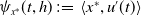 $\psi _{x^*}(t,h)\;:\!=\; \langle x^*, u'(t)\rangle$
on
$\psi _{x^*}(t,h)\;:\!=\; \langle x^*, u'(t)\rangle$
on
 $(t,u)\in A$
. As a limit of continuous functions
$(t,u)\in A$
. As a limit of continuous functions
 $\psi _{x^*}$
is a Borel function on
$\psi _{x^*}$
is a Borel function on
 $A$
and thus
$A$
and thus
 $\bar {\eta }$
measurable. Since
$\bar {\eta }$
measurable. Since
 $\mathcal{X}$
is separable, Pettis theorem ensures that
$\mathcal{X}$
is separable, Pettis theorem ensures that
 $\psi$
is a
$\psi$
is a
 $\bar {\eta }$
-measurable function. Now we can define the vector field
$\bar {\eta }$
-measurable function. Now we can define the vector field
 \begin{equation*}\boldsymbol{v}_t(x)\;:\!=\; \int _{C(0,T;\;\mathcal{X})} u'(t) \text{d}\bar {\eta }_{x,t} \quad \text{ for } \bar {\mu }\text{-a.e.}\, (t,x)\in (0,T)\times \mathcal{X}.\end{equation*}
For clarity, we now indicate the varibles over which the
 $ess\,sup$
is taken in brackets after the respective measure. Using this notation we estimate
$ess\,sup$
is taken in brackets after the respective measure. Using this notation we estimate
 \begin{align*} \bar {\mu }-\operatorname*{ess\,sup} \| \boldsymbol{v}\| &= \bar {\mu }(x,t)-\operatorname*{ess\,sup} \left \| \int _{C(0,T;\;\mathcal{X})} u'(t) d\bar {\eta }_{x,t} (u)\right \|\\ &\leq \bar {\mu }(x,t)-\operatorname*{ess\,sup} \int _{C(0,T;\;\mathcal{X})} \left \|u'(t)\right \| d\bar {\eta }_{x,t} (u)\\&\leq \bar {\mu }(x,t)-\operatorname*{ess\,sup}\, \big (\bar {\eta }_{x,t} (u)-\operatorname*{ess\,sup} \left \|u'(t)\right \|\big )\\ &\leq \bar {\eta }(u,t)-\operatorname*{ess\,sup} \left \|u'(t)\right \| \lt +\infty , \end{align*}
and thus
 $\boldsymbol{v}\in L^\infty (\bar {\mu };\mathcal{X})$
, where the last inequality follows from Lemma E.3. By Jensen’s inequality we have for every
$\boldsymbol{v}\in L^\infty (\bar {\mu };\mathcal{X})$
, where the last inequality follows from Lemma E.3. By Jensen’s inequality we have for every
 $[a,b]\subset [0,T]$
,
$[a,b]\subset [0,T]$
,
 \begin{align} \begin{aligned} \int _a^b \|\boldsymbol{v}_t\|_{L^\infty (\mu _t;\mathcal{X})}\,\text{d}t&=\int _a^b \mu _t({x})-\operatorname*{ess\,sup} \| \boldsymbol{v}_t(x)\| \,\text{d}t\\&=\int _a^b \mu _t({x})-\operatorname*{ess\,sup} \left \|\int _{C(0,T;\;\mathcal{X})} u'(t) d\bar {\eta }_{x,t}\right \| \,\text{d}t\\ &\leq \int _a^b \mu _t({x})-\operatorname*{ess\,sup} \int _{C(0,T;\;\mathcal{X})} \left \|u'(t)\right \| d\bar {\eta }_{x,t} \,\text{d}t\\ &\leq \int _a^b \mu _t({x})-\operatorname*{ess\,sup}\, \bar {\eta }_{x,t}(u)-\operatorname*{ess\,sup}\left \|u'(t)\right \| \,\text{d}t\\ &=\int _a^b \eta (u)-\operatorname*{ess\,sup} \| u'(t)\| \,\text{d}t=\int _a^b |\mu '|(t)\,\text{d}t. \end{aligned} \end{align}
such that
 $\|\boldsymbol{v}_t\|_{L^p(\mu _t;\mathcal{X})}\leq |\mu |'(t)$
for a.e.
$\|\boldsymbol{v}_t\|_{L^p(\mu _t;\mathcal{X})}\leq |\mu |'(t)$
for a.e.
 $t\in (0,T)$
. In the last inequality we used the fact, that
$t\in (0,T)$
. In the last inequality we used the fact, that
 $\,\text{d}\eta = d\bar {\eta }_{x,t} \,\text{d}\mu _t$
holds for a.e.
$\,\text{d}\eta = d\bar {\eta }_{x,t} \,\text{d}\mu _t$
holds for a.e.
 $t\in (0,T)$
together with Lemma E.3. For more rigorous justifications regarding measurably and integrability of all involved quantities, we refer to [Reference Lisini62, Theorem 7]. To show that
$t\in (0,T)$
together with Lemma E.3. For more rigorous justifications regarding measurably and integrability of all involved quantities, we refer to [Reference Lisini62, Theorem 7]. To show that
 $(\mu ,\boldsymbol{v})\in \mathrm{EC}^\infty (\mathcal{X})$
we take
$(\mu ,\boldsymbol{v})\in \mathrm{EC}^\infty (\mathcal{X})$
we take
 $\varphi \in C^1_b(\mathcal{X})$
and observe that
$\varphi \in C^1_b(\mathcal{X})$
and observe that
 $t\rightarrow \int _{\mathcal{X}} \varphi (x) \,\text{d}\mu _t(x)$
is absolutely continuous, since for
$t\rightarrow \int _{\mathcal{X}} \varphi (x) \,\text{d}\mu _t(x)$
is absolutely continuous, since for
 $\gamma \in \Gamma _0(\mu _t,\mu _s)$
 \begin{align*} \left |\int _{\mathcal{X}} \varphi \,\text{d}\mu _t -\int _{\mathcal{X}} \varphi \,\text{d}\mu _s\right |\leq \int _{\mathcal{X}\times \mathcal{X}} |\varphi (x)-\varphi (\tilde {x})|d\gamma \leq \\ \sup _{x\in \mathcal{X}} \|D\varphi (x)\| \int _{\mathcal{X}\times \mathcal{X}} \|x-\tilde {x}\|d\gamma \leq \sup _{x\in \mathcal{X}} \|D\varphi (x)\| W_\infty (\mu _t,\mu _s). \end{align*}
Further,
 \begin{align*} \int _{\mathcal{X}} \varphi \,\text{d}\mu _t&-\int _{\mathcal{X}} \varphi \,\text{d}\mu _s=\int _{C(0,T;\;\mathcal{X})} \varphi (u(t))-\varphi (u(s))\,\text{d}\eta (u)\\&= \int _{C(0,T;\;\mathcal{X})} \langle D\varphi (u(s)),u(t)-u(s)\rangle \,\text{d}\eta (u)+\int _{C(0,T;\;\mathcal{X})} \|u(t)-u(s)\| \omega _{u(s)}(u(t)) \,\text{d}\eta (u)\\&= \int _{C(0,T;\;\mathcal{X})} \langle D\varphi (u(s)),\int _s^t u'(r)\,\text{d}r\rangle \,\text{d}\eta (u)+\int _{C(0,T;\;\mathcal{X})} \|u(t)-u(s)\| \omega _{u(s)}(u(t)) \,\text{d}\eta (u) \end{align*}
where
 \begin{equation*} \omega _x(y)=\frac {\varphi (y)-\varphi (x)-\langle D\varphi (u(x)),y-x\rangle }{\|y-x\|}.\end{equation*}
We observe
 \begin{equation*}\frac {1}{t-s}\langle D\varphi (u(s)),\int _s^t u'(r)\,\text{d}r\rangle \rightarrow \langle D\varphi (u(s)), u'(s)\rangle \quad \text{for } \eta \text{-a.e. } u\end{equation*}
and
 \begin{equation*} \frac {\|u(t)-u(s)\|}{t-s} \omega _{u(s)}(u(t)) \rightarrow 0 \quad \text{for } \eta \text{-a.e. } u \end{equation*}
and have for
 $\eta$
-a.e.
$\eta$
-a.e.
 $u$
the upper bounds
$u$
the upper bounds
 \begin{align*} \frac {1}{|t-s|}|\langle D\varphi (u(s)),\int _s^t u'(r)\,\text{d}r\rangle | &\leq \sup _{x\in \mathcal{X}} \|D\varphi (x)\|_* \frac {\left \|\int _s^t u'(r)\,\text{d}r\right \|}{|s-t|}\\&\leq \sup _{x\in \mathcal{X}} \|D\varphi (x)\|_* \operatorname*{ess\,sup}_{r\in [0,T]} |\mu '|(r)\lt +\infty \end{align*}
and
 \begin{align*} \frac {\|u(t)-u(s)\|}{|t-s|} |\omega _{u(s)}(u(t))|&\leq \operatorname*{ess\,sup}_{r\in [0,T]}|\mu '|(r) \left (\frac {|\varphi (u(t))-\varphi (u(s))|}{\|u(t)-u(s)\|}+\frac {|\langle D \varphi (u(s)),u(t)-u(s)\rangle |}{\|u(t)-u(s)\|}\right )\\&\leq \operatorname*{ess\,sup}_{r\in [0,T]}|\mu '|(r)\, 2\mathrm {Lip}(\varphi )\lt +\infty . \end{align*}
Dividing by
 $t-s$
and passing to the limit
$t-s$
and passing to the limit
 $t\rightarrow s$
by using Lebesgue theorem, we obtain
$t\rightarrow s$
by using Lebesgue theorem, we obtain
 \begin{align*} \frac {\text{d}}{ds} \int _{\mathcal{X}} \varphi \,\text{d}\mu _s=\int _{C(0,T;\;\mathcal{X})} \langle D \varphi (u(s)),u'(s)\rangle \,\text{d}\eta (u)=\int \langle D \varphi , \boldsymbol{v} _t\rangle \,\text{d}\mu _t \quad \text{for a.e. } s\in (0,T). \end{align*}
This pointwise derivative corresponds to the distributional derivative and we obtain
 $(\mu ,\boldsymbol{v})\in \mathrm{EC}^\infty (\mathcal{X})$
.
$(\mu ,\boldsymbol{v})\in \mathrm{EC}^\infty (\mathcal{X})$
.
Similarly, we can adapt [Reference Lisini62, Theorem 8] to the case
 $p=\infty$
, which we again show by reusing most of the arguments from the corresponding proof in [Reference Lisini62].
$p=\infty$
, which we again show by reusing most of the arguments from the corresponding proof in [Reference Lisini62].
Proof of Theorem
4.11. This theorem was proven in [Reference Lisini62, Theorem 8] for
 $p\in (1,+\infty )$
and can easily be extended to the case
$p\in (1,+\infty )$
and can easily be extended to the case
 $p=+\infty$
. Let
$p=+\infty$
. Let
 $(\mu _t)_{t\in [0,T]}$
be a family of measures in
$(\mu _t)_{t\in [0,T]}$
be a family of measures in
 $\mathcal{P}_\infty (\mathcal{X})$
and for each
$\mathcal{P}_\infty (\mathcal{X})$
and for each
 $t$
we have a velocity field
$t$
we have a velocity field
 $\boldsymbol{v}_t\in L^\infty (\mu _t;\mathbb{R}^d)$
with
$\boldsymbol{v}_t\in L^\infty (\mu _t;\mathbb{R}^d)$
with
 $ ess\,sup \|\boldsymbol{v}_t\|_{L^\infty (\mu _t)} \lt \infty$
, solving the continuity equation in the sense of distributions. Since
$ ess\,sup \|\boldsymbol{v}_t\|_{L^\infty (\mu _t)} \lt \infty$
, solving the continuity equation in the sense of distributions. Since
 \begin{align*} \|\boldsymbol{v}\|_{L^p(\bar {\mu };\mathcal{X})} \leq T^{1/p} \operatorname*{ess\,sup} \|\boldsymbol{v} _t\|_{L^\infty (\mu _t)} \lt \infty \end{align*}
we can apply [Reference Lisini62, Theorem 8] (i.e., the statement of Theorem 4.11) for all
 $p\in (1,\infty )$
and get
$p\in (1,\infty )$
and get
 \begin{align*} |\mu '|_{(p)}(t)\leq \|\boldsymbol{v} _t\|_{L^p(\mu _t;\mathcal{X})} \text{ for a.e.} \ t\in (0,T) \text{ and all } p\in (1,\infty ). \end{align*}
Therefore,
 \begin{align*} W_p(\mu _t, \mu _s)\leq \int _t^s |\mu '|_{(p)}(\tilde {t}) d\tilde {t}\leq \int _t^s \|\boldsymbol{v} _t\|_{L^p(\mu _{\tilde {t}};\mathcal{X})} d\tilde {t}\leq \int _t^s \|\boldsymbol{v} _t\|_{L^\infty (\mu _{\tilde {t}};\mathcal{X})} d\tilde {t} \end{align*}
for all
 $t,s\in [0,T]$
with
$t,s\in [0,T]$
with
 $t\leq s$
and
$t\leq s$
and
 $p\in (1,\infty )$
, where
$p\in (1,\infty )$
, where
 $|\mu '|_{(p)}$
denotes the metric derivative of
$|\mu '|_{(p)}$
denotes the metric derivative of
 $\mu$
in
$\mu$
in
 $W_p$
. Taking the limit
$W_p$
. Taking the limit
 $p\to \infty$
, we get
$p\to \infty$
, we get
 \begin{align*} W_\infty (\mu _t, \mu _s)=\lim _{p\rightarrow \infty }W_p(\mu _t, \mu _s)\leq \int _t^s \| \boldsymbol{v} _t\|_{L^\infty (\mu _{\tilde {t}};\mathcal{X})} d\tilde {t} \end{align*}
for all
 $t,s\in [0,T]$
with
$t,s\in [0,T]$
with
 $t\leq s$
and thus by the minimality of the metric derivative, see Remark 1.2,
$t\leq s$
and thus by the minimality of the metric derivative, see Remark 1.2,
 \begin{align*} |\mu '|_{(\infty )}(t)\leq \| \boldsymbol{v} _t\|_{L^\infty (\mu _t;\mathcal{X})} \text{ for a.e. }t \in (0,T). \end{align*}
Lemma E.2.
Let
 $\mu$
be a Borel probability measure on
$\mu$
be a Borel probability measure on
 $\mathcal{X}$
and
$\mathcal{X}$
and
 $v: \mathcal{X} \rightarrow \mathcal{X}$
,
$v: \mathcal{X} \rightarrow \mathcal{X}$
,
 $\tilde {v}\;:\;\mathcal{X}\rightarrow \mathcal{X}$
be two
$\tilde {v}\;:\;\mathcal{X}\rightarrow \mathcal{X}$
be two
 $\mu$
-measurable functions with
$\mu$
-measurable functions with
 \begin{align*} \int \langle D\varphi (x),v(x)\rangle \,\text{d}\mu (x)=\int \langle D\varphi (x),\tilde {v}(x)\rangle \,\text{d}\mu (x) \quad \forall \varphi \in C^1_b(\mathcal{X}) \end{align*}
then
 \begin{align} \int \langle \xi , v(x)\rangle \,\text{d}\mu (x) =\int \langle \xi , \tilde {v}(x)\rangle \,\text{d}\mu (x) \quad \forall \xi \in \mathcal{X}^*. \end{align}
Proof. Let
 $g_n\;:\;\mathbb{R}\rightarrow \mathbb{R}$
be the function with
$g_n\;:\;\mathbb{R}\rightarrow \mathbb{R}$
be the function with
 $g(0)=0$
and
$g(0)=0$
and
 \begin{align*} g'(x)=\begin{cases} 0 & \text{for } |x|\gt n+1,\\ 1 & \text{for } |x|\lt n ,\\ n+1-x & \text{for } x\in [n,n+1],\\ n+1+x& \text{for } x \in [-(n+1),-n]. \end{cases} \end{align*}
Then for each
 $\xi \in \mathcal{X}^*$
we get
$\xi \in \mathcal{X}^*$
we get
 $G_n:x\mapsto g_n(\langle \xi , x\rangle )\in C^1_b(\mathcal{X})$
with
$G_n:x\mapsto g_n(\langle \xi , x\rangle )\in C^1_b(\mathcal{X})$
with
 $DG_n(x)=g_n'(\langle \xi ,x\rangle )\ \xi$
and
$DG_n(x)=g_n'(\langle \xi ,x\rangle )\ \xi$
and
 \begin{align*} \int g_n'(\langle \xi ,x\rangle )\langle \xi ,v(x)\rangle \,\text{d}\mu &=\int \langle D G_n(x),v(x)\rangle \,\text{d}\mu = \int \langle D G_n(x),\tilde {v}(x)\rangle \,\text{d}\mu \\&=\int g'_n(\langle \xi ,x\rangle )\langle \xi ,\tilde {v}(x)\rangle \,\text{d}\mu \end{align*}
Since for
 $n\rightarrow \infty$
we have
$n\rightarrow \infty$
we have
 $g'(\langle \xi ,x\rangle )\rightarrow 1$
pointwise we can apply the Lebesgue dominated convergence theorem (with the functions
$g'(\langle \xi ,x\rangle )\rightarrow 1$
pointwise we can apply the Lebesgue dominated convergence theorem (with the functions
 $|\langle \xi , v(x)\rangle |$
and
$|\langle \xi , v(x)\rangle |$
and
 $|\langle \xi , \tilde {v}(x)\rangle |$
as bound) to obtain (E.2).
$|\langle \xi , \tilde {v}(x)\rangle |$
as bound) to obtain (E.2).
The following lemma shows that the disintegration property can be transferred to an inequality for essential suprema. For more details on disintegration, we refer to [Reference Ambrosio, Gigli and Savaré2, Ch. 5.3] and [Reference Dellacherie and Meyer33, Ch. III-70]. The proof strategy is taken from [Reference Roith and Bungert85, Lemma 2] and amounts to controlling the null sets of the measures involved.
Lemma E.3.
Given
 $\mathcal{X}, \mathcal{Z}$
Radon separable metric spaces, a measure
$\mathcal{X}, \mathcal{Z}$
Radon separable metric spaces, a measure
 $\mu \in \mathcal{P}(\mathcal{X})$
, a Borel map
$\mu \in \mathcal{P}(\mathcal{X})$
, a Borel map
 $\pi \;:\;\mathcal{X}\to \mathcal{Z}$
and a disintegration
$\pi \;:\;\mathcal{X}\to \mathcal{Z}$
and a disintegration
 $\,\text{d}\mu = \,\text{d}\mu _z d\nu$
, with
$\,\text{d}\mu = \,\text{d}\mu _z d\nu$
, with
 $\nu =\pi _\#\mu$
and
$\nu =\pi _\#\mu$
and
 $\{\mu _z\}_{z\in \mathcal{Z}}\subset \mathcal{P}(\mathcal{X})$
being a family of probability measures, then we have that
$\{\mu _z\}_{z\in \mathcal{Z}}\subset \mathcal{P}(\mathcal{X})$
being a family of probability measures, then we have that
 \begin{align*} \mu ({x})-\operatorname*{ess\,sup} f(x) \geq \nu (z)-\operatorname*{ess\,sup}\, \mu _z({x})-\operatorname*{ess\,sup} f({x}) \end{align*}
for every Borel map
 $f\;:\;\mathcal{X}\to [0,\infty ]$
.
$f\;:\;\mathcal{X}\to [0,\infty ]$
.
Proof. Using the disintegration property for every Borel set
 $A$
, we obtain
$A$
, we obtain
 \begin{align*} \mu (A) = 0 \quad \Leftrightarrow \quad \mu _z(A) \text{ for } \nu -\text{a.e. } z\in \mathcal{Z}. \end{align*}
Now assume that
 $\mu (A) = 0$
, then we know that there exists a Borel set
$\mu (A) = 0$
, then we know that there exists a Borel set
 $B\subset \mathcal{Z}$
with
$B\subset \mathcal{Z}$
with
 $\nu (B)=0$
and
$\nu (B)=0$
and
 $\mu _z(A) =0$
for all
$\mu _z(A) =0$
for all
 $z\in \mathcal{Z}\setminus B$
. Therefore,
$z\in \mathcal{Z}\setminus B$
. Therefore,
 \begin{align*} \sup _{x\in \mathcal{X}\setminus A} f({x}) &\geq \inf _{\tilde {A}\;:\;\mu _z(\tilde {A})=0} \sup _{x\in \mathcal{X}\setminus \tilde {A}} f({x}) = \mu _z({x})-\operatorname*{ess\,sup} f({x}) \qquad \text{ for all } z\in \mathcal{Z}\setminus B\\ \Rightarrow \sup _{x\in \mathcal{X}\setminus A} f({x}) &\geq \sup _{z\in \mathcal{Z}\setminus B}\, \mu _z({x})-\operatorname*{ess\,sup} f({x})\\ &\geq \inf _{\tilde {B}\;:\;\nu (\tilde {B})=0}\sup _{z\in \mathcal{Z}\setminus \tilde {B}} \mu _z({x})-\operatorname*{ess\,sup} f({x})\\ &= \nu (z)-\operatorname*{ess\,sup}\, \mu _z({x})-\operatorname*{ess\,sup}\, f({x}) \end{align*}
and since this holds for every
 $\mu$
-null set
$\mu$
-null set
 $A$
, we can take the infimum to obtain
$A$
, we can take the infimum to obtain
 \begin{align*} \mu ({x})-\operatorname*{ess\,sup} f({x}) = \inf _{A:\mu (A)=0}\sup _{x\in \mathcal{X}\setminus A} f({x}) \geq \nu (z)-\operatorname*{ess\,sup}\, \mu _z({x})-\operatorname*{ess\,sup} f({x}). \end{align*}
Lemma E.4.
Let
 $\eta \in \mathcal{P}(C(0,T;\;\mathcal{X}))$
, then we have that
$\eta \in \mathcal{P}(C(0,T;\;\mathcal{X}))$
, then we have that
 \begin{align*} \eta (u)-\operatorname*{ess\,sup} \left |u'\right |(t) \leq 1\quad &\text{for a.e. }t\in (0,T)\Longleftrightarrow \operatorname*{ess\,sup}_{t\in (0,T)}\, \left |u'\right |(t)\leq 1\quad &\text{for } \eta \text{ a.e. } u \in C(0,T;\;\mathcal{X}). \end{align*}
Proof. Choosing
 $\psi =\chi _{[0,1]}$
, and observing that
$\psi =\chi _{[0,1]}$
, and observing that
 $\psi (|u'|(t))$
is
$\psi (|u'|(t))$
is
 $\bar {\eta }$
-measurable (see [Reference Lisini63, Eq. (55)]) implies
$\bar {\eta }$
-measurable (see [Reference Lisini63, Eq. (55)]) implies
 \begin{align*} \eta (u)-\operatorname*{ess\,sup} \left |u'\right |(t) \leq 1\quad &\text{for a.e. }t\in (0,T) \\&\Longleftrightarrow \int _{C(0,T,\mathcal{X})} \psi (\left |u'\right |(t)) \,\text{d}\eta (u) = 0\quad \text{for a.e. }t\in (0,T)\\ \Longleftrightarrow \int _0^T \int _{C(0,T,\mathcal{X})} \psi (\left |u'\right |(t)) \,\text{d}\eta (u)\,\text{d}t = 0 &\Longleftrightarrow \int _{C(0,T,\mathcal{X})} \int _0^T \psi (\left |u'\right |(t)) \,\text{d}\eta (u)\,\text{d}t = 0 \\ \Longleftrightarrow \int _{C(0,T,\mathcal{X})} \int _0^T \psi (\left |u'\right |(t))\,\text{d}t \,\text{d}\eta (u) = 0 &\Longleftrightarrow \int _0^T \psi (\left |u'\right |(t))\,\text{d}t = 0\quad \text{for }\eta \text{ a.e. } u \in C(0,T;\;\mathcal{X})\\ \Longleftrightarrow \operatorname*{ess\,sup}_{t\in (0,T)}\, \left |u'\right |(t)\leq 1\quad &\text{for } \eta \text{ a.e. } u \in C(0,T;\;\mathcal{X}), \end{align*}
where we use Fubini–Tonelli theorem to change the order of integration.
F Multivalued correspondences
For multivalued correspondences, generalizations of continuity and measurability can be defined. We use the definitions from [Reference Charalambos and Aliprantis24]. In the following, we write
 $\varphi \;:\;\mathcal{X} \rightrightarrows \mathcal{Z}$
to denote a mapping
$\varphi \;:\;\mathcal{X} \rightrightarrows \mathcal{Z}$
to denote a mapping
 $\varphi \;:\;\mathcal{X}\to 2^{\mathcal{Z}}$
.
$\varphi \;:\;\mathcal{X}\to 2^{\mathcal{Z}}$
.
Definition F.1 (Weak measurability). Let
 $(S,\Sigma )$
be a measurable space and
$(S,\Sigma )$
be a measurable space and
 $\mathcal{X}$
be a topological space. We say that a correspondence
$\mathcal{X}$
be a topological space. We say that a correspondence
 $\varphi : S \rightrightarrows \mathcal{X}$
is weakly measurable, if
$\varphi : S \rightrightarrows \mathcal{X}$
is weakly measurable, if
 \begin{equation*} \varphi ^l(G)\in \Sigma \text{ for all open sets } G \text{ of }\mathcal{X},\end{equation*}
where
 \begin{equation} \varphi ^l(G)\;:\!=\; \{s\in S| \varphi (s) \cap G\neq \emptyset \} \end{equation}
is the so-called lower inverse.
Definition F.2 (Measurability). Let
 $(S,\Sigma )$
be a measurable space and
$(S,\Sigma )$
be a measurable space and
 $\mathcal{X}$
a topological space. We say that a correspondence
$\mathcal{X}$
a topological space. We say that a correspondence
 $\varphi : S \rightrightarrows \mathcal{X}$
is measurable, if
$\varphi : S \rightrightarrows \mathcal{X}$
is measurable, if
 \begin{equation*} \varphi ^l(F)\in \Sigma \text{ for all closed sets } F \text{ of }\mathcal{X}.\end{equation*}
The next theorem is known as the measurable maximum theorem, where we refer to [Reference Charalambos and Aliprantis24, Theorem 18.19] for the proof of this statement.
Theorem F.3 (Measurable maximum theorem). Let
 $\mathcal{X}$
be a separable metrizable space and
$\mathcal{X}$
be a separable metrizable space and
 $(S,\Sigma )$
a measurable space. Let
$(S,\Sigma )$
a measurable space. Let
 $\varphi : S \rightrightarrows \mathcal{X}$
be a weakly measurable correspondence with nonempty compact values, and suppose
$\varphi : S \rightrightarrows \mathcal{X}$
be a weakly measurable correspondence with nonempty compact values, and suppose
 $f:S\times \mathcal{X}\rightarrow \mathbb{R}$
is a Carathéodory function. Define the value function
$f:S\times \mathcal{X}\rightarrow \mathbb{R}$
is a Carathéodory function. Define the value function
 $m:S\rightarrow \mathbb{R}$
by
$m:S\rightarrow \mathbb{R}$
by
 \begin{equation*}m(s)=\max _{x\in \varphi (s)}f(s,x),\end{equation*}
and the correspondence
 $\mu : S\rightrightarrows \mathcal{X}$
of maximizers by
$\mu : S\rightrightarrows \mathcal{X}$
of maximizers by
 \begin{equation*}\mu (s)=\{x\in \varphi (s): f(s,x)=m(s)\}.\end{equation*}
Then
-
• The value function
$m$
is measurable.
-
• The “argmax” correspondence
$\mu$
has nonempty and compact values.
-
• The “argmax” correspondence
$\mu$
is measurable and admits a measurable selector.


G Calculations for distributional adversaries
For completeness, we state all lemmas used in section 5.2 here. Those lemmas correspond to a lemma proven in section section 4.3 and are only adapted to the setting of the transport distance
 $D$
.
$D$
.
Lemma G.1.
Let
 $\mathcal{X}\times \mathcal{Y} = {\mathbb{R}}^d\times {\mathbb{R}}^m$
, then the correspondence
$\mathcal{X}\times \mathcal{Y} = {\mathbb{R}}^d\times {\mathbb{R}}^m$
, then the correspondence
 \begin{align*} \boldsymbol{r}_\varepsilon (x,y)=\operatorname*{arg\,min}_{(\tilde {{x}}, \tilde {y}):c(x,y,\tilde {{x}},\tilde {y})\leq \varepsilon } E(\tilde {x},\tilde {y})=\left (\operatorname*{arg\,min}_{\tilde {{x}}\in \overline {B_\varepsilon }({x})}E(\tilde {x},y),y\right ) \end{align*}
is measurable and admits a
 $\mathcal{B}(\mathcal{X}\times \mathcal{Y})$
-measurable selector. Further, for each measurable selector
$\mathcal{B}(\mathcal{X}\times \mathcal{Y})$
-measurable selector. Further, for each measurable selector
 $r_\varepsilon \;:\;\mathcal{X}\times \mathcal{Y}\to \mathcal{X}$
we have the following,
$r_\varepsilon \;:\;\mathcal{X}\times \mathcal{Y}\to \mathcal{X}$
we have the following,
 \begin{align} (r_\varepsilon )_\#(\mu )\in \operatorname*{arg\,min}_{D(\mu ,\tilde {\mu })\leq \varepsilon } \int E(x,y) \,\mathrm{d}\mu (x,y). \end{align}
Proof. We consider the correspondence
 $\varphi \;:\;\mathcal{X}\times \mathcal{Y} \rightrightarrows \mathcal{X} \times \mathcal{Y}$
given by
$\varphi \;:\;\mathcal{X}\times \mathcal{Y} \rightrightarrows \mathcal{X} \times \mathcal{Y}$
given by
 \begin{align*} (x,y)\mapsto \left (\overline {B_\varepsilon }(x), y\right ) \end{align*}
where on the input space we use the topology induced by
 $\|\cdot \|_{\mathcal{X}}+\|\cdot \|_{\mathcal{Y}}$
and the output space is interpreted as the standard Euclidean space. Then we have that for every open set
$\|\cdot \|_{\mathcal{X}}+\|\cdot \|_{\mathcal{Y}}$
and the output space is interpreted as the standard Euclidean space. Then we have that for every open set
 $G\in \mathcal{X}$
that
$G\in \mathcal{X}$
that
 \begin{align*} \varphi ^l(G)=\{ (x,y)\in \mathcal{X}\times \mathcal{Y} \,:\, \left (\overline {B_\varepsilon }(x),y\right )\cap G\neq \emptyset \} \subset \mathcal{B}(\mathcal{X}\times \mathcal{Y}), \end{align*}
is open, which implies weak measurability, according to Definition F.1. Furthermore, we define the map
 $f(({x},y), (\tilde {x},\tilde {y}))\;:\!=\; -{E}(\tilde {x}, \tilde {y})$
which is a Carathéodory function, since
$f(({x},y), (\tilde {x},\tilde {y}))\;:\!=\; -{E}(\tilde {x}, \tilde {y})$
which is a Carathéodory function, since
 $E$
is continuous, with
$E$
is continuous, with
 \begin{align*} \max _{(\tilde {x},\tilde {y}) \in \varphi (x,y)} f(({x},y),(\tilde {x},\tilde {y})) = \min _{(\tilde {x},\tilde {y}):c(x,y, \tilde {{x}},\tilde {y})\leq \epsilon } -{E}(\tilde {x},\tilde {y}) \end{align*}
Then Theorem F.3 ensures the existence of a measurable selector. To prove (G.1) we observe that if
 $D(\mu ,\tilde {\mu })\leq \varepsilon$
, then for an optimal transport plan
$D(\mu ,\tilde {\mu })\leq \varepsilon$
, then for an optimal transport plan
 $\gamma \in \Gamma _0(\mu ,\tilde {\mu })$
, we know that
$\gamma \in \Gamma _0(\mu ,\tilde {\mu })$
, we know that
 $y=\tilde {y}$
and
$y=\tilde {y}$
and
 $\|{x}-\tilde {{x}}\|\leq \varepsilon$
,
$\|{x}-\tilde {{x}}\|\leq \varepsilon$
,
 $\gamma$
-a.e. Thus, using the disintegration
$\gamma$
-a.e. Thus, using the disintegration
 $d\gamma (x,y, \tilde {{x}},\tilde {y}) = d\psi _{x,y}(\tilde {{x}},\tilde {y}) \,\text{d}\mu (x,y)$
, for every
$d\gamma (x,y, \tilde {{x}},\tilde {y}) = d\psi _{x,y}(\tilde {{x}},\tilde {y}) \,\text{d}\mu (x,y)$
, for every
 $\tilde {\mu }$
with
$\tilde {\mu }$
with
 $D(\tilde {\mu },\mu )\leq \varepsilon$
, we calculate
$D(\tilde {\mu },\mu )\leq \varepsilon$
, we calculate
 \begin{align*} \int E(\tilde {x},\tilde {y}) d\tilde {\mu }(\tilde {x},\tilde {y})=\int E(\tilde {x},\tilde {y}) d\gamma (x,y,\tilde {x},\tilde {y})=\int \int E(\tilde {x},\tilde {y}) d\psi _{x,y}(\tilde {x},\tilde {y}) \,\text{d}\mu (x,y)\\ =\int \int E(\tilde {x},y) d\psi _{x,y}(\tilde {x},\tilde {y}) \,\text{d}\mu (x,y)\geq \int \int E(r_\varepsilon (x,y)) d\psi _{x,y}(\tilde {x},\tilde {y}) \,\text{d}\mu (x,y)=\int E(r_\varepsilon (x,y)) \,\text{d}\mu (x,y), \end{align*}
and (G.1) follows.
Lemma G.2.
Let
 $\mathcal{X}\times \mathcal{Y} = {\mathbb{R}}^d\times {\mathbb{R}}^m$
,
$\mathcal{X}\times \mathcal{Y} = {\mathbb{R}}^d\times {\mathbb{R}}^m$
,
 $E: \mathcal{X}\times \mathcal{Y} \rightarrow {\mathbb{R}}$
be in
$E: \mathcal{X}\times \mathcal{Y} \rightarrow {\mathbb{R}}$
be in
 $C^1(\mathcal{X}\times \mathcal{Y} )$
and
$C^1(\mathcal{X}\times \mathcal{Y} )$
and
 $\mu \in \mathcal{P}_\infty (\mathcal{X}\times \mathcal{Y})$
, then the metric slope with respect to
$\mu \in \mathcal{P}_\infty (\mathcal{X}\times \mathcal{Y})$
, then the metric slope with respect to
 $D$
is given by
$D$
is given by
 \begin{align*} |\partial \mathcal{E} |(\mu ) = \int \| \nabla _x E(x,y) \|_{\mathcal{X}^*} \,\text{d}\mu . \end{align*}
and
 $|\partial \mathcal{E}|$
is a strong upper gardient.
$|\partial \mathcal{E}|$
is a strong upper gardient.
Proof. We follow the arguments of Lemma 4.17. By Lemma G.1 we obtain
 \begin{align*} |\partial \mathcal{E}|(\mu )=\limsup _{\tau \rightarrow 0} \frac {\mathcal{E}(\mu )-\mathcal{E}_\tau (\mu )}{\tau }=\limsup _{\tau \rightarrow 0} \int \frac {E(x,y)-E(r_\tau (x,y))}{\tau } \,\text{d}\mu \\ =\int \lim _{\tau \rightarrow 0} \frac {E(x,y)-E(r_\tau (x,y))}{\tau } \,\text{d}\mu =\int \|\nabla _x E(x,y)\|_{\mathcal{X}^*}\,\text{d}\mu , \end{align*}
where dominated convergence together with Lemma 3.5 and Item 3 was used to draw the limit into the integral.
To prove that
 $|\partial \mathcal{E}|$
is a strong upper gradient we observe that
$|\partial \mathcal{E}|$
is a strong upper gradient we observe that
 $\| \nabla _x E(x,y) \|_{\mathcal{X}^*}$
is continuous and in particular lower semicontinuous such that we can use [Reference Ambrosio, Gigli and Savaré2, Lemma 5.1.7] to prove that the map
$\| \nabla _x E(x,y) \|_{\mathcal{X}^*}$
is continuous and in particular lower semicontinuous such that we can use [Reference Ambrosio, Gigli and Savaré2, Lemma 5.1.7] to prove that the map
 $t\mapsto |\partial \mathcal{E}|(\mu _t)$
is lower semicontinuous and thus Borel for every absolutely continuous curve
$t\mapsto |\partial \mathcal{E}|(\mu _t)$
is lower semicontinuous and thus Borel for every absolutely continuous curve
 $\mu _t$
. Assume that
$\mu _t$
. Assume that
 $\int _s^t \int _{\mathcal{X}\times \mathcal{Y}} \| \nabla _x E(x,y) \|_{\mathcal{X}^*} \,\text{d}\mu _r({x},y) |\mu '|(r) \,\text{d}r= \int _s^t \left |\partial \mathcal{E}\right |(\mu _r) |\mu '|(r)\,\text{d}r\lt +\infty$
, otherwise (1.4) holds trivially. By Theorem 4.7 we can estimate
$\int _s^t \int _{\mathcal{X}\times \mathcal{Y}} \| \nabla _x E(x,y) \|_{\mathcal{X}^*} \,\text{d}\mu _r({x},y) |\mu '|(r) \,\text{d}r= \int _s^t \left |\partial \mathcal{E}\right |(\mu _r) |\mu '|(r)\,\text{d}r\lt +\infty$
, otherwise (1.4) holds trivially. By Theorem 4.7 we can estimate
 \begin{align*} |\mathcal{E}(\mu _t)-\mathcal{E}(\mu _s)|&=\left |\int _{\mathcal{X}\times \mathcal{Y}} {E}(x,y)\,\text{d}\mu _t(x,y)-\int _{\mathcal{X}\times \mathcal{Y}} {E}(x,y)\,\text{d}\mu _s(x,y)\right |\\ &=\left |\int _{C(0,T;\;\mathcal{X}\times \mathcal{Y})} {E}(u(t))\,\text{d}\eta (u)-\int _{C(0,T;\;\mathcal{X})} {E}(u(s))d \eta (u)\right |\\ &\leq \int _{C(0,T;\;\mathcal{X}\times \mathcal{Y})}\left | {E}(u(t))- {E}(u(s))\right |d \eta (u)\\ &\leq \int _{C(0,T;\;\mathcal{X}\times \mathcal{Y})} \int _s^t \| \nabla _x E(u(r)) \|_{\mathcal{X}^*} \, |u'|(r)\,\text{d}r d \eta (u)\\ &\leq \int _s^t\int _{\mathcal{X}\times \mathcal{Y}} \| \nabla _x E(x,y) \|_{\mathcal{X}^*} \,\text{d}\mu _r(x,y) |\mu '|(r)\,\text{d}r\lt +\infty . \end{align*}
Here we use that
 $\eta$
is concentrated on
$\eta$
is concentrated on
 $AC^\infty (0,T;\;\mathcal{X}\times \mathcal{Y})$
and by the definition of the the extended distance
$AC^\infty (0,T;\;\mathcal{X}\times \mathcal{Y})$
and by the definition of the the extended distance
 $c(x,\tilde {x},y,\tilde {y})$
on
$c(x,\tilde {x},y,\tilde {y})$
on
 $\mathcal{X}\times \mathcal{Y}$
a curve
$\mathcal{X}\times \mathcal{Y}$
a curve
 $u(t)\in AC^\infty (0,T;\;\mathcal{X}\times \mathcal{Y})$
only moves in
$u(t)\in AC^\infty (0,T;\;\mathcal{X}\times \mathcal{Y})$
only moves in
 $\mathcal{X}$
-direction and for those curves
$\mathcal{X}$
-direction and for those curves
 $\| \nabla _x E(u(r)) \|_{\mathcal{X}^*}$
acts like a strong upper gradient.
$\| \nabla _x E(u(r)) \|_{\mathcal{X}^*}$
acts like a strong upper gradient.
H Details on numerical examples
Here, we give some details on the experiment that produces Figure 1, the source code is provided at github.com/TimRoith/AdversarialFlows.
H.1 Training the neural network
We sample
 $K=1000$
labelled data points
$K=1000$
labelled data points
 $(({x}_1,y_1),\ldots , ({x}_K,y_K))$
, with
$(({x}_1,y_1),\ldots , ({x}_K,y_K))$
, with
 ${x}_k\in {\mathbb{R}}^2, y_k\in \{0,1\}$
, from the two moons data set using the sci-kit package [Reference Pedregosa78], see Figure H1a.
${x}_k\in {\mathbb{R}}^2, y_k\in \{0,1\}$
, from the two moons data set using the sci-kit package [Reference Pedregosa78], see Figure H1a.
Visualization of the dataset and trained classifiers used in the experiments.

Using PyTorch [Reference Paszke, Gross and Chintala76], we then train a neural network using the architecture displayed in Figure H2 as proposed in [Reference Howard52], to obtain a mapping
 $h_\theta \;:\;{\mathbb{R}}^2\to [0,1]$
, parametrized by
$h_\theta \;:\;{\mathbb{R}}^2\to [0,1]$
, parametrized by
 $\theta$
. Here “Linear
$\theta$
. Here “Linear
 $d^l\to d^{l+1}$
” in the
$d^l\to d^{l+1}$
” in the
 $l$
th layer, denotes an affine linear mapping [Reference Rosenblatt86] given by
$l$
th layer, denotes an affine linear mapping [Reference Rosenblatt86] given by
 \begin{align*} z\mapsto W z + b, \qquad \text{with learnable parameters} \quad W\in {\mathbb{R}}^{d^{l+1}\times d^{l}}, b \in {\mathbb{R}}^{d^{l+1}} \end{align*}
the activation functions “ReLU” [Reference Fukushima42], “GeLU” [Reference Hendrycks and Gimpel51] and “Sigmoid” are defined entry-wise for
 $i=1,\ldots , n$
, as
$i=1,\ldots , n$
, as
 \begin{align*} \text{ReLU}(z_i) \;:\!=\; \max \{0, z_i\},\qquad \text{GeLU}(z_i) \;:\!=\; z_i\cdot \Phi (z_i),\qquad \text{Sigmoid}(z_i) \;:\!=\; \frac {1}{1 + \exp ({-}z_i)}, \end{align*}
where
 $\Phi$
denotes the cumulative distribution function of the standard normal distribution. Here, we included both ReLU and GeLU (as a smooth approximation) to have an activation function, typically used in practice and a differentiable approximation fitting into the framework of section 3.3. During training, we process batches of inputs
$\Phi$
denotes the cumulative distribution function of the standard normal distribution. Here, we included both ReLU and GeLU (as a smooth approximation) to have an activation function, typically used in practice and a differentiable approximation fitting into the framework of section 3.3. During training, we process batches of inputs
 $\mathbf{z} = (z^1,\ldots , z^B)$
, with
$\mathbf{z} = (z^1,\ldots , z^B)$
, with
 $z_i\in {\mathbb{R}}^{d^l}$
, where “Batch Norm (
$z_i\in {\mathbb{R}}^{d^l}$
, where “Batch Norm (
 $B$
)”, as proposed in [Reference Ioffe and Szegedy54], uses the entry-wise mean
$B$
)”, as proposed in [Reference Ioffe and Szegedy54], uses the entry-wise mean
 $\mu (\mathbf{z})_i \;:\!=\; \frac {1}{B}\sum _{b=1}^B z_i^b$
and variance
$\mu (\mathbf{z})_i \;:\!=\; \frac {1}{B}\sum _{b=1}^B z_i^b$
and variance
 $\sigma (\mathbf{z})_i \;:\!=\; \frac {1}{B}\sum _{b=1}^B (z_i^b - \mu (\vec z))^2$
and is defined as
$\sigma (\mathbf{z})_i \;:\!=\; \frac {1}{B}\sum _{b=1}^B (z_i^b - \mu (\vec z))^2$
and is defined as
 \begin{align*} z_i^b \mapsto \frac {z_i^b - \mu (\mathbf{z})_i}{\sqrt {\sigma (\mathbf{z})_i^2 + \epsilon }} \cdot \gamma _i + \beta _k, \qquad \text{with learnable parameters}\quad \gamma , \beta \in {\mathbb{R}}^{d^l}, \end{align*}
where
 $\epsilon =10^{-5}$
is a small constant, added for numerical stability. During inference, the mean and variance are replaced by an estimate over the whole dataset, such that the output does not depend on the batch it is given. In total,
$\epsilon =10^{-5}$
is a small constant, added for numerical stability. During inference, the mean and variance are replaced by an estimate over the whole dataset, such that the output does not depend on the batch it is given. In total,
 $\theta$
denotes the collection of weights
$\theta$
denotes the collection of weights
 $W$
, biases
$W$
, biases
 $b$
and batch norm parameters
$b$
and batch norm parameters
 $\gamma , \beta$
of all layers. For training, we consider the loss function
$\gamma , \beta$
of all layers. For training, we consider the loss function
 \begin{align} \mathcal{L}(\theta )= \frac {1}{2K} \sum _{k=1}^K \left |h_\theta ({x}_k) - y_k\right |^2, \end{align}
where we employ the Adam optimizer [Reference Kingma and Ba56], with standard learning rates, to approximate a minimizer. In each step, we employ a batched version of the function in (H.1), i.e., instead of using all data points at once, in each so-called epoch, we randomly sample disjoint subsets of
 $\{1,\ldots , K\}$
, of size
$\{1,\ldots , K\}$
, of size
 $B=100$
and only sum over these points. We run this training process for a total of
$B=100$
and only sum over these points. We run this training process for a total of
 $100$
epochs, to obtain a set of parameters
$100$
epochs, to obtain a set of parameters
 $\theta ^*$
, with a train loss of approximately
$\theta ^*$
, with a train loss of approximately
 $\mathcal{L}(\theta ^*)\approx 0.002$
for ReLU and
$\mathcal{L}(\theta ^*)\approx 0.002$
for ReLU and
 $\mathcal{L}(\theta ^*)\approx 0.009$
for GeLU. The trained mappings
$\mathcal{L}(\theta ^*)\approx 0.009$
for GeLU. The trained mappings
 $h_\theta$
are visualized in Figure H1 and b.
$h_\theta$
are visualized in Figure H1 and b.
The network architecture used in the examples.

H.2 Computing IGFSM and the minimizing movement scheme
We now detail the iteration as displayed in Figure 1, first for ReLU. Here, we choose the initial value
 ${x}^0 = (0.1, 0.55)$
, as it is close to the decision boundary, with
${x}^0 = (0.1, 0.55)$
, as it is close to the decision boundary, with
 $h_{\theta ^*}({x}^0)\approx 0.97$
, an adversarial budget of
$h_{\theta ^*}({x}^0)\approx 0.97$
, an adversarial budget of
 $\varepsilon =0.2$
and the energy
$\varepsilon =0.2$
and the energy
 \begin{align*} E({x})\;:\!=\; \left |h_{\theta ^*}({x}) - 1\right |^2 + \chi _{B_\varepsilon ^\infty ({x}^0)}. \end{align*}
IFGSM is an explicit iteration and can therefore be implemented directly, where the gradient is computed with the automatic differentiation tools of PyTorch. For the minimizing movement scheme MinMove, we need to solve the problem
 \begin{align*} {x}_\tau ^{k+1}\in \operatorname*{arg\,min}_{{x}\in \overline {B_\tau ^\infty }({x}_\tau ^k)\cap \overline {B_\varepsilon ^\infty }({x}^0)} E({x}) , \end{align*}
in each step. In order to avoid local minima, we do not employ a gradient based method here, but rather a particle based method, which allows exploring the full rectangle
 $\overline {B_\tau ^\infty }({x}_\tau ^k)$
. We use consensus based optimization (CBO) as proposed in [Reference Pinnau, Totzeck, Tse and Martin79], using the CBXPy package [Reference Bailo, Barbaro and Gomes4]. Concerning the hyperparameters, we choose
$\overline {B_\tau ^\infty }({x}_\tau ^k)$
. We use consensus based optimization (CBO) as proposed in [Reference Pinnau, Totzeck, Tse and Martin79], using the CBXPy package [Reference Bailo, Barbaro and Gomes4]. Concerning the hyperparameters, we choose
 $N=30$
particles, a noise scaling of
$N=30$
particles, a noise scaling of
 $\sigma =2$
, with standard isotropic noise, a time discretization parameter
$\sigma =2$
, with standard isotropic noise, a time discretization parameter
 $\,\text{d}t=0.01$
,
$\,\text{d}t=0.01$
,
 $\alpha =10^8$
and perform
$\alpha =10^8$
and perform
 $30$
update steps in each inner iteration. In order to ensure the budget constraint and the local restriction given by the step size
$30$
update steps in each inner iteration. In order to ensure the budget constraint and the local restriction given by the step size
 $\tau$
, we project the ensemble of the CBO iteration to the set
$\tau$
, we project the ensemble of the CBO iteration to the set
 \begin{align*} \overline {B^\infty _\varepsilon }({x}^0)\cap \overline {B^\infty _\tau }({x}^k_\tau ) \end{align*}
using the
 $\ell ^\infty$
projection, i.e., a clipping operation. We refer to [Reference Bungert, Hoffmann, Kim and Roith19] for a more detailed numerical study considering projections in CBO schemes, which also suggests the validity of our method here. We repeat the experiment for GeLU with a different initial value
$\ell ^\infty$
projection, i.e., a clipping operation. We refer to [Reference Bungert, Hoffmann, Kim and Roith19] for a more detailed numerical study considering projections in CBO schemes, which also suggests the validity of our method here. We repeat the experiment for GeLU with a different initial value
 ${x}^0=(0.45,0.3), h_{\theta ^*}({x}^0)\approx 0.74$
and budget
${x}^0=(0.45,0.3), h_{\theta ^*}({x}^0)\approx 0.74$
and budget
 $\varepsilon =0.25$
, which is displayed in Figure H3.
$\varepsilon =0.25$
, which is displayed in Figure H3.
The same experiment as in Figure 1, but using a net employing the GeLU activation function.

H.3 Convergence of the standard and semi-implicit scheme
In this section, we consider the error between the standard and the semi-implicit minimizing movement, which serves as a very basic validation of the numerical schemes. Our theoretical framework shows that both iterations converge to a
 $\infty$
-curve of maximum slope, which however is not available numerically. Instead, for
$\infty$
-curve of maximum slope, which however is not available numerically. Instead, for
 $n\in \mathbb{N}$
and
$n\in \mathbb{N}$
and
 $k\leq n$
, we can consider
$k\leq n$
, we can consider
 \begin{align*} \left \|x_{\mathrm {si},\tau _n}^k - {x}^k_{\tau _n}\right \|_\infty \leq \left \|x_{\mathrm {si},\tau _n}^k - u(k\cdot \tau _n)\right \|_\infty + \left \|{x}^k_{\tau _n} - u(k\cdot \tau _n)\right \|_\infty , \end{align*}
where
 ${x}^k_{\tau _n}$
fulfils the standard minimizing movement scheme and
${x}^k_{\tau _n}$
fulfils the standard minimizing movement scheme and
 $x_{\mathrm {si},\tau _n}^k=x_{\mathrm {IFGS},\tau }^{k}$
is given by (IFGSM), i.e., fulfils the semi-implicit scheme. Although our theory does not provide concrete estimates or rates of the error between IFGSM and the minimizing movement scheme, we perform a small numerical experiment using the setup from above. For each choice of
$x_{\mathrm {si},\tau _n}^k=x_{\mathrm {IFGS},\tau }^{k}$
is given by (IFGSM), i.e., fulfils the semi-implicit scheme. Although our theory does not provide concrete estimates or rates of the error between IFGSM and the minimizing movement scheme, we perform a small numerical experiment using the setup from above. For each choice of
 $\tau$
we sample
$\tau$
we sample
 $S=50$
different initial values
$S=50$
different initial values
 ${x}^{0,s}$
and compute the iterates
${x}^{0,s}$
and compute the iterates
 $x_{\mathrm {IFGS}}^{k,s}$
and
$x_{\mathrm {IFGS}}^{k,s}$
and
 ${x}^{k,s}_{\tau }$
for
${x}^{k,s}_{\tau }$
for
 $k\in \{1,\ldots , \lfloor 1/\tau \rfloor \}$
and compute the averaged maximal distance
$k\in \{1,\ldots , \lfloor 1/\tau \rfloor \}$
and compute the averaged maximal distance
 \begin{align} e_\tau \;:\!=\;\frac {1}{S}\sum _{s=1}^S \max _{k}\left \|x_{\mathrm {IFGS}}^{k,s} - {x}^{k,s}_\tau \right \|_\infty . \end{align}
The errors are plotted in Figure H4a. In both cases, the errors converge to zero; however, we observe that the order of convergence is higher for the GeLU function. We note that our theoretical results only provide a convergence statement for the differentiable case, therefore these results are in line with the analysis. In particular Lemma 3.12 requires a Lipschitz differentiable gradient. However, we hypothesize that the slower convergence in the ReLU case, actually comes from the non-implicit error as visualized in Figure H4b. There we mimic a situation enforced by the ReLU activation function. For
 $\tau \gt 0.1$
, the minimizing movement scheme always “jumps” across the non-differentiable line
$\tau \gt 0.1$
, the minimizing movement scheme always “jumps” across the non-differentiable line
 $x_1=0.1$
, to the corner where the minimum on
$x_1=0.1$
, to the corner where the minimum on
 $\overline {B_\tau ^\infty }({x}^0)$
is attained, which leads the following iterates to follow the gradient into the direction
$\overline {B_\tau ^\infty }({x}^0)$
is attained, which leads the following iterates to follow the gradient into the direction
 $(1,1)$
. However, in this case the actual flow is given as
$(1,1)$
. However, in this case the actual flow is given as
 $u(t)\;:\!=\; (t,0)$
, which, in this case, is more accurately prescribed by (FGSM). In this regard, a more exhaustive study, both empirically and theoretically is required, which is left for future work.
$u(t)\;:\!=\; (t,0)$
, which, in this case, is more accurately prescribed by (FGSM). In this regard, a more exhaustive study, both empirically and theoretically is required, which is left for future work.
Difference between IFGSM and the minimizing movement scheme.

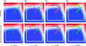


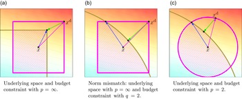


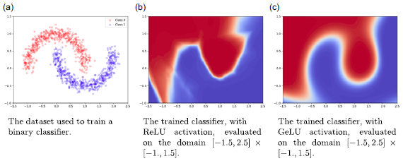
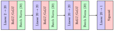
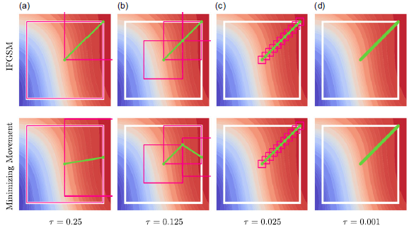
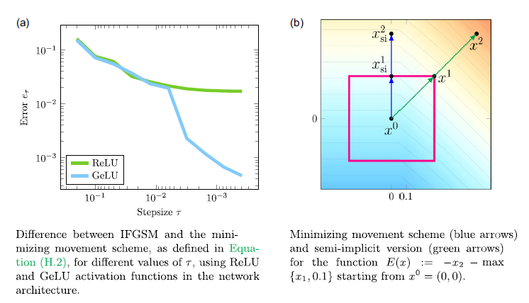

 Open access