


1. Introduction
Viscoplastic fluids are a class of non-Newtonian fluids characterised by the property that the material will not flow until the magnitude of the internal stress exceeds some threshold value (known as the ‘yield stress’). They behave as a solid for stresses below this. Deposits or extrusions of materials exhibiting viscoplastic behaviour are pervasive throughout industrial processes, geophysics and food science (Bird, Dai & Yarusso Reference Bird, Dai and Yarusso1983; Balmforth et al. Reference Balmforth, Burbidge, Craster, Salzig and Shen2000; Balmforth & Provenzale Reference Balmforth and Provenzale2001; Ancey Reference Ancey2007). Specific examples include the flow of concrete, mud, magma, ice, toothpaste and mayonnaise. Viscoplastic models are often a simplification of these materials’ rheology which may exhibit other complexities such as thixotropy, elasticity and non-isothermal behaviour, but are informative because the effects of a yield stress often dominate the macroscopic flow behaviour (Roussel et al. Reference Roussel, Lemaître, Flatt and Coussot2010).
This paper considers the slumping behaviour of a shallow, two-dimensional viscoplastic deposit atop a plate that oscillates horizontally. Such a situation may describe, for example, deposits of geological material under the action of seismic activity (Grelle, Revellino & Guadagno Reference Grelle, Revellino and Guadagno2011), compaction of concrete (Banfill, Teixeira & Craik Reference Banfill, Teixeira and Craik2011), piezoelectric energy harvesting (Maroofiazar & Farzam Reference Maroofiazar and Farzam2021) and the rheometry testing of complex materials and food stuffs (Cook & Brockhurst Reference Cook and Brockhurst1980; De Graef et al. Reference De Graef, Depypere, Minnaert and Dewettinck2011; Wang & Selomulya Reference Wang and Selomulya2022). Of particular note, recent experiments by Garg et al. (Reference Garg, Bergemann, Smith, Heil and Juel2021) investigate the slumping behaviour of deposits of Carbopol and molten chocolate, two complex yield-stress materials, atop a vertically vibrating plate. Chocolate exhibited prominent elasticity at early times, which subsided with its eventual mesoscopic re-organisation. Viscoplasticity was found to dominate the large time behaviour, as the deposit slumps towards an equilibrium shape. Carbopol was found to relax rapidly towards its equilibrium shape, while large-amplitude elastic oscillations persisted about this equilibrium. This nonlinear physical behaviour – much of which is unexplained by previous models – has ignited the drive for new research into forced oscillations of complex materials (Garg Reference Garg2022; Garg et al. Reference Garg, Akkinepally, Sarkar and Pattanayek2025).
This paper seeks to address two questions partially inspired by these experiments: Is qualitatively similar behaviour observed under horizontal oscillation? To what extent is the new equilibrium shape controlled by the yield stress alone? We deploy the simplest model for a viscoplastic fluid – the Bingham model (Bingham Reference Bingham1917) – and we apply no-slip boundary conditions at the oscillating plate. These choices enable us to tease out the impact of a yield stress on the flow physics. Our results can be extended to include Herschel–Bulkley fluids (Herschel & Bulkley Reference Herschel and Bulkley1926), which are defined by a power-law relationship between stress and strain above the yield stress. This paper aims to highlight aspects of the physical behaviour that are intrinsic only to the presence of a yield stress, however, and the additional detail of this power-law relationship is considered only peripherally to the main analysis. Similarly, the analysis of wall slip is beyond the scope of this paper, although we acknowledge its inclusion in our model may result in greater spread of the deposit (Jalaal, Balmforth & Stoeber Reference Jalaal, Balmforth and Stoeber2015).
Slow, thin viscoplastic flows over solid boundaries often take the form of a rigid plug migrating atop a basal shear flow of yielded material, and become fully arrested when the yield surface collides with the base everywhere (Huilgol & Georgiou Reference Huilgol and Georgiou2015). These flows are often analysed in the lubrication limit to quantify important physical processes such as the rate of front propagation and the form of the final arrested state. However, problems arise within the thin-film framework for viscoplastic flows, coined by Lipscomb & Denn (Reference Lipscomb and Denn1984) as the ‘lubrication paradox’. It is worth acknowledging that these yield surfaces are ‘fake’ because the seemingly rigid layers bounded by them are spatially varying ‘pseudo-plug’ flows that are not truly rigid. As demonstrated by Balmforth & Craster (Reference Balmforth and Craster1999), the deviation from truly rigid regions arises at higher asymptotic orders in $\varepsilon$
, the aspect ratio.
$\varepsilon$
, the aspect ratio.
Of particular relevance to the present work is the gravity-driven flow of a thin viscoplastic deposit on horizontal and inclined planes, which have arrested states derived by Liu & Mei (Reference Liu and Mei1989). On a stationary, horizontal plane, the final shape is given, in the lubrication limit, by
 \begin{align} h(x)= \sqrt {\frac {2 \tau _Y}{\rho g} (x_{\kern-1pt f}{(0)} - |{x}|)}, \end{align}
where $\tau _Y$
denotes the yield stress,
$\tau _Y$
denotes the yield stress, $\rho$
denotes the fluid density,
$\rho$
denotes the fluid density, $g$
is the value of gravitational acceleration and
$g$
is the value of gravitational acceleration and $\pm x_{\kern-1pt f}{(0)}$
are the contact points of the free surface with the plate (the notation
$\pm x_{\kern-1pt f}{(0)}$
are the contact points of the free surface with the plate (the notation $x_{\kern-1pt f}{(0)}$
is chosen to be consistent with a later definition), which are determined by asserting that the deposit must have area
$x_{\kern-1pt f}{(0)}$
is chosen to be consistent with a later definition), which are determined by asserting that the deposit must have area $A$
$A$
 \begin{align} {x_{\kern-1pt f}{(0)}}=\left (\frac {9 \rho g A^2}{32 \tau _Y}\right )^{1/3}. \end{align}
Cochard (Reference Cochard2007) observed the equilibrium shape (1.1) – and the slow approach to it – experimentally, and it was later confirmed by Hogg & Matson (Reference Hogg and Matson2009) that this final shape is only ever approached asymptotically. The error decays as $t^{-N}$
, (where
$t^{-N}$
, (where $N$
is the Herschel–Bulkley power-law index) at late times.
$N$
is the Herschel–Bulkley power-law index) at late times.
Arrested states in viscoplastic flows are typically not unique, as any free-surface profile which is kept below the yield stress everywhere will remain arrested (Balmforth et al. Reference Balmforth, Craster, Perona, Rust and Sassi2007; Hinton et al. Reference Hinton, Hewitt and Hogg2023b
). The thickness profile $h(x)$
in (1.1) is unique among the family of possible arrested states in the sense that it is on the ‘verge’ of yielding and so free-surface profiles ‘close’ to
$h(x)$
in (1.1) is unique among the family of possible arrested states in the sense that it is on the ‘verge’ of yielding and so free-surface profiles ‘close’ to $h(x)$
will approach it asymptotically.
$h(x)$
will approach it asymptotically.
The imposed horizontal oscillation considered in the present study additionally requires that inertia is included in the model. Fully time-dependent viscoplastic flows present a theoretical challenge, wherein the yield surfaces must be solved for in conjunction with the velocity and stress fields as a free-boundary problem. Analytical investigation into these flows has been limited, but important progress has been made for some unidirectional flow problems. Safronchik (Reference Safronchik1959) considered a channel flow of a Bingham fluid with a general initial velocity distribution and a time-dependent pressure gradient. A closed expression for the velocity field was found, although a nonlinear integral equation must be solved to obtain the position of the yield surface.
Progress has also been made on viscoplastic variations of some canonical time-dependent fluid mechanics problems: Stokes’ first problem (or the Rayleigh problem) and Stokes’ second problem (Stokes Reference Stokes1851). Fully analytical solutions were derived for the Rayleigh problem of an unbounded Herschel–Bulkley fluid in the cases that an impulsive velocity (Pascal Reference Pascal1989) or impulsive shear stress (Pascal Reference Pascal1992) is applied at the bottom interface. An analogue of the Rayleigh problem for a finite layer of viscoplastic fluid with a horizontal free surface was investigated by Hinton, Collis & Sader (Reference Hinton, Collis and Sader2022). A similar adaptation of Stokes’ second problem was investigated numerically and experimentally by Balmforth, Forterre & Pouliquen (Reference Balmforth, Forterre and Pouliquen2009), while an analytical exploration into the motion of its yield surfaces was conducted by Hinton et al. (Reference Hinton, Collis and Sader2023a ). Multiple yield surfaces may be present as the frequency of oscillation increases. Hewitt & Balmforth (Reference Hewitt and Balmforth2024) have analysed the oscillating layer problem for complex fluids. Piau & Piau (Reference Piau and Piau2007) have investigated the low oscillatory Reynolds limit of viscoplastic Couette and Poiseuille flows under the influence of longitudinally and transversely vibrating walls. The novelty of the set–up presented in this paper (compared with Stokes’ second problem) is the dynamically evolving free surface and finite, propagating fronts.
This paper is structured as follows. The theoretical background of the model of the oscillatory deposit is formulated in § 2. General numerical results are introduced in § 3. The low-frequency regime is investigated in § 4. The arrested shape is obtained in § 5. It is shown that this arrested state is identical to the down-slope arrested state derived by Liu & Mei (Reference Liu and Mei1989), and we derive the relationship between the inclination angle and the parameters of the plate oscillation. The asymptotic approach of the free surface to this arrested state is investigated in § 6. Concluding remarks are given in § 7. Various supplementary calculations are relegated to the appendices: a detailed exposition of the numerical scheme developed for this problem is presented in Appendix A. A scaling argument is presented to derive the temporal rate of asymptotic decay towards the arrested state of a Herschel–Bulkley fluid in Appendix B. A matched asymptotic expansion as the contact points are approached is outlined in Appendix C, and a numerical integration procedure is discussed in Appendix D.
2. Theoretical model
Schematic of the slumping of a viscoplastic material atop an oscillating plate. (a) Initial shape, which is then oscillated (in (b)), and slumps towards its arrested shape (c). The height of the deposit has been exaggerated for visibility.

We investigate the gravity-driven flow of a two-dimensional deposit of Bingham fluid of area $A$
lying atop a solid horizontal plate located at
$A$
lying atop a solid horizontal plate located at $z=0$
, with free-surface profile
$z=0$
, with free-surface profile $z=h(x,t)$
(see figure 1). The fluid is assumed to have completely slumped under gravity to its static profile (1.1) before the oscillatory plate motion commences. For
$z=h(x,t)$
(see figure 1). The fluid is assumed to have completely slumped under gravity to its static profile (1.1) before the oscillatory plate motion commences. For $t\geqslant 0$
the basal plate oscillates with velocity
$t\geqslant 0$
the basal plate oscillates with velocity $U_0 \sin (\omega t)$
in the
$U_0 \sin (\omega t)$
in the $x$
-direction, where
$x$
-direction, where $\omega$
is the oscillation frequency. The deposit then occupies the region between its two contact points
$\omega$
is the oscillation frequency. The deposit then occupies the region between its two contact points $x_{\kern-1pt f}^- (t) \leqslant x \leqslant x_{\kern-1pt f}^+ (t)$
. The fluid is incompressible and subject to Cauchy’s momentum equation and mass conservation, respectively,
$x_{\kern-1pt f}^- (t) \leqslant x \leqslant x_{\kern-1pt f}^+ (t)$
. The fluid is incompressible and subject to Cauchy’s momentum equation and mass conservation, respectively,
 \begin{align} \rho \left ( \frac {\partial \boldsymbol{u}}{\partial t} + \boldsymbol{u} \boldsymbol{\cdot }\boldsymbol{\nabla }\boldsymbol{u} \right ) &= -\boldsymbol{\nabla }p + \boldsymbol{\nabla }\boldsymbol{\cdot }\boldsymbol{\tau } - \rho g \hat {\boldsymbol{z}}, \\[-12pt] \nonumber \end{align}
 \begin{align} \boldsymbol{\nabla }\boldsymbol{\cdot }\boldsymbol{u} &= 0 , \\[10pt] \nonumber \end{align}
where $\boldsymbol{u}=(u, w)$
is the fluid velocity in the
$\boldsymbol{u}=(u, w)$
is the fluid velocity in the $x$
and
$x$
and $z$
directions,
$z$
directions, $\boldsymbol{\tau }=\tau _{\textit{ij}}$
is the deviatoric stress tensor and
$\boldsymbol{\tau }=\tau _{\textit{ij}}$
is the deviatoric stress tensor and $p$
is the pressure. The fluid obeys the Bingham constitutive law
$p$
is the pressure. The fluid obeys the Bingham constitutive law
where $\mu$
is the shear viscosity of the yielded material,
$\mu$
is the shear viscosity of the yielded material, $\dot {\gamma }_{\textit{ij}}$
is the strain-rate tensor, and
$\dot {\gamma }_{\textit{ij}}$
is the strain-rate tensor, and $|{\tau }|=\sqrt {\tau _{\textit{ij}} \tau _{\textit{ij}}/2}$
and
$|{\tau }|=\sqrt {\tau _{\textit{ij}} \tau _{\textit{ij}}/2}$
and $|{\dot {\gamma }}|=\sqrt { \dot {\gamma }_{\textit{ij}} \dot {\gamma }_{\textit{ij}}/2}$
are the second invariants of their respective tensors.
$|{\dot {\gamma }}|=\sqrt { \dot {\gamma }_{\textit{ij}} \dot {\gamma }_{\textit{ij}}/2}$
are the second invariants of their respective tensors.
The dynamical regime of interest is that of relatively thin deposits, so characteristic height and width scales are identified from the gravitationally slumped initial profile (1.1)–(1.2)
 \begin{align} H=A^{1/3} \left (\frac {\tau _Y}{\rho g}\right )^{1/3}, \qquad L=A^{2/3} \left (\frac {\tau _Y}{\rho g}\right )^{-1/3}. \end{align}
The aspect ratio $\varepsilon$
defines the ratio of these disparate length scales
$\varepsilon$
defines the ratio of these disparate length scales
 \begin{align} \varepsilon =\left (\frac {\tau _Y}{\rho g \sqrt {A}}\right )^{2/3}, \end{align}
and henceforth $\varepsilon \ll 1$
is assumed. This condition, specified by
$\varepsilon \ll 1$
is assumed. This condition, specified by $\rho g \sqrt {A} \gg \tau _Y$
, corresponds to a regime where the hydrostatic pressure gradients have sufficiently overcome the yield stress resulting in a relatively shallow free-surface profile under the action of gravity.
$\rho g \sqrt {A} \gg \tau _Y$
, corresponds to a regime where the hydrostatic pressure gradients have sufficiently overcome the yield stress resulting in a relatively shallow free-surface profile under the action of gravity.
The initial conditions are (Liu & Mei Reference Liu and Mei1989)
 \begin{align} \begin{split} u(x,z,0)=0, \quad h(x,0)= \sqrt {\frac {2 \tau _Y}{\rho g} (x_{\kern-1pt f}{(0)} - |{x}|)}, \\ \tau _{xz}(x,z,0)= \tau _Y \text{sgn}(x)\left [1-\frac {z}{\sqrt {\dfrac{2 \tau _Y}{\rho g} (x_{\kern-1pt f}{(0)} - |{x}|)}}\right ]\!. \end{split} \end{align}
The boundary conditions are
 \begin{align} \begin{split} u(x,0,t)=U_0 \sin (\omega t), \quad w(x,0,t)=0, \quad h(x_{\kern-1pt f}^{\pm } (t),t)=0, \\ w(x,h,t)= \frac {\partial h}{\partial t} + u(x,h,t) \frac {\partial h}{\partial x}, \qquad \tau _{xz}(x,h,t)=0. \end{split} \end{align}
It is assumed that the deposit is large enough to ignore capillary effects. This regime is specified by $\sigma \ll \rho \omega U_0 L^3/H$
, where
$\sigma \ll \rho \omega U_0 L^3/H$
, where $\sigma$
is the surface tension. Additionally, the height of the deposit is assumed to be much larger than the slip length, and so the no-slip condition is applied at the plate. We also assume that the elastic relaxation time of the material is much more rapid than the shear rate: the Weissenberg number
$\sigma$
is the surface tension. Additionally, the height of the deposit is assumed to be much larger than the slip length, and so the no-slip condition is applied at the plate. We also assume that the elastic relaxation time of the material is much more rapid than the shear rate: the Weissenberg number $\textit{Wi}=U_0\mu /\textit{GH} \ll 1$
, where
$\textit{Wi}=U_0\mu /\textit{GH} \ll 1$
, where $G$
is the elastic shear modulus of the material.
$G$
is the elastic shear modulus of the material.
A balance in the continuity (2.1b
) reveals that the horizontal and vertical velocity scales are $U_0$
and
$U_0$
and $ U_0 H/L$
, respectively. The system is non-dimensionalised by scaling the
$ U_0 H/L$
, respectively. The system is non-dimensionalised by scaling the $z$
-coordinate and free-surface profile with
$z$
-coordinate and free-surface profile with $H$
, the
$H$
, the $x$
-coordinate with
$x$
-coordinate with $L$
and time with the scale for oscillation
$L$
and time with the scale for oscillation $1/\omega$
. The pressure and stresses are non-dimensionalised according to their inertia-driven scales in (2.1a
), which are
$1/\omega$
. The pressure and stresses are non-dimensionalised according to their inertia-driven scales in (2.1a
), which are $\rho L \omega U_0$
and
$\rho L \omega U_0$
and $\rho H \omega U_0$
, respectively. Altogether,
$\rho H \omega U_0$
, respectively. Altogether,
 \begin{align} \begin{split} \hat {u}=\frac {u}{U_0}, \quad \hat {w}=\frac {L w}{U_0 H}, \quad \hat {t}=\omega t, \quad \hat {h}=\frac {h}{H}, \quad \hat {x}=\frac {x}{L}, \quad \hat {z}=\frac {z}{H}, \\ \hat {p}=\frac {p}{\rho L \omega U_0}, \quad {\left \{\hat {\tau }_{xx},\hat {\tau }_{xz},\hat {\tau }_{zz}\right \}=\frac {1}{\rho H \omega U_0} \left \{{\tau }_{xx},{\tau _{xz}},{\tau }_{zz}\right \}}, \end{split} \end{align}
where the hatted symbols signify the corresponding dimensionless variables.
Henceforth, the hats are omitted and all variables are taken to be non-dimensional. The associated dimensionless groups are
 \begin{align} \delta =\frac {U_0}{L\omega }, \qquad B=\frac {\tau _Y}{\rho H \omega U_0}, \qquad \alpha =\frac {\rho H^2 \omega }{\mu }. \end{align}
The dimensionless oscillation amplitude $\delta$
defines the ratio of the oscillation amplitude
$\delta$
defines the ratio of the oscillation amplitude $U_0 /\omega$
of the plate relative to the length of the initial deposit. The Bingham number
$U_0 /\omega$
of the plate relative to the length of the initial deposit. The Bingham number $B$
defines the ratio of the yield stress to the internal shear stress scale, and the oscillatory Reynolds number
$B$
defines the ratio of the yield stress to the internal shear stress scale, and the oscillatory Reynolds number $\alpha$
defines the time scale for momentum diffusion relative to the period of the oscillating plate. The quantity
$\alpha$
defines the time scale for momentum diffusion relative to the period of the oscillating plate. The quantity $\delta \alpha$
is the lubrication Reynolds number.
$\delta \alpha$
is the lubrication Reynolds number.
To simplify the analysis, the governing equations are expressed in coordinates co-moving with the plate
 \begin{align} \eta = x-\delta \left (1 - \cos t\right ),\qquad \mathscr{u}=u-\sin t. \end{align}
The deposit occupies the region $\eta _{\kern-1pt f}^{-} (t)\leqslant \eta \leqslant \eta _{\kern-1pt f}^{+} (t)$
, where
$\eta _{\kern-1pt f}^{-} (t)\leqslant \eta \leqslant \eta _{\kern-1pt f}^{+} (t)$
, where $\eta _{\kern-1pt f}^{\pm } (t)=x_{\kern-1pt f}^{\pm } (t)-\delta (1 - \cos t )$
denotes the contact points in the
$\eta _{\kern-1pt f}^{\pm } (t)=x_{\kern-1pt f}^{\pm } (t)-\delta (1 - \cos t )$
denotes the contact points in the $\eta$
frame. The dimensionless versions of the governing (2.1) in the moving frame are given by
$\eta$
frame. The dimensionless versions of the governing (2.1) in the moving frame are given by
 \begin{align} \frac {\partial \mathscr{u}}{\partial t} + \cos {t} + \delta \mathscr{u} \frac {\partial \mathscr{u}}{\partial \eta } + \delta w \frac {\partial \mathscr{u}}{\partial z}&=-\frac {\partial p}{\partial \eta } + \frac {\partial \tau _{\eta z}}{\partial z}+{\varepsilon } \frac {\partial \tau _{\eta \eta }}{\partial \eta }, \\[-12pt] \nonumber \end{align}
 \begin{align} \varepsilon ^2 \frac {\partial w}{\partial t} + \delta \varepsilon ^2 \mathscr{u} \frac {\partial w}{\partial \eta } + \delta \varepsilon ^2 w \frac {\partial w}{\partial z}&=-\frac {\partial p}{\partial z} + \varepsilon ^2 \frac {\partial \tau _{\eta z}}{\partial \eta }+{\varepsilon } \frac {\partial \tau _{z z}}{\partial z} - B, \\[-12pt] \nonumber \end{align}
 \begin{align} \frac {\partial \mathscr{u}}{\partial \eta } + \frac {\partial w}{\partial z} &= 0. \\[10pt] \nonumber \end{align}
The velocity $\mathscr{u}$
now vanishes at the plate, with the oscillatory motion manifesting as a forcing term,
$\mathscr{u}$
now vanishes at the plate, with the oscillatory motion manifesting as a forcing term, $\cos t$
, on the left-hand side of (2.10a
). In this paper, the model will be interrogated to leading order in
$\cos t$
, on the left-hand side of (2.10a
). In this paper, the model will be interrogated to leading order in $\varepsilon$
. In this limit, the vertical momentum (2.10b
) identifies that the pressure is hydrostatic. Additionally, the constitutive law (2.2) reveals that the normal stresses are
$\varepsilon$
. In this limit, the vertical momentum (2.10b
) identifies that the pressure is hydrostatic. Additionally, the constitutive law (2.2) reveals that the normal stresses are $\mathcal{O}{(\varepsilon )}$
smaller than the shear stress in yielded regions, so the yield criterion reduces to
$\mathcal{O}{(\varepsilon )}$
smaller than the shear stress in yielded regions, so the yield criterion reduces to $|{\tau }|=|{\tau _{\eta z}}| \gt \tau _Y$
. Finally, the only stress contribution in the leading-order shallow system is from the shear stress
$|{\tau }|=|{\tau _{\eta z}}| \gt \tau _Y$
. Finally, the only stress contribution in the leading-order shallow system is from the shear stress $\tau _{\eta z}$
, which will henceforth be written as
$\tau _{\eta z}$
, which will henceforth be written as $\tau$
. The horizontal momentum (2.10a
) now reduces to
$\tau$
. The horizontal momentum (2.10a
) now reduces to
 \begin{align} \frac {\partial \mathscr{u}}{\partial t} + \cos t +\delta \mathscr{u} \frac {\partial \mathscr{u}}{\partial \eta } + \delta w \frac {\partial \mathscr{u}}{\partial z}=-B \frac {\partial h}{\partial \eta } + \frac {\partial \tau }{\partial z}, \end{align}
with the constitutive law
Depth integrating the continuity (2.10c ) across the deposit and applying the kinematic condition in (2.6) at the free surface furnishes
 \begin{align} \frac {\partial h}{\partial t}+\delta \frac {\partial }{\partial \eta } \int _0^h \mathscr{u} \, \text{d}z =0. \end{align}
The dimensionless initial and boundary conditions are
 \begin{align} \mathscr{u}(\eta ,z,0) & =0, \ \ h(\eta ,0)= \sqrt {2 \left ( \eta _{\kern-1pt f}{(0)} - |{\eta }|\right )}, \nonumber \\ \tau (\eta ,z,0) & = B \, \text{sgn}(\eta )\left [1-\frac {z}{\sqrt {2 \left ( \eta _{\kern-1pt f}{(0)} - |{\eta }|\right )}}\right ] \!, \\[-28pt] \nonumber \end{align}
 \begin{align} \mathscr{u}(\eta ,0,t)= 0, \quad h(\eta _{\kern-1pt f}^{\pm } (t),t)=0, \quad \tau (\eta ,h,t)=0, \\[0pt] \nonumber \end{align}
where the scaled half-width of the initial free-surface profile is given by ${\eta _{\kern-1pt f}{(0)}}= (9/32 )^{1/3}$
. Since the shear stress vanishes at the free surface, there must exist a rigid layer adjacent to the free surface in which
${\eta _{\kern-1pt f}{(0)}}= (9/32 )^{1/3}$
. Since the shear stress vanishes at the free surface, there must exist a rigid layer adjacent to the free surface in which $|{\tau }| \leqslant B$
. An equation for the uppermost yield surface
$|{\tau }| \leqslant B$
. An equation for the uppermost yield surface $Y_1$
which bounds this rigid region from below may be derived by integrating the rigid momentum (2.11) over the region
$Y_1$
which bounds this rigid region from below may be derived by integrating the rigid momentum (2.11) over the region $Y_1 (\eta ,t) \lt z \lt h(\eta ,t)$
, giving (Sekimoto Reference Sekimoto1993)
$Y_1 (\eta ,t) \lt z \lt h(\eta ,t)$
, giving (Sekimoto Reference Sekimoto1993)
 \begin{align} \frac {\partial \mathscr{u}}{\partial t}+\delta \mathscr{u} \frac {\partial \mathscr{u}}{\partial \eta }=\frac {\partial \mathscr{u}_R}{\partial t} +\delta \mathscr{u}_R \frac {\partial \mathscr{u}_R}{\partial \eta }=-\cos {t} - B \frac {\partial h}{\partial \eta } - \frac {B \, \text{sgn}{\left (\tau \right )}}{h-Y_1} \quad \text{at} \quad z=Y_1 (\eta ,t), \end{align}
where the subscript $R$
henceforth refers to the rigid region; that is,
$R$
henceforth refers to the rigid region; that is, $\mathscr{u}_R (\eta ,t)=\mathscr{u}(\eta ,Y_1(\eta ,t),t)$
is the velocity of the pseudo-plugged flow, or equivalently, the velocity at the free surface. Equation (2.15) is valid throughout the uppermost rigid layer. A single yield surface emerges from the plate when the basal stress breaches the yield stress, initially propagating upwards and then eventually downwards through the deposit, colliding with the plate when the material rigidifies there. Multiple yield surfaces – and accompanying rigid regions – may coexist if
$\mathscr{u}_R (\eta ,t)=\mathscr{u}(\eta ,Y_1(\eta ,t),t)$
is the velocity of the pseudo-plugged flow, or equivalently, the velocity at the free surface. Equation (2.15) is valid throughout the uppermost rigid layer. A single yield surface emerges from the plate when the basal stress breaches the yield stress, initially propagating upwards and then eventually downwards through the deposit, colliding with the plate when the material rigidifies there. Multiple yield surfaces – and accompanying rigid regions – may coexist if $\alpha$
is large, and
$\alpha$
is large, and $B$
is sufficiently small (Hinton et al. Reference Hinton, Collis and Sader2023a
). In this regime, momentum diffusion is sufficiently slow relative to the plate oscillation, so an additional yield surface may emerge at the plate before the yield surfaces already present in the deposit have collided with the plate. The yield surfaces are denoted
$B$
is sufficiently small (Hinton et al. Reference Hinton, Collis and Sader2023a
). In this regime, momentum diffusion is sufficiently slow relative to the plate oscillation, so an additional yield surface may emerge at the plate before the yield surfaces already present in the deposit have collided with the plate. The yield surfaces are denoted $z=Y_i (\eta ,t)$
for
$z=Y_i (\eta ,t)$
for $i=1,2,\ldots , N$
, with
$i=1,2,\ldots , N$
, with $Y_1 (\eta ,t) \gt Y_2(\eta ,t) \gt \ldots \gt Y_N(\eta ,t)$
for a fixed
$Y_1 (\eta ,t) \gt Y_2(\eta ,t) \gt \ldots \gt Y_N(\eta ,t)$
for a fixed $\eta$
. From (2.12), it follows that the strain rate
$\eta$
. From (2.12), it follows that the strain rate $\dot {\gamma }=\partial \mathscr{u} / \partial z$
, must be continuous at each yield surface. The velocity must also be continuous everywhere, and requiring equality of
$\dot {\gamma }=\partial \mathscr{u} / \partial z$
, must be continuous at each yield surface. The velocity must also be continuous everywhere, and requiring equality of $\mathscr{u}$
on each yield surface provides a condition coupling motion in the rigid and yielded regions, hence closing the initial-boundary-value problem (2.11–2.14).
$\mathscr{u}$
on each yield surface provides a condition coupling motion in the rigid and yielded regions, hence closing the initial-boundary-value problem (2.11–2.14).
3. Numerical results
In this section, we describe the numerical method and validate it against some of our asymptotic results. Numerical results are presented for a region of the $(B, \alpha , \delta )$
parameter space in which
$(B, \alpha , \delta )$
parameter space in which $\delta$
is small.
$\delta$
is small.
3.1. Numerical method
Equations (2.11–2.13) are solved numerically with respect to the initial and boundary conditions (2.14) for the free-surface profile $h(x,t)$
, shear stress
$h(x,t)$
, shear stress $\tau (x,z,t)$
and strain rate
$\tau (x,z,t)$
and strain rate $\dot {\gamma }=\partial \mathscr{u} / \partial z$
. The strategy relies on evolving
$\dot {\gamma }=\partial \mathscr{u} / \partial z$
. The strategy relies on evolving $\dot {\gamma }$
in time, and calculating
$\dot {\gamma }$
in time, and calculating $\tau$
using the inverse of the constitutive law (2.12)
$\tau$
using the inverse of the constitutive law (2.12)
 \begin{align} \dot {\gamma }=\alpha \, \text{sgn}{(\tau )} \left (|{\tau }|-B\right )\varTheta {(|{\tau }|-B)}, \end{align}
where $\varTheta (\boldsymbol{\cdot })$
is the Heaviside step function. The numerical method solves the stress on a grid that is fully two-dimensional. The momentum (2.11) is differentiated with respect to
$\varTheta (\boldsymbol{\cdot })$
is the Heaviside step function. The numerical method solves the stress on a grid that is fully two-dimensional. The momentum (2.11) is differentiated with respect to $z$
to obtain
$z$
to obtain
 \begin{align} \frac {\partial \dot {\gamma }}{\partial t}+\delta \mathscr{u}\frac {\partial \dot {\gamma }}{\partial \eta } + \delta w \frac {\partial \dot {\gamma }}{\partial z}=\frac {\partial ^2 \tau }{\partial z^2}, \end{align}
where the velocities are written in terms of the strain rate via
 \begin{align} \mathscr{u}=\int _0^z \dot {\gamma }(\eta ,z',t) \, \text{d} z', \qquad w=-\int _0^z \frac {\partial }{\partial \eta } \mathscr{u}(\eta ,z',t) \, \text{d} z'. \end{align}
By integrating the flux term in the conservation of mass (2.13) by parts, we obtain an equation for the evolution of the free surface in terms of $\dot {\gamma }$
, rather than
$\dot {\gamma }$
, rather than $\mathscr{u}$
 \begin{align} \frac {\partial h}{\partial t}=-\delta \frac {\partial }{\partial \eta } \int _0^h (h-z) \dot {\gamma } \, \text{d}z. \end{align}
This formulation avoids the need to explicitly determine the yield surfaces (see also Balmforth et al. Reference Balmforth, Forterre and Pouliquen2009). The basal velocity boundary condition (2.14b ) can be expressed in terms of the shear stress by substituting the condition into the momentum (2.11), so all of the relevant boundary conditions are
 \begin{align} \frac {\partial \tau }{\partial z} \bigg {\rvert }_{z=0}=\cos t + \frac {\partial h}{\partial \eta }, \qquad \tau \rvert _{z=h}=0 . \end{align}
with the initial conditions given in (2.14a ). Full details of the numerical implementation can be found in Appendix A.
3.2. Physical features
The free-surface profile at $t=1, 10, 100, 1000, 10\,000$
for twelve pairs of
$t=1, 10, 100, 1000, 10\,000$
for twelve pairs of $(B,\alpha )$
, and
$(B,\alpha )$
, and $\delta =0.05$
. The black lines represent the numerical solution for
$\delta =0.05$
. The black lines represent the numerical solution for $h$
, and the red dotted lines are the numerical integration of the low-
$h$
, and the red dotted lines are the numerical integration of the low- $\alpha$
asymptotic (4.5). The initial free-surface profile
$\alpha$
asymptotic (4.5). The initial free-surface profile $h{(\eta ,0)}$
is the blue dashed line and the arrested state
$h{(\eta ,0)}$
is the blue dashed line and the arrested state $h_{\infty }{(\eta )}$
(whose solution is derived in § 5) is the solid blue line. As
$h_{\infty }{(\eta )}$
(whose solution is derived in § 5) is the solid blue line. As $\alpha$
increases beyond
$\alpha$
increases beyond $\mathcal{O}(1)$
, the low-
$\mathcal{O}(1)$
, the low- $\alpha$
free-surface profile deviates from the numerical solution at early times. At later times, even for
$\alpha$
free-surface profile deviates from the numerical solution at early times. At later times, even for $\alpha \gt \mathcal{O}{(1)}$
, the free surface is well described by the low-
$\alpha \gt \mathcal{O}{(1)}$
, the free surface is well described by the low- $\alpha$
solution because the inertia is less significant.
$\alpha$
solution because the inertia is less significant.

Results for the evolution of the free-surface profile are presented in figure 2, captured at $t=1$
,
$t=1$
, $10$
,
$10$
, $100$
,
$100$
, $1000$
and
$1000$
and $10\,000$
for
$10\,000$
for $(\alpha ,B)\in \{0.05,0.5,5,20\}\times \{0.3,0.8,1.5\}$
. The deposit slumps away from its initial shape (the dashed blue line) towards a symmetric arrested state (the solid blue line). Larger
$(\alpha ,B)\in \{0.05,0.5,5,20\}\times \{0.3,0.8,1.5\}$
. The deposit slumps away from its initial shape (the dashed blue line) towards a symmetric arrested state (the solid blue line). Larger $\alpha$
values result in more rapid slumping, because momentum diffusion is suppressed and
$\alpha$
values result in more rapid slumping, because momentum diffusion is suppressed and $\mathscr{u}=\mathcal{O}{(1)}$
.
$\mathscr{u}=\mathcal{O}{(1)}$
.
Initially, the deformation of the free surface is confined to the centre of the deposit, driven by the discontinuity of the free-surface gradient at $\eta =0$
. Disturbances propagate laterally towards the contact points, reaching them when
$\eta =0$
. Disturbances propagate laterally towards the contact points, reaching them when $t \sim 1/\delta \alpha$
. In the early-time regime, where
$t \sim 1/\delta \alpha$
. In the early-time regime, where $t \leqslant \mathcal{O}{(1/\delta \alpha )}$
, the contact points are only weakly advanced by these disturbances while the free surface reshapes behind them, approximately presenting as a ‘waiting time solution’ (Gratton, Minotti & Mahajan Reference Gratton, Minotti and Mahajan1999). This phenomenon can be described more specifically by analysing the deposit at each front, where the free-surface gradients dominate (2.11) and (2.15) and the leading-order contact point evolution is described by
$t \leqslant \mathcal{O}{(1/\delta \alpha )}$
, the contact points are only weakly advanced by these disturbances while the free surface reshapes behind them, approximately presenting as a ‘waiting time solution’ (Gratton, Minotti & Mahajan Reference Gratton, Minotti and Mahajan1999). This phenomenon can be described more specifically by analysing the deposit at each front, where the free-surface gradients dominate (2.11) and (2.15) and the leading-order contact point evolution is described by
 \begin{align} \frac {\text{d} \eta _{\kern-1pt f}^{\pm }}{\text{d} t} \sim \lim _{\eta \rightarrow \eta _{f}^{\pm }} \frac {B \alpha \delta }{h} \frac {\partial h}{\partial \eta } \left (\frac {h Y_{1}^2}{2} - \frac {Y_{1}^3}{6}\right ), \qquad Y_1 \sim \text{max}\left \{0, \, h-\frac {1}{|{{\partial h}/{\partial \eta }}|} \right \}. \end{align}
Thus, the free surface about the contact points must take the form $h \propto (\eta ^{\pm }_f(t)-|{\eta }|)^{1/3}$
to propagate at the same asymptotic order as the free surface evolution, which is a common result for creeping gravity currents; see Perazzo & Gratton (Reference Perazzo and Gratton2003), Matson & Hogg (Reference Matson and Hogg2007) and Appendix C. Evidently the front propagation is sub-leading order at early times, until the disturbances reach the contact points and the fronts steepen accordingly.
$h \propto (\eta ^{\pm }_f(t)-|{\eta }|)^{1/3}$
to propagate at the same asymptotic order as the free surface evolution, which is a common result for creeping gravity currents; see Perazzo & Gratton (Reference Perazzo and Gratton2003), Matson & Hogg (Reference Matson and Hogg2007) and Appendix C. Evidently the front propagation is sub-leading order at early times, until the disturbances reach the contact points and the fronts steepen accordingly.
Prominent asymmetry is visible in the bulk of the free-surface profile during the first few oscillations when $\alpha$
is large. In addition, once the early-time regime is breached, additional asymmetry in the contact points is evident, driven by the ordering of each oscillation direction. This asymmetry becomes more pronounced with larger
$\alpha$
is large. In addition, once the early-time regime is breached, additional asymmetry in the contact points is evident, driven by the ordering of each oscillation direction. This asymmetry becomes more pronounced with larger $\delta \alpha$
, as evident from the propagation rate (3.6). As an aside, we observe that if
$\delta \alpha$
, as evident from the propagation rate (3.6). As an aside, we observe that if $\delta \alpha \gg 1$
, the initial ‘waiting time’ period is negligible and the contact points may advance during the first oscillation. A host of interesting nonlinear behaviour can occur in this regime. In particular, if
$\delta \alpha \gg 1$
, the initial ‘waiting time’ period is negligible and the contact points may advance during the first oscillation. A host of interesting nonlinear behaviour can occur in this regime. In particular, if $B$
is sufficiently large, the negative
$B$
is sufficiently large, the negative $\eta$
contact point may advance beyond the predicted arrested position, and the deposit appears to slump towards a separate, asymmetric arrested state. Analysis of this regime is beyond the scope of this paper, which we restrict to the case where
$\eta$
contact point may advance beyond the predicted arrested position, and the deposit appears to slump towards a separate, asymmetric arrested state. Analysis of this regime is beyond the scope of this paper, which we restrict to the case where $\delta \alpha$
is small.
$\delta \alpha$
is small.
In this case, a late-time regime is eventually reached wherein the free surface is close to its symmetric arrested state. Inertial forcing is almost entirely opposed by the yield stress, and little variation in the free surface occurs during a period of oscillation. Despite any pronounced early-time asymmetries, the deposit is only weakly asymmetric in this regime. Because inertial effects are relatively small, the behaviour is described by the dynamics in the low $\alpha$
case.
$\alpha$
case.
Numerical solutions of the free-surface profile at $t=1, 10, 100, 1000$
for
$t=1, 10, 100, 1000$
for $B=0.8$
,
$B=0.8$
, $\alpha =5$
and
$\alpha =5$
and $\delta =0.05$
, beginning from two different initial shapes with area of unity. The red curves indicate the behaviour with initial condition given in (2.14). The solutions for some elliptical initial conditions are given by the black curves: in (a) the ellipse is chosen to have the same initial width as in (2.14), while in (b) the ellipse is chosen to have the same maximum height as in (2.14). The dotted lines are the respective initial profiles.
$\delta =0.05$
, beginning from two different initial shapes with area of unity. The red curves indicate the behaviour with initial condition given in (2.14). The solutions for some elliptical initial conditions are given by the black curves: in (a) the ellipse is chosen to have the same initial width as in (2.14), while in (b) the ellipse is chosen to have the same maximum height as in (2.14). The dotted lines are the respective initial profiles.

The yield surfaces plotted beneath the free-surface profile when $t=5 \pi /4$
for sixteen pairs of
$t=5 \pi /4$
for sixteen pairs of $(B,\alpha )$
, and
$(B,\alpha )$
, and $\delta =0.05$
. The solid black lines are the free surfaces, and the black dot-dash lines are the yield surfaces, obtained from the numerical solution. The red dotted lines are low-
$\delta =0.05$
. The solid black lines are the free surfaces, and the black dot-dash lines are the yield surfaces, obtained from the numerical solution. The red dotted lines are low- $\alpha$
results for the free surfaces and yield surfaces, obtained from numerical integration of (4.3)–(4.5). The material immediately beneath the free surface is always rigid. The vertical grey dashed lines are at
$\alpha$
results for the free surfaces and yield surfaces, obtained from numerical integration of (4.3)–(4.5). The material immediately beneath the free surface is always rigid. The vertical grey dashed lines are at $\eta =\eta _{\kern-1pt f}{(0)}/2$
, where the spatial snapshot is taken, shown in figure 5.
$\eta =\eta _{\kern-1pt f}{(0)}/2$
, where the spatial snapshot is taken, shown in figure 5.

The yield surfaces plotted beneath the free-surface profile for $\pi \leqslant t \leqslant 3\pi$
at
$\pi \leqslant t \leqslant 3\pi$
at $\eta =\eta _{\kern-1pt f}{(0)}/2$
for sixteen pairs of
$\eta =\eta _{\kern-1pt f}{(0)}/2$
for sixteen pairs of $(B,\alpha )$
, and
$(B,\alpha )$
, and $\delta =0.05$
. The solid black lines are the free surfaces, and the black dot-dash lines are the yield surfaces, obtained from the numerical solution. The red dotted lines are low-
$\delta =0.05$
. The solid black lines are the free surfaces, and the black dot-dash lines are the yield surfaces, obtained from the numerical solution. The red dotted lines are low- $\alpha$
results for the free surfaces and yield surfaces, obtained from numerical integration of (4.3–4.5). The material immediately beneath the free surface is always rigid material, and the yield surfaces partition this region from the yielded material. The vertical grey dashed lines are at
$\alpha$
results for the free surfaces and yield surfaces, obtained from numerical integration of (4.3–4.5). The material immediately beneath the free surface is always rigid material, and the yield surfaces partition this region from the yielded material. The vertical grey dashed lines are at $t=5\pi /4$
, where the temporal snapshot is taken, shown in figure 4.
$t=5\pi /4$
, where the temporal snapshot is taken, shown in figure 4.

The sensitivity of the slumping dynamics to variations in the initial condition is explored in figure 3. We observe that, for initial profiles ‘above’ the arrested state, early-time discrepancies are eventually forgotten as the slumping trajectories relax to the same late-time shape. The heights of the yield surfaces and free surface at $t=5\pi /4$
are plotted in figure 4. Early-time contact point asymmetry is visible in the
$t=5\pi /4$
are plotted in figure 4. Early-time contact point asymmetry is visible in the $\alpha =20$
row, because
$\alpha =20$
row, because $\delta \alpha =1$
and so the early-time regime had subsided. The height of the yield surfaces and the free surface at
$\delta \alpha =1$
and so the early-time regime had subsided. The height of the yield surfaces and the free surface at $\eta = \eta _{\kern-1pt f}{(0)}/2$
during an early period of oscillation are presented in figure 5. The regimes observed in figure 5 are qualitatively similar to those described by Hinton et al. (Reference Hinton, Collis and Sader2023a
) for a horizontal free surface, although the addition of free-surface gradients introduces a spatial dependence that may suppress or support the growth of a yield surface in some region.
$\eta = \eta _{\kern-1pt f}{(0)}/2$
during an early period of oscillation are presented in figure 5. The regimes observed in figure 5 are qualitatively similar to those described by Hinton et al. (Reference Hinton, Collis and Sader2023a
) for a horizontal free surface, although the addition of free-surface gradients introduces a spatial dependence that may suppress or support the growth of a yield surface in some region.
For large $B$
,
$B$
, $h$
remains close to
$h$
remains close to $h(\eta ,0)$
and the yield surface is confined to a thin region above the plate. For
$h(\eta ,0)$
and the yield surface is confined to a thin region above the plate. For $B \gg 1$
, the deposit only yields in
$B \gg 1$
, the deposit only yields in $\eta \leqslant 0$
when
$\eta \leqslant 0$
when $\cos {t}\geqslant 0$
, and only yields in
$\cos {t}\geqslant 0$
, and only yields in $\eta \geqslant 0$
when
$\eta \geqslant 0$
when $\cos {t} \leqslant 0$
, because the oscillatory forcing is no longer large enough to overcome the yield stress when their signs are opposing (see figure 4 for
$\cos {t} \leqslant 0$
, because the oscillatory forcing is no longer large enough to overcome the yield stress when their signs are opposing (see figure 4 for $\alpha =0.05, 0.5$
and
$\alpha =0.05, 0.5$
and $B=0.8, 1.5$
).
$B=0.8, 1.5$
).
When $\alpha \gg 1$
and
$\alpha \gg 1$
and $B \geqslant \mathcal{O}(1)$
, momentum diffusion is slow relative to the plate oscillation, so the shear stress decays rapidly away from the plate. In this regime, the flow within the deposit is envisioned as a large plugged bulk moving atop a thin lubricating layer at the base (see figure 5 for
$B \geqslant \mathcal{O}(1)$
, momentum diffusion is slow relative to the plate oscillation, so the shear stress decays rapidly away from the plate. In this regime, the flow within the deposit is envisioned as a large plugged bulk moving atop a thin lubricating layer at the base (see figure 5 for $\alpha =5, 20$
and
$\alpha =5, 20$
and $B=0.8, 1.5$
). The large rigid layer permits instantaneous momentum transfer to the free surface, allowing the velocity of the plug to adopt the
$B=0.8, 1.5$
). The large rigid layer permits instantaneous momentum transfer to the free surface, allowing the velocity of the plug to adopt the $\mathcal{O}(1)$
values of the basal velocity and thus evolve the free surface more rapidly than the other regimes.
$\mathcal{O}(1)$
values of the basal velocity and thus evolve the free surface more rapidly than the other regimes.
Generally, smaller values of $B$
result in a larger proportion of the material becoming yielded at early times. When
$B$
result in a larger proportion of the material becoming yielded at early times. When $\alpha \gg 1$
and
$\alpha \gg 1$
and $B \lt \mathcal{O}(1)$
the velocity dissipates rapidly within the yielded region adjacent to the plate, dampening momentum transfer to the free surface. The thin rigid regions emanating from the plate take longer to reach the free surface, so multiple yield surfaces may exist in the bulk of the deposit if
$B \lt \mathcal{O}(1)$
the velocity dissipates rapidly within the yielded region adjacent to the plate, dampening momentum transfer to the free surface. The thin rigid regions emanating from the plate take longer to reach the free surface, so multiple yield surfaces may exist in the bulk of the deposit if $B$
is sufficiently small (for example, see figure 5 for
$B$
is sufficiently small (for example, see figure 5 for $\alpha =5, B=0.05$
; for
$\alpha =5, B=0.05$
; for $\alpha =20$
, multiple yield surfaces can be observed for
$\alpha =20$
, multiple yield surfaces can be observed for $B=0.05$
and
$B=0.05$
and $B=0.3$
). This only occurs where the hydrostatic pressure gradients are negligible, however; in a region about the contact points the hydrostatic pressure gradients are larger than the oscillatory forcing, so the inertia is relatively small and there may only be one yield surface there at any point in time. Thus, simultaneous existence of regions with multiple yield surfaces, and regions with one yield surface can be observed in the deposit (see figure 4 for
$B=0.3$
). This only occurs where the hydrostatic pressure gradients are negligible, however; in a region about the contact points the hydrostatic pressure gradients are larger than the oscillatory forcing, so the inertia is relatively small and there may only be one yield surface there at any point in time. Thus, simultaneous existence of regions with multiple yield surfaces, and regions with one yield surface can be observed in the deposit (see figure 4 for $\alpha =5, B=0.05$
). This phenomenon creates closed regions of yielded material that propagate upwards through the deposit, which shrink and disappear as the free surface is approached. Convective inertia can be significant in this regime.
$\alpha =5, B=0.05$
). This phenomenon creates closed regions of yielded material that propagate upwards through the deposit, which shrink and disappear as the free surface is approached. Convective inertia can be significant in this regime.
4. Low-frequency regime
In this section, the low oscillatory Reynolds number regime, wherein $\alpha \ll 1$
, is analysed to elucidate characteristic features of both the internal fluid motion and evolution of the free surface.
$\alpha \ll 1$
, is analysed to elucidate characteristic features of both the internal fluid motion and evolution of the free surface.
In this regime, inertia is small and momentum quickly diffuses from the plate, and there is at most one yield surface for each $\eta$
coordinate at any time, the uppermost yield surface which we denote
$\eta$
coordinate at any time, the uppermost yield surface which we denote $Y$
. The velocity field may then be calculated by partitioning the flow domain and momentum (2.11) into its constituent yielded state below
$Y$
. The velocity field may then be calculated by partitioning the flow domain and momentum (2.11) into its constituent yielded state below $Y$
and rigid state above
$Y$
and rigid state above $Y$
$Y$
In the limiting case where $\alpha =0$
,
$\alpha =0$
, ${\partial \mathscr{u}}/{\partial z}=0$
in both the yielded and rigid regions, enforcing that
${\partial \mathscr{u}}/{\partial z}=0$
in both the yielded and rigid regions, enforcing that $ \mathscr{u}=0$
and
$ \mathscr{u}=0$
and $w=0$
everywhere, i.e. the entire deposit moves in concert with the plate. This motivates an asymptotic expansion of the form
$w=0$
everywhere, i.e. the entire deposit moves in concert with the plate. This motivates an asymptotic expansion of the form
 \begin{align} \mathscr{u} = \alpha \mathscr{u}_1 + \mathcal{O}(\alpha ^2), \qquad w = \alpha w_1 + \mathcal{O}(\alpha ^2), \qquad Y=Y_{0} + \mathcal{O}(\alpha ). \end{align}
Substituting $\mathscr{u}=0$
into the uppermost yield surface (2.15) reveals an expression for
$\mathscr{u}=0$
into the uppermost yield surface (2.15) reveals an expression for $Y_{0}$
 \begin{align} Y_{0}= \text{max}\left \{0, \, h-\frac {B}{\left|{B\frac {\partial h}{\partial \eta }+\cos t} \right|} \right \}. \end{align}
Similarly to the flow considered in Hinton et al. (Reference Hinton, Collis and Sader2023a
), momentum propagates instantaneously in the $\alpha =0$
limit, and the material is thus immediately yielded upon commencement of oscillation.
$\alpha =0$
limit, and the material is thus immediately yielded upon commencement of oscillation.
The $\mathcal{O}(\alpha )$
velocity field in the yielded region may be determined by integrating (4.1a
), noting that the inertial terms on the left-hand side are negligible for
$\mathcal{O}(\alpha )$
velocity field in the yielded region may be determined by integrating (4.1a
), noting that the inertial terms on the left-hand side are negligible for $\delta \alpha ^2 \ll 1$
. Evaluating
$\delta \alpha ^2 \ll 1$
. Evaluating $\mathscr{u}$
at
$\mathscr{u}$
at $z=Y$
and enforcing its continuity there then gives the velocity of the plugged region above it. Altogether,
$z=Y$
and enforcing its continuity there then gives the velocity of the plugged region above it. Altogether,
Equation (4.4) provides an extension to the analogous formula of Hinton et al. (Reference Hinton, Collis and Sader2023a ) in the presence of free-surface gradients. Equation (4.4) may be substituted into the mass conservation (2.13) to close the system and determine the evolution of the free surface
 \begin{align} \frac {\partial h}{\partial t} = \alpha \delta \frac {\partial }{\partial \eta } \left [\left (\frac {h Y_{0}^2}{2} - \frac {Y_{0}^3}{6}\right )\left (B\frac {\partial h}{\partial \eta }+ \cos t\right )\right ] + \mathcal{O}(\alpha ^2). \end{align}
This equation is integrated numerically using the method of lines and a fourth-order Runge–Kutta method. Results for the long-time evolution of the deposit for $t=1, 10, 100, 1000, 10\,000$
are presented in figure 2. The flux driving the motion of the free surface is at most
$t=1, 10, 100, 1000, 10\,000$
are presented in figure 2. The flux driving the motion of the free surface is at most $\mathcal{O}{(\alpha )}$
and this slumping occurs slowly.
$\mathcal{O}{(\alpha )}$
and this slumping occurs slowly.
For $B \ll 1$
, the deposit is thin and the hydrostatic pressure gradients are weak, so the oscillatory forcing dominates the flow and
$B \ll 1$
, the deposit is thin and the hydrostatic pressure gradients are weak, so the oscillatory forcing dominates the flow and $\mathscr{u}_R=\mathcal{O}{(\alpha )}$
. The yield surface periodically approaches the free surface at sufficiently early times; far from the contact points
$\mathscr{u}_R=\mathcal{O}{(\alpha )}$
. The yield surface periodically approaches the free surface at sufficiently early times; far from the contact points $Y_{0}=h-\mathcal{O}{(B)}$
, except at times that satisfy
$Y_{0}=h-\mathcal{O}{(B)}$
, except at times that satisfy $|{\cos {t}}|=\mathcal{O}{(B)}$
. This can be clearly observed in figure 5 when
$|{\cos {t}}|=\mathcal{O}{(B)}$
. This can be clearly observed in figure 5 when $B=0.05$
. For
$B=0.05$
. For $B \gg 1$
, hydrostatic pressure gradients are large and suppress the inertial forcing, so
$B \gg 1$
, hydrostatic pressure gradients are large and suppress the inertial forcing, so $Y_0=\mathcal{O}{(1/B)}$
and
$Y_0=\mathcal{O}{(1/B)}$
and $\mathscr{u}_R=\mathcal{O}{(\alpha /B)}$
.
$\mathscr{u}_R=\mathcal{O}{(\alpha /B)}$
.
5. The arrested state
Figure 2 indicates the existence of an arrested profile which the deposit slumps toward. In this section it is explicitly calculated.
5.1. Criterion for the arrested state
When the material is rigid everywhere, it moves as a plug with velocity $\sin {t}$
(i.e. it is stationary in the
$\sin {t}$
(i.e. it is stationary in the $\eta$
frame). Differentiating the momentum (2.11) with respect to
$\eta$
frame). Differentiating the momentum (2.11) with respect to $z$
reveals that the shear stress is linear in
$z$
reveals that the shear stress is linear in $z$
throughout an entirely rigid deposit
$z$
throughout an entirely rigid deposit
 \begin{align} \frac {\partial ^2 \tau _R}{\partial z^2}=0. \end{align}
Integrating this equation with respect to $z$
and applying the boundary conditions (2.14) then gives the expression for the shear stress within a rigid layer of thickness
$z$
and applying the boundary conditions (2.14) then gives the expression for the shear stress within a rigid layer of thickness $h$
$h$
 \begin{align} \tau _R=\left (z-h\right ) \left (B \frac {\partial h}{\partial \eta } + \cos t\right )\!. \end{align}
The shear stress within a rigid deposit $\tau _R$
takes on its maximum magnitude at the plate
$\tau _R$
takes on its maximum magnitude at the plate $z=0$
. The magnitude of the basal rigid stress
$z=0$
. The magnitude of the basal rigid stress $|{\tau _R}|_{z=0}$
must remain smaller than the yield stress, which provides a criterion for an arrested region within the deposit
$|{\tau _R}|_{z=0}$
must remain smaller than the yield stress, which provides a criterion for an arrested region within the deposit
 \begin{align} B \geqslant h \, \left |{B \frac {\partial h}{\partial \eta } + \cos t}\right |. \end{align}
If this condition holds throughout an entire oscillation and across the entire deposit, then the deposit has reached its arrested state. A corollary of (5.3) is that the deposit initially yields where $\eta \lt \text{max}{\{0, \eta _{\kern-1pt f}{(0)} - 2B^2\}}$
.
$\eta \lt \text{max}{\{0, \eta _{\kern-1pt f}{(0)} - 2B^2\}}$
.
5.2. Calculation of the arrested state
The magnitude of the basal stress (5.2) attains its maxima when $\cos t = \pm 1$
, i.e. at
$\cos t = \pm 1$
, i.e. at $t= n \pi$
. Enforcing that the maximum basal stress is never above the yield stress provides a criterion for a fully rigid profile
$t= n \pi$
. Enforcing that the maximum basal stress is never above the yield stress provides a criterion for a fully rigid profile
 \begin{align} B \geqslant h \left |{B \frac {\partial h}{\partial \eta } + \text{sgn}{\left (\frac {\partial h}{\partial \eta }\right )}}\right |. \end{align}
Any profile which satisfies (5.4) is a fully rigid state. When the deposit is not released with significant inertia, it approaches one unique final arrested state which is symmetric about $\eta =0$
, and is denoted
$\eta =0$
, and is denoted $h_{\infty } {(\eta )}$
. This final state is defined by equality of (5.4)
$h_{\infty } {(\eta )}$
. This final state is defined by equality of (5.4)
 \begin{align} B = h_{\infty } \left |{B \frac {\partial h_{\infty }}{\partial \eta } + \text{sgn}{\left (\frac {\partial h_{\infty }}{\partial \eta }\right )}}\right |. \end{align}
This equation may be integrated to obtain an implicit expression for the arrested profile in terms of the contact points $\pm \eta _{f \infty }$
, where
$\pm \eta _{f \infty }$
, where $h_{\infty } (\pm \eta _{f \infty })=0$
 \begin{align} {|{\eta }| - \eta _{f \infty }}=B^2 \log \left (1-\frac {h_{\infty }}{B}\right ) + B h_{\infty }. \end{align}
An explicit formula is available in terms of principal branch of the Lambert-W function $W_0 (\boldsymbol{\cdot })$
, namely,
$W_0 (\boldsymbol{\cdot })$
, namely, $h_{\infty }=B+ B W_0{ [- \exp (-1-\{\eta _{f \infty }-|{\eta }|\}/B^2) ]}$
. The final contact points are determined by enforcing mass conservation throughout the deposit
$h_{\infty }=B+ B W_0{ [- \exp (-1-\{\eta _{f \infty }-|{\eta }|\}/B^2) ]}$
. The final contact points are determined by enforcing mass conservation throughout the deposit
 \begin{align} \int _{0}^{h_{\infty }(0)} \eta \, d h_{\infty } = \frac {1}{2}, \end{align}
by which an implicit formula for these contact points may be derived
 \begin{align} \frac {\eta _{f \infty }}{B^2}+\frac {1}{B}\sqrt {2\eta _{f \infty } -\frac {1}{B}} +\log {\left (1-\frac {1}{B}\sqrt {2\eta _{f \infty } -\frac {1}{B}}\right )}=0. \end{align}
The arrested profile $h_{\infty }(\eta )$
, the solution to (5.6), for
$h_{\infty }(\eta )$
, the solution to (5.6), for $B=0.15, 0.3, 0.5, 0.8, 2$
in solid blue. The limiting cases of
$B=0.15, 0.3, 0.5, 0.8, 2$
in solid blue. The limiting cases of $B \rightarrow \infty$
and
$B \rightarrow \infty$
and $B=0$
are presented in the dashed blue lines.
$B=0$
are presented in the dashed blue lines.

The arrested profile $h_{\infty } {(\eta )}$
is plotted for various values of
$h_{\infty } {(\eta )}$
is plotted for various values of $B$
in figure 6. Explicit asymptotic formulae may be derived for
$B$
in figure 6. Explicit asymptotic formulae may be derived for $\eta _{f \infty }$
in the limits of small and large
$\eta _{f \infty }$
in the limits of small and large $B$
; expansion of (5.8) in these limits yields
$B$
; expansion of (5.8) in these limits yields
 \begin{align} \eta _{f\infty } \sim \begin{cases} \frac {1}{2 B} & B \ll 1 ,\\[9pt] \left (\frac {9}{32}\right )^{1/3} + \frac {1}{8 B} & B \gg 1. \end{cases} \end{align}
The maximum height of the arrested state may be obtained by expansion of (5.6)
 \begin{align} h_{\infty } {(0)} \sim \begin{cases} B - B \exp \left (-1-\frac {1}{2 B ^3}\right ) & B \ll 1 ,\\[9pt] \left (\frac {3}{2}\right )^{1/3} - \left (\frac {3}{16}\right )^{2/3}\frac {1}{B} & B \gg 1. \end{cases} \end{align}
The arrested contact point $\eta _{f \infty }$
and maximum height
$\eta _{f \infty }$
and maximum height $h_{\infty } {(0)}$
, along with their asymptotic expressions, are plotted as functions of
$h_{\infty } {(0)}$
, along with their asymptotic expressions, are plotted as functions of $B$
in figure 7. For large values of
$B$
in figure 7. For large values of $B$
, inertial forcing is suppressed by strong hydrostatic pressure gradients, resulting in only a small deviation from the initial profile. For small values of
$B$
, inertial forcing is suppressed by strong hydrostatic pressure gradients, resulting in only a small deviation from the initial profile. For small values of $B$
the arrested profile tends towards a flat, uniform profile, supported near the edges by a thin region where the free-surface gradients are large enough to block the deposit from spreading. The cusp point at the origin also becomes less pronounced as
$B$
the arrested profile tends towards a flat, uniform profile, supported near the edges by a thin region where the free-surface gradients are large enough to block the deposit from spreading. The cusp point at the origin also becomes less pronounced as $B$
decreases, owing to the smaller discontinuity in the shear stress and thus in the free-surface gradients required to keep the stress at or below
$B$
decreases, owing to the smaller discontinuity in the shear stress and thus in the free-surface gradients required to keep the stress at or below $B$
.
$B$
.
Additionally, no specific form of constitutive law in the yielded region is required for this derivation, so this arrested shape is expected for any general viscoplastic material.
(a) Contact point $\eta _{f \infty }$
of the arrested slump and (b) the maximum height of the arrested slump,
$\eta _{f \infty }$
of the arrested slump and (b) the maximum height of the arrested slump, $h_{\infty } {(0)}$
, shown as functions of
$h_{\infty } {(0)}$
, shown as functions of $B$
. The implicit solutions to (5.8) and (5.6) are plotted in (solid) blue, respectively. The red (dashed) lines are the asymptotic expressions for small and large
$B$
. The implicit solutions to (5.8) and (5.6) are plotted in (solid) blue, respectively. The red (dashed) lines are the asymptotic expressions for small and large $B$
, (5.9) and (5.10).
$B$
, (5.9) and (5.10).

5.3. Equivalence to the gravity-driven arrested state on a slope
The equivalence between (a) the arrested state due to oscillation $u=U_0 \sin {(\omega t)}$
and (b) the gravitationally slumped arrested state on a triangular bed angled
$u=U_0 \sin {(\omega t)}$
and (b) the gravitationally slumped arrested state on a triangular bed angled $\theta =\arcsin {({U_0 \omega }/{g})}$
to the horizontal. The height of each deposit is exaggerated for clarity.
$\theta =\arcsin {({U_0 \omega }/{g})}$
to the horizontal. The height of each deposit is exaggerated for clarity.

Liu & Mei (Reference Liu and Mei1989) showed that a shallow deposit of Bingham material on a plane inclined at angle $\theta$
to the horizontal, with
$\theta$
to the horizontal, with $x$
denoting the streamwise coordinate along the plane, has a down-slope arrested state
$x$
denoting the streamwise coordinate along the plane, has a down-slope arrested state $h(x)$
given by
$h(x)$
given by
 \begin{align} x-x_{\infty }=\frac {\tau _Y}{\rho g \sin ^2 \theta } \log {\left (1-\frac {\rho g h \sin \theta }{\tau _Y} \right )}+\frac {h}{\sin \theta }, \end{align}
in dimensional terms. The down-slope contact point $x_{\infty }$
is calculated by enforcing mass conservation; for the purposes of this subsection,
$x_{\infty }$
is calculated by enforcing mass conservation; for the purposes of this subsection, $\int _0^{x_{\infty }} h \, d x=A/2$
; see figure 8.
$\int _0^{x_{\infty }} h \, d x=A/2$
; see figure 8.
Curiously, the down-slope gravity-driven arrested profile (5.11) is the same shape as the oscillation-forced arrested state (5.6) for $\eta \geqslant 0$
(in dimensional terms). By symmetry, this set-up may be likened to a deposit on a triangular bed as shown in figure 8, where the bed is angled appropriately to the horizontal. Indeed, for the specific slope angle
$\eta \geqslant 0$
(in dimensional terms). By symmetry, this set-up may be likened to a deposit on a triangular bed as shown in figure 8, where the bed is angled appropriately to the horizontal. Indeed, for the specific slope angle
 \begin{align} \sin \theta = \frac {U_0 \omega }{g}, \end{align}
which depends only on the parameters of the basal plate oscillation and gravity, (5.11) and (5.6) are exactly matched. This equivalence occurs because the shear stress associated with the hydrostatic pressure gradients of the slump on an inclined plane
 \begin{align} \tau =\rho g \left (z-h\right ) \left ( \frac {\partial h}{\partial x} -\sin {\theta }\right )\!, \end{align}
takes the exact form of the maximum rigid stress of the oscillatory problem for $\eta \geqslant 0$
, which is given by (5.2) in dimensional variables
$\eta \geqslant 0$
, which is given by (5.2) in dimensional variables
 \begin{align} \tau _R=\rho g \left (z-h_{\infty }\right ) \left ( \frac {\partial h_{\infty }}{\partial x} - \frac {U_0 \omega }{g}\right )\!. \end{align}
Since (5.11) is valid for $\sin {\theta } \ll 1$
, this equivalence requires that
$\sin {\theta } \ll 1$
, this equivalence requires that $U_0 \omega /g$
is small, or equivalently, that
$U_0 \omega /g$
is small, or equivalently, that $B \gg \varepsilon$
, which is implicit within this paper.
$B \gg \varepsilon$
, which is implicit within this paper.
It is worth noting that this equivalence is only of the arrested states between these two problems; the different physical processes guiding the respective approaches to the arrested state have fundamentally different decay properties, which will be explored in § 6.
6. Approach to the arrested state
In this section, the late-time dynamics of a deposit close to the symmetric arrested state are analysed. A scaling argument for the temporal decay of a deposit of Herschel–Bulkley fluid is presented in Appendix B, which is found to be $h-h_{\infty } \sim (\delta \alpha t)^{-2N /(N+2)}$
. Consequentially, the contact point error
$h-h_{\infty } \sim (\delta \alpha t)^{-2N /(N+2)}$
. Consequentially, the contact point error $\eta _{f \infty } \mp \eta _{\kern-1pt f}^{\pm } \sim (\delta \alpha t)^{-2N /(N+2)}$
to conserve mass. The late-time solution is explicitly derived in this section for the Bingham fluid (
$\eta _{f \infty } \mp \eta _{\kern-1pt f}^{\pm } \sim (\delta \alpha t)^{-2N /(N+2)}$
to conserve mass. The late-time solution is explicitly derived in this section for the Bingham fluid ( $N=1$
) case.
$N=1$
) case.
At late times inertia is negligible, so the low- $\alpha$
formulation of § 4 applies to this regime. In addition, the deposit is close to its arrested state, so the material only yields for short time periods around the times of maximum basal stress when
$\alpha$
formulation of § 4 applies to this regime. In addition, the deposit is close to its arrested state, so the material only yields for short time periods around the times of maximum basal stress when $\cos t=\pm 1$
, and is rigid throughout the remaining oscillation period. A fast time variable
$\cos t=\pm 1$
, and is rigid throughout the remaining oscillation period. A fast time variable $T$
, where
$T$
, where $|{T}| \ll 1$
, is introduced to describe this period
$|{T}| \ll 1$
, is introduced to describe this period
 \begin{align} t= n \pi + T, \end{align}
and $n \gg 1$
. The contact points are expanded about their arrested states in a small perturbation of the ‘effective time’ parameter
$n \gg 1$
. The contact points are expanded about their arrested states in a small perturbation of the ‘effective time’ parameter $\delta \alpha t$
 \begin{align} \eta _{\kern-1pt f} (t)=\eta _{f \infty } - (\delta \alpha t)^{-2/3} \tilde {\eta }_f. \end{align}
In doing so, it is assumed that any asymmetries in the positions of the left and right contact points occur at higher asymptotic orders. A strained spatial coordinate $\xi$
is introduced
$\xi$
is introduced
 \begin{align} \xi =\frac {\eta }{\eta _{\kern-1pt f} (t)}=\frac {\eta }{\eta _{f \infty } - (\delta \alpha t)^{-2/3}\tilde {\eta }_f}, \end{align}
where $h=0$
at
$h=0$
at $\xi =\pm 1$
. For ease of calculation, the arrested state is taken to be
$\xi =\pm 1$
. For ease of calculation, the arrested state is taken to be $H_{\infty }{(\xi )} :=h_{\infty }{(\eta _{f \infty } \xi )}$
in
$H_{\infty }{(\xi )} :=h_{\infty }{(\eta _{f \infty } \xi )}$
in $\xi$
coordinates, noting that
$\xi$
coordinates, noting that $H_{\infty }$
is the true arrested state with
$H_{\infty }$
is the true arrested state with $\tilde {\eta }_f=0$
. A perturbation is taken about this arrested state
$\tilde {\eta }_f=0$
. A perturbation is taken about this arrested state
 \begin{align} h (\xi , t)=H_{\infty }(\xi ) + (\delta \alpha t)^{-2/3} \tilde {h} (\xi ), \end{align}
which is valid sufficiently far from the contact points. A condition for the deposit to yield within these short time periods is obtained by substituting (6.1–6.4) into the criterion for yielding (5.3), expanding in each small parameter and retaining only the first terms in each expansion
 \begin{align} \begin{split} H_{\infty }^2 \left [\frac {B}{\eta _{f \infty }} \frac {\text{d} H_{\infty }}{\text{d}\xi } + (-1)^n\right ]^2 + 2 (\delta \alpha n\pi )^{-2/3} H_{\infty } \left [\frac {B}{\eta _{f \infty }} \frac {\text{d} H_{\infty }}{\text{d}\xi } + (-1)^n\right ] \times & \\\left \{ \tilde {h} \left [ \!\frac {B}{\eta _{f \infty }} \frac {\text{d} H_{\infty }}{\text{d}\xi } + (-1)^n \!\right ] + H_{\infty } \! \left [ \! \frac {B}{\eta _{f \infty }} \frac {\text{d} \tilde {h}}{\text{d}\xi } + \frac {B \tilde {\eta }_f }{\eta _{f \infty }^2} \frac {\text{d} H_{\infty }}{\text{d}\xi } - (-1)^n(\delta \alpha n\pi )^{2/3} \frac {T^2}{2}\right ] \right \}& \gt B^2.\end{split} \end{align}
This equation provides two key pieces of information. Firstly, by rewriting (5.5) as
 \begin{align} H_{\infty } \left [\frac {B}{\eta _{f \infty }} \frac {\text{d} H_{\infty }}{\text{d}\xi } - \text{sgn}(\xi )\right ]=-B \text{sgn}(\xi ), \end{align}
it can be seen that the deposit only yields when $ (-1 )^n=-\text{sgn}(\xi )$
. That is, when
$ (-1 )^n=-\text{sgn}(\xi )$
. That is, when $n$
is even, the plate acceleration is positive, so yield surfaces only appear in the
$n$
is even, the plate acceleration is positive, so yield surfaces only appear in the $\xi \lt 0$
plane, and likewise when
$\xi \lt 0$
plane, and likewise when $n$
is odd. This regime is therefore akin to the large
$n$
is odd. This regime is therefore akin to the large $B$
limit where the free-surface profile is always close to its arrested state. Any yielding at the origin
$B$
limit where the free-surface profile is always close to its arrested state. Any yielding at the origin $\xi =0$
is due to higher-order asymmetry, and so the positive and negative
$\xi =0$
is due to higher-order asymmetry, and so the positive and negative $\xi$
planes are disconnected into independent problems for odd and even
$\xi$
planes are disconnected into independent problems for odd and even $n$
, respectively. Secondly, bounds upon
$n$
, respectively. Secondly, bounds upon $T$
may be calculated, which describe the window of time in which the fluid yields
$T$
may be calculated, which describe the window of time in which the fluid yields
 \begin{align} |{T}| \lt \tilde {T}_n := (\delta \alpha t)^{-1/3}\sqrt {2 B \left [\frac {\tilde {h}}{H_{\infty }^2}+\frac {(-1)^n}{\eta _{f\infty }} \left (\frac {\text{d} \tilde {h}}{\text{d}\xi } +\frac { \tilde {\eta }_f}{\eta _{f \infty }} \frac {\text{d} H_{\infty }}{\text{d}\xi }\right )\right ]} + o{\left (t^{-1/3}\right )}, \end{align}
where $t$
and
$t$
and $n \pi$
may be used interchangeably to leading order. So, temporal windows of yielding are appropriately diminishing in time; as
$n \pi$
may be used interchangeably to leading order. So, temporal windows of yielding are appropriately diminishing in time; as $h$
tends towards its arrested state,
$h$
tends towards its arrested state, $\tilde {T}_n \sim (\delta \alpha t)^{-1/3}$
. The windows are symmetric about
$\tilde {T}_n \sim (\delta \alpha t)^{-1/3}$
. The windows are symmetric about $t=n \pi$
to leading order. Clearly, as the front is approached and free-surface gradients become large,
$t=n \pi$
to leading order. Clearly, as the front is approached and free-surface gradients become large, $\tilde {T}_n= O(1)$
and the linearisation (6.1) is no longer valid. The free surface is analysed independently in this ‘boundary layer’ in Appendix C. The remaining analysis in this section takes place sufficiently far from the front.
$\tilde {T}_n= O(1)$
and the linearisation (6.1) is no longer valid. The free surface is analysed independently in this ‘boundary layer’ in Appendix C. The remaining analysis in this section takes place sufficiently far from the front.
Identically to the $\alpha \ll 1$
regime, only one yield surface may exist at late times, which we denote
$\alpha \ll 1$
regime, only one yield surface may exist at late times, which we denote $Y$
. Substitution of (6.1–6.4) into the expression for the yield surface (4.3) gives
$Y$
. Substitution of (6.1–6.4) into the expression for the yield surface (4.3) gives
 \begin{align} Y=(\delta \alpha t)^{-2/3} \tilde {h} +\frac {H_{\infty }^2}{B}\left [ \frac {B(-1)^n (\delta \alpha t)^{-2/3}}{\eta _{f\infty }} \left (\frac {\text{d} \tilde {h}}{\text{d}\xi }+\frac {\tilde {\eta }_f}{\eta _{f \infty }} \frac {\text{d} H_{\infty }}{\text{d}\xi }\right )-\frac {T^2}{2}\right ], \end{align}
for $|{T}| \lt \tilde {T}_n$
, so velocity variations are confined to a thin region of order
$|{T}| \lt \tilde {T}_n$
, so velocity variations are confined to a thin region of order $z=\mathcal{O}{(t^{-2/3})}$
near the plate. Further substitution of (6.1–6.4) and (6.8) into the low-
$z=\mathcal{O}{(t^{-2/3})}$
near the plate. Further substitution of (6.1–6.4) and (6.8) into the low- $\alpha$
velocity expression (4.4) gives the velocity field, partitioned by
$\alpha$
velocity expression (4.4) gives the velocity field, partitioned by $Y$
, to be
$Y$
, to be
 \begin{align} \mathscr{u}&=\alpha \left (\frac {z^2}{2} - Y z\right ) \left (\frac {B}{\eta _{f \infty }} \frac {\text{d} H_{\infty }}{\text{d}\xi } + (-1)^n\right ) & \kern-50pt \text{for} \quad z\lt Y&, \\[-12pt] \nonumber \end{align}
 \begin{align} \mathscr{u}_R&=-\frac {\alpha Y^2}{2}\left (\frac {B}{\eta _{f \infty }} \frac {\text{d} H_{\infty }}{\text{d}\xi }+(-1)^n\right ) & \kern-50pt \text{for} \quad z \geqslant Y&. \\[10pt] \nonumber \end{align}
Finally, substituting (6.1–6.4) and (6.8) into mass conservation (4.5) and once again utilising (6.6) then provides the evolution of the free-surface profile
 \begin{align} \frac {\partial }{\partial t}h(\eta (\xi ,t),t) &= \frac { B \delta \alpha (-1)^{n}}{2 \eta _{f \infty }}\frac {\partial }{\partial \xi } Y^2 \\[-12pt] \nonumber \end{align}
 \begin{align} \frac {\partial }{\partial t} \left [(\delta \alpha t)^{-2/3}\tilde {h} \right ] +\frac {\partial \xi }{\partial t} \ \frac {\mathrm{d} H_{\infty }}{\mathrm{d} \xi } &= \frac { B \delta \alpha (-1)^{n}}{2 \eta _{f \infty }}\frac {\partial }{\partial \xi } Y^2. \\[10pt] \nonumber \end{align}
Only the rigid component of the velocity contributes because the flux from the yielded region is a higher-order correction. Importantly, the free surface may only evolve within the small time periods of yielding $|{T}| \lt \tilde {T}_n$
, which elucidates a separation of time scales that may be exploited analytically by averaging over the fast
$|{T}| \lt \tilde {T}_n$
, which elucidates a separation of time scales that may be exploited analytically by averaging over the fast $T$
time scale. To this end, the period average of (6.11) about
$T$
time scale. To this end, the period average of (6.11) about $t=n \pi$
is obtained by integrating it from
$t=n \pi$
is obtained by integrating it from $(n-1) \pi$
to
$(n-1) \pi$
to $(n+1) \pi$
. By symmetry, only one side of the deposit is considered;
$(n+1) \pi$
. By symmetry, only one side of the deposit is considered; $\xi \lt 0$
(if
$\xi \lt 0$
(if $n$
is even) or
$n$
is even) or $\xi \gt 0$
(if
$\xi \gt 0$
(if $n$
is odd) is fixed and integrated independently of the other side. On the left-hand side of (6.11), we obtain
$n$
is odd) is fixed and integrated independently of the other side. On the left-hand side of (6.11), we obtain
 \begin{align} \frac {1}{2 \pi }\int _{(n-1) \pi }^{(n+1)\pi } \frac {\partial }{\partial t}h(\eta (\xi ,t),t) \, \text{d}t &=\frac {1}{2 \pi } \! \int _{(n-1) \pi }^{(n+1)\pi }\frac {\partial }{\partial t} \! \left [ \!(\delta \alpha t)^{-2/3}\tilde {h} +\frac {\xi \tilde {\eta }_f (\delta \alpha t)^{-2/3} }{\eta _{f \infty }} \frac {\text{d} H_{\infty }}{\text{d}\xi } \!\right ] \text{d}t \nonumber\\[3pt]&=-\frac {2}{3} (\delta \alpha )^{-2/3} t^{-5/3}\left (\tilde {h} +\frac {\xi \tilde {\eta }_f }{\eta _{f \infty }} \frac {\text{d} H_{\infty }}{\text{d}\xi }\right )\nonumber\\[3pt]& \quad + o{\left [(\delta \alpha )^{-2/3} t^{-5/3}\right ]}. \end{align}
We have used $t$
and
$t$
and $n \pi$
interchangeably, and have retained only the large
$n \pi$
interchangeably, and have retained only the large $n$
asymptotic. On the right-hand side, the integration bounds may be simplified to only include times of yielding where the flux is non-zero. Utilising (6.8), we can take the time average of the right-hand side of (6.11) to obtain
$n$
asymptotic. On the right-hand side, the integration bounds may be simplified to only include times of yielding where the flux is non-zero. Utilising (6.8), we can take the time average of the right-hand side of (6.11) to obtain
 \begin{align} \begin{split} \frac {1}{2 \pi } \int _{(n-1) \pi }^{(n+1)\pi } \frac { B \delta \alpha (-1)^{n}}{2 \eta _{f \infty }}\frac {\partial }{\partial \xi } Y^2 \, \text{d}t &= \frac {1}{2 \pi } \int _{n \pi - \tilde {T}_n}^{n \pi + \tilde {T}_n} \frac { B \delta \alpha (-1)^{n}}{2 \eta _{f \infty }}\frac {\partial }{\partial \xi } Y^2 \, \text{d}t \\&= \frac {B \delta \alpha (-1)^{n}}{4 \pi \eta _{f \infty }}\frac {\partial }{\partial \xi } \int _{- \tilde {T}_n}^{ \tilde {T}_n} Y^2\, dT\\= - \frac {4 \sqrt {2} B (\delta \alpha )^{-2/3} t^{-5/3} (-1)^{n+1}}{15 \pi \eta _{f \infty }}& \frac{\text{d}}{\text{d}\xi } \left \{ \frac {H_{\infty }^4}{B^2} \left [\! \frac {B \tilde {h}}{H_{\infty }^2} + \frac {B (-1)^n}{\eta _{f\infty }}\! \left ( \! \frac {\text{d} \tilde {h}}{\text{d}\xi }+\frac {\tilde {\eta }_f}{\eta _{f \infty }} \frac {\text{d} H_{\infty }}{\text{d}\xi } \!\right ) \! \right ]^{5/2}\right \} \!. \end{split} \end{align}
Equating (6.12) and (6.13) reveals the spatial equation for $\tilde {h}$
and
$\tilde {h}$
and $\tilde {\eta }_f$
 \begin{align} \tilde {h} +\frac {\xi \tilde {\eta }_f }{\eta _{f \infty }} \frac {\text{d} H_{\infty }}{\text{d}\xi }=\frac {2 \sqrt {2} B (-1)^{n+1}}{5 \pi \eta _{f \infty }} \frac{\text{d}}{\text{d}\xi } \! \left \{ \frac {H_{\infty }^4}{B^2} \left [\frac {B \tilde {h}}{H_{\infty }^2} + \frac {B (-1)^n}{\eta _{f\infty }} \left (\frac {\text{d} \tilde {h}}{\text{d}\xi }+\frac {\tilde {\eta }_f}{\eta _{f \infty }} \frac {\text{d} H_{\infty }}{\text{d}\xi } \! \right ) \! \right ]^{5/2}\! \right \}\!. \end{align}
The form of (6.14) can be simplified slightly by observing that every $\xi$
derivative may be written as a derivative with respect to
$\xi$
derivative may be written as a derivative with respect to $H_{\infty }$
, and under this transformation (6.14) is
$H_{\infty }$
, and under this transformation (6.14) is
 \begin{align} \begin{split} &\tilde {h}+\frac {\tilde {\eta }_f}{\eta _{f \infty }} \frac {H_{\infty } -B}{H_{\infty }}\left [B \log {\left (1-\frac {H_{\infty }}{B}\right ) + H_{\infty } + \frac {\eta _{f \infty }}{B}}\right ]\\ &= \, \frac {2 \sqrt {2}}{5 \pi } \frac {H_{\infty } -B}{H_{\infty }} \frac{\text{d}}{\text{d}H_{\infty }} \left \{ \frac {H_{\infty }^4}{B^2} \left [\frac {B \tilde {h}}{H_{\infty }^2} + \frac {B- H_{\infty }}{H_{\infty }} \left (\frac {\text{d} \tilde {h}}{\text{d}H_{\infty }}+\frac {\tilde {\eta }_f}{\eta _{f \infty }}\right )\right ]^{5/2}\right \}. \end{split} \end{align}
The first boundary condition is obtained by enforcing that $h$
, and thus
$h$
, and thus $\tilde {h}$
, must vanish at
$\tilde {h}$
, must vanish at $H_{\infty }=0$
. It is shown in Appendix C that the dynamics near the contact point does not affect the leading-order problem for
$H_{\infty }=0$
. It is shown in Appendix C that the dynamics near the contact point does not affect the leading-order problem for $\tilde {h}$
, and that this choice of boundary condition is justified. The second condition is obtained by substituting (6.2) and (6.4) into the volume conservation condition
$\tilde {h}$
, and that this choice of boundary condition is justified. The second condition is obtained by substituting (6.2) and (6.4) into the volume conservation condition $\int _{-\eta _{\kern-1pt f}(t)}^{\eta _{\kern-1pt f}(t)} h \, \text{d}\eta =1$
. Respectively, these are
$\int _{-\eta _{\kern-1pt f}(t)}^{\eta _{\kern-1pt f}(t)} h \, \text{d}\eta =1$
. Respectively, these are
 \begin{align} \tilde {h}{(0)}=0, \qquad \int _{0}^{H_{\infty }(0)} \frac {\tilde {h} H_{\infty }}{B-H_{\infty }}\, \text{d}H_{\infty }=\frac {\tilde {\eta }_f}{2 B \eta _{f \infty }}. \end{align}
(a) The scaled shape function $\tilde {h}{(\xi )}/(\tilde {\eta }_f/\eta _{f \infty }^2)$
and (b) the scaled auxiliary shape function
$\tilde {h}{(\xi )}/(\tilde {\eta }_f/\eta _{f \infty }^2)$
and (b) the scaled auxiliary shape function $\mathcal{I}(H_{\infty })/(\tilde {\eta }_f H_{\infty }(0)/B)$
(plotted on a normalised domain), for ten logarithmically spaced values of
$\mathcal{I}(H_{\infty })/(\tilde {\eta }_f H_{\infty }(0)/B)$
(plotted on a normalised domain), for ten logarithmically spaced values of $B$
between
$B$
between $0.1$
and
$0.1$
and $10$
.
$10$
.

The contact point constant $\tilde {\eta }_f$
(6.2) in red – obtained from numerical integration of (D2) with respect to the boundary conditions (D3) – as a function of
$\tilde {\eta }_f$
(6.2) in red – obtained from numerical integration of (D2) with respect to the boundary conditions (D3) – as a function of $B$
for
$B$
for $B \in [0.05, 100]$
. The dot-dashed lines are numerical approximations of the asymptotic forms of
$B \in [0.05, 100]$
. The dot-dashed lines are numerical approximations of the asymptotic forms of $\tilde {\eta }_f$
fitted to the red curve, namely
$\tilde {\eta }_f$
fitted to the red curve, namely $\tilde {\eta }_f=0.237/B$
for large
$\tilde {\eta }_f=0.237/B$
for large $B$
(in black), and
$B$
(in black), and $\tilde {\eta }_f=0.423/B^3$
for small
$\tilde {\eta }_f=0.423/B^3$
for small $B$
(in gold).
$B$
(in gold).

In addition, $\tilde {\eta }$
is directly solved for by taking the limit of (6.15) as
$\tilde {\eta }$
is directly solved for by taking the limit of (6.15) as $H_{\infty } \rightarrow 0$
. The details of the numerical integration of (6.15–6.16) may be found in Appendix D. The resulting plots of
$H_{\infty } \rightarrow 0$
. The details of the numerical integration of (6.15–6.16) may be found in Appendix D. The resulting plots of $\tilde {h}$
and
$\tilde {h}$
and $\mathcal{I}$
, the auxiliary shape function, are shown in figure 9. As
$\mathcal{I}$
, the auxiliary shape function, are shown in figure 9. As $B$
decreases towards zero, the maximum of the shape perturbation traverses towards the contact point. Simultaneously, the value of the perturbation at the origin
$B$
decreases towards zero, the maximum of the shape perturbation traverses towards the contact point. Simultaneously, the value of the perturbation at the origin $\xi =0$
tends towards zero. Thus, when
$\xi =0$
tends towards zero. Thus, when $B \ll 1$
, we expect
$B \ll 1$
, we expect $h$
to have flattened near the origin at earlier times, while away from the centre, the deposit is still deforming as the arrested state is approached. Observing figure 2 for
$h$
to have flattened near the origin at earlier times, while away from the centre, the deposit is still deforming as the arrested state is approached. Observing figure 2 for $B=0.3$
and
$B=0.3$
and $\alpha =0.5, 5$
confirms this expectation. The plot of the resulting contact point constant
$\alpha =0.5, 5$
confirms this expectation. The plot of the resulting contact point constant $\tilde {\eta }_f$
is exhibited in figure 10. It may be observed that
$\tilde {\eta }_f$
is exhibited in figure 10. It may be observed that $\tilde {\eta }_f = \mathcal{O}{(1/B)}$
when
$\tilde {\eta }_f = \mathcal{O}{(1/B)}$
when $B \gg 1$
, and
$B \gg 1$
, and $\tilde {\eta }_f = \mathcal{O}{(1/B^3)}$
when
$\tilde {\eta }_f = \mathcal{O}{(1/B^3)}$
when $B \ll 1$
. The asymptotic expressions for
$B \ll 1$
. The asymptotic expressions for $\tilde {h}(0)$
and
$\tilde {h}(0)$
and $\tilde {\eta }_f$
are plotted against the full numerical solutions in time in figure 11. This figure delineates the presence of the early ‘waiting time’ regime –
$\tilde {\eta }_f$
are plotted against the full numerical solutions in time in figure 11. This figure delineates the presence of the early ‘waiting time’ regime – $\tilde {\eta }_f$
is virtually frozen when
$\tilde {\eta }_f$
is virtually frozen when $t \leqslant \mathcal{O}{(1/\delta \alpha )}$
– and the late-time
$t \leqslant \mathcal{O}{(1/\delta \alpha )}$
– and the late-time $(\delta \alpha t)^{-2/3}$
scaling is clearly observed.
$(\delta \alpha t)^{-2/3}$
scaling is clearly observed.
The late-time perturbations for $t \in [10, 10\,000]$
of (a) the height at the origin
$t \in [10, 10\,000]$
of (a) the height at the origin $(\delta \alpha t)^{-2/3}\tilde {h}(0)=h(0,t)-H_{\infty }(0)$
, and (b) the contact points
$(\delta \alpha t)^{-2/3}\tilde {h}(0)=h(0,t)-H_{\infty }(0)$
, and (b) the contact points $ (\delta \alpha t)^{-2/3} \tilde {\eta }_f= \eta _{f \infty } - |{\eta _{\kern-1pt f}^{\pm } (t)}|$
. Plots are for parameter values
$ (\delta \alpha t)^{-2/3} \tilde {\eta }_f= \eta _{f \infty } - |{\eta _{\kern-1pt f}^{\pm } (t)}|$
. Plots are for parameter values $\alpha =0.5, B=0.8, \delta =0.05$
. The numerical solutions are presented in solid black lines. Since
$\alpha =0.5, B=0.8, \delta =0.05$
. The numerical solutions are presented in solid black lines. Since $\delta \alpha =0.025$
, the contact points are only weakly asymmetric and are virtually indistinguishable on the scale in (b). The inset of (b) depicts the asymmetry of the contact points at early times as they deviate from the starting position: the left contact point
$\delta \alpha =0.025$
, the contact points are only weakly asymmetric and are virtually indistinguishable on the scale in (b). The inset of (b) depicts the asymmetry of the contact points at early times as they deviate from the starting position: the left contact point $\eta ^- (t)$
is in grey, and the right contact point
$\eta ^- (t)$
is in grey, and the right contact point $\eta ^+(t)$
is in black. The red dotted lines are the corresponding asymptotic expressions at late times (6.4) and (6.2), obtained from numerical integration of (D2) with respect to the boundary conditions (D3).
$\eta ^+(t)$
is in black. The red dotted lines are the corresponding asymptotic expressions at late times (6.4) and (6.2), obtained from numerical integration of (D2) with respect to the boundary conditions (D3).

The spatial component of the free-surface perturbation $\tilde {h}$
(6.4). The numerical solutions for
$\tilde {h}$
(6.4). The numerical solutions for $\tilde {h}(\xi )=(\delta \alpha t)^{2/3}[h(\xi ,t)-H_{\infty }(\xi )]$
for
$\tilde {h}(\xi )=(\delta \alpha t)^{2/3}[h(\xi ,t)-H_{\infty }(\xi )]$
for $\alpha =0.5, B=0.8, \delta =0.05$
and
$\alpha =0.5, B=0.8, \delta =0.05$
and $t=10, 100, 1000, 10\,000$
are presented in solid black lines. A lower value of
$t=10, 100, 1000, 10\,000$
are presented in solid black lines. A lower value of $\alpha =0.05$
is presented in the grey dashed line. These are compared with the red dashed line – the solution to (6.14) – obtained from numerical integration of (D2) with respect to the boundary conditions (D3). Note that the full numerical solution for
$\alpha =0.05$
is presented in the grey dashed line. These are compared with the red dashed line – the solution to (6.14) – obtained from numerical integration of (D2) with respect to the boundary conditions (D3). Note that the full numerical solution for $h$
mispredicts the free surface curvature in the vicinity of the contact points (see Appendix C), and so the perturbation
$h$
mispredicts the free surface curvature in the vicinity of the contact points (see Appendix C), and so the perturbation $\tilde {h}$
is erroneously calculated to be negative there. Only positive values of
$\tilde {h}$
is erroneously calculated to be negative there. Only positive values of $\tilde {h}$
are shown in this figure.
$\tilde {h}$
are shown in this figure.

The shape function $\tilde {h}$
is plotted against the full numerical solution in space in figure 12. The
$\tilde {h}$
is plotted against the full numerical solution in space in figure 12. The $\alpha =0.5$
curves for
$\alpha =0.5$
curves for $t=10, 100, 1000$
are almost indistinguishable from the
$t=10, 100, 1000$
are almost indistinguishable from the $\alpha =0.05$
curves for
$\alpha =0.05$
curves for $t=100, 1000, 10\,000$
, respectively. This is because the effective time
$t=100, 1000, 10\,000$
, respectively. This is because the effective time $\delta \alpha t$
is the same for the respective curves. The asymptotic expression for the yield surface at the station
$\delta \alpha t$
is the same for the respective curves. The asymptotic expression for the yield surface at the station $\xi =1/2$
is presented against the full numerical simulation in figure 13, and as expected, the yield surfaces only occur for odd multiples of
$\xi =1/2$
is presented against the full numerical simulation in figure 13, and as expected, the yield surfaces only occur for odd multiples of $\pi$
.
$\pi$
.
The yield surface at $\xi =1/2$
at late times, for
$\xi =1/2$
at late times, for $\alpha =0.5, B=0.8, \delta =0.05$
. The black dot-dash curve represents the numerical result, and the red dashed curve is the asymptotic prediction obtained through substitution of
$\alpha =0.5, B=0.8, \delta =0.05$
. The black dot-dash curve represents the numerical result, and the red dashed curve is the asymptotic prediction obtained through substitution of $\tilde {h}$
and
$\tilde {h}$
and $\tilde {\eta }_f$
into (6.8). The yield surfaces only appear for (progressively shorter) times about
$\tilde {\eta }_f$
into (6.8). The yield surfaces only appear for (progressively shorter) times about $n \pi$
when
$n \pi$
when $n$
is odd for
$n$
is odd for $\xi \gt 0$
, as expected.
$\xi \gt 0$
, as expected.

Hogg & Matson (Reference Hogg and Matson2009) showed that, for slumping on an inclined plane, the free-surface profile of a Bingham fluid asymptotically approaches its arrested state as $t^{-1}$
. For oscillatory forcing,
$t^{-1}$
. For oscillatory forcing, $h-h_{\infty } = \mathcal{O}(t^{-2/3})$
, which is a slower decay towards the same arrested state. This difference can be attributed to the periodically varying stress in the oscillatory problem; when the free-surface profiles are close to the final shape, both the inclined deposit and oscillating deposit have the same leading-order maximum shear stress profile. In the inclined problem, down-slope gravitational forces impart this maximum stress on the deposit invariably in time. However, the oscillatory deposit only attains this stress transiently, yielding in the vicinity of this maximum stress for progressively shorter times about
$h-h_{\infty } = \mathcal{O}(t^{-2/3})$
, which is a slower decay towards the same arrested state. This difference can be attributed to the periodically varying stress in the oscillatory problem; when the free-surface profiles are close to the final shape, both the inclined deposit and oscillating deposit have the same leading-order maximum shear stress profile. In the inclined problem, down-slope gravitational forces impart this maximum stress on the deposit invariably in time. However, the oscillatory deposit only attains this stress transiently, yielding in the vicinity of this maximum stress for progressively shorter times about $t=n \pi$
as the arrested state is approached.
$t=n \pi$
as the arrested state is approached.
7. Discussion and conclusion
This study has illustrated the dynamics of a thin, two-dimensional deposit of viscoplastic material atop a plate subject to in-plane oscillations and gravity. A finite-difference scheme is developed to solve for the internal material dynamics and for the evolution of the free surface. The existence of an early-time reshaping regime for $t\leqslant \mathcal{O}{(1/\delta \alpha )}$
has been identified. The existence of multiple yield surfaces and subsequent formation of internal closed regions of yielded material was found for
$t\leqslant \mathcal{O}{(1/\delta \alpha )}$
has been identified. The existence of multiple yield surfaces and subsequent formation of internal closed regions of yielded material was found for $B \ll 1$
and
$B \ll 1$
and $\alpha \gg 1$
. In the low oscillatory Reynolds number limit, the evolution of the free surface has been reduced to a single nonlinear partial differential equation.
$\alpha \gg 1$
. In the low oscillatory Reynolds number limit, the evolution of the free surface has been reduced to a single nonlinear partial differential equation.
At late times, the deposit typically approaches a symmetric arrested state, which depends only on the Bingham number $B$
. This final shape is shown to be equivalent to the final shape of a deposit which has slumped under gravity alone over a triangular bed angled at
$B$
. This final shape is shown to be equivalent to the final shape of a deposit which has slumped under gravity alone over a triangular bed angled at $\theta =\arcsin { (U_0 \omega /g )}$
to the horizontal. This equivalence arises because of the maximum basal stresses applied in each case. When the Reynolds number and
$\theta =\arcsin { (U_0 \omega /g )}$
to the horizontal. This equivalence arises because of the maximum basal stresses applied in each case. When the Reynolds number and $B$
are sufficiently large, a family of asymmetric arrested states were observed numerically.
$B$
are sufficiently large, a family of asymmetric arrested states were observed numerically.
The asymptotic approach to the symmetric arrested state was analysed and it was shown that the perturbation to the arrested state decays as $(\delta \alpha t)^{-2/3}$
. The equivalent temporal decay for a Herschel–Bulkley fluid is
$(\delta \alpha t)^{-2/3}$
. The equivalent temporal decay for a Herschel–Bulkley fluid is $(\delta \alpha t)^{-2N/(N+2)}$
. This fact exists in contrast to that of a Herschel–Bulkley material slumping under gravity alone, whose perturbations decay as
$(\delta \alpha t)^{-2N/(N+2)}$
. This fact exists in contrast to that of a Herschel–Bulkley material slumping under gravity alone, whose perturbations decay as $t^{-N}$
. This disparity is attributed to the oscillation-driven nature of the decay; the maximum basal stress is identical to that of the gravitational problem, but this stress is only ever attained transiently over diminishing time intervals as the oscillation reaches its period-wise maximum stress. We expect qualitatively similar results in the vertically oscillating case, because close to its arrested state, the deposit should only yield for small times about its maximum vertical acceleration. Finally, the spatial component of this late-time solution is resolved, and a matched asymptotic expansion completes the solution as the contact points are approached.
$t^{-N}$
. This disparity is attributed to the oscillation-driven nature of the decay; the maximum basal stress is identical to that of the gravitational problem, but this stress is only ever attained transiently over diminishing time intervals as the oscillation reaches its period-wise maximum stress. We expect qualitatively similar results in the vertically oscillating case, because close to its arrested state, the deposit should only yield for small times about its maximum vertical acceleration. Finally, the spatial component of this late-time solution is resolved, and a matched asymptotic expansion completes the solution as the contact points are approached.
Acknowledgements
The authors acknowledge the support of the Melbourne Research Scholarship. This research was supported by The University of Melbourne’s Research Computing Services and the Petascale Campus Initiative.
Funding
E.M.H. acknowledges support from the Australian Research Council through a Discovery Early Career Researcher Award (DECRA: DE240100755). D.R.B. was supported by a Symbiosis in Aquatic Systems grant from the Gordon and Betty Moore Foundation (grant no. 9351), and a Future Fellowship (FT250100040) from the Australian Research Council.
Declaration of interests
The authors report no conflict of interest.
Appendix A. Numerical scheme
The semi-implicit finite-difference scheme provided in the Appendix of Balmforth et al. (Reference Balmforth, Forterre and Pouliquen2009) is adapted to include free-surface gradients, contact points and convective inertia. The flow problem within the deposit is mapped to the rectangular region $-1 \leqslant \xi \leqslant 1$
,
$-1 \leqslant \xi \leqslant 1$
, $0 \leqslant Z \leqslant 1$
under the following strained coordinate transformations:
$0 \leqslant Z \leqslant 1$
under the following strained coordinate transformations:
 \begin{align} \xi =\frac {2 (\eta - \eta _{\kern-1pt f}^-)}{\eta _{\kern-1pt f}^+ - \eta _{\kern-1pt f}^-} - 1, \qquad Z=\frac {z}{h}. \end{align}
In performing this transformation, the contact points $\eta _{\kern-1pt f}^{\pm } (t)$
appear explicitly in the governing equations as an additional variable, and thus require an additional equation to close the system. Firstly, under this transformation, the momentum (3.2) and mass conservation (3.4) become
$\eta _{\kern-1pt f}^{\pm } (t)$
appear explicitly in the governing equations as an additional variable, and thus require an additional equation to close the system. Firstly, under this transformation, the momentum (3.2) and mass conservation (3.4) become
 \begin{align} &\frac {\partial \dot {\gamma }}{\partial t}- \left (\frac {1+\xi }{\eta _{\kern-1pt f}^+ - \eta _{\kern-1pt f}^-} \frac {\text{d} {\eta _{\kern-1pt f}^+}}{\text{d}t} + \frac {1-\xi }{\eta _{\kern-1pt f}^+ - \eta _{\kern-1pt f}^-} \frac {\text{d} {\eta _{\kern-1pt f}^-}}{\text{d}t}\right )\frac {\partial \dot {\gamma }}{\partial \xi } - \frac {Z}{h}\frac {\partial h}{\partial t} \frac {\partial \dot {\gamma }}{\partial Z} \nonumber\\[5pt]& \quad +\frac {2}{\eta _{\kern-1pt f}^+ - \eta _{\kern-1pt f}^-}\left (u\frac {\partial \dot {\gamma }}{\partial \xi } - \frac {u Z}{h}\frac {\partial h}{\partial \xi } \frac {\partial \dot {\gamma }}{\partial Z}\right ) + \frac {w}{h} \frac {\partial \dot {\gamma }}{\partial Z}=\frac {1}{h^2}\frac {\partial ^2 \tau }{\partial Z^2}, \\[-28pt] \nonumber \end{align}
 \begin{align} \frac {\partial h}{\partial t} - \left (\frac {1+\xi }{\eta _{\kern-1pt f}^+ - \eta _{\kern-1pt f}^-} \frac {\text{d} {\eta _{\kern-1pt f}^+}}{\text{d}t} + \frac {1-\xi }{\eta _{\kern-1pt f}^+ - \eta _{\kern-1pt f}^-} \frac {\text{d} {\eta _{\kern-1pt f}^-}}{\text{d}t}\right )\frac {\partial h}{\partial \xi } = -\frac {2 \delta }{\eta _{\kern-1pt f}^+ - \eta _{\kern-1pt f}^-} \frac {\partial }{\partial \xi } \left [ h^2 \int _0^1 (1-Z) \dot {\gamma } \, {\text{d}Z} \right ] \!, \\[0pt] \nonumber \end{align}
and the basal boundary condition (3.5) becomes
 \begin{align} \frac {1}{h}\frac {\partial \tau }{\partial Z} \bigg {\rvert }_{Z=0}=\cos t + \frac {2B}{\eta _{\kern-1pt f}^+ - \eta _{\kern-1pt f}^-}\frac {\partial h}{\partial \xi }. \end{align}
The equation for the evolution of the contact points is obtained by taking the limit of (A2b ) as the contact points are approached and applying L’Hôpital’s rule
 \begin{align} \frac {\text{d} \eta _{\kern-1pt f}^{\pm }}{\text{d}t} = \lim _{\xi \to \pm 1} \, \delta h \int _0^1 (1-Z) \dot {\gamma } \, {\text{d}Z}. \end{align}
Let $1\leqslant i \leqslant N_{\xi }$
,
$1\leqslant i \leqslant N_{\xi }$
, $1\leqslant j \leqslant N_Z$
and
$1\leqslant j \leqslant N_Z$
and $1\leqslant k \leqslant N_t$
denote the indices of
$1\leqslant k \leqslant N_t$
denote the indices of $\xi$
,
$\xi$
, $Z$
and
$Z$
and $t$
grid points, respectively. Equations (A2) and (A4) are integrated forwards in time explicitly, with the details of the evolution of
$t$
grid points, respectively. Equations (A2) and (A4) are integrated forwards in time explicitly, with the details of the evolution of $\eta _{\kern-1pt f}^{\pm }$
,
$\eta _{\kern-1pt f}^{\pm }$
, $\dot {\gamma }$
,
$\dot {\gamma }$
, $\tau$
and
$\tau$
and $h$
at each time step given below. The contact points
$h$
at each time step given below. The contact points $(\eta _{\kern-1pt f}^{\pm })^{k+1}$
, the free-surface profile
$(\eta _{\kern-1pt f}^{\pm })^{k+1}$
, the free-surface profile $h_i^{k+1}$
, and then shear stress
$h_i^{k+1}$
, and then shear stress $\tau _{\textit{i,j}}^{k+1}$
and strain rate
$\tau _{\textit{i,j}}^{k+1}$
and strain rate $\dot {\gamma }_{\textit{i,j}}^{k+1}$
may be calculated sequentially at each time step. Subscripts denote spatial steps and superscripts denote the time step. In practice, the only calculation that takes place on the degenerate points
$\dot {\gamma }_{\textit{i,j}}^{k+1}$
may be calculated sequentially at each time step. Subscripts denote spatial steps and superscripts denote the time step. In practice, the only calculation that takes place on the degenerate points $\xi =\pm 1$
is that of the contact point evolution (A4). These limits may be taken by determining polynomial extrapolations of the flux per vertical length
$\xi =\pm 1$
is that of the contact point evolution (A4). These limits may be taken by determining polynomial extrapolations of the flux per vertical length $\delta h \int _0^1 (1-Z) \dot {\gamma } \, {\text{d}Z}$
about neighbouring points
$\delta h \int _0^1 (1-Z) \dot {\gamma } \, {\text{d}Z}$
about neighbouring points $i=2,3,\ldots$
and
$i=2,3,\ldots$
and $i=N_{\xi }-1, N_{\xi }-2,\ldots$
, and evaluating them at
$i=N_{\xi }-1, N_{\xi }-2,\ldots$
, and evaluating them at $i=1$
and
$i=1$
and $i=N_{\xi }$
respectively, giving
$i=N_{\xi }$
respectively, giving
 \begin{align} {\eta _{\kern-1pt f}^+}^{k+1}&={\eta _{\kern-1pt f}^+}^{k}+ \Delta t \left [\delta h_i^k \int _0^1 (1-Z) \dot {\gamma }_{\textit{i,j}}^k \, {\text{d}Z}\right ] \bigg \rvert _{i = N_{\xi }}, \\[-12pt] \nonumber \end{align}
 \begin{align} {\eta _{\kern-1pt f}^-}^{k+1}&={\eta _{\kern-1pt f}^-}^{k}+ \Delta t \left [\delta h_i^k \int _0^1 (1-Z) \dot {\gamma }_{\textit{i,j}}^k \, {\text{d}Z}\right ] \bigg \rvert _{i = 1}. \\[10pt] \nonumber \end{align}
The height is updated through the flux $Q_i^k$
as
$Q_i^k$
as
 \begin{align} Q_i^k=& \, (h^2)_i^k \int _0^1 (1-Z) \dot {\gamma }_{\textit{i,j}}^k \, {\text{d}Z}, \\[-12pt] \nonumber \end{align}
 \begin{align} h_i^{k+1}=& \, h_i^{k} + \frac {\Delta t}{{\eta _{\kern-1pt f}^+}^k - {\eta _{\kern-1pt f}^-}^k} \left \{ \left [ (1+\xi _i) \frac {{\eta _{\kern-1pt f}^+}^{k+1}- {\eta _{\kern-1pt f}^+}^{k}}{\Delta t} \right . \right . \nonumber\\[4pt]&\left . \left . + (1-\xi _i) \frac {{\eta _{\kern-1pt f}^-}^{k+1}- {\eta _{\kern-1pt f}^-}^{k}}{\Delta t}\right ]\left (\frac {\partial h}{\partial \xi }\right )^k_i - 2 \delta \left (\frac {\partial Q}{\partial \xi } \right )^k_i\right \}\!. \\[10pt] \nonumber \end{align}
The quantities required for calculating the convective inertia are evaluated from the flow variables at the current time step
 \begin{align} u^k_{\textit{i,j}}&=h^k_i \int _0^{Z_i} \dot {\gamma }_{\textit{i,j}}^{k} \, {\text{d}Z}, \\[-12pt] \nonumber \end{align}
 \begin{align} \left (\frac {\partial u}{\partial \xi }\right )^k_{\textit{i,j}}&=h^k_i \int _0^{Z_i} \left (\frac {\partial \dot {\gamma }}{\partial \xi }\right )_{\textit{i,j}}^{k} \, {\text{d}Z}, \\[-12pt] \nonumber \end{align}
 \begin{align} w^k_{\textit{i,j}}&=-\frac {2 h^k_i}{{\eta _{\kern-1pt f}^+}^k - {\eta _{\kern-1pt f}^-}^k} \int _0^{Z_i} \left (\frac {\partial u}{\partial \xi }\right )^k_{\textit{i,j}} - Z \left (\frac {\partial h}{\partial \xi }\right )^k_i \dot {\gamma }_{\textit{i,j}}^{k} \, {\text{d}Z}, \\[10pt] \nonumber \end{align}
which finally yields the discretised momentum equation for shear stress and strain rate as
 \begin{align} \begin{split} \tau _{\textit{i,j}}^{k+1} + \frac {\Delta Z^2}{ 2 \Delta t} (h^2)_i^k \dot {\gamma }_{\textit{i,j}}^{k+1} =& \, \frac {1}{2} \! \left (\tau _{\textit{i,j}+1}^{k}+\tau _{i,j-1}^{k}\right ) + \frac {\Delta Z^2 (h^2)_i^k}{2 \left ({\eta _{\kern-1pt f}^+}^k - {\eta _{\kern-1pt f}^-}^k\right )} \! \left [ \! (1+\xi _i) \frac {{\eta _{\kern-1pt f}^+}^{k+1}- {\eta _{\kern-1pt f}^+}^{k}}{\Delta t} \right . \\&\left . + (1-\xi _i) \frac {{\eta _{\kern-1pt f}^-}^{k+1}- {\eta _{\kern-1pt f}^-}^{k}}{\Delta t}\right ]\left (\frac {\partial \dot {\gamma }}{\partial \xi }\right )^k_{\textit{i,j}} + \frac {\Delta Z^2}{ 2 \Delta t} (h^2)_i^k \dot {\gamma }_{\textit{i,j}}^{k} \\ &+ \frac {\Delta Z^2}{ 2} Z_i h^k_i \frac {h_i^{k+1}- h_i^{k}}{\Delta t} \left (\frac {\partial \dot {\gamma }}{\partial Z}\right )^k_{\textit{i,j}} + \frac {\Delta Z^2}{ 2} h_i^k w^k_{\textit{i,j}} \left (\frac {\partial \dot {\gamma }}{\partial \xi }\right )^k_{\textit{i,j}} \\ &+ \frac {\Delta Z^2}{ {\eta _{\kern-1pt f}^+}^k - {\eta _{\kern-1pt f}^-}^k} (h^2)_i^k \left [ u^k_{\textit{i,j}}\left (\frac {\partial \dot {\gamma }}{\partial \xi }\right )^k_{\textit{i,j}} -\frac {u^k_{\textit{i,j}}Z_i}{h^k_i} \left (\frac {\partial h}{\partial \xi }\right )^k_i \left (\frac {\partial \dot {\gamma }}{\partial Z}\right )^k_{\textit{i,j}} \right ]\\ \equiv & \, J_{\textit{i,j}}^{k}, \end{split} \end{align}
noting the semi-implicit discretisation for the shear stress employed by Balmforth et al. (Reference Balmforth, Forterre and Pouliquen2009). If $|{J_{\textit{i,j}}^{k}}|\lt B$
, the
$|{J_{\textit{i,j}}^{k}}|\lt B$
, the $(i, j)$
th grid point is rigid and we set
$(i, j)$
th grid point is rigid and we set $\tau _{\textit{i,j}}^{k+1}=J_{\textit{i,j}}^{k}$
; otherwise we include
$\tau _{\textit{i,j}}^{k+1}=J_{\textit{i,j}}^{k}$
; otherwise we include $\dot {\gamma }_{\textit{i,j}}^{k+1}$
and solve algebraically for
$\dot {\gamma }_{\textit{i,j}}^{k+1}$
and solve algebraically for $\tau _{\textit{i,j}}^{k+1}$
, as summarised by
$\tau _{\textit{i,j}}^{k+1}$
, as summarised by
 \begin{align} \dot {\gamma }_{\textit{i,j}}^{k+1}&=\frac {1}{\dfrac{1}{\alpha }+ \left(\dfrac{\Delta Z^2 (h^2)_i^k}{2 \Delta t} \right)} \text{sgn}{\left (J_{\textit{i,j}}^{k}\right )} \left (|{J_{\textit{i,j}}^{k}}|-B\right ) \varTheta {\left (|{J_{\textit{i,j}}^{k}}|-B\right )}, \\[-12pt] \nonumber \end{align}
 \begin{align} \tau _{\textit{i,j}}^{k+1}&=J_{\textit{i,j}}^{k}-\frac {\Delta Z^2 (h^2)_i^k}{2 \Delta t}\dot {\gamma }_{\textit{i,j}}^{k+1}, \\[10pt] \nonumber \end{align}
where $\varTheta (\boldsymbol{\cdot })$
denotes the Heaviside step function. Equation (A9a
) may be replaced here with a regularised inverse constitutive law, if desired.
$\varTheta (\boldsymbol{\cdot })$
denotes the Heaviside step function. Equation (A9a
) may be replaced here with a regularised inverse constitutive law, if desired.
In this study, the $Z$
derivatives
$Z$
derivatives $({\partial \dot {\gamma }}/{\partial Z} )^k_{\textit{i,j}}$
and
$({\partial \dot {\gamma }}/{\partial Z} )^k_{\textit{i,j}}$
and $({\partial \tau }/{\partial Z} )^k_{\textit{i,j}}$
are typically calculated using fixed grid three-point central differencing, and the
$({\partial \tau }/{\partial Z} )^k_{\textit{i,j}}$
are typically calculated using fixed grid three-point central differencing, and the $\xi$
derivatives
$\xi$
derivatives $({\partial \dot {\gamma }}/{\partial \xi } )^k_{\textit{i,j}}$
,
$({\partial \dot {\gamma }}/{\partial \xi } )^k_{\textit{i,j}}$
, $ ({\partial h}/{\partial \xi } )^k_i$
and
$ ({\partial h}/{\partial \xi } )^k_i$
and $ ({\partial Q}/{\partial \xi } )^k_i$
are calculated using fixed grid five-point central differencing, with appropriate stencils applied at the boundaries. Under this choice of discretisation, spurious spatial oscillations near the cusp in the free-surface profile are sufficiently damped, although are not removed completely. Indeed, grid-independence studies reveal that the error tends as
$ ({\partial Q}/{\partial \xi } )^k_i$
are calculated using fixed grid five-point central differencing, with appropriate stencils applied at the boundaries. Under this choice of discretisation, spurious spatial oscillations near the cusp in the free-surface profile are sufficiently damped, although are not removed completely. Indeed, grid-independence studies reveal that the error tends as $\mathcal{O}(\Delta \xi )$
and
$\mathcal{O}(\Delta \xi )$
and $\mathcal{O}(\Delta Z^2)$
as the spatial resolution increases. A more sophisticated scheme is required to achieve higher-order errors. We additionally note that this numerical scheme mispredicts the curvature of the free surface in the vicinity of the contact points, where the free surface gradients are large, but this misprediction does not result in erroneous propagation of the contact points.
$\mathcal{O}(\Delta Z^2)$
as the spatial resolution increases. A more sophisticated scheme is required to achieve higher-order errors. We additionally note that this numerical scheme mispredicts the curvature of the free surface in the vicinity of the contact points, where the free surface gradients are large, but this misprediction does not result in erroneous propagation of the contact points.
The time step is chosen to be proportional to $1/\delta \Delta z_{\textit{min}}^2$
, where
$1/\delta \Delta z_{\textit{min}}^2$
, where $\Delta z_{\textit{min}}$
is the smallest spatial cell (in the original spatial coordinates) adjacent to the contact point of the arrested state. The early time simulations in figures 4 and 5 were calculated with a fine grid of 1200
$\Delta z_{\textit{min}}$
is the smallest spatial cell (in the original spatial coordinates) adjacent to the contact point of the arrested state. The early time simulations in figures 4 and 5 were calculated with a fine grid of 1200 $\xi$
-nodes and 80
$\xi$
-nodes and 80 $Z$
-nodes, which typically took four days to run. The late-time simulations in figures 2, 12 and 13 used a sparser grid of 400
$Z$
-nodes, which typically took four days to run. The late-time simulations in figures 2, 12 and 13 used a sparser grid of 400 $\xi$
-nodes and 40
$\xi$
-nodes and 40 $Z$
-nodes to aid in computation time; a typical simulation would cease in two weeks.
$Z$
-nodes to aid in computation time; a typical simulation would cease in two weeks.
This scheme has been tested with a flat free surface $h(x,t)=1$
, and compared affirmatively with the numerical results provided by Hinton et al. (Reference Hinton, Collis and Sader2023a
). This scheme has also been compared affirmatively with the simpler method of lines solution for the low
$h(x,t)=1$
, and compared affirmatively with the numerical results provided by Hinton et al. (Reference Hinton, Collis and Sader2023a
). This scheme has also been compared affirmatively with the simpler method of lines solution for the low $\alpha$
asymptotics § 4 in the appropriate regime.
$\alpha$
asymptotics § 4 in the appropriate regime.
Appendix B. Late-time scaling for a Herschel–Bulkley fluid
For a Herschel–Bulkley fluid, the Cauchy problem (2.11), (2.13–2.15) remains identical, while the constitutive law (2.12) is adapted to
where $N$
is the fluid’s strain-rate power-law index. The definitions of the dimensionless parameters (2.8) remain the same, although
$N$
is the fluid’s strain-rate power-law index. The definitions of the dimensionless parameters (2.8) remain the same, although $\mu$
is replaced by a viscosity scale given by the consistency
$\mu$
is replaced by a viscosity scale given by the consistency $\mu _N (U_0/H)^{N-1}$
in the definition of
$\mu _N (U_0/H)^{N-1}$
in the definition of $\alpha$
.
$\alpha$
.
At late times the inertia in the deposit is small, so the low- $\alpha$
regime applies and results for
$\alpha$
regime applies and results for $\mathscr{u}$
,
$\mathscr{u}$
, $Y$
and
$Y$
and $h$
may be derived akin to those in § 4. From (4.4), it may be deduced that
$h$
may be derived akin to those in § 4. From (4.4), it may be deduced that
 \begin{align} \mathscr{u} \sim \alpha Y^{1+1/N}. \end{align}
Additionally, the free surface is close to the arrested state, so $h=h_{\infty } + h_p$
, and the deposit only yields for short periods
$h=h_{\infty } + h_p$
, and the deposit only yields for short periods $t \in [n\pi -\tilde {T}_n, n\pi + \tilde {T}_n]$
about the maximum basal stress, for small perturbations
$t \in [n\pi -\tilde {T}_n, n\pi + \tilde {T}_n]$
about the maximum basal stress, for small perturbations $h_p$
and
$h_p$
and $\tilde {T}_n$
. Substituting these expansions into (5.3) reveals
$\tilde {T}_n$
. Substituting these expansions into (5.3) reveals
 \begin{align} \tilde {T}_n \sim \sqrt {h_p}. \end{align}
Further, substituting the expansions into (4.3) provides a scaling for the yield surface as
 \begin{align} Y \sim h_p. \end{align}
Finally, mass conservation (2.13) elucidates the evolution of the deposit at long times $t$
, which is driven by spatial gradients of the flux which is only non-vanishing during brief time intervals about
$t$
, which is driven by spatial gradients of the flux which is only non-vanishing during brief time intervals about $t=n\pi$
of duration
$t=n\pi$
of duration $\tilde {T}_n$
. Thus
$\tilde {T}_n$
. Thus $\partial h/\partial t \sim \tilde {T}_n \partial Q /\partial \eta$
and so
$\partial h/\partial t \sim \tilde {T}_n \partial Q /\partial \eta$
and so
 \begin{align} \frac {h_p}{t} \sim \delta \mathscr{u} \tilde {T}_n. \end{align}
Solving (B2–B5) simultaneously reveals the long-time decay of a perturbation to the arrested state
 \begin{align} h_p \sim (\delta \alpha t)^{-2N/(N+2)}, \end{align}
for a Herschel–Bulkley fluid. It is perhaps unsurprising that if the deposit is always yielded, and (B3) were replaced with $\tilde {T}_n \sim 1$
, the Hogg & Matson (Reference Hogg and Matson2009) temporal decay result of
$\tilde {T}_n \sim 1$
, the Hogg & Matson (Reference Hogg and Matson2009) temporal decay result of $h_p \ \sim t^{-N}$
is recovered.
$h_p \ \sim t^{-N}$
is recovered.
Appendix C. Analysis of the late-time boundary layer near the contact points
The free surface $h$
is investigated in the boundary layer region about the contact points. In the analysis that follows, only the positive side
$h$
is investigated in the boundary layer region about the contact points. In the analysis that follows, only the positive side $\xi \geqslant 0$
is considered, with the results from the negative side following immediately due to symmetry at late times.
$\xi \geqslant 0$
is considered, with the results from the negative side following immediately due to symmetry at late times.
The boundary layer thickness $\beta (t) \ll 1$
diminishes in time as the arrested state is approached and the layer migrates slowly towards the contact point. A boundary layer coordinate
$\beta (t) \ll 1$
diminishes in time as the arrested state is approached and the layer migrates slowly towards the contact point. A boundary layer coordinate $\zeta$
which describes the region about the
$\zeta$
which describes the region about the $\xi =1$
contact point is defined as
$\xi =1$
contact point is defined as
 \begin{align} \zeta =\frac {2 \eta _{f \infty }}{\beta } \left (1-\xi \right ), \end{align}
and in this layer, $h$
,
$h$
, $Y$
,
$Y$
, $z$
and
$z$
and $\mathscr{u}$
all scale as
$\mathscr{u}$
all scale as $\sqrt {\beta }$
, and scaled coordinates are introduced
$\sqrt {\beta }$
, and scaled coordinates are introduced
 \begin{align} h=\sqrt {\beta } \hat {h}, \qquad Y=\sqrt {\beta } \hat {Y}, \qquad z=\sqrt {\beta } \hat {z}, \qquad \mathscr{u}=\sqrt {\beta } \hat{\mathscr{u}}. \end{align}
Upon substitution into (4.4) the velocity is calculated as
with the yield surface obtained through substitution into (4.3)
 \begin{align} \hat {Y}=\hat {h}-\frac {1}{2 \dfrac{\partial \hat {h}}{\partial \zeta }}. \end{align}
Finally, the mass conservation (4.5) is
 \begin{align} \begin{split} \frac {4 (\delta \alpha )^{-2/3}}{3\sqrt {\beta }}\tilde {\eta }_f t^{-5/3} \frac {\partial \hat {h}}{\partial \zeta }&=2\delta \frac {\partial }{\partial \zeta } \int _0^{\hat {h}} \hat {\mathscr{u}} \, \text{d}\hat {z}\\ &=4 B \alpha \delta \frac {\partial }{\partial \zeta } \left [\frac {\partial \hat {h}}{\partial \zeta } \left (\hat {h}-\frac {1}{2 \dfrac{\partial \hat {h}}{\partial \zeta }}\right )^3 + 4 \left (\hat {h}-\frac {1}{2 \dfrac{\partial \hat {h}}{\partial \zeta }}\right )^2\right ]\!. \end{split} \end{align}
The boundary layer is defined by the dominant balance of both terms of (C5). In this region, we set
 \begin{align} \beta =\frac {4 \tilde {\eta }_f^2}{9 B^2 \delta ^{10/3} \alpha ^{10/3}} t^{-10/3}, \end{align}
under which (C5) becomes
 \begin{align} 2 \hat {h}=4 \left [\frac {\partial \hat {h}}{\partial \zeta } \left (\hat {h}-\frac {1}{2 \dfrac{\partial \hat {h}}{\partial \zeta }}\right )^3 + 4 \left (\hat {h}-\frac {1}{2 \dfrac{\partial \hat {h}}{\partial \zeta }}\right )^2\right ]\!, \end{align}
which is a cubic in $\partial \hat {h}/\partial \zeta$
with respect to
$\partial \hat {h}/\partial \zeta$
with respect to $\hat {h}$
. There is only one physically allowable root of this cubic, and its solution corresponds to
$\hat {h}$
. There is only one physically allowable root of this cubic, and its solution corresponds to
 \begin{align} \hat {h} = \sqrt {\zeta } \quad \text{as} \quad \zeta \rightarrow \infty , \qquad \hat {h} = \left (\frac {9}{2}\zeta \right )^{1/3} \quad \text{as} \quad \zeta \rightarrow 0. \end{align}
This solution matches immediately into the bulk – which manifests as $h \sim [2 (\eta ^{+}_f(t)-|{\eta }|)]^{1/2}$
close to the front – and confirms the steepened free-surface gradients of the
$h \sim [2 (\eta ^{+}_f(t)-|{\eta }|)]^{1/2}$
close to the front – and confirms the steepened free-surface gradients of the $h \propto (\eta ^{+}_f(t)-|{\eta }|)^{1/3}$
front behaviour alluded to in (3.6). The front remains this steep (while yielded) in a diminishingly small region near the contact point until at
$h \propto (\eta ^{+}_f(t)-|{\eta }|)^{1/3}$
front behaviour alluded to in (3.6). The front remains this steep (while yielded) in a diminishingly small region near the contact point until at $t \rightarrow \infty$
the layer is swallowed by the square-root behaviour of the bulk.
$t \rightarrow \infty$
the layer is swallowed by the square-root behaviour of the bulk.
Now, as $H_{\infty } \rightarrow 0$
,
$H_{\infty } \rightarrow 0$
, $H_{\infty }\sim \sqrt {\beta \zeta }$
. The height perturbation is given by
$H_{\infty }\sim \sqrt {\beta \zeta }$
. The height perturbation is given by $h-H_{\infty }= \sqrt {\beta } [ (9 \zeta /2)^{1/3} - \sqrt {\zeta } ]$
in the vicinity of the contact point, which dominates the arrested state. Therefore this asymptotic analysis was required to fully determine the approach to the arrested state, although evidently the corrections to the bulk flow from this boundary layer occur at higher asymptotic orders than those considered in § 6.
$h-H_{\infty }= \sqrt {\beta } [ (9 \zeta /2)^{1/3} - \sqrt {\zeta } ]$
in the vicinity of the contact point, which dominates the arrested state. Therefore this asymptotic analysis was required to fully determine the approach to the arrested state, although evidently the corrections to the bulk flow from this boundary layer occur at higher asymptotic orders than those considered in § 6.
In this boundary layer, the material is perpetually yielded for $\cos {t} \leqslant 0$
. The ‘small’ temporal windows about
$\cos {t} \leqslant 0$
. The ‘small’ temporal windows about $t=n \pi$
(see (6.7)) of the bulk flow are no longer small as the contact point is approached; the linearisation (6.1) that dictates this aspect of the late-time region becomes non-asymptotic when
$t=n \pi$
(see (6.7)) of the bulk flow are no longer small as the contact point is approached; the linearisation (6.1) that dictates this aspect of the late-time region becomes non-asymptotic when
 \begin{align} \beta \sim B^{2/3} \tilde {\eta }_f^{2/3} \delta ^{-10/9} \alpha ^ {-10/9} t^{-10/9} . \end{align}
which lies within the matching region.
Appendix D. Numerical integration of the late-time shape function $\tilde {h}$

To simplify the integration of (6.15), we define a function $\mathcal{I}$
as
$\mathcal{I}$
as
 \begin{align} \mathcal{I}(H_{\infty }) & =\left (\frac {2 \sqrt {2}}{5 \pi }\right )^{2/3} \int _{0}^{H_{\infty }} \frac {\tilde {h}{(H_{\infty }')} H_{\infty }'}{H_{\infty }'-B} \nonumber \\[5pt] & \quad +\frac {\tilde {\eta }_f}{\eta _{f \infty }} \left [B \log {\left (1-\frac {H_{\infty }'}{B}\right ) + H_{\infty }' + \frac {\eta _{f \infty }}{B}}\right ] \, \text{d}H_{\infty }', \end{align}
under which (6.15) becomes
 \begin{align} \frac {\text{d}^2\mathcal{I}}{\text{d}H_{\infty }^2} = -\left [\frac {B^2 H_{\infty }}{\left (B-H_{\infty }\right )^5} \mathcal{I}\right ]^{\tfrac {2}{5}}, \end{align}
with (6.16) providing the relevant boundary conditions on the auxiliary shape function $\mathcal{I}$
. In addition, since the integrand in (D1) is finite at
$\mathcal{I}$
. In addition, since the integrand in (D1) is finite at $H_{\infty }=0$
,
$H_{\infty }=0$
, $\mathcal{I}$
must vanish there
$\mathcal{I}$
must vanish there
 \begin{align} \mathcal{I}{(0)}&=0, \\[-12pt] \nonumber \end{align}
 \begin{align} \mathcal{I}{(H_{\infty }(0))}&=0, \\[-12pt] \nonumber \end{align}
 \begin{align} \mathcal{I}'{(0)}&= \left (\frac {2 \sqrt {2}}{5 \pi }\right )^{2/3} \frac {\tilde {\eta }_f}{B}. \\[10pt] \nonumber \end{align}
Only the two homogeneous conditions (D3a
) and (D3b
) constitute the boundary conditions, while (D3c
) allows $\tilde {\eta }_f$
to be extracted from
$\tilde {\eta }_f$
to be extracted from $\mathcal{I}$
and closes the late-time system. The problem is integrated by numerically shooting from
$\mathcal{I}$
and closes the late-time system. The problem is integrated by numerically shooting from $H_{\infty }=0$
to
$H_{\infty }=0$
to $H_{\infty }=H_{\infty }(0)$
and adjusting the derivative until
$H_{\infty }=H_{\infty }(0)$
and adjusting the derivative until $\mathcal{I}(H_{\infty }(0))=0$
. As
$\mathcal{I}(H_{\infty }(0))=0$
. As $B \rightarrow 0$
, the quantity
$B \rightarrow 0$
, the quantity $(B-H_{\infty })$
in the denominator on the right-hand side of (D2) becomes exponentially small in the vicinity of
$(B-H_{\infty })$
in the denominator on the right-hand side of (D2) becomes exponentially small in the vicinity of $H_{\infty }=H_{\infty }(0)$
(see (5.10)), and so loss of machine precision becomes significant when
$H_{\infty }=H_{\infty }(0)$
(see (5.10)), and so loss of machine precision becomes significant when $B \lessapprox 0.28$
. A separate numerical scheme must be employed for these smaller
$B \lessapprox 0.28$
. A separate numerical scheme must be employed for these smaller $B$
values to access the constant
$B$
values to access the constant $\tilde {\eta }_f$
. In this regime,
$\tilde {\eta }_f$
. In this regime, $\mathcal{I}$
has an exponentially small boundary layer about
$\mathcal{I}$
has an exponentially small boundary layer about $H_{\infty }=H_{\infty }(0)$
, in which
$H_{\infty }=H_{\infty }(0)$
, in which $H_{\infty }(0)\sim B-B\bar {\epsilon }$
and
$H_{\infty }(0)\sim B-B\bar {\epsilon }$
and $\bar {\epsilon }=\exp (-1-1/2B^3 )$
. Writing
$\bar {\epsilon }=\exp (-1-1/2B^3 )$
. Writing $\mathcal{I}=B^2 \bar {\mathcal{I}}$
and
$\mathcal{I}=B^2 \bar {\mathcal{I}}$
and $H_{\infty }=H_{\infty }(0)\bar {H}$
, (D2) becomes
$H_{\infty }=H_{\infty }(0)\bar {H}$
, (D2) becomes
 \begin{align} \frac {\text{d}^2\bar {\mathcal{I}}}{\text{d}\bar {H}^2} = -\left [\frac {\bar {H}}{\left (1-\bar {H}\right )^5} \bar {\mathcal{I}}\right ]^{\tfrac {2}{5}} \end{align}
to leading order in $\bar {\epsilon }$
. In the boundary layer, we write
$\bar {\epsilon }$
. In the boundary layer, we write $\bar {H}=1-\bar {\epsilon } \mathcal{H}$
; in this region (D2) becomes
$\bar {H}=1-\bar {\epsilon } \mathcal{H}$
; in this region (D2) becomes
 \begin{align} \frac {\text{d}^2\bar {\mathcal{I}}}{\text{d}{\mathcal{H}}^2} = -\left [\frac {1}{\left (1+\mathcal{H}\right )^5} \bar {\mathcal{I}}\right ]^{\tfrac {2}{5}}. \end{align}
As $\mathcal{H}\rightarrow \infty$
, we observe that the only desirable balance in (D5) is
$\mathcal{H}\rightarrow \infty$
, we observe that the only desirable balance in (D5) is
 \begin{align} \bar {\mathcal{I}} = \left (\frac {3}{5} \log {\mathcal{H}}\right )^{5/3} + 2 \left (\log {\mathcal{H}}\right )^{2/3} + o{(1)} \quad \text{as} \quad \mathcal{H} \rightarrow \infty , \end{align}
because any other large- $\mathcal{H}$
solution is linear in
$\mathcal{H}$
solution is linear in $\mathcal{H}$
. So, for some matching region of thickness
$\mathcal{H}$
. So, for some matching region of thickness $\bar {\epsilon }_m$
, where
$\bar {\epsilon }_m$
, where $\bar {\epsilon } \ll \bar {\epsilon }_m \ll 1$
, we have
$\bar {\epsilon } \ll \bar {\epsilon }_m \ll 1$
, we have
 \begin{align} & \bar {\mathcal{I}} \sim \left \{\frac {3}{5}\left [\log {\left (1-\bar {H}\right )} +\frac {\eta _{f \infty }}{B^2} + 1\right ]\right \}^{5/3} + 2\left [\log {\left (1-\bar {H}\right )} +\frac {\eta _{f \infty }}{B^2} + 1\right ]^{2/3} \nonumber \\ & \text{when} \quad \bar {H}=1-\mathcal{O}{\left (\bar {\epsilon }_m\right )}. \end{align}
Equation (D4) is integrated from $\bar {H}=0$
and its derivative is adjusted until
$\bar {H}=0$
and its derivative is adjusted until $\bar {\mathcal{I}}$
matches (D7) in the vicinity of
$\bar {\mathcal{I}}$
matches (D7) in the vicinity of $\bar {H}=1$
wherein
$\bar {H}=1$
wherein $\bar {\mathcal{I}} \gt 0$
(which signifies that
$\bar {\mathcal{I}} \gt 0$
(which signifies that $\bar {H}$
is in the overlap region). The resulting plots of
$\bar {H}$
is in the overlap region). The resulting plots of $\mathcal{I}$
against
$\mathcal{I}$
against $H_{\infty }$
are exhibited in figure 9.
$H_{\infty }$
are exhibited in figure 9.
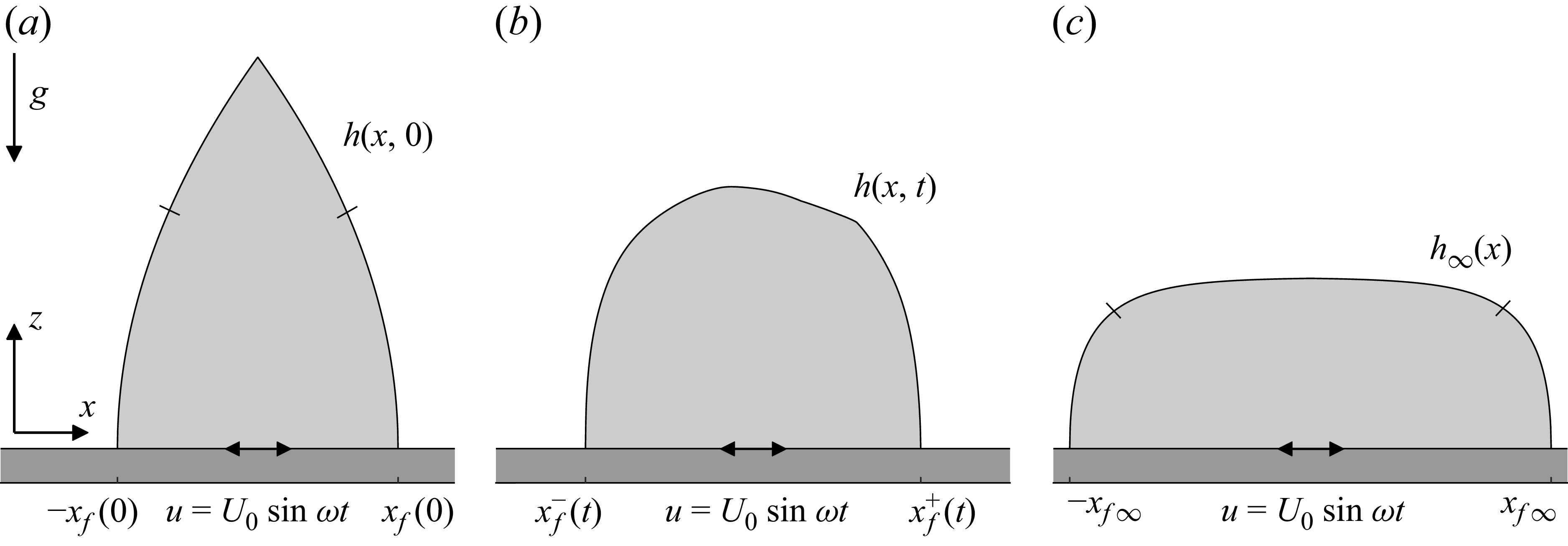


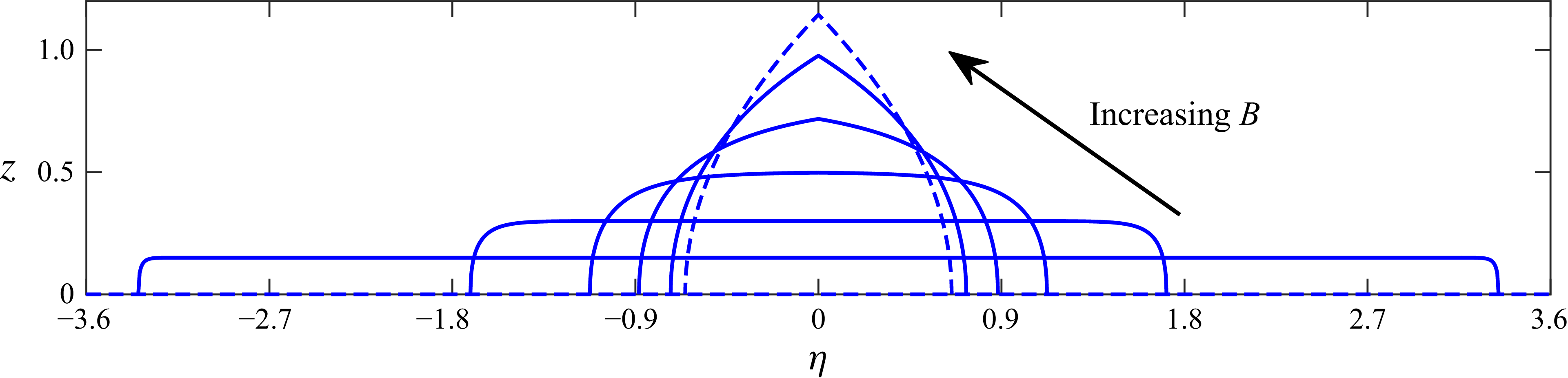


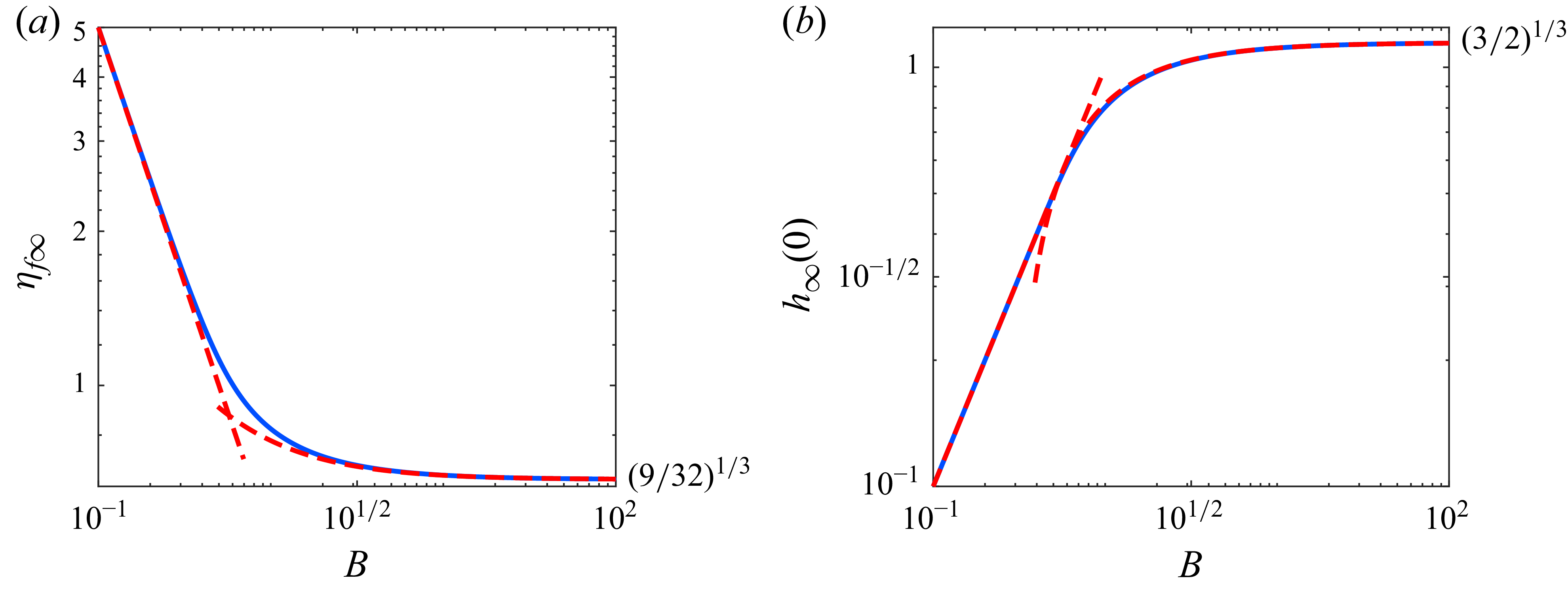


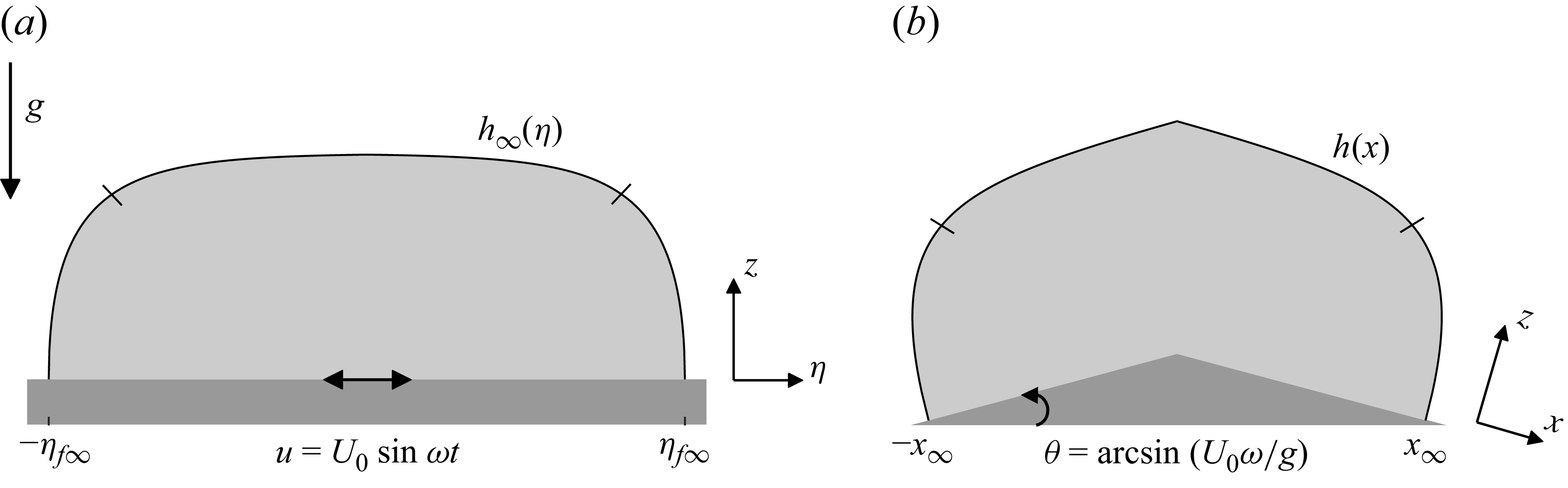


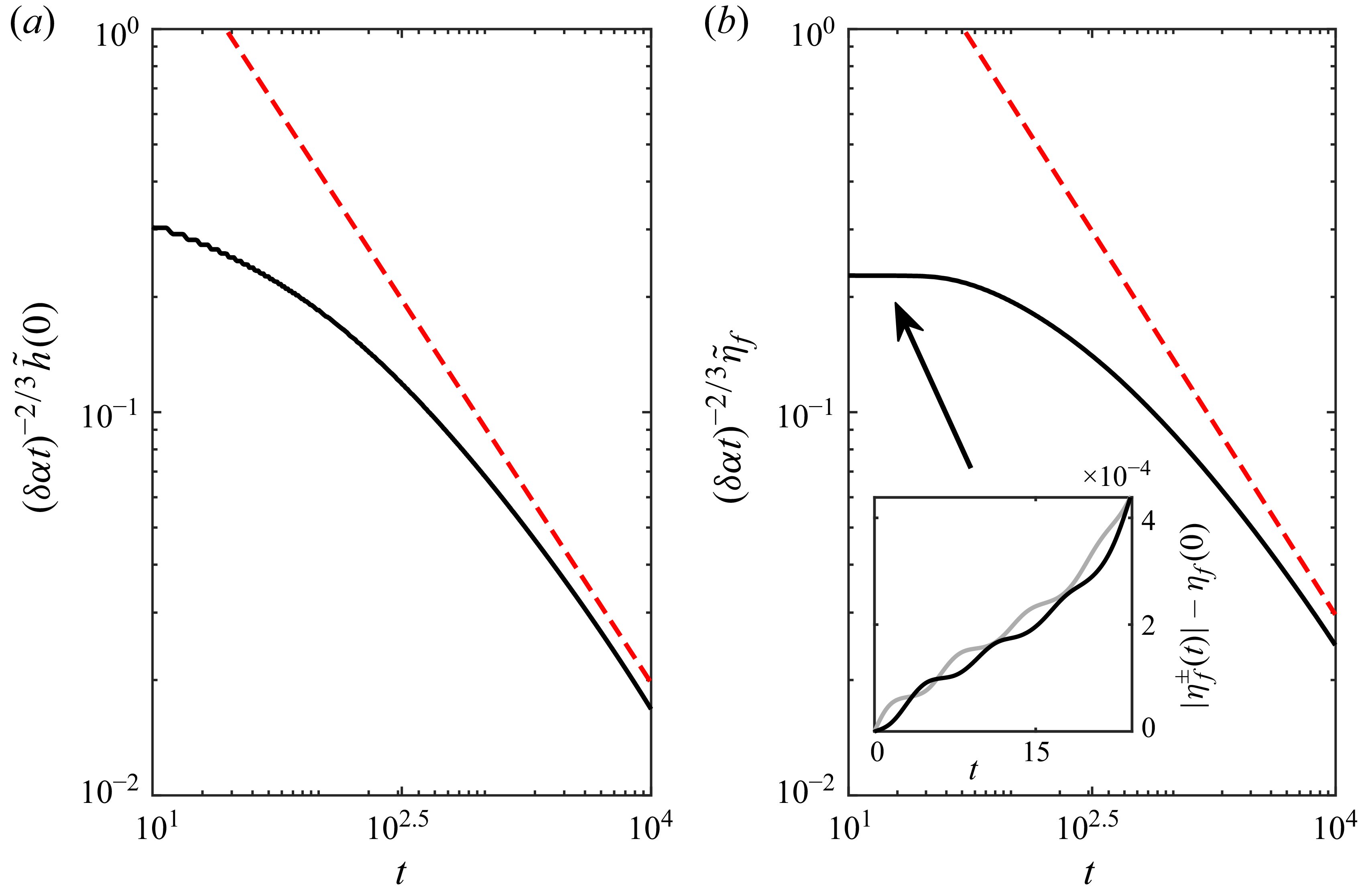


 Open access