


Introduction
Studying past climatic variations to understand the processes that determine plant community composition and resilience to large-scale compositional shifts is central to paleoecology (Tausch et al., Reference Tausch, Wigand and Burkhardt1993; Willis et al., Reference Willis, Bailey, Bhagwat and Birks2010; Birks, Reference Birks2019). North American climate–vegetation relationships from the last glacial maximum (LGM) to the present are well explored (e.g., Bartlein et al., Reference Bartlein, Anderson, Anderson, Edwards, Mock, Thompson, Webb and Whitlock1998; Williams et al., Reference Williams, B. Shuman, Webb, Bartlein and Leduc2004). Longer timescale relationships, such as the conditions during the last interglacial–glacial cycle, are less known but do provide an opportunity to examine multiple examples of vegetation responses to climate shifts, such as those that occur between Marine Oxygen Isotope stages (MIS).
The last interglacial–glacial cycle (MIS 5–2) contains several warm (interstadial) and cold (stadial) periods useful for examining vegetation responses to rapid, global-climate shifts. Climate driven responses of vegetation have been explored using European pollen records (Guiot et al., Reference Guiot, de Beaulieu, Cheddadi, David, Ponel and Reille1993; Cheddadi et al., Reference Cheddadi, de Beaulieu, Jouzel, Andrieu-Ponel, Laurent, Reille, Raynaud and Bar-Hen2005, Lucchi, Reference Lucchi2008; Jiménez-Moreno et al., Reference Jiménez-Moreno, Fauquette and Suc2010b), and regionally in North America (Glover et al., Reference Glover, George, Heusser and MacDonald2021). Compiling pre-LGM pollen records at continental scales provides both a novel dataset for paleoecological study and for reconstructing vegetation dynamics independent of human influence through multiple climate scenarios between stadial and interstadial periods (Tzedakis et al., Reference Tzedakis, Raynaud, McManus, Berger, Brovkin and Kiefer2009). European records suggest MIS 5e was >4.3℃ warmer than present with higher plant community turnover in Central Europe compared to the north and south (Wohlfarth, Reference Wohlfarth2013; Felde et al., Reference Felde, Flantua, Jenks, Benito, de Beaulieu, Kuneš and Magri2020; Wilcox et al., Reference Wilcox, Honiat, Trüssel, Edwards and Spötl2020). Europe transitioned between warm, forested periods during MIS 5 and cool, open vegetation from MIS 4 through MIS 2 (Helmens, Reference Helmens2014). In North America few syntheses of last interglacial–glacial vegetation changes exist, despite available data (Glover et al., Reference Glover, George, Heusser and MacDonald2021) (Table 1). Around 50 North American pollen records are reported to pre-date the LGM (Williams et al., Reference Williams, Grimm, Blois, Charles, Davis, Goring, Graham, Smith, Anderson and Arroyo-Cabrales2018). Of these, ∼20 have sampling-resolution and age-model constraints that allow for a pre-LGM analysis of continental-scale, temporal and spatial patterns of diversity change. These data are distributed across several North American ecoregions (Fig. 1). Grouping individual sites into broader ecoregions (Bailey, Reference Bailey2014) allows for an ecosystem-centric examination of vegetation dynamics for the past 130 ka.
Map of the 23 sites used in this study. Site locations are shown as circles with the site names. Sites are colored based on the seven regional groupings determined by the DCA (Supplemental Figure 2). The seven DCA regions encompass nine level-I ecoregions. The represented ecoregions are shown in color and listed in the legend. Several of the seven DCA regions represent multiple level ecoregions. Due to the lack of sites in the northeast, the Eastern Temperate Forest is divided into level-II classifications.
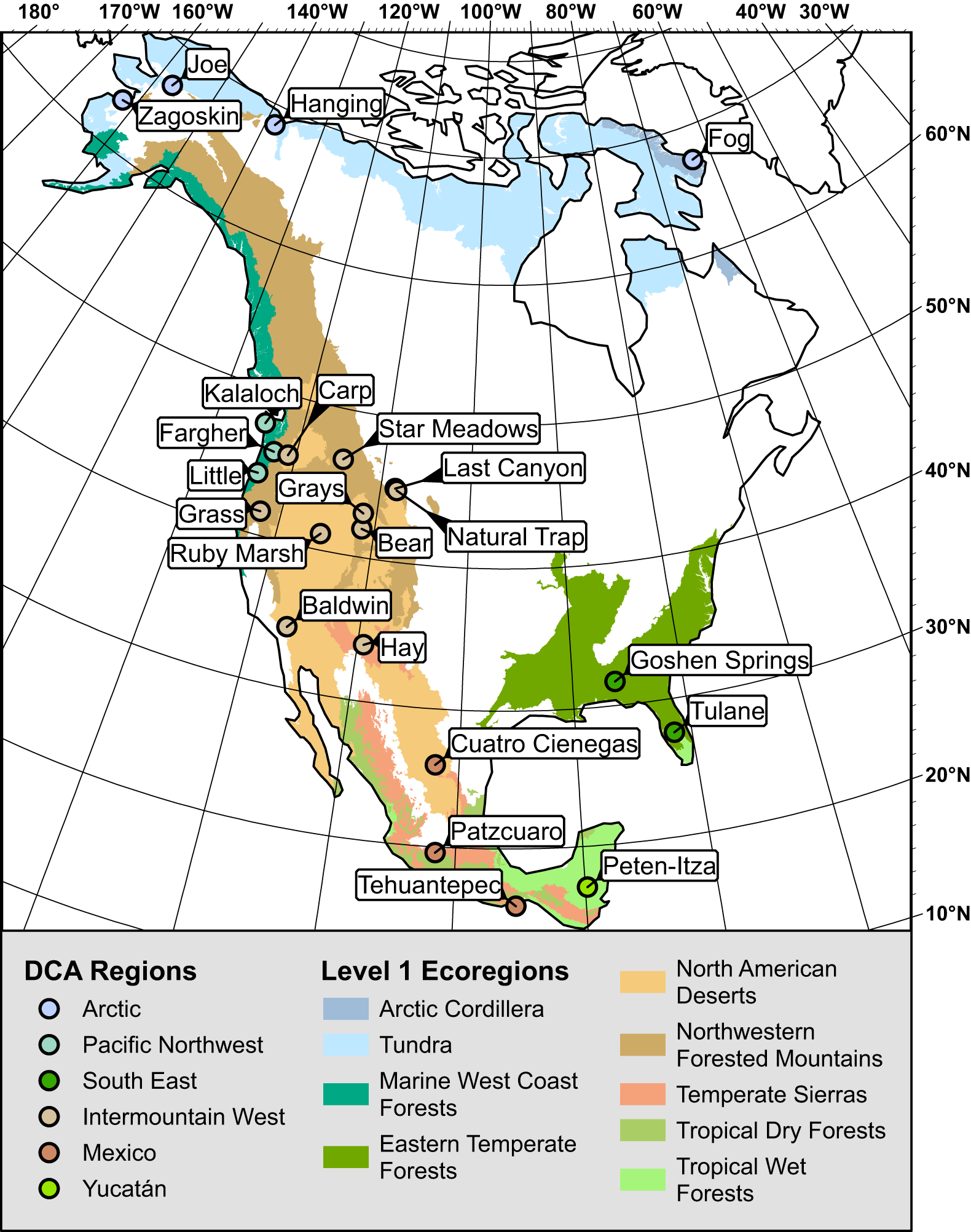
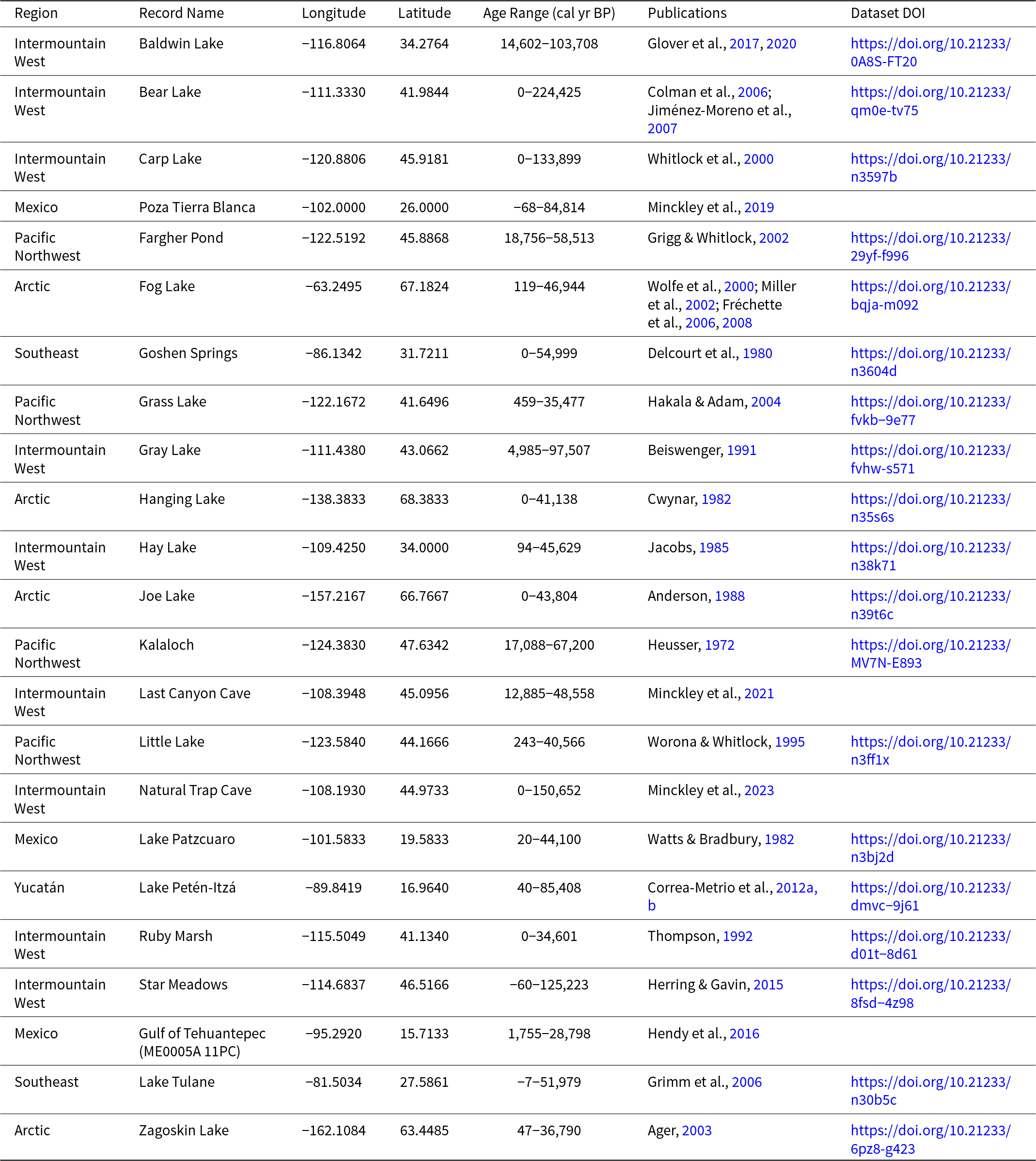
Table of sites used in this study and their associated publications. Age Range calculated as the difference between the youngest date and the oldest. Region includes the DCA-based grouping made in this study.
Plant communities vary along environmental gradients at different spatial and temporal scales (ter Braak and Prentice, Reference ter Braak and Prentice2004). These often appear as elevational and latitudinal gradients that result from underlying temperature and moisture gradients, particularly in mountainous regions (Gentry, Reference Gentry1988; von Humboldt and Bonpland, Reference von Humboldt and Bonpland2010; Lamanna et al., Reference Lamanna, Blonder, Violle, Kraft, Sandel, Šímová and Donoghue2014; Felde et al., Reference Felde, Peglar, Bjune, Grytnes and Birks2016). As environmental gradients shift, the spatial extent of plant communities shift in response (Comes and Kadereit, Reference Comes and Kadereit1998; Thuiller et al., Reference Thuiller, Lavorel, Araújo, Sykes and Prentice2005). Plant communities can be characterized through estimates of taxonomic diversity, incorporating measures of richness (number of taxa) and evenness (distribution of taxa abundances) (Schuler and Gillespie, Reference Schuler and Gillespie2000; Howard and Lee, Reference Howard and Lee2003; Sax and Gaines, Reference Sax and Gaines2003). Studies show high plant diversity maintains ecosystem functions and services including high net primary productivity (NPP) (Tilman et al., Reference Tilman, Lehman and Thomson1997; Hector et al., Reference Hector, Schmid, Beierkuhnlein, Caldeira, Diemer, Dimitrakopoulos and Finn1999; Isbell et al., Reference Isbell, Calcagno, Hector, Connolly, Harpole, Reich and Scherer-Lorenzen2011). High diversity is supported by biotic and abiotic factors that allow for independent regional responses to climate (Zak et al., Reference Zak, Holmes, White, Peacock and Tilman2003; Benton, Reference Benton2009; López-Angulo et al., Reference López-Angulo, Pescador, Sánchez, Luzuriaga, Cavieres and Escudero2020). Understanding how plant communities respond to shifts in climate in addition to the conditions that support high diversity can help predict the effect of current warming on ecosystems as they adapt (Stohlgren et al., Reference Stohlgren, Owen and Lee2000; Suggitt et al., Reference Suggitt, Lister and Thomas2019).
Reconstructions of pollen-based, paleodiversity provide scenarios to study shifts in plant community composition (Birks, Reference Birks2019). Modern pollen-derived taxonomic diversity estimates have effectively captured the structure and composition of vegetation on landscapes at local scales (van der Knaap, Reference van der Knaap2009; Matthias et al., Reference Matthias, Semmler and Giesecke2015; Birks et al., Reference Birks, Felde, Bjune, Grytnes, Seppä and Giesecke2016; Felde et al., Reference Felde, Peglar, Bjune, Grytnes and Birks2016) and, while caution must be taken in interpreting pollen-derived diversity estimates (Weng et al., Reference Weng, Hooghiemstra and Duivenvoorden2006; Goring et al., Reference Goring, Lacourse, Pellatt and Mathewes2013; Väli et al., Reference Väli, Odgaard, Väli and Poska2022), diversity estimates can address questions of diversity change from the trends produced. By reconstructing plant paleodiversity trends across North America, we can interpret both ecosystem diversity and dynamics as they responded to past climate changes.
Paleodiversity has been reconstructed via several common indices, including species richness, Shannon’s index, and Simpson’s index (Morris et al., Reference Morris, Caruso, Buscot, Fischer, Hancock, Maier and Meiners2014). While these methods are still commonly used, other methods such as Hill numbers are more versatile via their ability to vary between different orders (Jost Reference Jost2006, Reference Jost2007). Applying diversity indices in a paleo context can be complicated by several taxonomic-scale-related problems (Cleal et al., Reference Cleal, Pardoe, Berry, Cascales-Miñana, Davis, Diez and Filipova-Marinova2021), such as varying taxonomic resolution (Birks and Birks, Reference Birks and Birks2000) and less information for taxonomic classifications (Godfray et al., Reference Godfray, Knapp, Forey, Fortey, Kenrick and Smith2004). While much of this is simply the nature of working within the fossil record, incorporating plant functional traits can provide a means to reconstruct ecosystem dynamics where taxonomy alone cannot (Eronen et al., Reference Eronen, Polly, Fred, Damuth, Frank, Mosbrugger, Scheidegger, Stenseth and Fortelius2010; Barnosky et al., Reference Barnosky, Hadly, Gonzalez, Head, Polly, Lawing and Eronen2017; Chacón-Labella et al., Reference Chacón-Labella, Hinojo-Hinojo, Bohner, Castorena, Violle, Vandvik and Enquist2023).
In this study, we used pollen-derived taxonomic and functional diversity estimates to quantify North American plant community dynamics from the last interglacial period (MIS 5e) to the present (MIS 1). We hypothesize that global temperature variability and latitudinal temperature gradient compression drove shifts in taxonomic and functional diversity. We examine whether continental and regional shifts in pollen-derived taxonomic diversity are mirrored in functional trait-based diversity for six geographic regions of North America based on 23 fossil pollen records.
Regional Setting
Modern North American ecoregion floristics are represented by high species richness in the tropics of southern Mexico, southeastern United States, and Pacific coast (Ricketts et al., Reference Ricketts, Dinerstein, Olsen, Loucks, Eichbaum, DellaSalla and Kavanagh1999). We can use sub-biome ecoregions (Bailey, Reference Bailey2014) to characterize subcontinental scale regions with similar floristics to scale up from individual sites to broader, floristic heterogeneity at the continental scale. Richness is lowest in the sagebrush steppe and grasslands of the continental interior and Arctic tundra (Cavender-Bares et al., Reference Cavender-Bares, Schweiger, Pinto-Ledezma, Meireles, Cavender-Bares, Gamon and Townsend2020). While plant and pollen diversity are not directly analogous, regional correlations between the two have been established in northern Europe (Reitalu et al., Reference Reitalu, Bjune, Blaus, Giesecke, Helm, Matthias and Peglar2019).
To verify whether North American ecoregions reasonably correspond to the pollen record, we grouped 23 North American pollen records, dated to at least 40 cal ka BP, into six regions based on a detrended correspondence analysis (DCA) of pollen type abundances (Supplemental Figs. 1 and 2). These DCA-based groupings align with level-I ecoregions of North and Central America with 9 of 15 represented (Fig. 1) (CEC, 1997; Griffith et al., Reference Griffith, Omernik and Azevedo1998). DCA clusters grouped similar pollen records based on floristic history rather than modern composition while still being recognizable within modern North American floristics. DCA clusters aligned with ecoregion determinations (CEC, 1997; Griffith et al., Reference Griffith, Omernik and Azevedo1998), which allowed us to use ecoregion changes from present as an interpretive framework (Fig. 1).
Methods
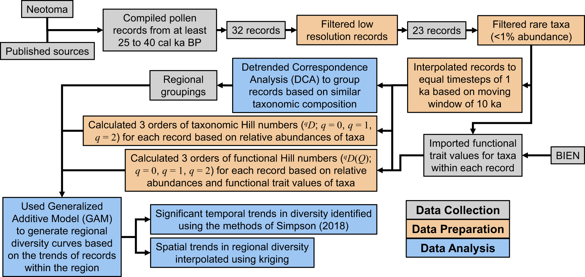
The overall workflow is outlined in Fig. 2 with each step pertaining to one of three categories: data compilation, in which the datasets used were established, data preparation, in which data were transformed and filtered, and data analysis, in which data were used to generate the results presented.
Flowchart of the workflow to generate taxonomic and functional diversity trends for the six regions in this study using publicly available datasets. Steps are colored based on three categories: data collection (gray), where data for the study were accessed; data preparation (orange), where data were filtered and transformed; and data analysis (blue), where the data presented in this study were created.
Records selection
Published pollen data within North America with dated materials to at least 25 cal ka BP and extrapolated to at least 40 cal ka BP were compiled from the Neotoma Paleoecology Database (Williams et al., Reference Williams, Grimm, Blois, Charles, Davis, Goring, Graham, Smith, Anderson and Arroyo-Cabrales2018). Of the 28 records, three were removed for low resolution (fewer than 10 pollen samples or with data spanning less than 10 ka) and six were removed based on constraints in extrapolated age-depth models. Accepted sites also had extrapolations that followed reasonable sedimentation rates based on their 20–30 ka dated intervals. Four newer records not archived in Neotoma at the time of our study were included for a total of 23 records (Table 1). Raw pollen counts were available for all records used in this study.
Data conversions
Pollen taxa identified in each record were filtered based on the level of specificity of the identification. Only terrestrial pollen data were used, excluding spores, aquatic pollen types, and non-pollen palynomorphs to minimize site specific variability (e.g., wetland changes). Pollen taxa with less than 1% abundance in an individual record were excluded. Filtering identified pollen types reduced overall pollen-based, taxonomic richness, but aided in reducing researcher specific biases in pollen identification. The resulting data set contained 142 total pollen types, with 39 family-, 96 genus-, and 7 species-level pollen identifications (Supplemental Table 1).
We interpolated each record to address issues of radiometric dating. Raw pollen counts from each record were converted into relative proportions of the total terrestrial pollen and interpolated using a moving window weighted means interpolation to 1000-year time steps between 0 and 150 ka. Weighted mean interpolations of pollen data were ignored if temporal gaps within the original datasets exceeded ± 5 ka of the centroid of the targeted, 1000-year time step, resulting in discontinuities in our records. Samples within the ± 5 ka window were weighted using a normal curve based on their proximity to the centroid.
DCA and region determination
Similarities of the ecological and taxonomic clustering of the 23 pollen records were verified using DCA, an ordination method appropriate for grouping proportional datasets distributed along broad environmental gradients (Holland, Reference Holland2008; Oksanen et al., Reference Oksanen, Blanchet, Kindt, Legendre, Minchin, O’hara, Simpson, Solymos, Stevens and Wagner2013). DCA was conducted on all samples from all records ensuring that complete histories were considered simultaneously. Other ordination approaches for determining pollen–environment relationships (e.g., canonical correspondence analysis [CCA]) did not improve or enhance our analysis.
Hill numbers
Hill numbers are a family of interrelated diversity estimates that vary by the weights of rare and common taxa and are expressed as ‘effective number of species’ (Chao et al., Reference Chao, Chiu and Jost2014a, Reference Chao, Chiu and Jostb). Hill numbers have proven to be a versatile approach to representing multiple diversity estimates simultaneously (Ohlmann et al., Reference Ohlmann, Miele, Dray, Chalmandrier, O’Connor and Thuiller2019). While commonly used to represent taxonomic diversity, a framework exists for calculating functional diversity with Hill numbers, although it has yet to be adopted in a paleoecological context (Chiu and Chao, Reference Chiu and Chao2014). With taxonomic Hill numbers, the ‘species’ that diversity is calculated from is the relative proportion of the taxa. In functional Hill numbers, the ‘species’ is the functional distance between two taxa rather than the proportions (Chao et al., Reference Chao, Chiu and Jost2014a). Simply, the outputs of taxonomic Hill numbers are in units of ‘effective number of species,’ indicating a value of x is equivalent to x number of equally abundant species within a community. Functional diversity is interpreted as x number of equally abundant and functionally distinct species.
Varying both taxonomic and functional Hill numbers by the variable q adjusts the weights between rare and common taxa or functional distances in an assemblage. Lower q values produce higher diversity estimates through the inclusion of both rare and common taxa/distances while higher q values produce lower estimates by filtering out rare taxa/distances. We calculated three taxonomic and three functional Hill numbers for each sample within a site to model diversity over time within the sites. The taxonomic Hill number of order q (qD) follow formula Equation 1a (Chao et al., Reference Chao, Gotelli, Hsieh, Sander, Ma, Colwell and Ellison2014b):
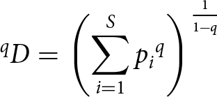 \begin{equation}{}^{q}D = {\left( {\mathop \sum \limits_{i = 1}^S {p_i}^q} \right)^{\frac{1}{{1 - q}}}}\end{equation}
Where S equals the total number of species in the assemblage, pi equals the proportion of species i. To represent functional diversity, Chiu and Chao (Reference Chiu and Chao2014) modified taxonomic Hill numbers (qD) to include the mean functional distance between any two randomly sampled individuals in the assemblage using Rao’s quadratic entropy (Q) as defined by Equation 2 (Rao, Reference Rao1982):
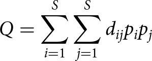 \begin{equation}Q = \mathop \sum \limits_{i = 1}^S \mathop \sum \limits_{j = 1}^S {d_{ij}}{p_i}{p_j}\end{equation}
Where S and pi remain unchanged from Equation 1a, pj equals the proportions of species j, and dij equals the functional distance between species i and j, calculated using Gower distances. Distance measures are calculated between all species but vary in precision based on the number of trait observations. The resulting functional Hill numbers (qD(Q)) are described by Equation 3a (Chiu and Chao, Reference Chiu and Chao2014):
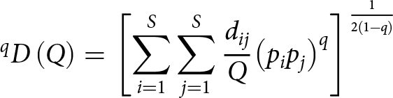 \begin{equation}{}^{q}D\left( Q \right) = {\left[ {\mathop \sum \limits_{i = 1}^S \mathop \sum \limits_{j = 1}^S \frac{{{d_{ij}}}}{Q}{{\left( {{p_i}{p_j}} \right)}^q}} \right]^{\frac{1}{{2\left( {1 - q} \right)}}}}\end{equation}
Where all variables are the same as defined in Equations 1a and 2. When q = 1 in either metric, the equations are undefined and Equations 1b and 3b, which are equivalent to the limit as q approaches 1, must be used for taxonomic and functional diversity, respectively:
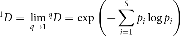 \begin{equation}{}^{1}D = \,\mathop {\lim }\limits_{q \to 1} {}^{q}D = {\text{exp}}\left( { - \mathop \sum \limits_{i = 1}^S {p_i}\log {p_i}} \right)\end{equation}
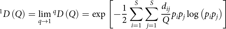 \begin{equation}{}^{1}D\left( Q \right) = \mathop {\lim }\limits_{q \to 1} {}^{q}D\left( Q \right) = {\text{exp}}\left[ { - \frac{1}{2}\mathop \sum \limits_{i = 1}^S \mathop \sum \limits_{j = 1}^S \frac{{{d_{ij}}}}{Q}{p_i}{p_j}\log \left( {{p_i}{p_j}} \right)} \right]\end{equation}
The first three orders of taxonomic diversity collapse down to three common indices: Richness (0D), Shannon’s index (1D), and Simpson’s index (2D). These indices weight all species equally, all species by their relative abundance, and all species by the square of their relative abundance, respectively. For functional diversity, 0D(Q) and 2D(Q) correspond to functional attribute diversity (FAD) and Gini–Simpson index. 1D(Q) does not correspond to an existing index, but for naming consistency we refer to it as functional Shannon’s index, although it is important to reiterate the two are not directly equivalent (Chiu and Chao, Reference Chiu and Chao2014). 0D(Q) can be thought of as the sum of all functional distances, 1D(Q) as the sum of all functional distances weighted by their relative abundance, and 2D(Q) as the sum of all functional distances weighted by the square of their relative abundance.
Seven traits were selected for functional diversity analysis: leaf mass per area, leaf lifespan, max plant height, max plant longevity, seed mass, whole plant growth form, and whole plant woodiness. We selected these traits due to their abundant number of observations and ability to represent most plant ecological strategies through the leaf-height-seed scheme (Westoby, Reference Westoby1998). Some traits are auto-correlated (e.g., leaf lifespan and leaf mass per area), affecting dij and Q, which in turn alter the magnitude of functional diversity values, but not the overall pattern, which is driven by pi and pj.
Trait data were compiled following Brussel and Brewer (Reference Brussel and Brewer2021), using the Botanical Information and Ecology Network (BIEN) database and filtered to include only North and Central America taxa (Maitner et al., Reference Maitner, Boyle, Casler, Condit, Donoghue, Durán and Guaderrama2018). For species-level pollen-types, trait values for all occurrences were averaged and reported. For genus- or family-level pollen types, we averaged the values of all species in those groupings and used the averages as the trait value for the taxon. Families and genera containing species with multiple growth forms (herbaceous and woody taxa) were treated as a different category from woody or herbaceous taxa when calculating functional diversity. To quantify the uncertainty associated with using trait averages, we performed a Monte Carlo simulation. Trait values were resampled to create simulated distributions of 5000 values from which we calculated the mean. This was repeated 10,000 times, creating a distribution of 10,000 means per trait, from which we sampled 100 means and calculated the associated functional diversity estimates.
Distances are calculated from the trait values of each species compared pairwise with all other species in the assemblage. This method is effective in cases when all taxa within an assemblage are identified to the species level and there is little variation in trait values (Pérez-Harguindeguy et al., Reference Pérez-Harguindeguy, Díaz, Garnier, Lavorel, Poorter, Jaureguiberry and Bret-Harte2016). Complications arise when taxa within an assemblage are identified at genus or family levels and there is higher variation in trait values. Averaged trait values ignore the natural variability that exists within a genus or family (Roscher et al., Reference Roscher, Schumacher, Gubsch, Lipowsky, Weigelt, Buchmann, Schulze and Schmid2018; Sotomayor et al., Reference Sotomayor, Hampel, Vázquez, Forio and Goethals2022). However, our goal is to use traits to group pollen (plants) independently of their underlying taxonomy rather than use traits for their functional interpretations. The resulting functional diversity estimate loses the ability to draw specific environmental interpretations but provides comparator diversity datasets to analyze along with taxonomic diversity data.
Temporal analysis
Regional diversity trends were interpolated using a generalized additive model (GAM) to smooth the individual trends of each site within a region. The GAM model was calculated using the ‘gam’ function within the mgcv package in R Studio (Wood, Reference Wood2001). Age was used as the predictor and diversity as the response with a Gaussian family, a normal/identity link function, and a restricted maximum likelihood (REML) smoothing method. Records within each region vary in length, affecting the GAM smoother and decreasing individual site influence towards the present. We selected a GAM to allow for the identification of significant shifts in the diversity time series based on the methods outlined in Simpson (Reference Simpson2018). Times of significant change were highlighted on the splines. Site diversity values were normalized around the mean to enable comparisons of shift magnitude between regions and to highlight differences between the temporal patterns of the taxonomic and functional metrics. Without normalization, questions of the validity of diversity estimate values could prevent thorough interrogations of the trends being presented. Raw diversity trends are shown in Fig 6 and Supplemental Figs 3, 4, and 5. GAM splines are plotted alongside regional temperature records (δ18O) and atmospheric CO2.
Spatial analysis
For each region, we calculated the average of non-transformed taxonomic and functional diversity of each MIS. We then interpolated average diversity using empirical Bayesian kriging, chosen for its ability to quantify standard error and assumption of spatial correlation between inputs (Krivoruchko, Reference Krivoruchko2012). Resulting maps use a bivariate color scale in which high values in both taxonomic and functional diversity are displayed in blue and high values in either taxonomic or functional diversity are displayed in black or orange, respectively. Results for each region are mapped to indicate the distribution of and change in diversity between MISs.
Results
Regionalization of records
Pollen records were grouped into six North American ecoregions: the Arctic (4 sites), Pacific Northwest (3 sites), Intermountain West (10 sites), the Southeast (2 sites), Mexico (3 sites), and Yucatán (1 site). The Yucatán site was an outlier in the DCA (Supplemental Figs. 1 and 2). The floristic composition of the Yucatán record is primarily tropical taxa, distinguishing it from all other records.
Temporal diversity trends
Monte Carlo simulations show minimal variation in the magnitude and no variation in the trend of functional diversity, indicating the estimates do not vary significantly with uncertainty in trait averages. We found trends for richness (0D) and FAD (0D(Q)) to be distinct from the trends for Shannon’s (1D) and functional Shannon’s indices (1D(Q)) and Simpson’s (2D) and Gini–Simpson’s indices (2D(Q)), while the trends of the latter two are similar. Richness and FAD are distinct from the other two orders because of its exclusion of abundance (Fig. 3). In most cases, trends for Simpson’s and Gini Simpson’s indices have steeper increases and decreases, appearing as Shannon’s and functional Shannon’s indices trends with higher amplitude (Figs. 4 and 5). In all three orders of q, diversity trends differ by region. Although continental-scale patterns of diversity change are not apparent, regional diversity show examples of long-term trends and the influence of stadial and interstadial periods.
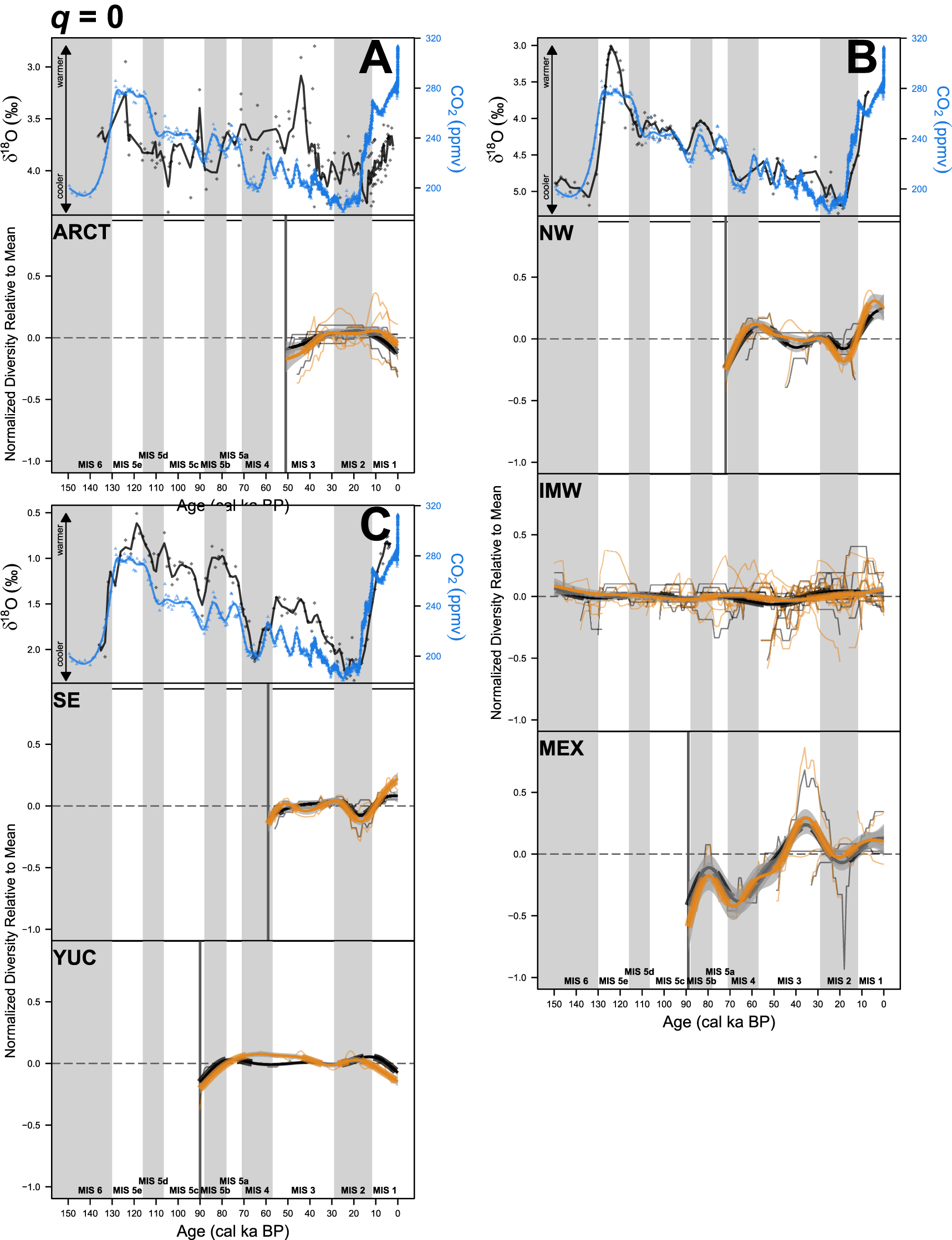
Normalized regional plant diversity of order q = 0 time series with climate. (A) Oxygen isotope record for the Arctic (Cronin et al., Reference Cronin, Keller, Farmer, Schaller, O’Regan, Poirier, Coxall, Dwyer, Bauch and Kindstedt2019) with arctic (ARCT) regional plant diversity. (B) Oxygen isotope record the Eastern Pacific Ocean (Herbert et al., Reference Herbert, Schuffert, Andreasen, Heusser, Lyle, Mix, Ravelo, Stott and Herguera2001) with Pacific Northwest (NW), Intermountain West (IMW), and Mexico (MEX) regional plant diversity. (C) Oxygen isotope record for the Caribbean (Schmidt et al., Reference Schmidt, Spero and Lea2004) with Southeast (SE) and Yucatán (YUC) regional plant diversity. Global atmospheric CO2 concentration from the EPICA Dome ice core (Bereiter et al., Reference Bereiter, Eggleston, Schmitt, Nehrbass-Ahles, Stocker, Fischer, Kipfstuhl and Chappellaz2015) is plotted in all climate plots in blue. Taxonomic richness (0D) is shown in black. Functional attribute diversity (FAD; 0D(Q)) is shown in orange. Individual site trends are plotted as thin lines. Gray vertical bars represent stadial (cool) MIS and white bars represent interstadial (warm) MIS (Lisiecki and Raymo, Reference Lisiecki and Raymo2005). The dotted line at y = 0 indicates the mean of each site following normalization. Bold lines represent GAM splines displaying the interpolated diversity of order q = 0 trends for each region with the 95% confidence interval shaded. Thickened segments of the spline indicate sections of significant slope.
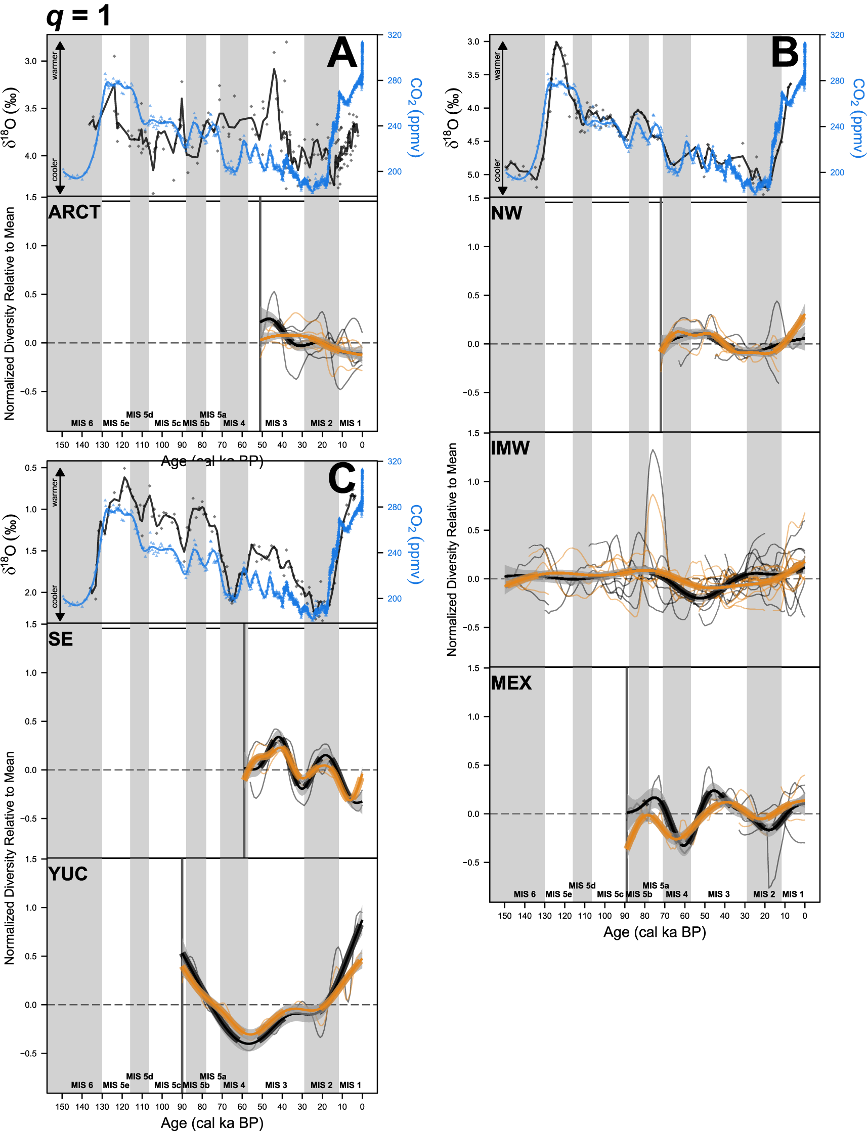
Normalized regional plant diversity of order q = 1 time series with climate following the format of Fig 3. Shannon’s index (1D) is shown in black. Functional Shannon’s index (1D(Q)) is shown in orange. ARCT = Arctic; NW = Pacific Northwest; IMW = Intermountain West; MEX = Mexico; SE = Southeast; YUC = Yucatán.
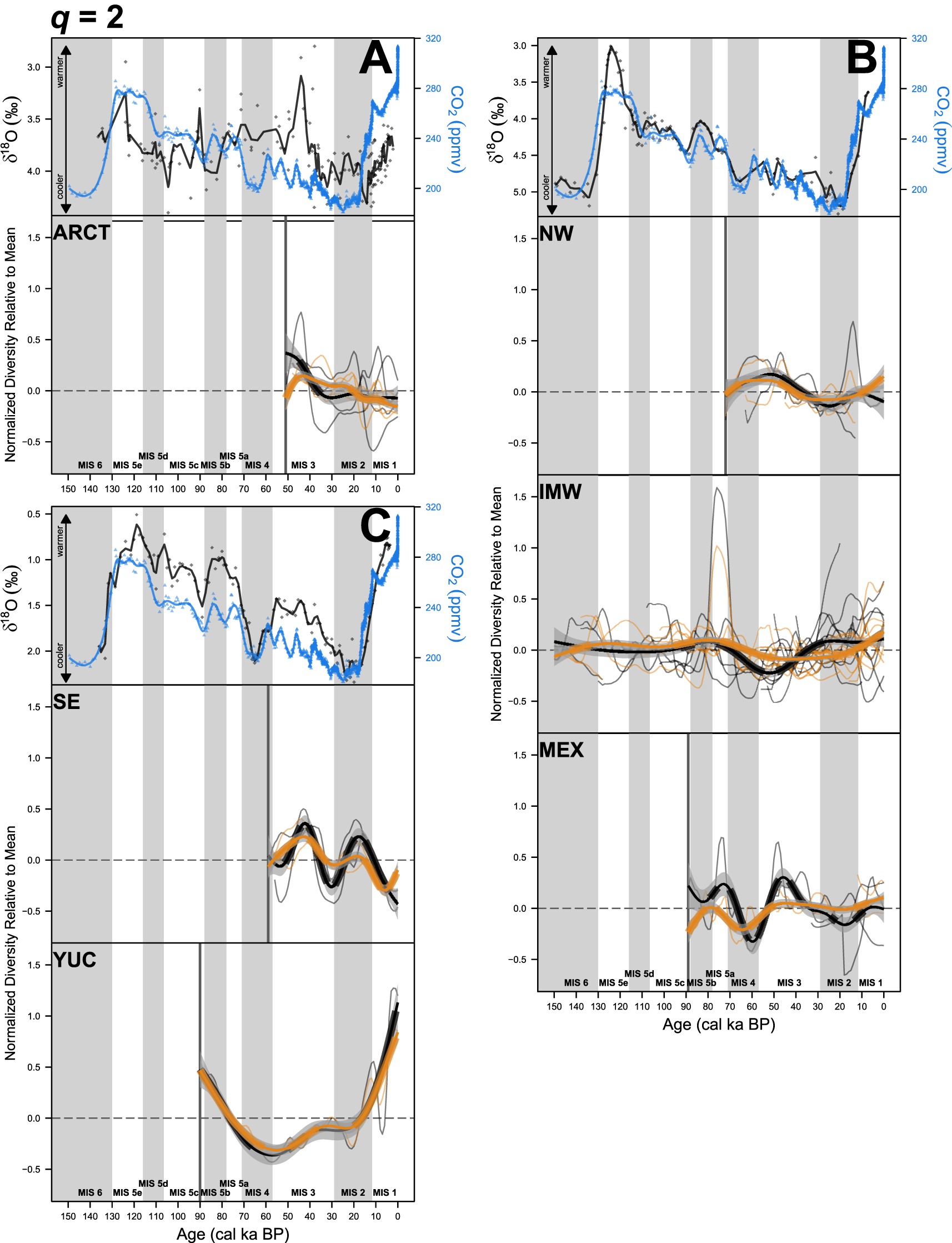
Normalized regional plant diversity of order q = 2 time series with climate following the format of Fig 3. Simpson’s index (2D) is shown in black. Gini–Simpson’s index (2D(Q)) is shown in orange. ARCT = Arctic; NW = Pacific Northwest; IMW = Intermountain West; MEX = Mexico; SE = Southeast; YUC = Yucatán.
Richness (0D) and FAD (0D(Q)) trends follow each other well with significant shifts in one commonly reflected in the other. Both metrics remains stable around the mean in all regions except Mexico. Richness trends in Mexico show relative increases, with below average richness at the beginning of the record and average richness by the end. All other regions fluctuate around the mean but do not exhibit long-term shifts in magnitude. Richness and FAD vary inconsistently from global temperature as represented by atmospheric CO2 with regions responding independently and within region responses being unpredictable during stadial and interstadial conditions. Regional climate records align more closely with richness and FAD however there remains are large degree of variance in response to shifts in regional climate.
Shannon’s (1D) and functional Shannon’s indices (1D(Q)) trends are similar showing less stability around the mean than richness and FAD. Multiple regions fluctuate around the mean (e.g., Arctic, Pacific Northwest, Intermountain West, and Mexico), while others decrease (e.g., Southeast) or experience large shifts in diversity (e.g., Yucatán). Shannon’s and functional Shannon’s indices follow similar patterns to richness and FAD when compared with the regional climate records and atmospheric CO2. However, shifts in regional climate correspond more consistently with shifts in the Shannon’s and functional Shannon’s indices than with richness and FAD.
Simpson’s (2D) and Gini–Simpson’s indices (2D(Q)) trends again follow each other at a similar level to Shannon’s and functional Shannon’s indices. However, the two metrics mismatch to a higher degree in Mexico and the Arctic. Within these two regions, Gini–Simpson’s index (2D(Q)) still has the same general pattern as Simpson’s index (2D), but there are differences in magnitude and timing of the shifts within the patterns. Simpson’s and Gini–Simpson’s indices show nearly identical patterns of diversity shifts as Shannon’s and functional Shannon’s indices, differing only in magnitude, mirroring the atmospheric CO2 and regional climate patterns previously described.
Geographic diversity distribution
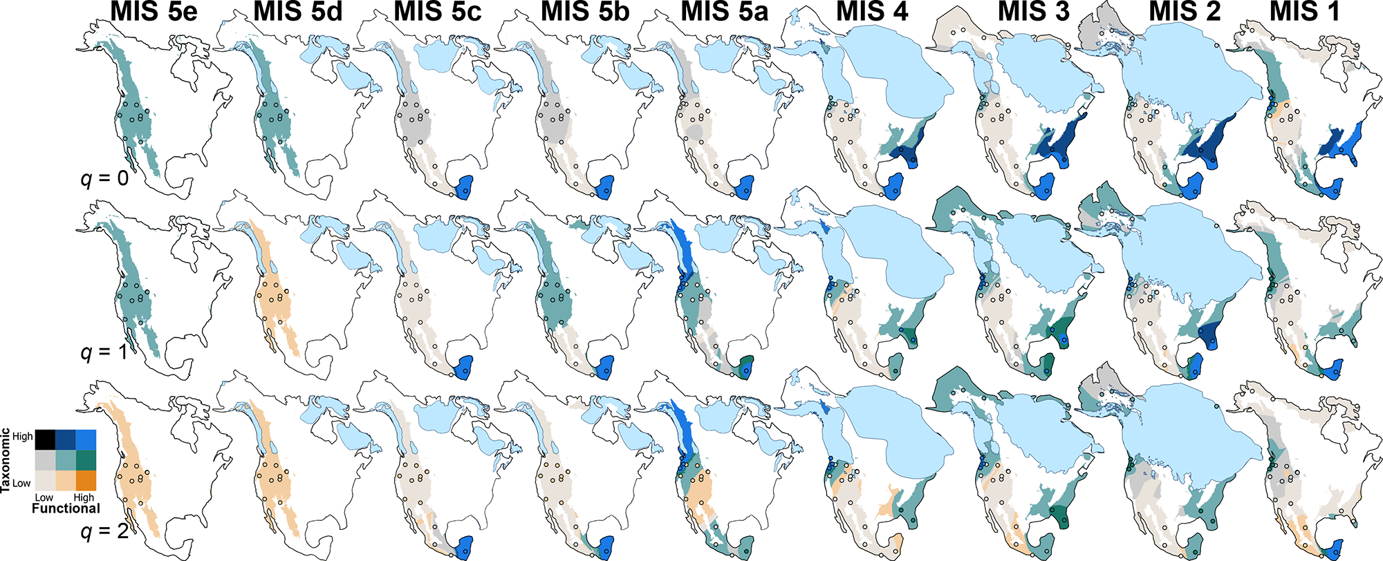
Taxonomic (qD) and functional diversity (qD(Q)) align in terms of the geographic distribution of high and low regional diversity (Fig. 6). However, anticipated continental gradients from low- to high-diversity regions are not consistent between the two metrics (e.g., Lamanna et al., Reference Lamanna, Blonder, Violle, Kraft, Sandel, Šímová and Donoghue2014). Variation in the spatial extent of low taxonomic or functional diversity was not consistent continent-wide. Overall, eastern paleoecological records indicate higher taxonomic pollen diversity compared to western North America. North–south patterns show the Yucatán Peninsula exhibiting the highest diversity in all three orders of q. Prior to MIS 2, the Pacific Northwest shows similarly high diversity to the Yucatán followed by the Southeast. These patterns of taxonomic pollen diversity are generally captured by the functional metrics with variance in the magnitude of functional diversity relative to taxonomic diversity.
Bivariate maps of the geographic distribution of plant diversity in North America. Taxonomic diversity is indicated by the gray shading while functional diversity is orange shading. High values are indicated by dark shading and low values by light shading. Blue shading indicates overlap between taxonomic and functional diversity. Site locations are indicated by points colored by interpolation input values. Mismatches between site color and interpolated diversity are due to a combination of interpolation, including diversity of adjacent regions and the rounding of values. Ecoregions lacking data are overlain in white. Color schemes for both taxonomic and functional diversity are geometrically scaled (color intervals are based off a geometric series). Taxonomic richness (0D) is scaled from |minimum value – 17.9|17.9 – 24.6|24.6 – maximum value|. Functional attribute diversity (0D(Q)) is scaled from |minimum value – 25.2|25.2 – 34.0|34.0 – maximum value|. Shannon’s index (1D) is scaled from |minimum value – 4.8|4.8 – 6.6|6.6 – maximum value|. Functional Shannon’s index (1D(Q)) is scaled from |minimum value – 7.3|7.3 – 9.2|9.2 – maximum value|. Simpson’s index (2D) is scaled from |minimum value – 3.3|3.3 – 4.7|4.7 – maximum value|. Gini–Simpson’s index (2D(Q)) is scaled from |minimum value – 5.0|5.0 – 6.0|6.0 – maximum value|. The extent of the Laurentide Ice Sheet is shown in light blue (Batchelor et al., Reference Batchelor, Margold, Krapp, Murton, Dalton, Gibbard, Stokes, Murton and A. Manica2019). Continent coastlines based on the reconstructed sea-level trends from Cutler et al. (Reference Cutler, Edwards, Taylor, Cheng, Adkins, Gallup, Cutler, Burr and Bloom2003).
Discussion
North American plant taxonomic and functional diversity underwent several asynchronous changes in the last ca. 130 ka. We reject our hypothesis that global temperature variability and latitudinal temperature gradient compression drove shifts in taxonomic and functional diversity. Other global mechanisms, such as CO2 variability, also do not appear to be drivers (Figs. 3–5). Changes in moisture flux into North America could explain regional diversity changes through the last interglacial–glacial cycle, but independent region-to-continental precipitation reconstructions are not available for comparison for this time period. Punctuated patterns of cooling and warming over the last 130 ka did not consistently correspond to changes in taxonomic or functional diversity. When significant diversity changes occurred, we note misalignments in the temporal range between taxonomic and functional trends. With few exceptions, the trends for taxonomic pollen and functional diversity are similar, suggesting that these diversity calculations may be interchangeable.
Richness versus diversity
The trends for richness (0D) and FAD (0D(Q)) in each region are generally more stable than the trends for both Shannon’s (1D) and functional Shannon’s indices (1D(Q)) and Simpson’s (2D) and Gini–Simpson’s indices (2D(Q)). Many regions experience periods of significant change in richness and FAD, but significant changes are less frequent and smaller compared to diversity orders of q = 1 and q = 2, likely reflecting low regional species turnover over time. The pattern of significant change is consistent with species introductions and extirpations that require larger environmental shifts to change plant composition (Dakos et al., Reference Dakos, Matthews, Hendry, Levine, Loeuille, Norberg, Nosil, Scheffer and De Meester2019). The assumption of an individualistic response to climate in paleoecological records is critical and implicitly includes other abiotic and biotic interactions, such as soil or competition conditions (Bartlein et al., Reference Bartlein, Prentice and Webb1986; Davis and Shaw, Reference Davis and Shaw2001). While difficult to quantify, it is possible that changes in richness and FAD require larger magnitude environment changes than are required to shift diversity orders of q = 1 and q = 2, particularly on millennial time scales if extirpation and immigration rates are equal. This is specifically true with pollen data where ‘extirpation’ of a pollen type must overcome local presence and potential residual long-distance transport from extra-local populations.
Diversity patterns of the entire community (order of q = 1) and the dominant taxa (order of q = 2) are similar, indicating diversity shifts are occurring evenly throughout different floristic communities. Compared to richness (0D) and FAD (0D(Q)), Shannon’s (1D), functional Shannon’s (1D(Q)), Simpson’s (2D), and Gini–Simpson’s (2D(Q)) indices all experience higher degrees of diversity fluctuations (Figs. 3–5). These fluctuations indicate regional community composition varies while large species turnover is uncommon as indicated by the richness stability. Shifts in richness indicate extirpation and immigration as species ranges change. Our results show that the composition of floristic communities across the continent have been pliable in response to regional climate change.
Taxonomic versus functional diversity
Taxonomic and functional diversity trends are similar over the last ca. 130 ka, indicating paired analysis is not necessary if taxonomic or functional data are available. The two metrics differ in two key ways: when significant shifts occur in the time-series and the amplitude of trends. The use of Hill numbers allows us to be confident that similarities and differences between the metrics are a result of data differences and not an artifact of the selected indices. Differences between the two metrics could be due to shifts in the dominant plant functional types without corresponding shifts to the actual taxa present in these ecosystems (Doxa et al., Reference Doxa, Devictor, Baumel, Pavon, Medail and Leriche2020). For example, it’s possible that with expansion of the Laurentide Ice Sheet, the southward displacement of conifers shifted the functional diversity in many regions that were previously dominant in broad-leaved trees (Williams et al., Reference Williams, B. Shuman, Webb, Bartlein and Leduc2004).
Both taxonomic (qD) and functional (qD(Q)) metrics follow similar temporal and spatial patterns (Figs. 3–6), with both metrics capturing similar patterns of plant diversity across the continent. The similar overall patterns point to taxonomic and functional diversity being inherently linked. Ecosystems are high or low in both metrics with mismatches uncommon (Fig. 6). Similarities between the two metrics show reconstructions of high taxonomic diversity can be considered as productive ecosystems without the need for functional diversity reconstructions. Some communities may experience a large turnover in the species pool with a limited effect on the functional diversity (e.g., Arctic q = 2 – MIS 3) (Villéger et al., Reference Villéger, Miranda, Hernández and Mouillot2010; Ibsen et al., Reference Ibsen, Borowy, Rochford, Swan and Jenerette2020). In the context of climate change, shifts in ecosystem services as characterized by functional diversity are linked to shifts in taxonomic diversity but triggered differently. Functional diversity experienced fewer significant diversity shifts than taxonomic diversity, highlighting the possibility of increased resilience to environmental change. Functional diversity shifts occur both prior to and following species composition shifts, suggesting uncertainty in predicting responses to future climate change. As with taxonomic diversity, regional history plays the most important role in determining the degree to which functional diversity, and by extension ecosystem services, may be affected by climate change.
Regional climate
We expected diversity to increase with distance from the continental ice sheets based on compression of latitudinal temperature gradients. Changes in expected diversity should reflect admixtures of regional floras as they responded to shifts in temperature based on individualistic response of taxa to climate (Bartlein et al., Reference Bartlein, Prentice and Webb1986; Minckley et al., Reference Minckley, Felstead and Gonzalez2019). However, our results show regional responses to global temperature changes are difficult to predict due to mismatches between regional and global climate variability. Significant shifts happened since the last interglacial, but not proximal to MIS boundaries (Figs. 3–5). Age uncertainties and sampling resolution of older pollen records may create enough error in these records to blur direct mechanistic links between MIS transitions and regional vegetation changes. Previous studies have shown vegetation composition to reliably track climate at millennial scales (Harrison and Sanchez Goñi, Reference Harrison and Sanchez Goñi2010; Jiménez-Moreno et al., Reference Jiménez-Moreno, Anderson, Desprat, Grigg, Grimm, Heusser, Jacobs, López-Martínez, Whitlock and Willard2010a), but our results suggest major floral transitions represented by significant changes to pollen diversity lack a direct association with global climate shifts. This discrepancy is likely due to our incorporation of diversity metrics (qD and qD(Q)) rather than focusing on dominant plant taxa. However, describing how correlated the two are to one another will be important for future studies. Regionally, changes in diversity are not uniform in magnitude or trend. In many cases, shifts observed in one region are not paralleled in the trends of another, even when geographically adjacent.
Understanding the role regional climate plays in influencing plant diversity has important implications for how we predict future diversity trends. The regional variability of diversity shifts is one of the difficulties revealed by our study. Plant diversity metrics (qD and qD(Q)) for the Intermountain West indicate a high degree of stability over the last ca. 130 ka. Individual sites within the region experienced transitions between more open sagebrush steppe and closed spruce–fir forests in line with changes from warm–dry to cool–wet climates (Beiswenger, Reference Beiswenger1991; Herring and Gavin, Reference Herring and Gavin2015). Despite changes to its’ floral composition, the overall diversity of the Intermountain West remains relatively low compared to the rest of the continent, indicating that observed compositional shifts are relatively minor compared to more palynologically diverse regions (Fig. 6).
In contrast, the Yucatán, a diversity hotspot for North America, fluctuates more in trend with orders of q = 1 and q = 2 (Figs. 3–5). While the lower diversity of the Intermountain West is partially a result of the biases of the pollen record with family-level pollen types (e.g., Poaceae, Asteraceae, Amaranthaceae) more common in the West than genus-level pollen types (e.g., Betula, Tilia, Acer, etc.) identified in eastern North American pollen records (Qian, Reference Qian1998; Pinto-Ledezma et al., Reference Pinto-Ledezma, Larkin and Cavender-Bares2018; Cavender-Bares et al., Reference Cavender-Bares, Schweiger, Pinto-Ledezma, Meireles, Cavender-Bares, Gamon and Townsend2020). With the flora of the Intermountain West adapted to grow in both hot and freezing arid conditions, changes to the temperature of the environment may not have been severe enough to shift the overall communities, but rather altered the latitudes and elevations that different communities could grow (Breshears et al., Reference Breshears, Huxman, Adams, Zou and Davison2008; Lavin et al., Reference Lavin, Brummer, Quire, Maxwell and Rew2013).
Diversity may tend to decrease into stadial periods and increase into interstadials, but this pattern is not universal (e.g., Mexico q = 1 – MIS 4–2). With the range of environmental conditions contained within the seven North American regions, it is difficult to determine external forcings outside of increased uniformity in hemispheric climate, possibly because of maritime effects. As with global temperature and atmospheric CO2, regional temperature (δ18O) alone does not explain all observed diversity shifts. Many instances exist where diversity increases with increasing temperature (e.g., Southeast q = 0 – MIS 2–1, Yucatán q = 1 – MIS 2–1, Mexico q = 0 – MIS 4–3) and decrease with decreasing temperature (e.g., Pacific Northwest q = 0 – MIS 3–2, Yucatán q = 1 – MIS 5a–4, Mexico q = 0 – MIS 3–2). Mismatches between both conditions occur, with scenarios of increasing diversity with decreasing temperature (e.g., Arctic q = 0 – MIS 3, Southeast q = 1 – MIS 2, Pacific Northwest q = 0 – MIS 4) and decreasing diversity with increasing temperature (e.g., Arctic q = 0 – MIS 2–1, Southeast q = 1 – MIS 2–1, Intermountain West q = 0 – MIS 4–3). While cooler temperatures do not correlate to lower diversity and vice versa (Scheiner and Rey-Benayas, Reference Scheiner and Rey-Benayas1994; Donoghue, Reference Donoghue2008), the lack of clear patterns determining whether a decrease in temperature is associated with a diversity increase, decrease, or no change suggests other climatic factors play a major role. The most likely factor is moisture availability as it is an important environmental gradient for global plant niches (Silvertown, Reference Silvertown2004). However, highly resolved paleohydrology records older than the last glacial period are not readily available, making explorations of this driver of past diversity for North America not currently possible. Regional temperature records align with plant diversity shifts to a better degree than global temperature, but again, without independent moisture data, continental diversity patterns cannot be fully explained. Increased research focusing on isotopic biomarkers (Seki et al., Reference Seki, Meyers, Yamamoto, Kawamura, Nakatsuka, Zhou and Zheng2011; Feakins et al., Reference Feakins, Bentley, Salinas, Shenkin, Blonder, Goldsmith and Ponton2016; Strobel et al., Reference Strobel, Bliedtner, Carr, Struck, du Plessis, Glaser and Meadows2022) could result in the development of regionalized moisture records and complete the picture of regional climates during the last interglacial–glacial cycle.
Conclusions
The reconstructions of geographic and temporal shifts in plant diversity outline the continental dynamics of vegetation over the last ∼130 ka. We examined changes in floristic diversity of the past 130 ka (MIS 5e–MIS 1) using 23 pollen records from North America via the implementation of Hill numbers, allowing for a simultaneous examination of species richness and FAD based on presence-absence (orders of q = 0), rarity (orders of q = 1), or dominance (orders of q = 2). Both Shannon’s (1D) and functional Shannon’s indices (1D(Q)) and Simpson’s (2D) and Gini–Simpson’s indices (2D(Q)) fluctuate to a higher degree than richness (0D) and FAD (0D(Q)), indicating that the compositions within ecosystems were highly variable across the record, while species pools remained relatively constant.
The incorporation of functional diversity (qD(Q)) alongside taxonomic diversity (qD) supported our interpretations of diversity dynamics during the last interglacial–glacial cycle and shows the connectivity between the two metrics. However, desynchronies between taxonomic and functional diversity shifts point to differences in resilience between species composition and ecosystem function. Continued mechanistic investigations into individual region shifts in both taxonomic and functional plant diversity can identify relationships between global climate and regional vegetation to further understand Quaternary plant dynamics.
Our results highlight the relationship between global temperature, regional climate, ecosystem function, and species composition. While shifts in global temperature may correspond with shifts in the regional climate, how plant diversity and the broader ecosystem respond is unpredictable. However, the integration of both taxonomic and functional diversity into our study emphasizes the inseparability between the two. Scenarios exist in which one metric experiences a shift prior to or without the other, yet both maintain similar temporal and spatial patterns to one another throughout the cooling and warming cycles of the last 130 ka.
Supplementary material
The supplementary material for this article can be found at https://doi.org/10.1017/qua.2024.55
Acknowledgments
We thank the contributors to the Neotoma Paleoecology Database (https://www.neotomadb.org/) and the following data contributors for enabling this compilation to be possible: Thomas Ager, Patricia Anderson, Scott Anderson, Jane Beiswenger, Alexander Correa-Metrio, Les Cwynar, Paul Delcourt, Bianca Frechette, Katherine Glover, Laurie Grigg, Eric Grimm, Barbara Hansen, Katharine Hakala, Erin Herring, Calvin Heusser, Bonnie Fine Jacobs, Gonzalo Jiménez-Moreno, Matthew Kirby, Glen MacDonald, John McAndrews, Robert Thompson, Charles Turton, William Watts, Cathy Whitlock, Marjorie Green Winkler, and Mark Worona. In addition, we thank BIEN (https://bien.nceas.ucsb.edu/bien/) and the hundreds of individuals and herbaria whose trait observations and measurements were used in our functional diversity estimates. We thank the University of Wyoming Roy J. Shlemon Center for Quaternary Studies for providing financial support. We appreciate the anonymous reviewers whose comments helped improve this work. We are grateful for the contributions of Simon Brewer, providing code and recommendations in our analyses. Map generation for Figs. 1 and 6 was possible with the help of John Lesko.
Data availability statement
Datasets and R code related to this study can be found at: https://github.com/tjterlizzi/NA_diversity.git.
Funding
This work was supported by the Roy J. Shlemon Center for Quaternary Studies at the University of Wyoming. The center had no involvement in the development or execution of the research.


 Open access