
 CO2
CO2





1. Introduction
Carbon capture and storage (CCS) is the process of capturing carbon dioxide ( ${\textrm {CO}}_{2}$
) from industrial sources or the atmosphere and permanently storing it in underground geological formations. CCS is expected to play an important role in the reduction of greenhouse gas emissions as part of the global energy transition (Intergovernmental Panel on Climate Change 2022, p. 24). In particular, it has the potential to address large-scale
${\textrm {CO}}_{2}$
) from industrial sources or the atmosphere and permanently storing it in underground geological formations. CCS is expected to play an important role in the reduction of greenhouse gas emissions as part of the global energy transition (Intergovernmental Panel on Climate Change 2022, p. 24). In particular, it has the potential to address large-scale ${\textrm {CO}}_{2}$
emissions from difficult to decarbonise industries, such as steel and cement, and to enable
${\textrm {CO}}_{2}$
emissions from difficult to decarbonise industries, such as steel and cement, and to enable ${\textrm {CO}}_{2}$
removal from the atmosphere via direct air capture and storage and bioenergy with CCS (International Energy Agency 2020; The Royal Society 2022).
${\textrm {CO}}_{2}$
removal from the atmosphere via direct air capture and storage and bioenergy with CCS (International Energy Agency 2020; The Royal Society 2022).
Carbon storage in deep saline aquifers is achieved by injecting ${\textrm {CO}}_{2}$
into a layer of permeable rock saturated initially with brine and capped above by an impermeable seal rock. Suitable structures are typically at a depth of 1.0–2.5 km below the surface, where
${\textrm {CO}}_{2}$
into a layer of permeable rock saturated initially with brine and capped above by an impermeable seal rock. Suitable structures are typically at a depth of 1.0–2.5 km below the surface, where ${\textrm {CO}}_{2}$
is supercritical at the aquifer temperature and pressure, and tens to hundreds of metres thick (The Royal Society 2022, p. 10). During the initial injection phase, the flow of
${\textrm {CO}}_{2}$
is supercritical at the aquifer temperature and pressure, and tens to hundreds of metres thick (The Royal Society 2022, p. 10). During the initial injection phase, the flow of ${\textrm {CO}}_{2}$
within these structures is determined by pressure gradients associated with the injection process, buoyancy forces associated with the density difference between
${\textrm {CO}}_{2}$
within these structures is determined by pressure gradients associated with the injection process, buoyancy forces associated with the density difference between ${\textrm {CO}}_{2}$
and brine, and by variations in the permeability of the structure on both large (Chadwick, Williams & Falcon-Suarez Reference Chadwick, Williams and Falcon-Suarez2019; Mortimer, Mingotti & Woods Reference Mortimer, Mingotti and Woods2024) and small scales (Benham, Neufeld & Woods Reference Benham, Neufeld and Woods2022). Following injection, the buoyancy of
${\textrm {CO}}_{2}$
and brine, and by variations in the permeability of the structure on both large (Chadwick, Williams & Falcon-Suarez Reference Chadwick, Williams and Falcon-Suarez2019; Mortimer, Mingotti & Woods Reference Mortimer, Mingotti and Woods2024) and small scales (Benham, Neufeld & Woods Reference Benham, Neufeld and Woods2022). Following injection, the buoyancy of ${\textrm {CO}}_{2}$
leads the plume to travel up-dip towards the highest point in the formation where it becomes structurally trapped by the seal rock. As the plume migrates, a fraction of the injected
${\textrm {CO}}_{2}$
leads the plume to travel up-dip towards the highest point in the formation where it becomes structurally trapped by the seal rock. As the plume migrates, a fraction of the injected ${\textrm {CO}}_{2}$
remains trapped in place by capillary forces as the ambient fluid reinvades the pore spaces (Hesse, Orr & Tchelepi Reference Hesse, Orr and Tchelepi2008). Over long time scales (tens to thousands of years),
${\textrm {CO}}_{2}$
remains trapped in place by capillary forces as the ambient fluid reinvades the pore spaces (Hesse, Orr & Tchelepi Reference Hesse, Orr and Tchelepi2008). Over long time scales (tens to thousands of years), ${\textrm {CO}}_{2}$
dissolves in brine and may eventually precipitate as carbonate minerals, leading to secure and permanent storage (Metz et al. Reference Metz, Davidson, de Coninck, Loos and Meyer2005, p. 208).
${\textrm {CO}}_{2}$
dissolves in brine and may eventually precipitate as carbonate minerals, leading to secure and permanent storage (Metz et al. Reference Metz, Davidson, de Coninck, Loos and Meyer2005, p. 208).
A wide range of analytical and numerical techniques have been applied to model carbon storage in deep saline aquifers and other similar systems of two-phase flow in porous media. One-dimensional depth-averaged models of gravity currents in porous media have formed the basis for many simplified models of ${\textrm {CO}}_{2}$
flow in aquifers. Huppert & Woods (Reference Huppert and Woods1995), Nordbotten & Celia (Reference Nordbotten and Celia2006), and Hesse et al. (Reference Hesse, Tchelepi, Cantwel and Orr2007) derived similarity solutions describing gravity currents resulting from both fixed volume and continuous injection in horizontal reservoirs, and this approach has since been extended to incorporate the effects of capillary trapping and dissolution over long post-injection time scales (Gasda, Nordbotten & Celia Reference Gasda, Nordbotten and Celia2011), aquifers confined by faults (Gunn & Woods Reference Gunn and Woods2011), background flow (Gunn & Woods Reference Gunn and Woods2012), permeability gradients (Hinton & Woods 2018, Reference Hinton and Woods2021), and anisotropic permeability (Benham et al. Reference Benham, Neufeld and Woods2022). Several approaches have also been developed to include the effects of layered aquifer structures into these simplified models. Large-scale (1–10 m or larger) variations, such as aquifers separated by low-permeability mudstone, have been incorporated by considering a coupled system of multiple separate aquifers with the addition of
${\textrm {CO}}_{2}$
flow in aquifers. Huppert & Woods (Reference Huppert and Woods1995), Nordbotten & Celia (Reference Nordbotten and Celia2006), and Hesse et al. (Reference Hesse, Tchelepi, Cantwel and Orr2007) derived similarity solutions describing gravity currents resulting from both fixed volume and continuous injection in horizontal reservoirs, and this approach has since been extended to incorporate the effects of capillary trapping and dissolution over long post-injection time scales (Gasda, Nordbotten & Celia Reference Gasda, Nordbotten and Celia2011), aquifers confined by faults (Gunn & Woods Reference Gunn and Woods2011), background flow (Gunn & Woods Reference Gunn and Woods2012), permeability gradients (Hinton & Woods 2018, Reference Hinton and Woods2021), and anisotropic permeability (Benham et al. Reference Benham, Neufeld and Woods2022). Several approaches have also been developed to include the effects of layered aquifer structures into these simplified models. Large-scale (1–10 m or larger) variations, such as aquifers separated by low-permeability mudstone, have been incorporated by considering a coupled system of multiple separate aquifers with the addition of ${\textrm {CO}}_{2}$
exchange through the mudstone layer (Mortimer et al. Reference Mortimer, Mingotti and Woods2024) and small-scale (1–10 cm) variations, such as layers within an individual aquifer, by determining an effective bulk permeability (Benham, Bickle & Neufeld Reference Benham, Bickle and Neufeld2021).
${\textrm {CO}}_{2}$
exchange through the mudstone layer (Mortimer et al. Reference Mortimer, Mingotti and Woods2024) and small-scale (1–10 cm) variations, such as layers within an individual aquifer, by determining an effective bulk permeability (Benham, Bickle & Neufeld Reference Benham, Bickle and Neufeld2021).
The stability of the interface between two vertically segregated immiscible fluids in porous media was studied by Dietz (Reference Dietz1953). They established that for the two-dimensional flow of oil and water in a reservoir of constant slope, there is a critical flow rate above which the interface cannot be stabilised by gravity, allowing water to bypass the oil by flowing in a thin layer along the lower boundary of the reservoir. Furthermore, Hinton & Jyoti (Reference Hinton and Jyoti2022) applied a linear stability analysis to similarity solutions to show that a Saffman–Taylor instability does not develop at the interface between brine and a vertically segregated plume of ${\textrm {CO}}_{2}$
in an aquifer, even with an arbitrarily small density difference. While one-dimensional reduced-order models have enabled analytical results to be obtained for simplified geometries, larger-scale computational two-dimensional depth-integrated and three-dimensional models have also been used to investigate the flow of
${\textrm {CO}}_{2}$
in an aquifer, even with an arbitrarily small density difference. While one-dimensional reduced-order models have enabled analytical results to be obtained for simplified geometries, larger-scale computational two-dimensional depth-integrated and three-dimensional models have also been used to investigate the flow of ${\textrm {CO}}_{2}$
plumes in more realistic geometry taken from field data. Bergmo, Grimstad & Lindeberg (Reference Bergmo, Grimstad and Lindeberg2011) used a three-dimensional model to investigate the effects of different well configurations (including multiple injection wells and pressure relief using a brine production well) on the pressure build up during injection and the resulting limitations on
${\textrm {CO}}_{2}$
plumes in more realistic geometry taken from field data. Bergmo, Grimstad & Lindeberg (Reference Bergmo, Grimstad and Lindeberg2011) used a three-dimensional model to investigate the effects of different well configurations (including multiple injection wells and pressure relief using a brine production well) on the pressure build up during injection and the resulting limitations on ${\textrm {CO}}_{2}$
storage capacity in the Johansen and Utsira formations in the North Sea Basin offshore from the west coast of Norway. Furthermore, Gasda et al. (Reference Gasda, Nordbotten and Celia2011) used a two-dimensional vertically integrated model incorporating capillary trapping and dissolution to predict the long-term behaviour of injected
${\textrm {CO}}_{2}$
storage capacity in the Johansen and Utsira formations in the North Sea Basin offshore from the west coast of Norway. Furthermore, Gasda et al. (Reference Gasda, Nordbotten and Celia2011) used a two-dimensional vertically integrated model incorporating capillary trapping and dissolution to predict the long-term behaviour of injected ${\textrm {CO}}_{2}$
in the Johansen formation up to 3000 years after injection. More recently, Luboń (Reference Luboń2021) applied a similar three-dimensional modelling approach to three aquifers in Poland with a focus on determining the optimal placement of a single injection well to maximise the storage efficiency of
${\textrm {CO}}_{2}$
in the Johansen formation up to 3000 years after injection. More recently, Luboń (Reference Luboń2021) applied a similar three-dimensional modelling approach to three aquifers in Poland with a focus on determining the optimal placement of a single injection well to maximise the storage efficiency of ${\textrm {CO}}_{2}$
.
${\textrm {CO}}_{2}$
.
Modelling of CCS in deep saline aquifers has largely focussed on either understanding fundamental physics using one-dimensional models limited to simplified geometry and a single injection well, or applying two- or three-dimensional models to specific real-world geometry where multiple injection wells or more complex flows have been considered. We aim to bridge the gap between these approaches by implementing both a one-dimensional axisymmetric and two-dimensional model with simplified geometry. With these models, we systematically explore how design parameters, in particular the ${\textrm {CO}}_{2}$
injection rate and the number and location of injection wells, impact the fraction of available pore space which can be accessed for
${\textrm {CO}}_{2}$
injection rate and the number and location of injection wells, impact the fraction of available pore space which can be accessed for ${\textrm {CO}}_{2}$
storage prior to the termination of injection owing to either
${\textrm {CO}}_{2}$
storage prior to the termination of injection owing to either ${\textrm {CO}}_{2}$
spilling beyond the boundary of the anticline or the pressure build up within the aquifer reaching the fracture pressure of the seal rock. Through this analysis, we identify a trade-off between the rate of injection and the efficiency of
${\textrm {CO}}_{2}$
spilling beyond the boundary of the anticline or the pressure build up within the aquifer reaching the fracture pressure of the seal rock. Through this analysis, we identify a trade-off between the rate of injection and the efficiency of ${\textrm {CO}}_{2}$
storage and that this depends critically on the number and placement of injection wells.
${\textrm {CO}}_{2}$
storage and that this depends critically on the number and placement of injection wells.
In § 2, we derive a two-dimensional depth-integrated model for the flow of a ${\textrm {CO}}_{2}$
plume injected into a confined aquifer saturated with brine with variable seal-rock geometry and constant thickness and a simplified one-dimensional axisymmetric version of this model. In § 3, we use the axisymmetric version of our model to illustrate the behaviour of an axisymmetric plume from a single injection well at the centre of a dome-shaped anticline structure. We first show a detailed example of the flow of
${\textrm {CO}}_{2}$
plume injected into a confined aquifer saturated with brine with variable seal-rock geometry and constant thickness and a simplified one-dimensional axisymmetric version of this model. In § 3, we use the axisymmetric version of our model to illustrate the behaviour of an axisymmetric plume from a single injection well at the centre of a dome-shaped anticline structure. We first show a detailed example of the flow of ${\textrm {CO}}_{2}$
plumes with high and low injection rates, then systematically vary the injection rate to show the transition between buoyancy- and injection-driven regimes in terms of the fraction of available pore space filled by
${\textrm {CO}}_{2}$
plumes with high and low injection rates, then systematically vary the injection rate to show the transition between buoyancy- and injection-driven regimes in terms of the fraction of available pore space filled by ${\textrm {CO}}_{2}$
and the maximum pressure reached in the aquifer during the injection process. In § 4, we use the full two-dimensional model to demonstrate how the plume shape and pressure throughout the aquifer change when the injected
${\textrm {CO}}_{2}$
and the maximum pressure reached in the aquifer during the injection process. In § 4, we use the full two-dimensional model to demonstrate how the plume shape and pressure throughout the aquifer change when the injected ${\textrm {CO}}_{2}$
flow is distributed over multiple injection wells arranged equally spaced at a fixed radius from the centre of the same anticline where we can no longer assume that the plume is axisymmetric. We show the impact of the number and location of injection wells on the fraction of pore space filled and the pressure in the aquifer. This helps to identify the maximum rate at which
${\textrm {CO}}_{2}$
flow is distributed over multiple injection wells arranged equally spaced at a fixed radius from the centre of the same anticline where we can no longer assume that the plume is axisymmetric. We show the impact of the number and location of injection wells on the fraction of pore space filled and the pressure in the aquifer. This helps to identify the maximum rate at which ${\textrm {CO}}_{2}$
can be safely injected without exceeding a given seal rock fracture pressure. In § 5, we contextualise the dimensionless results presented throughout the paper by including an example of equivalent characteristic scalings for our model corresponding to the Endurance
${\textrm {CO}}_{2}$
can be safely injected without exceeding a given seal rock fracture pressure. In § 5, we contextualise the dimensionless results presented throughout the paper by including an example of equivalent characteristic scalings for our model corresponding to the Endurance ${\textrm {CO}}_{2}$
store. Finally, in § 6, we summarise our results and discuss the potential trade-offs in the design of CCS projects between the rate of
${\textrm {CO}}_{2}$
store. Finally, in § 6, we summarise our results and discuss the potential trade-offs in the design of CCS projects between the rate of ${\textrm {CO}}_{2}$
injection and the efficiency of
${\textrm {CO}}_{2}$
injection and the efficiency of ${\textrm {CO}}_{2}$
storage.
${\textrm {CO}}_{2}$
storage.
2. Model
2.1. Governing equations
We consider the flow of a buoyant plume of ${\textrm {CO}}_{2}$
injected into an anticline structure within a laterally unbounded aquifer of uniform thickness
${\textrm {CO}}_{2}$
injected into an anticline structure within a laterally unbounded aquifer of uniform thickness $H_0$
and porosity
$H_0$
and porosity $\phi$
, confined above and below by an impermeable seal rock and which is initially filled with brine. Let
$\phi$
, confined above and below by an impermeable seal rock and which is initially filled with brine. Let $\rho _{\rm{CO}_{2}}$
and
$\rho _{\rm{CO}_{2}}$
and $\mu _{\rm{CO}_{2}}$
be the density and viscosity of the
$\mu _{\rm{CO}_{2}}$
be the density and viscosity of the ${\textrm {CO}}_{2}$
, respectively, and likewise
${\textrm {CO}}_{2}$
, respectively, and likewise $\rho _{\textit {brine}}$
and
$\rho _{\textit {brine}}$
and $\mu _{\textit {brine}}$
are the density and viscosity of the brine. Let
$\mu _{\textit {brine}}$
are the density and viscosity of the brine. Let $B(\boldsymbol{X})$
be the height of the upper boundary of the reservoir with the seal rock at the position
$B(\boldsymbol{X})$
be the height of the upper boundary of the reservoir with the seal rock at the position $\boldsymbol{X} = (X,Y)$
, as measured from the lowest point of the upper boundary of the anticline, and let
$\boldsymbol{X} = (X,Y)$
, as measured from the lowest point of the upper boundary of the anticline, and let $H(\boldsymbol{X},T)$
be the thickness of the
$H(\boldsymbol{X},T)$
be the thickness of the ${\textrm {CO}}_{2}$
plume measured vertically from the upper boundary at position
${\textrm {CO}}_{2}$
plume measured vertically from the upper boundary at position $\boldsymbol{X}$
and time
$\boldsymbol{X}$
and time $T$
, as shown in figure 1.
$T$
, as shown in figure 1.
Cross-sectional schematic of a ${\textrm {CO}}_{2}$
injection well in an anticline.
${\textrm {CO}}_{2}$
injection well in an anticline.

The pressure within the aquifer, $P(\boldsymbol{X},Z,T)$
, can be written as
$P(\boldsymbol{X},Z,T)$
, can be written as
 \begin{align} P = \begin{cases} P_0 + \rho _{{\rm CO}_{2}} g(B-Z) & \textrm{in}\ \textrm{the}\ {\textrm{CO}}_{2}\ \textrm{phase,}\ 0 \leq B-Z \leq H, \\[5pt]P_0 + \rho _{\textit {brine}} g(B-Z) - \Delta \rho g H & \textrm{in the brine phase, } H \lt B-Z \leq H_0, \end{cases} \end{align}
where $P_0(\boldsymbol{X},T) = P(\boldsymbol{X},B(\boldsymbol{X}),T)$
is the pressure at the upper boundary,
$P_0(\boldsymbol{X},T) = P(\boldsymbol{X},B(\boldsymbol{X}),T)$
is the pressure at the upper boundary, $Z$
is the height measured from the lowest point of the upper boundary of the anticline,
$Z$
is the height measured from the lowest point of the upper boundary of the anticline, $g$
is the downward acceleration due to gravity, and
$g$
is the downward acceleration due to gravity, and $\Delta \rho = \rho _{\textit {brine}} - \rho _{\rm{CO}_{2}}$
. Applying Darcy’s law, the horizontal flux of the
$\Delta \rho = \rho _{\textit {brine}} - \rho _{\rm{CO}_{2}}$
. Applying Darcy’s law, the horizontal flux of the ${\textrm {CO}}_{2}$
phase,
${\textrm {CO}}_{2}$
phase, $\boldsymbol{Q}_{\rm{CO}_{2}}(\boldsymbol{X},T)$
, and the brine phase,
$\boldsymbol{Q}_{\rm{CO}_{2}}(\boldsymbol{X},T)$
, and the brine phase, $\boldsymbol{Q}_{\textit {brine}}(\boldsymbol{X},T)$
, are given by
$\boldsymbol{Q}_{\textit {brine}}(\boldsymbol{X},T)$
, are given by
 \begin{align} \boldsymbol{Q}_{\rm{CO}_{2}} = \int _{B-H}^{B} -\frac {k_{\rm{CO}_{2}}}{\mu _{\rm{CO}_{2}}} \boldsymbol{\nabla }P \,\mathrm{d}Z = -\frac {k_{\rm{CO}_{2}}}{\mu _{\rm{CO}_{2}}} H \big( \boldsymbol{\nabla }P_0 + \rho _{\rm{CO}_{2}} g \boldsymbol{\nabla }B \big), \\[-28pt] \nonumber \end{align}
 \begin{align} \boldsymbol{Q}_{\textit {brine}} = \int _{B-H_0}^{B-H} -\frac {k_{\textit {brine}}}{\mu _{\textit {brine}}} \boldsymbol{\nabla }P \,\mathrm{d}Z = -\frac {k_{\textit {brine}}}{\mu _{\textit {brine}}} (H_0 - H) \big( \boldsymbol{\nabla }P_0 + \rho _{\textit {brine}} g \boldsymbol{\nabla }B - \Delta \rho g \boldsymbol{\nabla }H \big), \\[0pt] \nonumber \end{align}
where $k_{\rm{CO}_{2}}$
and
$k_{\rm{CO}_{2}}$
and $k_{\textit {brine}}$
are the permeability of the reservoir to
$k_{\textit {brine}}$
are the permeability of the reservoir to ${\textrm {CO}}_{2}$
and brine, respectively, and
${\textrm {CO}}_{2}$
and brine, respectively, and $\boldsymbol{\nabla } = (\partial /\partial X,\partial /\partial Y)$
. Assuming both phases are incompressible, mass conservation requires that the total flux satisfies
$\boldsymbol{\nabla } = (\partial /\partial X,\partial /\partial Y)$
. Assuming both phases are incompressible, mass conservation requires that the total flux satisfies
 \begin{align} \boldsymbol{\nabla } \boldsymbol{\cdot }\big(\boldsymbol{Q}_{\rm{CO}_{2}}+\boldsymbol{Q}_{\textit {brine}} \big) = 0, \end{align}
and the ${\textrm {CO}}_{2}$
flux satisfies
${\textrm {CO}}_{2}$
flux satisfies
 \begin{align} \phi \frac {\partial H}{\partial T} + \boldsymbol{\nabla } \boldsymbol{\cdot }\boldsymbol{Q}_{\rm{CO}_{2}} = 0. \end{align}
It is relevant to note here that the porosity, $\phi$
, corresponds to the volume fraction available for
$\phi$
, corresponds to the volume fraction available for ${\textrm {CO}}_{2}$
trapping after accounting for any residually trapped water which remains following invasion of the pore space by
${\textrm {CO}}_{2}$
trapping after accounting for any residually trapped water which remains following invasion of the pore space by ${\textrm {CO}}_{2}$
. We also note that this idealised model does not account for the effects of the relative permeability of the
${\textrm {CO}}_{2}$
. We also note that this idealised model does not account for the effects of the relative permeability of the ${\textrm {CO}}_{2}$
and water, dissolution of
${\textrm {CO}}_{2}$
and water, dissolution of ${\textrm {CO}}_{2}$
in the brine, or variations in the permeability or porosity of the aquifer. Additionally, we do not include the effects of residual capillary trapping of
${\textrm {CO}}_{2}$
in the brine, or variations in the permeability or porosity of the aquifer. Additionally, we do not include the effects of residual capillary trapping of ${\textrm {CO}}_{2}$
as in this paper we consider only a continuous injection process during which the
${\textrm {CO}}_{2}$
as in this paper we consider only a continuous injection process during which the ${\textrm {CO}}_{2}$
–brine interface is constantly advancing. This means that the
${\textrm {CO}}_{2}$
–brine interface is constantly advancing. This means that the ${\textrm {CO}}_{2}$
plume at no point recedes from a region of the aquifer and therefore does not leave a capillary-trapped wake during injection. This assumption would not be valid when considering a finite release of
${\textrm {CO}}_{2}$
plume at no point recedes from a region of the aquifer and therefore does not leave a capillary-trapped wake during injection. This assumption would not be valid when considering a finite release of ${\textrm {CO}}_{2}$
, a variable injection rate, or when modelling the post-injection buoyancy-driven migration of the
${\textrm {CO}}_{2}$
, a variable injection rate, or when modelling the post-injection buoyancy-driven migration of the ${\textrm {CO}}_{2}$
plume. These simplifications enable us to focus on some of the key dynamics influencing the migration of the injected
${\textrm {CO}}_{2}$
plume. These simplifications enable us to focus on some of the key dynamics influencing the migration of the injected ${\textrm {CO}}_{2}$
as the number and location of the injection wells are changed. However, we plan to explore some of the effects of post-injection capillary trapping in subsequent work.
${\textrm {CO}}_{2}$
as the number and location of the injection wells are changed. However, we plan to explore some of the effects of post-injection capillary trapping in subsequent work.
2.2. Anticline geometry, boundary conditions and end conditions
For simplicity, we consider the injection of ${\textrm {CO}}_{2}$
into an axisymmetric anticline structure centred at
${\textrm {CO}}_{2}$
into an axisymmetric anticline structure centred at $\boldsymbol{X}=(0,0)$
with a Gaussian profile
$\boldsymbol{X}=(0,0)$
with a Gaussian profile
 \begin{align} B = B_0\exp {\bigg (\frac {-R^2}{2L^2}\bigg )}, \end{align}
where $B_0 = \max B(\boldsymbol{X})$
is the height difference between the highest and lowest points of the upper boundary of the aquifer,
$B_0 = \max B(\boldsymbol{X})$
is the height difference between the highest and lowest points of the upper boundary of the aquifer, $R^2 = X^2 + Y^2$
is the radial coordinate measured from the crest of the anticline, and
$R^2 = X^2 + Y^2$
is the radial coordinate measured from the crest of the anticline, and $L$
is the characteristic horizontal length scale of the anticline. In this case,
$L$
is the characteristic horizontal length scale of the anticline. In this case, $L$
represents the distance from the crest to the point with the steepest dip, corresponding to one standard deviation of the Gaussian profile. Although we focus only on
$L$
represents the distance from the crest to the point with the steepest dip, corresponding to one standard deviation of the Gaussian profile. Although we focus only on ${\textrm {CO}}_{2}$
injected into an axisymmetric anticline, the general governing equations described in § 2.1 are valid for any smooth and continuous choice of
${\textrm {CO}}_{2}$
injected into an axisymmetric anticline, the general governing equations described in § 2.1 are valid for any smooth and continuous choice of $B$
.
$B$
.
We simulate the flow in the anticline within a domain up to a maximum radius $R_{\textit {ext}}$
from the crest of the anticline, at which we allow brine outflow at a constant fixed pressure
$R_{\textit {ext}}$
from the crest of the anticline, at which we allow brine outflow at a constant fixed pressure $P_{\textit {ext}}$
. Since the radius of an injection well is very small compared with the size of the overall flow domain, we introduce an approximate solution for the flow in the vicinity of the well, where the flow is approximately axisymmetric. We assume that near the well there is a uniform radial flux of
$P_{\textit {ext}}$
. Since the radius of an injection well is very small compared with the size of the overall flow domain, we introduce an approximate solution for the flow in the vicinity of the well, where the flow is approximately axisymmetric. We assume that near the well there is a uniform radial flux of ${\textrm {CO}}_{2}$
, distributed uniformly across the thickness of the anticline. We assume that this flow extends from the well to a circle of radius
${\textrm {CO}}_{2}$
, distributed uniformly across the thickness of the anticline. We assume that this flow extends from the well to a circle of radius $R_{\textit {cutout}}=0.01L$
centred at the location of the well,
$R_{\textit {cutout}}=0.01L$
centred at the location of the well, $\boldsymbol{X}_{\textit {in}}$
, and we exclude this region from the computational domain (note that this region represents only approximately 0.3 % of the overall domain). At the radius
$\boldsymbol{X}_{\textit {in}}$
, and we exclude this region from the computational domain (note that this region represents only approximately 0.3 % of the overall domain). At the radius $R_{\textit {cutout}}$
we impose a vertically uniform inward flux of
$R_{\textit {cutout}}$
we impose a vertically uniform inward flux of ${\textrm {CO}}_{2}$
,
${\textrm {CO}}_{2}$
, $Q_{\textit {in}} = \dot {V}_{\textit {in}}/2\pi \kern-2pt R_{\textit {cutout}}$
, where
$Q_{\textit {in}} = \dot {V}_{\textit {in}}/2\pi \kern-2pt R_{\textit {cutout}}$
, where $\dot {V}_{\textit {in}}$
is the volumetric flow rate of
$\dot {V}_{\textit {in}}$
is the volumetric flow rate of ${\textrm {CO}}_{2}$
. As the physical radius of the well,
${\textrm {CO}}_{2}$
. As the physical radius of the well, $R_{w\textit{ell}}$
, may be several orders of magnitude smaller than
$R_{w\textit{ell}}$
, may be several orders of magnitude smaller than $R_{\textit {cutout}}$
, there can be a significant difference between the pressure at the injection well and at the distance
$R_{\textit {cutout}}$
, there can be a significant difference between the pressure at the injection well and at the distance $R_{\textit {cutout}}$
from the well. A correction for this pressure difference is discussed in § 2.5.
$R_{\textit {cutout}}$
from the well. A correction for this pressure difference is discussed in § 2.5.
We simulate the flow of injected ${\textrm {CO}}_{2}$
until the plume reaches a maximum allowed distance
${\textrm {CO}}_{2}$
until the plume reaches a maximum allowed distance $R_{\textit {spill}}$
from the centre of the aquifer, called the spill radius. We say the plume has reached the spill radius when the plume depth at any point at the spill radius exceeds a threshold plume depth
$R_{\textit {spill}}$
from the centre of the aquifer, called the spill radius. We say the plume has reached the spill radius when the plume depth at any point at the spill radius exceeds a threshold plume depth $H_{\textit {thresh}}=10^{-4}H_0$
. We choose a non-zero threshold so that any variation in
$H_{\textit {thresh}}=10^{-4}H_0$
. We choose a non-zero threshold so that any variation in $H$
within the tolerance of our numerical methods is not prematurely interpreted as the plume reaching the spill radius. When considering non-axisymmetric plumes, we choose the overall radius of the domain
$H$
within the tolerance of our numerical methods is not prematurely interpreted as the plume reaching the spill radius. When considering non-axisymmetric plumes, we choose the overall radius of the domain $R_{\textit {ext}}$
to be larger than
$R_{\textit {ext}}$
to be larger than $R_{\textit {spill}}$
to allow for any azimuthal pressure variations to equalise to reach the fixed pressure
$R_{\textit {spill}}$
to allow for any azimuthal pressure variations to equalise to reach the fixed pressure $P_{\textit {ext}}$
at the boundary.
$P_{\textit {ext}}$
at the boundary.
2.3. Non-dimensionalisation
We now define a characteristic flux scale, $Q_0$
, based on the flux of a plume of
$Q_0$
, based on the flux of a plume of ${\textrm {CO}}_{2}$
driven by the component of buoyancy due to the slope of the
${\textrm {CO}}_{2}$
driven by the component of buoyancy due to the slope of the ${\textrm {CO}}_{2}$
–brine interface (so as to be independent of both the slope of the anticline and the
${\textrm {CO}}_{2}$
–brine interface (so as to be independent of both the slope of the anticline and the ${\textrm {CO}}_{2}$
injection rate):
${\textrm {CO}}_{2}$
injection rate):
 \begin{align} Q_0 = \frac {k_{\rm{CO}_{2}} \Delta \rho g H_0{}^2}{\mu _{\rm{CO}_{2}} L}. \end{align}
We define a corresponding characteristic time scale, $T_0$
, based the time required to fill a volume of
$T_0$
, based the time required to fill a volume of $\phi H_0 L^2$
at a flow rate of
$\phi H_0 L^2$
at a flow rate of $Q_0 L$
:
$Q_0 L$
:
 \begin{align} T_0 = \frac {\phi H_0 L}{Q_0} = \frac {\phi \mu _{\rm{CO}_{2}} L^2}{k_{\rm{CO}_{2}} \Delta \rho g H_0}. \end{align}
We then introduce rescaled dimensionless variables as follows:
 \begin{align} \left .\begin{array}{c} h = \displaystyle \frac {H}{H_0},\quad b = \displaystyle \frac {B}{B_0},\quad \boldsymbol{x} = \displaystyle \frac {\boldsymbol{X}}{L},\quad r = \frac {R}{L}, \quad t = \displaystyle \frac {T}{T_0}, \\[10pt] \boldsymbol{q}_{\rm{CO}_{2}} = \displaystyle \frac {\boldsymbol{Q}_{\rm{CO}_{2}}}{Q_0},\quad \boldsymbol{q}_{\textit {brine}} = \displaystyle \frac {\boldsymbol{Q}_{\textit {brine}}}{Q_0},\quad \dot {v}_{\textit {in}} = \frac {\dot {V}_{\textit {in}}}{Q_0 L}. \end{array}\right \} \end{align}
We also introduce the dimensionless pressure above hydrostatic at the upper boundary,
 \begin{align} p = \frac {P_0 - P_{\textit {hyd}}}{\Delta \rho g H_0}, \end{align}
where $P_{\textit {hyd}}(\boldsymbol{X})$
is the hydrostatic pressure at the upper boundary in the absence of
$P_{\textit {hyd}}(\boldsymbol{X})$
is the hydrostatic pressure at the upper boundary in the absence of ${\textrm {CO}}_{2}$
injection, which (by substituting
${\textrm {CO}}_{2}$
injection, which (by substituting $H=0$
and
$H=0$
and $\boldsymbol{Q}_{\textit {brine}}=0$
into (2.2b
) and rearranging for
$\boldsymbol{Q}_{\textit {brine}}=0$
into (2.2b
) and rearranging for $\boldsymbol{\nabla }P_0$
) must satisfy
$\boldsymbol{\nabla }P_0$
) must satisfy $\boldsymbol{\nabla }P_{\textit {hyd}} = -\rho _{\textit {brine}} g \boldsymbol{\nabla }B$
. Note that throughout the rest of this paper we refer to the dimensionless pressure above hydrostatic as simply the dimensionless pressure.
$\boldsymbol{\nabla }P_{\textit {hyd}} = -\rho _{\textit {brine}} g \boldsymbol{\nabla }B$
. Note that throughout the rest of this paper we refer to the dimensionless pressure above hydrostatic as simply the dimensionless pressure.
Substituting dimensionless variables into (2.2a
) and (2.2b
), we obtain dimensionless ${\textrm {CO}}_{2}$
and brine fluxes
${\textrm {CO}}_{2}$
and brine fluxes
 \begin{align} \boldsymbol{q}_{\rm{CO}_{2}} = -h(\boldsymbol{\nabla }p - \beta \boldsymbol{\nabla }b), \\[-28pt] \nonumber \end{align}
 \begin{align} \boldsymbol{q}_{\textit {brine}} = -M(1-h)(\boldsymbol{\nabla }p - \boldsymbol{\nabla }h ), \\[0pt] \nonumber \end{align}
where $\beta = B_0/H_0$
is the ratio of the maximum height of the anticline to the thickness of the aquifer,
$\beta = B_0/H_0$
is the ratio of the maximum height of the anticline to the thickness of the aquifer, $M=\mu _{\rm{CO}_{2}} k_{\textit {brine}}/\mu _{\textit {brine}} k_{\rm{CO}_{2}}$
is the mobility ratio of brine to
$M=\mu _{\rm{CO}_{2}} k_{\textit {brine}}/\mu _{\textit {brine}} k_{\rm{CO}_{2}}$
is the mobility ratio of brine to ${\textrm {CO}}_{2}$
, and
${\textrm {CO}}_{2}$
, and $\boldsymbol{\nabla }=(\partial /\partial x, \partial /\partial y)$
now represents the dimensionless gradient rescaled by
$\boldsymbol{\nabla }=(\partial /\partial x, \partial /\partial y)$
now represents the dimensionless gradient rescaled by $1/L$
. Likewise, we obtain dimensionless conservation equations for the total and
$1/L$
. Likewise, we obtain dimensionless conservation equations for the total and ${\textrm {CO}}_{2}$
fluxes from (2.3) and (2.4):
${\textrm {CO}}_{2}$
fluxes from (2.3) and (2.4):
 \begin{align} \boldsymbol{\nabla } \boldsymbol{\cdot } \big(\boldsymbol{q}_{\rm{CO}_{2}}+\boldsymbol{q}_{\textit {brine}}\big) = 0, \\[-28pt] \nonumber \end{align}
 \begin{align} \frac {\partial h}{\partial t} + \boldsymbol{\nabla } \boldsymbol{\cdot }\boldsymbol{q}_{\rm{CO}_{2}} = 0. \\[0pt] \nonumber \end{align}
2.4. Simplified one-dimensional radial model
For the case of a single injection well located at the centre of an axisymmetric aquifer, $\boldsymbol{x}_{\textit {in}} = (0,0)$
, the dimensionless model derived in § 2.3 can be simplified further. Assuming no azimuthal flow, (2.10a
) and (2.10b
) can be simplified to radial component fluxes of
$\boldsymbol{x}_{\textit {in}} = (0,0)$
, the dimensionless model derived in § 2.3 can be simplified further. Assuming no azimuthal flow, (2.10a
) and (2.10b
) can be simplified to radial component fluxes of ${\textrm {CO}}_{2}$
and brine,
${\textrm {CO}}_{2}$
and brine,
 \begin{align} q_{\rm{CO}_{2}} = -h \bigg ( \frac {\partial p}{\partial r} - \beta \frac {\partial b}{\partial r} \bigg ), \\[-28pt] \nonumber \end{align}
 \begin{align} q_{\textit {brine}} = -M(1-h) \bigg ( \frac {\partial p}{\partial r} - \frac {\partial h}{\partial r} \bigg ), \\[0pt] \nonumber \end{align}
and (2.11b
) becomes a radial conservation equation for the ${\textrm {CO}}_{2}$
phase:
${\textrm {CO}}_{2}$
phase:
 \begin{align} \frac {\partial h}{\partial t} + \frac {1}{r}\frac {\partial (r q_{\rm{CO}_{2}})}{\partial r} = 0. \end{align}
With an injection rate of $\dot {v}_{\textit {in}}$
, the total radial flux is given by
$\dot {v}_{\textit {in}}$
, the total radial flux is given by
 \begin{align} q_{\rm{CO}_{2}} + q_{\textit {brine}} = \frac {\dot {v}_{\textit {in}}}{2\pi r}. \end{align}
Substituting the radial component fluxes (2.12a ) and (2.12b ) into (2.14), we can rearrange to find the radial pressure gradient,
 \begin{align} \frac {\partial p}{\partial r} = \frac {1}{h + M (1-h)} \bigg ( \underbrace { \rule [-12pt]{0pt}{22pt} -\frac {\dot {v}_{\textit {in}}}{2\pi r} }_{\textrm {I}} + \underbrace { \rule [-12pt]{0pt}{22pt} h \beta \frac {\partial b}{\partial r} }_{\textrm {II}} + \underbrace { \rule [-12pt]{0pt}{22pt} M(1-h)\frac {\partial h}{\partial r} }_{\textrm {III}} \bigg ), \end{align}
and hence an explicit expression for the radial ${\textrm {CO}}_{2}$
flux in terms of
${\textrm {CO}}_{2}$
flux in terms of $h$
:
$h$
:
 \begin{align} q_{\rm{CO}_{2}} = \frac {1}{h + M (1-h)} \bigg [ \,\underbrace { \rule [-12pt]{0pt}{22pt} \frac {\dot {v}_{\textit {in}}h}{2\pi r} }_{\textrm {I}} \,+\,\, M h(1 - h) \bigg ( \underbrace { \rule [-12pt]{0pt}{22pt} \beta \frac {\partial b}{\partial r} }_{\textrm {II}} \,- \underbrace { \rule [-12pt]{0pt}{22pt} \frac {\partial h}{\partial r} }_{\textrm {III}} \bigg ) \bigg ]. \end{align}
In (2.15) and (2.16) we highlight the three key terms which contribute to the ${\textrm {CO}}_{2}$
flux: (I) the injection-driven advective term, which represents the logarithmic pressure increase in the vicinity of the well due to the injection of
${\textrm {CO}}_{2}$
flux: (I) the injection-driven advective term, which represents the logarithmic pressure increase in the vicinity of the well due to the injection of ${\textrm {CO}}_{2}$
into the aquifer; (II) the buoyancy-driven advective term, which represents the horizontal component of buoyancy due to the slope of the anticline; and (III) the buoyancy-driven diffusive term, which represents the vertical component of buoyancy due to the slope of the
${\textrm {CO}}_{2}$
into the aquifer; (II) the buoyancy-driven advective term, which represents the horizontal component of buoyancy due to the slope of the anticline; and (III) the buoyancy-driven diffusive term, which represents the vertical component of buoyancy due to the slope of the ${\textrm {CO}}_{2}$
–brine interface. All of these terms are also scaled by a depth-averaged dimensionless mobility,
${\textrm {CO}}_{2}$
–brine interface. All of these terms are also scaled by a depth-averaged dimensionless mobility, $1/(h+M(1-h))$
. We note here that we describe these terms as advective and diffusive in reference to their role when substituted into (2.13) to give a nonlinear advection–diffusion equation for
$1/(h+M(1-h))$
. We note here that we describe these terms as advective and diffusive in reference to their role when substituted into (2.13) to give a nonlinear advection–diffusion equation for $h$
, and not in reference to transport of
$h$
, and not in reference to transport of ${\textrm {CO}}_{2}$
within the aquifer by diffusion.
${\textrm {CO}}_{2}$
within the aquifer by diffusion.
By considering the ratio of the scales of the injection- and buoyancy-driven advective terms in (2.16),
 \begin{align} \varLambda = \frac {N\dot {v}_{\textit {in}}}{2\pi M\beta } = \frac {N\dot {V}_{\textit {in}}\mu _{\textit {brine}}}{2\pi k_{\textit {brine}} \Delta \rho g B_0 H_0}, \end{align}
we can characterise the flow of the ${\textrm {CO}}_{2}$
plume. Here,
${\textrm {CO}}_{2}$
plume. Here, $N$
is the number of injection wells (in this case
$N$
is the number of injection wells (in this case $N=1$
) so that
$N=1$
) so that $\varLambda$
can be generalised based on the total injected
$\varLambda$
can be generalised based on the total injected ${\textrm {CO}}_{2}$
flow rate from all injection wells. We describe the flow as buoyancy-driven when
${\textrm {CO}}_{2}$
flow rate from all injection wells. We describe the flow as buoyancy-driven when $\varLambda \ll 1$
, injection-driven when
$\varLambda \ll 1$
, injection-driven when $\varLambda \gg 1$
, and transitional when
$\varLambda \gg 1$
, and transitional when $\varLambda \sim 1$
. In §§ 3.2 and 4.2, we demonstrate that the transition between these regimes occurs when
$\varLambda \sim 1$
. In §§ 3.2 and 4.2, we demonstrate that the transition between these regimes occurs when $\varLambda \sim 1$
.
$\varLambda \sim 1$
.
2.5. Estimating pressure at the well
Throughout the ${\textrm {CO}}_{2}$
injection process, a key quantity of interest is the maximum pressure within the aquifer, which in many cases occurs at the injection well. As we exclude a region of rock in the vicinity of the injection well from the computational domain, the pressure measured at the boundary of the computational domain near the well can significantly underestimate the actual maximum pressure reached at the well. To estimate this pressure difference, we approximate the flow of
${\textrm {CO}}_{2}$
injection process, a key quantity of interest is the maximum pressure within the aquifer, which in many cases occurs at the injection well. As we exclude a region of rock in the vicinity of the injection well from the computational domain, the pressure measured at the boundary of the computational domain near the well can significantly underestimate the actual maximum pressure reached at the well. To estimate this pressure difference, we approximate the flow of ${\textrm {CO}}_{2}$
as a uniform radial flow from the well up to the distance
${\textrm {CO}}_{2}$
as a uniform radial flow from the well up to the distance $r_{\textit {cutout}}$
, and hence the radial pressure gradient can be approximated by
$r_{\textit {cutout}}$
, and hence the radial pressure gradient can be approximated by
 \begin{align} \frac {\partial p}{\partial \hat {r}} \approx \frac {-\dot {v}_{\textit {in}}}{2\pi \hat {r} (h+M(1-h))}, \end{align}
where $\hat {r} = \vert \boldsymbol{x}-\boldsymbol{x}_{\textit {in}}\vert$
is the radial coordinate centred on the injection well. Integrating from the boundary of the computational domain at
$\hat {r} = \vert \boldsymbol{x}-\boldsymbol{x}_{\textit {in}}\vert$
is the radial coordinate centred on the injection well. Integrating from the boundary of the computational domain at $r_{\textit {cutout}}$
to the dimensionless well radius
$r_{\textit {cutout}}$
to the dimensionless well radius $r_{w\textit{ell}}$
gives an estimate of the pressure at the injection well,
$r_{w\textit{ell}}$
gives an estimate of the pressure at the injection well,
 \begin{align} p_{w\textit{ell}} = p_{\textit {cutout}} + \frac {\dot {v}_{\textit {in}}}{2\pi [h_{\textit {cutout}}+M(1-h_{\textit {cutout}})]}\ln \bigg (\frac {r_{\textit {cutout}}}{r_{w\textit{ell}}}\bigg ), \end{align}
where $p_{\textit {cutout}}$
and
$p_{\textit {cutout}}$
and $h_{\textit {cutout}}$
are the average pressure and plume depth at
$h_{\textit {cutout}}$
are the average pressure and plume depth at $\hat {r}=r_{\textit {cutout}}$
, respectively.
$\hat {r}=r_{\textit {cutout}}$
, respectively.
3. Axisymmetric flow from a single injection well
In this section, we consider the injection of ${\textrm {CO}}_{2}$
into an anticline from a single injection well at the crest. This will act as a baseline to which we will later compare results with multiple injection wells. We use the simplified one-dimensional radial model derived in § 2.4, assuming an axisymmetric Gaussian anticline geometry,
${\textrm {CO}}_{2}$
into an anticline from a single injection well at the crest. This will act as a baseline to which we will later compare results with multiple injection wells. We use the simplified one-dimensional radial model derived in § 2.4, assuming an axisymmetric Gaussian anticline geometry, $b(r) = \exp (-r^2/2)$
, centred at
$b(r) = \exp (-r^2/2)$
, centred at $\boldsymbol{x}_{\textit {in}}=(0,0)$
and hence an axisymmetric
$\boldsymbol{x}_{\textit {in}}=(0,0)$
and hence an axisymmetric ${\textrm {CO}}_{2}$
plume. We first show detailed examples of the plume shape and pressure distribution in buoyancy- and injection-driven flows within the aquifer at low and high
${\textrm {CO}}_{2}$
plume. We first show detailed examples of the plume shape and pressure distribution in buoyancy- and injection-driven flows within the aquifer at low and high ${\textrm {CO}}_{2}$
injection rates and then systematically vary the
${\textrm {CO}}_{2}$
injection rates and then systematically vary the ${\textrm {CO}}_{2}$
injection rate to demonstrate its effect on both the volume of
${\textrm {CO}}_{2}$
injection rate to demonstrate its effect on both the volume of ${\textrm {CO}}_{2}$
trapped and the pressure build up within the aquifer.
${\textrm {CO}}_{2}$
trapped and the pressure build up within the aquifer.
3.1. Example: Buoyancy- and injection-driven flows from a single injection well
To demonstrate our one-dimensional model, we compare the flow of ${\textrm {CO}}_{2}$
plumes in buoyancy- and injection-driven regimes, injected from a point well at the crest of an anticline with parameters as listed in table 1, and solved using the numerical scheme detailed in Appendix A based on Kurganov & Tadmor (Reference Kurganov and Tadmor2000). Our choice of dimensionless parameters is based approximately on the Endurance
${\textrm {CO}}_{2}$
plumes in buoyancy- and injection-driven regimes, injected from a point well at the crest of an anticline with parameters as listed in table 1, and solved using the numerical scheme detailed in Appendix A based on Kurganov & Tadmor (Reference Kurganov and Tadmor2000). Our choice of dimensionless parameters is based approximately on the Endurance ${\textrm {CO}}_{2}$
Store, as discussed in § 5.
${\textrm {CO}}_{2}$
Store, as discussed in § 5.
Dimensionless parameters used in one-dimensional simulations throughout this work, except where otherwise specified.

Table 1. Long description
A table listing dimensionless parameters used in one-dimensional simulations. The table has 10 rows and 3 columns. The columns are labeled Parameter, Symbol, and Value. The rows are as follows: Row 1: Parameter, Anticline height ratio; Symbol, beta; Value, 2.5. Row 2: Parameter, Initial plume depth; Symbol, h(r, 0); Value, 0. Row 3: Parameter, Threshold plume depth; Symbol, h_thresh; Value, 10^-4. Row 4: Parameter, Mobility ratio; Symbol, M; Value, 0.05. Row 5: Parameter, Pressure at spill radius; Symbol, p(r_spill); Value, 0. Row 6: Parameter, Cutout radius; Symbol, r_cutout; Value, 0.01. Row 7: Parameter, Exterior boundary radius; Symbol, r_ext; Value, 4. Row 8: Parameter, Spill radius; Symbol, r_spill; Value, 3. Row 9: Parameter, Well radius; Symbol, r_well; Value, 4 x 10^-5. Row 10: Parameter, Mesh spacing; Symbol, Delta r; Value, 0.01.
The radial cross-sectional ${\textrm {CO}}_{2}$
plume shape at four time steps during the injection process is shown in figure 2 for two different dimensionless injection rates,
${\textrm {CO}}_{2}$
plume shape at four time steps during the injection process is shown in figure 2 for two different dimensionless injection rates, $\dot {v}_{\textit {in}} = 0.0785$
(buoyancy-driven,
$\dot {v}_{\textit {in}} = 0.0785$
(buoyancy-driven, $\varLambda = 0.1$
) and
$\varLambda = 0.1$
) and $\dot {v}_{\textit {in}} = 7.85$
(injection-driven,
$\dot {v}_{\textit {in}} = 7.85$
(injection-driven, $\varLambda = 10$
). In the buoyancy-driven regime (figure 2
a), the
$\varLambda = 10$
). In the buoyancy-driven regime (figure 2
a), the ${\textrm {CO}}_{2}$
plume maintains a near-horizontal interface with the brine phase throughout the injection process, trapping a total dimensionless
${\textrm {CO}}_{2}$
plume maintains a near-horizontal interface with the brine phase throughout the injection process, trapping a total dimensionless ${\textrm {CO}}_{2}$
volume of
${\textrm {CO}}_{2}$
volume of $v_{\textit {f}}=10.4$
when the plume reaches the spill radius, where the final volume of trapped
$v_{\textit {f}}=10.4$
when the plume reaches the spill radius, where the final volume of trapped ${\textrm {CO}}_{2}$
is evaluated as
${\textrm {CO}}_{2}$
is evaluated as
 \begin{align} v_{\textit {f}} = 2\pi \int _{0}^{r_{\textit {ext}}} h(r,t_{\textit {f}}) \,r\mathrm{d}r, \end{align}
assuming that the plume depth within the well cutout region, $r\lt r_{\textit {cutout}}$
, is equal to the plume depth at the boundary of the cutout,
$r\lt r_{\textit {cutout}}$
, is equal to the plume depth at the boundary of the cutout, $h(r_{\textit {cutout}},t_{\textit {f}})$
. In practice, it is not possible to use the entire volume of the aquifer within the spill radius for permanent
$h(r_{\textit {cutout}},t_{\textit {f}})$
. In practice, it is not possible to use the entire volume of the aquifer within the spill radius for permanent ${\textrm {CO}}_{2}$
trapping without the plume also extending far beyond this region. The maximum volume of
${\textrm {CO}}_{2}$
trapping without the plume also extending far beyond this region. The maximum volume of ${\textrm {CO}}_{2}$
which can be structurally trapped as a static plume entirely within the spill radius is the volume above a horizontal interface with depth
${\textrm {CO}}_{2}$
which can be structurally trapped as a static plume entirely within the spill radius is the volume above a horizontal interface with depth $h=0$
at
$h=0$
at $r_{\textit {spill}}$
, given by
$r_{\textit {spill}}$
, given by
 \begin{align} v_{\textit {s}} = 2\pi \int _0^{r_{\textit {ext}}} h_{\textit {s}}(r) \,r\mathrm{d}r, \end{align}
where
 \begin{align} h_{\textit {s}}(r) = \min \big (\max \big (\,\beta [b(r)-b(r_{\textit {spill}})] ,\,0\big ),\,1\big ), \end{align}
is the depth of the interface measured from the upper boundary of the aquifer (assuming that $b(r)$
is monotonically decreasing away from
$b(r)$
is monotonically decreasing away from $r=0$
). With the choice of geometry
$r=0$
). With the choice of geometry $b(r) = \exp (-r^2/2)$
and height ratio
$b(r) = \exp (-r^2/2)$
and height ratio $\beta =2.5$
used in this example and throughout this work, the dimensionless maximum static plume volume is
$\beta =2.5$
used in this example and throughout this work, the dimensionless maximum static plume volume is $v_{\textit {s}}=11.47$
. For the buoyancy-driven example, the total volume of trapped
$v_{\textit {s}}=11.47$
. For the buoyancy-driven example, the total volume of trapped ${\textrm {CO}}_{2}$
is a fraction
${\textrm {CO}}_{2}$
is a fraction $F_{\textit {s}} = v_{\textit {f}}/v_{\textit {s}} = 0.93$
of the maximum static plume volume. In the injection-driven regime (figure 2
b), the plume instead spreads in a thin layer along the upper boundary, reaching the spill radius earlier and trapping a smaller total
$F_{\textit {s}} = v_{\textit {f}}/v_{\textit {s}} = 0.93$
of the maximum static plume volume. In the injection-driven regime (figure 2
b), the plume instead spreads in a thin layer along the upper boundary, reaching the spill radius earlier and trapping a smaller total ${\textrm {CO}}_{2}$
volume of
${\textrm {CO}}_{2}$
volume of $v_{\textit {f}}=1.36$
. This corresponds to a fraction
$v_{\textit {f}}=1.36$
. This corresponds to a fraction $F_{\textit {s}} = 0.12$
of the maximum static plume volume.
$F_{\textit {s}} = 0.12$
of the maximum static plume volume.
Cross-sectional ${\textrm {CO}}_{2}$
plume shape, shown in blue, during injection in (a) the buoyancy-driven regime (
${\textrm {CO}}_{2}$
plume shape, shown in blue, during injection in (a) the buoyancy-driven regime ( $\dot {v}_{\textit {in}}=0.0785$
,
$\dot {v}_{\textit {in}}=0.0785$
, $\varLambda =0.1$
) and (b) the injection-driven regime (
$\varLambda =0.1$
) and (b) the injection-driven regime ( $\dot {v}_{\textit {in}}=7.85$
,
$\dot {v}_{\textit {in}}=7.85$
, $\varLambda =10$
) from a single well at the crest. Each panel shows four equally spaced time steps up to and including the point at which the plume reaches the spill radius.
$\varLambda =10$
) from a single well at the crest. Each panel shows four equally spaced time steps up to and including the point at which the plume reaches the spill radius.

Radial profiles of dimensionless pressure during injection in (a) the buoyancy-driven regime ( $\dot {v}_{\textit {in}} = 0.0785$
,
$\dot {v}_{\textit {in}} = 0.0785$
, $\varLambda =0.1$
) and (b) the injection-driven regime (
$\varLambda =0.1$
) and (b) the injection-driven regime ( $\dot {v}_{\textit {in}} = 7.85$
,
$\dot {v}_{\textit {in}} = 7.85$
, $\varLambda = 10$
) from a single injection well at the crest. Each panel shows the initial pressure and four equally spaced time steps, up to and including the point at which the plume reaches the spill radius, coloured from black to red.
$\varLambda = 10$
) from a single injection well at the crest. Each panel shows the initial pressure and four equally spaced time steps, up to and including the point at which the plume reaches the spill radius, coloured from black to red.

The ${\textrm {CO}}_{2}$
plume shape observed in figure 2(b) is directly analogous to the phenomenon of edge-water bypassing in oil production studied by Dietz (Reference Dietz1953). Dietz showed that for one-dimensional two-phase flow of oil and water in a reservoir with a constant slope, there is a critical flux that divides two possible flow regimes, at which the effects of buoyancy and viscous forces due to the injected or extracted fluid flux are balanced. Below the critical flux, a straight-line oil–water interface is stabilised by gravity. Above the critical flux, the interface is unstable, allowing the lower viscosity water to flow past the oil in a thin layer along the lower boundary of the reservoir. In a two-dimensional flow, conservation of volume requires that the total flux is uniform and hence the interface between fluids is either gravity-stabilised or unstable throughout the entire reservoir. For the radial flow considered here, however, the total flux at any point scales with
${\textrm {CO}}_{2}$
plume shape observed in figure 2(b) is directly analogous to the phenomenon of edge-water bypassing in oil production studied by Dietz (Reference Dietz1953). Dietz showed that for one-dimensional two-phase flow of oil and water in a reservoir with a constant slope, there is a critical flux that divides two possible flow regimes, at which the effects of buoyancy and viscous forces due to the injected or extracted fluid flux are balanced. Below the critical flux, a straight-line oil–water interface is stabilised by gravity. Above the critical flux, the interface is unstable, allowing the lower viscosity water to flow past the oil in a thin layer along the lower boundary of the reservoir. In a two-dimensional flow, conservation of volume requires that the total flux is uniform and hence the interface between fluids is either gravity-stabilised or unstable throughout the entire reservoir. For the radial flow considered here, however, the total flux at any point scales with $1/r$
. As a result there can simultaneously be regions within the anticline with flux above and below the critical value described by Dietz. Our choice of
$1/r$
. As a result there can simultaneously be regions within the anticline with flux above and below the critical value described by Dietz. Our choice of $\varLambda = N\dot {v}_{\textit {in}}/2\pi M\beta$
instead describes the flow of
$\varLambda = N\dot {v}_{\textit {in}}/2\pi M\beta$
instead describes the flow of ${\textrm {CO}}_{2}$
in the anticline based on the radial flux at
${\textrm {CO}}_{2}$
in the anticline based on the radial flux at $r=1$
. While this does not result in the sharp transition between flow regimes that can be obtained in the linear case, we find that it is still effective in characterising the overall behaviour of the flow and the resulting shape of the
$r=1$
. While this does not result in the sharp transition between flow regimes that can be obtained in the linear case, we find that it is still effective in characterising the overall behaviour of the flow and the resulting shape of the ${\textrm {CO}}_{2}$
plume.
${\textrm {CO}}_{2}$
plume.
In figure 3, we show the radial pressure distributions for the buoyancy- and injection-driven example simulations at $t=0$
and the same four equally spaced time steps. The pressure distributions include both the pressure evaluated within the computational domain, obtained by integrating (2.15) with
$t=0$
and the same four equally spaced time steps. The pressure distributions include both the pressure evaluated within the computational domain, obtained by integrating (2.15) with $p(r_{\textit {spill}})=0$
, and the pressure within the well cutout region estimated by (2.18). In figure 4, we also show the evolution of the maximum pressure throughout the aquifer,
$p(r_{\textit {spill}})=0$
, and the pressure within the well cutout region estimated by (2.18). In figure 4, we also show the evolution of the maximum pressure throughout the aquifer, $p_{\textit {max}}(t)$
, scaled by the initial maximum pressure and plotted as a function of the total
$p_{\textit {max}}(t)$
, scaled by the initial maximum pressure and plotted as a function of the total ${\textrm {CO}}_{2}$
volume injected,
${\textrm {CO}}_{2}$
volume injected, $\dot {v}_{\textit {in}}t$
, for the example simulations and for intermediate injection rates. When evaluating the maximum pressure within the aquifer, we take the maximum of the pressure within the computational domain (from
$\dot {v}_{\textit {in}}t$
, for the example simulations and for intermediate injection rates. When evaluating the maximum pressure within the aquifer, we take the maximum of the pressure within the computational domain (from $r_{\textit {cutout}}$
to
$r_{\textit {cutout}}$
to $r_{\textit {ext}}$
) and the estimated pressure at the well,
$r_{\textit {ext}}$
) and the estimated pressure at the well, $p_{w\textit{ell}}$
, from (2.19).
$p_{w\textit{ell}}$
, from (2.19).
Evolution of the maximum dimensionless pressure within an anticline as a function of the total ${\textrm {CO}}_{2}$
volume injected from a single well at the crest for a range of injection rates ranging from buoyancy- to injection-driven regimes. The results are rescaled by the corresponding initial maximum pressure within the aquifer,
${\textrm {CO}}_{2}$
volume injected from a single well at the crest for a range of injection rates ranging from buoyancy- to injection-driven regimes. The results are rescaled by the corresponding initial maximum pressure within the aquifer, $p_{\textit {max}}(0)$
.
$p_{\textit {max}}(0)$
.

In both examples, when the aquifer is filled entirely with brine at the beginning of the injection process, the initial pressure distribution is determined only by the injection-driven advective term in (2.16), decreasing logarithmically away from the injection point. As ${\textrm {CO}}_{2}$
is injected and displaces brine, there are two competing effects due to the differences in viscosity and density between brine and
${\textrm {CO}}_{2}$
is injected and displaces brine, there are two competing effects due to the differences in viscosity and density between brine and ${\textrm {CO}}_{2}$
. The combined depth-averaged mobility of the
${\textrm {CO}}_{2}$
. The combined depth-averaged mobility of the ${\textrm {CO}}_{2}$
and brine layers increases, requiring a smaller pressure gradient to maintain the same total flux and thereby decreasing the maximum pressure at the well. At the same time, the lower density of
${\textrm {CO}}_{2}$
and brine layers increases, requiring a smaller pressure gradient to maintain the same total flux and thereby decreasing the maximum pressure at the well. At the same time, the lower density of ${\textrm {CO}}_{2}$
introduces a growing buoyancy-driven pressure gradient which scales with the depth of the plume and the slope of the aquifer, leading to an increased pressure at the crest. We see both of these effects in the example simulations. In the buoyancy-driven regime (figure 3
a), there is an initial spike at the injection well of
${\textrm {CO}}_{2}$
introduces a growing buoyancy-driven pressure gradient which scales with the depth of the plume and the slope of the aquifer, leading to an increased pressure at the crest. We see both of these effects in the example simulations. In the buoyancy-driven regime (figure 3
a), there is an initial spike at the injection well of $p_{\textit {max}}(0) = 2.80$
. This is followed by a rapid pressure drop (see figure 4) due to the increasing depth-averaged mobility, and then a steady buoyancy-driven pressure increase reaching a final maximum pressure of
$p_{\textit {max}}(0) = 2.80$
. This is followed by a rapid pressure drop (see figure 4) due to the increasing depth-averaged mobility, and then a steady buoyancy-driven pressure increase reaching a final maximum pressure of $p_{\textit {max}}(t_{\textit {f}}) = 2.64$
. In the injection-driven regime (figure 3
b), the initial pressure reaches a 100-times higher (since injection-driven pressure scales with
$p_{\textit {max}}(t_{\textit {f}}) = 2.64$
. In the injection-driven regime (figure 3
b), the initial pressure reaches a 100-times higher (since injection-driven pressure scales with $\dot {v}_{\textit {in}}$
) spike of
$\dot {v}_{\textit {in}}$
) spike of $p_{\textit {max}}(0) = 280$
. In this case, the maximum pressure decreases due to the changing average mobility throughout the entire injection process and is not overtaken by the buoyancy-driven contribution, dropping to
$p_{\textit {max}}(0) = 280$
. In this case, the maximum pressure decreases due to the changing average mobility throughout the entire injection process and is not overtaken by the buoyancy-driven contribution, dropping to $p_{\textit {max}}(t_{\textit {f}}) = 36.2$
at the end of the simulation.
$p_{\textit {max}}(t_{\textit {f}}) = 36.2$
at the end of the simulation.
3.2. Effects of injection rate on trapping efficiency and pressure build up
We now repeat the example simulations with a single injection well while systematically varying the ${\textrm {CO}}_{2}$
injection rate to demonstrate the changes in the volume of
${\textrm {CO}}_{2}$
injection rate to demonstrate the changes in the volume of ${\textrm {CO}}_{2}$
trapped and the pressure build up that occur in the transition between buoyancy- and injection-driven flow. Figure 5(a) shows the total volume of
${\textrm {CO}}_{2}$
trapped and the pressure build up that occur in the transition between buoyancy- and injection-driven flow. Figure 5(a) shows the total volume of ${\textrm {CO}}_{2}$
stored at the point when the plume reaches the spill radius as a function of the
${\textrm {CO}}_{2}$
stored at the point when the plume reaches the spill radius as a function of the ${\textrm {CO}}_{2}$
injection rate for three different anticline height ratios. As the injection rate is increased, the total volume of
${\textrm {CO}}_{2}$
injection rate for three different anticline height ratios. As the injection rate is increased, the total volume of ${\textrm {CO}}_{2}$
trapped steadily decreases as the plume shape transitions from the pseudo-steady-state horizontal interface in the buoyancy-driven regime to a thin sheet along the top of the aquifer in the injection-driven regime, as illustrated in § 3.1. At low injection rates, the volume of
${\textrm {CO}}_{2}$
trapped steadily decreases as the plume shape transitions from the pseudo-steady-state horizontal interface in the buoyancy-driven regime to a thin sheet along the top of the aquifer in the injection-driven regime, as illustrated in § 3.1. At low injection rates, the volume of ${\textrm {CO}}_{2}$
is influenced by the anticline geometry as the plume migrates up-dip during the injection process to maintain a horizontal interface with the brine. In this case, steeper anticlines (such as with
${\textrm {CO}}_{2}$
is influenced by the anticline geometry as the plume migrates up-dip during the injection process to maintain a horizontal interface with the brine. In this case, steeper anticlines (such as with $\beta =5$
) are able to store a greater volume of structurally trapped
$\beta =5$
) are able to store a greater volume of structurally trapped ${\textrm {CO}}_{2}$
owing to their larger volume above the spill radius. At high injection rates, where the flow is dominated by the injection-driven advective term in (2.16), the plume shape is not affected by aquifer geometry and the volume of trapped
${\textrm {CO}}_{2}$
owing to their larger volume above the spill radius. At high injection rates, where the flow is dominated by the injection-driven advective term in (2.16), the plume shape is not affected by aquifer geometry and the volume of trapped ${\textrm {CO}}_{2}$
reaches a constant value independent
${\textrm {CO}}_{2}$
reaches a constant value independent $\beta$
. Figure 5(b) shows the same results replotted as the fraction of the maximum static plume volume filled by
$\beta$
. Figure 5(b) shows the same results replotted as the fraction of the maximum static plume volume filled by ${\textrm {CO}}_{2}$
,
${\textrm {CO}}_{2}$
, $F_{\textit {s}}$
, as a function of the rescaled dimensionless injection rate,
$F_{\textit {s}}$
, as a function of the rescaled dimensionless injection rate, $\varLambda = \dot {v}_{\textit {in}}/2\pi M\beta$
. This demonstrates that the transition from the buoyancy-driven to the injection-driven regime occurs around
$\varLambda = \dot {v}_{\textit {in}}/2\pi M\beta$
. This demonstrates that the transition from the buoyancy-driven to the injection-driven regime occurs around $\varLambda =1$
and that the maximum volume of
$\varLambda =1$
and that the maximum volume of ${\textrm {CO}}_{2}$
trapped in the buoyancy-driven regime at low
${\textrm {CO}}_{2}$
trapped in the buoyancy-driven regime at low $\varLambda$
approaches 100 % of the theoretical maximum static plume volume in all cases.
$\varLambda$
approaches 100 % of the theoretical maximum static plume volume in all cases.
(a) Total dimensionless ${\textrm {CO}}_{2}$
volume trapped,
${\textrm {CO}}_{2}$
volume trapped, $v_{\textit {f}}$
, when the plume reaches the spill radius as a function of the
$v_{\textit {f}}$
, when the plume reaches the spill radius as a function of the ${\textrm {CO}}_{2}$
injection rate,
${\textrm {CO}}_{2}$
injection rate, $\dot {v}_{\textit {in}}$
, with varied height ratio,
$\dot {v}_{\textit {in}}$
, with varied height ratio, $\beta$
. (b) Fraction of the maximum static plume volume filled by
$\beta$
. (b) Fraction of the maximum static plume volume filled by ${\textrm {CO}}_{2}$
,
${\textrm {CO}}_{2}$
, $F_{\textit {s}}$
, when the plume reaches the spill radius as a function of the rescaled
$F_{\textit {s}}$
, when the plume reaches the spill radius as a function of the rescaled ${\textrm {CO}}_{2}$
injection rate,
${\textrm {CO}}_{2}$
injection rate, $\varLambda$
, with varied height ratio,
$\varLambda$
, with varied height ratio, $\beta$
.
$\beta$
.

(a) Initial (blue) and final (red) maximum dimensionless pressure throughout the aquifer as a function of the ${\textrm {CO}}_{2}$
injection rate,
${\textrm {CO}}_{2}$
injection rate, $\dot {v}_{\textit {in}}$
, with varied height ratio,
$\dot {v}_{\textit {in}}$
, with varied height ratio, $\beta$
. (b) Initial (blue) and final (red) maximum pressure throughout the aquifer, rescaled by
$\beta$
. (b) Initial (blue) and final (red) maximum pressure throughout the aquifer, rescaled by $\beta$
, as a function of the rescaled
$\beta$
, as a function of the rescaled ${\textrm {CO}}_{2}$
injection rate,
${\textrm {CO}}_{2}$
injection rate, $\alpha _{N=1}\varLambda$
. The three regions (I–III) indicate the possible limitations on the
$\alpha _{N=1}\varLambda$
. The three regions (I–III) indicate the possible limitations on the ${\textrm {CO}}_{2}$
storage capacity of an anticline depending on the combination of seal rock fracture pressure,
${\textrm {CO}}_{2}$
storage capacity of an anticline depending on the combination of seal rock fracture pressure, $p_{\textit {frac}}$
, and injection rate. The regimes are: I, the pressure in the aquifer never exceeds
$p_{\textit {frac}}$
, and injection rate. The regimes are: I, the pressure in the aquifer never exceeds $p_{\textit {frac}}$
; II, the maximum pressure exceeds
$p_{\textit {frac}}$
; II, the maximum pressure exceeds $p_{\textit {frac}}$
during the injection process; III, the initial maximum pressure exceeds
$p_{\textit {frac}}$
during the injection process; III, the initial maximum pressure exceeds $p_{\textit {frac}}$
.
$p_{\textit {frac}}$
.

Figure 6(a) shows the initial ( $t=0$
) maximum pressure and the final (
$t=0$
) maximum pressure and the final ( $t=t_{\textit {f}}$
) maximum pressure within the aquifer as a function of injection rate for three different anticline height ratios. Here, we see again the effect of the two contributing factors to the maximum pressure – pressurisation due to injection and pressure build up due to the buoyancy of the plume. The initial maximum pressure is controlled only by injection-driven pressurisation and scales linearly with
$t=t_{\textit {f}}$
) maximum pressure within the aquifer as a function of injection rate for three different anticline height ratios. Here, we see again the effect of the two contributing factors to the maximum pressure – pressurisation due to injection and pressure build up due to the buoyancy of the plume. The initial maximum pressure is controlled only by injection-driven pressurisation and scales linearly with $\dot {v}_{\textit {in}}$
. The final maximum pressure is composed of both an injection-controlled contribution which determines the slope with respect to
$\dot {v}_{\textit {in}}$
. The final maximum pressure is composed of both an injection-controlled contribution which determines the slope with respect to $\dot {v}_{\textit {in}}$
, and a buoyancy-controlled contribution which determines the
$\dot {v}_{\textit {in}}$
, and a buoyancy-controlled contribution which determines the $y$
-intercept and depends on
$y$
-intercept and depends on $\beta$
and the shape of the
$\beta$
and the shape of the ${\textrm {CO}}_{2}$
plume. In this case, due to the location of the injection well at the crest of the anticline, the maximum pressure always occurs at the injection well throughout the injection process, regardless of injection rate. As in § 3.1, we see that at high injection rates the overall maximum pressure throughout the injection process occurs at the beginning, but at a sufficiently low injection rate, the pressure due to the buoyancy of the
${\textrm {CO}}_{2}$
plume. In this case, due to the location of the injection well at the crest of the anticline, the maximum pressure always occurs at the injection well throughout the injection process, regardless of injection rate. As in § 3.1, we see that at high injection rates the overall maximum pressure throughout the injection process occurs at the beginning, but at a sufficiently low injection rate, the pressure due to the buoyancy of the ${\textrm {CO}}_{2}$
plume exceeds the initial maximum pressure, leading to the overall maximum occurring at the end of the injection process.
${\textrm {CO}}_{2}$
plume exceeds the initial maximum pressure, leading to the overall maximum occurring at the end of the injection process.
By setting $h=0$
in (2.15), we can express the initial maximum pressure, occurring at the injection well, as
$h=0$
in (2.15), we can express the initial maximum pressure, occurring at the injection well, as
 \begin{align} p_{\textit {max}}(0) = \frac {\dot {v}_{\textit {in}}}{2\pi M}\ln \bigg (\frac {r_{\textit {spill}}}{r_{w\textit{ell}}}\bigg ). \end{align}
At low injection rates, we can similarly approximate the final maximum pressure by considering the limiting case of an aquifer filled entirely with ${\textrm {CO}}_{2}$
, where
${\textrm {CO}}_{2}$
, where $h(r) = 1$
everywhere. In this case, we obtain
$h(r) = 1$
everywhere. In this case, we obtain
 \begin{align} p_{\textit {max}}(t_{\textit {f}}) \approx \frac {\dot {v}_{\textit {in}}}{2\pi }\ln \bigg (\frac {r_{\textit {spill}}}{r_{w\textit{ell}}}\bigg ) + \beta . \end{align}
We can also express the analytical estimates of initial and final maximum pressure in terms of $\varLambda$
,
$\varLambda$
,
 \begin{align} \frac {p_{\textit {max}}(0)}{\beta } = \alpha _{N=1}\varLambda , \\[-28pt] \nonumber \end{align}
 \begin{align} \frac {p_{\textit {max}}(t_{\textit {f}})}{\beta } = M \alpha _{N=1} \varLambda + 1, \\[0pt] \nonumber \end{align}
where
 \begin{align} \alpha _{N=1}(r_{\textit {spill}},r_{w\textit{ell}}) = \ln \bigg (\frac {r_{\textit {spill}}}{r_{w\textit{ell}}}\bigg ). \end{align}
Figure 6(b) shows these analytical estimates compared with the initial and final maximum pressure from the simulations. With this choice of scaling, the initial maximum pressure for all choices of $\beta$
lies along the main diagonal, and the final maximum pressure approaches
$\beta$
lies along the main diagonal, and the final maximum pressure approaches $p_{\textit {max}}(t_{\textit {f}})/\beta = 1$
as
$p_{\textit {max}}(t_{\textit {f}})/\beta = 1$
as $\varLambda \to 0$
.
$\varLambda \to 0$
.
We note here that the pressure calculation in our simulations does not account for the impact of compressibility in either the ${\textrm {CO}}_{2}$
or brine phases or the effect of a variable
${\textrm {CO}}_{2}$
or brine phases or the effect of a variable ${\textrm {CO}}_{2}$
injection rate during startup. By assuming incompressibility, we also assume that any change to the pressure within the anticline is immediately reflected in the pressure distribution over the entire domain.
${\textrm {CO}}_{2}$
injection rate during startup. By assuming incompressibility, we also assume that any change to the pressure within the anticline is immediately reflected in the pressure distribution over the entire domain.
To ensure the safe operation of a ${\textrm {CO}}_{2}$
storage site, the maximum pressure within the aquifer must remain below the fracture pressure of the seal rock. Given a known injection rate and dimensionless fracture pressure of the seal rock,
${\textrm {CO}}_{2}$
storage site, the maximum pressure within the aquifer must remain below the fracture pressure of the seal rock. Given a known injection rate and dimensionless fracture pressure of the seal rock, $p_{\textit {frac}}$
, we can use figure 6(b) to identify whether the pressure within the aquifer will exceed the fracture pressure during the injection process before the plume reaches the spill radius. If, when plotted on the same axes as the analytical estimates ((3.6), (3.7)), the fracture pressure is greater than both the initial and final maximum pressures (
$p_{\textit {frac}}$
, we can use figure 6(b) to identify whether the pressure within the aquifer will exceed the fracture pressure during the injection process before the plume reaches the spill radius. If, when plotted on the same axes as the analytical estimates ((3.6), (3.7)), the fracture pressure is greater than both the initial and final maximum pressures ( $p_{\textit {frac}}/\beta \gt \max \{\alpha _{N=1}\varLambda ,M\alpha _{N=1}\varLambda +1\}$
, corresponding to region I shown in green), the pressure in the aquifer remains below
$p_{\textit {frac}}/\beta \gt \max \{\alpha _{N=1}\varLambda ,M\alpha _{N=1}\varLambda +1\}$
, corresponding to region I shown in green), the pressure in the aquifer remains below $p_{\textit {frac}}$
throughout the entire injection process and
$p_{\textit {frac}}$
throughout the entire injection process and ${\textrm {CO}}_{2}$
can be safely injected until the plume reaches the spill radius. If the fracture pressure is greater than the initial maximum pressure but less than the final maximum pressure (
${\textrm {CO}}_{2}$
can be safely injected until the plume reaches the spill radius. If the fracture pressure is greater than the initial maximum pressure but less than the final maximum pressure ( $\alpha _{N=1}\varLambda \lt p_{\textit {frac}}/\beta \lt M\alpha _{N=1}\varLambda +1$
, corresponding to region II shown in yellow), the pressure build up due to the buoyancy of the
$\alpha _{N=1}\varLambda \lt p_{\textit {frac}}/\beta \lt M\alpha _{N=1}\varLambda +1$
, corresponding to region II shown in yellow), the pressure build up due to the buoyancy of the ${\textrm {CO}}_{2}$
plume reaches
${\textrm {CO}}_{2}$
plume reaches $p_{\textit {frac}}$
during the injection process before the plume has reached the spill radius, thereby limiting the total volume of
$p_{\textit {frac}}$
during the injection process before the plume has reached the spill radius, thereby limiting the total volume of ${\textrm {CO}}_{2}$
which can be stored to less than the estimates shown in figure 5. Finally, if the fracture pressure is less than the initial maximum pressure (
${\textrm {CO}}_{2}$
which can be stored to less than the estimates shown in figure 5. Finally, if the fracture pressure is less than the initial maximum pressure ( $p_{\textit {frac}}/\beta \lt \alpha _{N=1}\varLambda$
, corresponding to region III shown in red), no
$p_{\textit {frac}}/\beta \lt \alpha _{N=1}\varLambda$
, corresponding to region III shown in red), no ${\textrm {CO}}_{2}$
can be safely injected at the given rate without risk of fracturing the seal rock.
${\textrm {CO}}_{2}$
can be safely injected at the given rate without risk of fracturing the seal rock.
4. Non-axisymmetric flow from multiple injection wells
In this section, we consider the injection of ${\textrm {CO}}_{2}$
into an aquifer from multiple injection wells equally spaced at a fixed distance from the centre. Using the two-dimensional depth-averaged model derived in § 2, we repeat corresponding example simulations to those in § 3 to demonstrate buoyancy- and injection-driven flows from six injection wells, and show that the fundamental principles which apply to a single injection well can be extended to multiple wells. We then vary the number and location of injection wells to show how these key design parameters impact the volume of
${\textrm {CO}}_{2}$
into an aquifer from multiple injection wells equally spaced at a fixed distance from the centre. Using the two-dimensional depth-averaged model derived in § 2, we repeat corresponding example simulations to those in § 3 to demonstrate buoyancy- and injection-driven flows from six injection wells, and show that the fundamental principles which apply to a single injection well can be extended to multiple wells. We then vary the number and location of injection wells to show how these key design parameters impact the volume of ${\textrm {CO}}_{2}$
trapped, the shape of the injected
${\textrm {CO}}_{2}$
trapped, the shape of the injected ${\textrm {CO}}_{2}$
plume, and the pressure build up within the aquifer.
${\textrm {CO}}_{2}$
plume, and the pressure build up within the aquifer.
We use the same axisymmetric anticline geometry as in § 3, $b(r)=\exp (-r^2/2)$
, with
$b(r)=\exp (-r^2/2)$
, with $N$
identical injection wells arranged equally spaced at a fixed radius
$N$
identical injection wells arranged equally spaced at a fixed radius $r_{\textit {in}}$
from the centre of the aquifer. We simulate a circular sector of the anticline between radial lines of symmetry through the centre of one injection well and the midpoint between this and an adjacent well, up to a radius
$r_{\textit {in}}$
from the centre of the aquifer. We simulate a circular sector of the anticline between radial lines of symmetry through the centre of one injection well and the midpoint between this and an adjacent well, up to a radius $r_{\textit {ext}}$
as shown in figure 7. With the injection well located at
$r_{\textit {ext}}$
as shown in figure 7. With the injection well located at $\boldsymbol{x}_{\textit {in}}=(r_{\textit {in}},0)$
, this corresponds to symmetry boundaries at
$\boldsymbol{x}_{\textit {in}}=(r_{\textit {in}},0)$
, this corresponds to symmetry boundaries at $\theta =0$
and
$\theta =0$
and $\theta =\pi /N$
, where
$\theta =\pi /N$
, where $\theta$
is the azimuthal angle such that
$\theta$
is the azimuthal angle such that $\boldsymbol{x} = (r\sin \theta ,r\cos \theta )$
. As before, we exclude a circular region centred at the injection well,
$\boldsymbol{x} = (r\sin \theta ,r\cos \theta )$
. As before, we exclude a circular region centred at the injection well, $\boldsymbol{x}_{\textit {in}}$
, and with radius
$\boldsymbol{x}_{\textit {in}}$
, and with radius $r_{\textit {cutout}}$
. We specify a constant fixed pressure
$r_{\textit {cutout}}$
. We specify a constant fixed pressure $p_{\textit {ext}}=0$
at the exterior boundary,
$p_{\textit {ext}}=0$
at the exterior boundary, $\varGamma _{\textit {ext}}$
, zero flux of
$\varGamma _{\textit {ext}}$
, zero flux of ${\textrm {CO}}_{2}$
and brine along the symmetry boundaries,
${\textrm {CO}}_{2}$
and brine along the symmetry boundaries, $\varGamma _{\textit {sym}}$
, and a constant inward
$\varGamma _{\textit {sym}}$
, and a constant inward ${\textrm {CO}}_{2}$
flux
${\textrm {CO}}_{2}$
flux $q_{\textit {in}} = \dot {v}_{\textit {in}}/2\pi r_{\textit {cutout}}$
on the well cutout boundary,
$q_{\textit {in}} = \dot {v}_{\textit {in}}/2\pi r_{\textit {cutout}}$
on the well cutout boundary, $\varGamma _{\textit {in}}$
. The implementation of the model is detailed in Appendix B.
$\varGamma _{\textit {in}}$
. The implementation of the model is detailed in Appendix B.
To compare the results with those from § 3, we always report the dimensionless pressure with an offset so that the average pressure at $r_{\textit {spill}}$
and time
$r_{\textit {spill}}$
and time $t$
is
$t$
is
 \begin{align} \frac {1}{2\pi }\int _0^{2\pi }p(r_{\textit {spill}},\theta ,t)\,\textrm {d}\theta = 0. \end{align}
As in § 3, we simulate the ${\textrm {CO}}_{2}$
flow until any part of the plume depth reaches the threshold value
${\textrm {CO}}_{2}$
flow until any part of the plume depth reaches the threshold value $h_{\textit {thresh}}$
at any point a distance
$h_{\textit {thresh}}$
at any point a distance $r_{\textit {spill}}$
from the centre.
$r_{\textit {spill}}$
from the centre.
4.1. Example: Buoyancy- and injection-driven flows from six injection wells
To demonstrate the two-dimensional model, we repeat the examples comparing buoyancy- and injection-driven flows used for the axisymmetric model, but with ${\textrm {CO}}_{2}$
injected from 6 equally spaced wells at a radius
${\textrm {CO}}_{2}$
injected from 6 equally spaced wells at a radius $r_{\textit {in}}=1$
and with all other parameters as listed in table 2. For each regime, we choose a per-well injection rate,
$r_{\textit {in}}=1$
and with all other parameters as listed in table 2. For each regime, we choose a per-well injection rate, $\dot {v}_{\textit {in}}$
, so that the total injection rate,
$\dot {v}_{\textit {in}}$
, so that the total injection rate, $N\dot {v}_{\textit {in}}$
, and hence
$N\dot {v}_{\textit {in}}$
, and hence $\varLambda$
, are equal to those used in the corresponding one-dimensional example. In § 4.2, we demonstrate that it is the total injection rate, rather than the injection rate per well, which governs the transition from buoyancy- to injection-driven flow when comparing with the flow from a single injection well.
$\varLambda$
, are equal to those used in the corresponding one-dimensional example. In § 4.2, we demonstrate that it is the total injection rate, rather than the injection rate per well, which governs the transition from buoyancy- to injection-driven flow when comparing with the flow from a single injection well.
Dimensionless parameters used in two-dimensional simulations throughout this work, except where otherwise specified.

Table 2. Long description
The table presents dimensionless parameters used in two-dimensional simulations. It has three columns: Parameter, Symbol, and Value. The table contains the following rows: Row 1: Parameter, Anticline height ratio; Symbol, β; Value, 2.5. Row 2: Parameter, Initial plume depth; Symbol, h(x, 0); Value, 0. Row 3: Parameter, Threshold plume depth; Symbol, h_thresh; Value, 10^-4. Row 4: Parameter, Mobility ratio; Symbol, M; Value, 0.05. Row 5: Parameter, Pressure at exterior boundary; Symbol, p_ext; Value, 0. Row 6: Parameter, Cutout radius; Symbol, r_cutout; Value, 0.01. Row 7: Parameter, Exterior boundary radius; Symbol, r_ext; Value, 4. Row 8: Parameter, Spill radius; Symbol, r_spill; Value, 3. Row 9: Parameter, Well radius; Symbol, r_well; Value, 4 x 10^-5. Row 10: Parameter, Mesh spacing at well cutout boundary; Symbol, Δx_cutout; Value, 2.5 x 10^-3. Row 11: Parameter, Mesh spacing at exterior boundary; Symbol, Δx_ext; Value, 0.05.
Schematic of the two-dimensional computational domain for $N$
equally spaced injection wells at a fixed radius from the centre of the aquifer (not to scale). The inset shows the cutout and boundary condition around an injection well. The spill radius is shown with a dashed line. Symmetry boundary conditions are shown with dot–dash lines.
$N$
equally spaced injection wells at a fixed radius from the centre of the aquifer (not to scale). The inset shows the cutout and boundary condition around an injection well. The spill radius is shown with a dashed line. Symmetry boundary conditions are shown with dot–dash lines.

Contours of ${\textrm {CO}}_{2}$
plume depth over one sector angle for injection in the buoyancy-driven regime (
${\textrm {CO}}_{2}$
plume depth over one sector angle for injection in the buoyancy-driven regime ( $\dot {v}_{\textit {in}} = 0.0131$
,
$\dot {v}_{\textit {in}} = 0.0131$
, $\varLambda =0.1$
) from six equally spaced wells at a radius
$\varLambda =0.1$
) from six equally spaced wells at a radius $r_{\textit {in}}=1$
from the crest. The plume depth is shown at four time steps, up to and including the point at which the plume reaches the spill radius: (a)
$r_{\textit {in}}=1$
from the crest. The plume depth is shown at four time steps, up to and including the point at which the plume reaches the spill radius: (a) $t=34$
, (b)
$t=34$
, (b) $t=69$
, (c)
$t=69$
, (c) $t=103$
and (d)
$t=103$
and (d) $t=138$
. At each time step, contours of plume depth for
$t=138$
. At each time step, contours of plume depth for $h\in \{0.1,0.2,\ldots ,1\}$
are shown in blue. The location of the injection well and the contour of
$h\in \{0.1,0.2,\ldots ,1\}$
are shown in blue. The location of the injection well and the contour of $h=h_{\textit {thresh}}$
, indicating the leading front of the
$h=h_{\textit {thresh}}$
, indicating the leading front of the ${\textrm {CO}}_{2}$
plume, are shown in red.
${\textrm {CO}}_{2}$
plume, are shown in red.

Figure 8. Long description
Panel A: A heat map showing plume depth contours over one sector angle for injection in the buoyancy-driven regime from six equally spaced wells at a radius from the crest. The x-axis represents the radial distance (r) and the y-axis represents the angle (theta) in degrees. The color scale ranges from light blue to dark blue, indicating varying plume depths. The injection well is marked with a red dot, and the leading front of the plume is indicated by a red contour line. Panel B: A heat map similar to Panel A, showing plume depth contours at a later time step. The injection well and the leading front of the plume are again marked with a red dot and a red contour line, respectively. Panel C: A heat map showing plume depth contours at an even later time step, with the injection well and the leading front of the plume marked similarly. Panel D: A heat map showing plume depth contours at the final time step, up to and including the point at which the plume reaches the spill radius. The injection well and the leading front of the plume are marked with a red dot and a red contour line, respectively.
Contours of ${\textrm {CO}}_{2}$
plume depth over one sector angle for injection in the injection-driven regime (
${\textrm {CO}}_{2}$
plume depth over one sector angle for injection in the injection-driven regime ( $\dot {v}_{\textit {in}} = 1.31$
,
$\dot {v}_{\textit {in}} = 1.31$
, $\varLambda = 10$
) from six equally spaced wells at a radius
$\varLambda = 10$
) from six equally spaced wells at a radius $r_{\textit {in}}=1$
from the crest. The plume depth is shown at four time steps, up to and including the point at which the plume reaches the spill radius: (a)
$r_{\textit {in}}=1$
from the crest. The plume depth is shown at four time steps, up to and including the point at which the plume reaches the spill radius: (a) $t=0.051$
, (b)
$t=0.051$
, (b) $t=0.102$
, (c)
$t=0.102$
, (c) $t=0.152$
and (d)
$t=0.152$
and (d) $t=0.203$
. At each time step, contours of plume depth for
$t=0.203$
. At each time step, contours of plume depth for $h\in \{0.1,0.2,\ldots ,1\}$
are shown in blue. The location of the injection well and the contour of
$h\in \{0.1,0.2,\ldots ,1\}$
are shown in blue. The location of the injection well and the contour of $h=h_{\textit {thresh}}$
, indicating the leading front of the
$h=h_{\textit {thresh}}$
, indicating the leading front of the ${\textrm {CO}}_{2}$
plume, are shown in red.
${\textrm {CO}}_{2}$
plume, are shown in red.

The plume depth within one sector angle of the aquifer at four time steps is shown in figure 8 for the buoyancy-driven regime ( $\dot {v}_{\textit {in}} = 0.0131$
,
$\dot {v}_{\textit {in}} = 0.0131$
, $\varLambda = 0.1$
) and in figure 9 for the injection-driven regime (
$\varLambda = 0.1$
) and in figure 9 for the injection-driven regime ( $\dot {v}_{\textit {in}} = 1.31$
,
$\dot {v}_{\textit {in}} = 1.31$
, $\varLambda = 10$
). In each case, we also plot the contour of
$\varLambda = 10$
). In each case, we also plot the contour of $h=h_{\textit {thresh}}$
, showing the leading edge of the
$h=h_{\textit {thresh}}$
, showing the leading edge of the ${\textrm {CO}}_{2}$
plume. In the buoyancy-driven regime, the injected
${\textrm {CO}}_{2}$
plume. In the buoyancy-driven regime, the injected ${\textrm {CO}}_{2}$
forms an axisymmetric plume almost identical in shape to that from a single injection well at the centre (as discussed in § 3.1). The plume first fills the region within the ring of injection wells as
${\textrm {CO}}_{2}$
forms an axisymmetric plume almost identical in shape to that from a single injection well at the centre (as discussed in § 3.1). The plume first fills the region within the ring of injection wells as ${\textrm {CO}}_{2}$
flows to the highest point at the centre of the aquifer. The plume then spreads radially with an approximately circular leading edge until reaching the spill radius, at which point it has trapped a total dimensionless
${\textrm {CO}}_{2}$
flows to the highest point at the centre of the aquifer. The plume then spreads radially with an approximately circular leading edge until reaching the spill radius, at which point it has trapped a total dimensionless ${\textrm {CO}}_{2}$
volume (within one sector angle) of
${\textrm {CO}}_{2}$
volume (within one sector angle) of $v_{\textit {f}}=0.899$
. This corresponds to a fraction
$v_{\textit {f}}=0.899$
. This corresponds to a fraction $F_{\textit {s}}=v_{\textit {f}}/v_{\textit {s}}=0.94$
of the maximum static volume. Here, the final volume of trapped
$F_{\textit {s}}=v_{\textit {f}}/v_{\textit {s}}=0.94$
of the maximum static volume. Here, the final volume of trapped ${\textrm {CO}}_{2}$
and the maximum volume which can be trapped at a steady state are evaluated using the equivalent to (3.1) and (3.2) for our two-dimensional simulations,
${\textrm {CO}}_{2}$
and the maximum volume which can be trapped at a steady state are evaluated using the equivalent to (3.1) and (3.2) for our two-dimensional simulations,
 \begin{align} v_{\textit {f}} = \int _\varOmega h(\boldsymbol{x},t_{\textit {f}}) \,\textrm {d}\boldsymbol{x}, \qquad v_{\textit {s}} = \int _\varOmega h_{\textit {s}}(\boldsymbol{x}) \,\textrm {d}\boldsymbol{x}, \end{align}
where $\varOmega$
represents the computational domain and where we assume that the plume depth within the well cutout region is equal to that at the well cutout boundary and the steady-state plume depth is given by (3.3), as before. In the injection-driven regime, the
$\varOmega$
represents the computational domain and where we assume that the plume depth within the well cutout region is equal to that at the well cutout boundary and the steady-state plume depth is given by (3.3), as before. In the injection-driven regime, the ${\textrm {CO}}_{2}$
plume spreads immediately outwards from the centre of the aquifer in a thin layer. Unlike in the buoyancy-driven or single-well case, the injected
${\textrm {CO}}_{2}$
plume spreads immediately outwards from the centre of the aquifer in a thin layer. Unlike in the buoyancy-driven or single-well case, the injected ${\textrm {CO}}_{2}$
forms separate plumes around each injection well, extending furthest from the centre in line with each injection well (figure 9). While the plume spreads quickly outwards from the centre in a thin layer, there is comparatively little
${\textrm {CO}}_{2}$
forms separate plumes around each injection well, extending furthest from the centre in line with each injection well (figure 9). While the plume spreads quickly outwards from the centre in a thin layer, there is comparatively little ${\textrm {CO}}_{2}$
migration into the area within the ring of wells, with a region around the centre remaining free from
${\textrm {CO}}_{2}$
migration into the area within the ring of wells, with a region around the centre remaining free from ${\textrm {CO}}_{2}$
at the time the plume reaches the spill radius. At
${\textrm {CO}}_{2}$
at the time the plume reaches the spill radius. At $t_{\textit {f}}$
, the final
$t_{\textit {f}}$
, the final ${\textrm {CO}}_{2}$
volume trapped in the injection-driven regime is
${\textrm {CO}}_{2}$
volume trapped in the injection-driven regime is $v_{\textit {f}}=0.133$
. This corresponds to a fraction
$v_{\textit {f}}=0.133$
. This corresponds to a fraction $F_{\textit {s}} = 0.14$
of the maximum static volume.
$F_{\textit {s}} = 0.14$
of the maximum static volume.
In figure 10, we show the corresponding radial pressure distributions, both in line with the injection well and along the symmetry boundary at the midpoint between injection wells, for the two-dimensional example simulations at $t=0$
and the same four time steps. In figure 11, we also show the evolution of the maximum pressure throughout the aquifer, normalised by the initial maximum pressure, as a function of the total
$t=0$
and the same four time steps. In figure 11, we also show the evolution of the maximum pressure throughout the aquifer, normalised by the initial maximum pressure, as a function of the total ${\textrm {CO}}_{2}$
volume injected,
${\textrm {CO}}_{2}$
volume injected, $N\dot {v}_{\textit {in}}t$
, for the example simulations and for intermediate values of
$N\dot {v}_{\textit {in}}t$
, for the example simulations and for intermediate values of $\dot {v}_{\textit {in}}$
.
$\dot {v}_{\textit {in}}$
.
In both the buoyancy- and injection-driven cases, the initial pressure distribution forms a similar shape determined by injection-driven advection. Here, the initial maximum pressure of $p_{\textit {max}}(0) = 0.622$
and
$p_{\textit {max}}(0) = 0.622$
and $p_{\textit {max}}(0) = 62.2$
, respectively, occurs at the injection well, surrounded in the immediate vicinity by a logarithmic pressure drop levelling out to a region of uniform pressure within the ring of injection wells, and zero pressure at the spill radius. Since the pressure at the wells scales with the per-well rate of
$p_{\textit {max}}(0) = 62.2$
, respectively, occurs at the injection well, surrounded in the immediate vicinity by a logarithmic pressure drop levelling out to a region of uniform pressure within the ring of injection wells, and zero pressure at the spill radius. Since the pressure at the wells scales with the per-well rate of ${\textrm {CO}}_{2}$
injection, the initial pressure spike in both cases is significantly lower than in the one-dimensional examples with the same total injection rate through a single well. As
${\textrm {CO}}_{2}$
injection, the initial pressure spike in both cases is significantly lower than in the one-dimensional examples with the same total injection rate through a single well. As ${\textrm {CO}}_{2}$
is injected, the evolution of the pressure distribution within the aquifer is governed by the same mechanisms as the one-dimensional example in § 3.1: a decreasing average viscosity of fluid in the aquifer, which rapidly lowers the pressure spike at the injection well and the buoyancy of accumulated
${\textrm {CO}}_{2}$
is injected, the evolution of the pressure distribution within the aquifer is governed by the same mechanisms as the one-dimensional example in § 3.1: a decreasing average viscosity of fluid in the aquifer, which rapidly lowers the pressure spike at the injection well and the buoyancy of accumulated ${\textrm {CO}}_{2}$
relative to brine, leading to a pressure build up at the crest. In the buoyancy-driven case (figure 10
a and blue lines in figure 11), the pressure build up at the crest quickly exceeds the pressure at the injection well, eventually reaching a final maximum pressure of
${\textrm {CO}}_{2}$
relative to brine, leading to a pressure build up at the crest. In the buoyancy-driven case (figure 10
a and blue lines in figure 11), the pressure build up at the crest quickly exceeds the pressure at the injection well, eventually reaching a final maximum pressure of $p_{\textit {max}}(t_{\textit {f}}) = 2.52$
and producing a near-identical pressure distribution to the one-dimensional case (figure 3
a). In the injection-driven case (figure 10
b and green lines in figure 11), the relative height of the pressure spike at the injection well decreases over time to a final maximum pressure of
$p_{\textit {max}}(t_{\textit {f}}) = 2.52$
and producing a near-identical pressure distribution to the one-dimensional case (figure 3
a). In the injection-driven case (figure 10
b and green lines in figure 11), the relative height of the pressure spike at the injection well decreases over time to a final maximum pressure of $p_{\textit {max}}(t_{\textit {f}}) = 16.0$
, however, the overall shape of the radial pressure distribution remains qualitatively similar over time, maintaining a region of uniform pressure within the ring of injection wells.
$p_{\textit {max}}(t_{\textit {f}}) = 16.0$
, however, the overall shape of the radial pressure distribution remains qualitatively similar over time, maintaining a region of uniform pressure within the ring of injection wells.
Radial profiles of dimensionless pressure during injection in (a) the buoyancy-driven regime ( $\dot {v}_{\textit {in}} = 0.0131$
,
$\dot {v}_{\textit {in}} = 0.0131$
, $\varLambda =0.1$
) and (b) the injection-driven regime (
$\varLambda =0.1$
) and (b) the injection-driven regime ( $\dot {v}_{\textit {in}} = 1.31$
,
$\dot {v}_{\textit {in}} = 1.31$
, $\varLambda = 10$
) from six equally spaced wells at a radius
$\varLambda = 10$
) from six equally spaced wells at a radius $r_{\textit {in}}=1$
from the crest. Each panel shows the initial pressure and four equally spaced time steps, up to and including the point at which the plume reaches the spill radius, coloured from black to red. Solid lines show the radial profile in line with an injection well (
$r_{\textit {in}}=1$
from the crest. Each panel shows the initial pressure and four equally spaced time steps, up to and including the point at which the plume reaches the spill radius, coloured from black to red. Solid lines show the radial profile in line with an injection well ( $\theta =0$
), and dashed lines show the profile at the midpoint between injection wells (
$\theta =0$
), and dashed lines show the profile at the midpoint between injection wells ( $\theta = \pi /6$
).
$\theta = \pi /6$
).

Figure 10. Long description
Panel A: A line graph shows radial profiles of dimensionless pressure during injection in the buoyancy-driven regime. The x-axis represents radius (r) ranging from 0 to 3, and the y-axis represents dimensionless pressure (p) ranging from 0 to 2.5. The graph includes lines for different time steps (t = 0, t = 33, t = 65, t = 98, t = 131), colored from black to red. Solid lines indicate the radial profile in line with an injection well, while dashed lines show the profile at the midpoint between injection wells. Panel B: A line graph shows radial profiles of dimensionless pressure during injection in the injection-driven regime. The x-axis represents radius (r) ranging from 0 to 3, and the y-axis represents dimensionless pressure (p) ranging from 0 to 60. The graph includes lines for different time steps (t = 0, t = 0.035, t = 0.071, t = 0.107, t = 0.142), colored from black to red. Solid lines indicate the radial profile in line with an injection well, while dashed lines show the profile at the midpoint between injection wells.
Evolution of dimensionless pressure within an anticline as a function of the total ${\textrm {CO}}_{2}$
volume injected from six equally spaced wells at a radius
${\textrm {CO}}_{2}$
volume injected from six equally spaced wells at a radius $r_{\textit {in}}=1$
from the crest for a range of injection rates ranging from buoyancy- to injection-driven regimes. The results are rescaled by the corresponding initial maximum pressure within the aquifer,
$r_{\textit {in}}=1$
from the crest for a range of injection rates ranging from buoyancy- to injection-driven regimes. The results are rescaled by the corresponding initial maximum pressure within the aquifer, $p_{\textit {max}}(0)$
. Solid lines show the pressure at the injection wells and dashed lines show the pressure at the crest.
$p_{\textit {max}}(0)$
. Solid lines show the pressure at the injection wells and dashed lines show the pressure at the crest.

(a) Fraction of the maximum static plume volume filled by ${\textrm {CO}}_{2}$
,
${\textrm {CO}}_{2}$
, $F_{\textit {s}}$
, when the plume reaches the spill radius as a function of the rescaled total
$F_{\textit {s}}$
, when the plume reaches the spill radius as a function of the rescaled total ${\textrm {CO}}_{2}$
injection rate,
${\textrm {CO}}_{2}$
injection rate, $\varLambda$
, with varied number of injection wells,
$\varLambda$
, with varied number of injection wells, $N$
. (b–j) Example contours of plume depth at
$N$
. (b–j) Example contours of plume depth at $t_{\textit {f}}$
for a selection of injection rates and number of wells. Contours are plotted in blue for
$t_{\textit {f}}$
for a selection of injection rates and number of wells. Contours are plotted in blue for $h\in \{h_{\textit {thresh}},0.1,0.2,\ldots ,1\}$
with injection well locations shown in red.
$h\in \{h_{\textit {thresh}},0.1,0.2,\ldots ,1\}$
with injection well locations shown in red.

Figure 12. Long description
Panel A: A line graph shows the fraction of the maximum static plume volume filled by CO2 as a function of the rescaled total injection rate. The x-axis represents the rescaled total injection rate, and the y-axis represents the fraction of the maximum static plume volume filled. The graph includes multiple lines representing different numbers of injection wells, with a legend indicating the number of wells. Panel B: A set of contour plots show the plume depth for different injection rates and numbers of wells. Each contour plot is labeled with the number of wells and the injection rate. The contours are plotted in blue, and the injection well locations are shown in red.
4.2. Effects of injection rate and well configuration on trapping efficiency
Figure 12(a) shows the fraction of the maximum static plume volume filled by ${\textrm {CO}}_{2}$
,
${\textrm {CO}}_{2}$
, $F_{\textit {s}}$
, as a function of the rescaled total injection rate,
$F_{\textit {s}}$
, as a function of the rescaled total injection rate, $\varLambda = N\dot {v}_{\textit {in}}/2\pi M\beta$
, with a varied number of injection wells arranged equally spaced at a radius
$\varLambda = N\dot {v}_{\textit {in}}/2\pi M\beta$
, with a varied number of injection wells arranged equally spaced at a radius $r_{\textit {in}}=1$
from the centre of the aquifer. For comparison, the equivalent results for a single well at the centre of the aquifer (from figure 5) are also plotted with a dashed line. Figures 12(b–j) show contours of
$r_{\textit {in}}=1$
from the centre of the aquifer. For comparison, the equivalent results for a single well at the centre of the aquifer (from figure 5) are also plotted with a dashed line. Figures 12(b–j) show contours of ${\textrm {CO}}_{2}$
plume depth when the plume reaches the spill radius corresponding to a selection of the simulations used to produce figure 12(a). We see that there is the same transition from high to low storage efficiency as the
${\textrm {CO}}_{2}$
plume depth when the plume reaches the spill radius corresponding to a selection of the simulations used to produce figure 12(a). We see that there is the same transition from high to low storage efficiency as the ${\textrm {CO}}_{2}$
injection rate increases as seen in the single-well case, and that this transition is governed by the total injection rate, and not the injection rate per well. In the buoyancy-driven regime with
${\textrm {CO}}_{2}$
injection rate increases as seen in the single-well case, and that this transition is governed by the total injection rate, and not the injection rate per well. In the buoyancy-driven regime with $\varLambda \ll 1$
,
$\varLambda \ll 1$
, $F_{\textit {s}}$
approaches 100 % regardless of
$F_{\textit {s}}$
approaches 100 % regardless of $N$
and the plume shape forms an axisymmetric, near-horizontal interface which does not depend on the number of injection wells (figure 12
b,e,h). In the transitional (
$N$
and the plume shape forms an axisymmetric, near-horizontal interface which does not depend on the number of injection wells (figure 12
b,e,h). In the transitional ( $\varLambda \sim 1$
) and injection-driven (
$\varLambda \sim 1$
) and injection-driven ( $\varLambda \gg 1$
) regimes, the
$\varLambda \gg 1$
) regimes, the ${\textrm {CO}}_{2}$
plume is no longer axisymmetric and
${\textrm {CO}}_{2}$
plume is no longer axisymmetric and $F_{\textit {s}}$
is no longer independent of the number of wells. At
$F_{\textit {s}}$
is no longer independent of the number of wells. At $\varLambda =1$
, the plume produced by
$\varLambda =1$
, the plume produced by $N=10$
wells remains approximately axisymmetric (figure 12
c), while the symmetry is broken slightly with
$N=10$
wells remains approximately axisymmetric (figure 12
c), while the symmetry is broken slightly with $N=6$
(figure 12
f) and entirely with
$N=6$
(figure 12
f) and entirely with $N=2$
(figure 12
i). In the injection-driven regime (
$N=2$
(figure 12
i). In the injection-driven regime ( $\varLambda \gg 1$
), the symmetry is broken completely for all values of
$\varLambda \gg 1$
), the symmetry is broken completely for all values of $N$
. With
$N$
. With $N=10$
and
$N=10$
and $N=6$
(figure 12
d,g), the plumes from each individual well connect to form a ring around the centre of the aquifer and spread outward in a thin sheet towards the spill radius, but do not fill the centre with
$N=6$
(figure 12
d,g), the plumes from each individual well connect to form a ring around the centre of the aquifer and spread outward in a thin sheet towards the spill radius, but do not fill the centre with ${\textrm {CO}}_{2}$
. With
${\textrm {CO}}_{2}$
. With $N=2$
(figure 12
j), the plumes from each well spread in opposite directions and do not connect or fill the centre. This is in contrast with the single well case (figure 2
b) where the plume fills the entire depth of the aquifer in the centre and thus traps a greater total volume of
$N=2$
(figure 12
j), the plumes from each well spread in opposite directions and do not connect or fill the centre. This is in contrast with the single well case (figure 2
b) where the plume fills the entire depth of the aquifer in the centre and thus traps a greater total volume of ${\textrm {CO}}_{2}$
.
${\textrm {CO}}_{2}$
.
Figure 13(a) shows equivalent results with instead a fixed number of equally spaced injection wells ( $N=6$
) at a variable radius from the centre of the aquifer. Overall, we continue to see a transition from high to low storage efficiency as the
$N=6$
) at a variable radius from the centre of the aquifer. Overall, we continue to see a transition from high to low storage efficiency as the ${\textrm {CO}}_{2}$
injection rate increases. In the buoyancy-driven regime (figure 13
b,e,h), injected
${\textrm {CO}}_{2}$
injection rate increases. In the buoyancy-driven regime (figure 13
b,e,h), injected ${\textrm {CO}}_{2}$
flows up-dip from to accumulate at the centre of the aquifer, approaching
${\textrm {CO}}_{2}$
flows up-dip from to accumulate at the centre of the aquifer, approaching $F_{\textit {s}}=1$
as
$F_{\textit {s}}=1$
as $\varLambda \to 0$
regardless of injection well location. In the transitional and injection-driven regimes, however, the flow of injected
$\varLambda \to 0$
regardless of injection well location. In the transitional and injection-driven regimes, however, the flow of injected ${\textrm {CO}}_{2}$
is partially (for transitional) or predominantly (for injection-driven) outward from the centre of the aquifer in a thin sheet. This results in the plumes from injection wells located farther from the centre reaching the spill radius earlier, shortening the time of injection and decreasing the total volume of
${\textrm {CO}}_{2}$
is partially (for transitional) or predominantly (for injection-driven) outward from the centre of the aquifer in a thin sheet. This results in the plumes from injection wells located farther from the centre reaching the spill radius earlier, shortening the time of injection and decreasing the total volume of ${\textrm {CO}}_{2}$
which can be stored. This effect is clearly demonstrated when comparing figures 13(f) (
${\textrm {CO}}_{2}$
which can be stored. This effect is clearly demonstrated when comparing figures 13(f) ( $r_{\textit {in}}=1$
) and 13(i) (
$r_{\textit {in}}=1$
) and 13(i) ( $r_{\textit {in}}=2$
). With
$r_{\textit {in}}=2$
). With $r_{\textit {in}}=1$
, the plumes from each of the injection wells merge and partially fill the centre of the aquifer, whereas with
$r_{\textit {in}}=1$
, the plumes from each of the injection wells merge and partially fill the centre of the aquifer, whereas with $r_{\textit {in}}=2$
, the plumes reach the spill radius before there is sufficient time for any of the injected
$r_{\textit {in}}=2$
, the plumes reach the spill radius before there is sufficient time for any of the injected ${\textrm {CO}}_{2}$
to accumulate at the centre, leaving a region at the centre which cannot be accessed by the
${\textrm {CO}}_{2}$
to accumulate at the centre, leaving a region at the centre which cannot be accessed by the ${\textrm {CO}}_{2}$
plume during the injection process.
${\textrm {CO}}_{2}$
plume during the injection process.
(a) Fraction of the maximum static plume volume filled by ${\textrm {CO}}_{2}$
,
${\textrm {CO}}_{2}$
, $F_{\textit {s}}$
, when the plume reaches the spill radius as a function of the rescaled total
$F_{\textit {s}}$
, when the plume reaches the spill radius as a function of the rescaled total ${\textrm {CO}}_{2}$
injection rate,
${\textrm {CO}}_{2}$
injection rate, $\varLambda$
, with varied injection radius,
$\varLambda$
, with varied injection radius, $r_{\textit {in}}$
. (b–j) Example contours of plume depth at
$r_{\textit {in}}$
. (b–j) Example contours of plume depth at $t_{\textit {f}}$
for a selection of injection rates and radii. Contours are plotted in blue for
$t_{\textit {f}}$
for a selection of injection rates and radii. Contours are plotted in blue for $h\in \{h_{\textit {thresh}},0.1,0.2,\ldots ,1\}$
with injection well locations shown in red.
$h\in \{h_{\textit {thresh}},0.1,0.2,\ldots ,1\}$
with injection well locations shown in red.

4.3. Effects of injection rate and well configuration on pressure build up
In order to compare the pressure during injection in the simulations with a range of both number and location of injection wells from § 4.2 to those for a single injection well in an equivalent plot to figure 6(b), we require an estimate for the initial maximum pressure, analogous to (3.6), which can be used to scale the $x$
-axis. We obtain this by comparing approximations of the average pressure at the radius
$x$
-axis. We obtain this by comparing approximations of the average pressure at the radius $r_{\textit {in}}$
where the injection wells are located. The initial radial pressure gradient from the centre of the aquifer, averaged over all
$r_{\textit {in}}$
where the injection wells are located. The initial radial pressure gradient from the centre of the aquifer, averaged over all $\theta$
, is given by
$\theta$
, is given by $\partial p_{\textit {ave}}/\partial r = N\dot {v}_{\textit {in}}/2\pi r M$
at any radius beyond
$\partial p_{\textit {ave}}/\partial r = N\dot {v}_{\textit {in}}/2\pi r M$
at any radius beyond $r_{\textit {in}}$
. Integrating this from
$r_{\textit {in}}$
. Integrating this from $p=0$
at
$p=0$
at $r_{\textit {spill}}$
, the average pressure at
$r_{\textit {spill}}$
, the average pressure at $r_{\textit {in}}$
is
$r_{\textit {in}}$
is
 \begin{align} p_{\textit {ave}}(r_{\textit {in}},0) = \frac {N\dot {v}_{\textit {in}}}{2\pi M}\ln \bigg (\frac {r_{\textit {spill}}}{r_{\textit {in}}}\bigg ). \end{align}
We can similarly approximate the local pressure gradient in the vicinity of each injection well as $\partial p/\partial \hat {r} = \dot {v}_{\textit {in}}/2\pi \hat {r} M$
, where
$\partial p/\partial \hat {r} = \dot {v}_{\textit {in}}/2\pi \hat {r} M$
, where $\hat {r} = \vert \boldsymbol{x}-\boldsymbol{x}_{\textit {in}}\vert$
is the distance from the centre of the well. This gives an initial local pressure distribution around each injection well as follows:
$\hat {r} = \vert \boldsymbol{x}-\boldsymbol{x}_{\textit {in}}\vert$
is the distance from the centre of the well. This gives an initial local pressure distribution around each injection well as follows:
 \begin{align} p(\hat {r},0) \approx p_{w\textit{ell}}(0) - \frac {\dot {v}_{\textit {in}}}{2\pi M}\ln \bigg (\frac {\hat {r}}{r_{w\textit{ell}}}\bigg ), \end{align}
where $p_{w\textit{ell}}(0)$
is the pressure at the well. This gives another way to estimate the initial average pressure at
$p_{w\textit{ell}}(0)$
is the pressure at the well. This gives another way to estimate the initial average pressure at $r_{\textit {in}}$
by integrating along the line between injection wells,
$r_{\textit {in}}$
by integrating along the line between injection wells,
 \begin{align} p_{\textit {ave}}(r_{\textit {in}},0) \approx \frac {1}{r_{\textit {spacing}}-r_{w\textit{ell}}}\int _{r_{w\textit{ell}}}^{r_{\textit {spacing}}} \bigg [ p_{w\textit{ell}}(0) - \frac {\dot {v}_{\textit {in}}}{2\pi M}\ln \bigg (\frac {\hat {r}}{r_{w\textit{ell}}}\bigg )\bigg ]\textrm {d}\hat {r}, \end{align}
where $r_{\textit {spacing}} = r_{\textit {in}}\sin (\pi /N)$
is the distance from a well to the midpoint between wells. Assuming that
$r_{\textit {spacing}} = r_{\textit {in}}\sin (\pi /N)$
is the distance from a well to the midpoint between wells. Assuming that $r_{\textit {spacing}}\gg r_{w\textit{ell}}$
, we can evaluate (4.5) and simplify:
$r_{\textit {spacing}}\gg r_{w\textit{ell}}$
, we can evaluate (4.5) and simplify:
 \begin{align} p_{\textit {ave}}(r_{\textit {in}},0) \approx p_{w\textit{ell}}(0) - \frac {\dot {v}_{\textit {in}}}{2\pi M}\bigg (\ln \bigg (\frac {r_{\textit {spacing}}}{r_{w\textit{ell}}}\bigg )-1\bigg ). \end{align}
Finally, by equating (4.3) and (4.6), we can express the initial maximum pressure, which occurs at the injection wells, as a function of $\varLambda$
in an equivalent expression to (3.6),
$\varLambda$
in an equivalent expression to (3.6),
 \begin{align} \frac {p_{\textit {max}}(0)}{\beta } \approx \alpha _{N\gt 1}\varLambda , \end{align}
where
 \begin{align} \alpha _{N\gt 1}(N,r_{\textit {spill}},r_{\textit {in}},r_{w\textit{ell}}) = \ln \bigg (\frac {r_{\textit {spill}}}{r_{\textit {in}}}\bigg ) + \frac {1}{N}\bigg [ \ln \bigg (\frac {r_{\textit {spacing}}}{r_{w\textit{ell}}}\bigg ) - 1 \bigg ]. \end{align}
Figure 14 shows the initial ( $t=0$
) and final (
$t=0$
) and final ( $t=t_{\textit {f}}$
) maximum dimensionless pressure for all simulations from § 4.2 as a function of
$t=t_{\textit {f}}$
) maximum dimensionless pressure for all simulations from § 4.2 as a function of $\alpha _{N\gt 1}\varLambda$
. The initial maximum pressure (shown in blue) across all combinations of
$\alpha _{N\gt 1}\varLambda$
. The initial maximum pressure (shown in blue) across all combinations of $N$
and
$N$
and $r_{\textit {in}}$
collapses onto the main diagonal, confirming that (4.7) accurately predicts
$r_{\textit {in}}$
collapses onto the main diagonal, confirming that (4.7) accurately predicts $p_{\textit {max}}(0)$
across a wide range of parameters, and matching the numerical (figure 6
b) and analytical (3.6) results from a single well at the centre of the aquifer when plotted with the equivalent
$p_{\textit {max}}(0)$
across a wide range of parameters, and matching the numerical (figure 6
b) and analytical (3.6) results from a single well at the centre of the aquifer when plotted with the equivalent $x$
-axis value of
$x$
-axis value of $\alpha _{N=1}\varLambda = \ln (r_{\textit {spill}}/r_{w\textit{ell}})\varLambda$
. The final maximum pressure (shown in red), for all
$\alpha _{N=1}\varLambda = \ln (r_{\textit {spill}}/r_{w\textit{ell}})\varLambda$
. The final maximum pressure (shown in red), for all $r_{\textit {in}}\leq 2$
, also closely corresponds to the results from a single well for small values of
$r_{\textit {in}}\leq 2$
, also closely corresponds to the results from a single well for small values of $\alpha \varLambda$
, allowing the single well case to be used as a reasonable estimate for both the initial and final maximum pressure in the aquifer. With
$\alpha \varLambda$
, allowing the single well case to be used as a reasonable estimate for both the initial and final maximum pressure in the aquifer. With $r_{\textit {in}}=2$
(plotted with dotted lines), however, there is a significant drop-off in final maximum pressure when compared with
$r_{\textit {in}}=2$
(plotted with dotted lines), however, there is a significant drop-off in final maximum pressure when compared with $r_{\textit {in}}\leq 1$
. This is caused by the early time at which the plume reaches the spill radius when the injection wells are located far from the centre of the aquifer, even with small
$r_{\textit {in}}\leq 1$
. This is caused by the early time at which the plume reaches the spill radius when the injection wells are located far from the centre of the aquifer, even with small $\alpha \varLambda$
, as discussed in § 4.2. When this occurs, much less
$\alpha \varLambda$
, as discussed in § 4.2. When this occurs, much less ${\textrm {CO}}_{2}$
is stored in the aquifer, resulting in a significantly decreased buoyant pressure build up. Figure 14 can be used in the same way as figure 6(b) to identify the limiting factor for the volume of
${\textrm {CO}}_{2}$
is stored in the aquifer, resulting in a significantly decreased buoyant pressure build up. Figure 14 can be used in the same way as figure 6(b) to identify the limiting factor for the volume of ${\textrm {CO}}_{2}$
that can be injected from multiple injection wells for a given combination of
${\textrm {CO}}_{2}$
that can be injected from multiple injection wells for a given combination of $\varLambda$
,
$\varLambda$
, $p_{\textit {frac}}$
,
$p_{\textit {frac}}$
, $N$
and
$N$
and $r_{\textit {in}}$
. As before, region I (green) corresponds to the plume reaching the spill radius without exceeding
$r_{\textit {in}}$
. As before, region I (green) corresponds to the plume reaching the spill radius without exceeding $p_{\textit {frac}}$
, region II (yellow) to a plume which exceeds
$p_{\textit {frac}}$
, region II (yellow) to a plume which exceeds $p_{\textit {frac}}$
sometime in
$p_{\textit {frac}}$
sometime in $0\lt t\lt t_{\textit {f}}$
, and region III (red) to an injection rate which exceeds
$0\lt t\lt t_{\textit {f}}$
, and region III (red) to an injection rate which exceeds $p_{\textit {frac}}$
at
$p_{\textit {frac}}$
at $t=0$
.
$t=0$
.
Initial (blue) and final (red) maximum dimensionless pressure throughout the aquifer, rescaled by $\beta$
, as a function of the rescaled
$\beta$
, as a function of the rescaled ${\textrm {CO}}_{2}$
injection rate,
${\textrm {CO}}_{2}$
injection rate, $\alpha \varLambda$
, with varied number and location of injection wells. The equivalent results for a single injection well at the centre from figure 6(b) are included for comparison. The three regions (I–III) indicate the possible limitations on the
$\alpha \varLambda$
, with varied number and location of injection wells. The equivalent results for a single injection well at the centre from figure 6(b) are included for comparison. The three regions (I–III) indicate the possible limitations on the ${\textrm {CO}}_{2}$
storage capacity of an aquifer depending on the combination of seal rock fracture pressure,
${\textrm {CO}}_{2}$
storage capacity of an aquifer depending on the combination of seal rock fracture pressure, $p_{\textit {frac}}$
, and injection rate. The regimes are: I, the pressure in the aquifer never exceeds
$p_{\textit {frac}}$
, and injection rate. The regimes are: I, the pressure in the aquifer never exceeds $p_{\textit {frac}}$
; II, the maximum pressure exceeds
$p_{\textit {frac}}$
; II, the maximum pressure exceeds $p_{\textit {frac}}$
during the injection process; III, the initial maximum pressure exceeds
$p_{\textit {frac}}$
during the injection process; III, the initial maximum pressure exceeds $p_{\textit {frac}}$
.
$p_{\textit {frac}}$
.

4.4. Effectiveness of additional injection wells with a fixed maximum pressure
Throughout §§ 4.2 and 4.3 we have highlighted the complex relationship between the choice of design parameters including injection rate, number, and location of injection wells, the total volume of ${\textrm {CO}}_{2}$
which can be stored, and the pressure build up within the aquifer during injection. When designing any CCS project, the number of injection wells is a key factor in determining the total capital cost of the project, while the
${\textrm {CO}}_{2}$
which can be stored, and the pressure build up within the aquifer during injection. When designing any CCS project, the number of injection wells is a key factor in determining the total capital cost of the project, while the ${\textrm {CO}}_{2}$
injection rate and volume of
${\textrm {CO}}_{2}$
injection rate and volume of ${\textrm {CO}}_{2}$
which can be stored contributes to the value of the project over its lifetime. The maximum rate at which
${\textrm {CO}}_{2}$
which can be stored contributes to the value of the project over its lifetime. The maximum rate at which ${\textrm {CO}}_{2}$
can safely be injected without over-pressurisation of the aquifer, however, is restricted by the fracture pressure of the seal rock. To illustrate in detail the relationship between these critical parameters, figure 15(a) shows, as a function of
${\textrm {CO}}_{2}$
can safely be injected without over-pressurisation of the aquifer, however, is restricted by the fracture pressure of the seal rock. To illustrate in detail the relationship between these critical parameters, figure 15(a) shows, as a function of $N$
, the maximum
$N$
, the maximum ${\textrm {CO}}_{2}$
injection rate per well and maximum total
${\textrm {CO}}_{2}$
injection rate per well and maximum total ${\textrm {CO}}_{2}$
injection rate such that
${\textrm {CO}}_{2}$
injection rate such that $\max \{p_{\textit {max}}(0),p_{\textit {max}}(t_{\textit {f}})\}=p_{\textit {frac}}$
(based on the analytical estimates from (4.7), (4.8)) and corresponding to the boundary of region I in figure 14). These results are shown for a range of fracture pressures
$\max \{p_{\textit {max}}(0),p_{\textit {max}}(t_{\textit {f}})\}=p_{\textit {frac}}$
(based on the analytical estimates from (4.7), (4.8)) and corresponding to the boundary of region I in figure 14). These results are shown for a range of fracture pressures $p_{\textit {frac}} = 10,\,20,\,40$
and
$p_{\textit {frac}} = 10,\,20,\,40$
and $r_{\textit {in}}=1$
, together with the corresponding value of
$r_{\textit {in}}=1$
, together with the corresponding value of $\varLambda$
to the total rate on the right-hand
$\varLambda$
to the total rate on the right-hand $y$
-axis. We see that, while the addition of more injection wells allows
$y$
-axis. We see that, while the addition of more injection wells allows ${\textrm {CO}}_{2}$
to be injected at a greater total injection rate for the same maximum pressure, the interaction between the wells results in a decrease in the injection rate through each individual well. Figure 15(b) shows the corresponding per well and total volume of
${\textrm {CO}}_{2}$
to be injected at a greater total injection rate for the same maximum pressure, the interaction between the wells results in a decrease in the injection rate through each individual well. Figure 15(b) shows the corresponding per well and total volume of ${\textrm {CO}}_{2}$
injected at the point the plume reaches the spill radius (with the injection rates from figure 15
a), together with the equivalent value of
${\textrm {CO}}_{2}$
injected at the point the plume reaches the spill radius (with the injection rates from figure 15
a), together with the equivalent value of $F_{\textit {s}}$
for the total volume. Here, the increased total injection rate, made possible by additional wells, results in an initial sharp drop in the total volume of
$F_{\textit {s}}$
for the total volume. Here, the increased total injection rate, made possible by additional wells, results in an initial sharp drop in the total volume of ${\textrm {CO}}_{2}$
stored which then approaches a constant value as the plume dynamics move from the transitional into the injection-driven regime, where the total volume of
${\textrm {CO}}_{2}$
stored which then approaches a constant value as the plume dynamics move from the transitional into the injection-driven regime, where the total volume of ${\textrm {CO}}_{2}$
does not depend on the injection rate (see figure 12
a).
${\textrm {CO}}_{2}$
does not depend on the injection rate (see figure 12
a).
(a) Per well and total dimensionless ${\textrm {CO}}_{2}$
injection rate required to maintain a constant maximum pressure,
${\textrm {CO}}_{2}$
injection rate required to maintain a constant maximum pressure, $p_{\textit {max}}=p_{\textit {frac}}$
, as a function of the number of injection wells,
$p_{\textit {max}}=p_{\textit {frac}}$
, as a function of the number of injection wells, $N$
, with
$N$
, with $r_{\textit {in}}=1$
. The right-hand
$r_{\textit {in}}=1$
. The right-hand $y$
-axis shows the equivalent value of
$y$
-axis shows the equivalent value of $\varLambda$
to the total injection rate. (b) Corresponding per well and total dimensionless
$\varLambda$
to the total injection rate. (b) Corresponding per well and total dimensionless ${\textrm {CO}}_{2}$
volume trapped while maintaining a constant maximum pressure as a function of the number of injection wells,
${\textrm {CO}}_{2}$
volume trapped while maintaining a constant maximum pressure as a function of the number of injection wells, $N$
, with
$N$
, with $r_{\textit {in}}=1$
. The right-hand
$r_{\textit {in}}=1$
. The right-hand $y$
-axis shows the equivalent value of
$y$
-axis shows the equivalent value of $F_{\textit {s}}$
to the total volume stored. For
$F_{\textit {s}}$
to the total volume stored. For $N=1$
, we consider a single injection well in the centre of the aquifer (see § 3.1), and for
$N=1$
, we consider a single injection well in the centre of the aquifer (see § 3.1), and for $N\gt 1$
, equally spaced injection wells around the centre (see § 4.1). While the results are discrete in
$N\gt 1$
, equally spaced injection wells around the centre (see § 4.1). While the results are discrete in $N$
, they are plotted with dashed and dotted lines for clarity.
$N$
, they are plotted with dashed and dotted lines for clarity.

5. Comparison with the endurance ${\textrm {CO}}_{2}$
store
${\textrm {CO}}_{2}$
store

To contextualise the results presented in this paper, we include here an example of the characteristic scalings for an aquifer with properties similar to the Endurance ${\textrm {CO}}_{2}$
Store presently being developed offshore of the United Kingdom in the North Sea (Department for Business, Energy & Industrial Strategy 2022). Our aim in this section is to give an example of the scale of physical quantities in a real-world
${\textrm {CO}}_{2}$
Store presently being developed offshore of the United Kingdom in the North Sea (Department for Business, Energy & Industrial Strategy 2022). Our aim in this section is to give an example of the scale of physical quantities in a real-world ${\textrm {CO}}_{2}$
storage project corresponding to our dimensionless results, rather than to evaluate the plans for the Endurance
${\textrm {CO}}_{2}$
storage project corresponding to our dimensionless results, rather than to evaluate the plans for the Endurance ${\textrm {CO}}_{2}$
Store. Table 3 lists physical parameters based on the Endurance
${\textrm {CO}}_{2}$
Store. Table 3 lists physical parameters based on the Endurance ${\textrm {CO}}_{2}$
Store, together with the corresponding characteristic scalings given by (2.6) and (2.7), height and mobility ratios, and dimensionless seal rock fracture pressure.
${\textrm {CO}}_{2}$
Store, together with the corresponding characteristic scalings given by (2.6) and (2.7), height and mobility ratios, and dimensionless seal rock fracture pressure.
Physical parameters, characteristic scalings, and dimensionless parameters based on the Endurance ${\textrm {CO}}_{2}$
Store.
${\textrm {CO}}_{2}$
Store.

Table 3. Long description
The table presents physical parameters, characteristic scalings, and dimensionless parameters for an aquifer. It has two main sections: Physical parameters, and Characteristic scalings and dimensionless parameters. The Physical parameters section includes rows for Reservoir thickness, Maximum reservoir base height, Average spill radius, Porosity, Seal fracture pressure, Gravitational acceleration, Reservoir pressure, Reservoir temperature, CO2 permeability, CO2 viscosity, CO2 density, Brine permeability, Brine concentration, Brine viscosity, Brine density, Density difference, and Well radius. The Characteristic scalings and dimensionless parameters section includes rows for Characteristic horizontal length scale, Characteristic volumetric flux, Characteristic time, Characteristic volume, Characteristic CO2 volumetric flow rate, Characteristic CO2 mass flow rate, Anticline height ratio, Mobility ratio, and Dimensionless fracture pressure. Each row lists the parameter name, symbol, and value.
Sources
a Department for Business, Energy & Industrial Strategy (2022)
b National Institute of Standards and Technology (2025)
c Kestin et al. (Reference Kestin, Khalifa and Correia1981)
d Department for Business, Energy & Industrial Strategy (2021).
We reiterate that the effective porosity of the rock in the present model, $\phi$
, represents the fraction of the total volume available for
$\phi$
, represents the fraction of the total volume available for ${\textrm {CO}}_{2}$
trapping after excluding the volume occupied by any residual capillary-trapped brine. The Endurance reservoir has a number of internal baffles which effectively partition the field into a series of layers, and these have an important impact on the possible flow regime. To illustrate their importance, we can contrast the reservoir with an idealised, single homogeneous formation in which the permeability is uniform across the whole formation.
${\textrm {CO}}_{2}$
trapping after excluding the volume occupied by any residual capillary-trapped brine. The Endurance reservoir has a number of internal baffles which effectively partition the field into a series of layers, and these have an important impact on the possible flow regime. To illustrate their importance, we can contrast the reservoir with an idealised, single homogeneous formation in which the permeability is uniform across the whole formation.
With a single layer, the proposed initial total ${\textrm {CO}}_{2}$
injection rate for Endurance of 4 Mtpa (million tonnes per year) (
${\textrm {CO}}_{2}$
injection rate for Endurance of 4 Mtpa (million tonnes per year) ( $0.21\,\textrm {m}^3\,\textrm {s}^{-1}$
) over five injection wells would correspond to a dimensionless total injection rate of
$0.21\,\textrm {m}^3\,\textrm {s}^{-1}$
) over five injection wells would correspond to a dimensionless total injection rate of $N\dot {v}_{\textit {in}}=0.084$
and
$N\dot {v}_{\textit {in}}=0.084$
and $\varLambda =0.095$
. This idealised case would suggest the
$\varLambda =0.095$
. This idealised case would suggest the ${\textrm {CO}}_{2}$
plume dynamics are strongly influenced by the buoyancy-driven dynamics (see figures 8 and 10
a). Reading from figures 12 and 13, in this regime we would expect the total volume of trapped
${\textrm {CO}}_{2}$
plume dynamics are strongly influenced by the buoyancy-driven dynamics (see figures 8 and 10
a). Reading from figures 12 and 13, in this regime we would expect the total volume of trapped ${\textrm {CO}}_{2}$
to be in excess of 90 % of the maximum static volume for a wide range of injection well locations. If the 5 proposed injection wells are located halfway from the crest of the anticline to the spill radius (
${\textrm {CO}}_{2}$
to be in excess of 90 % of the maximum static volume for a wide range of injection well locations. If the 5 proposed injection wells are located halfway from the crest of the anticline to the spill radius ( $R_{\textit {in}}=3.75\,\textrm {km}$
,
$R_{\textit {in}}=3.75\,\textrm {km}$
, $r_{\textit {in}}=1.5$
), this would correspond to a value of
$r_{\textit {in}}=1.5$
), this would correspond to a value of $\alpha _{N\gt 1}=2.78$
. For
$\alpha _{N\gt 1}=2.78$
. For $\varLambda = 0.095$
, the model would suggest an initial maximum dimensionless pressure of
$\varLambda = 0.095$
, the model would suggest an initial maximum dimensionless pressure of $p_{\textit {max}}(0) = 0.67$
at the injection wells (by (4.7)), corresponding to an maximum pressure of
$p_{\textit {max}}(0) = 0.67$
at the injection wells (by (4.7)), corresponding to an maximum pressure of $P_{\textit {max}}(0)-P_{\textit {hyd}} = 9.50$
bar above hydrostatic. Likewise, the expected final maximum dimensionless pressure would be
$P_{\textit {max}}(0)-P_{\textit {hyd}} = 9.50$
bar above hydrostatic. Likewise, the expected final maximum dimensionless pressure would be $p_{\textit {max}}(t_{\textit {f}}) = 2.59$
at the crest of the anticline (by (3.7)), corresponding to a pressure of
$p_{\textit {max}}(t_{\textit {f}}) = 2.59$
at the crest of the anticline (by (3.7)), corresponding to a pressure of $P_{\textit {max}}(T_{\textit {f}})-P_{\textit {hyd}}=36.4\,\textrm {bar}$
above hydrostatic. Both of these are far below the fracture pressure of the seal rock,
$P_{\textit {max}}(T_{\textit {f}})-P_{\textit {hyd}}=36.4\,\textrm {bar}$
above hydrostatic. Both of these are far below the fracture pressure of the seal rock, $P_{\textit {frac}}=264\,\textrm {bar}$
(
$P_{\textit {frac}}=264\,\textrm {bar}$
( $p_{\textit {frac}} = 18.7$
), corresponding to region I in figures 6(b) and 14, where the total volume of
$p_{\textit {frac}} = 18.7$
), corresponding to region I in figures 6(b) and 14, where the total volume of ${\textrm {CO}}_{2}$
stored is not limited by the risk of over-pressurisation.
${\textrm {CO}}_{2}$
stored is not limited by the risk of over-pressurisation.
These model estimates emerge from an idealised scenario in which the ${\textrm {CO}}_{2}$
is injected evenly across the entire thickness of a single homogeneous layer of uniform permeability. Furthermore, other factors, including three-dimensional flow patterns near the injection well, relative permeability of
${\textrm {CO}}_{2}$
is injected evenly across the entire thickness of a single homogeneous layer of uniform permeability. Furthermore, other factors, including three-dimensional flow patterns near the injection well, relative permeability of ${\textrm {CO}}_{2}$
and brine, dissolution of
${\textrm {CO}}_{2}$
and brine, dissolution of ${\textrm {CO}}_{2}$
in brine, anisotropic permeability and other geological heterogeneities not included in the present model have the potential to lead to very different flow dynamics.
${\textrm {CO}}_{2}$
in brine, anisotropic permeability and other geological heterogeneities not included in the present model have the potential to lead to very different flow dynamics.
As an example, the internal laterally extensive layers of low permeability within the Endurance formation may lead to confinement of the injected ${\textrm {CO}}_{2}$
plume within zones of much smaller vertical extent, depending on the distribution of perforations in the injection well. If
${\textrm {CO}}_{2}$
plume within zones of much smaller vertical extent, depending on the distribution of perforations in the injection well. If ${\textrm {CO}}_{2}$
is injected over only a limited portion of the total thickness of the aquifer and is confined within that region by horizontal layering, then the local
${\textrm {CO}}_{2}$
is injected over only a limited portion of the total thickness of the aquifer and is confined within that region by horizontal layering, then the local ${\textrm {CO}}_{2}$
flow rate per unit thickness within those layers may be much greater than the vertically uniform value used when modelling an idealised single-layer anticline. This would result in a greater pressure gradient in the vicinity of the injection wells and a greater initial maximum pressure.
${\textrm {CO}}_{2}$
flow rate per unit thickness within those layers may be much greater than the vertically uniform value used when modelling an idealised single-layer anticline. This would result in a greater pressure gradient in the vicinity of the injection wells and a greater initial maximum pressure.
The Endurance Storage Development Plan (Department for Business, Energy & Industrial Strategy 2022) suggests that individual layers of high permeability may be 10–20 m thick. In order to gain insight into their possible impact on the flow, we now examine the situation in which there is a similar injection rate of ${\textrm {CO}}_{2}$
(4 Mtpa with 5 wells) confined to 2 layers, each of 20 m thickness. In this case, the effective value of
${\textrm {CO}}_{2}$
(4 Mtpa with 5 wells) confined to 2 layers, each of 20 m thickness. In this case, the effective value of $\varLambda$
within each layer is approximately 0.65. This corresponds to the transitional flow regime between buoyancy- and injection-driven flow. In this transitional regime, the fraction of the maximum static plume volume filled by
$\varLambda$
within each layer is approximately 0.65. This corresponds to the transitional flow regime between buoyancy- and injection-driven flow. In this transitional regime, the fraction of the maximum static plume volume filled by ${\textrm {CO}}_{2}$
is approximately 80 % (see figure 12). The corresponding initial maximum pressure reached within the aquifer would increase to
${\textrm {CO}}_{2}$
is approximately 80 % (see figure 12). The corresponding initial maximum pressure reached within the aquifer would increase to $57.7\,\textrm {bar}$
and the final maximum pressure to
$57.7\,\textrm {bar}$
and the final maximum pressure to $39.1\,\textrm {bar}$
above hydrostatic. As a further illustration, we also consider the case in which the injected
$39.1\,\textrm {bar}$
above hydrostatic. As a further illustration, we also consider the case in which the injected ${\textrm {CO}}_{2}$
is instead confined to 2 layers of 10 m thickness. This would correspond to an effective value of
${\textrm {CO}}_{2}$
is instead confined to 2 layers of 10 m thickness. This would correspond to an effective value of $\varLambda = 1.31$
, still within the transitional regime but resulting in a substantial decrease in the fraction of the maximum static volume filled by
$\varLambda = 1.31$
, still within the transitional regime but resulting in a substantial decrease in the fraction of the maximum static volume filled by ${\textrm {CO}}_{2}$
to approximately 15 %. The corresponding initial maximum pressure reached within the aquifer would increase further to 115 bar and the final maximum pressure to 42.3 bar above hydrostatic. These illustrative calculations show that within the transitional regime, the dynamics of the injected
${\textrm {CO}}_{2}$
to approximately 15 %. The corresponding initial maximum pressure reached within the aquifer would increase further to 115 bar and the final maximum pressure to 42.3 bar above hydrostatic. These illustrative calculations show that within the transitional regime, the dynamics of the injected ${\textrm {CO}}_{2}$
plume, and hence the volume of
${\textrm {CO}}_{2}$
plume, and hence the volume of ${\textrm {CO}}_{2}$
which can be stored, is highly sensitive to the thickness of the vertical layers in the anticline within which the plume is able to flow.
${\textrm {CO}}_{2}$
which can be stored, is highly sensitive to the thickness of the vertical layers in the anticline within which the plume is able to flow.
6. Conclusions
In this paper, we have presented a model for the injection of ${\textrm {CO}}_{2}$
into an anticline structure initially filled with brine based on the depth-averaged flow of the
${\textrm {CO}}_{2}$
into an anticline structure initially filled with brine based on the depth-averaged flow of the ${\textrm {CO}}_{2}$
and brine. The model accounts for a single injection well located at the centre of the anticline or multiple equally spaced injection wells at a given radius from the centre. In the limit of low injection rate, where the flow is buoyancy controlled, the model predicts that the
${\textrm {CO}}_{2}$
and brine. The model accounts for a single injection well located at the centre of the anticline or multiple equally spaced injection wells at a given radius from the centre. In the limit of low injection rate, where the flow is buoyancy controlled, the model predicts that the ${\textrm {CO}}_{2}$
rises to the centre of the structure and fills downwards with an approximately horizontal interface, leading to efficient use of the accessible pore space. For high injection rates, the flow is controlled by the pressure field around the injection wells, and in this case, the
${\textrm {CO}}_{2}$
rises to the centre of the structure and fills downwards with an approximately horizontal interface, leading to efficient use of the accessible pore space. For high injection rates, the flow is controlled by the pressure field around the injection wells, and in this case, the ${\textrm {CO}}_{2}$
plume forms a thin sheet which migrates down-dip along the upper boundary of the aquifer, leading to much less efficient storage. We explore how the transition from the buoyancy- to the injection-driven flow regimes is impacted by the number and location of injection wells. We demonstrate that, with multiple wells, this transition is governed by the total injection rate (rather than the injection rate per well), and that the efficiency of
${\textrm {CO}}_{2}$
plume forms a thin sheet which migrates down-dip along the upper boundary of the aquifer, leading to much less efficient storage. We explore how the transition from the buoyancy- to the injection-driven flow regimes is impacted by the number and location of injection wells. We demonstrate that, with multiple wells, this transition is governed by the total injection rate (rather than the injection rate per well), and that the efficiency of ${\textrm {CO}}_{2}$
storage is maximised by locating the injection wells close to the centre of the anticline at all injection rates. We compare the initial and final maximum pressure in the aquifer during the injection process and show that, with an appropriate rescaling, the maximum pressure in the aquifer with a single injection well can be used as a reasonable approximation for a wide range of number and location of multiple wells. This allows us to determine the maximum
${\textrm {CO}}_{2}$
storage is maximised by locating the injection wells close to the centre of the anticline at all injection rates. We compare the initial and final maximum pressure in the aquifer during the injection process and show that, with an appropriate rescaling, the maximum pressure in the aquifer with a single injection well can be used as a reasonable approximation for a wide range of number and location of multiple wells. This allows us to determine the maximum ${\textrm {CO}}_{2}$
injection rate without exceeding a given fracture pressure, and demonstrate that there is a both a diminishing maximum injection rate per well and decreasing overall storage efficiency as more wells are introduced to the system. Our results illustrate and quantify the tension between the rate of
${\textrm {CO}}_{2}$
injection rate without exceeding a given fracture pressure, and demonstrate that there is a both a diminishing maximum injection rate per well and decreasing overall storage efficiency as more wells are introduced to the system. Our results illustrate and quantify the tension between the rate of ${\textrm {CO}}_{2}$
injection and the efficiency of
${\textrm {CO}}_{2}$
injection and the efficiency of ${\textrm {CO}}_{2}$
storage. This trade-off may be of relevance in establishing models for injection which seek to optimise CCS projects by balancing the short-term injection-rate-based value of a project with the long-term storage potential and the capital cost of each injection well.
${\textrm {CO}}_{2}$
storage. This trade-off may be of relevance in establishing models for injection which seek to optimise CCS projects by balancing the short-term injection-rate-based value of a project with the long-term storage potential and the capital cost of each injection well.
Throughout this paper we have used a highly idealised model of ${\textrm {CO}}_{2}$
flow in a simplified anticline geometry. In particular, we have assumed a constant density and viscosity of
${\textrm {CO}}_{2}$
flow in a simplified anticline geometry. In particular, we have assumed a constant density and viscosity of ${\textrm {CO}}_{2}$
and brine and neglected the effects of relative permeability and dissolution. In addition, we have only considered the injection of
${\textrm {CO}}_{2}$
and brine and neglected the effects of relative permeability and dissolution. In addition, we have only considered the injection of ${\textrm {CO}}_{2}$
into a simplified anticline geometry with uniform and anisotropic permeability. As such, the results presented in this paper represent an exploration of the effects of key design parameters on
${\textrm {CO}}_{2}$
into a simplified anticline geometry with uniform and anisotropic permeability. As such, the results presented in this paper represent an exploration of the effects of key design parameters on ${\textrm {CO}}_{2}$
storage, but should not be applied directly to real systems without first carefully considering these assumptions and other factors with the potential to impact the flow of injected
${\textrm {CO}}_{2}$
storage, but should not be applied directly to real systems without first carefully considering these assumptions and other factors with the potential to impact the flow of injected ${\textrm {CO}}_{2}$
, such as the geometry of the anticline and geological heterogeneities within the reservoir.
${\textrm {CO}}_{2}$
, such as the geometry of the anticline and geological heterogeneities within the reservoir.
In closing, we note that the simplified aquifer geometry and constant injection rate used throughout this work present several opportunities for the results and conclusions to be extended. We are, at present, evolving the model to explore the impact of a time-varying injection rate, with different rates in different wells, the addition of pressure relief wells, more complex anticline geometry, as well as buoyancy-driven post-injection migration of ${\textrm {CO}}_{2}$
towards the crest of the anticline and the associated capillary trapping of
${\textrm {CO}}_{2}$
towards the crest of the anticline and the associated capillary trapping of ${\textrm {CO}}_{2}$
. It would also be possible to develop the model to explore the behaviour of other fluids with potentially more complex rheology, such as might be used intermittently to modify the viscosity of
${\textrm {CO}}_{2}$
. It would also be possible to develop the model to explore the behaviour of other fluids with potentially more complex rheology, such as might be used intermittently to modify the viscosity of ${\textrm {CO}}_{2}$
during injection. We are not aware of any small-scale laboratory experiments to explore the flow in the more complex anticline geometry described in this paper, but it would be of interest to develop analogue experiments for comparison with the model predictions, for example in the axisymmetric injection case.
${\textrm {CO}}_{2}$
during injection. We are not aware of any small-scale laboratory experiments to explore the flow in the more complex anticline geometry described in this paper, but it would be of interest to develop analogue experiments for comparison with the model predictions, for example in the axisymmetric injection case.
Declaration of interests
The authors report no conflict of interest.
Appendix A. One-dimensional finite-difference scheme
We solve (2.13) using a mixed finite-volume and central-difference scheme based on Kurganov & Tadmor (Reference Kurganov and Tadmor2000) and implemented in MATLAB. Let $r_i$
(where
$r_i$
(where $i = 0, \ldots , N$
) be points in an equally spaced mesh from
$i = 0, \ldots , N$
) be points in an equally spaced mesh from $r_{\textit {cutout}}$
to
$r_{\textit {cutout}}$
to $r_{\textit {ext}}$
with spacing
$r_{\textit {ext}}$
with spacing $\Delta r$
, and let
$\Delta r$
, and let $r_{i\pm 1/2} = r_i \pm \Delta r/2$
be intermediate points between the mesh points. Using a finite-volume discretisation, the
$r_{i\pm 1/2} = r_i \pm \Delta r/2$
be intermediate points between the mesh points. Using a finite-volume discretisation, the ${\textrm {CO}}_{2}$
conservation equation (2.13) can be written as
${\textrm {CO}}_{2}$
conservation equation (2.13) can be written as
 \begin{align} \frac {\partial h_i}{\partial t} = \frac { (q_{\rm{CO}_{2}})_{i-1/2} - (q_{\rm{CO}_{2}})_{i+1/2} }{r_i\Delta r}, \end{align}
for central points $i = 1, \ldots , N-1$
. Similarly, for the boundary points,
$i = 1, \ldots , N-1$
. Similarly, for the boundary points,
 \begin{align} \frac {\partial h_0}{\partial t} = \frac { (q_{\rm{CO}_{2}})_0 - (q_{\rm{CO}_{2}})_{1/2}}{(r_0 + \Delta r/4)\Delta r/2}, \qquad \frac {\partial h_N}{\partial t} = \frac { (q_{\rm{CO}_{2}})_{N-1/2} - (q_{\rm{CO}_{2}})_N}{(r_N - \Delta r/4)\Delta r/2}, \end{align}
where $(q_{\rm{CO}_{2}})_0$
and
$(q_{\rm{CO}_{2}})_0$
and $(q_{\rm{CO}_{2}})_N$
are specified
$(q_{\rm{CO}_{2}})_N$
are specified ${\textrm {CO}}_{2}$
fluxes at the boundaries.
${\textrm {CO}}_{2}$
fluxes at the boundaries.
We evaluate the ${\textrm {CO}}_{2}$
flux at intermediate points using the modified central-difference scheme from Kurganov & Tadmor (Reference Kurganov and Tadmor2000). This scheme is specifically constructed to be non-oscillatory while introducing minimal numerical diffusion. We first split the
${\textrm {CO}}_{2}$
flux at intermediate points using the modified central-difference scheme from Kurganov & Tadmor (Reference Kurganov and Tadmor2000). This scheme is specifically constructed to be non-oscillatory while introducing minimal numerical diffusion. We first split the ${\textrm {CO}}_{2}$
flux into its advective and diffusive components,
${\textrm {CO}}_{2}$
flux into its advective and diffusive components, $q_{\rm{CO}_{2}} = F(h) + G(h,\partial h/\partial r)$
, where
$q_{\rm{CO}_{2}} = F(h) + G(h,\partial h/\partial r)$
, where
 \begin{align} F(h) = \frac {qh + Mh(1-h)\beta \displaystyle \frac {\partial b}{\partial r}}{h +M(1-h)}, \qquad G\bigg (h,\frac {\partial h}{\partial r}\bigg ) = \frac {-Mh(1-h)\displaystyle \frac {\partial h}{\partial r}}{h+M(1-h)}. \end{align}
We then estimate $h$
at intermediate points from both the left- and right-hand sides, respectively,
$h$
at intermediate points from both the left- and right-hand sides, respectively,
 \begin{align} h^-_{i+1/2} = h_{i} + \frac {\Delta r}{2} \bigg (\frac {\partial h}{\partial r}\bigg )_{i}, \qquad h^+_{i+1/2} = h_{i+1} - \frac {\Delta r}{2} \bigg (\frac {\partial h}{\partial r}\bigg )_{i+1}, \end{align}
where the gradient of $h$
is given by
$h$
is given by
 \begin{align} \bigg (\frac {\partial h}{\partial r}\bigg )_i = \operatorname {minmod}\bigg ( \frac {h_i - h_{i-1}}{\Delta r}, \frac {h_{i+1} - h_i}{\Delta r} \bigg ), \end{align}
and where $\operatorname {minmod} (a,b) = ({1}/{2}) [ \operatorname {sgn}(a) + \operatorname {sgn}(b) ] \min (\vert a \vert , \vert b \vert )$
. We can now estimate the
$\operatorname {minmod} (a,b) = ({1}/{2}) [ \operatorname {sgn}(a) + \operatorname {sgn}(b) ] \min (\vert a \vert , \vert b \vert )$
. We can now estimate the ${\textrm {CO}}_{2}$
flux at intermediate points,
${\textrm {CO}}_{2}$
flux at intermediate points, $(q_{\rm{CO}_{2}})_{i+1/2} = F_{i+1/2} + G_{i+1/2}$
, using
$(q_{\rm{CO}_{2}})_{i+1/2} = F_{i+1/2} + G_{i+1/2}$
, using
 \begin{align} F_{i+1/2} = \frac {1}{2}\bigg [ F\big (h^-_{i+1/2}\big ) + F\big (h^+_{i+1/2}\big ) \bigg ] + \frac {a_{i+1/2}}{2}\bigg [ h^+_{i+1/2} - h^-_{i+1/2} \bigg ], \\[-28pt] \nonumber \end{align}
 \begin{align} G_{i+1/2} = \frac {1}{2}\bigg [ G\bigg (h_i,\frac {h_{i+1}-h_i}{\Delta r}\bigg ) + G\bigg (h_{i+1},\frac {h_{i+1}-h_i}{\Delta r}\bigg ) \bigg ], \\[0pt] \nonumber \end{align}
where $a_{i+1/2}$
is a correction factor based on the maximum local speed of wave propagation (see Kurganov & Tadmor Reference Kurganov and Tadmor2000 for details):
$a_{i+1/2}$
is a correction factor based on the maximum local speed of wave propagation (see Kurganov & Tadmor Reference Kurganov and Tadmor2000 for details):
 \begin{align} a_{i+1/2} = \max _{h\in [ h^-_{i+1/2}, h^+_{i+1/2} ]} \bigg | \frac {\partial F}{\partial h} \bigg |. \end{align}
Since $F(h)$
is always either entirely convex up, convex down, or linear in
$F(h)$
is always either entirely convex up, convex down, or linear in $h$
over
$h$
over $0 \leq h \leq 1$
, we can simplify the correction factor to
$0 \leq h \leq 1$
, we can simplify the correction factor to
 \begin{align} a_{i+1/2} = \max \bigg ( \bigg | \frac {\partial F}{\partial h} \big (h^-_{i+1/2}\big ) \bigg |, \bigg | \frac {\partial F}{\partial h} \big (h^+_{i+1/2}\big ) \bigg | \bigg ). \end{align}
Finally, we use the Dormand–Prince 5(4) (Dormand & Prince Reference Dormand and Prince1980; Hairer, Nørsett & Wanner Reference Hairer, Nørsett and Wanner1987) adaptive step size Runge–Kutta method, as implemented in ode45 in MATLAB with an absolute tolerance of $10^{-6}$
, to integrate (A1) and (A2) in
$10^{-6}$
, to integrate (A1) and (A2) in $t$
.
$t$
.
Appendix B. Two-dimensional finite-element implementation using FEniCSx
To simulate the two-dimensional depth-averaged flow of a ${\textrm {CO}}_{2}$
plume in an aquifer, we use the finite-element solver FEniCSx (FEniCS Project n.d.). This requires (2.11a
) and (2.11b
) and their corresponding boundary conditions to be expressed as a variational problem. In variational form and using a forward Euler’s method time step, these governing equations can be written as follows:
${\textrm {CO}}_{2}$
plume in an aquifer, we use the finite-element solver FEniCSx (FEniCS Project n.d.). This requires (2.11a
) and (2.11b
) and their corresponding boundary conditions to be expressed as a variational problem. In variational form and using a forward Euler’s method time step, these governing equations can be written as follows:
given $h^j$
, find
$h^j$
, find $p^j\in U$
and
$p^j\in U$
and $h^{j+1}\in V$
such that
$h^{j+1}\in V$
such that
 \begin{align} \int _\varOmega \boldsymbol{\nabla } \boldsymbol{\cdot } \big(\boldsymbol{q}_{\rm{CO}_{2}}^j+\boldsymbol{q}_{\textit {brine}}^j \big) u \,\textrm {d} \boldsymbol{x} = 0, \\[-28pt] \nonumber \end{align}
 \begin{align} \int _\varOmega \bigg ( \frac {h^{j+1} - h^j}{\Delta t^j} + \boldsymbol{\nabla } \boldsymbol{\cdot }\boldsymbol{q}_{\rm{CO}_{2}}^j \bigg ) v \,\textrm {d} \boldsymbol{x} = 0, \\[0pt] \nonumber \end{align}
for all test functions $u\in \hat {U}$
and
$u\in \hat {U}$
and $v\in \hat {V}$
, subject to
$v\in \hat {V}$
, subject to
 \begin{align} \left .\begin{array}{lll} \boldsymbol{q}_{\rm{CO}_{2}}^j \boldsymbol{\cdot }\hat {\boldsymbol{n}} = -q_{\textit {in}}, &\boldsymbol{q}_{\textit {brine}}^j \boldsymbol{\cdot }\hat {\boldsymbol{n}} = 0 & \textrm {on }\varGamma _{\textit {in}}, \\[4pt]\boldsymbol{q}_{\rm{CO}_{2}}^j \boldsymbol{\cdot }\hat {\boldsymbol{n}} = 0, &\boldsymbol{q}_{\textit {brine}}^j \boldsymbol{\cdot }\hat {\boldsymbol{n}} = 0 & \textrm {on }\varGamma _{\textit {sym}}, \\[4pt]p^j = p_{\textit {ext}} && \textrm {on }\varGamma _{\textit {ext}}, \end{array}\right \} \end{align}
where $\hat {\boldsymbol{n}}$
is an outward normal unit vector on the boundary;
$\hat {\boldsymbol{n}}$
is an outward normal unit vector on the boundary; $U$
,
$U$
, $V$
are the trial function spaces for
$V$
are the trial function spaces for $p^j$
and
$p^j$
and $h^{j+1}$
; and
$h^{j+1}$
; and $\hat {U}$
,
$\hat {U}$
, $\hat {V}$
are the corresponding test function spaces. In practice, we choose all of these function spaces to be the set of continuous piecewise linear functions over the domain mesh. By integration by parts, (B1a
) and (B1b
) becomes
$\hat {V}$
are the corresponding test function spaces. In practice, we choose all of these function spaces to be the set of continuous piecewise linear functions over the domain mesh. By integration by parts, (B1a
) and (B1b
) becomes
 \begin{align} \int _\varOmega (\boldsymbol{q}_{\rm{CO}_{2}}^j+\boldsymbol{q}_{\textit {brine}}^j) \boldsymbol{\cdot }\boldsymbol{\nabla } u \,\textrm {d} \boldsymbol{x} - \int _{\partial \varOmega } (\boldsymbol{q}_{\rm{CO}_{2}}^j+\boldsymbol{q}_{\textit {brine}}^j) \boldsymbol{\cdot }\hat {\boldsymbol{n}} u \,\textrm {d} s = 0, \\[-28pt] \nonumber \end{align}
 \begin{align} \int _\varOmega \frac {h^{j+1} - h^j}{\Delta t^j} v\,\textrm {d}\boldsymbol{x} - \int _\varOmega \boldsymbol{q}_{\rm{CO}_{2}}^j \boldsymbol{\cdot }\boldsymbol{\nabla } v\,\textrm {d} \boldsymbol{x} + \int _{\partial \varOmega } \boldsymbol{q}_{\rm{CO}_{2}}^j \boldsymbol{\cdot }\hat {\boldsymbol{n}} v\,\textrm {d} s = 0. \\[0pt] \nonumber \end{align}
Splitting the boundary, $\partial \varOmega$
, into
$\partial \varOmega$
, into $\varGamma _{\textit {in}}$
,
$\varGamma _{\textit {in}}$
, $\varGamma _{\textit {sym}}$
and
$\varGamma _{\textit {sym}}$
and $\varGamma _{\textit {ext}}$
and substituting the boundary conditions (B2) and component fluxes (2.10a
) and (2.10b
), the variational problem can be written as a system which incorporates the injection and symmetry boundary conditions, and which can be implemented directly in FEniCSx as follows:
$\varGamma _{\textit {ext}}$
and substituting the boundary conditions (B2) and component fluxes (2.10a
) and (2.10b
), the variational problem can be written as a system which incorporates the injection and symmetry boundary conditions, and which can be implemented directly in FEniCSx as follows:
given $h^j$
, find
$h^j$
, find $p^j\in U$
and
$p^j\in U$
and $h^{j+1}\in V$
such that
$h^{j+1}\in V$
such that
 \begin{align} \int _\varOmega \big [ - (h^j+M(1-h^j))\boldsymbol{\nabla }p^j + h^j\beta \boldsymbol{\nabla }b + M(1-h^j)\boldsymbol{\nabla }h^j \big ] \boldsymbol{\cdot }\boldsymbol{\nabla } u \,\textrm {d} \boldsymbol{x} + \int _{\varGamma _{\textit {in}}} q_{\textit {in}} u \,\textrm {d} s = 0, \\[-28pt] \nonumber \end{align}
 \begin{align} \int _\varOmega \frac {h^{j+1} - h^j}{\Delta t^j} v\,\textrm {d}\boldsymbol{x} + \int _\varOmega h^j(\boldsymbol{\nabla }p^j - \beta \boldsymbol{\nabla }b) \boldsymbol{\cdot }\boldsymbol{\nabla } v\,\textrm {d} \boldsymbol{x} - \int _{\varGamma _{\textit {ext}}} h^j(\boldsymbol{\nabla }p^j - \beta \boldsymbol{\nabla }b) \boldsymbol{\cdot }\hat {\boldsymbol{n}} v\,\textrm {d} s = 0, \\[0pt] \nonumber \end{align}
for all test functions $u\in \hat {U}$
and
$u\in \hat {U}$
and $v\in \hat {V}$
.
$v\in \hat {V}$
.
We solve the variational problem (B4a
) and (B4b
) at each time step on a free triangular mesh generated using Gmsh (Reference Geuzaine and RemacleGeuzaine & Remacle) with specified mesh sizes at the exterior boundary and the injection well cutout, $\Delta x_{\textit {ext}}$
and
$\Delta x_{\textit {ext}}$
and $\Delta x_{\textit {cutout}}$
, respectively. We choose a constant time step size such that
$\Delta x_{\textit {cutout}}$
, respectively. We choose a constant time step size such that
 \begin{align} \frac {\dot {v}_{\textit {in}}}{2\pi r_{\textit {cutout}}}\frac {\Delta t}{\Delta x_{\textit {cutout}}} \leq 1 \end{align}
to ensure a Courant–Friedrichs–Lewy number of at most 1 at the injection well, where the flux is greatest and the mesh spacing smallest.


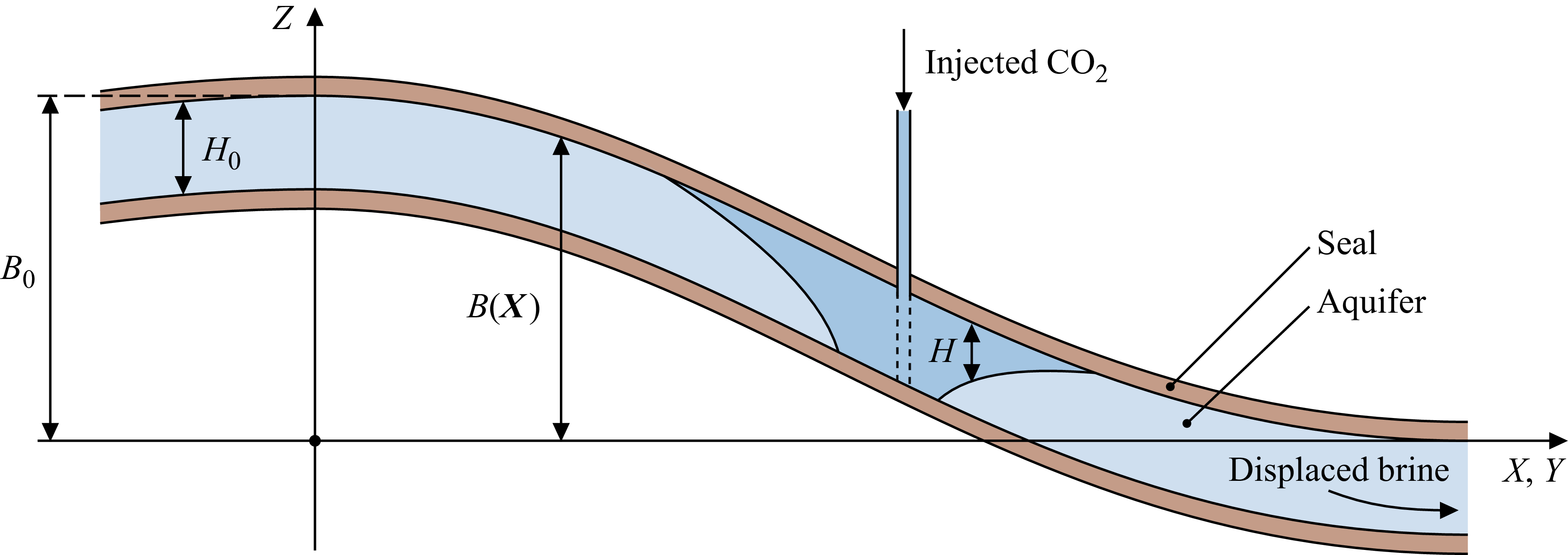
 CO2
CO2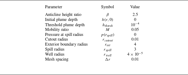
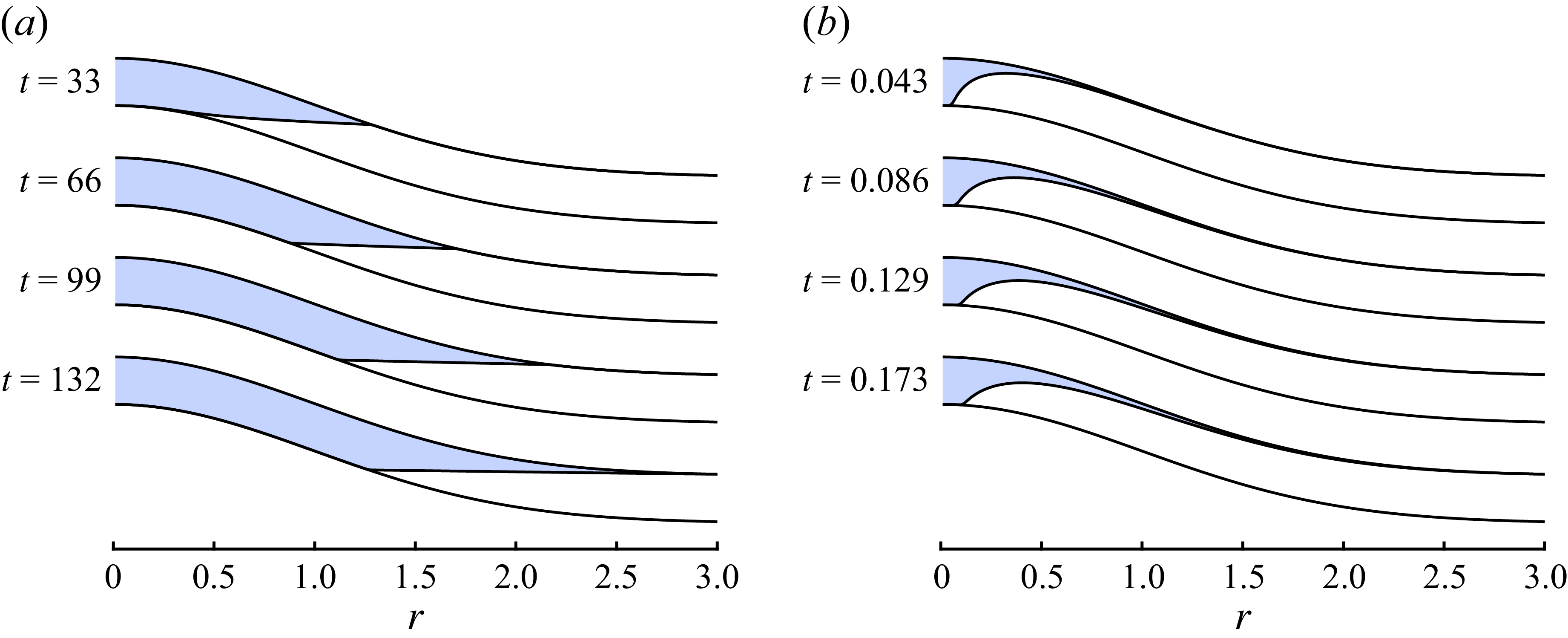
 CO2
CO2 v˙in=0.0785
 Λ=0.1
Λ=0.1 v˙in=7.85
 Λ=10
Λ=10
 v˙in=0.0785
 Λ=0.1
Λ=0.1 v˙in=7.85
 Λ=10
Λ=10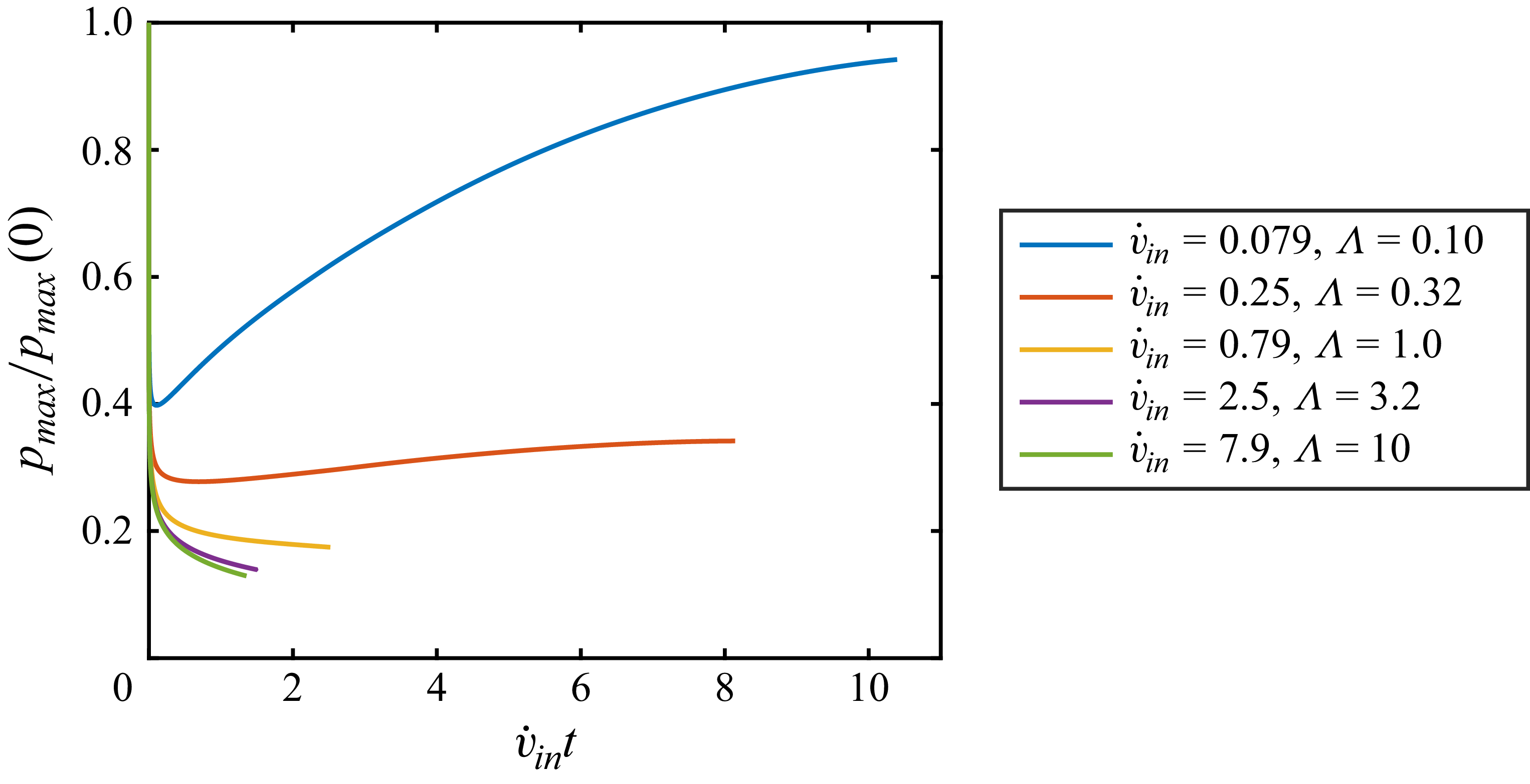
 CO2
CO2 pmax(0)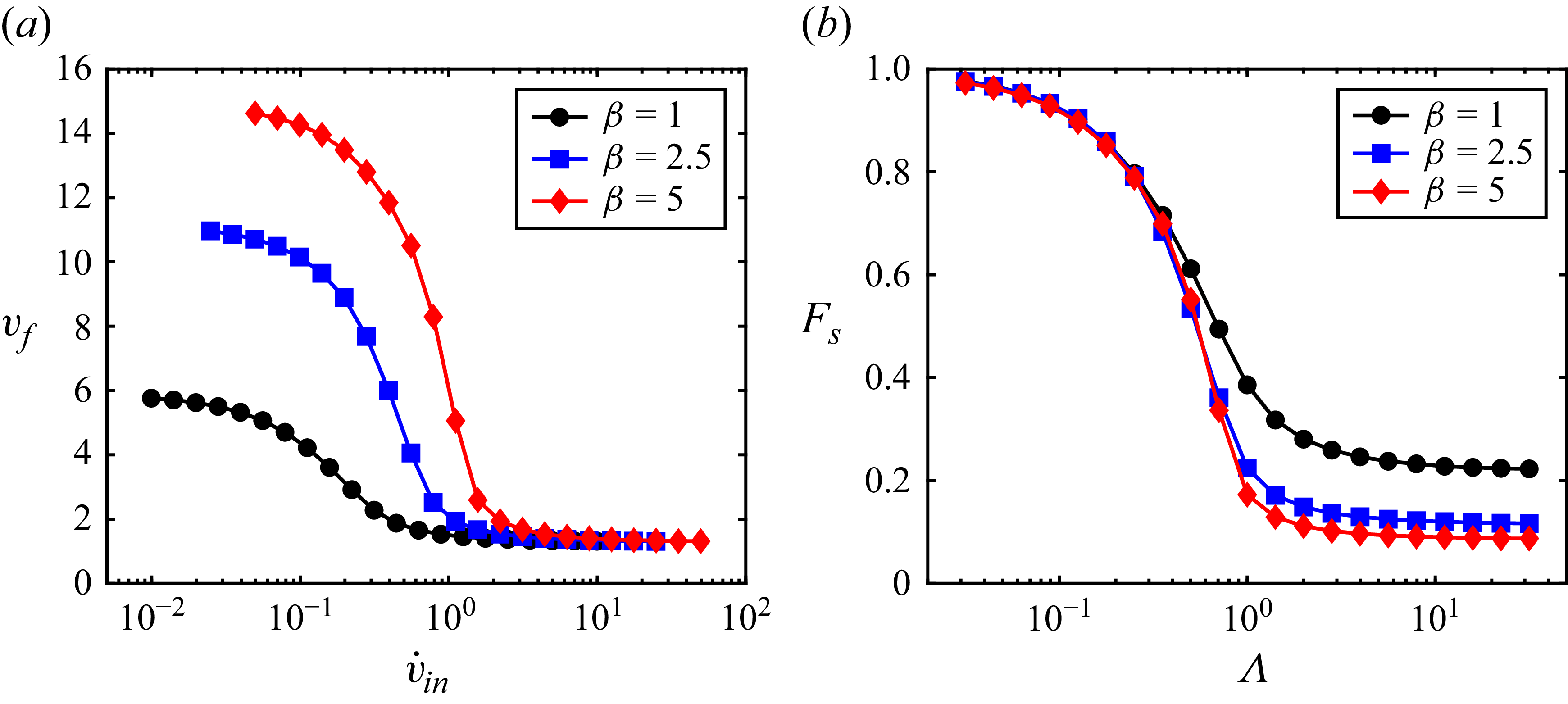
 CO2
CO2 vf
vf CO2
CO2 v˙in
v˙in β
β CO2
CO2 Fs
Fs CO2
CO2 Λ
Λ β
β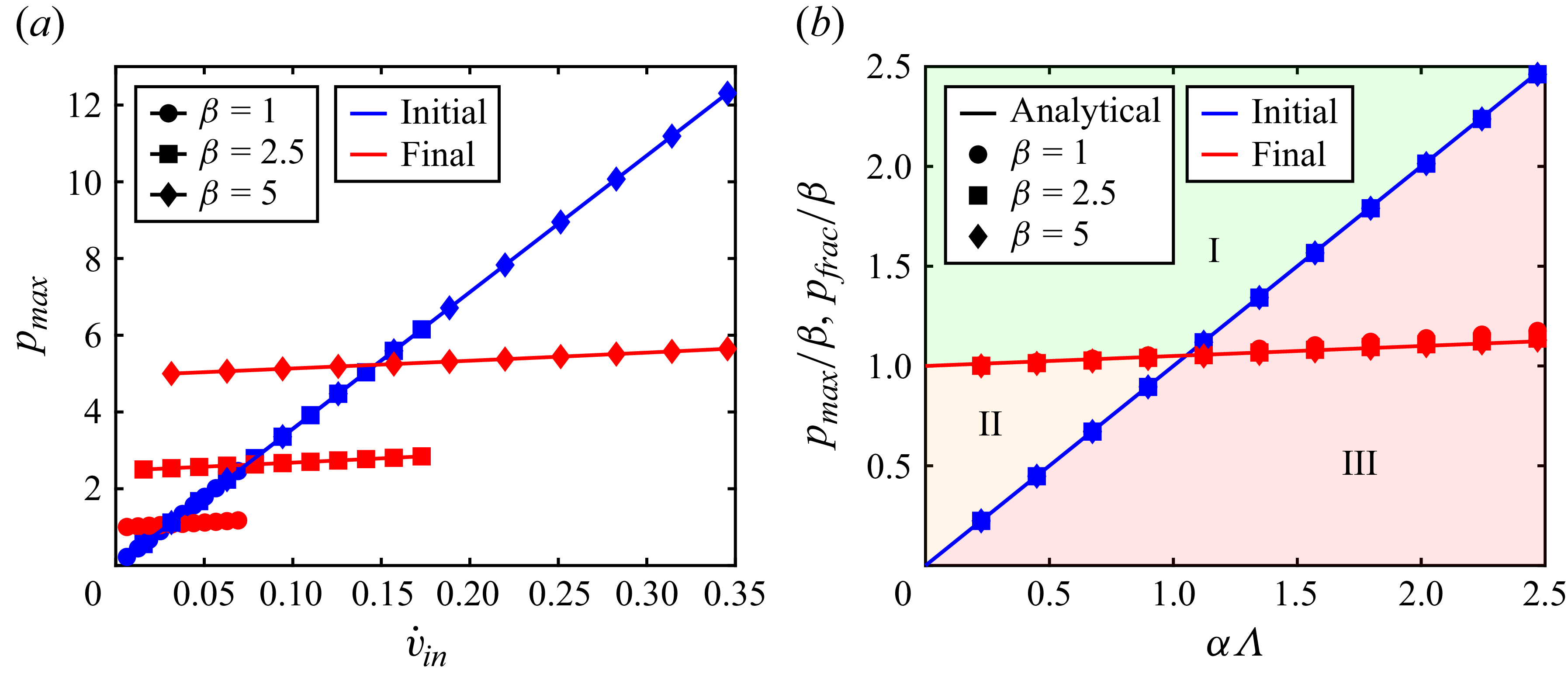
 CO2
CO2 v˙in
v˙in β
β β
β CO2
CO2 αN=1Λ
αN=1Λ CO2
CO2 pfrac
pfrac pfrac
pfrac pfrac
pfrac pfrac
pfrac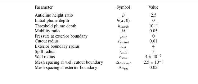
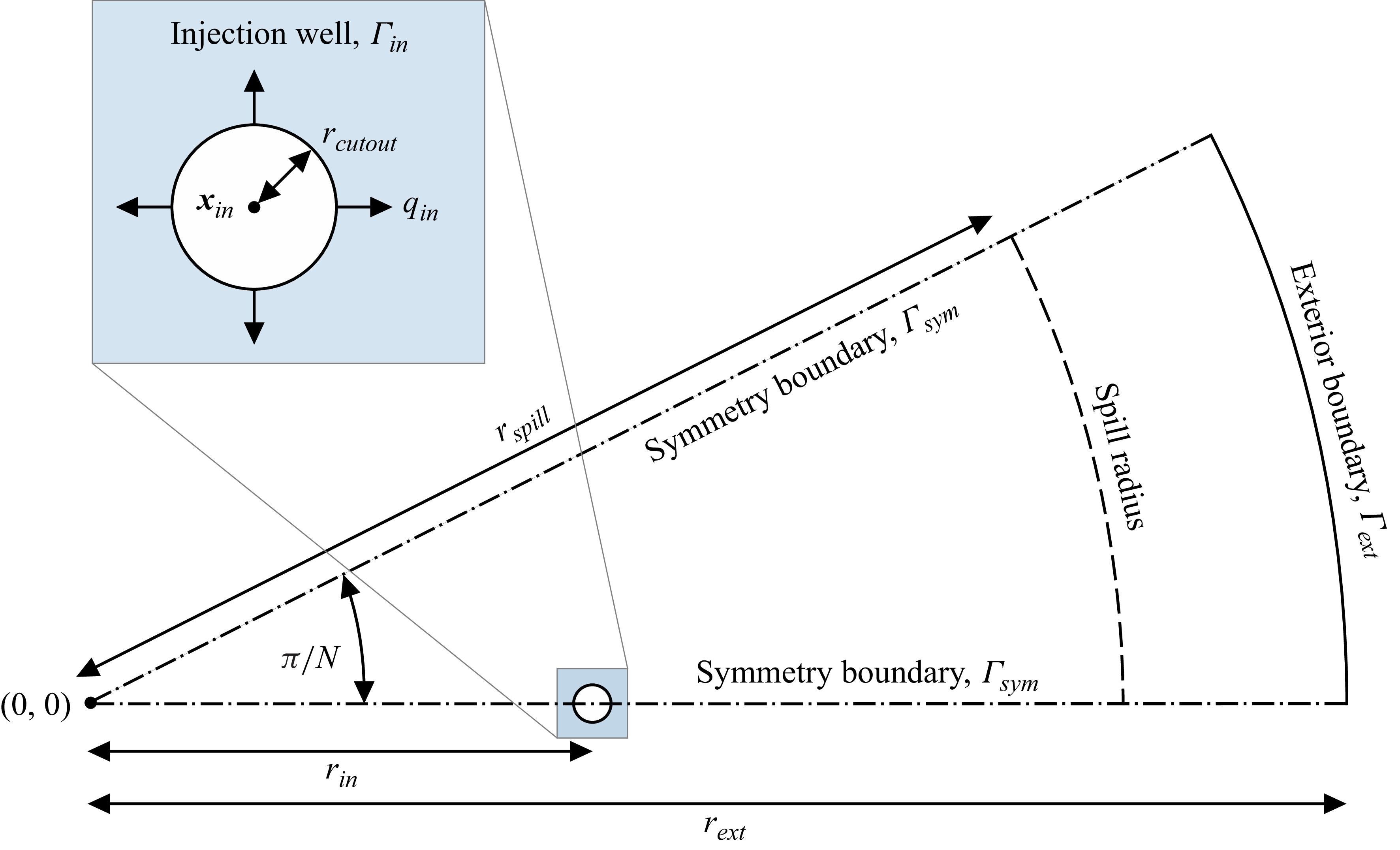
 N
N
 CO2
CO2 v˙in=0.0131
 Λ=0.1
Λ=0.1 rin=1
rin=1 t=34
t=34 t=69
t=69 t=103
t=103 t=138
t=138 h∈{0.1,0.2,…,1}
 h=hthresh
 CO2
CO2
 CO2
CO2 v˙in=1.31
 Λ=10
Λ=10 rin=1
rin=1 t=0.051
 t=0.102
 t=0.152
 t=0.203
 h∈{0.1,0.2,…,1}
 h=hthresh
 CO2
CO2
 v˙in=0.0131
 Λ=0.1
Λ=0.1 v˙in=1.31
 Λ=10
Λ=10 rin=1
rin=1 θ=0
θ=0 θ=π/6
θ=π/6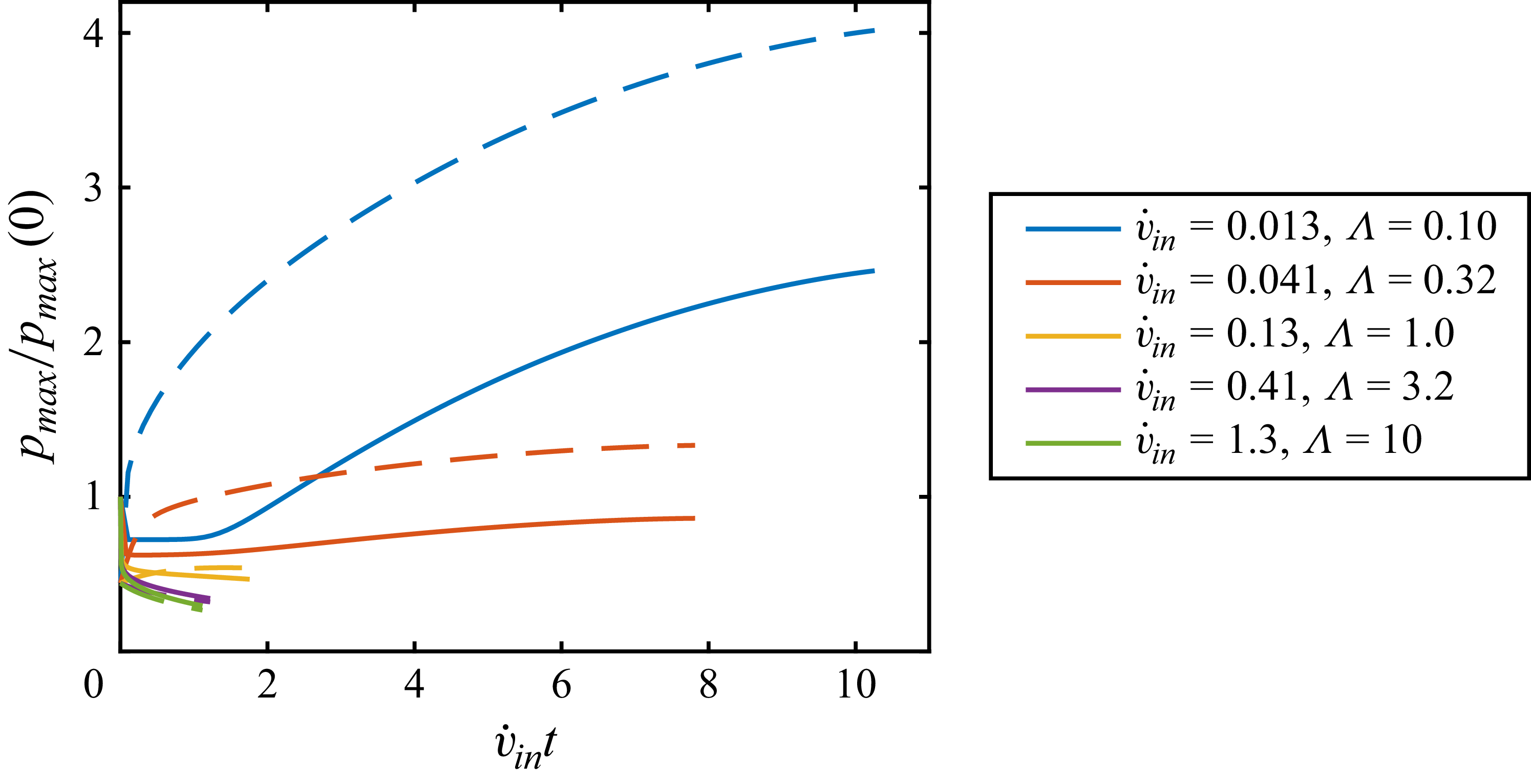
 CO2
CO2 rin=1
rin=1 pmax(0)
 CO2
CO2 Fs
Fs CO2
CO2 Λ
Λ N
N tf
tf h∈{hthresh,0.1,0.2,…,1}
 CO2
CO2 Fs
Fs CO2
CO2 Λ
Λ rin
rin tf
tf h∈{hthresh,0.1,0.2,…,1}
 β
β CO2
CO2 αΛ
αΛ CO2
CO2 pfrac
pfrac pfrac
pfrac pfrac
pfrac pfrac
pfrac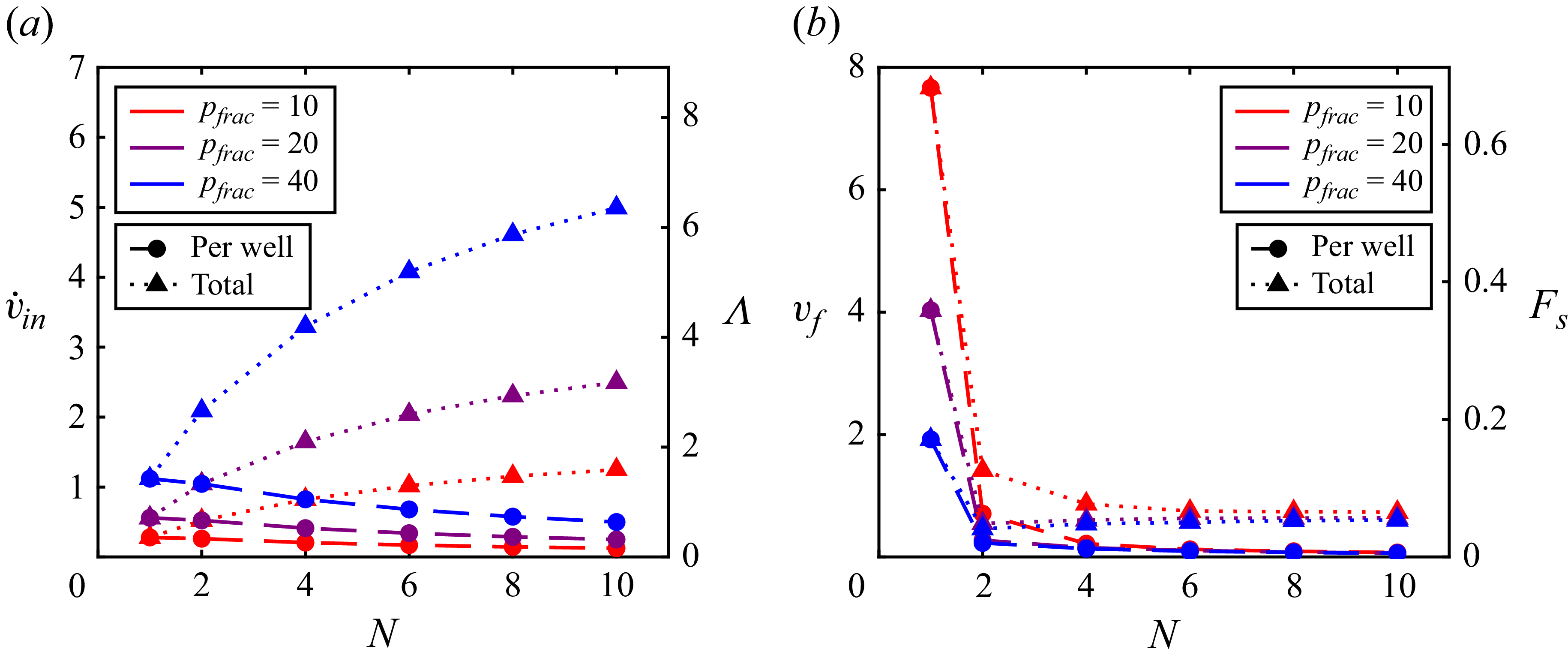
 CO2
CO2 pmax=pfrac
 N
N rin=1
rin=1 y
y Λ
Λ CO2
CO2 N
N rin=1
rin=1 y
y Fs
Fs N=1
N=1 N>1
N>1 N
N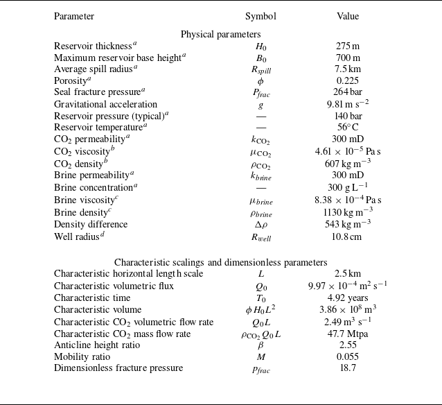
 CO2
CO2
 Open access

