


1. Introduction
Evaporation of colloidal suspension with induced particle deposition (figure 1 a) is ubiquitously observed in nature and widely applied in various engineering applications (Lauga & Brenner Reference Lauga and Brenner2004; Bhardwaj, Fang & Attinger Reference Bhardwaj, Fang and Attinger2009; Sáenz et al. Reference Sáenz, Wray, Che, Matar, Valluri, Kim and Sefiane2017; Brutin & Starov Reference Brutin and Starov2018; Wang et al. Reference Wang, Orejon, Takata and Sefiane2022b ; Wilson & D’Ambrosio Reference Wilson and D’Ambrosio2023), ranging from water purification (Wu et al. Reference Wu, Chen, Wang, Chen, Yang and Darling2021; Chiavazzo Reference Chiavazzo2022; Zhang et al. Reference Zhang, Li, Zhong, Leroy, Xu, Zhao and Wang2022; Song et al. Reference Song, Fang, Xu and Zhu2025), salt precipitation (He, Jiang & Xu Reference He, Jiang and Xu2019; Yang et al. Reference Yang, Pan, Dang, Gan and Han2022, Reference Yang, Lei, Wang, Xu, Chen and Luo2023, Reference Yang, Xu, Lei, Wang, Chen and Luo2025) and inkjet printing (Park & Moon Reference Park and Moon2006; Talbot et al. Reference Talbot, Yang, Berson and Bain2014; Masuda & Shimoda Reference Masuda and Shimoda2017; Lohse Reference Lohse2021) to self-assembly of particles (Boles, Engel & Talapin Reference Boles, Engel and Talapin2016; Gu et al. Reference Gu, Huang, Li, Li and Song2018; Qin et al. Reference Qin, Mazloomi Moqaddam, Del Carro, Kang, Brunschwiler, Derome and Carmeliet2019; Su et al. Reference Su2020; Li et al. Reference Li2021), and so on. The best-known example is the coffee ring formation (figure 1 b), where most of particles are swept to the pinned contact line of the droplet. Multi-ring patterns (figure 1 e,f) are reported when multiple stick-slip behaviour occurs, caused by sufficient contact angle hysteresis (Shmuylovich, Shen & Stone Reference Shmuylovich, Shen and Stone2002; Maheshwari et al. Reference Maheshwari, Zhang, Zhu and Chang2008; Moffat, Sefiane & Shanahan Reference Moffat, Sefiane and Shanahan2009; Yang, Li & Sun Reference Yang, Li and Sun2014). The `stick-slip’ motion is also termed `stick-slide’ in the literature, while the `multiple stick-slip’ process is also termed `stick-jump’ (Wilson & D’Ambrosio Reference Wilson and D’Ambrosio2023). Opposite to ring deposition patterns, a mountain-like deposition pattern (figure 1 d) is observed when a droplet evaporates with a receding contact line (Willmer et al. Reference Willmer, Baldwin, Kwartnik and Fairhurst2010; Li, Sheng & Tsao Reference Li, Sheng and Tsao2014). Uniform deposition patterns (figure 1 c) can be achieved by using non-spherical particles (Yunker et al. Reference Yunker, Still, Lohr and Yodh2011) or adjusting the pH value of the liquid (Bhardwaj et al. Reference Bhardwaj, Fang, Somasundaran and Attinger2010). Other deposition patterns, such as volcano-like and hexagonal cell type, have also been reported during evaporation of a polymer solution (Kajiya et al. Reference Kajiya, Monteux, Narita, Lequeux and Doi2009) or surfactant-laden aqueous droplet (Truskett & Stebe Reference Truskett and Stebe2003).
Illustration of various particle deposition patterns after evaporation of a colloidal droplet. (a) Colloidal droplet evaporation on a flat surface. (b) Coffee ring (Yunker et al. Reference Yunker, Still, Lohr and Yodh2011). (c) Uniform deposition pattern (Yunker et al. Reference Yunker, Still, Lohr and Yodh2011). (d) Mountain type (Li et al. Reference Li, Sheng and Tsao2014). (e) Symmetrical multiple rings (Yang et al. Reference Yang, Li and Sun2014). ( f) Unsymmetrical multiple rings (Maheshwari et al. Reference Maheshwari, Zhang, Zhu and Chang2008).

Droplet evaporation induced particle deposition is a complex multiple physical process, including liquid internal/interfacial flow, vapour transport, contact line motion, phase change with heat transfer, and particle transport/accumulation/deposition. The advanced modelling of such complex system, as well as the revealing of the coupled mechanisms, has long been a big challenge. Deegan et al. (Reference Deegan, Bakajin, Dupont, Huber, Nagel and Witten1997) first developed a theoretical model to explain the coffee ring mechanism, i.e. an internal capillary flow induced by different evaporation rates over the droplet surface drives the particles from the apex to the periphery of the droplet. Deegan et al. (Reference Deegan, Bakajin, Dupont, Huber, Nagel and Witten2000) also applied the theoretical model to predict liquid flow and particle distribution in evaporating droplets. In their work, particle convection is much more dominant than diffusion, i.e. they assume that the Péclet number ( $\textit{Pe}$
) is large. Petsi, Kalarakis & Burganos (Reference Petsi, Kalarakis and Burganos2010) studied deposition of Brownian particles during evaporation of two-dimensional (2-D) sessile droplets. They computed the trajectories of suspended Brownian particles during evaporation by using analytical expressions of the flow field, with the consideration of interaction between particles and evaporating free surface. The anisotropic diffusion due to solid substrate is also considered. They found that for a pinned contact line, large Péclet number leads to coffee ring deposition, while small Péclet number is beneficial for uniform and mountain-type depositions. For depinned contact lines, mountain-type depositions are generally formed. Frastia, Archer & Thiele (Reference Frastia, Archer and Thiele2011) proposed a dynamic model based on long-wave approximation to predict the regular and irregular multi-ring deposition patterns corresponding to stick-slip motions of the contact line. They also analysed how particle concentration and evaporation rate affect the deposition patterns. In their work, the particle diffusion coefficient depends on concentration and is calculated by the Einstein–Stokes relation.
$\textit{Pe}$
) is large. Petsi, Kalarakis & Burganos (Reference Petsi, Kalarakis and Burganos2010) studied deposition of Brownian particles during evaporation of two-dimensional (2-D) sessile droplets. They computed the trajectories of suspended Brownian particles during evaporation by using analytical expressions of the flow field, with the consideration of interaction between particles and evaporating free surface. The anisotropic diffusion due to solid substrate is also considered. They found that for a pinned contact line, large Péclet number leads to coffee ring deposition, while small Péclet number is beneficial for uniform and mountain-type depositions. For depinned contact lines, mountain-type depositions are generally formed. Frastia, Archer & Thiele (Reference Frastia, Archer and Thiele2011) proposed a dynamic model based on long-wave approximation to predict the regular and irregular multi-ring deposition patterns corresponding to stick-slip motions of the contact line. They also analysed how particle concentration and evaporation rate affect the deposition patterns. In their work, the particle diffusion coefficient depends on concentration and is calculated by the Einstein–Stokes relation.
Later, Kaplan & Mahadevan (Reference Kaplan and Mahadevan2015) developed a multiphase model by coupling the inhomogeneous evaporation rate, droplet internal flow and local particle concentration. They proposed a dimensionless number called the inverse capillary number, $\alpha = {\varepsilon ^4}/\textit{Ca}$
, to characterise the transition from ring to uniform deposition pattern, where
$\alpha = {\varepsilon ^4}/\textit{Ca}$
, to characterise the transition from ring to uniform deposition pattern, where $\varepsilon$
and
$\varepsilon$
and $\textit{Ca}$
are droplet aspect ratio and capillary number. Note that their capillary number is defined using the evaporation rate
$\textit{Ca}$
are droplet aspect ratio and capillary number. Note that their capillary number is defined using the evaporation rate $E_0$
instead of capillary convection velocity
$E_0$
instead of capillary convection velocity $u_c$
, i.e.
$u_c$
, i.e. $\textit{Ca} = {\mu _l}{E_0}/\sigma$
. Their results show that higher
$\textit{Ca} = {\mu _l}{E_0}/\sigma$
. Their results show that higher $\alpha \gg 1$
(capillary convection more dominant than droplet evaporation) leads to ring or band deposition patterns, while
$\alpha \gg 1$
(capillary convection more dominant than droplet evaporation) leads to ring or band deposition patterns, while $\alpha \ll 1$
results in uniform deposition patterns. In their work, particle convection is dominant over diffusion by assuming a very high Péclet number. Based on the modelling of fluid flow and contact line motion, Man & Doi (Reference Man and Doi2016) proposed a theory to predict deposition pattern change continuously from a ring to volcano-like to mountain-like transition. They found that the various deposition patterns depend on the mobility of the contact line and the evaporation rate. By assuming a standard model for the stick-slip motion of the contact line, Wu et al. (Reference Wu, Man and Doi2018) extended the theoretical model to realise the multi-ring pattern. In these works, particle convection is assumed more dominant than diffusion. Recently, D’Ambrosio et al. (Reference D’Ambrosio, Wilson, Wray and Duffy2023) proposed a mathematical model to consider the effect of droplet spatial evaporation flux on the deposition patterns. They introduced a free parameter
$\alpha \ll 1$
results in uniform deposition patterns. In their work, particle convection is dominant over diffusion by assuming a very high Péclet number. Based on the modelling of fluid flow and contact line motion, Man & Doi (Reference Man and Doi2016) proposed a theory to predict deposition pattern change continuously from a ring to volcano-like to mountain-like transition. They found that the various deposition patterns depend on the mobility of the contact line and the evaporation rate. By assuming a standard model for the stick-slip motion of the contact line, Wu et al. (Reference Wu, Man and Doi2018) extended the theoretical model to realise the multi-ring pattern. In these works, particle convection is assumed more dominant than diffusion. Recently, D’Ambrosio et al. (Reference D’Ambrosio, Wilson, Wray and Duffy2023) proposed a mathematical model to consider the effect of droplet spatial evaporation flux on the deposition patterns. They introduced a free parameter $n$
to analogise various evaporation conditions, and found that the range
$n$
to analogise various evaporation conditions, and found that the range $-1\lt n\lt 1$
leads to a ring deposition pattern, while
$-1\lt n\lt 1$
leads to a ring deposition pattern, while $n\gt 1$
leads to a mountain-like deposition pattern. In this model, they consider small reduced Péclet number, which corresponds to a large (but not too large) Péclet number. The free surface capture behaviour is in the limit of very large Péclet number. They also showed that at the condition of high
$n\gt 1$
leads to a mountain-like deposition pattern. In this model, they consider small reduced Péclet number, which corresponds to a large (but not too large) Péclet number. The free surface capture behaviour is in the limit of very large Péclet number. They also showed that at the condition of high $\textit{Pe}$
, all the particles are captured by the descending free surface before eventually being deposited onto the substrate. Moore, Vella & Oliver (Reference Moore, Vella and Oliver2021) presented a systematic asymptotic analysis of the solute profile as an axisymmetric droplet with a pinned contact line evaporates in the limit of large
$\textit{Pe}$
, all the particles are captured by the descending free surface before eventually being deposited onto the substrate. Moore, Vella & Oliver (Reference Moore, Vella and Oliver2021) presented a systematic asymptotic analysis of the solute profile as an axisymmetric droplet with a pinned contact line evaporates in the limit of large $\textit{Pe}$
. They found that the effect of solute diffusion close to the contact line can drive the formation of a nascent coffee ring at dilute stages of the evaporation process. Later, they extended this study to arbitrary droplet contact sets (Moore, Vella & Oliver Reference Moore, Vella and Oliver2022).
$\textit{Pe}$
. They found that the effect of solute diffusion close to the contact line can drive the formation of a nascent coffee ring at dilute stages of the evaporation process. Later, they extended this study to arbitrary droplet contact sets (Moore, Vella & Oliver Reference Moore, Vella and Oliver2022).
Regarding evaporation of non-spherical droplets, Sáenz et al. (Reference Sáenz, Wray, Che, Matar, Valluri, Kim and Sefiane2017) deduced a universal scaling law for the evaporation rate that is valid for any shape, and demonstrated that more curved regions lead to preferential localised deposition in particle-laden drops. Both particle advection and diffusion are considered in their theoretical model. Wray & Moore (Reference Wray and Moore2023) solved the evaporating flux of non-circular droplets using a novel asymptotic expansion approach, which is successfully applied to droplets with a wide range of footprint shapes. For non-isothermal evaporation, Dunn et al. (Reference Dunn, Wilson, Duffy, David and Sefiane2009) proposed a mathematical model that includes the variation of the saturation concentration with temperature, which coupled the vapour concentration in the atmosphere and the temperature in the liquid and the substrate. This model captured well the behaviour of the strong influence of substrate thermal conductivity on the evaporation of a pinned droplet. More developments on the theoretical modelling of evaporating sessile droplet and resulted deposition patterns are discussed in Wilson & D’Ambrosio (Reference Wilson and D’Ambrosio2023).
In terms of numerical modelling, Hu & Larson (Reference Hu and Larson2002) applied the finite element method (FEM) to analyse the droplet evaporation and compare with the analytical solution, and they derived an approximation of the evaporation rate. Hu & Larson (Reference Hu and Larson2005b
) further applied the FEM to simultaneously solve the liquid internal flow and vapour diffusion of an evaporating droplet, confirming the accuracy of lubrication theory at small droplet aspect ratio. By extending the lubrication theory and the FEM with Laplace’s equation to solve the temperature field, Hu & Larson (Reference Hu and Larson2005a
) studied the effects of Marangoni stress on the microflow in the evaporating droplet. Bhardwaj et al. (Reference Bhardwaj, Fang and Attinger2009) further developed the FEM to solve the coupled liquid flow, vapour diffusion and heat/mass transfer. By applying a continuum advection–diffusion equation to track the particle concentration, the modelled particle deposit shapes and sizes agree reasonably well with the experimental results. Widjaja & Harris (Reference Widjaja and Harris2008) numerically applied the Galerkin method/FEM to solve the particle deposition profiles on a solid substrate during evaporation of a colloidal droplet. They obtained the ring-shaped and uniform deposition patterns, and found that the deposition profile is influenced by the mass transfer of particles in the liquid bulk, and the deposition rate along the substrate. The competition between capillary convection and particle diffusion is investigated with different $\textit{Pe}$
. With the increase of
$\textit{Pe}$
. With the increase of $\textit{Pe}$
, ring-shaped deposition patterns are prone to be formed rather than uniform deposition patterns.
$\textit{Pe}$
, ring-shaped deposition patterns are prone to be formed rather than uniform deposition patterns.
Li et al. (Reference Li, Diddens, Segers, Wijshoff, Versluis and Lohse2020) investigated droplet evaporation on oil-wetted hydrophilic surfaces. They demonstrated both experimentally and numerically that the contact line dynamics can be tuned through the addition of a surfactant to control surface energies, which leads to control over the final particle deposition. Raju et al. (Reference Raju, Diddens, Li, Marin, van der Linden, Zhang and Lohse2022) investigated evaporation of a sessile colloidal water–glycerol droplet, and they found the formation of a Marangoni ring at a particular radial position near the liquid–air interface. By numerical simulations of multi-fields, Schofield et al. (Reference Schofield, Pritchard, Wilson and Sefiane2021) modelled the non-isothermal evaporation, and found that droplets on less conductive substrates have longer lifetimes than those on more conductive substrates. Erdem, Denner & Biancofiore (Reference Erdem, Denner and Biancofiore2024) proposed a numerical algorithm to study the influence of both pinned and moving contact line schemes on the droplet evaporation and particle deposition. They also investigated how the non-dimensional numbers such as Marangoni number, evaporation number, Damköhler number and Péclet number affect the deposition patterns. Crivoi & Duan (Reference Crivoi and Duan2013) studied the addition of surfactant inside a water suspension to promote or attenuate the coffee ring effect. By Monte Carlo simulations, they revealed that particle sticking probability is a crucial factor in the morphology of finally dried structures. Siregar, Kuerten & van der Geld (Reference Siregar, Kuerten and van der Geld2013) have developed a numerical model for simulating the evaporation of inkjet-printed droplets based on the method of lines. The model shows fair agreement with experiments for large droplet, but is not able to simulate the evaporation process for much smaller droplets. Chalmers, Smith & Archer (Reference Chalmers, Smith and Archer2017) developed a lattice gas model for the evaporation of droplets of a particle suspension. This model assumes diffusive dynamics but does not include the advective hydrodynamics of the solvent. With this model, they observed an equivalent of the coffee ring stain effect due to thermodynamics.
The above literature review illustrates the impressive performances of theoretical and numerical modelling in understanding evaporation of colloidal droplet and resultant particle deposition. Despite the great success, some mechanisms are not yet fully discovered, e.g. particle–particle interactions, particle–substrate interactions, the heterogeneity of the substrate, and the competition between capillary flow/particle diffusion under conjugate heat transfer. As an advanced numerical approach, the lattice Boltzmann model (LBM) (Higuera & Succi Reference Higuera and Succi1989, Reference Succi2018; Diotallevi et al. Reference Diotallevi, Biferale, Chibbaro, Lamura, Pontrelli, Sbragaglia, Succi and Toschi2009; Chen et al. Reference Chen, Kang, Mu, He and Tao2014; Li et al. Reference Li, Luo, Kang, He, Chen and Liu2016; Huang, Wu & Adams Reference Huang, Wu and Adams2021; Liu et al. Reference Liu, Lu, Li, Yu and Sahu2021) is advantageous in modelling multi-phase flows and phase change phenomena, since it can automatically capture the interface by incorporating intermolecular-level interactions. The LBMs to model evaporation of colloidal suspension and resulted particle deposition generally fall into two categories, i.e. the Lagrangian method and the Eulerian method. In the Lagrangian method, each particle is explicitly tracked, given that the force and torque for each particle as well as the particle–particle and particle–wall interactions are calculated. Joshi & Sun (Reference Joshi and Sun2009, Reference Joshi and Sun2010) first proposed 2-D and three-dimensional (3-D) LBMs in the Lagrangian framework to investigate the influence of particle volume fraction and size during colloidal droplet evaporation, and found that the final particle deposition can be controlled by substrate patterning and by the evaporation rate. Afterwards, Zhao & Yong (Reference Zhao and Yong2017) modelled the assembly and deposition of the surface-active particles in a evaporation sessile droplet with pinned contact line, and found that the particles migrate first towards the apex and then to the contact line as the droplet dries out. Recently, Wang & Cheng (Reference Wang and Cheng2021) combined a 2-D immersed boundary LBM with a non-isothermal liquid–vapour phase change model to simulate the evaporation-induced particle deposition. They found that at low contact angle with pinned contact line, a coffee ring pattern is obtained. On the other hand, at high contact angle with moving contact line, the Marangoni stress dominates, leading to a mountain-type deposition pattern. With a similar approach, Zhang et al. (Reference Zhang, Zhang, Zhao and Yang2021) found that a slippery contact line is not beneficial for a ring deposition pattern, but more likely leads to uniform or coffee eye deposition patterns, while the latter indicates deposition with a combination of the thick central stain and the thin outer ring (Li et al. Reference Li, Lv, Li, Quéré and Zheng2015).
Despite the successes of revealing some evaporation and deposition mechanisms, the Lagrangian methods share the drawbacks in modelling realistic, massive particles as well as high-performance parallelisation. These drawbacks can be easily overcome using the Eulerian method, since the number of particles is simply represented as solute concentration. For example, Qin et al. (Reference Qin, Mazloomi Moqaddam, Del Carro, Kang, Brunschwiler, Derome and Carmeliet2019, Reference Qin, Su, Zhao, Mazloomi Moqaddam, Carro, Brunschwiler, Kang, Song, Derome and Carmeliet2020) combined the two-phase LBM with temperature and solute transport to model evaporation of colloidal suspension in various micropore structures. This model was further extended to consider the effects of particle accumulation on local fluid viscosity, surface tension and evaporation rate (Qin et al. Reference Qin, Fei, Zhao, Kang, Derome and Carmeliet2023). Nath & Ray (Reference Nath and Ray2021) numerically manipulated the surface chemical heterogeneity to control contact line motion, to realise desirable deposited microstructure after evaporation of a particle-laden droplet. Yang et al. (Reference Yang, Lei, Wang, Xu, Chen and Luo2023) combined the two-phase LBM with a phase change model and salt growth model to realise the brine evaporation and resultant salt precipitation. The drawback of the Eulerian-type model lies in that by using concentration to represent the particles, it neglects the influence of particle size and shape. Compared with the Lagrangian-type method, which directly resolves each single particle, it is incapable of modelling the particle–particle (Joshi & Sun Reference Joshi and Sun2010), particle–interface (Yunker et al. Reference Yunker, Still, Lohr and Yodh2011) and particle–substrate (Xie & Harting Reference Xie and Harting2018) interactions. As a matter of fact, the Eulerian-type model is advantageous in modelling overall accumulation behaviour with a large number of particles, which does not concern the local interactions. However, for the detailed study of the above-mentioned particle interaction with particle, interface and substrate, and so on, the Lagrangian method introduced above is advantageous and irreplaceable. It is noteworthy that the LBM is a mesoscopic model situated between microscale and macroscale. To compare it with macroscopic results, the unit conversion from lattice unit to physical unit has to be conducted (Liu, Zhang & Valocchi Reference Liu, Zhang and Valocchi2015; Wang et al. Reference Wang, Tong, He and Liu2022a ).
From the above introduction, we can clearly observe that despite the extensive efforts of previous studies of LBM developments, the realisation of diverse experimentally observed deposition patterns, and a comprehensive analysis/characterisation of the effects of various surface/liquid/particle properties on the evaporation dynamics, as well as deposition patterns, are still lacking. In this work, we tackle exactly this challenging task. In the following, we first introduce the double-distribution multiple-relaxation-time (MRT) LBM with the contact angle hysteresis model in § 2, for the modelling of isothermal two-phase flow, phase change and particle transport and deposition. Afterwards, in § 3, the model is validated by droplet evaporation and coffee ring deposition pattern, with the comparison of theoretical/experimental results. In § 4, the model is applied to reproduce the ring to uniform to mountain-type deposition patterns, experiencing single or multiple symmetrical/unsymmetrical stick-slip processes, under the conditions of uniform/non-uniform surface wettability hysteresis. Then combining with the particle transport equation, we unveil a scaling relation linking the characteristic features of the deposition pattern to a single dimensionless parameter. To the best of our knowledge, this is the first time that the diverse deposition patterns are reproduced and well characterised by LBMs. Finally, § 5 concludes the present work.
2. Numerical modelling
In this section, we introduce the Eulerian-type LBM of isothermal colloidal droplet evaporation and resultant particle deposition. We apply a double-distribution LBM, with one distribution function $f$
to model the liquid–vapour two-phase flow and evaporation, and another distribution function
$f$
to model the liquid–vapour two-phase flow and evaporation, and another distribution function $g$
to model the particle transport and deposition.
$g$
to model the particle transport and deposition.
2.1. The liquid–vapour two-phase model
2.1.1. The MRT pseudopotential LBM
To model the two-phase flow, we apply the improved MRT pseudopotential two-phase LBM (Li, Luo & Li Reference Li, Luo and Li2013), with the governing equation
 \begin{equation} {f_i}({\boldsymbol {x}} + {\boldsymbol {c}_{{i}}}\,\Delta t,t + \Delta t) = {f_i}(\boldsymbol {x},t) - {({\boldsymbol {M}^{ { - 1}}}\boldsymbol{{\varLambda M}})_\textit{ij}}({f_{\!j}} - f_{\!j}^{\textit{eq}}) + \delta t\,R_i, \end{equation}
where $f_i$
(
$f_i$
( $f_i^{\textit{eq}}$
) is the (equilibrium) discrete density distribution function,
$f_i^{\textit{eq}}$
) is the (equilibrium) discrete density distribution function, ${\boldsymbol {c}_{\boldsymbol {i}}} = ({c_{ix}},{c_{iy}})$
is the discrete velocity in the
${\boldsymbol {c}_{\boldsymbol {i}}} = ({c_{ix}},{c_{iy}})$
is the discrete velocity in the $i$
th direction,
$i$
th direction, $\delta t$
is the time step,
$\delta t$
is the time step, $R_i$
represents the forcing term in the velocity space,
$R_i$
represents the forcing term in the velocity space, $\boldsymbol{{\varLambda }} = (\tau _\rho ^{ - 1},\tau _{{e}}^{ - 1},\tau _\zeta ^{ - 1},\tau _j^{ - 1},\tau _q^{ - 1},\tau _j^{ - 1},\tau _q^{ - 1},\tau _v^{ - 1},\tau _v^{ - 1})$
is the diagonal matrix, and
$\boldsymbol{{\varLambda }} = (\tau _\rho ^{ - 1},\tau _{{e}}^{ - 1},\tau _\zeta ^{ - 1},\tau _j^{ - 1},\tau _q^{ - 1},\tau _j^{ - 1},\tau _q^{ - 1},\tau _v^{ - 1},\tau _v^{ - 1})$
is the diagonal matrix, and $\boldsymbol {M}$
is the orthogonal transformation matrix. In this work, we apply the D2Q9 LBM, where the 9 discrete velocities (see figure S1 in the supplementary material available at https://doi.org/10.1017/jfm.2025.11067.), the transformation matrix
$\boldsymbol {M}$
is the orthogonal transformation matrix. In this work, we apply the D2Q9 LBM, where the 9 discrete velocities (see figure S1 in the supplementary material available at https://doi.org/10.1017/jfm.2025.11067.), the transformation matrix $\boldsymbol{M}$
and its inverse
$\boldsymbol{M}$
and its inverse $\boldsymbol{M}^{-1}$
are given in the supplementary material. Using the transformation matrix, the right-hand side of (2.1) can be rewritten as
$\boldsymbol{M}^{-1}$
are given in the supplementary material. Using the transformation matrix, the right-hand side of (2.1) can be rewritten as
 \begin{equation} \boldsymbol {m}^* = \boldsymbol {m} - \boldsymbol{{\varLambda }}(\boldsymbol {m}-{\boldsymbol {m}^{\textit{eq}}}) + \delta t\left(\boldsymbol {I} - \frac {\boldsymbol{{\varLambda }}}{2}\right)\boldsymbol {S} + \delta t\,\boldsymbol {C}, \end{equation}
where $\boldsymbol {m} = \boldsymbol {{M\!f}}$
,
$\boldsymbol {m} = \boldsymbol {{M\!f}}$
, $\boldsymbol {I}$
is the unit tensor,
$\boldsymbol {I}$
is the unit tensor, $\boldsymbol {S}$
is the forcing term in the moment space with
$\boldsymbol {S}$
is the forcing term in the moment space with $(\boldsymbol {I} - ( {\boldsymbol{{\varLambda }}}/{2}))\boldsymbol {S} = \boldsymbol {{M\!F}}$
, and
$(\boldsymbol {I} - ( {\boldsymbol{{\varLambda }}}/{2}))\boldsymbol {S} = \boldsymbol {{M\!F}}$
, and $\delta t\,\boldsymbol {C}$
is the additional term to independently adjust the surface tension
$\delta t\,\boldsymbol {C}$
is the additional term to independently adjust the surface tension $\sigma _{lv}$
(Li & Luo Reference Li and Luo2013). The equilibria
$\sigma _{lv}$
(Li & Luo Reference Li and Luo2013). The equilibria $\boldsymbol {m}^{\textit{eq}}$
are given by (Li et al. Reference Li, Luo and Li2013)
$\boldsymbol {m}^{\textit{eq}}$
are given by (Li et al. Reference Li, Luo and Li2013)
 \begin{equation} {\boldsymbol {m}^{\textit{eq}}} = \rho {(1, - 2 + 3\,|\boldsymbol {u}{|^2},1 - 3\,|\boldsymbol {u}{|^2},{u_x}, - {u_x},{u_y}, - {u_y},u_x^2 - u_y^2,{u_x}{u_y})^{\textrm{T}}}. \end{equation}
In the diagonal matrix, the parameters are selected as $\tau _\rho ^{ - 1} = \tau _j^{ - 1} = 1.0,\ \tau _{{e}}^{ - 1} = \tau _\zeta ^{ - 1} = \tau _q^{ - 1} = 1.1$
to achieve good stability. The relaxation time
$\tau _\rho ^{ - 1} = \tau _j^{ - 1} = 1.0,\ \tau _{{e}}^{ - 1} = \tau _\zeta ^{ - 1} = \tau _q^{ - 1} = 1.1$
to achieve good stability. The relaxation time $\tau _v$
is determined using the fluid kinematic viscosity with
$\tau _v$
is determined using the fluid kinematic viscosity with $v = ({\tau _v} - 0.5)c_s^2$
, where
$v = ({\tau _v} - 0.5)c_s^2$
, where ${c_s} = 1/\sqrt 3$
is the speed of sound. The propagation process of the MRT LBM is
${c_s} = 1/\sqrt 3$
is the speed of sound. The propagation process of the MRT LBM is
 \begin{equation} {f_i}(\boldsymbol {x} + {\boldsymbol {c}_{{i}}}\Delta t,t + \Delta t) = f_i^*(\boldsymbol {x},t), \end{equation}
with the post-collision distribution $f^* = \boldsymbol{M}^{- 1}\boldsymbol{m}^*$
. The macroscopic forcing terms
$f^* = \boldsymbol{M}^{- 1}\boldsymbol{m}^*$
. The macroscopic forcing terms $\boldsymbol {S}$
from Li et al. (Reference Li, Luo and Li2013) are used:
$\boldsymbol {S}$
from Li et al. (Reference Li, Luo and Li2013) are used:
 \begin{equation} \boldsymbol {S} = \left [ {\begin{array}{*{20}{c}} 0\\ {6({u_x}{F_x} + {u_y}{F_y}) + 12\chi\, |\boldsymbol {F}{|^2}/[{\psi ^2}\,\delta t\,({\tau _e} - 0.5)]}\\ { - 6({u_x}{F_x} + {u_y}{F_y}) - 12\chi\, |\boldsymbol {F}{|^2}/[{\psi ^2}\,\delta t\,({\tau _\varsigma } - 0.5)]}\\ {{F_x}}\\ { - {F_x}}\\ {{F_y}}\\ { - {F_y}}\\ {2({u_x}{F_x} - {u_y}{F_y})}\\ {{u_x}{F_y} + {u_y}{F_x}} \end{array}} \right ]\!, \end{equation}
where $|\boldsymbol {F}| = \sqrt {F_x^2 + F_y^2}$
,
$|\boldsymbol {F}| = \sqrt {F_x^2 + F_y^2}$
, $\chi$
is a tuning parameter, set to 0.105 to achieve thermodynamic consistency (Li, Luo & Li Reference Li, Luo and Li2012; Qin et al. Reference Qin, Fei, Zhao, Kang, Derome and Carmeliet2023), and
$\chi$
is a tuning parameter, set to 0.105 to achieve thermodynamic consistency (Li, Luo & Li Reference Li, Luo and Li2012; Qin et al. Reference Qin, Fei, Zhao, Kang, Derome and Carmeliet2023), and $\psi$
is the interaction potential, which will be given later. Generally,
$\psi$
is the interaction potential, which will be given later. Generally, $\boldsymbol {F}$
includes fluid–fluid/fluid–solid interaction
$\boldsymbol {F}$
includes fluid–fluid/fluid–solid interaction $\boldsymbol {F}_f$
and other body forces, where
$\boldsymbol {F}_f$
and other body forces, where $\boldsymbol {F}_f$
is given by
$\boldsymbol {F}_f$
is given by
 \begin{equation} {\boldsymbol {F}_f} = - G\,\psi (\boldsymbol {x})\sum \limits _{i = 1}^8 {w(|{\boldsymbol {c}_i}{|^2})}\, \psi (\boldsymbol {x} + {\boldsymbol {c}_i})\,{\boldsymbol {c}_i}, \end{equation}
where $G = - 1$
is the interaction strength, and
$G = - 1$
is the interaction strength, and $w(|{\boldsymbol {c}_i}{|^2})$
are the weights. The interaction potential
$w(|{\boldsymbol {c}_i}{|^2})$
are the weights. The interaction potential $\psi$
is given by incorporating the non-ideal equation of state (EoS)
$\psi$
is given by incorporating the non-ideal equation of state (EoS) $p_{\textit{EoS}}$
as
$p_{\textit{EoS}}$
as $\psi = \sqrt {{{2({p_{\textit{EoS}}} - \rho c_s^2)} \mathord {\left /{\vphantom {{2({p_{\textit{EoS}}} - \rho c_s^2)} {G{c^2}}}} \right .} {G{c^2}}}}$
(Yuan & Schaefer Reference Yuan and Schaefer2006). In this paper, we use the Carnahan–Starling EoS:
$\psi = \sqrt {{{2({p_{\textit{EoS}}} - \rho c_s^2)} \mathord {\left /{\vphantom {{2({p_{\textit{EoS}}} - \rho c_s^2)} {G{c^2}}}} \right .} {G{c^2}}}}$
(Yuan & Schaefer Reference Yuan and Schaefer2006). In this paper, we use the Carnahan–Starling EoS:
 \begin{equation} {p_{\textit{EoS}}} = \rho RT\frac {{1 + b\rho /4 + {{(b\rho /4)}^2} - {{(b\rho /4)}^3}}}{{{{(1 - b\rho /4)}^3}}} - a{\rho ^2}, \end{equation}
where $a$
is the parameter that determines the attraction of fluid molecules,
$a$
is the parameter that determines the attraction of fluid molecules, $b$
is the parameter to consider the volume of the non-ideal fluid, and
$b$
is the parameter to consider the volume of the non-ideal fluid, and $R$
is the gas constant. The values of
$R$
is the gas constant. The values of $a$
and
$a$
and $b$
are determined by the critical parameters of the fluid, i.e.
$b$
are determined by the critical parameters of the fluid, i.e. $a = 0.4963{R^2}T_c^2/{p_c},\ b = 0.18727R{T_c}/{p_c}$
, where
$a = 0.4963{R^2}T_c^2/{p_c},\ b = 0.18727R{T_c}/{p_c}$
, where $T_c$
and
$T_c$
and $p_c$
are critical temperature and pressure, respectively. In the current simulations,
$p_c$
are critical temperature and pressure, respectively. In the current simulations, $a = 1,\ b = 4,\ R = 1$
are used following Yuan & Schaefer (Reference Yuan and Schaefer2006) to achieve good stability and relatively low spurious current around the liquid–vapour interface. To implement the contact angle and its hysteresis, we introduce the fluid–solid interaction
$a = 1,\ b = 4,\ R = 1$
are used following Yuan & Schaefer (Reference Yuan and Schaefer2006) to achieve good stability and relatively low spurious current around the liquid–vapour interface. To implement the contact angle and its hysteresis, we introduce the fluid–solid interaction $\boldsymbol {F}_s$
similar to (2.6), i.e.
$\boldsymbol {F}_s$
similar to (2.6), i.e. ${\boldsymbol {F}_s} = - G\,\psi (\boldsymbol {x})\sum_{i = 1}^8 {w(|{\boldsymbol {c}_i}{|^2})}\, I(\boldsymbol {x} + {\boldsymbol {c}_i})\,\psi (\boldsymbol {x} + {\boldsymbol {c}_i})\,{\boldsymbol {c}_i}$
, where
${\boldsymbol {F}_s} = - G\,\psi (\boldsymbol {x})\sum_{i = 1}^8 {w(|{\boldsymbol {c}_i}{|^2})}\, I(\boldsymbol {x} + {\boldsymbol {c}_i})\,\psi (\boldsymbol {x} + {\boldsymbol {c}_i})\,{\boldsymbol {c}_i}$
, where $I(\boldsymbol {x} + {\boldsymbol {c}_i})$
is an indicator function equalling 1 at a solid node, and 0 at a fluid node. The calculation of
$I(\boldsymbol {x} + {\boldsymbol {c}_i})$
is an indicator function equalling 1 at a solid node, and 0 at a fluid node. The calculation of $\psi (\boldsymbol {x} + {\boldsymbol {c}_i})$
at a wall node uses the virtual wall density
$\psi (\boldsymbol {x} + {\boldsymbol {c}_i})$
at a wall node uses the virtual wall density $\rho _w$
by
$\rho _w$
by $\psi = \sqrt {2({p_{\textit{EoS}}}({\rho _w}) - {\rho _w}c_s^2)/G{c^2}}$
. The rule to determine
$\psi = \sqrt {2({p_{\textit{EoS}}}({\rho _w}) - {\rho _w}c_s^2)/G{c^2}}$
. The rule to determine $\rho _w$
will be discussed in § 2.1.2. The additional source term
$\rho _w$
will be discussed in § 2.1.2. The additional source term $\delta t\,\boldsymbol {C}$
at the right-hand side of (2.2) is given as (Li & Luo Reference Li and Luo2013)
$\delta t\,\boldsymbol {C}$
at the right-hand side of (2.2) is given as (Li & Luo Reference Li and Luo2013)
 \begin{equation} \boldsymbol {C} = \left [ {\begin{array}{*{20}{c}} 0\\ {1.5\tau _e^{ - 1}({Q_{\textit{xx}}} + {Q_{\textit{yy}}})}\\ { - 1.5\tau _\zeta ^{ - 1}({Q_{\textit{xx}}} + {Q_{\textit{yy}}})}\\ 0\\ 0\\ 0\\ 0\\ { - \tau _v^{ - 1}({Q_{\textit{xx}}} - {Q_{\textit{yy}}})}\\ { - \tau _v^{ - 1}{Q_{\textit{xy}}}} \end{array}} \right ]\!, \end{equation}
where the variables ${Q_{\textit{xx}}},{Q_{\textit{yy}}},{Q_{\textit{xy}}}$
are calculated using
${Q_{\textit{xx}}},{Q_{\textit{yy}}},{Q_{\textit{xy}}}$
are calculated using
 \begin{equation} \boldsymbol {Q} = \kappa \frac {G}{2}\,\psi (\boldsymbol {x})\sum \limits _{i = 1}^8 {w(|{\boldsymbol {c}_i}{|^2})}\, [\psi (\boldsymbol {x} + {\boldsymbol {c}_i}) - \psi (\boldsymbol {x})]\,{\boldsymbol {c}_i}{\boldsymbol {c}_i}, \end{equation}
and $\kappa \in (0,1)$
is a parameter to tune the surface tension. The resultant surface tension follows a simple linear decrease of
$\kappa \in (0,1)$
is a parameter to tune the surface tension. The resultant surface tension follows a simple linear decrease of $\kappa$
as
$\kappa$
as
 \begin{equation} {\sigma _{lv}}/{\sigma _{lv,0}} = 1 - \kappa , \end{equation}
where $\sigma _{lv,0}$
is the initial liquid–vapour surface tension with the tuning parameter
$\sigma _{lv,0}$
is the initial liquid–vapour surface tension with the tuning parameter $\kappa = 0$
. With the above equations, the Navier–Stokes equations can be recovered as
$\kappa = 0$
. With the above equations, the Navier–Stokes equations can be recovered as
 \begin{equation} \begin{array}{*{20}{c}} {\dfrac {{\partial \rho }}{{\partial t}} + \boldsymbol{\nabla }\boldsymbol{\cdot } (\rho \boldsymbol {u}) = 0},\\ {\dfrac {{\partial (\rho \boldsymbol {u})}}{{\partial t}} + \boldsymbol{\nabla }\boldsymbol{\cdot } (\rho \boldsymbol {uu}) = - \boldsymbol{\nabla }\boldsymbol{\cdot } \boldsymbol {P} + \boldsymbol{\nabla }\boldsymbol{\cdot } \left[\rho v(\boldsymbol{\nabla }\boldsymbol {u} + {{(\boldsymbol{\nabla }\boldsymbol {u})}^{\textrm{T}}})\right] + \boldsymbol {F}}, \end{array} \end{equation}
where the macroscopic variables of the two-phase flow are calculated as
 \begin{equation} \rho = \sum \limits _{i = 0}^8 {{f_i}} ,\quad \boldsymbol {u} = \frac {1}{\rho }\left(\sum \limits _{i = 0}^8 {{f_i}} {\boldsymbol {c}_i} + \frac {{\delta t\boldsymbol {F}}}{2}\right)\!. \end{equation}
As we explained in the Introduction, the above-obtained macroscopic variables are in lattice units. To make them comparable with physical results, the unit conversion has to be conducted. The most common approach is to convert the units with basic reference quantities, such as length, time and mass. Detailed unit conversion is given in § 3.2.
2.1.2. Implementation of contact angle and its hysteresis
To accurately prescribe the contact angle in a wide range with small spurious current, we apply the geometric formulation scheme (Ding & Spelt Reference Ding and Spelt2007) suitable for flat surfaces, where the contact angle $\theta$
(figure 2
a) satisfies the relation
$\theta$
(figure 2
a) satisfies the relation
 \begin{equation} \tan \left(\frac {\pi }{2} - \theta \right) = - \frac {{\partial \rho /\partial y}}{{\left | {\partial \rho /\partial x} \right |}}. \end{equation}
(a) Droplet on a flat surface with contact angle $\theta$
, where
$\theta$
, where $\boldsymbol {n}_s$
is the surface vector of the liquid–vapour interface pointing to the vapour phase. (b) Illustration of the halfway bounce-back scheme on a flat surface.
$\boldsymbol {n}_s$
is the surface vector of the liquid–vapour interface pointing to the vapour phase. (b) Illustration of the halfway bounce-back scheme on a flat surface.

In this paper, the halfway bounce-back scheme is applied to realise the no-slip boundary, as shown in figure 2(b). Under this condition, the partial derivatives in (2.13) are calculated by
 \begin{equation} \left \{ {\begin{array}{*{20}{c}} {\dfrac {{\partial {\rho _{x,1/2}}}}{{\partial x}} = 1.5\dfrac {{\partial {\rho _{x,1}}}}{{\partial x}} - 0.5\dfrac {{\partial {\rho _{x,2}}}}{{\partial x}},\quad \textrm{where}\quad \dfrac {{\partial {\rho _{x,y}}}}{{\partial x}} = \dfrac {{{\rho _{x + 1,y}} - {\rho _{x - 1,y}}}}{{2\,\delta x}},}\\ {\dfrac {{\partial {\rho _{x,1/2}}}}{{\partial y}} = \dfrac {{{\rho _{x,1}} - {\rho _{x,0}}}}{{\delta y}}. } \end{array}} \right . \end{equation}
Using standard lattices with $\delta x = \delta y = 1$
, and by combining (2.13) and (2.14), the wall density is expressed as
$\delta x = \delta y = 1$
, and by combining (2.13) and (2.14), the wall density is expressed as
 \begin{equation} {\rho _w} = {\rho _{x,0}} = {\rho _{x,1}} + \tan\! \left(\frac {\pi }{2} - \theta \right)\left | {\partial {\rho _{x,1/2}}/\partial x} \right |\!. \end{equation}
For the automatic measurement of local contact angle, we use the transformation of (2.13), i.e.
 \begin{equation} {\theta _m} = \frac {\pi }{2} + \textrm {atan}\left(\frac {{\partial \rho /\partial y}}{{\left | {\partial \rho /\partial x} \right |}}\right)\!. \end{equation}
The measured local contact angle is used to implement contact angle hysteresis. For simplicity, we use the contact angle hysteresis scheme proposed in Liu et al. (Reference Liu, Zhang and Valocchi2015) for colloidal droplet evaporation on a flat surface. Within the given contact angle hysteresis range $({\theta _R},{\theta _A})$
, the prescribed contact angle
$({\theta _R},{\theta _A})$
, the prescribed contact angle $\theta _p$
at next iteration should be
$\theta _p$
at next iteration should be
 \begin{equation} {} {}\left\{ {\begin{array}{*{20}{l}} {} {} {} {}{\theta _p}(t + \delta t) = {\theta _m}(t),\ {\theta _R} \lt {\theta _m}(t) \lt {\theta _A}\\ {} {} {} {}{\theta _p}(t + \delta t) = {\theta _R},\ {\theta _m}(t) \leqslant {\theta _R}\\ {} {} {} {}{\theta _p}(t + \delta t) = {\theta _A},\ {\theta _m}(t) \geqslant {\theta _A} {} {}\end{array}} \right.. {}\end{equation}
With this contact angle hysteresis scheme, when the measured contact angle ${\theta _m}$
increases to the advancing contact angle
${\theta _m}$
increases to the advancing contact angle ${\theta _A}$
, the contact line advances at
${\theta _A}$
, the contact line advances at ${\theta _A}$
. When the measured contact angle
${\theta _A}$
. When the measured contact angle ${\theta _m}$
reduces to the receding contact angle
${\theta _m}$
reduces to the receding contact angle ${\theta _R}$
, the contact line recedes at
${\theta _R}$
, the contact line recedes at ${\theta _R}$
. Otherwise, the contact line remains pinned at
${\theta _R}$
. Otherwise, the contact line remains pinned at ${\theta _m}$
.
${\theta _m}$
.
With the above-introduced submodels, the liquid–vapour two-phase flow at various viscosity, surface tension and surface wettability values can be modelled. To realise isothermal evaporation, a pressure boundary condition with vapour pressure lower than saturation can be set at the boundary of the computational domain, to simulate the diffusive evaporation (Guo, Zheng & Shi Reference Guo, Zheng and Shi2002b ; Qin et al. Reference Qin, Zhao, Kang, Derome and Carmeliet2021).
2.2. Particle transport and deposition model
2.2.1. Particle transport model
For the modelling of particle transport, the governing LBM equation similar to (2.1) without additional source term is written as
 \begin{equation} {g_i}(\boldsymbol {x} + {\boldsymbol {c}_{{i}}}\,\Delta t,t + \Delta t) = {g_i}(\boldsymbol {x},t) - {({\boldsymbol {M}^{{ - 1}}}\boldsymbol{{\varLambda M}})_\textit{ij}}({g_j} - g_j^{\textit{eq}}). \end{equation}
The corresponding macroscopic form is given as
 \begin{equation} \boldsymbol {n}^* = \boldsymbol {n} - {\boldsymbol{{\varLambda }}_g}(\boldsymbol {n}-{\boldsymbol {n}^{\textit{eq}}}), \end{equation}
where ${\boldsymbol{{\varLambda }}_g} = ({s_0},{s_1},{s_2},{s_3},{s_4},{s_5},{s_6},{s_7},{s_8})$
is the diagonal matrix, and
${\boldsymbol{{\varLambda }}_g} = ({s_0},{s_1},{s_2},{s_3},{s_4},{s_5},{s_6},{s_7},{s_8})$
is the diagonal matrix, and $\boldsymbol {n}^{\textit{eq}}$
is the equilibrium moment. In our paper, the parameters are set as
$\boldsymbol {n}^{\textit{eq}}$
is the equilibrium moment. In our paper, the parameters are set as ${s_0} = 1,\ {s_1} = {s_2} = {s_7} = {s_8} = 2 - 1 /\tau _g,\ {s_3} = {s_5} = 1/\tau _g,\ {s_4} = {s_6} = 1$
to dispose of the discrete effect of the halfway bounce-back boundary condition (Cui et al. Reference Cui, Hong, Shi and Chai2016). The equilibria are given as
${s_0} = 1,\ {s_1} = {s_2} = {s_7} = {s_8} = 2 - 1 /\tau _g,\ {s_3} = {s_5} = 1/\tau _g,\ {s_4} = {s_6} = 1$
to dispose of the discrete effect of the halfway bounce-back boundary condition (Cui et al. Reference Cui, Hong, Shi and Chai2016). The equilibria are given as
 \begin{align} {\boldsymbol {n}^{\textit{eq}}} {=} \phi {\big(1, - 2 + 3\,|{\boldsymbol {u}_{\!p}}{|^2},1 {-} 3\,|{\boldsymbol {u}_{\!p}}{|^2},{u_{p,x}}, {-} {u_{p,x}},{u_{p,y}}, {-} {u_{p,y}},u_{p,x}^2 {-} u_{p,y}^2,{u_{p,x}}{u_{p,y}}\big)^{\textrm{T}}}. \end{align}
We note that in (2.20), the velocity is particle velocity ${\boldsymbol {u}_{\!p}} = ({u_{p,x}},{u_{p,y}})$
instead of fluid velocity
${\boldsymbol {u}_{\!p}} = ({u_{p,x}},{u_{p,y}})$
instead of fluid velocity $\boldsymbol {u}$
in (2.12). The difference is due to the facts that the particles can only be transported in the liquid phase, and they cannot penetrate through the liquid–vapour interface. To ensure that the two mechanisms are correctly recovered, we apply the following equation to model the particle transport velocity
$\boldsymbol {u}$
in (2.12). The difference is due to the facts that the particles can only be transported in the liquid phase, and they cannot penetrate through the liquid–vapour interface. To ensure that the two mechanisms are correctly recovered, we apply the following equation to model the particle transport velocity $\boldsymbol {u}_{\!p}$
(Qin et al. Reference Qin, Mazloomi Moqaddam, Del Carro, Kang, Brunschwiler, Derome and Carmeliet2019, Reference Qin, Fei, Zhao, Kang, Derome and Carmeliet2023):
$\boldsymbol {u}_{\!p}$
(Qin et al. Reference Qin, Mazloomi Moqaddam, Del Carro, Kang, Brunschwiler, Derome and Carmeliet2019, Reference Qin, Fei, Zhao, Kang, Derome and Carmeliet2023):
 \begin{equation} {\boldsymbol {u}_{\!p}} = {\boldsymbol {u}_{f,m}} + \Delta \boldsymbol {u},\quad {\boldsymbol {u}_{f,m}} = \begin{cases} \boldsymbol {u}(\boldsymbol {x}),& \boldsymbol {x} \in \textrm{liquid},\\ \quad 0,& \boldsymbol {x} \in \textrm{vapour}. \end{cases} \end{equation}
The $\Delta \boldsymbol {u}$
in (2.21) is the velocity increment by the fluid–particle interaction to prevent the particles from penetrating the liquid–vapour interface;
$\Delta \boldsymbol {u}$
in (2.21) is the velocity increment by the fluid–particle interaction to prevent the particles from penetrating the liquid–vapour interface; $\Delta \boldsymbol {u}$
is analogised by the pseudopotential of two-phase flow and written as (Qin et al. Reference Qin, Mazloomi Moqaddam, Del Carro, Kang, Brunschwiler, Derome and Carmeliet2019, Reference Qin, Fei, Zhao, Kang, Derome and Carmeliet2023)
$\Delta \boldsymbol {u}$
is analogised by the pseudopotential of two-phase flow and written as (Qin et al. Reference Qin, Mazloomi Moqaddam, Del Carro, Kang, Brunschwiler, Derome and Carmeliet2019, Reference Qin, Fei, Zhao, Kang, Derome and Carmeliet2023)
 \begin{equation} \Delta \boldsymbol {u} = - {G_g}\,\phi (\boldsymbol {x})\,\psi (\boldsymbol {x})\sum \limits _{i = 1}^8 {\psi (\boldsymbol {x} + {\boldsymbol {c}_i})\,{\boldsymbol {c}_i}}. \end{equation}
In (2.22), the parameter $G_g$
determines the interaction strength between particles and fluid. In simulations, its value is determined by ensuring the mass conservation of particles inside the liquid phase. Details can be found in Qin et al. (Reference Qin, Fei, Zhao, Kang, Derome and Carmeliet2023).
$G_g$
determines the interaction strength between particles and fluid. In simulations, its value is determined by ensuring the mass conservation of particles inside the liquid phase. Details can be found in Qin et al. (Reference Qin, Fei, Zhao, Kang, Derome and Carmeliet2023).
From above, the recovered extended convection diffusion equation for particle transport is written as
 \begin{equation} \frac {{\partial \phi }}{{\partial t}} + \boldsymbol{\nabla }\boldsymbol{\cdot } (\phi {\boldsymbol {u}_{p}}) = \boldsymbol{\nabla }\boldsymbol{\cdot } [{D_{\!p}}\,\boldsymbol{\nabla }\phi ], \end{equation}
where ${D_{\!p}} = ({\tau _g} - 0.5)c_s^2$
is the particle diffusion coefficient, and
${D_{\!p}} = ({\tau _g} - 0.5)c_s^2$
is the particle diffusion coefficient, and $\tau _g$
is the relaxation time of the particle to determine the particle diffusion coefficient
$\tau _g$
is the relaxation time of the particle to determine the particle diffusion coefficient $D_{\!p}$
. The particle volume fraction can be calculated as
$D_{\!p}$
. The particle volume fraction can be calculated as
 \begin{equation} \phi = \sum \limits _{i = 0}^8 {{g_i}} . \end{equation}
2.2.2. Particle deposition model
Since the particles are not able to penetrate the liquid–vapour interface or solid surface, when they are transported to the liquid–gas–solid three-phase interface (the contact line), they start to accumulate over there during the stick stage. Once the slip stage starts, the contact line recedes, thus the particles are left on the solid surface as deposition. The occurrence of receding is simply determined by the local measured contact angle $\theta _m$
reaching the receding contact angle
$\theta _m$
reaching the receding contact angle $\theta _R$
. The deposition rules also work for the particle deposition in constant contact radius mode, if we set a very low receding contact angle
$\theta _R$
. The deposition rules also work for the particle deposition in constant contact radius mode, if we set a very low receding contact angle ${\theta _R} \approx 0^\circ$
. However, due to the limitation of the contact angle hysteresis model in § 2.1.1, the lowest
${\theta _R} \approx 0^\circ$
. However, due to the limitation of the contact angle hysteresis model in § 2.1.1, the lowest $\theta _R$
that we can reach is approximately
$\theta _R$
that we can reach is approximately $4.5^\circ$
. The three-phase interface can be defined using two constraints, i.e. the fluid density should be within the liquid–vapour interface range, and the current lattice node should be adjacent to the solid surface or deposited particle. To sum up, the deposition occurs when
$4.5^\circ$
. The three-phase interface can be defined using two constraints, i.e. the fluid density should be within the liquid–vapour interface range, and the current lattice node should be adjacent to the solid surface or deposited particle. To sum up, the deposition occurs when
 \begin{equation} {} {}\left\{ {\begin{array}{*{20}{c}} {} {} {} {}{{\theta _m} \leqslant {\theta _R}}\\ {} {} {} {}{2{\rho _v} \lt {\rho _{\!f}} \lt 0.95{\rho _l}}\\ {} {} {} {}{\exists i \in (1,2, \cdots ,8),{\ }\mathrm{s.t.}{\ }I({\boldsymbol{x}} + {{\boldsymbol{c}}_{\boldsymbol{i}}}\Delta t) = 1} {} {}\end{array}} \right., {}\end{equation}
where $I$
is an indicator equal to 1 at solid node or deposition, and 0 at liquid node,
$I$
is an indicator equal to 1 at solid node or deposition, and 0 at liquid node, ${\rho _l},{\rho _v}$
are the densities of liquid and vapour at equilibrium state, and
${\rho _l},{\rho _v}$
are the densities of liquid and vapour at equilibrium state, and $\rho _{\!f}$
is the fluid density at the current lattice node. We note that since the particle depositions only occupy a very small part of the total volume and form only in the liquid–vapour interfacial area, their influences on the liquid evaporation and contact line motion are neglected in this study. For the accumulated or deposited particles at the contact line, they may inhibit liquid spreading on the solid surface and cause self-pinning (Weon & Je Reference Weon and Je2013), which influences the contact line motion. In the current work, since the particle deposition only occupies a very small part of the total volume, we neglected this effect and assumed that the contact angle hysteresis range remains constant during the evaporation process. In future, for more complex study of evaporation-induced particle deposition with higher particle concentration, the particle accumulation effect on the liquid viscosity, surface tension and evaporation rate will be considered (Qin et al. Reference Qin, Fei, Zhao, Kang, Derome and Carmeliet2023). Moreover, the influence of particle deposition on the pinning force, i.e. by changing the advancing/receding contact angle, will also be considered. This might be done by applying the Lagrangian-type modelling to resolve the liquid–vapour–particle triple-line motion (Zhang et al. Reference Zhang, Zhang, Zhao and Yang2021).
$\rho _{\!f}$
is the fluid density at the current lattice node. We note that since the particle depositions only occupy a very small part of the total volume and form only in the liquid–vapour interfacial area, their influences on the liquid evaporation and contact line motion are neglected in this study. For the accumulated or deposited particles at the contact line, they may inhibit liquid spreading on the solid surface and cause self-pinning (Weon & Je Reference Weon and Je2013), which influences the contact line motion. In the current work, since the particle deposition only occupies a very small part of the total volume, we neglected this effect and assumed that the contact angle hysteresis range remains constant during the evaporation process. In future, for more complex study of evaporation-induced particle deposition with higher particle concentration, the particle accumulation effect on the liquid viscosity, surface tension and evaporation rate will be considered (Qin et al. Reference Qin, Fei, Zhao, Kang, Derome and Carmeliet2023). Moreover, the influence of particle deposition on the pinning force, i.e. by changing the advancing/receding contact angle, will also be considered. This might be done by applying the Lagrangian-type modelling to resolve the liquid–vapour–particle triple-line motion (Zhang et al. Reference Zhang, Zhang, Zhao and Yang2021).
3. Model validation
This section has two subsections. In § 3.1, we model evaporation of a liquid droplet placed on a flat surface, and compare it with theoretical results to validate the model of two-phase flow with contact line motion. Afterwards, in § 3.2, evaporation of a colloidal droplet is modelled and validated with experimental results for the contact line motion and particle accumulation.
Model validation by liquid droplet evaporation considering contact angle hysteresis ${\theta _{\textit{eq}}} = 80^\circ$
,
${\theta _{\textit{eq}}} = 80^\circ$
, ${\theta _A} = 90^\circ$
and
${\theta _A} = 90^\circ$
and ${\theta _{R}} = 10^\circ$
, respectively. (a) Profiles of the evaporating droplet experiencing transition from stick (
${\theta _{R}} = 10^\circ$
, respectively. (a) Profiles of the evaporating droplet experiencing transition from stick ( ${t_0} - {t_3}$
) to slip (
${t_0} - {t_3}$
) to slip ( ${t_3} - {t_4}$
) mode. (b) Zoom-in of capillary flow (white streamlines) from droplet centre to contact lines inside the droplet, and the evaporation mass flux distribution (black arrows) around the droplet surface, at the contact angle
${t_3} - {t_4}$
) mode. (b) Zoom-in of capillary flow (white streamlines) from droplet centre to contact lines inside the droplet, and the evaporation mass flux distribution (black arrows) around the droplet surface, at the contact angle ${\theta } = 25^\circ$
. The contour indicates the vapour velocity outside the droplet. (c) Comparison of normalised droplet contact radius and contact angle between the current LBM simulation and theoretical results in Wilson & D’Ambrosio (Reference Wilson and D’Ambrosio2023), considering two different contact angle hysteresis ranges:
${\theta } = 25^\circ$
. The contour indicates the vapour velocity outside the droplet. (c) Comparison of normalised droplet contact radius and contact angle between the current LBM simulation and theoretical results in Wilson & D’Ambrosio (Reference Wilson and D’Ambrosio2023), considering two different contact angle hysteresis ranges: ${\theta _{\textit{eq}}} = 80^\circ$
,
${\theta _{\textit{eq}}} = 80^\circ$
, ${\theta _A} = 90^\circ$
,
${\theta _A} = 90^\circ$
, ${\theta _R} = 10^\circ$
and
${\theta _R} = 10^\circ$
and ${\theta _{\textit{eq}}} = 60^\circ$
,
${\theta _{\textit{eq}}} = 60^\circ$
, ${\theta _A} = 90^\circ$
,
${\theta _A} = 90^\circ$
, ${\theta _R} = 30^\circ$
.
${\theta _R} = 30^\circ$
.

3.1. Evaporation of a liquid droplet
As explained by Deegan et al. (Reference Deegan, Bakajin, Dupont, Huber, Nagel and Witten1997), during droplet evaporation on a rough surface, the contact line is pinned due to contact angle hysteresis. The pinning effect and the fact that the local evaporation rate near the contact line is higher than that at the apex cause a capillary flow from the droplet apex to the contact line. In this subsection, we model the liquid droplet evaporation placed on a flat surface considering contact angle hysteresis. The equilibrium advancing and receding contact angles ${\theta _{\textit{eq}}} = 80^\circ$
,
${\theta _{\textit{eq}}} = 80^\circ$
, ${\theta _A} = 90^\circ$
and
${\theta _A} = 90^\circ$
and ${\theta _R} = 10^\circ$
are selected to model a relatively high hysteresis range. Note that we do not consider hydrophobic surfaces here, since the droplet generally evaporates with a constant contact angle on them, without showing contact angle hysteresis phenomena.
${\theta _R} = 10^\circ$
are selected to model a relatively high hysteresis range. Note that we do not consider hydrophobic surfaces here, since the droplet generally evaporates with a constant contact angle on them, without showing contact angle hysteresis phenomena.
The simulation domain is $240\times120$ ${\textrm{lattices}}^2$
. The liquid–vapour density ratio that we utilise in the current work is
${\textrm{lattices}}^2$
. The liquid–vapour density ratio that we utilise in the current work is ${\rho _l}/{\rho _v} = 38.5$
, to get rid of the influence of spurious current and thus ensure modelling accuracy. The bottom wall is set with a no-slip boundary condition applying the halfway bounce-back scheme, i.e.
${\rho _l}/{\rho _v} = 38.5$
, to get rid of the influence of spurious current and thus ensure modelling accuracy. The bottom wall is set with a no-slip boundary condition applying the halfway bounce-back scheme, i.e. ${f_i}(\boldsymbol {x},t + \Delta t) = f_{\overline i }^*(\boldsymbol {x},t)$
, where
${f_i}(\boldsymbol {x},t + \Delta t) = f_{\overline i }^*(\boldsymbol {x},t)$
, where $\overline i$
represents the inverse direction of
$\overline i$
represents the inverse direction of $i$
. The left- and right-hand sides are periodic, realised by using two ghost layers,
$i$
. The left- and right-hand sides are periodic, realised by using two ghost layers, $x = 0$
and
$x = 0$
and $x = NX + 1$
, where
$x = NX + 1$
, where $NX$
is the number of lattices in the
$NX$
is the number of lattices in the $x$
direction. For the left-hand side,
$x$
direction. For the left-hand side, ${f_i}((x = 0,y),t + \Delta t) = {f_i}((x = NX,y),t + \Delta t)$
is set, while for the right-hand side,
${f_i}((x = 0,y),t + \Delta t) = {f_i}((x = NX,y),t + \Delta t)$
is set, while for the right-hand side, ${f_i}((x = NX + 1,y),t + \Delta t) = {f_i}((x = 1,y),t + \Delta t)$
is set. The isothermal evaporation is induced by a constant pressure
${f_i}((x = NX + 1,y),t + \Delta t) = {f_i}((x = 1,y),t + \Delta t)$
is set. The isothermal evaporation is induced by a constant pressure ${p_{\textit{top}}}=0.95{p_{\textit{gas,t}}}$
at the top boundary (where
${p_{\textit{top}}}=0.95{p_{\textit{gas,t}}}$
at the top boundary (where $p_{\textit{gas,t}}$
is the equilibrium gas pressure), using the non-equilibrium extrapolation scheme (see Guo et al. Reference Guo, Zheng and Shi2002a
; Qin et al. Reference Qin, Zhao, Kang, Derome and Carmeliet2021). Note that the high pressure
$p_{\textit{gas,t}}$
is the equilibrium gas pressure), using the non-equilibrium extrapolation scheme (see Guo et al. Reference Guo, Zheng and Shi2002a
; Qin et al. Reference Qin, Zhao, Kang, Derome and Carmeliet2021). Note that the high pressure ${p_{\textit{top}}}=0.95{p_{\textit{gas,t}}}$
at the top outlet is set in order to reproduce the slow quasi-isothermal evaporation comparable to the physical conditions. The pressure at the top boundary in the following simulations is set to this value unless specifically indicated.
${p_{\textit{top}}}=0.95{p_{\textit{gas,t}}}$
at the top outlet is set in order to reproduce the slow quasi-isothermal evaporation comparable to the physical conditions. The pressure at the top boundary in the following simulations is set to this value unless specifically indicated.
As shown in figure 3(a), a semicircle droplet (subscript $sd$
) with radius
$sd$
) with radius $R_{\textit{sd}}=50$
is placed on a flat substrate. By initially setting
$R_{\textit{sd}}=50$
is placed on a flat substrate. By initially setting ${p_{\textit{top}}}={p_{\textit{gas,t}}}$
, the droplet first reaches equilibrium state at equilibrium contact angle
${p_{\textit{top}}}={p_{\textit{gas,t}}}$
, the droplet first reaches equilibrium state at equilibrium contact angle ${\theta _{\textit{eq}}} = 80^\circ$
(from the red curve to the blue curve at
${\theta _{\textit{eq}}} = 80^\circ$
(from the red curve to the blue curve at $t_0$
). Afterwards, the droplet starts to evaporate with a pinned contact line at a decreasing contact angle from
$t_0$
). Afterwards, the droplet starts to evaporate with a pinned contact line at a decreasing contact angle from $t_0$
to
$t_0$
to $t_3$
. Figure 3(b) shows the two-phase liquid and vapour flows. The white area stands for the liquid–vapour interfacial area. The interface width is approximately 4–5 lattices, which is typical in the LBM. An internal capillary flow is clearly observed from the droplet centre to the apex (white streamlines), as induced by the non-uniform vapour flux along the liquid–vapour interface (black arrows). The result of flux indicates that the evaporation is in the diffusive regime, rather than the constant flux regime (Murisic & Kondic Reference Murisic and Kondic2011). The evaporation mechanisms qualitatively agree well with the theoretical explanations by Deegan et al. (Reference Deegan, Bakajin, Dupont, Huber, Nagel and Witten1997). The reason for the fluctuation of the evaporation flux is due to the Cartesian grids that we use in the LBM. We can only solve the evaporation flux at each lattice node. The evaporation flux at the liquid–vapour interface is interpolated from the lattice nodes. Since the fluid density varies very fast at the liquid–vapour interface, the interpolated interface (the starting points of the vectors) is not very smooth (see supplementary figure S2). For this reason, the interpolated evaporation flux at the interpolated interface is not very smooth and shows some fluctuation. For the evaporation flux, it increases nonlinearly from droplet apex to periphery (see supplementary figure S3), following the theoretical solutions as given in Hu & Larson (Reference Hu and Larson2002), Popov (Reference Popov2005) and Marín et al. (Reference Marín, Gelderblom, Lohse and Snoeijer2011). Here, we are not able to compare them quantitatively, since current simulations are based in two dimensions, while the theoretical solutions are derived from three dimensions. In the future, we will extend our model to three dimensions for more convincing validation. This evaporation phase continues until the receding contact angle
$t_3$
. Figure 3(b) shows the two-phase liquid and vapour flows. The white area stands for the liquid–vapour interfacial area. The interface width is approximately 4–5 lattices, which is typical in the LBM. An internal capillary flow is clearly observed from the droplet centre to the apex (white streamlines), as induced by the non-uniform vapour flux along the liquid–vapour interface (black arrows). The result of flux indicates that the evaporation is in the diffusive regime, rather than the constant flux regime (Murisic & Kondic Reference Murisic and Kondic2011). The evaporation mechanisms qualitatively agree well with the theoretical explanations by Deegan et al. (Reference Deegan, Bakajin, Dupont, Huber, Nagel and Witten1997). The reason for the fluctuation of the evaporation flux is due to the Cartesian grids that we use in the LBM. We can only solve the evaporation flux at each lattice node. The evaporation flux at the liquid–vapour interface is interpolated from the lattice nodes. Since the fluid density varies very fast at the liquid–vapour interface, the interpolated interface (the starting points of the vectors) is not very smooth (see supplementary figure S2). For this reason, the interpolated evaporation flux at the interpolated interface is not very smooth and shows some fluctuation. For the evaporation flux, it increases nonlinearly from droplet apex to periphery (see supplementary figure S3), following the theoretical solutions as given in Hu & Larson (Reference Hu and Larson2002), Popov (Reference Popov2005) and Marín et al. (Reference Marín, Gelderblom, Lohse and Snoeijer2011). Here, we are not able to compare them quantitatively, since current simulations are based in two dimensions, while the theoretical solutions are derived from three dimensions. In the future, we will extend our model to three dimensions for more convincing validation. This evaporation phase continues until the receding contact angle ${\theta _R} = 10^\circ$
is reached at
${\theta _R} = 10^\circ$
is reached at $t_3$
, after which the contact line slips at the receding contact angle
$t_3$
, after which the contact line slips at the receding contact angle ${\theta _R} = 10^\circ$
(
${\theta _R} = 10^\circ$
( $t_4$
) until evaporation completion. Overall, the droplet experiences a single stick-slip process during evaporation.
$t_4$
) until evaporation completion. Overall, the droplet experiences a single stick-slip process during evaporation.
According to Wilson & D’Ambrosio (Reference Wilson and D’Ambrosio2023), the contact angle decreases linearly in the stick mode, i.e. $\theta = {\theta _{\textit{eq}}} - ({\theta _{\textit{eq}}} - {\theta _R}){t}/t_{\textit{tran}}$
, where
$\theta = {\theta _{\textit{eq}}} - ({\theta _{\textit{eq}}} - {\theta _R}){t}/t_{\textit{tran}}$
, where $t$
is the evaporation time, and
$t$
is the evaporation time, and $t_{\textit{tran}}$
is the transition time from the stick to slip mode. The normalised contact radius
$t_{\textit{tran}}$
is the transition time from the stick to slip mode. The normalised contact radius $R_c/R_{c,0}$
remains constant, where
$R_c/R_{c,0}$
remains constant, where $R_{c,0}$
is the initial contact radius at equilibrium contact angle
$R_{c,0}$
is the initial contact radius at equilibrium contact angle $\theta _{\textit{eq}}$
. In the slip mode, the droplet contact radius follows the diameter square law, i.e.
$\theta _{\textit{eq}}$
. In the slip mode, the droplet contact radius follows the diameter square law, i.e. ${R_c}/{R_{c,0}} = {[1 - (t - {t_{\textit{tran}}})/({t_{\textit{total}}} - {t_{\textit{tran}}})]^{1/2}}$
, where
${R_c}/{R_{c,0}} = {[1 - (t - {t_{\textit{tran}}})/({t_{\textit{total}}} - {t_{\textit{tran}}})]^{1/2}}$
, where $t_{\textit{total}}$
is the total evaporation time. Regarding the contact angle
$t_{\textit{total}}$
is the total evaporation time. Regarding the contact angle $\theta$
, it remains constant in this stage. In order to quantitatively validate the modelled evaporation process, we compare the normalised droplet contact radius
$\theta$
, it remains constant in this stage. In order to quantitatively validate the modelled evaporation process, we compare the normalised droplet contact radius $R_c/R_{c,0}$
and the contact angle
$R_c/R_{c,0}$
and the contact angle $\theta$
with the theory in Wilson & D’Ambrosio (Reference Wilson and D’Ambrosio2023). As shown in figure 3(c), very good agreements are achieved between current modelling and theory Wilson & D’Ambrosio (Reference Wilson and D’Ambrosio2023) considering two different contact angle hysteresis ranges
$\theta$
with the theory in Wilson & D’Ambrosio (Reference Wilson and D’Ambrosio2023). As shown in figure 3(c), very good agreements are achieved between current modelling and theory Wilson & D’Ambrosio (Reference Wilson and D’Ambrosio2023) considering two different contact angle hysteresis ranges ${\theta _{\textit{eq}}} = 80^\circ$
,
${\theta _{\textit{eq}}} = 80^\circ$
, ${\theta _A} = 90^\circ$
,
${\theta _A} = 90^\circ$
, ${\theta _R} = 10^\circ$
and
${\theta _R} = 10^\circ$
and ${\theta _{\textit{eq}}} = 60^\circ$
,
${\theta _{\textit{eq}}} = 60^\circ$
, ${\theta _A} = 90^\circ$
,
${\theta _A} = 90^\circ$
, ${\theta _R} = 30^\circ$
, indicating high accuracy of the current model.
${\theta _R} = 30^\circ$
, indicating high accuracy of the current model.
3.2. Evaporation of a colloidal droplet
To further validate the modelling of particle accumulation and deposition, we simulate the evaporation of a water droplet containing 0.5 % of polystyrene particles placed on a glass surface, as in Yunker et al. (Reference Yunker, Still, Lohr and Yodh2011). In Yunker et al. (Reference Yunker, Still, Lohr and Yodh2011), the initial contact angle at equilibrium is ${\theta _{\textit{eq}}} \approx 15^\circ$
. The receding contact angle suggested from their supplementary materials is
${\theta _{\textit{eq}}} \approx 15^\circ$
. The receding contact angle suggested from their supplementary materials is ${\theta _R} \approx 3.3^\circ$
, agreeing with the range
${\theta _R} \approx 3.3^\circ$
, agreeing with the range $2^\circ{-}4^\circ$
in Hu & Larson (Reference Hu and Larson2002). Due to the limitation of the current contact angle hysteresis model, the lowest receding contact angle that we can reach is approximately
$2^\circ{-}4^\circ$
in Hu & Larson (Reference Hu and Larson2002). Due to the limitation of the current contact angle hysteresis model, the lowest receding contact angle that we can reach is approximately ${\theta _{min }} = 4.5^\circ$
. To guarantee a stable simulation, we set the receding contact angle as
${\theta _{min }} = 4.5^\circ$
. To guarantee a stable simulation, we set the receding contact angle as ${\theta _R} = 5^\circ$
. To make the simulation and experiment comparable, we keep the ratio of receding contact angle
${\theta _R} = 5^\circ$
. To make the simulation and experiment comparable, we keep the ratio of receding contact angle $\theta _R$
and equilibrium contact angle
$\theta _R$
and equilibrium contact angle $\theta _{\textit{eq}}$
the same between simulation and experiment, i.e.
$\theta _{\textit{eq}}$
the same between simulation and experiment, i.e. ${({\theta _R}/{\theta _{\textit{eq}}})_{\textit{LBM}}} = {({\theta _R}/{\theta _{\textit{eq}}})_{\textit{exp .}}} = 3.3^\circ /15^\circ = 0.22$
. Therefore, the equilibrium contact angle in the simulation is set as
${({\theta _R}/{\theta _{\textit{eq}}})_{\textit{LBM}}} = {({\theta _R}/{\theta _{\textit{eq}}})_{\textit{exp .}}} = 3.3^\circ /15^\circ = 0.22$
. Therefore, the equilibrium contact angle in the simulation is set as ${\theta _{\textit{eq}}} = 5^\circ /0.22 = 22.7^\circ$
. With this set-up, the evolution of normalised contact radius
${\theta _{\textit{eq}}} = 5^\circ /0.22 = 22.7^\circ$
. With this set-up, the evolution of normalised contact radius ${R_c}/{R_{c,0}}$
agrees reasonably well with the experiment, as shown in the comparison in figure 4(a). The set-up of boundary conditions is similar to the droplet evaporation case in § 3.1. The 2-D domain size set in the simulation is
${R_c}/{R_{c,0}}$
agrees reasonably well with the experiment, as shown in the comparison in figure 4(a). The set-up of boundary conditions is similar to the droplet evaporation case in § 3.1. The 2-D domain size set in the simulation is $336\times90$ ${\textrm{lattices}}^2$
, and the initial droplet contact radius is approximately
${\textrm{lattices}}^2$
, and the initial droplet contact radius is approximately $R_{c,0}=140$ ${\textrm{lattices}}$
.
${\textrm{lattices}}$
.
Model validation by colloidal droplet evaporation considering contact angle hysteresis ${\theta _{\textit{eq}}} = 22.7^\circ$
and
${\theta _{\textit{eq}}} = 22.7^\circ$
and ${\theta _{R}} = 5^\circ$
, respectively. (a) Evolution of contact angle and normalised contact radius during evaporation. (b) The accumulation of particles at droplet contact line at three different contact angles. (c) Comparison of particle accumulation at pinned contact line against time during evaporation, with
${\theta _{R}} = 5^\circ$
, respectively. (a) Evolution of contact angle and normalised contact radius during evaporation. (b) The accumulation of particles at droplet contact line at three different contact angles. (c) Comparison of particle accumulation at pinned contact line against time during evaporation, with $\phi _{\textit{pin}}$
the concentration at the contact line, and
$\phi _{\textit{pin}}$
the concentration at the contact line, and $\phi _{\textit{total}}$
the total concentration. (d) Comparison of final particle deposition against normalised droplet contact radius between experiment (Yunker et al. Reference Yunker, Still, Lohr and Yodh2011), modelling result from literature (Zhang et al. Reference Zhang, Zhang, Zhao and Yang2021) and current LBM result.
$\phi _{\textit{total}}$
the total concentration. (d) Comparison of final particle deposition against normalised droplet contact radius between experiment (Yunker et al. Reference Yunker, Still, Lohr and Yodh2011), modelling result from literature (Zhang et al. Reference Zhang, Zhang, Zhao and Yang2021) and current LBM result.

To better validate the model for particle deposition, we try to use simulation conditions similar to the experimental ones (Yunker et al. Reference Yunker, Still, Lohr and Yodh2011). First, we conduct the unit conversion from lattice units (subscript LBM) to physical ones (subscript PHY), following Liu et al. (Reference Liu, Zhang and Valocchi2015). We first define three basic reference quantities, i.e. the length scale ${L_0} = 4 \times {10^{ - 6}}\ {\textrm{m}}$
, the time scale
${L_0} = 4 \times {10^{ - 6}}\ {\textrm{m}}$
, the time scale ${T_0} = 1.4 \times {10^{ - 5}}\ {\textrm{s}}$
, and the mass scale
${T_0} = 1.4 \times {10^{ - 5}}\ {\textrm{s}}$
, and the mass scale ${M_0} = 1.6 \times {10^{ - 10}}\ \textrm{kg}$
. Then a simulation variable with dimensions
${M_0} = 1.6 \times {10^{ - 10}}\ \textrm{kg}$
. Then a simulation variable with dimensions ${[{\textrm{m}}]^{n1}}\ {[{\textrm{s}}]^{n2}}\ {[{\textrm{kg}}]^{n3}}$
is multiplied by
${[{\textrm{m}}]^{n1}}\ {[{\textrm{s}}]^{n2}}\ {[{\textrm{kg}}]^{n3}}$
is multiplied by ${[{L_0}]^{n1}}{[{T_0}]^{n2}}{[{M_0}]^{n3}}$
to obtain the physical value. Due to model limitation, the liquid and particle properties that we set in the current simulation are liquid dynamic viscosity
${[{L_0}]^{n1}}{[{T_0}]^{n2}}{[{M_0}]^{n3}}$
to obtain the physical value. Due to model limitation, the liquid and particle properties that we set in the current simulation are liquid dynamic viscosity ${\mu _{\textit{LBM}}} = 3.2 \times {10^{ - 4}}$
, surface tension
${\mu _{\textit{LBM}}} = 3.2 \times {10^{ - 4}}$
, surface tension ${\sigma _{\textit{LBM}}} = 1.5 \times {10^{ - 2}}$
, and particle diffusion coefficient
${\sigma _{\textit{LBM}}} = 1.5 \times {10^{ - 2}}$
, and particle diffusion coefficient ${D_{\textit{p,LBM}}} = 7.5 \times {10^{ - 4}}$
. By conversion, we obtain corresponding values of these parameters in physical units as
${D_{\textit{p,LBM}}} = 7.5 \times {10^{ - 4}}$
. By conversion, we obtain corresponding values of these parameters in physical units as ${\mu _{\textit{PHY}}} = 9 \times {10^{ - 4}}\ {\textrm{kg}}\ {\textrm{m}}^{-1}\ {\textrm{s}}^{-1}$
,
${\mu _{\textit{PHY}}} = 9 \times {10^{ - 4}}\ {\textrm{kg}}\ {\textrm{m}}^{-1}\ {\textrm{s}}^{-1}$
, ${\sigma _{\textit{PHY}}} = 1.2 \times {10^{ - 2}}\ {\textrm{N}}\,\text{m}^{- 1}$
and
${\sigma _{\textit{PHY}}} = 1.2 \times {10^{ - 2}}\ {\textrm{N}}\,\text{m}^{- 1}$
and ${D_{\textit{p,PHY}}} = 8.5 \times {10^{ - 10}}\ {\textrm{m}}^{2}\,\text{s}^{- 1}$
, respectively. At room temperature
${D_{\textit{p,PHY}}} = 8.5 \times {10^{ - 10}}\ {\textrm{m}}^{2}\,\text{s}^{- 1}$
, respectively. At room temperature $25^{\,\circ} {\textrm{C}}$
, the water properties are
$25^{\,\circ} {\textrm{C}}$
, the water properties are ${\mu _{\textit{PHY}}} = 8.9 \times {10^{ - 4}}\ {\textrm{kg}}\ {\textrm{m}}^{-1}\ {\textrm{s}}^{-1}$
and
${\mu _{\textit{PHY}}} = 8.9 \times {10^{ - 4}}\ {\textrm{kg}}\ {\textrm{m}}^{-1}\ {\textrm{s}}^{-1}$
and ${\sigma _{\textit{PHY}}} = 7.2 \times {10^{ - 2}}\ {\textrm{N}}\,\text{m}^{- 1}$
. In Yunker et al. (Reference Yunker, Still, Lohr and Yodh2011), the particle radius is
${\sigma _{\textit{PHY}}} = 7.2 \times {10^{ - 2}}\ {\textrm{N}}\,\text{m}^{- 1}$
. In Yunker et al. (Reference Yunker, Still, Lohr and Yodh2011), the particle radius is $r_p=650\,{\textrm{nm}}$
, and the diffusion coefficient at
$r_p=650\,{\textrm{nm}}$
, and the diffusion coefficient at $25^{\,\circ} {\textrm{C}}$
is approximately
$25^{\,\circ} {\textrm{C}}$
is approximately ${D_{\textit{p,PHY}}} = 3.7 \times {10^{ - 13}}\ {\textrm{m}}^{2}\,\text{s}^{- 1}$
. There is a difference of three orders of magnitude in the diffusion coefficient between our simulation and the experiment. Due to model limitations, we are incapable of reaching such a low diffusion coefficient. As is known, the particle transport and deposition are dependent on the Péclet number
${D_{\textit{p,PHY}}} = 3.7 \times {10^{ - 13}}\ {\textrm{m}}^{2}\,\text{s}^{- 1}$
. There is a difference of three orders of magnitude in the diffusion coefficient between our simulation and the experiment. Due to model limitations, we are incapable of reaching such a low diffusion coefficient. As is known, the particle transport and deposition are dependent on the Péclet number $\textit{Pe} = {u_c}{R_{c,0}}/{D_{\!p}}$
(Widjaja & Harris Reference Widjaja and Harris2008; Petsi et al. Reference Petsi, Kalarakis and Burganos2010), where
$\textit{Pe} = {u_c}{R_{c,0}}/{D_{\!p}}$
(Widjaja & Harris Reference Widjaja and Harris2008; Petsi et al. Reference Petsi, Kalarakis and Burganos2010), where $u_c$
is the particle transport velocity. To overcome the influence of the difference in diffusion coefficients, we try to match the Péclet number
$u_c$
is the particle transport velocity. To overcome the influence of the difference in diffusion coefficients, we try to match the Péclet number $\textit{Pe}$
between our simulation and the experimental result. Normally, the characteristic velocity of
$\textit{Pe}$
between our simulation and the experimental result. Normally, the characteristic velocity of ${u_c} = D({c_{\textit{sat}}} - {c_\infty })/(\rho \varepsilon R)$
is applied for the calculation of
${u_c} = D({c_{\textit{sat}}} - {c_\infty })/(\rho \varepsilon R)$
is applied for the calculation of $\textit{Pe}$
, where
$\textit{Pe}$
, where $D$
,
$D$
, $c_{\textit{sat}}$
,
$c_{\textit{sat}}$
, $c_\infty$
are the vapour diffusion coefficient, saturation concentration and ambient concentration. However, since our modelling system only contains liquid and its vapour without air component, we are incapable of calculating it to compare it with experiment values. Alternatively, we use the real transport velocity inside the droplet. In the experiment, the depth-averaged capillary transport velocity at contact radius
$c_\infty$
are the vapour diffusion coefficient, saturation concentration and ambient concentration. However, since our modelling system only contains liquid and its vapour without air component, we are incapable of calculating it to compare it with experiment values. Alternatively, we use the real transport velocity inside the droplet. In the experiment, the depth-averaged capillary transport velocity at contact radius $r$
is calculated as
$r$
is calculated as
 \begin{equation} {u_{r,c}} = \frac {{4D({c_{\textit{sat}}} - {c_\infty })}}{{\pi \rho \theta r}}\left[1 - {\left(1 - \frac {{{r^2}}}{{R_{c,0}^2}}\right)^{3/2}}\right]{\left(1 - \frac {{{r^2}}}{{R_{c,0}^2}}\right)^{ - 1/2}}\!. \end{equation}
At experimental condition $25^{\circ}\, {\textrm{C}}$
,
$25^{\circ}\, {\textrm{C}}$
, $D \approx 2.5 \times {10^{ - 5}}\ {\textrm{m}}^{2}\,\text{s}^{- 1}$
. Assuming relative humidity
$D \approx 2.5 \times {10^{ - 5}}\ {\textrm{m}}^{2}\,\text{s}^{- 1}$
. Assuming relative humidity $\textit{RH} = 40\,\%$
, the ambient vapour concentration is
$\textit{RH} = 40\,\%$
, the ambient vapour concentration is ${c_\infty } = 9.2 \times {10^{ - 3}}\ {\textrm{kg}}\,{\text{m}^{-3}}$
. In the evaporation process, the contact angle decreases from
${c_\infty } = 9.2 \times {10^{ - 3}}\ {\textrm{kg}}\,{\text{m}^{-3}}$
. In the evaporation process, the contact angle decreases from $15^\circ$
to approximately
$15^\circ$
to approximately $0^\circ$
.We use contact angle
$0^\circ$
.We use contact angle $\theta = 10^\circ$
and
$\theta = 10^\circ$
and $r = 0.5{R_{c,0}} = 0.7 \times {10^{ - 3}}\ {\textrm{m}}$
(half of the contact radius) to simply estimate the average capillary velocity by (3.1), and we obtain
$r = 0.5{R_{c,0}} = 0.7 \times {10^{ - 3}}\ {\textrm{m}}$
(half of the contact radius) to simply estimate the average capillary velocity by (3.1), and we obtain ${u_{r,c}} \approx 1.46 \times {10^{ - 6}}\ {\textrm{m}}\,\text{s}^{-1}$
. This value is close to
${u_{r,c}} \approx 1.46 \times {10^{ - 6}}\ {\textrm{m}}\,\text{s}^{-1}$
. This value is close to ${u_c} = 1.87 \times {10^{ - 6}}\ {\textrm{m}}\,\text{s}^{-1}$
calculated by the characteristic velocity
${u_c} = 1.87 \times {10^{ - 6}}\ {\textrm{m}}\,\text{s}^{-1}$
calculated by the characteristic velocity ${u_c} = D({c_{\textit{sat}}} - {c_\infty })/(\rho \varepsilon R)$
, indicating that our use of
${u_c} = D({c_{\textit{sat}}} - {c_\infty })/(\rho \varepsilon R)$
, indicating that our use of $u_{r,c}$
by (3.1) is reasonable. By plugging in the contact radius
$u_{r,c}$
by (3.1) is reasonable. By plugging in the contact radius $R_{c,0}$
and
$R_{c,0}$
and $D_{\!p}$
, we obtain the Péclet number in experiment as
$D_{\!p}$
, we obtain the Péclet number in experiment as $\textit{Pe}(\exp ) \approx 5.5 \times {10^3}$
, which indicates that the capillary convection is dominant over diffusion. In our simulation, the droplet contact radius is
$\textit{Pe}(\exp ) \approx 5.5 \times {10^3}$
, which indicates that the capillary convection is dominant over diffusion. In our simulation, the droplet contact radius is $R_{c,0}=140$ ${\textrm{lattices}}$
, and the average capillary convection velocity is
${\textrm{lattices}}$
, and the average capillary convection velocity is ${u_c} \approx 0.0058$
. By plugging in
${u_c} \approx 0.0058$
. By plugging in ${D_{\!p}} = 7.5 \times {10^{ - 4}}$
, the obtained Péclet number in our simulation is
${D_{\!p}} = 7.5 \times {10^{ - 4}}$
, the obtained Péclet number in our simulation is $\textit{Pe}(\text{LBM}) \approx 1.08 \times {10^3}$
, which is basically at the same order of magnitude compared to the value in experiment. From this aspect, we think our simulation is comparable with the experiment, despite the high difference in particle diffusion coefficients.
$\textit{Pe}(\text{LBM}) \approx 1.08 \times {10^3}$
, which is basically at the same order of magnitude compared to the value in experiment. From this aspect, we think our simulation is comparable with the experiment, despite the high difference in particle diffusion coefficients.
The evaporation process is similar to that in § 3.1, i.e. the droplet experiences a stick-slip process first with constant contact radius $R_{c,0}$
and then at constant contact angle
$R_{c,0}$
and then at constant contact angle $\theta _R$
. The contact radius
$\theta _R$
. The contact radius $R_c$
is normalised by initial value
$R_c$
is normalised by initial value $R_{c,0}$
. The evolution of normalised contact radius
$R_{c,0}$
. The evolution of normalised contact radius $R_c/R_{c,0}$
is shown in figure 4(a), where a reasonably good agreement of normalised contact radius between current simulation and experiment (Yunker et al. Reference Yunker, Still, Lohr and Yodh2011) is observed. For the contact angle
$R_c/R_{c,0}$
is shown in figure 4(a), where a reasonably good agreement of normalised contact radius between current simulation and experiment (Yunker et al. Reference Yunker, Still, Lohr and Yodh2011) is observed. For the contact angle $\theta$
, it decreases approximately linearly during the stick phase before reaching
$\theta$
, it decreases approximately linearly during the stick phase before reaching $\theta _R$
, and remains at
$\theta _R$
, and remains at $\theta _R$
afterwards during the slip phase until evaporation completion, also consistent with theory of Popov (Reference Popov2005). Due to capillary convection, the particles gradually accumulate at the pinned contact line, leading to gradual concentration increase of the particles, as shown in figure 4(b). Quantitatively, the particle accumulation shows approximately linear behaviour with time, as shown in figure 4(c). Both our simulation and the result in Zhang et al. (Reference Zhang, Zhang, Zhao and Yang2021) show some differences between the experimental results. Overall, a reasonably good match of the particle accumulation is observed. According to Wilson & D’Ambrosio (Reference Wilson and D’Ambrosio2023), the mass ratio of the pinned particles is calculated as
$\theta _R$
afterwards during the slip phase until evaporation completion, also consistent with theory of Popov (Reference Popov2005). Due to capillary convection, the particles gradually accumulate at the pinned contact line, leading to gradual concentration increase of the particles, as shown in figure 4(b). Quantitatively, the particle accumulation shows approximately linear behaviour with time, as shown in figure 4(c). Both our simulation and the result in Zhang et al. (Reference Zhang, Zhang, Zhao and Yang2021) show some differences between the experimental results. Overall, a reasonably good match of the particle accumulation is observed. According to Wilson & D’Ambrosio (Reference Wilson and D’Ambrosio2023), the mass ratio of the pinned particles is calculated as
 \begin{equation} \frac {{{\phi _{\textit{pin}}}}}{{{\phi _{\textit{total}}}}} = {\left[1 - {\left(\frac {\theta }{{{\theta _{\textit{eq}}}}}\right)^{3/4}}\right]^{4/3}}\!. \end{equation}
In our case with ${\theta _{\textit{eq}}} = 22.7^\circ$
and
${\theta _{\textit{eq}}} = 22.7^\circ$
and $\theta = {\theta _R} = 5^\circ$
, the deposited mass ratio at the transition from stick to slip phase is calculated as
$\theta = {\theta _R} = 5^\circ$
, the deposited mass ratio at the transition from stick to slip phase is calculated as ${({\phi _{\textit{pin}}}/{\phi _{\textit{total}}})_{\textit{theory}}} = 59.6\,\%$
. As shown in figure 4(c), the mass ratio obtained in our LBM simulation at transition time
${({\phi _{\textit{pin}}}/{\phi _{\textit{total}}})_{\textit{theory}}} = 59.6\,\%$
. As shown in figure 4(c), the mass ratio obtained in our LBM simulation at transition time $t/{t_{\textit{pin}}} = 1$
is
$t/{t_{\textit{pin}}} = 1$
is ${({\phi _{\textit{pin}}}/{\phi _{\textit{total}}})_{\textit{LBM}}} = 64.1\,\%$
. The relative difference between our LBM simulation and the theoretical result is approximately 7.6 %, which is acceptable. After complete evaporation of the droplet, the final spatial deposition distribution is compared in figure 4(d), where we observe that the current LBM result agrees reasonably well with the experimental result. With respect to the particle deposition bandwidth, the results of both our simulation and that of Zhang et al. (Reference Zhang, Zhang, Zhao and Yang2021) show wider bandwidths than that in the experiment. We think the reason is mainly due to the difference between two dimensions (simulations) and three dimensions (experiment). In a 2-D droplet, the deposited particles are only located around two contact points, while in a 3-D droplet, they are located at the whole contact line (a circle). Therefore, for the same number of deposited particles, the deposition bandwidth is wider in 2-D simulations. For the numerical model in Zhang et al. (Reference Zhang, Zhang, Zhao and Yang2021), the multiphase model is similar to that in the current work, and the small difference mainly lies in the collision operator. We applied the MRT collision operator, while they applied the single-relaxation-time one. The main difference lies in the modelling of particle transport, as we discussed in the Introduction, i.e. they utilised the Lagrangian model, while we utilised the Eulerian model. Overall, our simulation results of particle accumulation and deposition pattern agree generally well with the experimental results, indicating that the current model is adequate to study colloidal droplet evaporation and corresponding particle deposition.
${({\phi _{\textit{pin}}}/{\phi _{\textit{total}}})_{\textit{LBM}}} = 64.1\,\%$
. The relative difference between our LBM simulation and the theoretical result is approximately 7.6 %, which is acceptable. After complete evaporation of the droplet, the final spatial deposition distribution is compared in figure 4(d), where we observe that the current LBM result agrees reasonably well with the experimental result. With respect to the particle deposition bandwidth, the results of both our simulation and that of Zhang et al. (Reference Zhang, Zhang, Zhao and Yang2021) show wider bandwidths than that in the experiment. We think the reason is mainly due to the difference between two dimensions (simulations) and three dimensions (experiment). In a 2-D droplet, the deposited particles are only located around two contact points, while in a 3-D droplet, they are located at the whole contact line (a circle). Therefore, for the same number of deposited particles, the deposition bandwidth is wider in 2-D simulations. For the numerical model in Zhang et al. (Reference Zhang, Zhang, Zhao and Yang2021), the multiphase model is similar to that in the current work, and the small difference mainly lies in the collision operator. We applied the MRT collision operator, while they applied the single-relaxation-time one. The main difference lies in the modelling of particle transport, as we discussed in the Introduction, i.e. they utilised the Lagrangian model, while we utilised the Eulerian model. Overall, our simulation results of particle accumulation and deposition pattern agree generally well with the experimental results, indicating that the current model is adequate to study colloidal droplet evaporation and corresponding particle deposition.
4. Results and discussion
4.1. Single ring to mountain-type deposition patterns
With the above-validated LBM, we first try to reproduce the simple deposition patterns corresponding to figure 1(b–d) with initial colloidal particle concentration ${\phi _0} = 0.5\,\%$
, and equilibrium and receding contact angles
${\phi _0} = 0.5\,\%$
, and equilibrium and receding contact angles ${\theta _{\textit{eq}}} = 35^\circ$
and
${\theta _{\textit{eq}}} = 35^\circ$
and ${\theta _R} = 5^\circ$
, respectively. The surface tension is set as
${\theta _R} = 5^\circ$
, respectively. The surface tension is set as $\sigma = 8.6 \times {10^{ - 3}}\ {\textrm{N}}\,\text{m}^{- 1}$
. To quantify the various deposition patterns, we propose to use the deposition ratio
$\sigma = 8.6 \times {10^{ - 3}}\ {\textrm{N}}\,\text{m}^{- 1}$
. To quantify the various deposition patterns, we propose to use the deposition ratio ${r_\phi } = {\phi _p}/{\phi _c}$
as in § 3.2, where
${r_\phi } = {\phi _p}/{\phi _c}$
as in § 3.2, where $\phi _p$
and
$\phi _p$
and $\phi _c$
are the deposition concentrations at the droplet periphery and centre, respectively. The horizontal axis of deposition is normalised by droplet initial contact radius
$\phi _c$
are the deposition concentrations at the droplet periphery and centre, respectively. The horizontal axis of deposition is normalised by droplet initial contact radius $R_{c,0}$
with respect to the centre location
$R_{c,0}$
with respect to the centre location $X_m$
, i.e.
$X_m$
, i.e. $(X - {X_m})/{R_{c,0}}$
. We vary the liquid dynamic viscosity
$(X - {X_m})/{R_{c,0}}$
. We vary the liquid dynamic viscosity $\mu _l$
and particle diffusion coefficient
$\mu _l$
and particle diffusion coefficient $D_{\!p}$
to reproduce various deposition patterns.
$D_{\!p}$
to reproduce various deposition patterns.
Different deposition patterns with corresponding droplet internal flows. (a–c) Ring, uniform and mountain-like deposition patterns (see supplementary movies 1–3). (d–f) Streamlines and velocity contours inside the droplet corresponding to (a–c), with given liquid kinematic viscosity $v_l$
and particle diffusion coefficient
$v_l$
and particle diffusion coefficient $D_{\!p}$
. The initial concentration in all three cases is
$D_{\!p}$
. The initial concentration in all three cases is ${\phi _0} = 0.5\,\%$
, the surface tension is
${\phi _0} = 0.5\,\%$
, the surface tension is $\sigma = 8.6 \times {10^{ - 3}}\ {\textrm{N}}\,\text{m}^{- 1}$
, and the initial and receding contact angles are
$\sigma = 8.6 \times {10^{ - 3}}\ {\textrm{N}}\,\text{m}^{- 1}$
, and the initial and receding contact angles are ${\theta _{\textit{eq}}} = 35^\circ$
and
${\theta _{\textit{eq}}} = 35^\circ$
and ${\theta _R} = 5^\circ$
.
${\theta _R} = 5^\circ$
.

As shown in figure 5(a–c), ${r_\phi } \approx 1$
corresponds to a uniform deposition pattern (see supplementary movie 2), while
${r_\phi } \approx 1$
corresponds to a uniform deposition pattern (see supplementary movie 2), while ${r_\phi } \gg 1$
and
${r_\phi } \gg 1$
and ${r_\phi } \ll 1$
represent coffee ring (supplementary movie 1) and mountain-like (supplementary movie 3) deposition patterns, respectively. In the isothermal evaporation, two major particle transport processes take place during droplet evaporation, i.e. capillary transport and diffusion. As introduced in § 3.1, the former is induced by an unequal evaporation rate at the droplet surface (figure 3
b) and depends on liquid properties and evaporation conditions, while the latter is induced by concentration differences and depends on the diffusion coefficient determined by the Stokes–Einstein equation (Costigliola et al. Reference Costigliola, Heyes, Schrøder and Dyre2019). The internal capillary flow for different liquid/particle parameters corresponding to deposition patterns in figure 5(a–c) is shown in figure 5(d–f). Comparison between figures 5(d) and 5(e) indicates that strong capillary flow at low liquid viscosity leads to more deposition at the contact line. Figures 5(d) and 5( f) show an identical capillary flow owing to the same fluid properties. At a higher diffusion coefficient (figure 5
f), the diffusion transport is more advantageous so that particles are effectively redistributed to be uniform in the stick period before their deposition, and a mountain-like deposition pattern (figure 5
c) finally forms due to the receding of the contact line during the slip phase, bringing particles to the centre (see supplementary movie 3).
${r_\phi } \ll 1$
represent coffee ring (supplementary movie 1) and mountain-like (supplementary movie 3) deposition patterns, respectively. In the isothermal evaporation, two major particle transport processes take place during droplet evaporation, i.e. capillary transport and diffusion. As introduced in § 3.1, the former is induced by an unequal evaporation rate at the droplet surface (figure 3
b) and depends on liquid properties and evaporation conditions, while the latter is induced by concentration differences and depends on the diffusion coefficient determined by the Stokes–Einstein equation (Costigliola et al. Reference Costigliola, Heyes, Schrøder and Dyre2019). The internal capillary flow for different liquid/particle parameters corresponding to deposition patterns in figure 5(a–c) is shown in figure 5(d–f). Comparison between figures 5(d) and 5(e) indicates that strong capillary flow at low liquid viscosity leads to more deposition at the contact line. Figures 5(d) and 5( f) show an identical capillary flow owing to the same fluid properties. At a higher diffusion coefficient (figure 5
f), the diffusion transport is more advantageous so that particles are effectively redistributed to be uniform in the stick period before their deposition, and a mountain-like deposition pattern (figure 5
c) finally forms due to the receding of the contact line during the slip phase, bringing particles to the centre (see supplementary movie 3).
For the three deposition patterns in figure 5(a–c), the corresponding two important governing dimensionless parameters (i.e. the capillary number $\textit{Ca} = {\mu _l}{u_c}/\sigma$
and Péclet number
$\textit{Ca} = {\mu _l}{u_c}/\sigma$
and Péclet number $\textit{Pe} = {u_c}{R_c}/{D_{\!p}}$
) are calculated as
$\textit{Pe} = {u_c}{R_c}/{D_{\!p}}$
) are calculated as $\textit{Pe} = 47,7.5,0.7$
and
$\textit{Pe} = 47,7.5,0.7$
and $\textit{Ca} \in (6.5 \times {10^{ - 4}},2.1 \times {10^{ - 3}})$
. The capillary convection velocity
$\textit{Ca} \in (6.5 \times {10^{ - 4}},2.1 \times {10^{ - 3}})$
. The capillary convection velocity $u_c$
is taken as the average value at approximately half of the simulated evaporation process. For the reduced capillary number
$u_c$
is taken as the average value at approximately half of the simulated evaporation process. For the reduced capillary number $C{a^*} = Ca/{\varepsilon ^3}$
, where
$C{a^*} = Ca/{\varepsilon ^3}$
, where $\varepsilon = H/{R_c}$
is the droplet initial aspect ratio, the corresponding values are situated within
$\varepsilon = H/{R_c}$
is the droplet initial aspect ratio, the corresponding values are situated within $C{a^*} \in (1.7 \times {10^{ - 2}},5.5 \times {10^{ - 2}})$
. The small
$C{a^*} \in (1.7 \times {10^{ - 2}},5.5 \times {10^{ - 2}})$
. The small $\textit{Ca}$
and
$\textit{Ca}$
and $C{a^*}$
indicate that our studied evaporation is slow and dominated by vapour diffusion. The range of Péclet number covers the values
$C{a^*}$
indicate that our studied evaporation is slow and dominated by vapour diffusion. The range of Péclet number covers the values $\textit{Pe} \lt 1$
,
$\textit{Pe} \lt 1$
, $\textit{Pe} \sim 1$
and
$\textit{Pe} \sim 1$
and $\textit{Pe} \gg 1$
, which are the reasons for mountain-type, uniform and ring deposition patterns, respectively. Our simulation results here are consistent with the ring deposition pattern in Kaplan & Mahadevan (Reference Kaplan and Mahadevan2015) and the ring to mountain-type deposition patterns in Petsi et al. (Reference Petsi, Kalarakis and Burganos2010), with small
$\textit{Pe} \gg 1$
, which are the reasons for mountain-type, uniform and ring deposition patterns, respectively. Our simulation results here are consistent with the ring deposition pattern in Kaplan & Mahadevan (Reference Kaplan and Mahadevan2015) and the ring to mountain-type deposition patterns in Petsi et al. (Reference Petsi, Kalarakis and Burganos2010), with small $\textit{Ca}$
and similar ranges of
$\textit{Ca}$
and similar ranges of $\textit{Pe}$
.
$\textit{Pe}$
.
With the three simulation results shown above, we illustrated that by varying the liquid/particle properties, different deposition patterns were achieved, depending on the relative strength between capillary transport and diffusive transport of particles. For the three cases shown here, the deposited masses are approximately the same, with the maximum relative difference less than 5 %. We clarify that, our modelling of the uniform deposition pattern is realised by the dominant diffusion compared to capillary convection of particles, which is different from the uniform deposition pattern of ellipsoidal particles in the work of Yunker et al. (Reference Yunker, Still, Lohr and Yodh2011). In their case, ellipsoidal particles significantly deform liquid–gas interfaces and produce strong capillary interactions, which prevent the particles from reaching the droplet edge. As a result, the particles remain at the liquid–gas interface, and are finally deposited uniformly when evaporation completes.
We also note that the particle concentration profile varies with time, since the advection and diffusion are time dependent. Taking the case of figure 5(a) as an example, at different time frames, the advection velocity contour is shown in figure 6(a), showing a decreasing trend. This indicates that the non-dimensional $\textit{Pe}$
and
$\textit{Pe}$
and $\textit{Ca}$
decrease with time. Meanwhile, since the concentration gradient is higher at droplet periphery with time (due to accumulation by advection), the diffusion is stronger, making the bandwidth of high concentration area wider, as shown in figure 6(b). The combination of these two effects make the particle concentration ratio
$\textit{Ca}$
decrease with time. Meanwhile, since the concentration gradient is higher at droplet periphery with time (due to accumulation by advection), the diffusion is stronger, making the bandwidth of high concentration area wider, as shown in figure 6(b). The combination of these two effects make the particle concentration ratio $r_\phi$
increase nonlinearly with time (
$r_\phi$
increase nonlinearly with time ( $r_{\phi ,1}$
to
$r_{\phi ,1}$
to $r_{\phi ,2}$
from
$r_{\phi ,2}$
from $t_1$
to
$t_1$
to $t_2$
), or even lead to a decrease of
$t_2$
), or even lead to a decrease of $r_\phi$
(
$r_\phi$
( $r_{\phi ,3}$
at
$r_{\phi ,3}$
at $t_3$
compared to
$t_3$
compared to $r_{\phi ,2}$
at
$r_{\phi ,2}$
at $t_2$
).
$t_2$
).
(a) The advective velocity distribution and (b) particle concentration profile along the substrate at different time frames during the evaporation process.

4.2. Symmetrical and unsymmetrical multiple ring to mountain-type deposition patterns
Further, to achieve the complex unconcentric/concentric multiple ring deposition patterns as shown in figure 1(e, f), we model the evaporation process of a colloidal droplet with consecutive stick-slip processes. For very low particle concentration (0.5 %) and very limited area of deposition, the local influences of particles on the receding contact angle are assumed negligible. Compared with the single stick-slip motion discussed above using (2.17), the governing rules of contact angle for the multiple stick-slip processes are given as (Wu, Man & Doi Reference Wu, Man and Doi2018)
 \begin{align} {\begin{cases} {\theta _p}(t + \delta t) = {\theta _m}(t),{\ } \textrm{pinning}& \Leftarrow {\theta _{\textit{eq}}} \gt {\theta _m}(t) \gt {\theta _R}\ \textrm{and}\ {\theta _m}(t) \lt {\theta _m}(t - \delta t),\\ {\theta _p}(t + \delta t) = {\theta _{\textit{eq}}},\,\,\,\,\, \textrm{receding}& \Leftarrow {\theta _m}(t) \leqslant {\theta _R}\ \textrm{or}\ {\theta _m}(t) \gt {\theta _m}(t - \delta t). \end{cases}} \end{align}
Multiring formation considering spatially non-uniform/uniform contact angle hysteresis. (a,b) Consecutive stick-slip behaviour during colloidal droplet evaporation with uniform contact angle hysteresis range ${\theta _{\textit{eq}}} = 60^\circ ,{\theta _R} = 30^\circ$
and non-uniform ones, i.e.
${\theta _{\textit{eq}}} = 60^\circ ,{\theta _R} = 30^\circ$
and non-uniform ones, i.e. ${\theta _{\textit{eq}}} = 60^\circ$
with
${\theta _{\textit{eq}}} = 60^\circ$
with ${\theta _{R,L}} = 20^\circ$
and
${\theta _{R,L}} = 20^\circ$
and ${\theta _{R,R}} = 30^\circ$
at the left and right half-domains (see supplementary movies 4 and 5). (c,d) Evolution of contact angle
${\theta _{R,R}} = 30^\circ$
at the left and right half-domains (see supplementary movies 4 and 5). (c,d) Evolution of contact angle $\theta$
and normalised contact radius
$\theta$
and normalised contact radius ${R_c}/{R_{c,0}}$
during evaporation corresponding to cases (a,b). (e) Comparison of final deposition patterns in cases (a,b). ( f) Particle concentration contour at two time frames during evaporation in case (b), with streamlines showing the capillary transport contributing to the particle accumulation at contact point
${R_c}/{R_{c,0}}$
during evaporation corresponding to cases (a,b). (e) Comparison of final deposition patterns in cases (a,b). ( f) Particle concentration contour at two time frames during evaporation in case (b), with streamlines showing the capillary transport contributing to the particle accumulation at contact point $A_0$
.
$A_0$
.

Using this scheme, the contact angle first gradually reduces from the equilibrium contact angle $\theta _{\textit{eq}}$
to receding contact angle
$\theta _{\textit{eq}}$
to receding contact angle $\theta _R$
by setting
$\theta _R$
by setting ${\theta _p}(t + \delta t) = {\theta _m(t)}$
. Once the measured contact angle
${\theta _p}(t + \delta t) = {\theta _m(t)}$
. Once the measured contact angle $\theta _m(t)$
recedes to the receding contact angle
$\theta _m(t)$
recedes to the receding contact angle $\theta _R$
, the liquid–vapour interface depins while slip occurs (first condition,
$\theta _R$
, the liquid–vapour interface depins while slip occurs (first condition, ${\theta _m}(t) \leqslant {\theta _R}$
). Afterwards, the contact angle tends to recover to the equilibrium contact angle with time (second condition,
${\theta _m}(t) \leqslant {\theta _R}$
). Afterwards, the contact angle tends to recover to the equilibrium contact angle with time (second condition, ${\theta _m}(t) \gt {\theta _m}(t - \delta t)$
). We note that although we prescribe the contact angle
${\theta _m}(t) \gt {\theta _m}(t - \delta t)$
). We note that although we prescribe the contact angle ${\theta _p}(t + \delta t) = {\theta _{\textit{eq}}}$
, it takes time for the 2-D droplet to evolve from a circular shape with
${\theta _p}(t + \delta t) = {\theta _{\textit{eq}}}$
, it takes time for the 2-D droplet to evolve from a circular shape with ${\theta _m}(t) = {\theta _R}$
to another circular shape with
${\theta _m}(t) = {\theta _R}$
to another circular shape with ${\theta _m}(t) = {\theta _{\textit{eq}}}$
, i.e. constituting the slip phase. Once the measured contact angle
${\theta _m}(t) = {\theta _{\textit{eq}}}$
, i.e. constituting the slip phase. Once the measured contact angle ${\theta _m}(t)$
reaches
${\theta _m}(t)$
reaches $\theta _{\textit{eq}}$
, the pinning or stick phase repeats. The periodic process of the two stages leads to multiple stick-slip behaviour of the droplet contact line. For the simulations, we first consider case (a) with uniform hysteresis range
$\theta _{\textit{eq}}$
, the pinning or stick phase repeats. The periodic process of the two stages leads to multiple stick-slip behaviour of the droplet contact line. For the simulations, we first consider case (a) with uniform hysteresis range ${\theta _{\textit{eq}}} = 60^\circ$
,
${\theta _{\textit{eq}}} = 60^\circ$
, ${\theta _R} = 30^\circ$
over the entire simulation domain. As shown in figure 7(a), the droplet follows the stick-slip cycles, and the locations of two contact points
${\theta _R} = 30^\circ$
over the entire simulation domain. As shown in figure 7(a), the droplet follows the stick-slip cycles, and the locations of two contact points $A_i$
and
$A_i$
and $B_i$
at both sides of the droplet remain symmetric during evaporation. Figure 7(c) shows that the contact radius stays unchanged when the contact angle is decreasing from
$B_i$
at both sides of the droplet remain symmetric during evaporation. Figure 7(c) shows that the contact radius stays unchanged when the contact angle is decreasing from $\theta _{\textit{eq}}$
to
$\theta _{\textit{eq}}$
to $\theta _R$
during the stick phase, while it drops during the contact line slip phase with increased contact angle until reaching
$\theta _R$
during the stick phase, while it drops during the contact line slip phase with increased contact angle until reaching $\theta _{\textit{eq}}$
. Moreover, the pinning time gradually decreases within each stick-slip process due to decreasing droplet volume. As a result, the final symmetrical multi-ring deposition pattern is shown in figure 7(e) with solid red lines (see supplementary movie 4). In each half-domain, we can see four peaks (
$\theta _{\textit{eq}}$
. Moreover, the pinning time gradually decreases within each stick-slip process due to decreasing droplet volume. As a result, the final symmetrical multi-ring deposition pattern is shown in figure 7(e) with solid red lines (see supplementary movie 4). In each half-domain, we can see four peaks ( $A_0$
to
$A_0$
to $A_3$
or
$A_3$
or $B_0$
to
$B_0$
to $B_3$
) in the deposition profile, corresponding to four stick-slip processes as given in figure 7(c). The maximum deposition locates at the second peak of the deposition profile. The dimensionless numbers for the four stick-slip processes are
$B_3$
) in the deposition profile, corresponding to four stick-slip processes as given in figure 7(c). The maximum deposition locates at the second peak of the deposition profile. The dimensionless numbers for the four stick-slip processes are $\textit{Pe} = 26.4,18.6,13.4,8.4$
and
$\textit{Pe} = 26.4,18.6,13.4,8.4$
and $\textit{Ca} \approx 5.6 \times {10^{ - 3}}$
. The four different values of
$\textit{Ca} \approx 5.6 \times {10^{ - 3}}$
. The four different values of $\textit{Pe}$
correspond to four stick-slip processes with four different contact radii
$\textit{Pe}$
correspond to four stick-slip processes with four different contact radii $R_c$
. The high values of
$R_c$
. The high values of $\textit{Pe} \gt 1$
are the reasons for ring-type deposition patterns.
$\textit{Pe} \gt 1$
are the reasons for ring-type deposition patterns.
In more realistic cases when the surface roughness is non-uniform, a variation of the contact angle hysteresis range occurs in space (Maheshwari et al. Reference Maheshwari, Zhang, Zhu and Chang2008; Moffat et al. Reference Moffat, Sefiane and Shanahan2009). As an example, we consider case (b), where the left and right half-domains show the same initial contact angle ${\theta _{\textit{eq}}} = 60^\circ$
but with different receding contact angles
${\theta _{\textit{eq}}} = 60^\circ$
but with different receding contact angles ${\theta _{R,L}} = 20^\circ$
and
${\theta _{R,L}} = 20^\circ$
and ${\theta _{R,R}} = 30^\circ$
. Figure 7(b) shows that the evaporation process is unsymmetric initially. After contact point
${\theta _{R,R}} = 30^\circ$
. Figure 7(b) shows that the evaporation process is unsymmetric initially. After contact point $B$
crosses the dashed hysteresis border reaching the left half-domain (at
$B$
crosses the dashed hysteresis border reaching the left half-domain (at $t^* = 0.8$
), the evaporation becomes and remains symmetrical until evaporation completion at the right half-domain (see supplementary movie 5). As shown in figure 7(d), the contact angle at contact point
$t^* = 0.8$
), the evaporation becomes and remains symmetrical until evaporation completion at the right half-domain (see supplementary movie 5). As shown in figure 7(d), the contact angle at contact point $B$
changes repetitively between
$B$
changes repetitively between ${\theta _{\textit{eq}}} = 60^\circ$
and
${\theta _{\textit{eq}}} = 60^\circ$
and ${\theta _{R,R}} = 30^\circ$
before
${\theta _{R,R}} = 30^\circ$
before $t^* = 0.8$
, while the contact angle at contact point
$t^* = 0.8$
, while the contact angle at contact point $A$
only fluctuates within a small range (
$A$
only fluctuates within a small range ( $ \lt 6^\circ$
). The reason for the latter is attributed to the fast slip of contact point
$ \lt 6^\circ$
). The reason for the latter is attributed to the fast slip of contact point $B$
, which is unable to provide sufficient time for contact point
$B$
, which is unable to provide sufficient time for contact point $A$
to recover to initial contact angle
$A$
to recover to initial contact angle ${\theta _{\textit{eq}}} = 60^\circ$
. After
${\theta _{\textit{eq}}} = 60^\circ$
. After $t^* = 0.8$
when the droplet at the right half-domain finishes evaporation and the contact point
$t^* = 0.8$
when the droplet at the right half-domain finishes evaporation and the contact point $B$
moves into the left half-domain, the contact angle curves of contact points
$B$
moves into the left half-domain, the contact angle curves of contact points $A$
and
$A$
and $B$
coincide, indicating symmetric evaporation afterwards, as shown in figure 7(b) (
$B$
coincide, indicating symmetric evaporation afterwards, as shown in figure 7(b) ( $B_5$
to
$B_5$
to $B_6$
, for instance). For particle behaviour, figure 7(e) shows a very high deposition at initial contact point
$B_6$
, for instance). For particle behaviour, figure 7(e) shows a very high deposition at initial contact point $A_0$
in case (b), approximately four times that in case (a). This result indicates that the unsymmetrical stick-slip processes promote the strong particle accumulation at a single location, compared to the relative uniform deposition patterns at several locations of the symmetrical stick-slip processes.
$A_0$
in case (b), approximately four times that in case (a). This result indicates that the unsymmetrical stick-slip processes promote the strong particle accumulation at a single location, compared to the relative uniform deposition patterns at several locations of the symmetrical stick-slip processes.
The reason is explained by the long duration of capillary flow towards contact point $A_0$
before it depins, as shown in figure 7( f). During the slip process of contact point
$A_0$
before it depins, as shown in figure 7( f). During the slip process of contact point $B_i$
, the local contact angle
$B_i$
, the local contact angle $\theta _{B_i}$
recovers towards the equilibrium contact angle
$\theta _{B_i}$
recovers towards the equilibrium contact angle ${\theta _{\textit{eq}}} = 60^\circ$
, thus
${\theta _{\textit{eq}}} = 60^\circ$
, thus $\theta _{B_i}$
is always higher than the contact angle at
$\theta _{B_i}$
is always higher than the contact angle at $A_0$
, i.e.
$A_0$
, i.e. ${\theta _{B_i}} \gt {\theta _{{A_0}}}$
as shown in figure 7(d). In consequence, the curvature at
${\theta _{B_i}} \gt {\theta _{{A_0}}}$
as shown in figure 7(d). In consequence, the curvature at $B_i$
is higher, leading to higher Laplace pressure between liquid and vapour at
$B_i$
is higher, leading to higher Laplace pressure between liquid and vapour at $B_i$
than at
$B_i$
than at $A_0$
. As a result, the particles are transported from
$A_0$
. As a result, the particles are transported from $B_i$
to
$B_i$
to $A_0$
by the internal liquid flow (white streamlines in figure 7
f) driven by pressure difference. For the multiple unsymmetrical coffee rings in figure 7(e), the two dimensionless numbers for the seven stick-slip processes of the right half-domain (subscript
$A_0$
by the internal liquid flow (white streamlines in figure 7
f) driven by pressure difference. For the multiple unsymmetrical coffee rings in figure 7(e), the two dimensionless numbers for the seven stick-slip processes of the right half-domain (subscript $rh$
) droplet are
$rh$
) droplet are $P{e_{rh}} = 26.7,19.6,15.3,12.6,7.6,7.1,6.5$
and
$P{e_{rh}} = 26.7,19.6,15.3,12.6,7.6,7.1,6.5$
and ${\textit{Ca}_\textit{rh}} \approx 4.2 \times {10^{ - 3}}$
, respectively. The two dimensionless numbers for the two stick-slip processes of the left half-domain (subscript
${\textit{Ca}_\textit{rh}} \approx 4.2 \times {10^{ - 3}}$
, respectively. The two dimensionless numbers for the two stick-slip processes of the left half-domain (subscript $lh$
) droplet are
$lh$
) droplet are ${\textit{Pe}_\textit{lh}} = 88.9,6.5$
and
${\textit{Pe}_\textit{lh}} = 88.9,6.5$
and ${\textit{Ca}_\textit{lh}} \approx {\textit{Ca}_\textit{rh}} \approx 4.2 \times {10^{ - 3}}$
, respectively. The first value
${\textit{Ca}_\textit{lh}} \approx {\textit{Ca}_\textit{rh}} \approx 4.2 \times {10^{ - 3}}$
, respectively. The first value $P{e_{lh,1}} = 88.9$
is estimated by the sum of the first six values of
$P{e_{lh,1}} = 88.9$
is estimated by the sum of the first six values of $P{e_{rh}}$
since the left-hand contact point stays pinned during this period. Similarly to the symmetrical multiple rings, the high values of
$P{e_{rh}}$
since the left-hand contact point stays pinned during this period. Similarly to the symmetrical multiple rings, the high values of ${\textit{Pe}_\textit{lh}}$
and
${\textit{Pe}_\textit{lh}}$
and $P{e_{rh}}$
are responsible for the ring deposition patterns.
$P{e_{rh}}$
are responsible for the ring deposition patterns.
Both theoretical and experimental studies (Maheshwari et al. Reference Maheshwari, Zhang, Zhu and Chang2008; Wu et al. Reference Wu, Man and Doi2018) show that during the multi-ring deposition process, a solid circle often forms during the last period of the evaporation process. This is because the local evaporation is faster than the contact angle recovery to the equilibrium, making the contact line slip continuously in the last stage. However, in the simulations shown in figure 7(e), the solid circle does not form. We analysed the final stage of the evaporation process, and found that the droplet keeps slipping (figure 8(a) with $\mu _{l,1}$
), which agrees with the theory. The reason why the solid circle is not formed is because most of the particles are already deposited at the pinned locations during the evaporation process due to strong capillary convection (figure 8(a) with
$\mu _{l,1}$
), which agrees with the theory. The reason why the solid circle is not formed is because most of the particles are already deposited at the pinned locations during the evaporation process due to strong capillary convection (figure 8(a) with $\mu _{l,1}$
), leaving only a very small number of particles in the droplet during the last period of evaporation, which is not sufficient to form a solid circle. If we increase the liquid viscosity from
$\mu _{l,1}$
), leaving only a very small number of particles in the droplet during the last period of evaporation, which is not sufficient to form a solid circle. If we increase the liquid viscosity from $\mu _{l,1}$
to
$\mu _{l,1}$
to $\mu _{l,2}=3\mu _{l,1}$
to reduce the capillary convection, more particles remain in the small droplet during the final stage of evaporation, as compared in figure 8(a). As a result, a solid circle forms after the dying completion. As shown in figure 8(b), several symmetrical rings with a solid circle in the centre are formed at the higher liquid viscosity
$\mu _{l,2}=3\mu _{l,1}$
to reduce the capillary convection, more particles remain in the small droplet during the final stage of evaporation, as compared in figure 8(a). As a result, a solid circle forms after the dying completion. As shown in figure 8(b), several symmetrical rings with a solid circle in the centre are formed at the higher liquid viscosity $\mu _{l,2}=3\mu _{l,1}$
. By this comparison, we show that the solid circle could be reproduced under certain conditions, which qualitatively agree with the experimental and theoretical studies in the literature (Maheshwari et al. Reference Maheshwari, Zhang, Zhu and Chang2008; Wu et al. Reference Wu, Man and Doi2018).
$\mu _{l,2}=3\mu _{l,1}$
. By this comparison, we show that the solid circle could be reproduced under certain conditions, which qualitatively agree with the experimental and theoretical studies in the literature (Maheshwari et al. Reference Maheshwari, Zhang, Zhu and Chang2008; Wu et al. Reference Wu, Man and Doi2018).
The comparison of multi-ring deposition of particles at different liquid viscosity. (a) The slipping stage in the last period of the evaporation process. (b) The final deposition profile.

Furthermore, we show that liquid/particle properties can alter the final deposition pattern obtained after consecutive stick-slip processes. Similar to the simulations with single stick-slip process, we change the liquid dynamic viscosity $\mu _l$
, surface tension
$\mu _l$
, surface tension $\sigma$
and particle diffusion coefficient
$\sigma$
and particle diffusion coefficient $D_{\!p}$
. The contact angle hysteresis conditions are set the same as in figure 7(a,b). We use the average deposition ratio
$D_{\!p}$
. The contact angle hysteresis conditions are set the same as in figure 7(a,b). We use the average deposition ratio
 \begin{equation} {r_{\phi ,a}} = \frac {1}{n}\sum \nolimits _{i = 0}^{n - 1} {{r_{\phi ,i}}} \end{equation}
to quantify various deposition patterns, where $i$
represents the
$i$
represents the $i$
th stick point, as shown in figure 7(a,b). Figure 9 shows three different deposition patterns, ranging from multiple ring deposition patterns (figure 9(a) with
$i$
th stick point, as shown in figure 7(a,b). Figure 9 shows three different deposition patterns, ranging from multiple ring deposition patterns (figure 9(a) with ${r_{\phi ,a}} \sim O(10)$
) to approximately uniform (figure 9(b) with
${r_{\phi ,a}} \sim O(10)$
) to approximately uniform (figure 9(b) with ${r_{\phi ,a}} \sim O(1)$
) and multiple mountain-like deposition patterns (figure 9(c) with
${r_{\phi ,a}} \sim O(1)$
) and multiple mountain-like deposition patterns (figure 9(c) with ${r_{\phi ,a}} \sim O(0.1)$
), regardless of the contact angle hysteresis uniformity. The mechanisms of various deposition patterns in figure 9 are similar to those in figure 5.
${r_{\phi ,a}} \sim O(0.1)$
), regardless of the contact angle hysteresis uniformity. The mechanisms of various deposition patterns in figure 9 are similar to those in figure 5.
Up to now, we have reproduced single- and multiple-ring, uniform and mountain-type deposition patterns as initially illustrated in figure 1, by applying different properties of liquid and particle. In the following, we conduct a parametric study to investigate how each parameter affects the particle transport and deposition, to analyse the transition mechanism and finally to quantify it using a single dimensionless parameter.
Different deposition patterns after colloidal droplet evaporation with consecutive stick-slip processes, where the red solid and blue dashed curves correspond to uniform and non-uniform contact angle hysteresis ranges given in figures 7(a) and 7(b). (a) Symmetrical and unsymmetrical multiple ring depositions (see supplementary movies 6 and 7) at ${\mu _l} = 1.7 \times {10^{ - 2}} \ {\textrm{kg}}\,\textrm{m}^{-1} \, \textrm{s}^{-1}$
,
${\mu _l} = 1.7 \times {10^{ - 2}} \ {\textrm{kg}}\,\textrm{m}^{-1} \, \textrm{s}^{-1}$
, $\sigma = 6.4 \times {10^{ - 3}} \ {\textrm{N}}\,\text{m}^{- 1}$
and
$\sigma = 6.4 \times {10^{ - 3}} \ {\textrm{N}}\,\text{m}^{- 1}$
and ${D_{\!p}} = 1.7 \times {10^{ - 9}}\ {\textrm{m}}^{2}\,\text{s}^{- 1}$
. (b) Approximately uniform deposition patterns (supplementary movies 8 and 9) at
${D_{\!p}} = 1.7 \times {10^{ - 9}}\ {\textrm{m}}^{2}\,\text{s}^{- 1}$
. (b) Approximately uniform deposition patterns (supplementary movies 8 and 9) at ${\mu _l} = 1.7 \times {10^{ - 1}} \ {\textrm{kg}}\,\textrm{m}^{-1} \, \textrm{s}^{-1}$
,
${\mu _l} = 1.7 \times {10^{ - 1}} \ {\textrm{kg}}\,\textrm{m}^{-1} \, \textrm{s}^{-1}$
, $\sigma = 3.1 \times {10^{ - 3}} \ {\textrm{N}}\,\text{m}^{- 1}$
and
$\sigma = 3.1 \times {10^{ - 3}} \ {\textrm{N}}\,\text{m}^{- 1}$
and ${D_{\!p}} = 1.7 \times {10^{ - 9}} \ {\textrm{m}}^{2}\,\text{s}^{- 1}$
. (c) Multiple mountain-like deposition patterns (supplementary movies 10 and 11) at
${D_{\!p}} = 1.7 \times {10^{ - 9}} \ {\textrm{m}}^{2}\,\text{s}^{- 1}$
. (c) Multiple mountain-like deposition patterns (supplementary movies 10 and 11) at ${\mu _l} = 3.4 \times {10^{ - 1}} \ {\textrm{kg}}\,\textrm{m}^{-1} \, \textrm{s}^{-1}$
,
${\mu _l} = 3.4 \times {10^{ - 1}} \ {\textrm{kg}}\,\textrm{m}^{-1} \, \textrm{s}^{-1}$
, $\sigma = 1.2 \times {10^{ - 2}} \ {\textrm{N}}\,\text{m}^{- 1}$
and
$\sigma = 1.2 \times {10^{ - 2}} \ {\textrm{N}}\,\text{m}^{- 1}$
and ${D_{\!p}} = 1.7 \times {10^{ - 8}} \ {\textrm{m}}^{2}\,\text{s}^{- 1}$
.
${D_{\!p}} = 1.7 \times {10^{ - 8}} \ {\textrm{m}}^{2}\,\text{s}^{- 1}$
.

4.3. Parametric study of various liquid/substrate/particle properties
As shown above, for the quasi-isothermal evaporation of a colloidal droplet, the final particle deposition pattern can be influenced by different properties of liquid, particle and solid substrate, i.e. liquid–vapour surface tension $\sigma$
, dynamic viscosity
$\sigma$
, dynamic viscosity $\mu _l$
, particle diffusion coefficient
$\mu _l$
, particle diffusion coefficient $D_{\!p}$
, and surface contact angle
$D_{\!p}$
, and surface contact angle $\theta _{\textit{eq}}$
. Here, we study how the four parameters affect the deposition patterns, with their ranges spanning
$\theta _{\textit{eq}}$
. Here, we study how the four parameters affect the deposition patterns, with their ranges spanning ${\mu _l} \in (3.4 \times {10^{ - 3}},1.71)\ {\textrm{kg}}\,\textrm{m}^{-1} \, \textrm{s}^{-1}$
,
${\mu _l} \in (3.4 \times {10^{ - 3}},1.71)\ {\textrm{kg}}\,\textrm{m}^{-1} \, \textrm{s}^{-1}$
, $\sigma \in (4.9 \times {10^{ - 4}},1.5 \times {10^{ - 2}})\ {\textrm{N}}\,\text{m}^{- 1}$
,
$\sigma \in (4.9 \times {10^{ - 4}},1.5 \times {10^{ - 2}})\ {\textrm{N}}\,\text{m}^{- 1}$
, ${D_{\!p}} \in (8.6 \times {10^{ - 10}},1.1 \times {10^{ - 7}})\ {\textrm{m}}^{2}\,\text{s}^{- 1}$
, respectively.
${D_{\!p}} \in (8.6 \times {10^{ - 10}},1.1 \times {10^{ - 7}})\ {\textrm{m}}^{2}\,\text{s}^{- 1}$
, respectively.
4.3.1. Particle deposition after droplet evaporation experiencing single stick-slip process
Final particle deposition profiles under different liquid and particle properties and surface wettability: (a) surface tension $\sigma \in (4.9 \times {10^{ - 4}},1.5 \times {10^{ - 2}})\ {\textrm{N}}\,\text{m}^{- 1}$
with initial contact angle
$\sigma \in (4.9 \times {10^{ - 4}},1.5 \times {10^{ - 2}})\ {\textrm{N}}\,\text{m}^{- 1}$
with initial contact angle ${\theta _{\textit{eq}}} = 35^\circ$
, liquid kinematic viscosity
${\theta _{\textit{eq}}} = 35^\circ$
, liquid kinematic viscosity ${\mu _l} = 1.7 \times {10^{ - 2}} \ {\textrm{kg}}\,\textrm{m}^{-1} \, \textrm{s}^{-1}$
and particle diffusion coefficient
${\mu _l} = 1.7 \times {10^{ - 2}} \ {\textrm{kg}}\,\textrm{m}^{-1} \, \textrm{s}^{-1}$
and particle diffusion coefficient ${D_{\!p}} = 1.7 \times {10^{ - 9}} \ {\textrm{m}}^{2}\,\text{s}^{- 1}$
; (b)
${D_{\!p}} = 1.7 \times {10^{ - 9}} \ {\textrm{m}}^{2}\,\text{s}^{- 1}$
; (b) ${\mu _l} \in (3.4 \times {10^{ - 3}},1.71)\ {\textrm{kg}}\,\textrm{m}^{-1} \, \textrm{s}^{-1}$
with
${\mu _l} \in (3.4 \times {10^{ - 3}},1.71)\ {\textrm{kg}}\,\textrm{m}^{-1} \, \textrm{s}^{-1}$
with ${\theta _{\textit{eq}}} = 35^\circ$
,
${\theta _{\textit{eq}}} = 35^\circ$
, $\sigma = 6.4 \times {10^{ - 3}}\ {\textrm{N}}\,\text{m}^{- 1}$
and
$\sigma = 6.4 \times {10^{ - 3}}\ {\textrm{N}}\,\text{m}^{- 1}$
and ${D_{\!p}} = 1.7 \times {10^{ - 9}} \ {\textrm{m}}^{2}\,\text{s}^{- 1}$
; (c)
${D_{\!p}} = 1.7 \times {10^{ - 9}} \ {\textrm{m}}^{2}\,\text{s}^{- 1}$
; (c) ${D_{\!p}} \in (8.6 \times {10^{ - 10}},1.1 \times {10^{ - 7}})\ {\textrm{m}}^{2}\,\text{s}^{- 1}$
with
${D_{\!p}} \in (8.6 \times {10^{ - 10}},1.1 \times {10^{ - 7}})\ {\textrm{m}}^{2}\,\text{s}^{- 1}$
with ${\theta _{\textit{eq}}} = 35^\circ$
,
${\theta _{\textit{eq}}} = 35^\circ$
, ${\mu _l} = 1.7 \times {10^{ - 2}} \ {\textrm{kg}}\,\textrm{m}^{-1} \, \textrm{s}^{-1}$
and
${\mu _l} = 1.7 \times {10^{ - 2}} \ {\textrm{kg}}\,\textrm{m}^{-1} \, \textrm{s}^{-1}$
and $\sigma = 6.4 \times {10^{ - 3}}\ {\textrm{N}}\,\text{m}^{- 1}$
; (d)
$\sigma = 6.4 \times {10^{ - 3}}\ {\textrm{N}}\,\text{m}^{- 1}$
; (d) ${\theta _{\textit{eq}}} \in (25^\circ ,85^\circ )$
with
${\theta _{\textit{eq}}} \in (25^\circ ,85^\circ )$
with ${\mu _l} = 3.4 \times {10^{ - 2}} \ {\textrm{kg}}\,\textrm{m}^{-1} \, \textrm{s}^{-1}$
,
${\mu _l} = 3.4 \times {10^{ - 2}} \ {\textrm{kg}}\,\textrm{m}^{-1} \, \textrm{s}^{-1}$
, $\sigma = 7.5 \times {10^{ - 3}}\ {\textrm{N}}\,\text{m}^{- 1}$
and
$\sigma = 7.5 \times {10^{ - 3}}\ {\textrm{N}}\,\text{m}^{- 1}$
and ${D_{\!p}} = 1.7 \times {10^{ - 9}} \ {\textrm{m}}^{2}\,\text{s}^{- 1}$
.
${D_{\!p}} = 1.7 \times {10^{ - 9}} \ {\textrm{m}}^{2}\,\text{s}^{- 1}$
.

The simulation results for the colloidal droplet evaporation experiencing single stick-slip process are compared in figure 10. In figure 10(a), the initial contact angle is ${\theta _{\textit{eq}}} = 35^\circ$
, liquid dynamic viscosity is
${\theta _{\textit{eq}}} = 35^\circ$
, liquid dynamic viscosity is ${\mu _l} = 1.71 \times {10^{ - 2}}\ {\textrm{kg}}\,\textrm{m}^{-1} \, \textrm{s}^{-1}$
and particle diffusion coefficient is
${\mu _l} = 1.71 \times {10^{ - 2}}\ {\textrm{kg}}\,\textrm{m}^{-1} \, \textrm{s}^{-1}$
and particle diffusion coefficient is ${D_{\!p}} = 1.71 \times {10^{ - 9}}\ {\textrm{m}}^{2}\,\text{s}^{- 1}$
, while the surface tension varies from
${D_{\!p}} = 1.71 \times {10^{ - 9}}\ {\textrm{m}}^{2}\,\text{s}^{- 1}$
, while the surface tension varies from $\sigma = 4.9 \times {10^{ - 4}}\ {\textrm{N}}\,\text{m}^{- 1}$
to
$\sigma = 4.9 \times {10^{ - 4}}\ {\textrm{N}}\,\text{m}^{- 1}$
to $\sigma = 1.5 \times {10^{ - 2}}\ {\textrm{N}}\,\text{m}^{- 1}$
by increasing 30 times. We observe that the deposition pattern gradually transits from mountain-type to uniform, and finally to ring deposition, with the obtained deposition ratio varying from
$\sigma = 1.5 \times {10^{ - 2}}\ {\textrm{N}}\,\text{m}^{- 1}$
by increasing 30 times. We observe that the deposition pattern gradually transits from mountain-type to uniform, and finally to ring deposition, with the obtained deposition ratio varying from ${r_\phi } = 0.21$
to
${r_\phi } = 0.21$
to ${r_\phi } = 6.28$
. The reason lies in that the capillary transport is related to the pressure difference between droplet apex and periphery, which is dependent on the liquid–vapour surface tension
${r_\phi } = 6.28$
. The reason lies in that the capillary transport is related to the pressure difference between droplet apex and periphery, which is dependent on the liquid–vapour surface tension $\sigma$
. When
$\sigma$
. When $\sigma$
increases, the capillary transport is strengthened, thus more particles accumulate and finally deposit at the periphery of the droplet. In figure 10(b),
$\sigma$
increases, the capillary transport is strengthened, thus more particles accumulate and finally deposit at the periphery of the droplet. In figure 10(b), ${\theta _{\textit{eq}}} = 35^\circ$
,
${\theta _{\textit{eq}}} = 35^\circ$
, $\sigma = 6.4 \times {10^{ - 3}}\ {\textrm{N}}\,\text{m}^{- 1}$
and
$\sigma = 6.4 \times {10^{ - 3}}\ {\textrm{N}}\,\text{m}^{- 1}$
and ${D_{\!p}} = 1.71 \times {10^{ - 9}}\ {\textrm{m}}^{2}\,\text{s}^{- 1}$
, while
${D_{\!p}} = 1.71 \times {10^{ - 9}}\ {\textrm{m}}^{2}\,\text{s}^{- 1}$
, while $\mu _l$
varies from
$\mu _l$
varies from $3.4 \times {10^{ - 3}}$
to
$3.4 \times {10^{ - 3}}$
to $1.7 \,{\textrm{kg}}\,\textrm{m}^{-1} \, \textrm{s}^{-1}$
with an increase of 500 times. As explained in figure 5, high viscosity weakens the capillary transport from droplet apex to periphery, resulting in a transition from coffee ring (
$1.7 \,{\textrm{kg}}\,\textrm{m}^{-1} \, \textrm{s}^{-1}$
with an increase of 500 times. As explained in figure 5, high viscosity weakens the capillary transport from droplet apex to periphery, resulting in a transition from coffee ring ( ${r_\phi } = 92.1$
) to mountain-type (
${r_\phi } = 92.1$
) to mountain-type ( ${r_\phi } = 0.43$
) deposition pattern. In figure 10(c),
${r_\phi } = 0.43$
) deposition pattern. In figure 10(c), ${\theta _{\textit{eq}}} = 35^\circ$
,
${\theta _{\textit{eq}}} = 35^\circ$
, ${\mu _l} = 1.71 \times {10^{ - 2}}\ {\textrm{kg}}\,\textrm{m}^{-1} \, \textrm{s}^{-1}$
and
${\mu _l} = 1.71 \times {10^{ - 2}}\ {\textrm{kg}}\,\textrm{m}^{-1} \, \textrm{s}^{-1}$
and $\sigma = 6.4 \times {10^{ - 3}}\ {\textrm{N}}\,\text{m}^{- 1}$
, while
$\sigma = 6.4 \times {10^{ - 3}}\ {\textrm{N}}\,\text{m}^{- 1}$
, while $D_{\!p}$
increases by 128 times from
$D_{\!p}$
increases by 128 times from $8.6 \times {10^{ - 10}}$
to
$8.6 \times {10^{ - 10}}$
to $1.1 \times {10^{ - 7}} \ {\textrm{m}}^{2}\,\text{s}^{- 1}$
. Similar to figure 5, at higher
$1.1 \times {10^{ - 7}} \ {\textrm{m}}^{2}\,\text{s}^{- 1}$
. Similar to figure 5, at higher $D_{\!p}$
, the diffusion of particles is stronger, making the distribution more uniform. Due to the slip of droplets in the final stage, the mountain-type deposition pattern could occur at high
$D_{\!p}$
, the diffusion of particles is stronger, making the distribution more uniform. Due to the slip of droplets in the final stage, the mountain-type deposition pattern could occur at high $D_{\!p}$
. The deposition ratios of resulting patterns in figure 10(c) are
$D_{\!p}$
. The deposition ratios of resulting patterns in figure 10(c) are ${r_\phi } = 19.7,5.3,0.80,0.25$
, respectively. Finally in figure 10(d),
${r_\phi } = 19.7,5.3,0.80,0.25$
, respectively. Finally in figure 10(d), ${\mu _l} = 3.4 \times {10^{ - 2}}$
,
${\mu _l} = 3.4 \times {10^{ - 2}}$
, $\sigma = 7.5 \times {10^{ - 3}}\ {\textrm{N}}\,\text{m}^{- 1}$
and
$\sigma = 7.5 \times {10^{ - 3}}\ {\textrm{N}}\,\text{m}^{- 1}$
and ${D_{\!p}} = 1.71 \times {10^{ - 9}}\ {\textrm{m}}^{2}\,\text{s}^{- 1}$
, while
${D_{\!p}} = 1.71 \times {10^{ - 9}}\ {\textrm{m}}^{2}\,\text{s}^{- 1}$
, while $\theta _{\textit{eq}}$
increases from
$\theta _{\textit{eq}}$
increases from $25^\circ$
to
$25^\circ$
to $85^\circ$
. Since the contact angle hysteresis range
$85^\circ$
. Since the contact angle hysteresis range $\theta _{\textit{eq}} - \theta _{R}$
increases, the period of capillary transport is prolonged. Moreover, the contact radius (i.e. the transport path) is shorter, which is beneficial for deposition at the droplet periphery. As a result, the deposition ratios of coffee rings in figure 10(d) increase significantly from
$\theta _{\textit{eq}} - \theta _{R}$
increases, the period of capillary transport is prolonged. Moreover, the contact radius (i.e. the transport path) is shorter, which is beneficial for deposition at the droplet periphery. As a result, the deposition ratios of coffee rings in figure 10(d) increase significantly from ${r_\phi } = 5.6$
to
${r_\phi } = 5.6$
to ${r_\phi } = 112$
. In the results of figure 10(d), the horizontal axis is normalised by the contact radius of the validation case with
${r_\phi } = 112$
. In the results of figure 10(d), the horizontal axis is normalised by the contact radius of the validation case with ${\theta _{\textit{eq}}} = 35^\circ$
, which is the reason why the deposited particles are not located at
${\theta _{\textit{eq}}} = 35^\circ$
, which is the reason why the deposited particles are not located at $(X - {X_m})/{R_{c,0}}({\theta _{\textit{eq}}} = 35^\circ ) = 1.0$
. In this parametric study, the overall ranges of the two dimensionless numbers for the evaporation experiencing single stick-slip process are
$(X - {X_m})/{R_{c,0}}({\theta _{\textit{eq}}} = 35^\circ ) = 1.0$
. In this parametric study, the overall ranges of the two dimensionless numbers for the evaporation experiencing single stick-slip process are $\textit{Pe} \in (0.38,70.0)$
and
$\textit{Pe} \in (0.38,70.0)$
and $\textit{Ca} \in (5.4 \times {10^{ - 4}},4.1 \times {10^{ - 3}})$
. While the small
$\textit{Ca} \in (5.4 \times {10^{ - 4}},4.1 \times {10^{ - 3}})$
. While the small $\textit{Ca} \ll 1$
indicates diffusive evaporation, the wide range
$\textit{Ca} \ll 1$
indicates diffusive evaporation, the wide range $\textit{Pe} \in ({10^{ - 1}},{10^2})$
is responsible for various deposition patterns.
$\textit{Pe} \in ({10^{ - 1}},{10^2})$
is responsible for various deposition patterns.
Comparison of particle deposition profiles after colloidal droplet evaporation experienced symmetrical multiple stick-slip processes. (a) Illustration of the evaporation process with different evaporation conditions, where $\theta _{\textit{eq}}$
and
$\theta _{\textit{eq}}$
and $\theta _R$
represent the equilibrium and receding contact angles, respectively. (b–d) Particle deposition profiles at different liquid and particle properties. Cases 1, 1′ and 1′′: liquid dynamic viscosity
$\theta _R$
represent the equilibrium and receding contact angles, respectively. (b–d) Particle deposition profiles at different liquid and particle properties. Cases 1, 1′ and 1′′: liquid dynamic viscosity ${\mu _l} = 1.7 \times {10^{ - 2}}\ {\textrm{kg}}\,\textrm{m}^{-1} \, \textrm{s}^{-1}$
, surface tension
${\mu _l} = 1.7 \times {10^{ - 2}}\ {\textrm{kg}}\,\textrm{m}^{-1} \, \textrm{s}^{-1}$
, surface tension $\sigma = 6.4 \times {10^{ - 3}}\ {\textrm{N}}\,\text{m}^{- 1}$
and particle diffusion coefficient
$\sigma = 6.4 \times {10^{ - 3}}\ {\textrm{N}}\,\text{m}^{- 1}$
and particle diffusion coefficient ${D_{\!p}} = 1.7 \times {10^{ - 9}}\ {\textrm{m}}^{2}\,\text{s}^{- 1}$
. Cases 2, 2′ and 2′′:
${D_{\!p}} = 1.7 \times {10^{ - 9}}\ {\textrm{m}}^{2}\,\text{s}^{- 1}$
. Cases 2, 2′ and 2′′: ${\mu _l} = 3.4 \times {10^{ - 1}}\ {\textrm{kg}}\,\textrm{m}^{-1} \, \textrm{s}^{-1}$
,
${\mu _l} = 3.4 \times {10^{ - 1}}\ {\textrm{kg}}\,\textrm{m}^{-1} \, \textrm{s}^{-1}$
, $\sigma = 1.2 \times {10^{ - 2}}\ {\textrm{N}}\,\text{m}^{- 1}$
and
$\sigma = 1.2 \times {10^{ - 2}}\ {\textrm{N}}\,\text{m}^{- 1}$
and ${D_{\!p}} = 1.7 \times {10^{ - 9}}\ {\textrm{m}}^{2}\,\text{s}^{- 1}$
. Cases 3, 3′ and 3′′:
${D_{\!p}} = 1.7 \times {10^{ - 9}}\ {\textrm{m}}^{2}\,\text{s}^{- 1}$
. Cases 3, 3′ and 3′′: ${\mu _l} = 1.7 \times {10^{ - 1}}\ {\textrm{kg}}\,\textrm{m}^{-1} \, \textrm{s}^{-1}$
,
${\mu _l} = 1.7 \times {10^{ - 1}}\ {\textrm{kg}}\,\textrm{m}^{-1} \, \textrm{s}^{-1}$
, $\sigma = 3.1 \times {10^{ - 3}}\ {\textrm{N}}\,\text{m}^{- 1}$
and
$\sigma = 3.1 \times {10^{ - 3}}\ {\textrm{N}}\,\text{m}^{- 1}$
and ${D_{\!p}} = 1.7 \times {10^{ - 9}}\ {\textrm{m}}^{2}\,\text{s}^{- 1}$
. Cases 4, 4′ and 4′′:
${D_{\!p}} = 1.7 \times {10^{ - 9}}\ {\textrm{m}}^{2}\,\text{s}^{- 1}$
. Cases 4, 4′ and 4′′: ${\mu _l} = 3.4 \times {10^{ - 1}}\ {\textrm{kg}}\,\textrm{m}^{-1} \, \textrm{s}^{-1}$
,
${\mu _l} = 3.4 \times {10^{ - 1}}\ {\textrm{kg}}\,\textrm{m}^{-1} \, \textrm{s}^{-1}$
, $\sigma = 1.2 \times {10^{ - 2}}\ {\textrm{N}}\,\text{m}^{- 1}$
and
$\sigma = 1.2 \times {10^{ - 2}}\ {\textrm{N}}\,\text{m}^{- 1}$
and ${D_{\!p}} = 1.7 \times {10^{ - 8}}\ {\textrm{m}}^{2}\,\text{s}^{- 1}$
. The corresponding average deposition ratios are
${D_{\!p}} = 1.7 \times {10^{ - 8}}\ {\textrm{m}}^{2}\,\text{s}^{- 1}$
. The corresponding average deposition ratios are ${r_{\phi ,a}} = 23.3,3.53,0.94,0.12$
,
${r_{\phi ,a}} = 23.3,3.53,0.94,0.12$
, ${r_{\phi ,a}} = 13.8,2.84,0.66,0.11$
and
${r_{\phi ,a}} = 13.8,2.84,0.66,0.11$
and ${r_{\phi ,a}} = 5.77,1.31,0.47,0.11$
, respectively.
${r_{\phi ,a}} = 5.77,1.31,0.47,0.11$
, respectively.

4.3.2. Particle deposition after droplet evaporation experiencing multiple stick-slip processes
The above-explained mechanisms are also valid for colloidal droplet evaporation experiencing multiple stick-slip processes, with/without considering space-dependent contact angle hysteresis. As shown in figure 11(a), we first conduct three series of simulations with different contact angle hysteresis $({\theta _R},{\theta _{\textit{eq}}}) \in (30^\circ ,60^\circ )$
(cases 1–4),
$({\theta _R},{\theta _{\textit{eq}}}) \in (30^\circ ,60^\circ )$
(cases 1–4), $(25^\circ ,50^\circ )$
(cases 1′–4’) and
$(25^\circ ,50^\circ )$
(cases 1′–4’) and $(25^\circ ,35^\circ )$
(cases 1′′–4′′), respectively, while the hysteresis does not vary in space. In each series, the simulation parameters of liquid and particle vary. For cases 1, 1′ and 1′′, the liquid dynamic viscosity is
$(25^\circ ,35^\circ )$
(cases 1′′–4′′), respectively, while the hysteresis does not vary in space. In each series, the simulation parameters of liquid and particle vary. For cases 1, 1′ and 1′′, the liquid dynamic viscosity is ${\mu _l} = 1.71 \times {10^{ - 2}}\ {\textrm{kg}}\,\textrm{m}^{-1} \, \textrm{s}^{-1}$
, surface tension is
${\mu _l} = 1.71 \times {10^{ - 2}}\ {\textrm{kg}}\,\textrm{m}^{-1} \, \textrm{s}^{-1}$
, surface tension is $\sigma = 6.4 \times {10^{ - 3}}\ {\textrm{N}}\,\text{m}^{- 1}$
and particle diffusion coefficient is
$\sigma = 6.4 \times {10^{ - 3}}\ {\textrm{N}}\,\text{m}^{- 1}$
and particle diffusion coefficient is ${D_{\!p}} = 1.71 \times {10^{ - 9}}\ {\textrm{m}}^{2}\,\text{s}^{- 1}$
, where multi-ring deposition patterns are shown as red curves in figure 11(b–d). For cases 2, 2′ and 2′′, the viscosity and surface tension are increased by 20 and 2 times to
${D_{\!p}} = 1.71 \times {10^{ - 9}}\ {\textrm{m}}^{2}\,\text{s}^{- 1}$
, where multi-ring deposition patterns are shown as red curves in figure 11(b–d). For cases 2, 2′ and 2′′, the viscosity and surface tension are increased by 20 and 2 times to ${\mu _l} = 3.4 \times {10^{ - 1}}\ {\textrm{kg}}\,\textrm{m}^{-1} \, \textrm{s}^{-1}$
and
${\mu _l} = 3.4 \times {10^{ - 1}}\ {\textrm{kg}}\,\textrm{m}^{-1} \, \textrm{s}^{-1}$
and $\sigma = 1.2 \times {10^{ - 2}}\ {\textrm{N}}\,\text{m}^{- 1}$
, respectively, and the resulting multi-ring deposition is weakened, as seen in the green dashed curves in figure 11(b–d). The reason is that the effect of high viscous drag increment dominates the small capillary transport enhancement. For cases 3, 3′ and 3′′, the viscosity
$\sigma = 1.2 \times {10^{ - 2}}\ {\textrm{N}}\,\text{m}^{- 1}$
, respectively, and the resulting multi-ring deposition is weakened, as seen in the green dashed curves in figure 11(b–d). The reason is that the effect of high viscous drag increment dominates the small capillary transport enhancement. For cases 3, 3′ and 3′′, the viscosity $\mu _l$
and surface tension
$\mu _l$
and surface tension $\sigma$
decrease by 50 % and 75 %, respectively, compared to cases 2, 2′ and 2′′. We can see that the deposition patterns transit from coffee ring to mountain-type, as shown in the blue curves. The reason lies in the decrease of surface tension being higher than that of the viscosity, thus the viscous drag dominates the capillary transport. Still compared to cases 2, 2′ and 2′′, if we only increase the particle diffusion coefficient
$\sigma$
decrease by 50 % and 75 %, respectively, compared to cases 2, 2′ and 2′′. We can see that the deposition patterns transit from coffee ring to mountain-type, as shown in the blue curves. The reason lies in the decrease of surface tension being higher than that of the viscosity, thus the viscous drag dominates the capillary transport. Still compared to cases 2, 2′ and 2′′, if we only increase the particle diffusion coefficient $D_{\!p}$
by 10 times, then we can see that strong mountain-type deposition patterns are formed as in the grey curves, since the particle diffusion is prevailing. If we compare the simulations with different contact angle hysteresis ranges, then we can see that the average deposition ratio
$D_{\!p}$
by 10 times, then we can see that strong mountain-type deposition patterns are formed as in the grey curves, since the particle diffusion is prevailing. If we compare the simulations with different contact angle hysteresis ranges, then we can see that the average deposition ratio $r_{\phi ,a}$
decreases generally. For instance, from case 1 with
$r_{\phi ,a}$
decreases generally. For instance, from case 1 with $({\theta _R},{\theta _{\textit{eq}}}) \in (30^\circ ,60^\circ )$
to case 1′ with
$({\theta _R},{\theta _{\textit{eq}}}) \in (30^\circ ,60^\circ )$
to case 1′ with $({\theta _R},{\theta _{\textit{eq}}}) \in (20^\circ ,35^\circ )$
,
$({\theta _R},{\theta _{\textit{eq}}}) \in (20^\circ ,35^\circ )$
, $r_{\phi ,a}$
decreases from 23.3 to 5.8. On the other hand, with the decrease of hysteresis range, the stick-slip cycles increase from four in case 1 to seven in case 1′, since the slip period is shorter due to the smaller hysteresis range. The overall ranges of the two dimensionless numbers for the evaporation experiencing multiple symmetrical stick-slip processes are
$r_{\phi ,a}$
decreases from 23.3 to 5.8. On the other hand, with the decrease of hysteresis range, the stick-slip cycles increase from four in case 1 to seven in case 1′, since the slip period is shorter due to the smaller hysteresis range. The overall ranges of the two dimensionless numbers for the evaporation experiencing multiple symmetrical stick-slip processes are $\textit{Pe} \in (0.84,43.6)$
and
$\textit{Pe} \in (0.84,43.6)$
and $\textit{Ca} \in (7.4 \times {10^{ - 4}},5.6 \times {10^{ - 3}})$
.
$\textit{Ca} \in (7.4 \times {10^{ - 4}},5.6 \times {10^{ - 3}})$
.
Comparison of particle deposition profiles after colloidal droplet evaporation experienced unsymmetrical multiple stick-slip processes. (a) Illustration of the evaporation process with different evaporation conditions, where $\theta _{\textit{eq}}$
,
$\theta _{\textit{eq}}$
, $\theta _{R,L}$
and
$\theta _{R,L}$
and $\theta _{R,R}$
represent the equilibrium contact angle and receding contact angles at the left and right half-domains, respectively. (b–d) Particle deposition profiles at different liquid and particle properties. The parameters in cases 5–8, 5′–8′ and 5′′–8′′ are the same as those in cases 1–4, 1′–4′ and 1′′–4′′ in figure 11. The corresponding average deposition ratios are
$\theta _{R,R}$
represent the equilibrium contact angle and receding contact angles at the left and right half-domains, respectively. (b–d) Particle deposition profiles at different liquid and particle properties. The parameters in cases 5–8, 5′–8′ and 5′′–8′′ are the same as those in cases 1–4, 1′–4′ and 1′′–4′′ in figure 11. The corresponding average deposition ratios are ${r_{\phi ,a}} = 44.1,5.06,0.92,0.20$
,
${r_{\phi ,a}} = 44.1,5.06,0.92,0.20$
, ${r_{\phi ,a}} = 29.4,2.61,0.90,0.25$
and
${r_{\phi ,a}} = 29.4,2.61,0.90,0.25$
and ${r_{\phi ,a}} = 7.31,1.49,0.65,0.22$
, respectively.
${r_{\phi ,a}} = 7.31,1.49,0.65,0.22$
, respectively.

Apart from the above three series of simulations experiencing multiple symmetrical stick-slip processes, we further conduct another three series of simulations with the consideration of space-dependent contact angle hysteresis range. As shown in figure 12(a), in cases 5–8, 5′–8′ and 5′′–8′′, the receding contact angles in the left ( $\theta _{R,L}$
) and right (
$\theta _{R,L}$
) and right ( $\theta _{R,R}$
) half-domains are different, i.e.
$\theta _{R,R}$
) half-domains are different, i.e. $\theta _{R,L}= 20^\circ ,17^\circ ,12^\circ$
are smaller than
$\theta _{R,L}= 20^\circ ,17^\circ ,12^\circ$
are smaller than $\theta _{R,R}= 30^\circ ,25^\circ ,20^\circ$
. Similar to the simulation shown in figures 7(b) and 7(f), the contact point remains pinned at the left half-domain before the right-hand contact point recedes to the left half-domain after experiencing several stick-slip processes. As explained above in the discussion of figure 11(b–d), the variations of liquid and particle parameters lead to different deposition patterns ranging from multiple ring to uniform and mountain-type, as shown in figure 12(b–d). Moreover, the stick-slip cycles increase with the decrease of receding contact angle, for both the left- and right-hand contact points. For instance, they increase from two and seven to three and eleven, for the contact angle ranges varying from
$\theta _{R,R}= 30^\circ ,25^\circ ,20^\circ$
. Similar to the simulation shown in figures 7(b) and 7(f), the contact point remains pinned at the left half-domain before the right-hand contact point recedes to the left half-domain after experiencing several stick-slip processes. As explained above in the discussion of figure 11(b–d), the variations of liquid and particle parameters lead to different deposition patterns ranging from multiple ring to uniform and mountain-type, as shown in figure 12(b–d). Moreover, the stick-slip cycles increase with the decrease of receding contact angle, for both the left- and right-hand contact points. For instance, they increase from two and seven to three and eleven, for the contact angle ranges varying from $\theta _{\textit{eq}} =60^\circ ,\ \theta _{R,L} /\theta _{R,R} =20^\circ /30^\circ$
in case 6 to
$\theta _{\textit{eq}} =60^\circ ,\ \theta _{R,L} /\theta _{R,R} =20^\circ /30^\circ$
in case 6 to $\theta _{\textit{eq}} =35^\circ ,\ \theta _{R,L} /\theta _{R,R} =12^\circ /20^\circ$
in case 6′′. The differences of particle deposition in figure 12(a) lie in the unsymmetrical deposition, i.e. more deposition occurs in the left half-domain, as shown in figure 12(b–d). Similarly, the overall ranges of the two dimensionless numbers for the evaporation experiencing multiple unsymmetrical stick-slip processes are
$\theta _{\textit{eq}} =35^\circ ,\ \theta _{R,L} /\theta _{R,R} =12^\circ /20^\circ$
in case 6′′. The differences of particle deposition in figure 12(a) lie in the unsymmetrical deposition, i.e. more deposition occurs in the left half-domain, as shown in figure 12(b–d). Similarly, the overall ranges of the two dimensionless numbers for the evaporation experiencing multiple unsymmetrical stick-slip processes are $\textit{Pe} \in (0.72,101.8)$
and
$\textit{Pe} \in (0.72,101.8)$
and $\textit{Ca} \in (4.4 \times {10^{ - 4}},2.2 \times {10^{ - 2}})$
.
$\textit{Ca} \in (4.4 \times {10^{ - 4}},2.2 \times {10^{ - 2}})$
.
In the parametric study above, we have qualitatively analysed the individual and coupled influences of liquid, particle and substrate properties on the deposition patterns, considering colloidal droplet evaporation experiencing single and multiple symmetrical/unsymmetrical stick-slip processes. However, quantitative analyses on how the deposition patterns are related to these parameters are still unclear and need to be understood. In next subsection, we desire to theoretically derive the influence of each parameter on the deposition patterns, and to finally quantify various deposition patterns using a single dimensionless variable.
4.4. Scaling of diverse particle deposition patterns
4.4.1. The proposed scaling parameter and validation by simulations
As we explained in the results of figure 5, the two mechanisms that account for the particle transport during isothermal evaporation are droplet internal capillary flow and particle diffusion under different liquid/particle conditions, which determine the deposition ratio ${r_\phi } = {\phi _p}/{\phi _c}$
. To quantify the competition of the two processes considering all patterns studied above, we try to relate it to the dimensionless Péclet number
${r_\phi } = {\phi _p}/{\phi _c}$
. To quantify the competition of the two processes considering all patterns studied above, we try to relate it to the dimensionless Péclet number $\textit{Pe} = {u_c}{R_{c,0}}/{D_{\!p}}$
, where
$\textit{Pe} = {u_c}{R_{c,0}}/{D_{\!p}}$
, where $u_c$
is the characteristic fluid velocity due to internal capillary transport, which is shown by simulations related to liquid properties such as viscosity and surface tension,
$u_c$
is the characteristic fluid velocity due to internal capillary transport, which is shown by simulations related to liquid properties such as viscosity and surface tension, $R_{c,0}$
is the initial contact radius, and
$R_{c,0}$
is the initial contact radius, and $D_{\!p}$
is the particle diffusion coefficient. The estimation or scaling of
$D_{\!p}$
is the particle diffusion coefficient. The estimation or scaling of $u_c$
is key to the calculation of
$u_c$
is key to the calculation of $\textit{Pe}$
, which is determined based on lubrication theory (Oron, Davis & Bankoff Reference Oron, Davis and Bankoff1997; Kaplan & Mahadevan Reference Kaplan and Mahadevan2015). We define the droplet aspect ratio
$\textit{Pe}$
, which is determined based on lubrication theory (Oron, Davis & Bankoff Reference Oron, Davis and Bankoff1997; Kaplan & Mahadevan Reference Kaplan and Mahadevan2015). We define the droplet aspect ratio $\varepsilon = h/{r_c}$
, where
$\varepsilon = h/{r_c}$
, where $h$
and
$h$
and $r_c$
are the droplet height and contact radius during the evaporation process, respectively. According to classical lubrication theory, under a thin film assumption
$r_c$
are the droplet height and contact radius during the evaporation process, respectively. According to classical lubrication theory, under a thin film assumption $\varepsilon \ll 1$
, the balance between radial pressure gradient and vertical viscous dissipation can be written as
$\varepsilon \ll 1$
, the balance between radial pressure gradient and vertical viscous dissipation can be written as $\partial p/\partial {r_c} = {\rho _l}{v_l}\,{\partial ^2}u/\partial {h^2}$
, and scaled as
$\partial p/\partial {r_c} = {\rho _l}{v_l}\,{\partial ^2}u/\partial {h^2}$
, and scaled as $\Delta p/{r_c} \sim {\mu _l}{u_c}/{h^2}$
. For the pressure difference
$\Delta p/{r_c} \sim {\mu _l}{u_c}/{h^2}$
. For the pressure difference $\Delta p$
, we estimate it using the capillary pressure
$\Delta p$
, we estimate it using the capillary pressure $\Delta p \approx \sigma\, {\partial ^2}h/\partial r_c^2$
, which is scaled as
$\Delta p \approx \sigma\, {\partial ^2}h/\partial r_c^2$
, which is scaled as $\Delta p \sim \sigma h/r_c^2$
. By combining the two scaling relations
$\Delta p \sim \sigma h/r_c^2$
. By combining the two scaling relations $\Delta p/{r_c} \sim {\mu _l}{u_c}/{h^2}$
and
$\Delta p/{r_c} \sim {\mu _l}{u_c}/{h^2}$
and $\Delta p \sim \sigma h/r_c^2$
, we simply obtain the scaled characteristic velocity as
$\Delta p \sim \sigma h/r_c^2$
, we simply obtain the scaled characteristic velocity as ${u_{\textit{c,scale}}} \sim {{\sigma {\varepsilon ^3}}}/{{{\mu _l}}}$
. We emphasise that this derivation is under the lubrication theory
${u_{\textit{c,scale}}} \sim {{\sigma {\varepsilon ^3}}}/{{{\mu _l}}}$
. We emphasise that this derivation is under the lubrication theory $\varepsilon \ll 1$
. In our simulations, we also consider cases including higher aspect ratio up to
$\varepsilon \ll 1$
. In our simulations, we also consider cases including higher aspect ratio up to $\varepsilon \approx 0.9$
. Therefore, we have to modify the balance between radial pressure gradient and viscous dissipation, i.e. we use
$\varepsilon \approx 0.9$
. Therefore, we have to modify the balance between radial pressure gradient and viscous dissipation, i.e. we use $\partial p/\partial {r_c} = {\rho _l}{\nu _l}({\partial ^2}u/\partial {h^2} + {\partial ^2}u/\partial r_c^2)$
instead of
$\partial p/\partial {r_c} = {\rho _l}{\nu _l}({\partial ^2}u/\partial {h^2} + {\partial ^2}u/\partial r_c^2)$
instead of $\partial p/\partial {r_c} = {\rho _l}{v_l}\,{\partial ^2}u/\partial {h^2}$
, in order to consider the viscous dissipation in both height and radial directions. With this modification, the more accurate scaled characteristic velocity is obtained as
$\partial p/\partial {r_c} = {\rho _l}{v_l}\,{\partial ^2}u/\partial {h^2}$
, in order to consider the viscous dissipation in both height and radial directions. With this modification, the more accurate scaled characteristic velocity is obtained as ${u_{\textit{c,scale}}} \sim ( {\sigma }/{{{\mu _l}}}) ( {{{\varepsilon ^3}}}/{{(1 + {\varepsilon ^2})}})$
. The reduced capillary number is also modified from
${u_{\textit{c,scale}}} \sim ( {\sigma }/{{{\mu _l}}}) ( {{{\varepsilon ^3}}}/{{(1 + {\varepsilon ^2})}})$
. The reduced capillary number is also modified from $C{a^*} = {{Ca}}/{{{\varepsilon ^3}}} = {{{\mu _l}{u_c}}}/{{({\varepsilon ^3}\sigma) }}$
to
$C{a^*} = {{Ca}}/{{{\varepsilon ^3}}} = {{{\mu _l}{u_c}}}/{{({\varepsilon ^3}\sigma) }}$
to $C{a^*} = Ca\,( {{1 + {\varepsilon ^2}}})/{{{\varepsilon ^3}}} = {{(1 + {\varepsilon ^2}){\mu _l}{u_c}}}/({{{\varepsilon ^3}\sigma }})$
. Using the scaled velocity, the reduced capillary number is calculated as
$C{a^*} = Ca\,( {{1 + {\varepsilon ^2}}})/{{{\varepsilon ^3}}} = {{(1 + {\varepsilon ^2}){\mu _l}{u_c}}}/({{{\varepsilon ^3}\sigma }})$
. Using the scaled velocity, the reduced capillary number is calculated as $\textit{Ca}_{\textit{scale}}^* = {{(1 + {\varepsilon ^2}){\mu _l}{u_{\textit{c,scale}}}}}/({{{\varepsilon ^3}\sigma }}) \sim ( {{(1 + {\varepsilon ^2}){\mu _l}}}/({{{\varepsilon ^3}\sigma }}))( {{\sigma {\varepsilon ^3}}}/({{{\mu _l}(1 + {\varepsilon ^2})}})) = 1$
. We note that
$\textit{Ca}_{\textit{scale}}^* = {{(1 + {\varepsilon ^2}){\mu _l}{u_{\textit{c,scale}}}}}/({{{\varepsilon ^3}\sigma }}) \sim ( {{(1 + {\varepsilon ^2}){\mu _l}}}/({{{\varepsilon ^3}\sigma }}))( {{\sigma {\varepsilon ^3}}}/({{{\mu _l}(1 + {\varepsilon ^2})}})) = 1$
. We note that $\textit{Ca}_{\textit{scale}}^* \sim 1$
is more like a qualitative description that the viscous diffusion is balanced by the internal transport by capillary convection. Quantitatively, it is only valid when using the scaled velocity
$\textit{Ca}_{\textit{scale}}^* \sim 1$
is more like a qualitative description that the viscous diffusion is balanced by the internal transport by capillary convection. Quantitatively, it is only valid when using the scaled velocity $u_{\textit{c,scale}}$
, and it does not mean that the real reduced capillary number in our simulations is also at the magnitude of
$u_{\textit{c,scale}}$
, and it does not mean that the real reduced capillary number in our simulations is also at the magnitude of $O(1)$
. For instance, by using the real averaged velocity
$O(1)$
. For instance, by using the real averaged velocity $u_{c,LBM}$
in the simulations in § 4.1, the calculated reduced capillary number
$u_{c,LBM}$
in the simulations in § 4.1, the calculated reduced capillary number $C{a^*} = {{(1 + {\varepsilon ^2}){\mu _l}{u_{c,LBM}}}}/({{{\varepsilon ^3}\sigma }})$
for ring to mountain-type depositions is in the range
$C{a^*} = {{(1 + {\varepsilon ^2}){\mu _l}{u_{c,LBM}}}}/({{{\varepsilon ^3}\sigma }})$
for ring to mountain-type depositions is in the range $C{a^*} \in (1.9 \times {10^{ - 2}},6.1 \times {10^{ - 2}})$
, which is far less than
$C{a^*} \in (1.9 \times {10^{ - 2}},6.1 \times {10^{ - 2}})$
, which is far less than $O(1)$
. The huge difference in the values of
$O(1)$
. The huge difference in the values of $C{a^*}$
originates from the scaling of radial liquid pressure difference
$C{a^*}$
originates from the scaling of radial liquid pressure difference $\Delta p$
by capillary pressure, since the latter strongly overestimates the former. To avoid any confusion, we note that for all the comparisons between our simulations and experiments in the literature given in previous sections, we use the real simulated velocity
$\Delta p$
by capillary pressure, since the latter strongly overestimates the former. To avoid any confusion, we note that for all the comparisons between our simulations and experiments in the literature given in previous sections, we use the real simulated velocity $u_{c,LBM}$
to calculate (reduced) capillary number
$u_{c,LBM}$
to calculate (reduced) capillary number $\textit{Ca}$
(
$\textit{Ca}$
( $C{a^*}$
) and Péclet number
$C{a^*}$
) and Péclet number $\textit{Pe}$
.
$\textit{Pe}$
.
In the experiment, the characteristic velocity is normally calculated by liquid mass loss due to diffusive evaporation, i.e. ${u_{c,{\textit{diff}}}} = {{{J_c}R}}/({{{\rho _l}H}}) = {{{J_c}}}/({{{\rho _l}\varepsilon }})$
, with
${u_{c,{\textit{diff}}}} = {{{J_c}R}}/({{{\rho _l}H}}) = {{{J_c}}}/({{{\rho _l}\varepsilon }})$
, with ${J_c} = {{D({c_{\textit{sat}}} - {c_\infty })}}/{R}$
representing the diffusive flux. This method of calculating characteristic velocity is accurate for diffusive evaporation. For instance, for the experiment in Yunker et al. (Reference Yunker, Still, Lohr and Yodh2011), the calculated velocity is
${J_c} = {{D({c_{\textit{sat}}} - {c_\infty })}}/{R}$
representing the diffusive flux. This method of calculating characteristic velocity is accurate for diffusive evaporation. For instance, for the experiment in Yunker et al. (Reference Yunker, Still, Lohr and Yodh2011), the calculated velocity is ${u_{c,{\textit{diff}}}} \approx 1.9 \times {10^{ - 6}}\ {\textrm{m}}\,\text{s}^{-1}$
, leading to the reduced capillary number
${u_{c,{\textit{diff}}}} \approx 1.9 \times {10^{ - 6}}\ {\textrm{m}}\,\text{s}^{-1}$
, leading to the reduced capillary number $\textit{Ca}_{{\textit{diff}}}^* \approx 1 \times {10^{ - 5}} \ll 1$
, as expected. However, the calculation of
$\textit{Ca}_{{\textit{diff}}}^* \approx 1 \times {10^{ - 5}} \ll 1$
, as expected. However, the calculation of $u_{c,{\textit{diff}}}$
by diffusive mass loss is based on the assumption that the capillary convection is much faster than the mass loss by vapour diffusion. That is, the liquid is almost ‘immediately’ transported to the droplet surface without considering the internal fluid dynamics. But in reality, the transport takes a certain period of time, and the dynamic process is affected by liquid properties such as viscosity and surface tension, as shown in our simulations. These influences could not be considered when using the expression
$u_{c,{\textit{diff}}}$
by diffusive mass loss is based on the assumption that the capillary convection is much faster than the mass loss by vapour diffusion. That is, the liquid is almost ‘immediately’ transported to the droplet surface without considering the internal fluid dynamics. But in reality, the transport takes a certain period of time, and the dynamic process is affected by liquid properties such as viscosity and surface tension, as shown in our simulations. These influences could not be considered when using the expression ${u_{c,{\textit{diff}}}} = {{D({c_{\textit{sat}}} - {c_\infty })}}/({{{\rho _l}\varepsilon R}})$
. Instead, the scaled velocity
${u_{c,{\textit{diff}}}} = {{D({c_{\textit{sat}}} - {c_\infty })}}/({{{\rho _l}\varepsilon R}})$
. Instead, the scaled velocity ${u_{\textit{c,scale}}} \sim ( {\sigma }/{{{\mu _l}}})({{{\varepsilon ^3}}}/({{1 + {\varepsilon ^2}}}))$
takes into consideration all the variables, including liquid properties (surface tension
${u_{\textit{c,scale}}} \sim ( {\sigma }/{{{\mu _l}}})({{{\varepsilon ^3}}}/({{1 + {\varepsilon ^2}}}))$
takes into consideration all the variables, including liquid properties (surface tension $\sigma$
and viscosity
$\sigma$
and viscosity $\mu _l$
) and surface wettability (droplet aspect ratio
$\mu _l$
) and surface wettability (droplet aspect ratio $\varepsilon = H/R$
). In the current work, since we mainly consider the influences of liquid, surface and particle properties on the particle deposition patterns, we choose to use
$\varepsilon = H/R$
). In the current work, since we mainly consider the influences of liquid, surface and particle properties on the particle deposition patterns, we choose to use $u_{\textit{c,scale}}$
instead of
$u_{\textit{c,scale}}$
instead of $u_{c,{\textit{diff}}}$
. Another reason is related to current model limitations. As we introduced in § 2, our modelling system is based on a single-component multiphase model with liquid and its vapour, but without air component. The evaporation is induced by the difference between vapour pressure at the liquid–vapour interface (saturation vapour pressure) and vapour pressure at the outlet boundary (a little lower than saturation). In this system, there is no definition of vapour diffusion coefficient
$u_{c,{\textit{diff}}}$
. Another reason is related to current model limitations. As we introduced in § 2, our modelling system is based on a single-component multiphase model with liquid and its vapour, but without air component. The evaporation is induced by the difference between vapour pressure at the liquid–vapour interface (saturation vapour pressure) and vapour pressure at the outlet boundary (a little lower than saturation). In this system, there is no definition of vapour diffusion coefficient $D$
or vapour concentration
$D$
or vapour concentration ${c_{\textit{sat}}},{c_\infty }$
. Therefore, it is currently not possible for us to calculate
${c_{\textit{sat}}},{c_\infty }$
. Therefore, it is currently not possible for us to calculate $u_{c,{\textit{diff}}}$
. We will work on introducing an air component to our simulation system for more precise modelling of vapour diffusion in the future. In the current work, by using the scaled characteristic velocity
$u_{c,{\textit{diff}}}$
. We will work on introducing an air component to our simulation system for more precise modelling of vapour diffusion in the future. In the current work, by using the scaled characteristic velocity ${u_{\textit{c,scale}}} \sim ( {\sigma }/{{{\mu _l}}})({{{\varepsilon ^3}}}/({{1 + {\varepsilon ^2}}}))$
with
${u_{\textit{c,scale}}} \sim ( {\sigma }/{{{\mu _l}}})({{{\varepsilon ^3}}}/({{1 + {\varepsilon ^2}}}))$
with ${\mu _l}={\rho _l}{\nu _l}$
, and using as a simplification of the initial aspect ratio
${\mu _l}={\rho _l}{\nu _l}$
, and using as a simplification of the initial aspect ratio ${\varepsilon _0} = {H_0}/{R_{c,0}}$
, we obtain the dimensionless Péclet number scaled as
${\varepsilon _0} = {H_0}/{R_{c,0}}$
, we obtain the dimensionless Péclet number scaled as
 \begin{equation} Pe = \frac {{{u_{\textit{c,scale}}}{R_{c,0}}}}{{{D_{\!p}}}} \sim \frac {{\sigma {R_{c,0}}}}{{{\rho _l}{\nu _l}{D_{\!p}}}}\frac {{\varepsilon _0^3}}{{1 + \varepsilon _0^2}}. \end{equation}
Equation (4.3) shows that high liquid–vapour surface tension $\sigma$
, high initial aspect ratio
$\sigma$
, high initial aspect ratio $\varepsilon _0$
(corresponding to high contact angle), low liquid viscosity
$\varepsilon _0$
(corresponding to high contact angle), low liquid viscosity $v_l$
, and low particle diffusion coefficient
$v_l$
, and low particle diffusion coefficient $D_{\!p}$
lead to high
$D_{\!p}$
lead to high $\textit{Pe}$
. On the other hand, through the results in the parametric study in § 4.3, we also find that high
$\textit{Pe}$
. On the other hand, through the results in the parametric study in § 4.3, we also find that high $\sigma$
, low
$\sigma$
, low $v_l$
and small
$v_l$
and small $D_{\!p}$
are beneficial for coffee ring deposition patterns with high deposition ratio
$D_{\!p}$
are beneficial for coffee ring deposition patterns with high deposition ratio $r_\phi$
. That is, the dependence of
$r_\phi$
. That is, the dependence of $\textit{Pe}$
and
$\textit{Pe}$
and $r_\phi$
on these parameters is compatible, and
$r_\phi$
on these parameters is compatible, and $\textit{Pe}$
may be used to quantify different deposition patterns. Compared with the dimensionless number
$\textit{Pe}$
may be used to quantify different deposition patterns. Compared with the dimensionless number $\alpha = {\varepsilon ^4}/\textit{Ca}$
(Kaplan & Mahadevan Reference Kaplan and Mahadevan2015), which quantifies the competition between capillary convection
$\alpha = {\varepsilon ^4}/\textit{Ca}$
(Kaplan & Mahadevan Reference Kaplan and Mahadevan2015), which quantifies the competition between capillary convection $u_c$
and evaporation rate
$u_c$
and evaporation rate $E_0$
, our proposed effective
$E_0$
, our proposed effective $\textit{Pe}$
quantifies the competition between capillary convection
$\textit{Pe}$
quantifies the competition between capillary convection $u_c$
and particle diffusion at a specific evaporation rate
$u_c$
and particle diffusion at a specific evaporation rate $E_0$
. In other words, the cases that we studied focus on how different droplet properties such as
$E_0$
. In other words, the cases that we studied focus on how different droplet properties such as $\mu ,\sigma ,\varepsilon$
affect
$\mu ,\sigma ,\varepsilon$
affect $u_c$
, and how the particle diffusion coefficient
$u_c$
, and how the particle diffusion coefficient $D_{\!p}$
affects the diffusion at a constant
$D_{\!p}$
affects the diffusion at a constant $E_0$
. However, the scaling (4.3) only works for the deposition patterns with single stick-slip process. To extend it to deposition patterns after consecutive stick-slip processes as shown in figures 11 and 12, we introduce the average value of each
$E_0$
. However, the scaling (4.3) only works for the deposition patterns with single stick-slip process. To extend it to deposition patterns after consecutive stick-slip processes as shown in figures 11 and 12, we introduce the average value of each $\textit{Pe}_i$
as the average dimensionless number
$\textit{Pe}_i$
as the average dimensionless number $\textit{Pe}_a$
:
$\textit{Pe}_a$
:
 \begin{equation} P{e_a} = \frac {1}{n}\sum _{i = 0}^{n - 1} {P{e_i}} ,\quad P{e_i} = P{e_{i,sk}} - P{e_{i,sp}}, \end{equation}
where the subscripts $sk$
and
$sk$
and $sp$
represent the
$sp$
represent the $i$
th stick and slip phases as shown in figure 7(a,b). The corresponding
$i$
th stick and slip phases as shown in figure 7(a,b). The corresponding $\textit{Pe}_{i,sk}$
and
$\textit{Pe}_{i,sk}$
and $\textit{Pe}_{i,sp}$
can be calculated with (4.3). The difference in calculating
$\textit{Pe}_{i,sp}$
can be calculated with (4.3). The difference in calculating $\textit{Pe}_{i,sk}$
and
$\textit{Pe}_{i,sk}$
and $\textit{Pe}_{i,sp}$
lies in
$\textit{Pe}_{i,sp}$
lies in $\varepsilon _0$
being dependent on the contact angles of equilibrium
$\varepsilon _0$
being dependent on the contact angles of equilibrium $\theta _{\textit{eq}}$
and receding
$\theta _{\textit{eq}}$
and receding $\theta _{R}$
, respectively. The calculations of
$\theta _{R}$
, respectively. The calculations of $P{e_i}$
and
$P{e_i}$
and $P{e_a}$
are straightforward for droplet evaporation experiencing single or symmetrical multiple stick-slip processes. For droplet evaporation with unsymmetrical multiple stick-slip processes – as shown in figure 7(b), for instance – the estimation of
$P{e_a}$
are straightforward for droplet evaporation experiencing single or symmetrical multiple stick-slip processes. For droplet evaporation with unsymmetrical multiple stick-slip processes – as shown in figure 7(b), for instance – the estimation of $\textit{Pe}_i$
at contact point
$\textit{Pe}_i$
at contact point $A_0$
is rather complex, since it is always pinned before the right-hand contact point reaches the left half-domain, during which both the contact radius and the contact angle vary, and there is extra capillary flow from the right-hand contact area as shown in figure 7(c). Since the extra capillary flow is dynamic and difficult to predict, we simplify this situation by neglecting it and using the summation of all the
$A_0$
is rather complex, since it is always pinned before the right-hand contact point reaches the left half-domain, during which both the contact radius and the contact angle vary, and there is extra capillary flow from the right-hand contact area as shown in figure 7(c). Since the extra capillary flow is dynamic and difficult to predict, we simplify this situation by neglecting it and using the summation of all the $\textit{Pe}_i$
of the right-hand contact point to estimate that for the left-hand one, before the left-hand one recedes, e.g. to contact point
$\textit{Pe}_i$
of the right-hand contact point to estimate that for the left-hand one, before the left-hand one recedes, e.g. to contact point $A_0$
in figure 7(b),
$A_0$
in figure 7(b), ${\textit{Pe}_{{A_0}}} = \sum \nolimits _{i = 0}^5 {{{Pe}_{B_i}}}$
. In the following, we use
${\textit{Pe}_{{A_0}}} = \sum \nolimits _{i = 0}^5 {{{Pe}_{B_i}}}$
. In the following, we use $r_{\phi ,a}$
in (4.2) and
$r_{\phi ,a}$
in (4.2) and $\textit{Pe}_a$
in (4.4) to quantify the deposition, since they are universal for droplet evaporation experiencing both single (
$\textit{Pe}_a$
in (4.4) to quantify the deposition, since they are universal for droplet evaporation experiencing both single ( $i=0$
) and multiple (
$i=0$
) and multiple ( $i=0,1,\ldots ,n-1\gt 0$
) stick-slip processes. In figure 13, we plot
$i=0,1,\ldots ,n-1\gt 0$
) stick-slip processes. In figure 13, we plot $r_{\phi ,a}$
against
$r_{\phi ,a}$
against $\textit{Pe}_a$
using the 48 simulations conducted in §§ 4.1–4.3, with the liquid, particle and surface parameters spanning
$\textit{Pe}_a$
using the 48 simulations conducted in §§ 4.1–4.3, with the liquid, particle and surface parameters spanning ${\mu _l} \in (3.4 \times {10^{ - 3}},1.71)\ {\textrm{kg}}\,\textrm{m}^{-1} \, \textrm{s}^{-1}$
,
${\mu _l} \in (3.4 \times {10^{ - 3}},1.71)\ {\textrm{kg}}\,\textrm{m}^{-1} \, \textrm{s}^{-1}$
, $\sigma \in (4.9 \times {10^{ - 4}},1.2 \times {10^{ - 2}})\ {\textrm{N}}\,\text{m}^{- 1}$
and
$\sigma \in (4.9 \times {10^{ - 4}},1.2 \times {10^{ - 2}})\ {\textrm{N}}\,\text{m}^{- 1}$
and ${D_{\!p}} \in (8.6 \times {10^{ - 10}},1.1 \times {10^{ - 7}})\ {\textrm{m}}^{2}\,\text{s}^{- 1}$
,
${D_{\!p}} \in (8.6 \times {10^{ - 10}},1.1 \times {10^{ - 7}})\ {\textrm{m}}^{2}\,\text{s}^{- 1}$
, ${\varepsilon _{0}} \in (0.24,0.93)$
(
${\varepsilon _{0}} \in (0.24,0.93)$
( ${\theta _{\textit{eq}}} \in (25^\circ ,85^\circ )$
) and
${\theta _{\textit{eq}}} \in (25^\circ ,85^\circ )$
) and ${\theta _{R,L}},{\theta _{R,R}} \in (12^\circ ,30^\circ )$
. A very neat linear relation (the slope is 1 for the log–log axes)
${\theta _{R,L}},{\theta _{R,R}} \in (12^\circ ,30^\circ )$
. A very neat linear relation (the slope is 1 for the log–log axes)
 \begin{equation} {r_{\phi ,a}} \approx k*P{e_a},\quad k = 6.7 \times {10^{ - 3}} \end{equation}
The approximately linear relation ${r_{\phi ,a}} \approx k*{\textit{Pe}_a},k = 6.7 \times {10^{ - 3}}$
between average deposition ratio
${r_{\phi ,a}} \approx k*{\textit{Pe}_a},k = 6.7 \times {10^{ - 3}}$
between average deposition ratio $r_{\phi ,a}$
(ratio of particles at droplet peripheries over particles at centre) and estimated average dimensionless number
$r_{\phi ,a}$
(ratio of particles at droplet peripheries over particles at centre) and estimated average dimensionless number $\textit{Pe}_a$
for a broad range of parameters, i.e. droplet initial contact angle
$\textit{Pe}_a$
for a broad range of parameters, i.e. droplet initial contact angle ${\theta _{\textit{eq}}} \in (25^\circ ,85^\circ )$
, droplet receding contact angle
${\theta _{\textit{eq}}} \in (25^\circ ,85^\circ )$
, droplet receding contact angle ${\theta _R} \in (5^\circ ,30^\circ )$
, liquid dynamic viscosity
${\theta _R} \in (5^\circ ,30^\circ )$
, liquid dynamic viscosity ${\mu _l} \in (3.4 \times {10^{ - 3}},1.71)\ {\textrm{kg}}\,\textrm{m}^{-1} \, \textrm{s}^{-1}$
, surface tension
${\mu _l} \in (3.4 \times {10^{ - 3}},1.71)\ {\textrm{kg}}\,\textrm{m}^{-1} \, \textrm{s}^{-1}$
, surface tension $\sigma \in (4.9 \times {10^{ - 4}},1.2 \times {10^{ - 2}})\ {\textrm{N}}\,\text{m}^{- 1}$
and particle diffusion coefficient
$\sigma \in (4.9 \times {10^{ - 4}},1.2 \times {10^{ - 2}})\ {\textrm{N}}\,\text{m}^{- 1}$
and particle diffusion coefficient ${D_{\!p}} \in (8.6 \times {10^{ - 10}},1.1 \times {10^{ - 7}})\ {\textrm{m}}^{2}\,\text{s}^{- 1}$
.
${D_{\!p}} \in (8.6 \times {10^{ - 10}},1.1 \times {10^{ - 7}})\ {\textrm{m}}^{2}\,\text{s}^{- 1}$
.

is observed, within a large range of $\textit{Pe}_a$
values covering over three orders of magnitude. The prefactor
$\textit{Pe}_a$
values covering over three orders of magnitude. The prefactor $k \ll 1$
is explained in the discussions in the next subsubsection. We note that the prefactor
$k \ll 1$
is explained in the discussions in the next subsubsection. We note that the prefactor $k$
is related to the overall evaporation rate determined by ambient vapour pressure. In the current work, we only consider isothermal evaporation with the same ambient vapour pressure, so that
$k$
is related to the overall evaporation rate determined by ambient vapour pressure. In the current work, we only consider isothermal evaporation with the same ambient vapour pressure, so that $k$
is a constant. To validate this argument, we conducted two simulations with different ambient pressures to realise different
$k$
is a constant. To validate this argument, we conducted two simulations with different ambient pressures to realise different $k$
, while keeping all the other parameters constant. The results in Appendix A show that the ambient vapour pressure affects the evaporation flux distribution, which further affects the capillary convection, leading to different particle deposition profiles. More analysis about the influence of evaporation rate on the deposition patterns is subject to future study. To further validate the linear relation, we conducted 24 more simulations within the above-mentioned parameter ranges, considering the evaporation process experiencing symmetrical/unsymmetrical single/multiple stick-slip processes. As shown in figure 13, for all the studied cases, from simple mountain-like, uniform, single ring to unsymmetrical/symmetrical multiple rings, the overall coefficient of determination is up to
$k$
, while keeping all the other parameters constant. The results in Appendix A show that the ambient vapour pressure affects the evaporation flux distribution, which further affects the capillary convection, leading to different particle deposition profiles. More analysis about the influence of evaporation rate on the deposition patterns is subject to future study. To further validate the linear relation, we conducted 24 more simulations within the above-mentioned parameter ranges, considering the evaporation process experiencing symmetrical/unsymmetrical single/multiple stick-slip processes. As shown in figure 13, for all the studied cases, from simple mountain-like, uniform, single ring to unsymmetrical/symmetrical multiple rings, the overall coefficient of determination is up to ${R^2} = 0.969$
, indicating very good reliability to estimate
${R^2} = 0.969$
, indicating very good reliability to estimate $r_{\phi ,a}$
by (4.5) through
$r_{\phi ,a}$
by (4.5) through $\textit{Pe}_a$
in (4.4). We note that relatively high deviations may occur in the results of complex evaporation processes with multiple stick-slip motions. But the general accuracy is acceptable for engineering applications.
$\textit{Pe}_a$
in (4.4). We note that relatively high deviations may occur in the results of complex evaporation processes with multiple stick-slip motions. But the general accuracy is acceptable for engineering applications.
In terms of incorporating some experimental data in the scaling result of figure 13, we are incapable of accomplishing it under current circumstances, for the following three reasons. First, our current simulations are conducted in two dimensions, while the experiments are based on three dimensions. The difference in dimension leads to different deposition ratios and bandwidths, making it inappropriate to plot them in the same figure. Second, the evaporation conditions are different. In our model, we only consider liquid and vapour without air, and we realise slow evaporation by using small vapour pressure difference. This condition may not match exactly with the isothermal evaporation, which affects the slope of the scaling relation. Third, as far as we know, there are very limited experimental results providing the deposition ratio results (Yunker et al. Reference Yunker, Still, Lohr and Yodh2011), due to the difficulty in measurement. In the future, we will further develop the model to three dimensions, and make the evaporation conditions more realistic by incorporating the air component. Moreover, we will conduct some experiments to obtain deposition ratios to validate our proposed scaling relation.
4.4.2. Discussions of the proposed scaling parameter
We have numerically shown that (4.5) is valid for various deposition patterns. In this subsubsection, we give some discussions on the scaled $\textit{Pe}$
based on the transport equation of particles. We consider the case of single coffee ring deposition pattern as an example. For uniform or mountain-type depositions, the influence of the contact line receding in the final evaporation period has to be taken into account, which is very complex and subject to future study. According to the convection–diffusion equation (2.23), the change of local concentration with time,
$\textit{Pe}$
based on the transport equation of particles. We consider the case of single coffee ring deposition pattern as an example. For uniform or mountain-type depositions, the influence of the contact line receding in the final evaporation period has to be taken into account, which is very complex and subject to future study. According to the convection–diffusion equation (2.23), the change of local concentration with time, $\partial \phi /\partial t$
, consists of two parts, i.e. the convection part
$\partial \phi /\partial t$
, consists of two parts, i.e. the convection part $\boldsymbol{\nabla }\boldsymbol{\cdot }(\phi {\boldsymbol {u}_c}) \approx {{\partial (u\phi ) }}/{{\partial x}}$
and the diffusion part
$\boldsymbol{\nabla }\boldsymbol{\cdot }(\phi {\boldsymbol {u}_c}) \approx {{\partial (u\phi ) }}/{{\partial x}}$
and the diffusion part $\boldsymbol{\nabla }\boldsymbol{\cdot }[{D_{\!p}}\boldsymbol{\nabla }\phi ] \approx {D_{\!p}}( {{{\partial ^2}\phi }}/{{\partial {x^2}}})$
, when we mainly consider the particle transport in the
$\boldsymbol{\nabla }\boldsymbol{\cdot }[{D_{\!p}}\boldsymbol{\nabla }\phi ] \approx {D_{\!p}}( {{{\partial ^2}\phi }}/{{\partial {x^2}}})$
, when we mainly consider the particle transport in the $x$
direction. At a certain evaporation time
$x$
direction. At a certain evaporation time $t_e$
, the particle concentration at the droplet periphery
$t_e$
, the particle concentration at the droplet periphery ${\phi _p}({t_e})$
consists of three different parts:
${\phi _p}({t_e})$
consists of three different parts:
-
(i) initial particle concentration $\phi _0$
-
(ii) concentration increment with time due to capillary convection from the droplet central area
$\int _0^{{t_e}} ({{{\partial (u(t)\,\phi (t))}}/{{\partial x}}})\, {\textrm{d}}t$
-
(iii) concentration reduction with time due to diffusion from the droplet periphery towards the central area
$-\int _0^{{t_e}} {{D_{\!p}}( {{{\partial ^2}\phi (t)}}/{{\partial {x^2}}}})\, {\textrm{d}}t$
; by simple summation, we obtain(4.6)
\begin{equation} {\phi _p}({t_e}) = {\phi _0} + \int _0^{{t_e}} {\frac {{\partial (u(t)\,\phi (t))}}{{\partial x}}}\, {\textrm{d}}t - \int _0^{{t_e}} {{D_{\!p}}\frac {{{\partial ^2}\phi (t)}}{{\partial {x^2}}}}\, {\textrm{d}}t. \end{equation}


Explanation of particle accumulation and the length scale by capillary convection and diffusion.

In the following, we try to simplify (4.6) based on some simple assumptions. First, the initial particle concentration is very small ( ${\phi _0} = 0.5\,\%$
), thus it is directly ignored. Then we assume that the average capillary convection velocity is
${\phi _0} = 0.5\,\%$
), thus it is directly ignored. Then we assume that the average capillary convection velocity is ${u_{\textit{c,real}}} \approx {k_1}{u_{\textit{c,scale}}}$
, where
${u_{\textit{c,real}}} \approx {k_1}{u_{\textit{c,scale}}}$
, where $u_{\textit{c,scale}}$
is the scaled characteristic velocity derived above, which considers the influence of liquid properties and substrate wettability, i.e. liquid dynamic viscosity
$u_{\textit{c,scale}}$
is the scaled characteristic velocity derived above, which considers the influence of liquid properties and substrate wettability, i.e. liquid dynamic viscosity $\mu _l$
and surface tension
$\mu _l$
and surface tension $\sigma$
as well as contact angle
$\sigma$
as well as contact angle $\theta$
. Here,
$\theta$
. Here, ${k_1} = {k_1}({E_{\!p}})$
is the coefficient related to the overall evaporation rate
${k_1} = {k_1}({E_{\!p}})$
is the coefficient related to the overall evaporation rate $E_{\!p}$
determined by the ambient vapour pressure, as discussed in Appendix A and also summarised in Wilson & D’Ambrosio (Reference Wilson and D’Ambrosio2023). As we explained at the beginning of § 4.4.1, the scaled characteristic convection velocity
$E_{\!p}$
determined by the ambient vapour pressure, as discussed in Appendix A and also summarised in Wilson & D’Ambrosio (Reference Wilson and D’Ambrosio2023). As we explained at the beginning of § 4.4.1, the scaled characteristic convection velocity $u_{\textit{c,scale}}$
is overestimated. We obtain
$u_{\textit{c,scale}}$
is overestimated. We obtain $k_1$
in
$k_1$
in ${u_{\textit{c,real}}} = {k_1}{u_{\textit{c,scale}}}$
by comparing the simulated convective velocity
${u_{\textit{c,real}}} = {k_1}{u_{\textit{c,scale}}}$
by comparing the simulated convective velocity ${u_{\textit{c,real}}}(\text{LBM})$
with the scaled velocity
${u_{\textit{c,real}}}(\text{LBM})$
with the scaled velocity ${u_{\textit{c,scale}}}(\text{LBM})$
. For the conducted simulations, we find that
${u_{\textit{c,scale}}}(\text{LBM})$
. For the conducted simulations, we find that $k_1$
is situated in the range
$k_1$
is situated in the range ${k_1} \in (0.015,0.12)$
. As shown in figure 14, the convection is from the droplet internal area (
${k_1} \in (0.015,0.12)$
. As shown in figure 14, the convection is from the droplet internal area ( $u_{\textit{centre}}$
), and the particles cannot penetrate out of the droplet from the periphery (
$u_{\textit{centre}}$
), and the particles cannot penetrate out of the droplet from the periphery ( ${u_{\textit{peri}}} = 0$
), i.e. the change of local concentration by convection is written as
${u_{\textit{peri}}} = 0$
), i.e. the change of local concentration by convection is written as $ {{\partial (u(t)\,\phi (t))}}/{{\partial x}} \sim ({u_{\textit{c,real}}}{\phi _c} - {u_{\textit{peri}}}{k_3}{\phi _p})/{(k_2 R_{c,0})} \sim {u_{\textit{c,real}}}{\phi _c}/{(k_2 R_{c,0})}$
. In this way, the convection part is simplified as
$ {{\partial (u(t)\,\phi (t))}}/{{\partial x}} \sim ({u_{\textit{c,real}}}{\phi _c} - {u_{\textit{peri}}}{k_3}{\phi _p})/{(k_2 R_{c,0})} \sim {u_{\textit{c,real}}}{\phi _c}/{(k_2 R_{c,0})}$
. In this way, the convection part is simplified as ${k_1}{u_{\textit{c,scale}}}{t_e}{\phi _c}/(k_2 {R_{c,0}})$
. Third, for the diffusion part, the Laplacian can be simplified as
${k_1}{u_{\textit{c,scale}}}{t_e}{\phi _c}/(k_2 {R_{c,0}})$
. Third, for the diffusion part, the Laplacian can be simplified as $({k_3}{\phi _p} - {\phi _c})/{({k_2}{R_{c,0}})^2} \sim {k_3}{\phi _p}/{({k_2}{R_{c,0}})^2}$
, where
$({k_3}{\phi _p} - {\phi _c})/{({k_2}{R_{c,0}})^2} \sim {k_3}{\phi _p}/{({k_2}{R_{c,0}})^2}$
, where $k_3$
is a coefficient less than 1 since the particle concentration increases from
$k_3$
is a coefficient less than 1 since the particle concentration increases from $\phi _0$
to
$\phi _0$
to $\phi _p$
continuously before deposition. In our simulations, at approximately 40 % of the time of total evaporation, the maximum concentration
$\phi _p$
continuously before deposition. In our simulations, at approximately 40 % of the time of total evaporation, the maximum concentration $\phi _p$
is reached. If we simply assume linear increase, then we can obtain
$\phi _p$
is reached. If we simply assume linear increase, then we can obtain ${k_3} \approx 40\,\% \times (0 + 1)/2 + (1 - 40\,\% ) \times 1 = 0.8$
.
${k_3} \approx 40\,\% \times (0 + 1)/2 + (1 - 40\,\% ) \times 1 = 0.8$
.
We have that $k_2$
is a coefficient also less than 1 since the effective convection/diffusion distance is smaller than the droplet radius. Moore et al. (Reference Moore, Vella and Oliver2021) pioneer proposing a similar parameter
$k_2$
is a coefficient also less than 1 since the effective convection/diffusion distance is smaller than the droplet radius. Moore et al. (Reference Moore, Vella and Oliver2021) pioneer proposing a similar parameter $w_{1/2}$
called the full width at half-maximum to quantify the width of a nascent coffee ring. They proposed the scaling relations for both kinetic and diffusive evaporation modes, i.e.
$w_{1/2}$
called the full width at half-maximum to quantify the width of a nascent coffee ring. They proposed the scaling relations for both kinetic and diffusive evaporation modes, i.e. ${w_{1/2}} \sim (1 - t)\,Pe^{ - 1}$
and
${w_{1/2}} \sim (1 - t)\,Pe^{ - 1}$
and ${w_{1/2}} \sim (1 - t)\,Pe^{ - 2}$
, respectively, where
${w_{1/2}} \sim (1 - t)\,Pe^{ - 2}$
, respectively, where $t$
is the normalised evaporation time. In our simulations with diffusive evaporation, we obtained the scaling
$t$
is the normalised evaporation time. In our simulations with diffusive evaporation, we obtained the scaling ${w_{1/2}} \sim Pe^{ - 1.2}$
. The discrepancy might originate from two possible reasons. First, the theoretical scaling relation is proposed assuming singular diffusive flux at the contact line, which overestimates the convection. In our simulations, the diffusive flux is a fixed value instead of a singularity (see figure 15), leading to the scaling power between
${w_{1/2}} \sim Pe^{ - 1.2}$
. The discrepancy might originate from two possible reasons. First, the theoretical scaling relation is proposed assuming singular diffusive flux at the contact line, which overestimates the convection. In our simulations, the diffusive flux is a fixed value instead of a singularity (see figure 15), leading to the scaling power between $-1$
(kinetic model) and
$-1$
(kinetic model) and $-2$
(diffusive mode with singularity). Second, the scaling theory is based on dilute concentration regime with very small initial particle concentration
$-2$
(diffusive mode with singularity). Second, the scaling theory is based on dilute concentration regime with very small initial particle concentration $\phi _0$
. In Moore et al. (Reference Moore, Vella and Oliver2021), the authors declared that at
$\phi _0$
. In Moore et al. (Reference Moore, Vella and Oliver2021), the authors declared that at $\textit{Pe} = 10$
, from
$\textit{Pe} = 10$
, from ${\phi _0} = 0.0001\,\%$
to
${\phi _0} = 0.0001\,\%$
to ${\phi _0} = 1\,\%$
, the validity of their theoretical prediction decreases significantly from 82 % to 4 % of the drying time. In our simulations, the initial concentration is
${\phi _0} = 1\,\%$
, the validity of their theoretical prediction decreases significantly from 82 % to 4 % of the drying time. In our simulations, the initial concentration is ${\phi _0} = 0.5\,\%$
, and
${\phi _0} = 0.5\,\%$
, and $\textit{Pe}$
ranges from
$\textit{Pe}$
ranges from $O(10^{-1})$
to
$O(10^{-1})$
to $O(10^{2})$
or even higher, which may exceed the applicable range of their theory. Considering ring deposition in this discussion, the Péclet number is of the order of
$O(10^{2})$
or even higher, which may exceed the applicable range of their theory. Considering ring deposition in this discussion, the Péclet number is of the order of $O(10)$
or higher, and the corresponding parameter
$O(10)$
or higher, and the corresponding parameter $k_2$
obtained is in the range approximately
$k_2$
obtained is in the range approximately ${k_2} = 2{w_{1/2}} \in (0.02,0.14)$
. Figure 14 shows an example where the particle concentration quickly decreases from 0.96 to approximately 0.1 at the droplet periphery by a distance approximately
${k_2} = 2{w_{1/2}} \in (0.02,0.14)$
. Figure 14 shows an example where the particle concentration quickly decreases from 0.96 to approximately 0.1 at the droplet periphery by a distance approximately $0.07R_{c,0}$
(
$0.07R_{c,0}$
( $ {\textrm{d}}x =k_2R_{c,0}\approx 7\,\%\,R_{c,0}$
(see also figure 4
b,d). Thus the diffusion part is simplified as
$ {\textrm{d}}x =k_2R_{c,0}\approx 7\,\%\,R_{c,0}$
(see also figure 4
b,d). Thus the diffusion part is simplified as ${D_{\!p}}{t_e}{\phi _p}/{({k_2}{R_{c,0}})^2}$
. Summarising the different parts, we obtain
${D_{\!p}}{t_e}{\phi _p}/{({k_2}{R_{c,0}})^2}$
. Summarising the different parts, we obtain
 \begin{equation} {\phi _p} \approx \frac {{{k_1}{u_{\textit{c,scale}}}{t_e}}}{{{k_2 R_{c,0}}}}{\phi _c} - \frac {{{k_3}{D_{\!p}}{t_e}}}{{k_2^2R_{_{c,0}}^2}}{\phi _p}. \end{equation}
By rearrangement, we obtain the simplified deposition ratio
 \begin{equation}{r_\phi } = \frac{{{\phi _p}}}{{{\phi _c}}} \sim {k_1}k_2\frac{{{u_{\textit{c,scale}}}{R_{c,0}}}}{{\left(\dfrac{{k_2^2R_{_{c,0}}^2}}{{{t_e}}} + {k_3}{D_{\!p}}\right)}}.\end{equation}
We first discuss (4.8) from the view of current simulations of quasi-isothermal evaporation. To be more straightforward, we simply use lattice units here. In the performed simulations, the droplet radius $R_{c,0}$
is approximately
$R_{c,0}$
is approximately $50{-}80$
lattices, the total evaporation time
$50{-}80$
lattices, the total evaporation time $t_e$
is approximately
$t_e$
is approximately $84\,000{-}110\,000$
iterations, and the range of the diffusion coefficient is
$84\,000{-}110\,000$
iterations, and the range of the diffusion coefficient is ${D_{\!p}} \in (1.5 \times {10^{ - 3}},0.1)$
. With the coefficient
${D_{\!p}} \in (1.5 \times {10^{ - 3}},0.1)$
. With the coefficient ${k_2} \in (0.02,0.14)$
and
${k_2} \in (0.02,0.14)$
and $k_3\approx0.8$
, we obtain
$k_3\approx0.8$
, we obtain $( {{k_2^2R_{c,0}^2/{t_e}}})/({{{k_3}{D_{\!p}}}}) \in (0.03,0.24)$
in our simulations. Thus the term
$( {{k_2^2R_{c,0}^2/{t_e}}})/({{{k_3}{D_{\!p}}}}) \in (0.03,0.24)$
in our simulations. Thus the term $k_2^2R_{_{c,0}}^2/{t_e}$
in the denominator can be ignored for most of the cases, i.e. the term
$k_2^2R_{_{c,0}}^2/{t_e}$
in the denominator can be ignored for most of the cases, i.e. the term ${u_{\textit{c,scale}}}{R_{c,0}}/({{k_2^2R_{c,0}^2}}/{{{t_e}}} + {k_3}{D_{\!p}})$
is simplified to be
${u_{\textit{c,scale}}}{R_{c,0}}/({{k_2^2R_{c,0}^2}}/{{{t_e}}} + {k_3}{D_{\!p}})$
is simplified to be ${u_{\textit{c,scale}}}{R_{c,0}}/({k_3}{D_{\!p}})$
. Then (4.8) is rewritten as
${u_{\textit{c,scale}}}{R_{c,0}}/({k_3}{D_{\!p}})$
. Then (4.8) is rewritten as
 \begin{align} {r_\phi } = \frac {{{\phi _p}}}{{{\phi _c}}} \approx k*Pe,\quad \textrm{where}\quad k = {k_1}{k_2}/{k_3},\ Pe = \frac {{{u_{\textit{c,scale}}}{R_{c,0}}}}{{{D_{\!p}}}},\ {u_{\textit{c,scale}}} \sim \frac {\sigma }{{{\mu _l}}}\frac {{\varepsilon _0^3}}{{1 + \varepsilon _0^2}}. \end{align}
Finally, we obtain the simplified relation between deposition ratio ${r_\phi } = {\phi _p}/{\phi _c}$
and the dimensionless number
${r_\phi } = {\phi _p}/{\phi _c}$
and the dimensionless number $\textit{Pe}$
, i.e.
$\textit{Pe}$
, i.e. ${r_\phi } = k * Pe$
. Given that
${r_\phi } = k * Pe$
. Given that ${k_1} \in (0.015,0.12)$
,
${k_1} \in (0.015,0.12)$
, ${k_2} \in (0.02,0.14)$
and
${k_2} \in (0.02,0.14)$
and ${k_3} \approx 0.8$
, the parameter
${k_3} \approx 0.8$
, the parameter $k = {k_1}{k_2}/{k_3}$
is situated in the range
$k = {k_1}{k_2}/{k_3}$
is situated in the range $k \in (3.8 \times {10^{ - 4}},2.1 \times {10^{ - 2}})$
. As shown in figure 13,
$k \in (3.8 \times {10^{ - 4}},2.1 \times {10^{ - 2}})$
. As shown in figure 13, $k = 6.7 \times {10^{ - 3}}$
in (4.5) is the best-fitted value for all the simulations that we conducted in the current work.
$k = 6.7 \times {10^{ - 3}}$
in (4.5) is the best-fitted value for all the simulations that we conducted in the current work.
One may ask whether $k_2^2R_{_{c,0}}^2/{t_e} \ll k_3{D_{\!p}}$
is still valid in physical experiments for the isothermal evaporation of a colloidal droplet at room temperature. Here, we discuss this, considering the experimental condition in Yunker et al. (Reference Yunker, Still, Lohr and Yodh2011) to explain it, where the initial droplet radius is approximately
$k_2^2R_{_{c,0}}^2/{t_e} \ll k_3{D_{\!p}}$
is still valid in physical experiments for the isothermal evaporation of a colloidal droplet at room temperature. Here, we discuss this, considering the experimental condition in Yunker et al. (Reference Yunker, Still, Lohr and Yodh2011) to explain it, where the initial droplet radius is approximately $1.4\,{\textrm{mm}}$
, and the quasi-isothermal evaporation of the colloidal droplet takes
$1.4\,{\textrm{mm}}$
, and the quasi-isothermal evaporation of the colloidal droplet takes $2070\,{\textrm{s}}$
. The effective diffusion length from droplet periphery is found to be approximately
$2070\,{\textrm{s}}$
. The effective diffusion length from droplet periphery is found to be approximately $1.5\,\%\, {R_{c,0}}$
, i.e.
$1.5\,\%\, {R_{c,0}}$
, i.e. ${k_2} \approx 0.015$
. In this way, we obtain
${k_2} \approx 0.015$
. In this way, we obtain $k_2^2R_{_{c,0}}^2/{t_e} = 2.1 \times {10^{ - 13}} \ {\textrm{m}}^{2}\,\text{s}^{-1}$
. In Yunker et al. (Reference Yunker, Still, Lohr and Yodh2011), the particle diameter is
$k_2^2R_{_{c,0}}^2/{t_e} = 2.1 \times {10^{ - 13}} \ {\textrm{m}}^{2}\,\text{s}^{-1}$
. In Yunker et al. (Reference Yunker, Still, Lohr and Yodh2011), the particle diameter is $d_p=1300\,{\textrm{nm}}$
. Using the Stokes–Einstein equation, the diffusion coefficient is calculated as
$d_p=1300\,{\textrm{nm}}$
. Using the Stokes–Einstein equation, the diffusion coefficient is calculated as ${D_{\!p}} = 3.7 \times {10^{ - 13}}\ {\textrm{m}}^{2}\,\text{s}^{- 1}$
. With
${D_{\!p}} = 3.7 \times {10^{ - 13}}\ {\textrm{m}}^{2}\,\text{s}^{- 1}$
. With $k_3$
close to 1 in Yunker et al. (Reference Yunker, Still, Lohr and Yodh2011), it is clearly seen
$k_3$
close to 1 in Yunker et al. (Reference Yunker, Still, Lohr and Yodh2011), it is clearly seen $k_2^2R_{c,0}^2/{t_e}$
is still smaller than
$k_2^2R_{c,0}^2/{t_e}$
is still smaller than $k_3{D_{\!p}}$
, but its influence may not be entirely neglected. In this case, it will overestimate the calculated
$k_3{D_{\!p}}$
, but its influence may not be entirely neglected. In this case, it will overestimate the calculated $\textit{Pe}$
by approximately 56 %. However, we must mention that the particle diameter
$\textit{Pe}$
by approximately 56 %. However, we must mention that the particle diameter ${d_p} = 1300\,{\textrm{nm}}$
in Yunker et al. (Reference Yunker, Still, Lohr and Yodh2011) is very large, leading to a very low diffusion coefficient
${d_p} = 1300\,{\textrm{nm}}$
in Yunker et al. (Reference Yunker, Still, Lohr and Yodh2011) is very large, leading to a very low diffusion coefficient ${D_{\!p}} = 3.7 \times {10^{ - 13}}\ {\textrm{m}}^{2}\,\text{s}^{- 1}$
. As we estimated in § 3.2, the Péclet number reaches a very high value
${D_{\!p}} = 3.7 \times {10^{ - 13}}\ {\textrm{m}}^{2}\,\text{s}^{- 1}$
. As we estimated in § 3.2, the Péclet number reaches a very high value $\textit{Pe} \approx 5.5 \times {10^3} \gg 1$
, where the particle diffusion is very weak and almost negligible. Under this condition, an overestimation of
$\textit{Pe} \approx 5.5 \times {10^3} \gg 1$
, where the particle diffusion is very weak and almost negligible. Under this condition, an overestimation of $\textit{Pe}$
by 56 % may affect much on the deposition pattern. We also note that for general particle diameter
$\textit{Pe}$
by 56 % may affect much on the deposition pattern. We also note that for general particle diameter ${d_p} \in (10,200)\,{\textrm{nm}}$
normally used in evaporation of colloid suspension, the range of the diffusion coefficient is
${d_p} \in (10,200)\,{\textrm{nm}}$
normally used in evaporation of colloid suspension, the range of the diffusion coefficient is ${D_{\!p}} \in (2.4 \times {10^{ - 12}},4.8 \times {10^{ - 11}})\ {\textrm{m}}^{2}\,\text{s}^{- 1}$
, which satisfies
${D_{\!p}} \in (2.4 \times {10^{ - 12}},4.8 \times {10^{ - 11}})\ {\textrm{m}}^{2}\,\text{s}^{- 1}$
, which satisfies $k_2^2R_{c,0}^2/{t_e} \ll k_3{D_{\!p}}$
. Therefore, the scaling relation
$k_2^2R_{c,0}^2/{t_e} \ll k_3{D_{\!p}}$
. Therefore, the scaling relation ${r_\phi } = k * Pe$
generally works under experimental conditions with normal particle diameter not exceeding
${r_\phi } = k * Pe$
generally works under experimental conditions with normal particle diameter not exceeding $200\,{\textrm{nm}}$
.
$200\,{\textrm{nm}}$
.
From § 4.4, we can see that the scaling relation works for diverse particle deposition patterns under different droplet and particle properties. This relation could be potentially applied to assist researchers or engineers to better analyse and study evaporation-induced particle deposition. For instance, if some preliminary experiments are already conducted to obtain the slope $k$
in the scaling relation, then it could help the researchers to quickly analyse how the deposition would develop when the liquid or particle properties (
$k$
in the scaling relation, then it could help the researchers to quickly analyse how the deposition would develop when the liquid or particle properties ( ${\mu _l},\sigma ,{D_{\!p}},\varepsilon$
) change.
${\mu _l},\sigma ,{D_{\!p}},\varepsilon$
) change.
5. Concluding remarks
In this paper, by applying the double-distribution LBM to model isothermal droplet evaporation and Eulerian-type particle transport/deposition, we have reproduced the single-ring, uniform and mountain-type deposition patterns, as well as multiple-ring, uniform and mountain-type deposition patterns in both symmetrical and unsymmetrical forms. We also considered the contact line motion experiencing single/multiple stick-slip processes during evaporation, and investigated how various liquid/particle properties and surface wettability hysteresis affect the evaporation dynamics and particle deposition patterns. By unit conversion, the liquid and particle properties are transferred from lattice to physical units. The results showed that high liquid–vapour surface tension and droplet aspect ratio lead to particle accumulation at the contact points, while high liquid viscosity and particle diffusion coefficient benefit the uniform distribution of particles. Besides, although the evaporation processes of the droplet can be similar, the deposition patterns of particles may vary a lot, as shown in figures 5 and 9, implying that the evaporation dynamics influences the particle deposition, but not decisively.
To classify the various deposition patterns and quantify the transition between different deposition patterns, we conducted the scaling analysis based on lubrication theory. We proposed an effective dimensionless number $\textit{Pe}_a$
to evaluate the particle transport and deposition under different conditions, and the average deposition ratio
$\textit{Pe}_a$
to evaluate the particle transport and deposition under different conditions, and the average deposition ratio $r_{\phi ,a}$
to represent different deposition patterns. The linear relation between
$r_{\phi ,a}$
to represent different deposition patterns. The linear relation between $r_{\phi ,a}$
and
$r_{\phi ,a}$
and $\textit{Pe}_a$
is theoretically derived, while extensive numerical simulations with the liquid/particle/substrate properties spanning wide ranges confirmed its validity. The slope
$\textit{Pe}_a$
is theoretically derived, while extensive numerical simulations with the liquid/particle/substrate properties spanning wide ranges confirmed its validity. The slope $k$
may change with evaporation rate at different relative humidity (Appendix A) and heating temperature under non-isothermal conditions, which are subject to future study. The investigation in this work can be potentially applied in scientific and engineering applications to guide particle deposition such as inkjet printing and nanomaterial fabrication, to name but two.
$k$
may change with evaporation rate at different relative humidity (Appendix A) and heating temperature under non-isothermal conditions, which are subject to future study. The investigation in this work can be potentially applied in scientific and engineering applications to guide particle deposition such as inkjet printing and nanomaterial fabrication, to name but two.
Supplementary material and movies
Supplementary material and movies are available at https://doi.org/10.1017/jfm.2025.11067.
Acknowledgements
The authors acknowledge the Computing Center in Xi’an and the Swiss National Supercomputing Centre (Project Nos. s1323, s1081, and go09) for providing computational resources. Artificial intelligence tools were used to assist in polishing the language of the manuscript.
Funding
This work was supported by the National Natural Science Foundation of China (NSFC; Grant Nos. 12302337, 12388101, and 52506104), the 111 Project of China (Grant No. B17037), the ETH Research Grant (Project No. ETH-08 21-2), and the Central University Basic Research Fund of China (Grant No. G2022KY05105).
Declaration of interests
The authors report no conflict of interest.
Appendix A. The influence of ambient vapour pressure on evaporation-induced particle deposition
To validate our point that the prefactor $k$
in (4.5) is related to the overall evaporation, which affects the particle deposition ratio, we conducted two simulations in this appendix. The only difference between the two simulations is the pressure difference between ambient vapour pressure
$k$
in (4.5) is related to the overall evaporation, which affects the particle deposition ratio, we conducted two simulations in this appendix. The only difference between the two simulations is the pressure difference between ambient vapour pressure $p_e$
and saturation vapour pressure
$p_e$
and saturation vapour pressure $p_s$
, i.e.
$p_s$
, i.e. $({p_s} - {p_e})/{p_s} = 6.05\,\%$
and
$({p_s} - {p_e})/{p_s} = 6.05\,\%$
and $({p_s} - {p_e})/{p_s} = 5.55\,\%$
, respectively. The results are compared in figure 15. From the velocity contour in figure 15(a), we can clearly observe that the vapour velocity for
$({p_s} - {p_e})/{p_s} = 5.55\,\%$
, respectively. The results are compared in figure 15. From the velocity contour in figure 15(a), we can clearly observe that the vapour velocity for $({p_s} - {p_e})/{p_s} = 6.05\,\%$
is higher than for
$({p_s} - {p_e})/{p_s} = 6.05\,\%$
is higher than for $({p_s} - {p_e})/{p_s} = 5.55\,\%$
around the liquid–vapour interface, indicating a general higher evaporation rate. The inserted vectors in figure 15(a) also validate this point. What is more important is the evaporation rate distribution along the radius, which determines the particle transport and thus the final deposition profile. As shown in figure15(b), the evaporation rate along the radius is normalised by the local evaporation rate at
$({p_s} - {p_e})/{p_s} = 5.55\,\%$
around the liquid–vapour interface, indicating a general higher evaporation rate. The inserted vectors in figure 15(a) also validate this point. What is more important is the evaporation rate distribution along the radius, which determines the particle transport and thus the final deposition profile. As shown in figure15(b), the evaporation rate along the radius is normalised by the local evaporation rate at $(X - {X_m})/{R_{c,0}} = 0$
in each case. We can see that for a lower pressure difference
$(X - {X_m})/{R_{c,0}} = 0$
in each case. We can see that for a lower pressure difference $({p_s} - {p_e})/{p_s} = 5.55\,\%$
, the normalised evaporation rate is generally higher, and the evaporation rate difference of the two cases is getting higher from droplet centre to periphery. This result gives us an important piece of information, i.e. the evaporation rate difference between droplet periphery and centre is higher for a lower pressure difference
$({p_s} - {p_e})/{p_s} = 5.55\,\%$
, the normalised evaporation rate is generally higher, and the evaporation rate difference of the two cases is getting higher from droplet centre to periphery. This result gives us an important piece of information, i.e. the evaporation rate difference between droplet periphery and centre is higher for a lower pressure difference $({p_s} - {p_e})/{p_s} = 5.55\,\%$
. In this way, for the same total volume of droplet evaporation in the two cases, more liquid is evaporated at the droplet periphery for the case
$({p_s} - {p_e})/{p_s} = 5.55\,\%$
. In this way, for the same total volume of droplet evaporation in the two cases, more liquid is evaporated at the droplet periphery for the case $({p_s} - {p_e})/{p_s} = 5.55\,\%$
, which induces more particle convection from droplet centre to periphery. As a result, more particles deposit at the droplet periphery than the centre for the case
$({p_s} - {p_e})/{p_s} = 5.55\,\%$
, which induces more particle convection from droplet centre to periphery. As a result, more particles deposit at the droplet periphery than the centre for the case $({p_s} - {p_e})/{p_s} = 5.55\,\%$
, as shown in figure 15(c). The final particle deposition ratios are
$({p_s} - {p_e})/{p_s} = 5.55\,\%$
, as shown in figure 15(c). The final particle deposition ratios are ${r_\phi } = 19.6$
for
${r_\phi } = 19.6$
for $({p_s} - {p_e})/{p_s} = 6.05\,\%$
, and
$({p_s} - {p_e})/{p_s} = 6.05\,\%$
, and ${r_\phi } = 25.4$
for
${r_\phi } = 25.4$
for $({p_s} - {p_e})/{p_s} = 5.55\,\%$
, showing that lower vapour pressure difference leads to higher particle deposition ratio. This comparison of simulation results clearly shows that the ambient vapour pressure affects the particle deposition ratio by affecting the convection velocity, which explains why we introduce the prefactor
$({p_s} - {p_e})/{p_s} = 5.55\,\%$
, showing that lower vapour pressure difference leads to higher particle deposition ratio. This comparison of simulation results clearly shows that the ambient vapour pressure affects the particle deposition ratio by affecting the convection velocity, which explains why we introduce the prefactor $k$
.
$k$
.
The comparison of simulation results between two different relative vapour pressure differences $({p_s} - {p_e})/{p_s} = 6.05\,\% ,5.55\,\%$
, where
$({p_s} - {p_e})/{p_s} = 6.05\,\% ,5.55\,\%$
, where ${p_s},{p_e}$
represent saturation and ambient vapour pressure. (a) The velocity contour with vectors representing the evaporation rate around the liquid–vapour interface. (b) The normalised evaporation rate at the liquid–vapour interface by the local evaporation rate at
${p_s},{p_e}$
represent saturation and ambient vapour pressure. (a) The velocity contour with vectors representing the evaporation rate around the liquid–vapour interface. (b) The normalised evaporation rate at the liquid–vapour interface by the local evaporation rate at $(X - {X_m})/{R_{c,0}} = 0$
of each case. (c) The final particle deposition profiles.
$(X - {X_m})/{R_{c,0}} = 0$
of each case. (c) The final particle deposition profiles.

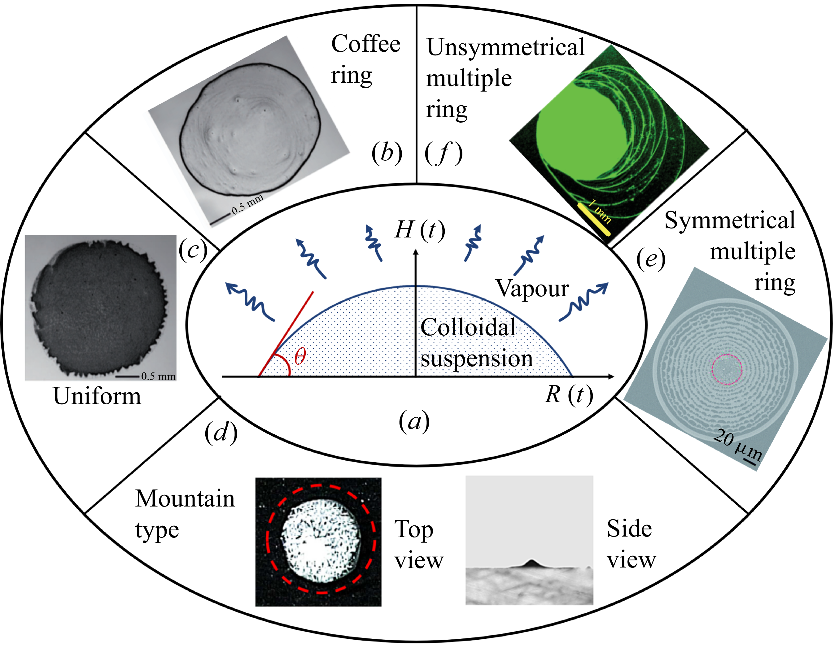
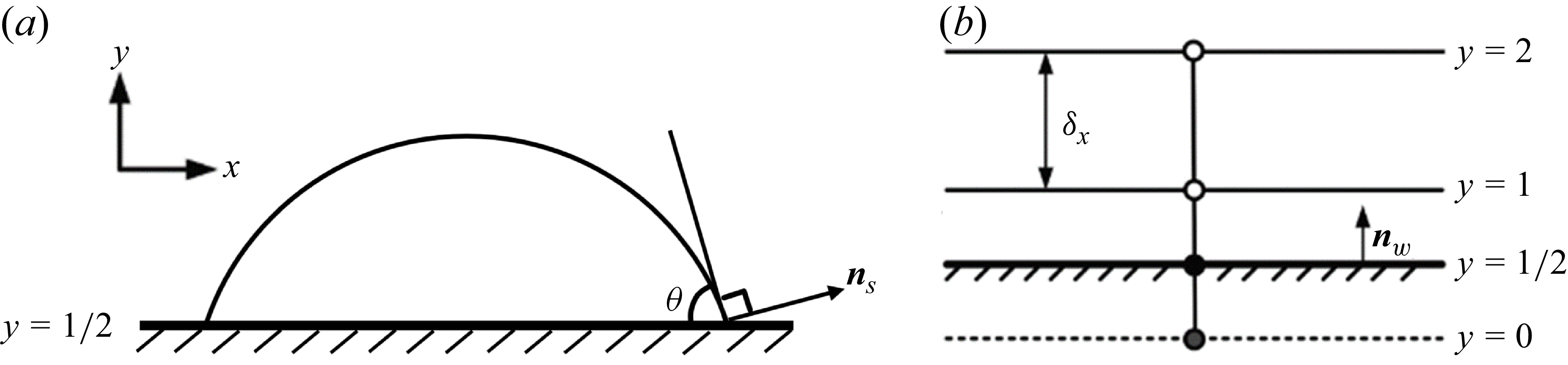


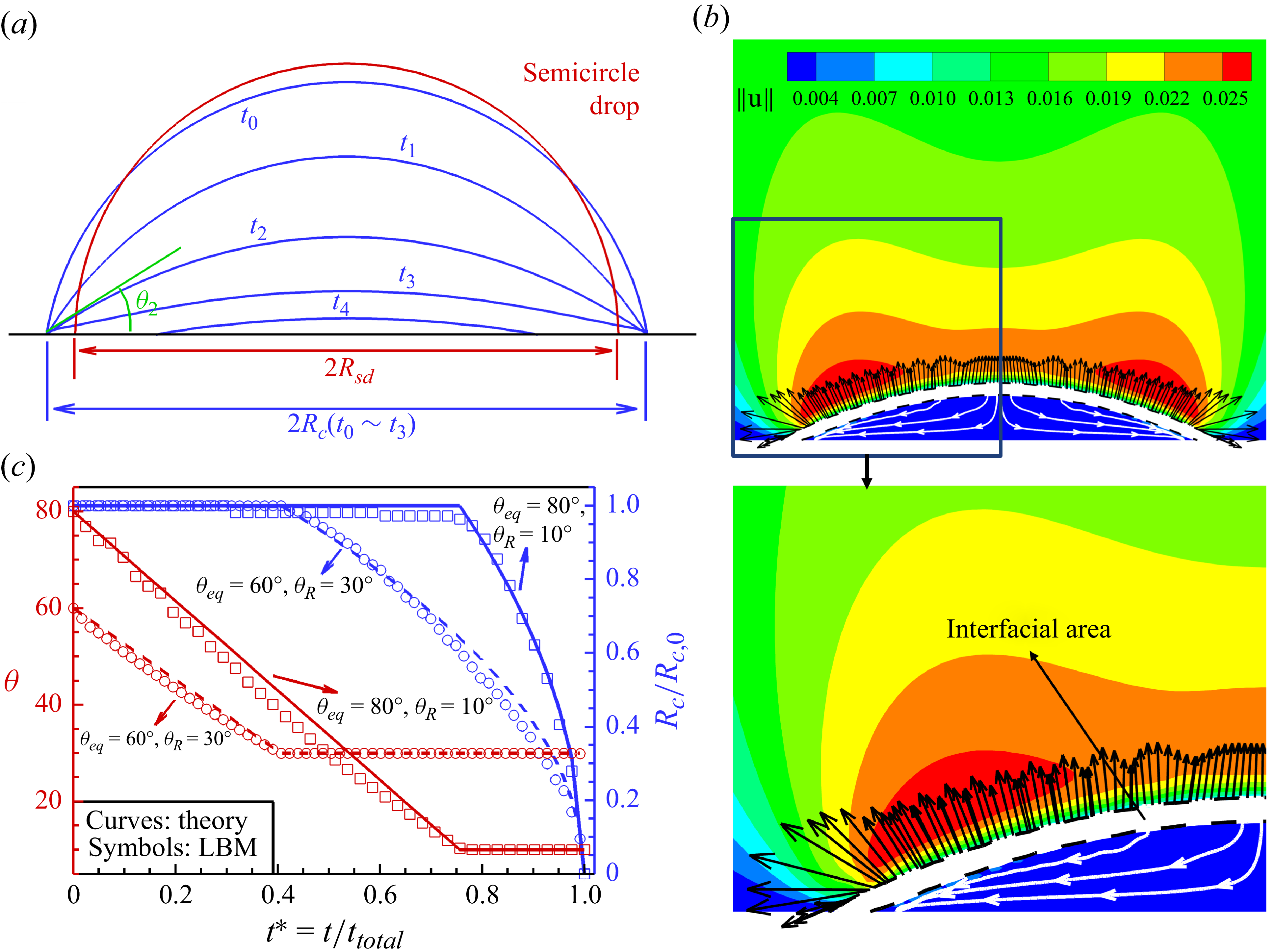


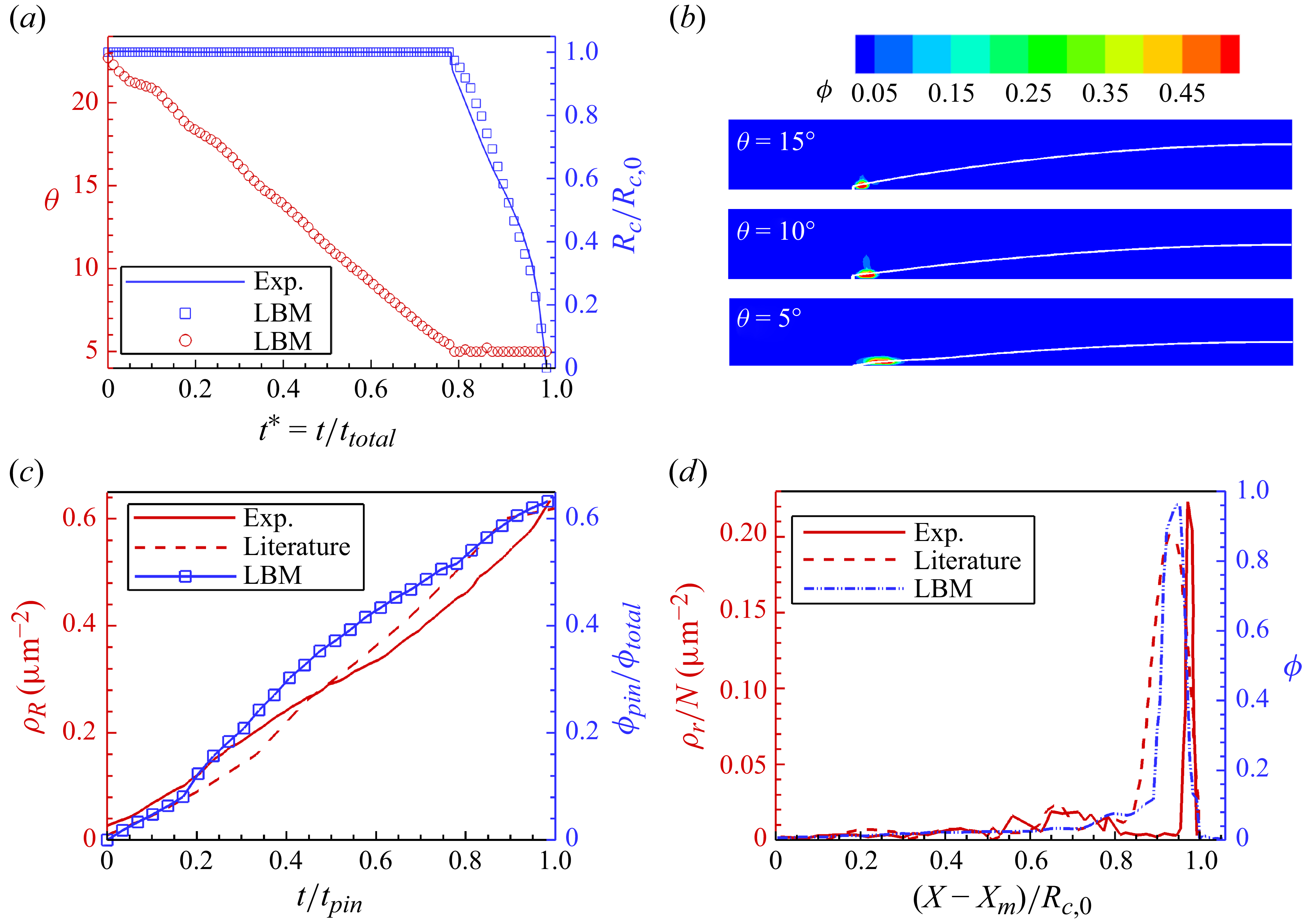


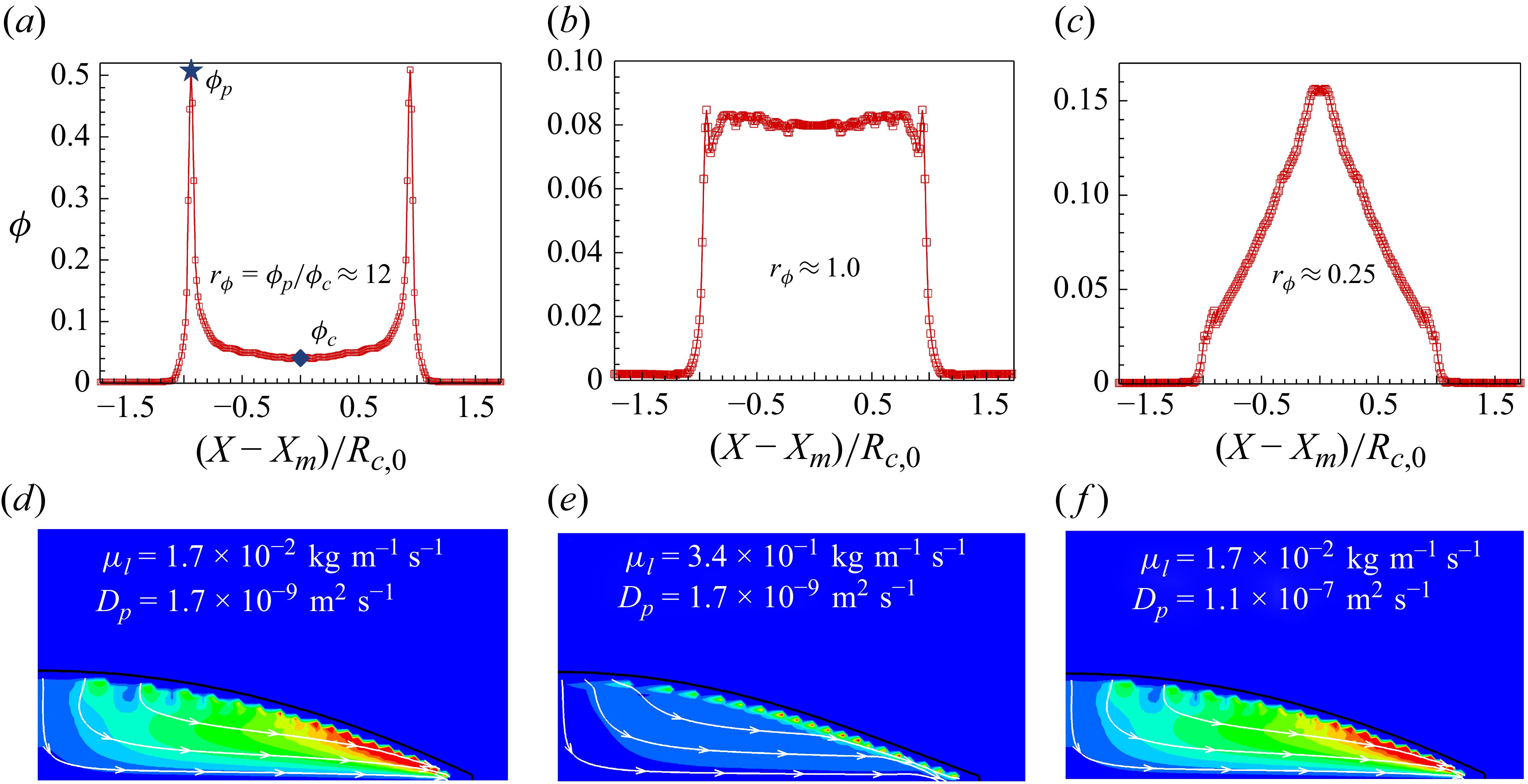


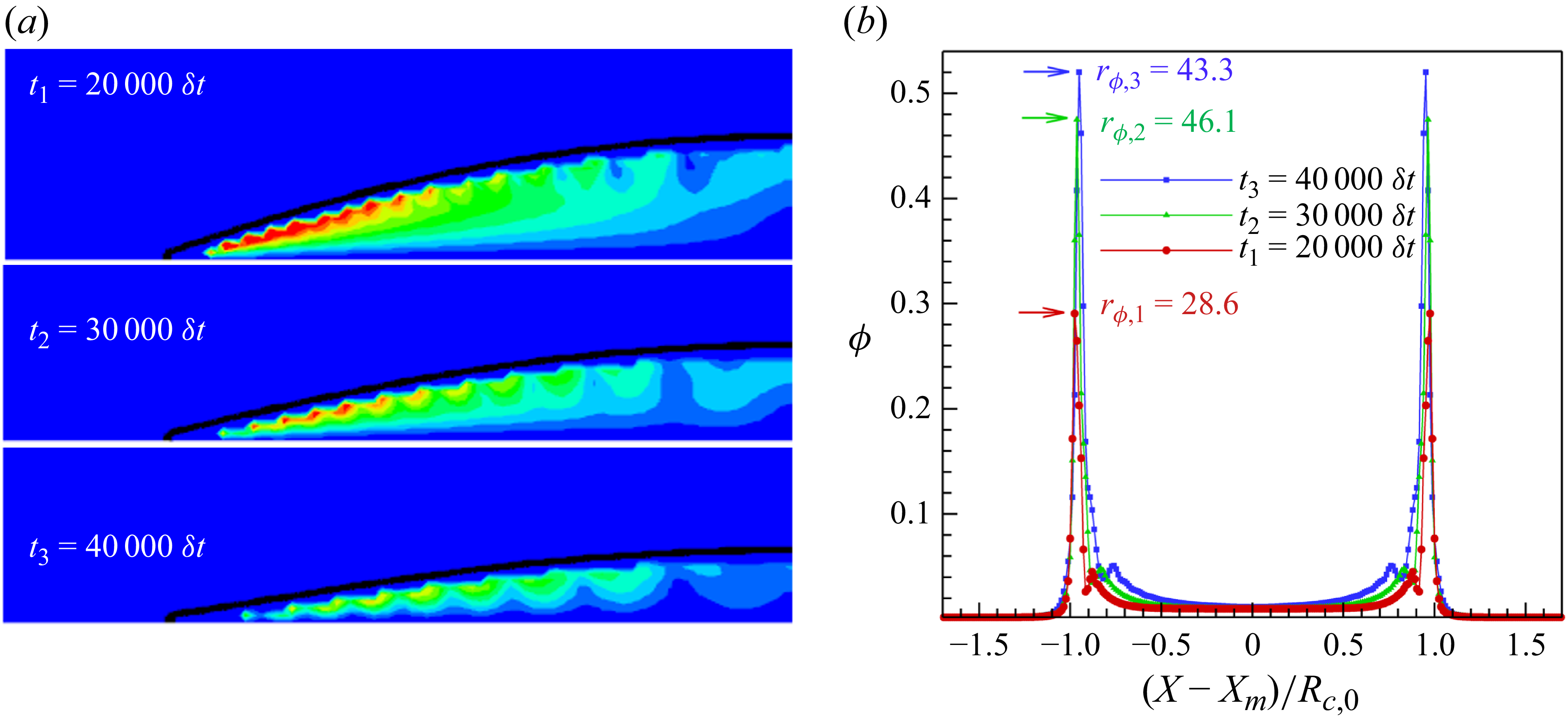
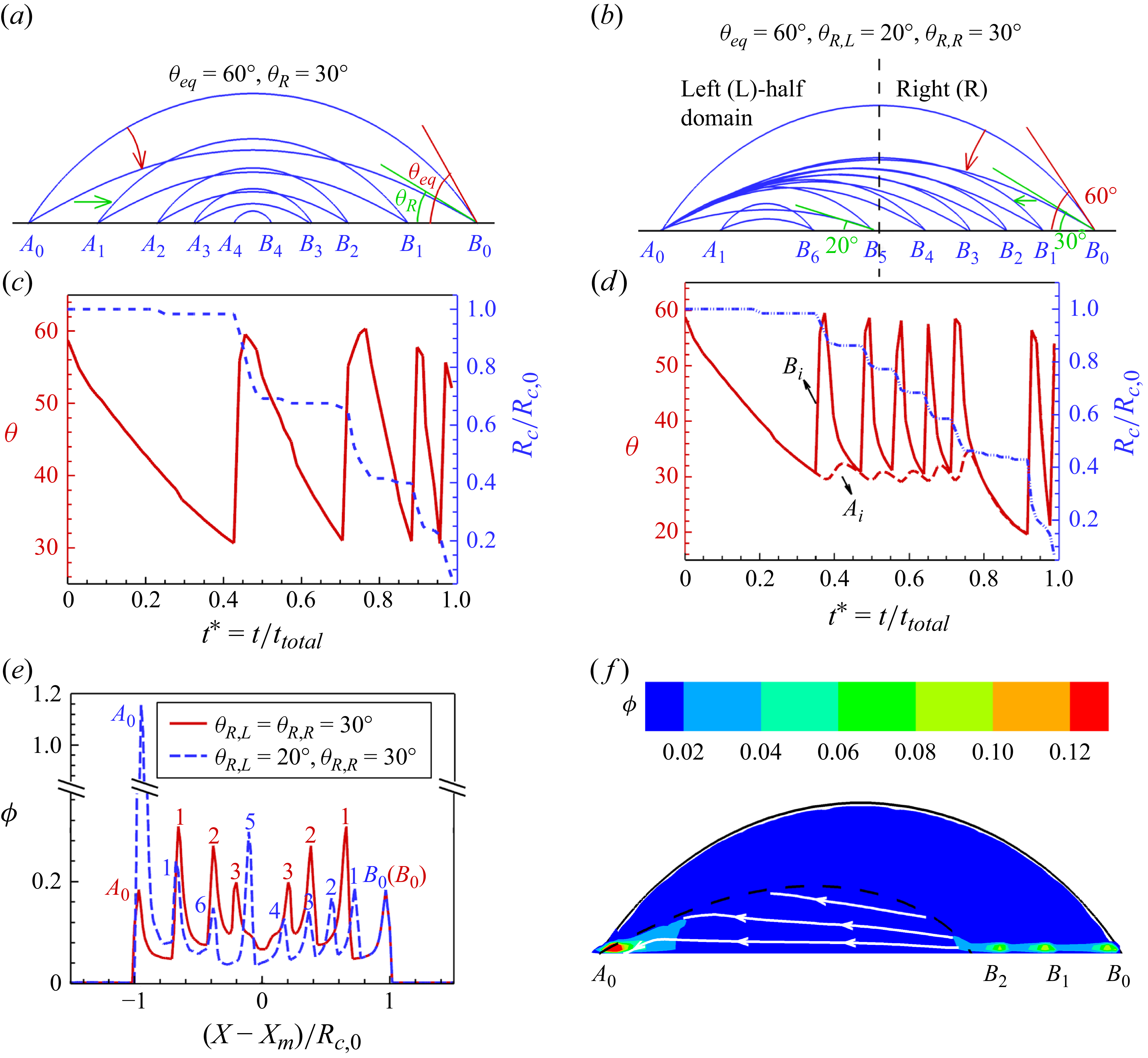


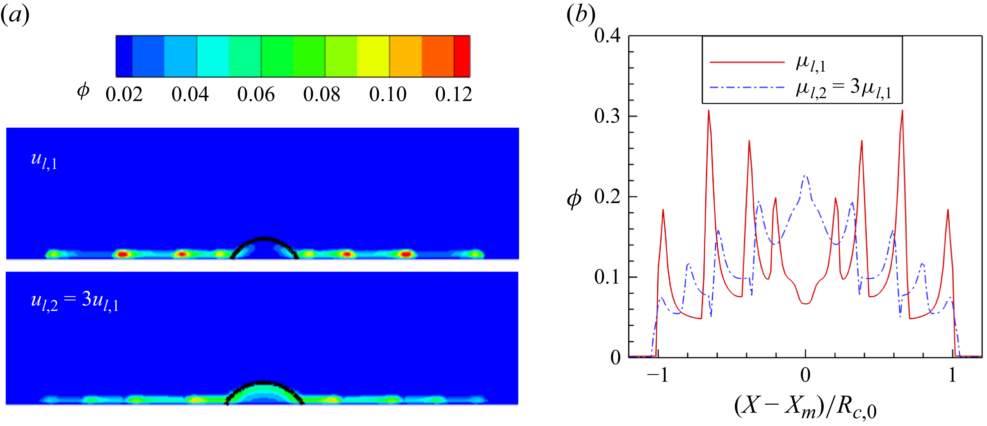
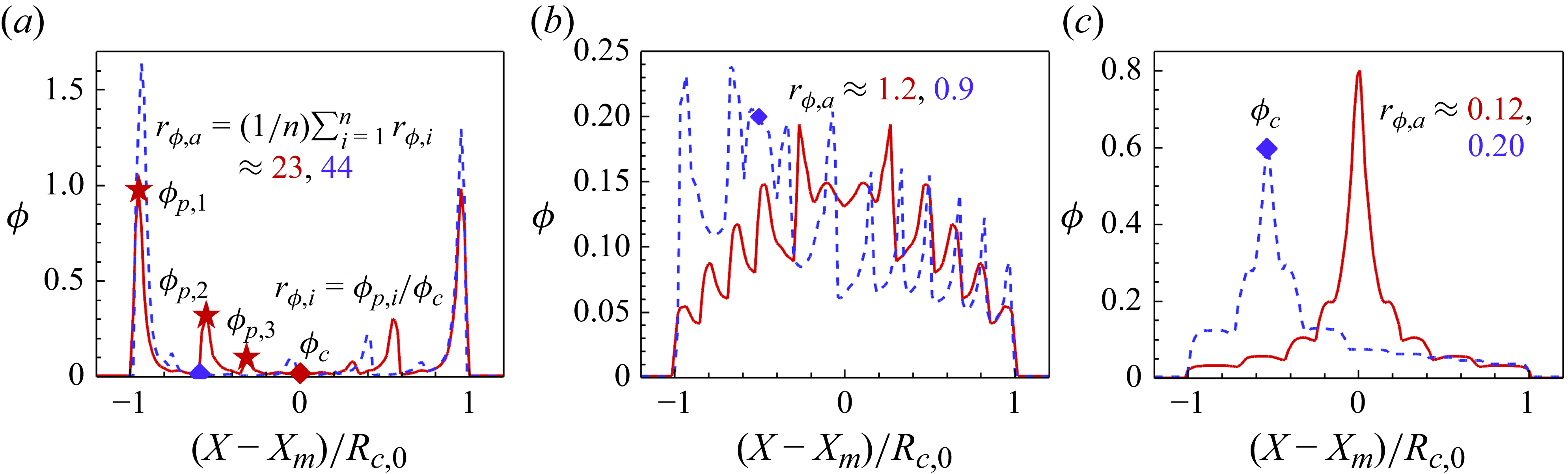


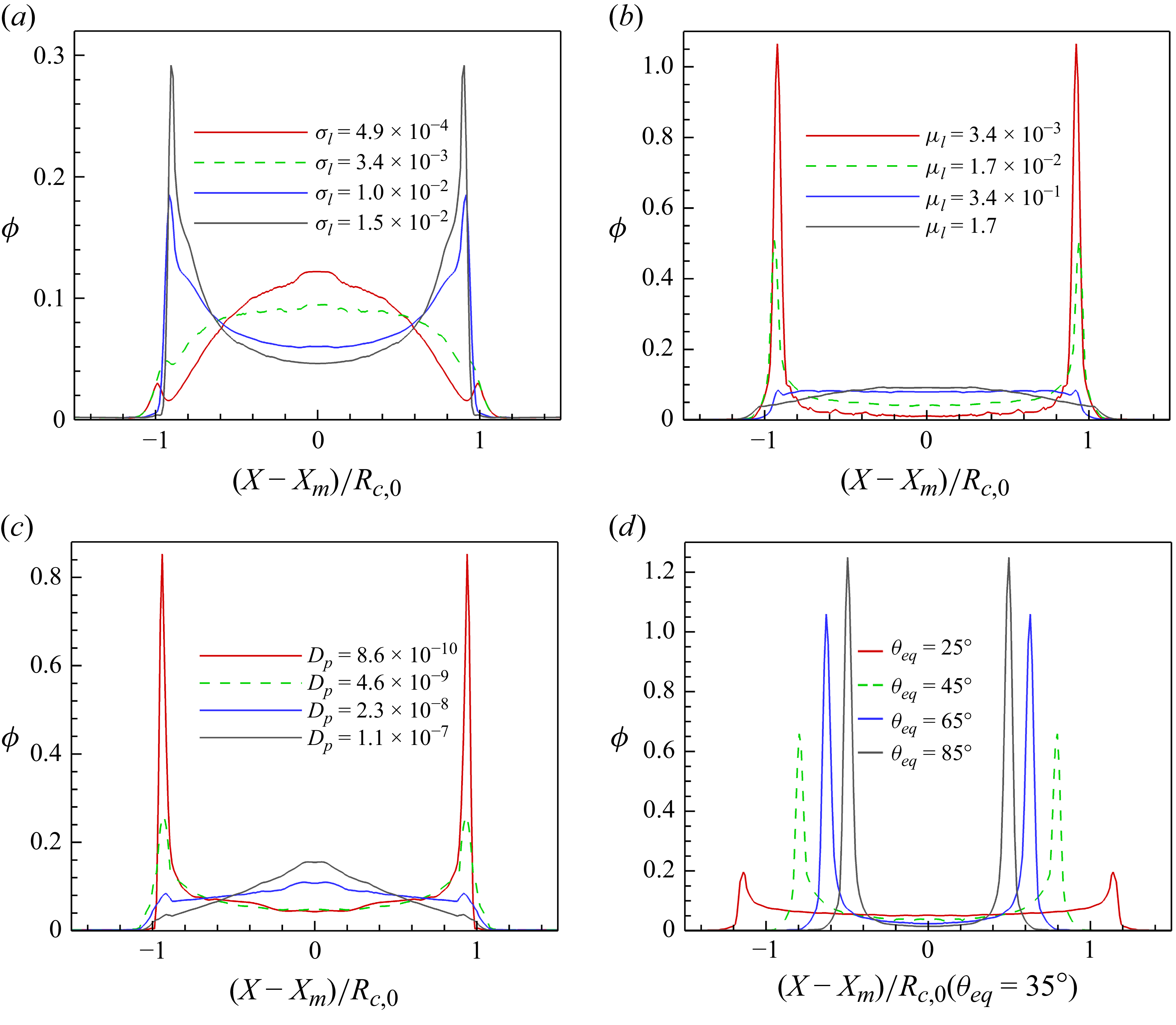


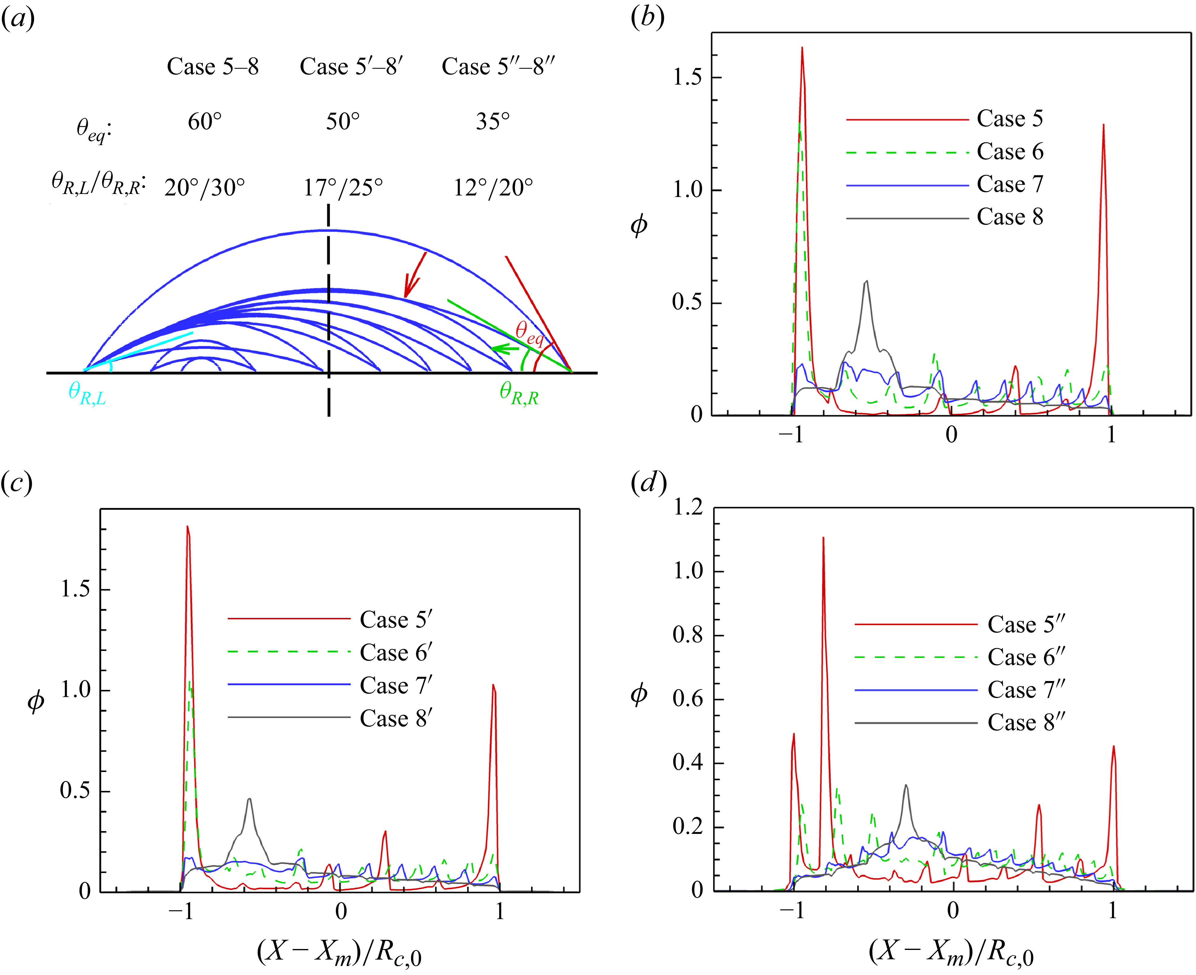


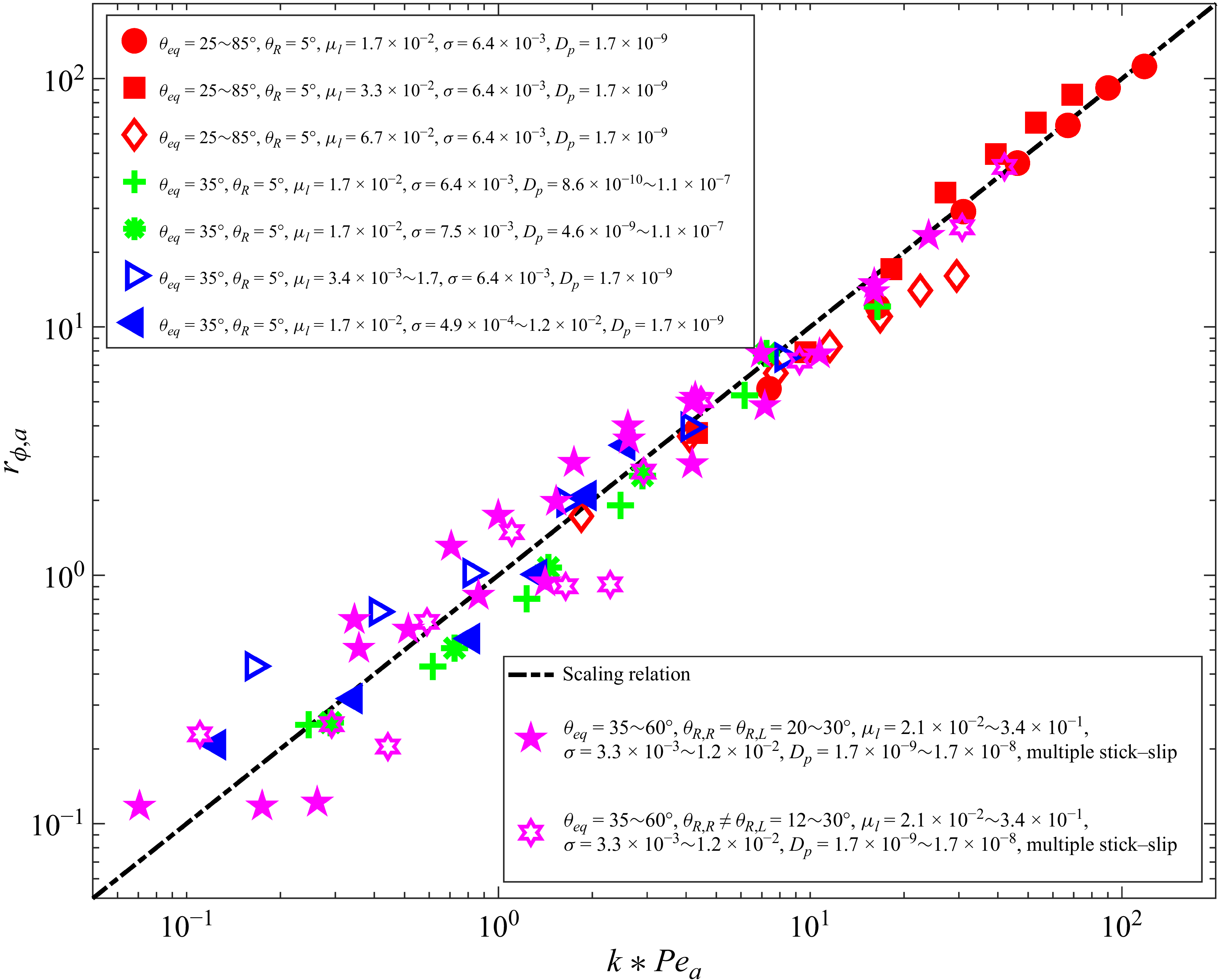


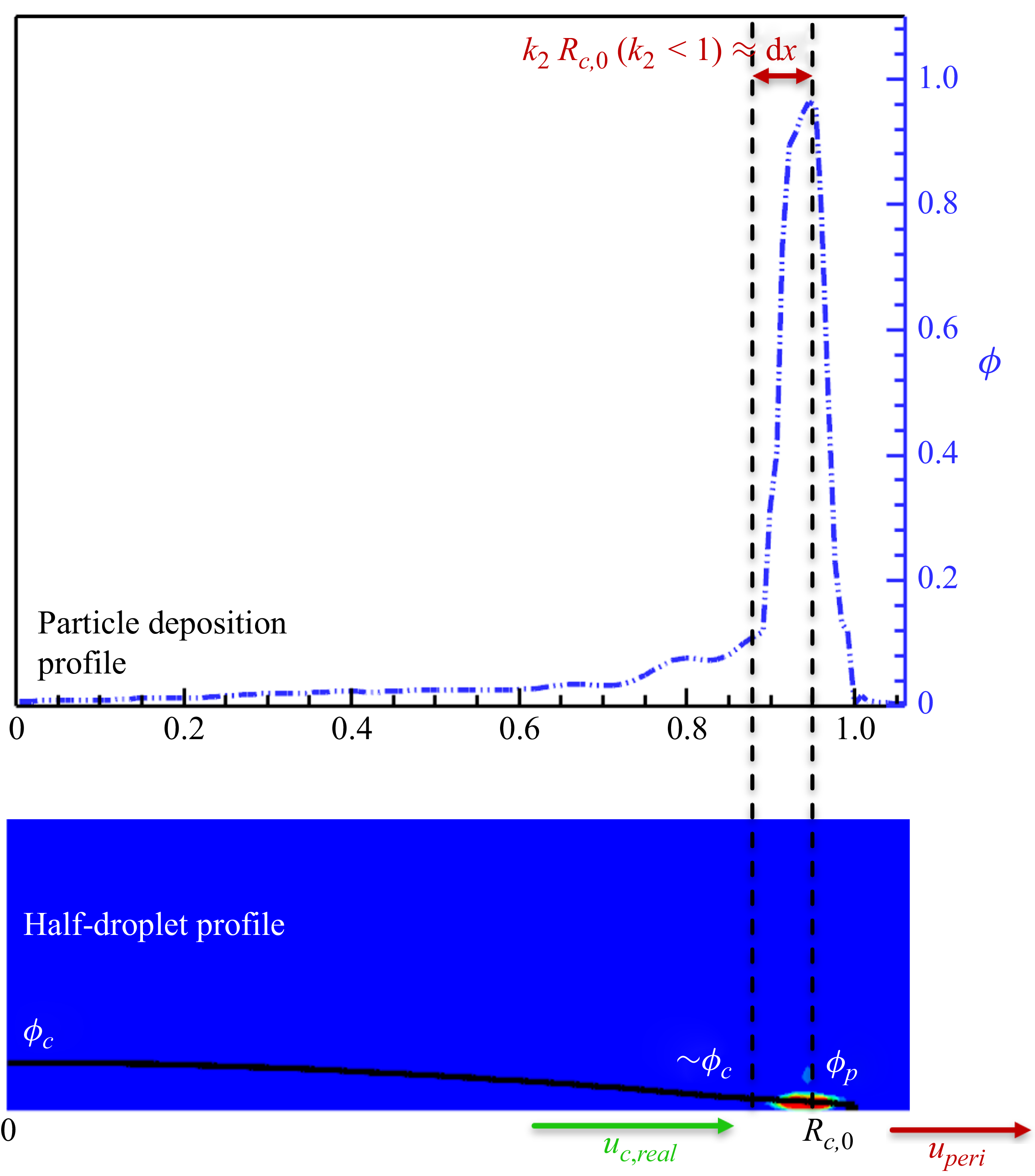
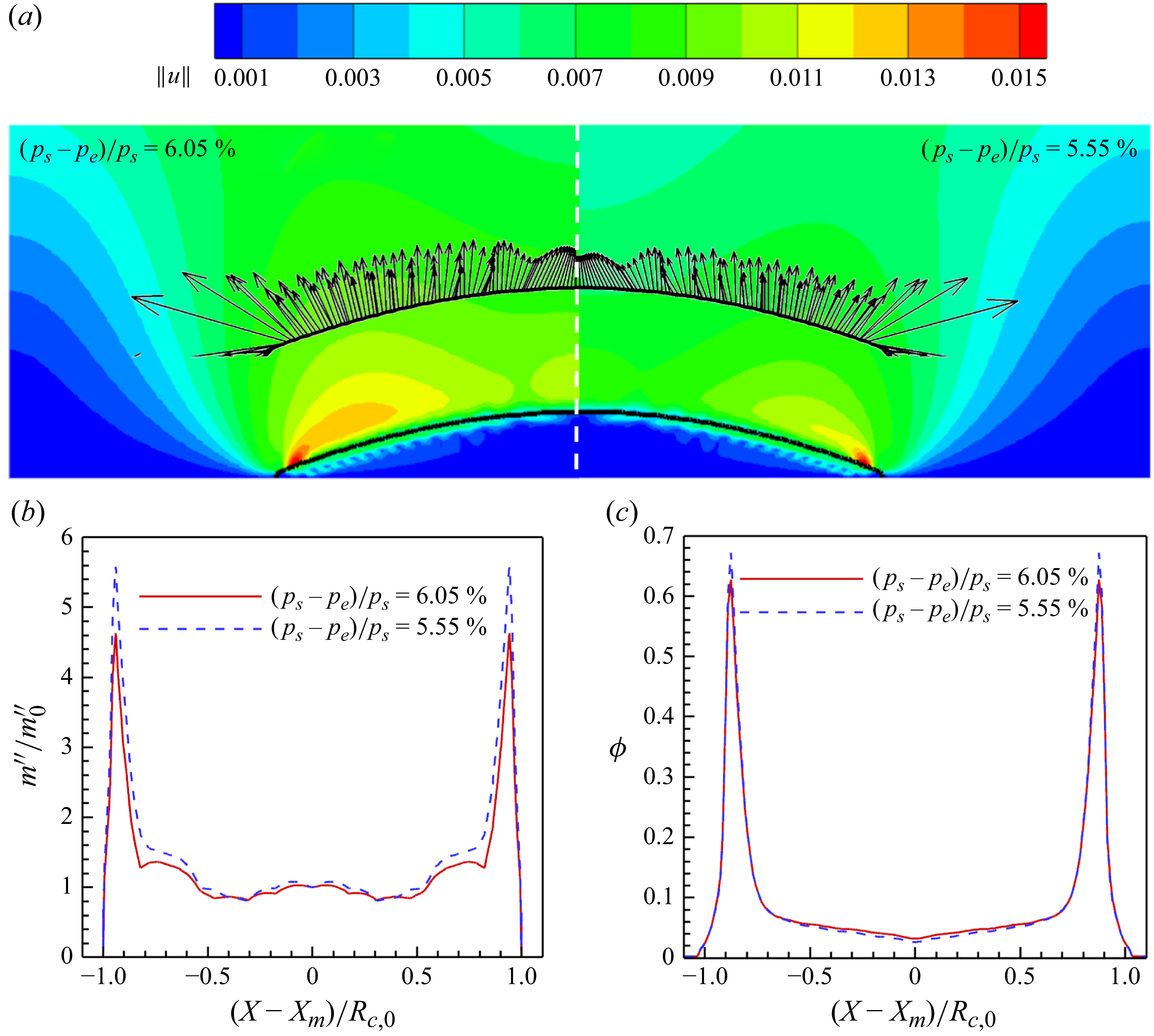


 Open access