





Introduction
South Florida has had a history of migration primarily from the US South and the Caribbean throughout its US history, but heightened movement over the past 70 years has resulted in a demographic shift that has completely changed the region’s culture, economy, and language. Although Spanish fluency in South Florida has greater economic power than in many other parts of the US, children who grow up in the region are still expected to primarily speak English. This expectation has resulted in a complex linguistic situation that reflects multiple types of language contact effects. Some adults may speak a mid-stage interlanguage if they have yet to gain English fluency. In some neighborhoods, entire communities have undergone a language shift from languages like Spanish and Haitian Creole to English. In other cases, the imposition (Van Coetsem, Reference Van Coetsem1988:11) from a home language may have created individual idiolects. Regardless of the reasons for variation, the adults in South Florida often speak different varieties of English from one another and children in South Florida must navigate this linguistic variation.
The dissertation this paper stems from aimed to understand social group dynamics, systemic hierarchies, and related language variation in pre-adolescents at a South Florida middle school (Sims, Reference Sims2021:11-14). In the dissertation, some linguistic variables (e.g., third singular -s and /ai/ trajectory length) varied predictably based on social factors like social group affiliation and interview setting (Sims, Reference Sims2021:222-237). For reasons that will become clear, to best understand why and how the socially conditioned linguistic variation exists in this community—discussed in other work (Sims, MS)—we must first establish that extensive variation exists that is not socially predictable. The variables discussed in this paper (i.e., /o/ trajectory length; /o/ place; /æN/; and /æ/ place) had high amounts of variation, but the variation was not socially predictable (Sims, Reference Sims2021:193-205). This paper focuses on the variables that did not vary socially to argue that South Florida is undergoing a process of dialect creation called new-dialect formation. The term new-dialect formation is applied to situations in which mutually intelligible dialects come into contact to create a new variety of the same language via a process of koineization; I abbreviate this term to NDF in the remainder of this paper to hopefully make clear the distinction between this specific process and dialect formation in general. In cases of NDF, high variability leads to accommodation and eventual dialect leveling.
I use child speech data to argue that the English of South Florida is undergoing the three-stage process of NDF as outlined by Trudgill (Reference Trudgill2004:28-38). Although this case differs from canonical examples of NDF because most of the varieties coming into contact are not dialects by the strictest definitions, the same processes of accommodation, leveling, simplification, and reallocation are occurring. In this paper, I: describe the sociohistorical and linguistic context of South Florida, then review literature related to dialect creation generally and NDF specifically; describe the goals of this project and discuss the relevant data collection, processing, and analysis methods; present the results of the statistical models; and conclude by discussing how this evidence supports the NDF claim.
Background
South Florida context
After the US acquired Florida from Spain in 1819, northern Florida was characterized by large cotton and sugar plantations similar to neighboring Georgia and Alabama (Florida Memory, n.d.), but southern Florida was mostly wilderness, Seminole territory, and military forts until Dade County (which included current-day Miami-Dade, Broward, and Palm Beach counties) was created under the 1835 Territorial Act. Early movement into the region, prompted by the 1862 Homestead Act, and subsequent building of infrastructure (Bowman & Forde, Reference Bowman and Forde2018; Rivers & Brown, Reference Rivers and Brown1996), likely caused considerable dialect mixture. The earliest settlers with US origins migrated from Northern Florida and Georgia (Rivers & Brown, Reference Rivers and Brown1996), with smaller numbers from other areas in the US South and beyond. Bahamians moved primarily into the incorporated community of Coconut Grove to take advantage of the cheap land, and African Americans from the US South were transported into the region via convict leases to build a railroad to accommodate these new populations (Bowman & Forde, Reference Bowman and Forde2018). The varieties that developed in this early period were likely interesting from a contact perspective, but are much less critical to the discussion at hand than those that have developed since a large population shift that began occurring in the late 1950s.
In 1960, the Hispanic population of Miami-Dade County was around 5%; by 2000, the population was 57% (Stephen P. Clark Center, 2003). The Cuban revolution and related mass immigration of the Cuban elite began in 1959 (Grenier & Castro, Reference Grenier, Castro and Jones-Correa2002). Typically, immigrants to the US are expected to assimilate seamlessly into the fabric of society; however, in South Florida, this was not the case because of the upper-class status and exile mindset of early Cuban immigrants (Mohl, Reference Mohl1985). Their class allowed them to influence policy during the 1960s and rise to power politically themselves in the 1970s and 1980s (Mohl, Reference Mohl1985; Stepick et al., Reference Stepick, Grenier, Castro and Dunn2003:1-33) with five Cuban mayors across municipalities in Miami-Dade County and seven Cuban congressmen in Florida by the early 1990s (Pérez, Reference Pérez, Grenier and Stepick1992). Their financial power allowed them to establish trade with South America and the Caribbean, changing the region’s economic landscape and providing a pathway to success for other Spanish-speaking immigrants (Grenier & Castro, Reference Grenier, Castro and Jones-Correa2002).
Hurricane Andrew in 1991 further changed the region’s demographics; after many homes were destroyed, 28% of the southern Miami-Dade County population relocated, at least temporarily (Girard & Peacock, Reference Girard and Peacock1997), to other parts of Florida or out of state (Smith & McCarty, Reference Smith and McCarty1996). Of the 40,000 people who permanently moved from the area (Smith & McCarty, Reference Smith and McCarty1996), proportionally, the Anglo-white population was least likely to return (Girard & Peacock, Reference Girard and Peacock1997), irreversibly altering the region’s ethnoracial demographics.
Among the racially Black population, there has not been as much exodus, but there has beensignificant influx. Most notably, mass Haitian immigration to the US began after a change in government structure in the late 1950s, though their numbers to South Florida were smaller until the 1970s through the 2000s (Mohl, Reference Mohl1985; Stepick, Reference Stepick, Grenier and Stepick1992; Wah, Reference Wah2013).
Other political incidents and environmental disasters have created a near-constant influx of immigrants from primarily Caribbean locales, which has resulted in clear evidence of language contact on the English varieties spoken in the region. Most of the research thus far has focused on the direct effects of contact, like imposition in bilingual speech. Transfer from Spanish has been noted in the lexicon (Carter & Merii, Reference Carter and Merii2023) and phonology (Carter et al., Reference Carter, López Valdez and Sims2020) of the English spoken by bilingual, first- and second-generation HispanicsFootnote 1. Within morphosyntax, the speech of a South Florida Haitian American differed from varieties of African American English (AAE) spoken in other US regions (Rickford & King, Reference Rickford and King2016). There is also evidence for change beyond direct imposition. The phonological effects on the vowels and prosodic rhythm for Spanish-English bilinguals significantly varied based on their reported rates of Spanish use (Sims & Austen, Reference Sims and Austen2018), but the prosodic rhythm of Haitian Americans did not (Sims, Reference Sims2025). Among non-bilingual populations, Anglo-white Miamians differed in prosodic rhythm based on the proportion of Hispanics in the neighborhood they grew up in (Enzinna, Reference Enzinna2016). The degree to which the variation found in these past studies is particular to individual or social group speech patterns, common across bilinguals, or characteristic of South Florida speakers in general has yet to be established.
In the dissertation, I aimed to tease apart some of the social reasons for the variation in the region. I found that some variables were socially predictable, for example, the “nerds” had longer /ai/ trajectory length before voiced consonants than members of the other social groups (Sims, Reference Sims2021:226). But I also found that other variables were not predictable by social situation, for example, /o/ trajectory length (Sims, Reference Sims2021:195-197). Despite not being predictable, though, individuals still had different trajectory lengths (Sims, Reference Sims2021:197). In this paper, I concentrate on the variables that did not vary socially to establish the dialect creation process(es) at play before examining the social implications in subsequent work (Sims, MS).
Dialect creation and change
Migration and mobility are often catalysts of language variation and change, so studies of dialect creation and change via contact are common. While aspects of many processes of dialect creation are present in the South Florida linguistic situation, none fully explains the changes seen.
For the past decade, sociolinguists have described South Florida linguistic phenomena primarily focusing on the speech of Hispanics with varying degrees of bilingualism; from this work, scholars have drawn the conclusion of an emerging Hispanic ethnolect (e.g., Carter et al., Reference Carter, López Valdez and Sims2020). Ethnolects can develop because of language shift within immigrant populations. For example, the imposition of intonation from Yiddish onto English results in the prosody associated with the Jewish English ethnolect (Burdin, Reference Burdin2016:183-188). These varieties are then perpetuated because of identity and social segregation.
Relatedly, multiethnolects, new varieties of the majority language used across minority ethnic groups (Clyne, Reference Clyne2000), have gained a lot of traction in describing urban contact dialects in other cities (e.g., Multicultural London English: Cheshire et al., Reference Cheshire, Kerswill, Fox and Torgersen2011). In contexts of multiethnolectal formation, people migrate into urban neighborhoods from countries that speak other languages and negotiate a new dialect of the majority language (Kerswill & Wiese, Reference Kerswill, Wiese, Kerswill and Wiese2022). The role of adolescent identity formation and youth styles is often emphasized as the catalyst to the creation of multiethnolects (e.g., Wiese, Reference Wiese2009),
Contact between dialects can also prompt change. For example, some mainstream varieties of Sydney English are becoming r-full when Australian English is historically thought to be r-less (Gibson et al., Reference Gibson, Penney and Cox2022) because of contact with a large multiethnolect developing in the city. There is a clear and direct path of change in mainstream Sydney English from a variety that is r-less to one that is r-full.
NDF occurs when speakers of mutually intelligible varieties come into contact and create a non-continuous new dialect. For example, New Zealand English was created from contact primarily between English, Irish, and Scottish settlers (Gordon et al., Reference Gordon, Campbell, Hay, Maclagan, Sudbury and Trudgill2004:36-52). There was not a fully predictable path of change from one dialect to New Zealand English; rather, the new dialect included features that were clearly from different dialects. The features in the new dialect reflected the demographic proportions of dialect speakers and subsequent frequency of linguistic variables (Trudgill, Reference Trudgill2004:26; Trudgill et al., Reference Trudgill, Gordon, Lewis and Maclagan2000). Contemporary work on NDF spans the globe; for example, in New York City, speakers of Spanish from different regions are negotiating a new variety of Spanish (Fernández-Mallat & Newman, Reference Fernández-Mallat and Newman2022). As another example, Pasifika English has been created by English-speaking Pacific Islander immigrants to New Zealand (e.g., Starks et al., Reference Starks, Gibson, Bell, Williams, Schneider, Trudgill and Schreier2015).
Cognitive and social processes like imposition, accommodation, and identity formation are apparent in all studies of new dialects to differing degrees, which makes it difficult to tease apart which specific dialect creation processes are at play in any given situation. I frame this study around NDF rather than ethnolects, multiethnolects, or a more general dialect change framework for three primary reasons. The first two reasons are deduced primarily based on past work and insights from the sociohistorical context; the final is evidenced by the analyses in this paper. First, NDF relies primarily on accommodation—the process by which speakers adjust their speech to match their conversation partners—rather than identity formation to explain the dialect formation; recall the variables discussed here were found not to vary based on social factors (Sims, Reference Sims2021:173-220), so they are unlikely to be extensively involved in identity formation. Second, there is no clear direction of change from one established dialect to this new one. There is little description of English in South Florida prior to the demographic shift in the mid-twentieth century—though in apparent time, the Atlas of North American English (Labov et al., Reference Labov, Ash and Boberg2006:242-257) may get close. Despite this lack of description, we can speculate that South Florida has also had a change in social capital and power dynamics that have changed the mainstream culture; the immigrant groups that are now in power in South Florida do not have established English dialects from which a direct path of change can be drawn. Last, and demonstrated the most directly by the linguistic evidence in this paper, the scale of language shift and subsequent sociolectal contact in South Florida is widespread rather than specific; the entire region is potentially affected, rather than a single group of minoritized people.
Linguistic variables
I examine four sets of variables (i.e., /o/ place; /o/ trajectory; /æ/ pre-nasal allophonic split; non-pre-nasal /æ/ place). Recall that these variables varied but did not vary for social factors like social group (Sims, Reference Sims2021:173-220). An alternate explanation for the variation is that it might stem from the imposition of Spanish or Haitian Creole—the most spoken languages in South Florida other than English (U.S. Census Bureau, 2015)—in the speech of bilinguals. If the variation we find is only seen in the bilingual population, we can conclude imposition is the only factor at play; if these variables differ within the monolingual population as well, perhaps a more complex explanation, like NDF, is warranted.
/o/ place
English, Spanish, and Haitian Creole all have an /o/ phoneme, but each respective /o/ is realized with slightly different F1 and F2 quality. There are other differences between the phonemes across the languages, like phonotactics and voice quality, but this paper focuses on the differences in F1 and F2 space. Because of the differences between languages, bilingual Haitian Creole/English children as young as five years produce English /o/ with a lower F1 than monolingual English-speaking children (Wallen & Fox, Reference Wallen, Fox, Levis and LeVelle2011). If imposition were a major factor in the language variation in the community, I would predict that the F1 of Haitian Creole bilinguals will differ from that of Spanish bilinguals or English monolinguals. As for F2, back vowel fronting has independently developed in numerous regions of the US (Thomas, Reference Thomas1989, Reference Thomas2001:28-32), though the fronting is often less pronounced in varieties of African American Language than in white varieties (Durian et al., Reference Durian, Dodsworth and Schumacher2010; Fridland & Bartlett, Reference Fridland and Bartlett2006; Thomas & Wassink, Reference Thomas, Wassink, Llamas and Watt2010). Similarly, Spanish /o/ has a lower F2 than English /o/, and there are differences between Spanish and English in F2 depending on the following environment (Bradlow, Reference Bradlow1995). Because of this, I expect Spanish bilinguals to differ from the other populations in F2 depending on the following environment, though differences within US English varieties may muddy evidence of this imposition.
/o/ trajectory
/o/ in US English is realized with on- and off-glides that create a diphthong-like quality in many communities (Lehiste & Peterson, Reference Lehiste and Peterson1961) (e.g., /o/ in goat [goʊt]). /o/ is a simple vowel in both Haitian Creole and Spanish. I expect shorter /o/ trajectories in bilingual speakers than monolingual English speakers of any ethnicity due to imposition from their other languages. I do not expect variation in /o/ trajectory within the speech of monolingual English speakers.
/æN/
Of the most common languages spoken in South Florida, /æ/ is a phoneme only in English. In Mainstream US Englishes, /æ/ raises and tenses before nasal consonants (Thomas, Reference Thomas2001:19-23), but there is a well-documented reduction of the /æN/ split in varieties developed via contact with Spanish. Chicano English did not have the degree of /æ/ raising/tensing as white California English (Fought, Reference Fought2003:62-92); Mexican Americans in Raleigh and South Texas resisted the /æN/ split as well (Thomas et al., Reference Thomas, Carter and Coggshall2006). In Washington, DC, the distance between the allophones was shorter in Latino speech than in European American speech for those who learned English as children (Tseng, Reference Tseng2015:115-127). In South Florida, Hispanics who used Spanish in a variety of situations (i.e., not only at home with their parents) had less distance between their /æN/ and other /æ/ tokens than those who reported using Spanish less often (Sims & Austen, Reference Sims and Austen2018); there was no correlation between other aspects of the participants’ ethnic identities pointing specifically to phonological imposition for this variable.
/æ/ place
Also in South Florida, /æN/ was produced more toward the front of the mouth and at a higher point in Anglo-white participants than among Latinx participants (Carter et al., Reference Carter, López Valdez and Sims2020). The Latinx /æ/ was produced significantly further back than the /æ/ of the Anglo-white participants. This did not show a lack of allophonic split, as in past studies of Hispanic varieties, but in general, Latinx /æ/ was produced closer to the typical /ɑ/ space. An exploration of /æN/ would be enriched by a comparison to /ɑ/. I expect Spanish bilinguals to have either a shorter distance between /æ/ allophones than non-Spanish speakers, an /æ/ near the place of /ɑ/, or a combination of the two.
Child speech in NDF
Systematic studies of child speech in ongoing situations of language contact are rare (Kerswill et al., Reference Kerswill, Cheshire, Fox, Torgersen, Schreier and Hundt2013); nonetheless, research suggests that young children (before age six) speak the varieties their caregivers speak, and preadolescents (ages 6-12) have reoriented to the speech of their peers (Kerswill et al., Reference Kerswill, Cheshire, Fox, Torgersen, Schreier and Hundt2013). This well-cited sociolinguistic expectation of child speech (e.g., Trudgill, Reference Trudgill1986:31) is expressly present in language contact situations, such as the one in South Florida, in which children are born into communities with adults who speak numerous dialects (Kerswill et al., Reference Kerswill, Cheshire, Fox, Torgersen, Schreier and Hundt2013). In situations of NDF, there is no clear prestige variety, so a “tabula rasa” situation arises in which the competing features of the distinct dialects are leveled, simplified, and reallocated over time (Trudgill, Reference Trudgill2004:26-30). This process is thought to occur in three stages: (1) mixing and individualized accommodation; (2) extreme intra- and interpersonal variability with some leveling of marked features; and (3) a focused dialect emerges (Trudgill et al., Reference Trudgill, Gordon, Lewis and Maclagan2000). The reduction of these features across the three stages of NDF is facilitated by children who need to learn to speak in the environment of dialect mixture (Trudgill, Reference Trudgill1986:28-38) and who have more flexible accommodation strategies than adults (Trudgill, Reference Trudgill1986:31). As such, this paper makes use of child speech data. Variation in the adult population can, presumably, best demonstrate how advanced the dialect creation process was when they were young, rather than the stage the region is currently in.
Many studies of NDF have relied on evidence collected after the dialects were established rather than as they were developing (Kerswill & Williams, Reference Kerswill and Williams2000:67). For examples of NDF that developed far in the past, concrete evidence of characteristic second-stage mechanisms has been elusive, since the children critical during this stage did not create many written records with which to explore the creation in progress (Trudgill, Reference Trudgill2004:100). Studies of NDF in immigrant languages that have been conducted with adult speakers have allowed researchers to speculate on the role of children in NDF a bit more concretely with the inclusion of targeted questionnaires (e.g., Fernández-Mallat & Newman, Reference Fernández-Mallat and Newman2022). The inclusion of 4-, 8-, and 12-year-olds in a study of the Milton Keynes dialect is a notable exception to the norm of relying on adult speech to confirm NDF hypotheses; it concretely established that children are indeed responsible for the emergence of new dialects at least in the realms of phonology and morphosyntax (Kerswill & Williams, Reference Kerswill and Williams2000) whereas adolescence may be a key site for pragmatic negotiation (Fernández-Mallat & Newman, Reference Fernández-Mallat and Newman2022). Lastly, child speech in multi-ethnic environments differs from child speech in situations of mono-ethnic dialect contact (Cheshire et al., Reference Cheshire, Kerswill, Fox and Torgersen2011), which may have implications for NDF.
This paper was not designed to be a systematic study of NDF in youth communities, but because of the importance of children in dialect leveling in NDF, this analysis of child speech can still shed light on which stage of NDF South Florida is currently inhabiting.
Summary and aims
The history of South Florida demonstrates that it is a ripe environment for contact effects. Work in other cities has demonstrated the mixture of immigrant Englishes with established local varieties to create new neighborhood varieties (e.g., Cheshire et al., Reference Cheshire, Kerswill, Fox and Torgersen2011), but the population disruption and redistribution of power in South Florida may have prompted a “tabula rasa” situation that persists through geographic areas and economic classes. Because this migration has been continuous, contemporary children are likely learning English from adults who speak very different varieties of English; these varieties may be monolingual regional US dialects, ethnolects, bilingual varieties, or learner varieties. Most importantly, I expect the sheer number of varieties these children need to navigate will affect their speech.
The variables I explore in this paper did not vary based on social factors (Sims, Reference Sims2021:173-220), though each has been shown in other contexts to differ between monolinguals and bilinguals due to imposition. In this paper, I first aim to show that South Florida is currently undergoing a process of NDF rather than some other dialect creation process. I then argue specifically that South Florida is in mid-stage two of NDF in which children navigate the high variation of the community by themselves, having high levels of inter- and intraspeaker variation, but are beginning to show awareness of this variation and begin to level. To this end, I examine linguistic data collected from a South Florida middle school during the 2019-2020 school year.
Methodology
Data collection and processing
Most of the students and teachers at the middle school were, in order of most numerous, US-born and racially Black of any ethnicity, Haitian-born and racially Black, and HispanicFootnote 2 with recent immigration from the Caribbean and Central America. Combined, the racially Black population made up 71% of the student body in the 2019-2020 school year, another 25% were Hispanic, and 3% were of mixed racial ancestry (NCES, 2023). The school population was not representative of the zoned neighborhoods since middle-class families often opted for private or charter schools instead. For example, a middle-class neighborhood zoned for the school was 40% white non-Hispanic (U.S. Census Bureau, 2020) despite no white students attending the school; because of this, the students at this middle school likely have contact with a wider array of races and ethnicities outside of school.
Participants were collected via a combination of targeted recruitment and the snowball method. The data collection method was appropriate for the ethnographic goals of the dissertation for which they were collected, but, as a result, the sample is not representative of the school or community populations. Since the data were not designed with this paper’s specific NDF question in mind, the results are likely not very robust on their own. Other work stemming from the same dataset includes qualitative and quantitative analyses of linguistic and social phenomena that build on and support the preliminary hypotheses in this paper; future studies designed to test this hypothesis will also be needed.
The data analyzed here are audio-recorded interviews recorded using a Zoom H4 recorder with a 44.1 kHz sampling rate to collect interview data. Participants were recorded either one-on-one, with a group of their peers, or with a group of their closest friends in semi-structured interviews and open-ended ethnographic interviews. I have around 22 hours of audio-recorded data from 72 interviews that ranged from seven to 51 minutes each. All participants who were interviewed, except for a participant with a speech issue and participants with only a few minutes of recorded data, are included in the interspeaker analysis. There is data from 32 participants (22 female, 10 male) across 29 interviews. Each participant was in sixth grade, and their ages ranged between 11 years five months and 13 years four months at the time of the interview.
I transcribed using ELAN (Wittenburg et al., Reference Wittenburg, Brugman, Russel, Klassmann and Han2006) with the help of two research assistants. For interviews with messier audio, I analyzed only sections without overlap. Force-alignment was done via FAVE-Align (Rosenfelder et al., Reference Rosenfelder, Fruehwald, Evanini, Seyfarth, Gorman, Prichard and Yuan2014). I extracted F1 and F2 measurements of each token at five intervals (i.e., 20%, 35%, 50%, 65%, and 80%) (Fox & Jacewicz, Reference Fox and Jacewicz2017) using FAVE-Extract (Rosenfelder et al., Reference Rosenfelder, Fruehwald, Evanini, Seyfarth, Gorman, Prichard and Yuan2014) to minimize researcher judgment errors and ensure exact measurements at consistent intervals on the uncorrected TextGrids.
To test whether the uncorrected TextGrids were sufficiently accurate for analysis, I hand-corrected the segment boundaries of two interviews using the vowel boundaries described by Peterson and Lehiste (Reference Peterson and Lehiste1960). I extracted the formant measurements for the corrected and uncorrected interviews, then conducted Tukey tests on the Hz values of F1 and F2 of /æ/ tokens to determine potential outliers. Outliers in a Tukey test are defined as any values more than 1.5 times the interquartile range (Tukey, Reference Tukey1977). Outliers in this dataset could be due to predictable speech variation, but in the uncorrected measurements, they could also stem from TextGrid misalignment. A two-sample t-test found no significant difference between the mean outlier rates of the corrected or uncorrected TextGrids (t (5.54) = 0.4531, p = 0.66). There were differences in the number of tokens between the corrected and uncorrected datasets (e.g., Participant 69’s corrected token count was 93, and uncorrected was 85). Rather than giving wildly inaccurate formant values, FAVE-Extract omitted clearly misaligned tokens, which may explain the lack of a significant difference in the outlier rate. This data loss was deemed acceptable due to the large token counts in each interview.
Studies have shown significant differences between male and female children in F1 and F2 measurements in preadolescence (Bennett, Reference Bennett1981), and there are large drops in formant values due to puberty between the ages of 10-12 in girls and 14-15 in boys (Vorperian & Kent, Reference Vorperian and Kent2007; Vorperian et al., Reference Vorperian, Kent, Lee and Bolt2019). To account for these potential differences, I used the Lobanov (Reference Lobanov1971) normalization method in the phonTools R package (Barreda, Reference Barreda2015) since it was shown to minimize variation due to physical size but keep variation due to sociolinguistic factors (Kohn & Farrington, Reference Kohn and Farrington2012). Participants’ data had minimal, if any, changes due to aging, likely because only four months passed between the earliest interviews and the last. Regardless, I normalized each participant’s interview separately; for example, I grouped and normalized the tokens from Participant 54’s January interview separately from his March interview to account for potential growth. Each token was coded for social and linguistic variables.
Social variables
The larger research questions of this work surrounded identities, social groups, and interaction types, but the social variables did not account for the variation found in these linguistic variables (Sims, Reference Sims2021:222-237). Given this paper’s focus on variation that may stem from language contact, though, I include two social variables related to the participants’ home language: SpanishFootnote 3 and Haitian Creole. These variables had two levels, no or yes, indicating whether the language in question was spoken in the home. I include these measures to rule out imposition as the sole cause of the interspeaker variation found in these data; if the variables are significant, then it is possible the variation is just the result of individual bilingualism, not a larger process of dialect creation or change.
Linguistic variables
Each linguistic variable was coded for some or all of the following dependent variables: F1 and F2 at 20%, 50%, and 80% in Hz (e.g., F1.50, F2.80, etc.) and unscaled Lobanov normalization (e.g., F1.50.norm), and Euclidean Distance. Additionally coded were the specific Vowel, Target Word, Following Voicing, and Following Nasal, since all have been shown to affect vowel place, though not all were relevant to all analyses. I originally included Following Manner (stop, fricative, nasal, lateral, and other), but the dataset’s uneven token counts and frequent repetition of the same words meant that the Following Manner levels covaried with Following Voicing, so I used the simpler Following Nasal instead.
I used a series of linear mixed effects regression (LMER) models for the interspeaker and intraspeaker analyses. Each interspeaker model had random effects for Participant, to account for differences like token counts across speakers, and Word, to account for lexicalized variation. Since the data stemmed from naturalistic, uneven data sets, there was not enough data to account for all possible linguistic causes for variation. In addition, there was insufficient data to include random slopes. Future study is needed with a larger, more representative sample to account for allophonic and durational differences that are not directly related to the research question. The social factors Haitian Creole and Spanish were explored in each interspeaker analysis.
Other social factors were not included in these analyses for two reasons. First, previous work (Sims, Reference Sims2021:173-220) showed no relationship between these linguistic variables and social factors like gender, social group, and race. Second, some social factors required more complex coding than was useful for a dataset of this size. For example, participants often answered the question “What is your ethnicity?” with an answer like “My mom is X and my dad is Y”; if I were to quantify these answers into categorical variables, this would yield many categories with only one participant per group—not ideal in a statistical model like those used here. As a result, I built statistical models that directly address the factors related to this paper’s research questions. Other work (e.g., Sims, Reference Sims2021:222-237; MS) explores in detail this community’s relationship between language variation and social factors in quantitative and qualitative ways that can more accurately and directly address those questions.
The linguistic independent variables for each model differed based on the variable in question. The normalized Hz measurements were used for all interspeaker models. For the intraspeaker analyses, only participants with 30 or more tokens of the target variable and three or more of each level were measured to maximize the effectiveness of the models, though some still failed to converge. In intraspeaker models, I used the un-normalized Hz, but data from only one interview to account for any change due to growth.
/o/ place
For the interspeaker analysis of /o/ place, I conducted four statistical analyses using the measurements for F1.20.norm, F2.20.norm, F1.80.norm, and F2.80.norm as dependent variables. Each of these variables included Following Voicing as an additional factor. I did not run intraspeaker analyses on /o/ place because the /o/ trajectory analyses also speak to this difference.
/o/ trajectory
I calculated Euclidean Distance (TrajED.norm) (1) to explore the degree of monophthongization for each /o/ token. Movement through the vowel space is best described in comparison to other vowels (Anderson, Reference Anderson2002); however, given the scope of this study, I only measure /o/ in F1 and F2 space.
 \begin{align*}
& {\tiny NORM}{TrajED.norm} \\
&= \sqrt {{{\left( {\mathop \sum \limits_{i = 1}^n {{\left( {{\text{F}}1.20.{{\tiny NORM}{norm}} - {\text{F}}2.20.{{\tiny NORM}{norm}}} \right)}^2} + {{\left( {{\text{F}}1.80.{{\tiny NORM}{norm}} - {\text{F}}2.80.{{\tiny NORM}{norm}}} \right)}^2}} \right)}^{\text{ }}}} \end{align*}
\begin{align*}
& {\tiny NORM}{TrajED.norm} \\
&= \sqrt {{{\left( {\mathop \sum \limits_{i = 1}^n {{\left( {{\text{F}}1.20.{{\tiny NORM}{norm}} - {\text{F}}2.20.{{\tiny NORM}{norm}}} \right)}^2} + {{\left( {{\text{F}}1.80.{{\tiny NORM}{norm}} - {\text{F}}2.80.{{\tiny NORM}{norm}}} \right)}^2}} \right)}^{\text{ }}}} \end{align*}Following Voicing was included as a predicting factor. I ran three intraspeaker statistical models per participant. The first compared F1.20 to F1.80 (When) and the second compared F2.20 to F2.80 to determine the direction of change over time (24 participants). The third model explored TrajED calculated on unnormalized data to see if Following Voicing affected the length of the trajectory (18 participants).
/æN/
I focus specifically on the allophonic split between pre-nasal and non-pre-nasal /æ/ (herein simplified to /æN/ and /æ/) because of the region’s long history of Spanish/English contact. For the interspeaker statistical analyses, I analyzed F1.50.norm and F2.50.norm using Following Nasal to determine whether there was an allophonic difference. I also ran a model on the distance between the allophones using Euclidean Distance (PlaceED) calculated for each /æN/ token compared to the overall median of /æ/ (2). Median was used rather than mean to account for outliers.
 \begin{align*}
& {\tiny NORM}{PlaceED} \\
&= \sqrt {{{\left( {\mathop \sum \limits_{i = 1}^n {{\left( {{\text{medianF}}1.50{\text{\unicode{x00E6} }}.{{\tiny NORM}{norm}} - {\text{medianF}}2.50{\text{\unicode{x00E6} }}.{{\tiny NORM}{norm}}} \right)}^2} + {{\left( {{\text{F}}1.50{\text{\unicode{x00E6} N}}.{{\tiny NORM}{norm}} - {\text{F}}2.50{\text{\unicode{x00E6} N}}.{\textsc{norm}}} \right)}^2}} \right)}^{\text{ }}}} \end{align*}
\begin{align*}
& {\tiny NORM}{PlaceED} \\
&= \sqrt {{{\left( {\mathop \sum \limits_{i = 1}^n {{\left( {{\text{medianF}}1.50{\text{\unicode{x00E6} }}.{{\tiny NORM}{norm}} - {\text{medianF}}2.50{\text{\unicode{x00E6} }}.{{\tiny NORM}{norm}}} \right)}^2} + {{\left( {{\text{F}}1.50{\text{\unicode{x00E6} N}}.{{\tiny NORM}{norm}} - {\text{F}}2.50{\text{\unicode{x00E6} N}}.{\textsc{norm}}} \right)}^2}} \right)}^{\text{ }}}} \end{align*}I used Euclidean Distance rather than Pillai scores as I did not expect a merger; rather, I expected the relative and absolute place of the allophones in F1 and F2 space to differ across speakers. As such, measures of F1, F2, and the diagonal distance between the points better address the research hypotheses than measures of overlap. In addition, the relatively small number of participants made the use of the tokenized Euclidean Distance useful to account for predicting factors in LMER models; since Pillai scores give one number per participant and the number of participants across social factors is not even, there would not have been enough data to explore the more complex reasons for variation otherwise.
For the intraspeaker analyses (25 participants), I ran LMER models on F1.50 and F2.50 for all /æ/ tokens using Following Nasal to determine along which dimensions any allophonic distinction was made. I also calculated Pillai scores that were downsampled (n = 35) and bootstrapped (1000 samples) using the methods outlined by Stanley and Sneller (Reference Stanley and Sneller2023) per a reviewer request to calculate overlap that can be compared across participants in the discussion. The PlaceED as measured for the interspeaker analysis cannot be used to understand the allophonic distinction at the individual level. Instead, I use simple F1 and F2 measurements alone to understand the difference. The Pillai scores help contextualize the results, but do not act as a proxy for or as a direct comparison to the PlaceED used in the interspeaker analyses.
/æ/ place
To understand the place of /æ/, I compared non-pre-nasal /æ/ to all tokens of /ɑ/. For the interspeaker analysis, I ran models using F1.50.norm and F2.50.norm with Vowel as a predicting factor, and Euclidean Distance calculated for each /æ/ token compared to the median /ɑ/. For the intraspeaker analyses (30 participants), I ran LMER models on F1.50 and F2.50 and calculated downsampled (n = 32) and bootstrapped (1000 samples) Pillai scores.
See Table 1 for a summary of the interspeaker analyses and Table 2 for a summary of the intraspeaker analyses.
Summary of interspeaker analyses

Table 1 Long description
The table presents a summary of interspeaker analyses focusing on vowel variables and their relationships with various factors. It includes data on /o/ place and trajectory, /æN/, and /æ/ place, each analyzed using LMER models. The dependent variables for /o/ place include F1.20.norm, F1.80.norm, F2.20.norm, and F2.80.norm, while /o/ trajectory is measured by TrajED.norm. The /æN/ variable is analyzed with F1.50.norm and F2.50.norm, and /æ/ place is examined with F1.50.norm and F2.50.norm. The models incorporate factors such as following voicing, nasal, and language influences (Haitian and Spanish), with random effects for word and participant. The data points vary in sample size, with /o/ place and trajectory having 1540 observations, /æN/ having 1865, and /æ/ place having 2467 observations. The table highlights the complexity of vowel variation influenced by linguistic and social factors.
Note. For all tables, statistical significance is indicated by the following symbols: * < 0.05; **< 0.01; *** < 0.001.
Summary of intraspeaker analyses

Table 2 Long description
The table presents a summary of intraspeaker analyses examining vowel trajectories and nasal influences. It includes data from 24 to 30 participants across different variables. For the /o/ trajectory, 24 participants were analyzed using F1 and F2 as dependent variables with an LMER model considering 'WHEN' as a factor. Another analysis with 18 participants focused on TrajED, using 'Following Voicing' as a factor. The /æN/ variable involved 25 participants, analyzing F1.50 and F2.50 with 'Following Nasal' as a factor, using both LMER and MANOVA models. Lastly, the /æ/ place variable included 30 participants, with F1.50 and F2.50 as dependent variables, analyzed with 'Vowel' as a factor using LMER and MANOVA models. The table highlights the use of mixed-effects models to account for individual differences in word pronunciation.
Results
In this section, I present and discuss the results of each variable separately. For brevity’s sake, I only include tables for interspeaker models with statistical significanceFootnote 4.
/o/ place
In the interspeaker analyses of /o/, Following Voicing had statistical significance in F1.20.norm (Table 3) and F1.80.norm (Table 4). /o/ before a voiceless consonant was produced significantly higher in the vowel space than before a pause at both the 20% and 80% intervals, and significantly higher than before a vowel at the 80% interval. Language background variables had no significance.
LMER, F1.20.norm (n = 1540)

Table 3 Long description
Table 3 presents the fixed effects of various factors on a linguistic measure, with statistical significance indicated by symbols. The most notable finding is the significant effect of pause following voicing, with an estimate of 0.191 and a p-value of 0.002, marked by **. Other factors, such as voiced consonant and vowel, do not show significant effects, with p-values of 0.948 and 0.385, respectively. The table also compares language background effects, showing no significant impact for Haitian and Spanish speakers. Random intercepts for word and participant show variance, indicating variability in these factors. The data suggests that pause following voicing is a key factor, while other variables may not contribute significantly.
LMER, F1.80.Norm (n = 1540)

Table 4 Long description
The table summarizes the fixed effects from a linear mixed-effects regression (LMER) analysis on F1.80.Norm with 1540 observations. Key findings include significant positive estimates for 'pause' (Est. = 0.234, p < 0.001) and 'vowel' (Est. = 0.509, p < 0.001) compared to the baseline 'voiceless consonant'. The 'voiced consonant' effect is not significant (p = 0.229). The 'Haitian' and 'Spanish' language effects are also non-significant, with p-values of 0.284 and 0.536, respectively. Random intercepts for 'Word' and 'Participant' show variances of 0.018 and 0.000, indicating minimal variability at the participant level. The analysis suggests that following voicing and language background have varying impacts on the dependent variable, with some effects being statistically significant.
/o/ trajectory
/o/ before voiceless consonants had a significantly shorter trajectory than /o/ before pause or vowel, but there was no predictable difference in /o/ trajectory based on participants’ language backgrounds (Table 5).
LMER, TrajED.norm (n = 1540)

Table 5 Long description
The table measures the impact of following voicing and heritage language on TrajED.Norm using fixed effects. Significant effects are observed for pause (Est. = 0.245, p < 0.001) and vowel (Est. = 0.418, p < 0.001) compared to the baseline voiceless consonant. Heritage language effects for Haitian and Spanish speakers are not significant, with Est. = 0.136 (p = 0.158) and Est. = -0.130 (p = 0.277) respectively. Random intercepts show variance for word and participant, indicating variability in these factors. The data suggests voicing and vowel context significantly influence TrajED.Norm, while heritage language does not show a significant effect.
For the intraspeaker results, 14 participants showed some significant difference between the 20% and 80% intervals, but the specific direction of movement and length of that movement trajectory differed across participants. Eight participants had a significant difference only for F1 (i.e., /o/ moves up), and six participants had a significant difference for both F1 and F2 (i.e., /o/ moves up and back); the remaining four participants did not have a significant difference between either (Fig. 1).
Mean /o/ trajectory for each participant from the 20% to 80% intervals, colored by statistical significance over the mean corner vowel polygon (shaded region).

Figure 1 Long description
A scatter plot with the horizontal axis labeled “Normalized F2 at 50 percent” and the vertical axis labeled “Normalized F1 at 50 percent”. A legend titled “Significance” lists three categories: “Both”, “F1” and “Neither”. A large shaded polygon occupies the left and central area of the plotting region. Multiple small arrow-shaped markers are clustered near the right side of the plot. The arrows are shown in three styles matching the legend categories. Most arrows overlap in a tight cluster, with a few arrows extending slightly away from the cluster. No numeric tick labels are legible.
The intraspeaker LMER results for TrajED nearly all had small token counts for each level, so the results should be taken lightly. Of the three participants with statistical significance, all had significantly shorter /o/ before voiceless consonants than vowels , supporting the directionality of the interspeaker results. One of these also had a significantly shorter TrajED on pauses than voiceless consonants, similar to the interspeaker results. Another had significantly shorter TrajED with voiced consonants than voiceless consonants, different from the interspeaker analysis.
/æN/
/æN/ and /æ/ significantly differed from one another in F1.50.norm (Table 6) and F2.50.norm (Table 7) in the interspeaker analysis.
LMER, F1.50.norm (n = 1865)

Table 6 Long description
The table presents fixed effects and random intercepts for a study with 1865 observations, focusing on linguistic variables. The intercept has a mean of 1.12 and shows a significant effect with an estimate of 1.257, standard error of 0.062, and a t-value of 20.21, indicating a strong baseline effect. 'Following Nasal' significantly affects the outcome with an estimate of -0.734 and a t-value of -8.932, suggesting a negative impact when nasal sounds follow. The 'Haitian' and 'Spanish' variables show no significant effects, with p-values of 0.144 and 0.877, respectively. Random intercepts for 'Word' and 'Participant' show variances of 0.133 and 0.028, indicating variability in these factors. The data suggests that nasal sounds following a word significantly alter the measured effect, while language background does not show a significant impact.
LMER, F2.50.norm (n = 1865)

Table 7 Long description
Table 7 presents the fixed effects of various factors on F2.50.Norm, with a sample size of 1865. The intercept has a significant positive estimate of 0.185 (p < 0.001). Following nasal sounds significantly increase the estimate to 0.419 (p < 0.001), indicating a strong effect. In contrast, Haitian and Spanish language backgrounds have negative estimates of -0.058 and -0.096, respectively, but neither is statistically significant (p = 0.356 and p = 0.211). Random intercepts show variance for words and participants, with word variance at 0.042 and participant variance at 0.011. The data suggests nasal sounds have a notable impact, while language background effects are less clear.
/æN/ was significantly fronter and higher than /æ/, supporting the presence of the pre-nasal allophonic split (Fig. 2). There was no significant difference for the language background factors. Figure 3 shows the mean for each allophone for speakers who speak Spanish and do not speak Spanish at home, and for speakers who speak Haitian Creole (HC) and do not speak Haitian Creole at home.
/æN/ and /æ/ ellipses for all data combined and means per participant by participant number.

Figure 2 Long description
The scatter plot displays normalized F1 at 50 percent on the vertical axis and normalized F2 at 50 percent on the horizontal axis. The plot includes two ellipses representing different allophones, labeled as 'æ' and 'æN'. The legend indicates that 'æ' is represented by one color and 'æN' by another. Data points are distributed within these ellipses, with some overlap between the two groups. The plot illustrates the distribution and clustering of data points for each allophone, showing a pattern where 'æN' is generally higher and fronter than 'æ'.
/æN/ and /æ/ ellipses for all data combined and means for each level in the Spanish and Haitian Creole (HC) factors.

Figure 3 Long description
The image consists of two scatter plots. The left plot shows normalized F1 at 50 percent against normalized F2 at 50 percent for Spanish speakers. The right plot shows the same for Haitian Creole speakers. Both plots use ellipses to represent the distribution of two allophones: /æ/ and /æN/. The x-axis is labeled 'Normalized F2 at 50 percent' and the y-axis is labeled 'Normalized F1 at 50 percent'. The legend indicates that the ellipses are color-coded for the allophones /æ/ and /æN/. In both plots, the /æN/ ellipses are positioned higher and more fronted than the /æ/ ellipses, indicating a distinction between the allophones. The plots illustrate the presence of a pre-nasal allophonic split, with /æN/ being fronter and higher than /æ/ for both language groups.
Individual participants did not all pattern the same as the interspeaker results. Six participants had no significant difference between /æN/ and /æ/; six had a significant difference only for F1 (i.e., /æN/ was higher than /æ/); five had only F2 significance (i.e., /æN/ was fronter than /æ/); eight participants had a significant difference for both F1 and F2 (i.e., /æN/ was higher and fronter than /æ/). None of the participants met the Pillai threshold for a merger (Stanley & Sneller, Reference Stanley and Sneller2023) (n = 32; threshold = .082), meaning there are likely two allophones for all participants, but the range was quite large (0.116 to 0.430).
/æ/ place
There was a significant difference between /æ/ (n = 1343) and /ɑ/ (n = 1125) in F1 (Table 8) and F2 (Table 9) in the interspeaker analyses.
LMER, F1.50.norm (n = 2467)

Table 8 Long description
Table 8 presents fixed effects analysis for LMER, F1.50.Norm with a sample size of 2467. The intercept shows a significant effect with an estimate of 0.895, standard error of 0.049, and a t-value of 18.30, indicating a strong relationship with a p-value < 0.001. The vowel /æ/ compared to baseline /ɑ/ also demonstrates significance with an estimate of 0.403, standard error of 0.063, and a t-value of 6.309, with a p-value < 0.001. The effects of Haitian and Spanish language backgrounds are not significant, with p-values of 0.615 and 0.431 respectively. Random intercepts for word and participant show variances of 0.119 and 0.011, indicating variability in these factors. The table highlights significant effects of intercept and vowel, while language background effects are not significant.
LMER, F2.50.norm (n = 2467)

Table 9 Long description
Table 9 presents fixed effects estimates for a linear mixed-effects regression model analyzing vowel and language effects on a normalized measure. The intercept has a significant negative estimate of -0.867, indicating a strong baseline effect. The vowel /æ/ significantly differs from the baseline /ɑ/ with a positive estimate of 1.030, suggesting a notable impact on the measure. Haitian and Spanish language effects show non-significant estimates, indicating minimal influence on the measure. Random intercepts for word and participant show variance, with word variance at 0.029 and participant variance at 0.007, suggesting variability in these factors. The table highlights significant effects for vowels but not for language background.
In the intraspeaker analyses, /æ/ was significantly fronter than /ɑ/ for all 30 participants (Fig. 4). For 10 participants, F1 also significantly differed, meaning /æ/ was significantly higher as well. None of the participants met the Pillai threshold for a merger (n = 33; threshold = 0.085) (Stanley & Sneller, Reference Stanley and Sneller2023), and they ranged between 0.399 and 0.689.
/æ/ and /ɑ/ ellipses for all data combined and means per participant by participant number.

Figure 4 Long description
The x-axis is labeled 'Normalized F2 at 50 percent' and the y-axis is labeled 'Normalized F1 at 50 percent'. The plot includes data points labeled with numbers, grouped within two ellipses. The left ellipse, in blue, represents the /æ/ phoneme, while the right ellipse, in orange, represents the /ɑ/ phoneme. Each data point within the ellipses is marked with a number, indicating individual measurements or participants. A legend on the right identifies the colors associated with each phoneme.
Correlation of intraspeaker results
I compared the intraspeaker results across the 18 participants with sufficient data for each intraspeaker analysis to see if significant differences covaried across variables. Participants were coded as either having a significant difference or not for six statistical comparisons. Variables, like F2 in /æ/ place, were not included since all participants had a significant difference, so there could be no association with another variable. Fifteen Fisher’s exact tests compared rates of significance across each and found no significant associations, suggesting the variables are independent (Table 10).
p-values of Fisher’s exact tests comparing intraspeaker LMER significance

Table 10 Long description
Table 10 presents p-values from Fisher’s exact tests comparing intraspeaker LMER significance across different phonetic variables. The table includes comparisons between /o/ F1, /o/ F2, /o/ TrajED (voiced consonant), /æN/ F1.50, /æN/ F2.50, and /æ/ F1.50. Notably, the comparison between /æN/ F2.50 and /o/ F2 yields the lowest p-value of 0.107, suggesting a potential significant difference. Most other comparisons, such as /o/ F1 with /o/ TrajED (voiced consonant) and /æN/ F1.50, show p-values of 1.000, indicating no significant difference. The data should be interpreted with caution, considering the high p-values in many comparisons, which suggest limited statistical significance.
There was also no correlation between /æN/ Pillai scores or /æ/ place Pillai scores (Pearson’s correlation; r = −0.016); however, a visual look at a comparison of the Pillai scores with the significance rates of their respective LMER models shows some patterns (Fig. 5).
Pillai scores and LMER significance. Each rectangle is one speaker.

Figure 5 Long description
The plot displays Pillai scores for two speaker groups labeled 'æ' and 'ɑ'. The X-axis is labeled 'Pillai' and ranges from 0 to 1. Each rectangle represents a speaker, with colors indicating significance categories: blue for Both, purple for F1, pink for F2 and orange for Neither. A dashed line marks the merger threshold. Most Pillai scores cluster around 0.5, with some exceeding the threshold. The 'æ' group shows more scores above the threshold compared to 'ɑ'. The plot highlights where significance categories change, with notable clustering in the middle range of Pillai scores.
For /æ/ place, participants varied on whether the phonemes differed just in F2 or in both F2 and F1. The wide range of Pillai scores for both groups suggests there are two different ways of distinguishing /æ/ from /ɑ/. For /æN/, participants varied on whether the allophones differed in both F1 and F2, either F1 or F2, or neither. While none met the threshold for a merger, there is clear patterning with differences in both having the highest Pillai scores and differences in neither having the lowest, with differences in either mostly in between. This is not just a qualitative difference in vowel space, as with the phonological distinction between /æ/ and /ɑ/; rather, there may be a near merger of the allophones for some participants. While discussing allophones in terms of “near merger” is perhaps unusual, the analogy is fitting here; all participants have an allophonic split, but some have less distinct splits than others in a manner similar to phonemic mergers. Further exploring these vowel space differences is out of the scope of this paper.
Discussion
The first aim of this paper was to show that South Florida is undergoing a process of NDF. I first explain why I believe NDF, rather than ethnolectal or multiethnolectal creation, is the most appropriate dialect creation mechanism to explain the variation seen in this dataset. The second aim of this paper was to show that South Florida is in stage two NDF specifically. In a situation of NDF, the second stage includes extreme variation in the inputs of children as they are learning to speak, requiring unique accommodation strategies to gradually level or reallocate infrequent variants (Trudgill, Reference Trudgill2004:100-112). I demonstrate this high variability and dialect leveling in the remainder of this section.
Ethnolect, multiethnolect, or NDF
When considering my hypotheses before I collected data—most specifically that language background would have marked, clear effects on the language varieties in the middle school—the most surprising result from the interspeaker analyses is the lack of significant differences related to home language. At first glance, the results suggest the predicted imposition—like the /o/ monophthongization found in younger Haitian Creole/English bilingual children (Wallen & Fox, Reference Wallen, Fox, Levis and LeVelle2011)—may not exist in this population. However, a closer look at both the bilingual and monolingual populations suggests instead that high degrees of variation among the monolinguals may account for the lack of significant differences better than a lack of imposition. For example, there may still be an imposition occurring in /æN/, evidenced by the fact that the participants who do not speak English at home all lack a significant difference between /æN/ and /æ/ (Fig. 6).
Number of participants with significant differences between /æ/ and /æN/ colored by whether they speak English at home.

Figure 6 Long description
The bar graph has the title Number of speakers. The vertical axis label is Number of speakers, with tick labels 0, 1, 2, 3, 4, 5, 6, 7, 8. The horizontal axis has four categories: Both, F1, F2, Neither. A legend lists three series: Only English, English and Another Language, No English. Both: Only English 7; English and Another Language 1; No English 0. F1: Only English 5; English and Another Language 1; No English 0. F2: Only English 3; English and Another Language 2; No English 0. Neither: Only English 3; English and Another Language 0; No English 4.
Unpredicted by imposition, some monolinguals also have no significant difference between /æ/ allophones. In fact, the participant with the most overlap (Pillai = 0.116) speaks only English at home. I was not planning to study contact effects in depth when designing this study, so extensive language use questionnaires were not conducted. It is possible that monolingual participants are more fluent in other languages than they claim, but it is more likely that thei high amount of variability stems from the region’s decades of migration and movement in a process parallel to NDF. More extensive work needs to be done to understand the linguistic variation in different South Florida communities to confirm, but the evidence from this study points away from a developing ethnolect.
Multiethnolects often develop in neighborhoods characterized by multiple immigrant groups negotiating a new dialect of the majority language (Kerswill & Wiese, Reference Kerswill, Wiese, Kerswill and Wiese2022). As a place where other languages are often spoken, but English is preferred (Callesano & Carter, Reference Callesano and Carter2023), South Florida’s migratory and linguistic practices are strikingly similar to neighborhoods where multiethnolects emerge. Given that the data in this study come from only one of the 100-plus middle schools in the region, these data may support either a multiethnolect or an NDF conclusion; however, there are a few crucial differences between the two phenomena, namely purpose and scope, that ultimately align South Florida more closely with NDF.
Multiethnolects emerge in multicultural, minority neighborhoods in reaction to their minority status to express group identity (Clyne, Reference Clyne2000). While it could be possible for a multiethnolect to develop in an area larger than a neighborhood, this would require strong social network ties across ethnic divisions (Britain, Reference Britain, Kerswill and Wiese2022:331), which is very difficult with larger groups of people and unlikely given the racial, ethnic, and class-based segregation of South Florida (Mohl, Reference Mohl1989). The prestige of Hispanic heritage in Miami suggests the variation found in the previously mentioned studies on Hispanics is unlikely to stem from a place of minority identity.
This school has a relatively low proportion of Hispanic students, so it is still possible that a minority variety is emerging, but evidence from other studies demonstrates that the variation here is possibly regional, not neighborhood based. South Florida Hispanics differed from both Haitian Americans and African Americans in some prosodic rhythm measures, but all three differed from North Carolina African Americans in others (Sims, Reference Sims2025). Miami raters overall accepted some Spanish to English calques more readily than non-Miami raters (Carter & Merii, Reference Carter and Merii2023). Miami speakers of various ethnoracial backgrounds patterned similarly to each other on relative vowel place and were not easily categorized into another US dialect region (Cerny, Reference Cerny2009:46). Results like these demonstrate variation exists in the community at large, hinting at the more widespread phenomenon, NDF. In NDF, multiple styles are developing simultaneously; the dialect developing in this school might not develop into the prestige variety, but more data from across the region is needed to tease apart the specifics.
NDF: high variability
Now that I have established why I think NDF is the most appropriate dialect creation mechanism at play, I will demonstrate that South Florida is currently in stage two of NDF. In these variables, the interspeaker variation was not explained by social characteristics like friend group, nor was the intraspeaker variation explained by style shifting or register differences (Sims, Reference Sims2021:193-205) or by language background. Despite this, the variables in this paper show an overwhelming number of possible variants between speakers. In each of the variables, there were qualitative differences between participants, wherein some had significant differences in one direction, others in another, and some lacked significant differences altogether. These results also did not correlate, so it was not that some students had one type of vowel space and other students had another, rather the students were all individuals. This finding is supported by a qualitative look across other vowels as well.
As an example, the four participants represented in Figure 7 each speak only English at home, though they have different reported ethnicities. They are not representative, nor are they outliers, because none of the 32 participants’ vowel spaces look the same.
Monophthongal vowel place in normalized F1/F2 space at the midpoint for four example participants.

Figure 7 Long description
The x-axis is labeled 'Normalized F2' and the y-axis is labeled 'Normalized F1'. Each plot displays various vowel symbols positioned according to their F1 and F2 values.
There are similarities across participants; as an example, all the vowels are generally in the place expected for the vowel in US English (e.g., the canonically front vowels are all in the front), but the relative place of each vowel differs. Participant 46 does not differ between /o/ and /ɔ/ at the midpoint (n = 68, Pillai = 0.007), something no other monolingual English-speaker demonstrates. Participant 80 does not differ between /u/ and /ʊ/ at the midpoint (n = 33, Pillai = 0.007), also a feature not present in the other participants. These differences point to highly variable idiolects.
This community also has high intraspeaker variability. Some of this variability may be due to their age; younger children have larger vowel space areas in unnormalized speech than adolescents and adults, perhaps partially due to articulatory or processing immaturity (Kohn & Farrington, Reference Kohn, Farrington, Wagner and Buchstaller2017; Pettinato et al., Reference Pettinato, Tuomainen, Granlund and Hazan2016), which can explain the high intraspeaker variability. Not all the variability can be explained by age, though, since the degree of variation itself varies across participants despite being within the same age range. In some speakers, this variation may explain the lack of statistically significant intraspeaker results. For example, Participant 166’s /o/ significantly moved up and back over time, but Participant 362 did not have any significance in /o/ variables. Figure 8 shows that Participant 362 was likely not lacking significance in /o/ variables because /o/ is monophthongal; rather, these tokens of the word go were less consistent in start and end place.
Corner vowel polygons using the normalized mean at 50% and go tokens from 20% to 80% for two example participants.

Figure 8 Long description
The image contains two scatter plots placed side by side, labeled Part icipant 166 and Part icipant 362. Both plots share the same axis structure. The x-axis is labeled Normalized F2 and the y-axis is labeled Normalized F1. Both axes represent normalized acoustic formant frequency values and carry no physical units, as the values are dimensionless normalized quantities. In each plot, a shaded polygon represents the corner vowel space, formed by connecting the mean vowel positions. Multiple arrows are plotted within and around the shaded polygon region, each representing a vowel token trajectory from one time point to another, spanning the range of 20 percent to 80 percent of the vowel duration. For Part icipant 166, the arrows are positioned within a relatively contained region inside and near the polygon. The arrows show directional movement that is generally oriented within a concentrated area, with the polygon occupying a moderately sized region of the normalized F1 and normalized F2 space. For Part icipant 362, the arrows are more dispersed in their placement and orientation. Several arrows appear outside the shaded polygon boundary and their directions vary more widely compared to those of Part icipant 166. The polygon for Part icipant 362 appears to occupy a comparable region of the normalized formant space, but the arrow endpoints show greater spread along both the normalized F2 axis and the normalized F1 axis. In both plots, the shaded polygon represents the corner vowel space boundary defined by the mean formant positions at the 50 percent time point. The arrows collectively indicate the range of token-level variation in vowel trajectory start and end positions across the two participants.
A listen to these tokens confirms the vowel was quite variable, recognizable as /o/ by the context, more so than the actual place. Participant 166’s go tokens were also variable, but most started and ended in the area expected from /o/, and most tokens moved up, back, or both in the direction expected.
Another example of intraspeaker variation shows participant ranges for each vowel (Fig. 9).
Corner vowel tokens in normalized F1/F2 space at 50% for four example participants with standard deviation for /æ/ and /æN/.

Figure 9 Long description
The image contains four scatter plots, one each for Part icipant 46, Part icipant 50, Part icipant 69 and Part icipant 80. In each plot, the horizontal axis is labeled Normalized F2 and the vertical axis is labeled Normalized F1. Individual vowel tokens are plotted using letter markers, where each letter represents a vowel category such as i, u, o, a, e, ae and N. The letter markers themselves encode the vowel category and distinct marker styles are used to differentiate vowel groups within each plot. Part icipant 46: The scatter of tokens spans a wide region across both axes. Vowel tokens for i appear positioned toward the upper left region of the plot, while tokens for a appear toward the lower central region. The ae tokens show noticeable spread, appearing across a broad range of normalized F1 values. Some tokens appear as outliers at the lower edges of the plot. Part icipant 50: The token distribution is more compact compared to Part icipant 46. The i tokens cluster toward the upper portion of the plot and the a tokens cluster toward the lower right. The ae and N tokens show overlap in the mid-range of both axes, with less separation between those two categories. Part icipant 69: The distribution is wide, with tokens spread across a larger range of normalized F2 values. The i tokens appear in the upper left and the u tokens in the upper right. The a tokens occupy the lower central area. The ae tokens show a broad horizontal spread, indicating variation in normalized F2 values for that vowel. Part icipant 80: The token distribution is concentrated in a smaller central region of the plot compared to Part icipants 46 and 69. The i tokens are positioned in the upper left and the a tokens are in the lower region. The ae and N tokens appear in close proximity, with limited separation between them in normalized F1 and F2 space.
Participant 50, for example, has more distinct vowels, while Participant 69 has more overlap, but all have larger standard deviations in at least one vowel than other participants.
Recall that young children in linguistically diverse populations have high interspeaker variability because their caregivers’ idiolects differ; preadolescents no longer show alignment with their caregivers’ speech (Kerswill & Williams, Reference Kerswill and Williams2005), but in the absence of local norms, they must develop their own accommodation strategies to navigate variation (Berthele, Reference Berthele2000 via Trudgill, Reference Trudgill2004:35), leading to high intraspeaker variation as well. A study of specific accommodation strategies was out of the scope of this study, but a future study of South Florida children as they age can show how the inter- and intraspeaker variability interact. Additionally, some of the large ranges—particularly in /u/—might be in part due to a style choice. More targeted research on these vowels can tease apart whether this high variation confirms the NDF hypothesis, but the variability that is present is promising. In addition to the high variability, stage two NDF is characterized by the beginning of dialect leveling, in which the extreme variability gives way to predictability.
NDF: dialect leveling
Dialect leveling, or the eradication of marked features (Britain, Reference Britain, Schreier and Hundt2013), begins to happen during stage two and continues through stage three as the dialect solidifies (Trudgill et al., Reference Trudgill, Gordon, Lewis and Maclagan2000). Without a longitudinal study, it is impossible to determine how advanced the leveling in this community has become, but one example from the data hints that participants are aware of some variation and have ideas on correctness that foreshadow what may become of some of the marked features. In Excerpt 1, Participant 48 (Jamaican/African American) is attempting to tell a story about a recent event, but Participants 80 and 365 (both Haitian American) interrupt with commentary on Participant 48’s production of /æ/ in the bathroom. There were eight bathroom tokens in this short conversation; each token is plotted along with the participants’ corner vowel polygons in Figure 10. The approximate phonetic realization of the /æ/ in question is in brackets, and each token is numbered to help differentiate which token I refer to.
Normalized bathroom /æ/ tokens and corner vowel means for Participants 48, 80, and 365. Numbers correspond with numbered tokens in Excerpt 1.

Figure 10 Long description
The graph shows normalized F1 on the vertical axis and normalized F2 on the horizontal axis. Each participant's corner vowel polygon is outlined with dashed lines. The tokens are numbered from 1 to 8, indicating specific vowel sounds. Part icipant 365 is represented by squares, participant 48 by circles and participant 80 by triangles. The graph visually differentiates the vowel sounds produced by each participant.
Excerpt 1. (Annotation simplified from Sacks et al., Reference Sacks, Schegloff and Jefferson1974)
![The table captures a conversation about pronunciation differences of the word 'bathroom' with variations like b[ɑ]throom and b[æ]throom among speakers 48, 80, and 365. See long description.](https://static.cambridge.org/binary/version/id/urn:cambridge.org:id:binary:20260603110040100-0887:S0954394526100696:S0954394526100696_tabU1.png?pub-status=live)
The first time Participant 48 says bathroom, the /æ/ encroaches into the typical space of /ɑ/ (token 1). Participant 80 questions this pronunciation (token 2) and corrects it to where she believes /æ/ should be, which 365 confirms and supports (token 3). Participant 80 mimics Participant 48’s pronunciation of the /æ/ token (tokens 4, 5, and 6) and reiterates the “correct” pronunciation (token 7). Finally, Participant 48 begins to tell the story again, this time with an /æ/ closer to her usual /æ/ location (token 8). Since this backed token occurred on the word bathroom, I initially suspected some students might demonstrate a BATH/TRAP similar to certain British dialects, possibly from Caribbean English influence (Devonish & Harry, Reference Devonish and Harry2004; Rosenfelder, Reference Rosenfelder2009:144). I found that only four participants had a significant difference between bath and trap, but not in any consistent direction. The /æ/ place results suggested all students have phonemic distinction between /ɑ/ and /æ/, but that there are at least two different ways the vowels can differ from one another in space. Unfortunately, Participant 48 did not have enough tokens to test for significant differences between /æ/ and /ɑ/. Regardless of the potential causes of the difference, two participants, in addition to 48, have a more triangular vowel space.
Negative attitudes in general toward their peers at the school and, in turn, the features explicitly associated with Black speech (e.g., /ai/ monophothongization) do result in predictable inter- and intraspeaker variation pointing to ideologies as a reason for leveling (Sims, MS, Reference Sims2021:238-267). Some speakers have a more triangular vowel space, like Participant 48, and others have specific instances of /æ/ occurring near the typical /ɑ/ space, but there is not, as of yet, any social meaning associated with the place of /æ/. A reviewer noted the Haitian American students are correcting a Jamaican/African American student, so perhaps there is some sort of prestige associated with being Haitian at the school, but students are generally unaware of the specific ethnic backgrounds of their peers—except for Haitian students who have more recently immigrated (Sims, Reference Sims2021:71-76). It is unlikely, then, that the correction was due to the prestige of a specific ethnicity. It is more likely that this is evidence of the progression of the second stage of NDF in which features begin to level. Given that the number of participants with the triangular vowel space is comparatively low, it is likely this specific feature will level due to linguistic markedness without the overt prompting from peers. However, the policing evident in this example speaks to an awareness of variation that can also lead to leveling. A review of other features may shed light on the social forces that contribute to dialect leveling specifically and leveling in NDF more generally. It might also allow us to predict which features will be retained, reallocated, or leveled in the new South Florida dialect.
Conclusion
South Florida’s extensive history of migration has resulted in a situation of NDF that is currently demonstrating the hallmarks of stage two, in which children are navigating the extreme variation found within the adult population. Immigration, emigration, and resulting power shifts have created a “tabula rasa” situation for a new dialect to develop from the innumerable contact-induced idiolects spoken by the adults in the region. There is evidence of direct transfer for some bilingual individuals, but there are too many idiolects for this transfer to be the direct cause of the dialect change. Additionally, the “tabula rasa” situation has opened the possibility that many variables can become part of the final dialect, evidenced by the large amount of intra- and interspeaker variation seen in these data. The possibilities are not endless, however. There is evidence that the use of less frequent variants is noticed and policed, which may cause them to fall out of use. I hope to have shown here the validity of the NDF situation by showing what occurs in ideologically neutral features.
The conclusions of this study are also relevant in general for studies of dialectal and sociolectal creation. While this situation may not exactly match the settings of other NDF situations, the similarities are promising. Future study of South Florida Englishes can help confirm my stage two NDF hypothesis as a regional phenomenon or establish that a different contact phenomenon is at play instead. Regardless of the specific dialect creation mechanism, however, South Florida is a rich environment for contemporary contact linguistics. Since the contact situation is ongoing, much more can be done to explore the social drivers of language creation and change, like identities and ideologies, that have been understudied in new regional dialect formation (Dodsworth, Reference Dodsworth2017).
Acknowledgements
I am incredibly thankful to my dissertation committee, Drs. Kathryn Campbell-Kibler, Donald Winford, Cynthia Clopper, and Leslie Moore, for their invaluable mentorship. Lastly, I would like to thank everyone who has given advice on this project during colloquia, conference presentations, discussion groups, and the three anonymous reviewers.
Financial support
This project was funded by an NSF DRRI grant (BCS-1918177).
Competing interests
Nandi Sims is employed at Stanford University and has received grants from Stanford University and the National Science Foundation.
Appendix A
List of variables split by type showing the variable code and codes for corresponding levels

Appendix B

Note. Race/Ethnicity is according to the racial and ethnic system of the students at the school, as discussed in Sims(Reference Sims2021).

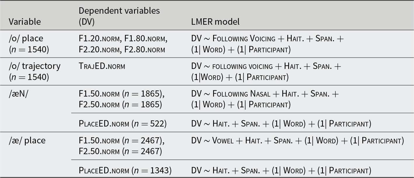
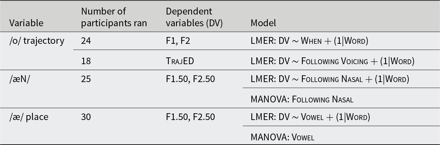
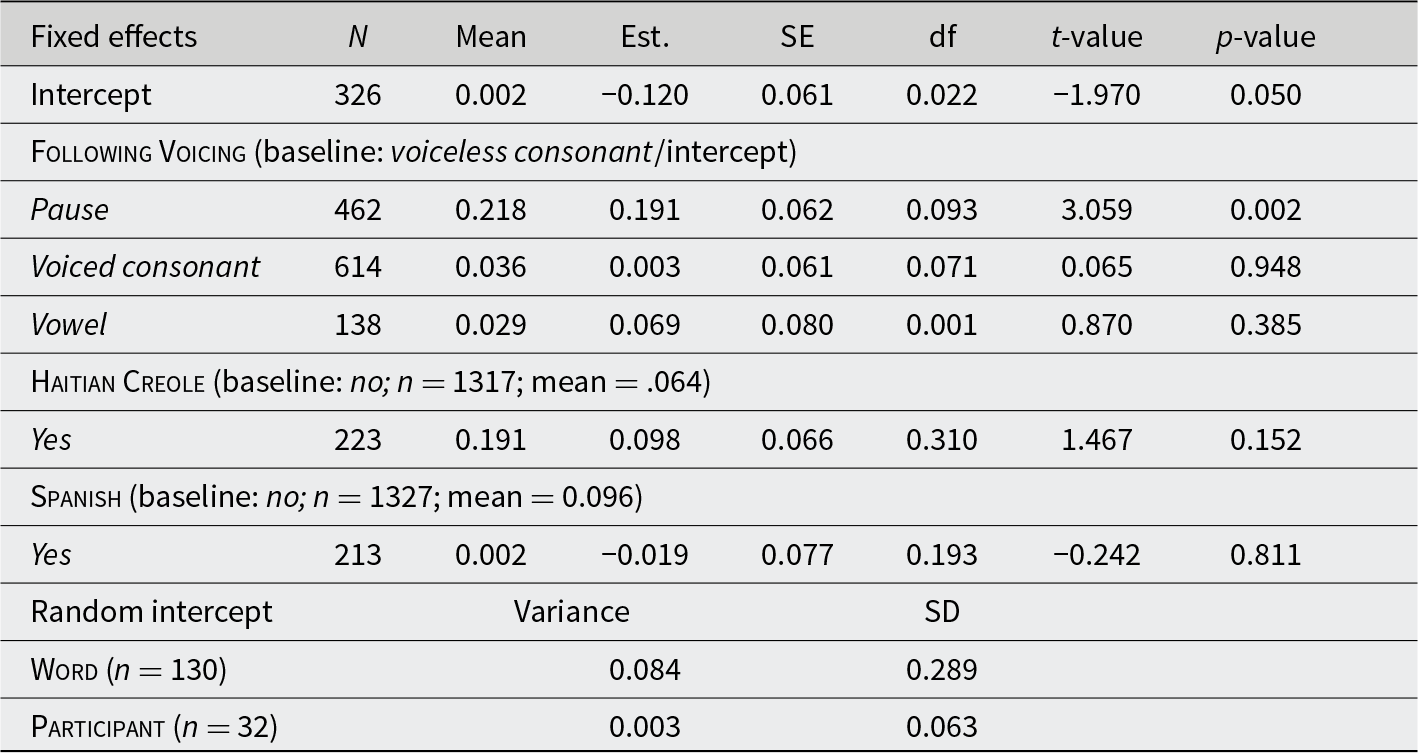
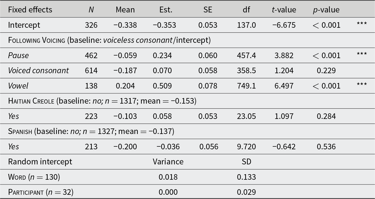
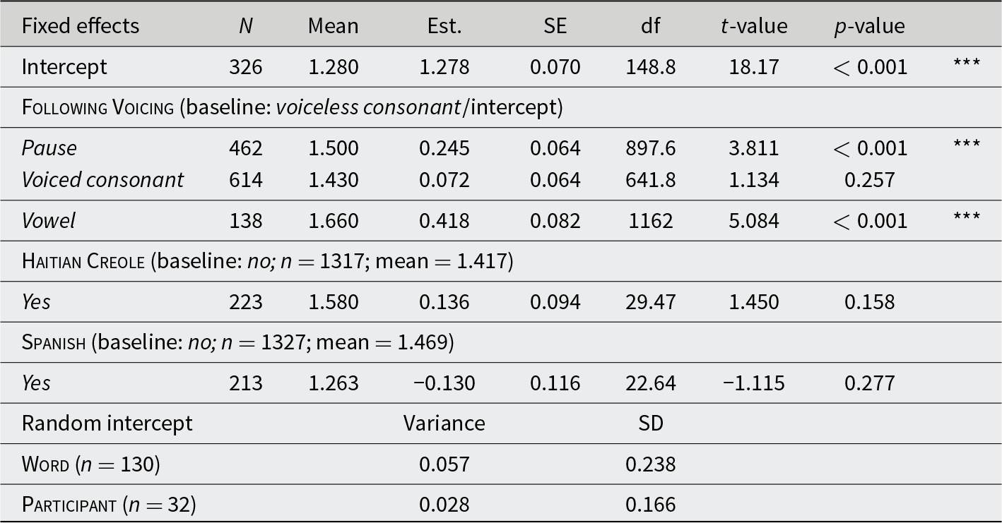
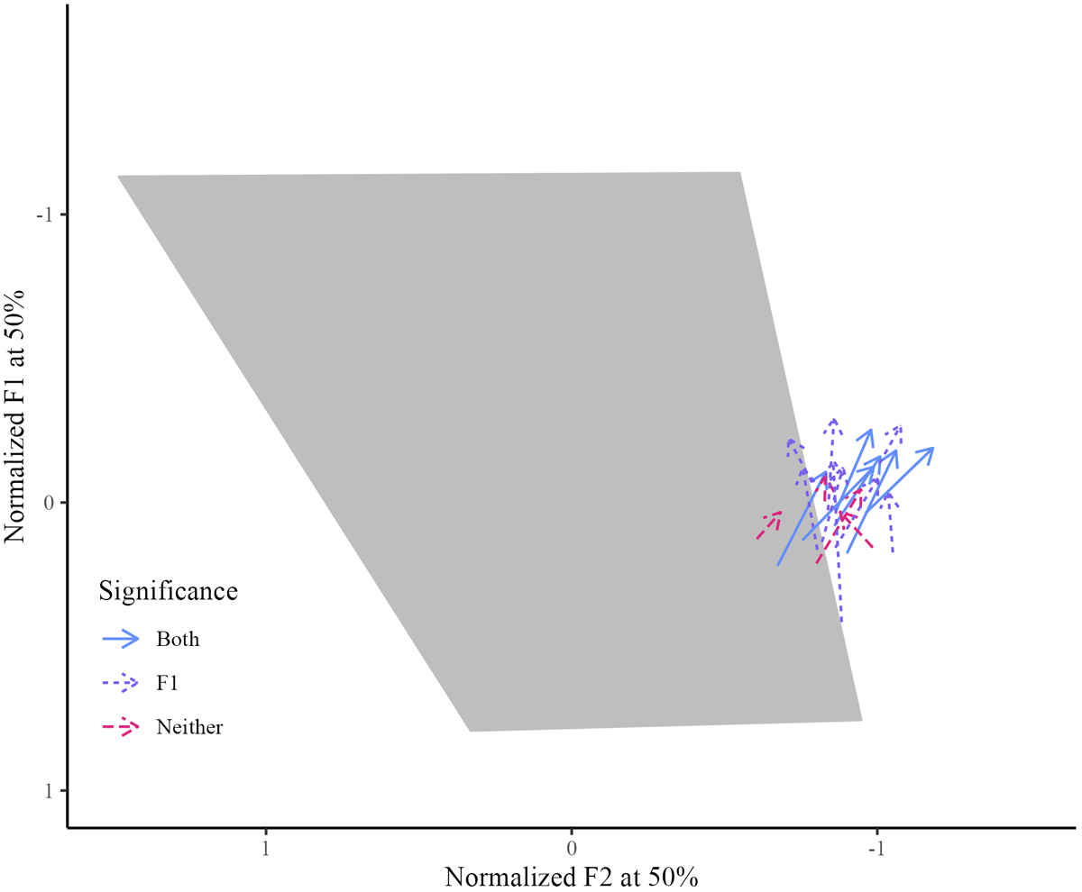
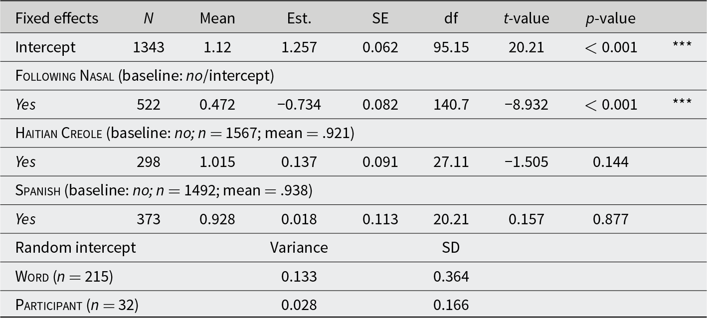
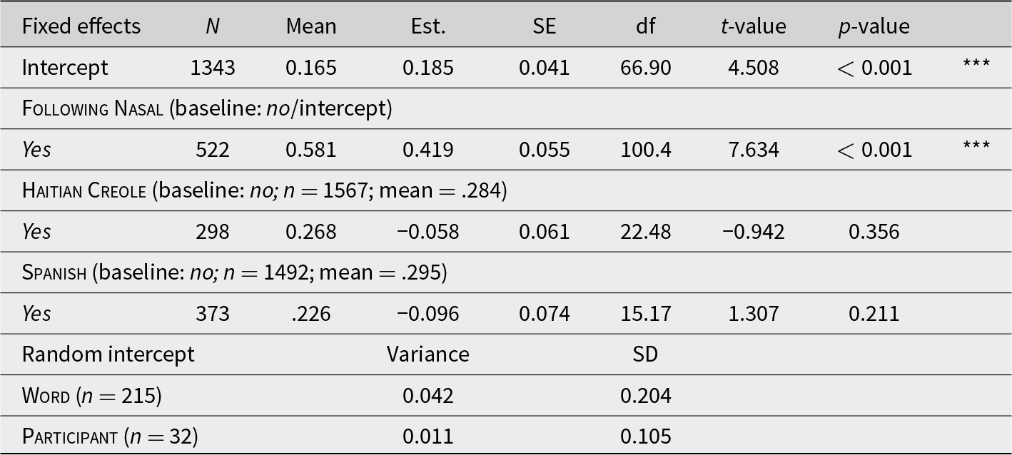
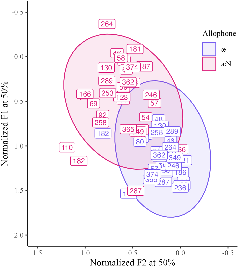
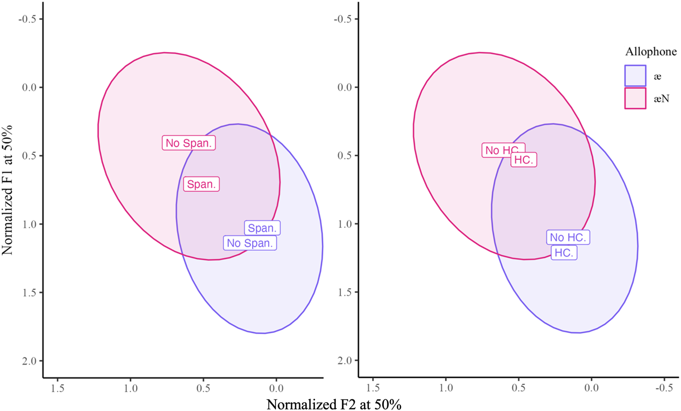
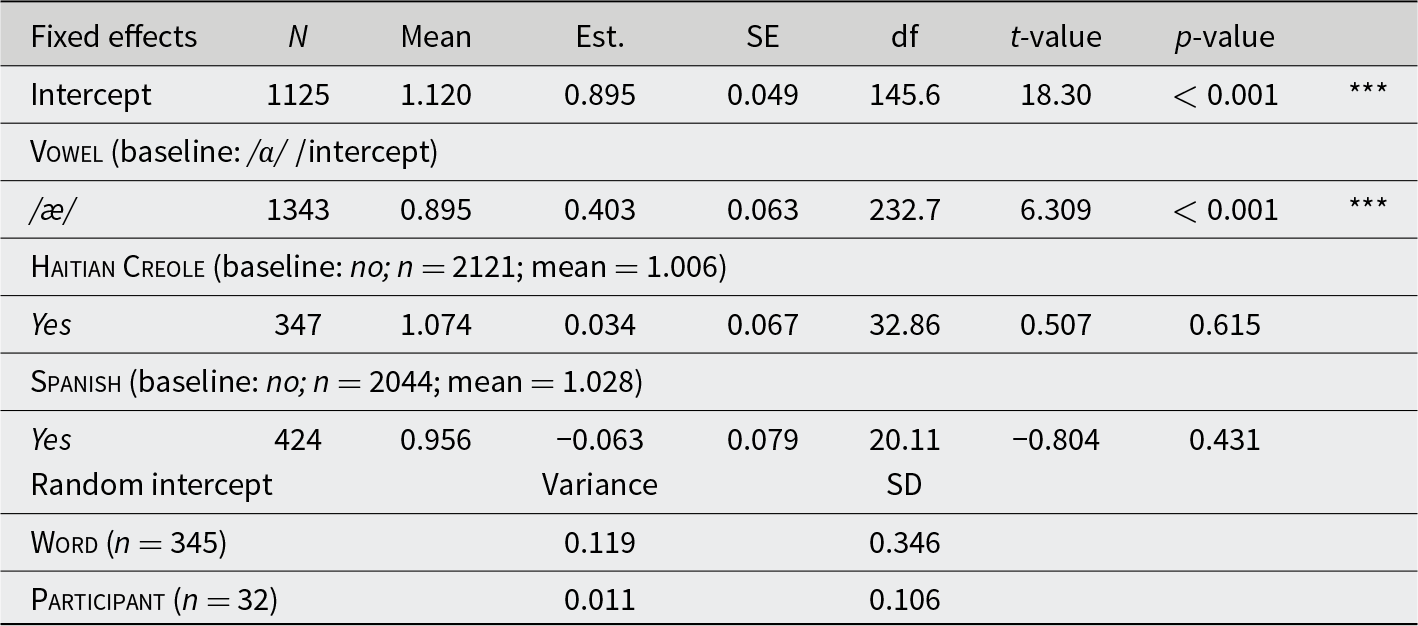
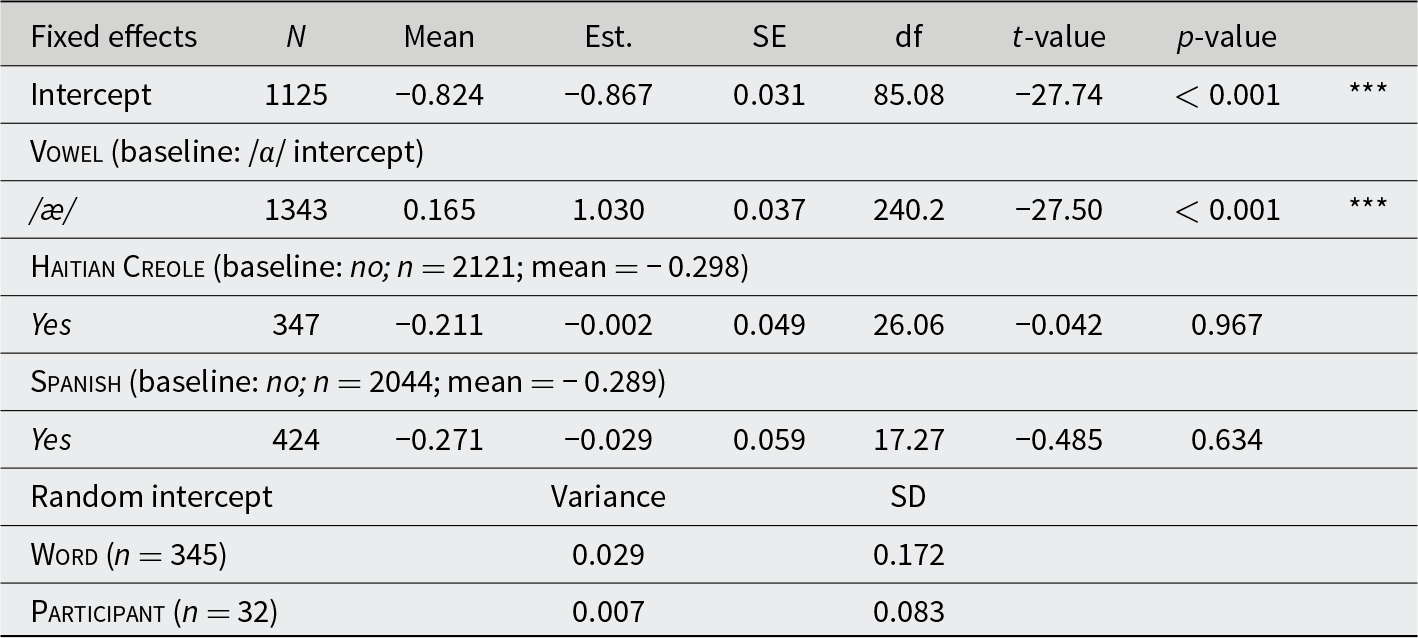
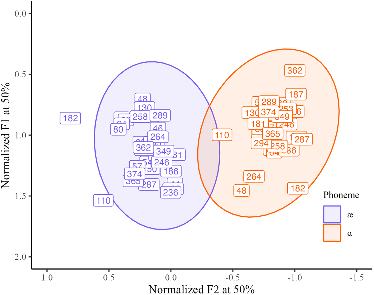
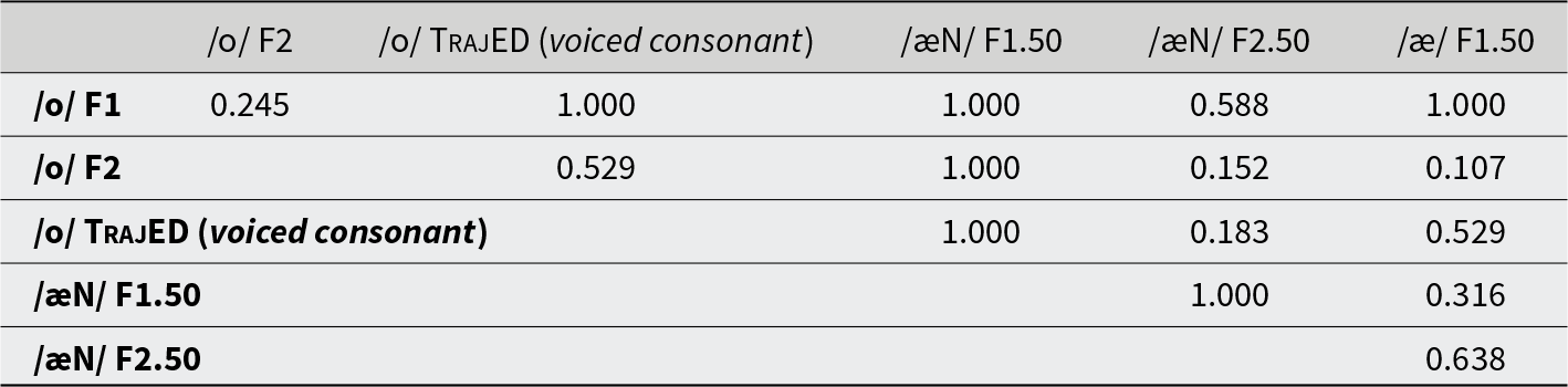
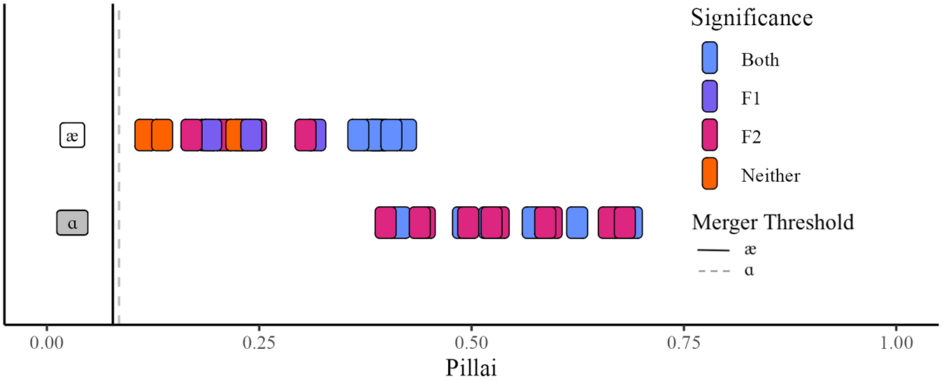
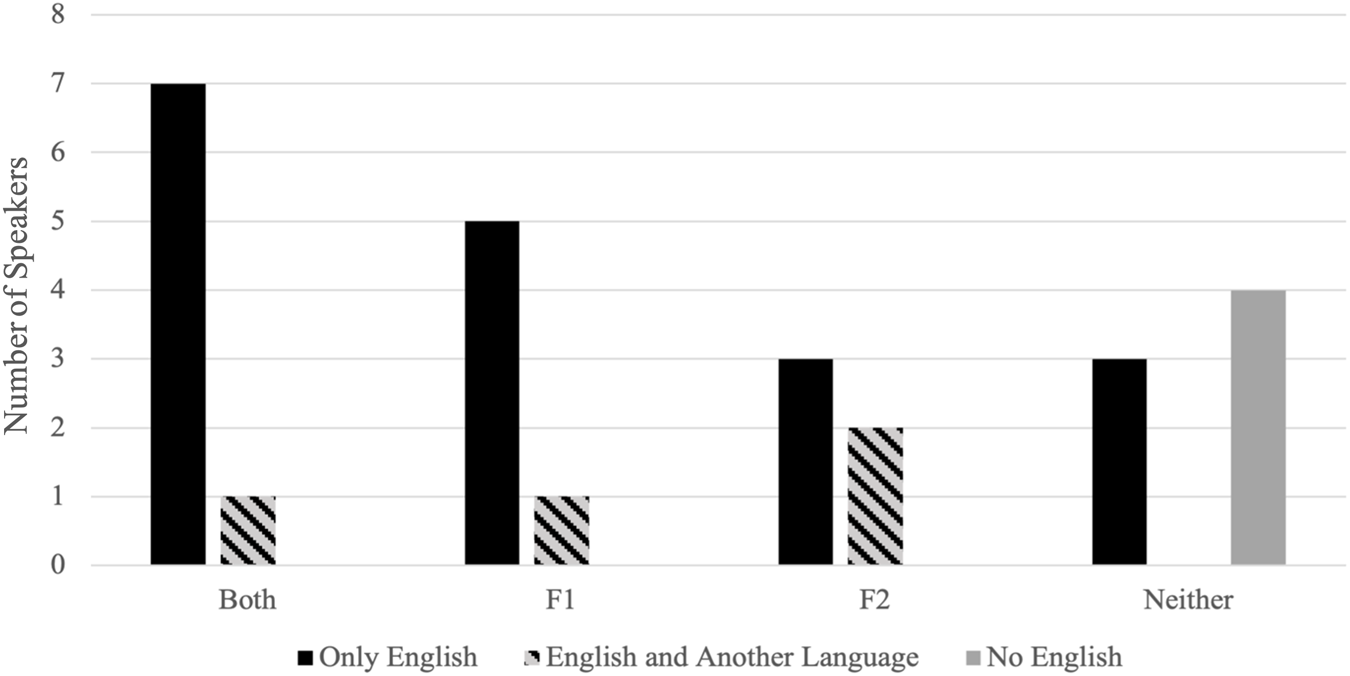
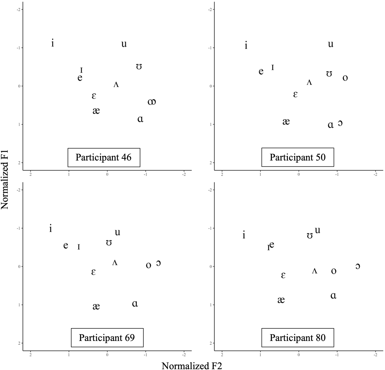
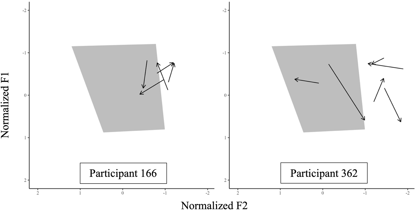
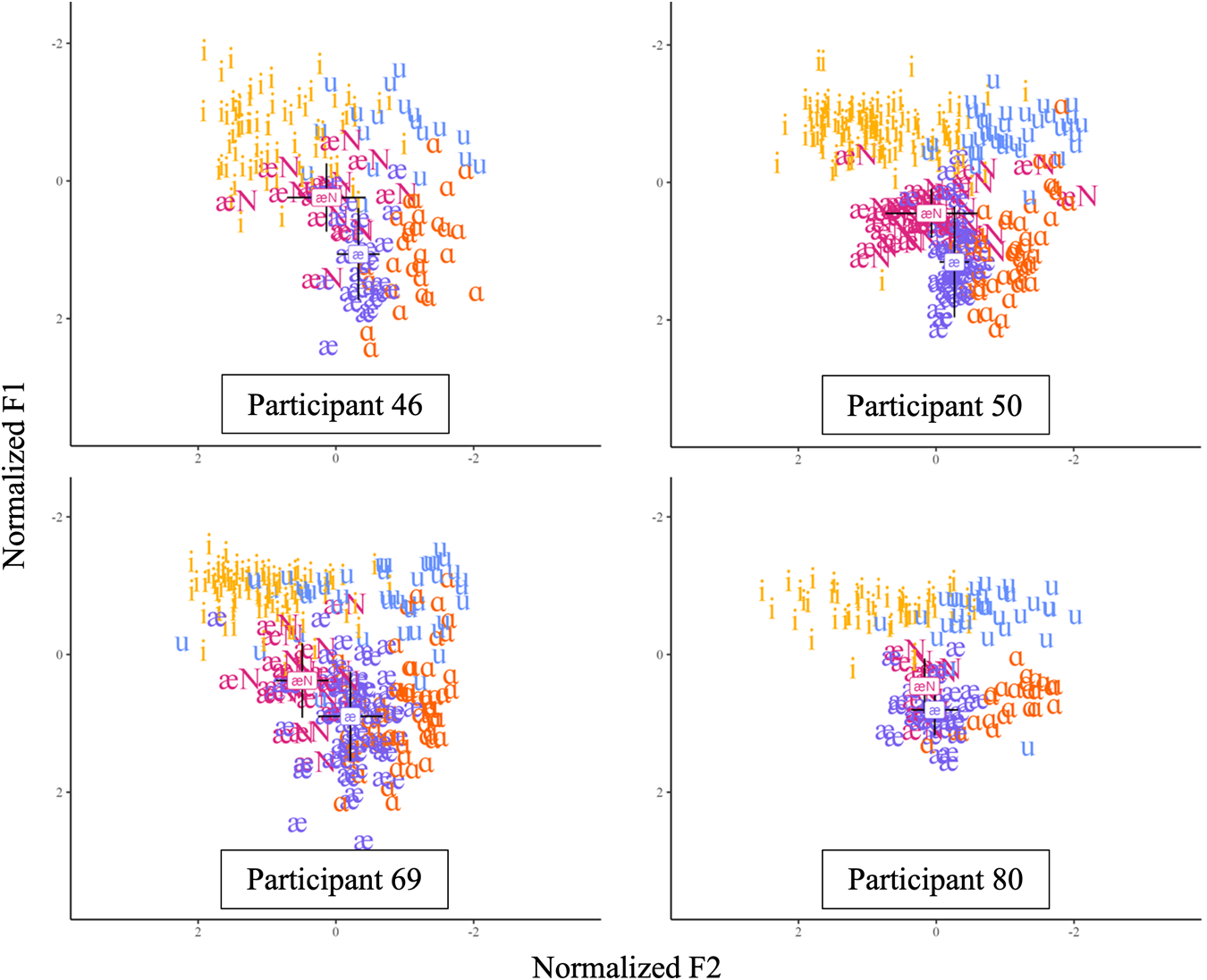
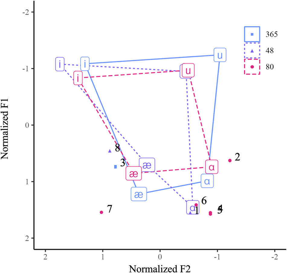

 Open access

