





1. Introduction
Investigating the propagation of acoustic and entropy fluctuations through nozzles with area variations is of interest for a wide variety of engineering applications, particularly those involving combustion noise and thermoacoustic instabilities. The propagation of acoustic and entropy waves towards the outlet generates direct and indirect noise, respectively (Marble & Candel Reference Marble and Candel1977; Dowling & Mahmoudi Reference Dowling and Mahmoudi2015; Morgans & Duran Reference Morgans and Duran2016; Ihme Reference Ihme2017). Direct noise arises from acoustic fluctuations within the combustion chamber that propagate through the turbine stages, whereas indirect noise is produced when entropy, vorticity or compositional waves are accelerated through the turbine (Howe Reference Howe2003; Morgans & Duran Reference Morgans and Duran2016; Magri Reference Magri2017). When studying thermoacoustic instabilities in combustion chambers, the propagation of acoustic and entropy waves through the chamber’s inlet and outlet plays a crucial role, as it strongly influences the acoustic impedances perceived upstream and downstream (Leyko, Nicoud & Poinsot Reference Leyko, Nicoud and Poinsot2009; Goh & Morgans Reference Goh and Morgans2013; Morgans & Yang Reference Morgans and Yang2025).
The propagation of waves through nozzles was first studied by Tsien (Reference Tsien1952), who analysed the propagation of acoustic waves through a quasi-one-dimensional nozzle with a spatially linear velocity profile. Marble & Candel (Reference Marble and Candel1977) formulated an analytical solution for the transfer function applicable to both subcritical and supercritical nozzle flows, where subcritical and supercritical refer to flows that remain entirely subsonic throughout the nozzle and to flows that become choked and accelerate to supersonic conditions downstream of the throat, respectively. This solution remains applicable in the compact (or zero-frequency) limit, assuming that the acoustic and entropy wavelengths substantially exceed the length scale over which changes in nozzle area occur. Subsequently, Stow, Dowling & Hynes (2002) and Goh & Morgans (Reference Goh and Morgans2011) extended this compact solution to non-zero frequencies using an asymptotic expansion of the linearised Euler equations with respect to frequency. Several experimental and numerical studies have since confirmed the generation of both direct and indirect noise in nozzle and blade-acceleration configurations, providing further validation of these theoretical models (Cumpsty & Marble Reference Cumpsty and Marble1977; Bake et al. Reference Bake, Richter, Mühlbauer, Kings, Röhle, Thiele and Noll2009; Leyko et al. Reference Leyko, Nicoud and Poinsot2009; Giusti et al. Reference Giusti, Worth, Mastorakos and Dowling2017; Guzmán-Iñigo et al. Reference Guzmán-Iñigo, Durán and Morgans2021).
Following the assumptions established by Marble & Candel (Reference Marble and Candel1977) – namely, inviscid, isentropic and quasi-one-dimensional flow – Duran & Moreau (Reference Duran and Moreau2013) introduced a solution valid across all frequencies using the Magnus-expansion method, which was well developed by Blanes et al. (Reference Blanes, Casas, Oteo and Ros2009). Duran & Morgans (Reference Duran and Morgans2015) later extended the Magnus-expansion method to a two-dimensional annular configuration including circumferential waves. Magri (Reference Magri2017) employed the Dyson expansion-based method to solve for the acoustic field sustained in a nozzle with incoming compositional inhomogeneities where the mean flow was assumed to be isentropic. Younes & Hickey (Reference Younes and Hickey2019) combined the compound flow equation with the Magnus-expansion method to model the acoustic response in a compound-compressible nozzle. Olivon et al. (Reference Olivon, Genot, Hirschberg, Moreau and Hirschberg2025) developed a new generalised boundary condition for the choked-nozzle throat to ensure regularity and improve the consistency of acoustic response predictions. These contributions are embedded within the wider effort of modelling indirect combustion noise (Ihme Reference Ihme2017), which becomes especially important at low frequencies and in high-Mach-number conditions.
These investigations, however, are limited to isentropic mean flows and are therefore not applicable to cases involving flow non-isentropicity. In practice, many nozzle flows are non-isentropic due to effects such as wall friction, heat transfer or flow separation. In particular, viscous wall friction is unavoidable in realistic nozzle configurations and can significantly modify the mean-flow distribution as well as the propagation and coupling of acoustic and entropy waves. Recent studies by De Domenico et al. (Reference De, Francesca, Erwan, Rodrigues, Magri and Hochgreb2021) and Yang, Guzmán-Iñigo & Morgans (Reference Yang, Guzmán-Iñigo and Morgans2020) have shown that flow separation in the diverging section of realistic nozzles can lead to recirculation zones, increased turbulence and deviations from isentropic behaviour, all of which significantly influence acoustic transmission. Huet, Emmanuelli & Ducruix (Reference Huet, Emmanuelli and Ducruix2021) assessed the role of viscosity in entropy noise generation within a nozzle through analytical modelling and numerical simulations, and reported that noise generation and scattering are slightly reduced in the medium-frequency range. Furthermore, Yeddula, Gaudron & Morgans (Reference Yeddula, Gaudron and Morgans2021) demonstrated that steady heat transfer can substantially alter nozzle acoustics. A Magnus-expansion-based model for predicting the transfer functions of nozzle flows with steady heat transfer was subsequently proposed by Yeddula, Guzmán-Iñigo & Morgans (Reference Yeddula, Guzmán-Iñigo and Morgans2022). In parallel, Jain & Magri (Reference Jain and Magri2022) numerically investigated a convergent–divergent nozzle with dissipation and reported significant effects on the gain and phase of the reflected and transmitted waves. More recently, Char et al. (Reference Char, Giraudi, Newman and Morgans2025) developed an analytical model for the acoustic field in non-adiabatic milli-scale flows with axial temperature gradients and visco-thermal losses, based on an inviscid formulation with wavenumber corrections, which provides accurate predictions at high frequencies.
In this paper, we present a general analytical framework for acoustic and entropy waves propagating through a quasi-one-dimensional nozzle, in which wall friction is incorporated directly into the governing equations as a source of flow non-isentropicity. The newly proposed linearised Euler formulation retains both the steady and unsteady contributions of wall friction, leading to a new perturbation system that captures the coupling between wall friction, entropy fluctuations and acoustic waves. Building on the Magnus-expansion method proposed by Duran & Moreau (Reference Duran and Moreau2013), the resulting wall-friction formulation is solved analytically for arbitrary frequencies within the quasi-one-dimensional framework. The solution applies to both subcritical and supercritical flow regimes in the presence of wall friction. The formulation is further extended to include steady heat transfer, allowing the combined effects of wall friction and heat transfer to be treated consistently within the same analytical framework. Previous analytical nozzle-acoustics formulations have mostly assumed isentropic mean flows or have represented dissipative effects in simplified forms. Although Yeddula et al. (Reference Yeddula, Guzmán-Iñigo and Morgans2022) extended the frequency-resolved analytical framework to include steady heat transfer, wall friction has so far not been incorporated directly into the quasi-one-dimensional linearised Euler equations in a consistent analytical and frequency-resolved manner. To the best of our knowledge, the present work is the first to incorporate wall friction and heat transfer directly into this formulation and to treat the resulting non-isentropic source terms consistently, thereby enabling the modelling of non-isentropic nozzle flows over a wide range of frequencies and Mach numbers.
This paper presents the mathematical model with a physical interpretation of the equations for the nozzle flow with wall friction in § 2 followed by the implementation of an analytical method to solve the differential equations via the Magnus expansion in § 3. Results and validations applied to a converging–diverging nozzle with wall friction are illustrated in § 4, and the solution considering both wall friction and steady heat transfer is then derived and validated further in § 5. Conclusions are drawn in § 6.
2. Non-isentropic linearised Euler equations with wall friction
The nozzle with varying area and wall friction is shown in figure 1. The gas inside the nozzle is assumed to be an ideal, calorically perfect gas, and the flow is considered inviscid and compressible. The present analysis adopts a quasi-one-dimensional formulation, in which the nozzle is assumed to be sufficiently long compared with its characteristic transverse dimension, such that the mean flow varies predominantly in the axial direction. In this framework, the flow variables at each axial location are taken as cross-sectional averages. In addition, the wavelengths of the acoustic and entropy perturbations of interest are assumed to be large compared with the transverse length scale of the nozzle, so that transverse variations of the perturbation fields remain weak (Duran & Moreau Reference Duran and Moreau2013).
Sketch of the acoustic and entropy waves in a converging–diverging nozzle with skin friction factor, $f$
, along all nozzle walls.
$f$
, along all nozzle walls.

Although the effects of wall friction are, in essence, not strictly one-dimensional, they are incorporated here through an equivalent axial momentum loss within the quasi-one-dimensional framework for modelling purposes. The Fanning friction factor $f(x)$
, which can vary axially along the nozzle, is used to express the wall-friction effects. Here, the volumetric forces, mass diffusion and heat transfer are not taken into account, and the continuity and momentum equations can be given as
$f(x)$
, which can vary axially along the nozzle, is used to express the wall-friction effects. Here, the volumetric forces, mass diffusion and heat transfer are not taken into account, and the continuity and momentum equations can be given as
 \begin{align} A\frac {{\partial \rho }}{{\partial t}} + \frac {{\partial (\rho Au)}}{{\partial x}} &= 0, \end{align}
 \begin{align} \frac {{\partial u}}{{\partial t}} + u\frac {{\partial u}}{{\partial x}} + \frac {1}{\rho }\frac {{\partial p}}{{\partial x}} &= - \frac {{4f}}{D}\frac {{{u^2}}}{2}, \end{align}
where $u$
,
$u$
, $\rho$
and
$\rho$
and $p$
denote the flow axial velocity, density and pressure, respectively. Here, the Fanning friction factor
$p$
denote the flow axial velocity, density and pressure, respectively. Here, the Fanning friction factor $f$
is defined via the wall shear stress
$f$
is defined via the wall shear stress $\tau _w=f\rho u^2/2$
, and is equal to one fourth the Darcy–Weisbach friction factor. Also,
$\tau _w=f\rho u^2/2$
, and is equal to one fourth the Darcy–Weisbach friction factor. Also, $A$
stands for the cross-sectional area of the nozzle, and
$A$
stands for the cross-sectional area of the nozzle, and $D$
denotes the diameter of the nozzle. Equation (2.2) represents the quasi-one-dimensional momentum equation for compressible flow with wall friction. It is obtained by applying an axial momentum balance to a control volume of variable cross-sectional area under the quasi-one-dimensional approximation, in which transverse velocity components are neglected. The effect of wall friction enters through the streamwise wall shear stress, resulting in a momentum loss term proportional to the friction factor and the wetted perimeter. Related derivations and formulations of the quasi-one-dimensional momentum equation with friction can be found in classical treatments of compressible internal flows (Shapiro Reference Shapiro1953).
$D$
denotes the diameter of the nozzle. Equation (2.2) represents the quasi-one-dimensional momentum equation for compressible flow with wall friction. It is obtained by applying an axial momentum balance to a control volume of variable cross-sectional area under the quasi-one-dimensional approximation, in which transverse velocity components are neglected. The effect of wall friction enters through the streamwise wall shear stress, resulting in a momentum loss term proportional to the friction factor and the wetted perimeter. Related derivations and formulations of the quasi-one-dimensional momentum equation with friction can be found in classical treatments of compressible internal flows (Shapiro Reference Shapiro1953).
Following the first law of thermodynamics, the conservation of energy for adiabatic nozzle flow with varying area and wall friction can be given as
 \begin{equation} \frac {{\partial \left ( {\rho {e_t}A\text{d}x} \right )}}{{\partial t}} + \frac {{\partial \left ( {\rho {e_t}uA} \right )}}{{\partial x}}\text{d}x + \frac {{\partial \left ( {puA} \right )}}{{\partial x}}\text{d}x = 0\, ,\end{equation}
with $e_t=e+u^2/2$
standing for the total energy per unit mass. Expanding the equation and subtracting the mass continuity (2.1) from it, we obtain
$e_t=e+u^2/2$
standing for the total energy per unit mass. Expanding the equation and subtracting the mass continuity (2.1) from it, we obtain
 \begin{equation} \rho \frac {{\text{D}e}}{{\text{D}t}} + \frac {\rho }{2}\frac {{\text{D}{u^2}}}{{\text{D}t}} + \frac {1}{A}\frac {{\partial \left ( {puA} \right )}}{{\partial x}} = 0\ ,\end{equation}
where $e$
is the internal energy per unit and
$e$
is the internal energy per unit and $D/Dt=(\partial /\partial t)+u(\partial /\partial x)$
represents the total derivative. The entropy change can be evaluated from the thermodynamic relationship
$D/Dt=(\partial /\partial t)+u(\partial /\partial x)$
represents the total derivative. The entropy change can be evaluated from the thermodynamic relationship
 \begin{equation} T\text{d}s = \text{d}e - \big ( {p/{\rho ^2}} \big )\text{d}\rho ,\end{equation}
where $T$
and
$T$
and $s$
represent the temperature and entropy, respectively. Substituting the above equation and momentum (2.2) into (2.4) yields the energy conservation equation expressed in terms of entropy. It reads
$s$
represent the temperature and entropy, respectively. Substituting the above equation and momentum (2.2) into (2.4) yields the energy conservation equation expressed in terms of entropy. It reads
 \begin{equation} \frac {{\partial s}}{{\partial t}} + u\frac {{\partial s}}{{\partial x}} = \frac {{4f}}{D}\frac {{{u^3}}}{2}\frac {{\rho R}}{p}\quad ,\end{equation}
where $R$
is the gas constant. Equation (2.6) is derived directly from the unsteady energy conservation with wall friction, in contrast to the formulation given by Jain & Magri (Reference Jain and Magri2022), which relates entropy generation to total-pressure loss and then evaluates the total-pressure change from the steady frictional flow. In the present work, the effect of wall friction is incorporated explicitly and consistently at the level of the unsteady governing equations, which is essential for linearisation and for capturing the unsteady contribution of wall friction to nozzle acoustics.
$R$
is the gas constant. Equation (2.6) is derived directly from the unsteady energy conservation with wall friction, in contrast to the formulation given by Jain & Magri (Reference Jain and Magri2022), which relates entropy generation to total-pressure loss and then evaluates the total-pressure change from the steady frictional flow. In the present work, the effect of wall friction is incorporated explicitly and consistently at the level of the unsteady governing equations, which is essential for linearisation and for capturing the unsteady contribution of wall friction to nozzle acoustics.
Together with the state equation $p=\rho RT$
, (2.1), (2.2) and (2.6) form the governing equations for quasi-one-dimensional nozzle flow with wall friction.
$p=\rho RT$
, (2.1), (2.2) and (2.6) form the governing equations for quasi-one-dimensional nozzle flow with wall friction.
Under the linearisation assumption, the thermodynamic and flow variables are decomposed into a steady, time-averaged mean component and a time-dependent fluctuating component, which are denoted by an overbar and a prime, respectively. This decomposition enables the analysis of unsteady, small-amplitude perturbations superimposed on a steady base flow. The governing equations are then linearised with respect to these variables, and the mean components are collected and balanced, yielding the following system:
 \begin{align} &\frac {1}{{\bar \rho }}\frac {{{\textrm {d}}\bar \rho }}{{{\textrm {d}}x}} + \frac {1}{{\bar u}}\frac {{{\textrm {d}}\bar u}}{{{\textrm {d}}x}} + \frac {1}{A}\frac {{{\textrm {d}}A}}{{{\textrm {d}}x}} = 0, \end{align}
 \begin{align} &\ \, \bar u\frac {{{\textrm {d}}\bar u}}{{{\textrm {d}}x}} + \frac {1}{{\bar \rho }}\frac {{{\textrm {d}}\bar p}}{{{\textrm {d}}x}} = - \frac {{4f}}{D}\frac {{{{\bar u}^2}}}{2}, \end{align}
 \begin{align} &\quad \ \bar u\frac {{{\textrm {d}}\bar s}}{{{\textrm {d}}x}} = \frac {{4f}}{D}\frac {{{{\bar u}^3}}}{2}\frac {{\bar \rho R}}{{\bar p}}, \end{align}
 \begin{align} &\qquad \bar p = \bar \rho R\bar T. \end{align}
Here, we normalise the time-dependent quantities as
 \begin{equation} \hat p = {{p'}}/({{\gamma \bar p}}), \hat u = {{u'}}/{{\bar u}}, \hat s = {{s'}}/{{{c_p}}} ,\end{equation}
with $c_p$
denoting the specific heat capacity at constant pressure. By subtracting the mean components from the governing equations and retaining only the first-order fluctuating terms, the quasi-one-dimensional linearised Euler equations (LEE) for nozzle flow with wall friction are obtained in dimensionless form as
$c_p$
denoting the specific heat capacity at constant pressure. By subtracting the mean components from the governing equations and retaining only the first-order fluctuating terms, the quasi-one-dimensional linearised Euler equations (LEE) for nozzle flow with wall friction are obtained in dimensionless form as
 \begin{align}&\quad \frac {{\partial \hat p}}{{\partial t}} + \bar u\frac {{\partial \left ( {\hat p + \hat u} \right )}}{{\partial x}} = \frac {{\gamma - 1}}{\gamma }\frac {{\bar \rho }}{{\bar p}}\frac {{4f}}{D}\frac {{{{\bar u}^3}}}{2}\left ( {2\hat u - \left ( {\gamma - 1} \right )\hat p - \hat s} \right )\!, \end{align}
 \begin{align}& \frac {{\partial \hat u}}{{\partial t}} + \bar u\frac {{\partial \hat u}}{{\partial x}} + \frac {{{{\bar c}^2}}}{{\bar u}}\frac {{\partial \hat p}}{{\partial x}} + \left ( {\frac {{\partial \bar u}}{{\partial x}} + \frac {{4f}}{D}\frac {{\bar u}}{2}} \right )\left ( {2\hat u - \left ( {\gamma - 1} \right )\hat p - \hat s} \right ) = 0, \end{align}
 \begin{align}&\qquad\,\, \frac {{\partial \hat s}}{{\partial t}} + \bar u\frac {{\partial \hat s}}{{\partial x}} = \frac {{\gamma - 1}}{\gamma }\frac {{\bar \rho }}{{\bar p}}\frac {{4f}}{D}\frac {{{{\bar u}^3}}}{2}\left ( {2\hat u - \left ( {\gamma - 1} \right )\hat p - \hat s} \right )\!, \end{align}
where $\bar c$
and
$\bar c$
and $\gamma$
stand for the mean adiabatic speed of sound and the adiabatic index or heat capacity ratio, respectively. Equations (2.12)–(2.14) form a self-consistent set of linearised governing equations for non-isentropic nozzle flows with wall friction. They show that wall friction influences the unsteady dynamics through two complementary mechanisms: indirectly via the modified mean flow, and directly through source terms proportional to the friction factor that appear explicitly in the linearised equations. These source terms appear not only in the momentum equation, but also in the pressure and entropy equations, yielding a fully coupled description of acoustic, velocity and entropy fluctuations in the presence of friction.
$\gamma$
stand for the mean adiabatic speed of sound and the adiabatic index or heat capacity ratio, respectively. Equations (2.12)–(2.14) form a self-consistent set of linearised governing equations for non-isentropic nozzle flows with wall friction. They show that wall friction influences the unsteady dynamics through two complementary mechanisms: indirectly via the modified mean flow, and directly through source terms proportional to the friction factor that appear explicitly in the linearised equations. These source terms appear not only in the momentum equation, but also in the pressure and entropy equations, yielding a fully coupled description of acoustic, velocity and entropy fluctuations in the presence of friction.
To obtain the wave transfer functions using a Magnus-expansion approach, the normalised mass flow rate, total temperature and entropy fluctuations that are invariants of the isentropic flow at zero frequency are chosen as the variables for recasting the LEE. They read
 \begin{equation} {I_A} = {\dot m}'/{\bar {\dot m}}, {I_B} = {T_t}^\prime /{{\bar T}_t}, {I_c} = s'/{c_p}. \end{equation}
These invariants can be expressed in terms of the dimensionless primitive variables $\hat p$
,
$\hat p$
, $\hat u$
and
$\hat u$
and $\hat s$
as follows:
$\hat s$
as follows:
 \begin{align} {I_A} &= \hat u + \hat p - \hat s, \end{align}
 \begin{align} {I_B} &= \left ( {\gamma - 1} \right )\frac {{{M^2}\hat u + \hat p + \hat s/\left ( {\gamma - 1} \right )}}{{1 + \left ( {\gamma - 1} \right ){M^2}/2}}, \end{align}
 \begin{align} {I_C} &= \hat s , \end{align}
with $M={\bar u}/{\bar c}$
denoting the mean local Mach number. Given a vector containing the above invariants
$M={\bar u}/{\bar c}$
denoting the mean local Mach number. Given a vector containing the above invariants $\boldsymbol{I} =[I_A\ I_B\ I_C]^T$
, the LEE can be recast in the matrix form as
$\boldsymbol{I} =[I_A\ I_B\ I_C]^T$
, the LEE can be recast in the matrix form as
 \begin{equation} \frac {\partial }{{\partial t}}{\boldsymbol{{ I}}} + \bar u{{\boldsymbol{E}}_{{x}}}\frac {\partial }{{\partial x}}{\boldsymbol{I}} + \frac {{4f}}{D}\frac {{\bar u}}{2}{{\boldsymbol{E}}_{{s}}}{\boldsymbol{I}} = 0, \end{equation}
where ${\boldsymbol{E}}_{{x}}$
and
${\boldsymbol{E}}_{{x}}$
and ${\boldsymbol{E}}_{{s}}$
are non-constant 3
${\boldsymbol{E}}_{{s}}$
are non-constant 3 $\times$
3 matrices defined by the mean flow. They read
$\times$
3 matrices defined by the mean flow. They read
 \begin{equation} {{\boldsymbol{E}}_{{x}}} = \left [ {\begin{array}{*{20}{c}} 1&{\frac {\varLambda }{{\left ( {\gamma - 1} \right ){M^2}}}}&{ - \frac {1}{{\left ( {\gamma - 1} \right ){M^2}}}}\\[8pt] {\frac {{\gamma - 1}}{\varLambda }}&1&{\frac {{\gamma - 1}}{\varLambda }}\\[8pt] 0&0&1 \end{array}} \right ]\!, \end{equation}
 \begin{align} & {{\boldsymbol{E}}_{{s}}} = \dfrac {1}{{{M^2} - 1}} \nonumber \\ &\quad \times\left [\!\!\! {\begin{array}{*{20}{c}} { - 2\varLambda }&{\dfrac {{\varLambda \left ( {\gamma + 1} \right )}}{{\left ( {\gamma - 1} \right )}}}&{ - \dfrac {1}{{\left ( {\gamma - 1} \right ){M^2}}}}\\[12pt] { - 2\left ( {\gamma - 1} \right )\!\left ( \!{{M^2} - \dfrac {{\bar \rho }}{{\bar p}}{{\bar u}^2}} \right )}&{\left ( \!{{M^2} - \dfrac {{\bar \rho }}{{\bar p}}{{\bar u}^2}} \right )\!\left ( {\gamma + 1} \right )}&{\dfrac {{\gamma - 1}}{\varLambda }\!\left (\! {{M^2} - \dfrac {{\bar \rho }}{{\bar p}}{{\bar u}^2}} \right )\!\left (\! { - \gamma {M^2} - \dfrac {{2\gamma }}{{\gamma - 1}}} \right )}\\[12pt] {2\varLambda \dfrac {{\gamma - 1}}{\gamma }\dfrac {{\bar \rho }}{{\bar p}}{{\bar u}^2}}&{ - \varLambda \dfrac {{\gamma + 1}}{\gamma }\dfrac {{\bar \rho }}{{\bar p}}{{\bar u}^2}}&{ - \dfrac {{\gamma - 1}}{\gamma }\dfrac {{\bar \rho }}{{\bar p}}{{\bar u}^2}\left ( { - \gamma {M^2} - \dfrac {{2\gamma }}{{\gamma - 1}}} \right )} \end{array}} \!\!\!\!\right ]\!, \end{align}
where $\varLambda =1+(\gamma -1)M^2/2$
.
$\varLambda =1+(\gamma -1)M^2/2$
.
3. General analytical solution
Assuming the above time-dependent fluctuating quantities to be harmonic, we can take $\hat z=z^*e^{i\omega t}$
, where
$\hat z=z^*e^{i\omega t}$
, where $\omega$
stands for the angular frequency and
$\omega$
stands for the angular frequency and $z^*$
is the wave amplitude. Applying the temporal Fourier transform to recast (2.19) in the frequency domain yields
$z^*$
is the wave amplitude. Applying the temporal Fourier transform to recast (2.19) in the frequency domain yields
 \begin{equation} \begin{array}{*{20}{c}} {\frac {\text{d}}{{\text{d}x}}{\boldsymbol{I}} = {\boldsymbol{A}}(x,\omega ,f){\boldsymbol{I}}},& \text{where} \quad {{\boldsymbol{A}} = - {{[{{\boldsymbol{E}}_{{x}}}]}^{ - 1}}\left ( {\frac {{i\omega }}{{\bar u}}{\boldsymbol{J}} + \frac {{4f}}{{2D}}{{\boldsymbol{E}}_{{s}}}} \right )}, \end{array} \end{equation}
with $\boldsymbol{J}$
denoting a third-order identity matrix. Equation (3.1) is similar to the equation obtained by Duran & Moreau (Reference Duran and Moreau2013) but with an extra term, involving the matrix
$\boldsymbol{J}$
denoting a third-order identity matrix. Equation (3.1) is similar to the equation obtained by Duran & Moreau (Reference Duran and Moreau2013) but with an extra term, involving the matrix $E_s$
, which accounts for wall-friction effects. The above formulation requires the matrix
$E_s$
, which accounts for wall-friction effects. The above formulation requires the matrix ${\boldsymbol{E}}_{{x}}$
to be invertible. When the determinant of
${\boldsymbol{E}}_{{x}}$
to be invertible. When the determinant of ${\boldsymbol{E}}_{{x}}$
is non-zero, i.e.
${\boldsymbol{E}}_{{x}}$
is non-zero, i.e. $M \ne 1$
, the matrix
$M \ne 1$
, the matrix $\boldsymbol{A}$
is well defined. For choked-nozzle flows, the Mach number reaches unity at the throat, where
$\boldsymbol{A}$
is well defined. For choked-nozzle flows, the Mach number reaches unity at the throat, where $\det ({\boldsymbol{E}}_{{x}})=0$
and the matrix system cannot be inverted. This case will be discussed in § 3.2.
$\det ({\boldsymbol{E}}_{{x}})=0$
and the matrix system cannot be inverted. This case will be discussed in § 3.2.
The position and frequency are specified in terms of the non-dimensional parameters $\xi =x/L$
(dimensionless axial coordinate) and
$\xi =x/L$
(dimensionless axial coordinate) and $\textit{He} = \omega L/\bar c_0$
(axial Helmholtz number), respectively, where
$\textit{He} = \omega L/\bar c_0$
(axial Helmholtz number), respectively, where $L$
denotes the nozzle length and
$L$
denotes the nozzle length and $\bar c_0$
corresponds to the stagnation speed of sound at the inlet. The first-order system of differential (3.1) is solved using a Magnus-expansion-based method (Blanes et al. Reference Blanes, Casas, Oteo and Ros2009). In this method, the solution is expressed as an infinite expansion around the axial Helmholtz number
$\bar c_0$
corresponds to the stagnation speed of sound at the inlet. The first-order system of differential (3.1) is solved using a Magnus-expansion-based method (Blanes et al. Reference Blanes, Casas, Oteo and Ros2009). In this method, the solution is expressed as an infinite expansion around the axial Helmholtz number $\textit{He}$
and the wall-friction factor
$\textit{He}$
and the wall-friction factor $f$
, and the infinite series expansion is truncated to a certain order that guarantees reasonable accuracy for the model under given conditions. The final solution is expressed as a relation between the flow invariants
$f$
, and the infinite series expansion is truncated to a certain order that guarantees reasonable accuracy for the model under given conditions. The final solution is expressed as a relation between the flow invariants
 \begin{equation} \boldsymbol{I}(\xi , \textit{He}, f) = \left [ \exp \left ( \boldsymbol{B}(\xi , \textit{He}, f) \right ) \right ] \boldsymbol{I_0} \quad \text{with} \quad \boldsymbol{B}(\xi , \textit{He}, f) = \sum _{k=0}^{\infty } \boldsymbol{B}^{(k)}(\xi , \textit{He}, f), \end{equation}
where $\boldsymbol{I_0}$
is the value of the invariant vector at the inlet. Instead of expanding
$\boldsymbol{I_0}$
is the value of the invariant vector at the inlet. Instead of expanding $\boldsymbol{I}$
directly, the asymptotic expansion is performed in terms of
$\boldsymbol{I}$
directly, the asymptotic expansion is performed in terms of $\boldsymbol{B}$
, where
$\boldsymbol{B}$
, where $\boldsymbol{B}^{(k)}$
represents the
$\boldsymbol{B}^{(k)}$
represents the $k$
th-order term of the Magnus expansion, each of which is of order
$k$
th-order term of the Magnus expansion, each of which is of order $O(\textit{He},f)^k$
, with
$O(\textit{He},f)^k$
, with $k$
being the expansion order. Following the method discussed by Blanes et al. (Reference Blanes, Casas, Oteo and Ros2009) and Duran & Moreau (Reference Duran and Moreau2013), the matrices
$k$
being the expansion order. Following the method discussed by Blanes et al. (Reference Blanes, Casas, Oteo and Ros2009) and Duran & Moreau (Reference Duran and Moreau2013), the matrices $\boldsymbol{B}^{(k)}$
are obtained with a recursive procedure, reducing computational costs.
$\boldsymbol{B}^{(k)}$
are obtained with a recursive procedure, reducing computational costs.
The exponential of the matrix $\boldsymbol{B}$
in (3.2) can be expanded using Taylor series up to an order of
$\boldsymbol{B}$
in (3.2) can be expanded using Taylor series up to an order of $k$
to obtain the invariant transfer matrix at the same accuracy as the truncated Magnus series. Here, we first introduce a term that captures the effects of non-isentropicity induced by wall friction and non-zero frequency as the expansion parameters in the Magnus framework. The higher-order terms capture the deviations arising from wall friction and non-zero frequency.
$k$
to obtain the invariant transfer matrix at the same accuracy as the truncated Magnus series. Here, we first introduce a term that captures the effects of non-isentropicity induced by wall friction and non-zero frequency as the expansion parameters in the Magnus framework. The higher-order terms capture the deviations arising from wall friction and non-zero frequency.
Achieving convergence of the series solution sometimes requires dividing the nozzle into multiple axial segments, within which the transfer matrices are computed independently and subsequently combined. In the isentropic subcritical nozzle flow, the series converges rapidly across the entire nozzle length at zero frequency and low frequencies, making segmentation unnecessary. In contrast, at higher frequencies, the series converges more slowly, and the nozzle must be discretised into several axial sections to maintain computational efficiency and accuracy. This segmentation approach achieves fast convergence when the condition given by
 \begin{equation} \int _0^{\xi _F} \| \boldsymbol{A}(\xi ) \|_2 \, \mathrm{d}\xi \lt \pi ,\end{equation}
with $\xi _F$
denoting that the maximum length of the segments is satisfied (Blanes et al. Reference Blanes, Casas, Oteo and Ros2009), but may diverge when the value of the integral is larger than
$\xi _F$
denoting that the maximum length of the segments is satisfied (Blanes et al. Reference Blanes, Casas, Oteo and Ros2009), but may diverge when the value of the integral is larger than $\pi$
.
$\pi$
.
Considering the nozzle flow shown in figure 1, the wave components at a particular location are represented using the wave vector $\boldsymbol{W} =[w^+\ w^-\ w^s]^T$
, where
$\boldsymbol{W} =[w^+\ w^-\ w^s]^T$
, where $w^+$
,
$w^+$
, $w^-$
and
$w^-$
and $w^s$
stand for the downstream-propagating acoustic wave, the upstream-propagating acoustic wave and the entropy wave, respectively. These waves can be expressed as functions of the primitive variables in a non-dimensional form, as done by Duran & Moreau (Reference Duran and Moreau2013) and Yeddula et al. (Reference Yeddula, Guzmán-Iñigo and Morgans2022). They read
$w^s$
stand for the downstream-propagating acoustic wave, the upstream-propagating acoustic wave and the entropy wave, respectively. These waves can be expressed as functions of the primitive variables in a non-dimensional form, as done by Duran & Moreau (Reference Duran and Moreau2013) and Yeddula et al. (Reference Yeddula, Guzmán-Iñigo and Morgans2022). They read
 \begin{equation} w^+=p^*+Mu^*, w^-=p^*-Mu^*, w^s=s^*, \end{equation}
where $p^*$
,
$p^*$
, $u^*$
and
$u^*$
and $s^*$
represent the complex Fourier coefficients for pressure, velocity and entropy, respectively. Therefore, the flow invariants can be related to the wave vector
$s^*$
represent the complex Fourier coefficients for pressure, velocity and entropy, respectively. Therefore, the flow invariants can be related to the wave vector $\boldsymbol{W}$
using the matrix
$\boldsymbol{W}$
using the matrix $\boldsymbol{D}$
as follows:
$\boldsymbol{D}$
as follows:
 \begin{equation} \begin{bmatrix} I_A \\[3pt] I_B \\[3pt] I_C \end{bmatrix} =\boldsymbol{DW}= \begin{bmatrix} \frac {1}{2M} (1 + M) & -\frac {1}{2M} (1 - M) & -1 \\[8pt] \frac {\gamma -1}{2\varLambda } (1 + M) & \frac {\gamma -1}{2\varLambda } (1 - M) & \frac {1}{\varLambda } \\[8pt] 0 & 0 & 1 \end{bmatrix} \begin{bmatrix} w^+ \\ w^- \\ w^s \end{bmatrix}. \end{equation}
A transfer matrix $\boldsymbol{T}$
is therefore defined to relate the wave vector at any location,
$\boldsymbol{T}$
is therefore defined to relate the wave vector at any location, $\xi$
, to that at the inlet, i.e.
$\xi$
, to that at the inlet, i.e. $\boldsymbol{W}_0$
, as
$\boldsymbol{W}_0$
, as
 \begin{equation} \boldsymbol{W}(\xi ) = \boldsymbol{T}(\xi )\, \boldsymbol{W}_0\ \text{with}\ \boldsymbol{T}(\xi )\ = [\boldsymbol{D}(\xi )]^{-1}\boldsymbol{C}(\xi )\boldsymbol{D}_0, \end{equation}
where $\boldsymbol{C}(\xi )=\exp ( \boldsymbol{B}(\xi , \textit{He}, f) )$
.
$\boldsymbol{C}(\xi )=\exp ( \boldsymbol{B}(\xi , \textit{He}, f) )$
.
3.1. Subsonic flow
For a nozzle sustaining subsonic flow Mach numbers, three different incoming waves are imposed that correspond to a downstream-propagating acoustic wave at the inlet ( $w^+_{0,f}$
), an entropy wave at the inlet (
$w^+_{0,f}$
), an entropy wave at the inlet ( $w^s_{0,f}$
) and an upstream-propagating acoustic wave at the outlet (
$w^s_{0,f}$
) and an upstream-propagating acoustic wave at the outlet ( $w^-_{1,f}$
) as shown in figure 1. Here, the subscript
$w^-_{1,f}$
) as shown in figure 1. Here, the subscript $'f'$
denotes externally forced waves and should not be confused with the wall-friction factor
$'f'$
denotes externally forced waves and should not be confused with the wall-friction factor $f$
. These incoming waves result in three outgoing waves, namely, an upstream-propagating acoustic wave at the inlet (
$f$
. These incoming waves result in three outgoing waves, namely, an upstream-propagating acoustic wave at the inlet ( $w^-_0$
), a downstream-propagating acoustic wave at the outlet (
$w^-_0$
), a downstream-propagating acoustic wave at the outlet ( $w^+_1$
) and an entropy wave at the outlet (
$w^+_1$
) and an entropy wave at the outlet ( $w^s_1$
).
$w^s_1$
).
A transfer function relates the outgoing wave to the incoming externally forced wave, which is defined by an extended scattering matrix $\boldsymbol{S}$
as
$\boldsymbol{S}$
as
 \begin{equation} \begin{bmatrix} w_1^+ \\[3pt] w_0^- \\[3pt] w_1^s \end{bmatrix} = \boldsymbol{S} \begin{bmatrix} w_{0,f}^+ \\[3pt] w_{1,f}^- \\[3pt] w_{0,f}^s \end{bmatrix} .\end{equation}
Note that, since $\boldsymbol{W}(\xi )$
in (3.6) denotes the wave vector at an arbitrary axial location, the transfer matrix
$\boldsymbol{W}(\xi )$
in (3.6) denotes the wave vector at an arbitrary axial location, the transfer matrix $\boldsymbol{T}$
relates both incoming and outgoing wave components. To construct the scattering matrix
$\boldsymbol{T}$
relates both incoming and outgoing wave components. To construct the scattering matrix $\boldsymbol{S}$
, the reflected wave
$\boldsymbol{S}$
, the reflected wave $w_0^-$
is moved to the left-hand side, while the imposed outlet forcing
$w_0^-$
is moved to the left-hand side, while the imposed outlet forcing $w_{1,f}^-$
is moved to the right-hand side. The resulting system is then reordered to express the outgoing waves as linear functions of the externally forced waves, which defines the scattering matrix
$w_{1,f}^-$
is moved to the right-hand side. The resulting system is then reordered to express the outgoing waves as linear functions of the externally forced waves, which defines the scattering matrix $\boldsymbol{S}$
.
$\boldsymbol{S}$
.
3.2. Choked flow without shock waves
For a choked flow without any shock waves, the upstream-propagating acoustic wave ( $w^-_{1}$
) changes the propagation direction at the throat, causing a singularity at the throat of a choked nozzle. There are only two incoming waves,
$w^-_{1}$
) changes the propagation direction at the throat, causing a singularity at the throat of a choked nozzle. There are only two incoming waves, $w^+_{0,f}$
and
$w^+_{0,f}$
and $w^s_{0,f}$
, which can be applied, with fast and slow-propagating acoustic waves at the outlet (
$w^s_{0,f}$
, which can be applied, with fast and slow-propagating acoustic waves at the outlet ( $w^+_{1}$
and
$w^+_{1}$
and $w^-_{1}$
), an entropy wave at the outlet (
$w^-_{1}$
), an entropy wave at the outlet ( $w^s_{1}$
) and an upstream-propagating acoustic wave at the inlet (
$w^s_{1}$
) and an upstream-propagating acoustic wave at the inlet ( $w^-_{0}$
) as the outgoing waves.
$w^-_{0}$
) as the outgoing waves.
The converging–diverging nozzle is then partitioned into two regions: a subsonic section extending from the inlet to a location infinitesimally upstream of the throat ( $x_u$
), and a supersonic section extending from a point infinitesimally downstream of the throat (
$x_u$
), and a supersonic section extending from a point infinitesimally downstream of the throat ( $x_d$
) to the outlet. The subscripts `
$x_d$
) to the outlet. The subscripts ` $u$
’ and `
$u$
’ and ` $d$
’ denote positions immediately upstream and downstream of the throat, respectively. For the subsonic section, Mach-number fluctuations cannot occur at the choked throat, as the throat is an infinitesimally wide section (Marble & Candel Reference Marble and Candel1977; Moase, Brear & Manzie 2007). The unsteady response of the subsonic region can be calculated, imposing two waves at the inlet (
$d$
’ denote positions immediately upstream and downstream of the throat, respectively. For the subsonic section, Mach-number fluctuations cannot occur at the choked throat, as the throat is an infinitesimally wide section (Marble & Candel Reference Marble and Candel1977; Moase, Brear & Manzie 2007). The unsteady response of the subsonic region can be calculated, imposing two waves at the inlet ( $w^+_{0,f}$
and
$w^+_{0,f}$
and $w^s_{0,f}$
) and calculating the upstream-propagating acoustic wave at the throat (
$w^s_{0,f}$
) and calculating the upstream-propagating acoustic wave at the throat ( $w^-_u$
) using the boundary condition
$w^-_u$
) using the boundary condition $ M^\prime /M=u^*-(\gamma -1)p^*/2-s^*/2=0$
at the nozzle throat. Although this boundary condition is not exact at non-zero frequencies, as reported by Olivon et al. (Reference Olivon, Genot, Hirschberg, Moreau and Hirschberg2025), its influence on the resulting acoustic response was shown to be negligible, and it is therefore adopted in the present analysis. Enforcing this condition yields a linear relationship between the upstream-propagating acoustic wave at a location infinitesimally upstream of the throat and the two downstream-propagating waves, namely the acoustic and entropy waves. This leads to
$ M^\prime /M=u^*-(\gamma -1)p^*/2-s^*/2=0$
at the nozzle throat. Although this boundary condition is not exact at non-zero frequencies, as reported by Olivon et al. (Reference Olivon, Genot, Hirschberg, Moreau and Hirschberg2025), its influence on the resulting acoustic response was shown to be negligible, and it is therefore adopted in the present analysis. Enforcing this condition yields a linear relationship between the upstream-propagating acoustic wave at a location infinitesimally upstream of the throat and the two downstream-propagating waves, namely the acoustic and entropy waves. This leads to
 \begin{align}&\qquad\quad w_u^- = R_u w_u^+ + R_s w_u^s, \end{align}
 \begin{align}& \text{with}\quad R_u = \frac {3 - \gamma }{\gamma + 1} \quad \text{and} \quad R_s = \frac {-2}{\gamma + 1}, \end{align}
where $R_u$
and
$R_u$
and $R_s$
denote the acoustic and entropy reflection coefficients, respectively. The subsonic part of the nozzle is therefore governed by three input conditions: the acoustic and entropy forcing inputs at the inlet and the throat relation given by (3.8). With these conditions, the subsonic region can be solved using the same procedure as in § 3.1.
$R_s$
denote the acoustic and entropy reflection coefficients, respectively. The subsonic part of the nozzle is therefore governed by three input conditions: the acoustic and entropy forcing inputs at the inlet and the throat relation given by (3.8). With these conditions, the subsonic region can be solved using the same procedure as in § 3.1.
In the choked flow without any shock waves, the upstream-propagating acoustic wave from the downstream supersonic region at the throat, $w_{u,f}^-$
, is zero, because no upstream-propagating disturbance can be transmitted to the throat (Yeddula et al. Reference Yeddula, Guzmán-Iñigo and Morgans2022). Similar to (3.7) of the subsonic case, collecting the forcing inputs on one side and the unknown wave amplitudes on the other, the system can be recast as
$w_{u,f}^-$
, is zero, because no upstream-propagating disturbance can be transmitted to the throat (Yeddula et al. Reference Yeddula, Guzmán-Iñigo and Morgans2022). Similar to (3.7) of the subsonic case, collecting the forcing inputs on one side and the unknown wave amplitudes on the other, the system can be recast as
 \begin{equation} \begin{bmatrix} w_u^+ \\[3pt] w_0^- \\[3pt] w_u^s \end{bmatrix} = \boldsymbol{S_{sub}} \begin{bmatrix} w_{0,f}^+ \\[3pt] w_{u,f}^- \\[3pt] w_{0,f}^s \end{bmatrix} =\boldsymbol{S_{sub}} \begin{bmatrix} w_{0,f}^+ \\[4pt] 0 \\ w_{0,f}^s \end{bmatrix}, \end{equation}
where $\boldsymbol{S_{sub}}$
is defined as the scattering matrix of the subsonic part for the choked flow. Excluding the
$\boldsymbol{S_{sub}}$
is defined as the scattering matrix of the subsonic part for the choked flow. Excluding the $w_{0}^-$
in (3.7) yields
$w_{0}^-$
in (3.7) yields
 \begin{equation} \boldsymbol{W_u}= \begin{bmatrix} w_u^+ \\[3pt] 0\\ w_u^s \end{bmatrix} = \boldsymbol{S'} \begin{bmatrix} w_{0,f}^+ \\[3pt] 0 \\ w_{0,f}^s \end{bmatrix}, \end{equation}
where $\boldsymbol{S'}$
can be separated from
$\boldsymbol{S'}$
can be separated from $\boldsymbol{S_{sub}}$
. The wave vector infinitesimally upstream of the throat propagates unaltered at the throat and hence
$\boldsymbol{S_{sub}}$
. The wave vector infinitesimally upstream of the throat propagates unaltered at the throat and hence $\boldsymbol{W_u}=\boldsymbol{W_d}$
. The transfer matrix in the supersonic portion of the nozzle is denoted by
$\boldsymbol{W_u}=\boldsymbol{W_d}$
. The transfer matrix in the supersonic portion of the nozzle is denoted by $\boldsymbol{T_{su}}$
, and relates the wave vectors as
$\boldsymbol{T_{su}}$
, and relates the wave vectors as $\boldsymbol{W_1}=\boldsymbol{T_{su}}\boldsymbol{W_d}=\boldsymbol{T_{su}}\boldsymbol{W_u}$
. Here,
$\boldsymbol{W_1}=\boldsymbol{T_{su}}\boldsymbol{W_d}=\boldsymbol{T_{su}}\boldsymbol{W_u}$
. Here, $\boldsymbol{T_{su}} = [\boldsymbol{D_1}]^{-1}\boldsymbol{CD_d}$
, where matrix
$\boldsymbol{T_{su}} = [\boldsymbol{D_1}]^{-1}\boldsymbol{CD_d}$
, where matrix $\boldsymbol{D_d}$
relates the wave vector to the flow invariants at the throat and matrix
$\boldsymbol{D_d}$
relates the wave vector to the flow invariants at the throat and matrix $\boldsymbol{C}$
connects these flow invariants at the throat to the outlet. Combining the subsonic and supersonic parts, we get
$\boldsymbol{C}$
connects these flow invariants at the throat to the outlet. Combining the subsonic and supersonic parts, we get
 \begin{equation} \begin{bmatrix} w_1^+ \\[3pt] w_1^- \\[3pt] w_1^s \end{bmatrix} = \boldsymbol{T_{su}S'} \begin{bmatrix} w_{0,f}^+ \\[3pt] 0 \\ w_{0,f}^s \end{bmatrix}. \end{equation}
Equation (3.12) expresses the fast ( $w_1^+$
) and slow (
$w_1^+$
) and slow ( $w_1^-$
) propagating acoustic waves and the entropy wave (
$w_1^-$
) propagating acoustic waves and the entropy wave ( $w_1^s$
) at the outlet as a function of the acoustic (
$w_1^s$
) at the outlet as a function of the acoustic ( $w_0^+$
) and entropy (
$w_0^+$
) and entropy ( $w_0^s$
) forcing at the nozzle inlet. The upstream-propagating wave at the inlet (
$w_0^s$
) forcing at the nozzle inlet. The upstream-propagating wave at the inlet ( $w_0^-$
) in the subsonic portion is given by (3.10).
$w_0^-$
) in the subsonic portion is given by (3.10).
3.3. Numerical solution
To validate the analytical predictions obtained using the Magnus expansion, the quasi-one-dimensional linearised Euler (2.12)–(2.14) are solved numerically in the frequency domain. This numerical solution serves as a reference against which the analytical model is assessed in the following sections.
Following the harmonic formulation of time-dependent fluctuating quantities, we can take $\hat z=z^*e^{i\omega t}$
, which allows the LEE to be recast in the frequency domain as a first-order system of ordinary differential equations in the axial coordinate for the complex amplitudes of pressure, velocity and entropy fluctuations,
$\hat z=z^*e^{i\omega t}$
, which allows the LEE to be recast in the frequency domain as a first-order system of ordinary differential equations in the axial coordinate for the complex amplitudes of pressure, velocity and entropy fluctuations, $p^*, u^*$
and
$p^*, u^*$
and $s^*$
. For a given angular frequency, the resulting system is integrated along the nozzle axis using a fourth-order implicit Runge–Kutta scheme, with a convergence tolerance of
$s^*$
. For a given angular frequency, the resulting system is integrated along the nozzle axis using a fourth-order implicit Runge–Kutta scheme, with a convergence tolerance of $10^{-10}$
.
$10^{-10}$
.
Since the governing equations are one-dimensional in space, the axial domain is discretised uniformly using 10 000 grid points, which was verified to be sufficient to ensure spatial convergence of the numerical solution. The same mean-flow fields as those employed in the Magnus-expansion-based model are used in the numerical solution to ensure consistency between the two approaches. Boundary conditions corresponding to the imposed acoustic and entropy disturbances are applied at the inlet and outlet, depending on the flow configuration considered.
4. Results and discussion
In this section, the method described in § 3 is used to obtain the transfer functions of a converging–diverging nozzle at all frequencies. Actual nozzles usually have a long diverging region compared with the converging one. This is generally designed to avoid flow separation at the diverging section, where an adverse pressure gradient exists. The area profile of the nozzle varies with the axial position and is defined as follows:
 \begin{equation} \frac {A(x)}{A_*} = \begin{cases} \frac {A_0-A_*}{2A_*} \left [ \cos \left ( \frac {\pi x}{x_*} \right ) + 1 \right ] + 1, & \text{if } x \in [0, x_*], \\[10pt] 1 + \frac {A_1-A_*}{A_*} \frac {x - x_*}{L - x_*}, & \text{if } x \in [x_*, L], \end{cases} \end{equation}
where $A$
is the nozzle area,
$A$
is the nozzle area, $A_*$
donates the throat section area at the throat location
$A_*$
donates the throat section area at the throat location $x^*=0.15\,\text{m}$
and
$x^*=0.15\,\text{m}$
and $A_0/A_*$
and
$A_0/A_*$
and $A_1/A_*$
are defined as the inlet and outlet dimensionless section ratios, which are 2.1 and 1.18, respectively. The nozzle can be divided into two parts, i.e. the converging and the diverging regions. A cosine profile was chosen for the converging region to yield a smooth flow up to the throat, while the diverging section was chosen to be linear, which is a common feature of rocket engines. Here, the gas constant and adiabatic index for an ideal gas are used, which are chosen as
$A_1/A_*$
are defined as the inlet and outlet dimensionless section ratios, which are 2.1 and 1.18, respectively. The nozzle can be divided into two parts, i.e. the converging and the diverging regions. A cosine profile was chosen for the converging region to yield a smooth flow up to the throat, while the diverging section was chosen to be linear, which is a common feature of rocket engines. Here, the gas constant and adiabatic index for an ideal gas are used, which are chosen as $R = 287$
J kgK−1 and
$R = 287$
J kgK−1 and $\gamma = 1.4$
, respectively.
$\gamma = 1.4$
, respectively.
Following the above analytical derivation, we now explore two distinct flow regimes by giving different Mach numbers as inlet boundary conditions: the first corresponds to subsonic flow, and the second to choked flow without shock waves. In the following cases, the wall-friction coefficient is assumed to be axially constant along the nozzle. However, the proposed method is general and can be employed for any prescribed axially spatial distribution of wall friction. An inlet Mach number of $M_0=0.2$
is adopted for the subsonic nozzle, while
$M_0=0.2$
is adopted for the subsonic nozzle, while $M_0=0.29$
defines the isentropic case for the choked flow. When wall friction is included, a slight correction is applied to the inlet Mach number in the choked flow to account for the associated losses.
$M_0=0.29$
defines the isentropic case for the choked flow. When wall friction is included, a slight correction is applied to the inlet Mach number in the choked flow to account for the associated losses.
In order to compute the unsteady response of the nozzle, it is necessary to first determine the mean-flow field within the nozzle. Here, different levels of wall friction are employed to calculate the mean-flow field for both subsonic and supersonic flow cases. For subsonic cases, the first-order differential equations are solved using the fourth-order Runge–Kutta method, a high-order implicit scheme, to compute the mean flow inside the nozzle. Following the approach to compute the mean flow with heat transfer used by Yeddula et al. (Reference Yeddula, Guzmán-Iñigo and Morgans2022), a modified finite-difference-based MacCormack scheme is employed here to obtain the mean flow for choked flow cases.
Mach number, $M$
, (lines in blue) and mean temperature,
$M$
, (lines in blue) and mean temperature, $\bar T$
, (lines in red) for (a) subsonic case with
$\bar T$
, (lines in red) for (a) subsonic case with $f$
values of 0 (solid line), 0.01 (dashed line), 0.015 (dotted line), 0.02 (dotdash line); (b) supersonic case for
$f$
values of 0 (solid line), 0.01 (dashed line), 0.015 (dotted line), 0.02 (dotdash line); (b) supersonic case for $f$
values of 0 (solid line), 0.015 (dotted line).
$f$
values of 0 (solid line), 0.015 (dotted line).

Figure 2 shows the spatial distributions of temperature and Mach number inside the nozzle with different wall-friction levels. The wall-friction factors considered in this section are chosen based on the Moody diagram and correspond to smooth steel walls typically encountered in practical nozzle applications. In the supersonic case, the Mach number at the throat is 1 and increases downstream due to the expansion of the nozzle cross-section, consistent with the characteristic behaviour of choked flow, reaching its maximum near the outlet. In contrast, for subsonic flow, the increasing cross-sectional area tends to decrease the Mach number downstream of the throat, unless counteracted by sufficiently strong wall friction.
For subsonic nozzle flow, comparison with the isentropic case shows that wall friction increases the Mach number at the outlet. As the friction level $f$
increases, the Mach number in the region downstream of the throat becomes significantly higher than the isentropic case. This behaviour resembles that of subsonic Fanno flow, where friction induces gas expansion, leading to a reduction in density and a corresponding increase in velocity to satisfy mass conservation, thereby increasing the Mach number. The effect of wall friction is opposite to the effect of nozzle area expansion for the subsonic flow. When the wall-friction factor increases to 0.015, it can be observed that the Mach number remains nearly constant beyond the throat, suggesting that the influence of wall friction is sufficient to offset the effect of area change. If the wall friction is further increased, such as
$f$
increases, the Mach number in the region downstream of the throat becomes significantly higher than the isentropic case. This behaviour resembles that of subsonic Fanno flow, where friction induces gas expansion, leading to a reduction in density and a corresponding increase in velocity to satisfy mass conservation, thereby increasing the Mach number. The effect of wall friction is opposite to the effect of nozzle area expansion for the subsonic flow. When the wall-friction factor increases to 0.015, it can be observed that the Mach number remains nearly constant beyond the throat, suggesting that the influence of wall friction is sufficient to offset the effect of area change. If the wall friction is further increased, such as $f=0.02$
, it can even lead to an increase in the Mach number from the throat to the exit.
$f=0.02$
, it can even lead to an increase in the Mach number from the throat to the exit.
For choked-flow conditions, increasing wall friction has a negligible effect on the Mach-number variation upstream of the throat, where the flow remains nearly identical to the isentropic solution due to the combined constraints imposed by the converging nozzle geometry and the sonic condition at the throat. However, from the throat to the outlet, the Mach number decreases compared with the isentropic case, since wall friction reduces the flow velocity in the supersonic part of the nozzle.
Moreover, it is observed that the temperature at the outlet when the wall friction is included is slightly reduced, but remains remarkably similar to the isentropic flow. This similarity arises from the equation for the mean temperature in nozzle flow with wall friction, which is given by
 \begin{equation} \frac {{\text{d}\bar T}}{{\text{d}x}} = - \frac {{\gamma - 1}}{{\gamma R}}\bar u\frac {{\text{d}\bar u}}{{\text{d}x}} \end{equation}
and does not contain any terms explicitly associated with wall friction.
4.1. Case for subsonic flow
In this section, we investigate the impact of wall friction on the unsteady response of a subsonic nozzle flow. We first focus on the subsonic flow cases at zero frequency ( $\textit{He}=0$
), where the coefficients of the acoustic transfer functions are computed employing a fifth-order Magnus expansion, the order of which was chosen after performing convergence checks with respect to the expansion order. The model predictions are then compared with numerical results. To assess the importance of the wall friction in the solution, the isentropic and compact theory of Marble & Candel (Reference Marble and Candel1977), which requires the Mach number at the inlet and the outlet to determine the coefficients, is considered for comparison. Here, the Mach numbers obtained from the numerical solution for the mean flow with the effects of wall friction are fed to the compact isentropic model. Thus, the perturbations are treated as isentropic, while the non-isentropicity caused by wall friction is included in the mean flow.
$\textit{He}=0$
), where the coefficients of the acoustic transfer functions are computed employing a fifth-order Magnus expansion, the order of which was chosen after performing convergence checks with respect to the expansion order. The model predictions are then compared with numerical results. To assess the importance of the wall friction in the solution, the isentropic and compact theory of Marble & Candel (Reference Marble and Candel1977), which requires the Mach number at the inlet and the outlet to determine the coefficients, is considered for comparison. Here, the Mach numbers obtained from the numerical solution for the mean flow with the effects of wall friction are fed to the compact isentropic model. Thus, the perturbations are treated as isentropic, while the non-isentropicity caused by wall friction is included in the mean flow.
The coefficients of transfer functions for the subcritical nozzle flow at zero frequency given by the proposed model, numerical solutions and the compact isentropic model proposed by Marble & Candel (Reference Marble and Candel1977).

Figure 3. Long description
The image contains six line graphs labeled (a) through (f), each comparing model predictions and theoretical values for various coefficients in subcritical nozzle flow. Panel A: A line graph showing the ratio of |w1+/w0,f| against frequency (f). The dotted line represents LEE, the diamond markers represent the Model, and the solid line represents Compact theory. The Model and Compact theory lines show a slight increase, while the LEE line shows a decrease. Panel B: A line graph showing the ratio of |w1−/w0,f| against frequency (f). The Model line shows a decrease, the Compact theory line shows a slight increase, and the LEE line shows a significant decrease. Panel C: A line graph showing the ratio of |w1−/w0,f| against frequency (f). The Model line shows an increase, the Compact theory line shows a slight increase, and the LEE line shows a significant increase. Panel D: A line graph showing the ratio of |w0+/w0,f| against frequency (f). The Model line shows an increase, the Compact theory line shows a slight increase, and the LEE line shows a significant increase. Panel E: A line graph showing the ratio of |w0−/w0,f| against frequency (f). The Model line shows a decrease, the Compact theory line shows a slight decrease, and the LEE line shows a significant decrease. Panel F: A line graph showing the ratio of |w0−/w0,f| against frequency (f). The Model line shows an increase, the Compact theory line shows a slight increase, and the LEE line shows a significant increase.
Figure 3 shows the coefficients of the acoustic transfer functions for the subsonic nozzle flow cases using the above three different methods. The prediction given by the proposed model shows an excellent agreement with numerical results. We observe a significant impact of wall friction on the coefficients of transfer functions, which cannot be accurately captured using isentropic compact theory. For instance, for the entropy–acoustic transmission coefficient $w_1^{+}/w_{0,f}^{s}$
, the compact isentropic theory underestimates the amplitude by approximately 70 % at
$w_1^{+}/w_{0,f}^{s}$
, the compact isentropic theory underestimates the amplitude by approximately 70 % at $f=0.02$
, illustrating the strong influence of wall friction even in the zero-frequency limit. The additional terms proportional to the wall-friction factor in (2.12)–(2.14) represent the interaction between the propagating waves and the distributed wall friction. They act as source terms in the pressure and entropy equations and as a forcing term in the momentum equation, so that, as the waves propagate, part of the acoustic perturbation is continuously damped and part is converted into entropy fluctuations. As observed, the magnitude of
$f=0.02$
, illustrating the strong influence of wall friction even in the zero-frequency limit. The additional terms proportional to the wall-friction factor in (2.12)–(2.14) represent the interaction between the propagating waves and the distributed wall friction. They act as source terms in the pressure and entropy equations and as a forcing term in the momentum equation, so that, as the waves propagate, part of the acoustic perturbation is continuously damped and part is converted into entropy fluctuations. As observed, the magnitude of $w^+_1/w^+_{0,f}$
gets reduced as wall friction increases, while the compact theory predicts the opposite. This indicates that, once wall-friction terms in (2.12)–(2.14) are taken into account, wall friction weakens the transmission of inlet acoustic disturbances through the nozzle, owing to the combined effects of damping and distributed acoustic–entropy coupling. For
$w^+_1/w^+_{0,f}$
gets reduced as wall friction increases, while the compact theory predicts the opposite. This indicates that, once wall-friction terms in (2.12)–(2.14) are taken into account, wall friction weakens the transmission of inlet acoustic disturbances through the nozzle, owing to the combined effects of damping and distributed acoustic–entropy coupling. For $w_1^{+}/w_{1,f}^{-}$
(figure 3
b), the coefficient first decreases and then increases with
$w_1^{+}/w_{1,f}^{-}$
(figure 3
b), the coefficient first decreases and then increases with $f$
, taking a value very close to zero around
$f$
, taking a value very close to zero around $f \approx 0.01$
. This behaviour suggests that, at this friction level, the downstream-propagating acoustic response arises from a near balance between the direct acoustic transmission and an indirect contribution associated with friction-induced entropy fluctuations, leading to strong destructive interference within the nozzle. Other acoustic coefficients exhibit relatively large quantitative differences from the compact predictions, although their overall trends remain qualitatively consistent.
$f \approx 0.01$
. This behaviour suggests that, at this friction level, the downstream-propagating acoustic response arises from a near balance between the direct acoustic transmission and an indirect contribution associated with friction-induced entropy fluctuations, leading to strong destructive interference within the nozzle. Other acoustic coefficients exhibit relatively large quantitative differences from the compact predictions, although their overall trends remain qualitatively consistent.
The effect of wall friction on the subsonic nozzle flow at non-zero frequencies is further explored. Figures 4 and 5 show the variation in both magnitude and phase of the acoustic transfer functions for the subcritical nozzle flow, comparing isentropic ( $f =0$
) and non-isentropic (
$f =0$
) and non-isentropic ( $f = 0.015$
) cases. Model predictions are compared with numerical solutions, and an excellent agreement is again observed. Notably, all coefficients exhibit similar frequency-domain trends in both the isentropic and non-isentropic cases.
$f = 0.015$
) cases. Model predictions are compared with numerical solutions, and an excellent agreement is again observed. Notably, all coefficients exhibit similar frequency-domain trends in both the isentropic and non-isentropic cases.
Transfer functions of the upstream-propagating acoustic wave at the inlet, $w^-_0$
, for the subcritical nozzle flow in the frequency domain (
$w^-_0$
, for the subcritical nozzle flow in the frequency domain ( $\textit{He}$
) for the isentropic (
$\textit{He}$
) for the isentropic ( $f=0$
) and non-isentropic (
$f=0$
) and non-isentropic ( $f=0.015$
) cases. Model predictions and numerical solutions are included.
$f=0.015$
) cases. Model predictions and numerical solutions are included.

Transfer functions of the downstream-propagating acoustic wave at the outlet, $w^+_1$
, for the subcritical nozzle flow in the frequency domain (
$w^+_1$
, for the subcritical nozzle flow in the frequency domain ( $\textit{He}$
) for the isentropic (
$\textit{He}$
) for the isentropic ( $f=0$
) and non-isentropic (
$f=0$
) and non-isentropic ( $f=0.015$
) cases. Model predictions and numerical solutions are included.
$f=0.015$
) cases. Model predictions and numerical solutions are included.

Figure 5. Long description
The image contains six line graphs labeled (a) through (f), each showing the transfer functions of downstream-propagating acoustic waves for subcritical nozzle flows in the frequency domain. Each graph compares isentropic and non-isentropic cases, with model predictions and numerical solutions included. Panel A: The graph shows the magnitude of the transfer function for the fundamental mode at f = 0. The x-axis represents the Helmholtz number (He/2π) ranging from 0 to 2.0, and the y-axis represents the magnitude of the transfer function (|w1+/w0,f|) ranging from 0.9 to 1.3. The graph includes data for isentropic (f=0) and non-isentropic (f=0.015) cases, with model predictions and numerical solutions. Panel B: The graph shows the magnitude of the transfer function for the first higher mode at f=0. The x-axis represents the Helmholtz number (He/2π) ranging from 0 to 2.0, and the y-axis represents the magnitude of the transfer function (|w1+/w1,f|) ranging from 0 to 0.2. The graph includes data for isentropic (f=0) and non-isentropic (f=0.015) cases, with model predictions and numerical solutions. Panel C: The graph shows the magnitude of the transfer function for the first higher mode at f=0.015. The x-axis represents the Helmholtz number (He/2π) ranging from 0 to 2.0, and the y-axis represents the magnitude of the transfer function (|w1+/w0,f|) ranging from 0 to 0.15. The graph includes data for isentropic (f=0) and non-isentropic (f=0.015) cases, with model predictions and numerical solutions. Panel D: The graph shows the phase of the transfer function for the fundamental mode at f=0. The x-axis represents the Helmholtz number (He/2π) ranging from 0 to 2.0, and the y-axis represents the phase of the transfer function (∠w1+/πw0,f) ranging from −1.0 to 1.0. The graph includes data for isentropic (f=0) and non-isentropic (f=0.015) cases, with model predictions and numerical solutions. Panel E: The graph shows the phase of the transfer function for the first higher mode at f=0. The x-axis represents the Helmholtz number (He/2π) ranging from 0 to 2.0, and the y-axis represents the phase of the transfer function (∠w1+/πw1,f) ranging from −1.0 to 1.0. The graph includes data for isentropic (f=0) and non-isentropic (f=0.015) cases, with model predictions and numerical solutions. Panel F: The graph shows the phase of the transfer function for the first higher mode at f=0.015. The x-axis represents the Helmholtz number (He/2π) ranging from 0 to 2.0, and the y-axis represents the phase of the transfer function (∠w1+/πw0,f) ranging from −1.0 to 1.0. The graph includes data for isentropic (f=0) and non-isentropic (f=0.015) cases, with model predictions and numerical solutions.
When comparing the isentropic and non-isentropic results for the magnitude of some of the coefficients, i.e. $w^+_ 1/w^+_{0,f}$
,
$w^+_ 1/w^+_{0,f}$
, $w^+_1/w^-_{1,f}$
and
$w^+_1/w^-_{1,f}$
and $w^-_0 /w^-_{1,f}$
, a noticeable offset is observed at zero frequency, which persists across the frequency range. For the transmission of inlet and outlet sound waves, the coefficients obtained with wall friction exhibit a consistently lower magnitude than the isentropic cases, reflecting the reduced acoustic gain of the nozzle when friction is present. Wall friction therefore weakens the unsteady acoustic response, attenuating wave propagation through the nozzle and providing a stabilising influence on the system. For the entropy–acoustic reflection and transmission coefficients (i.e.
$w^-_0 /w^-_{1,f}$
, a noticeable offset is observed at zero frequency, which persists across the frequency range. For the transmission of inlet and outlet sound waves, the coefficients obtained with wall friction exhibit a consistently lower magnitude than the isentropic cases, reflecting the reduced acoustic gain of the nozzle when friction is present. Wall friction therefore weakens the unsteady acoustic response, attenuating wave propagation through the nozzle and providing a stabilising influence on the system. For the entropy–acoustic reflection and transmission coefficients (i.e. $w_0^-/w_{0,f}^s$
and
$w_0^-/w_{0,f}^s$
and $w_1^+/w_{0,f}^s$
), wall friction leads to large deviations from the isentropic prediction at low frequencies. These discrepancies diminish rapidly as the frequency increases, indicating that entropy-related transfer functions become much less sensitive to wall friction at high frequencies. This behaviour arises because the entropy–acoustic coupling is governed by distributed source terms associated with wall friction, which accumulate coherently at low frequencies but partially cancel at higher frequencies due to rapid phase variations along the nozzle. The phase behaviour of most coefficients is only weakly affected by wall friction, and the isentropic and non-isentropic results remain very similar over a wide range of Helmholtz numbers. Noticeable phase differences are mainly observed for the coefficient
$w_1^+/w_{0,f}^s$
), wall friction leads to large deviations from the isentropic prediction at low frequencies. These discrepancies diminish rapidly as the frequency increases, indicating that entropy-related transfer functions become much less sensitive to wall friction at high frequencies. This behaviour arises because the entropy–acoustic coupling is governed by distributed source terms associated with wall friction, which accumulate coherently at low frequencies but partially cancel at higher frequencies due to rapid phase variations along the nozzle. The phase behaviour of most coefficients is only weakly affected by wall friction, and the isentropic and non-isentropic results remain very similar over a wide range of Helmholtz numbers. Noticeable phase differences are mainly observed for the coefficient $w_1^{+}/w_{1,f}^{-}$
, corresponding to the downstream-propagating acoustic response to an upstream-propagating outlet forcing, particularly at zero Helmholtz number where
$w_1^{+}/w_{1,f}^{-}$
, corresponding to the downstream-propagating acoustic response to an upstream-propagating outlet forcing, particularly at zero Helmholtz number where $w_1^{+}$
exhibits an apparent phase inversion. This behaviour arises from the effect of wall friction on both the mean flow and the unsteady wave dynamics. Wall friction modifies the mean Mach-number and sound-speed distributions in the divergent part of the nozzle and, at the same time, introduces distributed damping and acoustic–entropy coupling that remain active even in the zero-frequency limit. The resulting changes in acoustic propagation characteristics and in the cumulative balance of distributed source terms can lead to a very small value of the transfer coefficient, so that an apparent inversion of phase occurs when the coefficient changes sign.
$w_1^{+}$
exhibits an apparent phase inversion. This behaviour arises from the effect of wall friction on both the mean flow and the unsteady wave dynamics. Wall friction modifies the mean Mach-number and sound-speed distributions in the divergent part of the nozzle and, at the same time, introduces distributed damping and acoustic–entropy coupling that remain active even in the zero-frequency limit. The resulting changes in acoustic propagation characteristics and in the cumulative balance of distributed source terms can lead to a very small value of the transfer coefficient, so that an apparent inversion of phase occurs when the coefficient changes sign.
4.2. Cases for choked flow without shock waves
We also explore the effect of wall friction on the unsteady acoustic entropy response of the choked-nozzle flow without any shock waves. Similar to the subsonic case, the order of the Magnus expansion considered is $k = 5$
. The coefficients of the transfer functions in the frequency domain for the supercritical nozzle flow cases with
$k = 5$
. The coefficients of the transfer functions in the frequency domain for the supercritical nozzle flow cases with $f=0.015$
are shown in figure 6. The model predictions are compared with numerical solutions, and a good agreement can be observed.
$f=0.015$
are shown in figure 6. The model predictions are compared with numerical solutions, and a good agreement can be observed.
Transfer functions for the supersonic nozzle flow in the frequency domain ( $\textit{He}$
) for the isentropic (
$\textit{He}$
) for the isentropic ( $f=0$
) and non-isentropic (
$f=0$
) and non-isentropic ( $f=0.015$
) cases. Model predictions and numerical solutions are included.
$f=0.015$
) cases. Model predictions and numerical solutions are included.

The upstream-propagating wave at the inlet ( $w^-_0$
), which exhibits a similar trend to that observed in the subcritical flow case, is not shown. Its unsteady response is independent of the supersonic portion of the nozzle and is determined solely by the scattering matrix of the subsonic region. The fast-propagating wave at the outlet (
$w^-_0$
), which exhibits a similar trend to that observed in the subcritical flow case, is not shown. Its unsteady response is independent of the supersonic portion of the nozzle and is determined solely by the scattering matrix of the subsonic region. The fast-propagating wave at the outlet ( $w^+_1$
) for the entropy forcing in the choked-flow case with
$w^+_1$
) for the entropy forcing in the choked-flow case with $f=0.015$
exhibits a remarkably similar variation to that for the isentropic case. The slow-propagating wave at the outlet (
$f=0.015$
exhibits a remarkably similar variation to that for the isentropic case. The slow-propagating wave at the outlet ( $w^-_1$
) shows an amplitude decay with increasing frequency, reminiscent of a low-pass filter. Similar trends have been reported previously for both isentropic nozzle flows (Duran & Moreau Reference Duran and Moreau2013) and non-isentropic configurations with steady heat transfer (Yeddula et al. Reference Yeddula, Guzmán-Iñigo and Morgans2022). However, the physical origin of this low-pass-like behaviour remains an open question within the field. It is suggested here that this behaviour is likely related to frequency-dependent phase cancellation of spatially distributed contributions. In the supercritical regime,
$w^-_1$
) shows an amplitude decay with increasing frequency, reminiscent of a low-pass filter. Similar trends have been reported previously for both isentropic nozzle flows (Duran & Moreau Reference Duran and Moreau2013) and non-isentropic configurations with steady heat transfer (Yeddula et al. Reference Yeddula, Guzmán-Iñigo and Morgans2022). However, the physical origin of this low-pass-like behaviour remains an open question within the field. It is suggested here that this behaviour is likely related to frequency-dependent phase cancellation of spatially distributed contributions. In the supercritical regime, $w^-_1$
corresponds to the slow downstream acoustic mode propagating with the characteristic speed
$w^-_1$
corresponds to the slow downstream acoustic mode propagating with the characteristic speed $u{-}c$
, which implies relatively short wavelengths and a high sensitivity to phase variations induced by the non-compact nozzle geometry. As a result, constructive and destructive interference between contributions generated at different axial locations leads to oscillations in the transfer function, particularly in the isentropic case with a relatively fast phase variance. As the frequency increases, these interferences increasingly cancel out at the outlet, producing the observed low-pass-like decay in amplitude. Wall friction introduces damping and distributed acoustic–entropy coupling, which tend to smooth the oscillations and phase variations of the transfer functions.
$u{-}c$
, which implies relatively short wavelengths and a high sensitivity to phase variations induced by the non-compact nozzle geometry. As a result, constructive and destructive interference between contributions generated at different axial locations leads to oscillations in the transfer function, particularly in the isentropic case with a relatively fast phase variance. As the frequency increases, these interferences increasingly cancel out at the outlet, producing the observed low-pass-like decay in amplitude. Wall friction introduces damping and distributed acoustic–entropy coupling, which tend to smooth the oscillations and phase variations of the transfer functions.
5. A solution for the nozzle flow with both wall friction and heat transfer
The above sections present a model for the acoustic and entropic transfer functions of non-isentropic nozzle flows in which wall friction is the sole source of non-isentropicity, and the nozzle wall is assumed to be adiabatic. Steady heat transfer is another important factor inducing non-isentropic nozzle flows, and occurs widely when there is heat exchange with surroundings and reactions (Yeddula et al. Reference Yeddula, Guzmán-Iñigo and Morgans2022). To account for this, the formulation is extended to incorporate steady heat transfer alongside wall friction. Such combined effects arise, for example, in actively cooled nozzles or exhaust ducts, as well as in configurations subject to net radiative heat losses to the surroundings. Here, we include a measure of these two critical flow non-isentropic factors as expansion parameters for the first time and develop models for nozzle flow.
When accounting for heat transfer, the energy conservation equation expressed in terms of entropy can be reformulated as follows:
 \begin{equation} \frac {{\partial s}}{{\partial t}} + u\frac {{\partial s}}{{\partial x}} = \frac {R}{p}\dot Q + \frac {{4f}}{D}\frac {{{u^3}}}{2}\frac {{\rho R}}{p} ,\end{equation}
where $\bar {\dot {Q}}$
stands for the steady volumetric heat source term. This equation governs nozzle flow with wall friction and heat transfer together with (2.1) and (2.2). Here, we focus on the primary effect of mean heat transfer for simplicity, and assume that there are no heat fluctuations inside the nozzle. The time-averaged governing equations with mean components read
$\bar {\dot {Q}}$
stands for the steady volumetric heat source term. This equation governs nozzle flow with wall friction and heat transfer together with (2.1) and (2.2). Here, we focus on the primary effect of mean heat transfer for simplicity, and assume that there are no heat fluctuations inside the nozzle. The time-averaged governing equations with mean components read
 \begin{align} &\frac {1}{{\bar \rho }}\frac {{{\textrm {d}}\bar \rho }}{{{\textrm {d}}x}} + \frac {1}{{\bar u}}\frac {{{\textrm {d}}\bar u}}{{{\textrm {d}}x}} + \frac {1}{A}\frac {{{\textrm {d}}A}}{{{\textrm {d}}x}} = 0 ,\end{align}
 \begin{align} &\,\bar u\frac {{{\textrm {d}}\bar u}}{{{\textrm {d}}x}} + \frac {1}{{\bar \rho }}\frac {{{\textrm {d}}\bar p}}{{{\textrm {d}}x}} = - \frac {{4f}}{D}\frac {{{{\bar u}^2}}}{2} , \end{align}
 \begin{align} &\bar u\frac {{{\textrm {d}}\bar s}}{{{\textrm {d}}x}} = \frac {{{R}}}{{\bar p}}\bar {\dot Q} + \frac {{4f}}{D}\frac {{{{\bar u}^3}}}{2}\frac {{\bar \rho R}}{{\bar p}}. \end{align}
The linearised form of the Euler equations for the nozzle flow with wall friction and steady heat transfer are further written in terms of the normalised fluctuating variables $\hat {p}$
,
$\hat {p}$
, $\hat {u}$
and
$\hat {u}$
and $\hat {s}$
. This gives
$\hat {s}$
. This gives
 \begin{align}& \frac {{\partial \hat p}}{{\partial t}} + \bar u\frac {{\partial \left ( {\hat p + \hat u} \right )}}{{\partial x}} = \frac {{\gamma - 1}}{\gamma }\frac {{\bar \rho }}{{\bar p}}\frac {{4f}}{D}\frac {{{{\bar u}^3}}}{2}\left ( {2\hat u - \left ( {\gamma - 1} \right )\hat p - \hat s} \right ) - \frac {{\gamma - 1}}{\gamma }\frac {{\bar {\dot Q}}}{{\bar p}}(\hat u + \gamma \hat p) , \end{align}
 \begin{align}&\qquad\quad \frac {{\partial \hat u}}{{\partial t}} + \bar u\frac {{\partial \hat u}}{{\partial x}} + \frac {{{{\bar c}^2}}}{{\bar u}}\frac {{\partial \hat p}}{{\partial x}} + \left ( {\frac {{\partial \bar u}}{{\partial x}} + \frac {{4f}}{D}\frac {{\bar u}}{2}} \right )\left ( {2\hat u - \left ( {\gamma - 1} \right )\hat p - \hat s} \right ) = 0 , \end{align}
 \begin{align}&\quad\,\, \frac {{\partial \hat s}}{{\partial t}} + \bar u\frac {{\partial \hat s}}{{\partial x}} = \frac {{\gamma - 1}}{\gamma }\frac {{\bar \rho }}{{\bar p}}\frac {{4f}}{D}\frac {{{{\bar u}^3}}}{2}\left ( {2\hat u - \left ( {\gamma - 1} \right )\hat p - \hat s} \right ) - \frac {{\gamma - 1}}{\gamma }\frac {{\bar {\dot Q}}}{{\bar p}}(\hat u + \gamma \hat p). \end{align}
The linearised Euler equations, (5.5)–(5.7), govern the unsteady flow in a nozzle sustaining mean non-isentropic flow with both wall friction and steady heat transfer. It is worth noting that both (5.5) and (5.7) contain two source terms, arising from wall friction and steady heat transfer, respectively, while the momentum equation features only a source term associated with wall friction, which means heat transfer has no direct influence on the momentum balance. When only steady heat transfer is considered (i.e. $f$
= 0), the system simplifies to the LEE presented by Yeddula et al. (Reference Yeddula, Guzmán-Iñigo and Morgans2022). The Magnus-expansion method described in § 3 is further employed to obtain the analytical solution for the converging–diverging nozzle at all frequencies. Here, we continue to use the converging–diverging nozzle whose area profile is given by (4.1). A fifth-order Magnus expansion is employed to predict the coefficients of the acoustic transfer functions, and the computational set-up outlined in § 4 is adopted to obtain the numerical solutions.
$f$
= 0), the system simplifies to the LEE presented by Yeddula et al. (Reference Yeddula, Guzmán-Iñigo and Morgans2022). The Magnus-expansion method described in § 3 is further employed to obtain the analytical solution for the converging–diverging nozzle at all frequencies. Here, we continue to use the converging–diverging nozzle whose area profile is given by (4.1). A fifth-order Magnus expansion is employed to predict the coefficients of the acoustic transfer functions, and the computational set-up outlined in § 4 is adopted to obtain the numerical solutions.
For clarity and brevity, we focus on the results for the subsonic case. Although both wall friction and heat transfer introduce non-isentropic effects, their impacts on the mean nozzle flow differ. The equation for the mean temperature in nozzle flow with wall friction and heat transfer is given as follows:
 \begin{equation} \frac {{\text{d}\bar T}}{{\text{d}x}} = - \frac {{\gamma - 1}}{{\gamma R}}\bar u\frac {{\text{d}\bar u}}{{\text{d}x}}+ \frac {{\gamma - 1}}{{\gamma R}}\frac {{\bar {\dot Q}}}{{\bar \rho \bar u}}. \end{equation}
This equation is recalled here to facilitate the interpretation of the results discussed below. In particular, the heat-transfer term appears explicitly as a source in the mean temperature equation and therefore directly controls the temperature level, whereas wall friction influences the temperature only indirectly through its effect on the velocity field. With regard to Mach-number variation, Yeddula et al. (Reference Yeddula, Guzmán-Iñigo and Morgans2022) proposed that a steady heat source ( ${\bar {\dot Q}}\gt 0$
) leads to an increase in Mach number downstream of the throat, while a heat sink (
${\bar {\dot Q}}\gt 0$
) leads to an increase in Mach number downstream of the throat, while a heat sink ( ${\bar {\dot Q}}\lt 0$
) results in a decrease. Thus, a heat source acts in a manner analogous to wall friction, while a heat sink produces the opposite effect.
${\bar {\dot Q}}\lt 0$
) results in a decrease. Thus, a heat source acts in a manner analogous to wall friction, while a heat sink produces the opposite effect.
Motivated by this observation, we explore whether negative heat transfer can be used to offset the influence of wall friction. Such conditions arise, for example, in actively cooled nozzles or in nozzles subject to net radiative heat losses, where wall friction and negative heat transfer naturally coexist. We consider a case where both wall friction and negative heat transfer are present. Figure 7 presents the spatial distribution of the mean Mach number and temperature inside the subsonic nozzle with both wall friction and negative heat transfer ( $f=0.015$
,
$f=0.015$
, ${\tilde {\dot Q}}=$
−0.35), where
${\tilde {\dot Q}}=$
−0.35), where ${\tilde {\dot Q}}=\bar {\dot Q}L/{\bar p_0}{\bar c_0}$
, with
${\tilde {\dot Q}}=\bar {\dot Q}L/{\bar p_0}{\bar c_0}$
, with $\bar p_0$
and
$\bar p_0$
and $\bar c_0$
denoting the stagnation pressure and stagnation speed of sound at the inlet, respectively. It is observed that the Mach-number distribution closely follows that of the isentropic solution, indicating that negative heat transfer can effectively offset the effect of wall friction on the Mach number in the mean flow. The temperature at the outlet is close to the case with heat transfer only, and is notably reduced compared with the isentropic case, which is consistent with (5.8).
$\bar c_0$
denoting the stagnation pressure and stagnation speed of sound at the inlet, respectively. It is observed that the Mach-number distribution closely follows that of the isentropic solution, indicating that negative heat transfer can effectively offset the effect of wall friction on the Mach number in the mean flow. The temperature at the outlet is close to the case with heat transfer only, and is notably reduced compared with the isentropic case, which is consistent with (5.8).
Mach number, $M$
, (lines in blue) and mean temperature,
$M$
, (lines in blue) and mean temperature, $\bar T$
, (lines in red) for subsonic case with different levels of wall friction and heat transfer, where
$\bar T$
, (lines in red) for subsonic case with different levels of wall friction and heat transfer, where ${\tilde {\dot Q}}=\bar {\dot Q}L/{\bar p_0}{\bar c_0}$
, with
${\tilde {\dot Q}}=\bar {\dot Q}L/{\bar p_0}{\bar c_0}$
, with $\bar p_0$
and
$\bar p_0$
and $\bar c_0$
denoting the stagnation pressure and stagnation speed of sound. Here,
$\bar c_0$
denoting the stagnation pressure and stagnation speed of sound. Here, $f=0$
,
$f=0$
, ${\tilde {\dot Q}}=0$
(solid line);
${\tilde {\dot Q}}=0$
(solid line); $f=0.015$
,
$f=0.015$
, ${\tilde {\dot Q}}=0$
(dotdashed line);
${\tilde {\dot Q}}=0$
(dotdashed line); $f=0$
,
$f=0$
, ${\tilde {\dot Q}}=$
−0.35 (dotted line);
${\tilde {\dot Q}}=$
−0.35 (dotted line); $f=0.015$
,
$f=0.015$
, ${\tilde {\dot Q}}=$
-0.35 (dashed line).
${\tilde {\dot Q}}=$
-0.35 (dashed line).

Transfer functions of the upstream-propagating acoustic wave at the inlet, $w^-_0$
, for the subcritical nozzle flow in the frequency domain (
$w^-_0$
, for the subcritical nozzle flow in the frequency domain ( $\textit{He}$
) for the isentropic case, case of
$\textit{He}$
) for the isentropic case, case of $f=0.015$
,
$f=0.015$
, ${\tilde {\dot Q}}=0$
and case of
${\tilde {\dot Q}}=0$
and case of $f=0.015$
,
$f=0.015$
, ${\tilde {\dot Q}}=-0.35$
. Model predictions and numerical solutions are included.
${\tilde {\dot Q}}=-0.35$
. Model predictions and numerical solutions are included.

Transfer functions of the downstream-propagating acoustic wave at the outlet, $w^+_1$
, for the subcritical nozzle flow in the frequency domain (
$w^+_1$
, for the subcritical nozzle flow in the frequency domain ( $\textit{He}$
) for the isentropic case, case of
$\textit{He}$
) for the isentropic case, case of $f=0.015$
,
$f=0.015$
, ${\tilde {\dot Q}}=0$
and case of
${\tilde {\dot Q}}=0$
and case of $f=0.015$
,
$f=0.015$
, ${\tilde {\dot Q}}=-0.35$
. Model predictions and numerical solutions are included.
${\tilde {\dot Q}}=-0.35$
. Model predictions and numerical solutions are included.

Figure 9. Long description
The image contains six line graphs labeled (a) through (f), each depicting different aspects of the transfer functions of downstream-propagating acoustic waves for subcritical nozzle flow in the frequency domain. Panel A: A line graph showing the magnitude of the transfer function for the isentropic case. The x-axis represents the frequency (He/2π) ranging from 0 to 2.0, and the y-axis represents the magnitude of the transfer function (|w+/w0,f|) ranging from 0.9 to 1.3. Different lines represent model predictions and numerical solutions. Panel B: A line graph showing the magnitude of the transfer function for the case of T0’=0. The x-axis represents the frequency (He/2π) ranging from 0 to 2.0, and the y-axis represents the magnitude of the transfer function (|w+/w1,f|) ranging from 0.0 to 0.20. Different lines represent model predictions and numerical solutions. Panel C: A line graph showing the magnitude of the transfer function for the case of T0’=0.5. The x-axis represents the frequency (He/2π) ranging from 0 to 2.0, and the y-axis represents the magnitude of the transfer function (|w+/w0,f|) ranging from 0.0 to 0.15. Different lines represent model predictions and numerical solutions. Panel D: A line graph showing the phase of the transfer function for the isentropic case. The x-axis represents the frequency (He/2π) ranging from 0 to 2.0, and the y-axis represents the phase of the transfer function (〈w+/πw0,f〉) ranging from −1.0 to 1.0. Different lines represent model predictions and numerical solutions. Panel E: A line graph showing the phase of the transfer function for the case of T0’=0. The x-axis represents the frequency (He/2π) ranging from 0 to 2.0, and the y-axis represents the phase of the transfer function (〈w+/πw1,f〉) ranging from −1.0 to 1.0. Different lines represent model predictions and numerical solutions. Panel F: A line graph showing the phase of the transfer function for the case of T0’=0.5. The x-axis represents the frequency (He/2π) ranging from 0 to 2.0, and the y-axis represents the phase of the transfer function (〈w+/πw0,f〉) ranging from −1.0 to 1.0. Different lines represent model predictions and numerical solutions.
The influence of the wall friction and negative heat transfer on the unsteady response of the nozzle flow is explored further. Figures 8 and 9 show the variation of the magnitude and phase of the acoustic transfer functions for the isentropic and different non-isentropic cases. It is observed again that the model estimates closely match the numerical predictions. When both wall friction and negative heat transfer are included, the magnitudes of $w^-_0/w^+_{0,f}$
,
$w^-_0/w^+_{0,f}$
, $w^-_0/w^s_{0,f}$
and
$w^-_0/w^s_{0,f}$
and $w^+_1/w^s_{0, f}$
exhibit significant deviations from the isentropic case at low frequencies, which quickly disappear with increasing frequency. In contrast to the case with wall friction only, the introduction of negative heat transfer reduces the magnitude of the acoustic response to entropy fluctuations at low frequencies. For the response to the upstream-propagating acoustic wave at the outlet, the magnitude is increased compared with the case with wall friction only. Moreover, regarding the transfer function
$w^+_1/w^s_{0, f}$
exhibit significant deviations from the isentropic case at low frequencies, which quickly disappear with increasing frequency. In contrast to the case with wall friction only, the introduction of negative heat transfer reduces the magnitude of the acoustic response to entropy fluctuations at low frequencies. For the response to the upstream-propagating acoustic wave at the outlet, the magnitude is increased compared with the case with wall friction only. Moreover, regarding the transfer function $w^+_1/w^+_{0,f}$
, the presence of wall friction results in a noticeably smaller magnitude compared with the isentropic case. This behaviour is associated with the additional terms introduced by wall friction in (2.12)–(2.14), which modify the coupling between acoustic, velocity and entropy fluctuations as the wave propagates through the nozzle, thereby reducing the effective transmission of the downstream-propagating acoustic wave. However, upon introducing negative heat transfer, the magnitude increases to a level even higher than that of the isentropic case, indicating that negative heat transfer can partially offset this reduction and increase the acoustic gain.
$w^+_1/w^+_{0,f}$
, the presence of wall friction results in a noticeably smaller magnitude compared with the isentropic case. This behaviour is associated with the additional terms introduced by wall friction in (2.12)–(2.14), which modify the coupling between acoustic, velocity and entropy fluctuations as the wave propagates through the nozzle, thereby reducing the effective transmission of the downstream-propagating acoustic wave. However, upon introducing negative heat transfer, the magnitude increases to a level even higher than that of the isentropic case, indicating that negative heat transfer can partially offset this reduction and increase the acoustic gain.
These results highlight that, even when the combined effect of wall friction and negative heat transfer leads to a mean Mach-number distribution close to the isentropic case, the unsteady acoustic and entropy responses can still differ. This is because both wall friction and heat transfer influence the unsteady response not only indirectly through the mean flow, but also directly through additional source terms in the LEE. Although negative heat transfer does not eliminate the influence of wall friction on the Mach-number distribution as in the mean flow, it nevertheless counteracts the effect of wall friction in the unsteady response.
6. Conclusion
In this work, a mathematical model was proposed to determine the acoustic and entropy transfer functions of a quasi-one-dimensional nozzle sustaining non-isentropic mean flows, with wall friction as the source of non-isentropicity. A solution method was introduced based on the Magnus expansion, which does not impose any limitations on the frequency or Mach number that can be considered. The model was applied to nozzles with both subsonic and supersonic flow configurations for different levels of wall friction and non-zero frequencies, and the solution was successfully validated against numerical simulations of the quasi-one-dimensional LEE in a converging–diverging nozzle. The model predictions are also compared with the isentropic compact transfer functions presented by Marble & Candel (Reference Marble and Candel1977), and it is observed that neglecting the wall friction can lead to large deviations. Wall friction was found to significantly affect the transfer functions of the nozzle, where some acoustic transfer functions are amplified and others are attenuated. The nozzle flow with both wall friction and steady heat transfer was further explored. The corresponding LEE and solution were given, with it being found that negative heat transfer can reduce the effect of wall friction for some acoustic responses. We envisage this work being a starting point for further investigating the unsteady response of non-isentropic nozzle flows analytically, with other sources of non-isentropicity, such as flow separation and local turbulent mixing, being further explored in future studies through suitable reduced-order modelling approaches.
Acknowledgements
The authors greatly acknowledge the European Research Council (ERC) Consolidator Grant for funding this research.
Funding
This research was supported by the European Research Council (ERC) Consolidator Grant AFIRMATIVE (2018–23).
Declaration of interests
The authors report no conflict of interest.
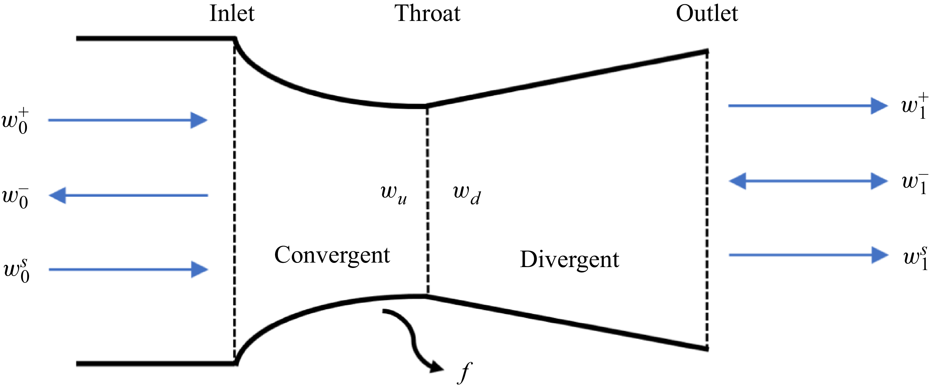
 f
f
 M
M T¯
T¯ f
f f
f

 w0−
w0− He
He f=0
f=0 f=0.015
 w1+
w1+ He
He f=0
f=0 f=0.015
 He
He f=0
f=0 f=0.015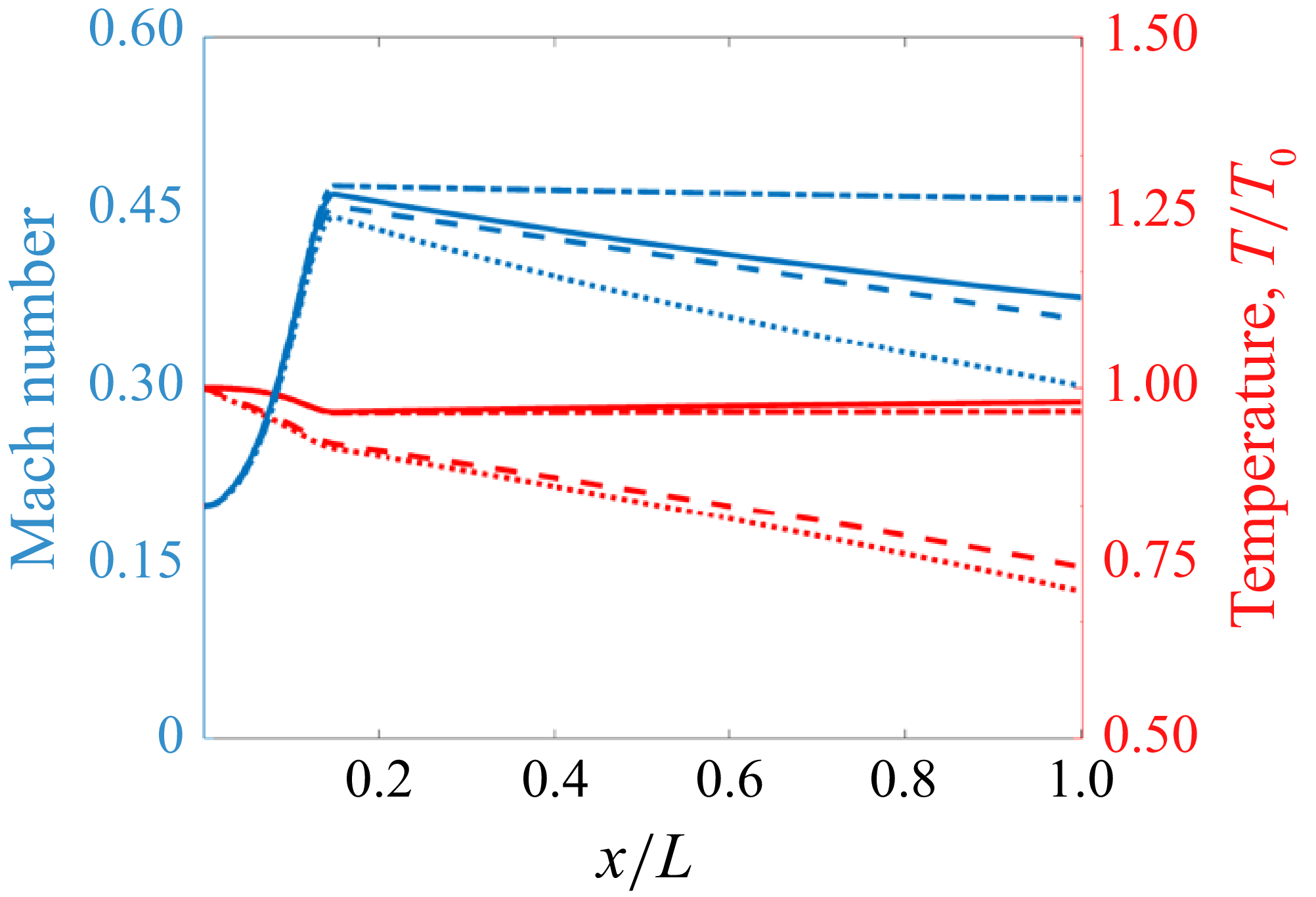
 M
M T¯
T¯ Q˙~=Q˙¯L/p¯0c¯0
 p¯0
p¯0 c¯0
c¯0 f=0
f=0 Q˙~=0
Q˙~=0 f=0.015
 Q˙~=0
Q˙~=0 f=0
f=0 Q˙~=
Q˙~= f=0.015
 Q˙~=
Q˙~=
 w0−
w0− He
He f=0.015
 Q˙~=0
Q˙~=0 f=0.015
 Q˙~=−0.35
 w1+
w1+ He
He f=0.015
 Q˙~=0
Q˙~=0 f=0.015
 Q˙~=−0.35
 Open access

