2.1. Basic notation

For two probability distributions $\mu, \nu$ on a common Polish probability space $(\Omega, \mathcal{F})$ , the total variation distance is defined by

\begin{align*} \| \mu - \nu \|_{\mathrm{TV}} = \sup_{A \in \mathcal{F}}|\mu(A) - \nu(A)|. \end{align*}

For $n \in \mathbb{N}$ , define $[n] = \{1,2,\ldots,n\}$ . By a small abuse of notation, we will sometimes treat a vector as a set (writing, for example, $x \in v$ rather than $x \in \{v_{1},\ldots,v_{n}\}$ ) when there is no possible ambiguity. We will frequently consider datasets $\{ X_{1},\ldots,X_{n} \}$ , and use $\mathcal{X}_{n} = \{ X_{1},\ldots,X_{n} \}$ to denote the full dataset.

2.2. Forward-mapping representation of subsampling MCMC

We consider the usual setup for Bayesian inference. We have a parameter space $(\Theta, \mathcal{F}_{\Theta})$ , a family of models $\{p(\cdot \mid\theta)\}_{\theta \in \Theta}$ , a prior p, and a dataset $\mathcal{X} = \{X_1,\ldots, X_n\}$ . For the entire paper, we assume that $(\Theta,d)$ is a Polish space and that $\mathcal{F}_{\Theta}$ is the usual Borel $\sigma$ -algebra.

We now define a family of ‘subsampling’ MCMC algorithms, which we will show contains many popular algorithms as special cases.

Fix a pair of probability spaces $(\mathbb{A},\mathcal{F}_{\mathbb{A}})$ and $(\Omega, \mathcal{F}_{\Omega})$ and a maximum ‘subsample size’ $m \in \mathbb{N}$ . Let $F \colon \Theta \times \mathbb{A} \times [n]^{m} \times \Omega \mapsto \Theta \times \mathbb{A} $ be a measurable function, let $\mu$ be a probability measure on $[n]^{m}$ , and let $\eta$ be a probability measure on $\Omega$ . The space $\Omega$ is used to capture all of the random variables sampled during a step of the underlying algorithm, except the choice of subsample. Typically, we can assume without loss of generality that this is of the form $[0,1]^{k}$ with the usual Borel $\sigma$ -algebra. 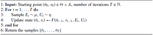These choices together define a forward-mapping representation for a Markov chain $\{\theta_{t}\}_{t \geq 0}$ via Algorithm 1.

Algorithm 1:

Sampling with explicit randomness.

One can check that this generic algorithm covers many popular subsampling algorithms, including stochastic gradient Langevin dynamics (see [Reference Welling and Teh21]) and subsampling pseudo-marginal Metropolis–Hastings (see [Reference Quiroz, Villani and Kohn16]). The auxiliary variable $r_{t}$ allows us to include popular algorithms such as stochastic gradient Hamiltonian Monte Carlo [Reference Chen, Fox and Guestrin6] or the pseudo-marginal algorithm [Reference Andrieu and Roberts1] in the form of Algorithm 1.

As a concrete example, the following gives a representation of the usual SGLD algorithm on $\mathbb{R}^{d}$ .

Example 1. Fix dimension $d \in \mathbb{N}$ , step size $\epsilon \gt 0$ , and subsample size $m = m(\theta) \leq M$ . Then SGLD (with the usual Euler–Maruyama discretization) can be written in the form of Algorithm 1 with the choices

(1) \begin{equation} \mathbb{A} = \emptyset, \quad \Omega = \mathbb{R}^{d}, \quad \eta = N(0,\mathbf{1}_{d}), \quad \mu = \mathrm{Unif}([n]^{M}),\end{equation}

and

(2) \begin{equation} F(\theta,r,E,U) = \theta + \dfrac{\epsilon}{2}\Biggl(\nabla \log p(\theta) + \dfrac{n}{m(\theta)}\sum_{j = 1}^{m(\theta)} \nabla\log p(X_{E[j]} \mid \theta)\Biggr) + \sqrt{\epsilon} \, U.\end{equation}

The main constraint comes from the restriction to independent and identically distributed (i.i.d.) selection of subsamples, which excludes some algorithms with complex subsample selection mechanisms (see e.g. [Reference Quiroz, Villani, Kohn, Tran and Dang17] for a survey of approaches). We will show in later sections how some algorithms that do this can still be placed in the framework of this paper (see Remark 1).

2.3. Perturbations of posterior distributions of exponential families

We focus on exponential families with likelihoods of the form

(3) \begin{equation} p(x \mid \theta) = h(x)\exp(\theta R(x) - A(\theta)),\end{equation}

where $x \in \mathbb{R}$ , h and R are real-valued functions, and A is the associated log-normalizing constant. Fixing a prior p on $\Theta$ , the associated posterior density is given by

\begin{align*} p(\theta \mid \mathcal{X}_{n}) = \dfrac{\exp(\theta S - nA(\theta))p(\theta)}{\int \exp(\theta' S - nA(\theta')) p(\theta')\,{\mathrm{d}} \theta'},\end{align*}

where $S = \sum_{i=1}^n R(X_i)$ is the sufficient statistic.

We then consider the ‘perturbed’ posterior associated with a ‘perturbed’ sufficient statistic $S + n\delta$ :

\begin{align*} p_\delta(\theta \mid \mathcal{X}_{n}) = \dfrac{\exp(\theta (S + n\delta) - nA(\theta))p(\theta)} {\int \exp(\theta' (S + n\delta) - nA(\theta')) p(\theta')\,{\mathrm{d}} \theta'}.\end{align*}

We will use the following perturbation assumption on the likelihood when analyzing MCMC on ‘small’ time intervals.

Assumption 1. There exists $\gamma \gt 0$ so that for all sequences $c_{n} \rightarrow \infty$ , all datasets $X_{1},X_{2},\ldots,$ and all sequences $|\delta_{n}| \gt {{c_{n}}/{\sqrt{n}}}$ ,

\begin{align*}\liminf_{n \rightarrow \infty} \| p(\theta \mid \mathcal{X}_{n}) - p_{\delta_{n}}(\theta \mid \mathcal{X}_{n}) \|_{\mathrm{TV}} \geq \gamma.\end{align*}

This condition says that the posterior distribution is somewhat sensitive to large changes in the data. This assumption holds with $\gamma = 1$ when the posterior distribution is close to Gaussian, as well as in many other situations. See Appendix A.1 for a simple condition under which Assumption 1 holds with high probability, and which is based only on the first two moments of the posterior. Appendix A.1 also contains an application of this sufficient condition to show that the Gaussian model satisfies this condition with $\gamma = 1$ .

Assumption 1 is relevant to small time scales. On large time scales, we consider smaller perturbations, leading to the following assumption.

Assumption 2. There exists $\gamma \gt 0$ so that for all sequences $c_{n} \rightarrow 0$ , all datasets $X_{1},X_{2},\ldots,$ and all sequences $\delta_{n} \lt {{c_{n}}/{\sqrt{n}}}$ ,

\begin{align*}\liminf_{n \rightarrow \infty} \dfrac{\| p(\theta \mid \mathcal{X}_{n}) - p_{\delta_{n}}(\theta \mid \mathcal{X}_{n}) \|_{\mathrm{TV}}}{\delta_{n}} \geq \gamma.\end{align*}

Again, this assumption is easy to verify for posterior distributions that are near-Gaussian, and it holds in substantial generality. See Appendix A.2 for a quick proof and related calculations.

3.1. Coupling construction for SGLD

We consider the representation of SGLD given in Example 1. In this section, we construct a coupling of two Markov chains to ensure that they remain far apart with high probability. This construction represents the main observation behind our main result: it is possible to couple the choice of subsamples across two chains so that the two chains are quite close in total variation, but certain functionals are somewhat far in expectation.

We begin by constructing a distribution $\nu$ that is close (in total variation distance) to the distribution $\mu$ used in Example 1. Fix a parameter $\delta \gt 0$ and $M,n \in \mathbb{N}$ with $M \leq n$ ; n remains the size of the dataset, and we think of M as the subsample size for SGLD. Sample $E[1],\ldots,E[M] \stackrel{\mathrm{i.i.d.}}{\sim} \mathrm{Unif}(\{1,2,\ldots,n\})$ , then independently sample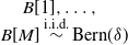 $B[1],\ldots, B[M] \stackrel{\mathrm{i.i.d.}}{\sim} \mathrm{Bern}(\delta)$ and $E^{+}[1],\ldots,E^{+}[M] \stackrel{\mathrm{i.i.d.}}{\sim} \mathrm{Unif}(\{\lceil {{n}/{2}} \rceil,\ldots,n\}) $ . Finally, for $i \in \{1,2,\ldots,M\}$ , set

\begin{align*}D[i] = \begin{cases} E[i], & B[i] = 0, \\[3pt] E^{+}[i], & B[i] = 1. \end{cases} \end{align*}

Let $\nu = \nu_{M,\delta}$ denote the distribution of the vector D and let $\mu = \mu_{M}$ be the distribution of the vector E.

Recall that sampling $E_{t} \sim \mu_{M} \equiv \mathrm{Unif}([n]^{M})$ gives the SGLD algorithm in equations (1) to (2), targeting the posterior $p(\theta \mid x)$ . If we were to replace $\mu_{M}$ with $\nu_{M,\delta}$ in the algorithm, this construction turns out to give another valid SGLD algorithm; but targeting a certain ‘weighted’ posterior distribution. More precisely, we have the following result.

Lemma 1. (Weighted gradient estimation.) Fix $0 \lt \delta <1$ , sample the set $D \sim \nu_{M,\delta}$ , and define $w_i = \mathbb{P}(D[1] = i)$ for $i \in \{1,\ldots, n\}$ . Then

\begin{align*} \mathbb{E}\Biggl[ \dfrac{n}{M}\sum_{j \in D} \nabla \log p(X_{j} \mid \theta) \Biggr] = \sum_{i=1}^{n} n \, w_i\nabla \log p(X_i \mid \theta).\end{align*}

Proof. For all j, we have by the definition of $w_i$ that

\begin{align*} \mathbb{E}[n \nabla \log p(X_{D[1]} \mid \theta)] = \sum_{i=1}^n n \,w_i\nabla \log p(X_i \mid \theta).\end{align*}

The result follows from linearity of expectation.

We interpret this as saying that

\begin{align*}\frac{n}{M}\sum_{j \in D} \nabla \log p(X_{j} \mid \theta) \end{align*}

is an unbiased estimator for the gradient of the log-likelihood for the weighted model

\begin{align*}\prod_{i=1}^n p(X_i \mid \theta)^{nw_i}. \end{align*}

For later reference, if $D\sim\nu_{M,\omega}$ , $0<\omega<1$ , and $s=\lceil n/2\rceil$ , then the weights are

\begin{equation*} w_i^{(n,\omega)}=\dfrac{1-\omega}{n}+\dfrac{\omega}{n-s+1}{\mathbf{1}}_{\{i\geq s\}}.\end{equation*}

Define

(4) \begin{equation}\Pi_{n,\omega}^{\mathrm{wt}}(\theta\mid \mathcal{X}_{n})\propto p(\theta)\prod_{i=1}^n p(X_i\mid\theta)^{n w_i^{(n,\omega)}}.\end{equation}

For the exponential family (3), this is the same as

(5) \begin{equation}\Pi_{n,\omega}^{\mathrm{wt}}(\cdot\mid \mathcal{X}_{n})=p_{\delta_n^{\mathrm{wt}}(\omega)}(\cdot\mid \mathcal{X}_{n}),\quad\delta_n^{\mathrm{wt}}(\omega)=\omega\Biggl(\dfrac{1}{n-s+1}\sum_{i=s}^{n}R(X_i)-\dfrac{1}{n}\sum_{i=1}^{n}R(X_i)\Biggr).\end{equation}

We can now couple samples from the original and ‘perturbed’ SGLD algorithm.

Lemma 2. There exists a universal constant C with the following property. Fix

\begin{align*}M \in \mathbb{N},\quad 0 \lt \alpha \lt \frac{1}{2},\quad 0 \lt \delta \lt \frac{1}{2}\min \biggl(1,\frac{C \alpha^{2}}{ \sqrt{M}}\biggr). \end{align*}

Then

\begin{align*}\| \mu_{M} - \nu_{M,\delta} \|_{TV} \leq \alpha.\end{align*}

Proof. We use a calculation that is very similar to the proof in Section 1.3 of [Reference Chatterjee5]. Let $D \sim \mu_{M}$ and $E \sim \nu_{M,\delta}$ . Let $s =\lceil {{n}/{2}} \rceil$ , let $p = P[E[1] \geq s] - \frac{1}{2}$ and $q = \frac{1}{2} - P[E[1] \lt s]$ be the ‘bias’ induced by $\nu_{M,\delta}$ . Let $D^{+} = \{i \in [M] \colon D[i] \geq s\}$ and $E^{+} = \{i \in [M] \colon E[i] \geq s\}$ .

We are interested in counting the number of times that points with large index are chosen. Let f be the density of the distribution $\mathcal{L}(|D^{+}|)$ with respect to $\mathcal{L}(|E^{+}|)$ . We then have

\begin{align*}f(D) = \biggl(\dfrac{1}{2} + p\biggr)^{|D^{+}|} \biggl(\dfrac{1}{2}-q\biggr)^{M-|D^{+}|} = \biggl[\biggl(\dfrac{1}{2}+p\biggr)\biggl(\dfrac{1}{2}-q\biggr)\biggr]^{{{M}/{2}}} \biggl(\dfrac{1+2p}{1-2q}\biggr)^{|D^{+}|-{{M}/{2}}}.\end{align*}

Thus

\begin{align*}\| \mu_{M} - \nu_{M,\delta} \|_{TV} \leq \mathbb{E}\biggl[\biggl(1 - \biggl[\biggl(\dfrac{1}{2}+p\biggr)\biggl(\dfrac{1}{2}-q\biggr)\biggr]^{{{M}/{2}}} \biggl(\dfrac{1+2p}{1-2q}\biggr)^{D^{+}-{{M}/{2}}} \biggr)_{+} \biggr].\end{align*}

Note that $D^{+}$ is a binomial random variable. Applying Chebyshev’s inequality to $D^{+}$ , the same calculation as in Section 1.3 of [Reference Chatterjee5] says that there exists a universal constant $C \gt 0$ so that

\begin{align*}\| \mu_{M} - \nu_{M,\delta} \|_{TV} \leq C \sqrt{\alpha}.\end{align*}

This completes the proof.

We now wish to establish that this small perturbation of the driving randomness corresponds to a similarly sized perturbation of the sufficient statistics in the effective model. We have the following result.

Lemma 3. Fix $\delta \gt 0$ , $M \in \mathbb{N}$ and a non-decreasing sequence $X_{1} \leq X_{2} \leq \cdots \leq X_{n}$ . Let $s = \lceil {{n}/{2}}\rceil$ . Let $E \sim \mu_{M}$ and $D \sim \nu_{M, \delta}$ . Then

\begin{align*}\mathbb{E}\Biggl[\dfrac{1}{M}\sum_{j=1}^{M} R(X_{D[j]}) - \dfrac{1}{M}\sum_{j=1}^{M} R(X_{E[j]}) \Biggr]= \delta \Biggl(\dfrac{1}{n-s+1} \sum_{i = s}^{n} R(X_{i}) - \dfrac{1}{n} \sum_{i =1}^{n} R(X_{i}) \Biggr).\end{align*}

We add the (very weak) assumption that this is large with high probability.

Assumption 3. A likelihood of the form (3) and parameter $\theta_{0}$ have the following property.

Fix $n \in \mathbb{N}$ , let $s = \lceil {{n}/{2}} \rceil$ , let $Y_{1},Y_{2},\ldots, Y_{n} \stackrel{\mathrm{i.i.d.}}{\sim} p(\cdot \mid \theta_{0})$ , and let $X_{1} \leq X_{2} \leq \cdots \leq X_{n}$ be the same points put in ascending order. Then

\begin{equation*}\lim_{n \rightarrow \infty} \mathbb{P}\Biggl[\Biggl| \dfrac{1}{n-s+1} \sum_{i = s}^{n} R(X_{i}) - \dfrac{1}{n} \sum_{i =1}^{n} R(X_{i}) \Biggr| \lt \eta \Biggr] = 0.\end{equation*}

This assumption is quite weak, and is straightforward to check for popular functions R. To give a concrete example, when $R(x) = x$ , this follows immediately from Chebyshev’s inequality.

3.2. Lower bounds for short runs

We set notation for the main result. Fix a prior p and model $p(\cdot \mid x)$ . For fixed dataset X and sample size M, let $K_{X,M}$ denote the transition kernel associated with the SGLD algorithm in Example 1. Similarly, for fixed $\delta \gt 0$ , let $K_{X,\delta,M}$ denote the transition kernel associated with the SGLD algorithm in Example 1, with $\mu_{M}$ replaced by $\nu_{M,\delta}$ .

Finally, we set sequences of integers $T_{n}$ and (possibly time-inhomogeneous) batch sizes $m_{n,1},\ldots,m_{n,T_{n}}$ and perturbation sizes $\omega_{n}$ , and define the total number of sampled datapoints

(6) \begin{equation} G_{n} = \sum_{t=1}^{T_{n}} m_{n,t}.\end{equation}

In the following theorem, we will assume that

(7) \begin{equation} \lim_{n \rightarrow \infty} \dfrac{G_{n}}{n} = 0\end{equation}

and

(8) \begin{equation} \lim_{n\rightarrow \infty} \omega_{n} \sqrt{G_{n}} = 0, \quad \lim_{n\rightarrow \infty} \omega_{n} \sqrt{n} = \infty.\end{equation}

Our main result is as follows.

Theorem 1. Fix a prior p, likelihood $p(\cdot \mid \theta)$ and parameter value $\theta_{0}$ satisfying Assumptions 1 and 3. Let $Y_{1},Y_{2},\ldots \stackrel{\mathrm{i.i.d.}}{\sim} p(\cdot \mid \theta_{0})$ be data sampled from this. For each n, let $X_{1}\leq \cdots \leq X_{n}$ be $Y_1,\ldots,Y_n$ put in ascending order. Let $T_{n}\in\mathbb{N}$ , step sizes $\epsilon_{n,1},\ldots,\epsilon_{n,T_{n}}>0$ , perturbation sizes $\omega_{n}$ and batch sizes $m_{n,1},\ldots,m_{n,T_{n}}\in\{1,\ldots,n\}$ be deterministic (depending only on n), and let $G_{n}$ be as in (6). Assume equations (7) and (8) hold.

Let $Z_{1}^{(n)},Z_{2}^{(n)},\ldots,Z_{T_{n}}^{(n)}$ be generated by Algorithm 1 with the SGLD update maps of Example 1, using $\epsilon_{t}=\epsilon_{n,t}$ and using only the first $m_{n,t}$ entries of the selection variable $E_{t}$ at time t. Similarly, let $\tilde{Z}_{1}^{(n)},\ldots,\tilde{Z}_{T_{n}}^{(n)}$ be generated in the same way, but with the selection variable $E_{t}$ sampled from the perturbed law corresponding to $\omega_{n}$ (i.e. with $\mu_{M}$ replaced by $\nu_{M,\omega_{n}}$ in the construction of $E_{t}$ ) for every datapoint query. Then, for all $a \gt 0$ ,

\begin{equation*}\lim_{n \rightarrow \infty} \mathbb{P}\bigl[\bigl\|\mathcal{L}\bigl(Z_{T_{n}}^{(n)}\bigr) - p(\cdot \mid \mathcal{X}_{n})\bigr\|_{\mathrm{TV}} + \bigl\|\mathcal{L}\bigl(\tilde{Z}_{T_{n}}^{(n)}\bigr) - \Pi_{n,\omega_{n}}^{\mathrm{wt}}(\cdot \mid \mathcal{X}_{n})\bigr\|_{\mathrm{TV}} \geq (1-a)\gamma\bigr] = 1.\end{equation*}

Proof. For fixed n, let $\mathcal{E}_{n}$ denote the event that

\begin{equation*}\Biggl| \dfrac{1}{n-s+1} \sum_{i = s}^{n} R(X_{i}) - \dfrac{1}{n} \sum_{i =1}^{n} R(X_{i}) \Biggr| \geq \eta,\end{equation*}

where $s = \lceil {{n}/{2}} \rceil$ .

We first check that the target distributions of our algorithms are far. Combining Lemma 1, Lemma 3, and (5), on the event $\mathcal{E}_{n}$ we have

(9) \begin{equation} \liminf_{n \rightarrow \infty} \| p(\cdot \mid \mathcal{X}_{n}) - \Pi_{n,\omega_{n}}^{\mathrm{wt}}(\cdot \mid \mathcal{X}_{n}) \|_{\mathrm{TV}} \geq \gamma.\end{equation}

We next check that the samples of our algorithms are close. Let $\mathbf{E}^{(n)}$ denote the concatenation of all indices actually queried by the first run, i.e. the vector in $[n]^{G_{n}}$ obtained by concatenating $E_{t}[1],\ldots,E_{t}[m_{n,t}]$ over $t=1,\ldots,T_{n}$ , and define $\tilde{\mathbf{E}}^{(n)}$ analogously for the perturbed run. Then $\mathbf{E}^{(n)} \sim \mu_{G_{n}}$ and $\tilde{\mathbf{E}}^{(n)} \sim \nu_{G_{n},\omega_{n}}$ . By Lemma 2 and (8), we may couple $\mathbf{E}^{(n)}$ and $\tilde{\mathbf{E}}^{(n)}$ so that $\mathbb{P}[\mathbf{E}^{(n)} \neq \tilde{\mathbf{E}}^{(n)}]\to 0$ . Coupling also the Gaussian noises $\{U_t\}$ identically across the two runs, the forward-mapping representation implies that the full trajectories coincide with probability tending to 1:

(10) \begin{equation} \lim_{n \rightarrow \infty} \mathbb{P}\bigl[\bigl(Z_{1}^{(n)},\ldots,Z_{T_{n}}^{(n)}\bigr) = \bigl(\tilde{Z}_{1}^{(n)},\ldots,\tilde{Z}_{T_{n}}^{(n)}\bigr)\bigr] = 1.\end{equation}

Next, by the triangle inequality,

\begin{align*}\Delta_{n} &\equiv \bigl\|\mathcal{L}\bigl(Z_{T_{n}}^{(n)}\bigr) - p(\cdot \mid \mathcal{X}_{n})\bigr\|_{\mathrm{TV}} + \bigl\|\mathcal{L}\bigl(\tilde{Z}_{T_{n}}^{(n)}\bigr) - \Pi_{n,\omega_{n}}^{\mathrm{wt}}(\cdot \mid \mathcal{X}_{n})\bigr\|_{\mathrm{TV}} \\[3pt]& \geq \| p(\cdot \mid \mathcal{X}_{n}) - \Pi_{n,\omega_{n}}^{\mathrm{wt}}(\cdot \mid \mathcal{X}_{n})\|_{\mathrm{TV}} - \bigl\| \mathcal{L}\bigl(Z_{T_{n}}^{(n)}\bigr) - \mathcal{L}\bigl(\tilde{Z}_{T_{n}}^{(n)}\bigr) \bigr\|_{\mathrm{TV}}.\end{align*}

Applying (10) and (9) to the terms on the right-hand side of this inequality, we have for all $a \gt 0$

\begin{align*}\lim_{n \rightarrow \infty} \mathbb{P}[\Delta_{n} \lt (1-a)\gamma] \leq \lim_{n \rightarrow \infty} \mathbb{P}[\mathcal{E}_{n}^{c}].\end{align*}

By Assumption 3, this last limit is 0, completing the proof.

3.3. Lower bounds with strong control variates

Theorem 1 gave a lower bound on the error of a naive SGLD algorithm. It is known that naive SGLD can fail catastrophically (see [Reference Brosse, Durmus and Moulines4] for a typical example in which the stationary distribution is very far from the ostensible target), and so in practice it is common to use control variates that are highly informative but not quite sufficient statistics. In this section, we give lower bounds on the error rate of SGLD for a toy model of this situation: a log-likelihood that is the sum of one dominant term that is used as a control variate, and a second lower-order term that is estimated from the data. In this regime, the stationary measure of SGLD will converge to the ‘right’ answer as n goes to infinity, and we obtain lower bounds that depend on the error in the second-order term. Informally, we view these as being similar to Theorem 1: the accuracy of SGLD cannot improve upon some natural baseline until a large fraction of the data has been used.

Let $\theta=(\theta^{(1)},\theta^{(2)})\in\Theta\subseteq\mathbb{R}^{2}$ and consider the two-parameter exponential family

\begin{equation*} p(x\mid \theta)=\exp\bigl(\theta^{(1)}R_{1}(x)+\theta^{(2)}R_{2}(x)-A(\theta)\bigr)p_{0}(x).\end{equation*}

For data $\mathcal{X}_{n}=\{X_{1},\ldots,X_{n}\}$ , define sufficient statistics

\begin{align*}S_{1}=\sum_{i=1}^{n}R_{1}(X_{i}),\quad S_{2}=\sum_{i=1}^{n}R_{2}(X_{i}), \end{align*}

scaling parameter $\alpha_{n}$ , and pseudo-posterior

\begin{equation*} p(\theta\mid \mathcal{X}_{n}) \propto \exp\bigl(\theta^{(1)}S_{1}+\alpha_{n}\,\theta^{(2)}S_{2}-nA(\theta)\bigr)p(\theta).\end{equation*}

We consider an SGLD-like algorithm in which $S_{1}$ is available exactly for use as a control variate, while $S_{2}$ is estimated by subsampling.

Example 2. (Simple SGLD with control variates.) Fix step sizes $\epsilon_{t}>0$ and batch sizes $m_{t}\in\{1,\ldots,n\}$ . At time t, sample indices $E_{t}[1],\ldots,E_{t}[m_{t}]$ i.i.d. from $\mathrm{Unif}(\{1,\ldots,n\})$ and define

\begin{align*}\widehat{S}_{2,t}\, :\!= \, \dfrac{n}{m_{t}}\sum_{j=1}^{m_{t}}R_{2}(X_{E_{t}[j]}). \end{align*}

With i.i.d. $U_{t}\sim N(0,\mathbf{1}_{d})$ , update

\begin{equation*} \theta_{t}=\theta_{t-1}+\dfrac{\epsilon_{t}}{2}(\nabla\log p(\theta_{t-1})+(S_{1} ,\alpha_{n}\,\widehat{S}_{2,t})-n\nabla A(\theta_{t-1}))+\sqrt{\epsilon_{t}}\,U_{t}.\end{equation*}

3.3.1. Short-run lower bound.

For $\delta\in\mathbb{R}$ , define the ‘second-statistic perturbed posterior’

\begin{equation*} p^{(2)}_{\delta}(\theta\mid \mathcal{X}_{n}) \propto \exp\bigl(\theta^{(1)}S_{1}+\alpha_{n}\,\theta^{(2)}(S_{2}+n\delta)-nA(\theta)\bigr)p(\theta).\end{equation*}

We use the following analog of Assumption 1 for perturbations in the $R_{2}$ -statistic.

Assumption 4. There exist constants $c, \gamma_{2} \gt 0$ , and a deterministic sequence $\beta_{n}\downarrow 0$ so that for all datasets $\mathcal{X}_{n}$ and all sequences $\delta_{n} \gt {{c}/{\sqrt{n}}}$ ,

\begin{align*}\liminf_{n \rightarrow \infty} \dfrac{\big\| p(\cdot \mid \mathcal{X}_{n}) - p^{(2)}_{\delta_{n}}(\cdot \mid \mathcal{X}_{n}) \big\|_{\mathrm{TV}}}{\beta_{n}} \geq \gamma_{2}. \end{align*}

We also use the obvious analog of Assumption 3, again applied to $R_{2}$ .

Assumption 5. There exists $\eta>0$ such that, letting $s=\lceil n/2\rceil$ and letting $X_{1}\le \cdots \le X_{n}$ denote the ordered sample from $p(\cdot\mid \theta_{0})$ , we have

\begin{align*}\lim_{n \rightarrow \infty} \mathbb{P}\Biggl[\Biggl| \dfrac{1}{n-s+1} \sum_{i = s}^{n} R_{2}(X_{i}) - \dfrac{1}{n} \sum_{i =1}^{n} R_{2}(X_{i}) \Biggr| \lt \eta \Biggr] = 0. \end{align*}

Fix sequences $T_{n}$ and batch sizes $m_{n,1},\ldots,m_{n,T_{n}}$ and define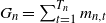 $G_{n}=\sum_{t=1}^{T_{n}}m_{n,t}$ . Consider two runs of Example 2 with identical step sizes and Gaussian noises, but with different index laws:

1. (i) the uniform run draws all queried indices i.i.d. from $\mathrm{Unif}(\{1,\ldots,n\})$ ;

2. (ii) the perturbed run draws all queried indices i.i.d. from the one-sample mixture corresponding to parameter $\omega_{n}$ .

Define the (data-dependent) perturbation size, where $s=\lceil n/2\rceil$ ,

\begin{align*}\delta^{(2)}_{n}\, :\!= \, \omega_{n}\Biggl(\dfrac{1}{n-s+1}\sum_{i=s}^{n}R_{2}(X_{i})-\dfrac{1}{n}\sum_{i=1}^{n}R_{2}(X_{i})\Biggr). \end{align*}

We are ready to state our analog of Theorem 1. We emphasize that there is one substantial difference: the lower bound scales like $\beta_{n}$ rather than as a constant. This should be unsurprising. Since $S_{2}$ contains less information than $S_{1}$ , even MCMC based only on the known value of $S_{1}$ would result in an error that goes to 0 with n, at a rate that depends on $\beta_{n}$ . Our result shows that one needs to see a substantial fraction of the data to improve on this control-variate-only estimate.

Theorem 2. Fix notation as in the statement of Theorem 1, except for the following changes. Replace Assumptions 1 and 3 with Assumptions 4 and 5. Replace the conditions on $G_{n}, \omega_{n}$ with the assumption that $G_{n}/n\to 0$ , $\omega_{n}\sqrt{G_{n}}\to 0$ , $\liminf_{n\to\infty} \omega_{n}\sqrt{n} \gt 0$ and $\omega_{n}^{{{1}/{2}}} (G_{n})^{{{1}/{4}}} = {\mathrm{o}}(\beta_{n})$ . Let $Z_{T_{n}}^{(n)}$ be the output of the uniform run and $\tilde Z_{T_{n}}^{(n)}$ the output of the perturbed run.

Then, for all $a>0$ ,

\begin{align*}\lim_{n \rightarrow \infty} \mathbb{P}\bigl[\bigl\|\mathcal{L}\bigl(Z_{T_{n}}^{(n)}\bigr) - p(\cdot \mid \mathcal{X}_{n})\bigr\|_{\mathrm{TV}} + \bigl\|\mathcal{L}\bigl(\tilde{Z}_{T_{n}}^{(n)}\bigr) - p^{(2)}_{\delta^{(2)}_{n}}(\cdot \mid \mathcal{X}_{n})\bigr\|_{\mathrm{TV}} \geq (1-a)\gamma_{2} \beta_{n} \bigr] = 1. \end{align*}

Proof. The proof is the same as the proof of Theorem 1, with R replaced by $R_{2}$ and with $p_{\delta}$ replaced by $p^{(2)}_{\delta}$ . We sketch the two main changes.

1. (i) Targets are far. By Lemma 3 applied to $R_{2}$ and the definition of $\delta^{(2)}_{n}$ , on the event in Assumption 5 we have $|\delta^{(2)}_{n}|\ge \omega_{n}\eta$ . Since $\liminf_{n\to\infty}\omega_{n}\sqrt{n}>0$ , this implies $|\delta^{(2)}_{n}|>{{c}/{\sqrt{n}}}$ , and hence Assumption 4 yields a total-variation separation of at least $\gamma_{2}\beta_{n}$ between $p(\cdot\mid \mathcal{X}_{n})$ and $p^{(2)}_{\delta^{(2)}_{n}}(\cdot\mid \mathcal{X}_{n})$ with probability tending to 1.

2. (ii) Samples are close. By Lemma 2, together with the assumption $\omega_{n}^{{{1}/{2}}} (G_{n})^{{{1}/{4}}}={\mathrm{o}}(\beta_{n})$ , we may couple the concatenated index vectors so that they agree with probability $1-{\mathrm{o}}(\beta_{n})$ . Coupling the Gaussian noises identically and using the forward-mapping representation then implies that the two trajectories agree with probability $1-{\mathrm{o}}(\beta_{n})$ . The triangle inequality completes the argument exactly as in the proof of Theorem 1.

Remark 5. In typical near-Gaussian settings, we expect the best choice of $\beta_{n}$ in Assumption 4 to scale proportionally to $\alpha_{n}$ for perturbations of size $\delta_{n}\asymp 1/\sqrt{n}$ . In that case, the additional condition $\omega_{n}^{{{1}/{2}}} (G_{n})^{{{1}/{4}}}={\mathrm{o}}(\beta_{n})$ simply requires that the coupling error in the subsample indices is negligible at the scale of the $S_{2}$ -induced posterior shift.

3.4. Lower bounds for long runs

We give results that are very similar to those of Theorem 1, but for longer time scales. We use the same notation as that immediately preceding the statement of Theorem 1, but replace conditions (7) and (8) with

(11) \begin{equation} \lim_{n \rightarrow \infty} \dfrac{G_{n}}{n} = \infty\end{equation}

and

(12) \begin{equation} \lim_{n\rightarrow \infty} \omega_{n} \sqrt{G_{n}} = 0.\end{equation}

Lemma 4. There exists a universal constant $C_{\mathrm{coup}}>0$ such that the following holds. Fix $G\in\mathbb{N}$ and $0<\delta<\tfrac12$ . Let $\mathbf{E}\sim \mu_{G}$ and $\mathbf{D}\sim \nu_{G,\delta}$ . Then

\begin{align*}\|\mu_{G}-\nu_{G,\delta}\|_{\mathrm{TV}}\le C_{\mathrm{coup}}\,\delta^{{{1}/{2}}}\,G^{{{1}/{4}}}. \end{align*}

In particular, there exists a coupling of $\mathbf{E}$ and $\mathbf{D}$ such that $\mathbb{P}[\mathbf{E}\neq \mathbf{D}]\le C_{\mathrm{coup}}\,\delta^{{{1}/{2}}}\,G^{{{1}/{4}}}$ .

The proof is quite similar to the proof of Theorem 1.

Theorem 3. Fix notation as in the statement of Theorem 1, with the following changes. Replace Assumption 1 with Assumption 2. Replace the conditions on $\omega_{n}, G_{n}$ with equations (11) and (12).

Then, for all $a \gt 0$ ,

\begin{equation*}\lim_{n \rightarrow \infty} \mathbb{P}\bigl[\bigl\|\mathcal{L}\bigl(Z_{T_{n}}^{(n)}\bigr) - p(\cdot \mid \mathcal{X}_{n})\bigr\|_{\mathrm{TV}} + \bigl\|\mathcal{L}\bigl(\tilde{Z}_{T_{n}}^{(n)}\bigr) - \Pi_{n,\omega_{n}}^{\mathrm{wt}}(\cdot \mid \mathcal{X}_{n})\bigr\|_{\mathrm{TV}} \geq (1-a)\gamma\bigr] = 1.\end{equation*}

Proof. For fixed n, let $\mathcal{E}_{n}$ denote the event that

\begin{equation*}\Biggl| \dfrac{1}{n-s+1} \sum_{i = s}^{n} R(X_{i}) - \dfrac{1}{n} \sum_{i =1}^{n} R(X_{i}) \Biggr| \geq \eta,\end{equation*}

where $s = \lceil {{n}/{2}} \rceil$ .

We first check that the target distributions of our algorithms are far. Combining Lemma 1, Lemma 3, and (5), on the event $\mathcal{E}_{n}$ we have

(13) \begin{equation} \liminf_{n \rightarrow \infty} \, \omega_{n}^{-1} \| p(\cdot \mid \mathcal{X}_{n}) - \Pi_{n,\omega_{n}}^{\mathrm{wt}}(\cdot \mid \mathcal{X}_{n}) \|_{\mathrm{TV}} \geq \eta \, \gamma.\end{equation}

We next check that the samples of our algorithms are close.

Let $\mathbf{E}^{(n)}\in [n]^{G_{n}}$ denote the concatenation of all indices queried by the original run (i.e. the concatenation of the first $m_{n,t}$ entries of $E_{t}$ over $t=1,\ldots,T_{n}$ ), and let $\mathbf{D}^{(n)}\in [n]^{G_{n}}$ denote the analogous concatenation for the perturbed run. By Lemma 4, we may couple $\mathbf{E}^{(n)}$ and $\mathbf{D}^{(n)}$ so that

\begin{align*}\mathbb{P}[\mathbf{E}^{(n)}\neq \mathbf{D}^{(n)}]\le C_{\mathrm{coup}}\,\omega_{n}^{{{1}/{2}}}\,G_{n}^{{{1}/{4}}}. \end{align*}

Coupling also the Gaussian noises identically across the two runs and using the forward-mapping representation, it follows that under this coupling

(14) \begin{equation} \mathbb{P}\bigl[\bigl(Z_{1}^{(n)},\ldots,Z_{T_{n}}^{(n)}\bigr) \neq \bigl(\tilde{Z}_{1}^{(n)},\ldots,\tilde{Z}_{T_{n}}^{(n)}\bigr)\bigr]\le C_{\mathrm{coup}}\,\omega_{n}^{{{1}/{2}}}\,G_{n}^{{{1}/{4}}},\end{equation}

where $C_{\mathrm{coup}}$ is the constant from Lemma 4. Next, by the triangle inequality,

\begin{align*}\Delta_{n} &\equiv \bigl\|\mathcal{L}\bigl(Z_{T_{n}}^{(n)}\bigr) - p(\cdot \mid \mathcal{X}_{n})\bigr\|_{\mathrm{TV}} + \bigl\|\mathcal{L}\bigl(\tilde{Z}_{T_{n}}^{(n)}\bigr) - \Pi_{n,\omega_{n}}^{\mathrm{wt}}(\cdot \mid \mathcal{X}_{n})\bigr\|_{\mathrm{TV}} \\[3pt]& \geq \| p(\cdot \mid \mathcal{X}_{n}) - \Pi_{n,\omega_{n}}^{\mathrm{wt}}(\cdot \mid \mathcal{X}_{n})\|_{\mathrm{TV}} - \bigl\| \mathcal{L}\bigl(Z_{T_{n}}^{(n)}\bigr) - \mathcal{L}\bigl(\tilde{Z}_{T_{n}}^{(n)}\bigr) \bigr\|_{\mathrm{TV}}.\end{align*}

Applying inequalities (14) and (13) to the terms on the right-hand side of this inequality, we have for all $a \gt 0$

\begin{align*}\lim_{n \rightarrow \infty} \mathbb{P}\bigl[\Delta_{n} \lt \eta\gamma\,\omega_{n} - C_{\mathrm{coup}} \,\omega_{n}^{{{1}/{2}}}(G_{n})^{{{1}/{4}}}\bigr] \leq \lim_{n \rightarrow \infty} \mathbb{P}[\mathcal{E}_{n}^{c}].\end{align*}

By Assumption 3, this last limit is 0, so for all $ a \gt 0$

\begin{align*}\lim_{n \rightarrow \infty} \mathbb{P}\bigl[\Delta_{n} \lt (1-a)\eta\gamma \omega_{n} + \bigl(a \eta\gamma \omega_{n} - C_{\mathrm{coup}} \omega_{n}^{{{1}/{2}}} (G_{n})^{{{1}/{4}}}\bigr) \bigr] = 0.\end{align*}

By assumption (12),

\begin{equation*}\liminf_{ n \rightarrow \infty} \bigl(a \eta\gamma \omega_{n} - C_{\mathrm{coup}} \omega_{n}^{{{1}/{2}}} (G_{n})^{{{1}/{4}}}\bigr) \geq 0,\end{equation*}

so this completes the proof.