


1. Introduction
Fully developed turbulence exhibits strong spatio-temporal fluctuations over a wide range of scales. As a consequence, if physical quantities of turbulence, such as the velocity and transported scalars, are measured at a fixed point in space, a time series with occasional and transient intense localized peaks could be obtained (Batchelor & Townsend Reference Batchelor and Townsend1949). This phenomenon is known as turbulent intermittency and has been demonstrated in numerous experimental and numerical simulation studies (e.g. Siggia Reference Siggia1981; Douady, Couder & Brachet Reference Douady, Couder and Brachet1991; Faller et al. Reference Faller2021). In general, turbulent intermittency can be classified into large- and small-scale intermittency. The former is characterized by the presence of large-amplitude fluctuations with super-Gaussian probability in single-point statistics, which is considered to be related to the large-scale motions of turbulence (Majda & Kramer Reference Majda and Kramer1999; Chowdhuri, Iacobello & Banerjee Reference Chowdhuri, Iacobello and Banerjee2021). The latter focuses on the increments or gradients of turbulent fields and is generally evaluated by the probability density function (p.d.f.) and higher-order moments of field increments within the inertial (or inertial–convective) and dissipative ranges (Anselmet et al. Reference Anselmet, Gagne, Hopfinger and Antonia1984; Alexandrova et al. Reference Alexandrova, Carbone, Veltri and Sorriso-Valvo2008; Ma et al. Reference Ma, Hessenkemper, Lucas and Bragg2022).
The topic of small-scale intermittency has attracted continuous attention because it plays a key role in understanding turbulence. Typically, the p.d.f.s of velocity increments are near Gaussian at large scales, but the tails of these p.d.f.s become increasingly stretched and wider with decreasing scale, so that they deviate significantly from Gaussian (Castaing, Gagne & Hopfinger Reference Castaing, Gagne and Hopfinger1990; Sorriso-Valvo et al. Reference Sorriso-Valvo, Carbone, Veltri, Consolini and Bruno1999; Shnapp Reference Shnapp2021). In contrast to large-scale intermittency, these non-Gaussian p.d.f.s at small scales are believed to be associated with small-scale, short-lived motions (e.g. Chu et al. Reference Chu, Parlange, Katul and Albertson1996; Salem et al. Reference Salem, Mangeney, Bale and Veltri2009). With regard to higher-order moments, the most commonly used  $p$th-order velocity structure function is defined as $\langle |\Delta u(r)|^p\rangle$, where $\Delta u(r)$ is the velocity increment between two points separated by a distance $r$ and p is the order of the structure function. Kolmogorov (Reference Kolmogorov1941) (hereafter referred to as K41) assumed that, regarding fully developed turbulence, the average energy dissipation rate, $\langle \varepsilon \rangle$, is a constant independent of the scale. Therefore, when the Reynolds number is sufficiently high, the structure function within the inertial range can be assumed to be uniquely determined by the average energy dissipation rate $\langle \varepsilon \rangle$ and distance $r$, i.e. $\langle |\Delta u(r)|^p\rangle \sim (\langle \varepsilon \rangle r)^{\zeta (p)}$. Standard dimensional analysis reveals Kolmogorov linear (monofractal) scaling $\zeta (p)=p/3$, suggesting that the turbulent fluctuations at small scales are self-similar or scale invariant. Nevertheless, the universality of the energy dissipation rate was questioned by Landau & Lifshitz (Reference Landau and Lifshitz1959), who argued that the energy dissipation rate should not be space filling and is also a fluctuating quantity. This non-universality was subsequently confirmed by experimental measurements (e.g. Batchelor & Townsend Reference Batchelor and Townsend1949; Kuo & Corrsin Reference Kuo and Corrsin1971). Actually, a large number of experimental and numerical simulation studies have shown that the K41 theory holds only at lower orders. The scaling exponent $\zeta (p)$ deviates substantially from the K41 theory for $p>3$, exhibiting a convex nonlinear function of order $p$, such that $\zeta (p)< p/3$ (e.g. Sreenivasan & Kailasnath Reference Sreenivasan and Kailasnath1993; Stolovitzky, Sreenivasan & Juneja Reference Stolovitzky, Sreenivasan and Juneja1993; Liu, Hu & Cheng Reference Liu, Hu and Cheng2011; Dupont et al. Reference Dupont, Argoul, Gerasimova-Chechkina, Irvine and Arneodo2020; Gauding et al. Reference Gauding, Bode, Brahami, Varea and Danaila2021). This deviation from K41 theory is referred to as anomalous (multifractal) scaling and, together with non-Gaussian p.d.f.s of field increments at small scales, is a measure of small-scale intermittency (Kolmogorov Reference Kolmogorov1962).
Even though the small-scale intermittency of transported scalar fields, such as the temperature and concentration of pollutants, behaves similarly to that of the velocity field, the scalar field is generally found to be more intermittent than the velocity field within the inertial and dissipative ranges. K41 theory extension to passive scalars was first proposed by Obukhov (Reference Obukhov1949) and Corrsin (Reference Corrsin1951). They claimed that, at sufficiently high Reynolds and Péclet numbers, there exists a so-called inertial–convective range, in which the scalar structure function  $\langle |\Delta \theta (r)|^p\rangle$ also exhibits Kolmogorov linear scaling. Additionally, due to the presence of scalar intermittency, the p.d.f.s of scalar increments $\Delta \theta (r)$ are scale dependent, and the scaling exponent of the scalar structure function appears to be an anomalous scaling (e.g. Arneodo et al. Reference Arneodo1996; Sreenivasan & Antonia Reference Sreenivasan and Antonia1997; Saw et al. Reference Saw, Debue, Kuzzay, Daviaud and Dubrulle2018). Notably, numerous studies have demonstrated that the kurtosis or flatness factor of scalar increments is much higher than that of the velocity field increments, suggesting that the passive scalar field tends to be more intermittent than the velocity field (e.g. Kerr Reference Kerr1985; Mydlarski & Warhaft Reference Mydlarski and Warhaft1998; Warhaft Reference Warhaft2000; Ferchichi & Tavoularis Reference Ferchichi and Tavoularis2022; Lortie & Mydlarski Reference Lortie and Mydlarski2022).
While significant progress has been made in research on the small-scale intermittency of the velocity field and transported scalars, no information is available on the intermittency of dust storm turbulence so far because of its considerable complexity. Most existing studies of atmospheric turbulence are mainly concerned with the intermittency of velocity and temperature fields under clean-air conditions, also showing that the intermittency of the temperature is higher than that of the velocity (Mahrt Reference Mahrt1989; Muschinski, Frehlich & Balsley Reference Muschinski, Frehlich and Balsley2004; Zorzetto, Bragg & Katul Reference Zorzetto, Bragg and Katul2018; Chowdhuri et al. Reference Chowdhuri, Iacobello and Banerjee2021). By contrast, from the point of view of fluid mechanics, dust storms are typical atmospheric turbulence laden with massive polydispersed dust particles that are highly charged due to particle electrification (Zheng Reference Zheng2013; Zhang & Zhou Reference Zhang and Zhou2020), constituting a new kind of dispersed two-phase electrohydrodynamic turbulence regime (Castellanos Reference Castellanos1998; Kikuchi Reference Kikuchi2013). In fact, since the concentration of airborne dust particles decreases exponentially with the height above the ground (Shao Reference Shao2008), dust storm turbulence can be divided into two distinct flow regimes according to the particle mass loading ratio. Within the saltation layer (typically below  $\sim$0.1–0.5 m) in which sand-sized particles experience a small hopping motion along the wind direction (Zheng, Huang & Zhou Reference Zheng, Huang and Zhou2003; Kok et al. Reference Kok, Parteli, Michaels and Karam2012), the particle mass loading ratio and volume fraction can commonly reach $O(1)$ and $O(10^{-3}$), respectively (see Creyssels et al. Reference Creyssels, Dupont, El Moctar, Valance, Cantat, Jenkins, Pasini and Rasmussen2009), and thus, particle–particle, particle–turbulence and particle–electrostatics interactions coexist in this regime (Grosshans & Papalexandris Reference Grosshans and Papalexandris2017). Such interphase two-way couplings pose a grand challenge in theoretical analysis. Above the saltation layer, typically referred to as the outer layer (Owen Reference Owen1964), in which dust-sized particles become suspended in air due to their weak gravitational settling, the particle mass loading ratio and volume fraction are relatively low (i.e. dilute suspension), such that particle–particle interactions and the feedback of dust particles to turbulence become negligible (Elghobashi Reference Elghobashi1994; Li et al. Reference Li, McLaughlin, Kontomaris and Portela2001). More importantly, in the outer layer, small-scale intermittency plays an important role in particle–turbulence interactions (Hill Reference Hill2002; Shaw Reference Shaw2003). However, such intermittency effects in the outer layer of dust storm turbulence, especially considering turbulent electric fields, have received very little attention in the literature. It is still unclear (i) how the small-scale intermittency of the velocity, dust concentration and electric fields in dust storm turbulence behave, (ii) whether there exists a significant difference among them and (iii) the role of small-scale multifield intermittency in the scaling properties of structure functions.
To tackle these issues, a wavelet-based approach was employed to analyse the multifield data obtained from field measurements of dust storms at the Qingtu Lake Observation Array (QLOA). Specifically, multifield increments at various scales were determined through wavelet coefficients. Since the bursts of strong fluctuations are believed to be associated with the passage of highly coherent vortical structures (e.g. Camussi & Guj Reference Camussi and Guj1997; Chowdhuri et al. Reference Chowdhuri, Iacobello and Banerjee2021), the wavelet coefficients of modulus larger than a certain threshold were used to exclude the coherent components of the measured data series. Compared with traditional methods, the main advantage of wavelet analysis is that it can very effectively identify intermittent events and detect singularities in turbulent flows (Farge Reference Farge1992; Farge et al. Reference Farge, Kevlahan, Perrier and Goirand1996; Torrence & Compo Reference Torrence and Compo1998; Dupont et al. Reference Dupont, Argoul, Gerasimova-Chechkina, Irvine and Arneodo2020).
The remainder of the paper is organized as follows. The dust storm datasets and the wavelet-based approach for quantifying the small-scale intermittency are described in § 2. Then, the results are presented in § 3. In § 3.1, the behaviours of the small-scale intermittency of the wind velocity, dust concentration and electric fields are assessed based on the wavelet kurtosis and p.d.f.s of the wavelet coefficient. Anomalous scaling of the structure functions is revealed and further understood by the hierarchical structure theory of turbulence proposed by She & Leveque (Reference She and Leveque1994) in § 3.2. The influence of small-scale multifield intermittency on the scaling exponents of the structure functions is investigated through wavelet conditional statistics in § 3.3. Finally, conclusions are drawn in § 4.
2. Methodology
2.1. Descriptions of the datasets
The datasets used in this paper were obtained from field observations at the QLOA from 27 March to 22 May 2017. The QLOA site ( $39^\circ 12'27'' {\rm N}$, $103^\circ 40'03''\ {\rm E}$) is situated between the Badain Juran Desert and Tengger Desert in China. This region frequently experiences Mongolia cyclones in spring, providing a good opportunity to observe randomly and rarely occurring dust storms (Shao Reference Shao2008). The physical quantities simultaneously recorded at 5 m above the ground include: the three-dimensional wind velocity ( $u$,
$u$,  $v$ and $w$ are the streamwise, spanwise and wall-normal components, respectively) and temperature ( $\theta$), as measured by a sonic anemometer (CSAT3B, Campbell Scientific); concentration of dust particles with a diameter smaller than $10\ \mathrm {\mu }{\rm m}$ (PM10) ( $c10$), as measured by a DustTrak II Aerosol Monitor (Model 8530EP, TSI Incorporated); and three-dimensional electric fields ( $ex$,
$ex$,  $ey$ and $ez$ are the streamwise, spanwise and wall-normal components, respectively), as measured by three vibrating-reed electric field mills (VREFM, developed by Lanzhou University). The sampling frequency of the sonic anemometer is 50 Hz, while that of the other instruments is 1 Hz. In addition, total suspended dust particles at 5 m height are collected by a dust collector, whose size distribution is measured by a laser particle size analyzer (S3500, Microtrac Inc.) in the laboratory. A detailed description of the geographic, meteorological and instrument configuration conditions at the QLOA site is given in our previous works (e.g. Zheng Reference Zheng2013; Zhang & Zhou Reference Zhang and Zhou2020; Liu & Zheng Reference Liu and Zheng2021).
To attain statistical convergence, the raw dust storm data were first divided into a set of datasets with a one hour period (e.g. Wang & Zheng Reference Wang and Zheng2016; Liu, Wang & Zheng Reference Liu, Wang and Zheng2019), where each dataset contains the time series of the three-dimensional wind velocity, temperature, PM10 dust concentration and three-dimensional electric fields. Then, these datasets were selected according to their stationarity and thermal stratification features. More precisely, the datasets were considered to be useable only when the corresponding time series were stationary and neutrally stratified. As a result, the sufficient condition for ergodicity could be satisfied, and the effects of buoyancy could be neglected. The stationarity of the time series  $x_n \ (n=0, 1,\ldots, N-1)$ can be measured by the relative non-stationary parameter (RNP):
 \begin{equation} \operatorname{RNP}=\left|1-\frac{\sum_{j=0}^{M-1}\langle {x'}_j^2\rangle}{M\langle {x'}^2\rangle}\right|, \end{equation}
where the time series  $x_n$ is equally divided into $M=12$ segments, $x'=x-\langle x \rangle$ denotes the fluctuating component and $\langle {\cdot } \rangle$ denotes the time average performing within each 5 min segment here but over the whole one hour data henceforth. For $\operatorname {RNP}\lesssim 0.3$, the time series is thought to be stationary (Foken & Wichura Reference Foken and Wichura1996; Bendat & Piersol Reference Bendat and Piersol2011). On the other hand, the flow stratification stability can be characterized by the dimensionless Monin–Obukhov stability parameter
 \begin{equation} \frac{z}{L}={-}\frac{z \kappa g\langle w' \theta'\rangle}{\langle\theta\rangle u_\tau^3}, \end{equation}
where  $z$ is the height above the surface, $L$ is the Obukhov length, $\kappa =0.41$ is the von Kámán constant, $g$ is the acceleration due to gravity, $w'$ is the vertical fluctuating wind speed, $\theta '$ is the fluctuating temperature, $\langle \theta \rangle$ is the mean temperature and $u_\tau =(\langle u'w'\rangle ^2+ \langle v'w'\rangle ^2 )^{1/4}$ is the friction wind velocity. When $|z/L|\lesssim 0.1$, the wind flow satisfies near-neutral conditions, and the effect of thermal buoyancy can thus be neglected (Hogstrom, Hunt & Smedman Reference Hogstrom, Hunt and Smedman2002; Kunkel & Marusic Reference Kunkel and Marusic2006).
During the 2017 field campaign, over ten dust events were successfully observed, but most of them were strongly non-stationary and had very low dust concentration. By applying the data selection criteria mentioned above, only four clean-air and six dust storm hourly datasets were deemed of high quality and selected to study the small-scale intermittency of dust storms. More specifically, D1–D4, D5 and D6 datasets are derived from three dust storms which occurred on 17 April, 18 April and 20 April 2017, respectively. The friction Reynolds number, defined as  $Re_\tau \equiv u_\tau \delta /\nu$, is estimated by taking boundary layer height $\delta =166\pm 38$ m at the QLOA site (see Wang & Zheng (Reference Wang and Zheng2016); Liu et al. (Reference Liu, Wang and Zheng2019) for details) and kinematic viscosity $\nu$ calculated according to Sutherland's law (Sutherland Reference Sutherland1893). The estimations of Kolmogorov time scales $\tau _\eta =(\nu /\varepsilon )^{1/2}$ are implemented by determining the turbulent kinetic energy dissipation rate $\varepsilon$ from the Kolmogorov $4/5$ law in the inertial range (Kolmogorov Reference Kolmogorov1941; Pope Reference Pope2000; Xie & Bühler Reference Xie and Bühler2019). The upper bounds of the inertial ranges of the streamwise wind velocity $\tau _f^{IR}$ and wall-normal electric field $\tau _{ez}^{IR}$ are determined using a method based on a best fit of their power spectral densities, below which the spectral indexes are within $\pm 10\,\%$ of $-5/3$ (see Kasper et al. Reference Kasper2021; Zhang & Zhou Reference Zhang and Zhou2023). The main parameters of the selected datasets are given in table 1. It is shown that all datasets are near neutral and the maximum PM10 dust concentration is approximately ${\sim }1.33\ {\rm mg}\ {\rm m}^{-3}$. According to the simultaneous measurements of the size distribution of total suspended dust particles, particle mass loading ratio and volume fraction are estimated to be $O(10^{-4})$ and $O(10^{-7})$, respectively (see Zhang & Zhou Reference Zhang and Zhou2020, for details). Since the upper bounds of the inertial ranges for the PM10 dust concentration and three components of electric field are nearly equal, only $\tau _{ez}^{IR}$ are shown herein. It is noteworthy that the upper bounds $\tau _e^{IR}$ are found to be approximately one order of magnitude larger than $\tau _f^{IR}$, as previously reported by Zhang & Zhou (Reference Zhang and Zhou2023).
Summary of the selected clean-air (C1–C4) and dust storm (D1–D6) datasets. Here,  $z/L$ is the dimensionless Monin–Obukhov stability parameter, $u_\tau$ is the friction wind velocity, $Re_\tau$ is the friction Reynolds number, $\tau _\eta$ is the Kolmogorov time scale, $\tau _f^{IR}$ ( $\tau _{ez}^{IR}$) is the upper bound of the inertial ranges of streamwise wind velocity (wall-normal electric field), $\langle u \rangle$ is the mean convection velocity, $\langle c10 \rangle$ is the mean PM10 dust concentration and $\langle |\boldsymbol {e}| \rangle =\langle \sqrt {ex^2+ey^2+ez^2} \rangle$ is the mean magnitude of the three-dimensional electric field.

2.2. Wavelet analysis of small-scale intermittency
Due to the presence of turbulent intermittency, time series (e.g. of velocity and scalar fields) measured at a fixed point are expected to exhibit occasional high-intensity fluctuations over a short period (Chowdhuri et al. Reference Chowdhuri, Iacobello and Banerjee2021). Fourier analysis represents data as a sum of trigonometric functions which extend to infinity, thus it is inefficient in dealing with local abrupt changes. In contrast to Fourier analysis, using a class of localized basis functions, termed wavelets, via a continuous wavelet transform allows us to unfold data into both time and scale domains and can therefore effectively uncover local intermittent events (Torrence & Compo Reference Torrence and Compo1998; Camussi et al. Reference Camussi, Grilliat, Caputi-Gennaro and Jacob2010; Faller et al. Reference Faller2021; Zhou Reference Zhou2021). Considering time series  $x_n \ (n=0, 1,\ldots, N-1)$, its continuous wavelet transform is defined as the convolution of $x_n$ with a scaled and translated Morlet wavelet, which yields
 \begin{equation} W_x(n', \tau)=\left(\frac{\delta t}{\tau}\right)^{1/2} \sum_{n=0}^{N-1} x_n \overline{\psi_0}\left[\frac{(n-n') \delta t}{\tau}\right], \end{equation}
where  $\delta t$ is the sampling interval of the time series, $\tau$ is the wavelet scale (inversely proportional to the frequency $f$),
$f$),  $n'$ is the local time index, $\psi _0(t)={\rm \pi} ^{-1/4} e^{(i6t-t^2/2)}$ is the Morlet mother wavelet with $i$ being the imaginary unit and $\overline {({\cdot })}$ denotes the complex conjugate.
Since the square of the wavelet coefficient  $W_x(n', \tau )$ gives a fluctuating energy at scale $\tau$ and time index $n'$, we thus define the local wavelet power spectral density (PSD) of the time series $x_n$ as (Farge Reference Farge1992; Alexandrova et al. Reference Alexandrova, Carbone, Veltri and Sorriso-Valvo2008; Ruppert-Felsot, Farge & Petitjeans Reference Ruppert-Felsot, Farge and Petitjeans2009)
 \begin{equation} \phi_x(n',\tau)=2\delta t|W_x(n',\tau)|^2. \end{equation}
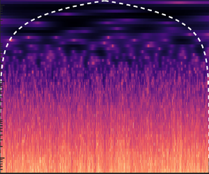
 As an example, figure 1 shows a set of one hour multifield time series and their wavelet PSDs. It is clear that multifield wavelet PSDs display branching structures of different intensities. More precisely, when  $\tau \gtrsim 10^2$ s, wavelet PSDs seem uniformly distributed in time, indicating that large-scale structures are time filling. As scale $\tau$ decreases, however, such large-scale structures divide asymmetrically and continuously into smaller structures, and thus the small-scale events appear to be increasingly spare.
Wavelet PSDs computed from the one hour dust storm dataset D1. (a,b) The one hour streamwise wind velocity time series ( $u$) and its local wavelet PSD $P_{u}$. (c,d) Same as (a,b) but for PM10 dust concentration $c10$. (e,f) Same as (a,b) but for wall-normal electric field $ez$. In panels (b,d,f), the regions enclosed by dashed lines and axes represent the ‘cone of influence’, where edge effects become important (Torrence & Compo Reference Torrence and Compo1998).

To evaluate the multifield increments in dust storms, we use a real-valued Morlet wavelet  $\psi _0(t)={\rm \pi} ^{-1/4} {\rm e}^{-t^2/2}\cos (6t)$ hereafter, as done in previous studies (e.g. Bacry et al. Reference Bacry, Arneodo, Frisch, Gagne and Hopfinger1991; Alexandrova et al. Reference Alexandrova, Carbone, Veltri and Sorriso-Valvo2008; Dupont et al. Reference Dupont, Argoul, Gerasimova-Chechkina, Irvine and Arneodo2020). As mentioned previously, the p.d.f.s of the field increments are a quantitative measure of the small-scale intermittency. It is widely accepted that the field difference $\Delta x(n',\tau )$ at time index $n'$ with increment $\tau$ for time series $x_n$ is proportional to the wavelet coefficient $W_x(n',\tau )$ (Farge Reference Farge1992; Farge et al. Reference Farge, Kevlahan, Perrier and Goirand1996; Camussi & Guj Reference Camussi and Guj1997; Salem et al. Reference Salem, Mangeney, Bale and Veltri2009). Thus, we obtain
 \begin{equation} \Delta x(n', \tau)=x(n')-x(n'+\tau) \sim W_x(n', \tau). \end{equation}
According to (2.5), the p.d.f. of the field increment  $\Delta x(n', \tau )$ can be replaced by that of the wavelet coefficient $W_x(n', \tau )$. The deviation of the p.d.f. of $W_x(n', \tau )$ from Gaussian is therefore a measure of the intermittency of the time series $x_n$ (Alexandrova et al. Reference Alexandrova, Carbone, Veltri and Sorriso-Valvo2008; Meyrand, Kiyani & Galtier Reference Meyrand, Kiyani and Galtier2015). In general, wavelet coefficients are normalized by their standard deviation at scale $\tau$, i.e. $W_x^\ast (n', \tau )=W_x(n', \tau ) /\langle W_x(n', \tau )^2\rangle ^{1/2}$. Accordingly, the probability distribution of $W_x^\ast (n', \tau )$ at different scales collapses onto a single p.d.f. if the time series $x_n$ satisfies scale invariance (i.e. self-similarity).
To quantify how the p.d.f. of the field increment  $\Delta x(n', \tau )$ deviates from Gaussian at various scales, the wavelet kurtosis can be defined as (Meneveau Reference Meneveau1991; Camussi & Guj Reference Camussi and Guj1997; Alexandrova et al. Reference Alexandrova, Carbone, Veltri and Sorriso-Valvo2008)
 \begin{equation} K_x(\tau)=\frac{\langle W_x(n', \tau)^4\rangle}{\langle W_x(n', \tau)^2\rangle^2}. \end{equation}
It is clear that  $K_x(\tau )$ is a measure of the tailedness (i.e. how often extreme events occur) of the p.d.f. of the field increment $\Delta x(n', \tau )$ at scale $\tau$. Since the kurtosis of a Gaussian p.d.f. is equal to 3, p.d.f.s with $K_x(\tau )>3$ exhibit long tails that exceed Gaussian characteristics (i.e. with high probabilities of extreme events). In contrast, p.d.f.s with $K_x(\tau )<3$ exhibit tails that are lower than those of Gaussian p.d.f.s (Frisch & Kolmogorov Reference Frisch and Kolmogorov1995; Bruno et al. Reference Bruno, Carbone, Sorriso-Valvo and Bavassano2003; Alexandrova et al. Reference Alexandrova, Carbone, Veltri and Sorriso-Valvo2008).
In addition to the non-Gaussian p.d.f.s of the field increments, anomalous scaling of the structure function is also a measure of small-scale intermittency (Frisch & Kolmogorov Reference Frisch and Kolmogorov1995; Sreenivasan & Antonia Reference Sreenivasan and Antonia1997; Dupont et al. Reference Dupont, Argoul, Gerasimova-Chechkina, Irvine and Arneodo2020). Within the inertial range, the  $p$th-order structure function of the time series $x_n, S_x^p(\tau )$, follows a power-law scaling:
 \begin{equation} S_x^p(\tau)=\langle|\Delta x(n', \tau)|^p\rangle \propto \tau^{\zeta(p)}, \end{equation}
where  $\zeta (p)$ is the scaling exponent. In the absence of intermittency (i.e. satisfying scale invariance or self-similarity), we can obtain $\zeta (p) \equiv p/3$, while $\zeta (p)< p/3$ is obtained in the presence of intermittency. In practice, to calculate the scaling exponent more conveniently and accurately, the scaling relationship in the form of extended self-similarity (ESS) can be used instead of (2.7) (Benzi et al. Reference Benzi, Ciliberto, Tripiccione, Baudet, Massaioli and Succi1993; Camussi & Guj Reference Camussi and Guj1997), which can be expressed as
 \begin{equation} \langle|\Delta x(n', \tau)|^p\rangle \sim\langle|\Delta x(n', \tau)|^3\rangle^{\zeta(p)}. \end{equation}
The main advantage of using (2.8) is that it exhibits a widely extended scaling range, even for low-Reynolds-number flows. Combining (2.5) and (2.8), the scaling relationship in the form of ESS can be rewritten as
 \begin{equation} \langle|W_x(n', \tau)|^p\rangle \propto\langle|W_x(n', \tau)|^3\rangle^{\zeta(p)}. \end{equation}
Based on (2.9), we can determine the scaling exponent  $\zeta (p)$ by a linear fit in a log–log plot.
To further unveil the role of small-scale intermittency in the scaling properties of structure functions, wavelet conditioning statistics were introduced to exclude the coherent components of the time series  $x_n$. The basic principle is that coherent structures are not space filling and thus cause bursts of strong fluctuations in measured values when they pass through the measurement points. Therefore, the coherent components resulting from these locally coherent structures can be represented by a small number of large wavelet coefficients (Farge Reference Farge1992; Farge et al. Reference Farge, Kevlahan, Perrier and Goirand1996; Camussi & Guj Reference Camussi and Guj1997; Sreenivasan & Antonia Reference Sreenivasan and Antonia1997; Salem et al. Reference Salem, Mangeney, Bale and Veltri2009; Osman et al. Reference Osman, Matthaeus, Wan and Rappazzo2012; Matsushima, Nagata & Watanabe Reference Matsushima, Nagata and Watanabe2021). Specifically, the wavelet coefficients of modulus $|W_x(n',\tau )|$ larger than a certain threshold are considered to correspond to coherent components, while coefficients of modulus smaller than the threshold are expected to correspond to random, incoherent components. Consequently, the scaling exponent of the conditioned structure function with considering fractal or no coherent components, $\tilde {\zeta }_x(p)$, can be determined by removing the wavelet coefficients of modulus larger than or equal to $F$ times their standard deviation:
 \begin{equation} |\widetilde{W_x}(n', \tau)|= \begin{cases}|W_x(n', \tau)| & \text{for} \ |W_x(n', \tau)|< F\langle W_x(n', \tau)^2\rangle^{1/2}, \\ 0 & \text{for} \ |W_x(n', \tau)| \geqslant F\langle W_x(n', \tau)^2\rangle^{1/2}, \end{cases} \end{equation}
where the constant  $F$ is termed conditioning factor. Obviously, the larger $F$ is, the larger the modulus of the coherent components removed from the time series $x_n$, and vice versa.
3. Results and discussion
3.1. The p.d.f.s of the field increments and wavelet kurtosis
Before proceeding with the data analysis, the convergence of high-order moments of multifield increments need to be examined. An example of the premultiplied p.d.f.s of multifield increments in the inertial ranges are presented in figure 2. It is found that these premultiplied p.d.f.s up to sixth order display decreasing tails, suggesting a statistical convergence of the used datasets (Meneveau & Marusic Reference Meneveau and Marusic2013; Carter & Coletti Reference Carter and Coletti2017).
(a–c) Premultiplied p.d.f.s of normalized streamwise velocity increments for the clean-air (red lines) and dust storm (blue lines) datasets at a time increment of  $\approx 20\tau _\eta$ from second to sixth order, where $\Delta u^+=\Delta u/u_\tau$. (d–f) Same as (a–c) but for the increments of PM10 dust concentration (i.e. $x=c10$) at a time increment of $\approx 0.5\tau _{ez}^{IR}$. (g–i) Same as (d–f) but for the increments of the streamwise component of the electric field (i.e. $x=ex$). For clarity, curves are divided by an arbitrary factor $\xi _p$ and smoothed by a 15 % bandwidth moving filter.

To characterize the small-scale multifield intermittency in dust storms, we begin by examining the p.d.f.s of the increments of streamwise wind velocity, PM10 dust concentration and electric fields. Figure 3 shows the p.d.f.s of the multifield increments at three different time scales within the inertial ranges. For both clean-air and dust storm datasets, the p.d.f.s of  $\Delta u$ are very close to Gaussian (i.e. near Gaussian) at $\tau =1.20$ s (figure 3c), indicating that the wind velocity is less intermittent at this scale. This occurs because vortices of various scales affect $\Delta u$ randomly at larger scales. As expected, with decreasing scale $\tau$, the p.d.f.s of $\Delta u$ become increasingly spiked and stretched. In particular, for $\tau =0.05\ \mathrm {s}$ (figure 3a), the p.d.f.s of $\Delta u$ deviate significantly from the Gaussian distribution and exhibit heavy exponential tails (i.e. super-Gaussian) with considerably high occurrence probabilities of extreme events. These non-Gaussian p.d.f.s are direct evidence for the small-scale intermittency of the wind velocity during dust storms, which has been widely demonstrated and studied in hydrodynamic and magnetohydrodynamic turbulence (Castaing et al. Reference Castaing, Gagne and Hopfinger1990; Praskovsky & Oncley Reference Praskovsky and Oncley1994; Tabeling et al. Reference Tabeling, Zocchi, Belin, Maurer and Willaime1996; Sorriso-Valvo et al. Reference Sorriso-Valvo, Carbone, Veltri, Consolini and Bruno1999; Alexandrova et al. Reference Alexandrova, Carbone, Veltri and Sorriso-Valvo2008; Meyrand et al. Reference Meyrand, Kiyani and Galtier2015). Additionally, the p.d.f.s of the dust storm datasets exhibit noticeably fatter and broader tails compared with those of clean-air datasets at $\tau =0.05$ s, suggesting that wind velocity in dust storms become more intermittent at small scales.
(a–c) The p.d.f.s of the increment of the streamwise wind velocity  $\Delta u(\tau )$ for the clean-air (red lines) and dust storm (blue lines) datasets at time scales $\tau =0.05$ s, $\tau =0.23$ s and $\tau =1.20$ s (determined by the wavelet coefficients). The dashed lines denote the standard Gaussian distribution. (d–f) Same as (a–c) but for the increments of PM10 dust concentration $\Delta c10(\tau )$ at time scales $\tau =2.64$ s, $\tau =4.92$ s and $\tau =9.84$ s. (g–i) Same as (d–f) but for the increments of electric field component $\Delta x(\tau )$, with $x\in \{ex,ey,ez\}$. For clarity, the spanwise and wall-normal components of the electric fields are vertically shifted by one and two decades, respectively.

Furthermore, it should be emphasized that since the PM10 dust concentration and electric fields are recorded at a sampling frequency of 1 Hz, the minimum time scale to evaluate their field increments is approximately 2.64 s, which is of the same order in figure 3c. However, in contrast to the near-Gaussian p.d.f. of  $\Delta u(\tau )$ at $\tau =1.20$ s, the p.d.f.s of $\Delta c 10(\tau )$ and $\Delta x(\tau )$ with $x \in \{ex, ey, ez\}$ within the range of $\tau =2.64\unicode{x2013}9.84\ {\rm s}$ are consistently non-Gaussian, suggesting that the PM10 dust concentration and electric fields exhibit small-scale intermittency over a broader range. Also, with decreasing scale $\tau$, the p.d.f.s seem to be more heavily tailed but with a slight change. The p.d.f.s exhibit remarkable exponential tails over the entire range of $\tau =2.64$–9.84 s. Notably, concerning the streamwise wind velocity, PM10 dust concentration and electric fields, the p.d.f.s of the increments for the four clean-air or six dust storm datasets are very similar, suggesting that the intermittent behaviour remains approximately unchanged among these datasets. Therefore, in the remainder of this paper, the results are presented in the form of ${\rm mean} \pm {\rm standard}$ deviation (std).
To quantify the degree of intermittency, a comparison of the wavelet kurtosis of the streamwise wind velocity, PM10 dust concentration and electric fields is shown in figure 4. It is apparent that the wavelet kurtosis values for the clean-air and dust storm datasets display a common trend when  $\tau \gtrsim 0.1$ s. Specifically, the kurtosis is approximately $K_u \sim 3$ within the range of $\tau \sim 5\unicode{x2013}100\ {\rm s}$, suggesting that the p.d.f.s of $\Delta u(\tau )$ should be near Gaussian. In the range of $\tau \sim 0.1\unicode{x2013}5\ {\rm s}$, $K_u$ increases gradually with decreasing $\tau$, indicating that the tails of the p.d.f.s of $\Delta u(\tau )$ become increasingly heavier. By contrast, for $\tau \lesssim 0.1$ s, $K_u$ of the dust storm datasets increases more rapidly than that of clean-air datasets with decreasing $\tau$. For instance, $K_u\approx 14$ for the dust storm datasets while $K_u\approx 5.6$ for the clean-air datasets when $\tau \approx 0.05$ s, consistent with fatter p.d.f.s for the dust storm datasets in figure 3(a). Thus, we conclude that small-scale intermittency of the streamwise wind velocity at time increments less than $\sim$0.1 s is significantly enhanced by the presence of dust particles. Such enhancements in small-scale intermittency of the carrier fluids are previously predicted by the numerical simulations of particle-laden turbulent flows in the two-way inter-phase coupling regime (Horwitz et al. Reference Horwitz, Rahmani, Geraci, Banko and Mani2016; Battista et al. Reference Battista, Gualtieri, Mollicone and Casciola2018; Horwitz & Mani Reference Horwitz and Mani2020). It is important to note that dust concentration in dust storms decrease exponentially with height above the surface (Shao Reference Shao2008). This means that, even though particle mass loading ratio is as low as $O(10^{-4})$ at 5 m height, it can reach $O(1)$ close to the surface (Creyssels et al. Reference Creyssels, Dupont, El Moctar, Valance, Cantat, Jenkins, Pasini and Rasmussen2009). As a result, it is reasonable to expect that dust particles inject wind velocity fluctuations at small scales in the near-surface region, thereby leading to relatively intense (extreme) velocity gradient events (see e.g. Horwitz & Mani Reference Horwitz and Mani2020).
(a) Comparison of the wavelet kurtosis of the PM10 dust concentration with that of the streamwise wind velocity for the clean-air (coloured in black) and dust storm (coloured in red) datasets. (b–d) Comparison of the wavelet kurtosis of the streamwise, spanwise and wall-normal electric fields with that of the streamwise wind velocity. The horizontal dashed lines denote the kurtosis of the standard Gaussian distribution (i.e.  $K_x=3$). The lines denote the mean of the nine datasets, and the error bars indicate mean $\pm$ std.

Although the wavelet kurtosis of the PM10 dust concentration and electric fields exhibits similar trends to that of the streamwise wind velocity, there are substantial differences in their magnitudes. As shown in figure 4, the wavelet kurtoses  $K_{c10}$, $K_{ex}$, $K_{ey}$ and $K_{ez}$ are significantly larger than $K_u$ within the range of $\tau \sim 2.7$–100 s, indicating that the increment p.d.f.s of the PM10 dust concentration and electric fields are flatter than those of the wind velocity at the same scale. Moreover, the wavelet kurtosis of the three components of the electric fields is almost indistinguishable but slightly smaller than that of the PM10 dust concentration, i.e. $K_{c10}>K_{ex}$ $\approx$ $K_{ex}$ $\approx$ $K_{ez}$. This is probably because the electric fields are dependent on all-sized charged dust particles, and thus, charged particles of diameters larger than $10\ \mathrm {\mu } \mathrm {m}$ and with relatively few extreme events may reduce the wavelet kurtosis of the electric fields. Interestingly, a large bump is observed in the wavelet kurtosis around $\tau =30$ s for PM10 dust concentration and electric fields. Such a time scale corresponds to the large-scale or very-large-scale motions in the atmospheric surface layer (e.g. Hutchins et al. Reference Hutchins, Chauhan, Marusic, Monty and Klewicki2012; Wang & Zheng Reference Wang and Zheng2016), which are believed to induce large-scale dust emissions from the sandy surface (see Zhang, Hu & Zheng Reference Zhang, Hu and Zheng2018), and thus probably manifest rare, large field increments of dust concentration and electric fields at large scales.
3.2. Anomalous scaling of the structure functions
To reveal higher-order statistical properties, we then turn our attention to the relationships between the scaling exponent  $\zeta (p)$ of the structure function and the order $p$. As an example, figure 5 shows how the scaling exponents $\zeta (p)$ for datasets C3 and D4 are determined by the ESS form (i.e. using (2.9)). When $p$ is small (e.g. $p=2$), there exists a good linear relationship between the wavelet coefficients $\langle |W(n', \tau )|^3\rangle$ and $\langle |W(n', \tau )|^p\rangle$ (e.g. $R^2$ varying from $\sim$0.98 to 1.0). However, the linearity between the wavelet coefficients decreases with increasing order $p$ because the measurement error is increasingly amplified. For instance, $R^2$ for the linear fitting of PM10 dust concentration is decreased to $\sim$0.78–0.94 when $p=6$. Therefore, this paper is limited to examining the structure functions of orders no more than 6. Figure 6 shows the scaling exponents $\zeta (p)$ as a function of the order within $p=6$. For lower orders $p<4$, it is found that the scaling exponents show excellent agreement with the Kolmogorov dimensional prediction, namely, $\zeta (p)=p / 3$. For higher orders $p \geqslant$ $4, \zeta (p)$ for all physical fields gradually deviates from the $\mathrm {K} 41$ theory with increasing $p$, revealing nonlinear dependence (i.e. anomalous scaling). This tendency of $\zeta (p)$ with $p$ indicates that all measured fields do not satisfy scale invariance (or self-similarity).
Scaling exponents  $\zeta (p)$ determined by the ESS form for (a) the streamwise wind velocity of the clean-air dataset C3 as well as (b) the streamwise wind velocity, (c) PM10 dust concentration, (d) streamwise electric field, (e) spanwise electric field and (f) wall-normal electric field for the dust storm dataset D4. The symbols indicate the measurements, and the dashed lines denote the linear fits in log–log coordinates (the slope is the scaling exponent).

Scaling exponents  $\zeta (p)$ as a function of order $p$ for (a) the streamwise wind velocity of the clean-air datasets, as well as (b) the streamwise wind velocity, (c) PM10 dust concentration, (d) streamwise electric field, (e) spanwise electric field and (f) wall-normal electric field of the dust storm datasets. The dashed lines denote the K41 theory (i.e. $\zeta (p)=p/3$), the error bars indicate the experimental measurements (i.e. mean $\pm$ std) and the solid lines represent the concatenate fitting results using (3.2) for all clean-air or dust storm datasets.

Having revealed the anomalous scaling for the multiple fields in dust storms, we next use the hierarchical structures theory of turbulence proposed by She and co-workers (hereafter referred to as the SL model) to fit an exact solution of the multifield anomalous scaling (e.g. She & Leveque Reference She and Leveque1994; She & Waymire Reference She and Waymire1995; She Reference She1998), providing additional physical insights into small-scale intermittency during dust storms, especially the most intermittent dissipative structures (Kritsuk et al. Reference Kritsuk, Norman, Padoan and Wagner2007; Meyrand et al. Reference Meyrand, Kiyani and Galtier2015). Briefly explained, Kolmogorov's refined similarity hypothesis argued that the turbulent energy dissipation rate  $\varepsilon _\tau$ is scale dependent rather than a constant (Kolmogorov Reference Kolmogorov1962), which yields the scaling $\langle \varepsilon _\tau ^p\rangle \propto \tau ^{\xi (p)}$ for the dissipation rate $\varepsilon _\tau ^p$. In addition, the first Kolmogorov refined hypothesis reads $\Delta u \propto (\varepsilon _\tau \tau )^{1/3}$, which leads to a relation between the scaling exponents of structure function and dissipation rate $\zeta (p)=p/3+\xi (p/3)$. Following the SL model, the dissipation rate of the log-Poisson distribution could yield the scaling exponent of the $p$th-order moment of the dissipation rate as (She & Leveque Reference She and Leveque1994; She & Waymire Reference She and Waymire1995; She Reference She1998)
 \begin{equation} \xi(p)={-}\lambda p+C(1-\beta^p), \end{equation}
where  $\lambda$ is the scaling exponent of the most intermittent dissipative structures or most singular structures; $C=d-D_{\infty }$ is the codimension of the space occupied by the most intermittent structures $(d=3$ is the spatial dimensionality and $D_{\infty }$ is the dimension of the most intermittent structure); and $\beta \in [0,1]$ is a parameter measuring the degree of intermittency. For $\beta =0$, this indicates the most intermittent state, and dissipation is concentrated in a singular structure; for $\beta =1$, this suggests no intermittency, consistent with the K41 theory (e.g. She Reference She1998; Meyrand et al. Reference Meyrand, Kiyani and Galtier2015). It is well known that the Kolmogorov 4/5 law, $\zeta (3)=1$, strictly holds within the inertial ranges (e.g. Kolmogorov Reference Kolmogorov1941; Pope Reference Pope2000; Xie & Bühler Reference Xie and Bühler2019), and thus $\lambda =C(1-\beta )$. Consequently, substituting this relationship into (3.1) and combining with the relation between the scaling exponents of structure function and dissipation rate gives
 \begin{equation} \zeta(p)=p/3-pC(1-\beta)/3+C(1-\beta^{p/3}). \end{equation}
It is worthwhile to note that, even though (3.2) was originally proposed for hydrodynamic turbulence, it has been successfully applied to other turbulent systems, such as magnetic fields in magnetohydrodynamic turbulence (e.g. Meyrand et al. Reference Meyrand, Kiyani and Galtier2015). We thus expect that the SL model could be reasonably extended to the PM10 dust concentration and electric fields in dust storms because these fields are closely related to the velocity field and exhibit a similar anomalous scaling.
The solid lines in figure 6 represent the concatenate fitting results for the nine datasets using (3.2), and the fitting parameters are summarized in table 2. The results show that the fitted curves of the SL model are in good agreement with the measurements (see  $R^2$ in table 2), suggesting that the behaviour of the multifield anomalous scaling in dust storms can be well described by the SL model. From table 2, we find that $\beta _u=0.685\pm 0.083$ in clean-air conditions, very close to the theoretical value $\beta =2/3$ suggested by She & Leveque (Reference She and Leveque1994) for the single-phase turbulent flows. However, we obtain $\beta _u= 0.628 \pm 0.079$ during dust storms, which is smaller than that in clean-air conditions, suggesting that the wind velocity fields during dust storms are more intermittent than those of single-phase turbulence, in accordance with figures 3(a) and 4(a). In particular, during dust storms, $\beta _u$ is found to be larger than $\beta _{c10}$, $\beta _{ex}$, $\beta _{ey}$ and $\beta _{ez}$, suggesting relatively weak intermittency for wind velocity. Specifically, among the multiple fields, $\beta _{c10}=0.469\pm 0.156$ is the smallest, further demonstrating that the PM10 dust concentration is more intermittent compared with the wind velocity and electric fields. With regard to the electric fields, it appears $\beta _{ez}>\beta _{ex} \sim \beta _{ey}$, indicating that the intermittency of the wall-normal electric field is relatively weak. However, this slight difference cannot be readily observed in the p.d.f.s of the field increments (figure 3) and wavelet kurtosis (figure 4).
Results of concatenate fitting of the clean-air and dust storm datasets using (3.2). The values are shown as the mean  $\pm$95 % confidence bounds. Here, $R^2$ is the coefficient of determination.

Moreover, the codimensions of the most intermittent structure of the wind velocity in clean-air and dust storms are  $C_u=2.090 \pm 0.536$ and $C_u=2.243 \pm 0.575$, respectively, which are very close to $C=2$ given in the single-phase turbulence (She & Leveque Reference She and Leveque1994). Meanwhile, we can obtain $D_{\infty,u}=3-C_u \sim 1$, suggesting that the most intermittent structure of the wind velocity during dust storms exhibits a nearly one-dimensional filamentary structure. This is consistent with the tube-like or highly intermittent filament vortex structures found in previous direct numerical simulations and experimental measurements of single-phase turbulence (e.g. Siggia Reference Siggia1981; She, Jackson & Orszag Reference She, Jackson and Orszag1990; Douady et al. Reference Douady, Couder and Brachet1991; Cadot, Douady & Couder Reference Cadot, Douady and Couder1995). In contrast, regarding PM10 dust concentration and electric fields, $C \sim 1$ and $D_{\infty } \sim 2$ can be obtained (see table 2), suggesting that their most intermittent structures tend to exhibit two-dimensional sheet structures. This is the same as the sheetlike structure of the passive conserved scalar in turbulent flows (Buch & Dahm Reference Buch and Dahm1996; Chen & Cao Reference Chen and Cao1997; Sreenivasan & Antonia Reference Sreenivasan and Antonia1997). The formation of such sheetlike structures for passive scalar is due to the fact that scalar gradients fluctuations tend to preferentially align with the direction of the most compressive strain rate, and thus scalar dissipation rate is concentrated in a thin layer (Ashurst et al. Reference Ashurst, Kerstein, Kerr and Gibson1987; Vedula, Yeung & Fox Reference Vedula, Yeung and Fox2001). During the observed dust storms, because the PM10 dust concentration at 5 m height is below ${\sim } 2\ {\rm mg}\ {\rm m}^{-3}$ (see table 1), corresponding to a particle mass loading ratio of $O(10^{-4})$. Therefore, the modulation of turbulence by dust particles is sufficiently weak at and above this height, and thus the PM10 dust concentration behaves in a similar behaviour as the passive scalar (see Celani et al. Reference Celani, Cencini, Mazzino and Vergassola2004). Moreover, since the electric fields are generated totally by charged dust particles, it is easy to foresee that the PM10 dust concentration and electric fields exhibit similar sheet structures. Notably, this two-dimensional sheet structure is considered to be more unstable than the one-dimensional filamentary structure (Chen & Cao Reference Chen and Cao1997).
3.3. Wavelet conditioning statistics
To uncover the role of small-scale intermittency in anomalous scaling, we determined how the scaling exponents of the conditioned structure functions vary with the conditioning factor. Figure 7 shows the scaling exponents of the conditioned structure functions of the wind velocity, PM10 dust concentration and electric fields for conditioning factors  $F=2$ and 15. As previously mentioned, the fraction of the removed wavelet coefficients increases with decreasing conditioning factor $F$. Since a large wavelet coefficient modulus corresponds to large gradients in the turbulent fields and can be considered to be associated with the presence of coherent structures, a small conditioning factor $F$ suggests that a large fraction of the coherent structures in the original fields is removed (Kiyani, Chapman & Hnat Reference Kiyani, Chapman and Hnat2006; Salem et al. Reference Salem, Mangeney, Bale and Veltri2009; Chowdhuri et al. Reference Chowdhuri, Iacobello and Banerjee2021). As shown in figure 7, with decreasing $F$, the deviation of the conditioned scaling exponents from the $\mathrm {K} 41$ theory gradually decreases for all observed physical quantities. In particular, for $F=2$, all conditioned scaling exponents are fairly consistent with the $\mathrm {K} 41$ theory (i.e. $\tilde {\zeta }_x(p) \approx p/3$, $x \in \{u, c, ex, ey, ez\}$). This indicates that when a sufficient fraction of the coherent structures is removed, the conditioned structure functions exhibit a well-defined Kolmogorov linear scaling and small-scale intermittency completely vanishes. Therefore, it is reasonable to infer that the small-scale intermittency (i.e. anomalous or multifractal scaling) of the multiple fields in dust storms is caused by the presence of small-scale coherent structures.
Conditioned scaling exponents  $\tilde {\zeta }(p)$ as a function of order $p$ for (a) the streamwise wind velocity of the clean-air datasets, as well as (b) the streamwise wind velocity, (c) PM10 dust concentration, (d) streamwise electric field, (e) spanwise electric field and (f) wall-normal electric field of the dust storm datasets at conditioning factors $F = 2$ and 15. The black dashed lines denote the K41 theory (i.e. $\zeta (p)=p/3$).

Furthermore, owing to the difference in the degree of multifield intermittency, the threshold conditioning factors above which  $\mathrm {K} 41$ linear scaling is recovered should vary from field to field. To further clarify this issue, the scaling exponents of the fifth- and sixth-order structure functions as a function of the conditioning factor are shown in figure 8. It can be seen that all scaling exponents appear a similar pattern. When $F$ is large, the conditioned scaling exponents are equal to those of the unconditioned structure functions and thus significantly deviate from the K41 theory, i.e. $\tilde {\zeta }(p)= \zeta (p)< p / 3$. This is because in such cases, there are no coherent components to be removed. When $F$ is decreased to the threshold value $F_{th2}$, the coherent structures start to be removed, and a further decrease in $F$ can lead to $\tilde {\zeta }(p)$ approaching the K41 theory. When $F$ is reduced to the threshold value $F_{thl}$, the coherent structures are completely removed. Hence, $\mathrm {K} 41$ scaling is recovered, i.e. $\tilde {\zeta }(p) \approx p / 3$. However, there are obvious differences in the threshold conditioning factors for the different physical fields, especially for $F_{th2}$, as indicated by the vertical dotted lines in figure 8. It can be seen that despite equal $F_{th1}$, $F_{th2}$ of the wind velocity in dust storms is much larger than that in clean-air conditions, further verifying a relatively strong intermittency in dust storms. Additionally, even though it is found that $F_{th1} \approx 1.0-1.5$ for all physical fields during dust storms, $F_{th2} \approx 15.5$ for the wind velocity, $F_{th2} \approx 14.0$ for the PM10 dust concentration and $F_{th2} \approx 11.0$–11.5 for the electric fields can be obtained. The reason for this is that the wind velocity is sampled at $50\ \mathrm {Hz}$, and thus, much finer velocity structures can be observed. Since the PM10 dust concentration and electric fields are sampled at the same frequency of 1 Hz, the PM10 dust concentration with a larger threshold interval (i.e. $F_{th2}-F_{th1}$) again demonstrates that its intermittency is stronger than that of the electric fields.
Conditioned scaling exponents  $\tilde {\zeta }(p)$ as a function of the conditioning factor $F$ at $p=5$ and 6 for (a) the streamwise wind velocity of the clean-air datasets, as well as (b) the streamwise wind velocity, (c) PM10 dust concentration, (d) streamwise electric field, (e) spanwise electric field and (f) wall-normal electric field of the dust storm datasets. The horizontal dashed lines indicate the K41 theory (i.e. $\zeta (p)=p/3$). The vertical dotted lines denote the threshold conditioning factors $F_{th1}$ and $F_{th2}$.

4. Conclusions
Dust storms represent a unique kind of dispersed electrohydrodynamic turbulence regime whose intermittency behaviour remains largely unknown. In this paper, using datasets obtained from the field measurements at the QLOA and a wavelet-based data analysis technique, we investigated the small-scale intermittency of the wind velocity, PM10 dust concentration and electric fields in dust storms for the first time. Notably, due to the limitation in the measurement techniques, only PM10 dust particles have been measured in our field observations and the coarser particles occupying over 90 % of the mass fraction are currently unable to be recorded. However, because electric fields in dust storms are produced by the total suspended charged particles, the inclusion of the analysis of electric fields can provide additional information about the unmeasured coarser particles to some extent. Overall, the key findings are threefold:
(i) During dust storms, the p.d.f.s of the increments of the multiple fields, which are evaluated by the wavelet coefficients, are found to deviate increasingly from Gaussian and exhibited extended exponential tails as scale $\tau$ decreases. The wavelet kurtosis substantially differed among the different fields, with the largest factor for the PM10 dust concentration and the smallest factor for the wind velocity. These results suggested that among the multiple fields in dust storms, the intermittency of the PM10 dust concentration is the strongest, while that of the wind velocity is the weakest. A relatively weak intermittency of electric fields compared with PM10 dust concentrations can be explained by considering the contribution of the coarser charged dust particles that are less intermittent due to large inertia (Battista et al. Reference Battista, Gualtieri, Mollicone and Casciola2018). Furthermore, a large bump is observed in the kurtosis of the PM10 dust concentrations and electric fields at large scale $\tau \sim 30$ s, which is probably caused by the large-scale dust emissions resulting from large- or very-large-scale motions in the atmospheric surface layer (Zhang et al. Reference Zhang, Hu and Zheng2018). More importantly, at $\tau \lesssim 0.1$ s, the increment p.d.f.s of the streamwise wind velocity in dust storms are broader and fatter than that in the clean-air conditions, and the kurtosis is significantly higher in dust storms. Such a difference in these p.d.f. and kurtosis implies that wind velocity at small scales becomes more intermittent in dust storms compared with the clean-air conditions. This phenomenon can be physically explained by the fact that dust particles of large mass loadings in the near-surface region inject velocity fluctuations at small scales and thus enhance the extreme velocity gradient events (Horwitz & Mani Reference Horwitz and Mani2020).
(ii) The scaling exponents of the multifield structure functions are expected to appear an anomalous scaling instead of Kolmogorov linear scaling. To gain a fundamental understanding of the underlying physics, the She–Leveque intermittency model (She & Leveque Reference She and Leveque1994) is used to fit exact solutions of the multifield anomalous scaling. It was determined that the measure of the intermittency degree is
$\beta _u=0.628 \pm 0.079$ in dust storms and $\beta _u=0.685 \pm 0.083$ in clean-air conditions, further verifying that the velocity field in dust storms is more intermittent than that in clean-air conditions. Also, we found the relationship $\beta _{c10}< \beta _{ex} \sim \beta _{ey}<\beta _{ez}<\beta _u$, again demonstrating that the small-scale intermittency of the PM10 dust concentration (wind velocity) is stronger (weaker) than that of the electric fields. Additionally, the dimension of the most intermittent structure is $D_{\infty } \sim 1$ for the wind velocity and $D_{\infty } \sim 2$ for the PM10 dust concentration and electric fields. These predictions suggest that the wind velocity exhibits a one-dimensional filamentary structure, while the PM10 dust concentration and electric fields exhibit two-dimensional sheet-like structures. The formation of these sheet-like structures in dust storms can be interpreted by the weak two-way couplings between the wind velocity and PM10 dust concentration at and above 5 m height. In such a case, PM10 dust concentration behave similarly to a passive scalar (Celani et al. Reference Celani, Cencini, Mazzino and Vergassola2004).(iii) On the basis of wavelet conditioning statistics, we found that Kolmogorov linear scaling was recovered for the multiple fields when the intermittent components were sufficiently removed from the raw data. We thus infer that the small-scale multifield intermittency in dust storms is actually attributed to the presence of small-scale coherent structures. In addition, the intervals between the two threshold conditioning factors seem to be quite different and are related to the sampling frequency and degree of small-scale intermittency.


Funding
This work was supported by the National Natural Science Foundation of China (grant number 92052202) and the Fundamental Research Funds for the Central Universities (grant number lzujbky-2021-ey19).
Declaration of interests
The authors report no conflict of interests.


