


1 Introduction
There has been an increasing emphasis in educational assessment on formative evaluation and diagnostic feedback (Black & Wiliam, Reference Black and Wiliam2009; Morris et al., Reference Morris, Perry and Wardle2021). Cognitive diagnostic assessment (CDA) addresses this need by providing detailed information about examinees’ mastery of specific skills or attributes (Leighton & Gierl, Reference Leighton and Gierl2007; Rupp et al., Reference Rupp, Templin and Henson2010). To improve the efficiency of CDA administration, cognitive diagnostic computerized adaptive testing (CD-CAT) has emerged as a powerful approach that combines the benefits of cognitive diagnosis with the efficiency of adaptive testing (Cheng, Reference Cheng2009).
A critical component in CD-CAT is the item selection algorithm, which determines the items and the sequence in which they are administered to each examinee. Various item selection methods have been proposed, most of which are fundamentally connected through information theory principles, as demonstrated by Cheng (Reference Cheng2009) and Wang et al. (Reference Wang, Song, Wang, Gao and Xiong2020). These methods include the original Kullback–Leibler (KL) index (Xu et al., Reference Xu, Chang and Douglas2003), likelihood-weighted KL and posterior-weighted KL (PWKL) indices (Cheng, Reference Cheng2009), modified PWKL (MPWKL) index (Kaplan et al., Reference Kaplan, De La Torre and Barrada2015), the Shannon entropy (SHE) procedure (Tatsuoka, Reference Tatsuoka2002), and mutual information methods (Wang, Reference Wang2013). While these approaches may appear distinct, they all derive from related information-theoretic concepts, with KL divergence, Shannon entropy, and mutual information sharing deep mathematical connections in quantifying information gain and uncertainty reduction (Cover & Thomas, Reference Cover and Thomas1991). More recently, the generalized deterministic inputs, noisy “and” gate (G-DINA) model discrimination index (GDI) was introduced as an efficient alternative (Kaplan et al., Reference Kaplan, De La Torre and Barrada2015). GDI quantifies the weighted variance in item success probabilities given a specific attribute distribution.
While these methods have demonstrated effectiveness in attribute-level classification accuracy, they face a significant computational challenge: as the number of attributes (K) increases, the computational burden grows exponentially. This occurs because most existing methods require evaluating all possible attribute patterns ( ${2}^K$
) for each item in the bank before selecting the most suitable one as the next item to administer. For instance, with K = 10 attributes, algorithms must evaluate 1,024 possible patterns for each candidate item. This computational intensity can make real-time implementation challenging, particularly in settings requiring rapid item selection decisions.
${2}^K$
) for each item in the bank before selecting the most suitable one as the next item to administer. For instance, with K = 10 attributes, algorithms must evaluate 1,024 possible patterns for each candidate item. This computational intensity can make real-time implementation challenging, particularly in settings requiring rapid item selection decisions.
The only existing method that attempts to reduce the computational burden is the GDI method, which partially addresses this issue by working with reduced attribute patterns. Although GDI is more computationally efficient than the PWKL method (Kaplan et al., Reference Kaplan, De La Torre and Barrada2015), which is known to be the most computationally intensive, its efficiency relative to KL and SHE—two other widely discussed methods in CD-CAT—remains unclear. This study aims to address this gap by evaluating GDI’s computational efficiency relative to KL and SHE. Moreover, the primary objective is to propose a novel and flexible approach that not only substantially reduces computational demands but also maintains the theoretical foundations and measurement precision of existing methods.
This article introduces the likelihood-based profile shrinkage (LBPS) algorithm as a solution to this challenge. The key insight of LBPS is that as testing proceeds, the set of plausible attribute patterns for an examinee rapidly shrinks based on their response patterns. By focusing only on the most likely attribute patterns, LBPS achieves substantial efficiency gains while preserving measurement accuracy. Importantly, LBPS can be integrated with any existing item selection method, making it a flexible enhancement to current CD-CAT implementations. In addition, LBPS can be implemented without requiring changes to existing item banks or cognitive diagnostic models (CDMs). Through simulation studies, we demonstrate that LBPS achieves comparable attribute classification accuracy to traditional methods while greatly reducing computation time, particularly for long tests measuring larger numbers of attributes. The remainder of this article is organized as follows. Section 2 reviews the theoretical framework of CDMs and existing item selection methods. Section 3 introduces the LBPS algorithm and establishes its theoretical properties. Section 4 presents simulation studies comparing LBPS with existing methods across various conditions. Section 5 discusses practical implications and future research directions.
2 Background
2.1 CDM framework
2.1.1 Basic setup
CDMs aim to provide detailed information about examinees’ mastery of specific skills or attributes underlying test performance. In CDA, the goal is to measure examinees’ mastery of K discrete attributes or skills. Each examinee’s mastery profile is represented by an attribute pattern $\boldsymbol{\alpha} =\left({\alpha}_1,\dots, {\alpha}_K\right)$
where
$\boldsymbol{\alpha} =\left({\alpha}_1,\dots, {\alpha}_K\right)$
where ${\alpha}_k=1$
indicates mastery of attribute k and
${\alpha}_k=1$
indicates mastery of attribute k and ${\alpha}_k=0$
indicates non-mastery for k = 1, 2, …, K attributes. Note that the terms “pattern” and “profile” are used interchangeably in the paper to refer to α. For K attributes, there are
${\alpha}_k=0$
indicates non-mastery for k = 1, 2, …, K attributes. Note that the terms “pattern” and “profile” are used interchangeably in the paper to refer to α. For K attributes, there are ${2}^K$
possible attribute patterns, representing all possible combinations of mastery and non-mastery across the measured attributes (de la Torre, Reference de la Torre2011). The relationship between items and attributes is specified through a J × K Q-matrix (Tatsuoka, Reference Tatsuoka, Nichols, Chipman and Brennan1995), where entry
${2}^K$
possible attribute patterns, representing all possible combinations of mastery and non-mastery across the measured attributes (de la Torre, Reference de la Torre2011). The relationship between items and attributes is specified through a J × K Q-matrix (Tatsuoka, Reference Tatsuoka, Nichols, Chipman and Brennan1995), where entry ${q}_{jk}=1$
if item j requires attribute k and
${q}_{jk}=1$
if item j requires attribute k and ${q}_{jk}=0$
otherwise. The Q-matrix represents the cognitive specifications of the test by mapping each item to its required attributes.
${q}_{jk}=0$
otherwise. The Q-matrix represents the cognitive specifications of the test by mapping each item to its required attributes.
2.1.2 Types of CDMs
CDMs can be categorized based on how they model the relationship between attributes and item responses (Ravand & Baghaei, Reference Ravand and Baghaei2020). In conjunctive models, examinees must master all required attributes to have a high probability of correctly answering an item. The Deterministic Inputs, Noisy “And” Gate (DINA) model (Junker & Sijtsma, Reference Junker and Sijtsma2001) and the Noisy Inputs, Deterministic “And” Gate (NIDA) model (Maris, Reference Maris1999) are prominent examples of conjunctive models. These models are particularly appropriate when skills build upon each other in a non-compensatory way. Disjunctive models assume that mastery of any one of the required attributes is sufficient for a high probability of success. The Deterministic Input, Noisy “Or” Gate (DINO) model (Templin & Henson, Reference Templin and Henson2006) exemplifies this approach. Such models are suitable when multiple solution strategies can lead to correct answers and mastery of one attribute can compensate for non-mastery of others.
Additive models, such as the additive CDM (ACDM; de la Torre, Reference de la Torre2011) and the linear logistic model (LLM; Maris, Reference Maris1999), take a different approach in which each mastered attribute contributes independently to the probability of a correct response. These models are appropriate when attributes have cumulative but independent effects on performance.
More recently, general diagnostic models have been developed that can accommodate multiple types of attribute relationships within the same assessment. The generalized DINA model (G-DINA; de la Torre, Reference de la Torre2011), the log-linear CDM (LCDM; Henson et al., Reference Henson, Templin and Willse2009), and the general diagnostic model (GDM; von Davier, Reference von Davier2005) allow different items to exhibit different attribute relationships. These general models provide greater flexibility but typically require larger sample sizes for stable parameter estimation.
2.1.3 The DINA model
While the methods developed in this article apply to any CDM, we use the DINA model for illustration due to its parsimony and wide use in diagnostic testing applications (Junker & Sijtsma, Reference Junker and Sijtsma2001; de la Torre, Reference de la Torre2009). Under the DINA model, an examinee must master all required attributes to have a high probability of answering an item correctly, making it a conjunctive model. For an examinee i with attribute pattern α responding to item j, the ideal response is
 $$\begin{align}{\eta}_{ij}\left(\boldsymbol{\alpha} \right)=\prod \limits_{k=1}^K{\alpha_{ik}}^{q_{jk}},\end{align}$$
where ${\eta}_{ij}\left(\boldsymbol{\alpha} \right)=1$
indicates mastery of all required attributes and
${\eta}_{ij}\left(\boldsymbol{\alpha} \right)=1$
indicates mastery of all required attributes and ${\eta}_{ij}\left(\boldsymbol{\alpha} \right)=0$
indicates a lack of at least one required attribute (de la Torre, Reference de la Torre2009).
${\eta}_{ij}\left(\boldsymbol{\alpha} \right)=0$
indicates a lack of at least one required attribute (de la Torre, Reference de la Torre2009).
The probability of a correct response of examinee i on item j is given by
 $$\begin{align}P\left({X}_{ij}=1|\boldsymbol{\alpha} \right)={\left(1-{s}_j\right)}^{\eta_{ij}\left(\boldsymbol{\alpha} \right)}{g_j}^{1-{\eta}_{ij}\left(\boldsymbol{\alpha} \right)},\end{align}$$
where ${s}_j$
is the slipping parameter (probability of incorrect response despite mastery) and
${s}_j$
is the slipping parameter (probability of incorrect response despite mastery) and ${g}_j$
is the guessing parameter (probability of correct response despite non-mastery). These item parameters account for the probabilistic nature of the response process, where examinees who have mastered all required attributes may still make mistakes (slips), and those who lack required attributes may still answer correctly through guessing (de la Torre & Douglas, Reference de la Torre and Douglas2004). The DINA model’s simple form makes it particularly useful for understanding the fundamental principles of cognitive diagnosis while still capturing essential features of the response process. Its parsimony in parameter estimation and clear interpretation of results have made it a popular choice in diagnostic testing applications.
${g}_j$
is the guessing parameter (probability of correct response despite non-mastery). These item parameters account for the probabilistic nature of the response process, where examinees who have mastered all required attributes may still make mistakes (slips), and those who lack required attributes may still answer correctly through guessing (de la Torre & Douglas, Reference de la Torre and Douglas2004). The DINA model’s simple form makes it particularly useful for understanding the fundamental principles of cognitive diagnosis while still capturing essential features of the response process. Its parsimony in parameter estimation and clear interpretation of results have made it a popular choice in diagnostic testing applications.
2.2 Item selection methods in CD-CAT
Item selection methods in CD-CAT can be broadly categorized into parametric and nonparametric approaches (Chang et al., Reference Chang, Chiu and Tsai2019). While non-parametric methods have emerged recently to address certain limitations of parametric approaches (Chiu & Chang, Reference Chiu and Chang2021), parametric methods remain fundamental to CD-CAT implementation. These parametric methods can be further classified as single-purpose or dual-purpose (Wang et al., Reference Wang, Chang and Douglas2012). Single-purpose methods focus solely on optimizing the measurement of attribute profiles, while dual-purpose methods simultaneously measure both attribute profiles and general ability (Dai et al., Reference Dai, Zhang and Li2016; Kang et al., Reference Kang, Zhang and Chang2017; Wang et al., Reference Wang, Zheng and Chang2014). This article proposes a new algorithm within the framework of parametric single-purpose item selection methods. Therefore, we focus our review on existing methods in this category, which form the foundation for CD-CAT item selection and remain the most widely used in practice.
2.2.1 Basic framework
In CD-CAT, parametric single-purpose item selection methods aim to optimize the measurement of examinees’ attribute mastery profiles. These methods utilize item parameters and probability models within a cognitive diagnostic framework to select items that maximize information about attribute patterns. After J items have been administered to an examinee, let ${\boldsymbol{x}}_{\boldsymbol{J}}=\left({x}_1,\dots, {x}_J\right)$
denote the vector of observed responses, where xj
∈ {0,1}. Following Bayes’ theorem, the posterior probability of the attribute pattern is
${\boldsymbol{x}}_{\boldsymbol{J}}=\left({x}_1,\dots, {x}_J\right)$
denote the vector of observed responses, where xj
∈ {0,1}. Following Bayes’ theorem, the posterior probability of the attribute pattern is
 $$\begin{align}\pi \left(\boldsymbol{\alpha} |{\boldsymbol{x}}_{\boldsymbol{J}}\right)\propto {\pi}_0\left(\boldsymbol{\alpha} \right)L\left({\boldsymbol{x}}_{\boldsymbol{J}}|\boldsymbol{\alpha} \right),\end{align}$$
where ${\pi}_0\left(\boldsymbol{\alpha} \right)$
is the prior probability and
${\pi}_0\left(\boldsymbol{\alpha} \right)$
is the prior probability and $L\left({\boldsymbol{x}}_{\boldsymbol{J}}|\boldsymbol{\alpha} \right)={\prod}_{j=1}^JP\left({X}_j={x}_j|\boldsymbol{\alpha} \right)$
is the likelihood function under the specified CDM. Define the item h as a candidate item in the pool of available items, from which the (J+1)-th item is to be selected based on a specified item selection method.
$L\left({\boldsymbol{x}}_{\boldsymbol{J}}|\boldsymbol{\alpha} \right)={\prod}_{j=1}^JP\left({X}_j={x}_j|\boldsymbol{\alpha} \right)$
is the likelihood function under the specified CDM. Define the item h as a candidate item in the pool of available items, from which the (J+1)-th item is to be selected based on a specified item selection method.
2.2.2 Information-theoretic methods.
Kullback–Leibler-based approaches
The Kullback–Leibler (KL) information (Cover & Thomas, Reference Cover and Thomas1991; Kullback & Leibler, Reference Kullback and Leibler1951) provides a foundation for measuring the distance between probability distributions under different attribute patterns. For item j and two attribute patterns $\boldsymbol{\alpha}, \boldsymbol{\alpha}^{\prime}\in {\left\{0,1\right\}}^K$
, the KL information is defined as
$\boldsymbol{\alpha}, \boldsymbol{\alpha}^{\prime}\in {\left\{0,1\right\}}^K$
, the KL information is defined as
 $$\begin{align}D_j\!\left(\boldsymbol{\alpha} \,\|\, \boldsymbol{\alpha}'\right)&=\sum_{x=0}^1P\left({X}_j=x|\boldsymbol{\alpha} \right){log}\;\left[\frac{P\left({X}_j=x|\boldsymbol{\alpha} \right)}{P\left({X}_j=x|{\boldsymbol{\alpha}}^{\prime}\right)}\right],\end{align}$$
where $P\left({X}_j=x|\boldsymbol{\alpha} \right)$
denotes the probability of response x given attribute pattern
$P\left({X}_j=x|\boldsymbol{\alpha} \right)$
denotes the probability of response x given attribute pattern $\boldsymbol{\alpha}$
under the specified CDM. Building on this framework, the KL index was proposed by Xu et al. (Reference Xu, Chang and Douglas2003) to select the next item maximizing:
$\boldsymbol{\alpha}$
under the specified CDM. Building on this framework, the KL index was proposed by Xu et al. (Reference Xu, Chang and Douglas2003) to select the next item maximizing:
 $$\begin{align}KL_h\left(\widehat{\boldsymbol{\alpha}}\right)=\sum_{c=1}^{2^K}D_h\!\left(\widehat{\boldsymbol{\alpha}} \,\|\, \boldsymbol{\alpha}_c\right),\end{align}$$
where h represents the candidate item in the pool of available items, $\widehat{\boldsymbol{\alpha}}$
is the current estimate of the examinee’s attribute pattern, and c indexes attribute patterns (c = 1, 2, …,
$\widehat{\boldsymbol{\alpha}}$
is the current estimate of the examinee’s attribute pattern, and c indexes attribute patterns (c = 1, 2, …, ${2}^K$
). This index measures the total divergence between the response distributions under the estimated pattern and all other possible patterns. Cheng (Reference Cheng2009) enhanced this approach by incorporating posterior probabilities through the posterior-weighted KL (PWKL) index:
${2}^K$
). This index measures the total divergence between the response distributions under the estimated pattern and all other possible patterns. Cheng (Reference Cheng2009) enhanced this approach by incorporating posterior probabilities through the posterior-weighted KL (PWKL) index:
 $$\begin{align}PWKL_h\!\left(\widehat{\boldsymbol{\alpha}}\right)&=\sum_{c=1}^{2^K}D_h\!\left(\widehat{\boldsymbol{\alpha}} \,\|\, \boldsymbol{\alpha}_c\right)\pi\!\left(\boldsymbol{\alpha}_c|\boldsymbol{x}_J\right),\end{align}$$
where $\pi \left({\boldsymbol{\alpha}}_c|{\boldsymbol{x}}_J\right)$
is the posterior probability after J items have been answered, and
$\pi \left({\boldsymbol{\alpha}}_c|{\boldsymbol{x}}_J\right)$
is the posterior probability after J items have been answered, and ${\boldsymbol{x}}_J$
is the response vector.
${\boldsymbol{x}}_J$
is the response vector.
Other KL information-based item selection methods include the modified PWKL (MPWKL) method (Kaplan et al., Reference Kaplan, De La Torre and Barrada2015), and posterior-weighted CDM discrimination index (PWCDI) method (Zheng & Chang, Reference Zheng and Chang2016). This study employs only PWKL for comparison, as MPWKL, while achieving comparable performance to GDI, incurs substantial computational costs (Kaplan et al., Reference Kaplan, De La Torre and Barrada2015). Additionally, PWCDI demonstrates inferior performance to PWKL with small calibration samples (Chang et al., Reference Chang, Chiu and Tsai2019), making PWKL the most suitable KL-based comparator for this investigation.
Shannon entropy-based approaches.
Shannon entropy (Cover & Thomas, Reference Cover and Thomas1991; Shannon, Reference Shannon1948) provides an alternative framework for quantifying uncertainty in the posterior distribution of attribute patterns. In the context of CD-CAT, after J items have been selected, the entropy of a distribution $\pi$
is defined as
$\pi$
is defined as
 $$\begin{align}H\left(\pi \right)=-\sum_{c=1}^{2^K}\pi \left({\boldsymbol{\alpha}}_c|{\boldsymbol{x}}_J\right){log}\;\left[\pi \left({\boldsymbol{\alpha}}_c|{\boldsymbol{x}}_J\right)\right].\end{align}$$
Lower entropy values indicate greater certainty about the true attribute pattern. Building on information theory principles (Cover & Thomas, Reference Cover and Thomas1991), Tatsuoka (Reference Tatsuoka2002) proposed selecting items by minimizing the expected posterior entropy:
 $$\begin{align}SH{E}_h=\sum_{x=0}^1H\left(\pi |{X}_h=x,{\boldsymbol{x}}_J\right)P\left({X}_h=x|{\boldsymbol{x}}_J\right),\end{align}$$
where $\pi \mid {X}_h=x,{\boldsymbol{x}}_{\boldsymbol{J}}$
denotes the posterior distribution after observing response x to the candidate item h in the pool of available items,
$\pi \mid {X}_h=x,{\boldsymbol{x}}_{\boldsymbol{J}}$
denotes the posterior distribution after observing response x to the candidate item h in the pool of available items, $P\left({X}_h=x|{\boldsymbol{x}}_{\boldsymbol{J}}\right)$
denotes the predicted probability of observing response x conditional on the response vector
$P\left({X}_h=x|{\boldsymbol{x}}_{\boldsymbol{J}}\right)$
denotes the predicted probability of observing response x conditional on the response vector ${\boldsymbol{x}}_J$
, and
${\boldsymbol{x}}_J$
, and
 $$\begin{align}P\left({X}_h=x|{\boldsymbol{x}}_J\right)=\sum_{c=1}^{2^K}P\left({X}_h=x|{\boldsymbol{\alpha}}_c\right)\pi \left({\boldsymbol{\alpha}}_c|{\boldsymbol{x}}_J\right).\end{align}$$
Recent methodological advances have extended this framework through the expected mutual information index (Wang, Reference Wang2013) and the Jensen–Shannon divergence (JSD) index (Minchen & de la Torre, Reference Minchen and de la Torre2016; Yigit et al., Reference Yigit, Sorrel and De La Torre2019). Theoretical investigations have established that JSD is mathematically equivalent to mutual information in quantifying the information gain about an examinee’s attribute pattern (Yigit et al., Reference Yigit, Sorrel and De La Torre2019). Furthermore, a linear relationship was found between SHE and JSD (Wang et al., Reference Wang, Song, Wang, Gao and Xiong2020), indicating that these methods yield equivalent item selection decisions in CD-CAT applications. Given these theoretical equivalences, the present study employs the SHE method (Tatsuoka, Reference Tatsuoka2002) as the representative entropy-based approach in our comparative analyses.
2.2.3 GDI approach
Building on the G-DINA framework (de la Torre, Reference de la Torre2011), Kaplan et al. (Reference Kaplan, De La Torre and Barrada2015) introduced the G-DINA discrimination index (GDI). This index offers computational advantages by working with reduced attribute patterns, which are made up by ${K}_h^{\ast }$
attributes required by item h. For example, if a
q
-vector is defined as (1, 0, 1, 0, 1),
${K}_h^{\ast }$
attributes required by item h. For example, if a
q
-vector is defined as (1, 0, 1, 0, 1), ${K}_h^{\ast }=3$
attributes since this item only requires the first, third, and fifth attributes. Consequently, there are eight reduced attribute patterns based on the three required attributes. The GDI for item h is defined as
${K}_h^{\ast }=3$
attributes since this item only requires the first, third, and fifth attributes. Consequently, there are eight reduced attribute patterns based on the three required attributes. The GDI for item h is defined as
 $$\begin{align}GD{I}_h=\sum_{c=1}^{2^{K_h^{\ast }}}\pi \left({\boldsymbol{\alpha}}_{ch}^{\ast}\right){\left[P\left({X}_h=1|\;{\boldsymbol{\alpha}}_{ch}^{\ast}\right)-{\overline{P}}_h\right]}^2,\end{align}$$
where ${\boldsymbol{\alpha}}_{ch}^{\ast }$
represents the c-th reduced attribute pattern for item h (
${\boldsymbol{\alpha}}_{ch}^{\ast }$
represents the c-th reduced attribute pattern for item h ( $c=1,2,\dots, {2}^{K_h^{\ast }}$
),
$c=1,2,\dots, {2}^{K_h^{\ast }}$
), $\pi \left({\boldsymbol{\alpha}}_{ch}^{\ast}\right)$
is the posterior probability of the reduced attribute pattern after J items have been selected, and
$\pi \left({\boldsymbol{\alpha}}_{ch}^{\ast}\right)$
is the posterior probability of the reduced attribute pattern after J items have been selected, and ${\overline{P}}_h=\sum_{c=1}^{2^{K_h^{\ast }}}\pi \left({\boldsymbol{\alpha}}_{ch}^{\ast}\right)P\left({X}_h=1|{\boldsymbol{\alpha}}_{ch}^{\ast}\right)$
is the mean success probability. The GDI measures an item’s ability to differentiate between reduced attribute vectors, emphasizing those with higher success probabilities. The item with the highest GDI in the pool is selected.
${\overline{P}}_h=\sum_{c=1}^{2^{K_h^{\ast }}}\pi \left({\boldsymbol{\alpha}}_{ch}^{\ast}\right)P\left({X}_h=1|{\boldsymbol{\alpha}}_{ch}^{\ast}\right)$
is the mean success probability. The GDI measures an item’s ability to differentiate between reduced attribute vectors, emphasizing those with higher success probabilities. The item with the highest GDI in the pool is selected.
2.2.4 Comparative properties
These methods offer distinct advantages for a single-purpose CD-CAT. The KL-based methods directly measure discrimination between attribute patterns, with PWKL improving upon the original KL index by incorporating posterior information (Cheng, Reference Cheng2009). The entropy-based methods approach item selection through uncertainty reduction in the posterior distribution. While SHE directly minimizes expected uncertainty, the mutual information method provides a theoretically equivalent formulation through information gain (Wang, Reference Wang2013). The GDI achieves computational efficiency through dimension reduction while maintaining measurement precision, particularly advantageous for assessments with many attributes (Kaplan et al., Reference Kaplan, De La Torre and Barrada2015). Despite their demonstrated effectiveness, opportunities remain for improving attribute pattern estimation efficiency in CD-CAT. The following section introduces a LBPS algorithm that builds upon these theoretical foundations while addressing certain limitations in existing approaches.
2.3 Computational considerations in CD-CAT
The practical implementation of CD-CAT item selection methods faces significant computational challenges, primarily arising from the need to evaluate large numbers of attribute patterns during the item selection process. For KL-based methods, item selection entails computing and summing up the KL information between the current attribute pattern estimate and all ${2}^K$
possible patterns, and this is done for all eligible items in the bank. When using PWKL, additional computational burden comes from calculating posterior probabilities for each pattern combination.
${2}^K$
possible patterns, and this is done for all eligible items in the bank. When using PWKL, additional computational burden comes from calculating posterior probabilities for each pattern combination.
Consider a test measuring K = 5 attributes with an item bank of 300 items as an example. Even in this relatively simple case, 32 possible attribute patterns must be evaluated for each item selection decision. The PWKL method requires computing and summing KL divergence values across all 32 patterns for each item under consideration. This computation must be performed for all eligible items in the bank to select the next item. The Shannon entropy method involves similar computational intensity, requiring the calculation of expected entropy by evaluating posterior distributions for possible responses across all attribute patterns, again repeated for each item in the bank.
The GDI method introduced by Kaplan et al. (Reference Kaplan, De La Torre and Barrada2015) offers some computational advantages by working only with the attributes required for each item. This reduces the pattern space from ${2}^K$
to
${2}^K$
to ${2}^{K_h^{\ast }}$
, where
${2}^{K_h^{\ast }}$
, where ${K}_h^{\ast}$
is typically much smaller than K, and requires fewer posterior probability calculations. However, even with these improvements, significant computational challenges remain. These computational demands become particularly acute when tests measure many attributes and as the item bank expands.
${K}_h^{\ast}$
is typically much smaller than K, and requires fewer posterior probability calculations. However, even with these improvements, significant computational challenges remain. These computational demands become particularly acute when tests measure many attributes and as the item bank expands.
The practical implications of these computational demands are substantial. They can affect response time between items, overall test administration efficiency, and the system resources required to implement CD-CAT. When multiple examinees are tested simultaneously, as is common in educational settings, these computational requirements become even more demanding. While the GDI method has made progress in reducing computational burden through reduced attribute patterns, there remains a clear need for more efficient approaches that can maintain measurement precision while reducing computation time and scaling effectively with the number of attributes.
3 The likelihood-based profile shrinkage algorithm
3.1 Key ideas
The computational burden of traditional CD-CAT item selection methods grows exponentially with the number of attributes K, as each method evaluates all ${2}^K$
possible attribute patterns for each eligible item in the bank at every item selection decision. However, as testing proceeds, the set of plausible, or most likely, attribute patterns for an examinee typically shrinks based on their response pattern. This observation motivates the key insight of LBPS: by focusing on the most likely attribute patterns for item selection while maintaining full pattern space for estimation, substantial computational savings can be achieved without sacrificing measurement precision.
${2}^K$
possible attribute patterns for each eligible item in the bank at every item selection decision. However, as testing proceeds, the set of plausible, or most likely, attribute patterns for an examinee typically shrinks based on their response pattern. This observation motivates the key insight of LBPS: by focusing on the most likely attribute patterns for item selection while maintaining full pattern space for estimation, substantial computational savings can be achieved without sacrificing measurement precision.
The likelihood function provides a natural mechanism for identifying these plausible patterns. After each response, patterns with maximum likelihood represent the most probable true states given the observed data. Figure 1 illustrates changes in attribute profiles’ likelihoods using LBPS with KL when K = 5. Early on, multiple profiles may have similar likelihoods, but as the test proceeds, the number of likely profiles shrinks (see Figure 1). By restricting item selection calculations to these patterns while using all patterns for estimation, LBPS balances computational efficiency with measurement accuracy.
An illustration of changes in attribute profiles’ likelihoods using LBPS with KL when K = 5.
Note: An iteration refers to a single cycle of the adaptive testing process: selecting the next item, collecting the examinee’s response, and updating the likelihoods of all attribute profiles and the examinee’s estimated attribute profile based on the accumulated responses.

Figure 1 Long description
Top-left panel, labeled After the First Iteration, shows the y-axis labeled Likelihood from 0 to 1 and the x-axis labeled Attribute Profiles from 0 to 32. Most likelihood values are either near 1 or near 0, with a few profiles at high likelihood. Top-right panel, After the Second Iteration, shows a similar pattern but with more attribute profiles at lower likelihoods and fewer at high likelihood. Bottom-left panel, After the Third Iteration, shows further concentration, with only a few profiles above 0.6 and the rest near zero. Bottom-right panel, After the Fourth Iteration, shows a single profile near 0.6 and all others close to zero. Across panels, the likelihood distribution becomes increasingly peaked, indicating that the adaptive process narrows the estimated attribute profile with each iteration.
3.2 Theoretical framework
Let ${\boldsymbol{x}}_t=\left({x}_1,\dots, {x}_t\right)$
denote the response vector after t items have been administered. For any attribute pattern
${\boldsymbol{x}}_t=\left({x}_1,\dots, {x}_t\right)$
denote the response vector after t items have been administered. For any attribute pattern $\boldsymbol{\alpha} \in A={\left\{0,1\right\}}^K$
, the likelihood under a cognitive diagnostic model is
$\boldsymbol{\alpha} \in A={\left\{0,1\right\}}^K$
, the likelihood under a cognitive diagnostic model is
 $$\begin{align}L\left(\boldsymbol{\alpha} |{\boldsymbol{x}}_t\right)=\prod \limits_{j=1}^tP\left({X}_j={x}_j|\boldsymbol{\alpha} \right).\end{align}$$
Define the set of attribute patterns with the largest likelihood after t items have been answered as
 $$\begin{align}M\left({\boldsymbol{x}}_t\right)=\arg \underset{\boldsymbol{\alpha} \in A}{\max }L\left(\boldsymbol{\alpha} |{\boldsymbol{x}}_t\right).\kern0.36em\end{align}$$
For the response pattern ${\boldsymbol{x}}_t$
and a new item j that is answered with a response
${\boldsymbol{x}}_t$
and a new item j that is answered with a response ${x}_j$
,
${x}_j$
, $L\left(\boldsymbol{\alpha} |{\boldsymbol{x}}_{\boldsymbol{t}},{x}_j\right)=L\left(\boldsymbol{\alpha} |{\boldsymbol{x}}_{\boldsymbol{t}}\right)P\left({X}_j={x}_j|\boldsymbol{\alpha} \right)$
.
$L\left(\boldsymbol{\alpha} |{\boldsymbol{x}}_{\boldsymbol{t}},{x}_j\right)=L\left(\boldsymbol{\alpha} |{\boldsymbol{x}}_{\boldsymbol{t}}\right)P\left({X}_j={x}_j|\boldsymbol{\alpha} \right)$
.
Theorem 1
(Pattern set size after first item).Under the DINA model with ${s}_j,{g}_j<0.5$
, for an item requiring k attributes:
${s}_j,{g}_j<0.5$
, for an item requiring k attributes:
-
i. $If\;{x}_1=1:\left|M\left({x}_1\right)\right|={2}^{K-k}$
-
ii.
$If\;{x}_1=0:\lvert M(x_1) \rvert={2}^K-{2}^{K-k}$


where |M| represents the size of the set M, that is, the number of unique attributes patterns in the set M.
Proof:
-
a. Under the DINA model, for item 1
$, L\left(\boldsymbol{\alpha} |{x}_1\right)=P\left({x}_1|\boldsymbol{\alpha} \right)={\left(1-{s}_1\right)}^{\eta_1\left(\boldsymbol{\alpha} \right)}{g_1}^{1-{\eta}_1\left(\boldsymbol{\alpha} \right)}$
, where
${\eta}_1\left(\boldsymbol{\alpha} \right)=\prod_{k=1}^K{\alpha_k}^{q_{1k}}$
. -
b. For
${x}_1=1$
,
$L\left(\boldsymbol{\alpha} |{x}_1=1\right)$
is maximized when
${\eta}_1\left(\boldsymbol{\alpha} \right)=1$
since
$\left(1-{s}_1\right)>{g}_1$
. This requires all k attributes specified by item 1 to be mastered. The remaining
$K-k$
attributes can be 0 or 1. Therefore,
$\lvert M(x_1) \rvert = 2^{K-k}$
. -
c. For
${x}_1=0$
,
$L\left(\boldsymbol{\alpha} |{x}_1=0\right)$
is maximized when
${\eta}_1\left(\boldsymbol{\alpha} \right)=0$
since
$\left(1-{g}_1\right)>{s}_1$
. This occurs when any required attribute is 0. So, in this case
$\left|M\left({x}_1\right)\right|$
=
${2}^K-{2}^{K-k}$
.


Theorem 2
(Pattern set change). After t items have been answered ( $t\ge 1$
), response pattern
$t\ge 1$
), response pattern ${\boldsymbol{x}}_t$
and any new response
${\boldsymbol{x}}_t$
and any new response ${x}_j$
from item j, the set of attribute patterns with the largest likelihood is
${x}_j$
from item j, the set of attribute patterns with the largest likelihood is
 $$\begin{align*}M\left({\boldsymbol{x}}_{\boldsymbol{t}},{x}_j\right)=\arg \underset{\boldsymbol{\alpha} \in A}{\max }\ L\left(\boldsymbol{\alpha} |{\boldsymbol{x}}_t,{x}_j\right)=\arg \underset{\boldsymbol{\alpha} \in A}{\max}\left[L\left(\boldsymbol{\alpha} |{\boldsymbol{x}}_t\right)P\left({X}_j={x}_j|\boldsymbol{\alpha} \right)\right].\end{align*}$$
Let ${M}_{1t}=\left\{\boldsymbol{\alpha} \in M\left({\boldsymbol{x}}_t\right):{\eta}_j\left(\boldsymbol{\alpha} \right)=1\right\}$
(i.e., patterns within
${M}_{1t}=\left\{\boldsymbol{\alpha} \in M\left({\boldsymbol{x}}_t\right):{\eta}_j\left(\boldsymbol{\alpha} \right)=1\right\}$
(i.e., patterns within $M\left({\boldsymbol{x}}_t\right)$
that mastered all attributes required item j), and
$M\left({\boldsymbol{x}}_t\right)$
that mastered all attributes required item j), and ${M}_{0t}=\left\{\boldsymbol{\alpha} \in M\left({\boldsymbol{x}}_t\right):{\eta}_j\left(\boldsymbol{\alpha} \right)=0\right\}$
(patterns within
${M}_{0t}=\left\{\boldsymbol{\alpha} \in M\left({\boldsymbol{x}}_t\right):{\eta}_j\left(\boldsymbol{\alpha} \right)=0\right\}$
(patterns within $M\left({\boldsymbol{x}}_t\right)$
that miss one or more attributes required by item j). The updated pattern set
$M\left({\boldsymbol{x}}_t\right)$
that miss one or more attributes required by item j). The updated pattern set $M\left({\boldsymbol{x}}_{\boldsymbol{t}},{x}_j\right)$
follows one of the three cases:
$M\left({\boldsymbol{x}}_{\boldsymbol{t}},{x}_j\right)$
follows one of the three cases:
Case 1 (Shrinkage): If ${M}_{1t}\ne \varnothing$
, and
${M}_{1t}\ne \varnothing$
, and ${M}_{0t}\ne \varnothing$
(which implies
${M}_{0t}\ne \varnothing$
(which implies $\left|M\left({\boldsymbol{x}}_{\boldsymbol{t}}\right)\right|\ge 2$
), then
$\left|M\left({\boldsymbol{x}}_{\boldsymbol{t}}\right)\right|\ge 2$
), then $\left|M\left({\boldsymbol{x}}_{\boldsymbol{t}},{x}_j\right)\right|<\left|M\left({\boldsymbol{x}}_{\boldsymbol{t}}\right)\right|$
. This occurs because item j separates patterns within
$\left|M\left({\boldsymbol{x}}_{\boldsymbol{t}},{x}_j\right)\right|<\left|M\left({\boldsymbol{x}}_{\boldsymbol{t}}\right)\right|$
. This occurs because item j separates patterns within $M\left({\boldsymbol{x}}_t\right)$
, with at least one pattern mastering all required attributes, while others miss at least one attribute. If
$M\left({\boldsymbol{x}}_t\right)$
, with at least one pattern mastering all required attributes, while others miss at least one attribute. If ${x}_j=1,M\left({\boldsymbol{x}}_{\boldsymbol{t}},{x}_j\right)={M}_{1t}$
; if
${x}_j=1,M\left({\boldsymbol{x}}_{\boldsymbol{t}},{x}_j\right)={M}_{1t}$
; if ${x}_j=0,M\left({\boldsymbol{x}}_{\boldsymbol{t}},{x}_j\right)={M}_{0t}$
. This is the most common case when
${x}_j=0,M\left({\boldsymbol{x}}_{\boldsymbol{t}},{x}_j\right)={M}_{0t}$
. This is the most common case when $\left|M\left({\boldsymbol{x}}_{\boldsymbol{t}}\right)\right|$
is large, which tends to be the case at the beginning of the test, especially when K is large.
$\left|M\left({\boldsymbol{x}}_{\boldsymbol{t}}\right)\right|$
is large, which tends to be the case at the beginning of the test, especially when K is large.
Case 2 (Stability): If either (a) ${M}_{1t}\ne \varnothing, {M}_{0t}=\varnothing$
and
${M}_{1t}\ne \varnothing, {M}_{0t}=\varnothing$
and ${x}_j=1$
, or (b)
${x}_j=1$
, or (b) ${M}_{1t}=\varnothing, {M}_{0t}\ne \varnothing$
and
${M}_{1t}=\varnothing, {M}_{0t}\ne \varnothing$
and ${x}_j=0$
, then
${x}_j=0$
, then $\lvert M\left({\boldsymbol{x}}_{\boldsymbol{t}},{x}_j\right)\rvert=\lvert M\left({\boldsymbol{x}}_{\boldsymbol{t}}\right)\rvert$
. This occurs when all patterns within
$\lvert M\left({\boldsymbol{x}}_{\boldsymbol{t}},{x}_j\right)\rvert=\lvert M\left({\boldsymbol{x}}_{\boldsymbol{t}}\right)\rvert$
. This occurs when all patterns within $M\left({\boldsymbol{x}}_t\right)$
lead to the same
$M\left({\boldsymbol{x}}_t\right)$
lead to the same ${\eta}_j$
and the observed response
${\eta}_j$
and the observed response ${x}_j$
matches
${x}_j$
matches ${\eta}_j$
.
${\eta}_j$
.
Case 3: If (1) ${M}_{1t}=\varnothing$
and
${M}_{1t}=\varnothing$
and ${x}_j=1$
, or (2)
${x}_j=1$
, or (2) ${M}_{0t}=\varnothing$
and
${M}_{0t}=\varnothing$
and ${x}_j=0$
:
${x}_j=0$
:
-
a. Growth occurs when external patterns, i.e., patterns outside of
$M\left({\boldsymbol{x}}_t\right)$
, have precisely the threshold likelihood:
$L\left({\boldsymbol{\alpha}}^{\prime }|{\boldsymbol{x}}_t\right)={L}^{\ast}\cdot \frac{g_j}{1-{s}_j}$
for
${x}_j=1$
, or
$L\left({\boldsymbol{\alpha}}^{\prime }|{\boldsymbol{x}}_t\right)={L}^{\ast}\cdot \frac{s_j}{1-{g}_j}$
for
${x}_j=0$
. Here,
${L}^{\ast }=L\left(\boldsymbol{\alpha} |{\boldsymbol{x}}_t\right)$
for any
$\boldsymbol{\alpha} \boldsymbol{\in}M\left({\boldsymbol{x}}_t\right)$
. This exact equality is mathematically possible but rare in practice. -
b. Replacement occurs when there exists at least one external pattern
${\boldsymbol{\alpha}}^{\prime }$
leading to
$L\left({\boldsymbol{\alpha}}^{\prime }|{\boldsymbol{x}}_t\right)$
that exceeds the threshold likelihood ratio. This can result in
$\lvert M\left({\boldsymbol{x}}_{\boldsymbol{t}},{x}_j\right)\rvert$
being larger, smaller, or equal to
$\left|M\left({\boldsymbol{x}}_{\boldsymbol{t}}\right)\right|$
depending on the number of qualifying external patterns. -
c. Stability occurs when no external patterns meet the threshold.


Proof:
Define ${A}_{1t}=\left\{\boldsymbol{\alpha} \in \boldsymbol{A}\backslash M\left({\boldsymbol{x}}_t\right):{\eta}_j\left(\boldsymbol{\alpha} \right)=1\right\}$
(i.e., patterns outside of
${A}_{1t}=\left\{\boldsymbol{\alpha} \in \boldsymbol{A}\backslash M\left({\boldsymbol{x}}_t\right):{\eta}_j\left(\boldsymbol{\alpha} \right)=1\right\}$
(i.e., patterns outside of $M\left({\boldsymbol{x}}_t\right)$
that should lead to a correct answer to item j), and
$M\left({\boldsymbol{x}}_t\right)$
that should lead to a correct answer to item j), and ${A}_{0t}=\left\{\boldsymbol{\alpha} \in \boldsymbol{A}\backslash M\left({\boldsymbol{x}}_t\right):{\eta}_j\left(\boldsymbol{\alpha} \right)=0\right\}$
(i.e., patterns outside of
${A}_{0t}=\left\{\boldsymbol{\alpha} \in \boldsymbol{A}\backslash M\left({\boldsymbol{x}}_t\right):{\eta}_j\left(\boldsymbol{\alpha} \right)=0\right\}$
(i.e., patterns outside of $M\left({\boldsymbol{x}}_t\right)$
that should lead to an incorrect answer to item j). Let
$M\left({\boldsymbol{x}}_t\right)$
that should lead to an incorrect answer to item j). Let ${L}^{\ast }=L\left(\boldsymbol{\alpha} |{\boldsymbol{x}}_t\right)$
for any
${L}^{\ast }=L\left(\boldsymbol{\alpha} |{\boldsymbol{x}}_t\right)$
for any $\boldsymbol{\alpha} \in M\left({\boldsymbol{x}}_t\right)$
, and
$\boldsymbol{\alpha} \in M\left({\boldsymbol{x}}_t\right)$
, and ${L}^{\ast \prime }=L\left({\boldsymbol{\alpha}}^{\prime }|{\boldsymbol{x}}_t\right)$
for any
${L}^{\ast \prime }=L\left({\boldsymbol{\alpha}}^{\prime }|{\boldsymbol{x}}_t\right)$
for any ${\boldsymbol{\alpha}}^{\prime}\notin M\left({\boldsymbol{x}}_t\right)$
. Note that
${\boldsymbol{\alpha}}^{\prime}\notin M\left({\boldsymbol{x}}_t\right)$
. Note that ${L}^{\ast }>{L}^{\ast \prime }$
by the definition of
${L}^{\ast }>{L}^{\ast \prime }$
by the definition of $M\left({\boldsymbol{x}}_t\right)$
.
$M\left({\boldsymbol{x}}_t\right)$
.
(1) When the response ${x}_j=1$
:
${x}_j=1$
:
Under DINA, if ${\eta}_j\left(\boldsymbol{\alpha} \right)=1,P\left({X}_j=1|\boldsymbol{\alpha} \right)=1-{s}_j$
; if
${\eta}_j\left(\boldsymbol{\alpha} \right)=1,P\left({X}_j=1|\boldsymbol{\alpha} \right)=1-{s}_j$
; if ${\eta}_j\left(\boldsymbol{\alpha} \right)=0,P\left({X}_j=1|\boldsymbol{\alpha} \right)={g}_j$
. Since
${\eta}_j\left(\boldsymbol{\alpha} \right)=0,P\left({X}_j=1|\boldsymbol{\alpha} \right)={g}_j$
. Since ${s}_j,{g}_j<0.5$
, we have
${s}_j,{g}_j<0.5$
, we have $\left(1-{s}_j\right)>{g}_j$
. After observing
$\left(1-{s}_j\right)>{g}_j$
. After observing ${x}_j=1$
:
${x}_j=1$
:
-
• For
$\boldsymbol{\alpha} \in {M}_{1t}:L\left(\boldsymbol{\alpha} |{\boldsymbol{x}}_t,{x}_j\right)={L}^{\ast}\cdot \left(1-{s}_j\right)$
. -
• For
$\boldsymbol{\alpha} \in {M}_{0t}:L\left(\boldsymbol{\alpha} |{\boldsymbol{x}}_t,{x}_j\right)={L}^{\ast}\cdot {g}_j$
. -
• For
${\boldsymbol{\alpha}}^{\prime}\in {A}_{1t}:L\left({\boldsymbol{\alpha}}^{\prime }|{\boldsymbol{x}}_t,{x}_j\right)={L}^{\ast \prime}\cdot \left(1-{s}_j\right)$
. -
• For
${\boldsymbol{\alpha}}^{\prime}\in {A}_{0t}:L\left({\boldsymbol{\alpha}}^{\prime }|{\boldsymbol{x}}_t,{x}_j\right)={L}^{\ast \prime}\cdot {g}_j$
.


Case 1: If $M_{1t} \ne \varnothing \text{ and } M_{0t} \ne \varnothing$
, then the maximum likelihood after observing
$M_{1t} \ne \varnothing \text{ and } M_{0t} \ne \varnothing$
, then the maximum likelihood after observing ${x}_j$
is
${x}_j$
is ${L}^{\ast}\cdot \left(1-{s}_j\right)$
, since
${L}^{\ast}\cdot \left(1-{s}_j\right)$
, since $\left(1-{s}_j\right)>{g}_j$
and
$\left(1-{s}_j\right)>{g}_j$
and ${L}^{\ast }>{L}^{\ast \prime }$
. This only happens for attribute patterns in
${L}^{\ast }>{L}^{\ast \prime }$
. This only happens for attribute patterns in ${M}_{1t}$
. Therefore,
${M}_{1t}$
. Therefore, $M\left({\boldsymbol{x}}_{\boldsymbol{t}},{x}_j\right)$
shrinks to
$M\left({\boldsymbol{x}}_{\boldsymbol{t}},{x}_j\right)$
shrinks to ${M}_{1t}$
when
${M}_{1t}$
when ${M}_{0t}\ne \varnothing$
.
${M}_{0t}\ne \varnothing$
.
Case 2: If ${M}_{1t}\ne \varnothing \text{ and } {M}_{0t}=\varnothing$
(i.e.,
${M}_{1t}\ne \varnothing \text{ and } {M}_{0t}=\varnothing$
(i.e., $M\left({\boldsymbol{x}}_{\boldsymbol{t}}\right)={M}_{1t}$
), all patterns in
$M\left({\boldsymbol{x}}_{\boldsymbol{t}}\right)={M}_{1t}$
), all patterns in $M\left({\boldsymbol{x}}_{\boldsymbol{t}}\right)$
achieve
$M\left({\boldsymbol{x}}_{\boldsymbol{t}}\right)$
achieve ${L}^{\ast}\cdot \left(1-{s}_j\right)$
. Therefore,
${L}^{\ast}\cdot \left(1-{s}_j\right)$
. Therefore, $M\left({\boldsymbol{x}}_{\boldsymbol{t}},{x}_j\right)=M\left({\boldsymbol{x}}_{\boldsymbol{t}}\right)$
(Stability).
$M\left({\boldsymbol{x}}_{\boldsymbol{t}},{x}_j\right)=M\left({\boldsymbol{x}}_{\boldsymbol{t}}\right)$
(Stability).
Case 3: If ${M}_{1t}=\varnothing\ \mathrm{and}\;{M}_{0t}\ne \varnothing$
(i.e.,
${M}_{1t}=\varnothing\ \mathrm{and}\;{M}_{0t}\ne \varnothing$
(i.e., $M\left({\boldsymbol{x}}_{\boldsymbol{t}}\right)={M}_{0t}$
), all patterns in
$M\left({\boldsymbol{x}}_{\boldsymbol{t}}\right)={M}_{0t}$
), all patterns in $M\left({\boldsymbol{x}}_{\boldsymbol{t}}\right)$
achieve
$M\left({\boldsymbol{x}}_{\boldsymbol{t}}\right)$
achieve ${L}^{\ast}\cdot {g}_j$
.
${L}^{\ast}\cdot {g}_j$
.
-
• For
${\boldsymbol{\alpha}}^{\prime}\in {A}_0,L\left({\boldsymbol{\alpha}}^{\prime }|{\boldsymbol{x}}_t,{x}_j\right)={L}^{\ast \prime}\cdot {g}_j<{L}^{\ast}\cdot {g}_j$
, so those patterns do not enter
$M\left({\boldsymbol{x}}_{\boldsymbol{t}},{x}_j\right)$
. Therefore, we can focus on
${\boldsymbol{\alpha}}^{\prime}\in {A}_{1t}$
. -
• For
${\boldsymbol{\alpha}}^{\prime}\in {A}_{1t}$
:-
○ if
${L}^{\ast \prime}\cdot \left(1-{s}_j\right)={L}^{\ast}\cdot {g}_j$
, that is,
$\frac{L^{\ast \prime }}{L^{\ast }}=\frac{g_j}{1-{s}_j}$
, then pattern
${\boldsymbol{\alpha}}^{\prime }$
ties with patterns in
${M}_{0t}$
and becomes a part of
$M\left({\boldsymbol{x}}_{\boldsymbol{t}},{x}_j\right)$
(growth); -
○ if
${L}^{\ast \prime}\cdot \left(1-{s}_j\right)>{L}^{\ast}\cdot {g}_j$
, that is,
$\frac{L^{\ast \prime }}{L^{\ast }}>\frac{g_j}{1-{s}_j}$
, then pattern
${\boldsymbol{\alpha}}^{\prime }$
achieves a higher likelihood than all patterns in
${M}_{0t}$
, so
$M\left({\boldsymbol{x}}_{\boldsymbol{t}},{x}_j\right)=\left\{{\boldsymbol{\alpha}}^{\prime}\in {A}_{1t}:L\left({\boldsymbol{\alpha}}^{\prime }|{\boldsymbol{x}}_t\right)>{L}^{\ast}\cdot \frac{g_j}{1-{s}_j}\right\}$
(replacement), and the size of
$M\left({\boldsymbol{x}}_{\boldsymbol{t}},{x}_j\right)$
may increase, decrease, or remain unchanged relative to the size of
$M\left({\boldsymbol{x}}_{\boldsymbol{t}}\right)$
; -
○ if
${L}^{\ast \prime}\cdot \left(1-{s}_j\right)<{L}^{\ast}\cdot {g}_j$
, that is,
$\frac{L^{\ast \prime }}{L^{\ast }}<\frac{g_j}{1-{s}_j}$
, then pattern
${\boldsymbol{\alpha}}^{\prime }$
doesn’t become a member of
$M\left({\boldsymbol{x}}_{\boldsymbol{t}},{x}_j\right)$
, so
$M\left({\boldsymbol{x}}_{\boldsymbol{t}},{x}_j\right)={M}_{0t}=M\left({\boldsymbol{x}}_{\boldsymbol{t}}\right)$
(stability).
-


Therefore, when ${x}_j=1$
, for
${x}_j=1$
, for $M\left({\boldsymbol{x}}_{\boldsymbol{t}},{x}_j\right)$
to expand beyond
$M\left({\boldsymbol{x}}_{\boldsymbol{t}},{x}_j\right)$
to expand beyond $M\left({\boldsymbol{x}}_{\boldsymbol{t}}\right)$
,
$M\left({\boldsymbol{x}}_{\boldsymbol{t}}\right)$
, $\frac{L^{\ast \prime }}{L^{\ast }}$
must be at least as large as
$\frac{L^{\ast \prime }}{L^{\ast }}$
must be at least as large as $\frac{g_j}{1-{s}_j}$
. If equality holds for some patterns
$\frac{g_j}{1-{s}_j}$
. If equality holds for some patterns ${\boldsymbol{\alpha}}^{\prime}\in {A}_{1t}$
, growth occurs; if inequality holds for some patterns
${\boldsymbol{\alpha}}^{\prime}\in {A}_{1t}$
, growth occurs; if inequality holds for some patterns ${\boldsymbol{\alpha}}^{\prime}\in {A}_{1t}$
, replacement occurs; if no external patterns meets threshold, stability occurs.
${\boldsymbol{\alpha}}^{\prime}\in {A}_{1t}$
, replacement occurs; if no external patterns meets threshold, stability occurs.
(2) When the response ${x}_j=0$
, the same logic applies. Whether the size of
${x}_j=0$
, the same logic applies. Whether the size of $M\left({\boldsymbol{x}}_{\boldsymbol{t}},{x}_j\right)$
increases or shrinks compared to
$M\left({\boldsymbol{x}}_{\boldsymbol{t}},{x}_j\right)$
increases or shrinks compared to $M\left({\boldsymbol{x}}_{\boldsymbol{t}}\right)$
depends on
$M\left({\boldsymbol{x}}_{\boldsymbol{t}}\right)$
depends on $\frac{L^{\ast \prime }}{L^{\ast }}$
and
$\frac{L^{\ast \prime }}{L^{\ast }}$
and $\frac{s_j}{1-{g}_j}$
. If they are equal for some patterns
$\frac{s_j}{1-{g}_j}$
. If they are equal for some patterns ${\boldsymbol{\alpha}}^{\prime}\in {A}_{0t}$
, the size increases; if
${\boldsymbol{\alpha}}^{\prime}\in {A}_{0t}$
, the size increases; if $\frac{L^{\ast \prime }}{L^{\ast }}>\frac{s_j}{1-{g}_j}$
holds for some patterns
$\frac{L^{\ast \prime }}{L^{\ast }}>\frac{s_j}{1-{g}_j}$
holds for some patterns ${\boldsymbol{\alpha}}^{\prime}\in {A}_{0t}$
, the size may increase, remain stable, or decrease.
${\boldsymbol{\alpha}}^{\prime}\in {A}_{0t}$
, the size may increase, remain stable, or decrease.
A special case: When $\lvert M\left({\boldsymbol{x}}_{\boldsymbol{t}}\right)\rvert$
= 1
$\lvert M\left({\boldsymbol{x}}_{\boldsymbol{t}}\right)\rvert$
= 1
A critical scenario arises when the pattern set contains only a single pattern: $M\left({\boldsymbol{x}}_{\boldsymbol{t}}\right)=\left\{{\boldsymbol{\alpha}}^{\ast}\right\}$
. This situation may arise at a late stage of a test. With only one pattern, Case 1 (i.e., mixed mastery) in Theorem 2 is impossible. The single pattern either meets item j’s requirements (
$M\left({\boldsymbol{x}}_{\boldsymbol{t}}\right)=\left\{{\boldsymbol{\alpha}}^{\ast}\right\}$
. This situation may arise at a late stage of a test. With only one pattern, Case 1 (i.e., mixed mastery) in Theorem 2 is impossible. The single pattern either meets item j’s requirements ( ${M}_{1t}=\left\{{\boldsymbol{\alpha}}^{\ast}\right\},{M}_{0t}=\varnothing$
) or doesn’t (
${M}_{1t}=\left\{{\boldsymbol{\alpha}}^{\ast}\right\},{M}_{0t}=\varnothing$
) or doesn’t ( ${M}_{1t}=\varnothing, {M}_{0t}=\left\{{\boldsymbol{\alpha}}^{\ast}\right\}$
). This is a special case of either Case 2 or Case 3 discussed in Theorem 2. According to Theorem 2,
${M}_{1t}=\varnothing, {M}_{0t}=\left\{{\boldsymbol{\alpha}}^{\ast}\right\}$
). This is a special case of either Case 2 or Case 3 discussed in Theorem 2. According to Theorem 2, $\lvert M\left({\boldsymbol{x}}_{\boldsymbol{t}}\right)\rvert$
either stays at 1 or possibly expands. There is no chance of further shrinkage in terms of the size of the set.
$\lvert M\left({\boldsymbol{x}}_{\boldsymbol{t}}\right)\rvert$
either stays at 1 or possibly expands. There is no chance of further shrinkage in terms of the size of the set.
Conditions driving shrinkage in LBPS. The probability of shrinkage (Case 1) in Theorem 2 depends critically on heterogeneity within $M\left({\boldsymbol{x}}_{\boldsymbol{t}}\right)$
—that is, whether some patterns meet all requirements of item j, while others do not. This heterogeneity is likely to occur when K is large and testing is in early stages, due to the combinatorial structure of the pattern space. After t items which have tested m < K attributes,
$M\left({\boldsymbol{x}}_{\boldsymbol{t}}\right)$
—that is, whether some patterns meet all requirements of item j, while others do not. This heterogeneity is likely to occur when K is large and testing is in early stages, due to the combinatorial structure of the pattern space. After t items which have tested m < K attributes, $M\left({\boldsymbol{x}}_{\boldsymbol{t}}\right)$
must contain all
$M\left({\boldsymbol{x}}_{\boldsymbol{t}}\right)$
must contain all ${2}^{K-m}$
variants on untested attributes for each viable tested configuration. This ensures a diverse set of attribute patterns that item j can potentially differentiate.
${2}^{K-m}$
variants on untested attributes for each viable tested configuration. This ensures a diverse set of attribute patterns that item j can potentially differentiate.
While early stages benefit from guaranteed shrinkage, repeated shrinkage often drives $\lvert M\left({\boldsymbol{x}}_{\boldsymbol{t}}\right)\rvert$
to a small number of patterns at the later stage of testing. This results in a computational advantage: with LBPS, item selection methods like KL, PWKL, or SHE need to evaluate items against only a handful of patterns remaining in
$\lvert M\left({\boldsymbol{x}}_{\boldsymbol{t}}\right)\rvert$
to a small number of patterns at the later stage of testing. This results in a computational advantage: with LBPS, item selection methods like KL, PWKL, or SHE need to evaluate items against only a handful of patterns remaining in $M\left({\boldsymbol{x}}_{\boldsymbol{t}}\right)$
; while without LBPS, they must evaluate all
$M\left({\boldsymbol{x}}_{\boldsymbol{t}}\right)$
; while without LBPS, they must evaluate all ${2}^K$
patterns at every stage. Thus, LBPS effectively leverages the structure of high-dimensional attribute spaces to mitigate the computational burden of exhaustive pattern evaluation. Its advantage is pronounced when K is large, offering the greatest benefit precisely when traditional methods become computationally prohibitive.
${2}^K$
patterns at every stage. Thus, LBPS effectively leverages the structure of high-dimensional attribute spaces to mitigate the computational burden of exhaustive pattern evaluation. Its advantage is pronounced when K is large, offering the greatest benefit precisely when traditional methods become computationally prohibitive.
Theorem 3
(Pattern set size reduction). General reduction: When Case 1 (shrinkage) occurs, the reduction in the pattern set size of $M\left({\boldsymbol{x}}_{\boldsymbol{t}},{x}_j\right)$
is
$M\left({\boldsymbol{x}}_{\boldsymbol{t}},{x}_j\right)$
is
 $$\begin{align*}\vert M\left({\boldsymbol{x}}_{\boldsymbol{t}},x_{j}\right)\vert =\left\{
\begin{array}{c}\vert M_{1t}\vert ,\quad if\; x_{j}=1,\\
\vert M_{0t}\vert ,\quad if\; x_{j}=0.
\end{array}\right.\end{align*}$$
$$\begin{align*}\vert M\left({\boldsymbol{x}}_{\boldsymbol{t}},x_{j}\right)\vert =\left\{
\begin{array}{c}\vert M_{1t}\vert ,\quad if\; x_{j}=1,\\
\vert M_{0t}\vert ,\quad if\; x_{j}=0.
\end{array}\right.\end{align*}$$
The reduction ratio is
 ${p}_j=\frac{\left|M\left({\boldsymbol{x}}_{\boldsymbol{t}},x_{j}\right)\right|}{\left|M\left({\boldsymbol{x}}_{\boldsymbol{t}}\right)\right|}=\left\{
\begin{array}{c}
\frac{\left|{M}_{1t}\right|}{\left|M\left({\boldsymbol{x}}_{\boldsymbol{t}}\right)\right|},\quad if\;{x}_{j}=1,\\
\frac{\left|{M}_{0t}\right|}{\left|M\left({\boldsymbol{x}}_{\boldsymbol{t}}\right)\right|},\quad if\;x_{j}=0.\end{array}\right.$
${p}_j=\frac{\left|M\left({\boldsymbol{x}}_{\boldsymbol{t}},x_{j}\right)\right|}{\left|M\left({\boldsymbol{x}}_{\boldsymbol{t}}\right)\right|}=\left\{
\begin{array}{c}
\frac{\left|{M}_{1t}\right|}{\left|M\left({\boldsymbol{x}}_{\boldsymbol{t}}\right)\right|},\quad if\;{x}_{j}=1,\\
\frac{\left|{M}_{0t}\right|}{\left|M\left({\boldsymbol{x}}_{\boldsymbol{t}}\right)\right|},\quad if\;x_{j}=0.\end{array}\right.$
This ratio depends on the proportion of patterns in $M\left({\boldsymbol{x}}_{\boldsymbol{t}}\right)$
that would ideally yield each response. As a special case, when item j measures only untested attributes:
$M\left({\boldsymbol{x}}_{\boldsymbol{t}}\right)$
that would ideally yield each response. As a special case, when item j measures only untested attributes:
-
1.
$If\;{x}_j=1:\left|M\left({\boldsymbol{x}}_{\boldsymbol{t}},{x}_j\right)\right|=\left|M\left({\boldsymbol{x}}_{\boldsymbol{t}}\right)\right|\cdot \frac{1}{2^{k_{new}}}$
-
2.
$If\;{x}_j=0:\left|M\left({\boldsymbol{x}}_{\boldsymbol{t}},{x}_j\right)\right|=\left|M\left({\boldsymbol{x}}_{\boldsymbol{t}}\right)\right|\cdot \left(1-\frac{1}{2^{k_{new}}}\right)$


Here, ${k}_{new}$
refers to the number of newly introduced attributes—that is, attributes required by item j but not yet assessed by any of the first t items. When
${k}_{new}$
refers to the number of newly introduced attributes—that is, attributes required by item j but not yet assessed by any of the first t items. When ${k}_{new}>1$
, the reduction of the most likely pattern space is sharper for a correct response (
${k}_{new}>1$
, the reduction of the most likely pattern space is sharper for a correct response ( ${x}_j=1$
), and less sharp but still substantial for an incorrect response (
${x}_j=1$
), and less sharp but still substantial for an incorrect response ( ${x}_j=0$
). When
${x}_j=0$
). When ${k}_{new}=1$
, the reduction is by half for a correct response or an incorrect response.
${k}_{new}=1$
, the reduction is by half for a correct response or an incorrect response.
Proof: This follows directly from Case 1 of Theorem 2, where we showed that $M\left({\boldsymbol{x}}_{\boldsymbol{t}},{x}_j\right)={M}_{1t}$
when
$M\left({\boldsymbol{x}}_{\boldsymbol{t}},{x}_j\right)={M}_{1t}$
when ${x}_j=1$
and
${x}_j=1$
and $M\left({\boldsymbol{x}}_{\boldsymbol{t}},{x}_j\right)={M}_{0t}$
when
$M\left({\boldsymbol{x}}_{\boldsymbol{t}},{x}_j\right)={M}_{0t}$
when ${x}_j=0$
.
${x}_j=0$
.
For the special case:
-
a. When
${x}_j=1$
,
$L\left(\boldsymbol{\alpha} |{\boldsymbol{x}}_{\boldsymbol{t}},{x}_j\right)$
is maximized when
${\eta}_j\left(\boldsymbol{\alpha} \right)=1$
. This means that each new required attribute must be mastered. Only
$\frac{1}{2^{k_{new}}}$
of all patterns in
$M\left({\boldsymbol{x}}_{\boldsymbol{t}}\right)$
can have 1’s on all the new attributes. Therefore,
$\left|M\left({\boldsymbol{x}}_{\boldsymbol{t}},{x}_j\right)\right|=\frac{\left|M\left({\boldsymbol{x}}_{\boldsymbol{t}}\right)\right|}{2^{k_{new}}}$
. -
b. When
${x}_j=0$
,
$L\left(\boldsymbol{\alpha} |{\boldsymbol{x}}_{\boldsymbol{t}},{x}_j\right)$
is maximized when
${\eta}_j\left(\boldsymbol{\alpha} \right)=0$
. This means that at least one of the new required attributes is not mastered, and the proportion of such patterns in
$M\left({\boldsymbol{x}}_{\boldsymbol{t}}\right)$
is
$1-\frac{1}{2^{k_{new}}}$
. Therefore,
$\left|M\left({\boldsymbol{x}}_{\boldsymbol{t}},{x}_j\right)\right|=\left|M\left({\boldsymbol{x}}_{\boldsymbol{t}}\right)\right|\cdot \left(1-\frac{1}{2^{k_{new}}}\right)$
.


When ${k}_{new}=1$
, following a) and b), the size of the set of attribute patterns that maximize the likelihood is reduced by half.
${k}_{new}=1$
, following a) and b), the size of the set of attribute patterns that maximize the likelihood is reduced by half.
The aforementioned theorems suggest that the efficiency of LBPS is influenced by the q-vectors of the selected items. The sequential selection of items that assess new attributes leads to a reduced pattern space for item selection in LBPS. This insight coincides with Xu et al.’s (Reference Xu, Wang and Shang2016) optimal initial item selection theory for CD-CAT. Specifically, Xu et al. (Reference Xu, Wang and Shang2016) demonstrated that to achieve minimum test length, the first administered item must assess exactly one attribute, followed by items that sequentially introduce single, previously unmeasured attributes. If this condition is not met, identifying all attribute profiles within K items becomes infeasible, resulting in test lengths exceeding K. If the condition is met, following Theorems 2 and 2, LBPS should help shrink the search space by half at each step during the early stage of the test when K is large, thereby achieving substantial computational gains.
Note that the above theorems are built on the DINA model, but they can be extended to other CDMs with ideal response functions. For example, for the DINO model with ${\omega}_j\left(\boldsymbol{\alpha} \right)=1-\prod_{k=1}^K\left(1-{\alpha_k}^{q_{jk}}\right)$
, the theorems hold with
${\omega}_j\left(\boldsymbol{\alpha} \right)=1-\prod_{k=1}^K\left(1-{\alpha_k}^{q_{jk}}\right)$
, the theorems hold with ${\omega}_j$
replacing
${\omega}_j$
replacing ${\eta}_j$
. For CDMs without ideal response functions (e.g., general CDMs such as LCDM and G-DINA), LBPS can still be implemented, as it operates directly on likelihood values and relies on likelihood updating. Shrinkage of
${\eta}_j$
. For CDMs without ideal response functions (e.g., general CDMs such as LCDM and G-DINA), LBPS can still be implemented, as it operates directly on likelihood values and relies on likelihood updating. Shrinkage of $M\left({\boldsymbol{x}}_t\right)$
may occur when patterns within
$M\left({\boldsymbol{x}}_t\right)$
may occur when patterns within $M\left({\boldsymbol{x}}_t\right)$
yield different response probabilities, because likelihood updating favors patterns whose predicted probabilities better align with the observed outcome. Such behavior is more likely when
$M\left({\boldsymbol{x}}_t\right)$
yield different response probabilities, because likelihood updating favors patterns whose predicted probabilities better align with the observed outcome. Such behavior is more likely when $\mid M\left({x}_t\right)\mid$
is large, as characterized under the DINA model. That said, the specific theoretical properties established in this article (e.g., the characterization of shrinkage via
$\mid M\left({x}_t\right)\mid$
is large, as characterized under the DINA model. That said, the specific theoretical properties established in this article (e.g., the characterization of shrinkage via ${M}_{1t}$
and
${M}_{1t}$
and ${M}_{0t}$
) do not directly apply, and further investigation of LBPS performance under these models is needed.
${M}_{0t}$
) do not directly apply, and further investigation of LBPS performance under these models is needed.
While the above theorems demonstrate how the set of potential likely attribute patterns changes with each item response, practical implementation requires a concrete algorithm. The following section outlines the step-by-step LBPS procedure.
3.3 Algorithm description
The LBPS algorithm maintains two key sets: (1) $M\left({\boldsymbol{x}}_t\right)$
: most likely patterns or patterns that lead to the maximum likelihood, and (2)
$M\left({\boldsymbol{x}}_t\right)$
: most likely patterns or patterns that lead to the maximum likelihood, and (2) ${M}^{\ast}\left({\boldsymbol{x}}_t\right)$
: working pattern set used for item selection. Note that the estimation of each examinee’s attribute profile uses the full pattern space (all possible
${M}^{\ast}\left({\boldsymbol{x}}_t\right)$
: working pattern set used for item selection. Note that the estimation of each examinee’s attribute profile uses the full pattern space (all possible ${2}^K$
attribute profiles); the working pattern set is only used for item selection. In terms of the working set size, at any stage t,
${2}^K$
attribute profiles); the working pattern set is only used for item selection. In terms of the working set size, at any stage t, $2\le \mid {M}^{\ast}\left({\boldsymbol{x}}_t\right)\mid \le {2}^K$
. This ensures minimally two distinct patterns for item selection decisions. The algorithm proceeds as follows:
$2\le \mid {M}^{\ast}\left({\boldsymbol{x}}_t\right)\mid \le {2}^K$
. This ensures minimally two distinct patterns for item selection decisions. The algorithm proceeds as follows:
Step 1: First item selection
-
a. Use full pattern space A
-
b. Select an item using the traditional method (or randomization)
-
c. Obtain response
${x}_1$
-
d. Calculate
$L\left(\boldsymbol{\alpha} |{\boldsymbol{x}}_t\right)$
for all α ∈ A -
e. Define initial
$\mathrm{M}({x}_1) $
and
${M}^{\ast}({x}_1)$
:
$\mathrm{M}({x}_1)$
is the set of attribute patterns with the largest likelihood after the first item has been answered.
${M}^{\ast}({x}_1)$
is the working pattern set used for item selection defined as follows:where
$$\begin{align*}{M}^{\ast}\left({x}_{1}\right)=\left\{\begin{array}{c}
\mathrm{M}\left({x}_{1}\right),\quad \mathrm{if}\;\left|\mathrm{M}\left({x}_{1}\right)\right|\ge 2,\\
\left\{{\boldsymbol{\unicode{x3b1}}}_{(1)}^1,{\boldsymbol{\unicode{x3b1}}}_{(2)}^1\right\},\quad \mathrm{if}\;\left|\mathrm{M}\left({x}_{1}\right)\right|=1,
\end{array}\right.\end{align*}$$
${\boldsymbol{\unicode{x3b1}}}_{(1)}^1$
has maximum likelihood and
${\boldsymbol{\unicode{x3b1}}}_{(2)}^1$
has the second-highest likelihood at stage 1 (t = 1).
-
f. Estimate the examinee’s attribute profile (using full pattern space A) based on the response
$\mathrm{M}({x}_1)$
using the maximum likelihood estimation (MLE).


Step 2: Subsequent items (t > 1)
For each eligible item in the pool:
-
a. Pattern space update
-
○ Calculate
$L\left(\boldsymbol{\alpha} |{\boldsymbol{x}}_t\right)$
for all α ∈ A -
○ Identify
$M\left({\boldsymbol{x}}_t\right)=\left\{\boldsymbol{\alpha} :L\left({\boldsymbol{x}}_t\right)={L}^{\ast}\right\}$
,
${L}^{\ast }$
is the current maximum likelihood value among all profiles’ likelihoods -
○ Define working set:
where
$$\begin{align*}{M}^{\ast}\left({\boldsymbol{x}}_{t}\right)=\left\{
\begin{array}{c}\mathrm{M}\left({\boldsymbol{x}}_t\right),\quad \mathrm{if} \mid \mathrm{M}\left({\boldsymbol{x}}_t\right)\mid \ge 2,\\
\left\{{\boldsymbol{\unicode{x3b1}}}_{(1)}^{t},{\boldsymbol{\unicode{x3b1}}}_{(2)}^{t}\right\},\quad \mathrm{if} \mid \mathrm{M}\left({\boldsymbol{x}}_{t}\right)\mid =1,
\end{array}\right.\end{align*}$$
${\boldsymbol{\unicode{x3b1}}}_{(1)}^t$
has maximum likelihood and
${\boldsymbol{\unicode{x3b1}}}_{(2)}^t$
has the second-highest likelihood at stage t.
-
-
b. Item selection
-
○ Couple an existing item selection method with
${M}^{\ast}\left({\boldsymbol{x}}_t\right)$
instead of A to select the next item. For example, when KL is used for item selection, the summation in (5) is not over all
${2}^K$
patterns in A, but only over the patterns in
${M}^{\ast}\left({\boldsymbol{x}}_t\right).$
-


-
a. Response processing
-
- Obtain response
${x}_{t+1}$
and iterate steps a) and b)
-

Repeat the whole process of Step 2 until the desired number of items has been administered or a prefixed termination criterion has been reached.
Logically, the key efficiency gain of LBPS comes from restricting the item selection computations to within the working set, which shrinks quickly over time, while maintaining estimation accuracy through full pattern space calculations. Practically, the extent to which LBPS helps improve computational efficiency and maintains classification accuracy needs to be evaluated in light of many factors, such as the number of attributes K, the test length, and the underlying CDM model. Therefore, a simulation study was conducted, manipulating these factors to evaluate the practical impact of the LBPS.
4 Simulation design
A simulation study was conducted to evaluate the measurement efficiency of the proposed LBPS algorithm in selecting items for CD-CAT. Specifically, LBPS was coupled with the well-known KL, PWKL, SHE, and GDI methods and compared to the performance of these methods in their original forms.
-
(1) CDM: DINA was used in the study to model item parameters and simulate examinees’ responses to items. To assess the generalizability of LBPS, we also conducted a simulation using the DINO model under conditions described below. Due to space limitations, results from the DINO-based simulation are presented in the Supplementary Material.
-
(2) Item bank:
-
(a) Number of assessed attributes (K): K = 3, 5, and 7.
-
(b) Item bank size (J) and item quality: for each K, two sizes of item banks were generated: 300 and 500. For each of the two bank sizes, two levels of item quality banks were generated: one item bank consisted of high-quality items, with guessing and slipping parameters randomly drawn from U(0.05, 0.25); the other item bank contained lower-quality items, with guessing and slipping parameters randomly drawn from U(0.25, 0.50). In total, 12 item banks were generated for the simulation.
-
(c) Q-matrix: corresponding to the combinations of J and K, six different Q-matrices were generated. The Q-matrix used in this study was generated item by item and attribute by attribute. Each item has a 30% chance of measuring each attribute. This mechanism was employed to ensure that every attribute is adequately and equally represented in the item pool. Details of the Q-matrices are summarized in Tables A1 and A2 in the Supplementary Material.
-
(3) Test length: T = 5, 10, 15, 20, 25, and 30 items.
-
(4) Examinees: the attribute profiles of 1,000 examinees were randomly generated from the set of all possible attribute profiles for each condition. Examinees’ responses to each item were generated from the DINA model.
-
(5) Item selection methods: a) traditional approaches: KL, PWKL, and SHE; b) GDI, selected for its known computational advantage; and c) LBPS-enhanced variants: LBPS-KL, LBPS-PWKL, LBPS-SHE, and LBPS-GDI. The uniform prior was used for each method when applicable to select items, that is, each attribute profile was assumed to have equal prior probability,
$\frac{1}{2^K}$
, before the start of the test. -
(6) Estimation: the initial attribute profile estimate,
$\widehat{\boldsymbol{\alpha}}$
(0), was randomly drawn from all possible attribute profiles (
${2}^K$
profiles). Then, the maximum likelihood estimation (MLE) method was used to update
$\widehat{\boldsymbol{\alpha}}$
(
t). The final estimates were
$\widehat{\boldsymbol{\alpha}}$
(T), where T is the test length. -
(7) Evaluation criteria:
-
(a) Profile estimation accuracy: average attribute-wise agreement rate (AAR), pattern-wise agreement rate (PAR):
(13)
$$\begin{align}AAR&=\sum \limits_{i=1}^N\sum \limits_{k=1}^K\frac{I\left[{\widehat{\alpha}}_{ik}={\alpha}_{ik}\right]}{NK},\end{align}$$
(14)where
$$\begin{align}PAR&=\sum \limits_{i=1}^N\frac{I\left[{\widehat{\boldsymbol{\alpha}}}_i={\boldsymbol{\alpha}}_i\right]}{N},\end{align}$$
$I\left[\cdot \right]$
is an indicator function, N is the number of examinees,
${\widehat{\boldsymbol{\alpha}}}_i$
and
${\boldsymbol{\alpha}}_i$
denote the estimated and true attribute profile estimate for examinee i, and
${\widehat{\alpha}}_{ik}$
and
${\alpha}_{ik}$
denote the estimated and true attribute k for examinee i.
-
(b) Computation efficiency: average computation time (seconds) per examinee on the test.
-
(c) Test security: mean of test overlap rates (
${tor}_{i{i}^{\prime }}$
) between all possible pairs of examinees (Chen et al., Reference Chen, Ankenmann and Spray2003; Choe et al., Reference Choe, Kern and Chang2018):(15)Here, m denotes the size of the item pool, and T is the fixed test length. The index
$$\begin{align}\overline{tor}={\left(\frac{2}{n}\right)}^{-1}\sum \limits_{i=1}^{n-1}\sum \limits_{i^{\prime }=i+1}^n{tor}_{i{i}^{\prime }}=\frac{n}{T\left(n-1\right)}\sum \limits_{j=1}^m{er}_j^2-\frac{1}{n-1}.\end{align}$$
${tor}_{i{i}^{\prime }}$
represents the proportion of common items between a pair of examinees, calculated as the number of shared items divided by T. The observed exposure rate for item j, denoted
$e{r}_j$
, is computed as the number of times item j was administered divided by the total number of examinees n.


The simulation study was conducted using R, and run on a computer system with 48 Cores for computing.
5 Results
Below are the results for the 300-item banks using DINA, including profile estimation accuracy (AAR and PAR), computational efficiency, and mean test overlap rates. Due to page limitations and their similarity to the 300-item bank results, the corresponding results for the 500-item banks using DINA are presented in the Supplementary Material. As noted in the Methods section, DINO-based results are also included in the Supplementary Material.
5.1 Attribute-wise agreement rate (AAR)
Table 1 and Figure 2 present the AARs of various methods across item banks with different characteristics, including the number of assessed attributes and item bank quality. In Table 1, D denotes the difference in AAR (LBPS—Original), where positive values indicate that LBPS increased AARs, and negative values indicate decreases. Overall, the AARs of methods incorporating the proposed LBPS algorithm are largely comparable to those of their original counterparts, indicating that LBPS does not compromise estimation accuracy at the attribute level.
Attribute-wise agreement rates (AAR) under DINA (J = 300)

Table 1 Long description
The table presents attribute-wise agreement rates under D I N A with J equals 300. The header has three leftmost columns labeled B, K, and T, followed by four groups of three columns each for KL, PWKL, SHE, and GDI. Each group contains Original, LBPS, and D columns. B indicates bank quality (H or L), K is the number of attributes (3, 5, 7), and T is test length (5 to 30). For H, K equals 3, T values from 5 to 30 show KL Original rising from 0.89 to 1.00, LBPS from 0.94 to 1.00, and D from 0.05 to 0.00. PWKL and SHE show similar trends, with D values mostly 0.00. GDI values are slightly higher, reaching 1.00 at T equals 10 and above. For K equals 5 and 7, similar patterns are observed, but initial agreement rates are lower, especially for L bank quality. For L, K equals 3, KL Original starts at 0.73 and rises to 0.80, with LBPS slightly higher and D mostly 0.01 or less. For K equals 5 and 7, agreement rates are lower, with KL Original starting at 0.64 and 0.63, respectively, and increasing with T. D values are generally small, positive or negative, indicating minor changes due to LBPS. Across all methods, higher T and K values generally correspond to higher agreement rates, with LBPS-incorporated methods often showing marginal improvements.
Note: B = bank quality; K = number of attributes measured by the test; T = test length; KL = Kullback–Leibler Index method; PWKL = posterior weighted Kullback–Leibler information method; SHE = Shannon entropy method; GDI = the generalized deterministic inputs, noisy “and” gate (G-DINA) discrimination index; original = original methods (KL, PWKL, SHE, GDI); LBPS = methods adding LBPS (LBPS-KL, LBPS-PWKL, LBPS-SHE, LBPS-GDI); D = the AAR difference between LBPS-incorporated methods and the original methods (LBPS—Original); positive D values indicate that LBPS increased AARs; negative D values indicate decreases.
AARs under DINA when J = 300 items.

Figure 2 Long description
Top-left panel: K equals 3, high-quality bank. Y-axis is attribute-wise agreement rate from 0.0 to 1.0. X-axis is test length from 5 to 30. Seven methods are plotted: K L, P W K L, S H E, G D I, L B P S dash K L, L B P S dash P W K L, L B P S dash S H E, L B P S dash G D I. All methods except K L cluster near 1.0 as test length increases; K L lags below. Top-center panel: K equals 3, low-quality bank. Similar axes and methods. All methods improve with test length, but K L remains lower than others. Top-right panel: K equals 5, high-quality bank. All methods except K L approach 1.0; K L is consistently lower. Middle-right panel: K equals 5, low-quality bank. All methods increase with test length, but K L remains lowest. Bottom-left panel: K equals 7, high-quality bank. All methods except K L approach 1.0; K L is lower. Bottom-right panel: K equals 7, low-quality bank. All methods improve with test length, but K L is consistently lowest. Legends in each panel identify line styles and markers for each method.
For PWKL, SHE, and GDI, the differences between the LBPS-integrated and original versions are minimal, with AAR differences typically below 0.02. In contrast, LBPS-KL demonstrates modest improvements, particularly with high-quality item banks and larger attribute spaces. Under these conditions, LBPS-KL consistently yields higher AARs at shorter test lengths, with improvements reaching up to 0.14 (e.g., when K = 7 and T = 10 with a high-quality item bank, D = 0.14). For low-quality item banks, the differences between LBPS-KL and KL remain small, ranging from 0.01 to 0.07. These findings suggest that integrating LBPS into traditional item selection methods maintains attribute-level estimation accuracy across a wide range of testing scenarios.
5.2 Pattern-wise agreement rate (PAR)
Table 2 and Figure 3 display the PARs for the same set of methods and testing conditions. In Table 2, D denotes the difference in PAR (LBPS—Original), where positive values indicate that LBPS increased PARs and negative values indicate decreases. The results show that LBPS-based methods maintain classification accuracy at the pattern level comparable to that of their original versions. For PWKL, SHE, and GDI, the PAR differences are consistently small—typically below 0.06—regardless of item bank quality, number of attributes, or test length. In contrast, the KL method benefits more substantially from the inclusion of LBPS. The improvements in PAR become more pronounced as the number of attributes increases. Consistent with the AAR findings, the largest gains in PAR are observed when LBPS is combined with KL under high-quality item banks. For example, when T = 15, K = 7, and the item bank is of high quality, LBPS-KL achieves a PAR approximately 0.6 higher than that of KL (D = 0.59). However, under low-quality item banks, the performance gains of LBPS-KL are more modest.
Pattern-wise agreement rates (PAR) under DINA (J = 300)

Table 2 Long description
The table presents pattern-wise agreement rates (PAR) under the D I N A model with J equals 300. The first two header rows define columns: the first three columns are B for bank quality (H or L), K for number of attributes, and T for test length. The next twelve columns are grouped into four methods: K L, P W K L, S H E, and G D I, each with subcolumns Original, L B P S, and D. For each combination of B, K, and T, the table lists PAR values for each method and submethod. For example, for H, 3, 5: K L Original 0.71, L B P S 0.85, D 0.14; P W K L Original 0.85, L B P S 0.84, D negative 0.01; S H E Original 0.85, L B P S 0.82, D negative 0.03; G D I Original 0.86, L B P S 0.87, D 0.01. As T increases, PAR values generally increase, with L B P S methods often showing higher or equal PAR compared to Original, as indicated by positive or zero D values. For L bank quality, PAR values are lower overall, but the trend of increasing PAR with longer test length and higher K is maintained. Negative D values indicate cases where L B P S incorporation decreased PAR. The table footnote defines all abbreviations and clarifies that D is the difference between L B P S and Original methods.
Note: B = bank quality; K = number of attributes measured by the test; T = test length; KL = Kullback–Leibler Index method; PWKL = posterior weighted Kullback–Leibler information method; SHE = Shannon entropy method; GDI = the generalized deterministic inputs, noisy “and” gate (G-DINA) discrimination index; original = original methods (KL, PWKL, SHE, GDI); LBPS = methods adding LBPS (LBPS-KL, LBPS-PWKL, LBPS-SHE, LBPS-GDI); D = the PAR difference between LBPS-incorporated methods and the original methods (LBPS—Original); positive D values indicate that LBPS increased PARs; negative D values indicate decreases.
PARs under DINA when J = 300 items.

Figure 3 Long description
Top-left panel: K equals 3, high-quality bank. Y axis is pattern-wise agreement rate from 0.2 to 1.0. X axis is test length from 5 to 30. Seven methods are shown: K L, P W K L, S H E, G D I, L B P S dash K L, L B P S dash P W K L, L B P S dash S H E, L B P S dash G D I. All methods except K L approach 1.0 as test length increases. K L remains lower, peaking near 0.8. Top-right panel: K equals 3, low-quality bank. All methods increase with test length but reach lower maximums than high-quality. K L remains lowest. Middle-left: K equals 5, high-quality bank. All methods except K L approach 1.0, K L peaks near 0.7. Middle-right: K equals 5, low-quality bank. All methods increase, but maximums are lower than high-quality. K L is lowest. Bottom-left: K equals 7, high-quality bank. All methods except K L approach 1.0, K L peaks near 0.6. Bottom-right: K equals 7, low-quality bank. All methods increase with test length, but none reach 1.0. K L is consistently lowest. Legends in each panel identify methods by color and symbol. High-quality banks yield higher agreement rates than low-quality banks for all K values. L B P S-based methods consistently outperform others, especially as test length increases.
Overall, the AAR and PAR results suggest that incorporating LBPS into traditional item selection methods generally maintains comparable classification accuracy, with a couple of exceptions when K is large or the test length is short. For PWKL, SHE, and GDI, the LBPS-integrated versions closely match the performance of their original forms. For KL, LBPS offers modest but consistent improvements, particularly in scenarios involving high item quality, a larger number of attributes, and shorter test lengths.
5.3 Computation efficiency
Table 3 and Figure 4 present the average computation time (in seconds) per person for the compared methods under varying conditions. The results show that while integrating LBPS into GDI yields modest to moderate efficiency gains, its integration into KL, PWKL, and SHE consistently leads to substantially lower computation times.
Average computation time per person under DINA (J = 300)

Table 3 Long description
Column headers from left to right are B, K, T, then four method groups: KL, PWKL, SHE, and GDI, each with subcolumns Original, LBPS, and PR. B indicates bank quality (H or L), K is number of attributes (3, 5, or 7), T is test length (5 to 30). For each combination, computation times are shown for each method and variant. For example, for B H, K 3, T 5, KL Original is 0.04, LBPS is 0.02, PR is 47 percent; PWKL Original is 0.04, LBPS 0.02, PR 45 percent; SHE Original 0.04, LBPS 0.02, PR 54 percent; GDI Original 0.03, LBPS 0.03, PR 1 percent. As T increases, computation times rise for all methods, but PR (percentage reduction) also increases, especially for KL, PWKL, and SHE, reaching over 80 percent at higher T. GDI shows much lower PR, typically under 40 percent. The pattern is similar for B L. The table demonstrates that adding LBPS substantially reduces computation time for KL, PWKL, and SHE methods, with the effect more pronounced as test length increases, while GDI benefits less.
Note: B = bank quality; K = number of attributes measured by the test; T = test length; KL = Kullback–Leibler Index method; PWKL = posterior weighted Kullback–Leibler information method; SHE = Shannon entropy method; GDI = the generalized deterministic inputs, noisy “and” gate (G-DINA) discrimination index; original = original methods (KL, PWKL, SHE, GDI); LBPS = methods adding LBPS (LBPS-KL, LBPS-PWKL, LBPS-SHE, LBPS-GDI); PR = the percentage of reduction in computation time after adding LBPS.
Average computation time per person under DINA when J = 300 items.

Figure 4 Long description
Top-left panel: Title is Average Time D I N A K equals 3 J equals 300 High-quality Bank. Y axis is average time per person in seconds, x axis is test length from 5 to 30. Seven methods are plotted: K L, P W K L, S H E, G D I, L B P S dash K L, L B P S dash P W K L, L B P S dash S H E, L B P S dash G D I. All methods show a linear increase in computation time as test length increases, with K L and P W K L consistently highest, G D I lowest. Top-right panel: Title is Average Time D I N A K equals 3 J equals 300 Low-quality Bank. Axes and methods are the same. All lines are higher than in the high-quality bank, with similar relative ordering. Bottom-left panel: Title is Average Time D I N A K equals 5 J equals 300 High-quality Bank. Y axis range increases, all methods show higher computation times than K equals 3, with K L and P W K L highest. Bottom-right panel: Title is Average Time D I N A K equals 7 J equals 300 Low-quality Bank. Y axis extends to 5 seconds. All methods show steep increases, K L and P W K L remain highest, G D I lowest. Legends are consistent across panels. The main trend is that higher K and lower bank quality both increase computation time, and K L and P W K L methods are consistently slower.
For KL, PWKL, and SHE, the efficiency improvements from LBPS integration are consistent, ranging from 45% in the simplest scenario (K = 3 and T = 5) to nearly 90% in the most demanding case (K = 7, T = 30). These gains become more pronounced as K and T increase. Moreover, LBPS-integrated versions achieve computation times comparable to or lower than GDI, a method known for its relatively higher efficiency than PWKL (Kaplan et al., Reference Kaplan, De La Torre and Barrada2015).
LBPS was also incorporated into GDI to further improve computational efficiency. While gains are modest for small K, they become more substantial as K and T increase. For instance, integrating LBPS into GDI reduced computation time by 37% for T = 30 and K = 7. This demonstrates that LBPS is a highly flexible algorithm that can be integrated with item selection methods beyond information-theoretic approaches like SHE, KL, or PWKL.
In sum, these findings show that LBPS not only maintains measurement accuracy but also provides substantial computational efficiency gains, especially for assessments involving many attributes or requiring rapid item selection in longer tests.
5.4 Mean test overlap rates
Table 4 and Figure 5 summarize the test overlap rates for LBPS-integrated and original methods. In Table 4, D represents the difference in overlap rates (Original—LBPS), where positive values indicate that LBPS reduced overlap and negative values indicate increases. Under high-quality item banks, LBPS increased overlap rates when attribute dimensionality was low (K = 3), particularly for GDI (e.g., D = −0.24 at T = 30) and to a lesser extent for KL and PWKL at longer test lengths (e.g., D = −0.13 to −0.14). SHE remained largely unaffected. At K = 5, differences were mixed but small (mostly within ±0.05). At K = 7, LBPS reduced overlap at shorter test lengths (e.g., D = 0.15–0.17 at T = 5 for KL, PWKL, and SHE), with diminishing effects as test length increased. Under low-quality item banks, LBPS generally reduced overlap for K = 5 and 7 across all methods. The largest differences appeared for KL (e.g., D = 0.18 at T = 15 and 20 for K = 5), with modest and consistent reductions for PWKL, SHE, and GDI. At K = 3, differences were smaller and mixed, but slightly favored LBPS (e.g., D = 0.09 at T = 5 for KL).
Mean test overlap rate differences under DINA (J = 300)

Table 4 Long description
The table is organized by bank quality (H or L), number of attributes measured (K, values 3, 5, 7), and test length (T, values 5 to 30). For each combination, columns show results for four methods: K L, P W K L, S H E, and G D I. Each method is split into three columns: Original, L B P S, and D (Original minus L B P S). For H, K equals 3, T ranges from 5 to 30. For L, K equals 3, 5, or 7, T ranges from 5 to 30. For each method, values are provided for Original and L B P S, with D indicating the difference. Positive D means L B P S reduced overlap rates, negative D means increases. For example, for H, K equals 3, T equals 5, K L Original is 0.55, L B P S is 0.56, D is minus 0.01. For L, K equals 7, T equals 30, K L Original is 0.63, L B P S is 0.49, D is 0.14. The table footnote defines all abbreviations and clarifies the interpretation of D values.
Note: B = bank quality; K = number of attributes measured by the test; T = test length; KL = Kullback–Leibler Index method; PWKL = posterior weighted Kullback–Leibler information method; SHE = Shannon entropy method; GDI = the generalized deterministic inputs, noisy “and” gate (G-DINA) discrimination index; original = original methods (KL, PWKL, SHE, GDI); LBPS = methods adding LBPS (LBPS-KL, LBPS-PWKL, LBPS-SHE, LBPS-GDI); D = Original—LBPS; positive D values indicate LBPS reduced overlap rates; negative D values indicate increases.
Mean test overlap rate results under DINA when J = 300 items.

Figure 5 Long description
Top left panel: High-quality bank, K equals 3. Test overlap rate is highest for L B P S dash P W K L and P W K L, remaining near 0.8 across test lengths. Other methods (K L, S H E, G D I, L B P S dash K L, L B P S dash S H E, L B P S dash G D I) show lower and relatively stable rates, ranging from about 0.4 to 0.6. Top right panel: Low-quality bank, K equals 3. All methods start with higher overlap rates at shorter test lengths, with L B P S dash P W K L and P W K L near 0.8, while G D I and L B P S dash G D I decrease more sharply as test length increases. Middle left panel: High-quality bank, K equals 5. L B P S dash P W K L and P W K L remain highest, around 0.7 to 0.8, with other methods clustered lower, showing slight decreases with increasing test length. Middle right panel: Low-quality bank, K equals 5. All methods start higher and decrease as test length increases, with G D I and L B P S dash G D I showing the steepest declines. Bottom left panel: High-quality bank, K equals 7. Overlap rates are lower overall, with L B P S dash P W K L and P W K L highest but declining from about 0.6 to 0.5 as test length increases. Other methods are lower and converge as test length increases. Bottom right panel: Low-quality bank, K equals 7. All methods start with higher overlap rates at short test lengths, but all decline as test length increases, with G D I and L B P S dash G D I showing the steepest drops. Legends in each panel list all methods: K L, P W K L, S H E, G D I, L B P S dash K L, L B P S dash P W K L, L B P S dash S H E, L B P S dash G D I.
Overall, LBPS affected test overlap rates differently across conditions: overlap increased for high-quality banks with small K (particularly for GDI), but decreased under more challenging conditions—low-quality banks or large K. Even though the benefit of LBPS in reducing test overlap rate does not universally apply to all conditions, it is clearly effective when LBPS is needed the most: that is, when K is large. Moreover, given that the goal of cognitive diagnosis assessments is to support formative assessment and immediate feedback (Leighton & Gierl Reference Leighton and Gierl2007; Rupp et al., Reference Rupp, Templin and Henson2010), CD-CAT is typically considered in a low-stakes context, with classification accuracy and computational efficiency being the primary concerns rather than exposure control.
Additional simulations with DINA (500-item banks) and DINO (both 300-item and 500-item banks) (see Supplementary Material) also found substantial computational gains in conditions with large K and/or T, without compromising classification accuracy or test security, lending further support for the general applicability of LBPS. That said, there are some nuanced differences. For example, under the DINA model, there is a substantial gain in classification accuracy when LBPS is coupled with KL, compared to the original KL. The improvement in PAR is not nearly as substantial under the DINO model.
In summary, results demonstrate that LBPS, when combined with a variety of item selection methods, successfully accelerates CD-CAT in the most computationally demanding scenarios (large K and T), without compromising classification accuracy or test overlap rates, making it particularly well-suited for complex diagnostic assessments.
6 Discussion
This study introduced the LBPS algorithm to improve computational efficiency in CD-CAT. LBPS works by focusing item selection on the most probable attribute profiles at each test stage. As more items are administered, the posterior distribution over profiles becomes concentrated, allowing LBPS to exclude highly improbable profiles from consideration. While traditional methods evaluate every possible profile, LBPS uses a reduced working set, leading to faster computations with minimal trade-offs in accuracy. Simulations confirmed that LBPS maintains comparable AAR and PAR values while substantially reducing computational time, particularly as the number of attributes or test length increases. LBPS had mixed effects on test overlap rates, but generally maintained test security when K is large.
Note that although LBPS begins after the first item response, it does not constrain attribute estimation. The full set of profiles is always used to compute likelihoods and update mastery estimates. LBPS simply filters out low-likelihood profiles during item selection, without narrowing the estimation space. This preserves diagnostic accuracy, even in early stages when estimation is less stable.
Moreover, the algorithm is highly flexible and can be effectively integrated with existing CD-CAT item selection methods (e.g., KL, PWKL, SHE, and GDI). This extends prior work on CD-CAT efficiency (Kaplan et al., Reference Kaplan, De La Torre and Barrada2015) by offering a generalizable framework applicable across selection strategies. However, our simulations reveal differential benefits across methods: computation speed gains are more pronounced for SHE, KL, and PWKL than for GDI. This is mainly because GDI already includes procedures that reduce computational burden by operating on a reduced set of attribute patterns, thereby diminishing the marginal benefit of LBPS.
Although developed under the DINA model, LBPS is model-agnostic. Because it ranks attribute patterns based on likelihoods, it can be extended to any CDM by modifying the response probability function. While different CDMs create different partition structures—for example, DINA’s conjunctive rule (requiring all attributes) versus DINO’s disjunctive rule (requiring at least one attribute)—the core logic of LBPS remains applicable.
Adapting LBPS to other CDMs involves substituting the response model in the likelihood calculation and pairing the reduced pattern set with an item selection index. Preliminary results under DINO demonstrate substantial computation time reductions with negligible loss in accuracy (see Supplementary Material), comparable to those achieved under DINA. Thus, LBPS provides a robust and scalable strategy for accelerating CD-CAT across different CDMs.
On the other hand, this study has limitations. While we demonstrated LBPS under DINA and DINO, future work should test its performance under other models and item types. Our simulations assumed uniform priors and did not explore correlated attributes or alternative Q-matrix structures. In educational contexts, hierarchical attributes—where one skill is a prerequisite for another—are common. Incorporating such hierarchies may further improve efficiency. Future work should also examine higher-dimensional scenarios (e.g., K > 7) to assess scalability.
For operational implementation, research should examine three practical aspects: (1) exposure control mechanisms to prevent item overuse, (2) attribute balancing strategies when using reduced profile sets, and (3) variable-length termination criteria for adaptive test length. For example, test developers can implement LBPS as a first-stage filter to identify promising items, then apply exposure and content control constraints as subsequent selection criteria (Cheng, Reference Cheng2010; Li et al., Reference Li, Ma, Zeng and Kang2021; Lin & Chang, Reference Lin and Chang2019; Wang et al., Reference Wang, Chang and Huebner2011). Validation using real item banks will further assess robustness.
Moreover, because the shrinkage of the maximum likelihood pattern set (Case 1 of Theorem 2) occurs predominantly in the early stages of an assessment, a hybrid approach may be advantageous: apply LBPS during the initial phase to reduce $\left|M\left({\boldsymbol{x}}_t\right)\right|$
from exponentially large to a manageable size, then maintain this reduced pattern set for all subsequent item selections. Once
$\left|M\left({\boldsymbol{x}}_t\right)\right|$
from exponentially large to a manageable size, then maintain this reduced pattern set for all subsequent item selections. Once $\left|M\left({\boldsymbol{x}}_t\right)\right|$
becomes sufficiently small (e.g., 20 patterns), the computational overhead of updating likelihoods and maintaining
$\left|M\left({\boldsymbol{x}}_t\right)\right|$
becomes sufficiently small (e.g., 20 patterns), the computational overhead of updating likelihoods and maintaining $M\left({\boldsymbol{x}}_t\right)$
after each response may outweigh the benefits of further reduction. By switching to a fixed pattern set at this point, we eliminate update costs while preserving the efficiency gained from evaluating items against only a small subset of patterns rather than the full
$M\left({\boldsymbol{x}}_t\right)$
after each response may outweigh the benefits of further reduction. By switching to a fixed pattern set at this point, we eliminate update costs while preserving the efficiency gained from evaluating items against only a small subset of patterns rather than the full ${2}^K$
space. The optimal switching point—when to transition from dynamic LBPS to a static pattern set—likely depends on multiple factors, including the number of attributes K, the computational cost of likelihood calculations, and the specific item selection method employed, warranting future investigation.
${2}^K$
space. The optimal switching point—when to transition from dynamic LBPS to a static pattern set—likely depends on multiple factors, including the number of attributes K, the computational cost of likelihood calculations, and the specific item selection method employed, warranting future investigation.
Computational efficiency in CD-CAT can also be improved through programming optimizations. For instance, PWKL and SHE require updating likelihood functions and posterior probabilities after each item response. Caching likelihood values from previous steps, rather than recalculating them entirely, can reduce redundant computations. Notably, LBPS and programming optimizations operate at different levels: programming optimizations reduce redundant calculations within a fixed computational framework, whereas LBPS reduces the search space itself from ${2}^K$
patterns to a smaller working set. These approaches are complementary, and practitioners can combine LBPS with strategies such as likelihood caching to achieve additional efficiency gains.
${2}^K$
patterns to a smaller working set. These approaches are complementary, and practitioners can combine LBPS with strategies such as likelihood caching to achieve additional efficiency gains.
In sum, LBPS provides a computationally efficient enhancement to CD-CAT that maintains diagnostic precision. Its flexibility, scalability, and compatibility with existing methods make it well suited for modern adaptive assessments. We recommend using LBPS in CD-CAT when K is large, as this is when computational efficiency becomes a primary concern, and its benefits are most pronounced.
Supplementary material
To view supplementary material for this article, please visit https://doi.org/10.1017/psy.2026.10086.
Data availability statement
The example materials and code implementing the LBPS algorithm under the DINA model can be found at https://osf.io/pnavk/files.
Funding statement
The research is supported by NSF OAC #2321054.
Competing interests
The authors declare none.
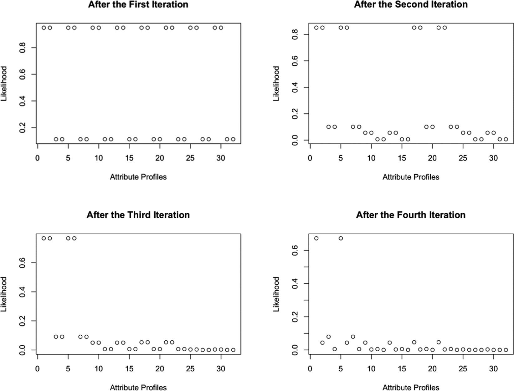


 Open access