


Nomenclature
- CDPR
-
cable-driven parallel robot
- MP
-
moving platform
- DoF
-
degree(s)-of-freedom
- VACTS
-
variable aerial cable towed system (see [Reference Li, Erskine, Caro and Chriette1])
- FD
-
forward dynamics
- ID
-
inverse dynamics
- EoM
-
equation of motion
- SDE
-
spring and damper element
- RSSLM
-
recursive sub-system-level Lagrange multiplier approach (see [Reference Mamidi and Bandyopadhyay2])
- MRFE
-
modified rigid finite element (see, e.g., [Reference Adamiec-Wójcik, Brzozowska, Drag and Wojciech3])
- GIM
-
generalised inertia matrix (see, e.g., [Reference Saha4])
- DAE
-
differential-algebraic equation
-
 $n_{\textrm{k}}$
-
$n_{\textrm{r}}$
CDPR
$n_{\textrm{k}}$
-
$n_{\textrm{r}}$
CDPR -
a CDPR with distinct
$n_{\textrm{k}}$
exit and
$n_{\textrm{r}}$
anchoring points of cables (see, e.g., [Reference Pott5], pp.
$29$
-
$30$
) -
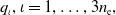
$\boldsymbol{{q}},{\dot{\boldsymbol{{q}}}},{\ddot{\boldsymbol{{q}}}} \in{\mathbb{R}^{n}}$
-
joint positions, velocities and accelerations, respectively
-
${\boldsymbol{{M}}} \in GL_{n}({\mathbb{R}})$
-
GIM of the robot
-
${\boldsymbol{{C}}} \in{\mathbb{R}^{n \times n}}$
-
centripetal and Coriolis matrix (see Eq. (2))
-
$\boldsymbol{{G}} \in{\mathbb{R}^{n}}$
-
generalised forces due to the gravitational potential
-
${\boldsymbol{\tau }^{\textrm{s}}} \in{\mathbb{R}^{n}}$
-
generalised forces due to the SDEs
-
${\boldsymbol{\tau }^{\textrm{c}}} \in{\mathbb{R}^{n}}$
-
generalised constraint forces (see Eq. (6))
-
$\boldsymbol{\eta } \in{\mathbb{R}^{m}}$
-
constraint functions
-
$\boldsymbol{\lambda } \in{\mathbb{R}^{m}}$
-
Lagrange multipliers appearing in the EoM (see Eq. (1))


1. Introduction
A cable-driven parallel robot (CDPR) manipulates the motion of a moving platform (MP) with the help of multiple cables connected to it. The CDPRs provide large workspaces, low inertias and high load-carrying capacities compared to their self-weights. Nevertheless, the analyses of these robots’ mechanics are challenging due to the cables’ unilaterality, that is, the ability to pull but not push, anisotropic material properties causing deflections to occur in different time scales, sagging due to their own weights and non-rigidity leading to large degrees-of-freedom (DoF). The actuation schemes employed in CDPRs also differ significantly from conventional manipulators with rigid links. Following the classification proposed in ref. [Reference Merlet6], the two kinds of actuation schemes commonly used in CDPRs are designated in this article as Type I and Type II, respectively. In the case of Type I CDPRs, the MP is manipulated by changing the lengths of the cables hoisting it. The cables themselves are fed and retrieved via stationary guidance systems (see, e.g., Fig. 2.1 in ref. [Reference Pott5], p.
 $17$
). In contrast, in Type II CDPRs, the cables’ lengths are held constant, whereas their terminal points (i.e., the ones not connected to the MP) are moved. These terminal points are known in CDPR parlance as the exit points of the cables (see Fig. 2).
$17$
). In contrast, in Type II CDPRs, the cables’ lengths are held constant, whereas their terminal points (i.e., the ones not connected to the MP) are moved. These terminal points are known in CDPR parlance as the exit points of the cables (see Fig. 2).
The primary focus of the present work is to develop a modular computational framework to simulate the dynamics of Type II CDPRs with cable models closer to the physical system, given the kinematic or dynamic actuation inputs. Also, extend the analyses to those scenarios where Type I actuation is applied simultaneously by employing the existing recursive forward dynamics algorithms for computational efficiency. The motivation for the above-mentioned directions of research is presented below vis-à-vis the previous works in this field.
The modularity of the proposed framework helps accommodate diverse architectures and actuators employed for different applications of Type II CDPRs in the past. For instance, the Wirepuller-Arm-driven Redundant Parallel manipulator, an
 $8$
-
$8$
-
 $3$
CDPR proposed in ref. [Reference Maeda, Tadokoro, Takamori, Hiller and Verhoeven7] for quick assembly of light payloads, employs arms driven by motors to manipulate the exit points of the cables. In ref. [Reference Cheng, Fink, Kumar and Pang8], mobile robots were employed for cooperative towing of the MPs of planar
$3$
CDPR proposed in ref. [Reference Maeda, Tadokoro, Takamori, Hiller and Verhoeven7] for quick assembly of light payloads, employs arms driven by motors to manipulate the exit points of the cables. In ref. [Reference Cheng, Fink, Kumar and Pang8], mobile robots were employed for cooperative towing of the MPs of planar
 $2$
-
$2$
-
 $2$
and
$2$
and
 $3$
-
$3$
-
 $3$
CDPRs with applications in warehouse operations. Likewise, a spatial
$3$
CDPRs with applications in warehouse operations. Likewise, a spatial
 $3$
-
$3$
-
 $3$
CDPR actuated by aerial vehicles with potential applications in rescue operations and heavy payload transfers was demonstrated in ref. [Reference Michael, Fink and Kumar9].
$3$
CDPR actuated by aerial vehicles with potential applications in rescue operations and heavy payload transfers was demonstrated in ref. [Reference Michael, Fink and Kumar9].
Further, the inclusion of simultaneous utilisation of both kinds of actuation schemes in the scope of the developed framework accommodates the following application scenarios. The Type II actuation was used for the active reconfiguration
Footnote
1
of a Type I CDPR in the Large Vessel Interface Lift-on and Lift-off (LVI Lo/Lo) crane system. It was designed to minimise the relative motions between the containers and ships while transferring cargo between two ships in the open seas with the help of a Type I actuated
 $8$
-
$8$
-
 $8$
CDPR attached to the end-effector of a serial crane (see, e.g., ref. [Reference Kery, Hughes, May, Kjolseth, Pang, Thomas, Treakle and Liut10]). A similar idea for micro-macro manipulation in ship replenishment was presented in ref. [Reference Oh, Ryu and Agrawal11], where the winches of a Type I suspended
$8$
CDPR attached to the end-effector of a serial crane (see, e.g., ref. [Reference Kery, Hughes, May, Kjolseth, Pang, Thomas, Treakle and Liut10]). A similar idea for micro-macro manipulation in ship replenishment was presented in ref. [Reference Oh, Ryu and Agrawal11], where the winches of a Type I suspended
 $6$
-
$6$
-
 $6$
CDPR were attached to a helicopter. Further, in ref. [Reference Zheng, Lin, Wu and Mitrouchev12], a Type I suspended
$6$
CDPR were attached to a helicopter. Further, in ref. [Reference Zheng, Lin, Wu and Mitrouchev12], a Type I suspended
 $3$
-
$3$
-
 $3$
CDPR was proposed to displace its winches via trolleys over rails and attain control of the 6 DoF of the MP for cargo handling. A Variable Aerial Cable Towed System (VACTS) was introduced in ref. [Reference Li, Erskine, Caro and Chriette1] by fastening the winches of a Type I suspended
$3$
CDPR was proposed to displace its winches via trolleys over rails and attain control of the 6 DoF of the MP for cargo handling. A Variable Aerial Cable Towed System (VACTS) was introduced in ref. [Reference Li, Erskine, Caro and Chriette1] by fastening the winches of a Type I suspended
 $6$
-
$6$
-
 $6$
CDPR on four aerial vehicles to transfer loads in cluttered environments. Recently, the utility of FASTKIT, a Type I
$6$
CDPR on four aerial vehicles to transfer loads in cluttered environments. Recently, the utility of FASTKIT, a Type I
 $8$
-
$8$
-
 $8$
CDPR mounted on top of two mobile robots, was demonstrated in ref. [Reference Pedemonte, Rasheed, Marquez-Gamez, Long, Hocquard, Babin, Fouché, Caverot, Girin and Caro13] as a low-cost solution for logistics in small warehouses.
$8$
CDPR mounted on top of two mobile robots, was demonstrated in ref. [Reference Pedemonte, Rasheed, Marquez-Gamez, Long, Hocquard, Babin, Fouché, Caverot, Girin and Caro13] as a low-cost solution for logistics in small warehouses.
The existing methodologies to solve the forward kinetostatic Footnote 2 problems of Type I CDPRs can be readily applied to those of the Type II CDPRs and vice versa due to the similarities in the inputs to these problems. In contrast, a clear distinction exists between the input actuator variables and the architecture parameters of these manipulators while analysing their dynamics due to the variations of the former with time. Hence, the formulations for forward dynamics (FD) analysis of Type II CDPRs are different from those of Type I robots (see, e.g., [Reference Masone, Bulthoff and Stegagno14]), requiring individual developments to incorporate the distinctions in cables’ actuation. Nevertheless, a few common features, such as the dynamic models of cables, moving platforms, and their interactions can be utilised from the formulations developed for Type I CDPRs. The current work employs one such modular and computationally efficient formulation recently reported in ref. [Reference Mamidi and Bandyopadhyay15] and focuses on the required additional developments.
The formulations of dynamics of Type II CDPRs wherein manned or unmanned aerial vehicles imparting motions of the cables’ exit points were extensively studied in the literature. The primary focus had been on the dynamic models of vehicles, their formations and interactions with the MP for applications in control. Consequently, the cable models were simplified significantly, that is, the cables were usually treated as massless and inelastic force transmission elements. The constrained equations of motion (EoM) were derived using either the Newton-Euler formulation, as in ref. [Reference Sreenath and Kumar16] or the Lagrangian formulation, as in ref. [Reference Lee, Sreenath and Kumar17], in a coordinate-free form. Such representations are compact and avoid the effects of singularities arising from the choice of parameters used to denote the rigid bodies’ orientations. Although these features are preferred to establish theoretical foundations, they are not ideal for performing FD simulations. Hence, it is typical to resort to commercially available software, for example, SimMechanics (Simscape Multibody) in ref. [Reference Masone, Bulthoff and Stegagno14], for FD simulations, even though inverse dynamics (ID) and control are based on custom-built dynamic models. Further, the benchmark dynamic models used for this purpose should be more accurate than those used to develop the controller. Therefore, monitoring such custom developments in the past is imperative to ensure that the framework developed in this work meets the necessary requirements.
For instance, in ref. [Reference Beloti-Pizetta, Santos-Brandao and Sarcinelli-Filho18], the elastic and damping properties of the cables of a planar
 $2$
-
$2$
-
 $1$
CDPR were introduced as massless spring and damper elements (SDEs) to demonstrate the effect of cables’ stretching on aerial vehicles connected to them. A custom framework called AuRoRA platform with virtual vehicle models was employed to perform the simulations. The cable tensions were first explicitly obtained from a separate dynamic model and were then provided as disturbances acting on the vehicles. Such a sequential treatment disregards the coupled dynamics, limiting their framework’s utility and fidelity of the results it produced. Contrary to the above-mentioned approach, in ref. [Reference Ariyibi and Tekinalp19], a commercial software, MSC ADAMS, was employed to model the cables as flexible aluminium bars, that is, massive and elastic, and then imported it to MATLAB/Simulink for realising the non-linear coupled dynamics of a
$1$
CDPR were introduced as massless spring and damper elements (SDEs) to demonstrate the effect of cables’ stretching on aerial vehicles connected to them. A custom framework called AuRoRA platform with virtual vehicle models was employed to perform the simulations. The cable tensions were first explicitly obtained from a separate dynamic model and were then provided as disturbances acting on the vehicles. Such a sequential treatment disregards the coupled dynamics, limiting their framework’s utility and fidelity of the results it produced. Contrary to the above-mentioned approach, in ref. [Reference Ariyibi and Tekinalp19], a commercial software, MSC ADAMS, was employed to model the cables as flexible aluminium bars, that is, massive and elastic, and then imported it to MATLAB/Simulink for realising the non-linear coupled dynamics of a
 $2$
-
$2$
-
 $2$
CDPR driven by quadrotors. Nevertheless, in specific situations where the MP is subjected to external disturbances or the vehicles are undergoing agile manoeuvres, the assumption that cables remain taut at all times is invalid (see, e.g., Section 4). Therefore, efforts towards incorporating the lateral and transverse flexibilities of cables into the dynamic model can also be seen in the following works.
$2$
CDPR driven by quadrotors. Nevertheless, in specific situations where the MP is subjected to external disturbances or the vehicles are undergoing agile manoeuvres, the assumption that cables remain taut at all times is invalid (see, e.g., Section 4). Therefore, efforts towards incorporating the lateral and transverse flexibilities of cables into the dynamic model can also be seen in the following works.
An early development in this regard is presented by Goodarzi et al. in ref. [Reference Goodarzi and Lee20], wherein the cables were modelled as serial chains of rigid links connected by universal joints, and quadcopters were used for moving their exit points. However, the EoM of the CDPR was developed using a coordinate-free form of the Lagrangian formulation with the intention of its utilisation in developing the controller. Recently, in ref. [Reference Rossomando, Rosales, Gimenez, Salinas, Soria, Sarcinelli-Filho and Carelli21], the cables were approximated as multiple lumped masses connected by SDEs to simulate the dynamics of a spatial
 $2$
-
$2$
-
 $1$
CDPR driven by quadcopters. Additionally, the effects of air resistance and contact forces from the ground were included in the model. The developed dynamic model was used to test the efficacy of the proposed controller.
$1$
CDPR driven by quadcopters. Additionally, the effects of air resistance and contact forces from the ground were included in the model. The developed dynamic model was used to test the efficacy of the proposed controller.
As is evident from the above survey of the existing literature, the dynamic models of cables considered in previous works have evolved from a massless inelastic one to a serial chain of point masses connected by SDEs. Therefore, the current work employs one such detailed cable model in developing the computational framework to meet the upcoming demands in this field. Furthermore, it addresses the shortcomings mentioned in the existing formulations of dynamics so that the proposed framework can perform the FD simulations in an efficient manner.
A few prominent works on the CDPRs that incorporate both Type II and Type I actuation schemes are mentioned below to re-emphasise that the research gaps addressed in this work are equally relevant in such scenarios. In ref. [Reference Oh, Ryu and Agrawal11], the Newton-Euler formulation was used to derive the EOM of a
 $6$
-
$6$
-
 $6$
CDPR with its winches mounted on a helicopter, assuming cables to be massless and inelastic force transmission elements. The FD simulations of the CDPR and helicopter, along with the proposed controllers, were performed using a framework developed in MATLAB/Simulink. The same approach was followed in the case of an
$6$
CDPR with its winches mounted on a helicopter, assuming cables to be massless and inelastic force transmission elements. The FD simulations of the CDPR and helicopter, along with the proposed controllers, were performed using a framework developed in MATLAB/Simulink. The same approach was followed in the case of an
 $8$
-
$8$
-
 $8$
CDPR suspended through a heavy airship in ref. [Reference Abdallah, Azouz, Beji and Abichou22] emphasising the added complexity due to the extra cable winches. In ref. [Reference Li, Erskine, Caro and Chriette1], such systems were referred to as VACTS and an experimental demonstration of their feasibility via a spatial
$8$
CDPR suspended through a heavy airship in ref. [Reference Abdallah, Azouz, Beji and Abichou22] emphasising the added complexity due to the extra cable winches. In ref. [Reference Li, Erskine, Caro and Chriette1], such systems were referred to as VACTS and an experimental demonstration of their feasibility via a spatial
 $3$
-
$3$
-
 $1$
CDPR was reported for the first time. These developments justify the extension of the proposed framework’s scope for analysing such systems. Moreover, the dynamic models of cables and the associated formulation of dynamics considered in the past are still in their preliminary stages compared to the proposed work. This limitation is also pertinent to systems other than VACTS, that is, those actuated by means other than aerial vehicles.
$1$
CDPR was reported for the first time. These developments justify the extension of the proposed framework’s scope for analysing such systems. Moreover, the dynamic models of cables and the associated formulation of dynamics considered in the past are still in their preliminary stages compared to the proposed work. This limitation is also pertinent to systems other than VACTS, that is, those actuated by means other than aerial vehicles.
For instance, in refs. [Reference Yamamoto, Yanai and Mohri23] and [Reference Zheng, Lin, Wu and Mitrouchev12], the cables were assumed to be massless and inelastic in deriving the EoM of a spatial
 $3$
-
$3$
-
 $3$
CDPR whose winches were moved using trolleys on rails. The incremental change over a decade is in considering the trolley’s dynamics in [Reference Zheng, Lin, Wu and Mitrouchev12], while it was ignored in [Reference Yamamoto, Yanai and Mohri23]. In the same category, an
$3$
CDPR whose winches were moved using trolleys on rails. The incremental change over a decade is in considering the trolley’s dynamics in [Reference Zheng, Lin, Wu and Mitrouchev12], while it was ignored in [Reference Yamamoto, Yanai and Mohri23]. In the same category, an
 $8$
-
$8$
-
 $8$
CDPR with four of its eight pulleys moved over vertical rails with applications in automated masonry was recently presented in ref. [Reference Bruckmann and Boumann24]. The cables were modelled as massless springs, and the EOM were obtained using the Newton-Euler formulation. Despite the existing limitations, a trend towards detailed cable models can be observed. A similar tendency exists in the cases where mobile vehicles on the ground were used to move the exit points of CDPRs.
$8$
CDPR with four of its eight pulleys moved over vertical rails with applications in automated masonry was recently presented in ref. [Reference Bruckmann and Boumann24]. The cables were modelled as massless springs, and the EOM were obtained using the Newton-Euler formulation. Despite the existing limitations, a trend towards detailed cable models can be observed. A similar tendency exists in the cases where mobile vehicles on the ground were used to move the exit points of CDPRs.
In ref. [Reference Zi, Qian, Ding and Kecskeméthy25], the cables were treated as massless and inelastic force transmission elements, and the EoM of a
 $3$
-
$3$
-
 $3$
CDPR with each cable connected to a mobile crane was established. Recently, in ref. [Reference Rasheed, Long, Roos and Caro26], the dynamic model of a spatial
$3$
CDPR with each cable connected to a mobile crane was established. Recently, in ref. [Reference Rasheed, Long, Roos and Caro26], the dynamic model of a spatial
 $4$
-
$4$
-
 $1$
CDPR attached to four Turtlebots, termed MoPICK, was developed in the V-REP environment. The cables were approximated to be serial chains of multiple massive cylindrical links connected by prismatic joints. In ref. [Reference Goodarzi, Korayem, Tourajizadeh and Nourizadeh27], the Rayleigh–Ritz method was employed to model the non-linear longitudinal vibrations of the cables of a mobile ICaSbot, that is, a
$1$
CDPR attached to four Turtlebots, termed MoPICK, was developed in the V-REP environment. The cables were approximated to be serial chains of multiple massive cylindrical links connected by prismatic joints. In ref. [Reference Goodarzi, Korayem, Tourajizadeh and Nourizadeh27], the Rayleigh–Ritz method was employed to model the non-linear longitudinal vibrations of the cables of a mobile ICaSbot, that is, a
 $6$
-
$6$
-
 $6$
CDPR mounted on a mobile base platform.
$6$
CDPR mounted on a mobile base platform.
The significant contributions of this work can be summarised as follows. As is apparent from the reported survey of the state-of-the-art, many combinations of actuators and CDPRs were investigated in the past. However, apart from a few recent attempts, little to no effort has been spent in bringing the forward dynamic models of Type II CDPRs closer to their physical realities. The present work bridges this gap by proposing a computational framework to comprehensively model and analyse the dynamics of Type II CDPRs with kinematic and dynamic actuation inputs.
The said framework is detailed and realistic; for example, it takes into consideration the inertia, elasticity and damping of the cables while modelling their dynamics. Also, it is modular by design. In this context, “modular” implies that the components of the CDPR, such as the cables, the MP and the driving mechanisms, are treated as independent sub-systems. It does not refer to different models of links and joints used to represent these sub-systems, as in ref. [Reference Cao, Dolovich, Schwab, Herder and Zhang28]. For instance, as shown in Figs. 3 and 5, the spatial
 $4$
-
$4$
-
 $4$
CDPR was notionally decomposed to four cables, an MP, and four quadcopters to perform the analysis. As such, the dynamic model of each can be developed in isolation, and then those can be integrated to define the dynamics of the CDPR as a whole. Naturally, different combinations can be created out of the same set of modules to generate multiple CDPRs.
$4$
CDPR was notionally decomposed to four cables, an MP, and four quadcopters to perform the analysis. As such, the dynamic model of each can be developed in isolation, and then those can be integrated to define the dynamics of the CDPR as a whole. Naturally, different combinations can be created out of the same set of modules to generate multiple CDPRs.
Further, the inputs to the analyses can be either the variations of forces imparted by the actuators or the changes in the locations of the cables’ exit points with time. The latter class of problems is addressed for the first time in the present work to the best of the knowledge of the authors.
A recursive sub-system-level Lagrange multiplier (RSSLM) FD algorithm, originally introduced in ref. [Reference Mamidi and Bandyopadhyay2], is employed to efficiently perform the computations in linear time. This work extends its applicability to include closed-loop rigid-flexible multi-body systems with rheonomic constraints for the first time. In addition, the generic nature of this framework for analysing CDPRs involving simultaneous application of both kinds of actuation is also demonstrated for the first time.
A brief overview of the existing dynamic models of CDPRs is presented in Section 2. The modifications necessary to incorporate the Type II actuation are elucidated in Section 3. The effectiveness of the proposed framework is demonstrated with the help of a spatial
 $4$
-
$4$
-
 $4$
CDPR in Section 4. In particular, its capability to incorporate different types of actuation is illustrated with the same example in Section 4.4. Finally, the discussions and conclusions of the present work are presented in Sections 5 and 6, respectively.
$4$
CDPR in Section 4. In particular, its capability to incorporate different types of actuation is illustrated with the same example in Section 4.4. Finally, the discussions and conclusions of the present work are presented in Sections 5 and 6, respectively.
2. Existing dynamic models of cable-Driven parallel robot
The dynamic model of CDPRs employed in the present work is an extension of those developed in refs. [Reference Mamidi and Bandyopadhyay2, Reference Mamidi and Bandyopadhyay15]. Therefore, a brief overview of these models is presented first for the sake of completeness.
The cables are modelled as serial chains of modified rigid finite elements (MRFEs), mentioned in refs.[Reference Adamiec-Wójcik, Brzozowska, Drag and Wojciech3]. As depicted in Fig. 1, each MRFE consists of two rigid links connected by a prismatic (P) joint, and these elements are connected to one another by a universal (U) joint. The axial deflections, considering both the axial stiffness and damping of the cables, are lumped together in the form of SDEs at the P joints. Similarly, those due to the transverse and lateral stiffness and damping properties are lumped together as the SDEs at the U joints.
A typical architecture of a modified rigid finite element, adopted from [Reference Adamiec-Wójcik, Drag and Wojciech29].

The MP was modelled as a rigid body connected in parallel to multiple serial chains of MRFEs. Effectively, the dynamic model of a CDPR without the inclusion of the effects of actuation was rendered equivalent to a rigid-flexible multi-body mechanical system with closed loops. The EoM of such systems are represented as follows:
 \begin{align}{\boldsymbol{{M}}}_j{\ddot{\boldsymbol{{q}}}} = \boldsymbol{{f}}_j + \sum _{i=1}^{u}\boldsymbol{{J}}_{{\boldsymbol{\eta }\boldsymbol{{q}}}_{i, j}}^\top \boldsymbol{\lambda }_i,\; j=1,\dots,v, \end{align}
where
 $v$
denotes the number of sub-systems, that is, cables and MP, and
$v$
denotes the number of sub-systems, that is, cables and MP, and
 $u$
represents the number of independent closed loops. The matrix
$u$
represents the number of independent closed loops. The matrix
 ${\boldsymbol{{M}}}_j \in GL_{n_j}({\mathbb{R}})$
is the
${\boldsymbol{{M}}}_j \in GL_{n_j}({\mathbb{R}})$
is the
 $j$
th sub-system’s generalised inertia matrix (GIM) (see, e.g., [Reference Saha4]), with
$j$
th sub-system’s generalised inertia matrix (GIM) (see, e.g., [Reference Saha4]), with
 $n_j$
being the number of joints in that sub-system. The vector
$n_j$
being the number of joints in that sub-system. The vector
 $\boldsymbol{{q}}_j \in{\mathbb{R}^{n_j}}$
represents the joint displacements,
$\boldsymbol{{q}}_j \in{\mathbb{R}^{n_j}}$
represents the joint displacements,
 ${\dot{\boldsymbol{{q}}}}_j \in{\mathbb{R}^{n_j}}$
their velocities and
${\dot{\boldsymbol{{q}}}}_j \in{\mathbb{R}^{n_j}}$
their velocities and
 ${\ddot{\boldsymbol{{q}}}}_j \in{\mathbb{R}^{n_j}}$
their accelerations. The first term on the right side of the equation,
${\ddot{\boldsymbol{{q}}}}_j \in{\mathbb{R}^{n_j}}$
their accelerations. The first term on the right side of the equation,
 $\boldsymbol{{f}}_j \in{\mathbb{R}^{n_j}}$
, incorporates the contributions of the generalised forces imparted by the environment (
$\boldsymbol{{f}}_j \in{\mathbb{R}^{n_j}}$
, incorporates the contributions of the generalised forces imparted by the environment (
 $\boldsymbol{\tau }_j$
), due to the SDEs (
$\boldsymbol{\tau }_j$
), due to the SDEs (
 $\boldsymbol{\tau }_j^{\textrm{s}}$
), the centripetal and Coriolis accelerations
$\boldsymbol{\tau }_j^{\textrm{s}}$
), the centripetal and Coriolis accelerations
 $\left (\sum _{k=1}^u{\boldsymbol{{C}}}_{j,k}{\dot{\boldsymbol{{q}}}}_k\right )$
and the gravity load (
$\left (\sum _{k=1}^u{\boldsymbol{{C}}}_{j,k}{\dot{\boldsymbol{{q}}}}_k\right )$
and the gravity load (
 $\boldsymbol{{G}}_j$
). It is computed as the following sum:
$\boldsymbol{{G}}_j$
). It is computed as the following sum:
 \begin{align} \boldsymbol{{f}}_j = \boldsymbol{\tau }_j +{\boldsymbol{\tau }_j^{\textrm{s}}} - \sum _{k=1}^v{\boldsymbol{{C}}}_{j, k}{\dot{\boldsymbol{{q}}}}_k - \boldsymbol{{G}}_j. \end{align}
The second term in Eq. (1) indicates the generalised constraint forces necessary for maintaining the connectivity between different sub-systems. The reaction forces at such common points between a pair of sub-systems are denoted by
 $\boldsymbol{\lambda }_i \in{\mathbb{R}^{m_i}}$
, with
$\boldsymbol{\lambda }_i \in{\mathbb{R}^{m_i}}$
, with
 $m_i$
being the minimum number of constraints required to ensure the integrity of
$m_i$
being the minimum number of constraints required to ensure the integrity of
 $i$
th loop. The distribution of reaction forces at every joint was computed by transforming these via the sub-matrices of constraint Jacobian matrix,
$i$
th loop. The distribution of reaction forces at every joint was computed by transforming these via the sub-matrices of constraint Jacobian matrix,
 $\boldsymbol{{J}}_{{\boldsymbol{\eta }\boldsymbol{{q}}}_{i, j}} \in{\mathbb{R}^{m_i \times n_j}}$
. These transformations are computed from the following constraint functions that need to be satisfied at all times to ensure the intactness of
$\boldsymbol{{J}}_{{\boldsymbol{\eta }\boldsymbol{{q}}}_{i, j}} \in{\mathbb{R}^{m_i \times n_j}}$
. These transformations are computed from the following constraint functions that need to be satisfied at all times to ensure the intactness of
 $i$
th closed loop:
$i$
th closed loop:
 \begin{align}& \boldsymbol{\eta }_i (\boldsymbol{{q}}) = \textbf{0}, \end{align}
 \begin{align} \Rightarrow \; & \dot{\boldsymbol{\eta }}_i = \sum _{j=1}^{v}{\frac{\partial \boldsymbol{\eta }_i}{\partial \boldsymbol{{q}}_j }} \dot{\boldsymbol{{q}}}_j =\sum _{j=1}^{v} \boldsymbol{{J}}_{{\boldsymbol{\eta }\boldsymbol{{q}}}_{i, j}} \dot{\boldsymbol{{q}}}_j=\textbf{0}, \textrm{ where } \boldsymbol{{J}}_{{\boldsymbol{\eta }\boldsymbol{{q}}}_{i, j}} ={\frac{\partial \boldsymbol{\eta }_i}{\partial \boldsymbol{{q}}_j }}. \end{align}
The additional conditions required for the computation of the unknown reaction forces,
 $\boldsymbol{\lambda }_i$
, are obtained as:
$\boldsymbol{\lambda }_i$
, are obtained as:
 \begin{align} \ddot{\boldsymbol{\eta }}_i ={\frac{\textrm{d} \dot{\boldsymbol{\eta }}_i}{\textrm{d} t}} = \sum _{j=1}^{v} \left ( \boldsymbol{{J}}_{{\boldsymbol{\eta }\boldsymbol{{q}}}_{i, j}} \ddot{\boldsymbol{{q}}}_j + \dot{\boldsymbol{{J}}}_{{\boldsymbol{\eta }\boldsymbol{{q}}}_{i, j}} \dot{\boldsymbol{{q}}}_j \right ) = \textbf{0}. \end{align}
A computationally efficient RSSLM approach was employed to determine the reaction forces
 $\boldsymbol{\lambda }_i$
and the joint accelerations
$\boldsymbol{\lambda }_i$
and the joint accelerations
 ${\ddot{\boldsymbol{{q}}}}_j$
at desired instances of time using Eq. (1) and Eq. (5) for specified joint positions
${\ddot{\boldsymbol{{q}}}}_j$
at desired instances of time using Eq. (1) and Eq. (5) for specified joint positions
 $\boldsymbol{{q}}_j$
and velocities
$\boldsymbol{{q}}_j$
and velocities
 ${\dot{\boldsymbol{{q}}}}_j$
.
${\dot{\boldsymbol{{q}}}}_j$
.
The incorporation of the Type I actuation through time-varying lengths of the rigid links of MRFEs, in ref. [Reference Mamidi and Bandyopadhyay15], induced an explicit dependence of every term in Eq. (1) on time, that is:
 \begin{align}{{\boldsymbol{{M}}}}_j (t){{\ddot{\boldsymbol{{q}}}}}_j + \sum _{k=1}^v{\boldsymbol{{C}}}_{j, k}(t){\dot{\boldsymbol{{q}}}}_k + \boldsymbol{{G}}_j (t) ={\boldsymbol{\tau }_j^{\textrm{s}}} (t) + \boldsymbol{\tau }_j +{\boldsymbol{\tau }_j^{\textrm{c}}}(t),\;j=1,\dots,v. \end{align}
Also, the matrix
 $\boldsymbol{{C}}$
represents generalised forces caused by the changing inertia of cables and those associated with centripetal and Coriolis accelerations. The linear time complexity of the RSSLM approach is retained even after such necessary modifications.
$\boldsymbol{{C}}$
represents generalised forces caused by the changing inertia of cables and those associated with centripetal and Coriolis accelerations. The linear time complexity of the RSSLM approach is retained even after such necessary modifications.
The modifications required to incorporate the Type II actuation in the same framework are presented in the next section.
3. Extension of the dynamic model to include Type II actuation
A typical scenario of the Type II actuation in CDPRs is illustrated in Fig. 2. Multiple driving mechanisms, denoted by
 $\textrm{D}_k$
, manipulate the positions of the exit points of cables,
$\textrm{D}_k$
, manipulate the positions of the exit points of cables,
 $\boldsymbol{{b}}_k$
. As mentioned in Section 1, these mechanisms could be aerial vehicles, mobile robots, or gantry cranes. Moreover, all the cables could be connected to the same rigid body, as in the case of a crane, or connected to multiple robots for cooperative transportation. This provision is made feasible due to the modular nature of the proposed framework, which can accommodate any other variation in the components of the system as well.
$\boldsymbol{{b}}_k$
. As mentioned in Section 1, these mechanisms could be aerial vehicles, mobile robots, or gantry cranes. Moreover, all the cables could be connected to the same rigid body, as in the case of a crane, or connected to multiple robots for cooperative transportation. This provision is made feasible due to the modular nature of the proposed framework, which can accommodate any other variation in the components of the system as well.
A schematic representation of a typical type II CDPR. The
 $k$
th cable, labelled as
$k$
th cable, labelled as
 $C_k$
, is attached to the moving platform at
$C_k$
, is attached to the moving platform at
 $\xi _r$
and connected to the driving mechanism
$\xi _r$
and connected to the driving mechanism
 $\textrm{D}_k$
at
$\textrm{D}_k$
at
 $\boldsymbol{{b}}_k$
. The point
$\boldsymbol{{b}}_k$
. The point
 $\boldsymbol{{b}}_k$
is known as the exit point (described in section 1).
$\boldsymbol{{b}}_k$
is known as the exit point (described in section 1).

The locations of the exit points of the cables are treated as immobile in refs. [Reference Mamidi and Bandyopadhyay2, Reference Mamidi and Bandyopadhyay15]. However, to analyse the dynamics of Type II CDPRs, the motions of these points must be considered. First, the necessary modifications to the computational model presented in ref. [Reference Mamidi and Bandyopadhyay2] are elucidated. Next, the formulations of dynamics are characterised depending on the kinds of inputs supplied to the analyses, that is,
-
1. Availability of the forces applied on the exit points or the actuator efforts of the driving mechanisms (attached to these points), and
-
2. Provision of the trajectories tracked by the exit points of cables.
Finally, the efficacy of the proposed formulations is demonstrated using the incompletely restrained spatial suspended
 $4$
-
$4$
-
 $4$
CDPR as an example.
$4$
CDPR as an example.
3.1. Forward dynamics formulation
The dynamic model of the cable is modified to accommodate the relative motions of their exit points with respect to the global frame of reference
 $\boldsymbol{{o}}$
-
$\boldsymbol{{o}}$
-
 $X_0Y_0Z_0$
. Due to these additional DoF, the configuration of cable
$X_0Y_0Z_0$
. Due to these additional DoF, the configuration of cable
 $C_k$
is updated to:
$C_k$
is updated to:
 \begin{align} \boldsymbol{{q}}_j = \left [\boldsymbol{{b}}_k^\top, q_1,\dots,q_{3{n_{\textrm{e}}}}\right ]^\top \in{\mathbb{R}^{3 ({n_{\textrm{e}}}+1)}},\; j=k=1,\dots,{n_{\textrm{k}}}. \end{align}
In Eq. (7), the symbol
 $\boldsymbol{{b}}_k$
denotes the position of the exit point of cable
$\boldsymbol{{b}}_k$
denotes the position of the exit point of cable
 $C_k$
, whereas
$C_k$
, whereas
 $q_\iota, \iota =1,\dots,3{n_{\textrm{e}}},$
with
$q_\iota, \iota =1,\dots,3{n_{\textrm{e}}},$
with
 $n_{\textrm{e}}$
being the number of elements, represent the configuration of the cable. The number of cables is denoted by
$n_{\textrm{e}}$
being the number of elements, represent the configuration of the cable. The number of cables is denoted by
 $n_{\textrm{k}}$
. Further changes to the formulation of dynamics based on the nature of inputs provided to the analyses are outlined below.
$n_{\textrm{k}}$
. Further changes to the formulation of dynamics based on the nature of inputs provided to the analyses are outlined below.
3.1.1. Inputs in the form of forces applied at the exit points of cables
The first kind of inputs considered in the following is the forces exerted by the driving mechanisms on the cables. In such cases, assuming no other external forces are acting on the cables, the vector of external generalised forces of cable
 $C_k$
has the following structure:
$C_k$
has the following structure:
 \begin{align} \boldsymbol{\tau }_k = \left [\boldsymbol{\lambda }_i^\top, 0, \dots, 0\right ]^\top \in{\mathbb{R}^{3 ({n_{\textrm{e}}}+1)}},\; k=1,\dots,{n_{\textrm{k}}},\; i={n_{\textrm{k}}}+ k. \end{align}
The force
 $\boldsymbol{\lambda }_{{n_{\textrm{k}}}+ k}$
in Eq. (8) acts at the exit point of cable
$\boldsymbol{\lambda }_{{n_{\textrm{k}}}+ k}$
in Eq. (8) acts at the exit point of cable
 $C_k$
.
$C_k$
.
Alternatively, the generalised forces internal to the actuators of the driving mechanisms, denoted by
 $\boldsymbol{\tau }_i$
, could be specified as inputs to the analyses when there is no provision for direct measurement of
$\boldsymbol{\tau }_i$
, could be specified as inputs to the analyses when there is no provision for direct measurement of
 $\boldsymbol{\lambda }_i$
. In such scenarios, as depicted in Fig. 3, every mechanism
$\boldsymbol{\lambda }_i$
. In such scenarios, as depicted in Fig. 3, every mechanism
 $\textrm{D}_k,\,k=1,\dots,{n_{\textrm{k}}}$
, is treated as a separate sub-system of the CDPR to compute the required restraining forces at the corresponding exit point.
$\textrm{D}_k,\,k=1,\dots,{n_{\textrm{k}}}$
, is treated as a separate sub-system of the CDPR to compute the required restraining forces at the corresponding exit point.
Driving mechanisms,
 $\textrm{D}_k,\,k=1,\dots,{n_{\textrm{k}}}$
, as separate sub-systems of a Type II CDPR. The symbol
$\textrm{D}_k,\,k=1,\dots,{n_{\textrm{k}}}$
, as separate sub-systems of a Type II CDPR. The symbol
 $\boldsymbol{\tau }_i, i={n_{\textrm{k}}}+k,$
denotes the internal actuator forces of the
$\boldsymbol{\tau }_i, i={n_{\textrm{k}}}+k,$
denotes the internal actuator forces of the
 $k$
th driving mechanism and
$k$
th driving mechanism and
 $\boldsymbol{\lambda }_i$
represents the reaction forces at the exit point
$\boldsymbol{\lambda }_i$
represents the reaction forces at the exit point
 $\boldsymbol{{b}}_k$
of the cable
$\boldsymbol{{b}}_k$
of the cable
 $C_k$
.
$C_k$
.

At first, the connectivity between the sub-systems
 $\textrm{D}_k$
and
$\textrm{D}_k$
and
 $C_k$
is ensured by introducing the action-reaction pair of forces, denoted by
$C_k$
is ensured by introducing the action-reaction pair of forces, denoted by
 $\boldsymbol{\lambda }_i$
. Subsequently,
$\boldsymbol{\lambda }_i$
. Subsequently,
 $\boldsymbol{\lambda }_i$
are computed from the imposition of additional constraint equations,
$\boldsymbol{\lambda }_i$
are computed from the imposition of additional constraint equations,
 $\boldsymbol{\eta }_i=\textbf{0}$
, where:
$\boldsymbol{\eta }_i=\textbf{0}$
, where:
 \begin{align} \boldsymbol{\eta }_i = \boldsymbol{{b}}_k -{\boldsymbol{{e}}}_k,\; k=1,\dots,{n_{\textrm{k}}},\,i={n_{\textrm{k}}}+k. \end{align}
In Eq. (9), the location of the leading end of cable
 $C_k$
is denoted by
$C_k$
is denoted by
 $\boldsymbol{{b}}_k$
and its attachment point on
$\boldsymbol{{b}}_k$
and its attachment point on
 $\textrm{D}_k$
by
$\textrm{D}_k$
by
 ${\boldsymbol{{e}}}_k$
.
${\boldsymbol{{e}}}_k$
.
In summary, the above formulation can handle inputs either in the form of forces directly applied on the exit points of cables or those that are internal to the actuators of the driving mechanisms. However, there can be many situations where the inputs are available in the form of motions of the exit points rather than the forces acting on them. One instance of such a scenario can be where the exit points of the cables are being carried by individual aerial vehicles, such as quadrotors or helicopters – instead of incorporating their dynamics into the overall model, one can simply track their motions and use those as kinematic inputs to the overall system. Analyses of such systems are discussed next.
3.1.2. Inputs in the form of trajectories tracked by the exit points of cables
The second kind of inputs to the analyses are the trajectories of the exit points of cables. As shown in Fig. 4, the point
 $\boldsymbol{{b}}_k$
of cable
$\boldsymbol{{b}}_k$
of cable
 $C_k$
is considered to follow the input trajectory
$C_k$
is considered to follow the input trajectory
 ${\boldsymbol{{e}}}_k(t)$
. Consequently, the inputs at some of the joints will be kinematic while the rest are dynamic in nature. Therefore, simulation of the CDPR requires a hybrid approach, that is, both the FD and ID analyses as classified in [Reference Featherstone30], pp.
${\boldsymbol{{e}}}_k(t)$
. Consequently, the inputs at some of the joints will be kinematic while the rest are dynamic in nature. Therefore, simulation of the CDPR requires a hybrid approach, that is, both the FD and ID analyses as classified in [Reference Featherstone30], pp.
 $171$
–
$171$
–
 $172$
. Such problems of CDPRs are addressed for the first time in the present work, to the best of the authors’ knowledge.
$172$
. Such problems of CDPRs are addressed for the first time in the present work, to the best of the authors’ knowledge.
Representative trajectories
 $e_k(t)$
of the exit points
$e_k(t)$
of the exit points
 $\boldsymbol{{b}}_k$
of cables
$\boldsymbol{{b}}_k$
of cables
 $C_k$
in Type II CDPRs. The reaction forces acting at the exit point
$C_k$
in Type II CDPRs. The reaction forces acting at the exit point
 $\boldsymbol{{b}}_k$
are denoted by
$\boldsymbol{{b}}_k$
are denoted by
 $\boldsymbol{\lambda }_{{n_{\textrm{k}}}+k}$
.
$\boldsymbol{\lambda }_{{n_{\textrm{k}}}+k}$
.

In the present work, the hybrid dynamic analysis of the robot is circumvented by introducing the following constraint equations:
 \begin{align} \boldsymbol{\eta }_i(\boldsymbol{{b}}_k, t) \,:\!=\, \boldsymbol{{b}}_k -{\boldsymbol{{e}}}_k(t) = 0,\; k=1,\dots,{n_{\textrm{k}}},\, i={n_{\textrm{k}}}+k. \end{align}
Clearly, Eq. (10) represents rheonomic constraints,Footnote
3
that is, they depend explicitly on time. Therefore, the associated Lagrange multipliers, denoted by
 $\boldsymbol{\lambda }_i$
, are also functions of time. Specifically, differentiating
$\boldsymbol{\lambda }_i$
, are also functions of time. Specifically, differentiating
 $\boldsymbol{\eta }_i$
twice results in the following expression:
$\boldsymbol{\eta }_i$
twice results in the following expression:
 \begin{align}{\frac{\textrm{d} \boldsymbol{\eta }_i}{\textrm{d} t}} &={\frac{\textrm{d} }{\textrm{d} t}} \left ({\frac{\partial \boldsymbol{\eta }_i}{\partial t }} + \sum _{j=1}^v \boldsymbol{{J}}_{\boldsymbol{\eta }\boldsymbol{{q}}_{i,j}}{\dot{\boldsymbol{{q}}}}_j\right ) \nonumber \\ &={\frac{\partial ^2 \boldsymbol{\eta }_i}{\partial t^2}} + \sum _{j=1}^v \left ({\frac{\partial }{\partial q_j }} \left ({\frac{\partial \boldsymbol{\eta }_i}{\partial t }}\right ){\dot{\boldsymbol{{q}}}}_j + \boldsymbol{{J}}_{\boldsymbol{\eta }\boldsymbol{{q}}_{i,j}}{\ddot{\boldsymbol{{q}}}}_j +{\frac{\textrm{d} }{\textrm{d} t}}\left (\boldsymbol{{J}}_{\boldsymbol{\eta }\boldsymbol{{q}}_{i,j}}\right ){\dot{\boldsymbol{{q}}}}_j \right ) . \end{align}
Equation (11) may be simplified significantly by taking into cognisance the following.
-
1. The variations of
$\boldsymbol{\eta }_i$
w.r.t. time and the configuration variables,
$\boldsymbol{{q}}_j$
, are mutually independent, hence
${\frac{\partial }{\partial q_j }}\left ({\frac{\partial \boldsymbol{\eta }_i}{\partial t }}\right ) ={\textbf{0}}$
. -
2. The matrix
$\boldsymbol{{J}}_{\boldsymbol{\eta }\boldsymbol{{q}}_{i,j}}$
is of constant nature, since its entries are either ones or zeros. Therefore,
${\frac{\textrm{d} }{\textrm{d} t}}\left (\boldsymbol{{J}}_{\boldsymbol{\eta }\boldsymbol{{q}}_{i,j}}\right ) ={\textbf{0}}$
.


With these, Eq. (11) reduces to:
 \begin{align} &{\frac{\textrm{d}^2 \boldsymbol{\eta }_i}{\textrm{d} t^2}} ={\frac{\partial ^2 \boldsymbol{\eta }_i}{\partial t^2}} + \sum _{j=1}^v \boldsymbol{{J}}_{\boldsymbol{\eta }\boldsymbol{{q}}_{i,j}}{\ddot{\boldsymbol{{q}}}}_j ={\textbf{0}},\; i={n_{\textrm{k}}}+1,\dots,2{n_{\textrm{k}}}. \end{align}
The key difference between the above form of the loop-closure equation and that associated with the scleronomic types (as in Eq. (5)) is the additional term
 $\frac{\partial ^2 \boldsymbol{\eta }_i}{\partial t^2}$
, accounting for the explicit dependence of
$\frac{\partial ^2 \boldsymbol{\eta }_i}{\partial t^2}$
, accounting for the explicit dependence of
 $\boldsymbol{\eta }_i$
on time. Consequently, the expression of the residual constraint accelerations
$\boldsymbol{\eta }_i$
on time. Consequently, the expression of the residual constraint accelerations
 $\boldsymbol{\psi }_i$
(see Eq. (15)) is modified to:
$\boldsymbol{\psi }_i$
(see Eq. (15)) is modified to:
 \begin{align} \boldsymbol{\psi }_i ={\frac{\partial ^2 \boldsymbol{\eta }_i}{\partial t^2}} + \sum _{j=1}^v \boldsymbol{{J}}_{\boldsymbol{\eta }\boldsymbol{{q}}_{i,j}} \boldsymbol{{a}}_j,\; i={n_{\textrm{k}}}+1,\dots,2{n_{\textrm{k}}}. \end{align}
In Eq. (13), the symbol
 $\boldsymbol{{a}}_j \in{\mathbb{R}^{n_j}}$
denotes the unconstrained joint accelerations of the
$\boldsymbol{{a}}_j \in{\mathbb{R}^{n_j}}$
denotes the unconstrained joint accelerations of the
 $j$
th sub-system and it is given by:
$j$
th sub-system and it is given by:
 \begin{align} \boldsymbol{{a}}_j ={{\boldsymbol{{M}}}_j}^{-1} \boldsymbol{{f}}_j,\;j=1,\dots,v, \end{align}
where
 $\boldsymbol{{f}}_j$
is the cumulative effect of the generalised forces devoid of the inertial and constrained forces acting on the
$\boldsymbol{{f}}_j$
is the cumulative effect of the generalised forces devoid of the inertial and constrained forces acting on the
 $j$
th sub-system, as in Eq. (2). Finally, the Lagrange multipliers can be computed using the same expressions reported in ref. [Reference Mamidi and Bandyopadhyay2], that is:
$j$
th sub-system, as in Eq. (2). Finally, the Lagrange multipliers can be computed using the same expressions reported in ref. [Reference Mamidi and Bandyopadhyay2], that is:
 \begin{align} \sum _{s=1}^{u} \boldsymbol{{A}}_{i, s} \boldsymbol{\lambda }_s + \boldsymbol{\psi }_i = \textbf{0},\;i=1,\dots,u,\textrm{ and }u= 2{n_{\textrm{k}}}, \end{align}
where
 $\boldsymbol{{A}}_{i, s} \in{\mathbb{R}^{m_i \times m_i}}$
is the sub-matrix of the generalised inertia constraint matrix, mentioned in ref. [Reference Koul, Shah, Saha and Manivannan31]. Effectively, by virtue of the generalisations mentioned above, the modified RSSLM approach can simulate the dynamics of Type II CDPRs even when the trajectories of the driving mechanisms are provided as inputs.
$\boldsymbol{{A}}_{i, s} \in{\mathbb{R}^{m_i \times m_i}}$
is the sub-matrix of the generalised inertia constraint matrix, mentioned in ref. [Reference Koul, Shah, Saha and Manivannan31]. Effectively, by virtue of the generalisations mentioned above, the modified RSSLM approach can simulate the dynamics of Type II CDPRs even when the trajectories of the driving mechanisms are provided as inputs.
4. Illustrative examples
The utility of the modified computational model is demonstrated on an incompletely restrained suspended
 $4$
-
$4$
-
 $4$
CDPR. The details related to the architecture of the robot and the notations used in the formulation of dynamics are delineated in Section 4.1. Also, a rudimentary model used for detecting the contact between the MP and the ground so as to prevent the MP from penetrating the ground is described in Appendix B. In the first case study, the transfer of load from an initial pose to a final one based on the input trajectories of the exit points of cables is demonstrated. In the second one, four quadcopters are used to manipulate the motions of these exit points. The response of the CDPR when one of those quadcopters fails mid-flight is examined. In the final case study, the response of the robot is investigated when different types of actuation, namely, Types I & II, are simultaneously applied.
$4$
CDPR. The details related to the architecture of the robot and the notations used in the formulation of dynamics are delineated in Section 4.1. Also, a rudimentary model used for detecting the contact between the MP and the ground so as to prevent the MP from penetrating the ground is described in Appendix B. In the first case study, the transfer of load from an initial pose to a final one based on the input trajectories of the exit points of cables is demonstrated. In the second one, four quadcopters are used to manipulate the motions of these exit points. The response of the CDPR when one of those quadcopters fails mid-flight is examined. In the final case study, the response of the robot is investigated when different types of actuation, namely, Types I & II, are simultaneously applied.
4.1. Architecture of a 4-4 cable-driven parallel robot
A
 $4$
-
$4$
-
 $4$
CDPR consists of four cables
$4$
CDPR consists of four cables
 $C_1,\dots,C_4$
connected to the MP at
$C_1,\dots,C_4$
connected to the MP at
 $\boldsymbol{\xi }_1,\dots,\boldsymbol{\xi }_4,$
and to the driving mechanisms at
$\boldsymbol{\xi }_1,\dots,\boldsymbol{\xi }_4,$
and to the driving mechanisms at
 $\boldsymbol{{b}}_1,\dots,\boldsymbol{{b}}_4$
. It is decomposed into four cables and an MP, as shown in Fig. 5. The length, width and height of the MP are represented by
$\boldsymbol{{b}}_1,\dots,\boldsymbol{{b}}_4$
. It is decomposed into four cables and an MP, as shown in Fig. 5. The length, width and height of the MP are represented by
 ${l_{\textrm{m}}},{w_{\textrm{m}}},{h_{\textrm{m}}},$
respectively. Since the local frame of reference
${l_{\textrm{m}}},{w_{\textrm{m}}},{h_{\textrm{m}}},$
respectively. Since the local frame of reference
 $\boldsymbol{\xi }_{\textrm{c}}$
-
$\boldsymbol{\xi }_{\textrm{c}}$
-
 $X_aY_aZ_a$
is considered identical to the fixed one
$X_aY_aZ_a$
is considered identical to the fixed one
 $\boldsymbol{{o}}$
-
$\boldsymbol{{o}}$
-
 $X_0Y_0Z_0$
at the initial configuration, the ZYZ convention of Euler angles used for representing its orientation in the previous works, for example, [Reference Mamidi and Bandyopadhyay2], will lead to a parametric singularity (see, e.g., [Reference Shah, Saha and Dutt32], pp.
$X_0Y_0Z_0$
at the initial configuration, the ZYZ convention of Euler angles used for representing its orientation in the previous works, for example, [Reference Mamidi and Bandyopadhyay2], will lead to a parametric singularity (see, e.g., [Reference Shah, Saha and Dutt32], pp.
 $51$
–
$51$
–
 $52$
). Therefore, the XYZ convention is used in this case to circumvent the singularity, and the corresponding DH parameters are listed in Table I.
$52$
). Therefore, the XYZ convention is used in this case to circumvent the singularity, and the corresponding DH parameters are listed in Table I.
Notional decomposition of the
 $4$
-
$4$
-
 $4$
cable-driven parallel robot into four cables and a moving platform.
$4$
cable-driven parallel robot into four cables and a moving platform.

The action-reaction forces at the disassembled joints are determined via the computation of the Lagrange multipliers
 $\boldsymbol{\lambda }_1,\dots,\boldsymbol{\lambda }_4$
associated with the loop-closure constraint functions in Eq. (3). The dimension of the configuration space of every cable is given by
$\boldsymbol{\lambda }_1,\dots,\boldsymbol{\lambda }_4$
associated with the loop-closure constraint functions in Eq. (3). The dimension of the configuration space of every cable is given by
 ${n_{\textrm{k}}}=3({n_{\textrm{e}}}+1), k=1,\dots,4,$
and hence, that of the
${n_{\textrm{k}}}=3({n_{\textrm{e}}}+1), k=1,\dots,4,$
and hence, that of the
 $4$
-
$4$
-
 $4$
CDPR is
$4$
CDPR is
 $n=12{n_{\textrm{e}}}+18$
. The number of constraint functions is
$n=12{n_{\textrm{e}}}+18$
. The number of constraint functions is
 $m=24$
, that is, three per each end of the cable.
$m=24$
, that is, three per each end of the cable.
4.2. Pick-and-place operation by the 4-4 cable-driven parallel robot
The numerical values of the architecture and inertia parameters of the robot are listed in Table II. Further, the values of the various tolerances used in the simulation are the same as the ones reported in Table C.6 of [Reference Mamidi and Bandyopadhyay2]. The unstrained lengths of the cables are:
 \begin{align} l_k=0.75 \textrm{ m}, k=1,\dots,4. \end{align}
Since these unstrained lengths are small and do not vary with time, only five MRFEs are used for modelling each cable; thereby,
 ${n_{\textrm{e}}}=5$
. Subsequently, the coefficients of stiffness of the SDEs are determined using the expressions reported in ref. [Reference Mamidi and Bandyopadhyay2]. Their numerical values are given by:
${n_{\textrm{e}}}=5$
. Subsequently, the coefficients of stiffness of the SDEs are determined using the expressions reported in ref. [Reference Mamidi and Bandyopadhyay2]. Their numerical values are given by:
 \begin{align} &{s_{\textrm{a}}} = 1.16 \times 10^7\,\textrm{N/m},\;{s_{\textrm{t}}} ={s_{\textrm{l}}}= 11.64\,\textrm{Nm/rad}. \end{align}
In Eq. (17), the subscripts a, t and l denote the values associated with deflections in the axial, transverse and lateral directions, respectively. Likewise, the calculated damping coefficients of cables are as follows:
 \begin{align}{d_{\textrm{a}}} = 2.40 \times 10^{5}\,\textrm{Ns/m},\;{d_{\textrm{t}}}={d_{\textrm{l}}}= 0.24\,\textrm{Nms/rad}. \end{align}
The initial pose of the robot is shown in Fig. 6. As mentioned before, the initial configuration of the MP is selected such that it rests on the ground with its local frame of reference
 $\boldsymbol{\xi }_{\textrm{c}}$
-
$\boldsymbol{\xi }_{\textrm{c}}$
-
 $X_aY_aZ_a$
oriented in the same direction as the fixed frame of reference
$X_aY_aZ_a$
oriented in the same direction as the fixed frame of reference
 $\boldsymbol{{o}}$
-
$\boldsymbol{{o}}$
-
 $X_0Y_0Z_0$
. Therefore, its position and orientation are given by:
$X_0Y_0Z_0$
. Therefore, its position and orientation are given by:
 \begin{align} \boldsymbol{{q}}_5 = \left [0.70, 1.00, 0.10, 0, 1.57, 0\right ]^\top . \end{align}
Next, the initial configurations of the cables are chosen to be taut and oriented along the vertical direction. Accordingly, their numerical values are obtained as follows:
 \begin{align} &\boldsymbol{{q}}_1=\left [0.40, 0.60, 0.95, 0, 3.14, 0, \dots \right ]^\top, \boldsymbol{{q}}_2=\left [1.00, 0.60, 0.95, 0, 3.14, 0, \dots \right ]^\top, \nonumber \\ &\boldsymbol{{q}}_3=\left [0.40, 1.40, 0.95, 0, 3.14, 0, \dots \right ]^\top, \boldsymbol{{q}}_4=\left [1.00, 1.40, 0.95, 0, 3.14, 0, \dots \right ]^\top . \end{align}
Finally, the trajectories of the exit points of cables are planned as described below.
Initial configuration of the
 $4$
-
$4$
-
 $4$
cable-driven parallel robot with its moving platform resting on the ground, that is, the plane
$4$
cable-driven parallel robot with its moving platform resting on the ground, that is, the plane
 $X_0Y_0$
.
$X_0Y_0$
.

At first, the path followed by every point
 $\boldsymbol{{b}}_k, k=1,\dots,4,$
is divided into four line segments. As depicted in Fig. 7, the first segment,
$\boldsymbol{{b}}_k, k=1,\dots,4,$
is divided into four line segments. As depicted in Fig. 7, the first segment,
 $L_1$
, is meant to vertically lift the MP from its initial location; the second,
$L_1$
, is meant to vertically lift the MP from its initial location; the second,
 $L_2$
, is meant to spatially ascend it; the third,
$L_2$
, is meant to spatially ascend it; the third,
 $L_3$
, is meant to spatially descend it; and the last,
$L_3$
, is meant to spatially descend it; and the last,
 $L_4$
, is meant to vertically lower it to the desired destination on the ground. Next, the trajectories along each segment are defined via cubic polynomials of time, assuming that the points
$L_4$
, is meant to vertically lower it to the desired destination on the ground. Next, the trajectories along each segment are defined via cubic polynomials of time, assuming that the points
 $\boldsymbol{{b}}_k$
start and end with zero velocities.
$\boldsymbol{{b}}_k$
start and end with zero velocities.
Specified identical path followed by the exit points of the cables
 $\boldsymbol{{b}}_k$
,
$\boldsymbol{{b}}_k$
,
 $k=1,\dots,4$
. It comprises four line segments,
$k=1,\dots,4$
. It comprises four line segments,
 $L_1$
to
$L_1$
to
 $L_4$
.
$L_4$
.

The input trajectories of the exit points are represented using the difference
 $\Delta{\boldsymbol{{e}}}_k(t) ={\boldsymbol{{e}}}_k(t)-{\boldsymbol{{e}}}_k(0),\,k=1,\dots,4$
. The components of the vector
$\Delta{\boldsymbol{{e}}}_k(t) ={\boldsymbol{{e}}}_k(t)-{\boldsymbol{{e}}}_k(0),\,k=1,\dots,4$
. The components of the vector
 $\Delta{\boldsymbol{{e}}}_k=\left [\Delta e_{k\textrm{x}}, \Delta e_{k\textrm{y}}, \Delta e_{k\textrm{z}}\right ]^\top$
are defined as the following piece-wise functions:
$\Delta{\boldsymbol{{e}}}_k=\left [\Delta e_{k\textrm{x}}, \Delta e_{k\textrm{y}}, \Delta e_{k\textrm{z}}\right ]^\top$
are defined as the following piece-wise functions:
 \begin{align} \Delta e_{k\textrm{x}} & = \Delta e_{k\textrm{y}} = \left \{ \begin{array}{l@{\quad}l} 0, & 0 \leq t \leq 2,\\[5pt] \dfrac{(t-2)^2(7-2t)}{2\sqrt{2}}, & 2 \lt t \leq 3,\\[15pt] \dfrac{82 + t (t(21 - 2 t) -72)}{2\sqrt{2}}, & 3 \lt t \leq 4,\\[9pt] \dfrac{1}{\sqrt{2}}, & 4 \lt t \leq 6. \end{array}\right ., \nonumber \\[10pt] \Delta e_{k\textrm{z}} &= \left \{ \begin{array}{l@{\quad}l} \dfrac{t^2(3-t)}{4}, & 0 \leq t \leq 2,\\[9pt] \dfrac{2-\sqrt{3} (t-2)^2 (2t-7)}{2}, & 2 \lt t \leq 3,\\[9pt] \dfrac{2+\sqrt{3}+\sqrt{3} (t-3)^2 (2t-9)}{2}, & 3 \lt t \leq 4,\\[9pt] \dfrac{(t-6)^2 (t-3)}{4}, & 4 \lt t \leq 6; \end{array}\right .\;k=1,\dots,4. \end{align}
The variations of
 $\Delta{\boldsymbol{{e}}}_k$
with time are depicted in Fig. 8. A video file named “motionOf44 cdprN5_ipTrjExPts.mp4” depicts the motion of the robot for the specified input.
$\Delta{\boldsymbol{{e}}}_k$
with time are depicted in Fig. 8. A video file named “motionOf44 cdprN5_ipTrjExPts.mp4” depicts the motion of the robot for the specified input.
Input trajectory of the exit points of the cables
 $\Delta{\boldsymbol{{e}}}_k ={\boldsymbol{{e}}}_k(t) -{\boldsymbol{{e}}}_k(0)$
,
$\Delta{\boldsymbol{{e}}}_k ={\boldsymbol{{e}}}_k(t) -{\boldsymbol{{e}}}_k(0)$
,
 $k=1,\dots,4$
. The legends
$k=1,\dots,4$
. The legends
 $\Delta e_{k\textrm{x}}$
,
$\Delta e_{k\textrm{x}}$
,
 $\Delta e_{k\textrm{y}}$
,
$\Delta e_{k\textrm{y}}$
,
 $\Delta e_{k\textrm{z}}$
represent the vector components of
$\Delta e_{k\textrm{z}}$
represent the vector components of
 $\Delta{\boldsymbol{{e}}}_k$
. Due to the symmetry in the chosen path,
$\Delta{\boldsymbol{{e}}}_k$
. Due to the symmetry in the chosen path,
 $\Delta e_{k\textrm{x}}$
is identical to
$\Delta e_{k\textrm{x}}$
is identical to
 $\Delta e_{k\textrm{y}}$
.
$\Delta e_{k\textrm{y}}$
.

The displacements of the MP for the input trajectories of
 $\boldsymbol{{b}}_k$
are shown in Fig. 9, using the difference
$\boldsymbol{{b}}_k$
are shown in Fig. 9, using the difference
 $\Delta \boldsymbol{{q}}_5 (t)= \boldsymbol{{q}}_5 (t)-\boldsymbol{{q}}_5(0)$
. In addition, the variations of its instantaneous velocities and accelerations with time are depicted in Figs. 10a, 10b and Figs. 10c, 10d, respectively. Apart from the small yaw motion of the MP initiated at the end of vertical lift, that is, at
$\Delta \boldsymbol{{q}}_5 (t)= \boldsymbol{{q}}_5 (t)-\boldsymbol{{q}}_5(0)$
. In addition, the variations of its instantaneous velocities and accelerations with time are depicted in Figs. 10a, 10b and Figs. 10c, 10d, respectively. Apart from the small yaw motion of the MP initiated at the end of vertical lift, that is, at
 $t=2$
s, there is no significant change in the orientation of the MP (see Fig. 9b).
$t=2$
s, there is no significant change in the orientation of the MP (see Fig. 9b).
Variation in the configuration of the moving platform of the
 $4$
-
$4$
-
 $4$
cable-driven parallel robot,
$4$
cable-driven parallel robot,
 $\Delta \boldsymbol{{q}}_5(t) = \boldsymbol{{q}}_5(t)-\boldsymbol{{q}}_5(0)$
, for the inputs given in Eq. (21).
$\Delta \boldsymbol{{q}}_5(t) = \boldsymbol{{q}}_5(t)-\boldsymbol{{q}}_5(0)$
, for the inputs given in Eq. (21).

Variations in the linear, angular velocities
 $\dot{\boldsymbol{{q}}}_5(t)$
and accelerations
$\dot{\boldsymbol{{q}}}_5(t)$
and accelerations
 $\ddot{\boldsymbol{{q}}}_5(t)$
of the moving platform of the
$\ddot{\boldsymbol{{q}}}_5(t)$
of the moving platform of the
 $4$
-
$4$
-
 $4$
cable-driven parallel robot, corresponding to the inputs given in Eq. (21).
$4$
cable-driven parallel robot, corresponding to the inputs given in Eq. (21).

Further, the variations of the linear displacements of the MP (shown in Fig. 9a) are similar to those of the exit points of the cables (see Fig. 8). Ideally, these variations would be the same if the dynamics of the robot were ignored. Therefore, an error measure
 $\delta{\boldsymbol{\xi }_{\textrm{c}}}(t)$
used to quantify such effects is defined as:
$\delta{\boldsymbol{\xi }_{\textrm{c}}}(t)$
used to quantify such effects is defined as:
 \begin{align} \delta{\boldsymbol{\xi }_{\textrm{c}}}(t) = \Delta{\boldsymbol{\xi }_{\textrm{c}}}(t)- \Delta{\boldsymbol{{e}}}_k(t). \end{align}
The changes in
 $\delta{\boldsymbol{\xi }_{\textrm{c}}} (t)$
with time are depicted in Fig. 11. As is evident from the results, a kinematic estimation of the displacements of the MP will be erroneous. In this case, the maximum deviations are given by
$\delta{\boldsymbol{\xi }_{\textrm{c}}} (t)$
with time are depicted in Fig. 11. As is evident from the results, a kinematic estimation of the displacements of the MP will be erroneous. In this case, the maximum deviations are given by
 ${\| \delta{\boldsymbol{\xi }_{\textrm{c}}}\|}_\infty = \left [4.46, 3.30, 0.16\right ]^\top \times 10^{-2}$
m, which are approximately
${\| \delta{\boldsymbol{\xi }_{\textrm{c}}}\|}_\infty = \left [4.46, 3.30, 0.16\right ]^\top \times 10^{-2}$
m, which are approximately
 $\left [10, 8, 0\right ]^\top \%$
relative error in the respective directions. Similarly, the errors in estimating the linear velocities are
$\left [10, 8, 0\right ]^\top \%$
relative error in the respective directions. Similarly, the errors in estimating the linear velocities are
 ${\| \delta{\dot{\boldsymbol{\xi }}_{\textrm{c}}}\|}_\infty =\left [0.34, 0.32, 0.02\right ]^\top$
m/s and the linear accelerations are
${\| \delta{\dot{\boldsymbol{\xi }}_{\textrm{c}}}\|}_\infty =\left [0.34, 0.32, 0.02\right ]^\top$
m/s and the linear accelerations are
 ${\| \delta{\ddot{\boldsymbol{\xi }}_{\textrm{c}}}\|}_\infty =\left [3.37, 4.90, 0.32\right ]^\top$
m/s
${\| \delta{\ddot{\boldsymbol{\xi }}_{\textrm{c}}}\|}_\infty =\left [3.37, 4.90, 0.32\right ]^\top$
m/s
 ${}^2$
. Therefore, the dynamics of the cables and the MP should be included in the analyses for better accuracy.
${}^2$
. Therefore, the dynamics of the cables and the MP should be included in the analyses for better accuracy.
Variations in the error
 $\delta{\boldsymbol{\xi }_{\textrm{c}}} = \Delta{\boldsymbol{\xi }_{\textrm{c}}}- \Delta \boldsymbol{{b}}_k(t)$
with time. The scalar components of
$\delta{\boldsymbol{\xi }_{\textrm{c}}} = \Delta{\boldsymbol{\xi }_{\textrm{c}}}- \Delta \boldsymbol{{b}}_k(t)$
with time. The scalar components of
 $\delta{\boldsymbol{\xi }_{\textrm{c}}}$
are denoted by
$\delta{\boldsymbol{\xi }_{\textrm{c}}}$
are denoted by
 $\delta \xi _{\textrm{x}}$
,
$\delta \xi _{\textrm{x}}$
,
 $\delta \xi _{\textrm{y}}$
and
$\delta \xi _{\textrm{y}}$
and
 $\delta \xi _{\textrm{z}}$
.
$\delta \xi _{\textrm{z}}$
.

The magnitudes of the axial extensions of the cables are minimal (
 $O\left (10^{-6}\right )$
m) throughout the simulation of the robot. The changes in the constraint forces at the anchoring points of the cables
$O\left (10^{-6}\right )$
m) throughout the simulation of the robot. The changes in the constraint forces at the anchoring points of the cables
 $\boldsymbol{{c}}_k$
are shown in Fig. 12, and those corresponding to the exit points
$\boldsymbol{{c}}_k$
are shown in Fig. 12, and those corresponding to the exit points
 $\boldsymbol{{b}}_k$
are depicted in Fig. 13. All the cables pull the MP vertically for the entire duration of the simulation because
$\boldsymbol{{b}}_k$
are depicted in Fig. 13. All the cables pull the MP vertically for the entire duration of the simulation because
 ${\lambda }_{i_{\textrm{z}}}(t) \lt 0,\;\forall i=1,\dots,4,$
and
${\lambda }_{i_{\textrm{z}}}(t) \lt 0,\;\forall i=1,\dots,4,$
and
 ${\lambda }_{i_{\textrm{z}}}(t) \gt 0,\;\forall i=5,\dots,8$
. The former indicates that the cables counter the weight and vertical inertial forces of the MP, while the latter implies that the driving mechanisms are being pulled during the operation. Hence, these reaction forces complement each other, as seen by the change in sign of the respective plots. Also, the abrupt change in
${\lambda }_{i_{\textrm{z}}}(t) \gt 0,\;\forall i=5,\dots,8$
. The former indicates that the cables counter the weight and vertical inertial forces of the MP, while the latter implies that the driving mechanisms are being pulled during the operation. Hence, these reaction forces complement each other, as seen by the change in sign of the respective plots. Also, the abrupt change in
 $|{\lambda }_{i_{\textrm{z}}}|$
in the vicinity of
$|{\lambda }_{i_{\textrm{z}}}|$
in the vicinity of
 $t=6$
s is due to the impact of the MP on the ground.
$t=6$
s is due to the impact of the MP on the ground.
Variations in the values of components of the reaction forces
 $\boldsymbol{\lambda }_i,\,i=1,\dots,4,$
with time, corresponding to the simulation of the
$\boldsymbol{\lambda }_i,\,i=1,\dots,4,$
with time, corresponding to the simulation of the
 $4$
-
$4$
-
 $4$
cable-driven parallel robot for the inputs given in Eq. (21).
$4$
cable-driven parallel robot for the inputs given in Eq. (21).

Variations in the values of components of the reaction forces
 $\boldsymbol{\lambda }_i,\,i=5,\dots,8,$
with time, corresponding to the simulation of the
$\boldsymbol{\lambda }_i,\,i=5,\dots,8,$
with time, corresponding to the simulation of the
 $4$
-
$4$
-
 $4$
cable-driven parallel robot for the inputs given in Eq. (21).
$4$
cable-driven parallel robot for the inputs given in Eq. (21).

The computational timeFootnote
4
taken to perform the simulation with the input trajectories
 ${\boldsymbol{{e}}}_k(t)$
of the points
${\boldsymbol{{e}}}_k(t)$
of the points
 $\boldsymbol{{b}}_k$
in Eq. (21) is
$\boldsymbol{{b}}_k$
in Eq. (21) is
 $2261$
s (approximately,
$2261$
s (approximately,
 $37$
minutes). Similar to the results presented in ref. [Reference Mamidi and Bandyopadhyay15], the solver increases the temporal resolution to accurately determine the robot’s response to the transitions, as the exit points switch segments in their paths. However, as depicted in Fig. 14, the majority of the time is spent in capturing the dynamics of the robot while spatially ascending and descending the MP. This could be attributed to the initiation and the rapid variations in transverse and lateral deflections of cables, which is also evident from the MP’s displacements shown in Fig. 9 from
$37$
minutes). Similar to the results presented in ref. [Reference Mamidi and Bandyopadhyay15], the solver increases the temporal resolution to accurately determine the robot’s response to the transitions, as the exit points switch segments in their paths. However, as depicted in Fig. 14, the majority of the time is spent in capturing the dynamics of the robot while spatially ascending and descending the MP. This could be attributed to the initiation and the rapid variations in transverse and lateral deflections of cables, which is also evident from the MP’s displacements shown in Fig. 9 from
 $t=2$
s to
$t=2$
s to
 $5$
s.
$5$
s.
Variations in the step size
 $\Delta t$
used by the solver ode15s at every instance of the simulation of the
$\Delta t$
used by the solver ode15s at every instance of the simulation of the
 $4$
-
$4$
-
 $4$
CDPR for the input trajectories of the exit points of the cables
$4$
CDPR for the input trajectories of the exit points of the cables
 $\boldsymbol{{b}}_k$
in Eq. (21). The sustenance of smaller steps can be seen during the spatial ascend and descend of the MP, that is, segments
$\boldsymbol{{b}}_k$
in Eq. (21). The sustenance of smaller steps can be seen during the spatial ascend and descend of the MP, that is, segments
 $L_2$
and
$L_2$
and
 $L_3$
in Fig. 7.
$L_3$
in Fig. 7.

4.2.1. Validation of the simulation results
The satisfaction of the imposed kinematic constraints is verified by employing the error measures
 $e_1$
and
$e_1$
and
 $e_2$
defined in Appendix E. The variations of errors
$e_2$
defined in Appendix E. The variations of errors
 $e_1,\,e_2$
of the constraints responsible for the connectivity between the cables and the MP are depicted in Fig. 15. Similarly, those responsible for tracking the input trajectory of the exit points of cables are shown in Fig. 16. In both cases, the residues are within respective desirable limits for the entire duration of the simulation. Hence, the obtained results are confirmed to be valid.
$e_1,\,e_2$
of the constraints responsible for the connectivity between the cables and the MP are depicted in Fig. 15. Similarly, those responsible for tracking the input trajectory of the exit points of cables are shown in Fig. 16. In both cases, the residues are within respective desirable limits for the entire duration of the simulation. Hence, the obtained results are confirmed to be valid.


4.3. Dynamic response of the robot in the event of mid-flight failure in the actuation
In this example, the driving mechanisms connected to the
 $4$
-
$4$
-
 $4$
CDPR are chosen to be four identical quadcopters. First, the dynamic model of the quadcopter is described. Next, the temporal changes in the forces internal to the quadcopters are devised. Finally, the response of the robot starting from the configuration shown in Fig. 6 is presented.
$4$
CDPR are chosen to be four identical quadcopters. First, the dynamic model of the quadcopter is described. Next, the temporal changes in the forces internal to the quadcopters are devised. Finally, the response of the robot starting from the configuration shown in Fig. 6 is presented.
The architecture of the quadcopter that drives the cable
 $C_k$
is shown in Fig. 17. A local frame of reference,
$C_k$
is shown in Fig. 17. A local frame of reference,
 ${\boldsymbol{{e}}}_k$
-
${\boldsymbol{{e}}}_k$
-
 $X_{\textrm{m}_k}Y_{\textrm{m}_k}Z_{\textrm{m}_k}$
, is attached at its centre of mass. The orientation of this frame with respect to the inertial frame of reference
$X_{\textrm{m}_k}Y_{\textrm{m}_k}Z_{\textrm{m}_k}$
, is attached at its centre of mass. The orientation of this frame with respect to the inertial frame of reference
 $\boldsymbol{{o}}$
-
$\boldsymbol{{o}}$
-
 $X_0Y_0Z_0$
is represented using the XYZ convention of Euler angles
$X_0Y_0Z_0$
is represented using the XYZ convention of Euler angles
 ${\alpha }_k,\beta _k,\gamma _k$
. Therefore, the configuration of the
${\alpha }_k,\beta _k,\gamma _k$
. Therefore, the configuration of the
 $k$
th quadcopter is defined by
$k$
th quadcopter is defined by
 $\boldsymbol{{q}}_j=\left [\boldsymbol{{e}}_k^\top,{\alpha }_k,\beta _k,\gamma _k\right ]^\top$
,
$\boldsymbol{{q}}_j=\left [\boldsymbol{{e}}_k^\top,{\alpha }_k,\beta _k,\gamma _k\right ]^\top$
,
 $j=k+5$
. The DH parameters required for modelling these sub-systems are listed in Table I.
$j=k+5$
. The DH parameters required for modelling these sub-systems are listed in Table I.
Schematic of the model of quadcopter. The thrust forces and reactive moments of the
 $k$
th quadcopter are denoted by
$k$
th quadcopter are denoted by
 $f_{1_k},\dots,f_{4_k}$
and
$f_{1_k},\dots,f_{4_k}$
and
 $m_{1_k},\dots,m_{4_k}$
, respectively. The reaction forces from the
$m_{1_k},\dots,m_{4_k}$
, respectively. The reaction forces from the
 $k$
th cable is denoted by
$k$
th cable is denoted by
 $\boldsymbol{\lambda }_{{n_{\textrm{k}}}+k}$
.
$\boldsymbol{\lambda }_{{n_{\textrm{k}}}+k}$
.

Further, the thrust forces and reactive moments of the rotors are directed along the
 $Z_{\textrm{m}_k}$
-axis at all times. The magnitudes of the former are denoted by
$Z_{\textrm{m}_k}$
-axis at all times. The magnitudes of the former are denoted by
 $f_{1_k}, \dots, f_{4_k}$
, while those of the latter are represented by
$f_{1_k}, \dots, f_{4_k}$
, while those of the latter are represented by
 $m_{1_k}, \dots, m_{4_k}$
. Moreover, the ratio of these moments to the forces, denoted by
$m_{1_k}, \dots, m_{4_k}$
. Moreover, the ratio of these moments to the forces, denoted by
 $c_{\textrm{tm}}$
, is constant for specific propeller designs (see, e.g., [Reference Burggräf, Pérez Martínez, Roth and Wagner33]). Therefore, only four of these eight magnitudes can be varied independently. Furthermore, drag forces are neglectedFootnote
5
in the present work.
$c_{\textrm{tm}}$
, is constant for specific propeller designs (see, e.g., [Reference Burggräf, Pérez Martínez, Roth and Wagner33]). Therefore, only four of these eight magnitudes can be varied independently. Furthermore, drag forces are neglectedFootnote
5
in the present work.
Accordingly, the equations of motion of the quadcopters can be expressed in the form of Eq. (1). Subsequently, the external forces,
 $\boldsymbol{\tau }_j$
, are computed using the expression:
$\boldsymbol{\tau }_j$
, are computed using the expression:
 \begin{align} &\boldsymbol{\tau }_j = \left [f_{\textrm{t}_k}\sin{\beta _k}, -f_{\textrm{t}_k}\sin{\alpha _k}\cos{\beta _k}, f_{\textrm{t}_k}\cos{\alpha _k}\cos{\beta _k}, \left(f_{2_k}-f_{4_{k}}\right)r_k, \left(f_{3_k}-f_{1_{k}}\right)r_k,m_{\textrm{t}_k}\right ]^\top, \nonumber \\[3pt] &\textrm{where } f_{\textrm{t}_k}= f_{1_k}+\dots +f_{4_k},\,m_{\textrm{t}_k} = m_{1_k}+\dots +m_{4_k},\;k=1,\dots,4,\;j=k+5. \end{align}
In Eq. (23), the symbol
 $r_k$
denotes the offset of the rotors’ axes of rotation from the point
$r_k$
denotes the offset of the rotors’ axes of rotation from the point
 $\boldsymbol{{e}}_k$
. Since there are no SDEs associated with these sub-systems, the vector
$\boldsymbol{{e}}_k$
. Since there are no SDEs associated with these sub-systems, the vector
 $\boldsymbol{\tau }_j^{\textrm{s}}$
is null. In addition, the sub-matrices of the constraint Jacobian matrix
$\boldsymbol{\tau }_j^{\textrm{s}}$
is null. In addition, the sub-matrices of the constraint Jacobian matrix
 ${\boldsymbol{{J}}}_{\boldsymbol{\eta }\boldsymbol{{q}}}$
associated with the constraint functions in Eq. (9) are constant. Therefore, there is no need for numerical estimation of these matrices, and their entries are either ones or zeroes. Furthermore, the sparsity of the GIMs
${\boldsymbol{{J}}}_{\boldsymbol{\eta }\boldsymbol{{q}}}$
associated with the constraint functions in Eq. (9) are constant. Therefore, there is no need for numerical estimation of these matrices, and their entries are either ones or zeroes. Furthermore, the sparsity of the GIMs
 ${\boldsymbol{{M}}}_j,\,j=6,\dots,9,$
is taken into account while computing their inverses. The numerical values of the architecture and inertia parameters of the quadcopters used in the simulation are listed in Table III.
${\boldsymbol{{M}}}_j,\,j=6,\dots,9,$
is taken into account while computing their inverses. The numerical values of the architecture and inertia parameters of the quadcopters used in the simulation are listed in Table III.
The input actuator forces of the quadcopters are planned as follows. First, the yaw motion of quadcopters is prevented by imposing the following conditions on the reactive moments of the rotors:
 \begin{align} m_{1_k}=-m_{3_k},\,m_{2_k}=-m_{4_k},\;k=1,\dots,4. \end{align}
Next, the changes in the thrust forces for the four quadcopters are considered as:
 \begin{align} &f_{1_k} = f_{2_k} = f_{3_k} = f_{4_k} = f_k,\;k=1,\dots,4,\nonumber \\[10pt] &f_k = \left \{ \begin{array}{l l} \dfrac{5}{2}\sin{\left (\dfrac{\pi }{2} t\right )}, & 0 \lt t \leq \dfrac{1}{2},\\[10pt] \dfrac{5}{2}, & \dfrac{1}{2}\lt t \leq 3,\\[7pt] 0, & k=1, t \gt 3, \\[5pt] \dfrac{5}{2}, & k \neq 1, t \gt 3. \end{array}\right . \end{align}
Their variations with time are shown in Fig. 18. Finally, the corresponding values of the reactive moments are computed using the constant
 $c_{\textrm{tf}}$
. A video file named “motionOf44cdprN5_ipForces_vertInitCond.mp4” depicts the motion of the robot for the specified input when started from the configuration shown in Fig. 6.
$c_{\textrm{tf}}$
. A video file named “motionOf44cdprN5_ipForces_vertInitCond.mp4” depicts the motion of the robot for the specified input when started from the configuration shown in Fig. 6.
Temporal variations of the input thrust forces of the quadcopters,
 $f_{1_k} = f_{2_k} = f_{3_k} = f_{4_k} = f_k$
,
$f_{1_k} = f_{2_k} = f_{3_k} = f_{4_k} = f_k$
,
 $k=1,\dots,4$
.
$k=1,\dots,4$
.

The difference
 $\Delta \boldsymbol{{q}}_5 = \boldsymbol{{q}}_5 (t)-\boldsymbol{{q}}_5(0)$
is used for studying the linear and angular displacements of the MP due to the input forces mentioned above. The variations of
$\Delta \boldsymbol{{q}}_5 = \boldsymbol{{q}}_5 (t)-\boldsymbol{{q}}_5(0)$
is used for studying the linear and angular displacements of the MP due to the input forces mentioned above. The variations of
 $\Delta \boldsymbol{{q}}_5$
with time are depicted in Fig. 19. Initially, the collective forces exerted by the quadcopters are not sufficient to lift the MP. However, after
$\Delta \boldsymbol{{q}}_5$
with time are depicted in Fig. 19. Initially, the collective forces exerted by the quadcopters are not sufficient to lift the MP. However, after
 $t=0.48$
s, the MP starts to move up vertically, that is,
$t=0.48$
s, the MP starts to move up vertically, that is,
 $\Delta \xi _{\textrm{z}} \gt 0$
(see Fig. 19a). Subsequently, the MP accelerates in that direction with no significant change in its orientation. Even though the actuators of the first quadcopter are shut off at
$\Delta \xi _{\textrm{z}} \gt 0$
(see Fig. 19a). Subsequently, the MP accelerates in that direction with no significant change in its orientation. Even though the actuators of the first quadcopter are shut off at
 $t=3$
s to simulate its failure, the MP continues to ascend due to inertia of motion. However, its orientation no longer remains the same as the initial one (see Fig. 19b). Eventually, due to insufficient support from the remaining three quadcopters, the MP starts to descend at
$t=3$
s to simulate its failure, the MP continues to ascend due to inertia of motion. However, its orientation no longer remains the same as the initial one (see Fig. 19b). Eventually, due to insufficient support from the remaining three quadcopters, the MP starts to descend at
 $t=4.21$
s. The corresponding changes in the velocities and accelerations of the MP are depicted in Figs. 20a, 20b and Figs. 20c, 20d, respectively.
$t=4.21$
s. The corresponding changes in the velocities and accelerations of the MP are depicted in Figs. 20a, 20b and Figs. 20c, 20d, respectively.
Variation in the configuration of the moving platform of the
 $4$
-
$4$
-
 $4$
cable-driven parallel robot,
$4$
cable-driven parallel robot,
 $\Delta \boldsymbol{{q}}_5(t) = \boldsymbol{{q}}_5(t)-\boldsymbol{{q}}_5(0)$
, for the inputs given in Eq. (25).
$\Delta \boldsymbol{{q}}_5(t) = \boldsymbol{{q}}_5(t)-\boldsymbol{{q}}_5(0)$
, for the inputs given in Eq. (25).

Variations in the linear, angular velocities
 $\dot{\boldsymbol{{q}}}_5(t)$
and accelerations
$\dot{\boldsymbol{{q}}}_5(t)$
and accelerations
 $\ddot{\boldsymbol{{q}}}_5(t)$
of the moving platform of the
$\ddot{\boldsymbol{{q}}}_5(t)$
of the moving platform of the
 $4$
-
$4$
-
 $4$
cable-driven parallel robot, corresponding to the inputs given in Eq. (25).
$4$
cable-driven parallel robot, corresponding to the inputs given in Eq. (25).

Further, the variations in the reaction forces at the trailing ends of the cables are shown in Fig. 21. Similarly, the changes in those at the exit points of the cables are depicted in Fig. 22. As is evident from the plots, the variations of reaction forces in different cables remain the same until
 $t=3$
s. Moreover, the cables start to pull the MP vertically, that is,
$t=3$
s. Moreover, the cables start to pull the MP vertically, that is,
 ${\lambda }_{i_z}\lt 0,\,i=1,\dots,4,$
only after the applied actuator forces reach a specific limit at
${\lambda }_{i_z}\lt 0,\,i=1,\dots,4,$
only after the applied actuator forces reach a specific limit at
 $t=0.31$
s. Also, due to the inertia of rest of the MP, slightly larger forces are required to initiate the lift. Hence, an abrupt decrease in the magnitude of reaction forces
$t=0.31$
s. Also, due to the inertia of rest of the MP, slightly larger forces are required to initiate the lift. Hence, an abrupt decrease in the magnitude of reaction forces
 $\left |{\lambda }_{i_z}\right |$
can be seen after
$\left |{\lambda }_{i_z}\right |$
can be seen after
 $t=0.48$
s. Furthermore, the first cable becomes non-supportive and acts as additional load on the remaining quadcopters after
$t=0.48$
s. Furthermore, the first cable becomes non-supportive and acts as additional load on the remaining quadcopters after
 $t=3$
s.
$t=3$
s.
Variations in the values of components of the reaction forces
 $\boldsymbol{\lambda }_i,\,i=1,\dots,4,$
with time, corresponding to the simulation of the
$\boldsymbol{\lambda }_i,\,i=1,\dots,4,$
with time, corresponding to the simulation of the
 $4$
-
$4$
-
 $4$
cable-driven parallel robot for the inputs given in Eq. (25).
$4$
cable-driven parallel robot for the inputs given in Eq. (25).

Variations in the values of components of the reaction forces
 $\boldsymbol{\lambda }_i,\,i=5,\dots,8,$
with time, corresponding to the simulation of the
$\boldsymbol{\lambda }_i,\,i=5,\dots,8,$
with time, corresponding to the simulation of the
 $4$
-
$4$
-
 $4$
cable-driven parallel robot for the inputs given in Eq. (25).
$4$
cable-driven parallel robot for the inputs given in Eq. (25).

Variations in the time steps
 $\Delta t$
of the solver ode15s at every instance of the simulation of the
$\Delta t$
of the solver ode15s at every instance of the simulation of the
 $4$
-
$4$
-
 $4$
CDPR for the changes in the actuator forces of the quadcopters in Eq. (25). The sustenance of smaller steps can be seen after the failure of the first quadcopter after
$4$
CDPR for the changes in the actuator forces of the quadcopters in Eq. (25). The sustenance of smaller steps can be seen after the failure of the first quadcopter after
 $t=3$
s. Such a failure renders the cable to be non-supportive and leads to disruptions in the motions of the remaining cables and quadcopters.
$t=3$
s. Such a failure renders the cable to be non-supportive and leads to disruptions in the motions of the remaining cables and quadcopters.

There is no observable difference in the orientation of the quadcopters. However, the changes in their linear displacements are as depicted in Fig. 24. Although the actuator inputs of the first quadcopter cease to exist after
 $t=3$
s, its motion is governed by the reaction forces
$t=3$
s, its motion is governed by the reaction forces
 $-\boldsymbol{\lambda }_5$
, shown in Fig. 22a.
$-\boldsymbol{\lambda }_5$
, shown in Fig. 22a.
Variations in the linear displacements,
 $\Delta \boldsymbol{{b}}_k = \boldsymbol{{b}}_k(t)-\boldsymbol{{b}}_k(0)$
, of the quadcopters,
$\Delta \boldsymbol{{b}}_k = \boldsymbol{{b}}_k(t)-\boldsymbol{{b}}_k(0)$
, of the quadcopters,
 $\textrm{D}_k$
,
$\textrm{D}_k$
,
 $k=1,\dots,4,$
for the inputs specified in Eq. (25).
$k=1,\dots,4,$
for the inputs specified in Eq. (25).

Similar to the results presented in Section 4.2, the deflections in the cables due to their axial compliance are minimal throughout the simulation. The computational time taken to obtain the response of
 $4$
-
$4$
-
 $4$
CDPR for the inputs given in Eq. (25) is
$4$
CDPR for the inputs given in Eq. (25) is
 $1.38 \times 10^{4}$
s. It takes only
$1.38 \times 10^{4}$
s. It takes only
 $7.39$
s to obtain results for
$7.39$
s to obtain results for
 $t\in [0, 3)$
s. Therefore, as seen in Fig. 23, most of the time is spent obtaining the results for
$t\in [0, 3)$
s. Therefore, as seen in Fig. 23, most of the time is spent obtaining the results for
 $t \in [3, 6]$
s, where the cables undergo transverse and lateral displacements.
$t \in [3, 6]$
s, where the cables undergo transverse and lateral displacements.
Furthermore, even with the same input forces as in the previous one, when the simulation is initiated using a different configuration of cables, such as the one shown in Fig. 25, it took only
 $121$
s of computational time. This difference can be attributed to gravity assisting the cables to deflect in the transverse direction when the quadcopters fail to apply sufficient pulling forces on the cables. In the former, due to the alignment of cables with the direction of gravity, that is, the vertical axis
$121$
s of computational time. This difference can be attributed to gravity assisting the cables to deflect in the transverse direction when the quadcopters fail to apply sufficient pulling forces on the cables. In the former, due to the alignment of cables with the direction of gravity, that is, the vertical axis
 $\boldsymbol{{b}}_o$
-
$\boldsymbol{{b}}_o$
-
 $Z_0$
(shown in Fig. 6), both gravity and the quadcopters induce compressive loads. A video file named “motionOf44cdprN5_ipForces_incInitCond.mp4” depicts the motion of the robot for the specified input when started from the configuration shown in Fig. 25.
$Z_0$
(shown in Fig. 6), both gravity and the quadcopters induce compressive loads. A video file named “motionOf44cdprN5_ipForces_incInitCond.mp4” depicts the motion of the robot for the specified input when started from the configuration shown in Fig. 25.
Initial configuration of the
 $4$
-
$4$
-
 $4$
cable-driven parallel robot with its moving platform resting on the ground, that is, the plane
$4$
cable-driven parallel robot with its moving platform resting on the ground, that is, the plane
 $X_0Y_0$
. Also, in contrast to the configuration depicted in Fig. 6, the cables are not aligned along the direction of gravity, the axis
$X_0Y_0$
. Also, in contrast to the configuration depicted in Fig. 6, the cables are not aligned along the direction of gravity, the axis
 $Z_0$
.
$Z_0$
.

4.3.1. Validation of the simulation results
The values of the errors
 $e_1$
and
$e_1$
and
 $e_2$
defined in Appendix E, are computed for the entire duration of the simulation. The variations in these errors associated with the constraint functions
$e_2$
defined in Appendix E, are computed for the entire duration of the simulation. The variations in these errors associated with the constraint functions
 $\boldsymbol{\eta }_i,\,i=1,\dots,4,$
are shown in Fig. 26, and those related to
$\boldsymbol{\eta }_i,\,i=1,\dots,4,$
are shown in Fig. 26, and those related to
 $\boldsymbol{\eta }_i,\,i=5,\dots,8,$
are depicted in Fig. 27. In both cases, the errors are within desirable limits. Therefore, the connectivity of the cables with the MP and the quadcopters is verified to be intact during the simulation of the robot.
$\boldsymbol{\eta }_i,\,i=5,\dots,8,$
are depicted in Fig. 27. In both cases, the errors are within desirable limits. Therefore, the connectivity of the cables with the MP and the quadcopters is verified to be intact during the simulation of the robot.


4.4. Pick-and-place operation with sinusoidal feed rates of the cables
The simulation is initiated from the configuration of the robot depicted in Fig. 25. In addition to the input trajectories of the exit points defined in Eq. (21), the input feed rates of the cables are provided using the following expression:
 \begin{align} \dot{l}_k = \frac{{\omega _{\textrm{c}}}}{10} \cos{\left ({\omega _{\textrm{c}}}t + (k-1)\frac{\pi }{10}\right )},\;k=1,\dots,4,\;{\omega _{\textrm{c}}}=\frac{\pi }{5}. \end{align}
The associated input trajectories of the cables’ lengths are depicted in Fig. 28. Accordingly, the masses, moments of inertia and locations of the centres-of-mass of rigid links of MRFEs are updated at every time instance. The stiffness and damping coefficients are recomputed. The necessary changes to the formulation of dynamics noted in ref. [Reference Mamidi and Bandyopadhyay15] are introduced.
Variations in the input unstrained lengths of cables of the 4-4 CDPR,
 $l_k,\,k=1,\dots,4$
, associated with the feed rates given in Eq. (26).
$l_k,\,k=1,\dots,4$
, associated with the feed rates given in Eq. (26).

The changes in the position and orientation of the MP are represented using the difference
 $\Delta \boldsymbol{{q}}_5$
in Figs. 29a, 29b, respectively. The associated variations in the velocity and acceleration of the MP are shown in Figs. 30a, 30b and Figs. 30c, 30d, respectively. As opposed to the results presented in Section 4.2, significant changes in the MP’s angular displacements can be observed in this case due to the time-varying lengths of cables.
$\Delta \boldsymbol{{q}}_5$
in Figs. 29a, 29b, respectively. The associated variations in the velocity and acceleration of the MP are shown in Figs. 30a, 30b and Figs. 30c, 30d, respectively. As opposed to the results presented in Section 4.2, significant changes in the MP’s angular displacements can be observed in this case due to the time-varying lengths of cables.


As is the case with the previous case studies, the axial extensions of the cables are minimal for the entire duration of the simulation. The variations in the forces exerted by the MP on the cables at their anchoring points are shown in Fig. 32. The forces responsible for the desired motion of the exit points of cables are depicted in Fig. 34. Evidently, all the cables pull the MP during the operation of the robot. However, the load is not shared uniformly amongst the cables due to the temporal changes in their lengths. A depiction of the response of the CDPR to simultaneous application of feeding of cables and the movement of their exit points is included as a video file named “motionOf44cdprN5_diffMoA.mp4.”


4.4.1. Validation of the simulation results
The dynamic evolution of the robot is in accordance with the imposed constraints. The residues of the constraint functions
 $\boldsymbol{\eta }_i,\,i=1,\dots,4,$
responsible for the intactness of the connectivity between the cables and the MP are shown in Fig. 31 and those
$\boldsymbol{\eta }_i,\,i=1,\dots,4,$
responsible for the intactness of the connectivity between the cables and the MP are shown in Fig. 31 and those
 $\boldsymbol{\eta }_i,\,i=5,\dots,8,$
indicating the accuracy in tracking the desired trajectory of the exit points are depicted in Fig. 33.
$\boldsymbol{\eta }_i,\,i=5,\dots,8,$
indicating the accuracy in tracking the desired trajectory of the exit points are depicted in Fig. 33.
5. Discussions
A summary of the present work and its key contributions vis-à-vis the existing literature are presented in the following.
The present work is primarily distinguished from the previous ones in its focus on the modelling and simulation of the dynamics of the Type II CDPRs, since the control-related aspects seem to dominate the literature. To that end, a new approach (reported in ref. [Reference Mamidi and Bandyopadhyay2]) with efficient recursive algorithms is utilised. Also, two different kinds of inputs were considered in the analyses. In cases where the trajectories of the exit points of cables are specified, the hybrid dynamic analyses of Type II CDPRs are addressed by incorporating additional rheonomic constraints in the formulation of dynamics.
The hybrid dynamics of serial and tree-type architectures have been extensively studied in the past (see, e.g., [Reference Khalil, Boyer and Morsli34]). Such approaches may not be easily extended to parallel architectures due to the additional constraint forces associated with the combination of different sub-systems. In addition, the ID analyses of Type II CDPRs are not straightforward due to the associated underactuation in cables and actuators, as explained in ref. [Reference Kotaru, Wu and Sreenath35]. Therefore, additional rheonomic constraints are used in the present study to avoid the ID analysis. As mentioned before, such a class of problems is addressed for the first time, to the best of the authors’ knowledge, in the present work.
The second distinction of the proposed computational framework is in the employed model of the cables. As mentioned in Section 1, most of the previous studies on the Type II CDPRs assume the cables to be massless, inelastic and taut. It was justified based on the scale of applications being generally small. However, such approximations do not hold true in the case of aggressive manoeuvres or when the mass of the cable is comparable to that of the MP or when there are low tensions in the cables. Therefore, a few studies have considered slack models of cables, as outlined in Section 1.
Nonetheless, the slack models utilised in the prior works are incomplete, that is, the stiffness and damping properties of the cables were ignored while treating these as serial chains of rigid bodies connected by U joints in refs. [Reference Goodarzi and Lee20, Reference Kotaru, Wu and Sreenath35]. Recently, lumped masses connected by SDEs were employed to closely approximate the physics of cables; see, for example, [Reference Rossomando, Rosales, Gimenez, Salinas, Soria, Sarcinelli-Filho and Carelli21]. Nevertheless, the stiffness and damping properties in the transverse and lateral directions were not incorporated in these works. Naturally, these distinctions continue to hold good even when the application domain is extended to include simultaneous actuation of Type I and II since no prior work has been found to employ a comprehensive dynamic model of the cables in such a scenario.
The scope of application of the RSSLM approach is also extended to the FD analyses of rigid-flexible multi-body autonomous systems with rheonomic constraints, as opposed to those with only scleronomic constraints in the previous works (see, e.g., [Reference Mamidi and Bandyopadhyay2, Reference Mamidi and Bandyopadhyay15]). This aspect of the proposed framework, aided by the modular nature of the associated mathematical formulation, affords a fast expansion of the scope of such analyses. In this article, the CDPRs with Type I and Type II actuations are discussed. However, since the internal dynamics of the mechanisms responsible for the motion of the exit points of the cables may be completely abstracted out in favour of their final kinematic outputs (i.e., their motion trajectories), the very nature of such mechanisms becomes completely irrelevant to the analyses. Consequently, in addition to the FD analyses of several variants of Type I and Type II CDPRs, the proposed framework can also be applied to many situations in different domains, such as air-to-air refuelling of aircrafts, underway replenishments and the feeding and reeling-in of towed (individual) cables and ropes from a ship or a submarine.
In summary, the present work brings together a number of theoretical and computational elements, such as rheonomic constraints; a comprehensive MRFE model including inertia, elasticity and damping; and the computationally efficient RSSLM approach, in the context of analysing the dynamics of Type II CDPRs. Furthermore, it demonstrates simultaneous application of both types of actuation for the first time, to the best of the authors’ knowledge. These developments constitute key enablers for broadening the scope of analysis for similar complex systems including rigid and flexible elements, without having to make too many simplifying assumptions.
The proposed framework can be further improved in the following manner. It is assumed that there are no collisions between the cables or the MP. Such idealisations may not hold true in the case of redundantly restrained CDPRs or cluttered environments. Therefore, suitable collision models are required to analyse the contact dynamics of the cables and the MP for close proximities among these or with the surrounding obstacles. As investigated in ref. [Reference Cheng, Fink, Kumar and Pang8], the contact models become a necessity in analysing the cooperative towing of a payload using mobile robots, an example of the planar Type II CDPR. In such scenarios, the payload is always in contact with the ground and slides on it.
6. Conclusions
The computational model presented in the prior works has been updated to include the Type II actuation, wherein the locations of the exit points of cables are varied with time. Hereof, input trajectories tracked by the exit points or the external forces applied at these points are incorporated into the model. The former is achieved via the addition of rheonomic constraint equations. In comparison, the latter is demonstrated to involve minimal changes in the dynamic model when the forces acting at the exit points are provided. However, if such reaction forces are not available, then the dynamics of the mechanisms driving these points are analysed along with the cables and the MP. Subsequently, the efficacy of the improved computational model is exemplified by simulations of the
 $4$
-
$4$
-
 $4$
CDPR. The modularity and generality of the proposed work to simulate the dynamics of CDPRs when both types of actuation are applied simultaneously is demonstrated using the same example. Finally, the results are validated by checking the connectivity of the cables with the MP and the actuator mechanisms for the entire duration of the simulations. The codes developed for this purpose are available for download via the link: https://github.com/TejaKrishnaMamidi/rsslm.
$4$
CDPR. The modularity and generality of the proposed work to simulate the dynamics of CDPRs when both types of actuation are applied simultaneously is demonstrated using the same example. Finally, the results are validated by checking the connectivity of the cables with the MP and the actuator mechanisms for the entire duration of the simulations. The codes developed for this purpose are available for download via the link: https://github.com/TejaKrishnaMamidi/rsslm.
Author contributions
The first author conceptualised, designed the methodology, developed the codes and wrote most of the article. The second author aided in the theoretical formulation, supervised the work at every stage, reviewed and edited the article.
Financial support
This research received no specific grant from any funding agency, commercial or not-for-profit sectors.
Competing interests
The authors declare no competing interests exist.
Ethical approval
Not applicable.
Supplementary material
To view supplementary material for this article, please visit https://doi.org/10.1017/S026357472400047X.
Appendices
A. Denavit-hartenberg parameters used for modelling the moving platform and the quadcopters
Since the MP and the quadcopters are abstracted to rigid bodies, their kinematic topologies can be represented using similar DH parameters. A typical rigid body motion is equivalent to that of a Cartesian robot, that is, three orthogonal prismatic joints, with its end-effector assembled to a spherical joint. In the present work, the arrangement of the links and joints of such a hypothetical robot is represented using the modified DH convention.
The DH parameters of a rigid body with its centre of mass located at
 $\boldsymbol{{p}}={\left [p_x, p_y, p_z\right ]}^\top$
and its orientation represented using the XYZ convention of Euler angles
$\boldsymbol{{p}}={\left [p_x, p_y, p_z\right ]}^\top$
and its orientation represented using the XYZ convention of Euler angles
 $\theta _x, \theta _y, \theta _z$
are listed in Table I. The symbols
$\theta _x, \theta _y, \theta _z$
are listed in Table I. The symbols
 $\alpha _{\iota -1}$
and
$\alpha _{\iota -1}$
and
 $a_{\iota -1}$
,
$a_{\iota -1}$
,
 $\iota =1,\dots,6,$
denote the angular displacement about the axis
$\iota =1,\dots,6,$
denote the angular displacement about the axis
 $X_{\iota -1}$
and the linear displacement along it, respectively. Similarly,
$X_{\iota -1}$
and the linear displacement along it, respectively. Similarly,
 $b_\iota$
and
$b_\iota$
and
 $\theta _\iota$
represent those associated with the axis
$\theta _\iota$
represent those associated with the axis
 $Z_{\iota }$
of the local frames of reference.
$Z_{\iota }$
of the local frames of reference.
Denavit-Hartenberg parameters of a rigid body with its centre of mass located at
 $\boldsymbol{{p}}={[p_x, p_y, p_z]}^\top$
and its orientation represented using the XYZ convention of Euler angles
$\boldsymbol{{p}}={[p_x, p_y, p_z]}^\top$
and its orientation represented using the XYZ convention of Euler angles
 $\theta _x, \theta _y, \theta _z$
.
$\theta _x, \theta _y, \theta _z$
.

In the case of the MP,
 $\boldsymbol{{p}} = \boldsymbol{\xi }_c={\left [\xi _x, \xi _y, \xi _z\right ]}^\top$
,
$\boldsymbol{{p}} = \boldsymbol{\xi }_c={\left [\xi _x, \xi _y, \xi _z\right ]}^\top$
,
 $\theta _x = \xi _{\alpha },\, \theta _y = \xi _\beta,$
and
$\theta _x = \xi _{\alpha },\, \theta _y = \xi _\beta,$
and
 $\theta _z = \xi _\gamma$
. Similarly, for the
$\theta _z = \xi _\gamma$
. Similarly, for the
 $k$
th quadcopter,
$k$
th quadcopter,
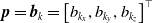 $\boldsymbol{{p}} = \boldsymbol{{b}}_k=\left [b_{k_x}, b_{k_y}, b_{k_z}\right ]^\top$
,
$\boldsymbol{{p}} = \boldsymbol{{b}}_k=\left [b_{k_x}, b_{k_y}, b_{k_z}\right ]^\top$
,
 $\theta _x ={\alpha }_k,\, \theta _y = \beta _k,$
and
$\theta _x ={\alpha }_k,\, \theta _y = \beta _k,$
and
 $\theta _z = \gamma _k$
.
$\theta _z = \gamma _k$
.
B. Collision model for a cuboid moving platform
The two case studies of
 $4$
-
$4$
-
 $4$
CDPR reported in Section 4.2 need restriction of the vertical motion of a cuboid MP to resemble its contactFootnote
6
with the ground. Therefore, if and when the bottom side of the MP touches the ground, that is,
$4$
CDPR reported in Section 4.2 need restriction of the vertical motion of a cuboid MP to resemble its contactFootnote
6
with the ground. Therefore, if and when the bottom side of the MP touches the ground, that is,
 $\xi _z = \frac{{h_{\textrm{m}}}}{2}$
, an additional SDE along the
$\xi _z = \frac{{h_{\textrm{m}}}}{2}$
, an additional SDE along the
 $Z_0$
-axis is attached to its centre of mass
$Z_0$
-axis is attached to its centre of mass
 ${\boldsymbol{\xi }_{\textrm{c}}}={\left [\xi _x, \xi _y, \xi _z\right ]}^\top$
, where the symbol
${\boldsymbol{\xi }_{\textrm{c}}}={\left [\xi _x, \xi _y, \xi _z\right ]}^\top$
, where the symbol
 $h_{\textrm{m}}$
denotes the height of the MP. The associated changes in modelling the MP with contact (Case A) and without contact (Case B) are depicted in Fig. 35.
$h_{\textrm{m}}$
denotes the height of the MP. The associated changes in modelling the MP with contact (Case A) and without contact (Case B) are depicted in Fig. 35.
Changes in the model of the cuboid MP of
 $4$
-
$4$
-
 $4$
CDPR based on its state of contact with the ground. Case A is used when it is in contact with the ground and case B when it is not in contact. The symbol
$4$
CDPR based on its state of contact with the ground. Case A is used when it is in contact with the ground and case B when it is not in contact. The symbol
 $\xi _z$
represents the vertical position of the centre of mass of the MP with respect to the frame
$\xi _z$
represents the vertical position of the centre of mass of the MP with respect to the frame
 $\boldsymbol{{o}}$
-
$\boldsymbol{{o}}$
-
 $X_0Y_0Z_0$
.
$X_0Y_0Z_0$
.

Consequently, the external forces acting on the MP are updated to
 $\boldsymbol{\tau }_5={\left [0,0,F_z,0,0,0\right ]}^\top$
, where
$\boldsymbol{\tau }_5={\left [0,0,F_z,0,0,0\right ]}^\top$
, where
 \begin{align} F_z = \left \{ \begin{array}{l@{\quad}l} 0, &{\xi _{\textrm{z}}} \gt \dfrac{{h_{\textrm{m}}}}{2}\\[10pt]{s_{\textrm{g}}} \left (\xi _z-\dfrac{{h_{\textrm{m}}}}{2}\right ) +{d_{\textrm{g}}} \dot{\xi }_z, &{\xi _{\textrm{z}}} \leq \dfrac{{h_{\textrm{m}}}}{2}. \end{array}\right . \end{align}
In Eq. (B1), the symbols
 $s_{\textrm{g}}$
and
$s_{\textrm{g}}$
and
 $d_{\textrm{g}}$
denote the coefficients of stiffness and damping of the additional SDE. The numerical valuesFootnote
7
of these parameters used in the simulations of the
$d_{\textrm{g}}$
denote the coefficients of stiffness and damping of the additional SDE. The numerical valuesFootnote
7
of these parameters used in the simulations of the
 $4$
-
$4$
-
 $4$
CDPR are
$4$
CDPR are
 ${s_{\textrm{g}}}=10^3$
N/m and
${s_{\textrm{g}}}=10^3$
N/m and
 ${d_{\textrm{g}}}=10^2$
Ns/m.
${d_{\textrm{g}}}=10^2$
Ns/m.
C. Numerical data used for the simulation of the 4-4 cable-driven parallel robot
The values of the geometric parameters, inertia properties of the cables and the MP are adopted from the work of [Reference Goodarzi and Lee20]. Since the elastic and damping properties of the cables are not included in their work, the material properties of the cables are selected from the experimental results presented in ref. [Reference Baklouti, Courteille, Caro and Dkhil41]. The numerical values of these parameters are listed in Table II. The notations used for representing the architecture of the robot are as per the outline given in Section 4.1.
Numerical values of the architecture parameters, inertia properties and material constants used in the dynamic analysis of the
 $4$
-
$4$
-
 $4$
cable-driven parallel robot.
$4$
cable-driven parallel robot.

D. Numerical data used for the simulation of quadcopters
The numerical values listed in Table III correspond to the quadcopter built at the Flight Dynamics and Control Lab, Department of Mechanical and Aerospace Engineering, The George Washington University. A description of its hardware was reported in [Reference Goodarzi, Lee and Lee42].
Numerical values of the architecture parameters and inertia properties of the quadcopters.

E. Indices used for the validation of simulation results
The ODE solver ode15s is only used to guarantee the satisfaction of the indexFootnote 8 1 differential-algebraic equations (DAEs), that is, Eq. (1) and Eq. (5), to be within desired tolerances. Therefore, the satisfaction of the constraint equations and their derivatives, given by Eq. (3) and Eq. (4), respectively, are explicitly verified for all the simulations reported in this work. Further, the agreement of the additional scleronomic and rheonomic constraint functions in Eq. (9) and Eq. (10), respectively, for accurate incorporation of the desired Type II actuation is confirmed.
The evolution of the configuration
 $\boldsymbol{{q}}(t)$
is verified to be consistent with the constraint functions
$\boldsymbol{{q}}(t)$
is verified to be consistent with the constraint functions
 $\boldsymbol{\eta }={\left [\eta _1,\dots, \eta _8\right ]}^\top$
by computing the norm of their residues, denoted by
$\boldsymbol{\eta }={\left [\eta _1,\dots, \eta _8\right ]}^\top$
by computing the norm of their residues, denoted by
 $e_1$
:
$e_1$
:
 \begin{align} e_1 ={\| \boldsymbol{\eta }(\boldsymbol{{q}}, t)\|}_2, \end{align}
where
 ${\| \cdot \|}_2$
denotes the
${\| \cdot \|}_2$
denotes the
 $L^2$
norm of a vector. Similarly, the conformance of the combined evolution of the configuration
$L^2$
norm of a vector. Similarly, the conformance of the combined evolution of the configuration
 $\boldsymbol{{q}}(t)$
and its change
$\boldsymbol{{q}}(t)$
and its change
 ${\dot{\boldsymbol{{q}}}}(t)$
are ratified by finding the norm of the residues of derivatives of the constraint functions, represented by
${\dot{\boldsymbol{{q}}}}(t)$
are ratified by finding the norm of the residues of derivatives of the constraint functions, represented by
 $e_2$
:
$e_2$
:
 \begin{align} e_2 ={\| \dot{\boldsymbol{\eta }}(\boldsymbol{{q}},{\dot{\boldsymbol{{q}}}}, t)\|}_2. \end{align}
The minimal values of the errors
 $e_1$
and
$e_1$
and
 $e_2$
indicate that the dynamic evolution of the robot is consistent with the fundamental laws of mechanics, that is, index 3 DAE, given by, Eq. (1) or Eq. (6), Eq. (3), and Eq. (9) or Eq. (10).
$e_2$
indicate that the dynamic evolution of the robot is consistent with the fundamental laws of mechanics, that is, index 3 DAE, given by, Eq. (1) or Eq. (6), Eq. (3), and Eq. (9) or Eq. (10).


 Open access