


1. Introduction
While turbulence often appears random, many turbulent flows contain underlying structures, such as eddies and vortices. The scale and nature of these structures vary depending on the flow conditions. Identifying these structures allows for a more detailed description of the flow, as well as the isolation of the dominant structures within the turbulence based on their contribution to the quantity or phenomenon of interest, such as turbulent kinetic energy (TKE) or mixing. Ranking these structures based on their significance to a given application or study allows the construction of parsimonious reduced-order models, which can be used to reduce the computational intensity of analyses or to reduce noise from experimental data.
The complex flow phenomena present in the flow over bluff bodies, even at low Reynolds numbers, develop with increasing Reynolds number, and remain a subject of ongoing study. In this respect, the flow over spheres serves as a canonical model for flows over axisymmetric bluff bodies, and is of particular interest for advancing the understanding of these flow phenomena. The phenomena observed in the wake of a sphere include transition from axisymmetry to planar symmetry, from planar symmetry to asymmetry, the formation and shedding of vortices, the development of shear layer instabilities and flow separation. As the flow over a sphere varies significantly with Reynolds number, experimental and numerical investigations have explored a wide range of Reynolds number regimes.
In the context of experimental studies of the flow over spheres, one of the main challenges is fixing the sphere in a wind or water tunnel test section with minimal disturbance of the flow, since the mounting and support structure of the sphere frequently has a significant influence on the flow. The supports chosen for an experiment should simultaneously provide rigid and stable positioning of the sphere, and minimise the disturbance to the flow, while facilitating probe placement and maintaining unobstructed optical access for measurements. Some of the supports used in these studies include rigid downstream supports (Achenbach Reference Achenbach1972), honeycomb structures with rigid supports upstream of the sphere (Grandemange, Gohlke & Cadot Reference Grandemange, Gohlke and Cadot2014; Muyshondt et al. Reference Muyshondt, Nguyen, Hassan and Anand2021) and wires arranged azimuthally (Sakamoto & Haniu Reference Sakamoto and Haniu1990; Jang & Lee Reference Jang and Lee2008). The drag on the spheres has been measured using hot-wire probes (Achenbach Reference Achenbach1972; Tyagi et al. Reference Tyagi, Liu, Ting and Johnston2006), with flow visualisations performed using aluminium dust (Taneda Reference Taneda1956), smoke (Taneda Reference Taneda1978; Jang & Lee Reference Jang and Lee2008) and dyes (Achenbach Reference Achenbach1974; Sakamoto & Haniu Reference Sakamoto and Haniu1990; Johnson & Patel Reference Johnson and Patel1999) to provide a qualitative understanding of the recirculation region, flow separation and vortex shedding in the wake. Various forms of particle image velocimetry (PIV), including planar (Jang & Lee Reference Jang and Lee2008), stereoscopic (Muyshondt et al. Reference Muyshondt, Nguyen, Hassan and Anand2021) and tomographic (David et al. Reference David, Eshbal, Rinsky and van Hout2020), have been used to quantitatively measure the flow around spheres.
While mounting the sphere is not a concern in numerical studies, simulations are subject to distinct challenges. The problem geometry and the wide range of scales involved require careful consideration of the mesh and solver to accurately resolve the flow at high Reynolds numbers. Because of this complexity, large eddy simulation (LES) (Tomboulides, Orszag & Karniadakis Reference Tomboulides, Orszag and Karniadakis1993; Tomboulides & Orszag Reference Tomboulides and Orszag2000; Constantinescu & Squires Reference Constantinescu and Squires2003; Rodriguez et al. Reference Rodriguez, Borell, Lehmkuhl, Segarra and Oliva2011) and detached eddy simulation (DES) (Constantinescu & Squires Reference Constantinescu and Squires2003, Reference Constantinescu and Squires2004) methods have been preferred over the more computationally expensive direct numerical simulation (DNS) (Tomboulides et al. Reference Tomboulides, Orszag and Karniadakis1993; Rodriguez et al. Reference Rodriguez, Borell, Lehmkuhl, Segarra and Oliva2011; Rodríguez et al. Reference Rodríguez, Lehmkuhl, Borrell and Oliva2013; Rodriguez et al. Reference Rodriguez, Lehmkuhl, Soria, Gómez, Domínguez-Pumar and Kowalski2019) for resolving the primary features of the flow at high Reynolds numbers. In conjunction with the advancement of computational capabilities, these models have expanded the scope of numerical investigations of the flow over spheres to large Reynolds numbers.
Experimental and numerical studies have examined the development of the flow over spheres over a wide range of Reynolds number regimes. At low Reynolds number, $Re_D \lt 20$
, the flow in the wake is laminar and axisymmetric, and recirculation is absent (Taneda Reference Taneda1956; Tomboulides & Orszag Reference Tomboulides and Orszag2000). A small vortex ring forms near the rear stagnation point around
$Re_D \lt 20$
, the flow in the wake is laminar and axisymmetric, and recirculation is absent (Taneda Reference Taneda1956; Tomboulides & Orszag Reference Tomboulides and Orszag2000). A small vortex ring forms near the rear stagnation point around $Re_D \approx 25$
(Taneda Reference Taneda1956), and elongates in the streamwise direction with increasing Reynolds number. This vortex ring begins to oscillate around
$Re_D \approx 25$
(Taneda Reference Taneda1956), and elongates in the streamwise direction with increasing Reynolds number. This vortex ring begins to oscillate around $Re_D \approx 130$
with a long period, which becomes more prominent at higher Reynolds numbers. The recirculation region formed behind the sphere, which exhibits reverse flow in the mean flow, extends further downstream of the sphere as Reynolds number increases (Johnson & Patel Reference Johnson and Patel1999).
$Re_D \approx 130$
with a long period, which becomes more prominent at higher Reynolds numbers. The recirculation region formed behind the sphere, which exhibits reverse flow in the mean flow, extends further downstream of the sphere as Reynolds number increases (Johnson & Patel Reference Johnson and Patel1999).
The axisymmetry in the wake at low Reynolds number is lost due to the formation of a double-threaded wake around $Re_D \approx 210$
(Johnson & Patel Reference Johnson and Patel1999; Tomboulides & Orszag Reference Tomboulides and Orszag2000), which consists of two streamwise vortices of opposite sign that can be seen as dye threads in the wake of a free-falling sphere (Magarvey & MacLatchy Reference Magarvey and MacLatchy1965). Single-frequency vortex shedding begins around
$Re_D \approx 210$
(Johnson & Patel Reference Johnson and Patel1999; Tomboulides & Orszag Reference Tomboulides and Orszag2000), which consists of two streamwise vortices of opposite sign that can be seen as dye threads in the wake of a free-falling sphere (Magarvey & MacLatchy Reference Magarvey and MacLatchy1965). Single-frequency vortex shedding begins around $Re_D \approx 300$
(Taneda Reference Taneda1956; Sakamoto & Haniu Reference Sakamoto and Haniu1990), and hairpin-shaped vortices form at
$Re_D \approx 300$
(Taneda Reference Taneda1956; Sakamoto & Haniu Reference Sakamoto and Haniu1990), and hairpin-shaped vortices form at $Re_D \approx 400$
(Achenbach Reference Achenbach1974). The generation of an unsteady random side force, which has been observed in both experimental (Taneda Reference Taneda1978) and numerical (Yun, Kim & Choi Reference Yun, Kim and Choi2006) studies, leads to the loss of planar symmetry in the wake within the range of
$Re_D \approx 400$
(Achenbach Reference Achenbach1974). The generation of an unsteady random side force, which has been observed in both experimental (Taneda Reference Taneda1978) and numerical (Yun, Kim & Choi Reference Yun, Kim and Choi2006) studies, leads to the loss of planar symmetry in the wake within the range of $400 \lt Re_D \lt 500$
(Taneda Reference Taneda1956).
$400 \lt Re_D \lt 500$
(Taneda Reference Taneda1956).
For $Re_D \gtrapprox 800$
, the small-scale Kelvin–Helmholtz instability in the shear layer at the edge of the recirculation region appears as axisymmetric vortex shedding (Chomaz, Bonneton & Hopfinger Reference Chomaz, Bonneton and Hopfinger1993; Constantinescu & Squires Reference Constantinescu and Squires2004). This is the higher frequency of two instability modes identified in the wake of the sphere by Kim & Durbin (Reference Kim and Durbin1988), with the lower-frequency mode arising from large-scale vortex shedding. Small-scale vortical structures are shed from the main vortical structure around
$Re_D \gtrapprox 800$
, the small-scale Kelvin–Helmholtz instability in the shear layer at the edge of the recirculation region appears as axisymmetric vortex shedding (Chomaz, Bonneton & Hopfinger Reference Chomaz, Bonneton and Hopfinger1993; Constantinescu & Squires Reference Constantinescu and Squires2004). This is the higher frequency of two instability modes identified in the wake of the sphere by Kim & Durbin (Reference Kim and Durbin1988), with the lower-frequency mode arising from large-scale vortex shedding. Small-scale vortical structures are shed from the main vortical structure around $Re_D \approx 1000$
(Yun et al. Reference Yun, Kim and Choi2006), and the recirculation region behind the sphere begins to shrink with increasing Reynolds number. Periodic fluctuations are present in the wake for significantly higher Reynolds numbers,
$Re_D \approx 1000$
(Yun et al. Reference Yun, Kim and Choi2006), and the recirculation region behind the sphere begins to shrink with increasing Reynolds number. Periodic fluctuations are present in the wake for significantly higher Reynolds numbers, $Re_D = O(10^6)$
(Achenbach Reference Achenbach1974).
$Re_D = O(10^6)$
(Achenbach Reference Achenbach1974).
Since its first application to turbulent flows by Lumley (Reference Lumley1967), proper orthogonal decomposition (POD) has been widely used for identifying and analysing structures in turbulence (Sirovich Reference Sirovich1987; Berkooz, Holmes & Lumley Reference Berkooz, Holmes and Lumley1993). As POD does not require temporal resolution of the flow and can thus be applied to non-time-resolved data, it is a robust yet straightforward method for identifying the structures within a turbulent flow. In the case of the flow over a cylinder, the turbulent fluctuations due to the vortices shed from the cylinder can be identified in the leading POD modes (Oudheusden et al. Reference Oudheusden, Scarano, Hinsberg and Watt2005; Perrin et al. Reference Perrin, Cid, Cazin, Sevrain, Braza, Moradei and Harran2007b ). The energy of these modes is significantly larger than the higher-order modes, and their phase angle is clearly related to that of the pressure fluctuations resulting from the shed vortices (Perrin et al. Reference Perrin, Braza, Cid, Cazin, Barthet, Sevrain, Mockett and Thiele2007a ). Similarly, periodic structures in screeching, impinging and free jets (Edgington-Mitchell et al. Reference Edgington-Mitchell, Oberleithner, Honnery and Soria2014; Weightman et al. Reference Weightman, Amili, Honnery, Soria and Edgington-Mitchell2017, Reference Weightman, Amili, Honnery, Soria and Edgington-Mitchell2018) are represented by the leading POD modes. Identifying pairs of POD modes which represent periodic structures enables the a posteriori phase averaging of experimental data collected asynchronously or at a low sampling frequency relative to these structures. However, the complexity of the flow over a sphere in this regime makes identification of periodic structures in the turbulent fluctuations challenging, as POD modes representing different phases of a structure are not inherently linked by the decomposition.
The analytic signal of the turbulent fluctuations, which is defined using the Hilbert transform, can be decomposed into complex modes that include phase information using POD (Horel Reference Horel1984). While the Hilbert transform is performed in time for time-resolved data, it can also be performed in an analogous spatial direction when the data are not time resolved (Kriegseis et al. Reference Kriegseis, Kinzel and Nobach2021; Raiola & Kriegseis Reference Raiola and Kriegseis2024a , Reference Raiola and Kriegseisb ). This results in modes emphasising structures which are periodic in the chosen direction, with the streamwise direction being the most appropriate choice to identify structures which propagate downstream from the sphere. Although a useful method for identifying propagating structures, Hilbert POD (HPOD) introduces spectral leakage to the modes due to the Hilbert transform being derived from the Fourier transform, which inherently assumes periodicity.
Raiola & Kriegseis (Reference Raiola and Kriegseis2025) demonstrated the ability of spatial HPOD to extract spatiotemporally coherent wavepackets from flows with significant advecting structures. Their application of HPOD to DNS of a laminar vortex street in the wake of a cylinder at $Re_D = 100$
showed that the spatial HPOD provides a more compact decomposition than POD. In this case, the first two POD modes representing the vortex street were captured by a single HPOD mode. In this example, the leading mode of the spatial HPOD was able to capture the first two POD modes even when the data were shuffled in time and the dataset reduced in size, whereas the modes of the conventional time-based HPOD converged towards the POD modes, and no longer captured paired POD modes in a single HPOD mode. They further applied HPOD to LES of a turbulent jet at
$Re_D = 100$
showed that the spatial HPOD provides a more compact decomposition than POD. In this case, the first two POD modes representing the vortex street were captured by a single HPOD mode. In this example, the leading mode of the spatial HPOD was able to capture the first two POD modes even when the data were shuffled in time and the dataset reduced in size, whereas the modes of the conventional time-based HPOD converged towards the POD modes, and no longer captured paired POD modes in a single HPOD mode. They further applied HPOD to LES of a turbulent jet at $Re_D = 10^6$
(Towne et al. Reference Towne2023), showing that the spatial HPOD could still identify advecting wavepackets in a flow with a broader range of scales. Finally, HPOD was applied to PIV data from a turbulent subsonic jet (Raiola & Ragni Reference Raiola and Ragni2019) at
$Re_D = 10^6$
(Towne et al. Reference Towne2023), showing that the spatial HPOD could still identify advecting wavepackets in a flow with a broader range of scales. Finally, HPOD was applied to PIV data from a turbulent subsonic jet (Raiola & Ragni Reference Raiola and Ragni2019) at $Re = 33\,000$
, which lacked the temporal resolution afforded by the LES data. Despite this limitation, the spatial HPOD was able to extract spatial modes similar to those identified in the LES data.
$Re = 33\,000$
, which lacked the temporal resolution afforded by the LES data. Despite this limitation, the spatial HPOD was able to extract spatial modes similar to those identified in the LES data.
The current work applies both POD and HPOD, with the Hilbert transform performed in the streamwise direction following the methodology of Raiola & Kriegseis (Reference Raiola and Kriegseis2025), to experimentally measured velocity fluctuations in the wake of a sphere at $Re_D = 7780$
. Modes resulting from each decomposition are compared, and correlations between the POD and HPOD modes are used to identify POD mode pairs representing propagating structures. A novel approach is introduced in which the Hilbert transform is applied directly to the POD modes, allowing mode pairs associated with periodic or propagating structures to be identified without performing POD on the complex analytic signal of the turbulent fluctuations. This method significantly reduces the computational cost of identifying propagating structures and preserves the energy ranking of the modes relative to the original data. The identified POD mode pairs are then used to phase average the velocity fluctuations in the wake of the sphere to examine the propagating structures, while phase-averaging based on HPOD modes is also performed to demonstrate the influence of HPOD on the identified structures due to its emphasis on propagating structures and inherent assumption of periodicity.
$Re_D = 7780$
. Modes resulting from each decomposition are compared, and correlations between the POD and HPOD modes are used to identify POD mode pairs representing propagating structures. A novel approach is introduced in which the Hilbert transform is applied directly to the POD modes, allowing mode pairs associated with periodic or propagating structures to be identified without performing POD on the complex analytic signal of the turbulent fluctuations. This method significantly reduces the computational cost of identifying propagating structures and preserves the energy ranking of the modes relative to the original data. The identified POD mode pairs are then used to phase average the velocity fluctuations in the wake of the sphere to examine the propagating structures, while phase-averaging based on HPOD modes is also performed to demonstrate the influence of HPOD on the identified structures due to its emphasis on propagating structures and inherent assumption of periodicity.
Section 2 outlines the theoretical aspects of POD and HPOD and the rationale for applying the Hilbert transform directly to the POD modes. Section 3 provides details of the experimental facility and measurement methodology. Section 4 presents the analysis and results of the POD and HPOD, the pairing of POD modes using HPOD modes, the application of the Hilbert transform directly to the POD modes and the resulting phase averages of the turbulent fluctuations. Section 5 summarises the work, highlights the key findings, and provides closing remarks.
2. Theoretical considerations
2.1. Proper orthogonal decomposition
Proper orthogonal decomposition decomposes statistically independent snapshots of the random field $\boldsymbol{f}(\boldsymbol{x},t)$
into orthonormal spatial modes
$\boldsymbol{f}(\boldsymbol{x},t)$
into orthonormal spatial modes $\psi _k(\boldsymbol{x})$
with temporal coefficients
$\psi _k(\boldsymbol{x})$
with temporal coefficients $a_k(t)$
, which are ranked by their associated energy
$a_k(t)$
, which are ranked by their associated energy $\lambda _k$
in descending order, such that
$\lambda _k$
in descending order, such that
 \begin{equation} \boldsymbol{f}(\boldsymbol{x},t) = \sum _{k=1}^{K} a_k(t)\psi _k(\boldsymbol{x}), \end{equation}
and is mathematically analogous to singular value decomposition and principal component analysis. In the application of POD to turbulence, $\boldsymbol{f}(\boldsymbol{x},t)$
represents the turbulent fluctuations, and
$\boldsymbol{f}(\boldsymbol{x},t)$
represents the turbulent fluctuations, and $\lambda _k$
represents the contribution of the
$\lambda _k$
represents the contribution of the $k^{}$
th mode to the total TKE of
$k^{}$
th mode to the total TKE of $\boldsymbol{f}(\boldsymbol{x},t)$
. A common use for POD is the definition of a reduced-order representation of
$\boldsymbol{f}(\boldsymbol{x},t)$
. A common use for POD is the definition of a reduced-order representation of $\boldsymbol{f}(\boldsymbol{x},t)$
by reconstructing the original data using
$\boldsymbol{f}(\boldsymbol{x},t)$
by reconstructing the original data using $\hat {K} \lt K$
modes
$\hat {K} \lt K$
modes
 \begin{equation} \hat {\boldsymbol{f}}(\boldsymbol{x},t) = \sum _{k=1}^{\hat {K}} a_k(t)\psi _k(\boldsymbol{x}), \end{equation}
which represents a portion of the total kinetic energy equal to
 \begin{equation} \textrm{TKE} = 100 \times \frac {\sum _{k=1}^{\hat {K}}\lambda _k}{\sum _{k=1}^{K}\lambda _k} \ \%. \end{equation}
In order to perform POD, the two-point correlation of $\boldsymbol{f}(\boldsymbol{x},t)$
in space
$\boldsymbol{f}(\boldsymbol{x},t)$
in space
 \begin{equation} C(\boldsymbol{x},\boldsymbol{x}') = \int _{T} \boldsymbol{f}(\boldsymbol{x},t) \boldsymbol{f}(\boldsymbol{x}',t) \, {\rm d}t, \end{equation}
is calculated, where $T$
denotes the temporal domain. The spatial modes and the corresponding energy are given by the eigendecomposition of
$T$
denotes the temporal domain. The spatial modes and the corresponding energy are given by the eigendecomposition of $C(\boldsymbol{x},\boldsymbol{x}')$
 \begin{equation} \int _S C(\boldsymbol{x},\boldsymbol{x}') \psi (\boldsymbol{x}') \, {\rm d}\boldsymbol{x}'= \lambda \psi (\boldsymbol{x}), \end{equation}
where $S$
denotes the spatial domain. The temporal coefficients are computed by projecting
$S$
denotes the spatial domain. The temporal coefficients are computed by projecting $\boldsymbol{f}(\boldsymbol{x},t)$
onto
$\boldsymbol{f}(\boldsymbol{x},t)$
onto $\psi (\boldsymbol{x})$
 \begin{equation} a(t) = \int _S \boldsymbol{f}(\boldsymbol{x},t)\psi (\boldsymbol{x}) \, {\rm d}\boldsymbol{x}. \end{equation}
Alternatively, POD can be implemented using the method of snapshots, which first computes the temporal coefficients, and subsequently determines the spatial modes. This approach is more computationally efficient when the number of spatial coordinates in $\boldsymbol{f}(\boldsymbol{x},t)$
exceeds the number of realisations of the field. The two-instant temporal correlation
$\boldsymbol{f}(\boldsymbol{x},t)$
exceeds the number of realisations of the field. The two-instant temporal correlation
 \begin{equation} C(t,t') = \int _{S} \boldsymbol{f}(\boldsymbol{x},t) \boldsymbol{f}(\boldsymbol{x},t') \, {\rm d}\boldsymbol{x}, \end{equation}
is used instead of the spatial correlation defined in (2.4). The eigendecomposition of $C(t,t')$
 \begin{equation} \int _T C(t,t') a(t') \, {\rm d}t'= \lambda a(t), \end{equation}
yields the eigenvalues and corresponding temporal coefficients. The spatial modes are subsequently obtained by projecting $\boldsymbol{f}(\boldsymbol{x},t)$
onto
$\boldsymbol{f}(\boldsymbol{x},t)$
onto $a(t)$
 \begin{equation} \psi (\boldsymbol{x})= \int _T \boldsymbol{f}(\boldsymbol{x},t)a(t) \, {\rm d}t. \end{equation}
When the $i^{}$
th and
$i^{}$
th and $j^{}$
th POD modes represent the same periodic structure separated in phase by
$j^{}$
th POD modes represent the same periodic structure separated in phase by $\pm \pi /2$
, their temporal coefficients can be expressed as functions of the phase angle
$\pm \pi /2$
, their temporal coefficients can be expressed as functions of the phase angle $\phi _{i,j}$
of the structure as
$\phi _{i,j}$
of the structure as
 \begin{equation} a_i(t) = \sqrt {2 \lambda _i}\cos (\phi _{i,j}(t)), \end{equation}
and
 \begin{equation} a_j(t) = \sqrt {2 \lambda _j}\sin (\phi _{i,j}(t)), \end{equation}
respectively. Consequently, the phase angle $\phi _{i,j}(t)$
is given by
$\phi _{i,j}(t)$
is given by
 \begin{equation} \phi _{i,j}(t) = \tan ^{-1} \left ( \frac {a_j(t)/\sqrt {2 \lambda _j}}{a_i(t)/\sqrt {2 \lambda _i}} \right )\!. \end{equation}
The phase-averaged representation of the data using the $i^{}$
th and
$i^{}$
th and $j^{}$
th POD modes at the phase angle
$j^{}$
th POD modes at the phase angle $\phi$
is defined as
$\phi$
is defined as
 \begin{equation} \widetilde {\boldsymbol{f}}(\boldsymbol{x},\phi ) = \sum _{k=1}^K a_k(t) \psi _k(\boldsymbol{x}) \, | \, \phi _{i,j}(t)=\phi ,\end{equation}
where $\phi _{i,j}(t)$
is defined by (2.12). Although any two POD modes can be employed for phase-averaging
$\phi _{i,j}(t)$
is defined by (2.12). Although any two POD modes can be employed for phase-averaging $\boldsymbol{f}(\boldsymbol{x},t)$
, not all mode selections yield physically meaningful phase averages. For strongly dominant periodic fluctuations, the temporal coefficients of the corresponding modes exhibit a circular distribution in the coefficient space (Oudheusden et al. Reference Oudheusden, Scarano, Hinsberg and Watt2005). Large-scale periodic structures can also be identified by comparing the phase angle of the modes with an independent phase measurement of the flow, such as pressure signals (Perrin et al. Reference Perrin, Braza, Cid, Cazin, Barthet, Sevrain, Mockett and Thiele2007a
). However, as periodic structures become less prominent, establishing a clear relationship between the corresponding POD modes becomes increasingly challenging.
$\boldsymbol{f}(\boldsymbol{x},t)$
, not all mode selections yield physically meaningful phase averages. For strongly dominant periodic fluctuations, the temporal coefficients of the corresponding modes exhibit a circular distribution in the coefficient space (Oudheusden et al. Reference Oudheusden, Scarano, Hinsberg and Watt2005). Large-scale periodic structures can also be identified by comparing the phase angle of the modes with an independent phase measurement of the flow, such as pressure signals (Perrin et al. Reference Perrin, Braza, Cid, Cazin, Barthet, Sevrain, Mockett and Thiele2007a
). However, as periodic structures become less prominent, establishing a clear relationship between the corresponding POD modes becomes increasingly challenging.
2.2. Hilbert proper orthogonal decomposition
Hilbert proper orthogonal decomposition incorporates phase information into the modes by replacing $\boldsymbol{f}(\boldsymbol{x},t)$
with its analytic signal (Horel Reference Horel1984)
$\boldsymbol{f}(\boldsymbol{x},t)$
with its analytic signal (Horel Reference Horel1984)
 \begin{equation} \boldsymbol{f}^a(\boldsymbol{x},t) = \boldsymbol{f}(\boldsymbol{x},t) + i \mathcal{H}[\boldsymbol{f}(\boldsymbol{x},t)], \end{equation}
where $\mathcal{H}$
denotes the Hilbert transform of
$\mathcal{H}$
denotes the Hilbert transform of $\boldsymbol{f}(\boldsymbol{x},t)$
with respect to time
$\boldsymbol{f}(\boldsymbol{x},t)$
with respect to time
 \begin{equation} \mathcal{H}\big [ \boldsymbol{f}(\boldsymbol{x},t) \big ] = \frac {1}{\pi } \int _{-\infty }^{\infty } \frac {\boldsymbol{f}(\boldsymbol{x},\tau )}{t-\tau } \, {\rm d}\tau . \end{equation}
The Hilbert transform is equivalent to a $\mp \pi /2$
phase shift of the fundamental frequency components of
$\mp \pi /2$
phase shift of the fundamental frequency components of $\boldsymbol{f}(\boldsymbol{x},t)$
in Fourier space (Thomas Reference Thomas1969)
$\boldsymbol{f}(\boldsymbol{x},t)$
in Fourier space (Thomas Reference Thomas1969)
 \begin{equation} \mathcal{H}\big [ \boldsymbol{f}(\boldsymbol{x},t) \big ] = \mathcal{F}^{-1}\big [-i \textrm {sgn}(f) \mathcal{F}\big [ \boldsymbol{f}(\boldsymbol{x},t) \big ]\big ], \end{equation}
where $\mathcal{F}$
and
$\mathcal{F}$
and $\mathcal{F}^{-1}$
are the Fourier transform and inverse Fourier transform, respectively, and
$\mathcal{F}^{-1}$
are the Fourier transform and inverse Fourier transform, respectively, and
 \begin{equation} \textrm {sgn}(f) = \begin{cases} -1 & \text{if } f \lt 0,\\ \phantom {-}0 & \text{if } f = 0 ,\\ \phantom {-}1 & \text{if } f \gt 0 ,\\ \end{cases} \end{equation}
is the sign of the instantaneous frequency $f$
of each term in the Fourier series given by
$f$
of each term in the Fourier series given by $\mathcal{F} [\boldsymbol{f}(\boldsymbol{x},t) ]$
.
$\mathcal{F} [\boldsymbol{f}(\boldsymbol{x},t) ]$
.
For time-resolved data, the Hilbert transform is applied with respect to time to compute the analytic signal $\boldsymbol{f}^{a}(\boldsymbol{x},t)$
. The HPOD is implemented on time-resolved data by substituting
$\boldsymbol{f}^{a}(\boldsymbol{x},t)$
. The HPOD is implemented on time-resolved data by substituting $\boldsymbol{f}(\boldsymbol{x},t)$
in (2.4) to (2.6) with its analytic signal. For flows where coherent structures propagate downstream, the Hilbert transform can alternatively be applied in the streamwise direction
$\boldsymbol{f}(\boldsymbol{x},t)$
in (2.4) to (2.6) with its analytic signal. For flows where coherent structures propagate downstream, the Hilbert transform can alternatively be applied in the streamwise direction
 \begin{equation} \mathcal{H}_{x} \big [ \boldsymbol{f}(\boldsymbol{x},t) \big ] = \frac {1}{\pi } \int _{-\infty }^{\infty } \frac {\boldsymbol{f}\big ( (\xi ,\ldots ), t \big )}{x-\xi } \, {\rm d}\xi . \end{equation}
This approach uses streamwise propagation as an analogue for temporal evolution, allowing the method to be applied to data that are not time resolved (Kriegseis et al. Reference Kriegseis, Kinzel and Nobach2021; Raiola & Kriegseis Reference Raiola and Kriegseis2024a , Reference Raiola and Kriegseisb ).
In this case, the analytic signal of $\boldsymbol{f}(\boldsymbol{x},t)$
is defined using the streamwise Hilbert transform
$\boldsymbol{f}(\boldsymbol{x},t)$
is defined using the streamwise Hilbert transform $\mathcal{H}_x$
 \begin{equation} \boldsymbol{f}^a_x (\boldsymbol{x},t) = \boldsymbol{f}(\boldsymbol{x},t) + i \mathcal{H}_{x} \big [ \boldsymbol{f}(\boldsymbol{x},t) \big ], \end{equation}
and is substituted for $\boldsymbol{f}(\boldsymbol{x},t)$
in (2.7) to (2.9). The resulting eigenvalues
$\boldsymbol{f}(\boldsymbol{x},t)$
in (2.7) to (2.9). The resulting eigenvalues $\lambda ^a_k$
represent the contribution of the
$\lambda ^a_k$
represent the contribution of the $k^{}$
th mode to the total TKE of the analytic signal and are real valued. The spatial modes
$k^{}$
th mode to the total TKE of the analytic signal and are real valued. The spatial modes $\psi ^a_k(\boldsymbol{x})$
are complex, with the imaginary component of
$\psi ^a_k(\boldsymbol{x})$
are complex, with the imaginary component of $\psi ^a_k(\boldsymbol{x})$
corresponding to a
$\psi ^a_k(\boldsymbol{x})$
corresponding to a $\mp \pi /2$
phase shift of the real component.
$\mp \pi /2$
phase shift of the real component.
The instantaneous amplitude and phase angle of the $k^{}$
th mode are defined by the real
$k^{}$
th mode are defined by the real $\textrm{Re}$
and imaginary
$\textrm{Re}$
and imaginary $\textrm{Im}$
components of
$\textrm{Im}$
components of $a^a_k(t)$
as
$a^a_k(t)$
as
 \begin{equation} |a^a_k(t)| = \sqrt {\textrm{Re}\, {\big (a^a_k(t)\big )}^2 + \textrm{Im}\, {\big (a^a_k(t)\big )}^2 }, \end{equation}
and
 \begin{equation} \phi ^a_k(t) = \tan ^{-1} \left ( \mp \frac {\textrm{Im}\, \big (a^a_k(t)\big )} {\textrm{Re}\, \big (a^a_k(t)\big )} \right )\!, \end{equation}
respectively. The instantaneous amplitude quantifies the strength of the mode at each instant, while the instantaneous phase angle characterises the mode shape, which oscillates between the real and imaginary components of $\psi ^a_k(\boldsymbol{x})$
at
$\psi ^a_k(\boldsymbol{x})$
at $\phi ^a_k(t)=0^\circ$
and
$\phi ^a_k(t)=0^\circ$
and $\phi ^a_k(t)=\mp \pi /2$
, respectively.
$\phi ^a_k(t)=\mp \pi /2$
, respectively.
The analytic signal can be reconstructed using $\hat {K}$
modes as
$\hat {K}$
modes as
 \begin{equation} \hat {\boldsymbol{f}^a} (\boldsymbol{x},t) = \sum _{k=1}^{\hat {K}} a^a_k(t) \psi ^a_k(\boldsymbol{x}), \end{equation}
where the real part is the reduced-order model of $\boldsymbol{f}(\boldsymbol{x},t)$
including the modes which contribute most to the TKE of the analytic signal. This reconstruction favours the propagating components of
$\boldsymbol{f}(\boldsymbol{x},t)$
including the modes which contribute most to the TKE of the analytic signal. This reconstruction favours the propagating components of $\boldsymbol{f}(\boldsymbol{x},t)$
, but introduces spectral leakage into the reconstruction due to the assumption of periodicity inherent to Hilbert transform.
$\boldsymbol{f}(\boldsymbol{x},t)$
, but introduces spectral leakage into the reconstruction due to the assumption of periodicity inherent to Hilbert transform.
2.3. Hilbert transform of POD modes
Although POD modes do not inherently contain temporal information, the streamwise Hilbert transform can be applied directly to each mode. Thus, the analytic signal of the POD mode $\psi _k(\boldsymbol{x})$
is defined as
$\psi _k(\boldsymbol{x})$
is defined as
 \begin{equation} {(\psi _k)}^a(\boldsymbol{x}) = \psi _k(\boldsymbol{x}) + i\mathcal{H}_x \big [\psi _k(\boldsymbol{x})\big ]. \end{equation}
Substituting the analytic signal of the modes for the POD modes in (2.1) yields
 \begin{equation} \sum _{k=1}^K a_k(t) \Big ( {(\psi _k)}^a(\boldsymbol{x}) \Big ) = \sum _{k=1}^K a_k(t) \Big ( \psi _k(\boldsymbol{x}) + i\mathcal{H}_x \big [ \psi _k(\boldsymbol{x}) \big ] \Big ), \end{equation}
which can be expanded to
 \begin{equation} \sum _{k=1}^K a_k(t) \Big ( {(\psi _k)}^a(\boldsymbol{x}) \Big ) = \sum _{k=1}^K a_k(t) \psi _k(\boldsymbol{x}) + \sum _{k=1}^K a_k(t) i \mathcal{H}_x \big [ \psi _k(\boldsymbol{x}) \big ]. \end{equation}
Since the Hilbert transform is a linear operator, the expression can be rewritten as
 \begin{equation} \begin{aligned} \sum _{k=1}^K a_k(t) \Big ( {(\psi _k)}^a(\boldsymbol{x}) \Big ) & = \sum _{k=1}^K a_k(t)\psi _k(\boldsymbol{x}) + i \mathcal{H}_x \Big [ \sum _{k=1}^K a_k(t)\psi _k(\boldsymbol{x}) \Big ] \\ & = \boldsymbol{f}(\boldsymbol{x},t) + i\mathcal{H}_x[\boldsymbol{f}(\boldsymbol{x},t)] \\ & = \boldsymbol{f}^a_x(\boldsymbol{x},t), \\ \end{aligned} \end{equation}
which is the analytic signal of $\boldsymbol{f}(\boldsymbol{x},t)$
.
$\boldsymbol{f}(\boldsymbol{x},t)$
.
Therefore, applying the Hilbert transform to each POD mode of $\boldsymbol{f}(\boldsymbol{x},t)$
individually and substituting the resulting analytic signals for the original modes enables the reconstruction of
$\boldsymbol{f}(\boldsymbol{x},t)$
individually and substituting the resulting analytic signals for the original modes enables the reconstruction of $\boldsymbol{f}^a(\boldsymbol{x},t)$
. However, the analytic signals of the POD modes are not equal to the HPOD modes, as the decomposition of the analytic signal of
$\boldsymbol{f}^a(\boldsymbol{x},t)$
. However, the analytic signals of the POD modes are not equal to the HPOD modes, as the decomposition of the analytic signal of $\boldsymbol{f}(\boldsymbol{x},t)$
ranks HPOD modes by their energy contribution to
$\boldsymbol{f}(\boldsymbol{x},t)$
ranks HPOD modes by their energy contribution to $\boldsymbol{f}^a(\boldsymbol{x},t)$
rather than to
$\boldsymbol{f}^a(\boldsymbol{x},t)$
rather than to $\boldsymbol{f}(\boldsymbol{x},t)$
. Consequently, leading POD modes may contain non-propagating features that are relegated to higher-order HPOD modes. While this approach is not equivalent to HPOD, the tendency for propagating structures to be decomposed into paired POD modes – or real and imaginary parts of HPOD modes (Raiola & Kriegseis Reference Raiola and Kriegseis2025) – suggests that the Hilbert transform of a POD mode representing a propagating structure should closely match the POD mode corresponding to the
$\boldsymbol{f}(\boldsymbol{x},t)$
. Consequently, leading POD modes may contain non-propagating features that are relegated to higher-order HPOD modes. While this approach is not equivalent to HPOD, the tendency for propagating structures to be decomposed into paired POD modes – or real and imaginary parts of HPOD modes (Raiola & Kriegseis Reference Raiola and Kriegseis2025) – suggests that the Hilbert transform of a POD mode representing a propagating structure should closely match the POD mode corresponding to the $\pi /2$
phase shift of the same structure.
$\pi /2$
phase shift of the same structure.
3. Methodology
3.1. Experimental facility
Experiments were performed in a vertical water tunnel, the test section of which is 1.5 m long with a cross-section of 0.25 m $\times$
0.25 m, shown in figure 1(a) (Buchner & Soria Reference Buchner and Soria2015; Buchner, Honnery & Soria Reference Buchner, Honnery and Soria2017; Davey, Atkinson & Soria Reference Davey, Atkinson and Soria2025). The settling chamber is connected to the top of the test section by a 16:1 contraction, which incorporates a honeycomb and screens to reduce the turbulence intensity and scale in the tunnel test section. Water is pumped from the plenum chamber below the test section up to the settling chamber such that the flow through the test section is downwards. The walls of the test section are made of 15 mm thick clear acrylic. A removable panel is located on one wall for access to the test section, and is set flush to the internal side of the wall to minimise asymmetry in the tunnel. Seeding and filtration of the tunnel is performed via an auxiliary circuit, which is isolated during experiments. A sting of diameter 9.3 mm is mounted to a cross-beam of thin aerofoil cross-sections above the test section. The sting tapers over the last 100 mm to a diameter of 4.65 mm and terminates in a threaded rod used to mount the sphere. A close-up view of the sphere mounting structure is shown in figure 1(b).
$\times$
0.25 m, shown in figure 1(a) (Buchner & Soria Reference Buchner and Soria2015; Buchner, Honnery & Soria Reference Buchner, Honnery and Soria2017; Davey, Atkinson & Soria Reference Davey, Atkinson and Soria2025). The settling chamber is connected to the top of the test section by a 16:1 contraction, which incorporates a honeycomb and screens to reduce the turbulence intensity and scale in the tunnel test section. Water is pumped from the plenum chamber below the test section up to the settling chamber such that the flow through the test section is downwards. The walls of the test section are made of 15 mm thick clear acrylic. A removable panel is located on one wall for access to the test section, and is set flush to the internal side of the wall to minimise asymmetry in the tunnel. Seeding and filtration of the tunnel is performed via an auxiliary circuit, which is isolated during experiments. A sting of diameter 9.3 mm is mounted to a cross-beam of thin aerofoil cross-sections above the test section. The sting tapers over the last 100 mm to a diameter of 4.65 mm and terminates in a threaded rod used to mount the sphere. A close-up view of the sphere mounting structure is shown in figure 1(b).
A sphere with a diameter of $D=40$
mm was fabricated using a Phrozen Sonic Mighty 8k 3D printer, featuring a layer height of 35
$D=40$
mm was fabricated using a Phrozen Sonic Mighty 8k 3D printer, featuring a layer height of 35 $\mathrm{\unicode{x03BC} m}$
and a planar resolution of 22
$\mathrm{\unicode{x03BC} m}$
and a planar resolution of 22 $\mathrm{\unicode{x03BC} m}$ $\times$
22
$\times$
22 $\mathrm{\unicode{x03BC} m}$
, as shown in figure 1(c). The sphere has a shell thickness of 2.5 mm and an external boss at the top for mounting to the threaded rod on the end of the sting. The boss begins parallel to the sting and smoothly transitions to the sphere surface. The sphere is supported internally by a conical structure, which features slits to prevent uncured resin from being trapped in the cavities during printing.
$\mathrm{\unicode{x03BC} m}$
, as shown in figure 1(c). The sphere has a shell thickness of 2.5 mm and an external boss at the top for mounting to the threaded rod on the end of the sting. The boss begins parallel to the sting and smoothly transitions to the sphere surface. The sphere is supported internally by a conical structure, which features slits to prevent uncured resin from being trapped in the cavities during printing.
(a) Vertical water tunnel facility, (b) close-up of the mounting structure and sphere and (c) 3D printed sphere design (Davey et al. Reference Davey, Atkinson and Soria2025).

3.2. Experimental method
Flow measurements in the wake of the sphere were conducted at a free-stream velocity of $U_\infty =200$
mm s−1, corresponding to a Reynolds number of
$U_\infty =200$
mm s−1, corresponding to a Reynolds number of $Re_D=7780$
. Under these conditions, the background turbulence was 2 %, and the mean convective time of the flow
$Re_D=7780$
. Under these conditions, the background turbulence was 2 %, and the mean convective time of the flow
 \begin{equation} t_c = \frac {D}{U_\infty }, \end{equation}
was 0.2 s (Davey et al. Reference Davey, Atkinson and Soria2025). The flow was seeded with 11 $\mathrm{\unicode{x03BC} m}$
glass spheres, and single-exposed particle image pairs were recorded using a PCO Panda 26 DS camera with a 5120
$\mathrm{\unicode{x03BC} m}$
glass spheres, and single-exposed particle image pairs were recorded using a PCO Panda 26 DS camera with a 5120 $\times$
5120 px array of 2.5
$\times$
5120 px array of 2.5 $\mathrm{\unicode{x03BC} m}$ $\times$
2.5
$\times$
2.5 $\mathrm{\unicode{x03BC} m}$
pixels. A Zeiss lens with a fixed 50 mm focal length was used to capture a 190 mm
$\mathrm{\unicode{x03BC} m}$
pixels. A Zeiss lens with a fixed 50 mm focal length was used to capture a 190 mm $\times$
190 mm field of view, resulting in a spatial resolution of 37
$\times$
190 mm field of view, resulting in a spatial resolution of 37 $\mathrm{\unicode{x03BC} m}$
/px. The field of view began just behind the trailing edge of the sphere, to avoid reflections off the surface, and extended to 5.2 diameters downstream of the sphere. The field of view was aligned with the centreline of the sphere, and extended to 2.3 diameters either side of the centreline in the transverse direction. The f-stop was set to 2.8, yielding a depth of field of 5.0 mm. The diffraction-limited minimum image diameter and expected particle image diameter for an 11
$\mathrm{\unicode{x03BC} m}$
/px. The field of view began just behind the trailing edge of the sphere, to avoid reflections off the surface, and extended to 5.2 diameters downstream of the sphere. The field of view was aligned with the centreline of the sphere, and extended to 2.3 diameters either side of the centreline in the transverse direction. The f-stop was set to 2.8, yielding a depth of field of 5.0 mm. The diffraction-limited minimum image diameter and expected particle image diameter for an 11 $\mathrm{\unicode{x03BC} m}$
particle at these settings were 3.9
$\mathrm{\unicode{x03BC} m}$
particle at these settings were 3.9 $\mathrm{\unicode{x03BC} m}$
and 1.6 px, respectively.
$\mathrm{\unicode{x03BC} m}$
and 1.6 px, respectively.
Illumination was provided by 7 ns pulses from a pair of 400 mJ Spectra Physics Nd:YAG lasers. The beams were aligned collinearly and shaped into a sheet aligned to the tunnel centreline and the corresponding meridian of the sphere. The thickness of the laser sheet throughout the field of view was approximately 300 $\mathrm{\unicode{x03BC} m}$
. Image pairs were captured with a separation of
$\mathrm{\unicode{x03BC} m}$
. Image pairs were captured with a separation of $\Delta t = 1$
ms at an acquisition rate of 1 Hz (
$\Delta t = 1$
ms at an acquisition rate of 1 Hz ( $\Delta T = 1$
s), using a BeagleBone Black pulse generator (Fedrizzi & Soria Reference Fedrizzi and Soria2015) to synchronise the camera and laser pulses.
$\Delta T = 1$
s), using a BeagleBone Black pulse generator (Fedrizzi & Soria Reference Fedrizzi and Soria2015) to synchronise the camera and laser pulses.
3.3. Data processing
Mean background images of the first and second exposures were subtracted from the corresponding particle images. The instantaneous streamwise and transverse velocities, $u(x,y,t)$
and
$u(x,y,t)$
and $v(x,y,t)$
, were determined from the particle image pairs using two-component-two-dimensional (2C-2D) multigrid/multipass cross-correlation digital (MCCD) PIV (Willert & Gharib Reference Willert and Gharib1991; Soria Reference Soria1996). The final interrogation window size was 64 px
$v(x,y,t)$
, were determined from the particle image pairs using two-component-two-dimensional (2C-2D) multigrid/multipass cross-correlation digital (MCCD) PIV (Willert & Gharib Reference Willert and Gharib1991; Soria Reference Soria1996). The final interrogation window size was 64 px $\times$
32 px, with a grid spacing of 32 px
$\times$
32 px, with a grid spacing of 32 px $\times$
16 px in the streamwise
$\times$
16 px in the streamwise $x$
and transverse
$x$
and transverse $y$
directions, respectively. This aspect ratio was selected to capture the higher streamwise velocity component and the higher velocity gradients in the transverse direction, while ensuring each interrogation window contained approximately 10 particles common to both images of each pair. The quality of the cross-correlation was increased through the application of an 8-point Hart filter. A maximum displacement limit of 20 px and normalised local median filter (Westerweel & Scarano Reference Westerweel and Scarano2005), with a threshold of 2 standard deviations, were applied to the raw displacement vectors. The validation criteria resulted in a rejection of 2.3 % of vectors, which were replaced by an interpolation using a second-order polynomial fit of their 13 nearest neighbours (Soria Reference Soria1996). A total of
$y$
directions, respectively. This aspect ratio was selected to capture the higher streamwise velocity component and the higher velocity gradients in the transverse direction, while ensuring each interrogation window contained approximately 10 particles common to both images of each pair. The quality of the cross-correlation was increased through the application of an 8-point Hart filter. A maximum displacement limit of 20 px and normalised local median filter (Westerweel & Scarano Reference Westerweel and Scarano2005), with a threshold of 2 standard deviations, were applied to the raw displacement vectors. The validation criteria resulted in a rejection of 2.3 % of vectors, which were replaced by an interpolation using a second-order polynomial fit of their 13 nearest neighbours (Soria Reference Soria1996). A total of $N_T = 12\,600$
two-component velocity vector fields, each containing 50 000+ vectors, were determined. The instantaneous velocity fluctuations
$N_T = 12\,600$
two-component velocity vector fields, each containing 50 000+ vectors, were determined. The instantaneous velocity fluctuations $u'(x,y,t)$
and
$u'(x,y,t)$
and $v'(x,y,t)$
were calculated by subtracting the mean velocity field,
$v'(x,y,t)$
were calculated by subtracting the mean velocity field, $\overline {u}(x,y)$
and
$\overline {u}(x,y)$
and $\overline {v}(x,y)$
, from the instantaneous velocity fields,
$\overline {v}(x,y)$
, from the instantaneous velocity fields, $u(x,y,t)$
and
$u(x,y,t)$
and $v(x,y,t)$
.
$v(x,y,t)$
.
The 95 % confidence interval of the 2C-2D MCCD PIV algorithm used is 0.06 pixels (Soria Reference Soria1996), corresponding to a standard error of $\sigma _{\varepsilon _u}$
= 0.03 pixels. This translates to a standard error of
$\sigma _{\varepsilon _u}$
= 0.03 pixels. This translates to a standard error of $1.1 \times 10^{-3}$
m s−1 in the instantaneous velocities. The uncertainty of the mean velocity arising from the random nature of the turbulent fluctuations can be estimated by including the mean streamwise Reynolds stress (Sun et al. Reference Sun, Atkinson and Soria2025)
$1.1 \times 10^{-3}$
m s−1 in the instantaneous velocities. The uncertainty of the mean velocity arising from the random nature of the turbulent fluctuations can be estimated by including the mean streamwise Reynolds stress (Sun et al. Reference Sun, Atkinson and Soria2025)
 \begin{equation} \sigma _{\overline {u}} = \sqrt {\frac {\overline {u'u'} + \sigma ^2_{\varepsilon _u}}{N_T}}, \end{equation}
where $\sigma _{\varepsilon _{u}}$
is the standard error of the instantaneous streamwise velocity measurements. As the maxima of both
$\sigma _{\varepsilon _{u}}$
is the standard error of the instantaneous streamwise velocity measurements. As the maxima of both $\overline {u'u'}$
and
$\overline {u'u'}$
and $\overline {v'v'}$
are of the order of
$\overline {v'v'}$
are of the order of $0.05U_\infty ^2$
(Davey et al. Reference Davey, Atkinson and Soria2025), a conservative estimate of the uncertainty in the mean velocity components is
$0.05U_\infty ^2$
(Davey et al. Reference Davey, Atkinson and Soria2025), a conservative estimate of the uncertainty in the mean velocity components is $4.0 \times 10^{-4}$
m s−1. The uncertainty in the fluctuations is thus
$4.0 \times 10^{-4}$
m s−1. The uncertainty in the fluctuations is thus
 \begin{equation} \sigma _{u'} = \sqrt {\sigma ^2_{\overline {u}} + \sigma ^2_{\varepsilon _u}}, \end{equation}
which is equal to $1.2 \times 10^{-3}$
m s−1. The key experimental and processing parameters are summarised in table 1.
$1.2 \times 10^{-3}$
m s−1. The key experimental and processing parameters are summarised in table 1.
Summary of experimental and processing parameters.

4. Analysis and results
4.1. The POD and HPOD modes
Proper orthogonal decomposition was implemented by arranging the turbulent fluctuations into the matrix
 \begin{equation} \boldsymbol{X} = \begin{bmatrix} u'(\boldsymbol{x}_1,t_1) & \ldots & u'(\boldsymbol{x}_{N_S},t_1) & v'(\boldsymbol{x}_1,t_1) & \ldots & v'(\boldsymbol{x}_{N_S},t_1) \\ \vdots & u'(\boldsymbol{x}_n,t_m) & \vdots & \vdots & v'(\boldsymbol{x}_n,t_m) & \vdots \\ u'(\boldsymbol{x}_1,t_{N_T}) & \ldots & u'(\boldsymbol{x}_{N_S},t_{N_T}) & v'(\boldsymbol{x}_1,t_{N_T}) & \ldots & v'(\boldsymbol{x}_{N_S},t_{N_T}) \\ \end{bmatrix} ,\end{equation}
where $N_S$
denotes the number of velocity vectors per velocity field and
$N_S$
denotes the number of velocity vectors per velocity field and $\boldsymbol{x}_n={(x,y)}_n$
represents the spatial coordinates of the
$\boldsymbol{x}_n={(x,y)}_n$
represents the spatial coordinates of the $n^{}$
th vector, with fluctuating components
$n^{}$
th vector, with fluctuating components $u'$
and
$u'$
and $v'$
corresponding to the streamwise and transverse directions, respectively. Since
$v'$
corresponding to the streamwise and transverse directions, respectively. Since $N_S \gt N_T$
, the method of snapshots was employed to perform the POD. The two-instant correlation of
$N_S \gt N_T$
, the method of snapshots was employed to perform the POD. The two-instant correlation of $\boldsymbol{X}$
is expressed in matrix form as
$\boldsymbol{X}$
is expressed in matrix form as
 \begin{equation} \boldsymbol{C} = \boldsymbol{X} \boldsymbol{X}^T, \end{equation}
the eigendecomposition of which
 \begin{equation} \boldsymbol{C}\boldsymbol{\varPhi } = \lambda \boldsymbol{\varPhi }, \end{equation}
yields the eigenvectors $\boldsymbol{\varPhi }$
and eigenvalues
$\boldsymbol{\varPhi }$
and eigenvalues $\lambda$
. The temporal coefficients are obtained from
$\lambda$
. The temporal coefficients are obtained from $\boldsymbol{\varPhi }$
 \begin{equation} a_k(t_m) = \boldsymbol{\varPhi }_{m,k}, \end{equation}
and the spatial modes are given by projecting $\boldsymbol{X}$
onto
$\boldsymbol{X}$
onto $\boldsymbol{\varPhi }$
 \begin{equation} \psi _k(\boldsymbol{x}_n) = {(\boldsymbol{\varPhi }^T \boldsymbol{X})}_{k,n}. \end{equation}
As the Fourier transform – and thus the Hilbert transform – assumes periodic signals, the matrix $\boldsymbol{X}$
was weighted in the streamwise direction using a Hann window (Blackman & Tukey Reference Blackman and Tukey1958) prior to performing HPOD to reduce spectral leakage in the modes. The weight at each streamwise index is defined as
$\boldsymbol{X}$
was weighted in the streamwise direction using a Hann window (Blackman & Tukey Reference Blackman and Tukey1958) prior to performing HPOD to reduce spectral leakage in the modes. The weight at each streamwise index is defined as
 \begin{equation} w_{ {Hann}}(x) = \tanh \!\left ( \alpha \sin ^2( \pi n/N ) \right )\!, \end{equation}
where $\alpha$
is a scaling parameter that controls the steepness of the weighting taper towards the domain edges,
$\alpha$
is a scaling parameter that controls the steepness of the weighting taper towards the domain edges, $n$
is the index of the streamwise location and
$n$
is the index of the streamwise location and $N$
is the total number of streamwise locations. A value of
$N$
is the total number of streamwise locations. A value of $\alpha =10$
was used to provide a relatively steep taper to zero at the domain edges while minimising the effect on the interior. The weighted analytic signal of
$\alpha =10$
was used to provide a relatively steep taper to zero at the domain edges while minimising the effect on the interior. The weighted analytic signal of $\boldsymbol{X}$
 \begin{equation} \boldsymbol{X}^a = w_{{Hann}}(x) \boldsymbol{X} + i\mathcal{H}_x[w_{ {Hann}}(x) \boldsymbol{X}], \end{equation}
was determined using (2.18) and (2.19), and HPOD was performed by substituting $\boldsymbol{X}^a$
for
$\boldsymbol{X}^a$
for $\boldsymbol{X}$
in (4.2) to (4.5). The resulting eigenvalues, temporal coefficients and spatial modes are denoted by
$\boldsymbol{X}$
in (4.2) to (4.5). The resulting eigenvalues, temporal coefficients and spatial modes are denoted by $\lambda ^a_k$
,
$\lambda ^a_k$
, $a^a_k(t)$
and
$a^a_k(t)$
and $\psi ^a_k(\boldsymbol{x})$
, respectively.
$\psi ^a_k(\boldsymbol{x})$
, respectively.
The contribution of the leading HPOD modes to the TKE of $\boldsymbol{X}^a$
is significantly larger than that of the leading POD modes to the TKE of
$\boldsymbol{X}^a$
is significantly larger than that of the leading POD modes to the TKE of $\boldsymbol{X}$
. The first, second and third modes of the HPOD contribute 8.93 %, 5.36 % and 4.05 %, respectively, while those of the POD contribute 4.85 %, 3.39 % and 2.55 %, respectively. However, the difference in the contribution of the higher-order modes to the TKE is less pronounced, as shown in figure 2(a). Consequently, the cumulative contribution to TKE of a given number of the HPOD modes is more than that of the equivalent number of POD modes, as shown in figure 2(b) and table 2. It should be noted that this is not a one-to-one comparison, as the total TKE of the analytic signal
$\boldsymbol{X}$
. The first, second and third modes of the HPOD contribute 8.93 %, 5.36 % and 4.05 %, respectively, while those of the POD contribute 4.85 %, 3.39 % and 2.55 %, respectively. However, the difference in the contribution of the higher-order modes to the TKE is less pronounced, as shown in figure 2(a). Consequently, the cumulative contribution to TKE of a given number of the HPOD modes is more than that of the equivalent number of POD modes, as shown in figure 2(b) and table 2. It should be noted that this is not a one-to-one comparison, as the total TKE of the analytic signal $\boldsymbol{X}^a$
, 453 071 m2 s−2, is greater than that of the data
$\boldsymbol{X}^a$
, 453 071 m2 s−2, is greater than that of the data $\boldsymbol{X}$
, 300 542 m2 s−2. This difference arises from the imaginary component of
$\boldsymbol{X}$
, 300 542 m2 s−2. This difference arises from the imaginary component of $\boldsymbol{X}^a$
, which is absent from
$\boldsymbol{X}^a$
, which is absent from $\boldsymbol{X}$
.
$\boldsymbol{X}$
.
(a) Individual and (b) cumulative TKE contribution of the POD and HPOD modes.

Number of POD modes and HPOD modes required to meet 25 % to 99 % of the TKE of the data $\boldsymbol{X}$
and its analytic signal
$\boldsymbol{X}$
and its analytic signal $\boldsymbol{X}^a$
, respectively, and the ratio of HPOD modes to POD modes required to meet each proportion of TKE.
$\boldsymbol{X}^a$
, respectively, and the ratio of HPOD modes to POD modes required to meet each proportion of TKE.

(i) Streamwise and (ii) transverse components of the first ten POD modes.

The first POD mode consists of strong fluctuations directly behind the sphere at $x/D \lt 2.5$
, with substantially weaker fluctuations present around
$x/D \lt 2.5$
, with substantially weaker fluctuations present around $x/D = 3.5$
. The streamwise fluctuations, shown in figure 3(a)(i), are opposite in sign across the centreline, where they vanish, while the transverse fluctuations, shown in figure 3(a)(ii), alternate in sign along the streamwise direction and are maximal at the centreline. The second POD mode, the streamwise and transverse components of which are shown in figures 3(b)(i) and 3(b)(ii), respectively, appears similar to the first mode, with the structures shifted downstream. The structures present at
$x/D = 3.5$
. The streamwise fluctuations, shown in figure 3(a)(i), are opposite in sign across the centreline, where they vanish, while the transverse fluctuations, shown in figure 3(a)(ii), alternate in sign along the streamwise direction and are maximal at the centreline. The second POD mode, the streamwise and transverse components of which are shown in figures 3(b)(i) and 3(b)(ii), respectively, appears similar to the first mode, with the structures shifted downstream. The structures present at $x/D \lt 2.5$
in the first mode are now located at
$x/D \lt 2.5$
in the first mode are now located at $1.5 \lt x/D \lt 3.5$
, and new structures with opposite sign are present at
$1.5 \lt x/D \lt 3.5$
, and new structures with opposite sign are present at $x/D \lt 1.5$
, suggesting that these modes represent a propagating structure of fluctuations with opposing sign. Although the third POD mode, shown in figure 3(c), is asymmetric in the measured plane, it is similar in structure to the first and second modes, suggesting that the structure is not always planar symmetric. The fourth and fifth POD modes, shown in figures 3(d) and 3(e), respectively, both exhibit symmetric V-shaped structures in the streamwise fluctuations and antisymmetric structures in the transverse fluctuations. Although the streamwise and transverse components of the fifth POD mode appear more symmetric and antisymmetric, respectively, than those of the fourth mode, it still resembles the fourth mode shifted downstream.
$x/D \lt 1.5$
, suggesting that these modes represent a propagating structure of fluctuations with opposing sign. Although the third POD mode, shown in figure 3(c), is asymmetric in the measured plane, it is similar in structure to the first and second modes, suggesting that the structure is not always planar symmetric. The fourth and fifth POD modes, shown in figures 3(d) and 3(e), respectively, both exhibit symmetric V-shaped structures in the streamwise fluctuations and antisymmetric structures in the transverse fluctuations. Although the streamwise and transverse components of the fifth POD mode appear more symmetric and antisymmetric, respectively, than those of the fourth mode, it still resembles the fourth mode shifted downstream.
The sixth and eighth POD modes, shown in figures 3(f) and 3(h), respectively, are similar in structure to the first and second POD modes but with a shorter wavelength. The seventh POD mode superficially resembles the fourth mode in its transverse component, shown in figure 3(g)(ii). However, the streamwise component, shown in figure 3(g)(i), does not exhibit the streamwise periodicity of the other leading modes. While this mode may represent an asymmetric aspect of the structure represented by the fourth and fifth modes, it is less clearly related to these modes than the third mode appears to be to the first and second modes. The ninth and tenth POD modes exhibit V-shaped structures in their streamwise components, shown in figures 3(i)(i) and 3(j)(i), respectively, similar to the fourth and fifth modes for $x/D \gt 2.5$
, which increase in wavelength further downstream. These modes differ in shape from the lower-order modes upstream of
$x/D \gt 2.5$
, which increase in wavelength further downstream. These modes differ in shape from the lower-order modes upstream of $x/D = 2$
, where the structures have an aspect ratio closer to unity than those in the higher-order modes. The transverse components of the ninth and tenth modes, shown in figures 3(i)(ii) and 3(j)(ii), respectively, resemble those of the fourth and fifth modes with a shorter wavelength. The wavelength of these modes also increases in the downstream direction.
$x/D = 2$
, where the structures have an aspect ratio closer to unity than those in the higher-order modes. The transverse components of the ninth and tenth modes, shown in figures 3(i)(ii) and 3(j)(ii), respectively, resemble those of the fourth and fifth modes with a shorter wavelength. The wavelength of these modes also increases in the downstream direction.
(i) Streamwise and (ii) transverse components of the first four HPOD modes. Real parts are shown in (a), (c), (e) and (g) and corresponding imaginary parts are shown in (b), (d), (f) and (h).

The first HPOD mode, the real and imaginary parts of which are shown in figures 4(a) and 4(b), respectively, is qualitatively similar in structure to the first two POD modes, shown in figures 3(a) and 3(b), respectively. The streamwise component of the first HPOD mode, the real and imaginary components of which are shown in figures 4(a)(i) and 4(b)(i), respectively, consists of alternating positive and negative regions in the streamwise direction and is antisymmetric across the centreline. The transverse component, the real and imaginary parts of which are shown in figures 4(a)(ii) and 4(b)(ii), respectively, consists of symmetric regions of alternating sign. This structure is very similar to that of the first two POD modes, except for the ends of the measurement domain, where the intensity is reduced by the Hann window. The small structures near the sphere at $x/D = 1$
, in the second POD mode, shown in figure 3(b)(i), are extended towards the centreline in the real component of the HPOD mode, similar to the downstream structures, due to the assumption of periodicity implicit in the Hilbert transform. In the imaginary part of the HPOD mode, shown in figure 4(b)(i), these structures are less pronounced as their intensity is reduced by the Hann window. The favouring of propagating structures by HPOD also results in an increase in the relative intensity of the downstream structures in figures 4(a)(i) and 4(b)(i) compared with those in figures 3(a)(i) and 3(b)(i).
$x/D = 1$
, in the second POD mode, shown in figure 3(b)(i), are extended towards the centreline in the real component of the HPOD mode, similar to the downstream structures, due to the assumption of periodicity implicit in the Hilbert transform. In the imaginary part of the HPOD mode, shown in figure 4(b)(i), these structures are less pronounced as their intensity is reduced by the Hann window. The favouring of propagating structures by HPOD also results in an increase in the relative intensity of the downstream structures in figures 4(a)(i) and 4(b)(i) compared with those in figures 3(a)(i) and 3(b)(i).
The streamwise component of the second HPOD mode, the real and imaginary parts of which are shown in figures 4(c)(i) and 4(d)(i), respectively, features the same V-shaped structure present in the fourth and fifth POD modes, shown in figures 3(d)(i) and 3(e)(i), respectively. The transverse components of the real and imaginary parts of the second HPOD mode are antisymmetric with regions of alternating sign along the streamwise direction, as shown in figures 4(c)(ii) and 4(d)(ii), respectively. While similar to the transverse components of the fourth and fifth POD modes, shown in figures 3(d)(ii) and 3(e)(ii), respectively, the HPOD modes are significantly more symmetric and antisymmetric across the centreline than the POD modes, due to the accentuation of propagating structures in the HPOD modes.
The third HPOD mode, the real and imaginary components of which are shown in figures 4(e) and 4(f), respectively, has a similar structure to the sixth and eighth POD modes, shown in figures 3(f) and 3(h), respectively. Specifically, it exhibits antisymmetric streamwise velocity regions and symmetric transverse velocity regions of alternating sign along the streamwise direction, with a shorter wavelength than the first HPOD mode and the first two POD modes. The fourth HPOD mode, the real and imaginary components of which are shown in figures 4(g) and 4(h), has a similar structure to the ninth and tenth POD modes, shown in figures 3(i) and 3(j), respectively. The streamwise component of this mode features symmetric ovular regions of alternating sign in the streamwise direction in the near wake, becoming V-shaped structures around $x/D = 2$
, while the transverse component features antisymmetric regions of alternating sign in the streamwise direction.
$x/D = 2$
, while the transverse component features antisymmetric regions of alternating sign in the streamwise direction.
4.2. Pairing POD modes using HPOD modes
As $\boldsymbol{f}(\boldsymbol{x},t)$
is given by the real part of
$\boldsymbol{f}(\boldsymbol{x},t)$
is given by the real part of $\boldsymbol{f}^a(\boldsymbol{x},t)$
, it can be expressed using the HPOD modes as
$\boldsymbol{f}^a(\boldsymbol{x},t)$
, it can be expressed using the HPOD modes as
 \begin{equation} \boldsymbol{f}(\boldsymbol{x},t) = \textrm{Re}\, \big (\boldsymbol{f}^a(\boldsymbol{x},t) \big ) = \sum _{k=1}^K \textrm{Re}\, \big ( a^a_k(t) \psi ^a_k(\boldsymbol{x}) \big ), \end{equation}
which can be expanded to
 \begin{equation} \boldsymbol{f}(\boldsymbol{x},t) = \textrm{Re}\, \big (\boldsymbol{f}^a(\boldsymbol{x},t) \big ) = \sum _{k=1}^K \textrm{Re}\, \big ( a^a_k(t) \big ) \textrm{Re}\, \big ( \psi ^a_k(\boldsymbol{x}) \big ) - \textrm{Im}\, \big ( a^a_k(t) \big )\textrm{Im}\, \big ( \psi ^a_k(\boldsymbol{x}) \big ). \end{equation}
As the real and imaginary parts of $a^a_k(t)$
can be expressed as
$a^a_k(t)$
can be expressed as $|a^a_k(t)|\cos (\phi ^a_k(t))$
and
$|a^a_k(t)|\cos (\phi ^a_k(t))$
and $-|a^a_k(t)|\sin (\phi ^a_k(t))$
, respectively, the shape of the
$-|a^a_k(t)|\sin (\phi ^a_k(t))$
, respectively, the shape of the $k^{}$
th HPOD mode for the phase angle
$k^{}$
th HPOD mode for the phase angle $\phi ^a_k(t)$
is given by
$\phi ^a_k(t)$
is given by
 \begin{equation} \frac {\psi ^a_k(\boldsymbol{x},\phi ^a_k(t))}{|a^a_k(t)|} = \cos \big ( \phi ^a_k(t) \big ) \textrm{Re}\, \big ( \psi ^a_k(\boldsymbol{x}) \big ) + \sin \big ( \phi ^a_k(t) \big ) \textrm{Im}\, \big ( \psi ^a_k(\boldsymbol{x}) \big ). \end{equation}
The mode shape of the $k^{}$
th HPOD mode matches the
$k^{}$
th HPOD mode matches the $j^{}$
th POD mode when
$j^{}$
th POD mode when
 \begin{equation} \psi _j(\boldsymbol{x}) = \begin{bmatrix} \cos (\Delta \phi ^a_{k,j}) & \sin (\Delta \phi ^a_{k,j}) \\ \end{bmatrix} \begin{bmatrix} \textrm{Re}\, \big ( \psi ^a_k (\boldsymbol{x}) \big )\\ -\textrm{Im}\, \big ( \psi ^a_k (\boldsymbol{x}) \big )\\ \end{bmatrix}, \end{equation}
where $\Delta \phi _{k,j}^a$
is the phase offset of the
$\Delta \phi _{k,j}^a$
is the phase offset of the $k^{}$
th HPOD mode which provides the best match to the
$k^{}$
th HPOD mode which provides the best match to the $j^{}$
th POD mode. The negative sign on the imaginary part accounts for the negative introduced by the Hilbert transform associated with positive instantaneous frequencies, given in (2.16), which accounts for the phase of the HPOD modes being reversed relative to the motion of the structure.
$j^{}$
th POD mode. The negative sign on the imaginary part accounts for the negative introduced by the Hilbert transform associated with positive instantaneous frequencies, given in (2.16), which accounts for the phase of the HPOD modes being reversed relative to the motion of the structure.
The phase angles at which the $k^{}$
th HPOD mode matches each of the POD modes can be determined by solving
$k^{}$
th HPOD mode matches each of the POD modes can be determined by solving
 \begin{align} &\begin{bmatrix} \cos \bigl(\Delta \phi ^a_{k,1}\bigr) & \sin \bigl(\Delta \phi ^a_{k,1}\bigr) \\ \vdots & \vdots \\ \cos \bigl(\Delta \phi ^a_{k,j}\bigr) & \sin \bigl(\Delta \phi ^a_{k,j}\bigr) \\ \vdots & \vdots \\ \cos \bigl(\Delta \phi ^a_{k,K}\bigr) & \sin \bigl(\Delta \phi ^a_{k,K}\bigr) \\ \end{bmatrix}^T \nonumber\\&\quad = {\left (\begin{bmatrix} \textrm{Re}\, \big (\psi ^a_k(\boldsymbol{x})\big ) \\ -\textrm{Im}\, \big (\psi ^a_k(\boldsymbol{x})\big ) \\ \end{bmatrix} \begin{bmatrix} \textrm{Re}\, \big (\psi ^a_k(\boldsymbol{x})\big ) \\ -\textrm{Im}\, \big (\psi ^a_k(\boldsymbol{x})\big ) \\ \end{bmatrix}^T\right )}^{-1} \begin{bmatrix} \textrm{Re}\, \big (\psi ^a_k(\boldsymbol{x})\big ) \\ -\textrm{Im}\, \big (\psi ^a_k(\boldsymbol{x})\big ) \\ \end{bmatrix} \begin{bmatrix} \psi _1(\boldsymbol{x}) \\ \vdots \\ \psi _j(\boldsymbol{x}) \\ \vdots \\ \psi _K(\boldsymbol{x}) \\ \end{bmatrix}^T, \end{align}
and
 \begin{equation} \Delta \phi ^a_{k,j} = \tan ^{-1} \left ( \frac {\sin \left(\Delta \phi ^a_{k,j}\right)}{\cos \left(\Delta \phi ^a_{k,j}\right)} \right )\!. \end{equation}
The correlation coefficient between the $k^{}$
th HPOD mode at
$k^{}$
th HPOD mode at $\Delta \phi ^a_{k,j}$
and the
$\Delta \phi ^a_{k,j}$
and the $j^{}$
th POD mode is given by
$j^{}$
th POD mode is given by
 \begin{equation} \mathcal{R}_{k,j}(\Delta \phi ^a_{k,j}) = \frac {\textrm {cov} \left ( \psi ^a_k\left(\boldsymbol{x},\Delta \phi ^a_{k,j}\right)\!,\psi _j(\boldsymbol{x}) \right )}{\sqrt {\textrm {var} \left ( \psi ^a_k\left(\boldsymbol{x},\Delta \phi ^a_{k,j}\right) \right ) \textrm {var} \big ( \psi _j(\boldsymbol{x}) \big )}}, \end{equation}
and the corresponding $R^2_{k,j}$
value is
$R^2_{k,j}$
value is
 \begin{equation} R^2_{k,j}(\Delta \phi ^a_{k,j}) = 1 - \frac {\sum _{\boldsymbol{x}} {\left (\psi ^a_k\left(\boldsymbol{x},\Delta \phi _{k,j}^a\right) - \psi _j(\boldsymbol{x}) \right )}^2}{\sum _{\boldsymbol{x}} {\Big ( \psi _j(\boldsymbol{x}) \Big )}^2}, \end{equation}
where $\boldsymbol{x}$
represents the spatial coordinates of the modes. The
$\boldsymbol{x}$
represents the spatial coordinates of the modes. The $\mathcal{R}_{k,j}$
and
$\mathcal{R}_{k,j}$
and $R_{k,j}^2$
values were calculated for the combined streamwise and transverse components of the modes, as well as individually for each component, denoted by superscripts
$R_{k,j}^2$
values were calculated for the combined streamwise and transverse components of the modes, as well as individually for each component, denoted by superscripts $^u$
and
$^u$
and $^v$
for the streamwise and transverse components, respectively. The HPOD modes which best match each of the first ten POD modes, and the corresponding phase offset
$^v$
for the streamwise and transverse components, respectively. The HPOD modes which best match each of the first ten POD modes, and the corresponding phase offset $\Delta \phi ^a_{k,j}$
, correlation coefficient
$\Delta \phi ^a_{k,j}$
, correlation coefficient $\mathcal{R}_{k,j}$
, and
$\mathcal{R}_{k,j}$
, and $R_{k,j}^2$
value, are shown in table 3.
$R_{k,j}^2$
value, are shown in table 3.
The HPOD modes and phase shifts for the best match of the first ten POD modes, and the corresponding $\mathcal{R}_{k,j}$
values. Superscripts
$\mathcal{R}_{k,j}$
values. Superscripts $^u$
and
$^u$
and $^v$
denote the streamwise and transverse components, respectively.
$^v$
denote the streamwise and transverse components, respectively.

The correlation coefficient between the $j^{}$
th POD mode and the
$j^{}$
th POD mode and the $k^{}$
th HPOD mode as a function of streamwise position is given by
$k^{}$
th HPOD mode as a function of streamwise position is given by
 \begin{equation} \mathcal{R}_{k,j}(x,\Delta \phi ^a_{k,j}) = \frac {\textrm {cov} \left ( \psi ^a_k\left(x,\Delta \phi ^a_{k,j}\right)\!,\psi _j(x) \right )}{\sqrt {\textrm {var} \left ( \psi ^a_k\left(x,\Delta \phi ^a_{k,j}\right) \right ) \textrm {var} \big ( \psi _j(x) \big )}}, \end{equation}
and are shown for the matched HPOD modes and POD modes in figure 5.
Correlation coefficient between each paired POD mode and the corresponding HPOD mode at the best match phase angle as a function of streamwise position. Superscripts $^u$
and
$^u$
and $^v$
denote the streamwise and transverse components, respectively.
$^v$
denote the streamwise and transverse components, respectively.

Phase-averaged (a) streamwise and (c) transverse components of the first and second POD modes, and the phase-averaged (b) streamwise and (d) transverse components of the first HPOD mode, adjusted for the phase angle offset $\Delta \phi _{1,1}$
, at
$\Delta \phi _{1,1}$
, at $\phi =$
(i) 0, (ii)
$\phi =$
(i) 0, (ii) $\pi /6$
, (iii)
$\pi /6$
, (iii) $\pi /3$
, (iv)
$\pi /3$
, (iv) $\pi /2$
, (v)
$\pi /2$
, (v) $2\pi /3$
and (vi)
$2\pi /3$
and (vi) $5\pi /6$
. See supplementary movie 1 for an animated version of this figure.
$5\pi /6$
. See supplementary movie 1 for an animated version of this figure.

The first and second POD modes exhibit the strongest correspondence to the first HPOD mode, with correlation coefficients of 0.88 and 0.98, and $R_{k,j}^2$
values of 0.74 and 0.95, respectively. The corresponding phase angles are
$R_{k,j}^2$
values of 0.74 and 0.95, respectively. The corresponding phase angles are $1.64\pi$
and
$1.64\pi$
and $1.15\pi$
, which are approximately
$1.15\pi$
, which are approximately $\pi /2$
apart and consistent with the separation of the real and imaginary parts of the HPOD modes. This suggests that the relationship between these POD modes mirrors that of the real and imaginary components of the first HPOD mode. The correlation coefficient between these POD and HPOD modes is consistently close to unity, with troughs in the correlation occurring due to the values of the modes approaching zero at
$\pi /2$
apart and consistent with the separation of the real and imaginary parts of the HPOD modes. This suggests that the relationship between these POD modes mirrors that of the real and imaginary components of the first HPOD mode. The correlation coefficient between these POD and HPOD modes is consistently close to unity, with troughs in the correlation occurring due to the values of the modes approaching zero at $x/D=2.6$
and
$x/D=2.6$
and $x/D=4.4$
, as shown in figure 5(a). Additional reductions occur near the domain boundaries, with the trough at the upstream end being significantly deeper. While the correlation of the combined and streamwise components decreases to approximately 0.5, the correlation of the transverse component approaches −1. This indicates that the transverse components of the first POD mode and the first HPOD mode have opposite signs close to the sphere. This discrepancy likely results from a combination of spectral leakage at the domain edge and the difference in length of the structures in the HPOD mode and POD modes, exemplified by figures 6(c)(i) and 6(d)(i). The reduction in correlation at the end of the domain is less severe, and most likely reflects the attenuation of the Hann window. Similarly, the correlation coefficient of the second POD mode with the first HPOD mode is consistently high throughout the domain, with small dips in the correlation coefficient occurring at
$x/D=4.4$
, as shown in figure 5(a). Additional reductions occur near the domain boundaries, with the trough at the upstream end being significantly deeper. While the correlation of the combined and streamwise components decreases to approximately 0.5, the correlation of the transverse component approaches −1. This indicates that the transverse components of the first POD mode and the first HPOD mode have opposite signs close to the sphere. This discrepancy likely results from a combination of spectral leakage at the domain edge and the difference in length of the structures in the HPOD mode and POD modes, exemplified by figures 6(c)(i) and 6(d)(i). The reduction in correlation at the end of the domain is less severe, and most likely reflects the attenuation of the Hann window. Similarly, the correlation coefficient of the second POD mode with the first HPOD mode is consistently high throughout the domain, with small dips in the correlation coefficient occurring at $x/D=1.55$
and
$x/D=1.55$
and $x/D=3.5$
, as shown in figure 5(b). The spacing between drops in the correlation coefficient between the first HPOD mode and both the first and second POD modes is approximately
$x/D=3.5$
, as shown in figure 5(b). The spacing between drops in the correlation coefficient between the first HPOD mode and both the first and second POD modes is approximately $1.9D$
, suggesting that these modes correspond to the same propagating structure, with a wavelength of approximately
$1.9D$
, suggesting that these modes correspond to the same propagating structure, with a wavelength of approximately $3.8D$
.
$3.8D$
.
The fourth and fifth POD modes are the best matches to the second HPOD mode, with correlation coefficients of 0.86 and 0.96, and $R_{k,j}^2$
values of 0.68 and 0.84, respectively. The corresponding phase angles are
$R_{k,j}^2$
values of 0.68 and 0.84, respectively. The corresponding phase angles are $1.71\pi$
and
$1.71\pi$
and $1.21\pi$
, which are consistent with the expected
$1.21\pi$
, which are consistent with the expected $\pi /2$
offset. The correlation of the fourth POD mode with the second HPOD mode at the corresponding phase offset, shown in figure 5(c), is close to unity between
$\pi /2$
offset. The correlation of the fourth POD mode with the second HPOD mode at the corresponding phase offset, shown in figure 5(c), is close to unity between $x/D = 1.25$
and
$x/D = 1.25$
and $x/D = 2.4$
, after which it drops before increasing again from approximately
$x/D = 2.4$
, after which it drops before increasing again from approximately $x/D = 2.7$
. The downstream increase never reaches unity because the fourth POD mode is asymmetric about the centreline, as shown in figure 3(d), whereas the second HPOD mode is symmetric, as shown in figure 4(c–d). The correlation of the fifth POD mode with the second HPOD mode at the corresponding phase offset, shown in figure 5(d), is consistently high across the measurement domain, except towards the edges of the domain, where the Hann window attenuates the intensity of the HPOD modes. This behaviour reflects the greater symmetry of the fifth POD mode, shown in figure 3(e), compared with the fourth POD mode, shown in figure 3(d).
$x/D = 2.7$
. The downstream increase never reaches unity because the fourth POD mode is asymmetric about the centreline, as shown in figure 3(d), whereas the second HPOD mode is symmetric, as shown in figure 4(c–d). The correlation of the fifth POD mode with the second HPOD mode at the corresponding phase offset, shown in figure 5(d), is consistently high across the measurement domain, except towards the edges of the domain, where the Hann window attenuates the intensity of the HPOD modes. This behaviour reflects the greater symmetry of the fifth POD mode, shown in figure 3(e), compared with the fourth POD mode, shown in figure 3(d).
The sixth and eighth POD modes are the best matches to the third HPOD mode, with correlation coefficients of 0.87 and 0.80, and $R_{k,j}^2$
values of 0.75 and 0.60, respectively. The separation of the corresponding phase angles,
$R_{k,j}^2$
values of 0.75 and 0.60, respectively. The separation of the corresponding phase angles, $1.49\pi$
and
$1.49\pi$
and $0.92\pi$
, is slightly greater than
$0.92\pi$
, is slightly greater than $\pi /2$
. The correlation between the sixth POD mode and the third HPOD mode at the corresponding phase offset, shown in figure 5(e), remains close to unity across the measurement domain with regularly spaced troughs where the mode values approach zero up to
$\pi /2$
. The correlation between the sixth POD mode and the third HPOD mode at the corresponding phase offset, shown in figure 5(e), remains close to unity across the measurement domain with regularly spaced troughs where the mode values approach zero up to $x/D = 3$
. Downstream of this point, the correlation remains at unity for a longer streamwise distance before decreasing towards the domain edge. This extended region of high correlation corresponds to the increased size of the structures in the sixth POD mode at this streamwise location, shown in figure 3(f). The substantial decrease in correlation towards the downstream end reflects the reduced size of the structures in the HPOD mode, and the subsequent regions of opposing sign which are visible at the end of the domain in figure 4(f)(i). The correlation between the eighth POD mode and the third HPOD mode at the corresponding phase offset, shown in figure 5(f), is consistently high across the measurement domain, with periodic troughs which increase in wavelength downstream, consistent with the structures in the eighth POD mode, shown in figure 3(h)(i).
$x/D = 3$
. Downstream of this point, the correlation remains at unity for a longer streamwise distance before decreasing towards the domain edge. This extended region of high correlation corresponds to the increased size of the structures in the sixth POD mode at this streamwise location, shown in figure 3(f). The substantial decrease in correlation towards the downstream end reflects the reduced size of the structures in the HPOD mode, and the subsequent regions of opposing sign which are visible at the end of the domain in figure 4(f)(i). The correlation between the eighth POD mode and the third HPOD mode at the corresponding phase offset, shown in figure 5(f), is consistently high across the measurement domain, with periodic troughs which increase in wavelength downstream, consistent with the structures in the eighth POD mode, shown in figure 3(h)(i).
The ninth and tenth POD modes are the best matches to the fourth HPOD mode at phase angles of $1.67\pi$
and
$1.67\pi$
and $1.16\pi$
, respectively. The corresponding correlation coefficients are both 0.86, while the
$1.16\pi$
, respectively. The corresponding correlation coefficients are both 0.86, while the $R_{k,j}^2$
values are 0.73 and 0.68, respectively. The correlation between the ninth POD mode and the fourth HPOD mode at the corresponding phase offset, shown in figure 5(g), is consistently high across the measurement domain, with troughs where the mode values approach zero. Additionally, the correlation drops towards the end of the measurement domain, with the streamwise component approaching zero at the end of the domain and the transverse component changing sign, as shown in figures 3(i)(i) and 3(i)(ii), respectively. The correlation between the tenth POD mode and the fourth HPOD mode at the corresponding phase offset, shown in figure 5(h), is also consistently high across the measurement domain. The troughs in the correlation are more widely spaced further downstream, consistent with the increasing wavelength of the structures in the tenth POD mode, shown in figure 3(j). The correlation also drops towards the ends of the measurement domain, with the transverse component changing sign at the beginning of the domain. The correlation between the streamwise components becomes negative at the end of the domain, reflecting structures of opposite sign appearing in the HPOD modes, due to the spectral leakage visible in figure 4(g).
$R_{k,j}^2$
values are 0.73 and 0.68, respectively. The correlation between the ninth POD mode and the fourth HPOD mode at the corresponding phase offset, shown in figure 5(g), is consistently high across the measurement domain, with troughs where the mode values approach zero. Additionally, the correlation drops towards the end of the measurement domain, with the streamwise component approaching zero at the end of the domain and the transverse component changing sign, as shown in figures 3(i)(i) and 3(i)(ii), respectively. The correlation between the tenth POD mode and the fourth HPOD mode at the corresponding phase offset, shown in figure 5(h), is also consistently high across the measurement domain. The troughs in the correlation are more widely spaced further downstream, consistent with the increasing wavelength of the structures in the tenth POD mode, shown in figure 3(j). The correlation also drops towards the ends of the measurement domain, with the transverse component changing sign at the beginning of the domain. The correlation between the streamwise components becomes negative at the end of the domain, reflecting structures of opposite sign appearing in the HPOD modes, due to the spectral leakage visible in figure 4(g).
The $R^2_{k,\widetilde {(i,j)}}$
values of the
$R^2_{k,\widetilde {(i,j)}}$
values of the $k^{}$
th HPOD mode and the phase average of the
$k^{}$
th HPOD mode and the phase average of the $i^{}$
th and
$i^{}$
th and $j^{}$
th POD modes are defined as
$j^{}$
th POD modes are defined as
 \begin{equation} R^2_{k,\widetilde {(i,j)}} = 1 - \frac {\sum _{\boldsymbol{x},\phi } {\left (\psi ^a_k\left(\boldsymbol{x},\phi + \Delta \phi _{k,i}^a\right) - \widetilde {\psi _{i,j}}(\boldsymbol{x}, \phi ) \right )}^2}{\sum _{\boldsymbol{x},\phi } {\Big ( \widetilde {\psi _{i,j}}(\boldsymbol{x}, \phi ) \Big )}^2}, \end{equation}
where $\boldsymbol{x}$
represents the spatial coordinates of the modes,
$\boldsymbol{x}$
represents the spatial coordinates of the modes, $\Delta \phi _{k,i}$
is the phase offset between the
$\Delta \phi _{k,i}$
is the phase offset between the $k^{}$
th HPOD mode and the
$k^{}$
th HPOD mode and the $i^{th}$
POD mode,
$i^{th}$
POD mode, $\widetilde {\psi _{i,j}}$
is the phase average of the
$\widetilde {\psi _{i,j}}$
is the phase average of the $i^{}$
th and
$i^{}$
th and $j^{}$
th POD modes, and
$j^{}$
th POD modes, and $\phi$
represents the phase angles from 0 to 2
$\phi$
represents the phase angles from 0 to 2 $\pi$
in 0.01
$\pi$
in 0.01 $\pi$
increments. The
$\pi$
increments. The $R^2_{k,\widetilde {(i,j)}}$
value of the combined streamwise and transverse components as well as the individual components, denoted by
$R^2_{k,\widetilde {(i,j)}}$
value of the combined streamwise and transverse components as well as the individual components, denoted by $^u$
and
$^u$
and $^v$
, respectively, are summarised in table 4. The joint probability density functions of the phase angle of the
$^v$
, respectively, are summarised in table 4. The joint probability density functions of the phase angle of the $k^{}$
th HPOD mode and the phase angle of the corresponding POD mode pair, adjusted for the phase offset, are shown in figure 10.
$k^{}$
th HPOD mode and the phase angle of the corresponding POD mode pair, adjusted for the phase offset, are shown in figure 10.
The $R_{k,(i,j)}^2$
values of the phase-averaged HPOD modes and the corresponding POD modes. Superscripts
$R_{k,(i,j)}^2$
values of the phase-averaged HPOD modes and the corresponding POD modes. Superscripts $^u$
and
$^u$
and $^v$
refer to the streamwise and transverse components, respectively.
$^v$
refer to the streamwise and transverse components, respectively.

The streamwise component of the phase-averaged first and second POD modes, shown in figure 6(a), agrees well with that of the first HPOD mode at the adjusted phase angle, shown in figure 6(b). The main differences in these structures result from the accentuation of propagating structures by HPOD. Specifically, the structures in the POD mode exhibit greater intensity directly behind the sphere, while those further downstream are more pronounced in the HPOD modes. This difference is also evident in the transverse components, shown in figures 6(c) and 6(d) for the POD modes and HPOD modes, respectively. Additionally, the shape of the structures in the near wake of the sphere in the POD modes, shown in figure 6(a)(iv), differs from that in the HPOD mode, shown in figure 6(b)(iv). This results from the assumed periodicity of the Hilbert transform, which couples the near-wake structures with those further downstream. Despite these differences, it is evident that the first and second POD modes and the first HPOD mode represent the same propagating structure. This structure consists of planar-antisymmetric streamwise fluctuations and alternating positive and negative transverse fluctuations, consistent with wake flapping. The similarity of the third POD mode, shown in figure 3(c), to the first and second suggests that the flapping includes an out-of-plane component.
Phase-averaged (a) streamwise and (c) transverse components of the fourth and fifth POD modes, and the phase-averaged (b) streamwise and (d) transverse components of the second HPOD mode, adjusted for the phase angle offset $\Delta \phi _{2,4}$
, at
$\Delta \phi _{2,4}$
, at $\phi =$
(i) 0, (ii)
$\phi =$
(i) 0, (ii) $\pi /6$
, (iii)
$\pi /6$
, (iii) $\pi /3$
, (iv)
$\pi /3$
, (iv) $\pi /2$
, (v)
$\pi /2$
, (v) $2\pi /3$
and (vi)
$2\pi /3$
and (vi) $5\pi /6$
. See supplementary movie 2 for an animated version of this figure.
$5\pi /6$
. See supplementary movie 2 for an animated version of this figure.

While the streamwise component of the phase-averaged fourth and fifth POD modes, shown in figure 7(a), resembles the second HPOD mode, shown in figure 7(b), the latter exhibits markedly greater symmetry, attributed to HPOD’s inherent emphasis on propagating features. This is most evident when comparing figures 7(a)(ii) and 7(a)(vi) with figures 7(b)(ii) and 7(b)(vi). In the HPOD case, the V-shaped structures remain symmetric downstream, whereas they become asymmetric in the POD modes. Additionally, the V-shaped structures extend further upstream structures close to the sphere ( $x/D \lt 1.5$
) in the POD modes, but remain distinct in the HPOD modes. The transverse component of the second HPOD mode, shown in figure 7(d), exhibits greater antisymmetry than the transverse components of the phase average of the fourth and fifth POD modes, shown in figure 7(c), particularly upstream of
$x/D \lt 1.5$
) in the POD modes, but remain distinct in the HPOD modes. The transverse component of the second HPOD mode, shown in figure 7(d), exhibits greater antisymmetry than the transverse components of the phase average of the fourth and fifth POD modes, shown in figure 7(c), particularly upstream of $x/D = 3$
. The asymmetry in the POD modes likely arises because three-dimensionality in the flow is more pronounced in the structures represented by the fourth and fifth POD modes than that represented by the first and second POD modes. In this case, the use of HPOD proves advantageous for isolating the propagating structures in the flow in the presence of asymmetry in the POD modes. The alternating positive and negative streamwise fluctuations in these modes indicates that they correspond to a pulsating motion in the sphere’s wake.
$x/D = 3$
. The asymmetry in the POD modes likely arises because three-dimensionality in the flow is more pronounced in the structures represented by the fourth and fifth POD modes than that represented by the first and second POD modes. In this case, the use of HPOD proves advantageous for isolating the propagating structures in the flow in the presence of asymmetry in the POD modes. The alternating positive and negative streamwise fluctuations in these modes indicates that they correspond to a pulsating motion in the sphere’s wake.
Phase-averaged (a) streamwise and (c) transverse components of the sixth and eighth POD modes, and the phase-averaged (b) streamwise and (d) transverse components of the third HPOD mode, adjusted for the phase angle offset $\Delta \phi _{3,6}$
, at
$\Delta \phi _{3,6}$
, at $\phi =$
(i) 0, (ii)
$\phi =$
(i) 0, (ii) $\pi /6$
, (iii)
$\pi /6$
, (iii) $\pi /3$
, (iv)
$\pi /3$
, (iv) $\pi /2$
, (v)
$\pi /2$
, (v) $2\pi /3$
and (vi)
$2\pi /3$
and (vi) $5\pi /6$
. See supplementary movie 3 for an animated version of this figure.
$5\pi /6$
. See supplementary movie 3 for an animated version of this figure.

The streamwise component of the phase average of the sixth and eighth POD modes, shown in figure 8(a), is qualitatively similar to that of the third HPOD mode, shown in figure 8(b). However, the alternating positive and negative structures are more distinctly defined in the HPOD mode than the phase average of the POD modes. This is particularly evident when comparing figures 8(a)(i) and 8(a)(ii) with figures 8(b)(i) and 8(b)(ii), in which the positive region in the HPOD modes around $x/D = 3$
and
$x/D = 3$
and $y/D \gt 0$
is not present in the phase-averaged POD modes. This likely attributable to the out-of-plane motion of the structure as it propagates, while the Hilbert transform enforces periodicity. Additionally, the intensity of the structures tends to be lower in the HPOD modes than those in the POD modes because the non-propagating components are relegated from the leading HPOD modes. The transverse component of the phase average of the sixth and eighth POD modes, shown in figure 8(c), exhibits transverse displacement of alternating-sign structures, most evident in figure 8(c)(i)–(iii). This shifting is absent from the transverse component of the third HPOD mode, shown in figure 8(d). The shifting of the structures in the transverse velocity of the POD modes aligns with the three-dimensional motion of the wake and corresponds to the observed behaviour of their streamwise components. The structure represented by these modes suggests wake flapping with a shorter wavelength than that associated with the first and second POD modes and the first HPOD mode.
$y/D \gt 0$
is not present in the phase-averaged POD modes. This likely attributable to the out-of-plane motion of the structure as it propagates, while the Hilbert transform enforces periodicity. Additionally, the intensity of the structures tends to be lower in the HPOD modes than those in the POD modes because the non-propagating components are relegated from the leading HPOD modes. The transverse component of the phase average of the sixth and eighth POD modes, shown in figure 8(c), exhibits transverse displacement of alternating-sign structures, most evident in figure 8(c)(i)–(iii). This shifting is absent from the transverse component of the third HPOD mode, shown in figure 8(d). The shifting of the structures in the transverse velocity of the POD modes aligns with the three-dimensional motion of the wake and corresponds to the observed behaviour of their streamwise components. The structure represented by these modes suggests wake flapping with a shorter wavelength than that associated with the first and second POD modes and the first HPOD mode.
Phase-averaged (a) streamwise and (c) transverse components of the ninth and tenth POD modes, and the phase-averaged (b) streamwise and (d) transverse components of the fourth HPOD mode, adjusted for the phase angle offset $\Delta \phi _{4,9}$
, at
$\Delta \phi _{4,9}$
, at $\phi =$
(i) 0, (ii)
$\phi =$
(i) 0, (ii) $\pi /6$
, (iii)
$\pi /6$
, (iii) $\pi /3$
, (iv)
$\pi /3$
, (iv) $\pi /2$
, (v)
$\pi /2$
, (v) $2\pi /3$
and (vi)
$2\pi /3$
and (vi) $5\pi /6$
. See supplementary movie 4 for an animated version of this figure.
$5\pi /6$
. See supplementary movie 4 for an animated version of this figure.

The streamwise component of the phase-averaged ninth and tenth POD modes, shown in figure 9(a), is qualitatively comparable to the phase average of the fourth HPOD mode, shown in figure 9(b), for $x/D \gt 2.5$
. In this domain, the streamwise components of the POD and HPOD modes exhibit V-shaped structures similar to those in the fourth and fifth POD modes and the second HPOD mode. For
$x/D \gt 2.5$
. In this domain, the streamwise components of the POD and HPOD modes exhibit V-shaped structures similar to those in the fourth and fifth POD modes and the second HPOD mode. For $x/D \lt 2.5$
, the structure of the POD modes exhibits greater detail, most evident in figures 9(a)(iii) and 9(a)(iv) compared with figures 9(b)(iii) and 9(b)(iv). The transverse components of the phase average of the ninth and tenth POD modes and the phase average of the fourth HPOD mode, shown in figures 9(c) and 9(d), respectively, also exhibit qualitative similarity. Similar to the streamwise components, the transverse component of the phase-averaged POD modes includes features absent from the HPOD mode in the immediate near wake, attributable to the assumed periodicity of the Hilbert transform. This is clearly evident in figures 9(c)(ii) and 9(c)(iii) compared with figures 9(d)(ii) and 9(d)(iii) around
$x/D \lt 2.5$
, the structure of the POD modes exhibits greater detail, most evident in figures 9(a)(iii) and 9(a)(iv) compared with figures 9(b)(iii) and 9(b)(iv). The transverse components of the phase average of the ninth and tenth POD modes and the phase average of the fourth HPOD mode, shown in figures 9(c) and 9(d), respectively, also exhibit qualitative similarity. Similar to the streamwise components, the transverse component of the phase-averaged POD modes includes features absent from the HPOD mode in the immediate near wake, attributable to the assumed periodicity of the Hilbert transform. This is clearly evident in figures 9(c)(ii) and 9(c)(iii) compared with figures 9(d)(ii) and 9(d)(iii) around $x/D = 1$
.
$x/D = 1$
.
Joint probability density function of the phase angles of (a) the first HPOD mode and the first and second POD modes, (b) the second HPOD mode and the fourth and fifth POD modes, (c) the third HPOD mode and the sixth and eighth POD modes and (d) the fourth HPOD mode and the ninth and tenth POD modes. Phase angles of the HPOD modes are relative to the phase offset to the first POD mode of the corresponding pair.

The joint probability density functions of the HPOD modes and the corresponding POD mode pairs, shown in figure 10, are highest around $\phi ^a_k = \phi _{i,j}$
when adjusted for the appropriate phase offset. This indicates that the phase relationship between each HPOD mode and its corresponding POD mode pair is consistent throughout the measurement domain. The spread of the distributions varies between the different mode pairs, with the tightest clustering occurring for the first HPOD mode and the first and second POD modes, shown in figure 10(a), and the widest spread being that of the third HPOD mode and the sixth and eighth POD modes, shown in figure 10(c). This is consistent with the
$\phi ^a_k = \phi _{i,j}$
when adjusted for the appropriate phase offset. This indicates that the phase relationship between each HPOD mode and its corresponding POD mode pair is consistent throughout the measurement domain. The spread of the distributions varies between the different mode pairs, with the tightest clustering occurring for the first HPOD mode and the first and second POD modes, shown in figure 10(a), and the widest spread being that of the third HPOD mode and the sixth and eighth POD modes, shown in figure 10(c). This is consistent with the $R^2_{k,\widetilde {(i,j)}}$
values of the mode shapes summarised in table 4, with the highest value of 0.83 occurring for the first HPOD mode and the first and second POD modes, and the lowest value of 0.67 occurring for the third HPOD mode and the sixth and eighth POD modes.
$R^2_{k,\widetilde {(i,j)}}$
values of the mode shapes summarised in table 4, with the highest value of 0.83 occurring for the first HPOD mode and the first and second POD modes, and the lowest value of 0.67 occurring for the third HPOD mode and the sixth and eighth POD modes.
4.3. Pairing POD modes using the Hilbert transform
While HPOD modes can be used to identify matched pairs of POD modes, this process requires performing both decompositions. Because the Hilbert transform can be applied in the streamwise direction, it can be applied directly to the POD modes, despite their lack of temporal information. The result is a $\mp \pi /2$
phase shift of the fundamental Fourier components of each POD mode, analogous to the downstream propagation of the mode. Thus, the streamwise Hilbert transform of a POD mode is analogous to a POD mode that represents a
$\mp \pi /2$
phase shift of the fundamental Fourier components of each POD mode, analogous to the downstream propagation of the mode. Thus, the streamwise Hilbert transform of a POD mode is analogous to a POD mode that represents a $\mp \pi /2$
phase shift of the same streamwise periodic structure.
$\mp \pi /2$
phase shift of the same streamwise periodic structure.
In order to determine matched pairs of POD modes using the Hilbert transform, the Hilbert transform of the $k^{}$
th POD mode in the streamwise direction
$k^{}$
th POD mode in the streamwise direction $\mathcal{H}_x[\psi _k(\boldsymbol{x})]$
is used to define the analytic signal of
$\mathcal{H}_x[\psi _k(\boldsymbol{x})]$
is used to define the analytic signal of $\psi _k(\boldsymbol{x})$
 \begin{equation} {( \psi _k )}^a(\boldsymbol{x}) = \psi _k(\boldsymbol{x}) + i \mathcal{H}_x \big [ \psi _k (\boldsymbol{x}) \big ]. \end{equation}
The shape of the analytic signal of the $k^{th}$
POD mode at the phase angle
$k^{th}$
POD mode at the phase angle $\phi _k$
is given by
$\phi _k$
is given by
 \begin{equation} \big ( \psi _k \big )^a(\boldsymbol{x},\phi _k)= \cos (\phi _k) \psi _k(\boldsymbol{x}) + \sin (\phi _k)\mathcal{H}_x[\psi _k(\boldsymbol{x})], \end{equation}
and the phase angle at which the $k^{}$
th POD mode best matches the
$k^{}$
th POD mode best matches the $j^{}$
th POD mode is given by
$j^{}$
th POD mode is given by
 \begin{align} &\begin{bmatrix} \cos (\Delta \phi _{k,1}) & \sin (\Delta \phi _{k,1}) \\ \vdots & \vdots \\ \cos (\Delta \phi _{k,j}) & \sin (\Delta \phi _{k,j}) \\ \vdots & \vdots \\ \cos (\Delta \phi _{k,K}) & \sin (\Delta \phi _{k,K}) \\ \end{bmatrix}^T \nonumber\\&\quad = \left ( \begin{bmatrix} \psi _k(\boldsymbol{x}) \\ \mathcal{H}_x[\psi _k(\boldsymbol{x})] \\ \end{bmatrix} \begin{bmatrix} \psi _k(\boldsymbol{x}) \\ \mathcal{H}_x[\psi _k(\boldsymbol{x})] \\ \end{bmatrix}^T \right )^{-1} \begin{bmatrix} \psi _k(\boldsymbol{x}) \\ \mathcal{H}_x[\psi _k(\boldsymbol{x})] \end{bmatrix} \begin{bmatrix} \psi _1(\boldsymbol{x}) \\ \vdots \\ \psi _j(\boldsymbol{x}) \\ \vdots \\ \psi _K(\boldsymbol{x})\\ \end{bmatrix}^T, \end{align}
and
 \begin{equation} \Delta \phi _{k,j} = \tan ^{-1} \left (\frac {\sin (\Delta \phi _{k,j})}{\cos (\Delta \phi _{k,j})}\right). \end{equation}
The corresponding correlation coefficient is
 \begin{equation} \mathcal{R}_{k^a,j}(\Delta \phi _{k,j}) = \frac {\textrm {cov} \big ( (\psi _k)^a(\boldsymbol{x},\Delta \phi _{k,j}) , \psi _j(\boldsymbol{x}) \big )}{\sqrt {\textrm {var} \big ( (\psi _k)^a(\boldsymbol{x},\Delta \phi _{k,j}) \big )\textrm {var} \big ( \psi _j(\boldsymbol{x}) \big )}}. \end{equation}
The $R^2_{k^a,\widetilde {(k,j)}}$
value of the phase average of the
$R^2_{k^a,\widetilde {(k,j)}}$
value of the phase average of the $k^{}$
th and
$k^{}$
th and $j^{}$
th POD modes compared with the phase average of the analytic signal of the
$j^{}$
th POD modes compared with the phase average of the analytic signal of the $k^{}$
th POD mode is given by
$k^{}$
th POD mode is given by
 \begin{equation} R^2_{k^a,\widetilde {(k,j)}} = 1 - \frac {\sum _{\boldsymbol{x},\phi } \big ( (\psi _k)^a(\boldsymbol{x},\phi ) -\widetilde {{\psi }_{k,j}}(\boldsymbol{x},\phi ) \big )^2}{\sum _{\boldsymbol{x},\phi } \big ( \widetilde {{\psi }_{k,j}}(\boldsymbol{x},\phi ) \big )^2}, \end{equation}
where $\boldsymbol{x}$
denotes the spatial coordinates,
$\boldsymbol{x}$
denotes the spatial coordinates, $(\psi _k)^a(\boldsymbol{x},\phi )$
is the analytic signal of the
$(\psi _k)^a(\boldsymbol{x},\phi )$
is the analytic signal of the $k^{}$
th POD mode and
$k^{}$
th POD mode and $\widetilde {{\psi }_{k,j}}(\boldsymbol{x},\phi )$
is the phase average of the
$\widetilde {{\psi }_{k,j}}(\boldsymbol{x},\phi )$
is the phase average of the $k^{}$
th and
$k^{}$
th and $j^{}$
th POD modes at phase angle
$j^{}$
th POD modes at phase angle $\phi$
, which was determined using phase angles
$\phi$
, which was determined using phase angles $\phi =[0,2\pi ]$
in increments of
$\phi =[0,2\pi ]$
in increments of $0.01\pi$
. The POD mode which best matches the analytic signal of each of the first ten POD modes, is given in table 5, along with the corresponding correlation coefficient, and the
$0.01\pi$
. The POD mode which best matches the analytic signal of each of the first ten POD modes, is given in table 5, along with the corresponding correlation coefficient, and the $R^2_{k^a,\widetilde {(k,j)}}$
of the phase averages. Both the correlation coefficients and
$R^2_{k^a,\widetilde {(k,j)}}$
of the phase averages. Both the correlation coefficients and $R^2_{k^a,\widetilde {(k,j)}}$
values were calculated for the combined streamwise and transverse components of the modes, as well as the individual components.
$R^2_{k^a,\widetilde {(k,j)}}$
values were calculated for the combined streamwise and transverse components of the modes, as well as the individual components.
Paired POD modes using the analytic signal of the $k^{th}$
POD mode, and the corresponding phase angle, correlation coefficient and
$k^{th}$
POD mode, and the corresponding phase angle, correlation coefficient and $R^2_{k^a,\widetilde {(k,j)}}$
of the phase averages. Superscripts
$R^2_{k^a,\widetilde {(k,j)}}$
of the phase averages. Superscripts $^u$
and
$^u$
and $^v$
refer to the streamwise and transverse components, respectively.
$^v$
refer to the streamwise and transverse components, respectively.

For each of the first ten POD modes, the paired POD mode corresponds to the analytic signal at a phase angle of $\mp \pi /2$
. Consequently, the
$\mp \pi /2$
. Consequently, the $j^{}$
th POD mode best matches the Hilbert transform of the corresponding
$j^{}$
th POD mode best matches the Hilbert transform of the corresponding $k^{}$
th POD mode. A pair of POD modes representing a structure propagating in the streamwise direction therefore requires that the POD modes be a mutual best match with phase angle shifts of
$k^{}$
th POD mode. A pair of POD modes representing a structure propagating in the streamwise direction therefore requires that the POD modes be a mutual best match with phase angle shifts of $\pm 0.5\pi$
. Based on this criterion, the POD mode pairs identified using the Hilbert transform are the first and second POD modes, the fourth and fifth POD modes, the sixth and eighth POD modes, and the ninth and tenth POD modes. These are the same pairings as those identified using the HPOD modes.
$\pm 0.5\pi$
. Based on this criterion, the POD mode pairs identified using the Hilbert transform are the first and second POD modes, the fourth and fifth POD modes, the sixth and eighth POD modes, and the ninth and tenth POD modes. These are the same pairings as those identified using the HPOD modes.
Phase-averaged (a) streamwise and (c) transverse components of the first and second POD modes and the phase-averaged (b) streamwise and (d) transverse components of the phase average of the analytic signal of the first POD mode at $\phi =$
(i) 0, (ii)
$\phi =$
(i) 0, (ii) $\pi /6$
, (iii)
$\pi /6$
, (iii) $\pi /3$
, (iv)
$\pi /3$
, (iv) $\pi /2$
, (v)
$\pi /2$
, (v) $2\pi /3$
and (vi)
$2\pi /3$
and (vi) $5\pi /6$
. See supplementary movie 5 for an animated version of this figure.
$5\pi /6$
. See supplementary movie 5 for an animated version of this figure.

The streamwise component of the analytic signal of the first POD mode, shown in figure 11(b), closely matches the phase average of the first two POD modes, shown in figure 11(a). Both exhibit extended regions of alternating sign propagating downstream from the sphere. The primary difference occurs for $x/D \lt 2$
, where the structures in the POD modes are seen coming around the sphere, as illustrated in figure 6(a)(iv). Conversely, the assumed periodicity of the Hilbert transform couples these structures with those further downstream in the HPOD mode, as shown in figure 11(b)(iv). This discrepancy arises from applying the Hilbert transform to the first POD mode, as these structures exist in the second POD mode but not in the first. Consequently, the
$x/D \lt 2$
, where the structures in the POD modes are seen coming around the sphere, as illustrated in figure 6(a)(iv). Conversely, the assumed periodicity of the Hilbert transform couples these structures with those further downstream in the HPOD mode, as shown in figure 11(b)(iv). This discrepancy arises from applying the Hilbert transform to the first POD mode, as these structures exist in the second POD mode but not in the first. Consequently, the $R^2_{k^a,\widetilde {(k,j)}}$
values differ: 0.89 for the analytic signal of the first mode when compared with the second mode, and 0.76 for the reverse comparison. This variation arises because non-propagating components in one mode are absent from the other but are propagated by the Hilbert transform. The variation between the transverse components of the phase-averaged first and second POD modes, shown in figure 11(c), and the analytic signal of the first POD mode, shown in figure 11(d), is considerably smaller than that observed in the streamwise components. Both exhibit symmetric regions of alternating sign that elongate and weaken in intensity as they propagate downstream. This behaviour is consistent with the transverse fluctuations generated by the flow around the sphere decaying as they travel downstream.
$R^2_{k^a,\widetilde {(k,j)}}$
values differ: 0.89 for the analytic signal of the first mode when compared with the second mode, and 0.76 for the reverse comparison. This variation arises because non-propagating components in one mode are absent from the other but are propagated by the Hilbert transform. The variation between the transverse components of the phase-averaged first and second POD modes, shown in figure 11(c), and the analytic signal of the first POD mode, shown in figure 11(d), is considerably smaller than that observed in the streamwise components. Both exhibit symmetric regions of alternating sign that elongate and weaken in intensity as they propagate downstream. This behaviour is consistent with the transverse fluctuations generated by the flow around the sphere decaying as they travel downstream.
Phase-averaged (a) streamwise and (c) transverse components of the fourth and fifth POD modes and the phase-averaged (b) streamwise and (d) transverse components of the phase average of the analytic signal of the fourth POD mode at $\phi =$
(i) 0, (ii)
$\phi =$
(i) 0, (ii) $\pi /6$
, (iii)
$\pi /6$
, (iii) $\pi /3$
, (iv)
$\pi /3$
, (iv) $\pi /2$
, (v)
$\pi /2$
, (v) $2\pi /3$
and (vi)
$2\pi /3$
and (vi) $5\pi /6$
. See supplementary movie 6 for an animated version of this figure.
$5\pi /6$
. See supplementary movie 6 for an animated version of this figure.

The streamwise component of the analytic signal of the fourth POD mode, shown in figure 12(b), retains more of the asymmetry of the phase-averaged fourth and fifth POD modes, shown in figure 12(a), than is observed in the second HPOD mode, shown in figure 7(b). The transverse component of the analytic signal of the fourth POD mode, shown in figure 12(d), also retains the asymmetry present in the phase average of the fourth and fifth POD modes, shown in figure 12(c). Although the bias of the Hilbert transform towards propagating structures is less pronounced in the analytic signal of the fourth POD mode than in the second HPOD mode, shown in figures 7(b) and 7(d), it remains evident, particularly in figures 12(b)(iii) and 12(d)(iv).
Phase-averaged (a) streamwise and (c) transverse components of the sixth and eighth POD modes and the phase-averaged (b) streamwise and (d) transverse components of the phase average of the analytic signal of the sixth POD mode at $\phi =$
(i) 0, (ii)
$\phi =$
(i) 0, (ii) $\pi /6$
, (iii)
$\pi /6$
, (iii) $\pi /3$
, (iv)
$\pi /3$
, (iv) $\pi /2$
, (v)
$\pi /2$
, (v) $2\pi /3$
and (vi)
$2\pi /3$
and (vi) $5\pi /6$
. See supplementary movie 7 for an animated version of this figure.
$5\pi /6$
. See supplementary movie 7 for an animated version of this figure.

While the analytic signal of the sixth POD mode exhibits more symmetry than the phase average of the sixth and eighth POD modes, its influence on the turbulent structures is less pronounced than that observed in the third HPOD. The analytic signal of the sixth POD mode introduces the negative region at $x/D = 2.5$
in the streamwise component shown in figure 13(a)(v), similar to that observed in the third HPOD mode shown in figure 8(b)(v), which is not present in the phase average of the sixth and eighth POD modes, shown in figure 13(b)(v). The analytic signal of the sixth POD mode also retains more of the transverse shifting in the structures in the transverse velocity, as seen in figure 13(d), than the third HPOD mode, shown in figure 8(d). Additionally, the intensity of the structures further downstream is preserved in the analytic signal of the sixth POD mode, as illustrated in figure 13(b)(i), where the same region exhibits significantly reduced intensity in the third HPOD mode, shown in figure 8(b)(i).
$x/D = 2.5$
in the streamwise component shown in figure 13(a)(v), similar to that observed in the third HPOD mode shown in figure 8(b)(v), which is not present in the phase average of the sixth and eighth POD modes, shown in figure 13(b)(v). The analytic signal of the sixth POD mode also retains more of the transverse shifting in the structures in the transverse velocity, as seen in figure 13(d), than the third HPOD mode, shown in figure 8(d). Additionally, the intensity of the structures further downstream is preserved in the analytic signal of the sixth POD mode, as illustrated in figure 13(b)(i), where the same region exhibits significantly reduced intensity in the third HPOD mode, shown in figure 8(b)(i).
Phase-averaged (a) streamwise and (c) transverse components of the ninth and tenth POD modes and the phase-averaged (b) streamwise and (d) transverse components of the phase average of the analytic signal of the ninth POD mode at $\phi =$
(i) 0, (ii)
$\phi =$
(i) 0, (ii) $\pi /6$
, (iii)
$\pi /6$
, (iii) $\pi /3$
, (iv)
$\pi /3$
, (iv) $\pi /2$
, (v)
$\pi /2$
, (v) $2\pi /3$
and (vi)
$2\pi /3$
and (vi) $5\pi /6$
. See supplementary movie 8 for an animated version of this figure.
$5\pi /6$
. See supplementary movie 8 for an animated version of this figure.

While there is a significant difference between the streamwise components of the analytic signal of the ninth POD mode, shown in figure 14(b), and that of the phase average of the ninth and tenth POD modes, shown in figure 14(a), for $x/D \lt 2$
, they become more similar further downstream of the sphere. The structures in the phase average of the ninth and tenth modes are smaller in scale for
$x/D \lt 2$
, they become more similar further downstream of the sphere. The structures in the phase average of the ninth and tenth modes are smaller in scale for $x/D \lt 2$
than they are for
$x/D \lt 2$
than they are for $x/D \gt 2$
, which is consistent with the breakdown of smaller-scale fluctuations in the near wake as they travel downstream while the larger-scale structures persist. Consequently, these structures are less significant to the Hilbert transform and therefore attenuated in the analytic signal. The differences between the transverse components of the analytic signal of the ninth POD mode, shown in figure 14(d), and the phase average of the ninth and tenth POD modes, shown in figure 14(c), are less pronounced. However, some variation remains in the upstream structures at
$x/D \gt 2$
, which is consistent with the breakdown of smaller-scale fluctuations in the near wake as they travel downstream while the larger-scale structures persist. Consequently, these structures are less significant to the Hilbert transform and therefore attenuated in the analytic signal. The differences between the transverse components of the analytic signal of the ninth POD mode, shown in figure 14(d), and the phase average of the ninth and tenth POD modes, shown in figure 14(c), are less pronounced. However, some variation remains in the upstream structures at $x/D \gt 1.5$
, as shown in figures 14(c)(ii) and 14(d)(ii), and figures 14(c)(iii) and 14(d)(iii), particularly at the end of the domain, which results from spectral leakage in the analytic signal caused by the non-periodicity of the POD modes.
$x/D \gt 1.5$
, as shown in figures 14(c)(ii) and 14(d)(ii), and figures 14(c)(iii) and 14(d)(iii), particularly at the end of the domain, which results from spectral leakage in the analytic signal caused by the non-periodicity of the POD modes.
4.4. Propagating structures in the wake of a sphere
Table 6 compares the contributions of the identified POD mode pairs and their corresponding HPOD modes to the total TKE of the original data and analytic signal, respectively. The first pair of POD modes (modes 1 and 2) represents the largest contribution to TKE, at 8.24 %, which slightly exceeds the 7.70 % contribution of the first HPOD mode. Subsequent pairs contribute progressively less energy, with the fourth pair (modes 9 and 10) accounting for 2.60 % of the total TKE. The corresponding HPOD modes exhibit similar trends, although their contributions differ from those of the POD mode pairs. The first two HPOD modes contribute more proportionally to the analytic signal than the corresponding POD mode pairs contribute to the original data, whereas the third and fourth HPOD modes contribute less than their POD counterparts. This is consistent with the higher-order POD modes containing a greater proportion of non-propagating structures, which are excluded from the leading HPOD modes.
Turbulent kinetic energy contributions of the HPOD modes to $\boldsymbol{X}^a$
and of the POD mode pairs to
$\boldsymbol{X}^a$
and of the POD mode pairs to $\boldsymbol{X}$
.
$\boldsymbol{X}$
.

In order to examine the nature and effects of the propagating structures identified from the HPOD and POD modes, the HPOD modes and corresponding POD mode pairs were employed to phase-average the instantaneous velocity fluctuations. The phase-averaged velocity fluctuations based on the phase angle of the $i^{}$
th and
$i^{}$
th and $j^{}$
th POD modes are defined as
$j^{}$
th POD modes are defined as
 \begin{equation} \begin{bmatrix} \widetilde {u'}(\boldsymbol{x},\phi ) \\ \widetilde {v'}(\boldsymbol{x},\phi )\\ \end{bmatrix} = \frac {1}{N_\phi }\sum _{k=1}^K a_k(t) \psi _k(\boldsymbol{x}) \, | \, \phi _{i,j}=\phi , \end{equation}
where $i$
and
$i$
and $j$
are paired POD modes, and
$j$
are paired POD modes, and $N_\phi$
is the number of instantaneous velocity fields used in the phase average at corresponding phase angle
$N_\phi$
is the number of instantaneous velocity fields used in the phase average at corresponding phase angle $\phi$
. The mean velocity is combined with the phase-averaged velocity fluctuations to obtain the phase-averaged velocity
$\phi$
. The mean velocity is combined with the phase-averaged velocity fluctuations to obtain the phase-averaged velocity
 \begin{equation} \begin{bmatrix} \widetilde {u}(\boldsymbol{x},\phi ) \\ \widetilde {v}(\boldsymbol{x},\phi )\\ \end{bmatrix} = \begin{bmatrix} \widetilde {u'}(\boldsymbol{x},\phi ) \\ \widetilde {v'}(\boldsymbol{x},\phi )\\ \end{bmatrix} + \begin{bmatrix} \overline {u}(\boldsymbol{x}) \\ \overline {v}(\boldsymbol{x})\\ \end{bmatrix}, \end{equation}
from which the phase-averaged out-of-plane vorticity is computed as
 \begin{equation} \widetilde {\omega }(\boldsymbol{x},\phi ) = \frac {\partial \widetilde {v}(\boldsymbol{x},\phi )}{\partial x} - \frac {\partial \widetilde {u}(\boldsymbol{x},\phi )}{\partial y}. \end{equation}
The phase-averaged planar Reynolds stress is obtained by averaging the product of the streamwise and transverse components of the instantaneous velocity fluctuations at a given phase angle
 \begin{equation} \widetilde {u'v'}(\boldsymbol{x},\phi ) = \frac {1}{N_\phi }\sum _{k=1}^K \big ( a_k(t) \psi ^u_k(\boldsymbol{x}) \big ) \big ( a_k(t) \psi ^v_k(\boldsymbol{x}) \big ) | \, \phi _{i,j}=\phi , \end{equation}
where $\psi ^u_k(\boldsymbol{x})$
and
$\psi ^u_k(\boldsymbol{x})$
and $\psi ^v_k(\boldsymbol{x})$
are the streamwise and transverse components of the
$\psi ^v_k(\boldsymbol{x})$
are the streamwise and transverse components of the $k^{}$
th POD mode, respectively. The TKE of the phase-averaged velocity is given by
$k^{}$
th POD mode, respectively. The TKE of the phase-averaged velocity is given by
 \begin{equation} \widetilde {\operatorname {TKE}}(\boldsymbol{x},\phi ) = \big ( \widetilde {u'}(\boldsymbol{x},\phi ) \big )^2 + \big ( \widetilde {v'}(\boldsymbol{x},\phi ) \big )^2. \end{equation}
Phase-averaged (a) velocity, (b) vorticity, (c) planar Reynolds stress and (d) TKE using the first and second POD modes at $\phi =$
(i) 0, (ii)
$\phi =$
(i) 0, (ii) $\pi /6$
, (iii)
$\pi /6$
, (iii) $\pi /3$
, (iv)
$\pi /3$
, (iv) $\pi /2$
, (v)
$\pi /2$
, (v) $2\pi /3$
and (vi)
$2\pi /3$
and (vi) $5\pi /6$
. See supplementary movie 9 for an animated version of this figure.
$5\pi /6$
. See supplementary movie 9 for an animated version of this figure.

(a) Velocity, (b) vorticity, (c) planar Reynolds stress and (d) TKE of the first HPOD mode at $\phi =$
(i) 0, (ii)
$\phi =$
(i) 0, (ii) $\pi /6$
, (iii)
$\pi /6$
, (iii) $\pi /3$
, (iv)
$\pi /3$
, (iv) $\pi /2$
, (v)
$\pi /2$
, (v) $2\pi /3$
and (vi)
$2\pi /3$
and (vi) $5\pi /6$
. See supplementary movie 10 for an animated version of this figure.
$5\pi /6$
. See supplementary movie 10 for an animated version of this figure.

The first and second POD modes, shown in figure 15, and the first HPOD mode, shown in figure 16, represent a flapping motion in the wake. The phase-averaged velocity obtained using the first and second POD modes and the first HPOD mode, shown in figures 15(a) and 16(a), respectively, are qualitatively indistinguishable, as is the phase-averaged vorticity, shown in figures 15(b) and 16(b), respectively. The structures in the planar Reynolds stresses from the phase-averaged POD modes, shown in figure 15(c), are longer and more intense for $x/D \lt 3$
than those in the first HPOD mode, shown in figure 16(c), and disappear after
$x/D \lt 3$
than those in the first HPOD mode, shown in figure 16(c), and disappear after $x/D = 3$
. The structures in the planar Reynolds stress associated with the HPOD mode are shorter and more consistent in size across the measured domain. The intensity of the structures is lower than that of the POD modes, but decays more slowly, with the structures remaining visible beyond
$x/D = 3$
. The structures in the planar Reynolds stress associated with the HPOD mode are shorter and more consistent in size across the measured domain. The intensity of the structures is lower than that of the POD modes, but decays more slowly, with the structures remaining visible beyond $x/D = 3$
. The phase-averaged TKE of the POD modes, shown in figure 15(d), appears in periodically shed packets that increase in intensity until
$x/D = 3$
. The phase-averaged TKE of the POD modes, shown in figure 15(d), appears in periodically shed packets that increase in intensity until $x/D \approx 3$
, and then decay after
$x/D \approx 3$
, and then decay after $x/D \approx 3$
. The TKE of the HPOD mode, shown in figure 16(d), exhibits the same periodic structures as the POD modes but with greater intensity. This is consistent with the TKE of the analytic signal of the turbulent fluctuations being significantly greater than the actual turbulent fluctuations.
$x/D \approx 3$
. The TKE of the HPOD mode, shown in figure 16(d), exhibits the same periodic structures as the POD modes but with greater intensity. This is consistent with the TKE of the analytic signal of the turbulent fluctuations being significantly greater than the actual turbulent fluctuations.
Phase-averaged (a) velocity, (b) vorticity, (c) planar Reynolds stress and (d) TKE using the fourth and fifth POD modes at $\phi =$
(i) 0, (ii)
$\phi =$
(i) 0, (ii) $\pi /6$
, (iii)
$\pi /6$
, (iii) $\pi /3$
, (iv)
$\pi /3$
, (iv) $\pi /2$
, (v)
$\pi /2$
, (v) $2\pi /3$
and (vi)
$2\pi /3$
and (vi) $5\pi /6$
. See supplementary movie 11 for an animated version of this figure.
$5\pi /6$
. See supplementary movie 11 for an animated version of this figure.

(a) Velocity, (b) vorticity, (c) planar Reynolds stress and (d) TKE of the second HPOD mode at $\phi =$
(i) 0, (ii)
$\phi =$
(i) 0, (ii) $\pi /6$
, (iii)
$\pi /6$
, (iii) $\pi /3$
, (iv)
$\pi /3$
, (iv) $\pi /2$
, (v)
$\pi /2$
, (v) $2\pi /3$
and (vi)
$2\pi /3$
and (vi) $5\pi /6$
. See supplementary movie 12 for an animated version of this figure.
$5\pi /6$
. See supplementary movie 12 for an animated version of this figure.

The structure represented by the fourth and fifth POD modes and the second HPOD mode corresponds to a pulsation in the streamwise fluctuations, as evidenced by the deformation of the low-velocity region behind the sphere, shown in figures 17(a) and 18(a), respectively. The streamwise pulsation is also evident in the phase-averaged out-of-plane vorticity, where the high-vorticity regions on either side of the sphere extend further toward the centreline near the sphere, as shown in figures 17(b)(ii) and 18(b)(ii). This extension toward the centreline occurs at approximately $x/D = 2$
, as shown in figures 17(b)(v) and 18(b)(v). While the structures in the planar Reynolds stress vary considerably in shape and size in the phase-averaged POD modes, shown in figure 17(c), they remain relatively uniform in size and shape in the HPOD mode, as shown in figure 18(c). The size and shape of the phase-averaged TKE associated with the POD modes, shown in figure 17(d), are more uniform than those of the planar Reynolds stresses. These structures are similar to, but less planar symmetric than, those in the phase-averaged TKE of the HPOD mode, which also exhibit greater intensity and a more uniform pattern. The intensity of the TKE increases immediately behind the sphere up to
$x/D = 2$
, as shown in figures 17(b)(v) and 18(b)(v). While the structures in the planar Reynolds stress vary considerably in shape and size in the phase-averaged POD modes, shown in figure 17(c), they remain relatively uniform in size and shape in the HPOD mode, as shown in figure 18(c). The size and shape of the phase-averaged TKE associated with the POD modes, shown in figure 17(d), are more uniform than those of the planar Reynolds stresses. These structures are similar to, but less planar symmetric than, those in the phase-averaged TKE of the HPOD mode, which also exhibit greater intensity and a more uniform pattern. The intensity of the TKE increases immediately behind the sphere up to $x/D = 2$
, as seen in figure 18(d)(ii), before decreasing further downstream, as seen in figure 18(d)(iv).
$x/D = 2$
, as seen in figure 18(d)(ii), before decreasing further downstream, as seen in figure 18(d)(iv).
Phase-averaged (a) velocity, (b) vorticity, (c) planar Reynolds stress and (d) TKE using the sixth and eighth POD modes at $\phi =$
(i) 0, (ii)
$\phi =$
(i) 0, (ii) $\pi /6$
, (iii)
$\pi /6$
, (iii) $\pi /3$
, (iv)
$\pi /3$
, (iv) $\pi /2$
, (v)
$\pi /2$
, (v) $2\pi /3$
and (vi)
$2\pi /3$
and (vi) $5\pi /6$
. See supplementary movie 13 for an animated version of this figure.
$5\pi /6$
. See supplementary movie 13 for an animated version of this figure.

(a) Velocity, (b) vorticity, (c) planar Reynolds stress and (d) TKE of the third HPOD mode at $\phi =$
(i) 0, (ii)
$\phi =$
(i) 0, (ii) $\pi /6$
, (iii)
$\pi /6$
, (iii) $\pi /3$
, (iv)
$\pi /3$
, (iv) $\pi /2$
, (v)
$\pi /2$
, (v) $2\pi /3$
and (vi)
$2\pi /3$
and (vi) $5\pi /6$
. See supplementary movie 14 for an animated version of this figure.
$5\pi /6$
. See supplementary movie 14 for an animated version of this figure.

The sixth and eighth POD modes correspond to a flapping motion in the wake, similar to that of the first and second POD modes, but with a shorter wavelength. Consequently, the phase-averaged velocity, shown in figure 19(a), and phase-averaged vorticity, shown in figure 19(b), closely resemble those of the first and second POD modes. The smaller structures are evident in the phase-averaged planar Reynolds stress, shown in figure 19(c), particularly near the sphere. Further downstream of the sphere, the structures increase in streamwise extent, as illustrated in figure 19(c)(iv). The smaller structures in the phase-averaged TKE, shown in figure 19(d), are more distinctly separated across the sphere’s centreline than in the first and second POD modes, where larger structures extend to the centreline. The structures in the phase-averaged planar Reynolds stresses of the third HPOD mode, shown in figure 20(c), exhibit more uniformity in size, shape and arrangement compared with those of the POD modes. Additionally, a region with low planar Reynolds stress occurs around $x/D = 2$
for all phase angles shown in figure 20(b), corresponding to smaller structures in the streamwise turbulent fluctuations in this region, shown in figure 8(b). The structures in the phase-averaged TKE are more distinctly defined for the HPOD modes, as shown in figure 20(d).
$x/D = 2$
for all phase angles shown in figure 20(b), corresponding to smaller structures in the streamwise turbulent fluctuations in this region, shown in figure 8(b). The structures in the phase-averaged TKE are more distinctly defined for the HPOD modes, as shown in figure 20(d).
Phase-averaged (a) velocity, (b) vorticity, (c) planar Reynolds stress and (d) TKE using the ninth and tenth POD modes at $\phi =$
(i) 0, (ii)
$\phi =$
(i) 0, (ii) $\pi /6$
, (iii)
$\pi /6$
, (iii) $\pi /3$
, (iv)
$\pi /3$
, (iv) $\pi /2$
, (v)
$\pi /2$
, (v) $2\pi /3$
and (vi)
$2\pi /3$
and (vi) $5\pi /6$
. See supplementary movie 15 for an animated version of this figure.
$5\pi /6$
. See supplementary movie 15 for an animated version of this figure.

(a) Velocity, (b) vorticity, (c) planar Reynolds stress and (d) TKE of the fourth HPOD mode at $\phi =$
(i) 0, (ii)
$\phi =$
(i) 0, (ii) $\pi /6$
, (iii)
$\pi /6$
, (iii) $\pi /3$
, (iv)
$\pi /3$
, (iv) $\pi /2$
, (v)
$\pi /2$
, (v) $2\pi /3$
and (vi)
$2\pi /3$
and (vi) $5\pi /6$
. See supplementary movie 16 for an animated version of this figure.
$5\pi /6$
. See supplementary movie 16 for an animated version of this figure.

The structure represented by the ninth and tenth POD modes and the fourth HPOD mode resembles that of the fourth and fifth POD modes and the second HPOD mode, namely a periodic streamwise pulsation in the wake. The phase-averaged velocity and vorticity for the POD modes and HPOD mode, shown in figures 21(a–b) and 22(a–b), respectively, closely resemble those of the lower-order modes. The structures in the planar Reynolds stress phase averaged using the POD modes, shown in figure 21(c), are small and rounded in the near wake of the sphere but become larger and more ovular further downstream, with the latter angled away from the centreline in alignment with the V-shaped structures in the POD modes. While the arrangement of these structures varies considerably near the sphere in the POD mode phase average, the planar Reynolds stress of the HPOD mode, shown in figure 22(c), clearly exhibits rounded structures for $x/D \lt 2$
and more V-shaped structures for
$x/D \lt 2$
and more V-shaped structures for $x/D \gt 2$
. Both the POD modes and HPOD modes exhibit a pronounced reduction in the planar Reynolds stress near
$x/D \gt 2$
. Both the POD modes and HPOD modes exhibit a pronounced reduction in the planar Reynolds stress near $x/D = 2$
, which separates the rounded structures from the V-shaped ones. However, the HPOD modes display this transition more prominently, whereas the POD modes exhibit additional structures in the very near wake which are absent from the HPOD modes. The transition from round structures near the sphere to V-shaped structures further downstream is evident in the phase-averaged TKE, shown in figures 21(d) and 22(d), for the POD modes and the HPOD mode, respectively. This also indicates that the structures near the sphere are more intense and decay towards
$x/D = 2$
, which separates the rounded structures from the V-shaped ones. However, the HPOD modes display this transition more prominently, whereas the POD modes exhibit additional structures in the very near wake which are absent from the HPOD modes. The transition from round structures near the sphere to V-shaped structures further downstream is evident in the phase-averaged TKE, shown in figures 21(d) and 22(d), for the POD modes and the HPOD mode, respectively. This also indicates that the structures near the sphere are more intense and decay towards $x/D = 2$
, whereas the V-shaped structures increase in intensity around
$x/D = 2$
, whereas the V-shaped structures increase in intensity around $x/D = 3$
before gradually weakening downstream. Similar to the planar Reynolds stress, the structures in the TKE are more distinctly defined in the HPOD mode due to the reduced significance of non-propagating structures in the analytic signal.
$x/D = 3$
before gradually weakening downstream. Similar to the planar Reynolds stress, the structures in the TKE are more distinctly defined in the HPOD mode due to the reduced significance of non-propagating structures in the analytic signal.
The structural details revealed by the POD mode pairs identified from the HPOD modes differ from those of the corresponding HPOD modes. The primary distinction between these methods stems from emphasis on propagating structures in the leading HPOD modes, whereas non-propagating structures are relegated to higher-order modes. Phase averaging the resulting modes yields more uniformly shaped structures, thereby facilitating the identification and interpretation of propagating structures. However, the reduced emphasis on non-propagating structures may result in a less accurate representation of flow features that do not propagate in the direction of the Hilbert transform, such as those confined to the near wake of the sphere. Although applying the Hilbert transform directly to the POD modes is computationally more efficient than performing HPOD to pair POD modes, it also artificially imposes propagation on structures that may not physically propagate. Thus, both methods of pairing POD modes introduce non-physical assumptions into the flow analysis, which should be carefully considered when interpreting the results.
5. Concluding remarks
The velocity in the wake of a sphere at $Re_D = 7780$
was measured using 2C-2D MCCD PIV, with POD and HPOD applied to the turbulent fluctuations. The resulting POD and HPOD modes were compared to assess whether the HPOD modes, which emphasise propagating structures, could be used to identify POD mode pairs representing the same structure at different phase angles. The analytic signal of the POD modes was then employed as a substitute for the HPOD modes to identify paired POD modes without performing the computationally intensive HPOD. The POD mode pairs identified using these methods were then used to phase average the turbulent fluctuations to enable the examination of propagating structures in the sphere’s wake.
$Re_D = 7780$
was measured using 2C-2D MCCD PIV, with POD and HPOD applied to the turbulent fluctuations. The resulting POD and HPOD modes were compared to assess whether the HPOD modes, which emphasise propagating structures, could be used to identify POD mode pairs representing the same structure at different phase angles. The analytic signal of the POD modes was then employed as a substitute for the HPOD modes to identify paired POD modes without performing the computationally intensive HPOD. The POD mode pairs identified using these methods were then used to phase average the turbulent fluctuations to enable the examination of propagating structures in the sphere’s wake.
The leading HPOD modes are shown to represent the same structures as the leading POD modes, with a greater emphasis on the propagating structures in the former. While each HPOD mode consists of a real and imaginary part corresponding to a phase shift of $\pi /2$
in the mode, this comes at the cost of spectral leakage due to the assumption of periodicity imposed by the Hilbert transform. As a result, it can be difficult to differentiate between genuine flow structures and artefacts introduced by the transform, particularly when taking two-dimensional measurements of a three-dimensional flow. Performing the Hilbert transform on the POD modes to create an analytic signal of the POD modes is shown to identify the same POD mode pairs as the HPOD modes. This method allows the same structures to be identified, without introducing the non-physical elements introduced by the HPOD. The identified POD mode pairs represent flapping and pulsating motions in the wake of the sphere.
$\pi /2$
in the mode, this comes at the cost of spectral leakage due to the assumption of periodicity imposed by the Hilbert transform. As a result, it can be difficult to differentiate between genuine flow structures and artefacts introduced by the transform, particularly when taking two-dimensional measurements of a three-dimensional flow. Performing the Hilbert transform on the POD modes to create an analytic signal of the POD modes is shown to identify the same POD mode pairs as the HPOD modes. This method allows the same structures to be identified, without introducing the non-physical elements introduced by the HPOD. The identified POD mode pairs represent flapping and pulsating motions in the wake of the sphere.
As the velocity fields in the present study are not temporally resolved, the Hilbert transform was applied in the streamwise direction, meaning the identified structures are those propagating along this axis. As a result, the temporal information of the structures is not captured by either decomposition. However, the paired POD modes offer insight into the dynamics of turbulent structures, even when flow complexity makes it difficult to identify corresponding POD modes.
Supplementary movies
Supplementary movies are available at https://doi.org/10.1017/jfm.2026.11201.
Acknowledgements
S.D. gratefully acknowledges the support of the Australian Commonwealth Government through a Research Training Program (RTP) Scholarship. This research was undertaken using resources provided through a Monash HPC-NCI Merit Allocation from the National Computational Infrastructure (NCI Australia), an NCRIS-enabled capability supported by the Australian Government. The authors also acknowledge the support of the Australian Research Council (ARC) in funding this research through Linkage Infrastructure, Equipment and Facilities (LIEF) grants LE100100222 and LE180100166.
Declaration of interests
The authors report no conflicts of interest.
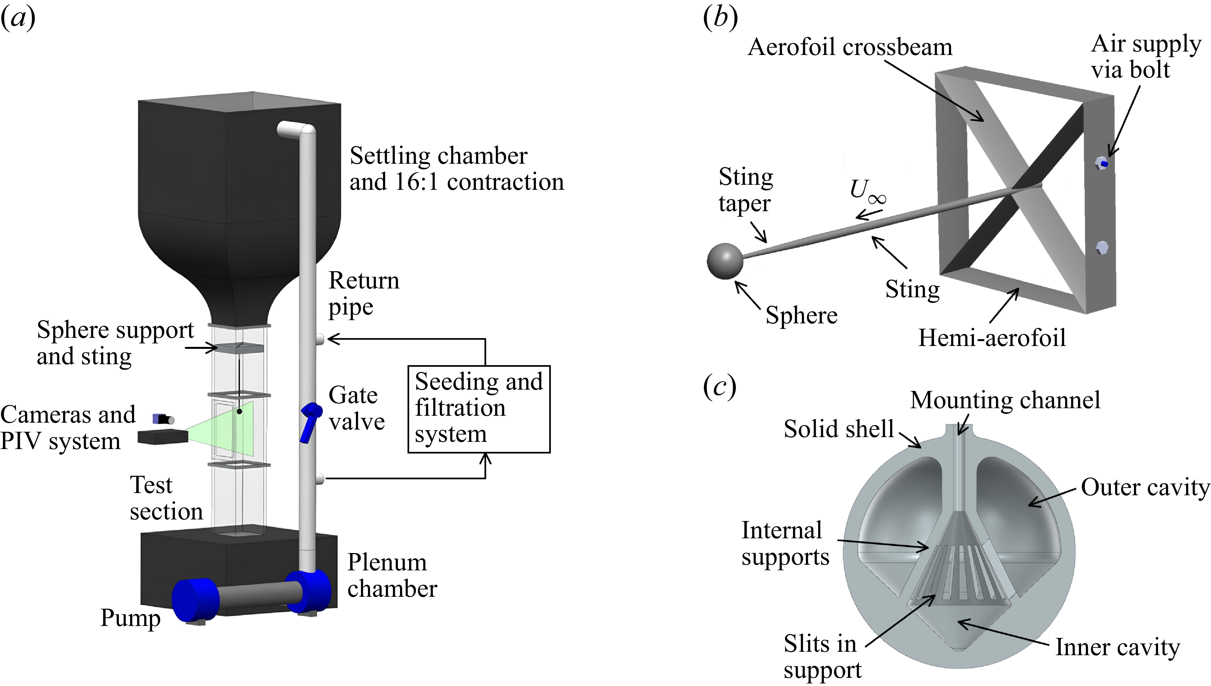
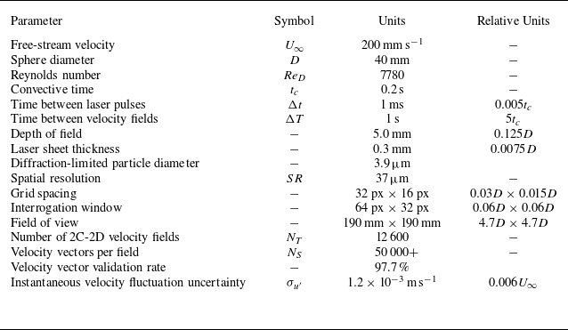
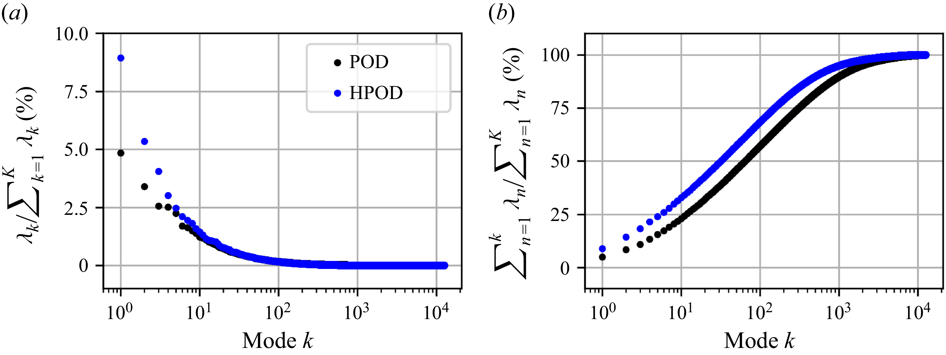
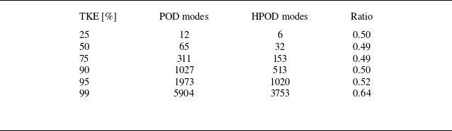


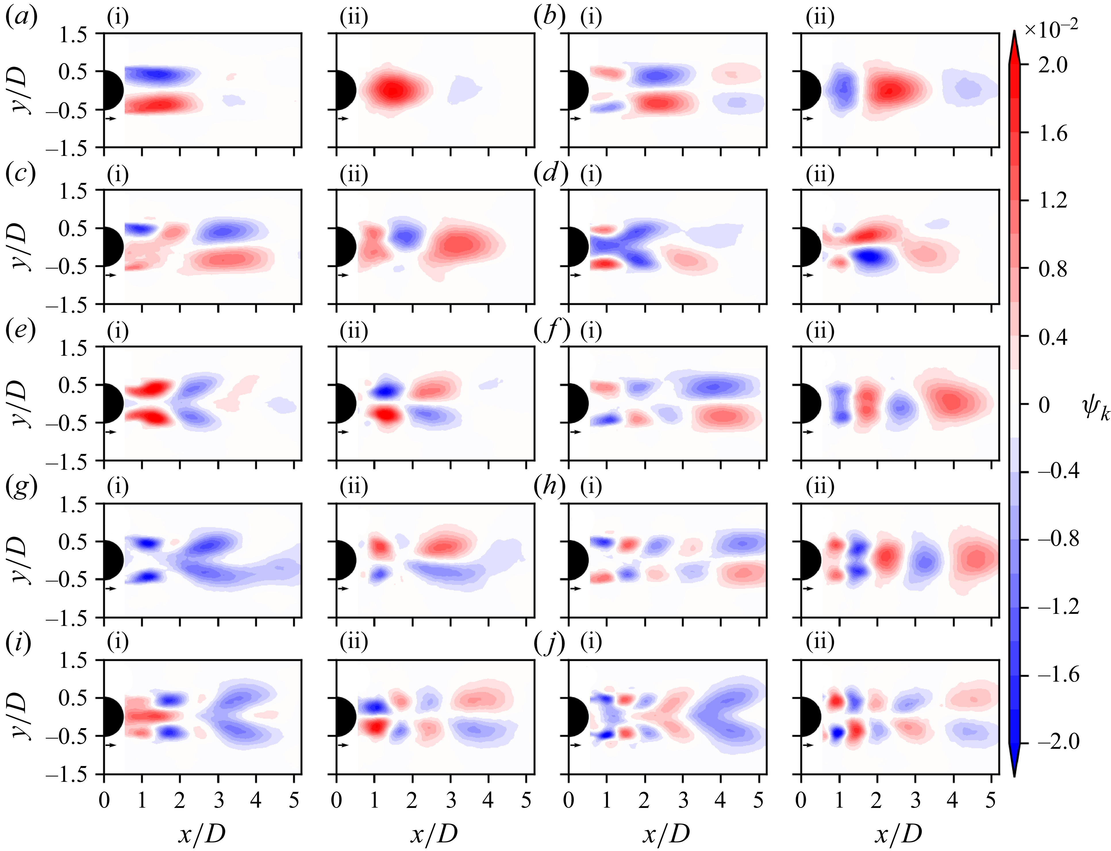
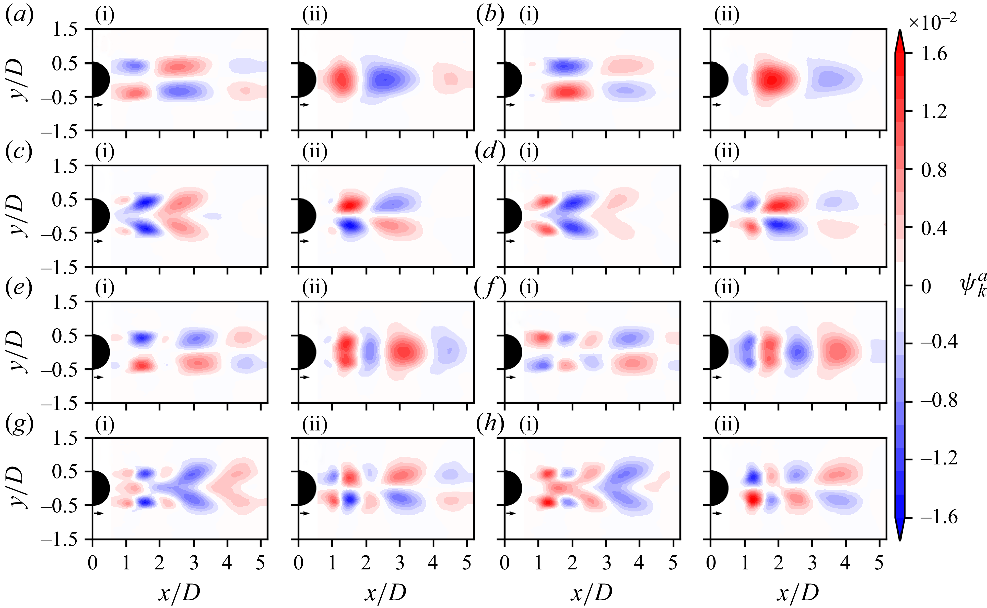
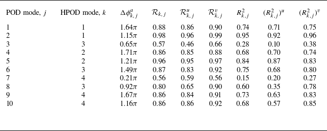


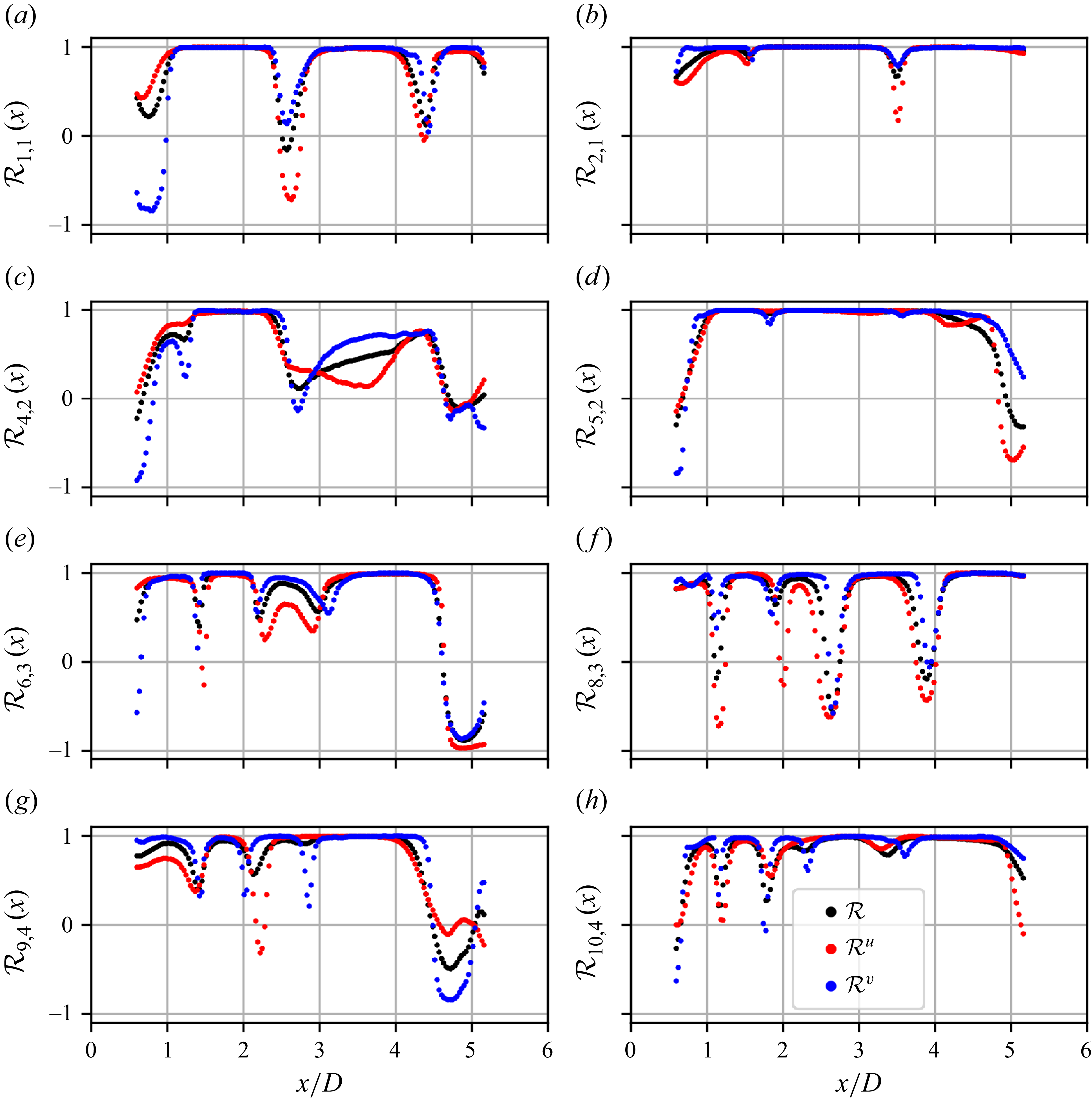


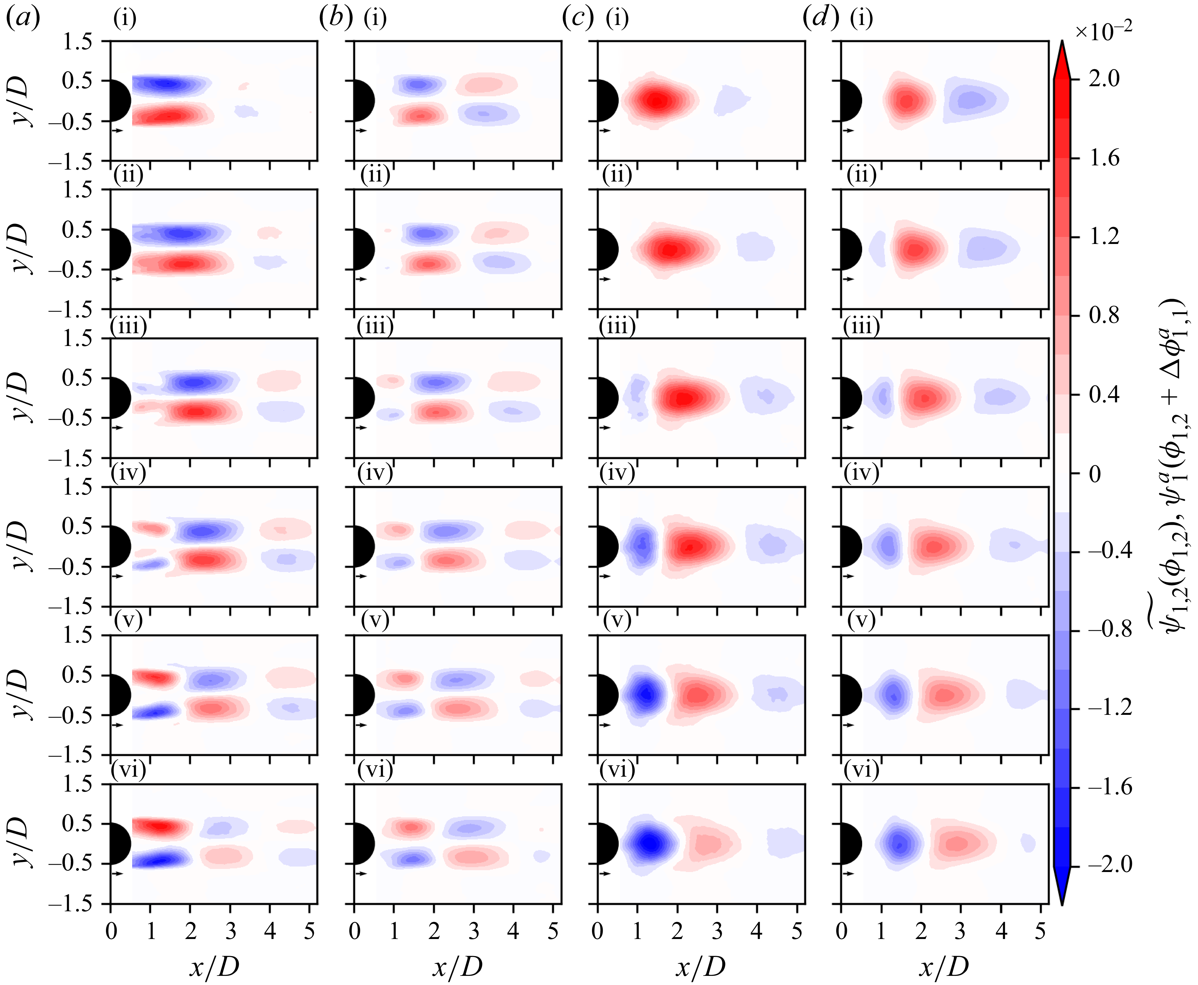


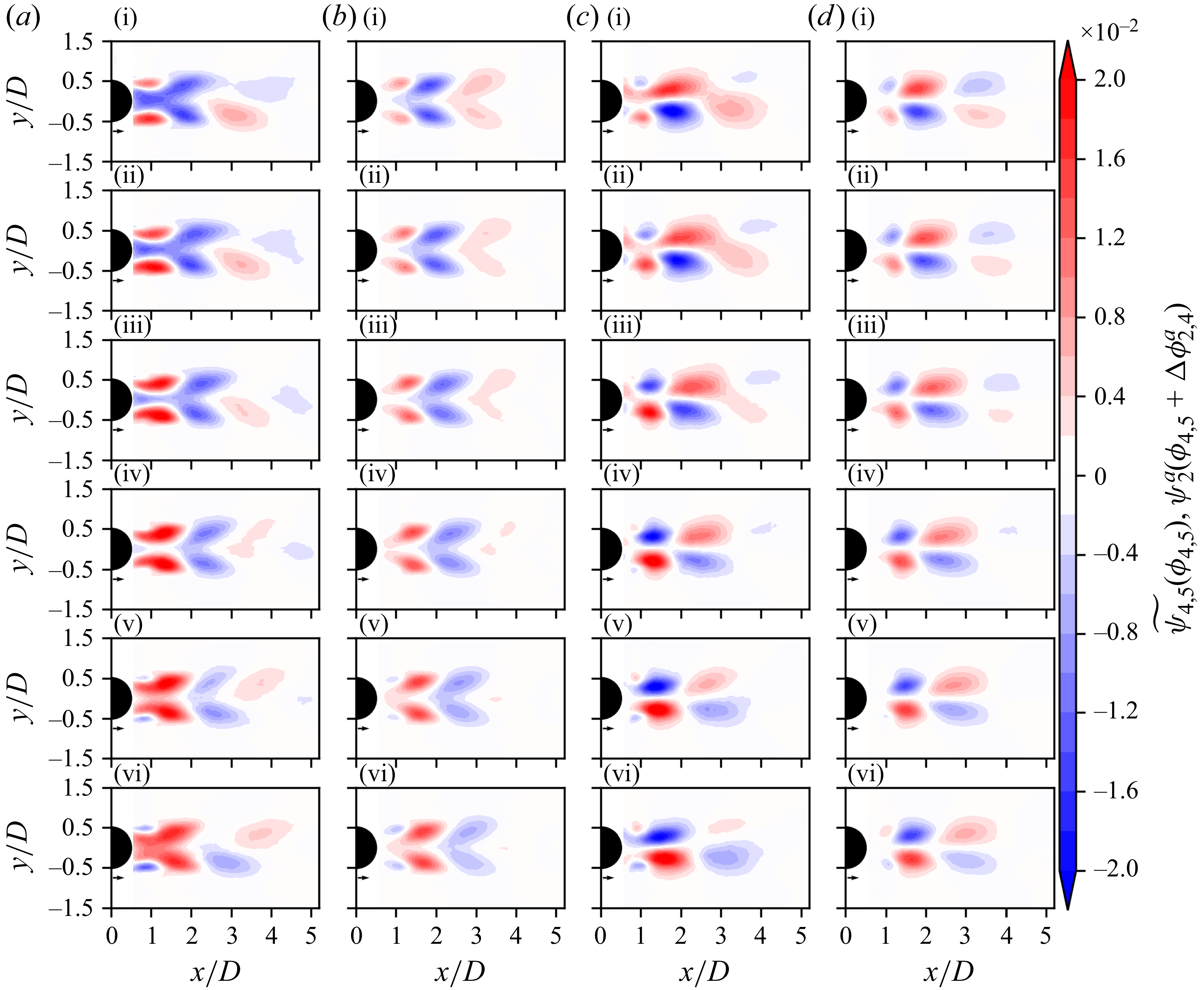


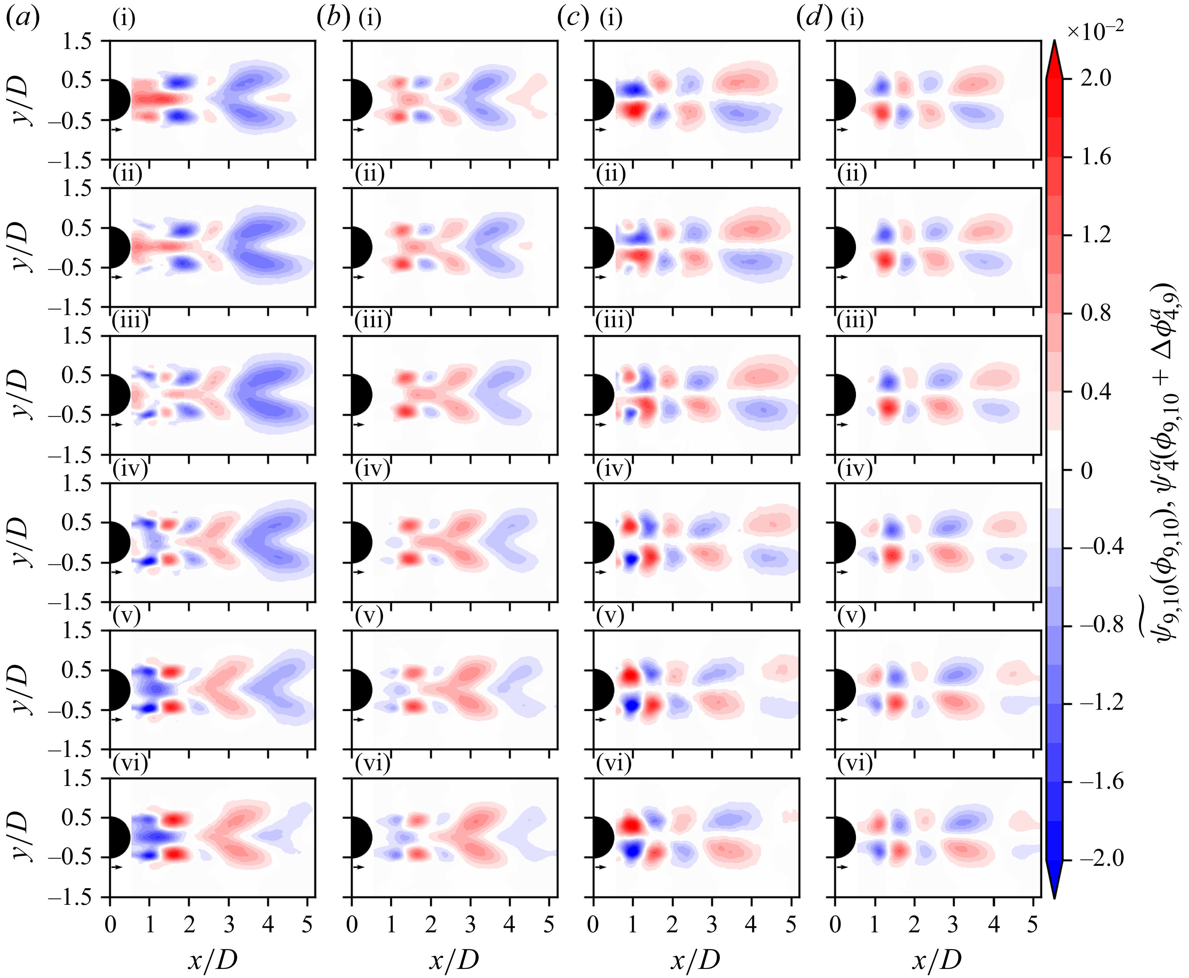


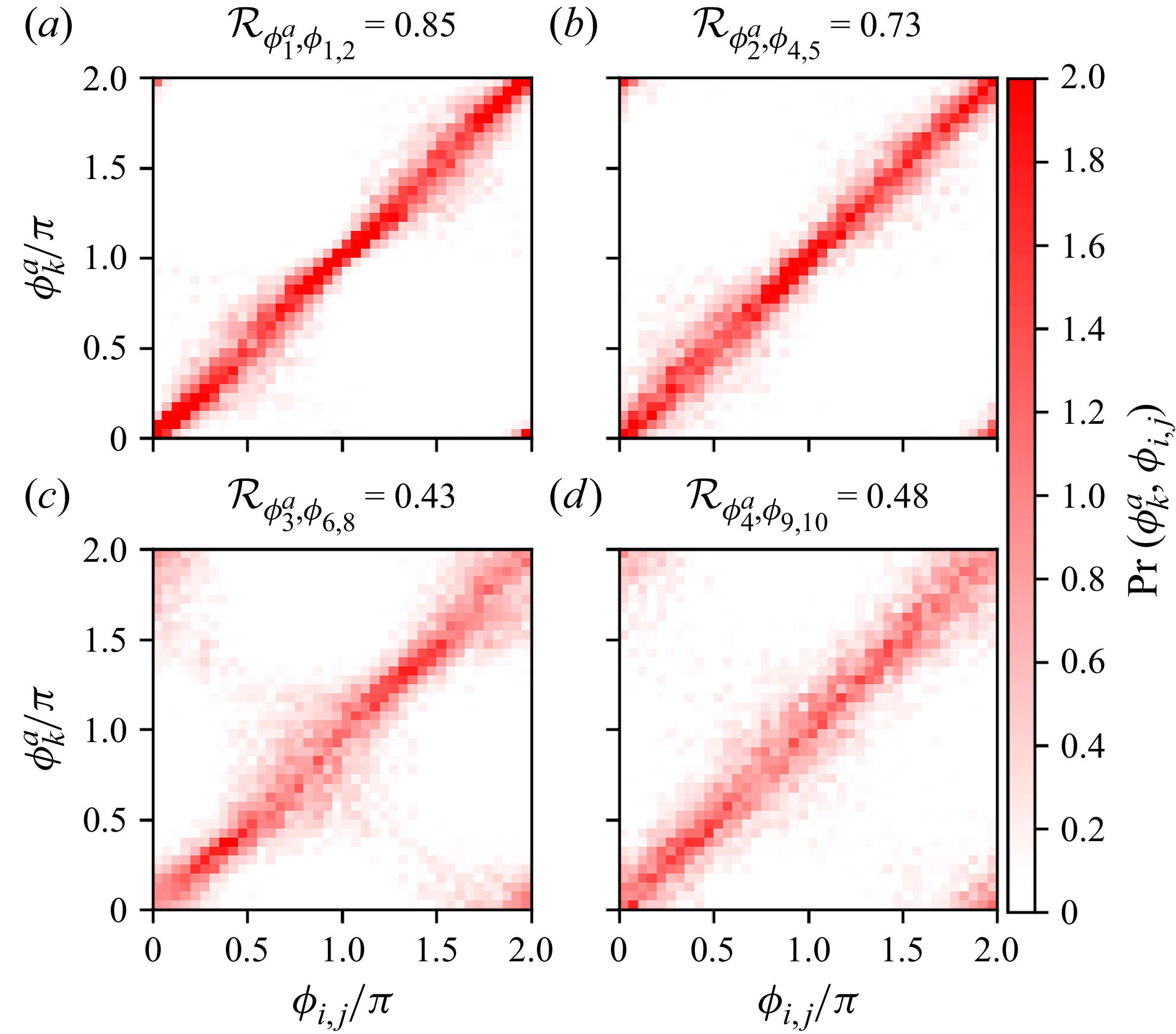
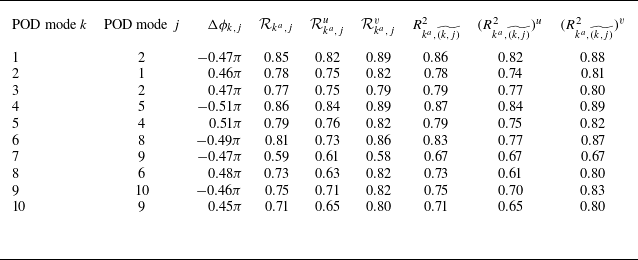


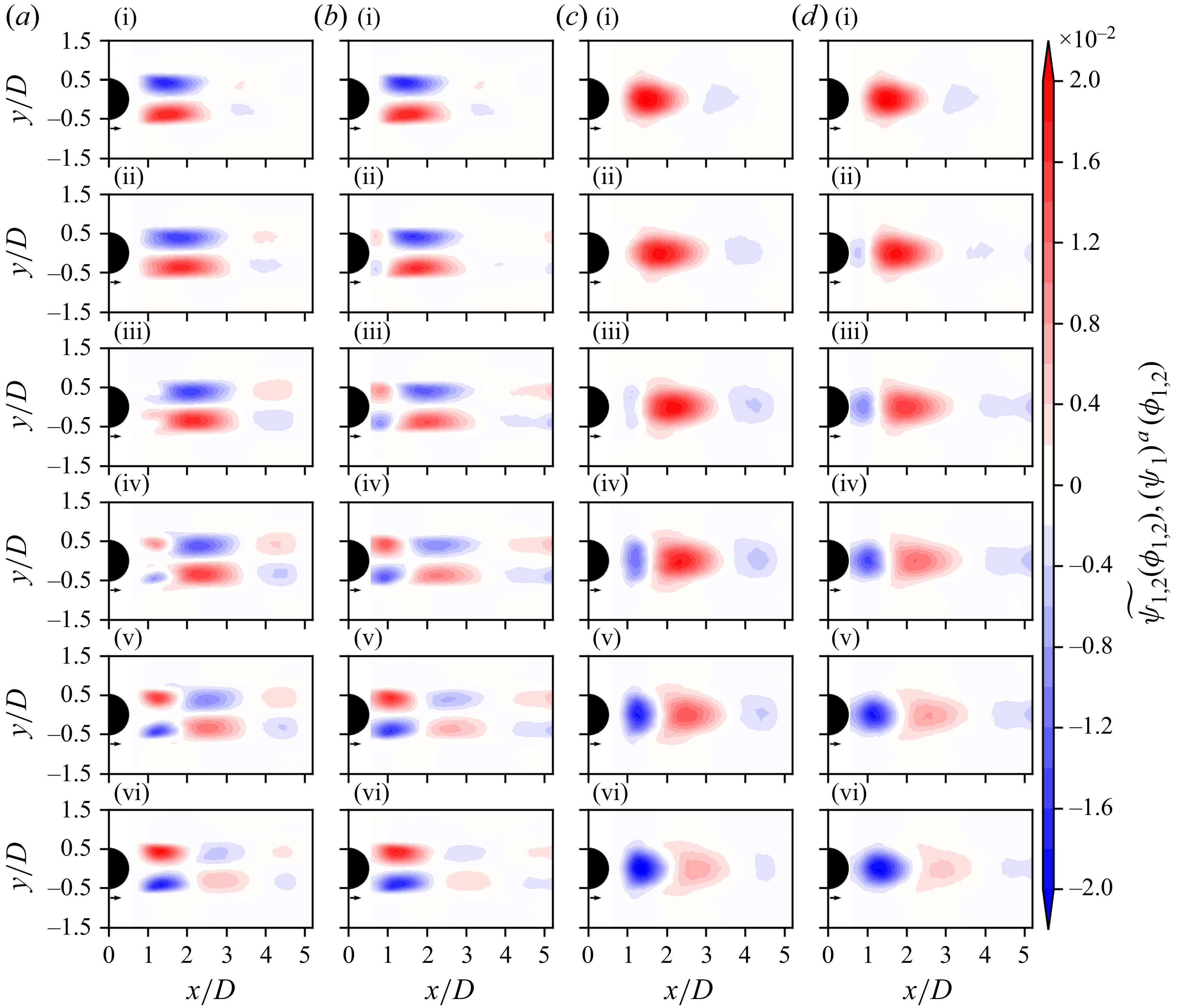


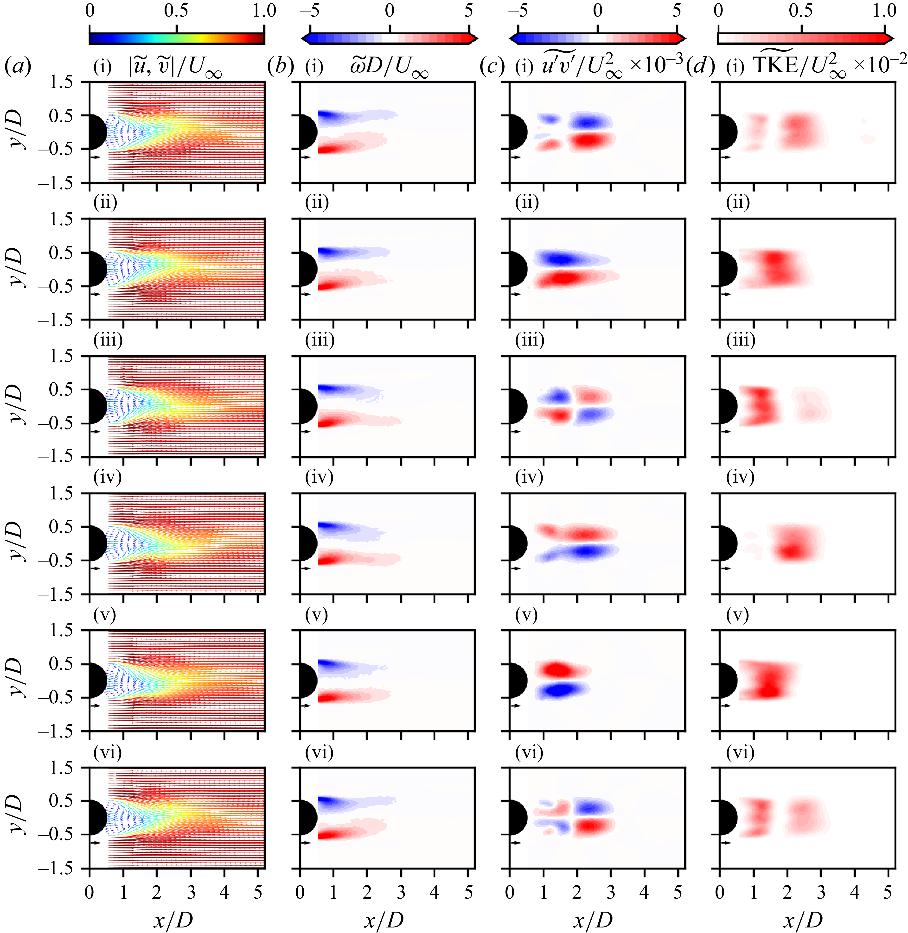


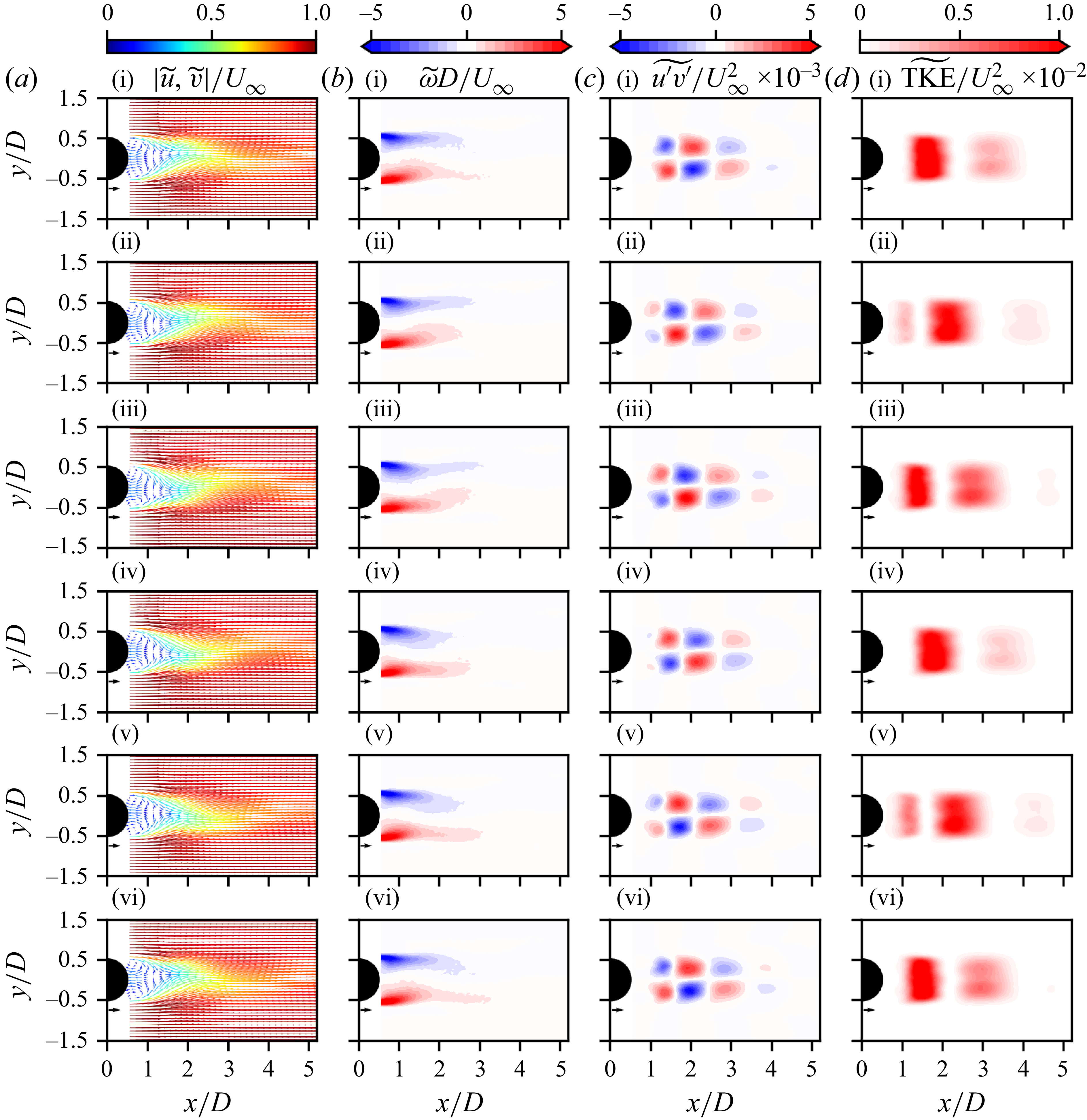


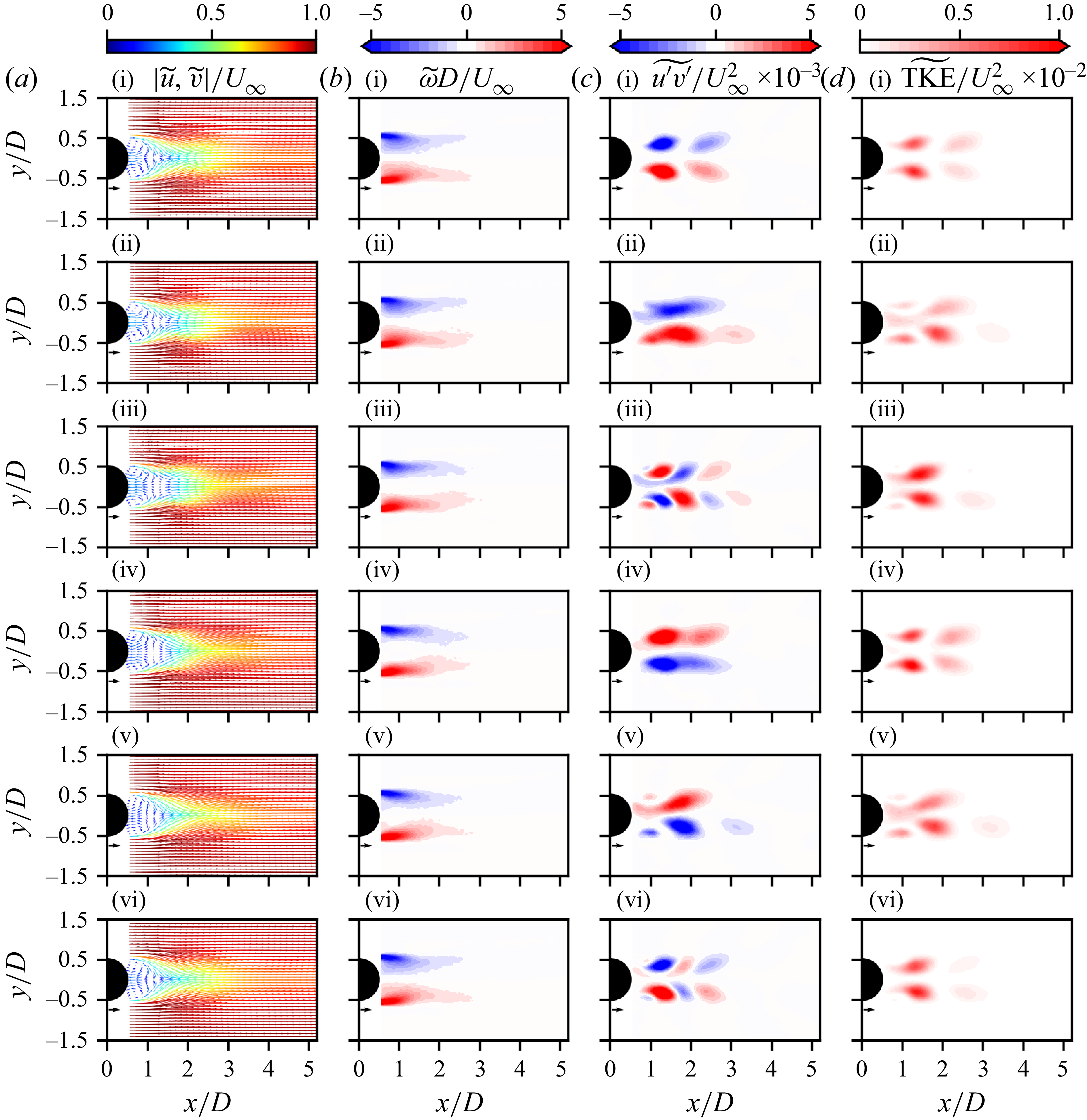


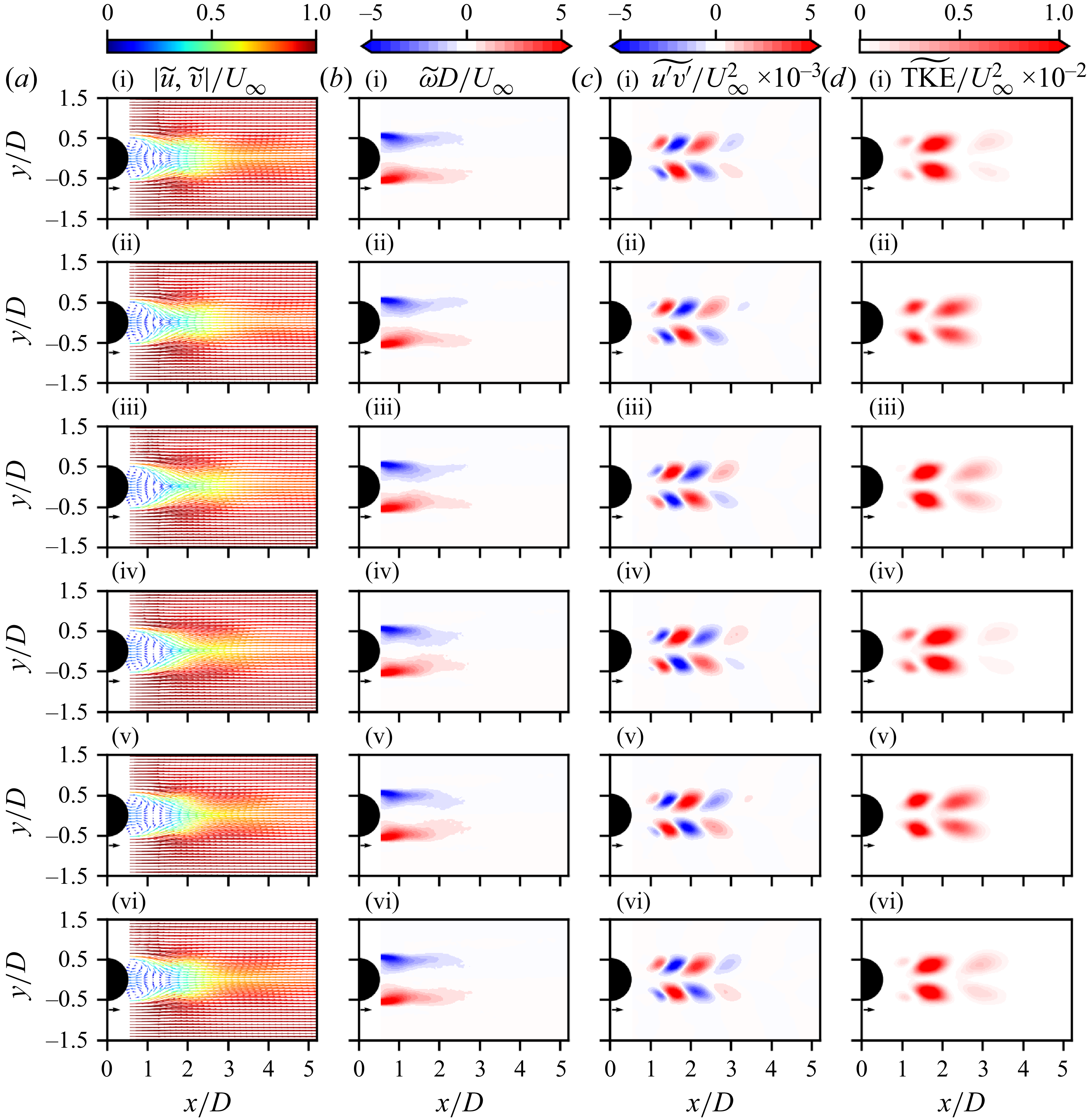


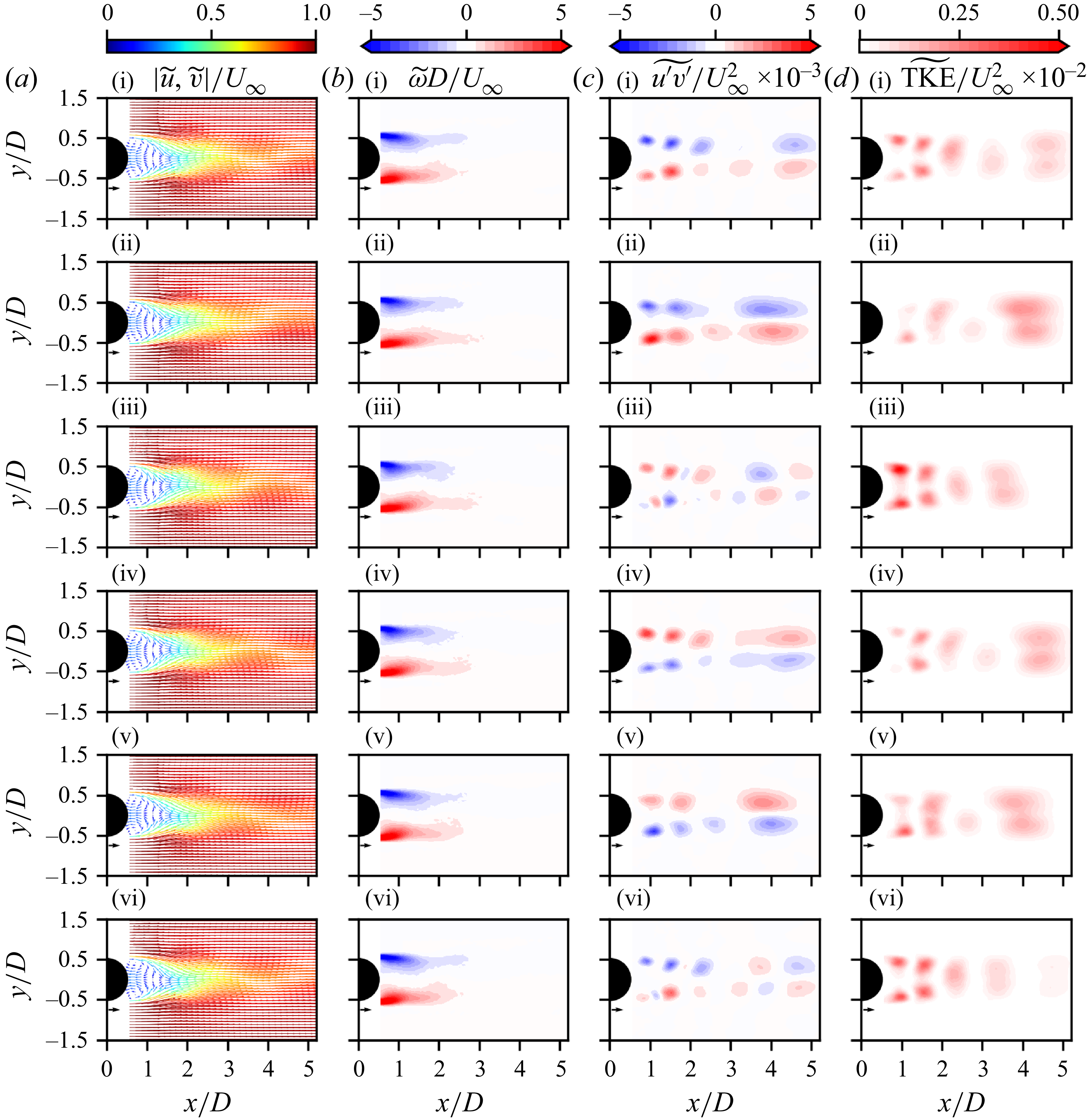


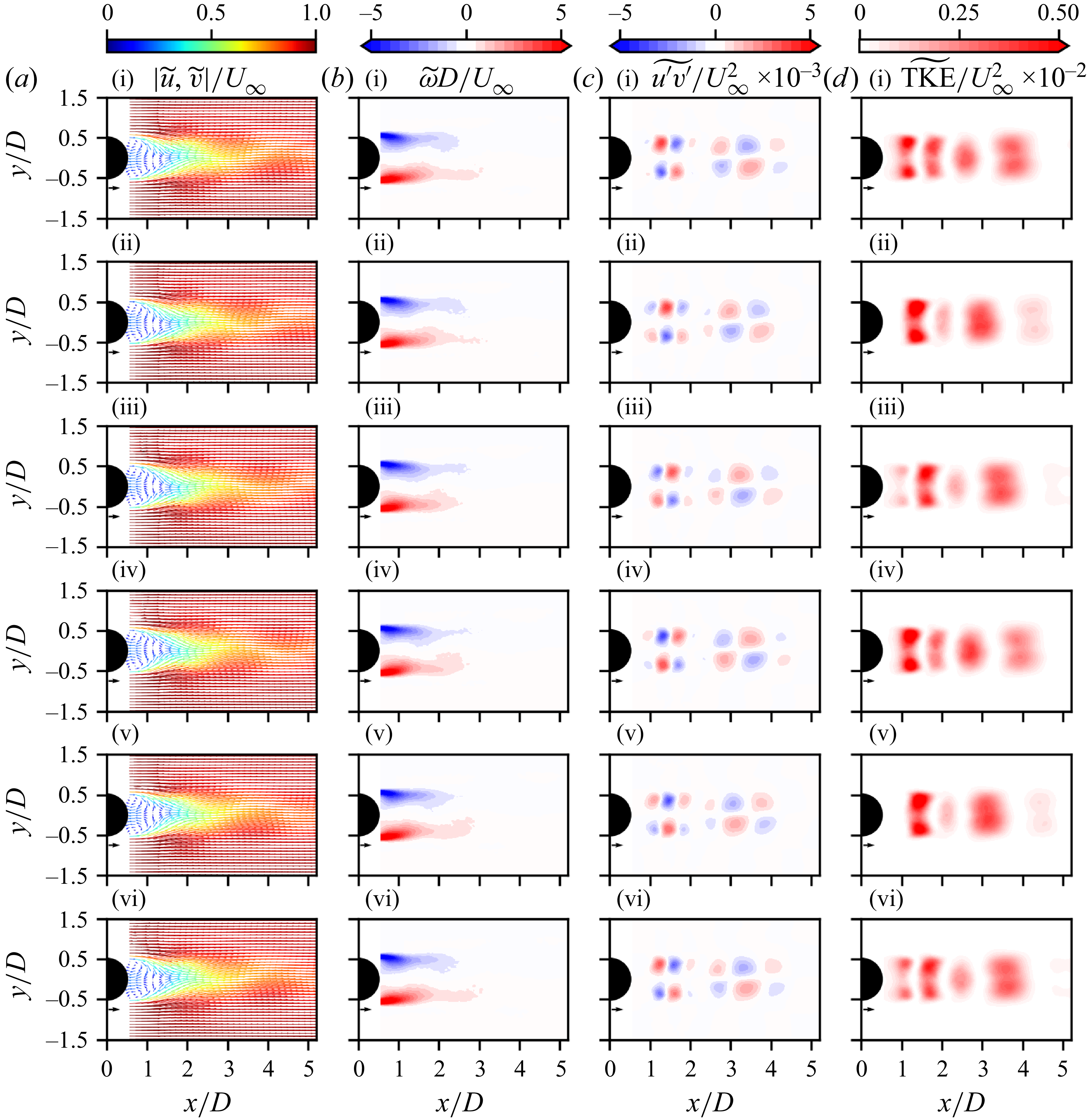


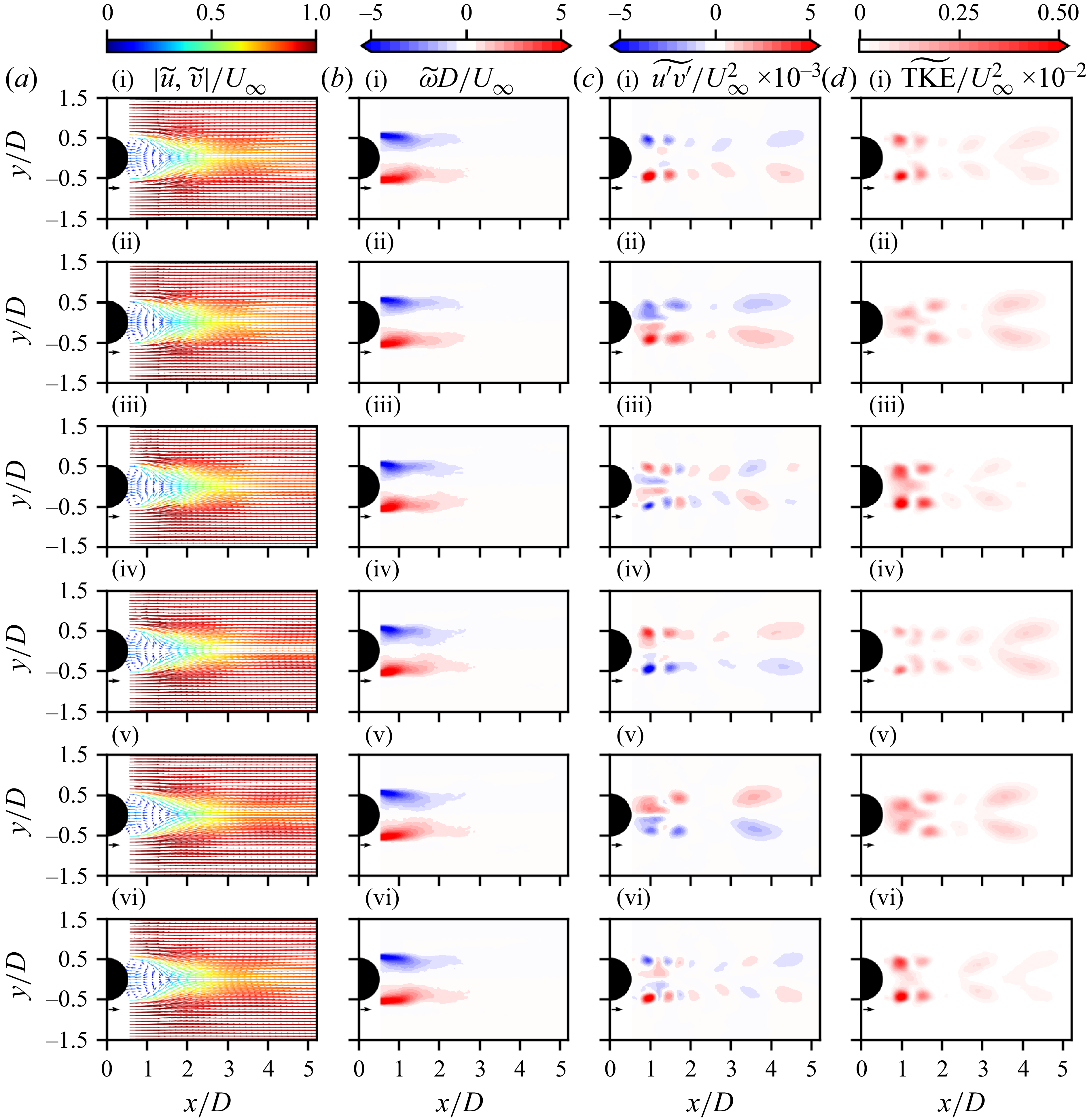


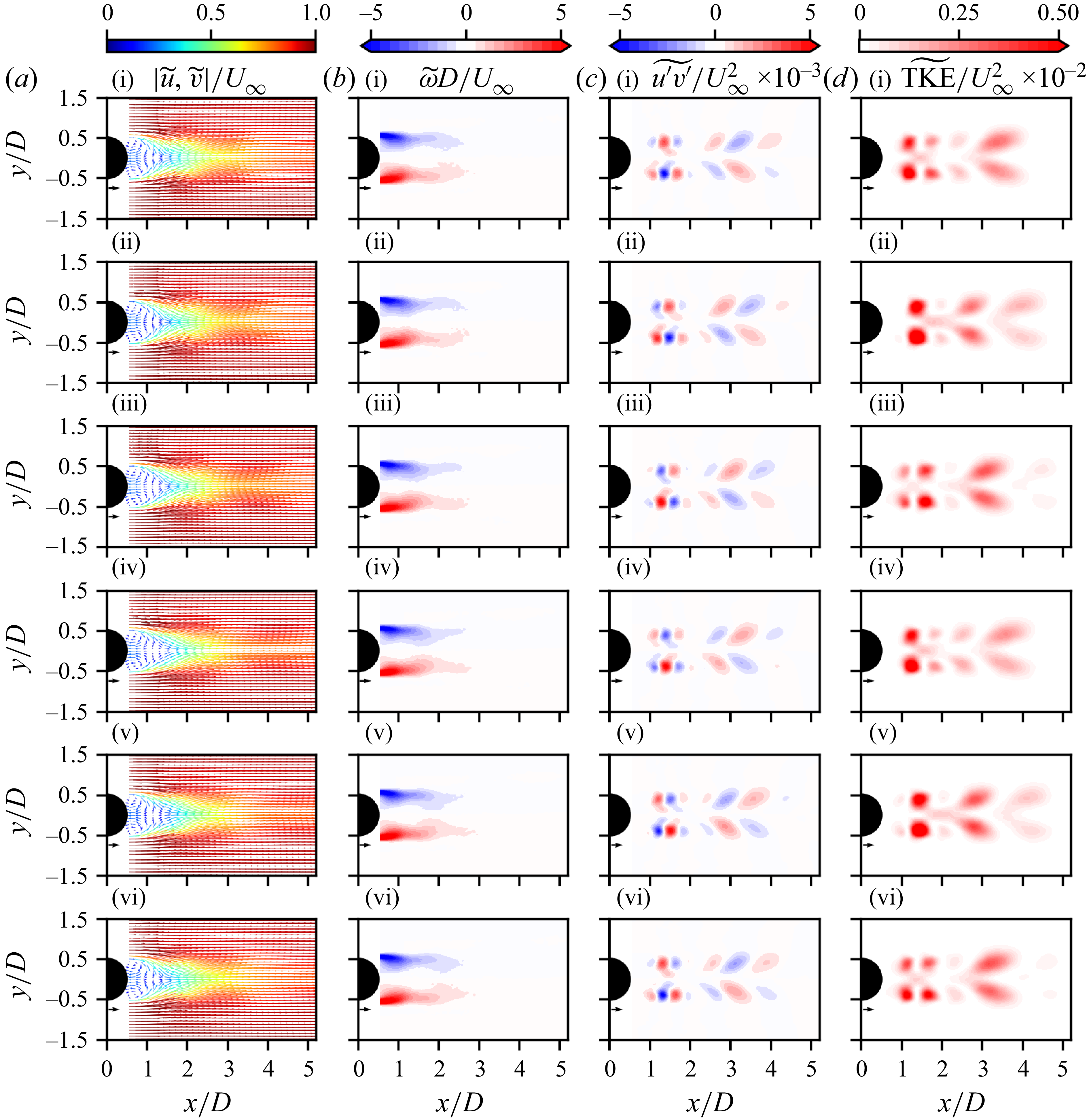


 Open access