


1. Introduction
Stellarators present a promising pathway to steady-state magnetic confinement fusion, offering inherent stability and low recirculating power requirements due to their reliance on externally generated magnetic fields. Unlike the axisymmetric design of tokamaks, stellarators are not constrained by continuous geometric symmetry. This freedom enables the engineering of complex, fully three-dimensional magnetic fields, broadening the range of possible configurations and allowing precise tailoring of magnetic geometry to enhance performance. While this geometric flexibility is a central advantage, it also renders confinement highly sensitive to shape; without deliberate and careful design, stellarators are susceptible to increased orbit losses and degraded transport. As a result, boundary-shape optimisation plays a critical role in realising the potential benefits of stellarator-based fusion devices.
(a) QA and (b) QH optimisation objective history comparison and final 3-D stellarator configuration. The red line shows the objective history with full spectrum using Moré Jacobian scaling as described in Appendix B, the green line shows the objective history with Fourier continuation using Moré Jacobian scaling and the gold line shows the objective history with full spectrum using ESS.

Stellarator optimisation traditionally separates the problem into (i) optimising the plasma boundary shape (Nührenberg & Zille Reference Nührenberg and Zille1988; Grieger et al. Reference Grieger1992; Mynick Reference Mynick2006; Bader et al. Reference Bader, Drevlak, Anderson, Faber, Hegna, Likin, Schmitt and Talmadge2019; Landreman & Paul Reference Landreman and Paul2022) and (ii) designing coils that reproduce that boundary shape (Merkel Reference Merkel1987; Drevlak Reference Drevlak1998; Boozer Reference Boozer2000; Pomphrey et al. Reference Pomphrey2001; Zhu et al. Reference Zhu, Hudson, Song and Wan2018). We focus exclusively on the first stage. For the first stage, the conventional approach often includes Fourier continuation (Landreman et al. Reference Landreman, Medasani and Zhu2021b ), where low-order Fourier modes are optimised first before gradually introducing higher ones. While this staged approach aids convergence, it is computationally inefficient, often over-optimises low modes and depends on arbitrary hyperparameters that can create artificial convergence plateaus, as shown by the green objective history from figure 1. In contrast, the full-spectrum approach refers to optimising all Fourier modes simultaneously from the outset, without any staged mode introduction. Despite its conceptual simplicity, the full-spectrum approach is rarely adopted in practice because the high-dimensional parameter space can lead to slow convergence, poor optimisation performance and an increased likelihood of getting trapped in local minima, as shown by the red objective history in figure 1.
In this paper, we introduce exponential spectral scaling (ESS) as a direct method to address the mode amplitude disparity (MAD). ESS applies a mode-specific exponential scaling that significantly reduces MAD and improves the overall optimisation landscape. We evaluate ESS with different norm choices ( $L_1$
,
$L_1$
, $L_2$
and
$L_2$
and $L_{\infty }$
), demonstrating robust convergence across various stellarator configurations. While this work focuses exclusively on local optimisation, we expect ESS to be broadly compatible with global optimisation frameworks and may improve their efficiency as well. In particular, because any global optimisation algorithm requires box constraints, ESS also informs how to choose meaningful bounds in spectral space. As shown by the gold objective history line in figure 1 (which will be described in more detail in § 4.2), ESS consistently delivers faster and more reliable convergence within a general trust-region framework, while avoiding non-physical outcomes such as self-intersecting surfaces.
$L_{\infty }$
), demonstrating robust convergence across various stellarator configurations. While this work focuses exclusively on local optimisation, we expect ESS to be broadly compatible with global optimisation frameworks and may improve their efficiency as well. In particular, because any global optimisation algorithm requires box constraints, ESS also informs how to choose meaningful bounds in spectral space. As shown by the gold objective history line in figure 1 (which will be described in more detail in § 4.2), ESS consistently delivers faster and more reliable convergence within a general trust-region framework, while avoiding non-physical outcomes such as self-intersecting surfaces.
In various optimisation settings, imbalances between low- and high-spectral content – formalised here as MAD – have been previously noted. In stellarator research, Fourier continuation (Landreman et al. Reference Landreman, Medasani and Zhu2021b ) is typically used to mitigate such imbalance; penalisation of high-mode-number amplitudes has also been used (Singh et al. Reference Singh, Kruger, Bader, Zhu, Hudson and Anderson2020). In aerospace inverse design, gradient-limiting Sobolev filters or staged Fourier optimisation is used to dampen high-order shape perturbations and stabilise convergence (Masters et al. Reference Masters, Taylor, Rendall and Allen2017; Kedward, Allen & Rendall Reference Kedward, Allen and Rendall2020). Geophysical full-waveform inversion confronts analogous ‘cycle-skipping’ local minima by introducing multiscale frequency sweeps and convex misfit functions (Bunks et al. Reference Bunks, Saleck, Zaleski and Chavent1995; Sirgue & Pratt Reference Sirgue and Pratt2004; Pladys et al. Reference Pladys, Brossier, Li and Métivier2021). Within machine learning, spectral bias and F-principle reveal that networks learn low-frequency components first, inspiring frequency-aware objective functions and rescaling schemes (Rahaman et al. Reference Rahaman, Baratin, Arpit, Draxler, Lin, Hamprecht, Bengio and Courville2019; Xu et al. Reference Xu, Zhang, Luo, Xiao and Ma2019; Wang & Lai Reference Wang and Lai2024). These convergent insights across disciplines motivate our ESS as a principled physics-agnostic remedy for MAD.
2. Towards reducing the mode amplitude disparity
2.1. Spectral representation of the plasma boundary
Stellarator boundary shapes are typically represented using truncated double Fourier series in cylindrical coordinates. Most stellarator optimisation to date has used the VMEC representation, in which $ R$
and
$ R$
and $ Z$
are expanded as cosine and sine series in the form
$ Z$
are expanded as cosine and sine series in the form $ \cos (m\theta - n N_{\mathrm{FP}}\phi )$
. In this paper, we instead adopt the related but distinct DESC representation defined by
$ \cos (m\theta - n N_{\mathrm{FP}}\phi )$
. In this paper, we instead adopt the related but distinct DESC representation defined by
 \begin{align} R(\theta ,\zeta ) &= \sum _{m=-M}^{M}\sum _{n=-N}^{N} R_n^m \, \mathcal{G}_n^m(\theta ,\zeta ), \end{align}
 \begin{align} Z(\theta ,\zeta ) &= \sum _{m=-M}^{M}\sum _{n=-N}^{N} Z_n^m \, \mathcal{G}_n^m(\theta ,\zeta ), \end{align}
where $\theta \in [0,2\pi )$
, the normalised toroidal angle is defined as
$\theta \in [0,2\pi )$
, the normalised toroidal angle is defined as $\zeta =\phi /N_{\mathrm{FP}}\in [0,2\pi )$
and the basis functions
$\zeta =\phi /N_{\mathrm{FP}}\in [0,2\pi )$
and the basis functions $\mathcal{G}_n^m(\theta ,\zeta )$
are defined piecewise according to the signs of
$\mathcal{G}_n^m(\theta ,\zeta )$
are defined piecewise according to the signs of $m$
and
$m$
and $n$
:
$n$
:
 \begin{align} \mathcal{G}_n^m(\theta ,\zeta )= \begin{cases} \cos (|m|\theta )\cos (|n|\zeta ), & m,n\geqslant 0,\\ \cos (|m|\theta )\sin (|n|\zeta ), & m\geqslant 0,n\lt 0,\\ \sin (|m|\theta )\cos (|n|\zeta ), & m\lt 0,n\geqslant 0,\\ \sin (|m|\theta )\sin (|n|\zeta ), & m,n\lt 0. \end{cases} \end{align}
However, this representation leads to a wide variation in the magnitude of Fourier coefficients. This effect, which we refer to as mode amplitude disparity (MAD), has significant consequences for optimisation.
2.2. Numerical challenges from mode amplitude disparity
MAD refers to the dynamic range among the Fourier coefficients used to represent stellarator boundaries. To quantify this imbalance, we define the MAD as
 \begin{align} \mathrm{MAD} = \frac {\max _{(m,n)} |A_n^m|}{\min _{(m,n) \,:\, A_n^m \neq 0} |A_n^m|}, \end{align}
where $A_n^m$
is either
$A_n^m$
is either $R^m_n$
or
$R^m_n$
or $Z^m_n$
from (2.1) to (2.2). This metric captures the effective dynamic range across all modes, excluding identically vanishing coefficients, and highlights the challenges posed by extreme scale separation in spectral representations. This imbalance poses serious numerical challenges because optimisation algorithms are sensitive to the scale of variables. When parameters differ significantly in magnitude, the resulting subproblems are poorly conditioned, leading to instability, slow convergence or convergence to suboptimal minima (Nocedal & Wright Reference Nocedal and Wright2006, Sect. 2.2, p. 26). As shown in figure 2(a), the Fourier mode amplitudes for a typical configuration exhibit near-exponential decay, which is typical of spectral representations (see Appendix A for more details). These issues motivate the need for strategies that reduce the amplitude disparity while preserving geometric fidelity.
$Z^m_n$
from (2.1) to (2.2). This metric captures the effective dynamic range across all modes, excluding identically vanishing coefficients, and highlights the challenges posed by extreme scale separation in spectral representations. This imbalance poses serious numerical challenges because optimisation algorithms are sensitive to the scale of variables. When parameters differ significantly in magnitude, the resulting subproblems are poorly conditioned, leading to instability, slow convergence or convergence to suboptimal minima (Nocedal & Wright Reference Nocedal and Wright2006, Sect. 2.2, p. 26). As shown in figure 2(a), the Fourier mode amplitudes for a typical configuration exhibit near-exponential decay, which is typical of spectral representations (see Appendix A for more details). These issues motivate the need for strategies that reduce the amplitude disparity while preserving geometric fidelity.
(a) Mode amplitudes showing exponential decay for the Landreman–Paul QA stellarator (Landreman & Paul Reference Landreman and Paul2022). (b) Distribution of mode amplitudes before and after ESS.

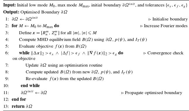
2.3. Fourier continuation as a mitigation strategy
Stellarator boundary optimisation seeks to minimise an objective function $ f(\boldsymbol{x})$
that quantifies how far a magnetic configuration deviates from desired physical properties. Given an initial boundary shape
$ f(\boldsymbol{x})$
that quantifies how far a magnetic configuration deviates from desired physical properties. Given an initial boundary shape $ \partial \varOmega ^{\text{init}}$
, a pressure profile
$ \partial \varOmega ^{\text{init}}$
, a pressure profile $ p(\psi )$
and a toroidal current profile
$ p(\psi )$
and a toroidal current profile $ I_T(\psi )$
, the optimisation iteratively adjusts Fourier coefficients
$ I_T(\psi )$
, the optimisation iteratively adjusts Fourier coefficients $ \boldsymbol{x} = [R_n^m, Z_n^m]$
until convergence. One conventional strategy for addressing the mode amplitude disparity (MAD) in this process is Fourier continuation (FC) – a staged approach that incrementally increases the maximum Fourier mode number from an initial low value
$ \boldsymbol{x} = [R_n^m, Z_n^m]$
until convergence. One conventional strategy for addressing the mode amplitude disparity (MAD) in this process is Fourier continuation (FC) – a staged approach that incrementally increases the maximum Fourier mode number from an initial low value $ M_0$
to a target
$ M_0$
to a target $ M_{\text{max}}$
. At each stage, the current solution initialises the next, introducing additional higher-order modes progressively. This allows the optimiser to start with a truncated, stable spectral representation and gradually refine it, as detailed in Algorithm 1.
$ M_{\text{max}}$
. At each stage, the current solution initialises the next, introducing additional higher-order modes progressively. This allows the optimiser to start with a truncated, stable spectral representation and gradually refine it, as detailed in Algorithm 1.
The rationale behind this approach is twofold: (i) low-order modes tend to dominate the global structure of the plasma boundary and are easier to optimise first; and (ii) introducing high-order modes incrementally avoids overwhelming the optimiser with ill-conditioned variables from the outset. This mitigates numerical instabilities and helps avoid convergence to poor local minima in early iterations. Beyond these theoretical advantages, Fourier continuation has proven effective in practice, consistently improving optimisation robustness across a range of configurations.
Although widely used, Fourier continuation relies on heuristic choices that are not necessarily optimal. The typical approach adds modes incrementally by bounding $\|m\|$
and
$\|m\|$
and $\|n\|$
at each step, but this specific ordering is arbitrary and may not align with the most relevant directions in parameter space. Such rigid heuristics can slow convergence or bias solutions towards subspaces favoured by early mode choices.
$\|n\|$
at each step, but this specific ordering is arbitrary and may not align with the most relevant directions in parameter space. Such rigid heuristics can slow convergence or bias solutions towards subspaces favoured by early mode choices.
Stellarator boundary optimisation with Fourier continuation

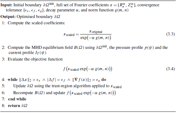
3. Exponential spectral scaling (ESS) methodology
Having outlined the challenges posed by mode amplitude disparities and the limitations of existing mitigation strategies, we now introduce exponential spectral scaling (ESS) – a principled method for rebalancing spectral coefficients prior to optimisation. This section presents the mathematical formulation of ESS, describes how it integrates into the optimisation workflow, and evaluates its effects on numerical performance and shape evolution. We begin by denoting the original Fourier coefficients representing the stellarator boundary as
 \begin{align} \boldsymbol{x}_{\text{original}} = [R_n^m,\, Z_n^m]. \end{align}
The ESS transformation is defined by
 \begin{align} \boldsymbol{x}_{\text{scaled}} = \frac {\boldsymbol{x}_{\text{original}}}{\exp \!\left (-\alpha \, g(m,n)\right )}, \end{align}
where $\alpha \geqslant 0$
is a user-specified decay parameter that controls the degree of scaling and
$\alpha \geqslant 0$
is a user-specified decay parameter that controls the degree of scaling and $g(m,n)$
is mode norm function that assigns relative importance to each spectral mode indexed by
$g(m,n)$
is mode norm function that assigns relative importance to each spectral mode indexed by $(m,n)$
. We consider the following choices for
$(m,n)$
. We consider the following choices for $g(m,n)$
:
$g(m,n)$
: $g(m,n) = |m|+|n|$
produces a diamond-shaped profile (the
$g(m,n) = |m|+|n|$
produces a diamond-shaped profile (the $L_1$
norm);
$L_1$
norm); $g(m,n) = \sqrt {m^2+n^2}$
gives a circular profile (the
$g(m,n) = \sqrt {m^2+n^2}$
gives a circular profile (the $L_2$
norm);
$L_2$
norm); $g(m,n) = \max \{|m|,|n|\}$
results in a square profile (the
$g(m,n) = \max \{|m|,|n|\}$
results in a square profile (the $L_{\infty }$
norm). Each of these choices defines a distinct decay geometry in Fourier space. The exponential scaling preferentially reduces the magnitude of high-order modes, thereby compressing the dynamic range of
$L_{\infty }$
norm). Each of these choices defines a distinct decay geometry in Fourier space. The exponential scaling preferentially reduces the magnitude of high-order modes, thereby compressing the dynamic range of $x_{\text{original}}$
from 6–7 orders of magnitude to approximately 2–3, as shown in figure 2. Although this does not necessarily improve the condition number of the Hessian, it reshapes the optimisation landscape by down-weighting high-order directions.
$x_{\text{original}}$
from 6–7 orders of magnitude to approximately 2–3, as shown in figure 2. Although this does not necessarily improve the condition number of the Hessian, it reshapes the optimisation landscape by down-weighting high-order directions.
To calibrate a practical decay rate, we analysed a library of stellarator configurations drawn from Kappel, Landreman & Malhotra (Reference Kappel, Landreman and Malhotra2024). Exponential decays of the form $\exp (-\alpha g(m,n))$
were fitted to the Fourier coefficients, using
$\exp (-\alpha g(m,n))$
were fitted to the Fourier coefficients, using $\log (|A^m_n|)$
in the regression and reporting
$\log (|A^m_n|)$
in the regression and reporting $R^2$
values to quantify fit quality; figure 2 shows one representative example. As shown in figure 3, for
$R^2$
values to quantify fit quality; figure 2 shows one representative example. As shown in figure 3, for $L_2$
and
$L_2$
and $L_\infty$
, the fitted decay rates
$L_\infty$
, the fitted decay rates $\alpha$
cluster between approximately 1.1 and 2.8, while for
$\alpha$
cluster between approximately 1.1 and 2.8, while for $L_1$
, the range is narrower and the fits are systematically worse. A likely reason is that stage-1 optimisations with Fourier continuation are typically based on square domains in
$L_1$
, the range is narrower and the fits are systematically worse. A likely reason is that stage-1 optimisations with Fourier continuation are typically based on square domains in $(m,n)$
space, which are more naturally aligned with
$(m,n)$
space, which are more naturally aligned with $L_\infty$
or
$L_\infty$
or $L_2$
geometries than with
$L_2$
geometries than with $L_1$
. The main takeaway from this survey is that reasonable choices of
$L_1$
. The main takeaway from this survey is that reasonable choices of $\alpha$
fall in the range
$\alpha$
fall in the range ${\sim} 1$
–3, providing both intuition for setting default values and justification for using
${\sim} 1$
–3, providing both intuition for setting default values and justification for using $L_\infty$
as the norm in subsequent experiments.
$L_\infty$
as the norm in subsequent experiments.
Conceptually, ESS is a fixed diagonal change of variables in coefficient space, chosen a priori from the expected spectral decay of physically meaningful equilibria. This stands in contrast to Newton and quasi-Newton methods, which build a local linear transformation from Hessian or inverse-Hessian information at the current iterate. In our highly nonlinear, non-convex stage-1 problem, this global rescaling remains stable even when local curvature information is unreliable or points towards directions that rapidly drive the magnetohydrodynamics (MHD) solver out of its convergence region.
Fitted decay rate $\alpha$
versus coefficient of determination
$\alpha$
versus coefficient of determination $R^2$
across a survey of stellarators. For
$R^2$
across a survey of stellarators. For $L_2$
and
$L_2$
and $L_\infty$
decay geometries,
$L_\infty$
decay geometries, $\alpha$
typically falls in the range
$\alpha$
typically falls in the range $1.1\!-\!2.8$
; for
$1.1\!-\!2.8$
; for $L_1$
, the range is narrower (
$L_1$
, the range is narrower ( $0.7 \leqslant \alpha \leqslant 1.9$
) and fit quality is generally lower (
$0.7 \leqslant \alpha \leqslant 1.9$
) and fit quality is generally lower ( $-0.3 \leqslant R^2 \leqslant 0.77$
).
$-0.3 \leqslant R^2 \leqslant 0.77$
).

Building on the above-mentioned formulation, ESS is applied as a mode-dependent variable rescaling of the Fourier coefficient vector $x_{\text{original}}$
prior to optimisation. Once scaled, the optimisation proceeds over
$x_{\text{original}}$
prior to optimisation. Once scaled, the optimisation proceeds over $x_{\text{scaled}}$
using a standard algorithm (e.g. trust-region method). In practice, ESS can be conveniently implemented by setting the x_scale keyword argument in scipy.optimise.least_squares. Algorithm 2 outlines the ESS-based optimisation procedure without the loop over
$x_{\text{scaled}}$
using a standard algorithm (e.g. trust-region method). In practice, ESS can be conveniently implemented by setting the x_scale keyword argument in scipy.optimise.least_squares. Algorithm 2 outlines the ESS-based optimisation procedure without the loop over $M$
from Algorithm 1.
$M$
from Algorithm 1.
Stellarator boundary optimisation with ESS

As a result, the optimiser is able to take more meaningful steps early in the optimisation process, without becoming trapped in ill-conditioned subspaces. We hypothesise that the balanced scaling results in a smoother and more navigable optimisation landscape, effectively serving as a continuous analogue to Fourier continuation. By enabling direct full-spectrum optimisation, ESS obviates the need for arbitrary staging decisions and the staged mode activation required by traditional Fourier continuation methods. This reduces computational overhead and allows the optimiser to operate in a rescaled coefficient space that better reflects the underlying spectral structure.
High-order Fourier modes are often associated with fine-scale features on the plasma boundary that are difficult to resolve numerically and may not correspond to physically meaningful structures. If left unconstrained, these modes can introduce artificial oscillations, kinks or even self-intersections in the boundary geometry. ESS reduces the influence of these high-order components early in the optimisation process by attenuating their amplitudes. This prioritises smooth, well-resolved shape components. Importantly, ESS does not remove high-order modes; it simply ensures that their effect is proportionate to their representational significance. In § 4, we present empirical evidence showing that ESS results in a smoother and faster convergence without instances of pathological geometries.
4. Numerical experiment results
We evaluate the performance of ESS on two benchmark stellarator configurations: Landreman–Paul quasi-axisymmetric (QA) and quasi-helically symmetric (QH) confifigurations (Landreman & Paul Reference Landreman and Paul2022). Our experimental comparisons focus on convergence dynamics, computational efficiency and the quality of the resulting plasma boundary shapes.
4.1. Optimisation problem
The optimisation problem solved by Landreman & Paul (Reference Landreman and Paul2022) determines a stellarator boundary that minimises quasisymmetry errors while meeting the target rotational transform and aspect ratio goals. The independent variables are the Fourier coefficients of the plasma boundary represented in § 2, truncated to a maximum poloidal and toroidal mode number of $ m_{\max } = n_{\max } = 6$
. These independent variables collect into the vector
$ m_{\max } = n_{\max } = 6$
. These independent variables collect into the vector $\boldsymbol{x} = [R_n^m, Z_n^m]$
. The total objective is a weighted sum of three terms,
$\boldsymbol{x} = [R_n^m, Z_n^m]$
. The total objective is a weighted sum of three terms,
 \begin{align} f(\boldsymbol x)= w_{\mathrm{QS}}f_{\mathrm{QS}}+ w_{\bar \iota }f_{\bar \iota }+ w_{A}f_{A}, \end{align}
where $w_{\mathrm{QS}}$
,
$w_{\mathrm{QS}}$
, $w_{\bar \iota }$
and
$w_{\bar \iota }$
and $w_{A}$
are user-chosen positive weights, all chosen to be 1 in this study. Following Landreman & Paul (Reference Landreman and Paul2022), the error in quasisymmetry is measured by
$w_{A}$
are user-chosen positive weights, all chosen to be 1 in this study. Following Landreman & Paul (Reference Landreman and Paul2022), the error in quasisymmetry is measured by
 \begin{align} f_{\mathrm{QS}} = \int _V \biggl [ \frac {1}{B^{3}} ( (N - \iota M)\, \boldsymbol{B} \times \boldsymbol{\nabla }B \boldsymbol{\cdot }\boldsymbol{\nabla }\psi - (M G + N I)\, \boldsymbol{B} \boldsymbol{\cdot }\boldsymbol{\nabla }B ) \biggr ]^2 \, \mathrm{d}^3x, \end{align}
where the integral is taken over the plasma volume $V$
. Here,
$V$
. Here, $M$
and
$M$
and $N$
are the integers defining the desired symmetry type,
$N$
are the integers defining the desired symmetry type, $G(\psi )$
is
$G(\psi )$
is $\mu _0/(2\pi )$
times the poloidal current outside the surface and
$\mu _0/(2\pi )$
times the poloidal current outside the surface and $I(\psi )$
is
$I(\psi )$
is $\mu _0/(2\pi )$
times the toroidal current inside the surface. For all computations in this work,
$\mu _0/(2\pi )$
times the toroidal current inside the surface. For all computations in this work, $M = 1$
and
$M = 1$
and $I = 0$
, though we retain the general form of the equation for completeness. Instead of penalising the difference between the realised and target rotational transforms on every surface, we use a single mean
$I = 0$
, though we retain the general form of the equation for completeness. Instead of penalising the difference between the realised and target rotational transforms on every surface, we use a single mean $\bar {\iota } = \int _{0}^{1} {\rm d}s \,\iota \,$
, and define
$\bar {\iota } = \int _{0}^{1} {\rm d}s \,\iota \,$
, and define
 \begin{equation} f_{\bar \iota }= [\bar \iota -\bar \iota _{\mathrm{tar}}]^{2},\quad \bar {\iota }_{\mathrm{tar}} \; \text{is a specified target value}. \end{equation}
Lastly, the aspect ratio is $A=R/a$
, so that
$A=R/a$
, so that
 \begin{equation} f_{A}=[A(\boldsymbol x)-A_{\mathrm{tar}}]^{2}. \end{equation}
Throughout this work, we adopt the target values $(\iota _{\text{tar}},A_{\text{tar}})=(0.42,\,6.0)$
for the quasi-axisymmetric (QA,
$(\iota _{\text{tar}},A_{\text{tar}})=(0.42,\,6.0)$
for the quasi-axisymmetric (QA, $N_{\mathrm{FP}}=2$
) configuration and
$N_{\mathrm{FP}}=2$
) configuration and $(\iota _{\text{tar}},A_{\text{tar}})=(1.24,\,8.0)$
for the quasi-helically symmetric (QH,
$(\iota _{\text{tar}},A_{\text{tar}})=(1.24,\,8.0)$
for the quasi-helically symmetric (QH, $N_{\mathrm{FP}}=4$
) configuration. Except for figure 7 showing the efficacy of ESS in simsopt (Landreman et al. Reference Landreman, Medasani, Wechsung, Giuliani, Jorge and Zhu2021a
), optimisations were carried out with the desc code (Panici et al. Reference Panici, Conlin, Dudt, Unalmis and Kolemen2023). The optimisation was performed using the trust-region reflective (TRF) algorithm, as implemented in scipy.optimise.least_squares with method=’trf’. Comparable results were also obtained using the Levenberg–Marquardt (LM) algorithm from MINPACK. Initial conditions are based on rotating elliptical boundary shapes.
$N_{\mathrm{FP}}=4$
) configuration. Except for figure 7 showing the efficacy of ESS in simsopt (Landreman et al. Reference Landreman, Medasani, Wechsung, Giuliani, Jorge and Zhu2021a
), optimisations were carried out with the desc code (Panici et al. Reference Panici, Conlin, Dudt, Unalmis and Kolemen2023). The optimisation was performed using the trust-region reflective (TRF) algorithm, as implemented in scipy.optimise.least_squares with method=’trf’. Comparable results were also obtained using the Levenberg–Marquardt (LM) algorithm from MINPACK. Initial conditions are based on rotating elliptical boundary shapes.
4.2. Stellarator optimisation results
(a) Objective histories for three optimisation methods under varying initial elongations. (b) Cross-sections of initial shape varying elongation values. (c) The stalled optimisations highlight the limitations of Moré scaling alone, without Fourier continuation, leading to distorted shapes. (d) Final cross-sections from Fourier continuation show much less variation than in panel (c), with only minor residual differences. (e) ESS yields consistent final boundaries with minimal run-to-run variation.

Figure 1 presents the objective history during optimisation, where ESS demonstrates a smoother and more rapid decrease in the objective function compared with the conventional Fourier continuation method. The vertical green lines mark the iterations at which the number of Fourier modes is increased – that is, where the $M$
in Algorithm 1 is incremented – thus expanding the degrees of freedom in the optimisation problem. For both the full-spectrum and Fourier continuation methods, Jacobian-based variable scaling is used via the x_scale=’jac’ setting in scipy.optimise.least_squares, as described in Appendix B. When x_scale is instead set to 1, the performance of full-spectrum optimisation degrades significantly, while Fourier continuation performs similarly with or without Jacobian scaling. Figure 1 compares the final three-dimensional (3-D) configurations for the QA and QH benchmarks obtained using ESS against those from Fourier continuation. For this figure, we employed the
$M$
in Algorithm 1 is incremented – thus expanding the degrees of freedom in the optimisation problem. For both the full-spectrum and Fourier continuation methods, Jacobian-based variable scaling is used via the x_scale=’jac’ setting in scipy.optimise.least_squares, as described in Appendix B. When x_scale is instead set to 1, the performance of full-spectrum optimisation degrades significantly, while Fourier continuation performs similarly with or without Jacobian scaling. Figure 1 compares the final three-dimensional (3-D) configurations for the QA and QH benchmarks obtained using ESS against those from Fourier continuation. For this figure, we employed the $L_{\infty }$
norm on
$L_{\infty }$
norm on $(m,n)$
with
$(m,n)$
with $\alpha =1.6$
. The direct full-spectrum optimisation enabled by ESS removes the need for arbitrary staging decisions and avoids the artificial convergence plateaus typically observed with Fourier continuation. The improved convergence and quality of the optimised configurations underscore the efficacy of ESS in stellarator boundary optimisation.
$\alpha =1.6$
. The direct full-spectrum optimisation enabled by ESS removes the need for arbitrary staging decisions and avoids the artificial convergence plateaus typically observed with Fourier continuation. The improved convergence and quality of the optimised configurations underscore the efficacy of ESS in stellarator boundary optimisation.
Figure 4 further compares the convergence histories of ESS, FC, as well as optimising the full spectrum of modes with $|m|, |n| \leqslant 6$
without FC for the QA problem across an ensemble of initial conditions varying initial elongations. Figure 4(
a
) shows the objective value versus iteration count for all three methods, with ESS consistently achieving faster convergence. Panels (d)–(e) display the final cross-sections at
$|m|, |n| \leqslant 6$
without FC for the QA problem across an ensemble of initial conditions varying initial elongations. Figure 4(
a
) shows the objective value versus iteration count for all three methods, with ESS consistently achieving faster convergence. Panels (d)–(e) display the final cross-sections at $\phi = 0$
with Fourier continuation and ESS, demonstrating that ESS reaches more consistent optima with less variation than FC. Figure 4(
c
) further illustrates that both FC and ESS resolve the issues seen in the full-spectrum case, with ESS requiring fewer iterations while FC attains slightly lower objective values. Here, we employ the
$\phi = 0$
with Fourier continuation and ESS, demonstrating that ESS reaches more consistent optima with less variation than FC. Figure 4(
c
) further illustrates that both FC and ESS resolve the issues seen in the full-spectrum case, with ESS requiring fewer iterations while FC attains slightly lower objective values. Here, we employ the $L_\infty$
norm on
$L_\infty$
norm on $(m,n)$
with
$(m,n)$
with $\alpha = 1.6$
.
$\alpha = 1.6$
.
4.3. Robustness to norm choice and decay rate
We conducted a systematic analysis of the ESS method across different norm functions and decay parameters $\alpha$
for the QA problem. Figure 5 illustrates the convergence behaviour for three norm types –
$\alpha$
for the QA problem. Figure 5 illustrates the convergence behaviour for three norm types – $L_1$
,
$L_1$
, $L_2$
and
$L_2$
and $L_{\infty }$
– as well as a sweep over various
$L_{\infty }$
– as well as a sweep over various $\alpha$
values. While all three norm types and the tested
$\alpha$
values. While all three norm types and the tested $\alpha$
values eventually reach similarly low objective values, some parameter choices achieve convergence quicker.
$\alpha$
values eventually reach similarly low objective values, some parameter choices achieve convergence quicker.
Objective histories for different ESS norm types (a) for $\alpha = 1.8$
and (b) for varying
$\alpha = 1.8$
and (b) for varying $\alpha$
values under
$\alpha$
values under $L_\infty$
scaling, for the QA problem.
$L_\infty$
scaling, for the QA problem.

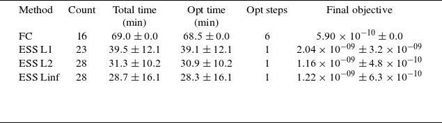
Figure 6 and table 1 further quantify robustness of ESS for the QA problem, showing the number of iterations required to reach a target objective of $10^{-8}$
for various
$10^{-8}$
for various $(\alpha , \text{norm})$
combinations. Robust convergence is observed for
$(\alpha , \text{norm})$
combinations. Robust convergence is observed for $\alpha$
values ranging from 0.5 to 3.3, with optimal performance typically occurring between 0.8 and 1.5. This performance-based window partially overlaps with the fitted decay rates reported in figure 3, which extend to higher values, especially for
$\alpha$
values ranging from 0.5 to 3.3, with optimal performance typically occurring between 0.8 and 1.5. This performance-based window partially overlaps with the fitted decay rates reported in figure 3, which extend to higher values, especially for $L_2$
and
$L_2$
and $L_\infty$
. The difference may arise because the fitted
$L_\infty$
. The difference may arise because the fitted $\alpha$
describes geometric decay in final equilibria, while the algorithmic
$\alpha$
describes geometric decay in final equilibria, while the algorithmic $\alpha$
governs progress along the optimisation path. The absence of a marker indicates that the objective was not reduced below
$\alpha$
governs progress along the optimisation path. The absence of a marker indicates that the objective was not reduced below $10^{-8}$
, which is rare in the tested range. All ESS variants demonstrate successful convergence across a wide range of hyperparameters. In particular, the
$10^{-8}$
, which is rare in the tested range. All ESS variants demonstrate successful convergence across a wide range of hyperparameters. In particular, the $L_2$
and
$L_2$
and $L_{\infty }$
norms yield smoother convergence and broader basins of attraction compared with the
$L_{\infty }$
norms yield smoother convergence and broader basins of attraction compared with the $L_1$
. These norms also achieve up to a
$L_1$
. These norms also achieve up to a $5\times$
reduction in wall-clock time relative to the Fourier continuation method. For consistent results, we recommend a default value of
$5\times$
reduction in wall-clock time relative to the Fourier continuation method. For consistent results, we recommend a default value of $\alpha = 1.0$
and using the
$\alpha = 1.0$
and using the $L_{\infty }$
norm.
$L_{\infty }$
norm.
Performance comparison (QA) corresponding to figure 6, with uncertainties reported as $\pm 1 \sigma$
.
$\pm 1 \sigma$
.

Wall-clock time to reach an objective of $10^{-8}$
for different combinations of
$10^{-8}$
for different combinations of $\alpha$
and norm types. All the optimisations have initial elongation of
$\alpha$
and norm types. All the optimisations have initial elongation of $2.8$
. The result from an optimisation using FC is shown at a single parameter value, as FC was used only as a comparison case with the same initial elongation as the ESS runs. For ESS,
$2.8$
. The result from an optimisation using FC is shown at a single parameter value, as FC was used only as a comparison case with the same initial elongation as the ESS runs. For ESS, $\alpha$
was varied and missing markers for ESS methods indicate optimisations in which the objective did not reach
$\alpha$
was varied and missing markers for ESS methods indicate optimisations in which the objective did not reach $10^{-8}$
.
$10^{-8}$
.

4.4. Results using SIMSOPT
desc is a standalone equilibrium and optimisation code that solves the MHD force-balance using a spectral representation, with derivatives provided via automatic differentiation in a single coherent framework (Dudt & Kolemen Reference Dudt and Kolemen2020). In contrast, simsopt is a modular optimisation environment that orchestrates external solvers – here, vmec for equilibrium and its post-processing tools – before assembling objective terms for optimisation (Landreman et al. Reference Landreman, Medasani, Wechsung, Giuliani, Jorge and Zhu2021a
). Both codes expose the boundary Fourier coefficients $\boldsymbol{x}=[R_n^m, Z_n^m]$
as optimisation variables, but differ in how equilibria, derivatives and parametrisations are handled: desc computes analytic derivatives, whereas simsopt relies on finite-differencing of vmec. In particular, simsopt adopts the vmec convention,
$\boldsymbol{x}=[R_n^m, Z_n^m]$
as optimisation variables, but differ in how equilibria, derivatives and parametrisations are handled: desc computes analytic derivatives, whereas simsopt relies on finite-differencing of vmec. In particular, simsopt adopts the vmec convention,
 \begin{align} R(\theta ,\zeta ) = \sum _{m,n} R^{c}_{m,n} \cos (m\theta - n\zeta ), \quad Z(\theta ,\zeta ) = \sum _{m,n} Z^{s}_{m,n} \sin (m\theta - n\zeta ), \end{align}
which follows directly from imposing stellarator symmetry [cf. (2.3)] and contrasts with the internal conventions of desc. The two parametrisations are related by trigonometric angle-sum formulae, so the choice only changes the coefficient representation rather than the underlying geometry. These differences affect per-iteration objective and the numerical form of the Jacobian, but not the structure of the optimisation problem itself.
Despite these backend differences, ESS exhibits similar behaviour in both environments. Using the same optimisation problem, weights and targets as in § 4.1, the same rotating-ellipse initial conditions, and the same trust-region reflective (TRF) algorithm via scipy.optimise.least_squares, simsopt produces objective history and final boundaries that closely mirror the desc results. Figure 7 shows three simsopt runs for the QA case with $g(m,n)=L_{\infty }$
and
$g(m,n)=L_{\infty }$
and $\alpha =1.2$
, demonstrating the same smoothing and acceleration of convergence observed in desc. Any differences in iteration counts or wall time arise from equilibrium/Jacobian implementations rather than from ESS itself. Since ESS acts purely as a mode-dependent variable rescaling in the coefficient space, it is solver-agnostic, and effective with both desc and simsopt.
$\alpha =1.2$
, demonstrating the same smoothing and acceleration of convergence observed in desc. Any differences in iteration counts or wall time arise from equilibrium/Jacobian implementations rather than from ESS itself. Since ESS acts purely as a mode-dependent variable rescaling in the coefficient space, it is solver-agnostic, and effective with both desc and simsopt.
Objective histories for three optimisation runs using simsopt for the same QA optimisation problem discussed in § 4.1. $L_{\infty }$
is used for the norm function
$L_{\infty }$
is used for the norm function $g(m,n)$
and
$g(m,n)$
and $\alpha = 1.2$
is used.
$\alpha = 1.2$
is used.

5. Conclusion
We have introduced ESS, a single-step mode-dependent rescaling technique that rescales the Fourier representation of stellarator boundaries to overcome the extreme mode-amplitude disparity that plagues stellarator boundary optimisation workflows. By recasting the boundary-shape problem into a rescaled spectral space, ESS collapses a dynamic range of 6–7 orders of magnitude in Fourier coefficients to just 2 or 3. This eliminates the need for Fourier continuation, while also achieving convergence in fewer iterations. In systematic QA trials spanning decay rates $0.0\leqslant \alpha \leqslant 3.7$
, and
$0.0\leqslant \alpha \leqslant 3.7$
, and $L_{1}$
,
$L_{1}$
, $L_{2}$
and
$L_{2}$
and $L_{\infty }$
norm geometries, this ESS-based rescaling enabled direct full-spectrum optimisations that converged up to five times faster than Fourier continuation and reliably avoided non-physical local minima.
$L_{\infty }$
norm geometries, this ESS-based rescaling enabled direct full-spectrum optimisations that converged up to five times faster than Fourier continuation and reliably avoided non-physical local minima.
Beyond accelerating current stellarator boundary design, ESS opens promising directions for future work. First, applying the transformation to quasi-isodynamic (QI) optimisations will test whether the robustness and convergence advantages of ESS persist outside QA/QH symmetry classes. Typically, in QI optimisations, more resolution is needed in the toroidal coordinate, so ESS may need to be anisotropic in (m, n) space. Global search strategies (e.g. Bayesian optimisation or other evolutionary methods) performed directly in the rescaled space may better navigate disconnected basins while avoiding the typical difficulties associated with poorly scaled parameters. Another open direction is scaling the degrees of freedom associated with the equilibrium interior during an equilibrium solve, where large disparities in sensitivity may similarly lead to slow or unstable convergence. Likewise, testing algebraic decay functions in place of exponential scaling could reveal whether alternative spectral transformations provide comparable robustness with different trade-offs.
Two targeted questions remain for stage-2 coil optimisation: (i) does FC/ESS benefit single-filament inverse Biot–Savart optimisations (e.g. FOCUS-style formulations (Zhu et al. Reference Zhu, Hudson, Song and Wan2018))? and (ii) does it aid optimisation of winding pack orientation for finite-build coils? A separate and broader question is why Jacobian-based variable scaling – so effective in many nonlinear least-squares problems – performs comparatively poorly in the stage-1 context. Clarifying these issues will help determine how broadly ESS can streamline the stellarator design pipeline.
Acknowledgements
We would like to acknowledge valuable discussions with R. Gaur, N. Barbour, A. Kaptanoglu, S. Buller, Y. Elmacioglu, D. Dudt, M. Padidar, A. Giuliani, G. Stadler and D. Bindel.
Editor Per Helander thanks the referees for their advice in evaluating this article.
Funding
This work was supported by the U.S. Department of Energy under contract No. DE-FG02-93ER54197. This research used resources of the National Energy Research Scientific Computing Center (NERSC), a U.S. Department of Energy Office of Science User Facility located at Lawrence Berkeley National Laboratory, operated under Contract No. DE-AC02-05CH11231 using NERSC award FES-ERCAP-mp217-2025.
Declaration of interests
The authors report no conflicts of interest.
Data availability statement
Data associated with this study can be downloaded from Zenodo (DOI: 10.5281/zenodo.17145011) Jang (Reference Jang2025).
Appendix A. Natural exponential decay of Fourier mode coefficients
In many physical systems, especially those governed by analytic functions, the Fourier coefficients of the system decay exponentially with mode number. This explains why only a modest number of Fourier modes are needed to capture the essential geometry of typical stellarator boundaries and motivates our design of ESS.
Mathematically, if a function $ f(\theta )$
is analytic in a strip around the real axis, its Fourier series coefficients
$ f(\theta )$
is analytic in a strip around the real axis, its Fourier series coefficients $ \hat {f}_n$
decay exponentially:
$ \hat {f}_n$
decay exponentially:
 \begin{equation} |\hat {f}_n| \leqslant C e^{-\alpha |n|} \end{equation}
for some constants $ C, \alpha \gt 0$
. This principle is rigorously proven in classical harmonic analysis (see, for example, Paley & Wiener Reference Paley and Wiener1934, Theorem XII, p. 16).
$ C, \alpha \gt 0$
. This principle is rigorously proven in classical harmonic analysis (see, for example, Paley & Wiener Reference Paley and Wiener1934, Theorem XII, p. 16).
This exponential decay is not merely a convenient numerical artefact, but a reflection of physical regularity. Stellarator boundaries derived from equilibrium calculations or experimental measurements tend to exhibit such regularity. Thus, the use of a mode-dependent exponential scaling – rather than uniform or Jacobian-based scaling – is naturally aligned with the spectral structure of the problem and helps mitigate the large dynamic range across mode amplitudes in boundary optimisation.
Appendix B. Jacobian-based variable scaling in optimisation
A common approach to improving the robustness and convergence of nonlinear least squares optimisation is to scale variables using the inverse norms of the Jacobian matrix’s columns. This technique is particularly associated with trust-region methods and is implemented in solvers such as MINPACK and scipy.optimise.least_squares under the option x_scale=’jac’. The method originates from the work of Moré (Reference Moré1978).
Given a nonlinear least squares problem:
 \begin{equation} \min _{\boldsymbol{x} \in \mathbb{R}^n} \; \frac {1}{2} \sum _{i=1}^{m} f_i(\boldsymbol{x})^{2}, \end{equation}
with Jacobian matrix $ J(\boldsymbol{x}) \in \mathbb{R}^{m \times n}$
, the trust-region step
$ J(\boldsymbol{x}) \in \mathbb{R}^{m \times n}$
, the trust-region step $ p \in \mathbb{R}^n$
is constrained by a scaled norm condition:
$ p \in \mathbb{R}^n$
is constrained by a scaled norm condition:
 \begin{equation} \| D p \|_2 \leqslant \varDelta , \end{equation}
where $ D \in \mathbb{R}^{n \times n}$
is a diagonal scaling matrix and
$ D \in \mathbb{R}^{n \times n}$
is a diagonal scaling matrix and $ \varDelta \gt 0$
is the trust-region radius, i.e. the maximum allowed step length in the scaled variable space.
$ \varDelta \gt 0$
is the trust-region radius, i.e. the maximum allowed step length in the scaled variable space.
In the Jacobian-based strategy, the diagonal entries of $ D$
are defined from the column 2-norms of the Jacobian,
$ D$
are defined from the column 2-norms of the Jacobian,
 \begin{equation} d_j = \| J_{:,j} \|_2, \end{equation}
with the convention that $ d_j = 1$
if the column norm is zero. These values are first set from the initial Jacobian and then updated monotonically at each iteration according to
$ d_j = 1$
if the column norm is zero. These values are first set from the initial Jacobian and then updated monotonically at each iteration according to
 \begin{equation} d_j \;\leftarrow \; \max \{d_j, \|J_{:,j}\|_2\}, \end{equation}
so that the scaling can only increase as the algorithm proceeds. This guards against vanishing scales and ensures that once a variable is identified as sensitive, its step size remains controlled in later iterations.
The resulting scaled norm used in the trust-region constraint is
 \begin{equation} \| D p \|_2 = \sqrt { \sum _{j=1}^n d_j^2 p_j^2 }. \end{equation}
This scaling helps regularise the trust-region subproblem by approximately balancing the contributions of each variable based on their local sensitivity to the residuals. In practice, it can significantly improve numerical conditioning and convergence for problems where the variables differ in magnitude or physical units.
However, in the context of stellarator boundary optimisation, this form of Jacobian-based scaling was insufficient to address the extreme dynamic range inherent in the Fourier representation of the boundary shape. In practice, the x_scale=’jac’ method did outperform the unscaled case (x_scale=1), but the improvement was limited and it consistently underperformed relative to the proposed ESS. The cross-sections of the stalled optimisation when only using Jacobian scaling is shown in figure 4( c ). By contrast, the solutions with ESS, shown in figure 4( e ), achieve superior results by explicitly aligning the scaling with the expected spectral decay of physically realistic boundary shapes.


 Open access