


1. Introduction
Most fish have multiple fins that are used for propulsion and manoeuvring, but caudal fin driven propulsion in the carangiform, sub-carangiform and thunniform body–caudal fin (BCF) modes are employed by many of these animals, especially for rectilinear swimming. In this mode of propulsion, fish employ a wave-like motion that increases in amplitude as it propagates towards the tail. The maximum amplitude is reached at the caudal fin, thereby imparting a relatively high lateral velocity to the propulsion surface of the fin. Given that the pressure on a surface roughly scales with the square of its velocity relative to the flow, the caudal fin can generate a large pressure-induced thrust force.
These caudal fin swimmers exist on scales ranging from O(1 cm) (such as juvenile Zebrafish) to O(10 m) (such as many cetaceans and whale sharks), but the effect of scale on the swimming hydrodynamics of these types of swimmers has not been examined in detail. One question of fundamental importance to fish (or fish-like) swimming is the scaling relationship between the morphology (shape and size) of the body and caudal fin of the fish, as well as the swimming kinematics and the swimming performance of the fish, which is characterised by the swimming speed and the efficiency. One measure of scale is the Reynolds number based on the body length ( $L$
) and swimming speed (
$L$
) and swimming speed ( $U$
), which is defined as
$U$
), which is defined as ${\textit{Re}}_U = \textit{UL}/\nu$
. Another important parameter for these swimmers is the Strouhal number for the caudal fin,
${\textit{Re}}_U = \textit{UL}/\nu$
. Another important parameter for these swimmers is the Strouhal number for the caudal fin, ${\textit{St}}_A=\textit{fA}_{\!F}/U$
, where
${\textit{St}}_A=\textit{fA}_{\!F}/U$
, where $f$
is the frequency of the tail beat and
$f$
is the frequency of the tail beat and $A_F$
is the peak-to-peak amplitude of the tail, which is taken as an estimate of the width of the wake. Based on the fluid dynamic principle, the Strouhal number should be a function of the Reynolds number, but the relation between these two non-dimensional numbers may depend on the swimming kinematics and the morphology of a fish. Thus, the relation between the Strouhal and Reynolds numbers may provide insights into the role of kinematics and morphology on swimming performance. Investigation of the relation requires detailed analysis of the hydrodynamics of a caudal fin swimmer that may be characterised by the following elements: (a) swimming kinematics and swimming speed; (b) hydrodynamic forces on the swimmer and swimming efficiency; (c) details of the flow velocity and pressure over the body of the swimmer; and (d) vortex topologies and flow features over the body and in the wake of the swimmer.
$A_F$
is the peak-to-peak amplitude of the tail, which is taken as an estimate of the width of the wake. Based on the fluid dynamic principle, the Strouhal number should be a function of the Reynolds number, but the relation between these two non-dimensional numbers may depend on the swimming kinematics and the morphology of a fish. Thus, the relation between the Strouhal and Reynolds numbers may provide insights into the role of kinematics and morphology on swimming performance. Investigation of the relation requires detailed analysis of the hydrodynamics of a caudal fin swimmer that may be characterised by the following elements: (a) swimming kinematics and swimming speed; (b) hydrodynamic forces on the swimmer and swimming efficiency; (c) details of the flow velocity and pressure over the body of the swimmer; and (d) vortex topologies and flow features over the body and in the wake of the swimmer.
The classic work of Bainbridge (Reference Bainbridge1958) examined the scaling of swimming velocity ( $U$
) with tail beat frequency (
$U$
) with tail beat frequency ( $f$
), and body-length (
$f$
), and body-length ( $L$
) for trout (Salmo irideus), dace (Leuciscus leuciscus) and goldfish (Carassius auratus), and proposed the following relationship between these variables:
$L$
) for trout (Salmo irideus), dace (Leuciscus leuciscus) and goldfish (Carassius auratus), and proposed the following relationship between these variables: $U=L ( ({3}/{4})f - 1 [\textrm {Hz}] )$
, where
$U=L ( ({3}/{4})f - 1 [\textrm {Hz}] )$
, where $f$
is the tail-beat frequency in Hz and the formulation was derived for
$f$
is the tail-beat frequency in Hz and the formulation was derived for $f\gt 5 [\textrm {Hz}]$
. The fish in their experiments ranged in length from approximately 4 to 30 cm, and swimming speed ranged from 0.5
$f\gt 5 [\textrm {Hz}]$
. The fish in their experiments ranged in length from approximately 4 to 30 cm, and swimming speed ranged from 0.5 $ L\,\mathrm{s}^{-1}$
(body length per second) to over 10
$ L\,\mathrm{s}^{-1}$
(body length per second) to over 10 $L\,\mathrm{s}^{-1}$
. They also found that the peak-to-peak amplitude at the distal end of the caudal fin (designated here as
$L\,\mathrm{s}^{-1}$
. They also found that the peak-to-peak amplitude at the distal end of the caudal fin (designated here as $A_F$
) was well approximated by 0.18
$A_F$
) was well approximated by 0.18 $L$
for the higher speeds for most of the fish in their experiments. We estimate that in their experiments, the Reynolds numbers based on body length (
$L$
for the higher speeds for most of the fish in their experiments. We estimate that in their experiments, the Reynolds numbers based on body length ( ${\textit{Re}}_U = \textit{UL}/\nu$
) covered a wide range from approximately 20 000 for the smaller fish to nearly
${\textit{Re}}_U = \textit{UL}/\nu$
) covered a wide range from approximately 20 000 for the smaller fish to nearly $10^6$
for the larger (or faster) fish. The mentioned formula can be rewritten to give
$10^6$
for the larger (or faster) fish. The mentioned formula can be rewritten to give ${\textit{St}}_A=\textit{fA}_{\!F}/U = ({4}/{3})(A_F/L) [ 1 + f_{0}L/U ]$
, where
${\textit{St}}_A=\textit{fA}_{\!F}/U = ({4}/{3})(A_F/L) [ 1 + f_{0}L/U ]$
, where $f_0=1 [\textrm {Hz}]$
. The Strouhal number therefore reduces with increasing swimming speed and for large swimming velocities (
$f_0=1 [\textrm {Hz}]$
. The Strouhal number therefore reduces with increasing swimming speed and for large swimming velocities ( $U$
is much larger than
$U$
is much larger than $1 \,L/s$
), where
$1 \,L/s$
), where $(A_F/L) \approx 0.18$
, the Strouhal number would approach a value of 0.24. The above-mentioned study did not examine the flow characteristics, thrust, drag, lateral forces, mechanical power or the cost-of-transport (COT) for these fish, and therefore did not provide any reasoning for this scaling based on the fluid dynamics of swimming nor any indication of the effect of scale (and Reynolds number) on these quantities related to swimming performance.
$(A_F/L) \approx 0.18$
, the Strouhal number would approach a value of 0.24. The above-mentioned study did not examine the flow characteristics, thrust, drag, lateral forces, mechanical power or the cost-of-transport (COT) for these fish, and therefore did not provide any reasoning for this scaling based on the fluid dynamics of swimming nor any indication of the effect of scale (and Reynolds number) on these quantities related to swimming performance.
Flow simulations have been employed to examine the effect of the Reynolds number on the hydrodynamic characteristics of carangiform swimmers. Borazjani & Sotiropoulos (Reference Borazjani and Sotiropoulos2008) examined a carangiform swimmer based on the kinematics measured by Videler & Hess (Reference Videler and Hess1984) at Reynolds numbers ranging from 300 to 4000 and Strouhal numbers from 0.0 to 1.2. Using simulations with ‘tethered’ fish, they found that for Reynolds numbers of 300 and 4000, terminal swimming velocity (where drag matched thrust) was reached at Strouhal numbers of 1.1 and 0.6, respectively. The results indicated that the fish with a low Reynolds number may swim at a high Strouhal number.
Li et al. (Reference Li, Liu, Müller, Voesenek and van Leeuwen2021) performed flow simulations for anguilliform and carangiform swimmers as well as larval zebrafish models with various tail-beat frequencies and amplitudes. The simulations covered Reynolds numbers ranging from 1 to 6000. Based on the simulation results, they suggested that fish may change their swimming speed by changing their tail-beat frequency rather than amplitude to minimise the cost of transport, and this may be the reason why the fish swim within a narrow range of Strouhal numbers.
Triantafyllou, Triantafyllou & Grosenbaugh (Reference Triantafyllou, Triantafyllou and Grosenbaugh1993) conducted a comprehensive survey of data on carangiform fish and cetaceans, and concluded that most of these animals swim with a Strouhal number ranging (based on the tail amplitude) from 0.25 to 0.35, which was shown to be optimal from flapping foil experiments and wake stability analysis. Taylor, Nudds & Thomas (Reference Taylor, Nudds and Thomas2003) also showed that most swimming and flying animals operate within a narrow range of Strouhal number from 0.2 to 0.4.
Based on the optimisation of Lighthill’s elongated body theory, Eloy (Reference Eloy2012) proposed a relation between the optimal Strouhal number and the Lighthill number, ${Li}$
, which is defined by
${Li}$
, which is defined by ${Li}=S_bC_d/h^2$
, where
${Li}=S_bC_d/h^2$
, where $S_b$
is the body surface area,
$S_b$
is the body surface area, $h$
is the height of a fish (or tail) and
$h$
is the height of a fish (or tail) and $C_d=F_D/((1/2)\rho U^2 S_b)$
is the drag coefficient based on the total surface area. It was shown that the optimal Strouhal number increased with the Lighthill number. The drag coefficient, however, depends on the body shape, flow condition and flow Reynolds number, and thus, the Lighthill number is not easy to obtain from observations, especially at high Reynolds numbers. Since the drag coefficient decreases for the higher Reynolds numbers in general, the relation implies that the optimal Strouhal number may be lower at a higher Reynolds number.
$C_d=F_D/((1/2)\rho U^2 S_b)$
is the drag coefficient based on the total surface area. It was shown that the optimal Strouhal number increased with the Lighthill number. The drag coefficient, however, depends on the body shape, flow condition and flow Reynolds number, and thus, the Lighthill number is not easy to obtain from observations, especially at high Reynolds numbers. Since the drag coefficient decreases for the higher Reynolds numbers in general, the relation implies that the optimal Strouhal number may be lower at a higher Reynolds number.
Gazzola, Argentina & Mahadevan (Reference Gazzola, Argentina and Mahadevan2014) introduced the swimming number, ${Sw}=2\pi fAL/\nu$
, where
${Sw}=2\pi fAL/\nu$
, where $A$
is the tail-beat amplitude (not peak-to-peak), which is in fact the Reynolds number based on the lateral velocity of the tail, and proposed a scaling law:
$A$
is the tail-beat amplitude (not peak-to-peak), which is in fact the Reynolds number based on the lateral velocity of the tail, and proposed a scaling law: ${\textit{Re}}_U\sim {Sw}^{4/3}$
by assuming a laminar Blasius flow over the fish body (i.e.
${\textit{Re}}_U\sim {Sw}^{4/3}$
by assuming a laminar Blasius flow over the fish body (i.e. $C_d\sim 1/{\textit{Re}}_U^{1/2}$
). By definition,
$C_d\sim 1/{\textit{Re}}_U^{1/2}$
). By definition, ${Sw}=\pi {\textit{St}}_A{\textit{Re}}_U$
, and thus the scaling yields
${Sw}=\pi {\textit{St}}_A{\textit{Re}}_U$
, and thus the scaling yields ${\textit{St}}_A\sim {\textit{Re}}_U^{-1/4}$
for the laminar, Blasius flow. This scaling law requires the expression for the drag coefficient, which again depends on the body shape and flow conditions. Recently, Ventéjou et al. (Reference Ventéjou, Métivet, Dupont and Peyla2025) proposed a similar scaling law by introducing the thrust number,
${\textit{St}}_A\sim {\textit{Re}}_U^{-1/4}$
for the laminar, Blasius flow. This scaling law requires the expression for the drag coefficient, which again depends on the body shape and flow conditions. Recently, Ventéjou et al. (Reference Ventéjou, Métivet, Dupont and Peyla2025) proposed a similar scaling law by introducing the thrust number, $\textit{Th}=\rho f_T L^3/\nu ^2$
, where
$\textit{Th}=\rho f_T L^3/\nu ^2$
, where $f_T$
is the thrust force density. For the laminar Blasius flow, they obtained a scaling law:
$f_T$
is the thrust force density. For the laminar Blasius flow, they obtained a scaling law: ${\textit{Re}}_U\sim \textit{Th}^{2/3}$
. Gazzola, Argentina & Mahadevan (Reference Gazzola, Argentina and Mahadevan2014) scaled the thrust with
${\textit{Re}}_U\sim \textit{Th}^{2/3}$
. Gazzola, Argentina & Mahadevan (Reference Gazzola, Argentina and Mahadevan2014) scaled the thrust with $\rho (2\pi\! fA)^2L$
, and thus,
$\rho (2\pi\! fA)^2L$
, and thus, $\textit{Th}\sim {Sw}^2$
. This leads to the same scaling law of
$\textit{Th}\sim {Sw}^2$
. This leads to the same scaling law of ${\textit{St}}_A\sim {\textit{Re}}_U^{-1/4}$
for the laminar, Blasius flow. Das, Shukla & Govardhan (Reference Das, Shukla and Govardhan2022) proposed a similar relation,
${\textit{St}}_A\sim {\textit{Re}}_U^{-1/4}$
for the laminar, Blasius flow. Das, Shukla & Govardhan (Reference Das, Shukla and Govardhan2022) proposed a similar relation, ${\textit{St}}_A\sim {\textit{Re}}_U^{-0.375}$
for a self-propelling pitching and heaving foil at
${\textit{St}}_A\sim {\textit{Re}}_U^{-0.375}$
for a self-propelling pitching and heaving foil at ${\textit{Re}}_U \le 1000$
. While these scaling laws may represent an overall relationship between the Strouhal and Reynolds numbers for swimming animals, the above-mentioned studies showed that detailed analysis of the flow physics of thrust and drag generation would be required to derive a more comprehensive relationship between morphology, kinematics and scale.
${\textit{Re}}_U \le 1000$
. While these scaling laws may represent an overall relationship between the Strouhal and Reynolds numbers for swimming animals, the above-mentioned studies showed that detailed analysis of the flow physics of thrust and drag generation would be required to derive a more comprehensive relationship between morphology, kinematics and scale.
In this regard, although several different scaling laws have been proposed for swimming fish previously, their connection to the force generation mechanism by the caudal fin, which is key to carangiform propulsion, is missing. A motivation of the current work, therefore, is the application of the leading-edge vortex (LEV) based model to derive scaling laws for a swimming fish. Seo & Mittal (Reference Seo and Mittal2022) conducted simulations of carangiform swimming at Re = 5000 and showed that the LEV that forms over the caudal fin is a dominant contributor to the thrust. Raut, Seo & Mittal (Reference Raut, Seo and Mittal2024) applied the LEV-based model to a pitching and heaving foil, and derived a functional relation between the thrust and kinematic parameters. Recently, Zhou, Seo & Mittal (Reference Zhou, Seo and Mittal2025) applied the LEV-based model to investigate the hydrodynamic interaction in schooling fish. Since the caudal fin of BCF swimmers can be considered as a pitching and heaving foil, the application of the LEV-based model to the caudal fin may provide a functional relationship between the forces generated by the caudal fin and kinematic parameters.
In the present study, we have employed high-fidelity direct numerical simulation (DNS) of a carangiform fish model for a wide range of Reynolds numbers to first investigate the relationship between the swimming performance of carangiform swimmers and the Reynolds and Strouhal numbers. We subsequently focus on deriving scaling laws to estimate thrust, power, cost of transport, efficiency and swimming velocity based on morphology, kinematics and scale effects. These laws are validated using our DNS, and corroborated with prior experimental and computational studies. Throughout, we highlight the broader implications of the analysis, particularly the role of newly identified parameters, not just for understanding biological swimming, but also for informing the design and optimisation of bioinspired underwater vehicles.
2. Methods
2.1. Kinematic model of a carangiform swimmer
The three-dimensional (3-D) fish model used in the current study is exactly the same as in our previous studies (Seo & Mittal Reference Seo and Mittal2022; Zhou et al. Reference Zhou, Seo and Mittal2025) and is based on the common mackerel (Scomber scombrus), which is a well-known example of a carangiform swimmer. The model consists of the body and the caudal fin, and the caudal fin is modelled as a zero-thickness membrane (see figure 1). The caudal fins of fish are generally very thin (membrane-like) and flexible, and can display significant curvature. The shapes of the caudal fin can vary significantly, but a forked shape with two lobes is quite common. While the two lobes can be significantly unequal in some fish (Lauder Reference Lauder2000), a homocercal tail with two equal lobes is the most common shape in modern teleost (bony) fish and is adopted here.
Three-dimensional fish model of a carangiform swimmer employed in the present study. The model is based on the common mackerel (Scomber scombrus).

A carangiform swimming motion is prescribed by imposing the following lateral displacement of the centreline of the fish body extending into the caudal fin:
 \begin{equation} \Delta y (x,t) = A(x) \sin \left [2 \pi (x/\lambda - ft) \right ]\!, \end{equation}
where $\Delta y$
is the lateral displacement,
$\Delta y$
is the lateral displacement, $x$
is the axial coordinate along the body starting from the nose,
$x$
is the axial coordinate along the body starting from the nose, $f$
is the tail beat frequency,
$f$
is the tail beat frequency, $\lambda$
is the undulatory wavelength and
$\lambda$
is the undulatory wavelength and $A(x)$
is the amplitude envelope function given by
$A(x)$
is the amplitude envelope function given by
 \begin{equation} A(x)/L = a_0 +a_1(x/L)+a_2(x/L)^2, \end{equation}
where $L$
is the body length. The amplitude is set to increase quadratically from the nose to the tail and the peak-to-peak amplitude at the tips of the caudal fin is designated as
$L$
is the body length. The amplitude is set to increase quadratically from the nose to the tail and the peak-to-peak amplitude at the tips of the caudal fin is designated as $A_F$
. The parameters are set to the following values:
$A_F$
. The parameters are set to the following values: $a_0$
= 0.02,
$a_0$
= 0.02, $a_1$
= −0.08 and
$a_1$
= −0.08 and $a_2$
= 0.16 based on literature (Videler & Hess Reference Videler and Hess1984). This results in a peak-to-peak tail-beat amplitude of
$a_2$
= 0.16 based on literature (Videler & Hess Reference Videler and Hess1984). This results in a peak-to-peak tail-beat amplitude of $A_F/L = 0.2$
, which is inline with the value found to be typical for carangiform swimmers (Bainbridge Reference Bainbridge1958; Videler & Hess Reference Videler and Hess1984). For carangiform swimmers, the wavelength,
$A_F/L = 0.2$
, which is inline with the value found to be typical for carangiform swimmers (Bainbridge Reference Bainbridge1958; Videler & Hess Reference Videler and Hess1984). For carangiform swimmers, the wavelength, $\lambda$
, is close to the body length (Videler & Hess Reference Videler and Hess1984) and we set the wavelength equal to the body length in the present study;
$\lambda$
, is close to the body length (Videler & Hess Reference Videler and Hess1984) and we set the wavelength equal to the body length in the present study; $\lambda =L$
. The Reynolds numbers based on body length and tail beat frequency,
$\lambda =L$
. The Reynolds numbers based on body length and tail beat frequency, ${\textit{Re}}_L = L^2 f / \nu$
, are set to 500, 1000, 2000, 5000, 10 000, 25 000 and 50 000, which enable us to investigate the swimming performance over a wide range of Reynolds numbers. The fish is tethered to a fixed location in an incoming current in the simulations. In the experiments of Videler & Hess (Reference Videler and Hess1984), from where the previous swimming kinematics were extracted, it was reported that the inline swimming velocity oscillation was less than 2 % of the swimming speed and the lateral whole body oscillation velocity was less than 4 % of the body length per tail-beat. This provides strong justification for the use of the ‘tethered fish’ model. Multiple simulations are performed, varying the speed of the incoming current,
${\textit{Re}}_L = L^2 f / \nu$
, are set to 500, 1000, 2000, 5000, 10 000, 25 000 and 50 000, which enable us to investigate the swimming performance over a wide range of Reynolds numbers. The fish is tethered to a fixed location in an incoming current in the simulations. In the experiments of Videler & Hess (Reference Videler and Hess1984), from where the previous swimming kinematics were extracted, it was reported that the inline swimming velocity oscillation was less than 2 % of the swimming speed and the lateral whole body oscillation velocity was less than 4 % of the body length per tail-beat. This provides strong justification for the use of the ‘tethered fish’ model. Multiple simulations are performed, varying the speed of the incoming current, $U$
, and through trial-and-error, the terminal speed at which the mean surge force on the fish is nearly zero is found for each Reynolds number. This terminal condition is used for all the analysis in the paper.
$U$
, and through trial-and-error, the terminal speed at which the mean surge force on the fish is nearly zero is found for each Reynolds number. This terminal condition is used for all the analysis in the paper.
2.2. Computational methodology
The flow simulations are performed by solving the incompressible Navier–Stokes equations:
 \begin{equation} \boldsymbol{\nabla }\boldsymbol{\cdot }\boldsymbol u = 0,\,\,\,\,\,\,\frac {{\partial \boldsymbol u}}{{\partial t}} + (\boldsymbol u \boldsymbol{\cdot }\boldsymbol{\nabla })\boldsymbol u + \frac {{\boldsymbol{\nabla }p}}{\rho } = \nu {{\nabla} ^2}\boldsymbol u \end{equation}
by using a sharp-interface, immersed boundary flow solver, Vicar3D (Mittal et al. Reference Mittal, Dong, Bozkurttas, Najjar, Vargas and von Loebbecke2008). In (2.3), $\boldsymbol{u}$
is the flow velocity vector,
$\boldsymbol{u}$
is the flow velocity vector, $p$
is the pressure, and
$p$
is the pressure, and $\rho$
and
$\rho$
and $\nu$
are the density and kinematic viscosity of the water. The equations are discretised with a second-order finite difference method in time and space. The details for the numerical methods employed in the flow solver can be found from Mittal et al. (Reference Mittal, Dong, Bozkurttas, Najjar, Vargas and von Loebbecke2008). This flow solver resolves the complex flow around moving/deforming bodies on the non-body-conformal Cartesian grid by using a sharp-interface, immersed boundary method. The same solver was successfully used in our previous study to investigate the hydrodynamic interactions in fish schools (Seo & Mittal Reference Seo and Mittal2022). The solver has also been extensively validated for a variety of laminar/turbulent flows (Mittal et al. Reference Mittal, Dong, Bozkurttas, Najjar, Vargas and von Loebbecke2008) and applied to a wide range of studies in bio-locomotion flows (Seo, Hedrick & Mittal Reference Seo, Hedrick and Mittal2019; Zhou, Seo & Mittal Reference Zhou, Seo and Mittal2024; Kumar, Seo & Mittal Reference Kumar, Seo and Mittal2025).
$\nu$
are the density and kinematic viscosity of the water. The equations are discretised with a second-order finite difference method in time and space. The details for the numerical methods employed in the flow solver can be found from Mittal et al. (Reference Mittal, Dong, Bozkurttas, Najjar, Vargas and von Loebbecke2008). This flow solver resolves the complex flow around moving/deforming bodies on the non-body-conformal Cartesian grid by using a sharp-interface, immersed boundary method. The same solver was successfully used in our previous study to investigate the hydrodynamic interactions in fish schools (Seo & Mittal Reference Seo and Mittal2022). The solver has also been extensively validated for a variety of laminar/turbulent flows (Mittal et al. Reference Mittal, Dong, Bozkurttas, Najjar, Vargas and von Loebbecke2008) and applied to a wide range of studies in bio-locomotion flows (Seo, Hedrick & Mittal Reference Seo, Hedrick and Mittal2019; Zhou, Seo & Mittal Reference Zhou, Seo and Mittal2024; Kumar, Seo & Mittal Reference Kumar, Seo and Mittal2025).
As noted previously, in the present study, the prescribed carangiform swimming motion (2.1) is imposed on the fish, which is tethered in an incoming steady flow with a velocity equal and opposite to the swimming velocity, $U$
. The fish body and caudal fin are meshed with triangular surface elements, and immersed into the Cartesian volume mesh, which covers the flow domain. The flow domain size is set to
$U$
. The fish body and caudal fin are meshed with triangular surface elements, and immersed into the Cartesian volume mesh, which covers the flow domain. The flow domain size is set to $8L\times 10L \times 10L$
. In our previous study (Seo & Mittal Reference Seo and Mittal2022), we have performed a grid convergence study for a swimming fish at
$8L\times 10L \times 10L$
. In our previous study (Seo & Mittal Reference Seo and Mittal2022), we have performed a grid convergence study for a swimming fish at ${\textit{Re}}_L=5000$
and found that the grid with
${\textit{Re}}_L=5000$
and found that the grid with $640\times 320\times 240$
(approximately 49 million) grid points was sufficient to obtain converged results. In the present study, to go to higher Reynolds numbers, we have employed a refined grid with
$640\times 320\times 240$
(approximately 49 million) grid points was sufficient to obtain converged results. In the present study, to go to higher Reynolds numbers, we have employed a refined grid with $1200 \times 540\times 360$
(approximately 233 million) grid points. The minimum grid spacing (cell size) is
$1200 \times 540\times 360$
(approximately 233 million) grid points. The minimum grid spacing (cell size) is $0.002L$
and the body length is covered by 500 grid points. The time-step size used in the simulation is
$0.002L$
and the body length is covered by 500 grid points. The time-step size used in the simulation is $\Delta t=0.0005/f$
, which resolves one tail beat cycle with 2000 time-steps. The grid convergence test for this resolution is presented in Appendix A. We used this high-resolution grid for the cases with the Reynolds number 5000, 10 000, 25 000 and 50 000. The simulations of the low-Reynolds-number cases (
$\Delta t=0.0005/f$
, which resolves one tail beat cycle with 2000 time-steps. The grid convergence test for this resolution is presented in Appendix A. We used this high-resolution grid for the cases with the Reynolds number 5000, 10 000, 25 000 and 50 000. The simulations of the low-Reynolds-number cases ( ${\textit{Re}}_L\lt 5000$
) are performed on the grid with
${\textit{Re}}_L\lt 5000$
) are performed on the grid with $640 \times 320\times 240$
points in which the fish body is covered by 200 grid points. A no-slip boundary condition on the fish body and fin surfaces is applied by using the sharp-interface, immersed boundary method (Mittal et al. Reference Mittal, Dong, Bozkurttas, Najjar, Vargas and von Loebbecke2008). A zero-gradient boundary condition for the velocity and pressure is applied on the domain boundaries except the inflow.
$640 \times 320\times 240$
points in which the fish body is covered by 200 grid points. A no-slip boundary condition on the fish body and fin surfaces is applied by using the sharp-interface, immersed boundary method (Mittal et al. Reference Mittal, Dong, Bozkurttas, Najjar, Vargas and von Loebbecke2008). A zero-gradient boundary condition for the velocity and pressure is applied on the domain boundaries except the inflow.
2.3. Hydrodynamic metrics
Forces and mechanical power are calculated by the surface integrals:
 \begin{equation} \boldsymbol F = \int {\left ( {p\boldsymbol n + \boldsymbol \tau } \right )\,{\rm d}S} ,\quad W = \int {\left ( {p\boldsymbol n + \boldsymbol \tau } \right ) \boldsymbol{\cdot }\boldsymbol v\,{\rm d}S}, \end{equation}
where $\boldsymbol{n}$
is the surface normal unit vector (pointing towards the body),
$\boldsymbol{n}$
is the surface normal unit vector (pointing towards the body), $\boldsymbol{\tau }$
is the viscous stress and
$\boldsymbol{\tau }$
is the viscous stress and $\boldsymbol{v}$
is the body velocity on the surface. Following our previous study (Seo & Mittal Reference Seo and Mittal2022), the force on the fish is separated into four components for the detailed analysis: pressure (
$\boldsymbol{v}$
is the body velocity on the surface. Following our previous study (Seo & Mittal Reference Seo and Mittal2022), the force on the fish is separated into four components for the detailed analysis: pressure ( $F_{p,{\textit{body}}}$
) and viscous (
$F_{p,{\textit{body}}}$
) and viscous ( $F_{s,{\textit{body}}}$
) forces on the fish body, and pressure (
$F_{s,{\textit{body}}}$
) forces on the fish body, and pressure ( $F_{p,{\textit{fin}}}$
) and viscous (
$F_{p,{\textit{fin}}}$
) and viscous ( $F_{s,{\textit{fin}}}$
) forces on the caudal fin. This is done by calculating the integral of the pressure (
$F_{s,{\textit{fin}}}$
) forces on the caudal fin. This is done by calculating the integral of the pressure ( $p\boldsymbol{n}$
) and viscous stress (
$p\boldsymbol{n}$
) and viscous stress ( $\boldsymbol \tau$
) in (2.4) separately. The hydrodynamic power is also decomposed in the same way. In the previous study, we have found that the fish body mostly produces viscous drag, while the caudal fin generates pressure thrust. The Froude efficiency,
$\boldsymbol \tau$
) in (2.4) separately. The hydrodynamic power is also decomposed in the same way. In the previous study, we have found that the fish body mostly produces viscous drag, while the caudal fin generates pressure thrust. The Froude efficiency, $\eta$
, is considered as a main efficiency metric and defined by
$\eta$
, is considered as a main efficiency metric and defined by
 \begin{equation} \eta = \frac {{{{\bar F}_T}{U}}}{{\bar W}}, \end{equation}
where $F_T$
is the total thrust and
$F_T$
is the total thrust and $W$
is the total expended power,
$W$
is the total expended power, $U$
is the terminal swimming speed, and the overbar denotes time average over one tail-beat cycle.
$U$
is the terminal swimming speed, and the overbar denotes time average over one tail-beat cycle.
3. Results
3.1. Terminal swimming speed and forces
The DNS investigations of the swimming fish model performed in the present study are summarised in table 1. In this table, the Reynolds numbers are based on body length and tail-beat frequency: ${\textit{Re}}_L=L^2f/\nu$
, where
${\textit{Re}}_L=L^2f/\nu$
, where $L$
is the body length from head to tail. The time-averaged force components in the surge direction (
$L$
is the body length from head to tail. The time-averaged force components in the surge direction ( $x$
) as well as the mechanical power are also tabulated. Note that the negative force value represents thrust (force in the swimming direction) and the positive value represents drag (force in the opposite direction to the swimming). One can see that the caudal fin is mainly generating pressure thrust, while on the body, the viscous shear drag is dominant. The free swimming, terminal speeds that result in almost 0 net force in the surge direction are found in the tabulated
$x$
) as well as the mechanical power are also tabulated. Note that the negative force value represents thrust (force in the swimming direction) and the positive value represents drag (force in the opposite direction to the swimming). One can see that the caudal fin is mainly generating pressure thrust, while on the body, the viscous shear drag is dominant. The free swimming, terminal speeds that result in almost 0 net force in the surge direction are found in the tabulated $U/(Lf)$
, i.e. the advance ratio, which is equal to the body lengths travelled per tail-beat.
$U/(Lf)$
, i.e. the advance ratio, which is equal to the body lengths travelled per tail-beat.
Forces and hydrodynamic powers on the free swimming fish at various Reynolds numbers. ${\textit{Re}}_L=L^2f/\nu$
,
${\textit{Re}}_L=L^2f/\nu$
, $F^*$
is the time averaged force normalised by
$F^*$
is the time averaged force normalised by $(1/2)\rho (Lf)^2 L^2$
,
$(1/2)\rho (Lf)^2 L^2$
, $W^*$
is the time averaged power normalised by
$W^*$
is the time averaged power normalised by $(1/2)\rho (Lf)^3 L^2$
. Negative force values denote thrust (force in the swimming direction) and the negative power is the rate of work done by the fish. All
$(1/2)\rho (Lf)^3 L^2$
. Negative force values denote thrust (force in the swimming direction) and the negative power is the rate of work done by the fish. All $F^*$
and
$F^*$
and $W^*$
values in the table are to be multiplied by
$W^*$
values in the table are to be multiplied by $\times 10^{-3}$
.
$\times 10^{-3}$
.

Three-dimensional vortical structures around the swimming fish at various Reynolds numbers are visualised in figure 2 by the second invariant of velocity gradient, $Q=({1}/{2}) (|| {\boldsymbol \varOmega }||^2- || \boldsymbol {S}||^2)$
, where
$Q=({1}/{2}) (|| {\boldsymbol \varOmega }||^2- || \boldsymbol {S}||^2)$
, where $\boldsymbol {S}$
and
$\boldsymbol {S}$
and $\boldsymbol \varOmega$
are symmetric and anti-symmetric components of velocity gradient tensor, respectively. At low Reynolds numbers, an alternating horseshoe-like vortex street is observed (figure 2
a–b). At higher Reynolds numbers, the structure changes to alternating vortex rings connected by elongated vortices between them (figure 2
c–d). The vortices in the wake break into smaller eddies and exhibit complex structures at further higher Reynolds numbers (figure 2
e–f). The wake characteristics will be discussed further in the following section.
$\boldsymbol \varOmega$
are symmetric and anti-symmetric components of velocity gradient tensor, respectively. At low Reynolds numbers, an alternating horseshoe-like vortex street is observed (figure 2
a–b). At higher Reynolds numbers, the structure changes to alternating vortex rings connected by elongated vortices between them (figure 2
c–d). The vortices in the wake break into smaller eddies and exhibit complex structures at further higher Reynolds numbers (figure 2
e–f). The wake characteristics will be discussed further in the following section.
Three-dimensional vortical structures around the swimming fish visualised by the iso-surface of the second invariant of velocity gradient, $Q=0.1f^2$
, coloured by the lateral velocity (
$Q=0.1f^2$
, coloured by the lateral velocity ( $v$
) at various Reynolds numbers.
$v$
) at various Reynolds numbers. ${\textit{Re}}_L=$
(a) 1000, (b) 2000, (c) 5000, (d) 10 000, (e) 25 000, (f) 50 000.
${\textit{Re}}_L=$
(a) 1000, (b) 2000, (c) 5000, (d) 10 000, (e) 25 000, (f) 50 000.

With the free-swimming speed ( $U$
) found by the simulations, the data in table 1 are converted to the force coefficients defined in a traditional way:
$U$
) found by the simulations, the data in table 1 are converted to the force coefficients defined in a traditional way:
 \begin{equation} {C_x} = \frac {{{{\bar F}_x}}}{{\dfrac {1}{2}\rho {U^2}{S_x}}}, \end{equation}
where $S_x$
is the frontal area of the fish body, whose value is approximately
$S_x$
is the frontal area of the fish body, whose value is approximately $0.023L^2$
for the current model, and
$0.023L^2$
for the current model, and $F_x$
is the force in the surge direction tabulated in table 1 for each component. The force coefficients are tabulated in table 2. The Strouhal number based on the tail beat amplitude,
$F_x$
is the force in the surge direction tabulated in table 1 for each component. The force coefficients are tabulated in table 2. The Strouhal number based on the tail beat amplitude, ${\textit{St}}_A=\textit{fA}_{\!F}/U$
, the Reynolds number,
${\textit{St}}_A=\textit{fA}_{\!F}/U$
, the Reynolds number, ${\textit{Re}}_U=\textit{UL}/\nu$
, and the Froude efficiency for whole fish (
${\textit{Re}}_U=\textit{UL}/\nu$
, and the Froude efficiency for whole fish ( $\eta _{{\textit{fish}}}$
) and caudal fin (
$\eta _{{\textit{fish}}}$
) and caudal fin ( $\eta _{{\textit{fin}}}$
) are also calculated and listed in the table 2. For the Froude efficiency of the caudal fin, the force and power due only to the pressure are considered, since the viscous force and power are very small compared with the pressure ones. This is also to investigate the effect of Strouhal number on the Froude efficiency, which will be discussed in the later section.
$\eta _{{\textit{fin}}}$
) are also calculated and listed in the table 2. For the Froude efficiency of the caudal fin, the force and power due only to the pressure are considered, since the viscous force and power are very small compared with the pressure ones. This is also to investigate the effect of Strouhal number on the Froude efficiency, which will be discussed in the later section.
3.2. Wake characteristics
The wake of swimming fish exhibits a characteristic vortical structure as shown in figure 2. The evolution of this vortical structure is examined in figure 3 for ${\textit{Re}}_L=10\,000$
case. As discussed in our previous study (Seo & Mittal Reference Seo and Mittal2022), the leading edge vortex (LEV) on the caudal fin is the key vortical structure associated with the thrust generation mechanism. The formation of the LEV on the caudal fin is clearly visible in the middle of upstroke (if viewed from the top) in figure 3 at
${\textit{Re}}_L=10\,000$
case. As discussed in our previous study (Seo & Mittal Reference Seo and Mittal2022), the leading edge vortex (LEV) on the caudal fin is the key vortical structure associated with the thrust generation mechanism. The formation of the LEV on the caudal fin is clearly visible in the middle of upstroke (if viewed from the top) in figure 3 at $t/T=0$
(
$t/T=0$
( $T=1/f$
is the tail-beat period). The LEV keeps growing and it detaches from the fin at the end of the upstroke (
$T=1/f$
is the tail-beat period). The LEV keeps growing and it detaches from the fin at the end of the upstroke ( $t/T=1/4$
). During this process, the tip vortices are also being generated from the tips of the caudal fin and they are convected downstream. These make elongated vortical structures as denoted in figure 3. As the caudal fin moves in the other direction, the LEV is shed from the caudal fin (
$t/T=1/4$
). During this process, the tip vortices are also being generated from the tips of the caudal fin and they are convected downstream. These make elongated vortical structures as denoted in figure 3. As the caudal fin moves in the other direction, the LEV is shed from the caudal fin ( $t/T=2/4$
) and also convected downstream. The ring (or horseshoe-like) vortical structures are therefore generated by the shed LEVs connected by the tip vortices. The particular shape of the vortex ring/chain may depend on the shape of the caudal fin as well. The process of the wake vortex evolution is generally the same for all Reynolds number cases, but the Strouhal number plays a role in the form of the wake structure. The Reynolds number also plays an additional role in the dissipation of the vortical structure as well as the additional instability resulting in smaller eddies, especially at high Reynolds numbers.
$t/T=2/4$
) and also convected downstream. The ring (or horseshoe-like) vortical structures are therefore generated by the shed LEVs connected by the tip vortices. The particular shape of the vortex ring/chain may depend on the shape of the caudal fin as well. The process of the wake vortex evolution is generally the same for all Reynolds number cases, but the Strouhal number plays a role in the form of the wake structure. The Reynolds number also plays an additional role in the dissipation of the vortical structure as well as the additional instability resulting in smaller eddies, especially at high Reynolds numbers.
Force coefficients and Froude efficiencies.

Evolution of the vortical structure in the wake of a swimming fish at $ {\textit{Re}}_L=10\,000$
. The vortical structure is visualised by the iso-surface of
$ {\textit{Re}}_L=10\,000$
. The vortical structure is visualised by the iso-surface of $Q=10f^2$
coloured by the normalised depthwise vorticity,
$Q=10f^2$
coloured by the normalised depthwise vorticity, $\omega _z/f$
.
$\omega _z/f$
. $T=1/f$
is the tail-beat period.
$T=1/f$
is the tail-beat period.

The distance between the shed LEVs is determined by the swimming speed ( $U$
) and the tail-beat frequency (
$U$
) and the tail-beat frequency ( $f$
). Thus, the wake wavelength, i.e. the distance between vortices, should be given by
$f$
). Thus, the wake wavelength, i.e. the distance between vortices, should be given by $\lambda _w=U/f$
and this depends on the Strouhal number. The normalised wake wavelength can be written as a function of Strouhal number:
$\lambda _w=U/f$
and this depends on the Strouhal number. The normalised wake wavelength can be written as a function of Strouhal number: $\lambda _w/A_F=1/{\textit{St}}_A$
. The lateral motion of the caudal fin results in a strong lateral velocity component (
$\lambda _w/A_F=1/{\textit{St}}_A$
. The lateral motion of the caudal fin results in a strong lateral velocity component ( $v$
) in the wake, as shown by the colour contours in figure 2, and this results in a lateral spread of the wake. It is observed that the wake vortices are convected in the lateral direction with a speed close to
$v$
) in the wake, as shown by the colour contours in figure 2, and this results in a lateral spread of the wake. It is observed that the wake vortices are convected in the lateral direction with a speed close to $\textit{fA}_{\!F}/2$
, especially in the near-downstream region. Since the wake vortices are also convected in the streamwise direction with the swimming speed,
$\textit{fA}_{\!F}/2$
, especially in the near-downstream region. Since the wake vortices are also convected in the streamwise direction with the swimming speed, $U$
, the wake spreading angle in the near wake can be estimated by
$U$
, the wake spreading angle in the near wake can be estimated by $\theta _w=\tan ^{-1}[\textit{fA}_{\!F}/(2U)]=\tan ^{-1}({\textit{St}}_A/2)$
. Thus, two main parameters characterising the wake structure,
$\theta _w=\tan ^{-1}[\textit{fA}_{\!F}/(2U)]=\tan ^{-1}({\textit{St}}_A/2)$
. Thus, two main parameters characterising the wake structure, $\lambda _w$
and
$\lambda _w$
and $\theta _w$
, are both functions of the Strouhal number,
$\theta _w$
, are both functions of the Strouhal number, ${\textit{St}}_A$
.
${\textit{St}}_A$
.
The identification of the wake structure at various ${\textit{St}}_A$
(and thus
${\textit{St}}_A$
(and thus ${\textit{Re}}_U$
) is shown in figure 4, where
${\textit{Re}}_U$
) is shown in figure 4, where $\lambda _w$
and
$\lambda _w$
and $\theta _w$
are measured from the DNS results. Here,
$\theta _w$
are measured from the DNS results. Here, $\lambda _w$
is measured from the lateral velocity (
$\lambda _w$
is measured from the lateral velocity ( $v$
) contours by the distance between the local peaks of
$v$
) contours by the distance between the local peaks of $v$
, and
$v$
, and $\theta _w$
is measured by following the outlines of the
$\theta _w$
is measured by following the outlines of the $Q$
iso-surfaces as depicted in figure 4. At higher Reynolds number, the free swimming Strouhal number gets smaller and this makes the wake narrower with the longer wavelength. At
$Q$
iso-surfaces as depicted in figure 4. At higher Reynolds number, the free swimming Strouhal number gets smaller and this makes the wake narrower with the longer wavelength. At ${\textit{Re}}_U=36\,000$
and
${\textit{Re}}_U=36\,000$
and ${\textit{St}}_A=0.28$
, the wake spreading angle,
${\textit{St}}_A=0.28$
, the wake spreading angle, $\theta _w$
, is found to be only approximately
$\theta _w$
, is found to be only approximately $8^\circ$
. As will be shown later, the minimum Strouhal number for this swimmer is estimated to be 0.23 and for this condition, the wake spreading angle will be approximately
$8^\circ$
. As will be shown later, the minimum Strouhal number for this swimmer is estimated to be 0.23 and for this condition, the wake spreading angle will be approximately $6.6^\circ$
based on the present scaling law, and this small angle might be difficult to detect, especially in the near wake.
$6.6^\circ$
based on the present scaling law, and this small angle might be difficult to detect, especially in the near wake.
Characterisation of the wake structure. $\lambda _w$
, wake wavelength;
$\lambda _w$
, wake wavelength; $\theta _w$
, wake spreading angle. The vortical structure is visualised by the iso-surface of
$\theta _w$
, wake spreading angle. The vortical structure is visualised by the iso-surface of $Q$
along with the lateral velocity contours.
$Q$
along with the lateral velocity contours. $\lambda _w/A_F=1/{\textit{St}}_A$
,
$\lambda _w/A_F=1/{\textit{St}}_A$
, $\theta _w=\tan ^{-1}({\textit{St}}_A/2)$
.
$\theta _w=\tan ^{-1}({\textit{St}}_A/2)$
.

The measured wake wavelength and spreading angle are plotted along with the present scaling laws in figure 5 for the present simulation data. For comparison, we measured these metrics from other carangiform swimmer simulation results (Borazjani & Sotiropoulos Reference Borazjani and Sotiropoulos2008; Maertens et al. Reference Maertens, Gao and Triantafyllou2017). The wake wavelength and spreading angle are measured from the voritcity contours presented in the papers (figures 8B and 8C of Borazjani & Sotiropoulos (Reference Borazjani and Sotiropoulos2008), and figure 19(c) of Maertens et al. (Reference Maertens, Gao and Triantafyllou2017)), and they are also plotted in figure 4. Despite slight deviations mainly caused by the uncertainties in measuring wake characteristic metrics from the contour plots, the data follow the present scaling laws reasonably well. In particular, Borazjani & Sotiropoulos (Reference Borazjani and Sotiropoulos2008) suggested that the wake at low Strouhal numbers is a ‘single vortex row’ wake as opposed to the higher Strouhal number wake, which is a ‘double vortex row’ wake. Our analysis of their data suggests that the difference between the two is primarily the magnitude of the wake divergence angle, which is much smaller (but finite) for the low-Strouhal-number case. Indeed, the formation of a single row vortex wake would require that the lateral velocity imparted by the caudal fin be negligible compared with the swimming velocity, and this is not realisable in steady terminal swimming.
Wake characteristics as a function of Strouhal number. (a) Wake wavelength, $\lambda _w$
. (b) Wake spreading angle,
$\lambda _w$
. (b) Wake spreading angle, $\theta _w$
. Sold line, present scaling law; circle, present DNS data; square, data measured from the results of Borazjani & Sotiropoulos (Reference Borazjani and Sotiropoulos2008) (figures 8B and 8C); triangle, measured from the result of Maertens, Gao & Triantafyllou (Reference Maertens, Gao and Triantafyllou2017) (figure 19c).
$\theta _w$
. Sold line, present scaling law; circle, present DNS data; square, data measured from the results of Borazjani & Sotiropoulos (Reference Borazjani and Sotiropoulos2008) (figures 8B and 8C); triangle, measured from the result of Maertens, Gao & Triantafyllou (Reference Maertens, Gao and Triantafyllou2017) (figure 19c).

3.3. Thrust scaling
The rest of the paper employs and/or introduces a number of dimensional as well as dimensionless parameters, and for ease of reading, we have included a table of key parameters along with their definitions and brief explanations in Appendix B.
For sub-carangiform, carangiform and thunniform swimmers, thrust is mainly generated by the caudal fin. According to our findings from the force partitioning method (FPM) analysis (Seo & Mittal Reference Seo and Mittal2022), the thrust generated by the caudal fin is primarily associated with the leading edge vortex (LEV). The FPM analysis (Menon, Kumar & Mittal Reference Menon, Kumar and Mittal2022), which is briefly described in Appendix C, provides the vortex-induced force density field, which shows the contribution of local vortical structure on the force generation. The vortex-induced force density is defined by $f_Q=-2\rho \psi Q$
, where
$f_Q=-2\rho \psi Q$
, where $Q$
is the second invariant of velocity gradient and
$Q$
is the second invariant of velocity gradient and $\psi$
is the influence potential associated with the body of interest. Figure 6 shows the vortical structures coloured by
$\psi$
is the influence potential associated with the body of interest. Figure 6 shows the vortical structures coloured by $f_Q$
for the force in the surge direction generated by the caudal fin at two different Reynolds numbers. One can clearly see that the vortex-induced force density is concentrated on the LEV of the caudal fin. At higher Reynolds number, the size of the LEV gets smaller, while the force density increases, thereby maintaining the dominant role of the LEV in thrust generation. More details about the application of the FPM to a caudal fin swimmer can be found from Seo & Mittal (Reference Seo and Mittal2022).
$f_Q$
for the force in the surge direction generated by the caudal fin at two different Reynolds numbers. One can clearly see that the vortex-induced force density is concentrated on the LEV of the caudal fin. At higher Reynolds number, the size of the LEV gets smaller, while the force density increases, thereby maintaining the dominant role of the LEV in thrust generation. More details about the application of the FPM to a caudal fin swimmer can be found from Seo & Mittal (Reference Seo and Mittal2022).
Plot showing the importance of the LEV on the caudal fin for the generation of thrust. Plot shows iso-surface of $Q=10f^2$
coloured by the normalised vortex-induced force density,
$Q=10f^2$
coloured by the normalised vortex-induced force density, $f_Q^*=f_Q/(\rho Lf^2)$
, where
$f_Q^*=f_Q/(\rho Lf^2)$
, where $f_Q=-2\rho \psi Q$
and
$f_Q=-2\rho \psi Q$
and $\psi$
is the influence potential associated with the force in the surge direction on the caudal fin (this is based on the force-partitioning methods described briefly in Appendix C). Negative value of force density corresponds to thrust.
$\psi$
is the influence potential associated with the force in the surge direction on the caudal fin (this is based on the force-partitioning methods described briefly in Appendix C). Negative value of force density corresponds to thrust.

Our previous study on flapping foils showed that the force generated by the pitching and heaving foil is also mainly associated with the LEV (Raut et al. Reference Raut, Seo and Mittal2024), and we have developed a LEV-based model to predict the thrust of flapping foils. The caudal fin of the fish can also be considered as a pitching and heaving foil (see figure 7), where $h$
is the heaving displacement,
$h$
is the heaving displacement, $\dot {h}$
is the heaving velocity and
$\dot {h}$
is the heaving velocity and $\theta$
is the pitching angle. It follows that the LEV-based model can be extended to the generation of thrust by a caudal fin in a BCF swimmer and this model (described later) forms the basis of our scaling analysis.
$\theta$
is the pitching angle. It follows that the LEV-based model can be extended to the generation of thrust by a caudal fin in a BCF swimmer and this model (described later) forms the basis of our scaling analysis.
Effective angle of attack, $\alpha _{{\textit{eff}}}$
, on the caudal fin.
$\alpha _{{\textit{eff}}}$
, on the caudal fin.

Following our previous work (Raut et al. Reference Raut, Seo and Mittal2024), the strength of the LEV should be proportional to the component of the net relative flow velocity, $V=\sqrt {U^2+ \dot {h}^2}$
, normal to the chord of the foil. The magnitude of this velocity component is related to the instantaneous effective angle of attack (
$V=\sqrt {U^2+ \dot {h}^2}$
, normal to the chord of the foil. The magnitude of this velocity component is related to the instantaneous effective angle of attack ( $\alpha _{ {\textit{eff}}}$
) on the caudal fin (see figure 7). The circulation
$\alpha _{ {\textit{eff}}}$
) on the caudal fin (see figure 7). The circulation $\varGamma$
for the foil is then proportional to this velocity component by
$\varGamma$
for the foil is then proportional to this velocity component by
 \begin{equation} \varGamma \propto c V \sin \alpha _{ {\textit{eff}}}, \end{equation}
where $c$
is the chord length of the fin. The instantaneous effective angle of attack,
$c$
is the chord length of the fin. The instantaneous effective angle of attack, $\alpha _{{\textit{eff}}}$
, is given by
$\alpha _{{\textit{eff}}}$
, is given by
 \begin{equation} \alpha _{ {\textit{eff}}}(t) = -\tan ^{-1}\left [{\dot {h}(t)}/{U}\right ] - \theta (t) .\end{equation}
By applying the Kutta–Joukowski theorem, (3.2) provides the scaling of the force generated by the flapping foil:
 \begin{equation} \frac {{{F_N}}}{{(1/2)\rho {V^2}{S_{\!f}}}} \propto \sin {\alpha _{ {\textit{eff}}}}, \end{equation}
where $F_N$
is the force normal to the foil surface and
$F_N$
is the force normal to the foil surface and $S_{\!f}$
is the area of the foil. The scaling of the thrust component,
$S_{\!f}$
is the area of the foil. The scaling of the thrust component, $F_T=F_N \sin \theta$
, is therefore given by
$F_T=F_N \sin \theta$
, is therefore given by
 \begin{equation} \frac {{{F_T}}}{{(1/2)\rho {V^2}{S_{\!f}}}} \propto \sin {\alpha _{{\textit{eff}}}}\sin \theta . \end{equation}
Based on (3.5), a mean thrust factor, $\varLambda _T$
can be defined as
$\varLambda _T$
can be defined as
 \begin{equation} {\varLambda _T} = \overline {\sin {\alpha _{ {\textit{eff}}}}\sin \theta }, \end{equation}
where bar denotes average over the flapping cycle and the mean thrust coefficient, $C_T$
, should be proportional to this factor, i.e.
$C_T$
, should be proportional to this factor, i.e. $C_T\propto \varLambda _T$
. This is obtained under the potential flow framework by applying the Kutta–Joukowski theorem and assuming zero drag on the fin. This linear relationship has been verified extensively for pitching and heaving foils in the previous study of Raut et al. (Reference Raut, Seo and Mittal2024) by conducting 462 distinct simulations of flapping foils. The data from the simulations fit linearly to this model with an
$C_T\propto \varLambda _T$
. This is obtained under the potential flow framework by applying the Kutta–Joukowski theorem and assuming zero drag on the fin. This linear relationship has been verified extensively for pitching and heaving foils in the previous study of Raut et al. (Reference Raut, Seo and Mittal2024) by conducting 462 distinct simulations of flapping foils. The data from the simulations fit linearly to this model with an $R^2$
value of 0.91, indicating a high level of accuracy in the model.
$R^2$
value of 0.91, indicating a high level of accuracy in the model.
The above-mentioned model can be applied to derive a scaling for the thrust force generated by the caudal fin. Based on carangiform swimming kinematics (2.1), the heaving ( $h(t)$
) and pitching motion (
$h(t)$
) and pitching motion ( $\theta (t)$
) of the caudal fin, which is located at
$\theta (t)$
) of the caudal fin, which is located at $x=L$
, can be given by
$x=L$
, can be given by
 \begin{equation} \begin{aligned} h(t) &= \Delta y(L,t) = ({A_F}/2)\sin ( t^*),\\ \dot h (t) &= - \pi f{A_F}\cos ( t^*),\\ \theta (t) &= {\tan ^{ - 1}}\left [ {{{\left ( {{\partial (\Delta y)}}/{{\partial x}} \right |}_{x = L}}} \right ]\!, \end{aligned} \end{equation}
where
 \begin{equation} {{{\left . {{\partial (\Delta y)}}/{{\partial x}} \right |}_{x = L}}} = (\pi {A_F}/\lambda )\cos ( t^*) + {({\rm d}A/{\rm d}x)_{x = L}}\sin ( t^*) \end{equation}
and $t^*=2\pi (L/\lambda -ft)$
. Equation (3.8) shows that the amplitude growth rate,
$t^*=2\pi (L/\lambda -ft)$
. Equation (3.8) shows that the amplitude growth rate, ${\rm d}A/{\rm d}x$
, at the tail affects the caudal fin pitching angle. The second term on the right-hand side of (3.8) modulates the pitching amplitude and phase, which can be quantified via the following parameter:
${\rm d}A/{\rm d}x$
, at the tail affects the caudal fin pitching angle. The second term on the right-hand side of (3.8) modulates the pitching amplitude and phase, which can be quantified via the following parameter:
 \begin{equation} {A^{\prime }}^*=\frac {1}{2\pi } \frac {\lambda }{A(L)} \left ({\frac {{\rm d}A}{{\rm d}x}}\right )_{x=L} = \frac {1}{2\pi } \frac {\lambda }{L}\left (\frac {{{a_1} + 2{a_2}}}{{{a_0} + {a_1} + {a_2}}}\right )\!, \end{equation}
where $a_0,\, a_1$
and
$a_0,\, a_1$
and $a_2$
are the second-order polynomial coefficients in the quadratic amplitude envelope function, (2.2). Here,
$a_2$
are the second-order polynomial coefficients in the quadratic amplitude envelope function, (2.2). Here, $A^{\prime *}$
includes a measure of the growth rate of the amplitude envelope at the tail and the normalised wavelength of the body wave,
$A^{\prime *}$
includes a measure of the growth rate of the amplitude envelope at the tail and the normalised wavelength of the body wave, $\lambda /L$
. With this parameter, pitching amplitude and phase modulations are given by
$\lambda /L$
. With this parameter, pitching amplitude and phase modulations are given by ${R_\theta } = \sqrt {1 + {A^{\prime *}}^ 2}$
and
${R_\theta } = \sqrt {1 + {A^{\prime *}}^ 2}$
and ${\phi _\theta } = {\tan ^{ - 1} A^{\prime *}}$
, respectively, and the modulated amplitude is defined by
${\phi _\theta } = {\tan ^{ - 1} A^{\prime *}}$
, respectively, and the modulated amplitude is defined by $A_F^*={A_F}R_\theta /\lambda$
. The pitching angle of the caudal fin is then given by
$A_F^*={A_F}R_\theta /\lambda$
. The pitching angle of the caudal fin is then given by
 \begin{equation} \theta (t) = {\tan ^{ - 1}}\left [ {\pi A_F^* \cos \left ( {t^* - {\phi _\theta }} \right )} \right ]. \end{equation}
Equation (3.10) for the heaving and pitching of the caudal fin can be derived for any undulatory motion kinematics ( $\Delta y(x,t)$
) given by the amplitude envelope function and the travelling wave equation in the form of (2.1). Alternatively, they can also be derived directly from the heaving and pitching motion of the fin.
$\Delta y(x,t)$
) given by the amplitude envelope function and the travelling wave equation in the form of (2.1). Alternatively, they can also be derived directly from the heaving and pitching motion of the fin.
Thus, $A^{\prime *}$
emerges as an independent non-dimensional parameter in the pitch variation of the caudal fin for BCF swimming. The pitching and heaving motions of the caudal fin given by (3.7)–(3.10) are plotted in figure 8 for three different
$A^{\prime *}$
emerges as an independent non-dimensional parameter in the pitch variation of the caudal fin for BCF swimming. The pitching and heaving motions of the caudal fin given by (3.7)–(3.10) are plotted in figure 8 for three different ${A^{\prime }}^*$
values: 0, 0.4 and 0.6. While
${A^{\prime }}^*$
values: 0, 0.4 and 0.6. While ${A^{\prime }}^*$
also affects
${A^{\prime }}^*$
also affects $A_F^*$
, which determines the maximum pitch angle of the fin,
$A_F^*$
, which determines the maximum pitch angle of the fin, ${A^{\prime }}^*$
may be best viewed as a measure of the phase angle mismatch between pitch and rate of heave introduced by the kinematics, with direct impact on the effective angle-of-attack. As one can see in figure 8, the most noticeable change in the caudal fin kinematics due to
${A^{\prime }}^*$
may be best viewed as a measure of the phase angle mismatch between pitch and rate of heave introduced by the kinematics, with direct impact on the effective angle-of-attack. As one can see in figure 8, the most noticeable change in the caudal fin kinematics due to ${A^{\prime }}^*$
is the pitch angle at the maximum heave displacement (or at the zero rate of heave,
${A^{\prime }}^*$
is the pitch angle at the maximum heave displacement (or at the zero rate of heave, $1/4T$
and
$1/4T$
and $3/4T$
). As will be shown, this affects the effective angle-of-attack, and thus the thrust and power as well. All of the parameters introduced here are derived from the BCF kinematics prescribed in (2.1) and (2.2). For the current kinematics,
$3/4T$
). As will be shown, this affects the effective angle-of-attack, and thus the thrust and power as well. All of the parameters introduced here are derived from the BCF kinematics prescribed in (2.1) and (2.2). For the current kinematics, $A_F^*=0.214$
,
$A_F^*=0.214$
, $A^{\prime *}=0.38$
,
$A^{\prime *}=0.38$
, $R_\theta =1.071$
and
$R_\theta =1.071$
and $\phi _\theta =21^\circ$
. In figure 9, the caudal fin motion modelled by pitching and heaving (3.7)–(3.10) is compared with the one prescribed by the undulatory motion equation (2.1). It shows that the present pitching and heaving formulations represent the caudal fin kinematics quite well, although there are small differences due to the additional deformation in the undulatory wave motion. The maximum difference between the two is found to be approximately 2 % of the body length.
$\phi _\theta =21^\circ$
. In figure 9, the caudal fin motion modelled by pitching and heaving (3.7)–(3.10) is compared with the one prescribed by the undulatory motion equation (2.1). It shows that the present pitching and heaving formulations represent the caudal fin kinematics quite well, although there are small differences due to the additional deformation in the undulatory wave motion. The maximum difference between the two is found to be approximately 2 % of the body length.
Heaving and pitching motion of the caudal fin for various ${A^{\prime }}^*$
values. The caudal fin represented by the blue straight line is plotted with the temporal interval of
${A^{\prime }}^*$
values. The caudal fin represented by the blue straight line is plotted with the temporal interval of $T/8$
. The grey line shows the heaving profile. (a)
$T/8$
. The grey line shows the heaving profile. (a) ${A^{\prime }}^*=0$
(
${A^{\prime }}^*=0$
( $R_\theta =1, \phi _\theta =0, A_F^*=0.2$
), (b)
$R_\theta =1, \phi _\theta =0, A_F^*=0.2$
), (b) ${A^{\prime }}^*=0.4$
(
${A^{\prime }}^*=0.4$
( $R_\theta =1.08, \phi _\theta =21.8^\circ ,A_F^*=0.215$
), (c)
$R_\theta =1.08, \phi _\theta =21.8^\circ ,A_F^*=0.215$
), (c) ${A^{\prime }}^*=0.6$
(
${A^{\prime }}^*=0.6$
( $R_\theta =1.17, \phi _\theta =31^\circ , A_F^*=0.233$
). The tail-beat amplitude, wavelength and caudal fin length are set to
$R_\theta =1.17, \phi _\theta =31^\circ , A_F^*=0.233$
). The tail-beat amplitude, wavelength and caudal fin length are set to $0.2L$
,
$0.2L$
, $L$
and
$L$
and $0.15L$
, respectively.
$0.15L$
, respectively.


The LEV-based model suggests that the thrust scales with the product of $\sin {\alpha _{{\textit{eff}}}}$
and
$\sin {\alpha _{{\textit{eff}}}}$
and $\sin \theta$
(3.5). For the caudal fin kinematics given by (3.7)–(3.10), one can get
$\sin \theta$
(3.5). For the caudal fin kinematics given by (3.7)–(3.10), one can get
 \begin{equation} \begin{aligned} \sin {\alpha _{{{\textit{eff}}}}} = & \sin \left [ {{{\tan }^{ - 1}}\left ( {\pi { {S}}{{ {t}}_A}\cos (t^*)} \right ) - {{\tan }^{ - 1}}\left ( {{\pi A_F^*}\cos (t^* - {\phi _\theta })} \right )} \right ] \\ = &\frac {{\pi { {S}}{{ {t}}_A}\cos (t^*) - {\pi A_F^*} \cos (t^* - {\phi _\theta })}}{{\sqrt {1 + {{(\pi { {S}}{{ {t}}_A})}^2}{{\cos }^2}(t^*)} \sqrt {1 + {{{\left (\pi A_F^*\right )}}^2}{{\cos }^2}(t^* - {\phi _\theta })} }} \end{aligned} \end{equation}
and
 \begin{equation} \sin \theta = \sin \left [ {{{\tan }^{ - 1}}\left ( {{\pi A_F^*}\cos (t^* - {\phi _\theta })} \right )} \right ] = \frac {{{\pi A_F^*}\cos (t^* - {\phi _\theta })}}{{\sqrt {1 + {{{\left (\pi A_F^*\right )}}^2}{{\cos }^2}(t^* - {\phi _\theta })} }}, \end{equation}
where ${\textit{St}}_A=\textit{fA}_{\!F}/U$
. The thrust factor is then written in terms of the swimming kinematics parameters:
${\textit{St}}_A=\textit{fA}_{\!F}/U$
. The thrust factor is then written in terms of the swimming kinematics parameters:
 \begin{equation} {\varLambda _T} = \overline { \left \{ \frac {{{\pi ^2 A_F^*}\left [ {{{S}}{{ {t}}_A}\cos (t^*)\cos (t^* - {\phi _\theta }) - { A_F^*}{{\cos }^2}(t^* - {\phi _\theta })} \right ]}}{{\sqrt {1 + {{(\pi { {S}}{{ {t}}_A})}^2}{{\cos }^2}(t^*)} \left [ {1 + {{{\left (\pi A_F^*\right )}}^2}{{\cos }^2}(t^* - {\phi _\theta })} \right ]}} \right \} }. \end{equation}
The integral to perform averaging in (3.13) may be challenging and an approximate expression is proposed by simplifying the denominator as the following:
 \begin{equation} {\varLambda _T} \approx \frac {{{\pi ^2 A_F^*}\left ( { { {S}}{{ {t}}_A}\cos {\phi _\theta } - { A_F^*}} \right )}}{{2\sqrt {1 + \sigma {{(\pi {{S}}{{ {t}}_A})}^2}} \left [ {1 + \sigma {{{\left (\pi A_F^*\right )}}^2}} \right ]}}, \end{equation}
where $\sigma$
is an empirical parameter determined to have a value of approximately 0.63 by using a nonlinear curve fitting with a root-mean-square (r.m.s.) error of 4 % for
$\sigma$
is an empirical parameter determined to have a value of approximately 0.63 by using a nonlinear curve fitting with a root-mean-square (r.m.s.) error of 4 % for ${0 \lt {S}}{{ {t}}_A} \le 1$
,
${0 \lt {S}}{{ {t}}_A} \le 1$
, $0.1 \le {A_F^*} \le 0.5$
, which covers a large range of possible values of these kinematic parameters for BCF swimming. The details can be found in Appendix D. Alternatively, the integral can be performed numerically if all the kinematic parameters (
$0.1 \le {A_F^*} \le 0.5$
, which covers a large range of possible values of these kinematic parameters for BCF swimming. The details can be found in Appendix D. Alternatively, the integral can be performed numerically if all the kinematic parameters ( ${\textit{St}}_A$
,
${\textit{St}}_A$
, $A_F^*$
and
$A_F^*$
and $A^{\prime *}$
) are given.
$A^{\prime *}$
) are given.
Based on (3.5) and (3.6), the mean thrust coefficient, $C_T$
, is then given by
$C_T$
, is then given by
 \begin{equation} \begin{aligned} {C_T} = & \frac {{{{\bar F}_T}}}{{\dfrac {1}{2}\rho {U^2}{S_x}}}= \frac {{{\beta _T}\dfrac {1}{2}\rho \overline {{V^2}{S_{\!f}}\sin {\alpha _{{ {\textit{eff}}}}}\sin \theta } }}{{\dfrac {1}{2}\rho {U^2}{S_x}}} \approx {\beta _T}\frac {{{S_{\!f}}}}{{{S_x}}}\left [ {1 + \sigma {{(\pi { {S}}{{ {t}}_A})}^2}} \right ]{\varLambda _T} \\ \approx & \beta _T \frac {\pi ^2}{{2}} \frac {S_{\!f}}{S_x} \frac {A_F}{\lambda } \left ( {{ {S}}{{ {t}}_A} - {{ A_F^* R_\theta }}} \right )\frac {{\sqrt {1 + \sigma {{(\pi {{S}}{{ {t}}_A})}^2}} }}{{1 + \sigma {{{\left (\pi A_F^*\right )}}^2}}} ,\end{aligned} \end{equation}
where $S_{\!f}$
is the area of the caudal fin,
$S_{\!f}$
is the area of the caudal fin, $S_x$
is the fish frontal area in the surge direction and
$S_x$
is the fish frontal area in the surge direction and $\beta _T$
is a constant of proportionality that we expect is mostly related to the shape of the fin. Note that
$\beta _T$
is a constant of proportionality that we expect is mostly related to the shape of the fin. Note that ${R_\theta }\cos {\phi _\theta } = 1$
by definition. Equation (3.15) shows that thrust coefficient is a function of body morphology (the parameter
${R_\theta }\cos {\phi _\theta } = 1$
by definition. Equation (3.15) shows that thrust coefficient is a function of body morphology (the parameter $S_{\!f}/S_x$
, which is equal to 1.17 for the current model) and fin morphology (
$S_{\!f}/S_x$
, which is equal to 1.17 for the current model) and fin morphology ( $\beta _T$
), BCF kinematics (
$\beta _T$
), BCF kinematics ( $A_F^*$
and
$A_F^*$
and $A^{\prime *}$
) and the swimming velocity, which is embedded in
$A^{\prime *}$
) and the swimming velocity, which is embedded in ${\textit{St}}_A$
. Since (3.4) is based on the Kutta–Joukowski theorem, in theory, one may derive the value of
${\textit{St}}_A$
. Since (3.4) is based on the Kutta–Joukowski theorem, in theory, one may derive the value of $\beta _T$
by applying a potential flow model. However, in reality,
$\beta _T$
by applying a potential flow model. However, in reality, $\beta _T$
may also depend on the fin flexibility, because deformation can result in camber along the chord (see figure 9), and also interactions with flow structures from the body and any upstream fins.
$\beta _T$
may also depend on the fin flexibility, because deformation can result in camber along the chord (see figure 9), and also interactions with flow structures from the body and any upstream fins.
The thrust scaling derived here is applied to the present DNS results. As noted earlier, the thrust on the swimming fish is mainly due to the pressure force on the caudal fin. Thus, it is assumed that $C_T \approx -C_{p,{\textit{fin}}}$
. The data from the DNS are fitted onto (3.15) in figure 10(a) and it shows excellent linear correlation with
$C_T \approx -C_{p,{\textit{fin}}}$
. The data from the DNS are fitted onto (3.15) in figure 10(a) and it shows excellent linear correlation with $R^2=0.98$
. The regression estimates the constant
$R^2=0.98$
. The regression estimates the constant $\beta _T$
to be 3.43. In figure 10(b), the thrust coefficient is plotted as a function of Strouhal number (
$\beta _T$
to be 3.43. In figure 10(b), the thrust coefficient is plotted as a function of Strouhal number ( ${\textit{St}}_A$
) by using (3.15) along with the data from the DNS and it shows that the thrust coefficient of carangiform swimmers can be predicted by the present scaling with reasonable accuracy.
${\textit{St}}_A$
) by using (3.15) along with the data from the DNS and it shows that the thrust coefficient of carangiform swimmers can be predicted by the present scaling with reasonable accuracy.
Thrust scaling of carangiform swimmers. (a) Correlation between the mean thrust coefficient and thrust factor. (b) Thrust coefficient as a function of Strouhal number. Dashed line, asymptotic scaling, $C_T\sim {\textit{St}}_A^2$
.
$C_T\sim {\textit{St}}_A^2$
.

In some previous studies (Gazzola et al. Reference Gazzola, Argentina and Mahadevan2014; Ventéjou et al. Reference Ventéjou, Métivet, Dupont and Peyla2025), the thrust was simply scaled by $\sim \rho (\pi \textit{fA}_{\!F})^2=\rho V_{\textit{max}}^2$
, where
$\sim \rho (\pi \textit{fA}_{\!F})^2=\rho V_{\textit{max}}^2$
, where $V_{\textit{max}}=\pi \textit{fA}_{\!F}$
is the maximum lateral velocity at the tail. This yields the scaling for thrust coefficient:
$V_{\textit{max}}=\pi \textit{fA}_{\!F}$
is the maximum lateral velocity at the tail. This yields the scaling for thrust coefficient: $C_T \sim {\textit{St}}_A^2$
. Floryan et al. (Reference Floryan, Van Buren and Smits2018) also proposed the thrust scaling as
$C_T \sim {\textit{St}}_A^2$
. Floryan et al. (Reference Floryan, Van Buren and Smits2018) also proposed the thrust scaling as $C_T \sim {\textit{St}}_A^2-C_{D,0}$
, where
$C_T \sim {\textit{St}}_A^2-C_{D,0}$
, where $C_{D,0}$
is a coefficient for an ‘offset drag’, which is a drag on the foil at
$C_{D,0}$
is a coefficient for an ‘offset drag’, which is a drag on the foil at ${\textit{St}}_A \rightarrow 0$
. Equation (3.15) shows that, if the Strouhal number is very high (
${\textit{St}}_A \rightarrow 0$
. Equation (3.15) shows that, if the Strouhal number is very high ( ${\textit{St}}_A\gt \gt A_F^* R_\theta$
and
${\textit{St}}_A\gt \gt A_F^* R_\theta$
and ${\textit{St}}_A\gt \gt 1/(\pi \sqrt {\sigma })\approx 0.4$
),
${\textit{St}}_A\gt \gt 1/(\pi \sqrt {\sigma })\approx 0.4$
), $C_T$
indeed scales with
$C_T$
indeed scales with ${\sim} {\textit{St}}_A^2$
. This asymptotic scaling is also plotted in the figure 10(b). At low Strouhal numbers, however, the present result suggests that
${\sim} {\textit{St}}_A^2$
. This asymptotic scaling is also plotted in the figure 10(b). At low Strouhal numbers, however, the present result suggests that $C_T$
may only increase linearly with
$C_T$
may only increase linearly with ${\textit{St}}_A$
. The present formulation also shows that there is an ‘offset drag’ on the caudal fin at
${\textit{St}}_A$
. The present formulation also shows that there is an ‘offset drag’ on the caudal fin at ${\textit{St}}_A=0$
, but this is associated with the fin kinematics.
${\textit{St}}_A=0$
, but this is associated with the fin kinematics.
The thrust scaling, (3.15), indicates that to generate positive thrust (i.e. to overcome the offset drag) in carangiform-type BCF swimming, the Strouhal number has to be greater than a certain minimum value, ${\textit{St}}_{{\textit{min}}}$
, which is given by
${\textit{St}}_{{\textit{min}}}$
, which is given by
 \begin{equation} {{\textit{St}}_{\textit{min}}} = A_F^* R_\theta = ({A_F}/{\lambda })\left ( {1 + {A^{\prime *}}^2} \right )\!. \end{equation}
The ${\textit{St}}_{\textit{min}}$
can be considered as the minimum Strouhal number for free swimming at zero body drag or at
${\textit{St}}_{\textit{min}}$
can be considered as the minimum Strouhal number for free swimming at zero body drag or at ${\textit{Re}}_U \rightarrow \infty$
. If
${\textit{Re}}_U \rightarrow \infty$
. If ${\textit{St}}_A\lt {\textit{St}}_{{\textit{min}}}$
, the fin will generate drag instead of thrust and the fish will decelerate. For the present fish model, the minimum Strouhal number is estimated to be 0.23.
${\textit{St}}_A\lt {\textit{St}}_{{\textit{min}}}$
, the fin will generate drag instead of thrust and the fish will decelerate. For the present fish model, the minimum Strouhal number is estimated to be 0.23.
We also note that, for the given kinematics, the minimum Strouhal number corresponds to the maximum swimming speed, such as ${\textit{St}}_{{\textit{min}}} \equiv A_F f/U_{ {\textit{max}}}$
, where
${\textit{St}}_{{\textit{min}}} \equiv A_F f/U_{ {\textit{max}}}$
, where $U_{ {\textit{max}}}$
is the maximum swimming speed with zero body drag. This definition of the parameter
$U_{ {\textit{max}}}$
is the maximum swimming speed with zero body drag. This definition of the parameter ${\textit{St}}_{{\textit{min}}}$
provides the following scaling for the non-dimensional maximum free swimming speed,
${\textit{St}}_{{\textit{min}}}$
provides the following scaling for the non-dimensional maximum free swimming speed, $U^*_{\textit{max}}$
:
$U^*_{\textit{max}}$
:
 \begin{equation} U^*_{\textit{max}} = {{{U_{\textit{max}}}}}/{({\lambda f})} = {{{U_{\textit{max}}}}}/{{{U_c}}} = {\left ( {1 + {A^{\prime *}}^2} \right )^{ - 1}}, \end{equation}
where $U_c=\lambda f$
is the wave speed of the undulatory motion. This has several important implications. First, this indicates that the swimming speed
$U_c=\lambda f$
is the wave speed of the undulatory motion. This has several important implications. First, this indicates that the swimming speed $U$
cannot exceed
$U$
cannot exceed $U_c$
during steady (terminal) swimming, a result known at least as far back as the work of Lighthill (Reference Lighthill1960). Second, for the present swimming kinematics,
$U_c$
during steady (terminal) swimming, a result known at least as far back as the work of Lighthill (Reference Lighthill1960). Second, for the present swimming kinematics, $U_{{\textit{max}}}/U_c$
is approximately 0.87, but we note that this maximum speed would only be achieved for the caudal fin swimmer if the drag on the body to which the fin is attached were zero. In reality, the body of the fish will generate a non-zero drag, thereby reducing the velocity below the maximum achievable velocity. Indeed, the average swimming speed of mackerel reported is approximately 0.81
$U_{{\textit{max}}}/U_c$
is approximately 0.87, but we note that this maximum speed would only be achieved for the caudal fin swimmer if the drag on the body to which the fin is attached were zero. In reality, the body of the fish will generate a non-zero drag, thereby reducing the velocity below the maximum achievable velocity. Indeed, the average swimming speed of mackerel reported is approximately 0.81 $U_c$
(Videler & Hess Reference Videler and Hess1984), which is slightly lower than the maximum possible velocity. However, during deceleration,
$U_c$
(Videler & Hess Reference Videler and Hess1984), which is slightly lower than the maximum possible velocity. However, during deceleration, $U/U_c$
could exceed the maximum value given by (3.17). Here,
$U/U_c$
could exceed the maximum value given by (3.17). Here, $U/U_c\gt U^*_{\textit{max}}$
corresponds to
$U/U_c\gt U^*_{\textit{max}}$
corresponds to ${\textit{St}}_A\lt {\textit{St}}_{{\textit{min}}}$
and the fin generates drag instead of thrust as discussed previously.
${\textit{St}}_A\lt {\textit{St}}_{{\textit{min}}}$
and the fin generates drag instead of thrust as discussed previously.
Third, the maximum velocity $U^*_{\textit{max}}$
is a function of
$U^*_{\textit{max}}$
is a function of ${A^{\prime }}^*$
only, which depends on the BCF kinematics. Specifically, in addition to the wavelength
${A^{\prime }}^*$
only, which depends on the BCF kinematics. Specifically, in addition to the wavelength $\lambda /L$
, the parameter
$\lambda /L$
, the parameter ${A^{\prime }}^*$
depends on the slope of the body amplitude envelope,
${A^{\prime }}^*$
depends on the slope of the body amplitude envelope, ${\rm d}A/{\rm d}x$
, at the fin location. While several studies have shown that the shape of the body envelope (Di Santo et al. Reference Di Santo, Goerig, Wainwright, Akanyeti, Liao, Castro-Santos and Lauder2021) can vary significantly for different BCF swimmers and researchers have also simulated BCF swimmers with different amplitude envelopes (Borazjani & Sotiropoulos Reference Borazjani and Sotiropoulos2010; Li et al. Reference Li, Liu, Müller, Voesenek and van Leeuwen2021), the criticality of this feature in determining the maximum swimming speed of caudal fin swimmers has never been emphasised before. To understand the variability in this parameter for fish, we have extracted the kinematic parameters of swimming fish from Di Santo et al. (Reference Di Santo, Goerig, Wainwright, Akanyeti, Liao, Castro-Santos and Lauder2021), who studied the swimming kinematics of a large number of BCF swimmers. Their study included a total of 151 cases with various swimming modes, including anguilliform, sub-carangiform, carangiform and thunniform – and quantified the amplitude envelope functions for these swimmers. The Strouhal number and normalised tail-beat amplitude are plotted in figure 11(a). Most of data points are in the Strouhal number range from 0.2 to 0.4 and the normalised tail-beat amplitude between 0.1 and 0.3. The kinematic parameter,
${\rm d}A/{\rm d}x$
, at the fin location. While several studies have shown that the shape of the body envelope (Di Santo et al. Reference Di Santo, Goerig, Wainwright, Akanyeti, Liao, Castro-Santos and Lauder2021) can vary significantly for different BCF swimmers and researchers have also simulated BCF swimmers with different amplitude envelopes (Borazjani & Sotiropoulos Reference Borazjani and Sotiropoulos2010; Li et al. Reference Li, Liu, Müller, Voesenek and van Leeuwen2021), the criticality of this feature in determining the maximum swimming speed of caudal fin swimmers has never been emphasised before. To understand the variability in this parameter for fish, we have extracted the kinematic parameters of swimming fish from Di Santo et al. (Reference Di Santo, Goerig, Wainwright, Akanyeti, Liao, Castro-Santos and Lauder2021), who studied the swimming kinematics of a large number of BCF swimmers. Their study included a total of 151 cases with various swimming modes, including anguilliform, sub-carangiform, carangiform and thunniform – and quantified the amplitude envelope functions for these swimmers. The Strouhal number and normalised tail-beat amplitude are plotted in figure 11(a). Most of data points are in the Strouhal number range from 0.2 to 0.4 and the normalised tail-beat amplitude between 0.1 and 0.3. The kinematic parameter, ${A^{\prime }}^*$
, and the normalised amplitude envelope slope at the tail,
${A^{\prime }}^*$
, and the normalised amplitude envelope slope at the tail, $[({\rm d}A/{\rm d}x)/(A/L)]_{x=L}$
, are plotted in figure 11. Note that the current model does not apply to anguilliform propulsion since these swimmers do not have a prominent caudal fin, but these data are included for the sake of completeness. The figure suggests a large variability of
$[({\rm d}A/{\rm d}x)/(A/L)]_{x=L}$
, are plotted in figure 11. Note that the current model does not apply to anguilliform propulsion since these swimmers do not have a prominent caudal fin, but these data are included for the sake of completeness. The figure suggests a large variability of ${A^{\prime }}^*$
from 0.12 to 0.62 for these BCF swimmers. This is partially due to the fact that
${A^{\prime }}^*$
from 0.12 to 0.62 for these BCF swimmers. This is partially due to the fact that $\lambda /L$
varies within and among species from 0.5 to 1.5 (Di Santo et al. Reference Di Santo, Goerig, Wainwright, Akanyeti, Liao, Castro-Santos and Lauder2021), but part of this is also due to the amplitude envelope slope at the tail. We also note that while anguilliform and thunniform swimmers mostly occupy the two ends of the distribution, sub-carangiform and carangiform swimmers span almost the entire range of these two variables.
$\lambda /L$
varies within and among species from 0.5 to 1.5 (Di Santo et al. Reference Di Santo, Goerig, Wainwright, Akanyeti, Liao, Castro-Santos and Lauder2021), but part of this is also due to the amplitude envelope slope at the tail. We also note that while anguilliform and thunniform swimmers mostly occupy the two ends of the distribution, sub-carangiform and carangiform swimmers span almost the entire range of these two variables.
Kinematic parameters for BCF swimmers extracted from the data by Di Santo et al. (Reference Di Santo, Goerig, Wainwright, Akanyeti, Liao, Castro-Santos and Lauder2021) for various swimming modes. (a) Strouhal number, ${\textit{St}}_A$
, and normalised tail-beat amplitude,
${\textit{St}}_A$
, and normalised tail-beat amplitude, $A_F/\lambda$
. (b) Normalised amplitude envelope slope at the tail,
$A_F/\lambda$
. (b) Normalised amplitude envelope slope at the tail, $[({\rm d}A/{\rm d}x)/(A/L)]_{x=L}$
, and the kinematic parameter,
$[({\rm d}A/{\rm d}x)/(A/L)]_{x=L}$
, and the kinematic parameter, ${A^{\prime }}^*$
.
${A^{\prime }}^*$
.

Fourth, it is noteworthy that the scaling of the maximum swimming speed reveals no dependence on fin morphology. This suggests that the maximum achievable speed is governed for the most part by the BCF kinematics. This insight offers practical guidance for the design of bio-robotic underwater vehicles (BUVs), highlighting how speed can be maximised by optimising kinematic parameters.
3.4. Scaling of hydrodynamic power
The LEV-based model introduced in the previous section can also be applied to derive a scaling law for the mechanical power expended by the caudal fin. As shown in table 1, the mechanical power expended by the caudal fin is mostly due to the work done against the pressure load and the contribution of viscous force to this is negligible. Thus, the mechanical power can be calculated by
 \begin{equation} {W_{{\textit{fin}}}}\approx - \int _{{{\textit{fin}}}} {\Delta p \,{n_y} \, \Delta \dot y} \,{\rm d}S \approx - {F_L}\dot h, \end{equation}
where $\Delta p$
is the pressure difference across the caudal fin,
$\Delta p$
is the pressure difference across the caudal fin, $n_y$
is the lateral component of the surface normal unit vector,
$n_y$
is the lateral component of the surface normal unit vector, $F_L$
is the lateral pressure force on the caudal fin and the negative sign is introduced to represent power input by the fish. The mechanical power associated with pitching can be expressed as
$F_L$
is the lateral pressure force on the caudal fin and the negative sign is introduced to represent power input by the fish. The mechanical power associated with pitching can be expressed as $r_\theta F_N \dot {\theta }$
, where
$r_\theta F_N \dot {\theta }$
, where $r_\theta$
is the distance from the rotation centre to the pressure centre of the caudal fin. This term can, in principle, be included in the total power budget. However, our analysis indicates that the hydrodynamic power due to pitching is significantly smaller than the heaving power. This is primarily because
$r_\theta$
is the distance from the rotation centre to the pressure centre of the caudal fin. This term can, in principle, be included in the total power budget. However, our analysis indicates that the hydrodynamic power due to pitching is significantly smaller than the heaving power. This is primarily because $r_\theta$
is very small (approximately
$r_\theta$
is very small (approximately $0.005L$
in the present case), and because the phase difference between
$0.005L$
in the present case), and because the phase difference between $F_N$
and
$F_N$
and $\dot {\theta }$
is close to
$\dot {\theta }$
is close to $\pi /2$
, which minimises the effective contribution of pitching to the total power. Based on these factors, our estimates show that pitching power is less than 6 % of the heaving power. Consequently, only the heaving power associated with the lateral force is considered in the scaling analysis.
$\pi /2$
, which minimises the effective contribution of pitching to the total power. Based on these factors, our estimates show that pitching power is less than 6 % of the heaving power. Consequently, only the heaving power associated with the lateral force is considered in the scaling analysis.
By employing the LEV-based model described in the previous section, the lateral force can be expressed by
 \begin{equation} \frac {{{F_L}}}{{(1/2)\rho {V^2}{S_{\!f}}}} \propto \sin {\alpha _{{\textit{eff}}}}\cos \theta . \end{equation}
Based on this, a mean power factor can be defined as
 \begin{equation} {\varLambda _W} = - \overline {(\dot h/U)\sin {\alpha _{{\textit{eff}}}}\cos \theta }, \end{equation}
and the normalised mean power is expected to be proportional to this factor. By using the swimming kinematics equations, the power factor is written as
 \begin{equation} {\varLambda _W} = \overline { \left \{ \frac {{\pi ^2 { {S}}{{ {t}}_A}\left [ { { {S}}{{ {t}}_A}{{\cos }^2}(t^*) - { A_F^*}\cos (t^*)\cos (t^* - {\phi _\theta })} \right ]}}{{\sqrt {1 + {{(\pi { {S}}{{ {t}}_A})}^2}{{\cos }^2}(t^*)} \left [ {1 + {{{\left (\pi A_F^*\right )}}^2}\cos ^2(t^* - {\phi _\theta })} \right ]}} \right \} }. \end{equation}
Like the thrust factor (see Appendix D), an approximate expression is proposed as
 \begin{equation} {\varLambda _W} \approx \frac {{\pi ^2 { {S}}{{ {t}}_A}\left ( { { {S}}{{ {t}}_A} - { A_F^*}\cos {\phi _\theta }} \right )}}{{2\sqrt {1 + \sigma {{(\pi { {S}}{{ {t}}_A})}^2}} \left [ {1 + \sigma {{{\left (\pi A_F^*\right )}}^2}} \right ]}}. \end{equation}
The mean power coefficient is then given by
 \begin{equation} \begin{aligned} C_W= & \frac {{{{\bar W}_{{{\textit{fin}}}}}}}{{\dfrac {1}{2}\rho {U^3}{S_x}}} \approx {\beta _W} \frac {S_{\!f}}{S_x}\left [ {1 + \sigma {{(\pi { {S}}{{ {t}}_A})}^2}} \right ]{\varLambda _W} \\ \approx & {\beta _W}\frac {S_{\!f}}{S_x}\frac {{{\pi ^2}}}{2}{ {S}}{{ {t}}_A}\left ( {{{S}}{{ {t}}_A} - A_F/\lambda } \right )\frac {{\sqrt {1 + \sigma {{(\pi { {S}}{{ {t}}_A})}^2}} }}{{1 + \sigma {{{\left (\pi A_F^*\right ) }}^2}}}. \end{aligned} \end{equation}
The data from the DNS are fitted to the suggested scaling, (3.23), in figure 12(a), and an excellent linear correlation ( $R^2=0.99$
) with
$R^2=0.99$
) with $\beta _W=2.55$
is observed. In figure 12(b), the power coefficient is plotted as a function of the Strouhal number (
$\beta _W=2.55$
is observed. In figure 12(b), the power coefficient is plotted as a function of the Strouhal number ( ${\textit{St}}_A$
) by using (3.23) along with the data from the DNS, which shows that the present scaling predicts the power coefficient very well. In many previous studies, the mechanical power was scaled by
${\textit{St}}_A$
) by using (3.23) along with the data from the DNS, which shows that the present scaling predicts the power coefficient very well. In many previous studies, the mechanical power was scaled by $C_W\sim {\textit{St}}_A^3$
(Quinn et al. Reference Quinn, Moored, Dewey and Smits2014; Floryan et al. Reference Floryan, Van Buren and Smits2018; Das et al. Reference Das, Shukla and Govardhan2022) and this scaling is also plotted in figure 12(b). We note that the present data fit well to the
$C_W\sim {\textit{St}}_A^3$
(Quinn et al. Reference Quinn, Moored, Dewey and Smits2014; Floryan et al. Reference Floryan, Van Buren and Smits2018; Das et al. Reference Das, Shukla and Govardhan2022) and this scaling is also plotted in figure 12(b). We note that the present data fit well to the ${\textit{St}}_A^3$
scaling as well. However, the scaling in (3.23) provides additional useful information. For instance, it shows that
${\textit{St}}_A^3$
scaling as well. However, the scaling in (3.23) provides additional useful information. For instance, it shows that $C_W\gt 0$
for
$C_W\gt 0$
for ${\textit{St}}_A\gt A_F/\lambda$
, a condition that is identical to
${\textit{St}}_A\gt A_F/\lambda$
, a condition that is identical to $U_c\gt U$
. Thus, the rate of work for the fish is positive if the undulatory wave speed is faster than the swimming speed, a result that agrees with Lighthill’s slender swimmer theory (Lighthill Reference Lighthill1960).
$U_c\gt U$
. Thus, the rate of work for the fish is positive if the undulatory wave speed is faster than the swimming speed, a result that agrees with Lighthill’s slender swimmer theory (Lighthill Reference Lighthill1960).
Power scaling for the caudal fin of carangiform swimmers. (a) Correlation between the power coefficient and power factor. (b) Power coefficient as a function of Strouhal number. Dashed line, asymptotic scaling, $C_W\sim {\textit{St}}_A^3$
.
$C_W\sim {\textit{St}}_A^3$
.

3.5. Froude efficiency
The Froude efficiency is an often-used metric for evaluating swimming performance and it has been shown that the Froude efficiency of flapping foils/fins primarily depends on the Strouhal number (Triantafyllou, Triantafyllou & Yue Reference Triantafyllou, Triantafyllou and Yue2000; Floryan et al. Reference Floryan, Van Buren and Smits2018; Yoshizawa & Motani Reference Yoshizawa and Motani2024). The Froude efficiency for the caudal fin is defined by
 \begin{equation} {\eta _{{{\textit{fin}}}}} ={{{{\bar F}_{T,{\textit{fin}}}}U}}/{{{{\bar W}_{{{\textit{fin}}}}}}}. \end{equation}
The efficiencies computed from the DNS data are plotted in figure 13 and we note that the Froude efficiency increases as Strouhal number decreases, but there is a peak at $St_{\textrm {A}}\approx 0.3$
and the maximum efficiency is approximately 0.54. The Froude efficiencies for the whole fish (
$St_{\textrm {A}}\approx 0.3$
and the maximum efficiency is approximately 0.54. The Froude efficiencies for the whole fish ( $\eta _{{\textit{fish}}}$
) are also computed by (2.5) and plotted in figure 13. For the whole fish, the total thrust is evaluated by the sum of all negative force components in table 1 and the total power is the sum of all power components, including the viscous power. The efficiency is lower for the whole fish as compared with the caudal fin because of the additional work done by the undulatory motion of the body of the fish. We have also included data from the previous computational study (Borazjani & Sotiropoulos Reference Borazjani and Sotiropoulos2008), which employed similar carangiform swimming kinematics in figure 13, and these are in general agreement with our predictions, although the efficiency at the intermediate value of Strouhal number is a bit lower than our DNS.
$\eta _{{\textit{fish}}}$
) are also computed by (2.5) and plotted in figure 13. For the whole fish, the total thrust is evaluated by the sum of all negative force components in table 1 and the total power is the sum of all power components, including the viscous power. The efficiency is lower for the whole fish as compared with the caudal fin because of the additional work done by the undulatory motion of the body of the fish. We have also included data from the previous computational study (Borazjani & Sotiropoulos Reference Borazjani and Sotiropoulos2008), which employed similar carangiform swimming kinematics in figure 13, and these are in general agreement with our predictions, although the efficiency at the intermediate value of Strouhal number is a bit lower than our DNS.
Froude efficiency of the whole fish (square symbols) and the caudal fin (circle) for the present simulation cases. Triangle, data from the previous computational study (Borazjani & Sotiropoulos Reference Borazjani and Sotiropoulos2008), which employed swimming kinematics similar to the current study.

As noted earlier, only the pressure load is considered for the thrust and power on the caudal fin, and we can obtain a scaling for the fin efficiency by using the thrust and power scalings derived in the previous sections. Since the caudal fin Froude efficiency is also given by the ratio of the non-dimensional thrust to the power coefficients, i.e. $\eta _{{\textit{fin}}}= C_T/C_W$
, from (3.15) and (3.23), an efficiency factor can be defined as
$\eta _{{\textit{fin}}}= C_T/C_W$
, from (3.15) and (3.23), an efficiency factor can be defined as
 \begin{equation} {\varLambda _\eta } = \frac {{{\varLambda _T}}}{{{\varLambda _W}}} \approx \frac {{\left ({A_F/\lambda }\right ) \left ( {{{\textit{St}}_A} - A_F^*{R_\theta }} \right )}}{{{{S}}{{ {t}}_A}\left ( {{{S}}{{{t}}_A} - A_F/\lambda } \right )}}, \end{equation}
and the Froude efficiency is expected to be linearly proportional to this factor, i.e.
 \begin{equation} {\eta _{{{\textit{fin}}}}} = {\beta _\eta }\frac {{ \left ({A_F/\lambda }\right ) \left ( {{ {S}}{{ {t}}_A} - A_F^*{R_\theta }} \right )}}{{{ {S}}{{ {t}}_A}\left ( {{ {S}}{{{t}}_A} - A_F/\lambda } \right )}}, \end{equation}
where $\beta _\eta$
is again a constant related to the fin shape which should ideally be close in value to
$\beta _\eta$
is again a constant related to the fin shape which should ideally be close in value to $\beta _T/\beta _W$
whose value is
$\beta _T/\beta _W$
whose value is $1.34$
for the present fish model. Note that
$1.34$
for the present fish model. Note that $C_W\gt 0$
for
$C_W\gt 0$
for ${\textit{St}}_A\gt A_F/\lambda$
, thus the Froude efficiency is defined for
${\textit{St}}_A\gt A_F/\lambda$
, thus the Froude efficiency is defined for ${\textit{St}}_A\gt A_F/\lambda$
. However, as shown in (3.16),
${\textit{St}}_A\gt A_F/\lambda$
. However, as shown in (3.16), $C_T\gt 0$
for
$C_T\gt 0$
for ${\textit{St}}_A\gt A_F^* {R_\theta }$
and, therefore,
${\textit{St}}_A\gt A_F^* {R_\theta }$
and, therefore, $\eta _{{\textit{fin}}}\gt 0$
for
$\eta _{{\textit{fin}}}\gt 0$
for ${\textit{St}}_A\gt A_F^* {R_\theta }$
, i.e.
${\textit{St}}_A\gt A_F^* {R_\theta }$
, i.e. ${\textit{St}}_A\gt {\textit{St}}_{{\textit{min}}}$
.
${\textit{St}}_A\gt {\textit{St}}_{{\textit{min}}}$
.
The efficiency scaling, (3.26), is plotted in figure 14 along with the present DNS data. To remove the effect of fin morphology and show the scaling with the kinematic parameters more clearly, we have plotted $\eta _{{\textit{fin}}}/\beta _\eta$
instead of the actual Froude efficiency. The constant
$\eta _{{\textit{fin}}}/\beta _\eta$
instead of the actual Froude efficiency. The constant $\beta _\eta$
is found to be 1.15 for the best fit, which is slightly different from
$\beta _\eta$
is found to be 1.15 for the best fit, which is slightly different from $\beta _T/\beta _W=1.34$
. This is because
$\beta _T/\beta _W=1.34$
. This is because $\beta _T$
and
$\beta _T$
and $\beta _W$
were obtained as best-fits to their respective data and they contain individual statistical uncertainties. Operations such as division between quantities with uncertainties can increase the error. Thus, we choose to obtain
$\beta _W$
were obtained as best-fits to their respective data and they contain individual statistical uncertainties. Operations such as division between quantities with uncertainties can increase the error. Thus, we choose to obtain $\beta _\eta$
directly from the least-square fitting to the DNS data on
$\beta _\eta$
directly from the least-square fitting to the DNS data on $\eta$
, since this should result in a more accurate fit. We find that the proposed efficiency scaling curve with this fit captures the trend of the DNS results very well.
$\eta$
, since this should result in a more accurate fit. We find that the proposed efficiency scaling curve with this fit captures the trend of the DNS results very well.
Caudal fin Froude efficiency as a function of Strouhal number. Solid line, (3.26). Symbols, DNS data from table 2. Dashed line, asymptotic line for high Strouhal number, ${A_F}/(\lambda {\textit{St}}_A)$
. Dash-dotted line, asymptotic line for low Strouhal number,
${A_F}/(\lambda {\textit{St}}_A)$
. Dash-dotted line, asymptotic line for low Strouhal number, $({\textit{St}}_A - {\textit{St}}_{\textit{min}})/({\textit{St}}_{{\textit{min}}}{{A^{\prime }}^*}^2)$
. Dotted line,
$({\textit{St}}_A - {\textit{St}}_{\textit{min}})/({\textit{St}}_{{\textit{min}}}{{A^{\prime }}^*}^2)$
. Dotted line, ${\textit{St}}_{\textit{opt}} - \eta _{\textit{max}}$
curve (3.27) and (3.28).
${\textit{St}}_{\textit{opt}} - \eta _{\textit{max}}$
curve (3.27) and (3.28).

At high Strouhal numbers, ${\eta _{{{\textit{fin}}}}}/{\beta _\eta }\sim A_F/(\lambda {\textit{St}}_A)$
, and the efficiency slowly decreases with increasing
${\eta _{{{\textit{fin}}}}}/{\beta _\eta }\sim A_F/(\lambda {\textit{St}}_A)$
, and the efficiency slowly decreases with increasing ${\textit{St}}_A$
. However, at low Strouhal numbers, a Taylor series expansion suggests that
${\textit{St}}_A$
. However, at low Strouhal numbers, a Taylor series expansion suggests that ${\eta _{{{\textit{fin}}}}}/{\beta _\eta }\sim ({ {S}}{{{t}}_A} - { {S}}{{ {t}}_{\textit{min}}})/({\textit{St}}_{{\textit{min}}}{{A^{\prime }}^*}^{2})$
, where
${\eta _{{{\textit{fin}}}}}/{\beta _\eta }\sim ({ {S}}{{{t}}_A} - { {S}}{{ {t}}_{\textit{min}}})/({\textit{St}}_{{\textit{min}}}{{A^{\prime }}^*}^{2})$
, where ${\textit{St}}_{{\textit{min}}}=A_F^*{R_\theta }$
. The value of
${\textit{St}}_{{\textit{min}}}=A_F^*{R_\theta }$
. The value of $1/({\textit{St}}_{{\textit{min}}}{A^{\prime ^*}}^2)$
is approximately 30 for the present swimming kinematics, which is typical for carangiform swimmers and this means that the efficiency increases very rapidly with increasing
$1/({\textit{St}}_{{\textit{min}}}{A^{\prime ^*}}^2)$
is approximately 30 for the present swimming kinematics, which is typical for carangiform swimmers and this means that the efficiency increases very rapidly with increasing ${\textit{St}}_A$
from
${\textit{St}}_A$
from ${\textit{St}}_{{\textit{min}}}$
. Two asymptotic lines are also plotted in figure 14. The combination of these two asymptotic behaviours results in a peak efficiency at a certain optimal value of Strouhal number. From (3.26), the optimal Strouhal number that maximises the efficiency can be found to be
${\textit{St}}_{{\textit{min}}}$
. Two asymptotic lines are also plotted in figure 14. The combination of these two asymptotic behaviours results in a peak efficiency at a certain optimal value of Strouhal number. From (3.26), the optimal Strouhal number that maximises the efficiency can be found to be
 \begin{equation} { {S}}{{ {t}}_{\textit{opt}}} = \frac {A_F}{\lambda }\left ( {1 + {A^{\prime ^*}}^2 + A^{\prime ^*}\sqrt {1 + {A^{\prime ^*}}^2} } \right ) = { {S}}{{ {t}}_{\textit{min}}}\left ( {1 + \frac {{A^{\prime ^*}}}{{\sqrt {1 + {A^{\prime ^*}}^2} }}} \right )\!, \end{equation}
and the maximum efficiency at ${\textit{St}}_A={\textit{St}}_{\textit{opt}}$
is given by
${\textit{St}}_A={\textit{St}}_{\textit{opt}}$
is given by
 \begin{equation} {\eta _{\textit{max}}}/{\beta _\eta } = 1 - 2A^{\prime ^*}\left ( {\sqrt {1 + {A^{\prime ^*}}^2} - A^{\prime ^*}} \right )\!. \end{equation}
A curve for the optimal Strouhal number ( ${\textit{St}}_{\textit{opt}}$
) versus the maximum efficiency (
${\textit{St}}_{\textit{opt}}$
) versus the maximum efficiency ( $\eta _{\textit{max}}/\beta _\eta$
) with varying
$\eta _{\textit{max}}/\beta _\eta$
) with varying ${A^{\prime }}^*$
is plotted in figure 14 as well. For the smaller
${A^{\prime }}^*$
is plotted in figure 14 as well. For the smaller ${A^{\prime }}^*$
,
${A^{\prime }}^*$
, ${\textit{St}}_{\textit{opt}}$
gets smaller and
${\textit{St}}_{\textit{opt}}$
gets smaller and $\eta _{\textit{max}}/\beta _\eta$
becomes larger. For the present fish model with
$\eta _{\textit{max}}/\beta _\eta$
becomes larger. For the present fish model with ${A^{\prime }}^*=0.38$
,
${A^{\prime }}^*=0.38$
, ${\textit{St}}_{\textit{opt}}=0.31$
, and this value is in the middle of the well-known optimal Strouhal number range,
${\textit{St}}_{\textit{opt}}=0.31$
, and this value is in the middle of the well-known optimal Strouhal number range, $0.2\lt {\textit{St}}_A\lt 0.4$
for swimming and flying animals (Taylor et al. Reference Taylor, Nudds and Thomas2003). The maximum Froude efficiency for the present fish model is found from (3.28) to be
$0.2\lt {\textit{St}}_A\lt 0.4$
for swimming and flying animals (Taylor et al. Reference Taylor, Nudds and Thomas2003). The maximum Froude efficiency for the present fish model is found from (3.28) to be ${\eta _{\textit{max}}}=0.474{\beta _\eta }$
(
${\eta _{\textit{max}}}=0.474{\beta _\eta }$
( $\beta _\eta =1.15$
).
$\beta _\eta =1.15$
).
It is interesting to note that $\eta _{{\textit{max}}}/\beta _\eta$
, which removes the effect of fin morphology from efficiency, is a function of
$\eta _{{\textit{max}}}/\beta _\eta$
, which removes the effect of fin morphology from efficiency, is a function of ${A^{\prime }}^*$
only, and it decreases monotonically with increasing
${A^{\prime }}^*$
only, and it decreases monotonically with increasing ${A^{\prime }}^*$
. This parameter also determines the optimal Strouhal number as shown in (3.27) and
${A^{\prime }}^*$
. This parameter also determines the optimal Strouhal number as shown in (3.27) and ${\textit{St}}_{\textit{opt}}/{\textit{St}}_{\textit{min}}$
is also a function of
${\textit{St}}_{\textit{opt}}/{\textit{St}}_{\textit{min}}$
is also a function of ${A^{\prime }}^*$
only. In fact, the rapid drop in efficiency at low Strouhal numbers is also due to this parameter. If
${A^{\prime }}^*$
only. In fact, the rapid drop in efficiency at low Strouhal numbers is also due to this parameter. If ${A^{\prime }}^*=0$
(thus
${A^{\prime }}^*=0$
(thus $R_\theta =1$
), the efficiency would increase monotonically with decreasing
$R_\theta =1$
), the efficiency would increase monotonically with decreasing ${\textit{St}}_A$
. As explained earlier,
${\textit{St}}_A$
. As explained earlier, ${A^{\prime }}^*$
affects the pitching amplitude and phase. More importantly, it results in a non-zero pitching angle when the heaving velocity is 0 (
${A^{\prime }}^*$
affects the pitching amplitude and phase. More importantly, it results in a non-zero pitching angle when the heaving velocity is 0 ( $\dot {h}=0$
) (see figure 8 as well), which makes the fin produce drag at that instance. Because of this drag, the minimum Strouhal number to produce positive mean thrust (
$\dot {h}=0$
) (see figure 8 as well), which makes the fin produce drag at that instance. Because of this drag, the minimum Strouhal number to produce positive mean thrust ( ${\textit{St}}_A\gt (A_F/\lambda )(1+{{A^{\prime }}^*}^2)$
) is slightly higher than the one for positive mean power input (
${\textit{St}}_A\gt (A_F/\lambda )(1+{{A^{\prime }}^*}^2)$
) is slightly higher than the one for positive mean power input ( ${\textit{St}}_A\gt A_F/\lambda$
) and this is the reason for the rapid drop of the efficiency at low Strouhal numbers. The drag due to
${\textit{St}}_A\gt A_F/\lambda$
) and this is the reason for the rapid drop of the efficiency at low Strouhal numbers. The drag due to ${A^{\prime }}^*$
is similar to the ‘offset drag’ (the drag at zero angle of attack) for a pitching and heaving hydrofoil (Dong, Mittal & Najjar Reference Dong, Mittal and Najjar2006; Floryan et al. Reference Floryan, Van Buren and Smits2018), and this is the reason why the efficiency curve for the pitching and heaving foil looks quite similar to that for swimming fish (Triantafyllou et al. Reference Triantafyllou, Triantafyllou and Yue2000; Quinn, Lauder & Smits Reference Quinn, Lauder and Smits2015).
${A^{\prime }}^*$
is similar to the ‘offset drag’ (the drag at zero angle of attack) for a pitching and heaving hydrofoil (Dong, Mittal & Najjar Reference Dong, Mittal and Najjar2006; Floryan et al. Reference Floryan, Van Buren and Smits2018), and this is the reason why the efficiency curve for the pitching and heaving foil looks quite similar to that for swimming fish (Triantafyllou et al. Reference Triantafyllou, Triantafyllou and Yue2000; Quinn, Lauder & Smits Reference Quinn, Lauder and Smits2015).
We note that in many previous studies (Triantafyllou et al. Reference Triantafyllou, Triantafyllou and Yue2000; Floryan et al. Reference Floryan, Van Buren and Smits2018; Yoshizawa & Motani Reference Yoshizawa and Motani2024), the swimming efficiency has been presented as a function of ${\textit{St}}_A$
– the Strouhal number based on the tail-beat amplitude. However, our analysis of caudal fin swimmers indicates that the Froude efficiency given by (3.26) is in fact a function of
${\textit{St}}_A$
– the Strouhal number based on the tail-beat amplitude. However, our analysis of caudal fin swimmers indicates that the Froude efficiency given by (3.26) is in fact a function of ${\textit{St}}_A/(A_F/\lambda )=\lambda f/U= {\textit{St}}_\lambda$
which is different from
${\textit{St}}_A/(A_F/\lambda )=\lambda f/U= {\textit{St}}_\lambda$
which is different from ${\textit{St}}_A$
since it replaces
${\textit{St}}_A$
since it replaces $A_F$
with
$A_F$
with $\lambda$
. Thus,
$\lambda$
. Thus, $A_F$
does not directly affect efficiency because efficiency involves a ratio of thrust and power, and both of these quantities are affected similarly by the tail-beat amplitude. The effects of tail-beat amplitude and frequency on the thrust and power scalings are further examined in Appendix E.
$A_F$
does not directly affect efficiency because efficiency involves a ratio of thrust and power, and both of these quantities are affected similarly by the tail-beat amplitude. The effects of tail-beat amplitude and frequency on the thrust and power scalings are further examined in Appendix E.
It is noted that ${\textit{St}}_\lambda =\lambda f/U$
is a Strouhal number based on the undulatory wavelength, and this is equal to the ratio of the wave speed to the swimming speed,
${\textit{St}}_\lambda =\lambda f/U$
is a Strouhal number based on the undulatory wavelength, and this is equal to the ratio of the wave speed to the swimming speed, $U_c/U$
. The ratio
$U_c/U$
. The ratio $U/U_c$
is often called ‘slip’ or ‘slip ratio’ and has been considered as an important parameter in many previous studies. We note that the slip ratio is equal to the inverse of the Strouhal number based on the undulatory wavelength, i.e.
$U/U_c$
is often called ‘slip’ or ‘slip ratio’ and has been considered as an important parameter in many previous studies. We note that the slip ratio is equal to the inverse of the Strouhal number based on the undulatory wavelength, i.e. $U/U_c=1/{\textit{St}}_\lambda$
. The Froude efficiency, therefore, can simply be written as a function of
$U/U_c=1/{\textit{St}}_\lambda$
. The Froude efficiency, therefore, can simply be written as a function of $U/U_c$
:
$U/U_c$
:
 \begin{equation} {\eta _{{{\textit{fin}}}}}/{\beta _{^\eta }} = {\varLambda _\eta } = \frac {U}{{{U_c}}} - {A^{\prime ^*}}^2\frac {{{{(U/{U_c})}^2}}}{{1 - U/{U_c}}}, \end{equation}
and this is verified with the present DNS data in figure 15(a). Equation (3.29) agrees with Lighthill’s slender swimmer theory (Lighthill Reference Lighthill1960), in which the Froude efficiency was given as a function of $U/U_c$
and
$U/U_c$
and ${\rm d}A/{\rm d}x$
was also considered as an important parameter.
${\rm d}A/{\rm d}x$
was also considered as an important parameter.
(a) Froude efficiency as a function of $U/U_c=1/{\textit{St}}_\lambda$
: lines, (3.29); symbols, present DNS data. (b) Maximum and optimal swimming speeds: symbols, present DNS data at various Reynolds numbers.
$U/U_c=1/{\textit{St}}_\lambda$
: lines, (3.29); symbols, present DNS data. (b) Maximum and optimal swimming speeds: symbols, present DNS data at various Reynolds numbers.

Equation (3.29) suggests the optimal swimming speed (or the optimal slip ratio) that maximises the efficiency, which is given by
 \begin{equation} U_{\textit{opt}}^*=\frac {{{U_{\textit{opt}}}}}{{{U_c}}} = 1 - \frac {{A^{\prime ^*}}}{{\sqrt {1 + {A^{\prime ^*}}^2} }}. \end{equation}
We draw the reader’s attention to the asymmetric nature of the efficiency curve about $U_{\textit{opt}}/U_c$
in figure 15(a). In particular, this implies that there is a significant power penalty for swimming at speeds higher than the optimal speed, and therefore, swimmers might not be able to sustain such speeds for long, since it would drain the energy reserves rapidly. As with the maximum slip ratio (3.17), the optimal slip ratio is also determined by the kinematic parameter,
$U_{\textit{opt}}/U_c$
in figure 15(a). In particular, this implies that there is a significant power penalty for swimming at speeds higher than the optimal speed, and therefore, swimmers might not be able to sustain such speeds for long, since it would drain the energy reserves rapidly. As with the maximum slip ratio (3.17), the optimal slip ratio is also determined by the kinematic parameter, ${A^{\prime }}^*$
, only and this dependency is plotted in figure 15(b). This further emphasises the exceptional importance of this parameter,
${A^{\prime }}^*$
, only and this dependency is plotted in figure 15(b). This further emphasises the exceptional importance of this parameter, ${A^{\prime }}^*$
, in determining swimming performance. The present DNS data for the mackerel model are also plotted in figure 15(b). Since the present simulation cases employed the same kinematics,
${A^{\prime }}^*$
, in determining swimming performance. The present DNS data for the mackerel model are also plotted in figure 15(b). Since the present simulation cases employed the same kinematics, ${A^{\prime }}^*=0.38$
is also the same for all cases. The slip ratio,
${A^{\prime }}^*=0.38$
is also the same for all cases. The slip ratio, $U/U_c$
, however, increases monotonically for the higher Reynolds number. The lowest value,
$U/U_c$
, however, increases monotonically for the higher Reynolds number. The lowest value, $U/U_c=0.22$
, corresponds to
$U/U_c=0.22$
, corresponds to ${\textit{Re}}_U=110$
, and the highest value, 0.72, is for
${\textit{Re}}_U=110$
, and the highest value, 0.72, is for ${\textit{Re}}_U=36\,000$
. This suggests that, although the optimal swimming condition is determined by the kinematics, the actual swimming status depends on the Reynolds number as well. In fact, the kinematics employed in the current study are based on mackerel swimming at an average Reynolds number of approximately 600 000 (Videler & Hess Reference Videler and Hess1984), so it is not surprising that when these same kinematics are used for a swimmer at an Re of O(1000), the swimmer’s velocity is significantly below the optimal or maximum value. However, even for a Reynolds number slightly greater than 10 000, the swimmer already achieves very close to the optimal speed.
${\textit{Re}}_U=36\,000$
. This suggests that, although the optimal swimming condition is determined by the kinematics, the actual swimming status depends on the Reynolds number as well. In fact, the kinematics employed in the current study are based on mackerel swimming at an average Reynolds number of approximately 600 000 (Videler & Hess Reference Videler and Hess1984), so it is not surprising that when these same kinematics are used for a swimmer at an Re of O(1000), the swimmer’s velocity is significantly below the optimal or maximum value. However, even for a Reynolds number slightly greater than 10 000, the swimmer already achieves very close to the optimal speed.
In figure 16, slip ratio data for various BCF swimmers from Di Santo et al. (Reference Di Santo, Goerig, Wainwright, Akanyeti, Liao, Castro-Santos and Lauder2021) are plotted along with the optimal and maximum slip ratios given by (3.30) and (3.17), respectively. The data points are quite scattered, mainly because of the uncertainties in the data acquisition in live-animal experiments. The data density map, however, clearly shows that most of the data points are clustered around the optimal slip ratio (dashed line) and the overall distribution of data density generally follows the trend (increasing $U/U_c$
with decreasing
$U/U_c$
with decreasing ${A^{\prime }}^*$
) suggested in the present study. We note that some of the data in the plot suggest that fish are swimming faster than the maximum slip ratio and even exceeding unity. This is likely because while the scaling laws derived here are for terminal swimming, where thrust balances drag, in experiments, the fish could be accelerating or decelerating. For a decelerating fish, the slip ratio could exceed unity. This analysis with this large data set also provides strong evidence for the notion that these BCF swimmers swim at a speed that maximises efficiency. Finally, the data also suggest that
${A^{\prime }}^*$
) suggested in the present study. We note that some of the data in the plot suggest that fish are swimming faster than the maximum slip ratio and even exceeding unity. This is likely because while the scaling laws derived here are for terminal swimming, where thrust balances drag, in experiments, the fish could be accelerating or decelerating. For a decelerating fish, the slip ratio could exceed unity. This analysis with this large data set also provides strong evidence for the notion that these BCF swimmers swim at a speed that maximises efficiency. Finally, the data also suggest that ${A^{\prime }}^* \sim 0.4$
is the most common value among these swimmers.
${A^{\prime }}^* \sim 0.4$
is the most common value among these swimmers.
Relation between the slip ratio ( $U/U_c=1/{\textit{St}}_\lambda$
) and the kinematic parameter,
$U/U_c=1/{\textit{St}}_\lambda$
) and the kinematic parameter, ${A^{\prime }}^*$
: symbols, data from Di Santo et al. (Reference Di Santo, Goerig, Wainwright, Akanyeti, Liao, Castro-Santos and Lauder2021) for various BCF swimmers; contour, data density map generated by the inverse distance kernel; solid line, maximum slip ratio (3.17); dashed line, optimal slip ratio (3.30).
${A^{\prime }}^*$
: symbols, data from Di Santo et al. (Reference Di Santo, Goerig, Wainwright, Akanyeti, Liao, Castro-Santos and Lauder2021) for various BCF swimmers; contour, data density map generated by the inverse distance kernel; solid line, maximum slip ratio (3.17); dashed line, optimal slip ratio (3.30).

3.6. Cost-of-Transport (COT)
Swimming performance has been quantified by the Froude efficiency in many previous studies (Lighthill Reference Lighthill1960; Floryan et al. Reference Floryan, Van Buren and Smits2018; Yoshizawa & Motani Reference Yoshizawa and Motani2024), but the Froude efficiency could be ambiguous because it is often difficult to separate out the drag and thrust (Bale et al. Reference Bale, Hao, Bhalla and Patankar2014) for a swimmer at terminal speed. The COT is another metric that can be used to estimate the performance of animal locomotion. The COT can simply be defined by $\textrm {COT}=\bar {W}/U$
; this represents the energy expended to travel a fixed distance, but this is a dimensional quantity and therefore difficult to interpret. Bale et al. (Reference Bale, Hao, Bhalla and Patankar2014) proposed a non-dimensional COT by normalising the power and swimming speed by the tail-beat velocity and wave speed, respectively. This non-dimensional COT is given by
$\textrm {COT}=\bar {W}/U$
; this represents the energy expended to travel a fixed distance, but this is a dimensional quantity and therefore difficult to interpret. Bale et al. (Reference Bale, Hao, Bhalla and Patankar2014) proposed a non-dimensional COT by normalising the power and swimming speed by the tail-beat velocity and wave speed, respectively. This non-dimensional COT is given by
 \begin{equation} C_{\textit{COT}} =\frac {\bar {W}}{U}\frac {{\lambda f}}{{\dfrac {1}{2}\rho {{(\pi A_Ff)}^3}{S_{\!f}}}}= \frac {1}{\pi ^3} \frac {{{S_x}}}{{{S_{\!f}}}}\frac {{{C_W}}}{{ {{\textit{St}}_A}^2A_F/\lambda }}. \end{equation}
By using the power coefficient scaling (3.23), this can be expressed as
 \begin{equation} {C_{\textit{COT}}} = {\frac {{{\beta _W}}}{{2\pi }} } \left ( {\frac {{{ {S}}{{ {t}}_A} - A_F/\lambda }}{{{ {S}}{{ {t}}_A}A_F/\lambda }}} \right )\left ( {\frac {{\sqrt {1 + \sigma {{(\pi { {S}}{{ {t}}_A})}^2}} }}{{1 + \sigma {({{\pi A_F^*}})^2}}}} \right )\!. \end{equation}
Equation (3.32) is plotted in figure 17(a) along with the DNS data and the agreement is reasonably good. We note that, unlike the Froude efficiency, the non-dimensional COT decreases monotonically for the lower Strouhal number. Based on data on swimming energy expenditure, Videler & Nolet (Reference Videler and Nolet1990) reported that dimensionless COT decreased with increasing scale (size) of the swimmer. As shown in previous studies (Gazzola et al. Reference Gazzola, Argentina and Mahadevan2014; Ventéjou et al. Reference Ventéjou, Métivet, Dupont and Peyla2025) and will also be shown in § 3.8, a higher Reynolds number corresponds to a lower Strouhal number for free swimming and it also corresponds to an overall increase in the size of the swimmer. The trend in figure 17(a) is, therefore, inline with the result of Videler and Nolet. Note, however, that ${\textit{St}}_A=(A_F/\lambda )(f\lambda /U)=(A_F/\lambda )/(U/U_c)$
, and thus the COT may depend both on the slip ratio and the amplitude separately. In figure 17(b), we examine the effect of tail-beat amplitude and slip ratio on the non-dimensional COT. It is interesting to note that, while the higher tail-beat amplitude may correspond to the higher Strouhal number, increasing tail-beat amplitude decreases the COT, especially when
${\textit{St}}_A=(A_F/\lambda )(f\lambda /U)=(A_F/\lambda )/(U/U_c)$
, and thus the COT may depend both on the slip ratio and the amplitude separately. In figure 17(b), we examine the effect of tail-beat amplitude and slip ratio on the non-dimensional COT. It is interesting to note that, while the higher tail-beat amplitude may correspond to the higher Strouhal number, increasing tail-beat amplitude decreases the COT, especially when $U/(\lambda f)$
is low. In contrast, at higher values of
$U/(\lambda f)$
is low. In contrast, at higher values of $U/(\lambda f)$
, the dependency on the tail-beat amplitude is much weaker, and this trend is observed for thrust and power as well (see Appendix E).
$U/(\lambda f)$
, the dependency on the tail-beat amplitude is much weaker, and this trend is observed for thrust and power as well (see Appendix E).
(a) Non-dimensional cost of transport as a function of Strouhal number: solid line, (3.32); symbols, DNS data. (b) Effect of tail-beat amplitude and frequency on the non-dimensional COT.

3.7. Scaling of drag on the body
The scaling laws for thrust, power and efficiency derived in the previous section suggest optimal values of Strouhal number and swimming speed. However, these have all been derived based on the consideration of the forces on the caudal fin only, but the actual cruising speed is determined by the balance between the thrust produced by the fin and the drag generated by the body of the swimmer. Thus, to fully understand the swimming performance, the drag on the fish body has to be considered and this is the objective of the following sections. In this section, we begin by extracting a scaling for the drag on the fish body from our DNS data.
The drag coefficient is defined by
 \begin{equation} {C_D} = \frac {{{{\bar F}_D}}}{{\dfrac {1}{2}\rho {U^2}{S_x}}}, \end{equation}
where $F_D$
is the drag on the body. As evident from table 1, the drag on the fish is mainly due to the shear force on the fish body, i.e. skin friction. This force scales as
$F_D$
is the drag on the body. As evident from table 1, the drag on the fish is mainly due to the shear force on the fish body, i.e. skin friction. This force scales as $F_s \propto \mu U S_b/\delta$
, where
$F_s \propto \mu U S_b/\delta$
, where $S_b$
is the surface area of the body and
$S_b$
is the surface area of the body and $\delta$
is the boundary layer thickness. The boundary layer thickness scales as
$\delta$
is the boundary layer thickness. The boundary layer thickness scales as $L/{\textit{Re}}^\kappa _U$
, where
$L/{\textit{Re}}^\kappa _U$
, where $\kappa$
mostly depends on the state of the boundary layer. This gives
$\kappa$
mostly depends on the state of the boundary layer. This gives $F_s = C_{\!f} \mu U S_b{\textit{Re}}^\kappa _U/L$
, where
$F_s = C_{\!f} \mu U S_b{\textit{Re}}^\kappa _U/L$
, where $C_{\!f}$
is the coefficient of skin friction drag force. The drag coefficient can then be written as
$C_{\!f}$
is the coefficient of skin friction drag force. The drag coefficient can then be written as
 \begin{equation} {C_D} = \frac {2 C_{\!f} \left ( S_b/S_{x} \right ) }{{{{{\mathop {{\textit{Re}}}\nolimits } }_U}^{1-\kappa }}}. \end{equation}
For the present fish model, $S_b/S_{x} = 16.5$
(
$S_b/S_{x} = 16.5$
( $S_b=0.38L^2$
), and to complete the scaling law for the drag on the fish, we need to estimate
$S_b=0.38L^2$
), and to complete the scaling law for the drag on the fish, we need to estimate $C_{\!f}$
, which is mostly related to the shape of the body, and
$C_{\!f}$
, which is mostly related to the shape of the body, and $\kappa$
. Based on the boundary layer theory, the drag coefficient due to the skin friction scales with
$\kappa$
. Based on the boundary layer theory, the drag coefficient due to the skin friction scales with $1/({\textit{Re}}_U)^{1/2}$
(
$1/({\textit{Re}}_U)^{1/2}$
( $\kappa =1/2$
) for a laminar boundary layer over a stationary surface. The surface of the fish body, however, moves in a direction perpendicular to the outer flow (
$\kappa =1/2$
) for a laminar boundary layer over a stationary surface. The surface of the fish body, however, moves in a direction perpendicular to the outer flow ( $U$
) and this affects the boundary layer thickness on either side of the body of the fish, as shown in figure 18 for example.
$U$
) and this affects the boundary layer thickness on either side of the body of the fish, as shown in figure 18 for example.
Instantaneous boundary layer velocity profiles around the fish body: (a) ${\textit{Re}}_U=2400$
; (b)
${\textit{Re}}_U=2400$
; (b) ${\textit{Re}}_U=36\,000$
.
${\textit{Re}}_U=36\,000$
.

Ehrenstein, Marquillie & Eloy (Reference Ehrenstein, Marquillie and Eloy2014) examined the scaling of the drag coefficient for an oscillating flat plate as a canonical model of a flapping propulsor and proposed the scaling of the drag coefficient as a function of the Reynolds number as well as the mean wall normal velocity magnitude. Since the normal velocity is related to the Strouhal number, in general, it may be possible to derive the drag scaling as a function of both Reynolds and Strouhal numbers (Das et al. Reference Das, Shukla and Govardhan2022). However, during terminal swimming, Reynolds and Strouhal numbers are not independent as shown here as well as in the previous studies (Gazzola et al. Reference Gazzola, Argentina and Mahadevan2014; Das et al. Reference Das, Shukla and Govardhan2022; Ventéjou et al. Reference Ventéjou, Métivet, Dupont and Peyla2025), and thus the drag for terminal swimming can be scaled with the Reynolds number only. This could be the reason why, in many previous studies, the body drag was scaled by the Reynolds number only (Eloy Reference Eloy2012; Gazzola et al. Reference Gazzola, Argentina and Mahadevan2014; Li et al. Reference Li, Liu, Müller, Voesenek and van Leeuwen2021; Ventéjou et al. Reference Ventéjou, Métivet, Dupont and Peyla2025) and we have followed the same approach here. In this regards, the boundary layer thinning effect due to the wall normal velocity should be embedded in the exponent, $\kappa$
. A previous computational study by Li et al. (Reference Li, Liu, Müller, Voesenek and van Leeuwen2021) showed that
$\kappa$
. A previous computational study by Li et al. (Reference Li, Liu, Müller, Voesenek and van Leeuwen2021) showed that $\kappa$
is between 0 and
$\kappa$
is between 0 and $1/2$
for an undulating fish. We therefore employ regression on our DNS data to determine the two parameters, and the best fit (with an
$1/2$
for an undulating fish. We therefore employ regression on our DNS data to determine the two parameters, and the best fit (with an $R^2=0.99$
; data fit shown in figure 19) is found for
$R^2=0.99$
; data fit shown in figure 19) is found for $\kappa =1/3$
and
$\kappa =1/3$
and $C_{\!f}=3.7$
. We employ these values in the rest of the scaling development. We note that, however, the drag coefficient scaling given by (3.34) is strictly valid for the terminal swimming because of the aforementioned reason.
$C_{\!f}=3.7$
. We employ these values in the rest of the scaling development. We note that, however, the drag coefficient scaling given by (3.34) is strictly valid for the terminal swimming because of the aforementioned reason.
Scaling of the coefficient of drag on the body with Reynolds number.

3.8. Scaling between Strouhal and Reynolds numbers
For free swimming at a constant, terminal speed, the thrust balances the drag. The present scaling laws for the thrust and drag show that the thrust primarily depends on the Strouhal number, while the drag depends on the Reynolds number. Thus, the balance between the thrust and drag provides the scaling between the two important non-dimensional numbers: the Strouhal and Reynolds numbers.
From (3.34) and (3.15), for $C_D=C_T$
, we get
$C_D=C_T$
, we get
 \begin{equation} \frac {2}{{{\pi ^2}}}\frac {K_{\textit{morph}}}{{{{\mathop {{\textit{Re}}}\nolimits } }_U^{2/3}}}\, =({A_F}/\lambda )\left ({{\textit{St}}_A - {\textit{St}}_{\textit{min}}} \right )\frac {{\sqrt {1 + \sigma {{(\pi {\textit{St}}_A)}^2}} }}{{1 + \sigma {{({\pi A_F^*})}^2}}}, \end{equation}
where ${\textit{St}}_{\textit{min}}=A_F^*R_\theta$
and
${\textit{St}}_{\textit{min}}=A_F^*R_\theta$
and $K_{\textit{morph}} = 2({C_{\!f}}/{\beta _T})({S_b}/{S_{\!f}})$
is a morphological parameter related to the shape and relative sizes of the body and caudal fin. By definition,
$K_{\textit{morph}} = 2({C_{\!f}}/{\beta _T})({S_b}/{S_{\!f}})$
is a morphological parameter related to the shape and relative sizes of the body and caudal fin. By definition, $K_{\textit{morph}}$
is proportional to the ratio of the body surface area to the fin area (
$K_{\textit{morph}}$
is proportional to the ratio of the body surface area to the fin area ( $S_b/S_{\!f}$
),
$S_b/S_{\!f}$
), $C_{\!f}$
depends on the body shape and surface condition (for instance, surface roughness), and
$C_{\!f}$
depends on the body shape and surface condition (for instance, surface roughness), and $\beta _T$
is associated with the fin shape. For the present fish model,
$\beta _T$
is associated with the fin shape. For the present fish model, $K_{\textit{morph}}$
is equal to 30.7. Equation (3.35) gives an expression for
$K_{\textit{morph}}$
is equal to 30.7. Equation (3.35) gives an expression for ${\textit{Re}}_U$
as a function of
${\textit{Re}}_U$
as a function of ${\textit{St}}_A$
:
${\textit{St}}_A$
:
 \begin{equation} {{\mathop {{\textit{Re}}}\nolimits } _U} = \frac {{2\sqrt 2 {K_{\textit{morph}}^{3/2}}}}{{{\pi ^3}}}{\left [ {\frac {{1 + \sigma {{({\pi A_F^*})}^2}}}{({A_F/\lambda )\left ( {{\textit{St}}_A-{\textit{St}}_{\textit{min}}} \right )\sqrt {1 + \sigma {{(\pi { {S}}{{ {t}}_A})}^2}} }}} \right ]^{3/2}}. \end{equation}
Equation (3.36) is plotted in figure 20(a) along with the DNS data in table 2, and it shows that the data follow the proposed relation very well.
Relation between the Reynolds and Strouhal numbers for free swimming fish. (a) ${\textit{Re}}_U$
as a function of
${\textit{Re}}_U$
as a function of ${\textit{St}}_A$
: solid line, (3.36); symbols, DNS data from table 2. (b)
${\textit{St}}_A$
: solid line, (3.36); symbols, DNS data from table 2. (b) ${\textit{St}}_A$
as a function of
${\textit{St}}_A$
as a function of ${\textit{Re}}_U$
: solid line, (3.37); symbols, DNS data from table 2.
${\textit{Re}}_U$
: solid line, (3.37); symbols, DNS data from table 2.

Equation (3.36) can be written for ${\textit{St}}_A$
as a function of
${\textit{St}}_A$
as a function of ${\textit{Re}}_U$
, but the exact expression may look complicated. Alternatively, for the following conditions: (
${\textit{Re}}_U$
, but the exact expression may look complicated. Alternatively, for the following conditions: ( ${\textit{St}}_A\gt 1/(\sqrt {\sigma }\pi )$
),
${\textit{St}}_A\gt 1/(\sqrt {\sigma }\pi )$
), $\sqrt {{{1 + }}\sigma {{{\textrm {(}}\pi {{S}}{{ {t}}_A})}^2}} \approx \sqrt \sigma \pi { {S}}{{ {t}}_A}$
, the following approximate relationship can be derived:
$\sqrt {{{1 + }}\sigma {{{\textrm {(}}\pi {{S}}{{ {t}}_A})}^2}} \approx \sqrt \sigma \pi { {S}}{{ {t}}_A}$
, the following approximate relationship can be derived:
 \begin{equation} { {S}}{{ {t}}_A} = \frac {{\textit{St}}_{\textit{min}}}{2} + \sqrt {{{\left ( {\frac {{\textit{St}}_{\textit{min}}}{2}} \right )}^2} + \left [ {\frac {{1 + \sigma {{({\pi A_F^*})}^2}}}{{\sqrt \sigma A_F/\lambda }}} \right ]\frac {{2K_{\textit{morph}}}}{{{\pi ^3}{{\mathop {{\textit{Re}}}\nolimits } }_U^{2/3}}}}. \end{equation}
This expression shows that, if ${{\mathop {{\textit{Re}}}\nolimits } _U} \to \infty$
,
${{\mathop {{\textit{Re}}}\nolimits } _U} \to \infty$
, ${\textit{St}}_A$
approaches the minimum value,
${\textit{St}}_A$
approaches the minimum value, ${\textit{St}}_{{\textit{min}}}=A_F^*R_\theta$
. Equation (3.37) is plotted along with the DNS data in figure 20(b). As evident from the figure, (3.37) is actually quite accurate over a wide range of Reynolds numbers, including the low-Reynolds-number regime (
${\textit{St}}_{{\textit{min}}}=A_F^*R_\theta$
. Equation (3.37) is plotted along with the DNS data in figure 20(b). As evident from the figure, (3.37) is actually quite accurate over a wide range of Reynolds numbers, including the low-Reynolds-number regime ( ${\textit{Re}}_U\lt 1000$
) and this expression can be rewritten in the following simpler form:
${\textit{Re}}_U\lt 1000$
) and this expression can be rewritten in the following simpler form:
 \begin{equation} \frac {{{{\textit{St}}_A}}}{{{{\textit{St}}_{\textit{min}}}}} = \frac {1}{2} + \frac {1}{2}\sqrt {1 + {{\left ( {\frac {{{{{\mathop {{\textit{Re}}}\nolimits } }_{\textit{cr}}}}}{{{{{\mathop {{\textit{Re}}}\nolimits } }_U}}}} \right )}^{2/3}}}, \end{equation}
where ${\textit{Re}}_{\textit{cr}}$
is a critical Reynolds number defined by
${\textit{Re}}_{\textit{cr}}$
is a critical Reynolds number defined by
 \begin{equation} {{\mathop {{\textit{Re}}}\nolimits } _{\textit{cr}}}^{2/3} = \left ( {\frac {{8K_{\textit{morph}}}}{{\sqrt \sigma \pi { {S}}{{{t}}_{\textit{min}}}}}} \right )\left ( {\sigma + \frac {1}{{{\pi ^2}{ {S}}{{ {t}}_{\textit{min}}A_F/\lambda }}}} \right )\!. \end{equation}
The critical Reynolds number, ${\textit{Re}}_{\textit{cr}}$
, depends on kinematic as well as morphological parameters and for the present fish model,
${\textit{Re}}_{\textit{cr}}$
, depends on kinematic as well as morphological parameters and for the present fish model, ${\textit{Re}}_{\textit{cr}}$
is approximately 42 600. The significance of this parameter can be ascertained from (3.38) which indicates that if
${\textit{Re}}_{\textit{cr}}$
is approximately 42 600. The significance of this parameter can be ascertained from (3.38) which indicates that if ${\textit{Re}}_U$
is sufficiently higher than
${\textit{Re}}_U$
is sufficiently higher than ${\textit{Re}}_{\textit{cr}}$
,
${\textit{Re}}_{\textit{cr}}$
, ${\textit{St}}_A \sim {\textit{St}}_{{\textit{min}}}$
, thereby resulting in a linear relationship between the swimming speed and the tail-beat frequency. The average value of
${\textit{St}}_A \sim {\textit{St}}_{{\textit{min}}}$
, thereby resulting in a linear relationship between the swimming speed and the tail-beat frequency. The average value of ${\textit{St}}_{\textit{min}}$
(3.16) computed for the BCF swimmer data of Di Santo et al. (Reference Di Santo, Goerig, Wainwright, Akanyeti, Liao, Castro-Santos and Lauder2021) is found to be approximately 0.24, which coincides with the Strouhal number given by the Bainbridge equation for
${\textit{St}}_{\textit{min}}$
(3.16) computed for the BCF swimmer data of Di Santo et al. (Reference Di Santo, Goerig, Wainwright, Akanyeti, Liao, Castro-Santos and Lauder2021) is found to be approximately 0.24, which coincides with the Strouhal number given by the Bainbridge equation for $U \gg 1 [L/s]$
. Gazzola et al. (Reference Gazzola, Argentina and Mahadevan2014) also suggested that, for turbulent flows at high Reynolds numbers, the Strouhal number would be a constant with little or no influence of the Reynolds number. This is in line with the present scaling as well. However, if
$U \gg 1 [L/s]$
. Gazzola et al. (Reference Gazzola, Argentina and Mahadevan2014) also suggested that, for turbulent flows at high Reynolds numbers, the Strouhal number would be a constant with little or no influence of the Reynolds number. This is in line with the present scaling as well. However, if ${\textit{Re}}_U$
is much smaller than
${\textit{Re}}_U$
is much smaller than ${\textit{Re}}_{\textit{cr}}$
, (3.39) gives
${\textit{Re}}_{\textit{cr}}$
, (3.39) gives ${\textit{St}}_A \sim {\textit{Re}}_U^{-1/3}$
. This is also in line with the scaling law proposed by Gazzola et al. (Reference Gazzola, Argentina and Mahadevan2014) and Ventéjou et al. (Reference Ventéjou, Métivet, Dupont and Peyla2025). They obtained the scaling
${\textit{St}}_A \sim {\textit{Re}}_U^{-1/3}$
. This is also in line with the scaling law proposed by Gazzola et al. (Reference Gazzola, Argentina and Mahadevan2014) and Ventéjou et al. (Reference Ventéjou, Métivet, Dupont and Peyla2025). They obtained the scaling ${\textit{St}}\sim {\textit{Re}}^{-1/4}$
in the laminar flow regime by assuming
${\textit{St}}\sim {\textit{Re}}^{-1/4}$
in the laminar flow regime by assuming $C_D\sim {\textit{Re}}^{-1/2}$
, but if we apply the current drag scaling,
$C_D\sim {\textit{Re}}^{-1/2}$
, but if we apply the current drag scaling, $C_D\sim {\textit{Re}}^{-2/3}$
, to their theory, it yields
$C_D\sim {\textit{Re}}^{-2/3}$
, to their theory, it yields ${\textit{St}}\sim {\textit{Re}}^{-1/3}$
. This scaling is also quite similar to
${\textit{St}}\sim {\textit{Re}}^{-1/3}$
. This scaling is also quite similar to ${\textit{St}}\sim {\textit{Re}}^{-0.375}$
proposed by Das et al. (Reference Das, Shukla and Govardhan2022) for a flapping foil at
${\textit{St}}\sim {\textit{Re}}^{-0.375}$
proposed by Das et al. (Reference Das, Shukla and Govardhan2022) for a flapping foil at ${\textit{Re}}\le 1000$
. Thus,
${\textit{Re}}\le 1000$
. Thus, ${\textit{Re}}_{\textit{cr}}$
is the Reynolds number below which the swimming speed is dependent on viscous effects, but above that, the swimming becomes increasingly independent of these effects.
${\textit{Re}}_{\textit{cr}}$
is the Reynolds number below which the swimming speed is dependent on viscous effects, but above that, the swimming becomes increasingly independent of these effects.
Equation (3.38) is plotted in figure 21 along with the present DNS data as well as the data from other computational studies (Borazjani & Sotiropoulos Reference Borazjani and Sotiropoulos2008; Li et al. Reference Li, Liu, Müller, Voesenek and van Leeuwen2021). Here, ${\textit{St}}_{{\textit{min}}}$
and
${\textit{St}}_{{\textit{min}}}$
and ${\textit{Re}}_{\textit{cr}}$
are computed by using the kinematics data used in each study, while the morphological parameter,
${\textit{Re}}_{\textit{cr}}$
are computed by using the kinematics data used in each study, while the morphological parameter, $K_{\textit{morph}}$
, is obtained by regression. Here,
$K_{\textit{morph}}$
, is obtained by regression. Here, $K_{\textit{morph}}$
is found to be 40 for the fish model used in the study of Li et al. (Reference Li, Liu, Müller, Voesenek and van Leeuwen2021) and
$K_{\textit{morph}}$
is found to be 40 for the fish model used in the study of Li et al. (Reference Li, Liu, Müller, Voesenek and van Leeuwen2021) and $K_{\textit{morph}}=84$
for the carangiform model used by Borazjani & Sotiropoulos (Reference Borazjani and Sotiropoulos2008). The figure shows that the scaling law given by (3.38) provides a very good prediction of the relationship between the Strouhal and Reynolds numbers in carangiform swimming for a wide range of Reynolds numbers (
$K_{\textit{morph}}=84$
for the carangiform model used by Borazjani & Sotiropoulos (Reference Borazjani and Sotiropoulos2008). The figure shows that the scaling law given by (3.38) provides a very good prediction of the relationship between the Strouhal and Reynolds numbers in carangiform swimming for a wide range of Reynolds numbers ( ${\textit{Re}}_U = 7.17 {-} 36\,000$
, for the data set shown in the figure).
${\textit{Re}}_U = 7.17 {-} 36\,000$
, for the data set shown in the figure).
Relation between the Strouhal and Reynolds numbers: solid line, (3.38); symbols, results from fish swimming simulations; circle, present DNS data; square, data from Li et al. (Reference Li, Liu, Müller, Voesenek and van Leeuwen2021), ${A^{\prime }}^*=0.35$
,
${A^{\prime }}^*=0.35$
, ${\textit{Re}}_U=7.17{-}6070$
; triangle, data from Borazjani & Sotiropoulos (Reference Borazjani and Sotiropoulos2008),
${\textit{Re}}_U=7.17{-}6070$
; triangle, data from Borazjani & Sotiropoulos (Reference Borazjani and Sotiropoulos2008), ${A^{\prime }}^*=0.36$
,
${A^{\prime }}^*=0.36$
, ${\textit{Re}}_U=300, 4000$
.
${\textit{Re}}_U=300, 4000$
.

3.9.
Significance of the morphological parameter $K_{\textit{morph}}$

The proposed relation between the Strouhal and Reynolds numbers depends not only on the kinematic parameters: $A_F/\lambda$
,
$A_F/\lambda$
, $A_F^*$
and
$A_F^*$
and ${A^{\prime }}^*$
, but also the morphological parameter
${A^{\prime }}^*$
, but also the morphological parameter $K_{\textit{morph}} = 2({C_{\!f}}/{\beta _T})({S_b}/{S_{\!f}})$
. In fact, the morphological parameter,
$K_{\textit{morph}} = 2({C_{\!f}}/{\beta _T})({S_b}/{S_{\!f}})$
. In fact, the morphological parameter, $K_{\textit{morph}}$
, plays an important role in the balance between the drag and thrust, and therefore, the relationship could be species- or even individual-specific. To understand the significance of this parameter, we have plotted Strouhal number against Reynolds number for three values of
$K_{\textit{morph}}$
, plays an important role in the balance between the drag and thrust, and therefore, the relationship could be species- or even individual-specific. To understand the significance of this parameter, we have plotted Strouhal number against Reynolds number for three values of $K_{\textit{morph}}$
in figure 22. In this figure, the Strouhal number is normalised by the optimal Strouhal number (
$K_{\textit{morph}}$
in figure 22. In this figure, the Strouhal number is normalised by the optimal Strouhal number ( ${\textit{St}}_{\textit{opt}}$
),
${\textit{St}}_{\textit{opt}}$
), $\lambda /L$
is set to 1, and the suggested average values of
$\lambda /L$
is set to 1, and the suggested average values of $A_F/L=0.2$
and
$A_F/L=0.2$
and ${A^{\prime }}^*=0.34$
for the BCF swimmers (Di Santo et al. Reference Di Santo, Goerig, Wainwright, Akanyeti, Liao, Castro-Santos and Lauder2021) are used to plot the curves. The experimental data by Di Santo et al. (Reference Di Santo, Goerig, Wainwright, Akanyeti, Liao, Castro-Santos and Lauder2021) collected for O(100) BCF swimmers are also plotted in the figure as a data density map. The optimal Strouhal number for each specimen is calculated via (3.26) by using the kinematic data reported in the paper.
${A^{\prime }}^*=0.34$
for the BCF swimmers (Di Santo et al. Reference Di Santo, Goerig, Wainwright, Akanyeti, Liao, Castro-Santos and Lauder2021) are used to plot the curves. The experimental data by Di Santo et al. (Reference Di Santo, Goerig, Wainwright, Akanyeti, Liao, Castro-Santos and Lauder2021) collected for O(100) BCF swimmers are also plotted in the figure as a data density map. The optimal Strouhal number for each specimen is calculated via (3.26) by using the kinematic data reported in the paper.
Effect of the morphological parameter, $K_{ {morph}}$
, on the relation between the Strouhal and Reynolds numbers (3.36). The Strouhal number is normalised by the optimal Strouhal number (3.27) that maximises the Froude efficiency. Contours, data density map for the experimental data by Di Santo et al. (Reference Di Santo, Goerig, Wainwright, Akanyeti, Liao, Castro-Santos and Lauder2021); circular symbols, present DNS data (
$K_{ {morph}}$
, on the relation between the Strouhal and Reynolds numbers (3.36). The Strouhal number is normalised by the optimal Strouhal number (3.27) that maximises the Froude efficiency. Contours, data density map for the experimental data by Di Santo et al. (Reference Di Santo, Goerig, Wainwright, Akanyeti, Liao, Castro-Santos and Lauder2021); circular symbols, present DNS data ( $K_{\textit{morph}}=30.7$
).
$K_{\textit{morph}}=30.7$
).

Several interesting observations can be made from this plot.
-
(i) The Reynolds number where the fish achieves optimal swimming (i.e.
${\textit{St}}_A/{\textit{St}}_{\textit{opt}}=1$
) is a strong function of
$K_{\textit{morph}}$
. In particular, optimal swimming at high Reynolds number is associated with a larger value of
$K_{\textit{morph}}$
and vice versa. -
(ii) Reynolds number can be considered a surrogate for the size and/or velocity. Thus, the curves in the figure implies that larger and/or faster fish in nature would tend to have a larger
$K_{\textit{morph}}$
. The density map of data from Di Santo et al. (Reference Di Santo, Goerig, Wainwright, Akanyeti, Liao, Castro-Santos and Lauder2021) tends to confirm this notion. It shows high data density around the optimal Strouhal number, but the density map naturally clusters into two groups – one at a Reynolds number of approximately
$10^5$
and the other at approximately
$2\times 10^6$
. The
${\textit{St}}_A-{\textit{Re}}_U$
curves intersect with the first group at
${\textit{Re}}_U\sim 10^5$
are for
$K_{\textit{morph}}=100$
and the other one at
${\textit{Re}}_U\sim 2\times 10^6$
for
$K_{\textit{morph}}=500$
. We note that the first group includes typical carangiform swimmers like mackerel and bluefish with body lengths of approximately 25 cm, and the second group includes large fish like American shad and yellowfin tuna with body lengths ranging from 0.5 to 1 m. -
(iii) For our DNS data for the mackerel model, we note that while at high Reynolds numbers (
$\gt$
10 000), the swimming is close to the optimal condition, at lower Reynolds number, these same kinematics move the swimmer into a non-optimal range. This implies that smaller individuals of a given species would have to change their kinematics and/or reduce their
$K_{\textit{morph}}$
value to keep swimming in the optimal range. Indeed, there is evidence that the caudal fin size in trout, which is a carangiform swimmer, grows slower than linear in proportion to the body length (Ellis et al. Reference Ellis, Hoyle, Oidtmann, Turnbull, Jacklin and Knowles2009), which would imply that the
$K_{\textit{morph}}$
increases with age (and therefore size) for this fish. In this regard, it would be interesting to examine the ontogenetic variation of
$K_{ {morph}}$
for other caudal fin swimmers. -
(iv) Observation (iii) has important implications for the design of BUVs, suggesting that simply scaling vehicle size while maintaining identical shapes and kinematics may result in suboptimal performance. The current analysis extends this idea further by offering a rationale for how body and fin shape should be coordinated with kinematics to enable optimal swimming across different scales.


We note that $K_{\textit{morph}}$
bears some similarity to the Lighthill number (
$K_{\textit{morph}}$
bears some similarity to the Lighthill number ( $ {Li}=S_b C_d/h^2$
) (Eloy Reference Eloy2012) although a minor difference is that while
$ {Li}=S_b C_d/h^2$
) (Eloy Reference Eloy2012) although a minor difference is that while $K_{\textit{morph}}$
contains
$K_{\textit{morph}}$
contains $\beta _T$
which explicitly accounts for fin shape,
$\beta _T$
which explicitly accounts for fin shape, ${Li}$
contains no such dependence since it is based on slender body theory and does not account for caudal fin propulsion. Notwithstanding this, these parameters that emerge from two very different analyses confirm the important role of body morphology on the performance of BCF swimmers.
${Li}$
contains no such dependence since it is based on slender body theory and does not account for caudal fin propulsion. Notwithstanding this, these parameters that emerge from two very different analyses confirm the important role of body morphology on the performance of BCF swimmers.
4. Summary
4.1. Wake topology
Our simulations of terminal swimming show that the wake topology is closely related to the Strouhal number ${\textit{St}}_A= \textit{fA}_{\!F}/U$
, which is a measure of the normalised lateral velocity imparted by the fin. Of particular importance is the wake spreading angle, which has been the subject of several studies and is shown to be proportional to the Strouhal number. Since a high Strouhal number in terminal swimming corresponds to a low Reynolds number, fish at low Reynolds number generate wakes with a larger spreading angle (and vice versa). This is the reason why the wake structures observed in previous computational studies performed for Reynolds numbers of
${\textit{St}}_A= \textit{fA}_{\!F}/U$
, which is a measure of the normalised lateral velocity imparted by the fin. Of particular importance is the wake spreading angle, which has been the subject of several studies and is shown to be proportional to the Strouhal number. Since a high Strouhal number in terminal swimming corresponds to a low Reynolds number, fish at low Reynolds number generate wakes with a larger spreading angle (and vice versa). This is the reason why the wake structures observed in previous computational studies performed for Reynolds numbers of $O(10^3)$
(Borazjani & Sotiropoulos Reference Borazjani and Sotiropoulos2008; Li et al. Reference Li, Kolomenskiy, Liu, Thiria and Godoy-Diana2019; Seo & Mittal Reference Seo and Mittal2022) showed a distinct double row of obliquely directed vortex streets. In contrast, at the generally higher Reynolds numbers in experimental studies with swimming fish (Blickhan et al. Reference Blickhan, Krick, Zehren, Nachtigall and Breithaupt1992; Nauen & Lauder Reference Nauen and Lauder2002), the free swimming Strouhal number and therefore the wake spreading angle decreases to low single digits where the wake (especially the near-wake) could appear as a single vortex street of linked vortex structures. However, the formation of a strictly single row vortex wake requires that the lateral velocity imparted by the caudal fin be much smaller than the swimming velocity, which is not realisable in steady terminal swimming.
$O(10^3)$
(Borazjani & Sotiropoulos Reference Borazjani and Sotiropoulos2008; Li et al. Reference Li, Kolomenskiy, Liu, Thiria and Godoy-Diana2019; Seo & Mittal Reference Seo and Mittal2022) showed a distinct double row of obliquely directed vortex streets. In contrast, at the generally higher Reynolds numbers in experimental studies with swimming fish (Blickhan et al. Reference Blickhan, Krick, Zehren, Nachtigall and Breithaupt1992; Nauen & Lauder Reference Nauen and Lauder2002), the free swimming Strouhal number and therefore the wake spreading angle decreases to low single digits where the wake (especially the near-wake) could appear as a single vortex street of linked vortex structures. However, the formation of a strictly single row vortex wake requires that the lateral velocity imparted by the caudal fin be much smaller than the swimming velocity, which is not realisable in steady terminal swimming.
4.2. Scaling laws for caudal fin swimmers
Based on the leading-edge vortex (LEV) based model and the results from our simulation, we have derived the scaling laws for thrust, power, COT and Froude efficiency. The scaling laws are given as functions of morphometric parameters as well as parameters associated with the midline kinematics of the swimmer (see table 3). The present scaling laws therefore provide a path to predicting the forces and energetics of caudal fin swimmers from experimental measurements of midline kinematics and morphology. This would be very helpful for the experimental studies with real fish, because force and power are difficult to measure for live fish in the experiments. Among other dependencies we have found in the present study, it is interesting to note that the swimming efficiency depends mainly on the slip ratio, $U/U_c$
. This is not a new finding, because the slip ratio has been considered as an important parameter since Lighthill’s classical work (Lighthill Reference Lighthill1960), which employed slender body theory.
$U/U_c$
. This is not a new finding, because the slip ratio has been considered as an important parameter since Lighthill’s classical work (Lighthill Reference Lighthill1960), which employed slender body theory.
The scaling laws presented here should apply equally well to biorobotic autonomous underwater vehicles that are designed to mimic carangiform-like swimming kinematics. In the present analysis, the effects of the centre-of-mass (CoM) oscillation for a self-propelled body are not included. This is because such oscillations are expected to be very small for natural swimmers, as observed in the experimental study (Videler & Hess Reference Videler and Hess1984) and the effects on swimming performance would be negligible (Lighthill Reference Lighthill1960). Previous studies (Smits Reference Smits2019; Das et al. Reference Das, Shukla and Govardhan2022) also show that the CoM oscillation does not change the scalings, although they can result in magnitude offsets. Thus, we believe that, although the CoM oscillations may affect some of the coefficients such as $\beta _T$
and
$\beta _T$
and $\beta _W$
, the scaling laws proposed here can still be generally applied to BCF-type swimming.
$\beta _W$
, the scaling laws proposed here can still be generally applied to BCF-type swimming.
4.3.
The importance of
${A^{\prime }}^*$

The parameter ${A^{\prime }}^*$
appears in every single scaling law for the propulsive performance of the caudal fin as shown in table 3. This parameter depends on the slope of the amplitude envelope function at the tail as well as the undulatory wavelength, and can be viewed primarily as a measure of the phase mismatch that is created between the heave velocity and the pitch of the caudal fin due to the BCF kinematics. Indeed, three metrics that define the operational bounds of the swimmer:
${A^{\prime }}^*$
appears in every single scaling law for the propulsive performance of the caudal fin as shown in table 3. This parameter depends on the slope of the amplitude envelope function at the tail as well as the undulatory wavelength, and can be viewed primarily as a measure of the phase mismatch that is created between the heave velocity and the pitch of the caudal fin due to the BCF kinematics. Indeed, three metrics that define the operational bounds of the swimmer: $\eta _{{\textit{max}}}/\beta _\eta$
,
$\eta _{{\textit{max}}}/\beta _\eta$
, $U_{\textit{opt}}/U_c$
and
$U_{\textit{opt}}/U_c$
and $U_{{\textit{max}}}/U_c$
, are exclusively determined by
$U_{{\textit{max}}}/U_c$
, are exclusively determined by ${A^{\prime }}^*$
. Experimental data from Di Santo et al. (Reference Di Santo, Goerig, Wainwright, Akanyeti, Liao, Castro-Santos and Lauder2021) that includes 151 individuals ranging from anguilliform, to sub-carangiform, carangiform and thunniform swimmers show clear convergence onto the
${A^{\prime }}^*$
. Experimental data from Di Santo et al. (Reference Di Santo, Goerig, Wainwright, Akanyeti, Liao, Castro-Santos and Lauder2021) that includes 151 individuals ranging from anguilliform, to sub-carangiform, carangiform and thunniform swimmers show clear convergence onto the $U_{\textit{opt}}/U_c$
predicted from our scaling law that depends on
$U_{\textit{opt}}/U_c$
predicted from our scaling law that depends on ${A^{\prime }}^*$
, and therefore provides strong verification of the scaling analysis.
${A^{\prime }}^*$
, and therefore provides strong verification of the scaling analysis.
The present scaling analysis suggests that the efficiency of the caudal fin propulsion is inversely related to the value of ${A^{\prime }}^*$
. In figure 23(a), the dashed lines show the locus of values for the optimal condition for a range of
${A^{\prime }}^*$
. In figure 23(a), the dashed lines show the locus of values for the optimal condition for a range of ${A^{\prime }}^*$
and we note that as
${A^{\prime }}^*$
and we note that as ${A^{\prime }}^*$
decreases, the maximum efficiency goes up while the optimal Strouhal number decreases. At the limit of
${A^{\prime }}^*$
decreases, the maximum efficiency goes up while the optimal Strouhal number decreases. At the limit of ${A^{\prime }}^*=0$
, the efficiency scaling simply becomes
${A^{\prime }}^*=0$
, the efficiency scaling simply becomes $\eta _{{\textit{fin}}}/\beta _\eta =(A_F/\lambda )/{\textit{St}}_A$
and
$\eta _{{\textit{fin}}}/\beta _\eta =(A_F/\lambda )/{\textit{St}}_A$
and ${\textit{St}}_{\textit{opt}}={\textit{St}}_{{\textit{min}}}=A_F/\lambda$
. The maximum efficiency factor becomes 1, but thrust becomes zero at
${\textit{St}}_{\textit{opt}}={\textit{St}}_{{\textit{min}}}=A_F/\lambda$
. The maximum efficiency factor becomes 1, but thrust becomes zero at ${\textit{St}}_A={\textit{St}}_{\textit{opt}}$
.
${\textit{St}}_A={\textit{St}}_{\textit{opt}}$
.
(a) Effect of ${A \prime }^{*}$
on the Froude efficiency of the fin. Dashed line,
${A \prime }^{*}$
on the Froude efficiency of the fin. Dashed line, ${\textit{St}}_{\textit{opt}}-\eta _{ {\textit{max}}}$
curve; circle, present DNS data for the mackerel model (
${\textit{St}}_{\textit{opt}}-\eta _{ {\textit{max}}}$
curve; circle, present DNS data for the mackerel model ( ${A^{\prime }}^*=0.38$
); square, DNS for the fish model with a cubic polynomial amplitude envelope (
${A^{\prime }}^*=0.38$
); square, DNS for the fish model with a cubic polynomial amplitude envelope ( ${A^{\prime }}^*=0$
), see Appendix F; triangle, data from Huang et al. (Reference Huang, Guo, Wang, Yang and Yin2023) for thunniform swimmer (
${A^{\prime }}^*=0$
), see Appendix F; triangle, data from Huang et al. (Reference Huang, Guo, Wang, Yang and Yin2023) for thunniform swimmer ( ${A^{\prime }}^*=0.47$
). (b) Top shows amplitude envelope functions
${A^{\prime }}^*=0.47$
). (b) Top shows amplitude envelope functions $A(x)$
along the fish body length: the original quadratic form (dashed line) and the modified cubic polynomial (solid line), which satisfies the condition
$A(x)$
along the fish body length: the original quadratic form (dashed line) and the modified cubic polynomial (solid line), which satisfies the condition ${A^{\prime }}^*=0$
. Bottom shows time snapshots of the fish body undulation over one tailbeat cycle
${A^{\prime }}^*=0$
. Bottom shows time snapshots of the fish body undulation over one tailbeat cycle $T$
at
$T$
at $t = 0$
,
$t = 0$
, $t = 1/4T$
,
$t = 1/4T$
, $t = 1/2T$
and
$t = 1/2T$
and $t = 3/4T$
, showing the lateral deformation
$t = 3/4T$
, showing the lateral deformation $\Delta y$
along the body of the cubic swimmer superposed on the corresponding shape of the original carangiform swimmer (blue).
$\Delta y$
along the body of the cubic swimmer superposed on the corresponding shape of the original carangiform swimmer (blue).

We now verify this behaviour predicted with respect to ${A^{\prime }}^*$
in two ways: by comparing against data for a thunniform swimmer model, and by synthesising and testing a fish model with swimming kinematics that corresponds to
${A^{\prime }}^*$
in two ways: by comparing against data for a thunniform swimmer model, and by synthesising and testing a fish model with swimming kinematics that corresponds to ${A^{\prime }}^*=0$
. For the thunniform swimmer model, we have considered the simulation of a thunniform swimmer by Huang et al. (Reference Huang, Guo, Wang, Yang and Yin2023). For the midline kinematics applied for the thunniform swimmer model,
${A^{\prime }}^*=0$
. For the thunniform swimmer model, we have considered the simulation of a thunniform swimmer by Huang et al. (Reference Huang, Guo, Wang, Yang and Yin2023). For the midline kinematics applied for the thunniform swimmer model, ${A^{\prime }}^*=0.47$
, and a best fit through the caudal fin Froude efficiency data from Huang et al. (Reference Huang, Guo, Wang, Yang and Yin2023), we find that
${A^{\prime }}^*=0.47$
, and a best fit through the caudal fin Froude efficiency data from Huang et al. (Reference Huang, Guo, Wang, Yang and Yin2023), we find that $\beta _\eta$
is 0.82. The data plotted in figure 23(a) show that the optimal Strouhal number for
$\beta _\eta$
is 0.82. The data plotted in figure 23(a) show that the optimal Strouhal number for ${A^{\prime }}^*=0.47$
is greater than that for the mackerel model with
${A^{\prime }}^*=0.47$
is greater than that for the mackerel model with ${A^{\prime }}^*=0.38$
and the peak efficiency is lower.
${A^{\prime }}^*=0.38$
and the peak efficiency is lower.
A stronger verification of the importance of ${A^{\prime }}^*$
is for a swimmer with kinematics synthesised so as to satisfy
${A^{\prime }}^*$
is for a swimmer with kinematics synthesised so as to satisfy ${A^{\prime }}^*=0$
. This is accomplished using a cubic polynomial amplitude envelope function which allows us to match all other kinematic parameters to the original carangiform swimmer model while also enforcing this new constraint. The new amplitude envelope and swimming kinematics are shown in figure 23(b) in comparison with the original ones. Additional details of the new fish model and the simulation results are summarised in Appendix F. DNS is performed with this new model for
${A^{\prime }}^*=0$
. This is accomplished using a cubic polynomial amplitude envelope function which allows us to match all other kinematic parameters to the original carangiform swimmer model while also enforcing this new constraint. The new amplitude envelope and swimming kinematics are shown in figure 23(b) in comparison with the original ones. Additional details of the new fish model and the simulation results are summarised in Appendix F. DNS is performed with this new model for ${\textit{Re}}_L=5000, 10\,000$
and
${\textit{Re}}_L=5000, 10\,000$
and $25\,000$
. The present DNS results for
$25\,000$
. The present DNS results for ${A^{\prime }}^*=0.38$
(mackerel model) and
${A^{\prime }}^*=0.38$
(mackerel model) and ${A^{\prime }}^*=0$
(cubic amplitude envelope) are also plotted in figure 23(a) for comparison. For the DNS results with
${A^{\prime }}^*=0$
(cubic amplitude envelope) are also plotted in figure 23(a) for comparison. For the DNS results with ${A^{\prime }}^*=0$
,
${A^{\prime }}^*=0$
, $\beta _\eta$
is found to be 1.0 and the caudal fin Froude efficiency matches very well with the proposed scaling law. Thus, as suggested by the scaling law, the efficiency factor increases significantly at low Strouhal numbers by reducing
$\beta _\eta$
is found to be 1.0 and the caudal fin Froude efficiency matches very well with the proposed scaling law. Thus, as suggested by the scaling law, the efficiency factor increases significantly at low Strouhal numbers by reducing ${A^{\prime }}^*$
.
${A^{\prime }}^*$
.
The present analysis not only verifies the predictions of the scaling law for a different class of swimming kinematics, it demonstrates that even with the same tail amplitude and Strouhal number, changes in the ${A^{\prime }}^*$
value can have a significant (and predictable) effect on the propulsive performance. One implication of this finding is that experimental studies of midline kinematics in swimming fish (e.g. Di Santo et al. Reference Di Santo, Goerig, Wainwright, Akanyeti, Liao, Castro-Santos and Lauder2021; Li et al. Reference Li, Liu, Müller, Voesenek and van Leeuwen2021) should place greater emphasis on accurately capturing this parameter. Moreover, the widespread practice of modelling amplitude envelopes as quadratic functions – common in this field, but unable to match the observed
${A^{\prime }}^*$
value can have a significant (and predictable) effect on the propulsive performance. One implication of this finding is that experimental studies of midline kinematics in swimming fish (e.g. Di Santo et al. Reference Di Santo, Goerig, Wainwright, Akanyeti, Liao, Castro-Santos and Lauder2021; Li et al. Reference Li, Liu, Müller, Voesenek and van Leeuwen2021) should place greater emphasis on accurately capturing this parameter. Moreover, the widespread practice of modelling amplitude envelopes as quadratic functions – common in this field, but unable to match the observed ${A^{\prime }}^*$
values – warrants reconsideration. This example also demonstrates how the scaling laws derived from basic principles of flow physics can be used to ‘design’ kinematics to achieve desirable swimming performance. Thus, while the implication of this analysis for BCF swimming in fish is interesting (as shown herein), this finding provides an important kinematic parameter for consideration in the design and control of BCF swimmer inspired underwater vehicles.
${A^{\prime }}^*$
values – warrants reconsideration. This example also demonstrates how the scaling laws derived from basic principles of flow physics can be used to ‘design’ kinematics to achieve desirable swimming performance. Thus, while the implication of this analysis for BCF swimming in fish is interesting (as shown herein), this finding provides an important kinematic parameter for consideration in the design and control of BCF swimmer inspired underwater vehicles.
Finally, the present analysis also raises an important question with respect to biological swimmers: if both peak efficiency and peak $U/U_c$
increase as
$U/U_c$
increase as ${A^{\prime }}^*$
decreases, with the highest values of these swimming performance metrics occurring at
${A^{\prime }}^*$
decreases, with the highest values of these swimming performance metrics occurring at ${A^{\prime }}^* = 0$
, why are BCF fishes swimming with
${A^{\prime }}^* = 0$
, why are BCF fishes swimming with ${A^{\prime }}^*$
centred at
${A^{\prime }}^*$
centred at ${\sim}0.4$
? Note again that
${\sim}0.4$
? Note again that ${A^{\prime }}^* \neq 0$
may be interpreted as a phase mismatch between the pitch and and heave velocity, and
${A^{\prime }}^* \neq 0$
may be interpreted as a phase mismatch between the pitch and and heave velocity, and ${A^{\prime }}^* = 0.4$
corresponds to phase mismatch of approximately
${A^{\prime }}^* = 0.4$
corresponds to phase mismatch of approximately $20^\circ$
. A plausible explanation lies in the nature of BCF locomotion, which combines active muscle-driven actuation in the anterior portion of the body with a (mostly) passive, travelling-wave response in the posterior region. The relatively free (elasticity-driven) motion of the tail allows the fish to achieve large tail amplitudes without additional muscular effort or control. However, this passive movement also limits precise control of the tail’s midline kinematics, naturally leading to a non-zero
$20^\circ$
. A plausible explanation lies in the nature of BCF locomotion, which combines active muscle-driven actuation in the anterior portion of the body with a (mostly) passive, travelling-wave response in the posterior region. The relatively free (elasticity-driven) motion of the tail allows the fish to achieve large tail amplitudes without additional muscular effort or control. However, this passive movement also limits precise control of the tail’s midline kinematics, naturally leading to a non-zero ${A^{\prime }}^*$
. If as an analogy, we consider a simple linear-elastic deformation of an elastic plate (or ribbon) that is oscillated transversely at a clamped end (which corresponds to the anterior portion of the fish body in this analogy) and free to oscillate at the other end (which would correspond to the tail), the free end would satisfy conditions of zero bending moment and zero shear, which correspond to
${A^{\prime }}^*$
. If as an analogy, we consider a simple linear-elastic deformation of an elastic plate (or ribbon) that is oscillated transversely at a clamped end (which corresponds to the anterior portion of the fish body in this analogy) and free to oscillate at the other end (which would correspond to the tail), the free end would satisfy conditions of zero bending moment and zero shear, which correspond to $A^{\prime \prime }(L)=0$
and
$A^{\prime \prime }(L)=0$
and $A^{\prime \prime \prime }(L)=0$
. In contrast,
$A^{\prime \prime \prime }(L)=0$
. In contrast, $A^{\prime *}=0$
, which is associated with maximising swimming performance, requires that the tail be somehow ‘clamped’ at the two extremes of the stroke, which is difficult to achieve for a biological swimmer. Thus, BCF kinematics of biological swimmers are driven not just by hydrodynamic considerations (which is what the current model addresses), but also by constraints emanating from anatomy, muscle physiology and neuromuscular control, and this results in value of
$A^{\prime *}=0$
, which is associated with maximising swimming performance, requires that the tail be somehow ‘clamped’ at the two extremes of the stroke, which is difficult to achieve for a biological swimmer. Thus, BCF kinematics of biological swimmers are driven not just by hydrodynamic considerations (which is what the current model addresses), but also by constraints emanating from anatomy, muscle physiology and neuromuscular control, and this results in value of ${A^{\prime }}^*$
, which is noticeably larger than the optimal value. Later in the paper and in Appendix F, we show that imposing
${A^{\prime }}^*$
, which is noticeably larger than the optimal value. Later in the paper and in Appendix F, we show that imposing ${A^{\prime }}^* = 0$
does improve the swimming performance but this comes at the cost of a more complex midline kinematic profile.
${A^{\prime }}^* = 0$
does improve the swimming performance but this comes at the cost of a more complex midline kinematic profile.
Dependencies of the swimming performance metrics on the key non-dimensional parameters. Definitions of the parameters and metrics are provided in the nomenclature section. Parameters are categorised into those associated with morphology, kinematics and velocity. Parameters that span multiple categories are cross-listed in multiple columns. More details of these and other parameters can be found in Appendix B.

Nomenclature table defining and explaining the key parameters in this study.

4.4. Effect of scale, kinematics and morphology on swimming speed
Predicting swimming speed given scale, kinematics and morphology is an important goal of such scaling analysis. Some of the early work provided correlations that had no underpinnings in the flow physics of BCF swimming (Bainbridge Reference Bainbridge1958; Hunter Reference Hunter1971). Other scaling laws have been based on dimensional analysis or heuristic relationships based on ideal flow assumptions (Eloy Reference Eloy2012; Gazzola et al. Reference Gazzola, Argentina and Mahadevan2014; Ventéjou et al. Reference Ventéjou, Métivet, Dupont and Peyla2025). The current scaling analysis is based on the quantitative analysis of DNS data on thrust and drag of caudal fin swimmers (Seo & Mittal Reference Seo and Mittal2022), which establishes the primacy of the caudal fin LEV in thrust generation. The final relationship provided here is between the free swimming Strouhal and Reynolds numbers, which is an implicit scaling for swimming velocity that incorporates scale, kinematics and morphology.
This scaling analysis naturally introduces the parameter $K_{\textit{morph}}$
that is connected to the fin and body morphology. This parameter is key in establishing the power-optimal Strouhal number for a given Reynolds number, the latter being a surrogate for scale. This has important implications not just for biological swimmers, but for the design of BUVs since it provides a guiding principle for selecting the design of the body and fin shape for given kinematics to achieve optimal swimming at any given scale. In particular, this scaling suggests that the caudal fin propulsor should grow slower than linear relative to the body size of the BUV implying that small (large) underwater vehicles should employ relatively larger (smaller) flapping foils for optimal operation.
$K_{\textit{morph}}$
that is connected to the fin and body morphology. This parameter is key in establishing the power-optimal Strouhal number for a given Reynolds number, the latter being a surrogate for scale. This has important implications not just for biological swimmers, but for the design of BUVs since it provides a guiding principle for selecting the design of the body and fin shape for given kinematics to achieve optimal swimming at any given scale. In particular, this scaling suggests that the caudal fin propulsor should grow slower than linear relative to the body size of the BUV implying that small (large) underwater vehicles should employ relatively larger (smaller) flapping foils for optimal operation.
Acknowledgements
We acknowledge several fruitful discussion with Dr. Matthew McHenry and Ashley Peterson from University of California at Irvine.
Funding
This work benefited from ONR Grants N00014-22-1-2655 and N00014-22-1-2770 monitored by Dr. Robert Brizzolara. This work used the computational resources at the Advanced Research Computing at Hopkins (ARCH) core facility (rockfish.jhu.edu), which is supported by the AFOSR DURIP Grant FA9550-21-1-0303.
Declaration of interest
The authors report no conflict of interest.
Appendix A. Grid convergence
To assess grid convergence at high Reynolds numbers, we performed an additional simulation for a swimming fish at the highest Reynolds number, ${\textit{Re}}_L=50\,000$
, using a very fine grid with
${\textit{Re}}_L=50\,000$
, using a very fine grid with $1610\times 1100\times 600$
(approximately 1 billion) points, in which the fish body was resolved by 667 grid points along its length. A snapshot of vortical structures around the fish obtained from this very fine grid is presented in figure 24(a). The result is compared with the one on the fine grid (
$1610\times 1100\times 600$
(approximately 1 billion) points, in which the fish body was resolved by 667 grid points along its length. A snapshot of vortical structures around the fish obtained from this very fine grid is presented in figure 24(a). The result is compared with the one on the fine grid ( $1200\times 540\times 360$
, approximately 233 million) employed in the present study. The time histories of the streamwise (
$1200\times 540\times 360$
, approximately 233 million) employed in the present study. The time histories of the streamwise ( $x$
) and lateral (
$x$
) and lateral ( $y$
) hydrodynamic forces plotted in figure 24(b) showed a good agreement between the results on the fine and very fine grids. The root-mean-square errors are found to be approximately 3 % in
$y$
) hydrodynamic forces plotted in figure 24(b) showed a good agreement between the results on the fine and very fine grids. The root-mean-square errors are found to be approximately 3 % in $F^*_x$
and 1 % in
$F^*_x$
and 1 % in $F^*_y$
, where
$F^*_y$
, where $F^*_x$
and
$F^*_x$
and $F^*_y$
are normalised total hydrodynamic forces by
$F^*_y$
are normalised total hydrodynamic forces by $(1/2)\rho (Lf)^2 L^2$
. This confirms that the fine grid resolution (
$(1/2)\rho (Lf)^2 L^2$
. This confirms that the fine grid resolution ( $1200\times 540\times 360$
) is sufficient for the simulations at high Reynolds numbers,
$1200\times 540\times 360$
) is sufficient for the simulations at high Reynolds numbers, $5000 \le {\textit{Re}}_L \le 50\,000$
.
$5000 \le {\textit{Re}}_L \le 50\,000$
.
Solitary fish swimming at ${\textit{Re}}_L=50\,000$
using the very fine grid. (a) Vortical structure of the very fine grid, visualised by the iso-surface of
${\textit{Re}}_L=50\,000$
using the very fine grid. (a) Vortical structure of the very fine grid, visualised by the iso-surface of $Q=0.1f^2$
coloured by the normalised lateral vorticity. (b) Time profiles of the total hydrodynamic force in the streamwise (
$Q=0.1f^2$
coloured by the normalised lateral vorticity. (b) Time profiles of the total hydrodynamic force in the streamwise ( $F^*_x$
) and lateral (
$F^*_x$
) and lateral ( $F^*_y$
) directions, normalised by
$F^*_y$
) directions, normalised by $(1/2)\rho (Lf)^2 L^2$
. Fine grid,
$(1/2)\rho (Lf)^2 L^2$
. Fine grid, $1200\times 540\times 360$
. Very fine grid,
$1200\times 540\times 360$
. Very fine grid, $1610 \times 1100 \times 600$
.
$1610 \times 1100 \times 600$
.

Appendix B. Glossary of key parameters
Since the current analysis introduces and employs many parameters, we have provided this glossary in table 4 to aid the reader.
Appendix C. The force partitioning method
The force partitioning method (FPM) is derived by projecting the incompressible Navier–Stokes equations onto an ‘influence’ potential field, $\psi$
, which is obtained by solving the Laplace equation with a tailored boundary condition:
$\psi$
, which is obtained by solving the Laplace equation with a tailored boundary condition:
 \begin{equation} {{\nabla} ^2}{\psi } = 0,\,\,\,\,\,\boldsymbol{\nabla }{\psi } \boldsymbol{\cdot }\boldsymbol n = \left \{\!\! {\begin{array}{*{20}{c}} {{n_i}}&{{\textrm {on}}\,B},\\ 0&{{\textrm {on}}\,\varSigma } ,\end{array}} \right . \end{equation}
where $n_i$
is the component of the surface normal vector depending on the direction of the force to be partitioned,
$n_i$
is the component of the surface normal vector depending on the direction of the force to be partitioned, $i=1,2,3$
corresponds to the force in the
$i=1,2,3$
corresponds to the force in the $x,y,z$
direction,
$x,y,z$
direction, $B$
is the surface of the body of interest and
$B$
is the surface of the body of interest and $\varSigma$
is for all other surfaces including the domain boundaries. The FPM formulation is obtained by projecting the incompressible momentum equation onto the gradient of the influence field (
$\varSigma$
is for all other surfaces including the domain boundaries. The FPM formulation is obtained by projecting the incompressible momentum equation onto the gradient of the influence field ( $\boldsymbol{\nabla }\psi$
) and taking a volume integral over the domain. The formulation decomposes the total pressure force on the body (
$\boldsymbol{\nabla }\psi$
) and taking a volume integral over the domain. The formulation decomposes the total pressure force on the body ( $F_B$
) into the force due to the body kinematics (
$F_B$
) into the force due to the body kinematics ( $F_k$
), force due to viscous diffusion of momentum (
$F_k$
), force due to viscous diffusion of momentum ( $F_\nu$
) and the vortex-induced force (
$F_\nu$
) and the vortex-induced force ( $F_Q$
):
$F_Q$
):
 \begin{equation} \underbrace {\int \limits _B {P{n_i}}\, {\rm d}S\,}_{{F_B}} = \underbrace {\int \limits _{B + \varSigma } {\left ( { - \psi \rho \frac {{D\boldsymbol U}}{{Dt}} \boldsymbol{\cdot }\boldsymbol n} \right )} \,{\rm d}S}_{{F_k}} + \underbrace {\int \limits _{B + \varSigma } {\left ( {\psi \mu {{\nabla} ^2}\boldsymbol U \boldsymbol{\cdot }\boldsymbol n} \right )} \,{\rm d}S}_{{F_\nu }} + \underbrace {\int \limits _{{V_{\!f}}} {\left ( { - 2\rho \psi Q} \right )} \,{\rm d}V}_{{F_Q}}, \end{equation}
where $Q$
is the second invariant of the velocity gradient tensor and
$Q$
is the second invariant of the velocity gradient tensor and $V_{\!f}$
is the volume of the flow domain. At high Reynolds number and low Strouhal number, the vortex-induced force,
$V_{\!f}$
is the volume of the flow domain. At high Reynolds number and low Strouhal number, the vortex-induced force, $F_Q$
, becomes the dominant component of the pressure force on the body. The integrand of
$F_Q$
, becomes the dominant component of the pressure force on the body. The integrand of $F_Q$
,
$F_Q$
, $f_Q=-2\rho \psi Q$
, represents the vortex-induced force density. The spatial distribution of
$f_Q=-2\rho \psi Q$
, represents the vortex-induced force density. The spatial distribution of $f_Q$
then informs the contribution of local vortical structure on the total vortex-induced force,
$f_Q$
then informs the contribution of local vortical structure on the total vortex-induced force, $F_Q$
.
$F_Q$
.
Appendix D. Approximation of integrals
Assuming that the kinematic parameters such as ${\textit{St}}_A$
and
${\textit{St}}_A$
and $A_F^*$
do not change in one tail-beat, the mean thrust factor given by (3.13) can be written with two integrals:
$A_F^*$
do not change in one tail-beat, the mean thrust factor given by (3.13) can be written with two integrals:
 \begin{equation} {\varLambda _T} = {\pi ^2}{A_F}^*\left ( {\pi { {S}}{{ {t}}_A}{I_1} - {A_F}^*{I_2}} \right )\!, \end{equation}
where
 \begin{align} {I_1} &= \frac {1}{{2\pi }}\int _0^{2\pi } {\frac {{\cos ({t^*})\cos ({t^*} - {\phi _\theta })}}{{\sqrt {1 + {{(\pi {{S}}{{{t}}_A})}^2}{{\cos }^2}({t^*})} \left [ {1 + {{(\pi {A_F}^*)}^2}{{\cos }^2}({t^*} - {\phi _\theta })} \right ]}}} \,{\rm d}{t^*},\nonumber\\ {I_2} &= \frac {1}{{2\pi }}\int _0^{2\pi } {\frac {{{{\cos }^2}({t^*} - {\phi _\theta })}}{{\sqrt {1 + {{(\pi {{S}}{{{t}}_A})}^2}{{\cos }^2}({t^*})} \left [ {1 + {{(\pi {A_F}^*)}^2}{{\cos }^2}({t^*} - {\phi _\theta })} \right ]}}} \,{\rm d}{t^*}. \end{align}
These integrals may be challenging to perform analytically and the approximations are proposed here. For nominal values of ${\textit{St}}_A$
and
${\textit{St}}_A$
and $A_F^*$
, one can see that the denominator changes slower compared with the numerator with
$A_F^*$
, one can see that the denominator changes slower compared with the numerator with $t^*$
. Thus, we replace the denominator with a constant value by introducing an empirical parameter,
$t^*$
. Thus, we replace the denominator with a constant value by introducing an empirical parameter, $\sigma$
:
$\sigma$
:
 \begin{align} {I_1} &\approx \frac {1}{{2\pi }}\frac {{\int _0^{2\pi } {\cos ({t^*})\cos ({t^*} - {\phi _\theta })} {\rm d}{t^*}}}{{\sqrt {1 + \sigma {{(\pi {{S}}{{{t}}_A})}^2}} \left [ {1 + \sigma {{(\pi {A_F}^*)}^2}} \right ]}} = \frac {{\cos {\phi _\theta }}}{{2\sqrt {1 + \sigma {{(\pi {{S}}{{{t}}_A})}^2}} \left [ {1 + \sigma {{(\pi {A_F}^*)}^2}} \right ]}},\nonumber\\ {I_2} &\approx \frac {1}{{2\pi }}\frac {{\int _0^{2\pi } {{{\cos }^2}({t^*} - {\phi _\theta })} {\rm d}{t^*}}}{{\sqrt {1 + \sigma {{(\pi {{S}}{{{t}}_A})}^2}} \left [ {1 + \sigma {{(\pi {A_F}^*)}^2}} \right ]}} = \frac {1}{{2\sqrt {1 + \sigma {{(\pi {{S}}{{{t}}_A})}^2}} \left [ {1 + \sigma {{(\pi {A_F}^*)}^2}} \right ]}}. \end{align}
The integrals in the numerator can then be obtained easily, as shown previously. The value of the empirical parameter, $\sigma =0.63$
, is obtained by fitting the approximations to the actual numerical integrals over the parameter space:
$\sigma =0.63$
, is obtained by fitting the approximations to the actual numerical integrals over the parameter space: $0\lt {\textit{St}}_A\le 1$
and
$0\lt {\textit{St}}_A\le 1$
and $0.1\le A_F^* \le 0.5$
. The comparison between the proposed approximations and the numerical integral results are plotted in figure 25 for
$0.1\le A_F^* \le 0.5$
. The comparison between the proposed approximations and the numerical integral results are plotted in figure 25 for $I_1$
and
$I_1$
and $I_2$
, and the percent errors are shown in the following. The root-mean-squared error is found to be approximately
$I_2$
, and the percent errors are shown in the following. The root-mean-squared error is found to be approximately $4\,\%$
. The maximum error of approximately
$4\,\%$
. The maximum error of approximately $10\,\%$
is observed in
$10\,\%$
is observed in $I_2$
at the high Strouhal number (
$I_2$
at the high Strouhal number ( ${\textit{St}}_A=1$
) and high tail-beat amplitude (
${\textit{St}}_A=1$
) and high tail-beat amplitude ( $A_F^*=0.5$
), but this condition is rare for natural swimmers as one can see in figure 11(a). We note that the error does not change with
$A_F^*=0.5$
), but this condition is rare for natural swimmers as one can see in figure 11(a). We note that the error does not change with ${A^{\prime }}^*$
. By substituting the approximations in (D3) into (D1), one can get the approximate expression for the mean thrust factor, (3.14). The same integrals appear in the mean power factor,
${A^{\prime }}^*$
. By substituting the approximations in (D3) into (D1), one can get the approximate expression for the mean thrust factor, (3.14). The same integrals appear in the mean power factor, $\varLambda _W$
, and (D3) is also used to get (3.22).
$\varLambda _W$
, and (D3) is also used to get (3.22).


Appendix E. Effect of tail beat amplitude and frequency
The scaling analysis based on the LEV-based model has shown that both the thrust and mechanical power of the caudal fin depend primarily on the Strouhal number, ${\textit{St}}_A=A_F{f}/U$
. A fish can change this parameter by adjusting the tail-beat frequency (
${\textit{St}}_A=A_F{f}/U$
. A fish can change this parameter by adjusting the tail-beat frequency ( $f$
) or the tail-beat amplitude (
$f$
) or the tail-beat amplitude ( $A_F$
). However, as evident in (3.15) and (3.23),
$A_F$
). However, as evident in (3.15) and (3.23), $A_F^*=A_FR_\theta /\lambda$
also appears as an independent parameter in the scaling of the thrust and power factors. Thus, the effects of tail-beat frequency and amplitude on the thrust and power are examined here. In figure 26, the thrust (
$A_F^*=A_FR_\theta /\lambda$
also appears as an independent parameter in the scaling of the thrust and power factors. Thus, the effects of tail-beat frequency and amplitude on the thrust and power are examined here. In figure 26, the thrust ( $\varLambda _T$
) and power (
$\varLambda _T$
) and power ( $\varLambda _W$
) factors are plotted as functions of the normalised tail-beat amplitude,
$\varLambda _W$
) factors are plotted as functions of the normalised tail-beat amplitude, $A_F/\lambda$
, and frequency,
$A_F/\lambda$
, and frequency, $f\lambda /U$
, for the present fish model. These plots show that both the thrust and the power factors are stronger functions of the tail-beat frequency than the tail-beat amplitude. We note that while at high swimming speeds (or at low values of
$f\lambda /U$
, for the present fish model. These plots show that both the thrust and the power factors are stronger functions of the tail-beat frequency than the tail-beat amplitude. We note that while at high swimming speeds (or at low values of $f\lambda /U$
), the tail-beat amplitude is not very effective in modulating the thrust, the tail-beat amplitude is highly effective in modulating thrust at low swimming speeds (high
$f\lambda /U$
), the tail-beat amplitude is not very effective in modulating the thrust, the tail-beat amplitude is highly effective in modulating thrust at low swimming speeds (high $f\lambda /U$
). These observations are in line with the experimental data of Videler & Hess (Reference Videler and Hess1984), which showed that the variations in the amplitude of the tail-beat are smaller at high swimming speeds. A similar trend was also observed in the data from Bainbridge (Reference Bainbridge1958), especially for the Dace.
$f\lambda /U$
). These observations are in line with the experimental data of Videler & Hess (Reference Videler and Hess1984), which showed that the variations in the amplitude of the tail-beat are smaller at high swimming speeds. A similar trend was also observed in the data from Bainbridge (Reference Bainbridge1958), especially for the Dace.
Effect of tail-beat amplitude and frequency on the (a) thrust factor and (b) power factor.

Appendix F. Caudal fin swimmer with
$\boldsymbol{{A^{\prime }}^*=0}$

In this appendix, we provide details about the BCF kinematic model that is designed to generate ${A^{\prime }}^*=0$
at the caudal fin. To prescribe
${A^{\prime }}^*=0$
at the caudal fin. To prescribe ${A^{\prime }}^*=0$
, we employ
${A^{\prime }}^*=0$
, we employ $({\rm d}A/{\rm d}x)_{x=L}=0$
(see 3.9). To synthesise a fish kinematic model that otherwise matches the original carangiform model (2.1)–(2.2) in terms of head amplitude, tail amplitude and minimum body displacement, but which also satisfies this additional condition of
$({\rm d}A/{\rm d}x)_{x=L}=0$
(see 3.9). To synthesise a fish kinematic model that otherwise matches the original carangiform model (2.1)–(2.2) in terms of head amplitude, tail amplitude and minimum body displacement, but which also satisfies this additional condition of $({\rm d}A/{\rm d}x)_{x=L}=0$
, we have employed the following cubic polynomial function for the amplitude envelope:
$({\rm d}A/{\rm d}x)_{x=L}=0$
, we have employed the following cubic polynomial function for the amplitude envelope:
 \begin{equation} A(x)/L = 0.02 -0.16(x/L)+0.56(x/L)^2-0.32(x/L)^3. \end{equation}
All other kinematic parameters and the undulatory motion equation remain the same. This amplitude envelope function is plotted in figure 23(b) along with the original one for the carangiform swimmer. With ${A^{\prime }}^*=0$
,
${A^{\prime }}^*=0$
, $R_\theta =1$
and
$R_\theta =1$
and $\phi _\theta =0$
, and thus there is no phase lag between the caudal fin pitching angle and heaving rate. The snapshots of the fish body undulatory motion presented in figure 23(b) show that the caudal fin pitching angle at the tail is 0 when the heaving rate is 0 (
$\phi _\theta =0$
, and thus there is no phase lag between the caudal fin pitching angle and heaving rate. The snapshots of the fish body undulatory motion presented in figure 23(b) show that the caudal fin pitching angle at the tail is 0 when the heaving rate is 0 ( $t=1/4T$
and
$t=1/4T$
and $3/4T$
). Employing the new amplitude envelope, flow simulations are performed at
$3/4T$
). Employing the new amplitude envelope, flow simulations are performed at ${\textit{Re}}_L =$
5000, 10 000 and 25 000. The terminal swimming speed at which the mean surge force on the fish is nearly zero is found by varying the speed of the incoming current,
${\textit{Re}}_L =$
5000, 10 000 and 25 000. The terminal swimming speed at which the mean surge force on the fish is nearly zero is found by varying the speed of the incoming current, $U$
, for each Reynolds number. The force, power and efficiency metrics obtained from the simulations in this ‘terminal speed’ condition are listed in table 5.
$U$
, for each Reynolds number. The force, power and efficiency metrics obtained from the simulations in this ‘terminal speed’ condition are listed in table 5.
The force, power and efficiency on the free swimming fish at various Reynolds numbers simulated using a cubic amplitude envelope $A(x)$
with
$A(x)$
with ${A^{\prime }}^* = 0$
.
${A^{\prime }}^* = 0$
. ${\textit{Re}}_L = L^2f/\nu$
,
${\textit{Re}}_L = L^2f/\nu$
, $F^*$
is the time-averaged force normalised by
$F^*$
is the time-averaged force normalised by $(1/2)\rho (Lf)^2 L^2$
,
$(1/2)\rho (Lf)^2 L^2$
, $W^*$
is the time-averaged power normalised by
$W^*$
is the time-averaged power normalised by $(1/2)\rho (Lf)^3 L^2$
. Negative values of
$(1/2)\rho (Lf)^3 L^2$
. Negative values of $F^*$
indicate thrust. All
$F^*$
indicate thrust. All $F^*$
and
$F^*$
and $W^*$
values in the table are to be multiplied by
$W^*$
values in the table are to be multiplied by $\times 10^{-3}$
.
$\times 10^{-3}$
.


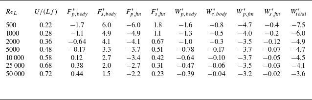


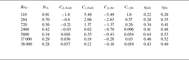


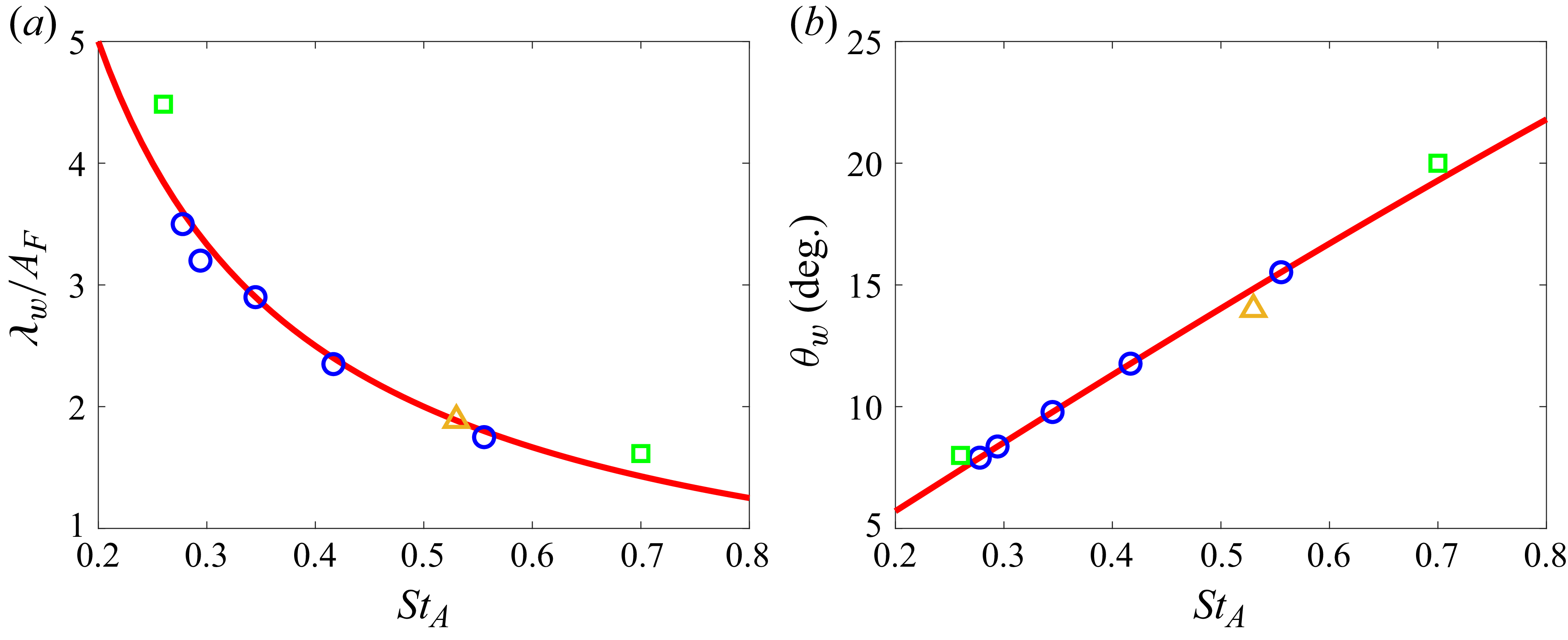


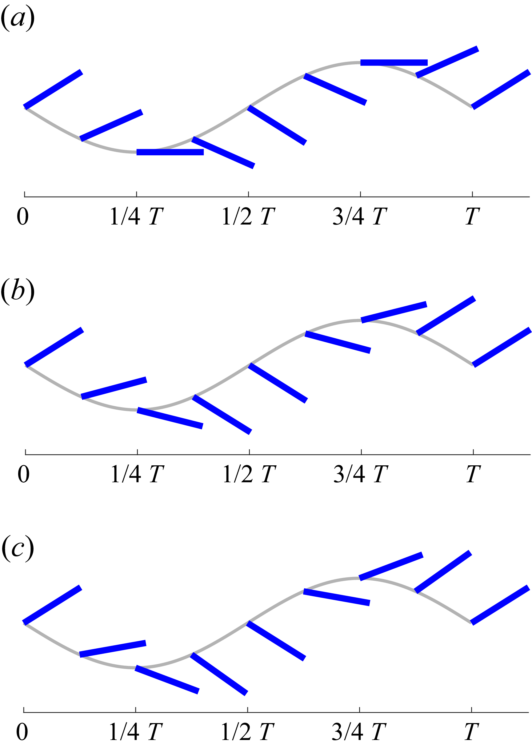


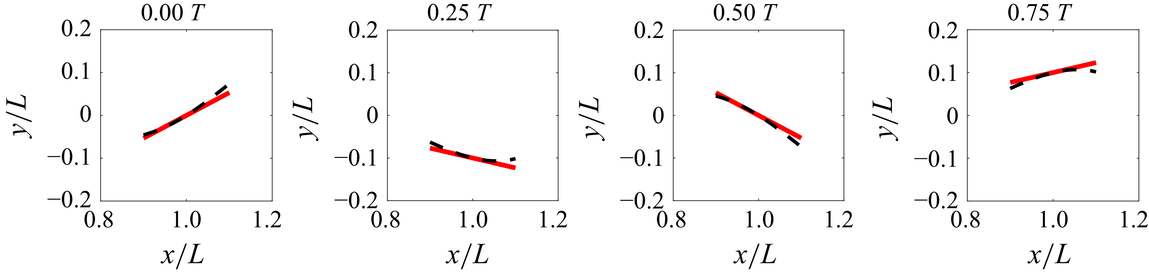
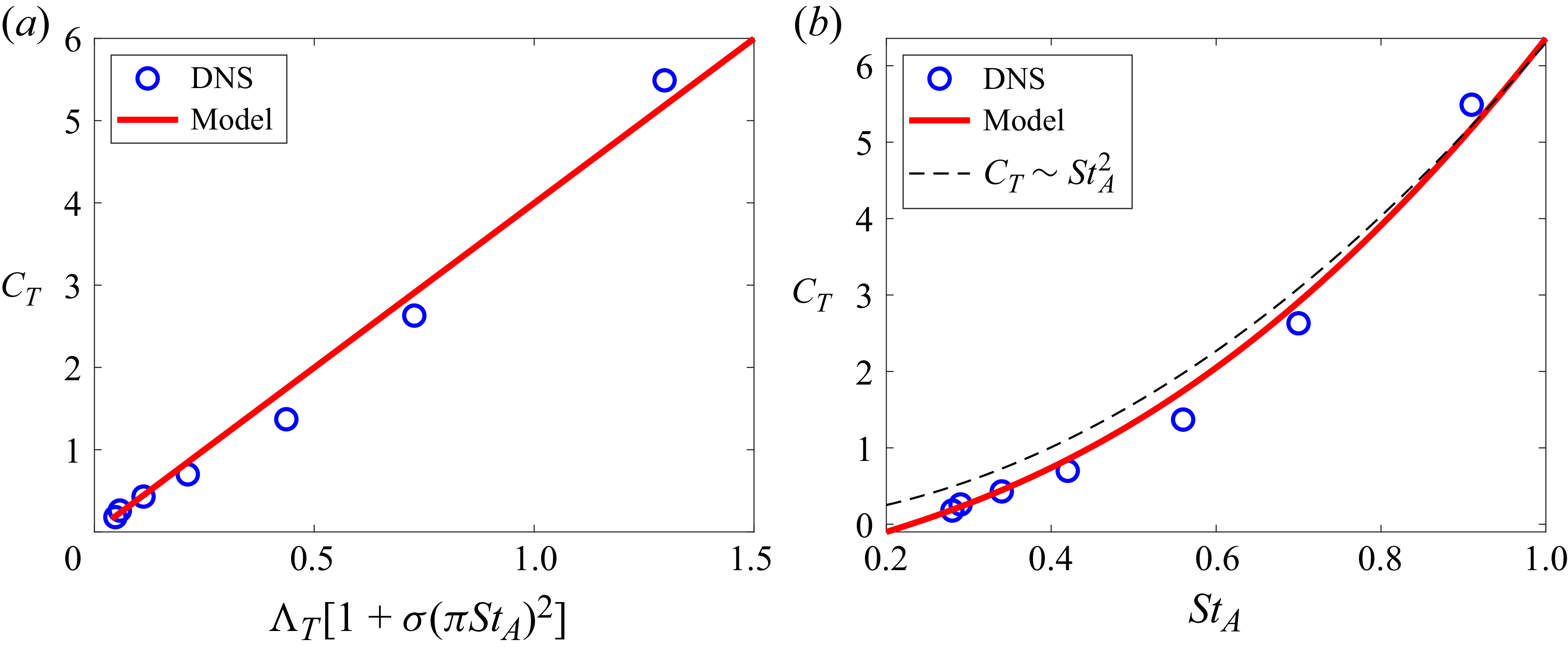


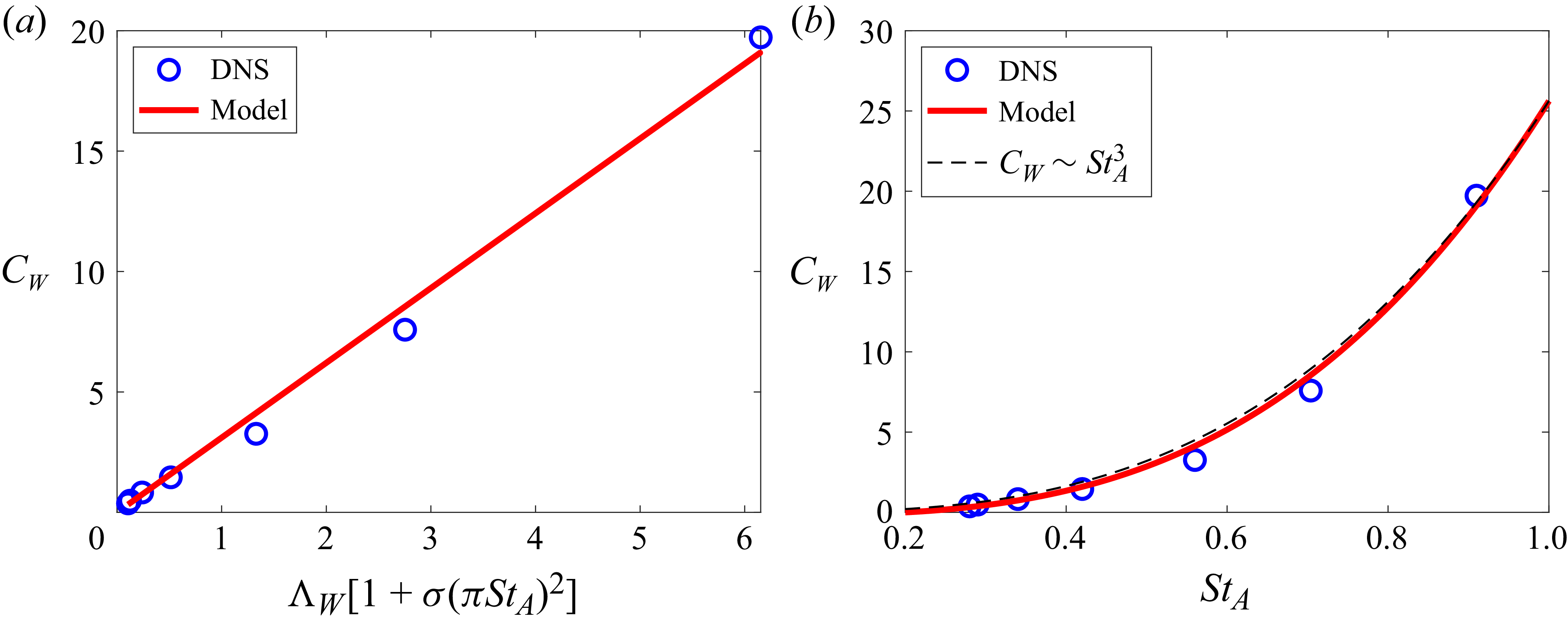

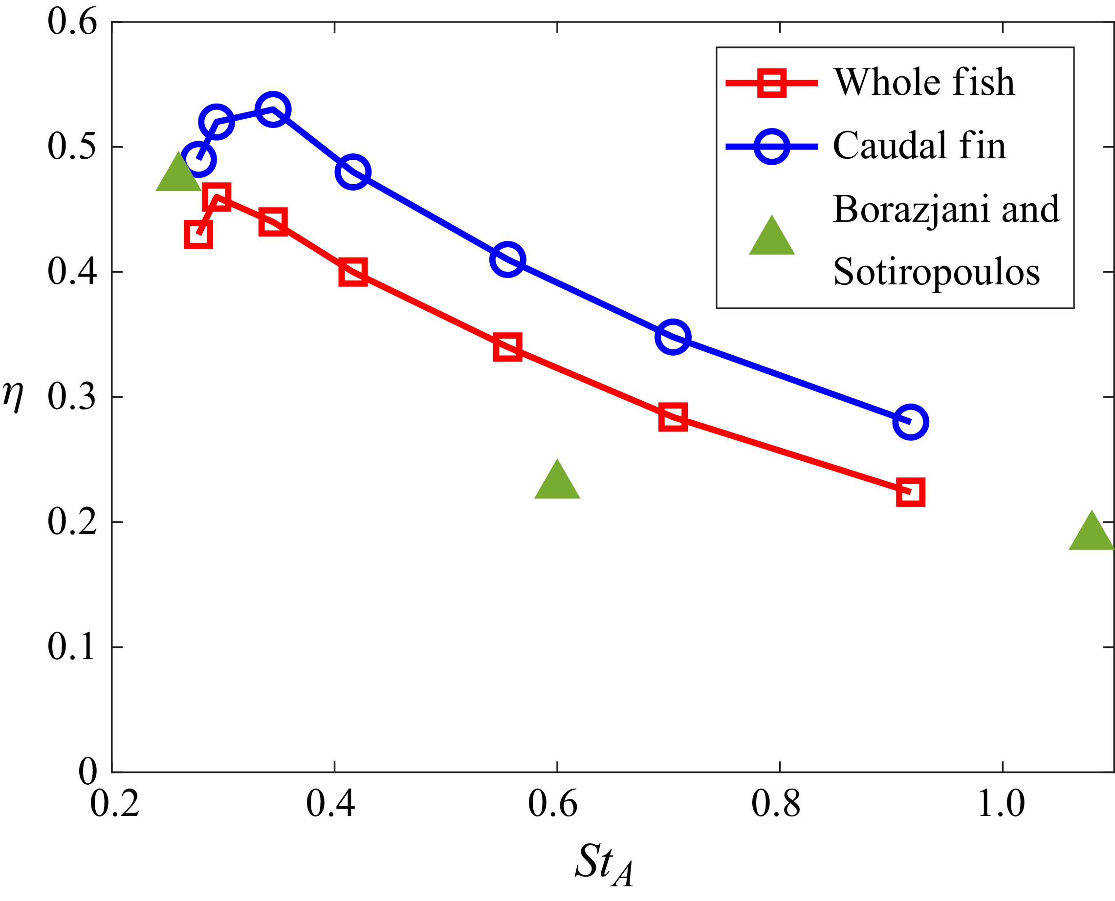
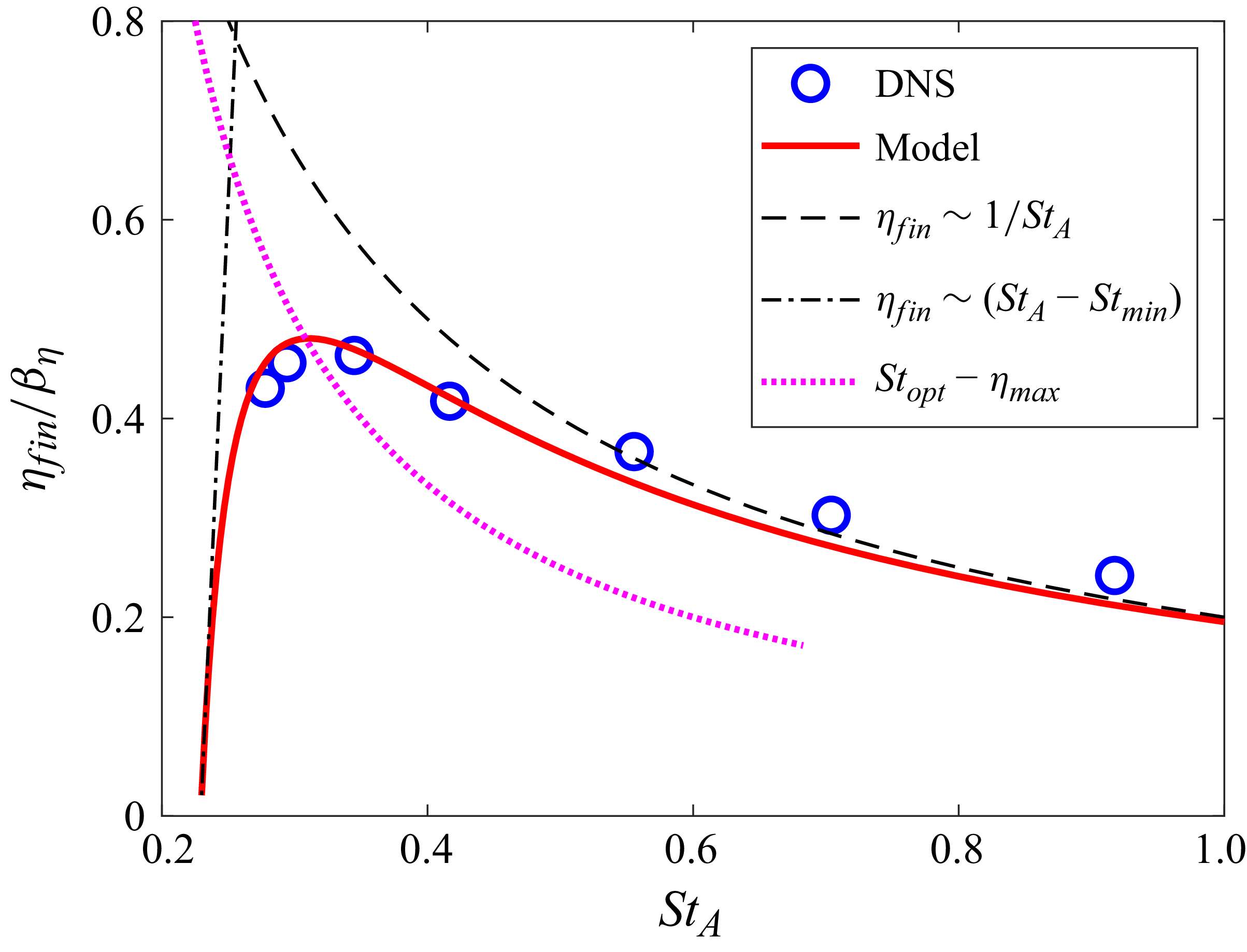


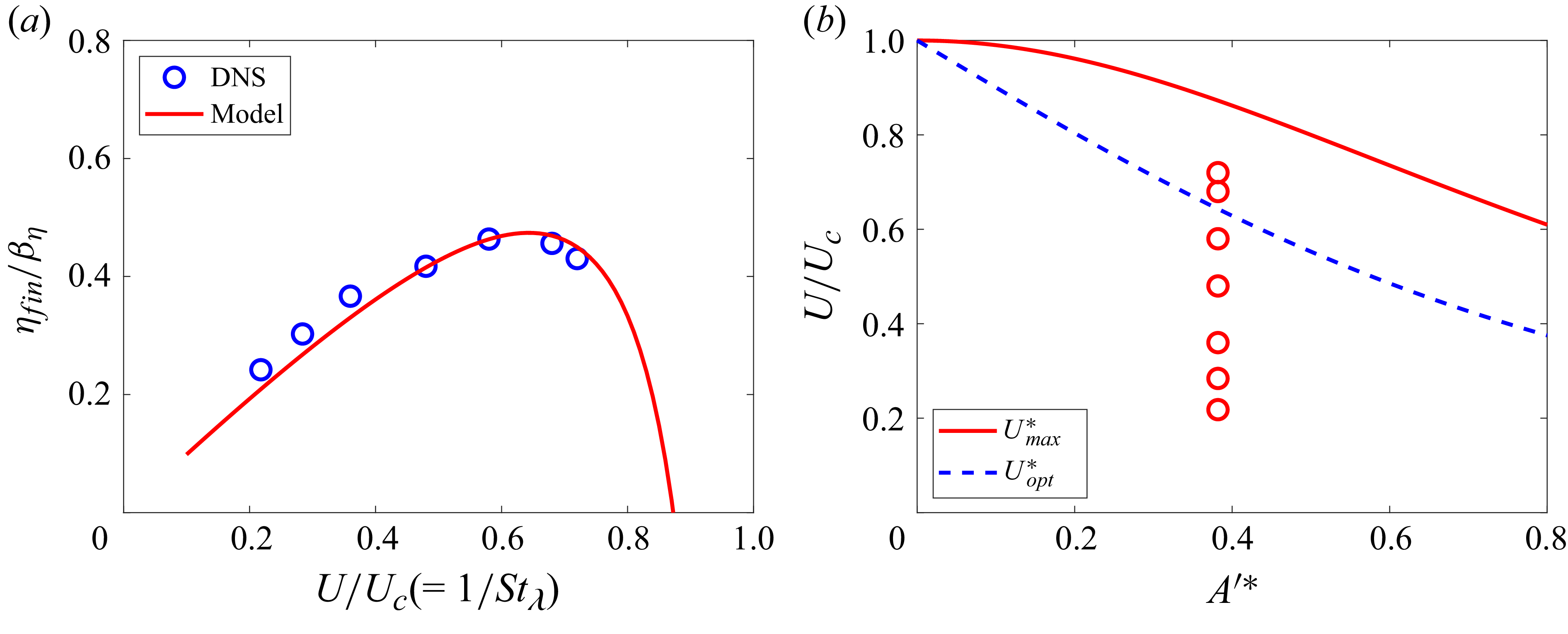


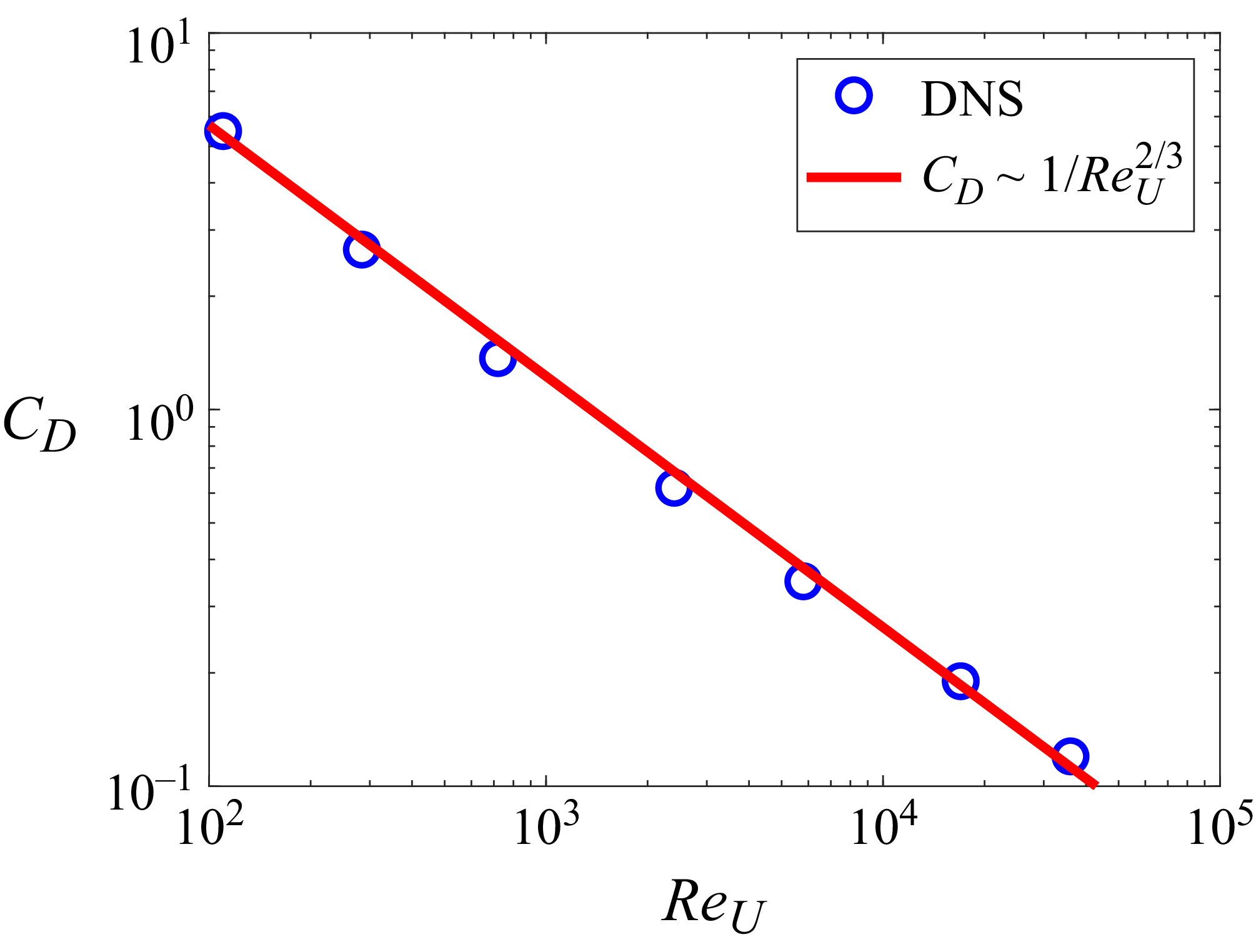
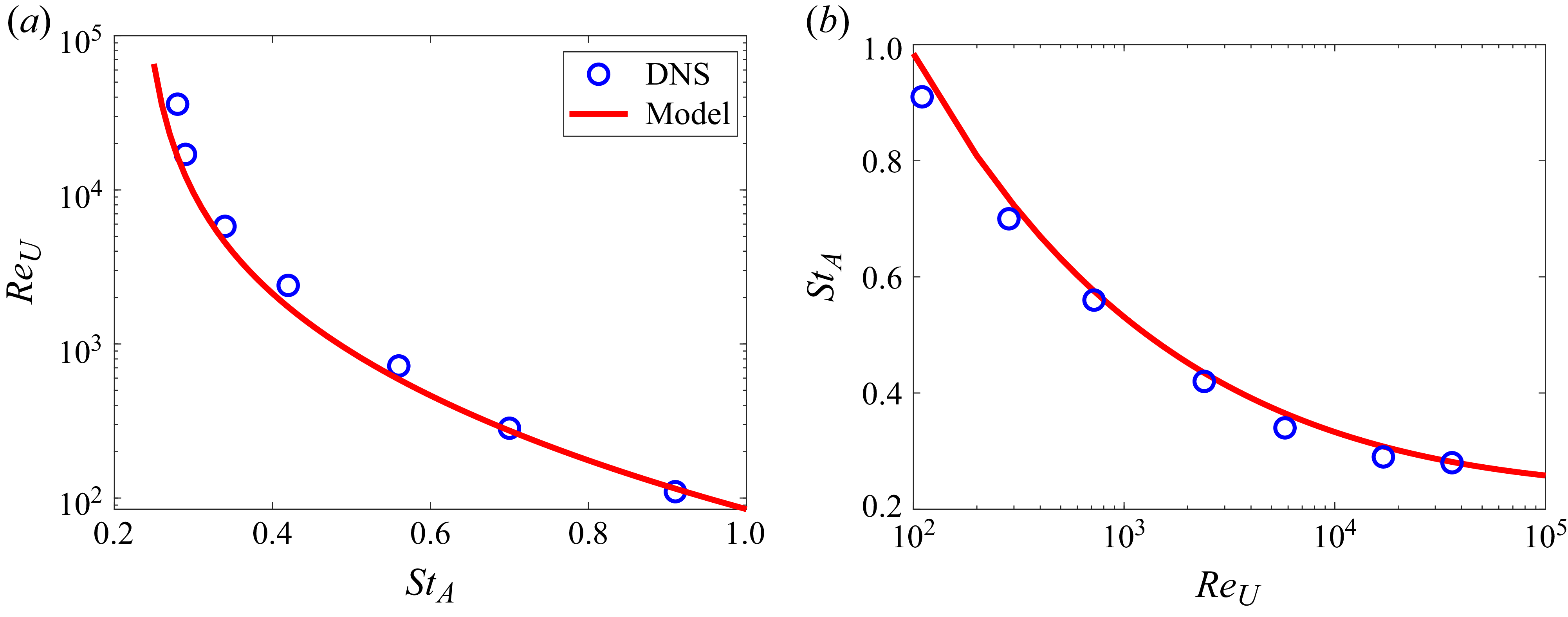


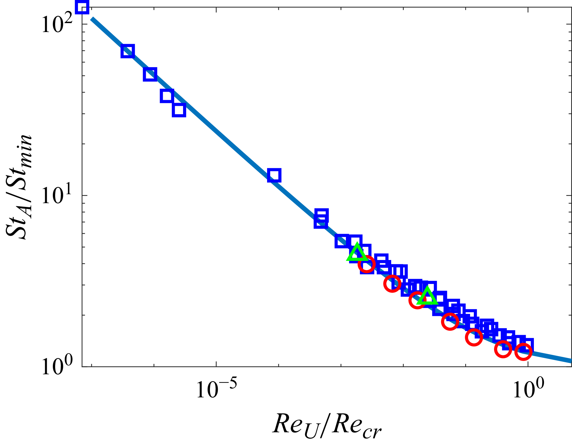


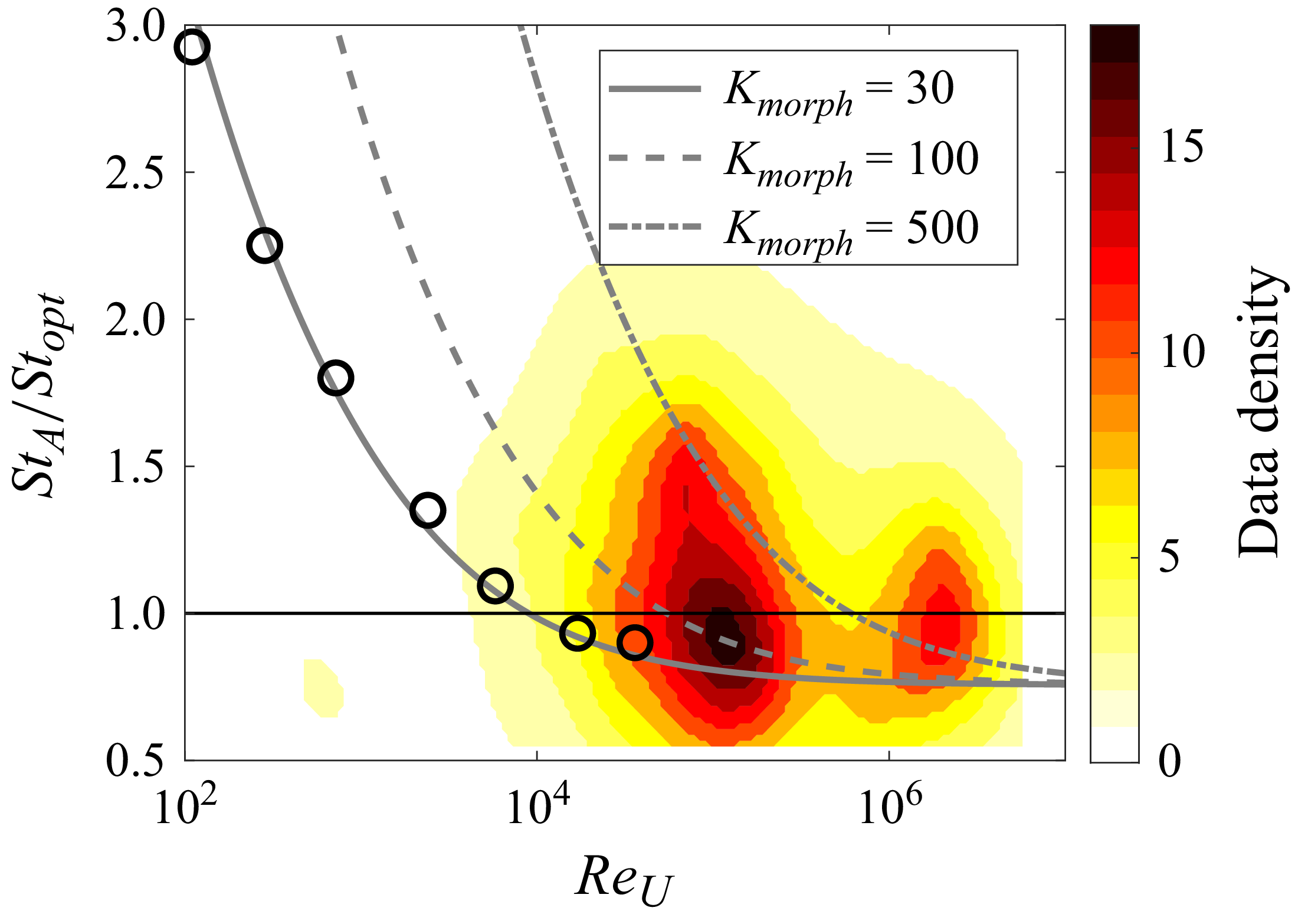


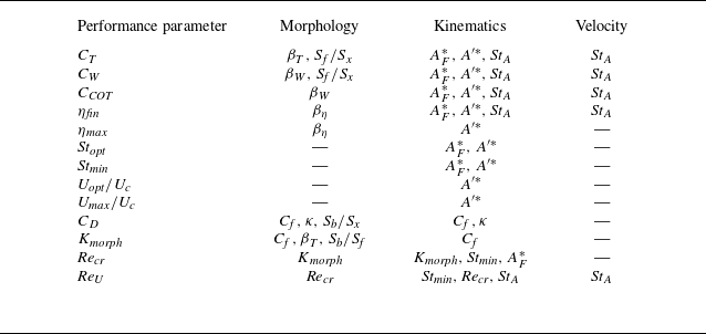
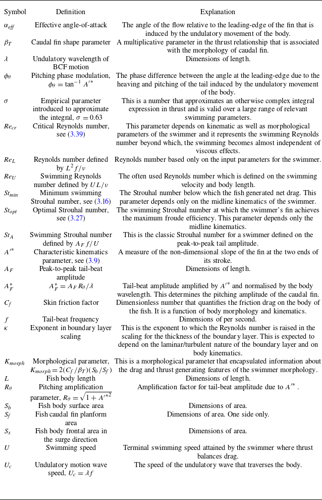


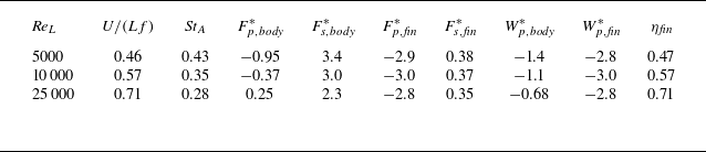


 Open access