2. The Galton–Watson process

We begin by recalling that if $i,j=1,2,\ldots$ , then $b_j=\lim_{n\to\infty} P_i(Z_n=j\mid T \gt n)$ exists independently of the initial state, and $\sum_{j=1}^\infty b_j=1$ . This defines the LCL of the process. The PGF $B(s)=\sum_{j=1}^\infty b_j s^j$ is the unique PGF solution of the functional equation

(2.1) \begin{equation} 1-B(f(s))=m(1-B(s)). \end{equation}

This result was obtained by Yaglom in 1947 assuming that $b\lt\infty$ and the general assertion was later independently published in [Reference Heathcote, Seneta and Vere-Jones6, Reference Joffe10]. See [Reference Asmussen and Hering2, Reference Athreya and Ney3] for monograph accounts, particularly the former.

Iterating (2.1) and setting $s=0$ yields the identity

\begin{equation*} \frac{1-B(f_n)}{1-f_n}=\frac{m^n}{1-f_n},\end{equation*}

from which it is obvious [Reference Heathcote, Seneta and Vere-Jones6, Reference Joffe10] that $\mu \,:\!=\, B'(1) = c^{-1}$ , i.e. the mean of the LCL equals the limit of the conditional expectation $E(Z_n\mid T \gt n)$ . We find it more convenient to work with $\mu$ . Thus, (1.1) becomes the assertion that

(2.2) \begin{equation} \mu = \mu_I \,:\!=\, 1 + \frac{b}{m(1-m)}, \end{equation}

provided that $b\lt\infty$ .

Example 2.1. We look first at the fractional linear offspring law ([Reference Athreya and Ney3, pp. 6–7] or [Reference Harris4, p. 7]) where, changing some notation from these references,

\begin{equation*}f(s) = 1 - \frac{\beta}{1-p} + \frac{\beta s}{1-ps}\end{equation*}

with $0 \lt p \lt 1$ and $0\lt\beta\lt 1-p$ . The offspring mean is $m=\beta/(1-p)^2 \lt 1$ , and $b=\beta p/(1-p)^3 = mp/(1-p)$ . It follows that

\begin{equation*} \mu_I = \frac{1-p-\beta}{(1-p)^2-\beta}\gt1. \end{equation*}

The equation $f(s)=s$ has roots $s=1$ and [Reference Harris4, p. 9]

\begin{equation*}s=s_0=\frac{1-p-\beta}{p(1-p)}.\end{equation*}

In addition, $1-f_n \sim m^n(1-s_0^{-1})$ . It follows that

\begin{equation*}\mu= (1-s_0^{-1})=\frac{1-p-\beta}{(1-p)^2-\beta},\end{equation*}

i.e. (2.2) is valid in this case. We shall see why in Section 3.

Example 2.2. A numerical counter-example to (2.2) arises from the Poisson offspring law, $f(s)={\mathrm{e}}^{-m(1-s)}$ . Bounds for $\mu$ derived in [Reference Seneta15, p. 475] are

(2.3) \begin{equation} \frac{2-m}{2(1-m)} \le \mu \le \frac{1+(1-m)^2}{(1-m)(2-m)}. \end{equation}

Clearly $b=m^2/2$ and hence

\begin{equation*}\mu_I = 1+\frac{m}{2(1-m)}=\frac{2-m}{2(1-m)},\end{equation*}

the lower bound (2.3). The proof steps in [Reference Seneta15] for (2.3) indicate that the weak inequalities there are in fact strict. This assertion is supported by [Reference Seneta15, Table II], where $\mu$ is computed to four decimal places for $m=0.1,0.2,\ldots,0.9,0.95$ and $\mu_I\lt\mu$ in all cases, although the difference is surprisingly small. We remark that the value given there for $\mu_I$ when $m=0.2$ is incorrect – it should be $1.125$ .

In both examples we have $\mu_I\le \mu$ . Might this be generally true? We shall see below that the answer is no!

A family of offspring laws embedding the fractional linear case was introduced in [Reference Sagitov and Lindo14]. This family is indexed by a primary parameter $\theta\in[-1,1]$ , along with secondary parameters. The entire family resolves into nine subfamilies, designated as cases. In all cases, explicit expressions are given for m, 2b, and the functional iterates $f_n(s)$ . We review those cases for which the offspring law is subcritical.

Case 1 has $b\lt\infty$ in only the boundary case $\theta=1$ and it is the linear fractional offspring law. The secondary parameters in [Reference Sagitov and Lindo14] are $a=(1-p)/\beta$ and $d=(1-p)p/(1-p-\beta)$ . We say no more about this case. The other relevant cases specify a parameter $a\in(0,1)$ , which turns out to be the offspring mean, m. Hence we replace a in [Reference Sagitov and Lindo14] with m.

Example 2.3. Case 7 has $\theta\in(0,1)$ and a parameter $A\gt1$ . There is a second parameter q, which here must have the value $q=1$ to ensure that $\sum p_j=1$ . Setting $p=A^{-1}$ , the functional iterates have the form

\begin{align*} f_n(s) & = A - [m^n(A-s)^{-\theta}+(1-m^n)(A-1)^{-\theta}]^{-1/\theta} \\ & = A[1-(m^n(1-ps)^{-\theta} +(1-m^n)(1-p)^{-\theta})^{-1/\theta}]. \end{align*}

In addition,

\begin{equation*}\frac{2b}{m(1-m)} = \frac{1+\theta}{A-1} = (1+\theta)\frac{p}{1-p}.\end{equation*}

Hence,

\begin{equation*}\mu_I = 1 + \frac{1+\theta}{2}\cdot\frac{p}{1-p}.\end{equation*}

Setting $s=0$ , some manipulation with the first form of $f_n(s)$ yields

\begin{align*} f_n & = A-(A-1)[1-m^n(1-(1-p)^{\theta})]^{-1/\theta} \\ & = 1-\theta^{-1} (A-1) m^n[1-(1-p)^\theta](1+o(1)). \end{align*}

It follows that

\begin{equation*}\mu = \frac{\theta}{A-1} \cdot \frac{1}{1-(1-p)^\theta} = \frac{\theta p}{(1-p)(1-(1-p)^\theta)},\end{equation*}

manifestly different to $\mu_I$ .

Further manipulation reveals that

\begin{equation*}B(s) = \frac{1-(1-ps)^\theta}{1-(1-p)\theta} \cdot \bigg(\frac{1-p}{1-ps}\bigg)^\theta,\end{equation*}

the PGF of the sum of two independent random variables, $S_{p,\theta}+N_{p,\theta}$ , where $S_{p,\theta}$ has a power-series law generated by the Sibuya law whose PGF is $1-(1-s)^\theta$ , and $N_{p,\theta}$ has a negative binomial law.

Example 2.4. For Case 8 in [Reference Sagitov and Lindo14], the relevant parameter choices are $\theta=0$ , $q=1$ , and $A\gt1$ , and then

(2.4) \begin{equation} f_n(s) = A-(A-1)^{1-m^n}(A-s)^{m^n} \end{equation}

with $2b/m(1-m) = (A-1)^{-1}$ . It follows that

\begin{equation*}\mu_I = 1 + \frac{1}{2(A-1)} = \frac{2-p}{2(1-p)},\end{equation*}

the same algebraic form as for the Poisson case.

Setting $s=0$ in (2.4) yields

\begin{align*} f_n & = (A-1)\bigg[\bigg(\frac{A}{A-1}\bigg)^{m^n}-1\bigg] = (A-1) \big[(1-p)^{-m^n}-1\big] \\ & = (A-1)m^n(-\log(1-p))(1+o(1)), \end{align*}

whence

\begin{equation*}\mu = [(A-1)(-\log(1-p))]^{-1} = \frac{p}{1-p}(-\log(1-p))^{-1}.\end{equation*}

Again, $\mu_I\ne \mu$ .

We can compare $\mu_I$ and $\mu$ by ignoring the common factor $1-p$ and observing that

\begin{equation*} \frac{p}{-\log(1-p)} = \frac{1}{1+p/2+p^2/3+\cdots} \gt \frac{1}{1+(p/2)(1+p+p^2+\cdots)}=\frac{1-p}{1-p/2}. \end{equation*}

But

\begin{equation*}1-p/2-\frac{1-p}{1-p/2} = \frac{p^2/4}{1-p/2}\gt 0,\end{equation*}

and we conclude that for this case, $\mu_I\gt\mu$ . Hence there is no general order relation between $\mu$ and $\mu_I$ . Numerical calculation shows for this case that the relative error $\mu_I/\mu-1$ is within $0.04$ if $m\in(0, 0.5]$ , and it increases quite quickly if $m\in[0.6,1)$ , e.g. it is 0.113 if $m=0.6$ .

Finally, calculation shows that the LCL has the log-series law,

\begin{equation*} B(s)=\frac{\log(1-ps)}{\log(1-p)}.\end{equation*}

Example 2.5. Our last example, Case 9 in [Reference Sagitov and Lindo14], has $\theta\in(-1,0)$ , $A\gt1$ , and $q=1$ . Writing $\zeta=-\theta$ , the functional iterate is $f_n(s)=A-[m^n(A-s)^\zeta+(1-m^n)(A-1)^\zeta]^{1/\zeta}$ and $b/m(1-m)=(1-\zeta)/(A-1)$ . Hence,

\begin{equation*}\mu_I = \frac{2A-1-\zeta}{2(A-1)} = \frac{2-(1+\zeta)p}{2(1-p)}.\end{equation*}

Setting $s=0$ we obtain

\begin{equation*}1-f_n = \zeta^{-1}(A-1)m^n\bigg[\bigg(\frac{A}{A-1}\bigg)^\zeta-1\bigg](1+o(1)),\end{equation*}

and hence

\begin{equation*}\mu = \frac{\zeta p}{1-p}((1-p)^{-\zeta}-1)^{-1} \ne \mu_I.\end{equation*}

Numerical calculation suggests that $\mu_I\gt\mu$ . We shall confirm this in Section 3.

The LCL is a power-series law generated from a Sibuya law,

\begin{equation*}B(s) = \frac{1-(1-ps)^\zeta}{1-(1-p)^\zeta}.\end{equation*}

We end this section by recalling the upper bound for $\mu$ derived in [Reference Agresti1] using bounding linear-fractional offspring laws.

Theorem 2.1. If $b\lt\infty$ , then

(2.5) \begin{equation} \mu \lt 2\mu_I-1 = 1+\frac{2b}{m(1-m)}. \end{equation}

Proof. A double differentiation of (2.1) yields $2b\mu+m^2 B''(1)=mB''(1)$ . Observing that, in obvious notation, $B''(1)=\sigma^2_B+\mu^2-\mu$ , division by $\mu$ yields

\begin{equation*} 2b=m(1-m)\big(\sigma^2_B+\mu-1\big)\gt m(1-m)(\mu-1),\end{equation*}

and (2.5) follows.

This simple proof shows that the weak inequality in [Reference Agresti1, p. 331] is in fact strict, and that (2.5) is equivalent to the crudest possible lower bound of $\sigma^2_B$ . Can (2.5) be refined?

The presentation in [Reference Imomov and Murtazaev8] is in terms of the non-critical case $m\ne 1$ . That the subcritical case is fundamental follows because, as is known, it subsumes the supercritical case in matters of ultimate extinction. Let $\overline{f}(s)$ be an offspring-number PGF satisfying $\overline{f}(0)\gt 0$ and $\overline{f'}(1)\in(1,\infty]$ . Then $\overline{f}(s)=s$ has a unique solution $q\in(0,1)$ , the probability that the associated GWP $(\overline{Z}_n\,:\,n\ge0)$ with $\overline{Z}_1=1$ hits the zero state. The Sevast’yanov transformation $f(s)=\overline{f}(qs)/q$ determines a subcritical offspring-number law: $m=\overline{f'}(q) \lt 1$ (denoted by $\beta$ in [Reference Imomov and Murtazaev8]). Clearly $f_n(s)=\overline{f}_n(qs)/q$ , hence $\overline{f}_n\,:\!=\, \overline{f}_n(0)=qf_n \uparrow q$ .

A natural definition of a supercritical Kolmogorov constant is $ \overline{c}=\lim_{n\to\infty} m^{-n}(q-\overline{f}_n)=qc$ , where c is the Kolmogorov constant for the induced subcritical GWP. Note that $\overline{c}$ is denoted by $\mathcal{K}_q$ in [Reference Imomov and Murtazaev8].

Defining $\overline{b}=\frac{1}{2}\overline{f''}(q) =b/q$ (denoted by $b_q$ in [Reference Imomov and Murtazaev8]), [Reference Imomov and Murtazaev8, Theorem 2.1] asserts that

\begin{equation*} \overline{c}=\frac{ q}{1+ \overline{b}/m(1-m)}= q\bigg(1+ \frac{b}{m(1-m)}\bigg)^{-1}.\end{equation*}

It follows that examples/counter-examples for the supercritical case correspond to any, such as those above, constructed from a subcritical f(s) whose domain of holomorphy extends sufficiently far beyond the unit disc as to have a fixed point in $(1,\infty)$ . For example, the Poisson offspring-number laws.

3. The Markov branching process

We begin by recalling that the subcritical MBP has a stationary measure $(\pi_j\,:\,j\ge 1)$ whose generating function is

(3.1) \begin{equation} \pi(s) = \int_0^s\frac{1-m}{f(u)-u}\,{\mathrm{d}} u, \end{equation}

where f(s) is the offspring PGF of the MBP. Note that this stationary measure is independent of the split rate and it is unique up to scaling. The scaling chosen for (3.1) is the most natural in the sense that the PGF of the LCL is

(3.2) \begin{equation} \widehat B(s) \,:\!=\, \lim_{t\to\infty}E_i\big(s^{Y_t}\mid\widehat T\gt t\big) = 1-{\mathrm{e}}^{-\pi(s)}. \end{equation}

See [Reference Harris4] for the most explicit statements and [Reference Athreya and Ney3] for a simple proof based on the fact that, for each constant $\delta > 0 $ , the so-called discrete skeleton $(Y_{\delta n}\,:\,n\ge0)$ is a GWP. It follows from (3.1) and (3.2) that

(3.3) \begin{equation} \widehat\mu = \lim_{s\uparrow 1}\frac{1-\widehat B(s)}{1-s} = \lim_{s\uparrow 1}{\mathrm{e}}^{-\pi(s)-\log(1-s)} = \exp\bigg[{-}\int_0^1\bigg(\frac{1-m}{f(s)-s}-\frac{1}{1-s}\bigg)\,{\mathrm{d}} s\bigg]. \end{equation}

On the other hand, it follows from Galton–Watson theory that $\widehat\mu=\widehat c^{-1}$ and hence (1.2) is equivalent to the assertion that

(3.4) \begin{equation} \widehat\mu=\widehat\mu_I\,:\!=\,1+\frac{b}{1-m}. \end{equation}

We now show that (3.4) follows from (2.2). Recall that the mean population size of the MBP is $m_t=E_1(Y_t)={\mathrm{e}}^{-\nu t}$ , where $\nu=a(1-m)$ , the negative of the Malthusian parameter. Also, let $b_t=\frac{1}{2} E_1[Y_t(Y_t-1)]$ . It follows from (2.2) applied to the discrete skeleton that, for any $t\gt 0$ ,

\begin{equation*} \widehat\mu_I= 1+ \frac{b_t}{m_t(1-m_t)}.\end{equation*}

A long-known result is that [Reference Harris4, p. 103]

\begin{equation*}\mathrm{Var}(Y_t \mid Y_0=1) = \frac{f''(1)-m+1}{1-m}m_t(1-m_t) = \bigg(\frac{2b}{1-m}+1\bigg)m_t(1-m_t).\end{equation*}

However, the variance equals $2b_t+m_t(1-m_t)$ and hence

\begin{equation*} \frac{b_t}{m_t(1-m_t)}\equiv \frac{b}{1-m},\end{equation*}

and the expression in (3.4) for $\widehat\mu_I$ follows.

It is observed in [Reference Sagitov and Lindo14, Section 7] that the $\theta$ -offspring laws arise as discrete skeletons of certain MBPs. An alternative approach to constructing examples of LCLs is taken in [Reference Pakes12, Reference Tchorbadjieff, Mayster and Pakes17] by finding criteria which ensure that a PMF $(b_j\,:\,j\ge 1)$ is the LCL of a subcritical MBP, in fact an uncountable family of MBPs. Examples in these papers provide counter-examples to (3.4).

Example 3.1. Choose a constant ${\lambda}\in(0,1)$ , set $\theta= {\lambda}{\mathrm{e}}^{-{\lambda}}$ , and let C(z) be the Cayley tree-counting function, i.e. the solution of the functional equation $C=z{\mathrm{e}}^C$ , where $z\ge 0$ , which satisfies $0\le C(z)\le{\mathrm{e}}^{-1}$ . The Cayley function is related to the better-known principal Lambert function W(z) by $C(z)=-W(-z)$ . It is shown in [Reference Tchorbadjieff, Mayster and Pakes17, Section 3] that $\widehat B(s)={\lambda}^{-1} C(\theta s)$ is the PGF of the LCL of MBPs whose offspring PGF is

\begin{equation*} f(s)=[1-(1-m)(1+{\lambda})]s+(1-m)s[{\lambda} \widehat B(s)+1/\widehat B(s)],\end{equation*}

where the offspring mean m is chosen subject to the constraint

\begin{equation*}\frac{2 {\lambda}}{1+{\lambda}}\le m \lt 1.\end{equation*}

The derivative identity

\begin{equation*} C'(z)=\frac{C(z)}{z(1-C(z))}\end{equation*}

leads to the evaluations

\begin{equation*} \widehat\mu=\frac{1}{1-{\lambda}}\lt \widehat\mu_I=\frac{1}{2}\bigg[1+ \frac{1}{(1-{\lambda})^2}\bigg].\end{equation*}

Example 3.2. Choosing constants $p\in(0,1)$ and $\alpha\in(0,1]$ , it is shown in [Reference Pakes12] that

\begin{equation*} \widehat B(s)= 1-\frac{1-s}{(1-ps)^\alpha}\end{equation*}

generates an LCL. If $\alpha=1$ , then this law is a shifted geometric distribution. See Section 5 for more on this case. It is obvious that $\widehat\mu=(1-p)^{-\alpha}$ .

The corresponding offspring probabilities for $j\ge 2$ , defining $\rho=(1-\alpha)p/(1-\alpha p)$ , are

\begin{equation*} p_j =\frac{1-m}{1-\alpha p}(1-\rho) (p-\rho) \rho^{j-2},\end{equation*}

where the offspring mean must satisfy

\begin{equation*} 1- \frac{(1-\alpha p)^2}{1- \alpha p^2}\le m \lt 1.\end{equation*}

Observing that $\sum_{j\ge 2} j(j-1) \rho^{j-2}=2(1-\rho)^{-3}$ , some algebra leads to

\begin{equation*} \widehat\mu_I=\frac{1-(1-\alpha)p}{1-p}.\end{equation*}

This equals $\widehat\mu$ if $\alpha=1$ , but not if $\alpha \lt 1$ .

We end this section by showing that $\widehat\mu_I$ always bounds $\widehat\mu$ from above, and that this implies a lower bound for the variance $\widehat\sigma^2$ of the LCL.

Proof. For (i), referring to (3.3), a Taylor expansion yields

\begin{equation*}f(s)=1-m(1-s)+b(s)(1-s)^2,\end{equation*}

where $\frac{1}{2} f''(s)\lt b(s)\le b$ , and $b(s)\equiv b$ if and only if f(s) is a quadratic function. Hence

\begin{equation*}\frac{1-m}{f(s)-s} = [(1-s)(1+(1-s)b(s)/(1-m))]^{-1},\end{equation*}

i.e.

\begin{equation*}0 \lt \frac{1}{1-s} - \frac{1-m}{f(s)-s} = \frac{b(s)/(1-m)}{1+(1-s)b(s)/(1-m)} \le \frac{b/(1-m)}{1+(1-s)b/(1-m)}.\end{equation*}

Hence, the exponent in (3.3) is bounded above by

\begin{equation*}\int_0^1\frac{b/(1-m)}{1+ub/(1-m)}\,{\mathrm{d}} u = \log\bigg(1+\frac{b}{1-m}\bigg),\end{equation*}

i.e. $\widehat\mu \le 1+b/(1-m)=\widehat\mu_I$ .

For (ii), let $(b_j\,:\,j\ge 1)$ denote an arbitrary PMF satisfying $b_1\gt 0$ and having the PGF $\widehat B(s)$ . Then the function $\beta(s)\,:\!=\, (1-\widehat B(s))/\widehat B'(s)$ has a power series representation $\beta(s)=\sum_{j=0}^\infty \beta_j s^j$ converging in the open unit disc, and $\beta_1=-1-2b_2/b_1\lt0$ . Then $(b_j)$ is the PMF of the LCL of a subcritical MBP if and only if $\beta_j \ge 0$ for $j\ge 2$ , and the offspring mean satisfies

\begin{equation*} 1+1/\beta_1\le m \lt 1.\end{equation*}

If these conditions are satisfied, then the offspring-number PGF is $f(s) = s+(1-m)\beta(s)$ and

\begin{equation*}\widehat\mu_I = 1 + \frac{1}{2}\beta''(1) = 1 + \frac{\widehat B''(1)}{2 \widehat\mu}.\end{equation*}

Since $\widehat B''(1)=\widehat\sigma^2-\widehat\mu+\widehat\mu^2$ , we see that

\begin{equation*} \frac{\widehat\sigma^2-\widehat\mu-\widehat\mu^2}{2\widehat\mu}= \widehat\mu_I-\widehat\mu,\end{equation*}

and (3.6) follows from (3.5).

A consequence of Theorem 3.1(i) is that if $(Z_n)$ is a GWP embeddable in a subcritical MBP, then $\mu \le \mu_I$ with equality if and only if the embedding MBP is a generalised linear birth and death process. This contingency implies that the embedded GWP has a linear fractional offspring-number law. We conclude therefore, that (1.3) is an equality only for Example 2.1.

4. Approximating $\mu$

Several papers were published around 1970 concerned with computable bounds for quantities associated with the distribution of the extinction time t of the GWP [Reference Agresti1, Reference Heathcote and Seneta5, Reference Pollak13, Reference Seneta16]. As observed in Section 1, an upper bound of the form $\mu \le \mu_n+B_n$ can be distilled from bounds derived in [Reference Pollak13, Reference Seneta16]. Assume $b \lt\infty$ and let $n\to\infty$ in the starred inequality on [Reference Seneta16, p. 673]. Then, replacing h there with n, we obtain the evaluation of $B_n$ as

(4.1) \begin{equation} B_n(S) \,:\!=\, \frac{b m^n}{(1-m) f'(f_n)}. \end{equation}

Pollak [Reference Pollak13] derived bounds for c assuming that the third-order factorial moment $f'''(1)\lt\infty$ . His lower bound depends only on b. Written as an upper bound for $\mu$ yields his evaluation of $B_n$ as

(4.2) \begin{equation} B_n(P) \,:\!=\, \frac{b m^{n-1}}{(1-m)[1-bm^{-1}(1-f_n)]}. \end{equation}

Choosing a desired error $\varepsilon\in(0,1)$ , we achieve the bounds $0\lt\mu-\mu_n \le\varepsilon$ by choosing n such that $B_n\le \varepsilon$ . Observe that the denominators in (4.1) and (4.2) increase with n. Recalling that $f_n \uparrow1$ , we see for both cases that $B_n \ge bm^{n-1}/(1-m)$ . It follows that an absolute minimum value required for n is

\begin{equation*}n \ge n_{\ell} = 2+ \bigg\lfloor\frac{\log(b/\varepsilon)+\log(1-m)^{-1}}{\log m^{-1} }\bigg\rfloor. \end{equation*}

Observe next that $B_n(S)\le \varepsilon$ if

\begin{equation*} n \ge \frac{\log[b/(\varepsilon(1-m)f'(f_n))]}{\log m^{-1}}. \end{equation*}

Values of n satisfying this criterion are obtained by choosing a small natural number k, and then

\begin{equation*}n \ge n_{Sk} \,:\!=\, \bigg(1+\bigg\lfloor \frac{\log[b/\varepsilon (1-m)f'(f_k)]}{\log m^{-1}}\bigg\rfloor\bigg)\vee k.\end{equation*}

The simplest choice is $k=1$ , in which case $f'(f_1)=f'(p_0)$ .

Recall for the Poisson case that we have $b=m^2/2$ . In addition, $p_0={\mathrm{e}}^{-m}$ and $f'(p_0)=m\exp[-m(1-{\mathrm{e}}^{-m})]$ . Hence

\begin{equation*} n_{S1}= \bigg\lfloor\frac{\log(2/\varepsilon) -\log(1-m) +m(1-{\mathrm{e}}^{-m})}{\log m^{-1}}\bigg\rfloor. \end{equation*}

A similar strategy applied to (4.2) yields the condition

\begin{equation*} n \ge n_{Pk}= \bigg(1+\bigg\lfloor\frac{\log[b/\varepsilon(1-m)(1-bm^{-1}(1-f_k))]}{\log m^{-1}}\bigg\rfloor\bigg)\vee k.\end{equation*}

For the Poisson case with $k=1$ , we have

\begin{equation*} n_{P1}=\bigg\lfloor\frac{\log(2/\varepsilon)-\log(1-m)-\log(1-(m/2)(1-{\mathrm{e}}^{-m}))}{\log m^{-1}}\bigg\rfloor. \end{equation*}

Defining $\phi(u)=-\log(1-u/2)$ for $u\in(0,1)$ , it is easily checked that $\phi(u)\lt u$ , implying that $n_{S1}\ge n_{P1}$ .

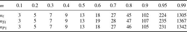
Values of $n_\ell$ , $n_{S1}$ , and $n_{P1}$ for the Poisson case and $\varepsilon=10^{-4}$ (following [Reference Seneta15]) are displayed in Table 1. We see that there is little relative difference between $n_{S1}$ and $n_{P1}$ if $m \le 0.99$ , and that $n_{S1}\ge n_{P1}$ , with equality if $m \le 0.5$ and significant difference only if m is very close to unity. In addition, neither $n_{S1}$ nor $n_{P1}$ exceed $n_\ell$ to any marked degree unless m is close to unity.

Table 1.

Minimum values of n required to achieve $\mu-\mu_n \le 10^{-4}$ for Poisson offspring-number laws.

Very similar outcomes occur for the geometric offspring-number law $f(s)=(1+m-ms)^{-1}$ . Here, we know that $\mu=(1-m)^{-1}$ . Values of $n_{S1}$ and $n_{P1}$ are identical if $m\le 0.7$ , differ by at most 2 if $0.8\le m\le 0.95$ , and differ by 12 if $m=0.99$ . There is little difference, 3 at most, between $n_{S1}$ or $n_{P1}$ and $n_\ell$ if $m\le 0.8$ .

Returning to the Poisson case, we mention that Pollak’s upper bound $1.2244=1/0.8167$ when $m=0.3$ [Reference Pollak13, Table 1] is less than the numerical value $\mu=1.2327$ in [Reference Seneta15, Table II]. The latter value is incorrect. We see from Table 1 that $n_{S1}=n_{P1}=7$ , and computation yields $\mu_6=1.222\,257$ , $\mu_7=1.222\,366$ , $\mu_8=1.222\,399$ and $\mu_9=1.222\,409$ . Thus, to within $10^{-4}$ , $\mu=1.2224$ , consistent with Pollak’s bound. In addition, this degree of accuracy is achieved by $\mu_7$ , as designed, but not by $\mu_6$ .

5. Final remarks

We conclude by discussing two matters from [Reference Imomov and Murtazaev8]. The identity (2.2) is essentially the subcritical version of [Reference Imomov and Murtazaev8, Theorem 1.2]. This follows from [Reference Imomov and Murtazaev8, Lemma 2.2], which asserts that a function $\Delta(s)$ defined in the first display on p. 933 is constant-valued. In our notation (see [Reference Imomov and Murtazaev8, (2.8)]),

\begin{equation*} \Delta(s)=\frac{\mu}{1-B(s)}- \frac{1}{1-s}. \end{equation*}

[An aside: It follows that $\Delta(s)=\sum_{j\ge 1} \Delta_j s^j$ , where $\Delta_j=\mu u_j-1$ and $(u_j)$ is a renewal sequence such that $u_j\to \mu^{-1}$ .] Specifically, [Reference Imomov and Murtazaev8, Lemma 2.2] is asserting that $\Delta(s)\equiv \gamma$ . This has consequences for the allowable form of f(s), as we now explain.

Defining $p=\gamma/(1+\gamma)\in(0,1)$ , [Reference Imomov and Murtazaev8, Lemma 2.2] asserts that

\begin{equation*} B(s)=1-\mu(1-p) \frac{1-s}{1-ps}. \end{equation*}

But $B(0)=0$ , whence $\mu(1-p)=1$ , i.e.

\begin{equation*} B(s)=s\frac{1-p}{1-ps},\end{equation*}

the PGF of a shifted geometric law, mentioned in Example 3.2.

Conversely, if $p\in (0,1)$ and B(s) has this form, then it follows from the functional equation that it corresponds to offspring PGFs having the form

\begin{equation*} f(s\,;\,m)=\frac{1-m+(m-p)s}{1-mp-p(1-m)s}.\end{equation*}

This specifies the linear-fractional offspring laws, and [Reference Imomov and Murtazaev8, Theorem 2.1 and Lemma 2.2] are valid for these laws.

It follows from our counter-examples that $\Delta(s)$ is not, in general, constant-valued. The algebraic detail in [Reference Imomov and Murtazaev8] is correct up to the display following [Reference Imomov and Murtazaev8, (2.35)]. The next display giving the desired contradiction is not correct. It results from incorrect use of the algebra of asymptotic equivalence. To illustrate the error, let $u(s)\equiv 1$ and $v(s)=s=1-(1-s)$ . If $\nu$ is any real number then, as $s\to1$ , $ u(s) \sim (v(s))^\nu = (1-(1-s))^\nu=1-\nu(1-s)(1+o(1))$ . We emphasise that this is valid for all real $\nu$ , but it is invalid to equate the coefficients of $1-s$ on each side of the asymptotic equivalence, i.e. to adduce the conclusion $\nu=0$ . This is exactly the error committed in going to the second unlabelled display in [Reference Imomov and Murtazaev8].