


«Now, here, you see, it takes all the running you can do, to keep in the same place. If you want to get somewhere else, you must run at least twice as fast as that!»
Lewis Carroll, Through the Looking Glass (1900) p. 39
1. INTRODUCTION
The neoclassical growth model is the basic theoretical framework to study economic growth. The so-called convergence hypothesis implies that as poorer countries grow faster than richer countries, international income levels tend to converge (Ray Reference Ray1998; Jones Reference Jones2001). This is also the idea behind Lewis Carroll's «Red Queen race»: if poor countries would like to reach the income levels of richer countries, they must grow faster than these rich countries to whom they want to draw nearer. The modern literature on economic growth, besides considering factors that influence the accumulation of resources and the efficiency with which they are used, includes institutions as key explanatory variables. Institutions can provide legal certainty and foster the development of human creativity (North Reference North1990; Acemoglu et al. Reference Acemoglu, Johnson, Robinson, Aghion and Durlauf2005; Greif Reference Greif2006). However, for these conditions to exist, appropriate ideas and culture, as well as leaders promoting and implementing these formal institutions, are required (Mokyr Reference Mokyr2016). The role of natural resources is an additional factor that must be considered here, especially given its symbiosis with institutional factors (Badia-Miró et al. Reference Badia-Miró, Pinilla and Willebald2015). Economic history is especially suited to study the cases of countries that have succeeded and failed to converge with high-income nations.
While comparative long-term economic data present some limitations, if development is measured in terms of income per capita, throughout history only three Latin American countries have reached an income level close to that of the richest countries in any period: Chile, at the end of the 19th century, and Argentina and Uruguay at the beginning of the 20th centuryFootnote 1. In this paper, we consider the evolution and relative decline of the Chilean economy throughout the 20th century. Chile led Latin American growth during the 19th century; a process explained by the effects of ideas and institutions that were conducive to the development of an entrepreneurial spirit and economic growth (Couyoumdjian and Larroulet Reference Couyoumdjian and Larroulet2018). Nevertheless, the country's average annual economic growth rate decreased during the 20th century, becoming one of the countries with the lowest growth rate in Latin America.
What explains these facts? How did Chile change from being «the honourable exception in South America», as the Argentine intellectual Juan Bautista Alberdi described Chile in the mid-19th century (quoted by Collier, Reference Collier and Bethell1993, p. 1), to become a country characterised by its «economic inferiority?» (Encina Reference Encina1912). How did this phenomenon of relative economic stagnation with respect to the United States and other developed countries happen—as a result of which in the mid-20th century another scholar described Chile as a case of «frustrated development» (Pinto Reference Pinto1958)?
This paper addresses this issue with three complementary empirical approaches. Since our analysis in this sense will be data-driven, we start with an examination of the data used throughout the paper and a discussion of the appropriate benchmark for these comparisons.
Next, and as our first approach, we review the literature dealing with the so-called «middle-income trap». We consider being a middle-income country as relative, in the sense of having an income (per capita) between 15 and 60 per cent of that of the United States (Im and Rosenblatt Reference Im and Rosenblatt2013), and argue that Chile suffered from such a trap in the period under study. Methodologically, this means studying «growth slowdowns» as defined by Eichengreen et al. (Reference Eichengreen, Park and Shin2014). We complement this analysis with structural break tests on the Chilean relative per capita GDP. This analysis shows that a break occurred in 1940; a date that is consistent with several important events taking place in the country that represented an economic policy regime change. Specifically, our analysis points to a unique institutional shock (i.e. «treatment»): an earthquake in Chillán in 1939, which led to the creation that same year of the Corporación de Fomento de la Producción (CORFO) that instituted a process of state-led industrialisation in the country. The establishment of CORFO is actually the result of a process that had been taking place gradually over time, as evidenced by the founding in the country of different government credit and production development institutions, but which was triggered by the earthquake and the election of the centre-left Frente Popular, victorious in the 1938 presidential elections (Muñoz Reference Muñoz Gomá1968; Ortega et al. Reference Ortega1989; Ibáñez Reference Ibáñez2003). As a further test in this sense, and following the analysis by Ducoing et al. (Reference Ducoing, Peres-cajías, Badia-miró, Bergquist, Contreras, Ranestad and Torregrosa2018), we repeat the previous analysis using the relative income of Chile with respect to that of Finland, Norway and Sweden, which shows that the likeliest date for the divergence of the Chilean economy is in 1948, a period when the state-led industrialisation process was already in place.
To consider the results from the previous analysis more carefully, we follow a third approach by applying the synthetic control method (SCM) to Chilean GDP per capita in order to determine when the greatest gap between Chile and its counterfactual occurs. The SCM (Abadie and Gardeazabal Reference Abadie and Gardeazabal2003) consists of developing a synthetic unit from a group of control countries and subsequently comparing it with the real unit. As we proceed in this sense, we also pursue an exploratory strategy, focusing on other events that could explain the change of course undertaken by the Chilean economy between 1925 and 1950. Since the method requires the selection of a base year, we apply it to every year in the period under study, showing that the most relevant structural change in the Chilean economy can be dated to 1940. All of these findings contradict previous studies that suggest Chile's relative economic decline started with the Great Depression and its aftermath (Fuentes Reference Fuentes2011; Haindl Reference Haindl2006), or even earlier (Lüders Reference Lüders1998).
In the penultimate section, we consider some potential explanations or drivers for the divergence detected. A careful reading of Chilean economic and political history in the period leading to the formation of CORFO, and regarding how it was supposed to operate, turn out to be important here, as they draw attention to the political nature of the state-led industrialisation process in Chile, one where different interests were combined and where the specific plans and priorities would be set by bodies with a marked corporativist structure. This framework, together with the protectionist trade policies implemented after the Great Depression, led to a scenario where the productivity gains in the industrial sector and its linkages throughout the economy may not have been as large as planned; therein a cause of the relative slowdown of the Chilean economy. In this sense, as we locate the start of Chile's relative economic divergence in the 20th century, our work is an invitation to further study of its underlying causes, specifically in the period between the World War I and II. Nowadays, the middle-income trap is a very real concern for many countries and studying growth slowdowns can help to understand why a country that was one of the leaders in terms of economic growth missed an opportunity to become a high-income nationFootnote 2.
2. SOURCES AND DATA
The Maddison Project database, updated in 2018 by Bolt et al. (Reference Bolt, Inklaar, De Jong and Van Zanden2018), allows researchers to make cross-country relative real income comparisons and study convergence dynamics between countries. With all the limitations of long-run economic statistics, the Maddison Project is the only really suitable dataset for our analysis; other databases, such as the Penn World Tables only start from 1950, while the World Bank contains data starting in 1960. The numbers for Chile were updated in the most recent version of this database, taking data from Díaz et al. (Reference Díaz, Lüders and Wagner2016), which includes a longer time series than Haindl (Reference Haindl2006).
In the latest version of the Maddison data, income levels are calculated by creating measures that depend on prices that are constant across countries but not across time (Bolt et al. Reference Bolt, Inklaar, De Jong and Van Zanden2018); this is the CGDPpc variable from the Maddison dataset, the real GDP per capita in 2011US$, which is used when working with the measures of relative income. When working with growth rates, we use the RGDPnapc variable which represents a measure of growth of GDP per capita that relies on a single cross-country price comparison, for 2011, which is also based on a series expressed in 2011US$.
Different studies have already taken advantage of Maddison's data. In terms of convergence or lack thereof in Latin American countries, we should mention the recent paper by Ducoing et al. (Reference Ducoing, Peres-cajías, Badia-miró, Bergquist, Contreras, Ranestad and Torregrosa2018); in terms of applications of the SCM, and again focusing on Latin American countries, we can mention the papers by Hannan (Reference Hannan2017) and Spruk (Reference Spruk2019).
Studying convergence or the lack thereof requires a benchmark with which the relevant comparisons are to be made. Our main result will be based on an analysis of the relative GDP per capita of Chile with respect to that of the United States; as we will see below, this is the basis for comparisons in the literature on the middle-income trap. While it can be said that the United States may have been exceptional in the 19th century (Prados de la Escosura Reference Prados de la escosura, Edwards, Esquivel and Márquez2007), we believe our result is independent of this fact, and when we use Maddison's Western Offshoots and other Western European countries as our relevant benchmark, we observe the same patternFootnote 3. However, considering the «fastest runner», to use Lewis Carrol's analogy, seems important here. At any rate, we also replicate this analysis using a different measure of relative GDP; specifically, here we follow the interesting study by Ducoing et al. (Reference Ducoing, Peres-cajías, Badia-miró, Bergquist, Contreras, Ranestad and Torregrosa2018), who consider the similarity between Chile (and Bolivia and Peru), in terms of their natural resource endowments, with Finland, Norway and Sweden (hereafter the Nordic-3). These were countries that had similar income levels in the mid-19th century, but which later diverged.
3. THE MIDDLE-INCOME TRAP
The «middle-income trap» is a phenomenon characterising many developing countries, which, after a high-growth period during which they converge with developed countries in terms of income, get stuck at middle-income per capita levels (Gill and Kharas Reference Gill and Kharas2007; Aiyar et al. Reference Aiyar, Duval, Puy, Wu and Zhang2013). This is an important problem because it is generally assumed that countries undergoing accelerated development have been able to establish the institutions conducive to the promotion of investment, human capital and innovation that will enable them to maintain and increase this growth in the long run. However, convergence does not always occur, and what is more, many countries falling into the «trap» see their per capita income fall in relation to that of developed countries (for which the usual reference is the United States).
There are several political and economic factors behind the middle-income trap, and in the literature, the roles of low levels of human capital, high inequality, rent-seeking and social conflict appear as especially important (Olson Reference Olson1982; Rodrik Reference Rodrik1999; Agénor and Canuto Reference Agénor and Canuto2012; Eichengreen et al. Reference Eichengreen, Park and Shin2014). Importantly, investments in public infrastructure and education that encourage innovation may be halted by the action of interest groups and the emergence of social conflicts. In turn, these distributive conflicts limit innovation and productivity gains throughout the economy.
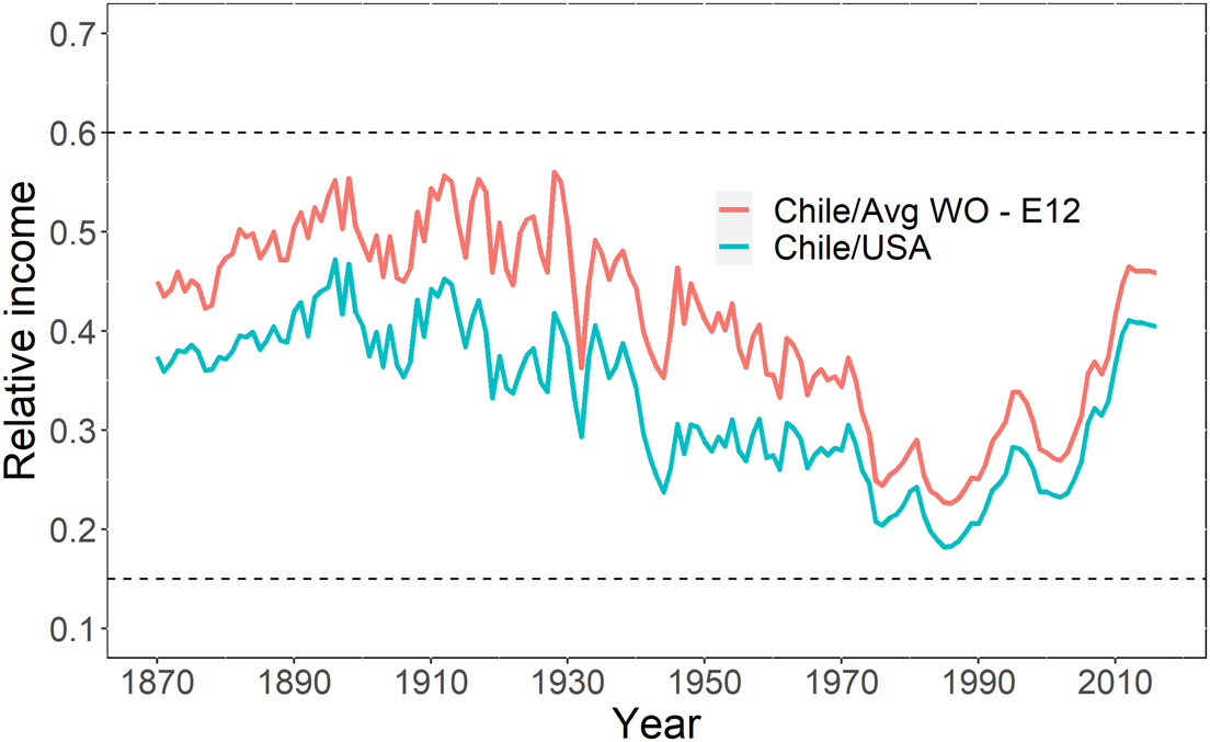
According to Im and Rosenblatt (Reference Im and Rosenblatt2013), a middle-income country is one that has an income per capita ranging from 15 to 60 per cent of U.S. income per capita. As a starting point, we follow the same definition and consider the long-run evolution of Chile's relative GDP to discover when the country could be classified as a middle-income country. After reaching an income per capita representing 44.2 per cent of U.S. income per capita in 1910, per capita income dropped to 27.5 per cent in 1960 (Figure 1). Figure 1 is relevant because it indicates that, during the period under review, the relative development process of the Chilean economy came to a halt; note that this seems to be independent of whether we use the United States as a benchmark, as can be seen when we observe the behaviour of the relative GDP per capita of Chile with respect to an average of Maddison's Western Offshoots and other Western European countries.
Relative income per capita.
Source: Maddison (2018).
Note: The horizontal lines represent the middle-income band. The line above shows the relative income between Chile and the average between Western Offshoots and Western Europe, while the line below shows Chile's relative income to the United States. Western offshoots is the average income of the United States, Canada, Australia and New Zealand together, while Western Europe is the average income of the group of countries comprised of: Austria, Belgium, Denmark, Finland, France, Germany, Center-North Italy, the Netherlands, Norway, Sweden, Switzerland and Great Britain.
Looking for evidence of the middle-income trap phenomenon, Eichengreen et al. (Reference Eichengreen, Park and Shin2014) identified growth slowdown episodes, defining them as such if they satisfied the following conditionsFootnote 4:
 $$g_{t, t-n}{\rm \;} \ge 0.035$$
 $$g_{t, t-n}-g_{t, t + n}{\rm \;} \ge 0.02$$
where y t is the actual gross domestic product per capita, g t,t−n and g t,t+n are the average growth rates between years t and t − n and between years t and t + n, respectively. The authors follow Hausmann et al. (Reference Hausmann, Pritchett and Rodrik2005) and, offering no other explanation, set n = 7Footnote 5.
As we study the long-run development process of Chile, we find that growth slowdowns occurred in 5 years/periods between 1820 and 1960. These were 1881–1884, 1910, 1912–1913, 1928–1929 and 1938–1940. Table 1 shows the growth rates before and after each of the Eichengreen-like deceleration episodes. The third column shows the gap between growth levels as estimated by the left side of (2), which satisfies the slowdown condition and ranges from 2.50 to 9.08 per cent.
Average annual growth rates, GDP per capita Chile.
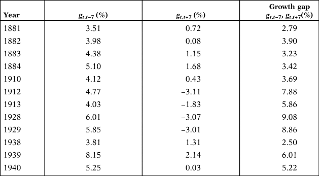
Source: Rgdpnapc variable from the Maddison Project Database (Reference Bolt, Inklaar, De Jong and Luiten Van Zanden2018).
From the 1920s, deceleration episodes became more intense, with an increasing difference between the g t,t−7 and g t,t+7 growth rates. This brought about greater divergence with respect to U.S. income per capita, reaching levels below 35 per cent by the time the last slowdown took place in 1940, after which Chile's relative income increasingly fell.
These growth slowdowns show that Chile experienced an economic decline that happened in line with Eichengreen et al. (Reference Eichengreen, Park and Shin2014)-type episodes for middle-income countries. Slowdowns also occurred during the Great Depression, which correlates with authors who claim the long-term decline of Chile started near that time (Fuentes Reference Fuentes2011; Haindl Reference Haindl2006). However, the analysis shown in the following sections demonstrates that the most significant decline started later.
4. STRUCTURAL BREAKS?
Any time series can be tested for structural breaks by using formal statistical tests. In our case, we are interested in knowing whether the time series of relative income for Chile has a structural break in the long run, for which we test the null hypothesis of no structural change in order to find out when we would be more likely to reject it. We implement an extended Chow test (Chow Reference Chow1960), as the Chow test has the disadvantage that we need to determine, in advance, the potential break date. Since, as we will examine below, several significant events had been taking place in Chile since the mid-1920s, and we do not know a priori when the potential break dates are, we perform the analysis on a year-by-year basis, estimating a series of F-statistics as in Zeileis et al. (Reference Zeileis, Leisch, Hornik and Kleiber2002), assuming the relative income series are constant. In this way, we compare two different models each year and compute the relevant test. The year the value is highest is the most likely structural break date.
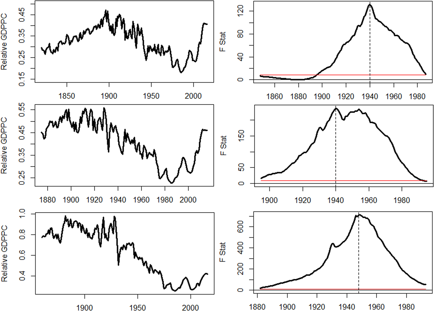
Figure 2 shows the results of year-by-year statistical structural change tests for the long term for three cases: the relative income per capita series between Chile and the United States; the one between Chile and the simple average of Maddison's Western Offshoots and Western Europe-12; and that between the relative income of Chile and the Nordic-3. The evidence here suggests that the most likely structural break date occurs in 1940 in the first two cases and in 1948 in the third.
Relative income and structural change: Chile/United States, Chile/Western Offshoots and Western Europe. Chile/Nordic-3.
Sources: see text.
Note: The top left figure shows Chile's GDP per capita relative to the United States, the middle left shows Chile relative to the simple average of Western Offshoots and Western Europe-12, and the bottom left one shows Chile's relative to the Nordic-3 countries. The figures on the right show the results of the F-statistic to test for a structural break in level as in Zeileis et al. (Reference Zeileis, Leisch, Hornik and Kleiber2002) for each series, assuming relative income is constant. The highest value marks the most likely year for structural break on the series. In this case, 1948 in the bottom case (Nordic-3), while 1940 in the other two. The period considered in the analysis changes as some European countries' data start later in the database.
For robustness, we performed Bai–Perron tests on the relative income series between Chile and the United States, and between Chile and the Nordic-3 countries, which seek to determine the years of optimal breaks in the series (Bai and Perron Reference Bai and Perron1998). Regarding the first series (Table 2), we find the most significant break in 1940, and find 1940 to be a break date independently of the number of structural breaks identified. Regarding the relative income series between Chile and Nordic-3 (Table 3), the optimal break year occurs in 1948 when we consider one break dateFootnote 6.
Break date from Bai–Perron's test: Chile–United States.
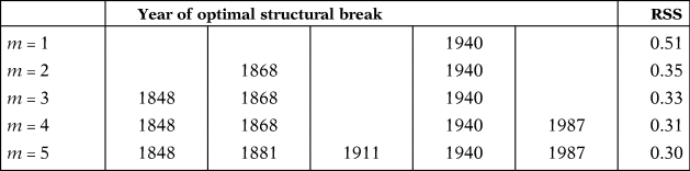
Note: The years show the optimal break dates according to the Bai–Perron test applied to the relative income per capita between Chile and the United States. The value of m indicates the number of breaks, while the RSS shows the residual sum of squares of the model. Data from Maddison Project Database (Reference Bolt, Inklaar, De Jong and Luiten Van Zanden2018).
Break date from Bai–Perron's test: Chile–Nordic 3.
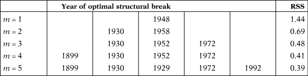
Note: The years show the optimal break dates according to the Bai–Perron test applied to the relative income per capita between Chile and the average of the Nordic 3 (Sweden, Norway, Finland). The value of m indicates the number of breaks, while the RSS shows the residual sum of squares of the model. Data from Maddison Project Database (Reference Bolt, Inklaar, De Jong and Luiten Van Zanden2018).
5. AND CHILEAN ECONOMIC HISTORY? A NARRATIVE
The «Parliamentary Period» in Chile, stretching from the aftermath of the War of the Pacific (1879-1883) to the 1920s, was characterised by the economic prosperity generated by the newly acquired nitrate deposits in Tarapacá and AntofagastaFootnote 7. The natural resource boom, firstly in nitrates, and beginning in the early 20th century in copper, generated significant linkages in the Chilean economy, although it did not generate an overall modernisation of the economy (Badia-Miró and Díaz Reference Badia-Miró, Díaz-Bahamonde and Kuntz-Ficker2017). Instead, inflation and political instability were persistent features of this period and were related to a gradual deterioration of macroeconomic management. Political instability led to macroeconomic instability, which was reflected in the fact that, between 1891 and 1924, the country had more than 90 ministers of finance (from evidence presented by Bernedo et al. Reference Bernedo, Camus and Couyoumdjian2014). In a broader sense, the struggle for the capture of the natural resource rents was a serious economic and political problem (Blakemore Reference Blakemore and Bethell1993).
Prosperity also brought about important social change, as well as increasing (or increasingly visible) inequality. This represented the coming of the so-called «social question» in Chile, with a related sense of national decline (Morris Reference Morris, H. and Godoy1971; Gazmuri Reference Gazmuri2001). In part, this decline was considered a failure of the national elites (Collier and Sater Reference Collier and Sater1996, p. 185). Despite the economic growth achieved during the 19th century, Chile had not attained an equivalent progress in social terms. For example, health progress was slow and the sanitary situation was very poor, transforming the country, as noted by a physician, into a «large hospital» (Sagredo Reference Sagredo2014, p. 172). Something similar happened with education. As Sagredo explained,
«Despite the progress made, at the beginning of the 1930s there was a critical view of the so-called Estado Docente, i.e., the public educational system implemented during the Republic. This was mainly because, with all its virtues, it was a highly unequal system providing quality education to urban elites, which did not pay for the privilege they received, but rather it was the entire population that paid the cost through taxes» (2014, p. 222).
Regarding the diffusion of public education, the slow progress (at least till the 1920s) was examined by Egaña (Reference Egaña2000), who noted the lack of conviction of the Chilean political class. From a comparative perspective, Ranestad (Reference Ranestad2018) considered the national deficits in this sense in terms of what she labelled a «knowledge gap» (with respect to Norway)Footnote 8.
The difficult social situation was compounded at the end of World War I. The role of this conflict is important in several dimensions here; during the war, Chile suffered a very significant fall in its imports, and in its aftermath, the nitrate industry suffered a significant shock as a result of the competition from synthetic nitrates (Couyoumdjian Reference Couyoumdjian1986; Albert Reference Albert1988). The first effect had a significant impact on the evolution of investment, specifically in physical capital formation in machinery. While this variable had increased significantly during the late 19th century, it was severely affected by the war and, later, by the Great Depression. Moreover, this type of investment exhibited a highly volatile behaviour, which led to an additional cost on overall economic activity (Hofman and Ducoing Reference Hofman, Ducoing, Yánez and Carreras2012; Ducoing Reference Ducoing2016).
The 1929 global crisis led to the collapse of the nitrate industry, and also affected the up-and-coming copper industry, producing a worsening of the country's social problems. The main problem was that tax revenues generated by the nitrate industry had been increasingly used to increase spending and reduce taxes, weakening the nation's public finances (Blakemore Reference Blakemore and Bethell1993). In other words, the Chilean state was suffering an important problem in terms of its fiscal capacity. This affected its capacity to provide public goods, especially in health and education, as noted above.
Undoubtedly, these factors contributed to the climate of social upheaval that eventually led to significant political instability (including political revolutions in 1924 and 1932). Collier and Sater (Reference Collier and Sater1996) asked «what had happened to the ‘model republic’?» (p. 188), and one cannot but agree with Harold Blakemore, who argued that «parliamentary leaders stand condemned … in their apparent inability not so much to recognize a society in transition, for most were aware of changes taking place, but to reform their institutions so as to cater to them» (Blakemore Reference Blakemore and Bethell1993, p. 67).
While the election of Arturo Alessandri in 1920 represented a reformist impulse, political instability continued and the president was ousted in 1924Footnote 9. Indeed, the period from Alessandri to Ibáñez has been labelled by Mario Góngora (Reference Góngora1981), as «el tiempo de los caudillos» («the time of the caudillos»), in a period marked by the increasing influence of the ideas of nationalism and the principle of social protection. Significant institutional reforms were passed in this era, including a new Constitution in 1925, and important pieces of social legislation approved in 1924, as well as the establishment of different development banks, including the Caja de Crédito Agrario (1926), the Caja de Crédito Minero (1927) and the Instituto de Crédito Industrial (1928). The formation of a «modern state» was an important ambition of Carlos Ibáñez; this new structure would be in charge of managing the problem of economic development in the ensuing decades (Ibáñez Reference Ibáñez2003).
When the 1929 crisis came, the Chilean economy was in a highly vulnerable position, still highly dependent on its export sector and with a very significant external debt. As a result, there were major economic, social and political consequencesFootnote 10. The political instability even led to the establishment of a short-lived revolutionary «Socialist Republic» in 1932, which naturally generated great uncertainty, and also saw the birth of long-lasting interventionist institutions, such as the Comisariato de Subsistencias y Precios (Commissariat of Subsistence and Prices) (Brahm Reference Brahm1999). In the medium term, the 1929 crisis deepened nationalist views and reinforced an increasingly influential belief regarding the importance of promoting industrial development, in a process that turned out to have clear corporatist elements. Here we find the foundations of a process of state-led and financed industrialisation that would represent an important transformation in the country. In this sense, Ellsworth (Reference Ellsworth1945) referred to the Chilean economy in the period after the Great Depression, as «an economy in transition».
Created in 1939, CORFO is thus the culmination of a gradual process during which there was a change in the prevailing ideas regarding the state's role in the economy. In a sense, the national context after the Great Depression and the major earthquake the country suffered in 1939 represented the perfect catalysts for the institutionalisation of these ideas. It should then be no surprise that the country's main economic and social actors participated in this process. As Muñoz and Arriagada (Reference Muñoz Gomá and Arriagada1977, p. 52) noted, industrialisation was a «political project», one which a new technocratic class also supported (Ibáñez Reference Ibáñez2003). It was up to the government of the Frente Popular, elected in 1938, to make this come about. This new administration was set on stimulating the process of economic development, and strongly endorsed,
«functions that no state agency had ever had before, such as the formulation of a national productive plan and the associated allocation of investment resources. This implied, on the one hand, that the state was assigned a function as coordinator of the interests of the different productive sectors, and on the other hand, a clear entrepreneurial function by being allowed to make direct public investments in activities different from traditional infrastructure projects» (Muñoz and Arriagada Reference Muñoz Gomá and Arriagada1977, p. 27.).
Even though the project finally approved involved a broad political negotiation in Congress (Ortega et al. Reference Ortega1989), the main elements of a symbiotic relationship between the state and the private sector (and including labour) were established here. It is in this context, with low levels of human capital, high inequality and social conflict, and extensive rent-seeking, that the country faced the World War II.
6. A SYNTHETIC CONTROL METHOD ANALYSIS
The SCM developed by Abadie and Gardeazabal (Reference Abadie and Gardeazabal2003) (see also Abadie et al. Reference Abadie, Diamond and Hainmueller2010, Reference Abadie, Diamond and Hainmueller2015) allows researchers to assess the effect of an intervention in a single treated unit (city, region, country, etc.) by making a synthetic control from a donor pool, which is a group of untreated units. This is useful in many cases where a unit by itself might not be an effective control because of its differences with the treated unit.
Our objective when using the SCM is twofold. First, we seek to formally determine when the Chilean economy started diverging from high-income nations. We constructed synthetic controls for Chile on a year-by-year basis and determined the root mean square prediction error (RMSPE) ratio for before and after the treatment. This analysis enabled us to discover which year shows the greatest divergence of Chile from its synthetic control, that is, we were able to determine when it is most likely that the country started diverging from the donor pool. Our second objective is to quantify what would have happened if the policies implemented beginning in 1939 had not been put into place.
The method consists in determining a vector of weights from the control countries, which together form a combination that represents (in our case) the counterfactual Chile that was not affected by the treatment. To determine the optimal vector of weights, a constrained optimisation problem must be solved in order to minimise the distance in the outcome variable between the treated unit and the synthetic control. Formally, to construct the synthetic control, assuming we observe a panel of J + 1 countries during T periods of time, and only one country receives the intervention in some T 0 < T, which stays in place until T, the effect of the treatment for country i in period t can be defined as:
 $${\rm \;\;}\tau _{it} = Y_{it}^I -Y_{it}^N $$
where  $Y_{it}^I $ is the observed value of the outcome variable (in our case gross domestic product per capita), while $Y_{it}^N $ is the value if the intervention had never taken place. Let i = 0 be the country affected by the treatment. It follows that $Y_{0t}^I = Y_{0t}^{{\rm obs}} $, where $Y_{0t}^{{\rm obs}} $ is the observed value of the outcome variable, and that $\tau _{0t} = Y_{0t}^I -Y_{0t}^N $, with the value of $Y_{0t}^N $ being unobserved.
Note that we assume the treatment has no effect before its implementation, in other words,  $Y_{it}^I = Y_{it}^N $ for every t < T 0. In the case of having anticipation effects, we could simply redefine T 0 as some other t < T 0.
The SCM determines an estimator of  $Y_{it}^N $ with the following linear structure:
 $$Y_{it}^N = \mathop \sum \limits_{i = 1}^J w_iY_{it}^{{\rm obs}} $$
 The value of the outcome variable,  $Y_{{\rm it}}^N $, is a linear combination of the control countries, with weight w i for country i. Weights are required to be positive and add up to one.
For estimating the parameters, let Y 1 be a vector of T 0x1 values of the outcome variable for the treated country, and let Y 0 be a matrix of T 0xJ with the same variable for each of the J countries in the donor pool. The weights on the model are chosen so that the distance between the outcome variable of the synthetic control and the treated unit is minimised. The optimisation problem can be expressed as:
 $$W^{\rm \ast } = {\rm argmi}{\rm n}_w( {Y_1-Y_0W} ) ^{\rm ^{\prime}}( {Y_1-Y_0W} ) $$
The weights can also be estimated by minimizing the distance between a set of covariates, as in Abadie and Gardeazabal (Reference Abadie and Gardeazabal2003) and Abadie et al. (Reference Abadie, Diamond and Hainmueller2010). However, due to the lack of data about relevant covariates as investment levels and shares of gross domestic product, only data on the outcome variable are used.
A limitation of the SCM is that it does not permit accounting for the significance of the results using standard inferential techniques, as these methods rely on large randomised samples and several treated units. The SCM requires a relatively small sample and a single treated unit, and because it provides a systematic way to choose comparison units, placebo tests can be used to make a quantitative inference. This consists of applying the SCM to every country in the donor pool and comparing the values of the outcome variable between each one and its synthetic counterpart.
In a country panel setup, for the synthetic control to represent the behaviour of a country in a variable of interest after the treatment starts, it should also resemble the country's behaviour in the periods before the treatment. Several articles utilise the SCM for studying the impact of policy changes and other exogenous events in comparative case studies; it has been applied in different contexts in the social sciences, from estimating the impact of terrorism on long-term growth (Abadie and Gardeazabal Reference Abadie and Gardeazabal2003), to estimating the effects of political figures such as Hugo Chavez in Venezuela (Grier and Maynard Reference Grier and Maynard2016), to the «rise and fall» of the Argentinean economy (Spruk Reference Spruk2019) and the economic impacts of natural disasters (Lynham et al. Reference Lynham, Noy and Page2017).
The implementation of the method is carried out in Matlab and consists in solving the optimisation problem given in equation (5) with the Maddison project database (2018) GDP per capita data for the countries previously chosenFootnote 11. To construct our synthetic controls, we used a control group of countries that did not implement similar policies nor had the same shocks. We consider first the countries that have data during the period under study (1900–1960) and without any gaps. When we consider the requirement for control countries, that is, that they are not affected by similar treatments as the unit under study, we exclude other Latin American countries; after all, all of them applied strong restrictions on trade during the period under study (Edwards Reference Edwards2009). We also opted to exclude countries that had high levels of involvement in World War II as it is an unrelated profound structural shock in the economyFootnote 12, and we exclude Asian countries given their larger difference from the Chilean economy in comparison to western countries. The next consideration is to keep countries that are relatively like the treated unit in GDP covariates. We thus end up with the following control group of nine countries: Australia, Canada, Switzerland, Denmark, Finland, Norway, New Zealand, Sweden and Portugal.
As noted, there are several possible events/dates that could have triggered the changes we are examining in Chile. We performed a synthetic control for every year t between 1924 and 1950, for which we took annual data on GDP per capita (from Angus Maddison's database) between 1900 and t–1 for each case.
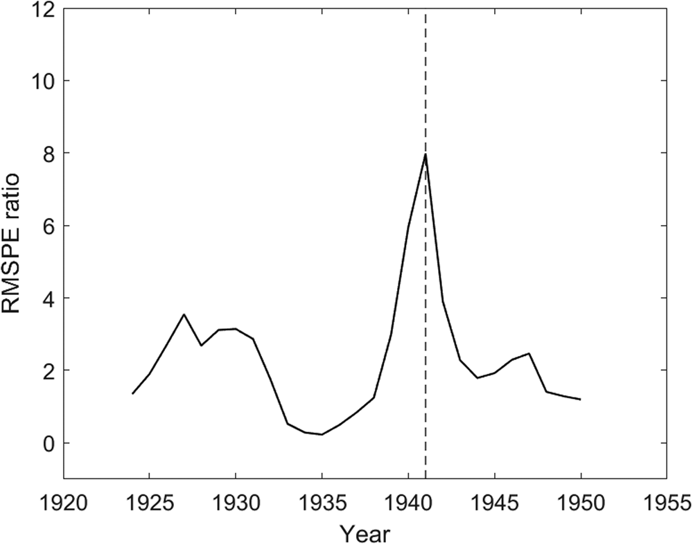
Figure 3 presents a plot of the ratio between post-treatment RMSPE and pre-treatment RMSPE against the chosen treatment year. For consistency, an interval of 5 years before and after treatment is considered when calculating the RMSPEs. As noted above, due to data availability, in this work we only consider the income (GDP) per capita series without modelling the determinants of GDP; this is an exercise that will remain pending for the future. The results show that the likelihood of a shock is highest in 1941. This result is consistent with that of the previous section and indicates a break point for a year that more or less coincides with the first National Accounts estimates for Chilean GDP (1940). This highlights the quality of the data we are working with, which is an unavoidable constraint, for our analysisFootnote 13. Indeed, the history of the system of National Accounts around the world is an effort at establishing international standards, and one of the continual methodological innovationsFootnote 14. At any rate, we cannot be sure whether the measurement error we face is what drives our results; a better measure of GDP could correct previous biases in any direction.
RMSPE (Root Mean Square Prediction Error)-ratio.
Note: Ratio of the post-treatment RMSPE to the pre-treatment RMSPE between Chile and its synthetic counterfactual estimated changing the start of treatment from 1925 to 1950. An interval of 5 years from and after the treatment is considered when calculating the error term.
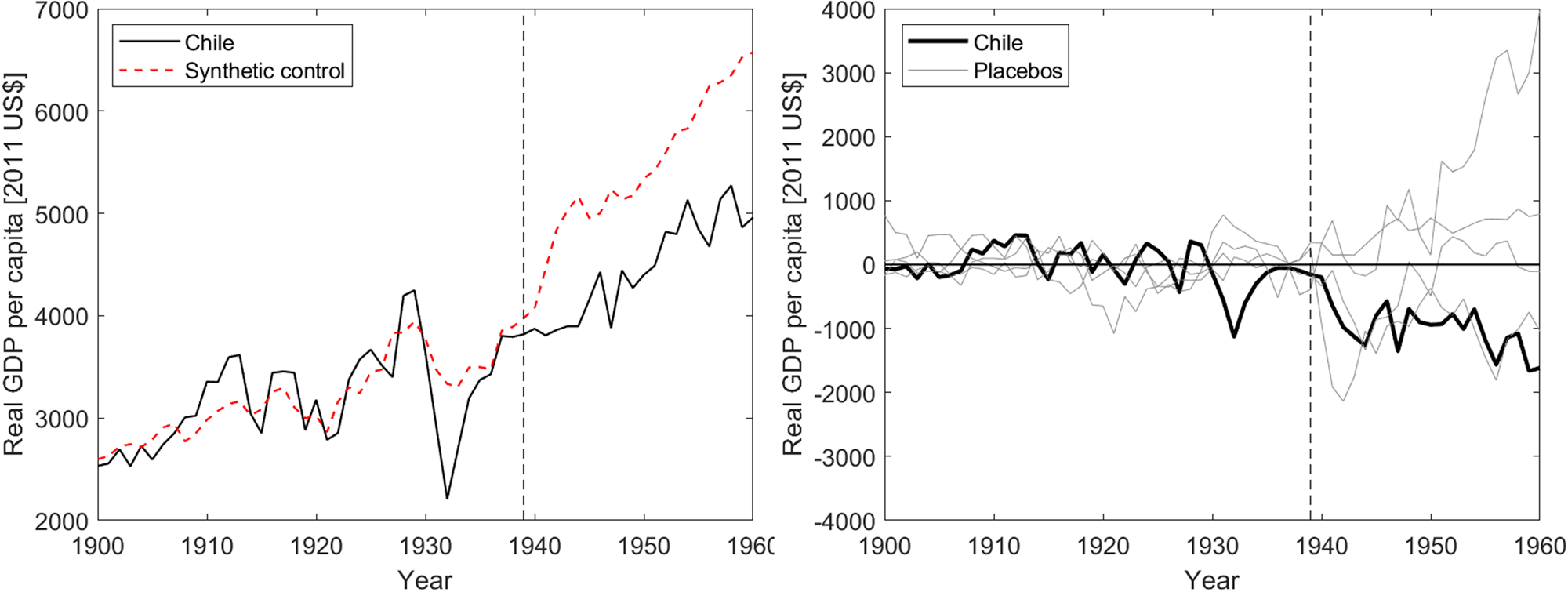
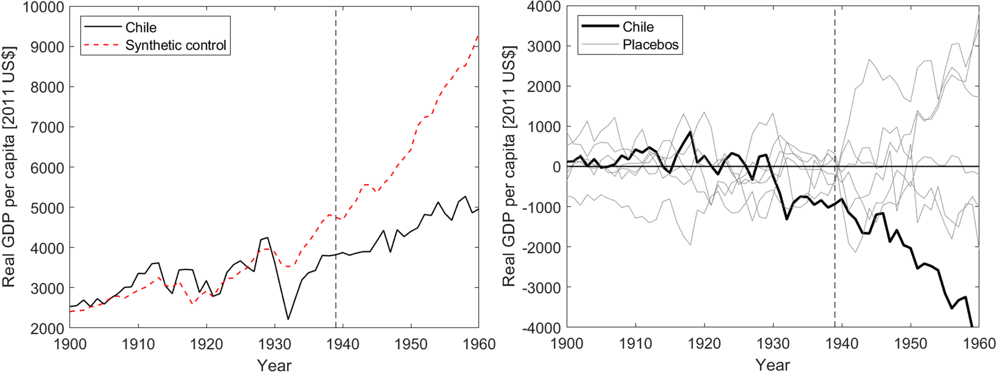
Next, we show the result of our main synthetic control, which follows the discussion in the previous section, setting 1939 as the year when the treatment beginsFootnote 15. When resolving the optimisation problem, we obtained a synthetic unit composed of a weight of 23.5 per cent Canada, 4.5 per cent New Zealand and 72.0 per cent Portugal (see Table 4). Figure 4 shows Chile's income per capita and its synthetic control for the entire period under consideration, along with the placebo robustness test. As seen, the synthetic control echoes the path followed by Chile very accurately until 1939, replicating the economic cycles in the previous decades. When the treatment begins, an instant and dramatic effect is observed on the income per capita level. Only 5 years after 1939, the gap is US$1,268 per capita, which is equivalent to 32.3 per cent of Chile's income level that year. Moreover, this difference is persistent over time. The placebo test shows that only one other country presents a larger negative gap after treatment, and only momentarily. This makes us confident that the synthetic control is identifying a unique treatment for Chile that had a significant effect on income.
Synthetic control and placebo test.
Note: The synthetic control for Chile with the treatment set in 1939 is shown on the left side. The solid line shows Chile's GDP per capita from Maddison's data: Bolt et al. (Reference Bolt, Inklaar, De Jong and Van Zanden2018). The dashed line shows the synthetic control constructed from the control group. A placebo test is shown on the right side, where the black line represents Chile's GDP per capita gap with its synthetic control, and the lighter lines show the gap for the other countries in the sample with each country's own synthetic control. Only countries with a pre-treatment RMSPE of less than 1.5 times that of Chile are shown.
Country weights from SCM.

Sources: See text.
The RMSPE for the pre-treatment period is US$314.8, indicating that the average of the square root of the squared errors between Chile and its synthetic control corresponds to US$314.8 before 1939. After the treatment, the value of the RMSPE is US$1,043.2, with a 3.31 ratio between post and pre-treatment RMSPEs.
6.1 A Jackknife
As an additional robustness test, we repeated the exercise while removing Portugal from the sample due to its larger weight. The results are shown in Figure 5. As seen, the results are not sensitive to the exclusion of Portugal, and the placebo holds with Chile showing the greatest negative gap over the entire post-treatment period. The optimal weights for this case are: 13.7 per cent Canada, 75.8 per cent Finland and 10.6 per cent Norway. The pre-treatment RMSPE is US$493 and the post-treatment US$2,442.
Jackknife test and placebo.
Note: Same as in Figure 4, with the highest weighted country left out of the sample as a robustness test. In our case, this country is Portugal.
7. DISCUSSION: BACK TO HISTORY
The results in the previous section point to a new date for the relative divergence of the Chilean economy. Together with the historical narrative presented in section 5, this suggests that in terms of the economic history of Chile, the period between the end of the World War I and the start of the World War II merits careful examination. The factors that the literature identifies as the main determinants of the middle-income trap: low levels of human capital—and, more generally, a weak state capacity—, high inequality, social conflict, and social and political unrest, are all present in the period we examine. Other exogenous shocks, such as pandemics (including smallpox and cholera) and earthquakes, were also present. In this section, we return to our reading of the history of Chile, now under these lenses; this will mean elaborating on some points examined in section 5, and further discussing the historical evidence.
Following Góngora (Reference Góngora1981, p. 75), the renewed interest in confronting the «social question» in 1920s Chile could actually be labelled a rediscovery. For some time, different political sectors had been proposing policies to address this problem, which was a consequence of emerging urbanisation and industrialisation; the increasing consciousness of a new «working class», which includes workers in the nitrate sector, is also relevant here. It should be no surprise to observe that this was accompanied with increasing social unrest, as can be seen in different strikes, public demonstrations and clashes with the police during this decade (although this is also part of a process that had been going on for the last few decades; indeed, a national strike, in 1919, ended in the imposition of a state of siege in the country). Reflecting a decline in the tradition of classical economics and a stronger influence of social democratic parties, the responses adopted during this decade resulted in new social legislation and a greater government intervention in the economy.
The downfall of the nitrate industry during the 1920s had important fiscal effects, specifically in terms of weakening national public finances. This weak fiscal capacity affected the government's capacity to provide public goods, thus representing a larger problem of state capacityFootnote 16. These new problems evidence how, during the nitrate era, the fiscal dependence on export taxes and the related struggle for the capture of these rents represented a political version of the natural resource curse (Badia-Miró et al. Reference Badia-Miró, Pinilla and Willebald2015). Apart from the issue of the larger or smaller vertical linkages generated throughout the economy during this period and of the existence or extent of a «Dutch disease», an important part of this problem was related to rent-seeking and a type of state capture, plus a related lingering feeling that the country squandered its riches which deepened the ideological changes and social fractures referred to above (Blakemore Reference Blakemore and Bethell1993).
After the political instability of the mid-1920s, the new Constitution dealt with the political problems, and at the same time a new administrative state gathered force. The Kemmerer reforms and the efforts by Carlos Ibáñez and his minister of finance, Pablo Ramírez, to reorganise the public administration, including the fiscal system, were an attempt to address the fiscal (and inflationary) problems. However, the «modern state» that was emerging became an arbiter of the interests of different groups in a process that epitomised the consolidation of corporatist ideals (Ibáñez Reference Ibáñez2003); to note one specific example in this sense, consider the creation of a Consejo de Economía Nacional (National Economic Council) formed in 1932, and resurrected in 1934 with the backing of the country's main business associations. The nationalism implicit in this program can be gathered by the accompanying escalation in protectionist trade policies, which had been gaining ground since the late 19th century. Together with the activities of the newly instituted development banks (the Cajas referred to above), this signalled a major shift in the country's economic policies (Góngora, Reference Góngora1981).
As a result of the Great Depression, the Chilean economy (and political system) were strongly affected but the administrative state remained strong; as an example, note that protectionist policies acquired a new face, and a new scale. Specifically, Lüders and Wagner (Reference Lüders and Wagner2003) have stressed the role of exchange rate management as another (new) instrument for protectionist policies. This was possible once the monetary discipline associated with the gold standard was abandoned, and in the ensuing years, exchange rate policy turned out to be a complex and highly discriminatory system, as Baerresen (Reference Baerresen1969) has shown. One would expect that the costs of such policies in terms of the allocation of resources would be significant and accumulative.
As noted, the development and stimulus of an industrial sector, led by the state, was an important motivation of the CORFO. Actually, different actors were part of the political impulse that led to the formulation of an explicit national industrialisation plan, including a technocratic team of engineers who would eventually be in charge of CORFO (Muñoz and Arriagada Reference Muñoz Gomá and Arriagada1977); this explains the organisation of the agency's board, which included representatives of different business sectors and labour associations.
The development plans CORFO was directed to generate were not immediately introduced, and were postponed, presumably because of the earthquake, World War II, and a general lack of information regarding the productive structure of the Chilean economy. Thus, the agency's actions were organised around Planes de Acción Inmediata; this led to a significant industrial modernisation (Ortega et al. 1989, pp. 75–110), one which, however, was taking place in a context where, as noted, national industry would be highly protectedFootnote 17.
The middle-income trap framework is based on political and economic factors; implicitly here we find a crucial role for the political angle of the process of economic decline, which is also present in the literature on the political economy of development (e.g. Olson Reference Olson1982; Acemoglu and Robinson Reference Acemoglu and Robinson2006). Our narrative and analysis suggest that the main drivers of the divergence we study are related to the political nature and organisation of the state-led industrialisation process, with the related rent-seeking, and the misallocation of resources that was a consequence of the accompanying protectionism. Because of these constraints, this process did not realise its objectives. In this sense, part of our line of reasoning is related to the arguments advanced by Fajnzylber (Reference Fajnzylber1983), on the «truncated» industrialisation in Latin America; in comparison with East Asia, the industrial sector in Latin America was very dependent on protectionism and state subsidies, and unable to generate sustained increases in what we would now call total factor productivity. The lagged growth in the mining and agricultural sectors, the main export sectors of the Chilean economy, is another part of our argument (Ahumada Reference Ahumada1958); these were sectors that did not do as well in the redistributive political game of economic policy.
A related factor is the «regime uncertainty» (Higgs Reference Higgs1997) Chile began to experience in the mid-1920s, in a process related to ideological and political change; surely this affected private investment decisions and the allocation of resources in the economy. In terms of the evolution of economic policy, Bernedo, Camus and Couyoumdjian encapsulate the consequences of this institutional deterioration, institutional in the widest sense, in terms of the return of inflation, a recurring malaise of the Chilean economy after the World War II:
«Since the election of Pedro Aguirre Cerda [in 1938], a long-term, difficult to control inflationary process whose multiple causes are complex to isolate and define, was reactivated in our country. The funding of the industrialisation policy, foreign trade disruptions as a result of the Second World War, fiscal indebtedness, uncontrolled monetary issues, the growth of the state apparatus, and the pressures exerted by workers’ unions and associations to raise their remunerations are factors contributing to a rise in inflationary processes» (Bernedo et al. Reference Bernedo, Camus and Couyoumdjian2014, p. 113).
Repressed growth and inflation were both problems in Chile during the period of state-led industrialisation during the second half of the 20th century, a process which would eventually lead to a more generalised process of economic planning in the country.
8. CONCLUSIONS
In this paper, we have studied the problem of why countries suffer from growth slowdowns which lead them to diverge from developed countries. In this sense, we focus on the evolution of relative GDP which provides an accurate representation of long-run economic progress and decline, a process that involves international comparisons. Current literature believes that countries experiencing these slowdowns are suffering from the middle-income trap. We focused on the long-term economic history of Chile and different structural break tests showed that there was a significant change in Chile's relative income long-term time series in 1940, which is confirmed whether we are comparing with the United States or with an average formed by Maddison's Western Offshoots and Western Europe-12. While this coincides with the beginning of Chilean national accounts, we do not have any reason to believe that this is what is driving our results, and an analysis based on a comparison with a group of Nordic countries suggests that the process of divergence we are considering started sometime later, in 1948, which is also later than what conventional wisdom suggests.
We speculate that this was a process related to institutional (and ideological) changes. As we studied different aspects of the political economy of Chile in this period, we argue that the establishment of CORFO in 1939, which consolidated a new process of state-led industrialisation in the country that was related to the interplay of interest groups and nationalist and corporatist ideals, was a crucial eventFootnote 18. The political constraints within which this process took place, with a need to merge different interests which led to other distortions turned out to be an important problem. Although further work may be required to identify the precise causal mechanisms at play, our story is consistent with the political economy of economic development which focuses on rent-seeking and distributive games, as examined by, for example, Olson (Reference Olson1982), Acemoglu and Robinson (Reference Acemoglu and Robinson2006) and Mokyr (Reference Mokyr2016), who emphasises the role of ideology in this process.
While our analysis provides an explanation for the beginning of the divergence of the Chilean economy, the SCM exercise also represents a counterfactual analysis; this is, of course, one way in which hypotheses are tested in the social sciences. As Bunzl has explained, counterfactual reasoning plays an «unavoidable implicit role» in history (2004, p. 857). However, this type of analysis has sometimes been intended to be more than that. In contrast to the modern advocates of counterfactual history (e.g. Ferguson, Reference Ferguson1997), we do not wish counterfactual reasoning to be our main subject of interest (Bunzl Reference Bunzl2004), and we are aware of the criticisms on the misuses of such narratives (Evans Reference Evans2013). When engaging with Evans, Sunstein (Reference Sunstein2016) makes the point that problems with speculative and inconsistent counterfactual histories are one thing, but when historians attempt to explain the past they also deal with identifying the causes of what happened, and this involves some type of counterfactual. This is the way we interpret our analysis, and this is how we rationalise our inquiry into the middle-income trap and its causes.
In all, our results point to the importance of re-examining the conventional wisdom regarding the influence of the Great Depression on the relative economic decline experimented by Chile during most of the 20th century. The middle-income trap framework we have proposed presents lessons for countries suffering similar growth slowdowns in present times.
ACKNOWLEDGEMENTS
Under different titles, previous versions of this paper have been presented at WINIR 2017, SECHI 2017, Ridge Workshop on Economic History 2018 and seminars at the Universidad del Desarrollo. Comments from participants, especially Manuel Llorca-Jaña and José Díaz, are acknowledged. We are also grateful to John Londregan and, especially, to the referees and editors of this journal for their very helpful comments and suggestions. Of course, the usual caveat applies.



