


1. Introduction
Additive manufacturing (AM), and fused layer modelling (FLM) in particular, has found widespread adaption (Wohlers Reference Wohlers2017, Reference Wohlers2019). FLM is used to produce prototypes and parts with relatively inexpensive AM machines when compared to other AM processes. Like all other processes, it requires specific design guidelines to unleash its full potential: Design for Additive Manufacturing (DfAM), that is, a ‘set of methods and tools that help designers take into account the specificities of AM’ (Laverne et al. Reference Laverne, Segonds, Anwer and Le Coq2015). If such design measures are not implemented, design results may stay below their potential in design freedom, function integration, visual clues or sustainability, among others (Rosen Reference Rosen, Chua, Yeong, Tan and Liu2014; Thompson et al. Reference Thompson, Moroni, Vaneker, Fadel, Campbell, Gibson, Bernard, Schulz, Graf, Ahuja and Martina2016; Blösch-Paidosh & Shea Reference Blösch-Paidosh and Shea2019). Opportunistic DfAM methods try to exploit such potential. If guidelines are omitted, designs even might not be manufacturable, as restrictions of the AM process, materials or qualification are not considered properly. Such requirements are usually accounted for by restrictive methods (Laverne et al. Reference Laverne, Segonds, Anwer and Le Coq2015; Kumke Reference Kumke2018).
The FLM process (Figure 1a) allows for the layerwise production of free-form geometries by extrusion of continuous thermoplastic filament. These exhibit anisotropic behaviour even when using isotropic filament as a raw material (Ahn et al. Reference Ahn, Montero, Odell, Roundy and Wright2002), as parts are build up bead by bead (Figure 1b).
(a) FLM printing using a Raise3D Pro2 Plus printer. (b) Part build-up bead by bead using carbon fibre reinforced polymer filament.

For example, using nonreinforced acrylonitrile butadiene styrene (ABS) as raw material, yield strength was reduced by −44% (Rodríguez, Thomas & Renaud Reference Rodríguez, Thomas and Renaud2003) from longitudinal (beads aligned with load direction) to transverse direction (beads orthogonal to load direction in printer’s XY plane). Furthermore, (PLA) was printed on a Prusa i3 printer (Lanzotti et al. Reference Lanzotti, Grasso, Staiano and Martorelli2015) with orthogonal-to-longitudinal reduction in Young’s modulus of around −17%. As four longitudinal shell perimeters were used to print the specimen for both 0° and 90° infill patterns, actual reduction of Young’s modulus might be even larger when using only orthogonal infill patterns. Another scrutiny of strength reduction ranged from −86% (zero air gap) to −10% (0.0762-mm air gap, ABS on a Stratasys FDM 1650; Ahn et al. Reference Ahn, Montero, Odell, Roundy and Wright2002). It becomes obvious that results are largely dependent on process parameters, encompassing air gap (negative air gap means overlap between beads), road width, model temperature, layer height and similar. Longitudinal-to-transverse ratio of mechanical properties is called Degree of Orthotropy (DoO) in the following, further specified by DoO (E) for Young’s moduli and DoO (UTS) for tensile strength.
To improve mechanical properties of FLM parts, the use of fibre-reinforced plastics (FRP) filament has often been suggested and showed up to be effective (Parandoush & Lin Reference Parandoush and Lin2017; Blok et al. Reference Blok, Longana, Yu and Woods2018; Kabir, Mathur & Seyam Reference Kabir, Mathur and Seyam2020). These FRPs further increase anisotropy in FLM. Exemplary degrees of orthotropy for short FRP are given in Table 1.  $ {E}_{\parallel } $ is Young’s modulus in extrusion path direction, $ {E}_{\perp } $ is perpendicular Young’s modulus within printing plane, UTS is Ultimate Tensile Strength, accordingly, CF is carbon fibre and GF is glass fibre, all units in MPa. These values have been extracted from a recent research paper listing a variety of experimental studies on the mechanical behaviour of FLM-printed specimen in longitudinal and transverse directions (Brenken et al. Reference Brenken, Barocio, Favaloro, Kunc and Pipes2018).
Mechanical properties of FRP-FLM specimen in MPa, adapted from Brenken et al. (Reference Brenken, Barocio, Favaloro, Kunc and Pipes2018).  $ {E}_{\parallel } $: Young’s modulus in extrusion path direction; $ {E}_{\perp } $: perpendicular; $ {UTS}_{\parallel, \perp } $: Ultimate Tensile Strength, accordingly; all beforementioned in MPa. DoO: degree of orthotropy, ratio of longitudinal-to-orthogonal Young’s modulus in printing plane $ E $ (stiffness) and $ UTS $ (strength). CF: carbon fibre; GF: glass fibre.
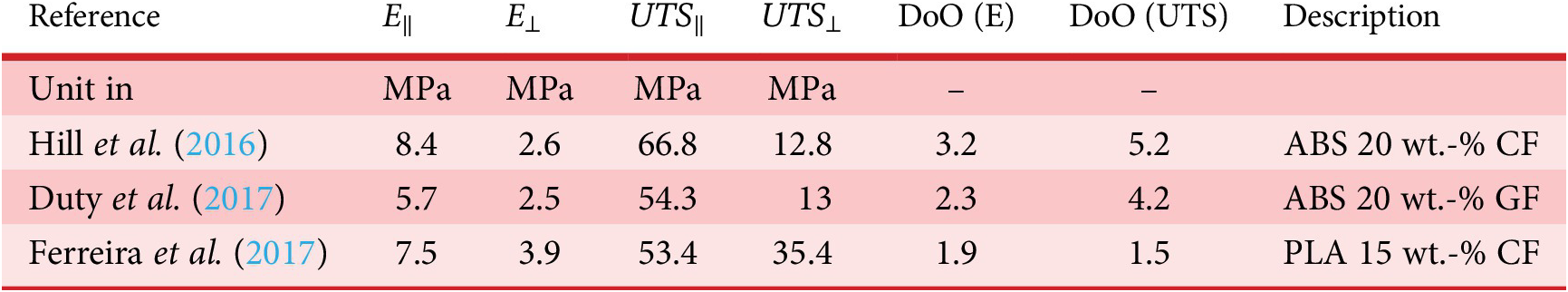
In the z-direction perpendicular to the build platform, between layers, Love et al. (Reference Love, Kunc, Rios, Duty, Elliott, Post, Smith and Blue2014) even found a DoO of 5.9 in stiffness and 10.1 in strength with 13 wt.-% CF. Thus, it must be stated that taking anisotropy into account during the design stage for FRP-FLM parts is crucial to obtain mechanical behaviour that meets all requirements. This is only partly reflected in current optimization approaches. These target specific FLM optimization problems (Brackett, Ashcroft & Hague Reference Brackett, Ashcroft and Hague2011; Liu et al. Reference Liu, Gaynor, Chen, Kang, Suresh, Takezawa, Li, Kato, Tang, Wang, Cheng, Liang and To2018; Fu et al. Reference Fu, Huang and Liu2019). Dapogny et al. (Reference Dapogny, Estevez, Faure and Michailidis2019) derived geometry which is dependent on chosen infill raster. A topology optimization (TO) method for transversally isotropic materials for stiffness was proposed by Nomura et al. (Reference Nomura, Dede, Matsumori, Kawamoto, Li, Steven and Zhang2015b) and Liu et al. (Reference Liu, Gaynor, Chen, Kang, Suresh, Takezawa, Li, Kato, Tang, Wang, Cheng, Liang and To2018). A TO method for consideration of strength was proposed by Mirzendehdel, Rankouhi & Suresh (Reference Mirzendehdel, Rankouhi and Suresh2018). Metamodel-based build orientation optimization was introduced (Ulu et al. Reference Ulu, Korkmaz, Yay, Burak Ozdoganlar and Burak Kara2015). Villalpando, Eiliat & Urbanic (Reference Villalpando, Eiliat and Urbanic2014) researched structure optimization on various parameters. Furthermore, FLM optimization less targeted on anisotropy was explored such as support structure optimization (Garaigordobil et al. Reference Garaigordobil, Ansola, Santamaría and Fernández de Bustos2018; Kuo et al. Reference Kuo, Cheng, Lin and San2018; Pellens et al. Reference Pellens, Lombaert, Lazarov and Schevenels2019; Thore et al. Reference Thore, Grundström, Torstenfelt and Klarbring2019) and optimization for build time reduction (Sabiston & Kim Reference Sabiston and Kim2020).
2. Motivation and objective
However, recent approaches still have some shortcomings besides their capabilities. In Brackett, Ashcroft & Hague (Reference Brackett, Ashcroft and Hague2011), general issues and opportunities for the application of TO are reported. Issues relate to mesh resolution (very fine mesh is necessary to depict AM-producible details) and lack of manufacturing constraints (like overhang constraint to avoid support structures). The usage of lattice structures in TO, which account for intermediate density (‘grey’) areas, multimaterial design, and process parameter variation are considered as DfAM opportunities to improve structural behaviour. The approach proposed in the contribution includes a modification of a bidirectional evolutionary structural optimization (BESO) method to consider overhang constraints. A generic workflow is outlined for AM-TO without detailing steps such as subsequent redesign. The approach in Liu & To (Reference Liu and To2017) is more comprehensive and includes build direction optimization and material anisotropy using a Level-Set structural optimization method. Isovalue level-set contours are chosen as printing paths, and the so-induced anisotropy is considered by the Level-Set TO algorithm. Like this, the TO result is dependent on inner extrusion paths. On the upside, paths run very smoothly and thus are suitable for manufacturing requirements. However, extrusion paths are not originally optimized for a specific mechanical objective like maximum stiffness or strength. From an efficiency perspective, the authors state an efficiency gain when compared to former Level-Set-based optimization methods: Their algorithm needs 150 iterations for a cantilever fixed-geometry problem and more iterations when geometry is not fixed. There is no comparison to BESO or mathematical TO algorithms. In Dapogny et al. (Reference Dapogny, Estevez, Faure and Michailidis2019), different ‘crust-and-bulk’ (shell and infill) models of FLM parts are analysed for their mechanical properties and optimization is conducted using different infills, again not directly modifying the infill concurrently with the outer shape. Build orientation optimization is not conducted, as only 2D geometries are scrutinized. TO using isoparametric projection is conducted in Nomura et al. (Reference Nomura, Dede, Lee, Yamasaki, Matsumori, Kawamoto and Kikuchi2015a, Reference Nomura, Dede, Matsumori, Kawamoto, Li, Steven and Zhang2015b), which is suitable to derive macrogeometry and innermaterial orientation simultaneously. Proof is also given that such an approach is effective; however, there is no further application on FLM or AM specifically. Following up, Zhou, Nomura & Saitou (Reference Zhou, Nomura and Saitou2019) present an extensive AM-TO method for assemblies including build orientation and material behaviour, and optimization at joints and maximum stress constraints is presented. This approach does, however, not consider detailed within-layer orientation. Mirzendehdel, Rankouhi & Suresh (Reference Mirzendehdel, Rankouhi and Suresh2017, Reference Mirzendehdel, Rankouhi and Suresh2018) present a TO method considering anisotropy and failure criteria (Tsai-Wu) using a  $ \pm 45{}^{\circ} $ raster orientation within the part, stating that also more complex models can be used. Post-TO steps are not reported. Ulu et al. (Reference Ulu, Korkmaz, Yay, Burak Ozdoganlar and Burak Kara2015) explore build orientation under maximization of the factor of safety and extend this using surrogate models, but TO is not considered. Parametric internal structures of AM parts are optimized in Villalpando, Eiliat & Urbanic (Reference Villalpando, Eiliat and Urbanic2014), for example, requiring a macrogeometry beforehand. There are some approaches on extending TO algorithms for AM constraints, especially overhang (Garaigordobil et al. Reference Garaigordobil, Ansola, Santamaría and Fernández de Bustos2018; Thore et al. Reference Thore, Grundström, Torstenfelt and Klarbring2019), minimum length and overhang (Pellens et al. Reference Pellens, Lombaert, Lazarov and Schevenels2019), support structure design within TO (Kuo et al. Reference Kuo, Cheng, Lin and San2018), build time reduction and support (Sabiston & Kim Reference Sabiston and Kim2020) or overhang and support (Gaynor & Guest Reference Gaynor and Guest2016). Concerning derivation of printing paths, many approaches focus on the production view (build time reduction, warpage minimization, support structure avoidance and similar; e.g., Yang et al. Reference Yang, Fuh, Loh and Wong2003; Wang, Xi & Jin Reference Wang, Xi and Jin2007; Hayasi & Asiabanpour Reference Hayasi and Asiabanpour2009; Brown & de Beer Reference Brown and de Beer2013; Jin, He & Fu Reference Jin, He and Fu2013; Alsoufi & El-Sayed Reference Alsoufi and El-Sayed2017; Coupek et al. Reference Coupek, Friedrich, Battran and Riedel2018; Mi, Wu & Zeng Reference Mi, Wu and Zeng2018; Volpato & Zanotto Reference Volpato and Zanotto2019). However, there is a lack of infill patterns design for mechanical properties optimization.
Overall, optimization of extrusion paths in individual layers is lacking in existing approaches. This is a promising way to improve mechanical properties of parts, as anisotropy is prevalent. Furthermore, existing approaches are limited in their comprehensiveness, as they do not cover the whole design process from boundary conditions and load to the final part, but rather some steps of it and mostly without interlinking. By linking build orientation, TO and proper orientation of extrusion paths, according to load paths, it seems possible that further lightweight potential can be exploited. To provide a basis for a comprehensive consideration of anisotropy for structural optimization of FLM parts in the following a structured, computer-aided engineering-based approach is presented.
3. Methods
The optimization approach consists of four steps: (1) load-path-dependent build orientation optimization; (2) TO considering orthotropic material properties; (3) derivation of printing paths and (4) simulation and printing. Proper printer z-axis alignment (layer build-up direction) to load path is important, as usually interlayer stiffness and strength are less strong compared to intralayer. Therefore, build orientation is done first before TO, which then uses projected material orientations within the determined layer planes (the XY plane of printer). This follows the rationale that if TO was used first, many TO runs would have to be conducted with different z-axis alignments, that is, projection planes for material orientations. Previous build orientation demands just one TO run. The order of the remaining steps (3) and (4) is straightforward, as printing paths are derived from TO, and simulation of FLM parts requires ready-to-print geometry with its extrusion paths’ orientations represented in building source (here: G-Code).
3.1. Load-path-dependent build orientation optimization
As laid out in the introduction, significant stiffness and strength reduction in transverse direction to the extrusion beads occurs. A particularly large reduction affects interlayer z-direction (Love et al. Reference Love, Kunc, Rios, Duty, Elliott, Post, Smith and Blue2014). Therefore, a load-path-dependent build orientation optimization seems promising to improve mechanical properties of a part. In this subsection, such an approach is presented.
To obtain a stiff and strong structure, load should be primarily transferred within the layers parallel to the build platform’s XY plane. Thus, load transfer through the weaker z-direction can be avoided. The principle of the build orientation optimization procedure is laid out in Figure 2.
Build orientation optimization approach using magnitude-weighted principal normal stress trajectories (PNSTs) for each load case (LC).
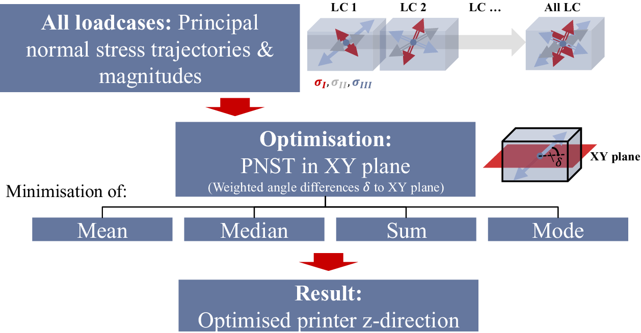
Step 1, load-path calculation, is conducted by calculating the principal normal stress trajectories (PNSTs) of a Finite-Element (FE) model under applied boundary and load conditions. The eigenvectors’ difference angles to the printer’s XY plane are calculated. An angle difference of  $ 0{}^{\circ} $ is favourable, as load path is in plane; $ 90{}^{\circ} $ is the worst possible outcome. All three principal stresses per FE ( $ {\sigma}_I,{\sigma}_{II},{\sigma}_{II I} $) are considered including their directions and magnitudes to account for multiaxial stress states. Step 2, the actual optimization, is structured in the following way: The angle differences from Step 1 are weighted with their corresponding principal stress magnitudes. Eq. (1) exemplarily states the weighting of the angle difference of the first PNST to the printer’s XY plane for load case ( $ LC $) of an $ i $, which is described as $ {\delta}_{I, LC,i} $. The absolute value of the principal stress $ {\sigma}_{I, LC,i} $ is multiplied when weighting. This results in weighted angle differences $ {\delta}_{I, LC,i,w} $. The procedure is the same for the other PNSTs. For example, using an FE mesh with 1000 elements and two LCs, the procedure would yield $ 1000\cdot 2\cdot 3=6000 $ weighted angle differences. Units of weighted angle differences are degrees (angle difference) times MPa (principal stress), that is, deg $ \cdot $MPa.
 $$ {\delta}_{I, LC,i,w}=\mid {\sigma}_{I, LC,i}\mid \cdot {\delta}_{I, LC,i}. $$
Thus, small angle differences with small magnitudes are less relevant for later optimization; large angle differences with large magnitudes are considered strongly; small angle differences with large magnitudes get larger influence in the optimization, and vice versa. Four different optimization objectives are chosen for comparison: minimizing the mean, median, mode and sum of magnitude-weighted angle differences. Optimization is carried out by MATLAB’s fmincon algorithm (The MathWorks, Inc. 2020) for mean, median and sum. The genetic algorithm (GA) is used for mode minimization, as mode responses yield discontinuous results. In addition, to obtain the mode (the weighted angle difference value that appears most often of all values), weighted angle differences are rounded to one decimal place. Thus, these can be counted. The four objectives are evaluated independently and compared. For comparison, histograms of weighted angle differences are used. Each histogram bin contains weighted angle differences in a certain equal interval. Comparatively, better orientation results between objectives are assumed when more weighted angle differences fall into lower bins and vice versa. A scrutiny of results from these objectives is presented in the applications and results section (Section 4). The printer’s z-axis vector, that is, vertical build direction, is then determined as the optimization variable with its components constrained between −1 and 1. The resulting build orientation is used to rotate the computer-aided design (CAD) part such that its z-axis equals the optimized build direction. The following TO then directly uses this orientation.
3.2. Topology optimization
Improvements in mechanical properties of a part can be made when anisotropic material properties are already considered in the TO. Depending on the DoO, rather different structures emerge when compared with isotropic optimization results (Nomura et al. Reference Nomura, Dede, Lee, Yamasaki, Matsumori, Kawamoto and Kikuchi2015a). In this approach, TO is conducted with an orthotropic material model of short FRP filament und multiple LCs, using an enhanced version of the TO method presented by the authors in Völkl et al. (Reference Völkl, Klein, Franz and Wartzack2018). A short summary of the algorithm is given as a basis for further extensions. The approach consists of a combination of an altered Soft Kill Option (SKO) method by Baumgartner, Harzheim & Mattheck (Reference Baumgartner, Harzheim and Mattheck1992) – placing material where stresses are high and vice versa – and the computer-aided internal optimization (CAIO) method also by Mattheck & Tesari (Reference Mattheck, Tesari, Ibarra-Berastegi, Brebbia and Zannetti2000), which works by aligning material orientations with PNSTs. Anisotropy is thus considered during TO.
Material main axes alignment is done using the PNST with maximum absolute eigenvalue. This means that if tension stress is larger than compressive stress, its direction is used and vice versa. This is done for multiple reasons (instead of just using tension stress): According to studies by Spickenheuer (Reference Spickenheuer2014), choosing the maximum absolute eigenvalue leads to smoother fibre orientation paths. Furthermore, as can be demonstrated, for example, using a cantilever under bending in its compressive regions, this can be the only reasonable fibre orientation, as there are regions where there is no tension stress at all (thus, there would be no orientation when using tensile trajectories only). Compressive failure due to buckling and debonding between fibres can occur within layers (Sood, Ohdar & Mahapatra Reference Sood, Ohdar and Mahapatra2012). Although a relatively large asymmetry between tensile and compressive strength is, for example, measured in Hernandez et al. (Reference Hernandez, Slaughter, Whaley, Tate, Asiabanpour, Bourell, Crawford, Seepersad, Beaman, Fish and Harris2016) for ABS with much higher compressive than tensile strengths, this is differing much from filament manufacturer values, and other sources find much smaller compressive strengths (Sood, Ohdar & Mahapatra Reference Sood, Ohdar and Mahapatra2012) also for ABS material, or even almost a symmetry between in-plane tensile and compressive strength (Wu et al. Reference Wu, Geng, Li, Zhao, Zhang and Zhao2015). A possible reason for this variety in findings might be individual printer settings, specimen geometry influences and so on. However, that makes consideration of compressive stresses besides tension necessary, as these can be critical depending on printer’s settings, part geometry and loads. Divyathej, Varun & Rajeev (Reference Divyathej, Varun and Rajeev2016) additionally found that compression strength of ABS specimens was higher in extrusion path direction (there defined as ‘x’) than perpendicular in y- or z-direction, which further supports the idea of considering anisotropy also in the compression case. CAIO’s method is in accordance with the findings of Cheng & Pedersen (Reference Cheng and Pedersen1997) and Luo & Gea (Reference Luo and Gea1998), which showed that orientation along PNSTs is stiffness optimal when using shear-weak materials fulfilling certain conditions. For the ABS-GF20 model as used in the studies, these conditions were checked.
The SKO TO method is altered by changing the local criterion which steers pseudodensities and consequently weighs Young’s moduli. The original isotropic implementation of the SKO uses von-Mises stress as criterion (high stress leads to high Young’s modulus). In contrast, for the orthotropic optimization, strain energy density per element is employed. Minimum compliance design demands uniform strain energy density (Pedersen Reference Pedersen2000). Strain energy density can also be used as a strength criterion, then maximum stiffness and strength designs coincide (Pedersen Reference Pedersen2000) as employed here. Both SKO and CAIO are used simultaneously. In each TO iteration, material orientations are aligned with PNSTs and pseudodensities are altered according to the strain energy density of each element; thus, optimization is not sequential (SKO first, then CAIO), but intertwined (SKO and CAIO in each iteration). The combination is extended to cope with typical TO requirements, such as minimum structural member size (filtering) and black-and-white final design (penalization), and applied to find optimized geometry and material orientation. The final result is obtained by using structural elements above a density threshold. This heuristic BESO TO approach was presented by the authors for transversally isotropic material under a single LC. The design domain was modelled as a curved surface using shell elements. For FLM optimization, however, the optimization routine had to be extended such that (1) multiple layers and through-thickness normal stresses can be considered, which requires layers of solid elements and (2) optimization is done for multiple LCs. Furthermore, an orthotropic material model is applied to properly depict the differing in-printing-plane and out-of-plane material properties.
For dealing with multiple layers and modelling of through-thickness normal stresses, the approach was implemented for solid elements. Alignment of material main axes with maximum principal normal stress trajectories (MPNSTs) thus leads to out-of-plane (XY) eigenvectors. However, the commonly applied FLM process allows printing the beads – which are stiff and strong in parallel direction – only within plane. Thus, the eigenvectors are projected into the XY plane of the printer in each iteration to obtain the material orientation. This build plane is derived from the build orientation optimization before. Projection happens in each individual iteration, which is illustrated in Figure 3a.
TO with material orientation. (a) Projection of MPNST. (b) One geometry, multiple directions: density distribution for three elements, three material orientations for each element (i.e., three load cases).

Material main axes are aligned with the projected eigenvectors in each iteration. Like this, the less stiff and strong z-direction is considered during optimization, and optimized directions directly correspond to later printing paths. At the same time, such a projection leads to a different overall geometry proposal, as will be demonstrated later in the results section.
For multiple ‘N’ LCs, the approach has been extended in two ways. First, for material distribution optimization, the ‘maximum’ strain energy density approach similar to the remarks about SKO multiload case by Harzheim (Reference Harzheim2008) is followed: For each element and LC, the strain energy is computed in each iteration. The pseudodensity (scaling Young’s moduli of the orthotropic material model) is then calculated based on the maximum value of strain energy of all LCs. Second, for material orientation optimization, MPNSTs of each of the LCs are computed separately as proposed in Klein, Malezki & Wartzack (Reference Klein, Malezki, Wartzack, Weber, Husung, Cantamessa, Cascini, Marjanovic and Graziosi2015) and Klein (Reference Klein2017) and also used separately for each LC within TO iterations. Thus, the end result of the optimization is one geometry proposal with N different material orientations per FE for N LCs, which are used during path generation later. This end result is illustrated in Figure 3b.
For the following path generation, however, a single direction per vector field point (element midpoint, later mapped to printing paths) is necessary. The vectors can then be interpolated by line segments. Therefore, some sort of compromise between LCs has to be found. In this study, two different heuristic approaches to this problem are scrutinized.
(i) Using each single LC’s orientations also for the others. This approach actually consists of a number of material orientations which equals the number of LCs (LC 1’s material orientations for LC 1, 2, 3,…; LC 2’s material orientations for LC 1, 2, 3,…, etc.).
(ii) For each element, using the MPNST, that is, the direction belonging to the LC with maximum local stress.
The approach with lower strain energy is then chosen for further path generation. The effects on optimization results, when the approaches are applied to a demonstrator part, are presented in the result section.
3.3. Printing path derivation
Printing path directions are crucial for the resulting mechanical properties of the part, as discussed in the introduction. Printing path derivation from the optimization result for the FLM process is divided into four steps: First, slicing (subdivision into layers with equal height) of the TO result is conducted; second, creation of contours (outer shells) and third, creation of infill paths (inner raster pattern). Finally, in the fourth step, paths are sorted to reduce build time as far as possible.
Slicing is done by initially creating an alpha shape around the TO result’s isosurface (i.e., elements above a pseudodensity value threshold, which is derived from the desired volume fraction). The build orientation used for TO is also applied to slicing, that is, the determined printer’s XY plane is parallel to the layers. Alpha shapes were first introduced by Edelsbrunner, Kirkpatrick & Seidel (Reference Edelsbrunner, Kirkpatrick and Seidel1983) and generate a generalization of convex hulls, which results in a closed surface including concave shapes, holes and so on. An example is given visually in Figure 4a. This alpha shape is then subdivided into equidistant layers, and its lines of intersection with the layer plane form the outer contours of the part within the respective layer (Figure 4b). This line-of-intersection principle is the same as in slicing software CURA (Ultimaker B.V. 2019). For the TO results, the contour lines are smoothed using a simple moving average additionally to improve the edgy, mesh-based shape.
Contour generation. (a) Derived alpha shape from TO. (b) Slicing and smoothed intersection lines. (c) Contour shifting and omitted points due to loop removal.

The outermost line is replicated to the inside of the geometry to obtain multiple perimeters for better printability if desired. Therefore, the contours’ normal vectors (perpendicular to the contour line segments and the printer’s z-direction as optimized before) are used. A loop detection and removal algorithm deletes undesired loops emerging from this shifting. Furthermore, the points of the shifted lines change mutual distance relative to their original points. In case this distance gets very large, alpha shapes for later infill-overlap detection cannot be generated precisely, as different alpha shape radii became necessary. Therefore, a ‘resolution increase’ was implemented, subdividing line segments larger than twice the desired alpha shape radius. Shifting, loop removal and ‘resolution increase’ are laid out in Figure 4c.
For infill, the starting point is a vector field of element centroids and optimized material orientations from the TO approach. This vector field is also sliced into individual layers. As distribution of vectors might be very coarse depending on the mesh that was used for optimization, vectors are mapped on a fine, regular grid based on Euclidean distance. Grid points within regions of the optimized geometry which already covered by perimeters are removed to avoid overlap. This preparatory process is displayed in Figure 5a.
Infill generation. (a) Mapping to finer grid, contour region empty. (b) Individual bead generation considering negative air gap. (c) Overlap removal between two cluster regions. (d) Connection and interpolation between line segment start- and endpoints.
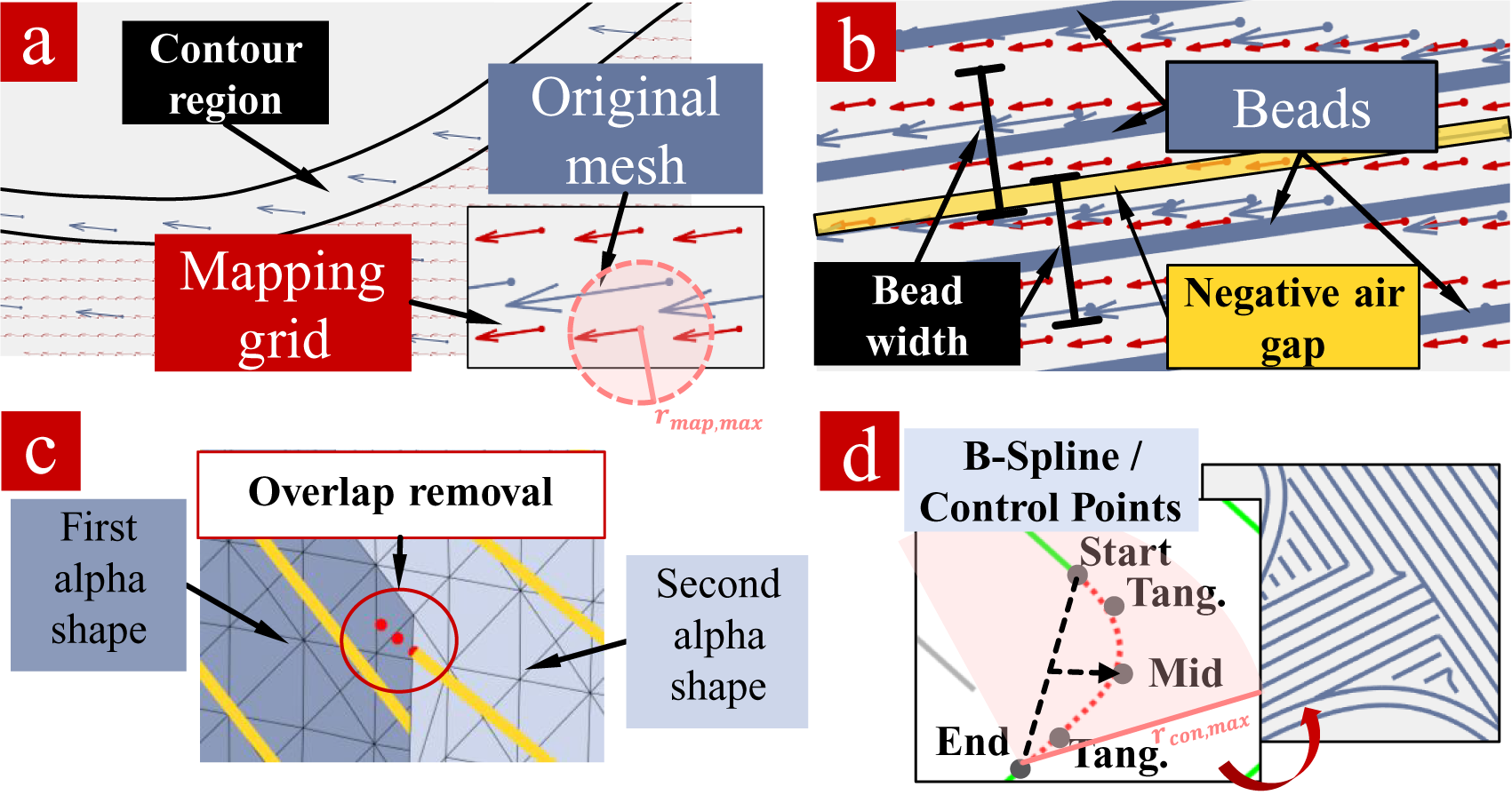
The vector field is now clustered by a K-means clustering algorithm (MacQueen Reference MacQueen1967) into regions of similar orientation according to an angle difference threshold. Multiple different K’s (number of clusters) are checked, and the one with largest silhouette coefficient (Rousseeuw Reference Rousseeuw1987) as quality criterion is used. The individual subsections of the vector field are then approximated by equidistant line segments, which form the later extrusion beads. Therefore, the line width corresponds approximately to the extrusion width of the FLM printer. To realize a negative air gap (bead overlap), it is chosen 8.33 percentage points smaller (0.55 mm instead of 0.6 mm) as an air gap of −0.05 mm lies within the strength-increasing range researched by Ahn et al. (Reference Ahn, Montero, Odell, Roundy and Wright2002) (see Figure 5b). The negative air gap is favourable for mechanical properties related to the polymer sintering process which occurs during FLM printing (Ahn et al. Reference Ahn, Montero, Odell, Roundy and Wright2002; Chakraborty, Aneesh Reddy & Roy Choudhury Reference Chakraborty, Aneesh Reddy and Roy Choudhury2008; Turner, Strong & Gold Reference Turner, Strong and Gold2014). After that, these individual line segments are postprocessed to remove grid-related remaining small overlaps with contour paths and other line segments (Figure 5c), then assigned to nearest neighbour lines and connected using B-Splines to avoid interruptions of extrusion paths (Figure 5d). For this B-Spline interpolation, five control points are used: (1) start point; (2) end point; (3) midpoint (‘Mid’) and (4) and (5) two control points for tangential condition (‘Tang.’). The midpoint is constructed by shifting the midpoint between the start point and the end point by half of their distance in average direction of both paths (dashed line and arrow). Tangential control points are extended from the two paths’ directions by a chosen fraction (here:  $ \frac{1}{3} $) of the midpoint’s shift. Implementation of infill path generation is described in Algorithm 1.
Algorithm 1. Pseudocode of the infill path generation algorithm; search radii are demarked in Figure 5a,d.
Input: Vector field of element centroid/optimized material orientations
Input: Assignment of el. centroids and material orientations to clusters
Input: Parameter  $ {r}_{map,\mathit{\max}} $: search radius for mapping
Input: Parameter  $ {r}_{con,\mathit{\max}} $: search radius for line segment connection
Start: Create a uniform grid:

Delete grid points outside of geometry and/or within perimeter regions
Create equidistant line segments within individual clusters as introduced in Voelkl, Kießkalt & Wartzack (Reference Voelkl, Kießkalt and Wartzack2019)
Assign lines to obtain continuous paths:

Derive trails of connected line segments: line segment trail
Connect lines:

Finally, the individual line segment trails (later printing paths) are sorted to minimize travel paths during printing, thus reducing build time. Specific requirements for this sorting to obtain FLM-suitable tours were laid out in Wasser et al. (Reference Wasser, Dhar Jayal, Pistor, Wasser, Jayal and Pistor1999). In literature about manufacturing, many elaborated algorithms exist (e.g., Yang et al. Reference Yang, Loh, Fuh and Wang2002; Han, Jafari & Seyed Reference Han, Jafari and Seyed2003; Fok et al. Reference Fok, Cheng, Ganganath, Iu and Tse2019). For this reason, sorting is regarded as a ‘black box’. Here, merely a simple solving solution for this variation of the Traveling Salesman Problem (TSP; Wasser et al. Reference Wasser, Dhar Jayal, Pistor, Wasser, Jayal and Pistor1999) is used, the Nearest-Neighbour-Heuristic. In this algorithm, from an initial starting or end point of a line segment, the closest (smallest Euclidean distance) starting or end point of all other line segments is connected. This process is repeated from the other point of this connected line segment to all remaining start and end points, and so on subsequently, until all points are visited. By varying the initial point, different tours emerge and the result can simply be picked as the best of all tours as measured by least travel way. The TSP heuristic usually leads to a ‘dead end’, that is, not closing the TSP tour (i.e., the traveller will not end up at his start point). However, this behaviour seems tolerable for FLM path planning; in turn, the heuristic is very efficient (Wasser et al. Reference Wasser, Dhar Jayal, Pistor, Wasser, Jayal and Pistor1999) and typically delivers a solution within seconds in this approach.
3.4. Simulation
To compare the design outcome of the approach and infill patterns generated by conventional slicing software, a simulation approach is used. This simulation approach was presented and also scrutinized for mesh dependency in Völkl, Mayer & Wartzack (Reference Völkl, Mayer, Wartzack, Lachmayer, Rettschlag and Kaierle2020). The approach is based on mapping material locations to FEs (empty regions will not be assigned) and material orientations to element coordinate systems in an FE simulation. Orthotropic FLM material models like these reviewed in Brenken et al. (Reference Brenken, Barocio, Favaloro, Kunc and Pipes2018) can then be used to obtain preliminary stiffness and strength results. Thus, different infill and contour setups can be compared.
4. Application of the method and results
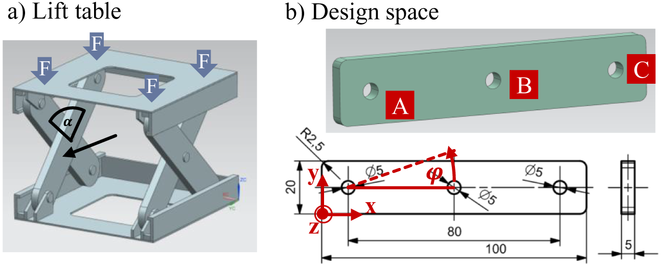
To demonstrate the capabilities of the approach, the geometry of a lifting arm (black arrow in Figure 4a) of a laboratory scissor lifting table is used. For this demonstrator, under different lifting heights, various loads on the part’s load introductions occur. This makes it an interesting case for multi-LC TO. Loads were calculated for an angle between the lifting arms of  $ \alpha =90{}^{\circ} $ for both lifting arms of an ‘X’ couple. The total load applied to the upper part of the table (F) is 10 N. Simulations are conducted using the FE software ANSYS (ANSYS, Inc. 2020) controlled by MATLAB (The MathWorks, Inc. 2020).
Table 2 gives detailed force and boundary information on three LCs: LC 1 – loads occurring under  $ \alpha =90{}^{\circ} $ on the first arm; LC 2 – the same, but for the second arm (applied to the same geometry to be able to interchange arms); LC 3 – misuse LC, load introductions A and C are fixed and a force in the z-direction at load introduction leads to bending. LC 1 and LC 2 were transformed into the red coordinate system shown in Figure 6. The third LC was chosen to demonstrate the approach’s capability to cope with multiaxial and through-thickness stress states and simulates a push from the side.
Applied boundary conditions and loads in different load cases

Introduction of demonstrator. (a) Lift table. (b) Design space.
For meshing the part, 11,814 SOLID186 elements were used in 12 layers of equal height to cover the height of the part (5 mm), so about one element height for two FLM layers. As mentioned in the methods section, the result of the DfAM approach is mesh dependent, as a finer mesh in both the z-direction and within the XY plane will deliver a better resolution of occurring stress states and also influence contours. More on this issue is presented in a mesh dependency study in the TO (the mesh dependency in topology optimization section) and path generation (Section 4.3).
4.1. Load-path-dependent build orientation optimization
For build orientation optimization, all PNSTs and magnitudes for each element and LC are collected (Section 3.1). These build the basis for the procedure of calculating angle differences to the printer’s XY plane. Subsequently, the angle differences are weighted using the absolute stress magnitudes. Weighted angle differences are then used in the optimization routine. All PNSTs of all LCs are shown in Figure 7a. Tension PNSTs are demarked in red and compression PNSTs in blue. Observing both the top and side views, it becomes obvious that most PNSTs are within the XY plane of the coordinate system shown. However, LC 3 also provokes stress trajectories through thickness. The optimization routine options – minimizing mean, median, mode and sum of weighted angle differences – are now applied. As a result, both mean and sum of weighted angle difference minimization deliver the same result vector for the optimized printer z-axis  $ \left({x}_z,{y}_z,{z}_z\right) $: $ \left(4.60\times {10}^{-8},-5.21\times {10}^{-8},1\right) $ (mean) and $ \left(5.08\times {10}^{-9},-1.52\times {10}^{-8},1\right) $ (sum). Both of these are very close to $ \left(\mathrm{0,0,1}\right) $. In contrast, median will deliver $ \left(0.32,-\mathrm{0.23,0.92}\right) $. Mode uses a GA for minimization, and there is a random influence.
Results of build orientation optimization. (a) Principal stress trajectories for all load cases. (b) Histogram of principal stress magnitude-weighted angle differences after optimization under four different objectives.

Thus 10 optimizations with different random seeds were run, and the best result z-vector reached is presented:  $ \left(-0.09,-\mathrm{0.35,0.15}\right) $. These determined vectors representing the printer’s z-axis in the part coordinate system are now used for evaluation. This z-axis is also the normal vector for the printer’s XY plane. For each of the results, weighted angle differences to the optimized XY plane are obtained from the last iteration of the optimization. These can then be displayed in a histogram (Figure 7b). On the x-axis, bins of a certain weighted angle difference according to the model are created, with 0.1 deg $ \cdot $MPa in steps of 0.1 deg $ \cdot $MPa to 2 deg $ \cdot $MPa, and another bin for larger differences. Mean and sum show most weighted angle differences in the first, low weighted angle difference and thus favourable bin (A, 76,278 of 106,326 weighted differences, 71.7%) and a rather small number in the outer right bin (B, 5432 weighted differences out of 106,326, corresponding to 5.1%), which represents higher weighted differences. In contrast, median shows just 43,149 differences in the ‘good’ bin (40.6%) and 20,673 in the ‘bad’ (19.4%). The minimization of weighted angle differences’ mode obtains 73,208 differences (68.9%) in the first bin, however, 18,042 in the outer right bin (17.0%). Thus, median and mode both show a higher number of larger weighted angle differences than mean and sum, indicating that their optimized direction does not ensure a plane load path like the z-axis derived from mean and sum. In bins in-between, a relatively small number of weighted angle differences can be found. Analysing average weighted angle difference, mean and sum obtain 0.36 deg $ \cdot $MPa, median 1.16 deg $ \cdot $MPa and mode 0.66 deg $ \cdot $MPa. Thus, the build orientation derived from mean and sum (the same result) is used for the following TO.
4.2. Topology optimization
To obtain an optimized geometry and inner material orientations for the LCs, the TO algorithm described in Section 3.2 is used. The volume fraction (the remaining section of design space) was chosen to 40% to obtain a result which allows to visibly draw conclusions about material distribution. In engineering context, volume fraction could also be made a variable dependent on a target stiffness or similar, which could lead to much finer or coarse structures. This is also supported by the approach. The example was optimized using an orthotropic material model of FLM-printed ABS-GF20 (ABS with 20 wt.-% GFs) according to Duty et al. (Reference Duty, Kunc, Compton, Post, Erdman, Smith, Lind, Lloyd and Love2017). Figure 8 presents the resulting structure.
TO result. (a) Alpha shape of isodensity nodes. (b) Pseudodensity distribution (translucency) and material orientations of whole structure. (c) Detail of fibre orientation results of different load cases.

Figure 8a shows the plotted alpha shape encompassing all elements with a pseudodensity larger than 0.2. A top and bottom layer can be identified in outermost distance to each other within the design space, mainly assigned obviously to LC 3. The top and bottom layer shape is influenced by the bending around the z-axis (yellow arrows are merely indicative). Figure 8b is a top view of the result, making the inner structures visible and allowing a view onto hollow parts around the two holes between top and bottom layers. Moving into detail view (Figure 8c), the MPNST vectors become visible, with different colours for the three LCs. These MPNSTs are projected into the XY plane (during iterations and at the end).
Determination of unique material orientation
As explained in the methods section, each element now shows three different MPNST vectors, one for each LC. For later path generation, a single direction per element has to be determined, which is done by two ways (Sections 3.2 and 3.3): (1) checking if a single LC’s orientation field is suitable for the other two, for all three LCs, respectively, and (2) choosing the MPNST of all three LCs as a compromise.
To compare the approaches, the final TO result was used and directly recomputed for all LCs, one by one for each of the fibre orientations. The quality of a single solution was determined by strain energy, where lower strain energy means better results.
Figure 9a shows the results (stiffness loss) for the single LC orientation and Figure 9b compares the ‘maximum’ approach to the individually optimized results.
TO result. (a) Comparison of different strain energy results (normalized to solution optimized for particular load case (LC). (b) Comparison of material orientation as ‘MPNST of all LCs’ to individually optimized solutions.
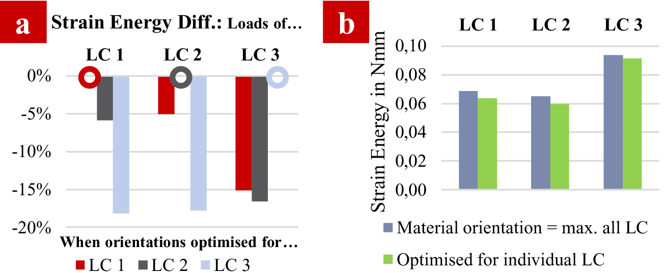
In Figure 9a, the x-axis demarks the different LCs applied to a structure with a material orientation setting of the corresponding LC and the other two, respectively. Different material orientation settings are symbolized by colours. The y-axis shows the percentage difference of the best strain energy for each LC/material orientation combination to a material orientation setting’s strain energy. For example, when applying LC 1 to models with material orientations which were optimized for LC 1, 2 and 3, respectively, total strain energy is 0.0637 Nmm (LC 1), 0.0671 Nmm (LC 2) and 0.0750 Nmm (LC 3). The best result characterized by lowest strain energy expectedly occurs when using LC 1’s optimized orientations when LC 1 is (rightly) applied. This leads to 0% deviation from best result (red circle in Figure 9a). Thus, the strain energy of LC 1 is  $ 0.0637/0.0671-1=-5.067 $% lower than strain energy obtained with LC 2’s orientations. For all LCs, the material orientation combination which was optimized for that particular LC delivers the best strain energy result. When material orientation settings of LC 2 under the loads of LC 1 and vice versa are compared, not much strain energy impact is observable. This is in agreement with the fact that both of them are nearly symmetric (except for the midload introduction, which is due to taking both lifting arm loads into one optimization setup) and under plane loading. On the other hand, comparing material orientation settings optimized for LC 3 under LC 1- and LC 2-loads and vice versa, differences in strain energy by using the inappropriate material orientation setting are large. This can be explained by the widely differing MPNST as introduced in Figure 7: LC 1 and LC 2 contrasted to LC 3 show largely differing optimized directions and are therefore not suitable to be covered by one another’s material orientation setting. Thus, a compromise should be found, which is depicted in Figure 9b. Using the locally prevailing LC’s stresses (MPNST for each element), a more homogeneous strain energy comparison emerges. For all of the LCs, the compromise solution is worse than the specifically optimized material orientation combinations (strain energy is larger). However, loss against optimized strain energy is −7.3% for LC 1, −8.1% for LC 2 and −2.3% for LC 3 compared to the losses in Figure 9a. LC 3 is the dominating LC overall (largest strain energy), which is depicted in the smallest loss against its optimized orientation (and also in the formation of the top and bottom layers in Figure 8). This compromise material setting is used for the path generation in the following.
Mesh dependency in topology optimization
As mentioned at the beginning of the result section, the optimization approach shows mesh dependency. Larger FEs lead to rougher results in contour and local stress resolution. This mesh dependency is studied here further.
The demonstrator is meshed using FEs with an edge length ranging from 0.5 mm (rather fine mesh) over 1 mm to 2 mm (very coarse mesh with just three layers over thickness). Figure 10 illustrates the results.
Effect of mesh resolution on (a) strain energy and (b) TO result in general (Minimum Member Size Filter is applied).

A coarser mesh delivers an increase in total strain energy for all three LCs (Figure 10a). This first implies a stiffer optimization result for finer mesh and also a higher resolution of local stresses. As these form the basis for the following step, path generation will also be affected. This is detailed further at the end of Section 4.3. Regarding TO results, strain energy goes up 3.7% and 17.2% for LC 1, 3.5% and 20.1% for LC 2 and 5.0% and 11.7% for LC 3, when increasing mesh edge length from 0.5 mm to 1 mm and from 0.5 mm to 2 mm, respectively. As known from FE theory, there is a convergence in its results when increasing mesh refinement (except for singularities), which is also depicted in decreasing percentage differences to the finest mesh resolution here. Recommendations for mesh resolution are given in the discussion section.
Effect of maximum principal normal stress projection in topology optimization
PNSTs are projected into the printer’s XY plane as described in the methods section. Through this, FLM material properties are depicted in the way they occur in the part later. This subsection will go into detail to scrutinize the influence of the MPNST projection on TO results.
Figure 11a shows the results of simple demonstrator chosen for easier understanding of the influence of projection. The lower part of the design space is fixed, a force acts in the drill hole on the upper left as shown. The drill hole must remain during optimization, that is, elements around it are fixed and it is nondesign space. The demonstrator is optimized without projection (left) and with projection into the XY plane (right) of the PNST. To obtain larger differences in comparison, no build orientation is conducted and the orientation as shown in Figure 11a is used. Thus, more load is transferred through the less stiff planes. This is for demonstration purposes only. Figure 9b gives corresponding strain energy results.
Effect of projection on (a) TO result and (b) strain energy.

The overall topology appears quite similar (Figure 11a, left and right). However, there are some crucial differences: On the left side of the part, close to the coordinate system, a massive strut in the z-direction emerges for the unprojected part with PNST also pointing along its longitudinal axis. This strut is very weak in the projected version and PNSTs are – due to projection – within the XY plane. Second, for the projected part, the diagonal strut in the XZ plane is much broader and has a flatter angle, probably as similar loads have to be transferred through the much less stiff z-direction. Figure 11b then shows that the unprojected version is much stiffer than the projected version [however, this cannot be manufactured by conventional FLM; see discussion (Section 5.2)]. When using the unprojected result and afterwards applying the FLM-based projected material orientation, strain energy increases; the projection-optimized result is favourable when conventional FLM is employed. Figure 12 goes into more detail on the geometries by subtracting the results’ pseudodensities. Blue dots indicate that the projected result has less material than the unprojected, and red dots indicate vice versa. Differences in pseudodensities between −0.1 and 0.1 are omitted for better visualization. It becomes obvious again that the strut in the z-direction is much more pronounced for the unprojected version (blue dots; detail A in Figure 12). At the same time, the projected result’s small diagonal strut in the XY plane is broader (more material, red) than the strut of the result from unprojected TO.
Comparing geometry in detail.

4.3. Path generation
Path generation is done in two ways for the given demonstrator part. First, the approach presented in methods section is used directly: derivation of contours, smoothing of contours and infill generation by filling the regions inside the perimeters with infill paths approximating the clustered PNSTs. The result is given in Figure 13.
Path generation result. (a) Extrusion paths of top, mid and bottom layers. (b) Overall structure in Raise3D ideaMaker software (Raise3D Technologies, Inc. 2020).

Figure 13a shows the top layer (layer number 1), one of the midlayer (12) and the bottom layer (25) extrusion paths derived from the ‘maximum of all LCs’ approach including two smoothed contour lines (moving average of two consecutive points). As desired for a 100% infill, the layers are properly filled. Connection between individual paths has been ensured by assignment of start- and endpoints and B-Spline interpolation (see detail in Figure 13a). A G-Code generating algorithm has been implemented to provide an interface to most common slicer software like ideaMaker (Raise3D Technologies, Inc. 2020; Figure 13b).
The travel (nonprinting) paths were minimized by the Nearest-Neighbour-Heuristic, leading to about −85.6% travel path reduction overall against the sorting order emerging from the path generation routine (from 3390.91 mm of unproductive travel to 488.55 mm), which is shown in Figure 14.
(a) Unsorted and (b) sorted paths.

For actual printing, support structures are added by using support paths from a slicing software which were generated using an STL model of the alpha shape of the path generation result. This approach leads to a fast and straightforward design of the part and directly usable manufacturing information. However, obviously, there is still room for improvement: Outer contours are smoothed; nevertheless, the initial TO shape remains visible with ‘steps’ dependent on mesh coarseness and smoothing (Figure 13a). The result geometry is not directly importable to common CAD systems. To increase visual appearance, allow for later modification and function integration, the result can be manually or (semi)automatically (Stangl & Wartzack Reference Stangl, Wartzack, Weber, Husung, Cascini, Cantamessa, Marjanovié and Rotini2015) retransformed into CAD geometry. A manually reconstructed version of the part using Siemens NX is presented in Figure 15. Such a restructured version can be directly processed by a slicing software to derive building source. Exemplarily, lattice structures in the inner compartment were generated, which have already been used in other work for energy absorption and buckling reduction, and can be optimized further for anisotropy (Iyibilgin, Yigit & Leu Reference Iyibilgin, Yigit and Leu2013; Sui, Fan & Lai Reference Sui, Fan and Lai2015; Stanković, Mueller & Shea Reference Stanković, Mueller and Shea2016). Optimization and scrutiny of lattice structures is outside the scope of this approach. Integration of lattice structures is demonstrated here as a possible way of extension (Figure 15).
Reconstructed optimization result and transfer to slicing software with concentric infill.

4.3.1 Mesh dependency in path generation
Starting from TO, paths are generated and therefore share the mesh dependency. For the coarse mesh of 2 mm (Figure 10b), only three different mesh layers through thickness are generated, which leads to a less precise approximation of the optimized PNST by the generated paths. Figure 14a illustrates this influence qualitatively. Then, Figure 16b shows derived paths of layers 21 and 22 (0.2-mm layer height) from the optimization results in Figure 16a.
(a) Optimization results and (b) derived layers 21 and 22 in overlay view to illustrate differences.

Increasing mesh coarseness leads to repetitious paths between layers and overall coarser shape, which in turn leads to equal perimeters. An exception is between layers 21 and 22 on 1-mm mesh, where the red layer takes more area than the blue layer. This is due to the emergence of a different thickness of top and bottom structural plane elements, as their heights are restrained by mesh size, and one layer falls into the upper ‘belt’ and the next one in the middle section. Infill patterns are also less precisely adapted to PNST, as resolution of stress states is decreased. In Figure 16a, this behaviour is explained: The height of demonstrator (constant) is discretized using FEs (abstracted as grey cubes) and sliced always using the same number of layers (coloured horizontal lines). Each element exhibits a unique material orientation (the determination of unique material orientation section), which is mapped on all the layers that fall into its height on the z-axis, resulting in unchanged subsequent layers, as depicted by the differently coloured lines. The 2-mm mesh is very coarse for illustrative purposes only.
4.4. Simulations of FLM printable designs
Approximation of the actual optimization result by reconstruction might lead to a loss of lightweight potential exploited in two ways: First, the overall geometry is altered (e.g., position of holes, outer contour etc.). Second, the infill is not directly oriented within load-path orientation but determined by infill pattern. To scrutinize loss, structural FLM simulations were conducted for:
(i) Reconstructed geometry (without lattice) in optimized printing direction with concentric (shifting contours into the inner areas) infill;
(ii) The same as (i), but using lines ( $ \pm 45{}^{\circ} $) infill;
(iii) Printing in optimized printing direction for LC 3 with lines infill.

Infill patterns and simulation results are given in Figure 17. The simulation was conducted with a tetrahedral mesh and ABS-GF20 material parameters by Duty et al. (Reference Duty, Kunc, Compton, Post, Erdman, Smith, Lind, Lloyd and Love2017). The linear structural FE simulation uses orthotropic material models (orientation of material axes by element coordinate systems).
Simulation results for (a) concentric, (b) lines infill and (c) lines infill with ‘upright’ printed model. (d) Comparison of efficiency measure for the three options 1.–3.

Material models have to be derived for each parameter set of a printer. Figure 17a–c presents G-Code patterns: (a) Concentric infill, two walls, 0.2-mm layer height; (b) Lines ( $ \pm 45{}^{\circ} $) infill, other parameters likewise; (c) Upright printing (optimized orientation for LC 3) with lines infill, other parameters as in (a) and (b).
Figure 17d contains a chart with different volume-weighted strain energy results for the original TO result and all infill patterns and LCs. The lightweight efficiency measure is derived from Rozvany (Reference Rozvany2009) and originates from comparing topology-optimized structures’ exploited lightweight potential against Michell structures (Michell Reference Michell1904). Strain energy is multiplied by volume employed. A lower efficiency number thus indicates better exploitation of lightweight potential. To enhance its understanding, in this contribution, the reciprocal value is used; therefore, a higher number indicates better exploitation; the overall number for each LC is normed to 100% for the best result.
For all LCs, the initial TO result without any alteration in geometry or approximation of MPNST via infill, that is, just taking the optimized material distribution and orientation, yields the best efficiency figures and is taken as a benchmark. For LC 1 and LC 2, concentric infill obtains the second best results, with a loss of about 20 percentage points against the optimized solution. This relatively good result can be explained, as the concentric infill pattern actually provides a good approximation of optimized fibre orientations (Figure 18).
Oriented element coordinate systems from G-Code.

Moving to Figure 17d again, for LC 1 and LC 2, lines infill induces a further decline in the benchmark, and worst results are obtained for ‘upright’ printing. However, for LC 3, concentric is still better than lines infill; nonetheless, the originally optimized printing direction (dark grey bar) provides the best exploitation of material properties related to force flow.
Finally, Figure 19 shows a printed version of the optimized and reconstructed scissor arm using concentric infill, including lattice structures within the hollow regions in Figure 19b. Printing was done using a 0.6-mm hardened steel nozzle using 20-wt.-% CF reinforced PolyEthylene Terephthalate Glycol-Modified on a Raise3D Pro2 Plus Printer.
Printed scissor arm. (a) Surface concentric without ‘ironing’. (b) Surface ‘ironed’ and including lattice. (c) Upright view.

The printed part illustrates further possibilities in FLM printing: Figure 19a presents the whole demonstrator printed with 100% concentric top layer solid fill as simulated before. Figure 19b is printed using the ‘ironing’ feature of Ultimaker CURA (Ultimaker B.V. 2019), which does a surface finish by moving the hotend slowly over the top layer, therefore increasing surface quality. This might be desirable for both reducing surface stresses and improving optical appearance. Finally, Figure 19c gives a view of the non-‘ironed’ part in upright position to point out the top and bottom layers mainly driven by LC 3.
4.5. General applicability of the approach: manifold test cases
To demonstrate a more general applicability of the approach, multiple further test cases have been conducted. Each involves just one LC or two simple LCs to allow for convenient plausibility checking. These are shown in a full page (Figure 20). The design space and load direction is depicted in red, resulting alpha shapes after build orientation in blue and a selected number of layers in ascending order in black detail frames. Selection of layers was done to illustrate differences in varying printing heights.
Application of the approach to other test cases. A.1 and A.2: simple two-cube demonstrator under two load directions. B.1: more complicated design space. C.1: plate demonstrator under single load. C.2: the same demonstrator under symmetric load.
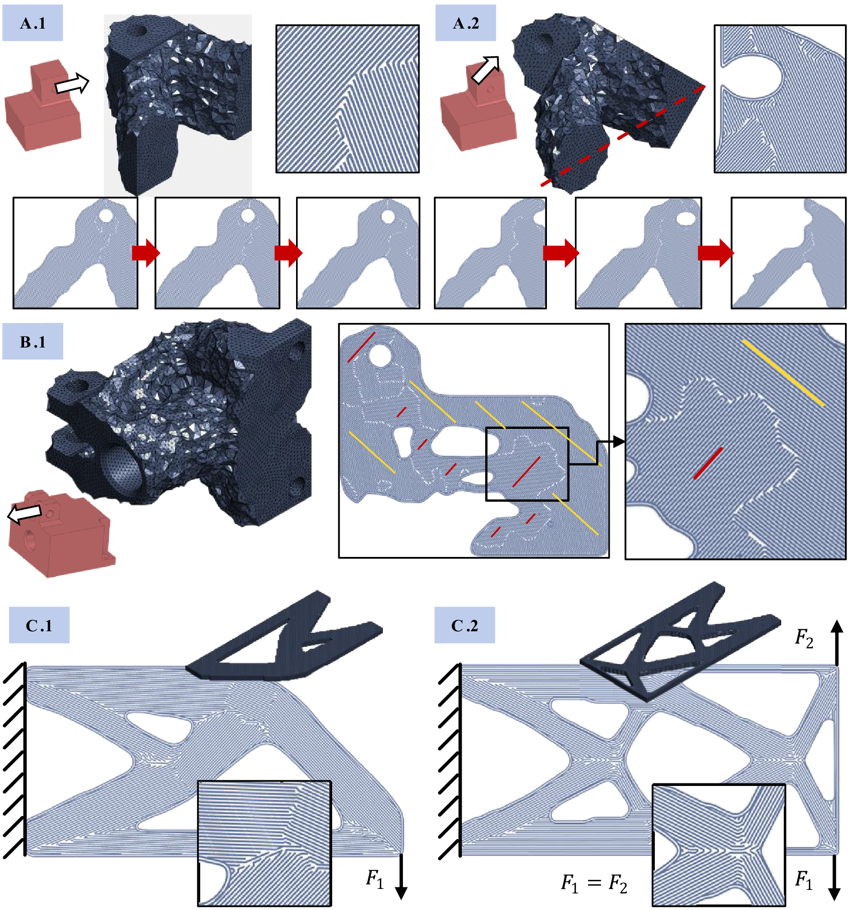
Demonstrator A was optimized for a simple force LC (A.1) and under a diagonal force load (A.2). The result of A.1 shows that largely unstressed areas of the cube are removed (lower right), and the load is transferred into the fixed support via two main struts. Build direction optimization yields a flat orientation which allows for the force flow to remain largely in-plane. Principal stress trajectories align with the tension and compression struts.
For result A.2, the force direction provokes build orientation to be at  $ 45{}^{\circ} $ to the design space outer boundary plane. Thus, force flow again stays in-plane with extrusion paths pointing towards the hole. Extrusion orientations follow largely along the struts. Demonstrator B.1 shows that the new approach is capable of handling more complicated geometry and design space restrictions. There is a tunnel in lengthwise direction which must not be used as design space, and its walls have to remain. The same applies for the screw holes at the back, as these form the load introduction. The force load provokes extrusion orientations which are orthogonal to each other, depicted in red and yellow. Due to the more varying load path, also more complicated extrusion paths patterns evolve.
The third demonstrator (C.1 and C.2), a plate under single load and symmetric load on both sides, is a typical TO example. It demonstrates the symmetry which the new approach keeps throughout processing. Material orientations again align with force flow and are continuous throughout the part, also at geometric discontinuities. However, as shown in the detail of C.2, printing orientations are sometimes orthogonal to load directions, which is owed to the perfectly symmetrical LC. If one LC would prevail, this would lead to continuous material orientations (similar to C.1). This issue is commented on further in the discussion.
All of the manifold test cases above are quantitatively scrutinized further. This study encompasses the following alternatives for each demonstrator A.1, A.2, B.1, C.1 and C.2:
(i) This contribution’s TO of the presented approach, applied directly;
(ii) The same, but including subsequent path generation;
(iii) ANSYS TO routine with the same optimization settings as the TO presented here, with concentric infill pattern applied subsequently using Raise3D ideaMaker (Raise3D Technologies, Inc. 2020);
(iv) The same ANSYS TO routine, but with
$ \pm 45{}^{\circ} $ infill pattern.

These alternatives intend to give a comparison of pure TO including optimized material orientations (i) with the respective impact on strain energy when approximating the optimized material using path generation (ii). Furthermore, a comparison with another optimized topology for each demonstrator (generated from ANSYS TO) and other infill patterns is conducted with (iii), concentric infill, and (iv)  $ \pm 45{}^{\circ} $ infill. Again, the efficiency measure in Figure 17 is used for comparison between the alternatives, obtained from the simulation approach presented in Section 3.4. Results are shown in Figure 21a.
Quantitative comparison of the optimized test cases. (a) Efficiency measure of TO result, path generation result, ANSYS TO result with concentric infill pattern and ANSYS TO result with  $ \pm 45{}^{\circ} $ infill raster. (b) Strain energy of TO results with fixed infill raster in steps of $ 10{}^{\circ} $ (for explanation, see C.1).
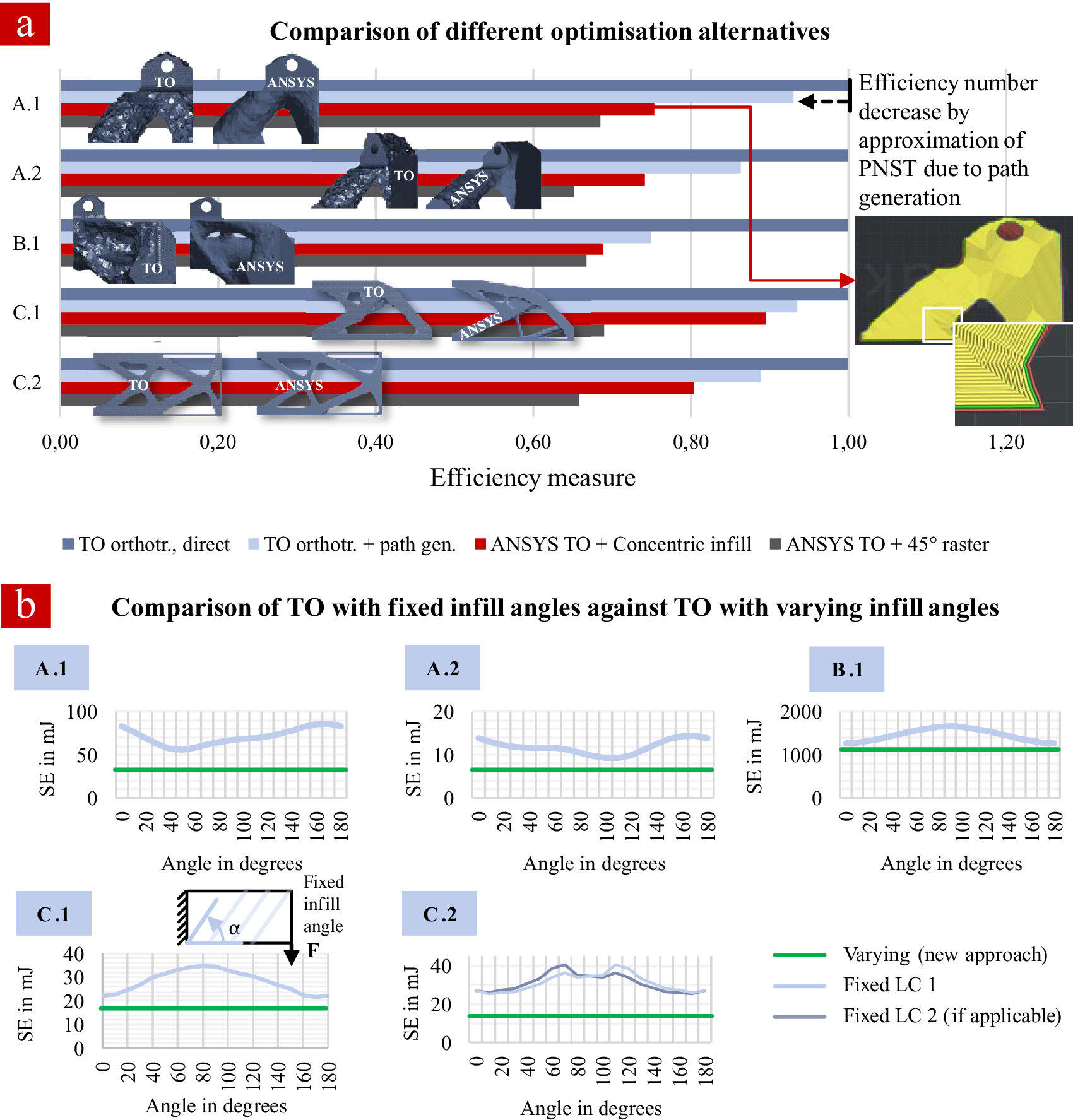
In addition to that, a further study on fixed infills during TO is conducted. The proposed TO algorithm is applied but with a predefined infill angle in steps of 10° from 0° to 180° instead of manipulating each element’s orientation according to PNST. This will return a geometry optimized for each specific infill angle with the same volume fraction. To compare these geometries, strain energy is used directly (volume stays the same). Figure 21b shows the fixed infill results (light blue) and compares these with the original result including material orientation optimization (green) for each demonstrator.
For all demonstrators, path generation decreases the efficiency number (strain energy times volume, inverted) against pure TO to various amounts, from about −6% (A.1 ‘cubes’ and C.1 ‘plate’) over −11% for C.2 (two LCs, mean of both strain energy results used) and −14% (‘cube diagonal’) to −25% (tunnel demonstrator; Figure 21a). For the simpler demonstrators in terms of both geometry and LCs, rather straightforward material orientations emerge, which can be depicted quite accurately by the path generation. More complicated load/geometry situations (C.2, A.2 and B.1) lead to less accurate approximation. The isotropic TO results from ANSYS (exported to STL with correct volume fraction, then preprocessed for FLM using ideaMaker) show much smaller efficiency measures. When compared to the path generation result of the new approach, which is also directly printable like the preprocessed ANSYS geometries, reductions of the measure lie between −4% (C.1) and −19% (A.1) for the concentric infill (see detail in Figure 21a) and even −11% (B.1) and −26% (A.1) for the  $ \pm 45{}^{\circ} $ infill. Regarding fixed infill in steps of 10°, simultaneous optimization of topology and material orientation is advantageous for all demonstrators, as it delivers lower strain energy in comparison to all angle steps (green line in Figure 21b). For all demonstrator-LC combinations, there is one favourable infill angle. For demonstrator C.1 (plate under bending), for example, this is 0° (180° is equivalent). For the two-LC example C.2, strain energy results are given for both LCs. The resulting strain energy chart is symmetric, like the geometry and the LCs. Best results are at 10° (LC 1) and 170° (LC 2). Correspondingly, for A.1, the best angle is 50°, that is, along the left strut in Figure 20. For A.2, it is 100° (based on the altered coordinate system, which means along the right strut Figure 20). Finally, for B.1, the best direction is along the tunnel (0°).
5. Discussion
The following section gives an in-depth discussion on the different parts of the optimization approach.
5.1. Discussion of build orientation optimization
Build orientation optimization aims to bring load paths as much as possible into the printer’s XY plane, as interlayer bonding is typically weaker than bonding between beads. Therefore, all principal stress trajectories and their magnitudes are considered: Angle differences between PNST and the build plane are calculated and weighted by magnitudes. Thus, smaller angle differences are weighted stronger if their magnitude is higher and vice versa. Large angle differences with large magnitudes have a high influence on the optimization results, and also vice versa. Best results were obtained when the mean of weighted angle differences was chosen as optimization objective. ‘Sum’ delivers the same result, as the number of elements did not change between LCs. Both median and mode delivered very different optimized solutions and less favourable orientations. Obtained optimized result vectors for the best solutions are in intuitive accordance with the LCs presented, as, for example, high bending stresses are transferred in-plane. Within the scrutiny of manifold test cases, build orientation optimization also yielded plausible results and is thus taken as the basis for the subsequent TO.
5.2. Discussion of topology optimization
TO is widely recognized in DfAM. The presented approach, like some others, offers the possibility to not only optimize the outer geometry, but also provide information about how to print the inner structure as a basis for FLM extrusion paths later. For multiple LCs, the problem of choosing the (one) optimal orientation locally under the different stress states provoked is not resolved completely in this contribution; however, with the ‘maximum’ approach, a heuristic compromise is proposed. This compromise leads to good approximation of the strain energy results obtained when using the optimized orientations for each particular LC. These orientations, optimized for stiffness, are used later on for extrusion path generation. This might be suboptimal as neighbouring elements, due to choosing maximum orientation, may have largely differing angles, which leads to printing path direction changes within a specific layer. This could possibly impact local strength. Further study should be conducted on the influence of abrupt direction changes in extrusion paths on strength, and how to build more strength-oriented paths, for example, using failure criteria established for FRP in general or specifically for FLM like Bellini & Güçeri (Reference Bellini and Güçeri2003) and Hill & Haghi (Reference Hill and Haghi2014). Mesh dependency and the influence of projected PNSTs were scrutinized. For mesh dependency, a separate discussion is given below. Projection of PNST has a high influence on optimization results. Projected results showed flatter angles of struts through-thickness. Unprojected PNSTs give the stiffest result. However, these are not easily manufacturable using conventional FLM, although currently research in the field of curved FLM is ongoing. Furthermore, using unprojected results and projecting afterwards is suboptimal, as was shown in Figure 11b. Therefore, the projection method is used and offers derivation of geometry propositions including the specific material behaviour of FLM.
5.3. Discussion of path generation
The presented path generation method shows both advantages and disadvantages: Resulting extrusion paths’ orientations are closely aligned with optimized material orientations. Depending on initial clustering of similar fibre orientation regions, the paths can be aligned tighter or more loosely to these orientations. B-Spline interpolation allows paths to be as long as possible. This avoids interruptions in material flow and local weakening. Negative air gap consideration is provided. Overall, the path generation and sorting algorithms are also implemented efficiently and based on relatively simple concepts, leading to near real-time path generation. However, resulting paths are not necessarily curved smoothly, but, depending on settings, can exhibit direction changes with small radii. This is a compromise as the infill density should be 100% to not alter the TO result in a negative way by introducing new holes. Furthermore, individual infill paths should overlap consistently, ensuring the negative air gap for better mechanical properties and being as uninterrupted as possible. Using streamlines as used for Automated Fibre Placement in Spickenheuer (Reference Spickenheuer2014) might provide smoother paths, however, exhibiting more local voids and/or interrupted, shorter paths.
A good approximation might be the concentric infill pattern according to the simulation studies, which offers smoothly curved paths, sufficient overlap and a close to 100% infill density. However, it still is a compromise in terms of uninterruptedness (where ‘contours shifted inwards meet’).
Further applicability of the approach was illustrated for both TO and path generation by more examples with varying geometrical intricacy and under single- and multiple LCs. Results first show that TO and path generation are stable also under more complicated requirements. Furthermore, for the intuitively understandable LCs A.1 and A.2, alignment of extrusion paths with struts seems logical. The others show plausible overall topology and path generation results, for example, with the given load leading to complete usage of the outer boundary of the design space (B.1) and the corresponding inner infill patterns. The demonstrator B.1 exhibits orthogonal load paths between the tension and compression areas (red and yellow in Figure 20). This behaviour is caused by the abrupt change between the largest principal normal stress from tension to compression. This could be improved on in the future and be achieved by additionally averaging the trajectories in certain regions (although this is not favourable for approximating optimized material trajectories). Symmetry was demonstrated using a simple plate demonstrator (C.1 and C.2). The symmetric demonstrator C.2 shows material orientations in the ‘joints’ between the ‘struts’ which are orthogonal to the load direction. Overall, no single LC prevails here and thus the presented material orientation emerges. For such cases, it could be advantageous to use a simpler infill pattern locally. For example, a  $ \pm 45{}^{\circ} $ infill pattern oriented properly could improve strength in such areas (Cantrell et al. Reference Cantrell, Rohde, Damiani, Gurnani, DiSandro, Anton, Young, Jerez, Steinbach, Kroese and Ifju2017). Finally, the five test cases were benchmarked against conventional TO results (isotropic) with subsequent assignment of infill ( $ \pm 45{}^{\circ} $ raster and concentric). Although the concentric infill led to better efficiency measures in all cases when compared to the $ \pm 45{}^{\circ} $ raster, it still was in most cases considerably lower when compared to the results of the new approach. Indeed, for the demonstrator B.1, results were quite similar, which presumably is because of the remaining tunnel geometry in the middle. This element bears much load and is at the same time primarily built up using 0° contours instead of infill in all path designs. For C.1 (plate under bending) and to a certain degree C.2, on the other hand, concentric infill and the optimized infill of the new approach largely coincide. In the ‘cube’ cases A.1 and A.2, the efficiency gain of the new approach is clearly visible. Optimized infill patterns differ largely from the concentric infill (detail in Figure 21 against A.1 in Figure 20).
5.4. Recommendations on mesh resolution
Mesh dependency affects the approach in all FE-based parts. To obtain best possible results, mesh resolution can be set to layer thickness of the FLM printer – as this is the maximum resolution achievable by the manufacturing process. If nozzle width is still smaller than layer height, the mesh should be generated this fine. However, in practice, approximating the ‘ideal’ mesh resolution, for example, by increasing refinement in a convergence study, is more suitable to avoid high computation times and still obtains a suitable compromise between optimization/path generation quality and time required. In addition, singularities and depiction of fine geometry details should also be considered, as it is always necessary in FE model building.
5.5. Discussion of simulation of FLM optimized parts
Simulation of FLM parts is challenging and largely dependent on FLM machine parameters. Many simulation approaches exist. In this study, a straightforward simulation approach was used, which maps local G-Code orientations on an FE model and conducts the simulation using an orthotropic material model from literature. It is meant to give a rough estimate and, through that, first recommendations on favourable and less favourable build orientation and infill patterns. For a specific application, this kind of simulation has to be fine-tuned by material models derived from a specific printer configuration encompassing both stiffness and strength properties.
5.6. Concluding remarks
In this work, a novel approach for the design of load-path-dependent FLM structures was introduced. The holistic approach encompasses multiple different optimization and postprocessing procedures from design space to the completed part, taking the highly anisotropic nature of FLM parts into account. It addresses shortcomings of existing approaches, as it is able to directly optimize individual infill paths for stiffness. This is opposed to isotropic TO and using conventional rasters, setting a fixed angle raster as prerequisite for optimization or using smooth yet not specifically optimized isolines of Level-Set results. A promising extension of the approach presented could encompass more detailed depiction of FLM material behaviour considering individual printing settings. Build orientation or local TO criteria can be modified accordingly. Mesh dependency remains a major challenge for FE-based approaches in general, as it limits design capabilities, which actually could be exploited by the accuracy of FLM printers. For the proposed approach, a mesh dependency study has been conducted and a convergence study starting from coarse to finer meshes is recommended. The approach generally addresses a design-focussed view instead of the primarily production-based view mirrored in many approaches such as support structure or overhang optimization. A combination of both views could be interesting for achieving a symbiosis between manufacturability and structural optimality.
Glossary
ABS Acrylonitrile Butadiene Styrene
AM Additive Manufacturing
BESO Bidirectional Evolutionary Structural Optimization
CAD Computer-Aided Design
CAE Computer-Aided Engineering
CAIO Computer-Aided Internal Optimization
CF Carbon Fibre
DfAM Design for Additive Manufacturing
DoO Degree of Orthotropy
E Young’s Modulus
FDM Fused Deposition Modelling
FE Finite Element
FLM Fused Layer Modelling
FRP Fibre Reinforced Plastics
GA Genetic Algorithm
GF Glass Fibre
LC Load Case
MPNST Maximum Principal Normal Stress Trajectory
PETG PolyEthylene Terephthalate Glycol-Modified
PLA PolyLactic Acid
PNST Principal Normal Stress Trajectory
SKO Soft Kill Option
TO Topology Optimization
TSP Traveling Salesman Problem
UTS Ultimate Tensile Strength
Acknowledgments
The authors would like thank Jan Hinrichsen, B.Sc., student at Engineering Design, FAU Erlangen-Nuremberg, for his contribution to the 3D TO source code, and Johannes Mayer, M.Sc., research assistant at Engineering Design, FAU Erlangen-Nuremberg, for his contribution to the FLM simulation approach, as well as Michael Franz, M.Sc., likewise, for his inspiration in the path generation algorithm. We especially thank Fabian Buettner, B.Sc., for his support in the study of manifold test cases.


 Open access