


1. Introduction
This paper is concerned with investigating the consequences of introducing the Maxwell–Cattaneo (M–C) transport effect into the study of double-diffusive convection. Almost all previous studies of thermal convection, as well as more elaborate models involving magnetic fields, double diffusion, etc., use the classical Fick's law to describe the relation between quantities such as, for example, temperature and heat flux. For temperature, this relation (known as Fourier's law in this specific case) takes the form  $\boldsymbol q = - K \boldsymbol \nabla T$, where $\boldsymbol q$ is the heat flux, $T$ is the temperature and $K$ is the thermal conductivity. The Fourier law predicts an instantaneous response of temperature to the heat flux gradient, leading to a parabolic diffusion equation for the temperature field. The instantaneous response at all points implied by this equation cannot be exactly correct as information must travel at a finite speed. This weakness was recognised by Maxwell (Reference Maxwell1867) in his study of the theory of gases, who proposed a modified equation incorporating a finite relaxation time. Cattaneo (Reference Cattaneo1948) proposed a similar relation for solids, which was developed further by Oldroyd (Reference Oldroyd1950). Other important contributions were made later, by, for example, Fox (Reference Fox1969) and Carrassi & Morro (Reference Carrassi and Morro1972).
The idea of a finite relaxation time is incorporated into the M–C relation in the temperature equation between the heat flux  $\boldsymbol q$ and the temperature $T$, which then takes the form
 \begin{equation} \tau_{T}\frac{\mathcal{D} \boldsymbol q}{\mathcal{D} t} ={-} \boldsymbol q - K \boldsymbol \nabla T,\end{equation}
in which  $\tau _{T}$ is the relaxation time. The operator $\mathcal {D}/\mathcal {D}t$ here denotes a generalised Lagrangian time derivative, which should be chosen to give expressions that do not depend on the frame of observation; a specific form of this generalised derivative is discussed in § 2.1. The importance of the thermal relaxation term is typically expressed via the dimensionless M–C coefficient ${C_{T}}$, which is defined as the ratio of the thermal relaxation time to twice the thermal diffusion time; i.e. ${C_{T}} = \tau _{T} K / (2 \rho c_p d^{2})=\tau _{T} \kappa /2 d^{2}$, where $\rho$ is the density, $c_p$ the specific heat at constant pressure, $d$ a representative length scale and $\kappa$ the thermal diffusivity. (The factor of two in the denominator of the expression for ${C_{T}}$ does not seem to be particularly helpful. However, it is the definition of ${C_{T}}$ used previously in the literature, which we therefore choose to retain for consistency.) Thus the classical Fourier law has ${C_{T}}=0$. The introduction of a finite relaxation time changes the fundamental nature of the parabolic heat equation of Fourier fluids, in which heat diffuses with infinite speed, to a hyperbolic heat equation with a solution in the form of a heat wave that propagates with finite speed (Joseph & Preziosi Reference Joseph and Preziosi1989; Straughan Reference Straughan2011a).
The M–C heat transport effect has been studied in a wide variety of different physical contexts: for example, in solids (Barletta & Zanchini Reference Barletta and Zanchini1997), in fluids (Lebon & Cloot Reference Lebon and Cloot1984; Straughan & Franchi Reference Straughan and Franchi1984; Straughan Reference Straughan2009, Reference Straughan2010; Stranges, Khayat & Albaalbaki Reference Stranges, Khayat and Albaalbaki2013; Bissell Reference Bissell2015; Stranges, Khayat & deBruyn Reference Stranges, Khayat and deBruyn2016; Eltayeb Reference Eltayeb2017), in porous media (Straughan Reference Straughan2013; Haddad Reference Haddad2014), in nanofluids and nanomaterials (Jou, Sellitto & Alvarez Reference Jou, Sellitto and Alvarez2011; Lebon et al. Reference Lebon, Machrafi, Grmela and Dubois2011), in liquid helium (Liepmann & Laguna Reference Liepmann and Laguna1984; Donnelly Reference Donnelly2009), in biological tissues (Dai et al. Reference Dai, Wang, Jordan, Mickens and Bejan2008; Tung et al. Reference Tung, Trujillo, Lopez Molina, Rivera and Berjano2009) and, in the context of magnetoconvection, in stellar interiors and the solar photosphere (Bissell Reference Bissell2016; Eltayeb, Hughes & Proctor Reference Eltayeb, Hughes and Proctor2020). The potential significance of the M–C effect depends on a number of factors, through the definition of the coefficient  ${C_{T}}$. In gases, the relaxation time $\tau _{T}$ can be as small as picoseconds; ${C_{T}}$ will then only assume $O(1)$ values over very small scales, as can occur for heat transport in nanostructures. Nonetheless, even if ${C_{T}} \ll 1$, the M–C effect can still be important if the thermal driving (measured by the Rayleigh number, for example) is extremely high; this is often the case in astrophysical settings. In biological matter, the situation can be quite different, since $\tau _{T}$ can be of the order of a second or greater; the M–C effect can then be important on everyday length scales.
In this paper we study the consequences of including the M–C effects on the onset of double-diffusive convection, in which two quantities affect the density of a fluid,but diffuse at different rates. There are now M–C effects to be considered for both temperature and salinity. The most widely studied example of double diffusion is thermohaline convection, in which the competing ingredients are heat and salt, with the diffusion of heat greatly exceeding that of salt. Here we shall stick to the terminology of ‘heat’ and ‘salt’, although the equations are relevant in a much wider context. On including the M–C salinity effect, the modified salinity evolution equation can be obtained by analogy with the temperature equation, so can be written as
 \begin{equation} \tau_{S} \frac{\mathcal{D} \boldsymbol q_{S}}{\mathcal{D} t} ={-} \boldsymbol q_{S} - \kappa_{S} \boldsymbol \nabla S,\end{equation}
where  $S$ is the salt concentration, $\kappa _{S}$ the saline diffusivity, $\tau _{S}$ the relaxation time for salinity and $\boldsymbol q_{S}$ the salt flux. We note that the relation between salt flux and salt concentration differs from that between heat and temperature; hence the appearance of $K$ in (1.1) but $\kappa _{S}$ in (1.2). For later use we define the M–C coefficient for salt as ${C_{S}}=\tau _{S} \kappa _{S} /2 d^{2}$.
Double-diffusive convection has been widely studied for many decades in a variety of geophysical, astrophysical and engineering contexts (see, for example, the reviews by Turner (Reference Turner1974), Huppert & Sparks (Reference Huppert and Sparks1984), Turner (Reference Turner1985), Schmitt (Reference Schmitt1994), Garaud (Reference Garaud2018) and the monograph by Radko (Reference Radko2013)), but principally employing the Fickian law for the evolution of both diffusing ingredients. Herrera & Falcón (Reference Herrera and Falcón1995), via a fluid parcel argument, considered the new physics introduced by the thermal M–C effect (but with  ${C_{S}}=0$) into double-diffusive convection, motivated by heat transport in neutron stars and compact X-ray sources, where the competing gradients are of temperature and helium concentration. Straughan (Reference Straughan2011b) looked at this problem in more depth, but again restricted attention to the case of ${C_{S}}=0$ and for the case of a porous medium rather than a viscous fluid.
Motivated by geophysical and astrophysical considerations, we concentrate here on the case where the M–C coefficients are very small. The modified equations then represent singular perturbations in the time domain, and hence, even when  ${C_{T}}, {C_{S}} \ll 1$, new mechanisms for oscillatory instability can arise, provided that the initial gradients of temperature and salinity are very large. The goal of this paper is to investigate the effects of the new terms on the onset of instability in the regime of ${C_{T}}, {C_{S}} \ll 1$. The dependence of the results on ${C_{T}}$ and ${C_{S}}$ is very rich, so in this first paper we confine ourselves to the two special cases where one of the M–C coefficients is zero. The general case turns out to merit a second paper, which is in preparation.
The plan of the paper is as follows. In § 2.1 we demonstrate how the M–C effects can be incorporated into the equations describing the evolution of temperature and salinity; in § 2.2 we give the full set of governing equations for M–C double diffusion; § 2.3 presents the linearised stability problem for a basic state with linear gradients of temperature and salinity, with simple boundary conditions. In the two subsequent sections we investigate the special cases of  ${C_{S}}=0$ (§ 3) and ${C_{T}}=0$ (§ 4); for each of these we investigate the onset of linear instability for all combinations of the temperature and salinity gradients, concentrating on small values of the M–C coefficients and large values of the gradients. The significance of the results is assessed in the concluding section (§ 5).
2. Mathematical formulation
2.1. The M–C effect in a moving frame
To derive the governing equations, it is necessary to consider the modifications of the M–C effect to be expected in a fluid moving with velocity  $\boldsymbol u$. A number of possible formulations of the nonlinear terms have been proposed (e.g. Lebon & Cloot (Reference Lebon and Cloot1984) commenting on Straughan & Franchi (Reference Straughan and Franchi1984); Christov (Reference Christov2009)). Here we follow the formulation of Christov (Reference Christov2009), who proposed the following frame-invariant equation for the evolution of the heat flux:
 \begin{equation} \tau_{T} \left[\frac{\partial\boldsymbol q_{T}}{\partial t}+\boldsymbol u\boldsymbol{\cdot}\boldsymbol \nabla\boldsymbol q_{T}-\boldsymbol q_{T}\boldsymbol{\cdot}\boldsymbol \nabla\boldsymbol u+(\boldsymbol \nabla\boldsymbol{\cdot}\boldsymbol u)\boldsymbol q_{T}\right] ={-} \boldsymbol q_{T} - K \boldsymbol \nabla T. \end{equation}
It is convenient to write this equation as
 \begin{equation} \tau_{T} \left[\frac{\partial\boldsymbol q_{T}}{\partial t}-\boldsymbol \nabla\times(\boldsymbol u\times\boldsymbol q_{T})+(\boldsymbol \nabla\boldsymbol{\cdot}\boldsymbol q_{T})\boldsymbol u\right]={-} \boldsymbol q_{T} - K \boldsymbol \nabla T, \end{equation}
since, on taking the divergence, we obtain
 \begin{equation} \tau_{T}\left[ \frac{\partial {Q_{T}}}{\partial t}+ \boldsymbol \nabla\boldsymbol{\cdot}(\boldsymbol u \, {Q_{T}})\right]={-} {Q_{T}} - K \nabla^{2} T, \end{equation}
where  ${Q_{T}}=\boldsymbol \nabla \boldsymbol {\cdot }\boldsymbol q_{T}$ and where we have assumed that $K$ is constant. When $\boldsymbol \nabla \boldsymbol {\cdot }\boldsymbol u=0$, as we assume in this paper, the left-hand side of (2.3) can be written as the usual Lagrangian derivative of ${Q_{T}}$. Thus the formulation of Christov (Reference Christov2009) is particularly convenient because it is reducible, in that the governing equation can be written in terms of ${Q_{T}}$, with $\boldsymbol q_{T}$ no longer appearing explicitly.
Although the form of the governing equation for  $\boldsymbol q_{S}$ has not been addressed previously, it is clear that, at the very least, the diffusion equation is inconsistent with relativity theory and so extra terms are essential. A form analogous to the temperature equation is to be expected, since it should be invariant under space reflection (hence no odd space derivatives) and with the time derivative term as the leading-order expression in an expansion for small $\tau _{S}$. We thus write the evolution equation for ${Q_{S}}$ as
 \begin{equation} \tau_{S}\left[ \frac{\partial {Q_{S}}}{\partial t}+ \boldsymbol \nabla\boldsymbol{\cdot}(\boldsymbol u \, {Q_{S}})\right]={-} {Q_{S}} - K_s \nabla^{2} S; \quad {Q_{S}}=\boldsymbol \nabla\boldsymbol{\cdot}\boldsymbol q_{S}. \end{equation}
2.2. Governing equations
We consider a horizontal layer of an incompressible (Boussinesq) viscous M–C fluid, initially at rest, contained between two planes at  $z=0$ (bottom) and $z=d {\rm \pi}$ (top). The scaling here with ${\rm \pi}$ is helpful in that all factors of ${\rm \pi}$ are eliminated from the governing equations. The fluid has kinematic viscosity $\nu$, and thermal and salt diffusivities $\kappa ,\kappa _{\scriptstyle {S}}$. The density depends linearly on two components that diffuse at different rates. By analogy with classical thermal convection, we shall denote the faster diffusing component by $T$ (temperature) and the slower by $S$ (salinity). In equilibrium, the fluid is at rest, with temperature and salinity differences across the layer of ${\rm \Delta} T$ and ${\rm \Delta} S$. The basic state temperature and salinity, $\bar {T}$ and $\bar {S}$, are thus given by
 \begin{equation} \bar{T} = T_0 + {\rm \Delta} T (1 - z/ {\textrm{d}} {\rm \pi}), \quad \bar{S} = S_0 + {\rm \Delta} S(1 - z/{\textrm{d}} {\rm \pi}), \end{equation}
where  $T_0$ and $S_0$ are representative values of temperature and salinity. For the perturbed state, with velocity $\boldsymbol u=(u,v,w)$, we express the temperature and salinity by $T=\bar {T} + \hat T$, $S=\bar {S} + \hat S$. The density $\rho$ of the fluid obeys a linear relation of the form
 \begin{equation} \rho=\rho_0 (1-\alpha_{T} (T-T_0 ) + \alpha_{S} ( S-S_0 )),\end{equation}
where  $\rho _0=\rho (T_0, S_0)$, and $\alpha _{T}$ and $\alpha _{S}$ are (constant) coefficients of expansion. The crucial difference in the governing equations for the M–C system, in comparison with those of classical double-diffusive convection (with no M–C effects), is the replacement of the classical Fick's law equations for $T$ and $S$ by the modified equations (2.3) and (2.4). On adopting the standard scalings for distance, time, velocity, heat flux, temperature, salinity flux, salinity and pressure of $d$,
$d$,  $d^{2}/\kappa$, $\kappa /d$, ${\rm \Delta} T K/d$, ${\rm \Delta} T$, ${\rm \Delta} S\kappa _{S}/d$, ${\rm \Delta} S$ and $\rho _0 \nu \kappa /d^{2}$, and dropping the hats, the governing equations take the form
 $$\begin{gather} \frac{1}{\sigma}\frac{D\boldsymbol u}{D t} ={-}\boldsymbol{\nabla} p + Ra T \boldsymbol {\hat z} -Rs S \boldsymbol {\hat z} + \nabla^{2} \boldsymbol u, \quad \boldsymbol \nabla \boldsymbol{\cdot} \boldsymbol u =0, \end{gather}$$
 $$\begin{gather}\frac{\textrm{D}T}{\textrm{D} t} = w - {Q_{T}}, \end{gather}$$
 $$\begin{gather}2 {C_{T}} \frac{\textrm{D}{Q_{T}}}{\textrm{D} t} ={-} {Q_{T}} - \nabla^{2} T, \end{gather}$$
 $$\begin{gather}\frac{\textrm{D} S}{\textrm{D} t} = w - {Q_{S}}, \end{gather}$$
 $$\begin{gather}2 {C_{S}} \frac{\textrm{D} {Q_{S}}}{\textrm{D} t} ={-} {Q_{S}} - \tau \nabla^{2} S, \end{gather}$$
where the Rayleigh number  $Ra$, the salt Rayleigh number $Rs$, the Prandtl number $\sigma$, and the diffusivity ratio $\tau$ are defined by
 \begin{equation} Ra= \frac{g\alpha_{T}{\rm \Delta} Td^{3}}{\kappa\nu}, \quad Rs =\frac{g\alpha_{S}{\rm \Delta} Sd^{3}}{\kappa\nu}, \quad \sigma = \frac{\nu}{\kappa}, \quad \tau=\frac{\kappa_{\scriptstyle{S}}}{\kappa}.\end{equation}
With the Rayleigh numbers so defined, positive (negative)  $Ra$ is thermally destabilising (stabilising), whereas positive (negative) $Rs$ is solutally stabilising (destabilising).
2.3. Linearisation and stability considerations
In this paper, we address the linear stability of the basic state given by (2.5), subject to the standard boundary conditions in which the horizontal boundaries are impermeable and stress-free, and on which the temperature and salinity are fixed. Thus
 \begin{equation} \frac{\partial u_x}{\partial z} = \frac{\partial u_y}{\partial z} = u_z = T = S = 0 \quad \text{on } z=0, {\rm \pi}, \end{equation}
noting that  $z$ is now dimensionless. We assume periodicity in the horizontal directions. In general, we may decompose the solenoidal velocity as
 \begin{equation} \boldsymbol u = \boldsymbol \nabla \times ( \boldsymbol \nabla \times {\mathcal{P}} \boldsymbol {\hat z} ) + \boldsymbol \nabla \times {\mathcal{T}} \boldsymbol {\hat z} . \end{equation}
The linearised form of (2.7) shows, however, that  $\mathcal {T}$ decays for all parameter values, and thus only $\mathcal {P}$ is of relevance. Following the usual approach to the classical double-diffusive stability problem, we seek solutions to the linearised versions of (2.7)–(2.11) of the form
 \begin{equation} {\mathcal{P}} \propto T \propto S \propto {Q_{T}} \propto {Q_{S}} \propto f(x,y) \sin mz \, \textrm{e}^{st}, \end{equation}
where the planform function  $f(x,y)$ satisfies
 \begin{equation} \nabla_H^{2} f ={-} k^{2} f, \end{equation}
with  $\nabla _H^{2}$ being the horizontal Laplacian. For the classical problem, with no M–C effects, it is easily shown that the fundamental mode (i.e. $m=1$) is the most readily destabilised. Here we shall also restrict attention to the $m=1$ mode, but will discuss this assumption in § 5, in the light of the results.
On substitution from (2.15) into the linearised forms of (2.7)–(2.11), we obtain, after some algebraic manipulation, the following quintic dispersion relation for the growth rate  $s$:
$s$:
 \begin{equation} a_5 s^{5} + a_4 s^{4} + a_3 s^{3} +a_2 s^{2} + a_1 s + a_0 = 0,\end{equation}
where
 $$\begin{align} a_5 &= \frac{4 {C_{T}} {C_{S}} \beta^{2}}{\sigma}, \end{align}$$
 $$\begin{align}a_4 &= 4 {C_{T}} {C_{S}} \beta^{4} + \frac{2}{\sigma} ( {C_{T}} + {C_{S}} ) \beta^{2}, \end{align}$$
 $$\begin{align}a_3 &= 2 ({C_{T}}+{C_{S}}) \beta^{4} + \frac{2}{\sigma} (\tau{C_{T}}+{C_{S}}) \beta^{4} + \frac{\beta^{2}}{\sigma} + 4 {C_{T}}{C_{S}} (Rs-Ra) k^{2}, \end{align}$$
 $$\begin{align}a_2 &= 2 (\tau{C_{T}}+{C_{S}}) \beta^{6} + \left( 1 + \frac{1+\tau}{\sigma}\right) \beta^{4} + 2 ({C_{T}}+{C_{S}})(Rs-Ra)k^{2}, \end{align}$$
 $$\begin{align}a_1 &= \left(1 + \tau + \frac{\tau}{\sigma}\right) \beta^{6} - Ra (1 + 2 \tau {C_{T}} \beta^{2} ) k^{2} +Rs(1 + 2 {C_{S}} \beta^{2} ) k^{2}, \end{align}$$
 $$\begin{align}a_0 &= \tau \beta^{8} - \tau Ra k^{2} \beta ^{2} + Rs k^{2} \beta^{2} \end{align}$$
and where  $\beta ^{2} = k^{2} + 1$.
The third-order system of classical thermohaline convection is recovered by setting  ${C_{T}}={C_{S}}=0$. The third-order system governing M–C Rayleigh–Bénard convection, studied by Stranges et al. (Reference Stranges, Khayat and Albaalbaki2013) and Bissell (Reference Bissell2015), is recovered by setting ${C_{S}}=Rs=\tau =0$. Note that the system governed by (2.17) and (2.18) possesses the following symmetry:
 \begin{gather} \tilde \tau = \frac{1}{\tau}, \quad \tilde \sigma = \frac{\sigma}{\tau} , \quad \tilde s = \frac{s}{\tau} , \quad \widetilde{Ra} ={-} \frac{Rs}{\tau}, \quad \widetilde{Rs\hphantom{.}} ={-} \frac{Ra}{\tau}, \quad \widetilde {C_{T}} = \tau {C_{S}} , \quad \widetilde {C_{S}} = \tau {C_{T}} .\end{gather}
To provide a natural link to the classical thermohaline problem, we shall restrict attention to  $\tau <1$; the case of $\tau > 1$ can be recovered through the transformation (2.19).
In this paper, we shall concentrate on determining the conditions for the onset of instability; this may occur either as a direct mode (steady convection), in which case the growth rate  $s$ passes through zero, or as an oscillatory mode, in which case, at onset, $s = \pm \textrm {i} \omega$, with $\omega \in \mathbb {R}_+$. It is traditional in studies of double-diffusive convection to treat $Ra$ as the bifurcation parameter, although, mathematically, there is nothing to favour $Ra$ over $Rs$. For comparison with the existing literature, we shall maintain this tradition here. We shall refer to the mode that first becomes unstable as $Ra$ is increased as the preferred or favoured mode.
At the onset of steady convection, the coefficient  $a_0=0$. Since $a_0$ has no dependence on either ${C_{T}}$ or ${C_{S}}$, M–C effects therefore have no influence on the onset of steady convection, as is to be expected from the form of the flux equations (2.9) and (2.11). The value of $Ra$ at the onset of steady convection is given by
 \begin{equation} Ra= Ra^{(s)} = \frac{Rs}{\tau} + \frac{\beta^{6}}{k^{2}}.\end{equation}
The critical value of  $Ra^{(s)}$, which we shall denote by $Ra^{(s)}_c$, is given by the minimum value of $Ra^{(s)}$ over all wavenumbers: $Ra^{(s)}$ is minimised when $k^{2}=k_c^{2}=1/2$, thus giving
 \begin{equation} Ra^{(s)}_c = \frac{Rs}{\tau} + \frac{27}{4}.\end{equation}
 We note that for the limiting cases considered here, in which either  ${C_{T}}$ or ${C_{S}}$ are zero, the coefficient $a_5$ is zero and the growth rate is governed by a fourth-order equation. Setting $s = \pm \textrm {i} \omega$, with $\omega \in \mathbb {R}_+$, leads to the coupled equations
 \begin{equation} a_4 \omega^{4} - a_2 \omega^{2} +a_0=0, \quad a_3 \omega^{2} - a_1 =0.\end{equation}
Since  $Ra$ and $Rs$ occur linearly in coefficients $a_0, a_1, a_2, a_3$ – and are absent in $a_4$ – then we can, for example, readily combine equations (2.22) either to derive a quadratic equation for $\omega ^{2}$ that does not involve $Ra$, or eliminate $\omega ^{2}$ to derive an expression quadratic in $Ra$ and $Rs$. Both approaches turn out to be useful; we shall consider the specific forms of these expressions in the following two sections.
In the classical double-diffusive problem, oscillatory instability can occur only in the first quadrant of the  $(Rs, Ra)$ plane (i.e. $Rs$ and $Ra$ both positive). In the absence of M–C effects, the coefficient $a_4=0$; hence, from (2.22), the marginal value of $Ra$ for oscillatory motions (i.e. when $s = \pm \textrm {i} \omega$, $\omega \in \mathbb {R}_+$) is given by the expression $a_0 a_3 = a_1 a_2$, which becomes
 \begin{equation} Ra^{(o)} = \frac{(\sigma+\tau)}{(1+\sigma)} Rs + \frac{(1+\tau)(\sigma+\tau)}{\sigma} \frac{\beta^{6}}{k^{2}}.\end{equation}
Using (2.22) and (2.23), the necessary additional constraint of  $\omega ^{2}>0$ translates to the condition
 \begin{equation} Rs> \frac{\tau^{2}(1+\sigma)}{\sigma(1-\tau)} \frac{\beta^{6}}{k^{2}}.\end{equation}
It is straightforward to show that when there is a pair of purely imaginary solutions for  $s$, the third (real) root for $s$ is negative. Thus, since $\beta ^{6}/k^{2}$ is minimised when $k^{2}=1/2$, we can see from (2.24) that oscillatory motions are preferred at onset provided that
 \begin{equation} Rs> \frac{27}{4} \frac{\tau^{2}(1+\sigma)}{\sigma(1-\tau)};\end{equation}
from (2.23), the critical Rayleigh number is then given by
 \begin{equation} Ra^{(o)}_c = \frac{(\sigma+\tau)}{(1+\sigma)} Rs + \frac{27(1+\tau)(\sigma+\tau)}{4\sigma}. \end{equation}
The overall stability boundary for the classical problem is sketched in figure 1. The regime of steady convection in the third quadrant is often referred to as the salt fingering regime; that in the first quadrant in which oscillatory modes are preferred as the diffusive regime.
Sketch of the steady and oscillatory (Osc.) stability boundaries in the  $(Rs, Ra)$ plane for classical double-diffusive convection, for $\tau <1$. The dashed line ( $Ra=Rs$) is the line of neutral buoyancy.

3. The case of  ${C_{S}}=0$

3.1. Stability boundaries
As already noted, in this case  $a_5=0$, and so the dispersion relation (2.17) reduces to a quartic equation with
 $$\begin{align} a_4 &= 2 {C_{T}} \frac{\beta^{2}}{\sigma}, \end{align}$$
 $$\begin{align}a_3 &= 2 \left( 1 + \frac{\tau}{\sigma}\right) {C_{T}} \beta^{4} + \frac{\beta^{2}}{\sigma} , \end{align}$$
 $$\begin{align}a_2 &= 2 \tau{C_{T}} \beta^{6} + \left( 1 + \frac{1+\tau}{\sigma}\right) \beta^{4} + 2 {C_{T}} (Rs-Ra)k^{2}, \end{align}$$
 $$\begin{align}a_1 &= \left(1 + \tau + \frac{\tau}{\sigma}\right) \beta^{6} - (1 + 2 \tau {C_{T}} \beta^{2} ) Ra k^{2} + Rs k^{2} , \end{align}$$
 $$\begin{align}a_0 &= \tau \beta^{8} - \tau Ra k^{2} \beta ^{2} + Rs k^{2} \beta^{2}. \end{align}$$
If we eliminate  $Ra$ between equations (2.22) then the frequency $\omega$ on the oscillatory boundary is determined by the following quadratic equation for $\omega ^{2}$:
 \begin{align} b_4 \omega^{4} + b_2 \omega^{2} + b_0 = 0,\end{align}
provided that  $\omega ^{2}>0$, where
 $$\begin{align} b_4 &= 4 {C_{T}}^{2} \beta^{2}, \end{align}$$
 $$\begin{align}b_2 &= \left(1+\frac{1}{\sigma}\right) \beta^{2} - 2 {C_{T}} \beta^{4} + 4 \tau^{2} {C_{T}}^{2} \beta^{6} + 4 \tau {C_{T}}^{2} Rs \, k^{2}, \end{align}$$
 $$\begin{align}b_0 &= \tau^{2} \left(1+\frac{1}{\sigma}\right) \beta^{6} - 2 \tau^{2} {C_{T}} \beta^{8} - (1-\tau)Rs\, k^{2} - 2 \tau {C_{T}}Rs \, k^{2} \beta^{2}. \end{align}$$
Conversely, eliminating  $\omega ^{2}$ gives the following quadratic expression for $Ra$ on the oscillatory boundary (again provided that $\omega ^{2}>0$):
 \begin{equation} c_2 Ra^{2} + c_1 Ra + c_0 =0,\end{equation}
where
 \begin{align} c_2 &= 4 {C_{T}}^{2} (1 + 2 {C_{T}} \tau \beta^{2}), \end{align}
 \begin{align} c_1 &={-} \frac{1}{\sigma^{2}} \left((1+\sigma) \frac{\beta^{2}}{k^{2}} + 2 {C_{T}} (\tau + \sigma \tau + \sigma^{2}) \frac{\beta^{4}}{k^{2}} \right. \nonumber\\ & \quad +4 {C_{T}}^{2} \left(( \sigma (\sigma+\tau+\tau^{2})+2 \sigma^{2} \tau ) \frac{\beta^{6}}{k^{2}} + (\sigma \tau + 2\sigma^{2}) Rs \right) \nonumber\\ & \quad+\left. 8 {C_{T}}^{3} \sigma \tau \left( (\sigma \tau + \tau^{2}) \frac{\beta^{8}}{k^{2}} + (\sigma + \tau) Rs \beta^{2} \right) \right), \end{align}
 \begin{align} c_0 &=\frac{(\sigma+\tau)}{\sigma^{3}} \left( (1+\sigma)(1+\tau) \frac{\beta^{8}}{k^{4}} + \sigma Rs \frac{\beta^{2}}{k^{2}} + 2 {C_{T}} (\sigma^{2} (1+\tau) + \tau^{2} (1+\sigma)) \frac{\beta^{10}}{k^{4}} \right. \nonumber\\ &\quad +\left.2 {C_{T}} (\sigma \tau + \sigma^{2} - 2\sigma) Rs \frac{\beta^{4}}{k^{2}} + 4 {C_{T}}^{2} \sigma^{2} \left( \tau \frac{\beta^{6}}{k^{2}} + Rs \right)^{2} \right). \end{align}
 For  ${C_{T}}\ll 1$, if $Rs$ is $O(1)$, then, in comparison with the classical double-diffusive problem, there are only small changes to the critical value of $Ra$ and the corresponding critical $k^{2}$. The question of interest therefore is to ask where small ${C_{T}}$ makes a fundamental difference. To this end, it is instructive to consider the regimes
 \begin{equation} |Rs| = O( {C_{T}}^{{-}n} ), \quad n>0;\end{equation}
increasing  $n$ thus provides a means of delineating regimes of increasing $Rs$. As described below, distinct regimes can be identified for $0< n\le 1$, $1< n<2$, $n=2$ and $n>2$. We have already noted the very different salt fingering and diffusive regimes of the classical problem, shown in figure 1. With the inclusion of M–C effects, there are further significant differences between the first and third quadrants of the $(Rs, Ra)$ plane. The exposition is therefore clearest if we consider these quadrants separately, examining in each the different regimes for the scaling exponent $n$ in (3.6).
3.2. First quadrant: $Ra>0$, $Rs>0$


3.2.1. $\textit{0} < n \le \textit{1}$

For  $O(1)$ values of $Rs$, the problem is essentially that of classical double-diffusive convection, with oscillatory instability favoured provided that inequality (2.24) is satisfied. Indeed, as we shall see, once this inequality is satisfied then oscillatory motions are preferred for all $n$. Qualitative changes from the classical problem first arise when $n=1$. For classical double diffusion, the critical wavenumber for oscillatory convection (and indeed steady convection also) is given by $k^{2}=1/2$. To explore how the M–C effect can influence this picture, we consider the regime ${C_{T}} \ll 1$, $Rs={C_{T}}^{-1}\widetilde{Rs\hphantom{.}}$, $Ra={C_{T}}^{-1}\widetilde{Ra}$, where $\widetilde{Rs\hphantom{.}}$ and $\widetilde {Ra}$ are $O(1)$, and with $k^{2}=O(1)$. Expanding in powers of ${C_{T}}$, the terms in (3.4) become
 $$\begin{align} c_2 Ra^{2} &= 4 \widetilde{Ra}^{2}+O({C_{T}}) , \end{align}$$
 $$\begin{align}c_1 Ra&={-} \frac{\widetilde{Ra}}{{C_{T}}\sigma^{2}} \left(\!(1+\sigma) \frac{\beta^{2}}{k^{2}} \,{+}\, 2{C_{T}}(\tau+\sigma \tau\!+\!\sigma^{2})\frac{\beta^{4}}{k^{2}} \,{+}\, 4 {C_{T}} (\sigma \tau \,{+}\, 2\sigma^{2}) \widetilde{Rs\hphantom{.}}\,{+}\,O({C_{T}}^{2})\!\right)\!, \end{align}$$
 \begin{align} c_0 &=\frac{(\sigma+\tau)}{\sigma^{3}} \left({C_{T}}^{{-}1}\sigma \widetilde{Rs\hphantom{.}}\frac{\beta^{2}}{k^{2}}+(1+\sigma)(1+\tau) \frac{\beta^{8}}{k^{4}}\right.\nonumber\\ &\hspace{7.5pc} +\left. 2 (\sigma \tau + \sigma^{2} - 2\sigma) \widetilde{Rs\hphantom{.}} \frac{\beta^{4}}{k^{2}} + 4 \sigma^{2} \widetilde{Rs\hphantom{.}} ^{2} +O({C_{T}}) \right). \end{align}
If we write  $\widetilde {Ra}=\widetilde {Ra}_0+{C_{T}}\widetilde {Ra}_1$, the leading-order terms give
 \begin{equation} \widetilde{Ra}_0=\frac{(\sigma+\tau)}{(1+\sigma)} \widetilde{Rs\hphantom{.}}.\end{equation}
We note that expression (3.8), which crops up quite frequently, is the wavenumber-independent component of (2.26), the expression for  $Ra$ at the onset of oscillatory convection in the classical problem. It can be checked from expression (2.22) that (3.8) leads to $\omega ^{2} >0$ only for $Rs>0$; thus these considerations apply only to the first quadrant in the $(Rs, Ra)$ plane. At this order, the steady branch is given by $\widetilde {Ra}=\widetilde{Rs\hphantom{.}}/\tau$ and so, for $\tau <1$, it lies above the oscillatory branch.
We note from (3.8) that at leading order there is no wavenumber dependence of the critical Rayleigh number. This concept, which is similar to the description of the onset of oscillatory magnetoconvection in a strong magnetic field (see, for example, Weiss & Proctor Reference Weiss and Proctor2014), turns out to be prevalent throughout this entire M–C problem. To determine the critical wavenumber, it is necessary to proceed to the next order. After some algebra, we obtain
 \begin{equation} \widetilde{Ra}_1 =\frac{4 \sigma (\sigma+\tau) (1-\tau)}{(1+\sigma)^{3}} \widetilde{Rs\hphantom{.}}^{2} \frac{k^{2}}{\beta^{2}} - \frac{2(\sigma+\tau)(2+\sigma)}{(1+\sigma)^{2}} \widetilde{Rs\hphantom{.}} \beta^{2} + \frac{(\sigma+\tau)(1+\tau)}{\sigma} \frac{\beta^{6}}{k^{2}}.\end{equation}
Stationary points ( $\textrm {d} \widetilde {Ra}_1/\textrm {d} k^{2} =0$) are therefore given by the expression
 \begin{align} \frac{4 \sigma (\sigma+\tau) (1-\tau)\widetilde{Rs\hphantom{.}}^{2}}{(1+\sigma)^{3} (1+k^{2})^{2}} \,{-}\, \frac{2(\sigma+\tau)(2+\sigma)}{(1+\sigma)^{2}} \widetilde{Rs\hphantom{.}} + \frac{(\sigma+\tau)(1+\tau)}{\sigma} (2k^{2}\,{-}\,1)\frac{(1\!+k^{2})^{2}}{k^{4}} \!=\!0,\end{align}
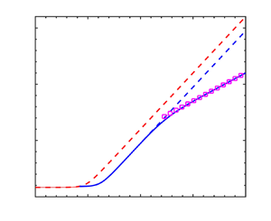
which is a quintic polynomial in  $k^{2}$. Figure 2( $a$) shows the evolution of the real parts of the roots of this quintic polynomial as $\widetilde{Rs\hphantom{.}}$ is increased. With $\widetilde{Rs\hphantom{.}}=0$, the only real positive root is at $k^{2}=1/2$ (the classical case). As $\widetilde{Rs\hphantom{.}}$ increases, the existing mode moves to higher $k^{2}$ and, at a critical value of $\widetilde{Rs\hphantom{.}}$, two equal stationary points appear, which then separate with a further increase in $\widetilde{Rs\hphantom{.}}$; $k^{2}$ remains negative (and thus unphysical) for the other two roots. Figure 2( $b$) plots the oscillatory stability boundary with no approximations, together with the zeroth-order approximation (3.8), and the first-order correction (3.9); the latter is almost indistinguishable from the boundary of the full system. The three stationary points correspond to the three positive roots for $k^{2}$ at $\widetilde{Rs\hphantom{.}}=15$ in figure 2( $a$). Thus the M–C influence is felt for $Rs = O({C_{T}}^{-1})$ by the emergence of two new stationary points in the oscillatory stability boundary. As demonstrated in figure 2, the preferred mode is the continuation of the classical mode, moved to higher wavenumbers.
(a) The real parts of the roots of (3.10) for  $k^{2}$ as a function of $\widetilde{Rs\hphantom{.}}$ for $0 < n \le 1$; blue lines denote real roots, the red line denotes the real part of a conjugate pair; $\sigma =1$, $\tau =0.1$. (b) Oscillatory stability boundary (blue solid line), together with the zeroth-order asymptotic expression (3.8) (purple dashed line) and the first-order correction (3.9) (purple squares); ${C_{T}}=10^{-3}$, ${C_{S}}=0$, $Rs=1.5 \times 10^{4}$ (corresponding to $\widetilde{Rs\hphantom{.}}=15$).

3.2.2. n = 2
In § 3.2.1, we saw how, for  $n=1$, a new pair of stationary points emerges, leading to two minima and one maximum in the $Ra^{(o)}$ versus $k^{2}$ curve, all with $k^{2}=O(1)$. As $Rs$ is increased, (i.e. $n$ increased), these stationary points separate; at $n=2$, they attain distinct asymptotic scalings, with the two minima of $Ra^{(o)}$ having $k^{2} = O({C_{T}})$ and $k^{2} =O( {C_{T}}^{-1} )$, and with the maximum having $k^{2} = O( {C_{T}}^{-1/2})$. This is illustrated clearly in figure 3.
Oscillatory stability boundary versus  $k^{2}$ for ${C_{T}}=10^{-3}$, ${C_{S}}=0$, $Rs=10^{6}$ (i.e. $n=2$) for (a) $\sigma =1$, τ = 0.1; (b) $\sigma =0.05$, $\tau =0.1$. The steady boundary lies at much higher values of $Ra$.
$Ra$.

The value of  $Ra^{(o)}$ for the minimum at $k^{2} = O({C_{T}})$ is readily attained analytically, at least to leading order. Noting that $\beta ^{2} \approx 1$ for small $k^{2}$, the coefficients of (3.4) become, at leading order,
 \begin{equation} c_2 = 4 {C_{T}}^{2}, \quad c_1 ={-} \frac{(1+\sigma)}{\sigma^{2} k^{2}}, \quad c_0 = \frac{(\sigma+\tau) Rs}{\sigma^{2} k^{2}}. \end{equation}
The roots have  $Ra = O( {C_{T}}^{-2})$ and $Ra =O( {C_{T}}^{-3})$, with only the former being admissible ( $\omega ^{2}>0$). Thus, with $k^{2} = O({C_{T}})$,
 \begin{equation} Ra^{(o)} = \frac{(\sigma+\tau)}{(1+\sigma)}Rs + O({C_{T}}^{{-}1}).\end{equation}
We see straightaway that steady modes cannot be preferred when  $n=2$. The wavenumber dependence of $Ra^{(o)}$ has again dropped out at this order, possibly unsurprisingly given the very flat nature of this minimum, as shown in figure 3. If needed, this could be retrieved by retaining the next-order terms. However, numerical calculations suggest that the minimum of $Ra^{(o)}$ at large $k^{2}$ is always the smaller, but that the two minima do become arbitrarily close for small values of $\sigma$ and $\tau$ (cf. figures 3a and 3b). In general, it is not possible to obtain an analytic expression for the minimum value of $Ra^{(o)}$ with $k^{2} =O( {C_{T}}^{-1} )$. However, we can make progress in the case of ${C_{T}} \ll \sigma , \tau \ll 1$, through a distinguished limiting process, in which we first let ${C_{T}} \to 0$ and then let $\sigma$ and $\tau$ become small. To explore the ${C_{T}} \to 0$ limit, we introduce the scalings
 \begin{equation} k^{2} = {C_{T}}^{{-}1} \tilde k^{2}, \quad Ra = {C_{T}}^{{-}2} \widetilde{Ra}, \quad Rs = {C_{T}}^{{-}2} \widetilde{Rs\hphantom{.}}. \end{equation}
The coefficients of expression (3.4) are almost unchanged, except with  $\widetilde{Rs\hphantom{.}}$ replacing $Rs$, etc., and with ${C_{T}}=1$; the substantive difference is that $\beta ^{2} = k^{2}$ at this order. We then let $\sigma$ and $\tau$ become small, with the wavenumber scaled as $\tilde k^{2} = \sigma \hat k^{2}$. The onset of oscillatory instability is then given by
 \begin{equation} \widetilde{Ra}^{(o)} = \frac{(\sigma+\tau)}{(1+\sigma)}( \widetilde{Rs\hphantom{.}} + \sigma (\hat k^{2} - 2 \widetilde{Rs\hphantom{.}} )^{2} + O(\sigma^{2}) ). \end{equation}
Hence  $\widetilde {Ra}^{(o)}$ is minimised when
 \begin{equation} \hat k^{2} = 2 \widetilde{Rs\hphantom{.}}, \quad \text{with } \widetilde{Ra}^{(o)} = \frac{(\sigma+\tau)}{(1+\sigma)} \widetilde{Rs\hphantom{.}} + O(\sigma^{3}).\end{equation}
Thus, to this degree of approximation, one cannot distinguish between the minimum at small  $k^{2}$ (expression (3.12)) and that at large $k^{2}$ (expression (3.15)).
3.2.3. $n>\textit{2}$

As for the case of  $n=2$, there are two minima in $Ra$ as a function of $k^{2}$: the minimum at small wavenumber has $k^{2} =O(C_T^{n-1})$, that at large wavenumber has $k^{2} =O( {C_{T}}^{-n/2})$.
When  $k^{2} =O(C_T^{n-1})$, the frequency equation (3.2), at leading order, becomes
 \begin{equation} 4 {C_{T}} \omega^{4} + \left(1+\frac{1}{\sigma}\right) \omega^{2} - (1-\tau)Rs k^{2} = 0. \end{equation}
There is one admissible root, given by
 \begin{equation} \omega^{2} \approx \frac{\sigma(1-\tau)Rs k^{2}}{(1+\sigma)}, \end{equation}
with the oscillatory stability boundary then given by
 \begin{equation} Ra^{(o)} \approx \frac{(\sigma+\tau)}{(1+\sigma)} Rs. \end{equation}
 For the minimum at large  $k^{2}$, with $k^{2} =O({C_{T}}^{-n/2})$, the frequency equation, at leading order, becomes
 \begin{equation} 2 {C_{T}} \omega^{4} + 2 \tau {C_{T}}Rs \omega^{2} - \tau Rs k^{2} = 0 . \end{equation}
There is one admissible root, given by
 \begin{equation} \omega^{2} \approx \frac{k^{2}}{2 {C_{T}}}. \end{equation}
From the relation  $\omega ^{2} = a_1/a_3$ we then obtain, to leading order,
 \begin{equation} Ra^{(o)} = \frac{1}{2 \tau {C_{T}}} \left( \frac{Rs}{k^{2}}+\tau k^{2} \right).\end{equation}
From (3.21),  $Ra^{(o)}$ is minimised when
 \begin{equation} k^{2} =\left( \frac{Rs}{\tau}\right)^{1/2}, \quad \textrm{with } Ra^{(o)} = \frac{1}{{C_{T}}}\left(\frac{Rs}{\tau} \right)^{1/2}.\end{equation}
 From (3.22), we can see that the minimum at large  $k^{2}$ has $Ra =O({C_{T}}^{-(1+n/2)} )$, whereas from (3.18), that at small $k^{2}$ has $Ra=O( {C_{T}}^{-n})$. Thus for $n>2$ (and in contrast to the case of $n=2$), the two minima have distinct asymptotic scalings: the lower minimum occurs at large $k^{2}$, and is given by (3.22). Furthermore, since the onset of steady convection is given by $Ra^{(s)} \approx Rs/\tau = O({C_{T}}^{-n})$, oscillatory modes are always preferred for $n>2$.
3.2.4. Overall stability boundary
It is important to put together the above ideas in order to determine the critical Rayleigh number and the associated critical wavenumber for a wide range of  $Rs$ (i.e. for a range of $n$). Figure 4(a) shows $Ra_c$ for the range $10^{-5} \le Rs \le 10^{15}$ (corresponding to $-5/3 \le n \le 5$) for fixed values of ${C_{T}}=10^{-3}$, $\sigma =1$, $\tau = 0.1$, together with the asymptotic results for $n>2$. Figure 4(b) shows $k_c^{2}$ at the onset of instability. For small enough $Rs$, the onset is always steady, with $k_c^{2}=1/2$. As $Rs$ is increased, the preferred mode becomes oscillatory, initially with little change in the wavenumber of the critical mode. However, for $n \gtrsim 1$, the critical wavenumber increases with increasing $Rs$: for the $n=2$ regime, $Ra_c$ and $k_c^{2}$ both depend linearly on $Rs$ (e.g. expression (3.15) for small $\sigma$ and $\tau$), whereas for $n>2$, $Ra_c$ and $k_c^{2}$ both vary as $Rs^{1/2}$ (expression (3.22)). Also shown in figure 4(a) is the onset of oscillatory instability for the classical problem. In terms of the critical Rayleigh number (but, as noted above, not the preferred wavenumber), it can be seen that the M–C effect only comes into play strongly for $n \gtrsim 2$, where it leads to a clear enhanced destabilisation of the oscillatory modes.
Plots of (a)  $Ra_c$ and (b) $k_c^{2}$ as a function of $Rs$ for ${C_{T}}=10^{-3}$, ${C_{S}}=0$, $\sigma =1$, $\tau =0.1$. The onset of instability is shown as a red solid line if steady and a blue solid line if oscillatory. The red dashed line shows the continuation of the steady line once it is no longer preferred. The blue dashed line denotes the onset of oscillatory instability for the classical problem. The purple squares denote the asymptotic $n>2$ results (3.22).

3.3. Third quadrant: $Ra<0$, $Rs<0$


3.3.1. $n \le \textit{2}$

As discussed in § 2.3, for classical double-diffusive convection the onset of instability in the third quadrant is always via a steady bifurcation (salt fingers). Therefore, in comparison with the first quadrant (for which the classical problem has an oscillatory instability), larger values of  $|Rs|$ are needed before there are substantive variations from classical double-diffusive convection: M–C effects are not felt until $n=2$ (i.e. $Rs=O({C_{T}}^{-2})$). For $n=2$, the minimum in the $Ra^{(o)}$ curve as a function of $k^{2}$ is located in the regime of $k^{2} = O( {C_{T}}^{-1/2})$ (which in the first quadrant is the location of a local maximum). The behaviour in this regime is captured by the orderings $k^{2} \sim \beta ^{2} =O({C_{T}}^{-1/2})$, and $Ra, Rs =O({C_{T}}^{-2})$; we write $k^{2}= {C_{T}}^{-1/2} \tilde k^{2}$, $Ra = {C_{T}}^{-2} \widetilde {Ra}$, etc.
At leading order, (3.4), governing the onset of oscillatory convection, becomes
 \begin{equation} 4 \widetilde{Ra}^{2} -\frac{1}{\sigma^{2}} ( (1+\sigma) + 4\sigma (2\sigma + \tau) \widetilde{Rs\hphantom{.}} ) \widetilde{Ra} + \frac{4(\sigma+\tau)}{\sigma} \widetilde{Rs\hphantom{.}}^{2} + \frac{(\sigma+\tau)}{\sigma^{2}} \widetilde{Rs\hphantom{.}} = 0. \end{equation}
To this order there is no wavenumber dependence of  $\widetilde {Ra}$ and thus to determine the dependence on $k^{2}$, we need to retain terms of the next order; we thus write $\widetilde {Ra}= \widetilde {Ra}_0 + {C_{T}}^{1/2} \widetilde {Ra}_1$. The leading-order terms determine $\widetilde {Ra}_0$ via (3.23); $\widetilde {Ra}_1$ is determined at the next order through the expression
 \begin{equation} F \widetilde{Ra}_1 = \left( A \tilde k^{2} + \frac{B}{\tilde k^{2}}\right),\end{equation}
where
 $$\begin{gather} F = 8(\widetilde{Rs\hphantom{.}}-\widetilde{Ra}_0) + \frac{4 \tau}{\sigma}\widetilde{Rs\hphantom{.}} + \left( \frac{1+\sigma}{\sigma^{2}}\right), \end{gather}$$
 $$\begin{gather}A = 8 \tau \widetilde{Ra}_0^{2} - \frac{8\tau(\sigma + \tau)}{\sigma} \widetilde{Ra}_0 \widetilde{Rs\hphantom{.}} - \frac{2(\tau + \sigma \tau + \sigma^{2})}{\sigma^{2}}\widetilde{Ra}_0 + \frac{2 (\sigma+\tau-2)(\sigma+\tau)}{\sigma^{2}}\widetilde{Rs\hphantom{.}}, \end{gather}$$
 $$\begin{gather}B ={-} \frac{(1+\sigma)}{\sigma^{2}} \widetilde{Ra}_0 + \frac{(\sigma+\tau)}{\sigma^{2}}\widetilde{Rs\hphantom{.}}. \end{gather}$$
If  $F$,
$F$,  $A$ and $B$ are of the same sign, then $\widetilde {Ra}_1$ is minimised when
 \begin{equation} \tilde k^{2} = \left( \frac{B}{A}\right)^{1/2}.\end{equation}
 Figure 5 shows the stability boundaries for oscillatory and steady modes as functions of  $k^{2}$, together with the associated values of $\omega ^{2}$; also shown are the asymptotic results (3.23) and (3.24). It can be seen that oscillatory instability occurs within a closed loop in the $(Ra,k^{2})$ plane. As $|Rs|$ decreases (i.e. $Rs$ becomes less negative), the loop shrinks, eventually disappearing altogether; equivalently, and maybe what is a more natural way of thinking, in terms of an experiment, the loop appears at a critical value of $Rs$ as $|Rs|$ is increased. An important feature is that this spontaneous appearance may occur either above or below the steady branch. To determine the least negative value of $Rs$ for which oscillations are possible thus requires determination of the critical value of $Rs$ for which the loop first appears, calculation of $Ra$ at that value, and a comparison with the value of $Ra$ on the steady branch at the same value of $Rs$.
$Rs$.
(a) Stability boundaries versus  $k^{2}$ for ${C_{T}}=10^{-4}$, ${C_{S}}=0$, $Rs=-10^{9}$, $\sigma =0.2$, $\tau =0.5$. The loop shown in brown and blue is the oscillatory stability boundary, with the two colours representing the two roots of the quadratic for $Ra$; the red line shows the steady boundary. The green dashed line shows the first-order asymptotic result (3.23); the purple dashed line includes the next-order correction (3.24). (b) Corresponding values of $\omega^2$ on the oscillatory stability boundary.

The loop of oscillatory instability appears when the two roots of (3.23) coincide. After a little algebra, it can be shown that the critical value of  $\widetilde{Rs\hphantom{.}}$ ( $\widetilde{Rs\hphantom{.}}_\ell$, say) is then given by
 \begin{equation} \frac{1}{\sigma} = 4 \tau |\widetilde{Rs\hphantom{.}}_\ell| -4 |\widetilde{Rs\hphantom{.}}_\ell|^{1/2}(1-\tau)^{1/2}-1. \end{equation}
For comparison, we must also calculate the values of  $\widetilde{Rs\hphantom{.}}$ at which the stability boundaries for the steady and oscillatory modes intersect ( $\widetilde{Rs\hphantom{.}}_{so}$, say). At leading order, the steady boundary (2.21) is approximated by $\widetilde {Ra} = \widetilde{Rs\hphantom{.}}/\tau$. Substituting into (3.23), the leading-order expression for the oscillatory stability boundary, gives
 \begin{equation} \widetilde{Rs\hphantom{.}}_{so} = \frac{\tau (1 + \sigma + \tau)}{4\sigma (\sigma-\sigma\tau-\tau^{2})}.\end{equation}
The comparison to be made is between  $\widetilde {Ra}$ evaluated at $\widetilde{Rs\hphantom{.}}_\ell$, when the loop first appears, and $\widetilde{Rs\hphantom{.}}_\ell /\tau$, which is the value of $\widetilde {Ra}$ on the steady branch. If $\widetilde {Ra}(\widetilde{Rs\hphantom{.}}_\ell ) < \widetilde{Rs\hphantom{.}}_\ell /\tau$ (both negative recall), then the loop of oscillations appears beneath the steady branch (i.e. at higher $|\widetilde {Ra}|$); the critical value of $\widetilde{Rs\hphantom{.}}$ for the onset of oscillations is then $\widetilde{Rs\hphantom{.}}_\ell$. If, on the other hand, $\widetilde {Ra}(\widetilde{Rs\hphantom{.}}_\ell ) > \widetilde{Rs\hphantom{.}}_\ell /\tau$, then the loop of oscillations appears above the steady branch (i.e. at lower $|\widetilde {Ra}|$); the critical value of $\widetilde{Rs\hphantom{.}}$ for the onset of oscillations is then $\widetilde{Rs\hphantom{.}}_{so}$. It can be shown that $\widetilde{Rs\hphantom{.}}_\ell = \widetilde{Rs\hphantom{.}}_{so}$ when
 \begin{equation} \sigma = \frac{1}{2} \left( \sqrt{\frac{1+3 \tau}{1-\tau}} - (1+2 \tau ) \right).\end{equation}
 Figure 6(a) shows the critical value of  $\widetilde{Rs\hphantom{.}}$ as a function of $\tau$ for the case of $\sigma =0.3$. For this value of $\sigma$, the critical value of $\tau$ distinguishing the two regimes, given by expression (3.29), is $\tau = 0.649$. We note also, from (3.28), that $\widetilde{Rs\hphantom{.}}_{so} \to - \infty$ as $(\sigma - \sigma \tau - \tau ^{2}) \to 0$; thus oscillations can be preferred in the third quadrant only if the following inequality is satisfied:
 \begin{equation} \sigma < \frac{\tau^{2}}{1-\tau} ;\end{equation}
for  $\sigma =0.3$, this gives the lower bound of $\tau = 0.418$. Figure 6(b) shows the corresponding critical value of $\tilde k^{2}$, as determined by expression (3.26), at the onset of oscillatory instability.
(a) Critical value of  $\widetilde{Rs\hphantom{.}}$ for the onset of oscillatory instability with $n=2$ as a function of $\tau$ for $\sigma = 0.3$ (with ${C_{S}}=0$). On the dashed line, oscillatory instability first occurs when the oscillatory and steady branches coincide. On the solid line, oscillatory instability first occurs through the appearance of a loop beneath the steady boundary. (b) The value of $\tilde k^{2}$ at the onset of oscillatory instability.

3.3.2. $n>\textit{2}$

In the third quadrant, the oscillatory mode remains minimised when  $k^{2} = O( {C_{T}}^{-1/2})$ for $n>2$. This property thus allows us readily to determine the oscillatory stability boundary from (3.23) (valid for $n=2$) simply by considering the case of $|\widetilde{Rs\hphantom{.}}|, |\widetilde {Ra}| \gg 1$. In this limit, (3.23) factorises to give the two leading-order solutions
 \begin{equation} \widetilde{Ra} = \widetilde{Rs\hphantom{.}}, \quad \widetilde{Ra} = \frac{(\sigma+\tau)}{\sigma}\widetilde{Rs\hphantom{.}}. \end{equation}
Recall that at leading order, the steady branch is given by  $\widetilde {Ra} = \widetilde{Rs\hphantom{.}}/\tau$. Thus, since $\tau <1$, the root $\widetilde {Ra} = \widetilde{Rs\hphantom{.}}$ always lies above the steady branch and hence is of no physical relevance. However, the root $\widetilde {Ra} = (\sigma +\tau ) \widetilde{Rs\hphantom{.}}/\sigma$ lies below the steady branch provided that inequality (3.30) holds; i.e. the same condition applies for $n>2$ as for $n=2$.Since there is cancellation at leading order in expression (3.25b) for the coefficient $A$, in order to determine the preferred value of the wavenumber at onset it is necessary to include the first-order correction to $\widetilde {Ra}$, which gives
 \begin{equation} \widetilde{Ra} = \frac{(\sigma + \tau)}{\sigma}\widetilde{Rs\hphantom{.}} + \left(\frac{\sigma+\tau}{4 \sigma^{2} \tau} \right) {C_{T}}^{n-2}. \end{equation}
From (3.26), having made use of (3.25) and (3.32), we determine the critical value of  $\tilde k^{2}$ at the onset of instability as
 \begin{equation} \tilde k^{2}= \left( \frac{1}{2\sigma}\right)^{1/2}.\end{equation}
3.3.3. Overall stability boundary
Figure 7(a) shows the critical Rayleigh number  $Ra_c$ for a wide range of $Rs$ ( $-5 \ge Rs \ge -10^{15}$, equivalent to $O(1) \le n \le 5$), for fixed values of ${C_{T}}=10^{-3}$, $\tau =0.5$, $\sigma =0.3$. For small enough $|Rs|$, the preferred mode at onset is always steady, with $k^{2}=1/2$, as shown in figure 7(b). For $n>2$, since inequality (3.30) is satisfied with this choice of parameters, oscillatory modes are preferred; figure 7(b) confirms that the critical wavenumber for the oscillatory modes has $k^{2} = O( {C_{T}}^{-1/2})$ for all $n>2$. If there is a transition between steady and oscillatory modes, as here, it occurs when $n \approx 2$; for the parameter values in figure 7, the transition occurs at $Rs=-7.9 \times 10^{6}$. For both the steady and oscillatory branches, $Ra_c$ varies linearly with $Rs$; the offset between the two is made clear in the inset, which plots $Ra_c/|Rs|$ against $Rs$.
$Rs$.
Plots of (a)  $Ra_c$ and (b) $k_c^{2}$ as a function of $Rs$ ( $-5 \ge Rs \ge -10^{15}$) for ${C_{T}}=10^{-3}$, ${C_{S}}=0$, $\sigma =0.3$, $\tau =0.5$. The onset of instability is shown as a red solid line if steady and a blue solid line if oscillatory. The red dashed line shows the continuation of the steady line once it is no longer preferred. The inset plots $Ra_c$ versus $Ra_c/|Rs|$ in order to distinguish more clearly the steady and oscillatory branches.

4. The case of ${C_{T}}=0$

4.1. Stability boundaries
As for the case of  ${C_{S}}=0$, the coefficient $a_5$ defined by (2.18a) vanishes; the dispersion relation (2.17) reduces to a quartic equation with coefficients
 $$\begin{align} a_4 &= 2 {C_{S}} \frac{\beta^{2}}{\sigma}, \end{align}$$
 $$\begin{align}a_3 &= 2 {C_{S}} \beta^{4} \left( 1 + \frac{1}{\sigma}\right) + \frac{\beta^{2}}{\sigma}, \end{align}$$
 $$\begin{align}a_2 &= 2 {C_{S}} \beta^{6} + \beta^{4} \left( 1 + \frac{1+\tau}{\sigma}\right) + 2 {C_{S}} (Rs-Ra)k^{2}, \end{align}$$
 $$\begin{align}a_1 &= \left(1 + \tau + \frac{\tau}{\sigma}\right) \beta^{6} - Ra k^{2} + Rs k^{2} (1 + 2 {C_{S}} \beta^{2} ), \end{align}$$
 $$\begin{align}a_0 &= \tau \beta^{8} - \tau Ra k^{2} \beta ^{2} + Rs k^{2} \beta^{2}. \end{align}$$
Again, for an oscillatory root we have the conditions
 \begin{equation} a_4 \omega^{4} - a_2 \omega^{2} +a_0=0, \quad a_3 \omega^{2} - a_1 =0. \end{equation}
Eliminating  $Ra$ gives the following quadratic equation for $\omega ^{2}$:
 \begin{equation} b_4 \omega^{4} + b_2 \omega^{2} + b_0 = 0,\end{equation}
where
 $$\begin{align} b_4 &=4 {C_{S}}^{2} \beta^{2} , \end{align}$$
 $$\begin{align}b_2 &= \beta^{2} - 4 {C_{S}}^{2} Q k^{2} - 4 \tau {C_{S}} \beta^{4} , \end{align}$$
 $$\begin{align}b_0 &= \tau^{2} \beta^{6} - Q k^{2} (1-\tau) + 2 \tau {C_{S}}Q \beta^{2} k^{2}, \end{align}$$
where  $Q=\sigma Rs/(1+\sigma )$.
Conversely, we could eliminate  $\omega ^{2}$ to obtain the following quadratic expression for $Ra$ on the oscillatory boundary (provided that $\omega ^{2}>0$):
 \begin{equation} c_2 Ra^{2} + c_1 Ra + c_0 =0,\end{equation}
where
 \begin{align} c_2 &= 4 \sigma^{2} (1+\sigma) {C_{S}}^{2}, \end{align}
 \begin{align} c_1 &={-} \left(8 \sigma^{2} (1+\sigma) {C_{S}}^{3} R_s \beta^{2} + 8 \sigma^{2} (1+\sigma) {C_{S}}^{2} \frac{\beta^{6}}{k^{2}} + 4 \sigma^{2} (1+2\sigma) {C_{S}}^{2} R_s \right. \nonumber\\ & \quad+ \left. 2\sigma(1+\sigma)(1+\sigma-2 \tau) {C_{S}} \frac{\beta^{4}}{k^{2}} + \sigma(1+\sigma) \frac{\beta^{2}}{k^{2}} \right), \end{align}
 \begin{align} c_0&= 8 {C_{S}}^{3} \sigma^{2} R_s \beta^{2} \left((1+\sigma) \frac{\beta^{6}}{k^{2}} + \sigma R_s\right) \nonumber\\ &\quad+ 4 {C_{S}}^{2} \left( \sigma^{3} \left( \frac{\beta^{6}}{k^{2}} + R_s \right)^{2} + \sigma^{2} (1+\tau+\sigma \tau)R_s \frac{\beta^{6}}{k^{2}} + \sigma^{2} \frac{\beta^{12}}{k^{4}} \right) \nonumber\\ & \quad+ 2 {C_{S}} \frac{\beta^{4}}{k^{2}} \left( (\sigma^{2} (1+\sigma)+ \sigma \tau) R_s + (1+\sigma)(\tau (1+\sigma^{2})+\sigma(1+\sigma)) \frac{\beta^{6}}{k^{2}} \right) \nonumber\\ & \quad+ (1+\sigma)(1+\tau)(\sigma+\tau) \frac{\beta^{8}}{k^{4}} + \sigma (\sigma+\tau) R_s \frac{\beta^{2}}{k^{2}}. \end{align}
4.2. First quadrant: $Ra>0$, $Rs>0$


4.2.1. $n \le \textit{1}$

We first recall that once  $Rs$ is such that inequality (2.24) is satisfied then oscillatory modes are preferred. In an analogous fashion to the case of ${C_{S}}=0$, we may investigate the changes from the classical problem when $n=1$. We consider the regime ${C_{S}} \ll 1$, $Rs={C_{S}}^{-1}\widetilde{Rs\hphantom{.}}$, $Ra={C_{S}}^{-1}\widetilde {Ra}$, with $k^{2}=O(1)$, and write $\widetilde {Ra} = \widetilde {Ra}_0 + {C_{S}} \widetilde {Ra}_1$. On substitution into (4.5), the leading-order terms give
 \begin{equation} \widetilde{Ra}_0=\frac{(\sigma+\tau)}{(1+\sigma)} \widetilde{Rs\hphantom{.}}.\end{equation}
The wavenumber dependence appears at the next order, where  $\widetilde {Ra}_1$ is given by
 \begin{equation} \widetilde{Ra}_1 ={-}\frac{4 \sigma \tau(1-\tau)}{(1+\sigma)^{2}} \widetilde{Rs\hphantom{.}}^{2} \frac{k^{2}}{\beta^{2}} + \frac{2\tau(\sigma+2\tau)}{(1+\sigma)} \widetilde{Rs\hphantom{.}} \beta^{2} + \frac{(1+\tau)(\sigma+\tau)}{\sigma} \frac{\beta^{6}}{k^{2}}.\end{equation}
Stationary points ( $\textrm {d} \widetilde {Ra}_1/\textrm {d} k^{2} =0$) are therefore given by the expression
 \begin{align} \frac{4 \sigma \tau(1-\tau)}{(1+\sigma)^{2} (1+k^{2})^{2}} \widetilde{Rs\hphantom{.}}^{2} - \frac{2 \tau (\sigma+2 \tau)}{(1+\sigma)} \widetilde{Rs\hphantom{.}} - \frac{(1+\tau)(\sigma+\tau)}{\sigma} (2k^{2}-1)\frac{(1+k^{2})^{2}}{k^{4}} =0,\end{align}
which is a quintic polynomial in  $k^{2}$. Figure 8(a) shows the evolution of the real parts of the roots of this polynomial as $\widetilde{Rs\hphantom{.}}$ is increased. By contrast with the case of ${C_{S}}=0$ (cf. figure 2 $a$), no new positive stationary points arise. As $\widetilde{Rs\hphantom{.}}$ is increased, and contrary to the behaviour in the first quadrant when ${C_{S}}=0$ (see § 3.2.1), the minimum at $k^{2}=1/2$ of the classical problem first moves to slightly lower wavenumbers, for all $\sigma$ and $\tau < 1$, before then moving gradually to higher wavenumbers. The smallest value of $k_c^{2}$, taken over $\widetilde{Rs\hphantom{.}}$, is given by the positive root of the quadratic equation
 \begin{equation} \frac{\tau(\sigma+2\tau)^{2}}{4(1-\tau^{2})(\sigma+\tau)} k_c^{4} + 2 k_c^{2} -1 =0. \end{equation}
Figure 8(b) plots the oscillatory stability boundary, together with the zeroth-order approximation (4.7), and the first-order correction (4.8); the latter is almost indistinguishable from the boundary of the full system.
(a) The real parts of the roots of (4.9) for  $k^{2}$ as a function of $\widetilde{Rs\hphantom{.}}$ for the $n=1$ regime; the blue line denotes a real root, the red lines denote the real part of a conjugate pair; $\sigma =1$, $\tau =0.5$. (b) Oscillatory stability boundary (blue solid line) for ${C_{S}}=10^{-3}$, ${C_{T}}=0$, $Rs=2 \times 10^{4}$ (corresponding to $\widetilde{Rs\hphantom{.}} = {C_{S}}Rs = 20$), together with the zeroth-order asymptotic expression (4.7) (purple dashed line) and the first-order correction (4.8) (purple squares).

4.2.2. $n=\textit{2}$

In the first quadrant, the critical  $Ra$ for oscillatory modes is minimised when $k^{2} = O( {C_{S}}^{-1/2} )$. At leading order, the coefficients of (4.5) become
 $$\begin{align} c_2 &= 4 \sigma^{2} (1+\sigma) {C_{S}}^{2}, \end{align}$$
 $$\begin{align}c_1 &={-} (4 \sigma^{2} (1+2\sigma) {C_{S}}^{2} Rs + \sigma(1+\sigma) ), \end{align}$$
 $$\begin{align}c_0 &= 4 {C_{S}}^{2} \sigma^{3} Rs^{2} + \sigma (\sigma+\tau) Rs . \end{align}$$
In terms of the scaled variables defined by  $Ra = {C_{S}}^{-2}\widetilde {Ra}$, $Rs = {C_{S}}^{-2}\widetilde{Rs\hphantom{.}}$, this gives the following quadratic equation:
 \begin{equation} 4 \sigma (1+\sigma) \widetilde{Ra}^{2} - (4 \sigma (1+2\sigma) \widetilde{Rs\hphantom{.}} + (1+\sigma) ) \widetilde{Ra} + 4 \sigma^{2} \widetilde{Rs\hphantom{.}}^{2} + (\sigma+\tau) \widetilde{Rs\hphantom{.}} = 0.\end{equation}
It may be verified that in this regime, oscillations are favoured for all values of the parameters. To see this, we note that the marginal curve for oscillations (4.12) is a hyperbola passing through the origin, which can be written in the form
 \begin{align} ((1+\sigma)\widetilde{Ra}-\sigma\widetilde{Rs\hphantom{.}}-e)(\widetilde{Ra}-\widetilde{Rs\hphantom{.}}-f)=ef, \quad \mbox{where } e=\frac{\tau(1+\sigma)}{4\sigma},~~f=\frac{(1-\tau)}{4\sigma} . \end{align}
This hyperbola intersects the line  $\widetilde{Rs\hphantom{.}}=0$ at $\widetilde {Ra}=0,\widetilde {Ra}=1/4\sigma$. Thus it is the lower branch of the hyperbola that passes through the origin, and the gradient along this branch decreases monotonically along the branch from $(\sigma +\tau )/(1+\sigma )$ to $\sigma /(1+\sigma )$; hence the gradient is always less than $1/\tau$, and oscillations are therefore always preferred in the first quadrant when $Rs=O({C_{S}}^{-n}), n\ge 2$.
As in § 3.3, we must take the analysis to the next order to determine the wavenumber dependence of the critical Rayleigh number; we thus write  $\widetilde {Ra}= \widetilde {Ra}_0 + {C_{S}}^{1/2} \widetilde {Ra}_1$. The leading-order terms determine $\widetilde {Ra}_0$ via (4.12); $\widetilde {Ra}_1$ is determined at the next order through the expression
 \begin{equation} F \widetilde{Ra}_1 = \left( A \tilde k^{2} + \frac{B}{\tilde k^{2}}\right),\end{equation}
where
 \begin{gather} \hspace{30pt}F = 4 \sigma^{2} (1+2 \sigma)\widetilde{Rs\hphantom{.}} + \sigma (1+\sigma) - 8 \sigma^{2} (1+\sigma) \widetilde{Ra}_0 , \end{gather}
 \begin{gather} A = 8 \sigma^{3} \widetilde{Rs\hphantom{.}}^{2} - 8 \sigma^{2} (1+\sigma)\widetilde{Rs\hphantom{.}} \widetilde{Ra}_0 + 2 ( \sigma^{2}(1+\sigma)+\sigma \tau )\widetilde{Rs\hphantom{.}}\notag\\ -2 \sigma(1+\sigma)(1+\sigma-2\tau)\widetilde{Ra}_0, \end{gather}
 \begin{gather} \hspace{30pt}B = \sigma (\sigma+\tau) \widetilde{Rs\hphantom{.}} - \sigma (1+\sigma) \widetilde{Ra}_0. \end{gather}
If  $F$,
$F$,  $A$ and $B$ are of the same sign, then $\widetilde {Ra}_1$ is minimised when
 \begin{equation} \tilde k^{2} = \left( \frac{B}{A}\right)^{1/2}.\end{equation}
Figure 9 shows  $Ra^{(o)}$ as a function of $k^{2}$, together with the asymptotic results (4.12) and (4.14), for ${C_{S}}=10^{-4}$ and ${C_{S}}=10^{-8}$.
The blue lines show the oscillatory stability boundary  $Ra^{(o)}$ versus $k^{2}$ with $\sigma =1$, $\tau =0.1$, ${C_{T}}=0$; (a) ${C_{S}}=10^{-4}$, $Rs=10^{8}$; (b) ${C_{S}}=10^{-8}$, $Rs=10^{16}$. The purple dashed lines show the leading-order asymptotic result (4.12); the purple squares include the first-order correction given by (4.14). At the smaller value of ${C_{S}}$, the numerical results for the full system and the first-order asymptotic results are essentially indistinguishable.

4.2.3. $n>\textit{2}$

As in the third quadrant with  ${C_{S}}=0$ (§ 3.3.2), for $n>2$ the oscillatory mode remains minimised when $k^{2} = O( {C_{S}}^{-1/2})$. The ensuing analysis to determine the critical wavenumber is thus entirely analogous, with the oscillatory stability boundary determined from (4.12) (valid for $n=2$) by considering the case of $|\widetilde{Rs\hphantom{.}}|, |\widetilde {Ra}| \gg 1$. In this limit, (4.12) factorises to give the following two leading-order solutions:
 \begin{equation} \widetilde{Ra} = \widetilde{Rs\hphantom{.}}, \quad \widetilde{Ra} = \frac{\sigma}{(1+\sigma)}\widetilde{Rs\hphantom{.}},\end{equation}
where the latter is the critical value for the onset of oscillatory instability (which is always the preferred mode). To determine the critical value of the wavenumber at the onset of oscillatory instability, it is again necessary to include the first-order correction to  $\widetilde {Ra}$, which gives
 \begin{equation} \widetilde{Ra} = \frac{\sigma}{(1+\sigma)}\widetilde{Rs\hphantom{.}} + \left( \frac{\tau}{4 \sigma}\right) {C_{S}}^{n-2}. \end{equation}
From (4.16), having made use of (4.15) and (4.18), we can determine the critical value of  $\tilde k^{2}$ at the onset of instability as
 \begin{equation} \tilde k^{2}= \left( \frac{1}{2\sigma}\right)^{1/2}.\end{equation}
The onset of instability in the first quadrant for  ${C_{T}}=0$ is related to that in the third quadrant for ${C_{S}}=0$. The leading-order expressions (3.32) and (4.18) are connected through the transformation (2.19). The critical wavenumbers are identical in the two cases, although this is not readily shown via the transformation (2.19) – the symmetry is lost since both analyses involve perturbations in $Ra$ but not in $Rs$.
$Rs$.
4.2.4. Overall stability boundary
Figure 10 shows  $Ra_c$ and $k_c^{2}$ for $10^{-5} \le Rs \le 10^{15}$ with ${C_{T}}=10^{-3}$, $\sigma =1$, $\tau =0.5$. The steady mode, with $k_c^{2}=1/2$, gives way to the oscillatory mode when $Rs=O(1)$. When it first becomes dominant, the oscillatory mode also has $k_c^{2}=1/2$. As $Rs$ is increased,in the $n=1$ regime, $k_c^{2}$ decreases slightly, as explained in § 4.2.1, before increasing sharply in the $n=2$ regime. For $n\ge 2$, $k_c^{2}=O ({C_{S}}^{-1/2})$, with the precise asymptotic value (4.19) for $n>2$. Also shown in figure 10(a) is the boundary for the onset of oscillatory motion for the classical problem. In terms of $Ra_c$, it can be seen that the M–C effect comes into play for $n \gtrsim 2$, although, since $Ra_c$ depends linearly on $Rs$ for both these boundaries, the difference is small on a logarithmic scale; it is made clearer in the inset, which brings out the difference in the multiplicative factors in (2.23) and (4.17). It is though worth reiterating that the difference in the spatial structure of the preferred modes between the case of ${C_{S}}=0$ and that of ${C_{S}} \ll 1$ is significant; as illustrated in figure 10(b), the former has $k_c^{2}=1/2$, the latter $k_c^{2}=O ({C_{S}}^{-1/2})$.
Plots of (a)  $Ra_c$ and (b) $k_c^{2}$ as a function of $Rs$ ( $10^{-5} \le Rs \le 10^{15}$) for ${C_{T}}=10^{-3}$, ${C_{S}}=0$, $\sigma =1$, $\tau =0.5$. The onset of instability is shown as a red solid line if steady and a blue solid line if oscillatory. The red dashed line shows the continuation of the steady line once it is no longer preferred. The blue dashed line denotes the onset of oscillatory instability for the classical problem. The inset plots $Ra_c$ versus $Ra_c/Rs$ in order to distinguish more clearly the steady and oscillatory branches; here the range of $Rs$ starts at $10^{0.5}$.

4.3. Third quadrant: $Ra<0$, $Rs<0$


4.3.1. $n=\textit{2}$

As for the third quadrant in the case of  ${C_{S}}=0$, discussed in § 3.3, steady convection in the form of salt fingers is always preferred for $n<2$. For $n=2$, oscillatory solutions arise for a range of wavenumbers lying between two Takens–Bogdanov points, defined as where the steady and oscillatory branches coincide, with the oscillatory branch having two zero frequencies. At such points, the coefficients $a_0$ and $a_1$ of the dispersion relation (given by expressions (4.1d,e)) must both vanish. For large $|Rs|$ ( $n \ge 2$), simultaneous solution of the equations $a_0=0$ and $a_1=0$ requires large $k^{2}$. Thus, making only the approximation that $\beta ^{2} \approx k^{2}$, eliminating $Ra$ gives the following condition for Takens–Bogdanov points:
 \begin{equation} \tau^{2} \left( 1+\frac{1}{\sigma}\right) k^{4} + 2 \tau {C_{S}}Rs k^{2} - Rs (1-\tau)=0. \end{equation}
Thus when  $Rs=O({C_{T}}^{-2})$, $k^{2}$ must be $O({C_{S}}^{-1})$. The two Takens–Bogdanov points coincide – marking the first appearance of oscillatory solutions – when there are repeated roots for $k^{2}$ in (4.20); this occurs when
 \begin{equation} Rs = Rs_{{TB}} ={-} \frac{(1-\tau)}{{C_{S}}^{2}} \left(1+\frac{1}{\sigma}\right), \quad \text{with } k^{2} = \left( \frac{1}{\tau}-1\right){C_{S}}^{{-}1}. \end{equation}
When  $Rs = Rs_{{TB}}$, $Ra$ is given by
 \begin{equation} Ra = Ra_{{TB}} = \frac{(1-\tau)(\sigma - \tau - 2 \sigma \tau)}{\sigma \tau^{2}} {C_{S}}^{{-}2}. \end{equation}
Thus, oscillatory solutions first appear in the third quadrant if  $\tau > \sigma /(1+2\sigma )$; otherwise they first appear in the second quadrant. When oscillatory solutions first appear, at $Rs = Rs_{{TB}}$, they are not favoured, even when $(Rs_{{TB}},Ra_{{TB}})$ lies in the third quadrant. As $Rs$ is decreased below $Rs_{{TB}}$, the extent of $k^{2}$ for which oscillatory solutions exist increases, but initially without oscillations being preferred, as shown in figure 11(a). However, as $Rs$ is decreased further – but still within the $n=2$ regime – the minimum of the oscillatory loop lies below the minimum of the steady branch and oscillations are then favoured; this is the situation shown in figure 11(b). Analytically, it is not possible to pin down the transition values of $Rs$ and $k^{2}$ precisely since, save for the approximation $\beta ^{2} \approx k^{2}$, no additional simplification is possible of the terms in (4.5), which are all of the same order.
Critical  $Ra$ for the steady mode (red line) and oscillatory mode (blue line) for $\sigma =1$, $\tau =0.2$, ${C_{S}}=10^{-3}$, ${C_{T}}=0$ with (a) $Rs=-2.5 \times 10^{6}$ and (b) $Rs=-6.5 \times 10^{6}$. In (a), steady convection is favoured, with the preferred mode having $k^{2}=0.5$; in (b), oscillatory convection is favoured, with the preferred mode having $k^{2}=5954$.

4.3.2. $n > \textit{2}$

For  $n>2$, expression (4.20) for the Takens–Bogdanov points, being based only on the condition $k^{2} \gg 1$, is still valid, with roots
 \begin{equation} k^{2} \approx \frac{(1-\tau) {C_{S}}^{{-}1}}{2 \tau}, \quad k^{2} \approx \frac{- 2 \sigma {C_{S}}Rs}{\tau ( 1+ \sigma )} = \frac{- 2 {C_{S}}Q }{\tau}. \end{equation}
Thus, in comparison with the case of  $n=2$, the arc of oscillatory instability is extended; the lower value of $k^{2}$ remains $O({C_{S}}^{-1})$, with the upper value now $O({C_{S}}^{1-n})$. The minimum of the oscillatory stability boundary is captured in the same scaling for $k^{2}$ as the upper Takens–Bogdanov point. Thus, with $k^{2} \sim {C_{S}}^{1-n}$, the frequency equation (4.3) becomes, at leading order,
 \begin{equation} 4{C_{S}}^{2} \omega^{4} - 4 ( {C_{S}}^{2} Q + \tau {C_{S}}k^{2} ) \omega^{2} + ( 2 \tau {C_{S}}Q k^{2} + \tau^{2} k^{4} ) = 0,\end{equation}
which factorises as
 \begin{equation} (2 {C_{S}} \omega^{2} - \tau k^{2})(2 {C_{S}} \omega^{2} - 2 {C_{S}}Q - \tau k^{2} ) =0. \end{equation}
The relevant root for the stability boundary is given by  $\omega ^{2} = \tau k^{2}/2 {C_{S}}$, which is always admissible. The oscillatory stability boundary is then determined from the leading-order terms in expression (2.22) to be
 \begin{equation} Ra^{(o)} = k^{4} +2 {C_{S}}Rs k^{2}, \end{equation}
which, after minimisation over  $k^{2}$, gives
 \begin{equation} Ra_c^{(o)} ={-} {C_{S}}^{2} Rs^{2}, \text{ obtained when } k^{2} ={-}{C_{S}}Rs. \end{equation}
Since the onset of steady convection occurs when  $Ra = Rs/\tau = O( {C_{S}}^{-n})$, then, for $n>2$, oscillatory convection, with onset given by (4.27), is always preferred.
4.3.3. Overall stability boundary
Figure 12 shows  $Ra_c$ and $k_c^{2}$ for $-10^{15} \le Rs \le -4$, for fixed values of ${C_{S}}=10^{-3}$, ${C_{T}}=0$, $\tau =0.5$, $\sigma =0.3$. For small enough $|Rs|$, the preferred mode at onset is always steady, whereas for $n \gtrsim 2$, oscillatory modes are preferred. There is an abrupt change in scale of the preferred mode, from $k_c^{2}=1/2$ to $k_c^{2} = O( {C_{S}}^{-1})$ in the $n=2$ regime. For $n >2$, oscillatory modes are vastly preferred, with $Ra_c$ scaling as $Rs^{2}$; $k_c^{2}$ increases linearly with $Rs$.
$Rs$.
Plots of (a)  $Ra_c$ and (b) $k_c^{2}$ as a function of $Rs$ ( $-10^{15} \le Rs \le -4$) for ${C_{S}}=10^{-3}$, ${C_{T}}=0$, $\sigma =0.3$, $\tau =0.5$. The onset of instability is shown as a red solid line if steady and a blue solid line if oscillatory. The red dashed line shows the continuation of the steady line once it is no longer preferred.

5. Conclusion and discussion
We have investigated the onset of linear instability for double-diffusive convection, incorporating, separately, the M–C effects for heat and salinity. In most physical situations, the M–C effects are very small, and we have therefore concentrated our attention on the case of  $C \ll 1$, where here in the discussion, we use $C$ to denote either ${C_{T}}$ or ${C_{S}}$. The linear theory for classical double-diffusive convection is fairly straightforward, chiefly because the most favourable horizontal wavenumber for instability is independent of the governing parameters of the problem – in contrast to the somewhat related problems of rotating convection or magnetoconvection. However, for two reasons, the introduction of either one of the M–C effects – although ‘just’ an extra time derivative – leads to a vastly richer problem. The first is that the additional time derivative is multiplied by the M–C coefficient and hence represents a singular perturbation in the time domain. The second is that the dependence on wavenumber becomes decidedly non-trivial.
Since  $C$ is small, the influence of the M–C effect is felt only for concomitantly high thermal and salinity gradients. This competition is most elegantly treated by determining the critical thermal Rayleigh number $Ra_c$ for the regimes defined by $Rs=O (C^{-n})$ ( $n>0$). The only symmetry of the system is given by (2.19); thus the two problems of ${C_{S}}=0$ and ${C_{T}}=0$ require separate analyses. The chief influence of both M–C effects is to favour oscillatory convection, with the preferred mode having a large wavenumber. Oscillatory instabilities in double-diffusive convection may be regarded as capitalising on a favourable phase lag in the two components that contribute to the density, allowing a fluid parcel displaced upwards to return to its original position with a higher density than it had initially; it will then overshoot, with repetition of the process leading to growing oscillations. The M–C effects introduce a new fast time scale – this can then be exploited by modes of small horizontal scale to lead to new oscillatory modes of instability.
For classical double-diffusive convection, the onset of instability with  $Rs$ and $Ra$ both positive (the first quadrant) is steady for small $Rs$, but oscillatory once inequality (2.24) is satisfied (the diffusive regime). By contrast, the onset of instability with $Rs$ and $Ra$ both negative (the third quadrant) is steady for all values of $Rs$ (the salt fingering regime).
In the first quadrant, for  ${C_{S}}=0$ or ${C_{T}}=0$, there is some influence of the M–C effect when $n \approx 1$, but this represents only a small change in the critical value of $k^{2}$ from its classical value of $k_c^{2}=1/2$. Much more drastic changes arise when $n \approx 2$. For ${C_{S}}=0$, with $n \ge 2$, the preferred mode becomes small scale, with $k_c^{2}=O ({C_{T}}^{-n/2} )$; the critical Rayleigh number is given by $Ra_c = O ( {C_{T}}^{-(1+n/2)} ) = O ( {C_{T}}^{n/2-1} Rs )$. For $n=2$, $Ra_c = O(Rs)$ and hence is of the same order of magnitude as the critical $Ra$ of the classical problem – though the preferred mode is characterised by $k_c^{2}=O ({C_{T}}^{-1} )$ rather than $k^{2}=O(1)$. For $n>2$, $Ra_c$ is asymptotically smaller than $Rs$ (and hence than the critical $Ra$ of the classical problem). These results are captured in figure 4. For ${C_{T}}=0$, as shown in figure 10, the preferred mode has $k_c^{2} = O ( {C_{S}}^{-1/2} )$ for $n \ge 2$, with $Ra_c = O( Rs )$; here $Ra_c$ is of the same order of magnitude, but less than the critical value for the classical problem.
In the third quadrant, in which there is no oscillatory instability in the classical problem, M–C effects are not felt until  $n=2$. For ${C_{S}}=0$, oscillatory instabilities are favoured only for sufficiently small $\sigma$, given by inequality (3.30); when this occurs, $k_c^{2} = O ( {C_{T}}^{-1/2} )$ for all $n \ge 2$, with $Ra_c=O ( Rs )$. Thus, as shown in figure 7, $Ra_c = O ( Rs )$ for the entire range of $Rs$, with an abrupt increase in $k_c^{2}$ once the onset becomes oscillatory. For ${C_{T}}=0$, oscillatory motions are always favoured for $n \gtrsim 2$, regardless of the values of $\sigma$ and $\tau$. When $n=2$, $k_c^{2} = O ({C_{S}}^{-1} )$, with $Ra_c = O( Rs )$. For $n>2$, $k_c^{2} = O ({C_{S}}^{1-n} )$, with $Ra_c = O( {C_{S}}^{2} Rs )$. As shown in figure 12, for $n>2$, the oscillatory branch then has a distinct asymptotic scaling to that of the steady branch.
The preference for small horizontal scales ( $k \gg 1$) of the preferred modes at large $Rs$ has two interesting consequences. The first concerns the vertical structure of the perturbed quantities, as described in expression (2.15). In the leading-order analysis of §§ 3 and4, we make use of the approximation $\beta ^{2} = k^{2} + 1 \approx k^{2}$. It is, though, of course the case that for modes with vertical wavenumber $m>1$, the approximation $\beta ^{2} = k^{2} + m^{2} \approx k^{2}$ still holds: leading-order expressions for $k^{2} \gg 1$ are therefore degenerate in the vertical wavenumber. Unlike for classical double-diffusive convection, determining the preferred value of $m$ is thus not immediately apparent, and requires examination of the higher-order terms. Here, to avoid further complications, we have considered only the $m=1$ mode. However, numerically, we have also considered the case of $m>1$ and found that in all of the examples considered, the $m=1$ mode is preferred. The second consequence of the preference for $k \gg 1$ modes concerns the influence of the boundary conditions on the planes $z=0, {\rm \pi}$. In this paper, for algebraic simplicity, we have assumed that the boundaries are stress-free. For no-slip boundaries, it can be shown that the dominant terms in the interior give the same solutions as in the stress-free case, with the new boundary conditions accommodated by viscous boundary layers. This is reminiscent of the behaviour for convection in an imposed strong magnetic field, discussed in more detail in Eltayeb et al. (Reference Eltayeb, Hughes and Proctor2020).
We have concentrated in this paper on determining the conditions for the onset of instability and the nature of the preferred mode at onset. An alternative approach to the linear problem is to consider the mode of maximum growth rate in the unstable regime. Indeed, sufficiently far into the unstable regime, close to the line  $Ra=Rs$, we expect steady convection to dominate and for the modes to resemble those of classical double-diffusive convection, perturbed slightly by the M–C effect. What our analysis has revealed, however, is that there are regions in $(Rs, Ra)$ space that are stable in the classical problem, but that can be destabilised by a new instability mechanism arising from the M–C effect. This feature is particularly marked in the first quadrant of the $(Rs, Ra)$ plane for ${C_{S}}=0$ and the third quadrant for ${C_{T}}=0$, for which the power-law dependence of $Ra_c$ on $Rs$ is different for the classical and M–C problems.
It is important to see where M–C effects may play a role in double-diffusive convection in physical systems. As we have shown, even very small values of  $C$ can be significant, provided that the Rayleigh numbers are sufficiently high. In an astrophysical context, double diffusion in the diffusive regime (often referred to as semiconvection in the astrophysical literature) can be of importance for massive stars and stars on the horizontal branch. Here, one indeed expects very high values of $Ra$ and $Rs$. Although estimating the Rayleigh numbers is not straightforward, one might assume that $Ra$ and $Rs$ are comparable to $Ra$ in the Sun, which is $O(10^{20})$ at the base of the convection zone, with the length $d$ taken to be a scale height $H$ (Ossendrijver Reference Ossendrijver2003). We may then ask what value of $\tau _{T}$ (or $\tau _{S}$) will give $C=O(Rs^{-1})$, i.e. the $n=1$ regime? With the solar values of $H=O(10^{8}\ \mathrm {m})$ and $\kappa = O(10^{3}\ \mathrm {m}^{2}\ \mathrm {s}^{-1})$, we obtain $\tau _{T}= O ( 10^{-7}\ \mathrm {s})$. Direct calculations of the relaxation times for gases in stellar interiors are elusive, but for comparison, we note that kinetic calculations of $\tau _{T}$ for a rarefied gas yield $\tau _{T}= O ( 10^{-9}\ \mathrm {s})$ (Carrassi & Morro Reference Carrassi and Morro1972; Stranges et al. Reference Stranges, Khayat and deBruyn2016). Thus, in ‘normal’ stellar interiors, the $n=1$ regime may be accessible, but probably not the regimes for larger $n$, which would require unfeasibly large values of the relaxation time. However, as pointed out by Herrera & Falcón (Reference Herrera and Falcón1995), in dense degenerate stellar material, where thermal conductivity is dominated by electrons, one does indeed expect a much longer relaxation time, owing to the larger mean free path of electrons.
At the other extreme of very small length scales – as found in microfluidic devices, for example – values of  $C$ are readily obtained that are small, but not outrageously so. For example, for hydrogen at room temperature and atmospheric pressure, ${C_{T}}=O(10^{-2})$ when $d=10^{-6}\ \mathrm {m}$. Under such conditions, the regimes for $n \gtrsim 2$ are attainable at fairly modest values of $Ra$ and $Rs$. Microfluidic platforms offer precise capabilities in controlling mass transport for biological and medical studies (Kuo & Chiu Reference Kuo and Chiu2011). Some form of double-diffusive convection, influenced by M–C effects, may then play a role in manipulating chemical concentrations at the microscale. It does not appear that there has been any attempt either to calculate $\tau _{S}$ theoretically or measure it experimentally; we hope that our study may trigger work in this direction.
The natural extension of the work described in this paper, which we are currently pursuing, is to consider the linear stability problem in which  ${C_{T}}$ and ${C_{S}}$ are small but both non-zero; this clearly adds another level of complexity, particularly since the relative sizes of ${C_{T}}$ and ${C_{S}}$ will also be an important factor. In terms of investigating the nonlinear evolution, there are several features of interest that are contingent on the presence of the M–C effects. As shown in both §§ 3 and 4, and unlike in classical double diffusion, steady and oscillatory modes of vastly different horizontal scales can be equally readily excited, thus prompting the question of the emergent dominant nonlinear scale. Nonlinear simulations of double-diffusive convection often employ periodic boundary conditions for the perturbations in the vertical as well as horizontal directions. Physically, this reduces the impact of impermeable boundaries and is thus more relevant in geophysical and astrophysical settings. Mathematically, it allows the presence of ‘elevator’ modes (i.e. modes with no vertical structure) and also couches the problem in terms of the density ratio $R_0=|Ra|/|Rs|$, rather than $Ra$ and $Rs$ individually (see, for example, Hughes & Brummell Reference Hughes and Brummell2021). This approach has proved particularly fruitful in the study of the formation and maintenance of layers or ‘staircases’, which can appear in both the diffusive and fingering regimes (e.g. Radko Reference Radko2003; Stellmach et al. Reference Stellmach, Traxler, Garaud, Brummell and Radko2011; Mirouh et al. Reference Mirouh, Garaud, Stellmach, Traxler and Wood2012). One of the most important consequence of the formation of double-diffusive staircases is the marked increase in turbulent transport, in comparison with the unlayered state. It would therefore certainly be of interest to pursue the nonlinear development of the instabilities studied here, but with such modified boundary conditions, in order to investigate how the layering process and associated turbulent transport may be influenced by the new time scale and very different dynamics introduced by the M–C effects.
Acknowledgements
We thank the referees for helpful comments, which have improved the paper.
Funding
D.W.H. and M.R.E.P. thank Sultan Qaboos University for hosting two visits during which part of this work was carried out. D.W.H. and I.A.E. also thank King's College, Cambridge for its hospitality. D.W.H. was partially supported by STFC grant no. ST/N000765/1, and M.R.E.P. by King's College, Cambridge.
Declaration of interest
The authors report no conflict of interest.


 Open access