


1. Introduction
Thin liquid films appear in the fabrication processes of a wide range of technologically important products such as fuel cells (Will et al. Reference Will, Mitterdorfer, Kleinlogel, Perednis and Gauckler2000), organic light-emitting diode screens (Eccher et al. Reference Eccher, Zajaczkowski, Faria, Bock, Von Seggern, Pisula and Bechtold2015), perovskite photovoltaics (Todorov & Mitzi Reference Todorov and Mitzi2010) and printed electronics (Kalpathy et al. Reference Kalpathy, Francis and Kumar2012). Carefully engineered solution mixtures are often deposited as liquid layers and solidified via evaporation, curing, or other methods to produce coatings with unique features and properties. In the case of photovoltaics, anti-reflection coatings reduce the glare of solar cells (Iwe et al. Reference Iwe, Gosteva, Starkov, Sedlovets and Mong2019), solution-based perovskite coatings increase power conversion efficiencies (Park & Zhu Reference Park and Zhu2020) and polymer layers provide optical enhancement (Ng et al. Reference Ng, Kietzke, Kietzke, Tan, Liew and Zhu2007). The desired functionalities are frequently obtained by applying multiple layers in tandem, each unique in composition and exhibiting important properties.
Two of the essential requirements to avoid degraded product performance and achieve the intended coating properties are a uniform film thickness and well-controlled concentration distributions. However, minor perturbations arising from contaminants, substrate defects, flow rate oscillations or other sources may lead to variations in the film height and concentration distributions. Solute concentration gradients at the interface can develop over time, produce surface-tension gradients and induce a Marangoni flow. These flows can deform the interface, causing undesired film-height non-uniformities that may lead to film rupture and dewetting. While variations in film height also generate capillary flows that counteract interface deformation and level the film, subsequent drying and solidification may lock in film-height non-uniformities before significant levelling occurs.
One strategy to minimise film-height non-uniformities is to add surfactants. Horiuchi, Suszynski & Carvalho (Reference Horiuchi, Suszynski and Carvalho2015) experimentally observed dewetting in miscible two-layer films with a vertically stratified solute concentration. Through two-layer slot coating, they applied an ethanol-rich bottom layer and a water-rich top layer of glycerol-based solutions onto a moving substrate. (It should be noted that the two-layer structure is most distinct at early times. As time progresses, solute diffusion causes the solute concentration to become more homogeneous.) Different concentrations of the surfactant sodium dodecyl sulphate (SDS) were added to the top layer and the coating was visualised downstream for various liquid viscosities, surface tensions and film-thickness ratios. If the surfactant concentration was too low, significant dewetting of the coating was observed. However, at a critical surfactant concentration, a uniform film thickness was recovered. It was hypothesised that uneven ethanol diffusion from the bottom layer to the liquid–air interface led to Marangoni stresses that deformed the interface to such an extent that dewetting occurred, but the physical mechanisms underlying the stabilising influence of surfactants in such multilayer multicomponent miscible coatings remain unclear. In particular, Horiuchi et al., did not address the possibility that Marangoni stresses due to surfactant concentration gradients could counteract Marangoni stresses due to solute concentration gradients.
Motivated by the experiments of Horiuchi et al., Larsson & Kumar (Reference Larsson and Kumar2021) investigated the evolution of non-uniformities in non-volatile miscible two-layer films devoid of surfactants using a lubrication-theory-based model that accounts for vertical stratification of the solute concentration. It was found that uneven solute diffusion from the bottom layer, driven by an initial lateral perturbation imposed on the solute concentration, can generate significant height perturbations via solute Marangoni stresses. This is especially pronounced when solute convection is sufficiently strong relative to solute diffusion, leading to circulatory convective patterns and intensifying the deformation of the interface. However, their model did not include surfactants, which could potentially have a significant influence on film-height non-uniformities and composition gradients within the film. Surfactant effects on the surface tension are coupled to solute Marangoni stresses in non-trivial ways, making a priori predictions difficult. To the best of our knowledge, a theoretical investigation of combined solute and surfactant effects in such miscible multilayer films has yet to be reported.
Many previous studies have employed a rapid-vertical-diffusion approximation to model multicomponent thin films (Jensen & Grotberg Reference Jensen and Grotberg1993; Eres, Weidner & Schwartz Reference Eres, Weidner and Schwartz1999; Pham, Cheng & Kumar Reference Pham, Cheng and Kumar2017; Pham & Kumar Reference Pham and Kumar2019; Larsson & Kumar Reference Larsson and Kumar2021, Reference Larsson and Kumar2022; Moore, Vella & Oliver Reference Moore, Vella and Oliver2021). These models assume that the time scale for vertical diffusion is sufficiently rapid relative to other phenomena such as convection, and give rise to a uniform species distribution in the vertical direction. However, such simplifications fail to consider the influence of severe composition disparities between individual layers, which often exist in multilayer structures (Schulz & Keddie Reference Schulz and Keddie2018), and neglect vertical concentration gradients that develop due to evaporation (Larsson & Kumar Reference Larsson and Kumar2022). Slow vertical diffusion of the solute due to a non-homogeneous vertical concentration profile can severely impact film behaviour in such cases and play a significant role in the onset and growth of height perturbations (Larsson & Kumar Reference Larsson and Kumar2021). As a result, the rapid-vertical-diffusion approximation is not useful for examining two-layer structures where a severe disparity in the composition of the layers exists (Köllner et al. Reference Köllner, Schwarzenberger, Eckert and Boeck2013), such as the stratified system investigated by Horiuchi et al. (Reference Horiuchi, Suszynski and Carvalho2015). Although some recent work on the uniformity of thin liquid films retained the vertical stratification of solute (Serpetsi & Yiantsios Reference Serpetsi and Yiantsios2012; Yiantsios et al. Reference Yiantsios, Serpetsi, Doumenc and Guerrier2015; Dey et al. Reference Dey, Vivek, Dixit, Richhariya and Feng2019; Rodríguez-Hakim et al. Reference Rodríguez-Hakim, Barakat, Shi, Shaqfeh and Fuller2019; Larsson & Kumar Reference Larsson and Kumar2021; Chen, Driscoll & Braun Reference Chen, Driscoll and Braun2024), the extent to which surfactants can stabilise multilayer multicomponent coatings where large vertical gradients may exist, and where solute and surfactant effects may be coupled, remains an open question.
In the present work, we extend the model of Larsson & Kumar (Reference Larsson and Kumar2021) by taking into account surfactant Marangoni effects. In § 2, we formulate the mathematical model. In § 3, we develop simplified models to gain additional insight into underlying physical mechanisms. In § 4, surfactants are introduced as an insoluble component localised to the liquid–air interface and in § 5 as a soluble component concentrated in the top layer. We present parametric studies to isolate regimes with qualitatively different film behaviour and identify the physical mechanisms through which surfactants stabilise multilayer coatings and help recover a uniform film thickness. We also qualitatively compare our model’s predictions with the experimental findings of Horiuchi et al. (Reference Horiuchi, Suszynski and Carvalho2015). Conclusions are given in § 6.
2. Mathematical model
We consider a liquid film consisting of non-volatile solvent, solute and soluble surfactant in Cartesian coordinates
 $(x^*,z^*)$
resting on a solid substrate at
$(x^*,z^*)$
resting on a solid substrate at
 $z^* = 0$
, as shown in figure 1. Here,
$z^* = 0$
, as shown in figure 1. Here,
 $x^*$
corresponds to the horizontal direction,
$x^*$
corresponds to the horizontal direction,
 $z^*$
denotes the vertical direction and
$z^*$
denotes the vertical direction and
 $t^*$
is time. In this work,
$t^*$
is time. In this work,
 $^*$
superscripts denote dimensional variables that will later be non-dimensionalised. The film comprises two miscible Newtonian liquid layers: a solute-depleted top layer and a solute-rich bottom layer. The film height
$^*$
superscripts denote dimensional variables that will later be non-dimensionalised. The film comprises two miscible Newtonian liquid layers: a solute-depleted top layer and a solute-rich bottom layer. The film height
 $h^*(x^*,t^*)$
, solute concentration
$h^*(x^*,t^*)$
, solute concentration
 $\phi ^*(x^*,z^*,t^*)$
, interface surfactant concentration
$\phi ^*(x^*,z^*,t^*)$
, interface surfactant concentration
 $\varGamma ^*(x^*,t^*)$
and bulk surfactant concentration
$\varGamma ^*(x^*,t^*)$
and bulk surfactant concentration
 $c^*(x^*,z^*,t^*)$
are the variables of interest. We impose periodic conditions in
$c^*(x^*,z^*,t^*)$
are the variables of interest. We impose periodic conditions in
 $x^*$
and assume constant viscosity
$x^*$
and assume constant viscosity
 $\mu$
, liquid density
$\mu$
, liquid density
 $\rho$
, solute diffusivity
$\rho$
, solute diffusivity
 $D$
, surface surfactant diffusivity
$D$
, surface surfactant diffusivity
 $D_s$
and bulk surfactant diffusivity
$D_s$
and bulk surfactant diffusivity
 $D_b$
. We also assume dilute solute and surfactant concentrations and neglect evaporation to identify the basic mechanisms through which surfactants influence film-height non-uniformities.
$D_b$
. We also assume dilute solute and surfactant concentrations and neglect evaporation to identify the basic mechanisms through which surfactants influence film-height non-uniformities.
Schematic representation of a two-layer liquid film resting on a solid substrate. The film comprises solvent, solute and soluble surfactant. Yellow indicates a higher solute concentration. Perturbations to the solute and surfactant concentration profiles at the interface can produce Marangoni flows. The convex region shown is surfactant-rich and solute-depleted relative to the concave region. The resulting surface-tension gradients can produce solute and surfactant Marangoni flows depicted by the solid white and red arrows, respectively.

2.1. Hydrodynamics
We assume that the film is thin enough so that gravitational forces are negligible but thick enough so that disjoining pressure arising from van der Waals interactions can be neglected. The balance of viscous and surface-tension stresses provides a characteristic horizontal velocity scale
 $U = \sigma _0 H^3/ \mu L^3$
, where
$U = \sigma _0 H^3/ \mu L^3$
, where
 $H$
is the initial mean film thickness,
$H$
is the initial mean film thickness,
 $L$
is a characteristic horizontal length scale and
$L$
is a characteristic horizontal length scale and
 $\sigma _0$
is the solvent surface tension. The characteristic horizontal length scale
$\sigma _0$
is the solvent surface tension. The characteristic horizontal length scale
 $L$
can be obtained from a balance of viscous and solute Marangoni stresses
$L$
can be obtained from a balance of viscous and solute Marangoni stresses
 \begin{align} \frac {\mu U}{H} \sim \frac {w_{\textit{solute}} \Delta \sigma }{L} \Rightarrow L \sim \frac {H}{\sqrt {\textit{Ma}}}. \end{align}
Here,
 $w_{\textit{solute}}$
is the initial solute mass fraction and
$w_{\textit{solute}}$
is the initial solute mass fraction and
 $\Delta \sigma = \sigma _{0} - \sigma _{\textit{solute}}$
is the difference between the solvent and solute surface tensions. The solute Marangoni number
$\Delta \sigma = \sigma _{0} - \sigma _{\textit{solute}}$
is the difference between the solvent and solute surface tensions. The solute Marangoni number
 $Ma = (w_{\textit{solute}} \Delta \sigma )/\sigma _0$
provides a measure of the strength of solute-induced surface-tension gradients relative to the solvent surface tension.
$Ma = (w_{\textit{solute}} \Delta \sigma )/\sigma _0$
provides a measure of the strength of solute-induced surface-tension gradients relative to the solvent surface tension.
We assume that the ratio between the vertical and horizontal characteristic lengths
 $\epsilon = H/L \ll 1$
, allowing the use of the lubrication approximation (Oron, Davis & Bankoff Reference Oron, Davis and Bankoff1997). We non-dimensionalise variables using the following scalings:
$\epsilon = H/L \ll 1$
, allowing the use of the lubrication approximation (Oron, Davis & Bankoff Reference Oron, Davis and Bankoff1997). We non-dimensionalise variables using the following scalings:
 \begin{gather} x^* = x L, \ z^* = z \epsilon L, \ h^* = h \epsilon L, \ \sigma ^* =\sigma \sigma _0, \ u^* = u \frac {\sigma _0 \epsilon ^3}{\mu }, \nonumber \\ w^* = w \epsilon \frac {\sigma _0 \epsilon ^3}{\mu }, \ t^* = t \frac {L \mu }{\sigma _0 \epsilon ^3}, \ p^* = p \frac {\sigma _0 \epsilon }{L}, \ \phi ^* = \phi \ \phi _0, \ \varGamma ^* = \varGamma \ \varGamma _0 , \end{gather}
where
 $(u^*,w^*)$
is the velocity and
$(u^*,w^*)$
is the velocity and
 $p^*$
is the pressure. The solute concentration
$p^*$
is the pressure. The solute concentration
 $\phi ^*$
is scaled by an initial concentration
$\phi ^*$
is scaled by an initial concentration
 $\phi _0$
, the interface surfactant concentration
$\phi _0$
, the interface surfactant concentration
 $\varGamma ^*$
is scaled by the initial surface surfactant concentration
$\varGamma ^*$
is scaled by the initial surface surfactant concentration
 $\varGamma _0$
and the pressure
$\varGamma _0$
and the pressure
 $p^*$
is scaled by a capillary pressure obtained from the normal stress balance at the interface. The kinematic condition gives the scale
$p^*$
is scaled by a capillary pressure obtained from the normal stress balance at the interface. The kinematic condition gives the scale
 $ L/U$
for time. Note that
$ L/U$
for time. Note that
 $Ma = \epsilon ^2$
due to the choice of lateral length scale in (2.1).
$Ma = \epsilon ^2$
due to the choice of lateral length scale in (2.1).
The lubrication approximation of the Navier–Stokes equations in two dimensions leads to a nonlinear evolution equation for
 $h(x,t)$
 \begin{equation} \frac {\partial h}{\partial t} = -\frac {\partial }{\partial x} \left [\frac {\partial ^3 h }{\partial x^3} \frac {h^3}{3}\right ] - \frac {\partial }{\partial x} \left [\frac {h^2}{2} \left ( \frac {1}{\textit{Ma}} \frac {\partial \sigma }{\partial x} \right ) \right ]\!. \end{equation}
Here,
 $\sigma (x,t)$
is the surface tension of the liquid. The velocity field is given by
$\sigma (x,t)$
is the surface tension of the liquid. The velocity field is given by
 \begin{align} u &= - \frac {\partial ^3 h}{\partial x^3} \frac {z^2}{2} + \left ( \frac {1}{\epsilon ^2} \frac {\partial \sigma }{\partial x} + \frac {\partial ^3 h}{\partial x^3} h \right ) z , \end{align}
 \begin{align} w &= \frac {\partial ^4 h}{\partial x^4} \frac {z^3}{6} - \left [ \frac {1}{\epsilon ^2} \frac {\partial ^2 \sigma }{\partial x^2} + \frac {\partial }{\partial x} \left ( \frac {\partial ^3 h}{\partial x^3} h\right ) \right ] \frac {z^2}{2}. \end{align}
A detailed derivation of (2.3), (2.4) and (2.5) is provided in § S.1 of the supplementary material.
When surfactants are absent and the solute is sufficiently dilute, the surface-tension equation of state is linear in the solute concentration (Serpetsi & Yiantsios Reference Serpetsi and Yiantsios2012; Köllner et al. Reference Köllner, Schwarzenberger, Eckert and Boeck2013; Larsson & Kumar Reference Larsson and Kumar2021)
 \begin{align} \sigma ^* = \sigma _0 - \left .\left ( \frac {\partial \sigma ^*}{\partial \phi ^*} \right )\right |_{\phi ^* = 0} \ \phi ^*|_{z = h}. \end{align}
In non-dimensional form, (2.6) becomes
 \begin{align} \sigma = 1 - \textit{Ma} \ \phi |_{z = h} . \end{align}
In the experiments of Horiuchi et al. (Reference Horiuchi, Suszynski and Carvalho2015), ethanol was the solute of interest. For ethanol mass fractions
 $w_{\textit{solute}} \lt 0.1$
, a linear dependence of the surface tension on
$w_{\textit{solute}} \lt 0.1$
, a linear dependence of the surface tension on
 $\phi$
was previously found to be reasonably accurate (Vazquez, Alvarez & Navaza Reference Vazquez, Alvarez and Navaza1995) and is the simplest relationship for this dependence to probe physical mechanisms. We take
$\phi$
was previously found to be reasonably accurate (Vazquez, Alvarez & Navaza Reference Vazquez, Alvarez and Navaza1995) and is the simplest relationship for this dependence to probe physical mechanisms. We take
 $Ma \gt 0$
because most alcohols are weakly surface active and lower the surface tension of the liquid (Kahlweit, Strey & Busse Reference Kahlweit, Strey and Busse1991; Horiuchi et al. Reference Horiuchi, Suszynski and Carvalho2015), and this was the case studied by Larsson and Kumar in the absence of surfactants (Larsson & Kumar Reference Larsson and Kumar2021). The case
$Ma \gt 0$
because most alcohols are weakly surface active and lower the surface tension of the liquid (Kahlweit, Strey & Busse Reference Kahlweit, Strey and Busse1991; Horiuchi et al. Reference Horiuchi, Suszynski and Carvalho2015), and this was the case studied by Larsson and Kumar in the absence of surfactants (Larsson & Kumar Reference Larsson and Kumar2021). The case
 $Ma \lt 0$
can occur in practice, for instance in the case of salts (Benouaguef et al. Reference Benouaguef, Musunuri, Amah, Blackmore, Fischer and Singh2021) and acrylic resins (Wilson Reference Wilson1993), but is not explored in this work.
$Ma \lt 0$
can occur in practice, for instance in the case of salts (Benouaguef et al. Reference Benouaguef, Musunuri, Amah, Blackmore, Fischer and Singh2021) and acrylic resins (Wilson Reference Wilson1993), but is not explored in this work.
When surfactants are present in dilute concentrations, the surface tension can be written as a linear function of both the solute and surfactant concentrations (Pham & Kumar Reference Pham and Kumar2019)
 \begin{equation} \sigma = 1 - \textit{Ma} \ \phi |_{z = h} - {\textit{Ma}}_{s} \varGamma . \end{equation}
Here,
 ${\textit{Ma}}_{s} = (w_{\textit{surfactant}} \Delta \sigma _s )/\sigma _0$
is a surfactant Marangoni number defined with respect to the surfactant mass fraction
${\textit{Ma}}_{s} = (w_{\textit{surfactant}} \Delta \sigma _s )/\sigma _0$
is a surfactant Marangoni number defined with respect to the surfactant mass fraction
 $w_{\textit{surfactant}}$
and the solvent–surfactant surface-tension difference
$w_{\textit{surfactant}}$
and the solvent–surfactant surface-tension difference
 $\Delta \sigma _s = \sigma _0 - \sigma _{\textit{surfactant}}$
.
$\Delta \sigma _s = \sigma _0 - \sigma _{\textit{surfactant}}$
.
Inserting (2.8) into (2.3) yields
 \begin{equation} \frac {\partial h}{\partial t} = -\underbrace {\frac {\partial }{\partial x} \left [\frac {\partial ^3 h }{\partial x^3} \frac {h^3}{3}\right ] }_{\text{capillary levelling}} + \underbrace {\frac {\partial }{\partial x} \left [\frac {h^2}{2} \frac {\partial \phi |_{z = h}}{\partial x}\right ] }_{\text{solute Marangoni flow}} + \underbrace {\frac {\partial }{\partial x} \left [ \frac {{\textit{Ma}}_{s}}{\textit{Ma}} \frac {h^2}{2} \frac {\partial \varGamma }{\partial x} \right ] }_{\text{surfactant Marangoni flow}} . \end{equation}
The first term on the right-hand side describes a contribution due to pressure-driven flows produced by interface curvature, or capillary levelling. The second and third terms, respectively, contain contributions of surface-tension gradients arising from spatial variations of solute and surfactant concentrations at the interface.
2.2. Solute transport
The transport of solute is governed by the convection–diffusion equation
 \begin{align} \frac {\partial \phi }{\partial t} + u \frac {\partial \phi }{\partial x} + w \frac {\partial \phi }{\partial z} = \frac {1}{\textit{Pe}} \frac {\partial ^2 \phi }{\partial x^2} + \frac {1}{Pe \: \epsilon ^2} \frac {\partial ^2 \phi }{\partial z^2} . \end{align}
Here,
 ${\textit{Pe}}= L U/D$
is the solute Péclet number, which gives a ratio of horizontal diffusive and convective time scales. Equation (2.10) is subject to no-flux boundary conditions at the substrate and a mass-conservation condition at the liquid–air interface
${\textit{Pe}}= L U/D$
is the solute Péclet number, which gives a ratio of horizontal diffusive and convective time scales. Equation (2.10) is subject to no-flux boundary conditions at the substrate and a mass-conservation condition at the liquid–air interface
 \begin{align} \left .\frac {\partial \phi }{\partial z}\right |_{z = 0} = 0, \end{align}
 \begin{align} \left .\frac {\partial \phi }{\partial z}\right |_{z = h} - \epsilon ^2 \frac {\partial h}{\partial x} \left .\frac {\partial \phi }{\partial x}\right |_{z = h} = 0 . \end{align}
We note that the lubrication approximation has not been invoked in (2.10) and (2.12) in order to retain vertical solute concentration gradients, which are expected to play a key role in vertically stratified multilayer systems (Larsson & Kumar Reference Larsson and Kumar2021).
2.3. Insoluble surfactant
The surfactant is assumed to be insoluble in § 4 and its transport is governed in the lubrication limit by (Pereira & Kalliadasis Reference Pereira and Kalliadasis2008)
 \begin{equation} \frac {\partial \varGamma }{\partial t} + \frac {\partial \left ( u|_{z = h} \varGamma \right ) }{\partial x} = \frac {1}{{\textit{Pe}}_{s}} \frac {\partial ^2 \varGamma }{\partial x^2} , \end{equation}
where
 ${\textit{Pe}}_{s}= L U/D_s$
is the surfactant Péclet number at the interface. The first term of (2.13) describes the evolution of surfactant concentration with time, the second term describes convective transport of surfactant at the interface and the last term accounts for surfactant diffusion along the interface.
${\textit{Pe}}_{s}= L U/D_s$
is the surfactant Péclet number at the interface. The first term of (2.13) describes the evolution of surfactant concentration with time, the second term describes convective transport of surfactant at the interface and the last term accounts for surfactant diffusion along the interface.
2.4. Soluble surfactant
We assume in this work that equilibrium relationships between the surface tension and species concentration hold at all times, and thus the surface tension at a given time
 $\sigma$
is the surface tension
$\sigma$
is the surface tension
 $\sigma _{eq}$
achieved under equilibrium conditions with respect to the surface concentration
$\sigma _{eq}$
achieved under equilibrium conditions with respect to the surface concentration
 $\varGamma$
. It is also assumed that the surfactant concentration is sufficiently dilute so that micelles do not form.
$\varGamma$
. It is also assumed that the surfactant concentration is sufficiently dilute so that micelles do not form.
For dilute surfactant concentrations, a Henry’s law isotherm relates surfactant concentration in the bulk and at the interface (Prosser & Franses Reference Prosser and Franses2001)
 \begin{equation} \varGamma ^* = K_H c^*|_{z = h} . \end{equation}
The surfactant’s efficiency of adsorption is described by
 $K_H$
, an equilibrium constant measuring the surface activity of a given surfactant in a solvent of interest. A flux
$K_H$
, an equilibrium constant measuring the surface activity of a given surfactant in a solvent of interest. A flux
 $J^*$
describing deviation from equilibrium is obtained using the relation
$J^*$
describing deviation from equilibrium is obtained using the relation
 \begin{equation} J^* = k_{\textit{ads}}^H c^*|_{z = h} - k_{\textit{des}}^H \varGamma ^* , \end{equation}
where
 $k_{\textit{ads}}^H$
and
$k_{\textit{ads}}^H$
and
 $k_{\textit{des}}^H$
are first-order rate constants of adsorption and desorption, respectively. We note that
$k_{\textit{des}}^H$
are first-order rate constants of adsorption and desorption, respectively. We note that
 $K_H = k_{\textit{ads}}^H/k_{\textit{des}}^H$
, consistent with the equilibrium condition
$K_H = k_{\textit{ads}}^H/k_{\textit{des}}^H$
, consistent with the equilibrium condition
 $J^* = 0$
.
$J^* = 0$
.
We assume equilibrium at
 $t = 0$
between the surfactant-laden liquid layer and the interface. The scale for the bulk concentration is determined by
$t = 0$
between the surfactant-laden liquid layer and the interface. The scale for the bulk concentration is determined by
 \begin{align} c^* = c \ c_{s,0} \text{ with } c_{s,0} = \frac {k_{\textit{des}}^H \varGamma _{0}}{k_{\textit{ads}}^H } , \end{align}
where
 $c_{s,0}$
denotes the initial subsurface surfactant concentration in the bulk (i.e. at
$c_{s,0}$
denotes the initial subsurface surfactant concentration in the bulk (i.e. at
 $t = 0$
and at
$t = 0$
and at
 $z = h$
). This scale assumes fast surfactant-exchange kinetics between the bulk and the interface relative to surfactant diffusion in the bulk, and an initially uniform surfactant concentration
$z = h$
). This scale assumes fast surfactant-exchange kinetics between the bulk and the interface relative to surfactant diffusion in the bulk, and an initially uniform surfactant concentration
 $c_{s,0}$
at the subsurface in equilibrium with surfactant at the interface.
$c_{s,0}$
at the subsurface in equilibrium with surfactant at the interface.
With this scaling, the dimensionless form of (2.15) is
 \begin{align} J = Bi \left ( c|_{z = h} - \varGamma \right ) , \end{align}
where
 $Bi = k_{\textit{des}}^H L/U$
acts as a Biot number and provides a ratio between the time scale of the flow and the time scale of desorption.
$Bi = k_{\textit{des}}^H L/U$
acts as a Biot number and provides a ratio between the time scale of the flow and the time scale of desorption.
Surfactant interface transport is governed by the equation
 \begin{equation} \frac {\partial \varGamma }{\partial t} + \frac {\partial \left ( u|_{z = h} \varGamma \right ) }{\partial x} = \frac {1}{{\textit{Pe}}_{s}} \frac {\partial ^2 \varGamma }{\partial x^2} + J , \end{equation}
where the added term
 $J$
, given by (2.17), accounts for the exchange flux due to adsorption–desorption kinetics. Note that (2.13) is recovered when
$J$
, given by (2.17), accounts for the exchange flux due to adsorption–desorption kinetics. Note that (2.13) is recovered when
 $J = 0$
. The bulk surfactant concentration
$J = 0$
. The bulk surfactant concentration
 $c(x,z,t)$
is governed by the convection–diffusion equation
$c(x,z,t)$
is governed by the convection–diffusion equation
 \begin{equation} \frac {\partial c}{\partial t} + u \frac {\partial c}{\partial x} + w \frac {\partial c}{\partial z} = \frac {1}{{\textit{Pe}}_b} \frac {\partial ^2 c}{\partial x^2} + \frac {1}{{\textit{Pe}}_b \: \epsilon ^2} \frac {\partial ^2 c}{\partial z^2} , \end{equation}
where
 ${\textit{Pe}}_{b}= L U/D_b$
is the bulk surfactant Péclet number. The lubrication approximation was not invoked here in order to retain the effects of vertical surfactant concentration gradients in the bulk.
${\textit{Pe}}_{b}= L U/D_b$
is the bulk surfactant Péclet number. The lubrication approximation was not invoked here in order to retain the effects of vertical surfactant concentration gradients in the bulk.
Boundary conditions enforce no flux at the substrate and a balance at the interface relating the diffusive flux of surfactant from the bulk to the interface through
 $J$
$J$
 \begin{align} \left .\frac {\partial c}{\partial z}\right |_{z = 0} &= 0 , \end{align}
 \begin{align} \left .\frac {\partial c}{\partial z}\right |_{z = h} - \epsilon ^2 \frac {\partial h}{\partial x} \left .\frac {\partial c}{\partial x}\right |_{z = h} &= -\epsilon ^2 {\textit{Pe}}_b \textit{Bi} \beta \left ( c|_{z = h} - \varGamma \right ) . \end{align}
Here, (2.21) is determined from Fick’s law with
 $J = D_{b}\ \boldsymbol{n} \boldsymbol{\cdot }\boldsymbol{\nabla }c|_{z = h}$
(Kalogirou & Blyth Reference Kalogirou and Blyth2020), where
$J = D_{b}\ \boldsymbol{n} \boldsymbol{\cdot }\boldsymbol{\nabla }c|_{z = h}$
(Kalogirou & Blyth Reference Kalogirou and Blyth2020), where
 $\boldsymbol{n} = (-\partial h/ \partial x, 1 )$
defines the outward unit vector normal to the interface under the lubrication approximation. The parameter
$\boldsymbol{n} = (-\partial h/ \partial x, 1 )$
defines the outward unit vector normal to the interface under the lubrication approximation. The parameter
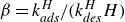 $\beta = k_{\textit{ads}}^{H}/(k_{\textit{des}}^{H} H)$
is a solubility coefficient describing the strength of adsorption relative to desorption. Larger
$\beta = k_{\textit{ads}}^{H}/(k_{\textit{des}}^{H} H)$
is a solubility coefficient describing the strength of adsorption relative to desorption. Larger
 $\beta$
values correspond to less soluble surfactants, with the surfactant behaving as insoluble for
$\beta$
values correspond to less soluble surfactants, with the surfactant behaving as insoluble for
 $\beta \gg 1$
.
$\beta \gg 1$
.
The insoluble-surfactant case is described by (2.9), (2.10) and (2.13), while the soluble-surfactant case is described by (2.9), (2.10), (2.18) and (2.19). Note that (2.9) and (2.13) are equivalent to some of the equations derived in Edmonstone, Craster & Matar (Reference Edmonstone, Craster and Matar2006) when the capillary velocity scale is chosen (i.e.
 $Ca = 1$
, where
$Ca = 1$
, where
 $Ca$
is the capillary number). Typical values for variables and parameters are presented in tables 1 and 2.
$Ca$
is the capillary number). Typical values for variables and parameters are presented in tables 1 and 2.
Order-of-magnitude estimates of important dimensional parameters.

Typical range of dimensionless parameters explored in this work using the dimensional parameter values from table 1.

2.5. Initial conditions
Motivated by prior work (Larsson & Kumar Reference Larsson and Kumar2021), we approximate the initial condition of the two-layer coating (figure 1) through two transition functions
 $T_{\textit{solute}}$
and
$T_{\textit{solute}}$
and
 $T_{\textit{surfactant}}$
, achieving the desired stratification between the component-rich and component-depleted layers
$T_{\textit{surfactant}}$
, achieving the desired stratification between the component-rich and component-depleted layers
 \begin{align} T_{\textit{solute}}(z; h_b, s) &=\!\begin{cases}1, & \text{if } w \leqslant 0 \\ \tfrac {\exp (-1/(1-w))}{\exp (-1/(1-w)) + \exp (-1/w)}, & \text{if } 0 \lt w\lt 1 \ \ \text{where } w = \tfrac {z - (h_b - 1/s)}{2/s}, \\ 0, & \text{if } 1 \leqslant w \end{cases} \end{align}
 \begin{align} T_{\textit{surfactant}}(z; h_b, s) &=\!\begin{cases} 0, &\! \text{if } w \leqslant 0 \\ 1 - \tfrac {\exp (-1/(1-w))}{\exp (-1/(1-w)) + \exp (-1/w)}, & \!\text{if } 0 \lt w\lt 1 \ \ \text{where } w = \tfrac {z - (h_b - 1/s)}{2/s}. \\ 1, &\! \text{if } 1 \leqslant w \end{cases} \end{align}
Here,
 $s$
is the slope of the transition between layers of distinct composition and
$s$
is the slope of the transition between layers of distinct composition and
 $h_b$
is the dimensionless bottom-layer thickness. We take
$h_b$
is the dimensionless bottom-layer thickness. We take
 $s= 3$
and
$s= 3$
and
 $h_b = 0.5$
to match previously chosen values for the surfactant-free case (Larsson & Kumar Reference Larsson and Kumar2021). The stratification of solute and surfactant respectively achieved by (2.22) and (2.23) can be visualised in figures 2(a) and 2(b).
$h_b = 0.5$
to match previously chosen values for the surfactant-free case (Larsson & Kumar Reference Larsson and Kumar2021). The stratification of solute and surfactant respectively achieved by (2.22) and (2.23) can be visualised in figures 2(a) and 2(b).
Transition functions for the (a) solute and (b) surfactant approximating each component’s vertical stratification. The solute concentration field at
 $t = 0$
is shown in (c), and its perturbation amplitude is amplified in (d) from
$t = 0$
is shown in (c), and its perturbation amplitude is amplified in (d) from
 $\phi _p = 0.01$
to
$\phi _p = 0.01$
to
 $\phi _p = 0.3$
so it can be seen more easily. The
$\phi _p = 0.3$
so it can be seen more easily. The
 $x$
-coordinate is rescaled from
$x$
-coordinate is rescaled from
 $[0, 2\pi /\alpha ]$
to
$[0, 2\pi /\alpha ]$
to
 $[0,1]$
.
$[0,1]$
.

The solute transition function (2.22) models a film with a solute-depleted top layer and a solute-rich bottom layer. Consistent with prior work (Larsson & Kumar Reference Larsson and Kumar2021), we refer to this as a two-layer film even though solute diffusion homogenises the two-layer structure as time progresses. In the absence of a lateral perturbation, diffusion would occur evenly across the film height. To better understand the onset and growth of non-uniformities driven by solute Marangoni stresses, we follow prior work (Larsson & Kumar Reference Larsson and Kumar2021) and introduce a lateral perturbation in the solute concentration localised at
 $z = h_b$
 \begin{equation} \phi (x, z, t = 0) = T_{\textit{solute}} \left [ 1 + \phi _p \cos (\alpha x) \exp \left (- \frac {(z - h_b)^2}{2 \nu ^2} \right ) \right ] . \end{equation}
Here,
 $\phi _p = 0.01$
is the perturbation amplitude (assumed small),
$\phi _p = 0.01$
is the perturbation amplitude (assumed small),
 $\alpha = 0.3$
is its wavenumber and
$\alpha = 0.3$
is its wavenumber and
 $\nu = 0.1$
is the standard deviation of the Gaussian localising the initial perturbation at a height
$\nu = 0.1$
is the standard deviation of the Gaussian localising the initial perturbation at a height
 $h_b$
from the substrate. This perturbation satisfies the periodic boundary conditions and corresponds to a depletion of solute at the centre of the film localised at the diffuse region between the two layers. Its localisation at
$h_b$
from the substrate. This perturbation satisfies the periodic boundary conditions and corresponds to a depletion of solute at the centre of the film localised at the diffuse region between the two layers. Its localisation at
 $z = h_b$
allows us to more easily probe the influence of solute vertical diffusion on the system’s response to the lateral disturbance, which is shown in figures 2(c) and 2(d).
$z = h_b$
allows us to more easily probe the influence of solute vertical diffusion on the system’s response to the lateral disturbance, which is shown in figures 2(c) and 2(d).
Initially, the fluid is at rest, the film is flat and the height is subject to the initial condition
 $h(x,t = 0) = 1$
. Surfactant in the insoluble case is uniformly deposited as a monolayer such that
$h(x,t = 0) = 1$
. Surfactant in the insoluble case is uniformly deposited as a monolayer such that
 $\varGamma (x,t = 0) = 1$
. To qualitatively compare our model with the experiments of Horiuchi et al. (Reference Horiuchi, Suszynski and Carvalho2015), we also investigated a configuration which involves soluble surfactant through the initial conditions
$\varGamma (x,t = 0) = 1$
. To qualitatively compare our model with the experiments of Horiuchi et al. (Reference Horiuchi, Suszynski and Carvalho2015), we also investigated a configuration which involves soluble surfactant through the initial conditions
 $\varGamma (x,t = 0) = 1$
and
$\varGamma (x,t = 0) = 1$
and
 $c(x,z,t = 0) = T_{\textit{surfactant}}$
. This corresponds to a surfactant-depleted bottom layer, a surfactant-rich top layer and equilibrium conditions at
$c(x,z,t = 0) = T_{\textit{surfactant}}$
. This corresponds to a surfactant-depleted bottom layer, a surfactant-rich top layer and equilibrium conditions at
 $t = 0$
between the surfactant-rich top layer and the liquid–air interface.
$t = 0$
between the surfactant-rich top layer and the liquid–air interface.
2.6. Numerical method
We implement a coordinate transformation to numerically handle the moving-boundary problem by mapping
 $(x,z,t) \to (\chi , \eta , \tau )$
, where
$(x,z,t) \to (\chi , \eta , \tau )$
, where
 \begin{align} \frac {\partial \chi }{\partial x} = 1, \ \ \eta = \frac {z}{h}, \ \ \frac {\partial \tau }{\partial t} = 1. \end{align}
Scaling the
 $z$
-coordinate using the height leads to a fixed-coordinate domain where the interface remains at
$z$
-coordinate using the height leads to a fixed-coordinate domain where the interface remains at
 $\eta = 1$
. Further details are given in § S.2 of supplementary material. The transformed system of equations is solved on the
$\eta = 1$
. Further details are given in § S.2 of supplementary material. The transformed system of equations is solved on the
 $[0, 2\pi /\alpha ] \times [0, 1]$
domain via a pseudospectral method (Trefethen Reference Trefethen1996). Periodicity in
$[0, 2\pi /\alpha ] \times [0, 1]$
domain via a pseudospectral method (Trefethen Reference Trefethen1996). Periodicity in
 $\chi$
warrants the use of Fourier modes for the
$\chi$
warrants the use of Fourier modes for the
 $\chi$
domain, while a finite
$\chi$
domain, while a finite
 $\eta$
domain on
$\eta$
domain on
 $[ 0, 1]$
warrants the use of Chebyshev polynomials for that domain (Boyd Reference Boyd2001). Mesh independence was achieved for the examined conditions using 50 Fourier modes or less and 150 Chebyshev polynomials or less. We used ode15s for time integration, a variable-step, variable-order implicit solver built into MATLAB. Results were validated through comparisons with prior work in the absence of surfactants (Larsson & Kumar Reference Larsson and Kumar2021).
$[ 0, 1]$
warrants the use of Chebyshev polynomials for that domain (Boyd Reference Boyd2001). Mesh independence was achieved for the examined conditions using 50 Fourier modes or less and 150 Chebyshev polynomials or less. We used ode15s for time integration, a variable-step, variable-order implicit solver built into MATLAB. Results were validated through comparisons with prior work in the absence of surfactants (Larsson & Kumar Reference Larsson and Kumar2021).
3. Simplified models
We develop two approximations to gain additional insight into the physical mechanisms underlying the evolution of height perturbations. We present these simplified models here, and in § 4 compare their predictions with numerical simulations (§ 2.6).
3.1. Vertical-averaging approximation
When
 $\epsilon ^2 \textit{Pe} \ll 1$
, vertical diffusion of the solute is rapid relative to convection. Vertical solute concentration gradients are averaged out on a much faster time scale compared with the time needed to achieve maximum deformation of the film. We employ a vertical-averaging approximation (VAA) exploiting this time-scale disparity through an asymptotic expansion in powers of
$\epsilon ^2 \textit{Pe} \ll 1$
, vertical diffusion of the solute is rapid relative to convection. Vertical solute concentration gradients are averaged out on a much faster time scale compared with the time needed to achieve maximum deformation of the film. We employ a vertical-averaging approximation (VAA) exploiting this time-scale disparity through an asymptotic expansion in powers of
 $\epsilon ^2 Pe$
 \begin{align} \phi = \phi _b (x,z,t) + \epsilon ^2 \textit{Pe} \ \phi _p (x,z,t) + \mathcal{O}\left [ \left(\epsilon ^2 \textit{Pe}\right)^2 \right ]\!. \end{align}
After substituting (3.1) into the solute convection–diffusion equation, (2.10), and employing boundary conditions (2.11) and (2.12), we recognise that
 $\phi _b$
is independent of
$\phi _b$
is independent of
 $z$
and obtain the governing equation
$z$
and obtain the governing equation
 \begin{equation} \frac {\partial \phi _b}{\partial t} + \overline {u} \frac {\partial \phi _b}{\partial x} = \frac {1}{h \ \textit{Pe}} \frac {\partial }{\partial x} \left ( h \frac {\partial \phi _b}{\partial x} \right )\!, \end{equation}
where
 \begin{equation} \overline {u} = \frac {1}{h} \int _0^h u {\rm d}z = \frac {1}{3} h^2 \frac {\partial ^3 h}{\partial x^3} - \frac {1}{2} h \left (\frac {\partial \phi _b}{\partial x} + \frac {{\textit{Ma}}_s}{\textit{Ma}} \frac {\partial \varGamma }{\partial x} \right )\!. \end{equation}
A detailed derivation is provided in § S.3 of supplementary material. Equations (2.9), (3.2) and (2.13) are solved using a one-dimensional version of the numerical method described in § 2.6 which employs a Fourier expansion of
 $\phi _b(x,t)$
,
$\phi _b(x,t)$
,
 $h(x,t)$
and
$h(x,t)$
and
 $\varGamma (x, t)$
for spatial discretisation and ode15s for time stepping. The solution is presented under the ‘VAA’ label in subsequent figures.
$\varGamma (x, t)$
for spatial discretisation and ode15s for time stepping. The solution is presented under the ‘VAA’ label in subsequent figures.
3.2. Linearised theory
When
 $\epsilon ^2 Pe \ll 1$
, vertical solute diffusion rapidly homogenises any initial vertical solute concentration gradients. By vertically averaging initial condition (2.24), we obtain
$\epsilon ^2 Pe \ll 1$
, vertical solute diffusion rapidly homogenises any initial vertical solute concentration gradients. By vertically averaging initial condition (2.24), we obtain
 \begin{align} \phi (x, t = 0) = \int _{0}^{1} \phi (x,z,t) {\rm d}z = 0.5 + \overline {\phi _p} \ \cos (\alpha x), \end{align}
where
 \begin{align} \overline {\phi _p} = \phi _p \int _0^1 T_{\textit{solute}} \exp \left [-\frac {(z - h_b)^2}{2 \nu ^2}\right ] {\rm d}z \approx 0.00125 \ll 1. \end{align}
When solute diffusion is sufficiently fast, convection can be neglected relative to lateral diffusion, reducing (2.10) to the diffusion equation
 \begin{align} \frac {\partial \phi }{\partial t} = \frac {1}{\textit{Pe}} \frac {\partial ^2 \phi }{\partial x^2}, \end{align}
where we have retained the transient term in the limit
 ${\textit{Pe}} \to 0$
by rescaling time using a diffusive time scale. Equation (3.6) is subject to the vertically averaged initial condition (3.4).
${\textit{Pe}} \to 0$
by rescaling time using a diffusive time scale. Equation (3.6) is subject to the vertically averaged initial condition (3.4).
We use separation of variables to look for a solution of the form
 $\phi (x,t) = X(x) T(t)$
. Periodic boundary conditions in the lateral direction
$\phi (x,t) = X(x) T(t)$
. Periodic boundary conditions in the lateral direction
 $x$
suggest a cosine-series expansion for the solute concentration
$x$
suggest a cosine-series expansion for the solute concentration
 \begin{equation} \phi (x,t) = \sum _{n = 0}^{\infty } a_n \exp \left (-\frac {n^2 \alpha ^2 t}{\textit{Pe}}\right ) \cos \left (n \alpha x \right )\!. \end{equation}
Initial condition (3.4) imposes
 $a_0 = 0.5$
and
$a_0 = 0.5$
and
 $a_1$
=
$a_1$
=
 $\overline {\phi _p}$
. Since higher-order terms decay exponentially fast, we substitute the leading-order solution
$\overline {\phi _p}$
. Since higher-order terms decay exponentially fast, we substitute the leading-order solution
 $\phi (x,t) = 0.5 + \overline {\phi _p} \cos (\alpha x) \exp {(-\alpha ^2 t/Pe)}$
into (2.9) and (2.13).
$\phi (x,t) = 0.5 + \overline {\phi _p} \cos (\alpha x) \exp {(-\alpha ^2 t/Pe)}$
into (2.9) and (2.13).
Since
 $\overline {\phi _p} \ll 1$
, the remaining variables are expanded in powers of
$\overline {\phi _p} \ll 1$
, the remaining variables are expanded in powers of
 $\overline {\phi _p}$
as
$\overline {\phi _p}$
as
 \begin{align} h = 1 + g(t) \overline {\phi _p} \cos (\alpha x) + \mathcal{O}[(\overline {\phi _p})^2], \end{align}
 \begin{align} \varGamma = 1 + q(t) \overline {\phi _p} \cos (\alpha x) + \mathcal{O}[(\overline {\phi _p})^2]. \end{align}
This expansion represents an initially uniform film thickness and surfactant concentration field with a small lateral perturbation.
Inserting (3.8) and (3.9) into (2.9) and (2.13) yields the
 $\mathcal{O}[\overline {\phi _p}]$
problem
$\mathcal{O}[\overline {\phi _p}]$
problem
 \begin{align} \frac {{\rm d}g(t)}{{\rm d}t} &= -\frac {1}{3} \alpha ^4 g(t) -\frac {\alpha ^2}{2} \left [ \exp \left ({-\frac {\alpha ^2 t}{\textit{Pe}}} \right ) + \frac {{\textit{Ma}}_{s}}{\textit{Ma}} q(t) \right ], \end{align}
 \begin{align} \frac {{\rm d} q(t)}{{\rm d}t} &= - q(t) \left [\alpha ^2 \frac {{\textit{Ma}}_{s}}{\textit{Ma}} + \frac {\alpha ^2 }{{\textit{Pe}}_{s}} \right ] -\frac {\alpha ^4}{2} g(t) - \alpha ^2 \exp \left (-\frac {\alpha ^2 t}{\textit{Pe}} \right )\!, \end{align}
which forms a linear system of constant-coefficient inhomogeneous ordinary differential equations. A detailed derivation along with some analytical results are provided in § S.4 of supplementary material. Solutions were obtained numerically using MATLAB’s ode15s with initial conditions
 $g(t) = q(t) = 0$
, and are presented under the ‘linearised theory’ label in subsequent figures.
$g(t) = q(t) = 0$
, and are presented under the ‘linearised theory’ label in subsequent figures.
4. Insoluble surfactant
We first consider an insoluble surfactant initially deposited uniformly at the liquid–air interface with
 $\varGamma (x,t = 0) = 1$
. Similar to prior work (Larsson & Kumar Reference Larsson and Kumar2021), we solve for the maximum height perturbation
$\varGamma (x,t = 0) = 1$
. Similar to prior work (Larsson & Kumar Reference Larsson and Kumar2021), we solve for the maximum height perturbation
 $\Delta h$
, a measure of the maximum deformation that develops, given by
$\Delta h$
, a measure of the maximum deformation that develops, given by
 \begin{equation} \Delta h =\max _{t} \{\Delta h_t: \Delta h_t = h_{\textit{max}} (t) - h_{min}(t)\}. \end{equation}
Here,
 $h_{\textit{max}}(t)$
and
$h_{\textit{max}}(t)$
and
 $h_{min}(t)$
are the maximum and minimum height over the lateral direction
$h_{min}(t)$
are the maximum and minimum height over the lateral direction
 $x$
at time
$x$
at time
 $t$
. We also solve for
$t$
. We also solve for
 $t_{\textit{max}} = \underset {t}{\text{argmax}} \ \Delta h_t$
, the time at which
$t_{\textit{max}} = \underset {t}{\text{argmax}} \ \Delta h_t$
, the time at which
 $\Delta h$
occurs.
$\Delta h$
occurs.
We stop the simulation once two conditions are met: (i) a maximum height perturbation has been achieved, and (ii) the film has nearly levelled. Condition (i) is satisfied once the height non-uniformity starts decreasing with time. This condition is described by
 $\Delta h - \Delta h_t \gt 0$
. At early times, the height perturbation grows and this criterion is not yet satisfied. Once a maximum height has been reached, the height deformation levels and
$\Delta h - \Delta h_t \gt 0$
. At early times, the height perturbation grows and this criterion is not yet satisfied. Once a maximum height has been reached, the height deformation levels and
 $\Delta h_t \lt \Delta h$
. Condition (ii) is met when
$\Delta h_t \lt \Delta h$
. Condition (ii) is met when
 $\Delta h_t \lt 10^{-5}$
for an arbitrary time duration, chosen to be ten time steps taken by the solver. In some instances, the film overshoots its levelled state before levelling off due to persistent surfactant Marangoni stresses (see § S.5 of the supplementary material). Ten time steps were sufficient to capture this delevelling phenomenon.
$\Delta h_t \lt 10^{-5}$
for an arbitrary time duration, chosen to be ten time steps taken by the solver. In some instances, the film overshoots its levelled state before levelling off due to persistent surfactant Marangoni stresses (see § S.5 of the supplementary material). Ten time steps were sufficient to capture this delevelling phenomenon.
4.1. Fast-diffusion regime
We first discuss the regime of relatively low Péclet numbers (
 ${\textit{Pe}} \lt 10^4$
), where solute diffusion is rapid enough to homogenise vertical solute concentration gradients on a much faster time scale relative to other phenomena. The initial perturbation imposed on the solute concentration profile (figure 2
c) diffuses to the solute-depleted liquid–air interface and causes a laterally inhomogeneous solute composition there. The centre of the film is depleted of solute relative to the edges and will correspond to a high-surface-tension zone (figures 3
a and 3
c). Surface-tension gradients set the liquid in motion at the initially flat interface (figure 3
b), exerting a pull toward the centre of the film. At early times, the surfactant concentration gradients at the interface are relatively weak (figure 3
d), and this solute Marangoni flow acts mostly uninhibited, easily deforming the film thickness and producing a prominent non-uniformity in the height (figure 3
b).
${\textit{Pe}} \lt 10^4$
), where solute diffusion is rapid enough to homogenise vertical solute concentration gradients on a much faster time scale relative to other phenomena. The initial perturbation imposed on the solute concentration profile (figure 2
c) diffuses to the solute-depleted liquid–air interface and causes a laterally inhomogeneous solute composition there. The centre of the film is depleted of solute relative to the edges and will correspond to a high-surface-tension zone (figures 3
a and 3
c). Surface-tension gradients set the liquid in motion at the initially flat interface (figure 3
b), exerting a pull toward the centre of the film. At early times, the surfactant concentration gradients at the interface are relatively weak (figure 3
d), and this solute Marangoni flow acts mostly uninhibited, easily deforming the film thickness and producing a prominent non-uniformity in the height (figure 3
b).
Profiles of (a) surface tension
 $\sigma$
, (b) height
$\sigma$
, (b) height
 $h$
, (c) interface solute concentration
$h$
, (c) interface solute concentration
 $\phi |_{z = h}$
and (d) interface surfactant concentration
$\phi |_{z = h}$
and (d) interface surfactant concentration
 $\varGamma$
for the insoluble case at various times. Here,
$\varGamma$
for the insoluble case at various times. Here,
 $Ma = 0.01$
,
$Ma = 0.01$
,
 ${\textit{Pe}} = 5 \times 10^3$
,
${\textit{Pe}} = 5 \times 10^3$
,
 ${\textit{Pe}}_s = 10^3$
and
${\textit{Pe}}_s = 10^3$
and
 ${\textit{Ma}}_{s} = 0.001$
. The surface tension and the interface solute concentration at
${\textit{Ma}}_{s} = 0.001$
. The surface tension and the interface solute concentration at
 $t = 0$
are horizontal lines at
$t = 0$
are horizontal lines at
 $0.999$
and
$0.999$
and
 $0$
, respectively, and were left out of (a) and (c) for clarity.
$0$
, respectively, and were left out of (a) and (c) for clarity.

Solute Marangoni flow redistributes surfactant so that it is more concentrated at the centre of the film relative to the edges (figure 3 d). Since surfactant lowers the surface tension, surface-tension gradients arising from solute Marangoni effects are weakened by this surfactant redistribution. In addition, surfactant concentration gradients drive Marangoni stresses that oppose solute Marangoni stresses. Given that solute-driven convection is responsible for the deformation of the initially flat interface, surfactants resist the growth of film-height perturbations.
The competition between solute and surfactant Marangoni flows can be understood through the influence of each species on the change in height as described by (2.9). The two Marangoni contributions in (2.9) are of opposite signs given the opposite direction of their interface concentration gradients. We compare the relative magnitude of each Marangoni flow through the respective solute and surfactant contribution terms,
 $1/2 \ \partial _x [h^2 \ \partial _x(\phi |_{z = h})]$
and
$1/2 \ \partial _x [h^2 \ \partial _x(\phi |_{z = h})]$
and
 $1/2({\textit{Ma}}_{s}/Ma)\partial _x [h^2 \partial _x \varGamma ]$
, where
$1/2({\textit{Ma}}_{s}/Ma)\partial _x [h^2 \partial _x \varGamma ]$
, where
 $\partial _x = \partial /\partial x$
. We compute the maximum gradient in absolute value over all
$\partial _x = \partial /\partial x$
. We compute the maximum gradient in absolute value over all
 $x$
-coordinate nodes for each time
$x$
-coordinate nodes for each time
 $t$
using a fourth-order centred finite-difference scheme and plot the result versus time for different
$t$
using a fourth-order centred finite-difference scheme and plot the result versus time for different
 ${\textit{Ma}}_s$
in figure 4. As
${\textit{Ma}}_s$
in figure 4. As
 ${\textit{Ma}}_s$
increases, the maximum solute contribution decreases at any given time while the surfactant contribution increases.
${\textit{Ma}}_s$
increases, the maximum solute contribution decreases at any given time while the surfactant contribution increases.
Figure 5(a) shows the resulting monotonic decrease in
 $\Delta h$
, the maximum amplitude of the interface deformation, with increasing
$\Delta h$
, the maximum amplitude of the interface deformation, with increasing
 ${\textit{Ma}}_{s}$
. This behaviour is consistent with the suppression mechanisms just described. From figure 5(c), we observe that surfactant decreases
${\textit{Ma}}_{s}$
. This behaviour is consistent with the suppression mechanisms just described. From figure 5(c), we observe that surfactant decreases
 $t_{\textit{max}}$
, the time at which the maximum perturbation is reached. At low
$t_{\textit{max}}$
, the time at which the maximum perturbation is reached. At low
 ${\textit{Ma}}_s$
, increasing
${\textit{Ma}}_s$
, increasing
 ${\textit{Pe}}$
leads to larger height deformations
${\textit{Pe}}$
leads to larger height deformations
 $\Delta h$
and higher
$\Delta h$
and higher
 $t_{\textit{max}}$
. This is because the lateral solute diffusive time scale increases with
$t_{\textit{max}}$
. This is because the lateral solute diffusive time scale increases with
 ${\textit{Pe}}$
and sustains solute concentration gradients at the interface for a longer time. This effect exacerbates solute Marangoni stresses and delays the erasure of solute concentration gradients by lateral diffusion, producing larger
${\textit{Pe}}$
and sustains solute concentration gradients at the interface for a longer time. This effect exacerbates solute Marangoni stresses and delays the erasure of solute concentration gradients by lateral diffusion, producing larger
 $\Delta h$
and leading to higher
$\Delta h$
and leading to higher
 $t_{\textit{max}}$
. The film’s behaviour at high
$t_{\textit{max}}$
. The film’s behaviour at high
 ${\textit{Ma}}_s$
, which appears independent of
${\textit{Ma}}_s$
, which appears independent of
 ${\textit{Pe}}$
, is discussed through a scaling argument in § 4.1.2.
${\textit{Pe}}$
, is discussed through a scaling argument in § 4.1.2.
Time evolution of (a) solute and (b) surfactant contributions to the change in height (second and third terms in (2.9)) for various
 ${\textit{Ma}}_{s}$
with
${\textit{Ma}}_{s}$
with
 $Ma = 0.01$
,
$Ma = 0.01$
,
 ${\textit{Pe}} = 5 \times 10^3$
and
${\textit{Pe}} = 5 \times 10^3$
and
 ${\textit{Pe}}_s = 10^3$
.
${\textit{Pe}}_s = 10^3$
.

Variation of (a)
 $\Delta h$
and (c)
$\Delta h$
and (c)
 $t_{\textit{max}}$
with
$t_{\textit{max}}$
with
 ${\textit{Ma}}_{s}$
for various Péclet numbers in the regime of fast solute diffusion. Comparison of (b)
${\textit{Ma}}_{s}$
for various Péclet numbers in the regime of fast solute diffusion. Comparison of (b)
 $\Delta h$
and (d)
$\Delta h$
and (d)
 $t_{\textit{max}}$
between the linearised theory, VAA and 2-D model for
$t_{\textit{max}}$
between the linearised theory, VAA and 2-D model for
 ${\textit{Pe}} = 100$
. The other parameters are fixed at
${\textit{Pe}} = 100$
. The other parameters are fixed at
 $Ma = 0.01$
and
$Ma = 0.01$
and
 ${\textit{Pe}}_s = 10^4$
. Note that the range
${\textit{Pe}}_s = 10^4$
. Note that the range
 $0.1 \lt {\textit{Ma}}_{s} \lt 0.9$
was investigated to gain insight into asymptotic behaviour at very high surfactant mass fractions.
$0.1 \lt {\textit{Ma}}_{s} \lt 0.9$
was investigated to gain insight into asymptotic behaviour at very high surfactant mass fractions.

4.1.1. Accuracy of simplified models
Figures 5(b) and 5(d) compare predictions of the two simplified models developed in § 3 with the two-dimensional (2-D) model. The simplified models agree with the 2-D model for
 ${\textit{Pe}} = 100$
(shown), and to within
${\textit{Pe}} = 100$
(shown), and to within
 $10\,\%$
for larger values of
$10\,\%$
for larger values of
 ${\textit{Pe}} \lt 10^4$
(not shown). At first glance, this result is surprising given the assumption
${\textit{Pe}} \lt 10^4$
(not shown). At first glance, this result is surprising given the assumption
 $\epsilon ^2 Pe \ll 1$
in the derivation of the VAA, and the additional assumption of dominant lateral solute diffusion over convective effects for the linearised theory. The latter assumption requires
$\epsilon ^2 Pe \ll 1$
in the derivation of the VAA, and the additional assumption of dominant lateral solute diffusion over convective effects for the linearised theory. The latter assumption requires
 ${\textit{Pe}} \ll 1$
. The observed accuracy up to
${\textit{Pe}} \ll 1$
. The observed accuracy up to
 ${\textit{Pe}} = 10^4$
suggests that the height non-uniformity can be accurately predicted while neglecting both the vertical stratification of the solute and convective terms. We note that the maximum deformation values are relatively small due to the relatively small amplitude of the initial concentration perturbation (
${\textit{Pe}} = 10^4$
suggests that the height non-uniformity can be accurately predicted while neglecting both the vertical stratification of the solute and convective terms. We note that the maximum deformation values are relatively small due to the relatively small amplitude of the initial concentration perturbation (
 $\phi _p= 0.01$
; see § 2.5). Larger initial perturbations lead to larger height deformations, but also larger concentration gradients in both the vertical and horizontal directions. These gradients are computationally challenging to accurately resolve, so they are not investigated here.
$\phi _p= 0.01$
; see § 2.5). Larger initial perturbations lead to larger height deformations, but also larger concentration gradients in both the vertical and horizontal directions. These gradients are computationally challenging to accurately resolve, so they are not investigated here.
In the fast-diffusion regime, vertical solute concentration gradients are erased rapidly enough so that the two-layer structure behaves as one layer. Vertical solute concentration gradients are homogenised on a time scale of
 $\epsilon ^2 Pe \lt 100$
for
$\epsilon ^2 Pe \lt 100$
for
 $\epsilon = 0.1$
and
$\epsilon = 0.1$
and
 ${\textit{Pe}} \lt 10^4$
, which is much faster than
${\textit{Pe}} \lt 10^4$
, which is much faster than
 $t_{\textit{max}} \geqslant 600$
at low
$t_{\textit{max}} \geqslant 600$
at low
 ${\textit{Ma}}_s$
(figure 5
d). Since
${\textit{Ma}}_s$
(figure 5
d). Since
 $\epsilon ^2 Pe \ll t_{\textit{max}}$
, the simplified models exploit the disparity between the vertical-diffusion time scale and the time needed to achieve the maximum height deformation by treating the stratified system as a single layer. The VAA employs a 1-D expansion of variables in Fourier modes starting from a vertically uniform initial solute concentration profile, but can achieve comparable accuracy to the 2-D model in this regime of fast solute diffusion. This significantly reduces the computational expense of resolving a vertical solute stratification, which requires a high-order Chebyshev polynomial expansion to accurately describe the solute concentration profile in the vertical direction.
$\epsilon ^2 Pe \ll t_{\textit{max}}$
, the simplified models exploit the disparity between the vertical-diffusion time scale and the time needed to achieve the maximum height deformation by treating the stratified system as a single layer. The VAA employs a 1-D expansion of variables in Fourier modes starting from a vertically uniform initial solute concentration profile, but can achieve comparable accuracy to the 2-D model in this regime of fast solute diffusion. This significantly reduces the computational expense of resolving a vertical solute stratification, which requires a high-order Chebyshev polynomial expansion to accurately describe the solute concentration profile in the vertical direction.
The
 ${\textit{Pe}}$
cutoff value of
${\textit{Pe}}$
cutoff value of
 $10^4$
matches the previously reported value for the surfactant-free case (Larsson & Kumar Reference Larsson and Kumar2021), which suggests surfactant presence does not shift this threshold. This makes sense given that the accuracy threshold is largely determined by vertical diffusion of solute from the solute-rich bottom layer to the solute-depleted interface. This diffusion mechanism is controlled by
$10^4$
matches the previously reported value for the surfactant-free case (Larsson & Kumar Reference Larsson and Kumar2021), which suggests surfactant presence does not shift this threshold. This makes sense given that the accuracy threshold is largely determined by vertical diffusion of solute from the solute-rich bottom layer to the solute-depleted interface. This diffusion mechanism is controlled by
 ${\textit{Pe}}$
(Larsson & Kumar Reference Larsson and Kumar2021) and is not significantly affected by the surfactant, which is confined to the interface in the insoluble case. As a result, the accuracy threshold defined for the simplified models is insensitive to surfactant redistribution and
${\textit{Pe}}$
(Larsson & Kumar Reference Larsson and Kumar2021) and is not significantly affected by the surfactant, which is confined to the interface in the insoluble case. As a result, the accuracy threshold defined for the simplified models is insensitive to surfactant redistribution and
 ${\textit{Ma}}_s$
, and is instead primarily controlled by
${\textit{Ma}}_s$
, and is instead primarily controlled by
 ${\textit{Pe}}$
.
${\textit{Pe}}$
.
4.1.2. Asymptotic behaviour at high
 ${\textit{Ma}}_s$

From figures 5(a) and 5(b), we note
 $\Delta h \sim {\textit{Ma}}_{s}^{-1}$
when
$\Delta h \sim {\textit{Ma}}_{s}^{-1}$
when
 ${\textit{Ma}}_{s} \gt 0.01$
. This is consistent with the asymptotic behaviour of the function
${\textit{Ma}}_{s} \gt 0.01$
. This is consistent with the asymptotic behaviour of the function
 $g(t)$
in (3.10), which describes the time dependence of the height perturbation in the linearised theory. It is straightforward to show that in the limit
$g(t)$
in (3.10), which describes the time dependence of the height perturbation in the linearised theory. It is straightforward to show that in the limit
 $b = {\textit{Ma}}_s/Ma \gg 1$
(see § S.4 of supplementary material for details)
$b = {\textit{Ma}}_s/Ma \gg 1$
(see § S.4 of supplementary material for details)
 \begin{align} \Delta h \sim b ^{-1} . \end{align}
The regime where the linear slope is observed in figure 5(a) corresponds to
 $b \geqslant 1$
. Scaling relation (4.2) reflects the fact that stronger surfactant Marangoni stresses at increasing
$b \geqslant 1$
. Scaling relation (4.2) reflects the fact that stronger surfactant Marangoni stresses at increasing
 ${\textit{Ma}}_{s}$
(larger
${\textit{Ma}}_{s}$
(larger
 $b$
) lead to smaller height non-uniformities (smaller
$b$
) lead to smaller height non-uniformities (smaller
 $g(t_{\textit{max}})$
and thus smaller
$g(t_{\textit{max}})$
and thus smaller
 $\Delta h$
) that are more rapidly attained (smaller
$\Delta h$
) that are more rapidly attained (smaller
 $t_{\textit{max}}$
, figures 5
c and 5
d).
$t_{\textit{max}}$
, figures 5
c and 5
d).
Figure 5(a) also shows nearly overlapping
 $\Delta h$
plots at high
$\Delta h$
plots at high
 ${\textit{Ma}}_s$
as
${\textit{Ma}}_s$
as
 ${\textit{Pe}}$
varies over two orders of magnitude. Scaling relation (S.73) in the supplementary material suggests that
${\textit{Pe}}$
varies over two orders of magnitude. Scaling relation (S.73) in the supplementary material suggests that
 $\Delta h$
is relatively insensitive to
$\Delta h$
is relatively insensitive to
 ${\textit{Pe}}$
in the fast-diffusion regime when
${\textit{Pe}}$
in the fast-diffusion regime when
 $b \gg 1$
, since
$b \gg 1$
, since
 \begin{align} \Delta h \sim \exp \left (-t_{\textit{max}} \frac {\alpha ^2}{\textit{Pe}}\right )\!. \end{align}
The argument of the exponential in (4.3) is responsible for the influence of
 ${\textit{Pe}}$
on
${\textit{Pe}}$
on
 $\Delta h$
. For typical values
$\Delta h$
. For typical values
 $\alpha = 0.3$
,
$\alpha = 0.3$
,
 $t_{\textit{max}} \leqslant 1000$
and
$t_{\textit{max}} \leqslant 1000$
and
 $100 \leqslant Pe \leqslant 10^4$
, we obtain
$100 \leqslant Pe \leqslant 10^4$
, we obtain
 $ t_{\textit{max}} \alpha ^2/Pe \leqslant 0.9$
. In contrast, the effect of surfactant Marangoni stresses on
$ t_{\textit{max}} \alpha ^2/Pe \leqslant 0.9$
. In contrast, the effect of surfactant Marangoni stresses on
 $\Delta h$
is given by (S.74) of supplementary material as
$\Delta h$
is given by (S.74) of supplementary material as
 \begin{align} \Delta h \sim \exp \left (-b \alpha ^2 t_{\textit{max}}\right )\!. \end{align}
From figure 5(a), we note that surfactants exert a significant influence on
 $\Delta h$
when
$\Delta h$
when
 ${\textit{Ma}}_s \geqslant 0.001$
(
${\textit{Ma}}_s \geqslant 0.001$
(
 $b \geqslant 0.1$
). In this regime, the exponential argument in (4.4) exceeds
$b \geqslant 0.1$
). In this regime, the exponential argument in (4.4) exceeds
 $9$
. This value is an order of magnitude larger than the exponential argument responsible for
$9$
. This value is an order of magnitude larger than the exponential argument responsible for
 ${\textit{Pe}}$
effects (
${\textit{Pe}}$
effects (
 $9/0.9 = 10$
). We thus expect that variations in
$9/0.9 = 10$
). We thus expect that variations in
 ${\textit{Pe}}$
will have negligible influence on the maximum height non-uniformity in this regime compared with
${\textit{Pe}}$
will have negligible influence on the maximum height non-uniformity in this regime compared with
 ${\textit{Ma}}_s$
. We also note that (4.3) quickly approaches
${\textit{Ma}}_s$
. We also note that (4.3) quickly approaches
 $0$
as
$0$
as
 ${\textit{Pe}} \to 0$
, revealing that
${\textit{Pe}} \to 0$
, revealing that
 $\Delta h$
is insensitive to
$\Delta h$
is insensitive to
 ${\textit{Pe}}$
relative to other parameters when solute diffusion is sufficiently fast. This reasoning agrees with prior work on films devoid of surfactant (Larsson & Kumar Reference Larsson and Kumar2021) and generalises the dependence of
${\textit{Pe}}$
relative to other parameters when solute diffusion is sufficiently fast. This reasoning agrees with prior work on films devoid of surfactant (Larsson & Kumar Reference Larsson and Kumar2021) and generalises the dependence of
 $\Delta h$
on
$\Delta h$
on
 ${\textit{Pe}}$
to the surfactant-laden case.
${\textit{Pe}}$
to the surfactant-laden case.
Physically, scaling relation (4.3) can be interpreted as follows. In the low-
 ${\textit{Pe}}$
regime, vertical diffusion of solute is rapid. The initial lateral perturbation imposed on the solute and localised at
${\textit{Pe}}$
regime, vertical diffusion of solute is rapid. The initial lateral perturbation imposed on the solute and localised at
 $h_b = 0.5$
will diffuse to the interface on a much faster time scale compared with the time needed for Marangoni flows to develop laterally and drive a height non-uniformity. As a result, one-layer predictions are accurate despite treating vertical diffusion as instantaneous in the asymptotic limit of
$h_b = 0.5$
will diffuse to the interface on a much faster time scale compared with the time needed for Marangoni flows to develop laterally and drive a height non-uniformity. As a result, one-layer predictions are accurate despite treating vertical diffusion as instantaneous in the asymptotic limit of
 ${\textit{Pe}} \to 0$
and employing a vertically uniform initial condition that ignores the initial solute stratification altogether.
${\textit{Pe}} \to 0$
and employing a vertically uniform initial condition that ignores the initial solute stratification altogether.
4.2. Slow-diffusion regime
4.2.1. Behaviour of
$\Delta h$
and
$t_{\textit{max}}$


Figure 6(a–d) shows the behaviour of
 $\Delta h$
and
$\Delta h$
and
 $t_{\textit{max}}$
with respect to
$t_{\textit{max}}$
with respect to
 ${\textit{Ma}}_s$
when
${\textit{Ma}}_s$
when
 ${\textit{Pe}} \gt 10^4$
. A monotonic decrease of
${\textit{Pe}} \gt 10^4$
. A monotonic decrease of
 $\Delta h$
with increasing
$\Delta h$
with increasing
 ${\textit{Ma}}_{s}$
is observed (figures 6
a and 6
b), consistent with trends reported in the low-
${\textit{Ma}}_{s}$
is observed (figures 6
a and 6
b), consistent with trends reported in the low-
 ${\textit{Pe}}$
regime (§ 4.1). In contrast,
${\textit{Pe}}$
regime (§ 4.1). In contrast,
 $t_{\textit{max}}$
tends to plateau at
$t_{\textit{max}}$
tends to plateau at
 ${\textit{Ma}}_s \geqslant 0.01$
in the high-
${\textit{Ma}}_s \geqslant 0.01$
in the high-
 ${\textit{Pe}}$
regime (figures 6
c and 6
d).
${\textit{Pe}}$
regime (figures 6
c and 6
d).
Variation of (a)
 $\Delta h$
and (c)
$\Delta h$
and (c)
 $t_{\textit{max}}$
with
$t_{\textit{max}}$
with
 ${\textit{Ma}}_{s}$
for various Péclet numbers in the regime of slow solute diffusion. Comparison of (b)
${\textit{Ma}}_{s}$
for various Péclet numbers in the regime of slow solute diffusion. Comparison of (b)
 $\Delta h$
and (d)
$\Delta h$
and (d)
 $t_{\textit{max}}$
between the linearised theory, VAA and 2-D model for
$t_{\textit{max}}$
between the linearised theory, VAA and 2-D model for
 ${\textit{Pe}} = 8 \times 10^4$
. The other parameters are fixed at
${\textit{Pe}} = 8 \times 10^4$
. The other parameters are fixed at
 ${\textit{Pe}}_s = 10^4$
and
${\textit{Pe}}_s = 10^4$
and
 $Ma = 0.01$
.
$Ma = 0.01$
.

The behaviour at low
 ${\textit{Ma}}_s$
in the high-
${\textit{Ma}}_s$
in the high-
 ${\textit{Pe}}$
regime can be understood from results obtained in previous work where surfactants were absent (corresponding to
${\textit{Pe}}$
regime can be understood from results obtained in previous work where surfactants were absent (corresponding to
 ${\textit{Ma}}_s=0$
) (Larsson & Kumar Reference Larsson and Kumar2021). In this regime, solute diffusion is slow compared with the low-
${\textit{Ma}}_s=0$
) (Larsson & Kumar Reference Larsson and Kumar2021). In this regime, solute diffusion is slow compared with the low-
 ${\textit{Pe}}$
regime, so vertical concentration gradients remain important for longer time and contribute to the developing height non-uniformity. As a consequence, the values of
${\textit{Pe}}$
regime, so vertical concentration gradients remain important for longer time and contribute to the developing height non-uniformity. As a consequence, the values of
 $\Delta h$
and
$\Delta h$
and
 $t_{\textit{max}}$
are more sensitive to the value of
$t_{\textit{max}}$
are more sensitive to the value of
 ${\textit{Pe}}$
at low
${\textit{Pe}}$
at low
 ${\textit{Ma}}_s$
(figures 6
a and 6
c) compared with the low-
${\textit{Ma}}_s$
(figures 6
a and 6
c) compared with the low-
 ${\textit{Pe}}$
regime (figures 5
a and 5
c). Moreover, the values of
${\textit{Pe}}$
regime (figures 5
a and 5
c). Moreover, the values of
 $\Delta h$
at low
$\Delta h$
at low
 ${\textit{Ma}}_s$
are generally larger in the high-
${\textit{Ma}}_s$
are generally larger in the high-
 ${\textit{Pe}}$
regime because weaker solute diffusion exacerbates lateral gradients in the solute concentration at the interface. This effect makes it easier for solute-induced Marangoni stresses to deform the interface as previously reported (Larsson & Kumar Reference Larsson and Kumar2021). Since the interface is initially solute depleted, weaker diffusion of solute at increasing
${\textit{Pe}}$
regime because weaker solute diffusion exacerbates lateral gradients in the solute concentration at the interface. This effect makes it easier for solute-induced Marangoni stresses to deform the interface as previously reported (Larsson & Kumar Reference Larsson and Kumar2021). Since the interface is initially solute depleted, weaker diffusion of solute at increasing
 ${\textit{Pe}}$
delays the onset of solute Marangoni stresses, which is reflected in the larger values of
${\textit{Pe}}$
delays the onset of solute Marangoni stresses, which is reflected in the larger values of
 $t_{\textit{max}}$
as
$t_{\textit{max}}$
as
 ${\textit{Pe}}$
increases (figures 6
b and 6
d). Additionally, since the interface deforms more as
${\textit{Pe}}$
increases (figures 6
b and 6
d). Additionally, since the interface deforms more as
 ${\textit{Pe}}$
increases, it takes longer to reach its maximum deformation, contributing to larger
${\textit{Pe}}$
increases, it takes longer to reach its maximum deformation, contributing to larger
 $t_{\textit{max}}$
at higher
$t_{\textit{max}}$
at higher
 ${\textit{Pe}}$
. Note that the
${\textit{Pe}}$
. Note that the
 $t_{\textit{max}}$
values at low
$t_{\textit{max}}$
values at low
 ${\textit{Ma}}_s$
and high
${\textit{Ma}}_s$
and high
 ${\textit{Pe}}$
can actually be smaller than those in the low-
${\textit{Pe}}$
can actually be smaller than those in the low-
 ${\textit{Pe}}$
regime due to the convective steepening of lateral solute concentration gradients driven by solute Marangoni stresses (Larsson & Kumar Reference Larsson and Kumar2021).
${\textit{Pe}}$
regime due to the convective steepening of lateral solute concentration gradients driven by solute Marangoni stresses (Larsson & Kumar Reference Larsson and Kumar2021).
As might be expected, predictions of the simplified models, which assume a vertically uniform solute concentration, deviate from the 2-D model predictions at low
 ${\textit{Ma}}_s$
in the high-
${\textit{Ma}}_s$
in the high-
 ${\textit{Pe}}$
regime (figures 6
b and 6
d), in contrast to the excellent agreement observed in the low-
${\textit{Pe}}$
regime (figures 6
b and 6
d), in contrast to the excellent agreement observed in the low-
 ${\textit{Pe}}$
regime (figures 5
b and 5
d). However, the values of
${\textit{Pe}}$
regime (figures 5
b and 5
d). However, the values of
 $\Delta h$
become relatively independent of
$\Delta h$
become relatively independent of
 ${\textit{Pe}}$
at high
${\textit{Pe}}$
at high
 ${\textit{Ma}}_s$
(figure 6
a) and agree closely with predictions of simplified models in this regime (figure 6
c). This suggests that sufficiently strong surfactant Marangoni flows can help erase vertical solute concentration gradients and produce a quasi-one-layer structure, as discussed below.
${\textit{Ma}}_s$
(figure 6
a) and agree closely with predictions of simplified models in this regime (figure 6
c). This suggests that sufficiently strong surfactant Marangoni flows can help erase vertical solute concentration gradients and produce a quasi-one-layer structure, as discussed below.
4.2.2. Marangoni-induced recirculation
To better understand the high-
 ${\textit{Pe}}$
regime, we plot the velocity field and solute concentration contours in figures 7 and 8 for various parameter values. For reference, we first consider the low-
${\textit{Pe}}$
regime, we plot the velocity field and solute concentration contours in figures 7 and 8 for various parameter values. For reference, we first consider the low-
 ${\textit{Pe}}$
regime in figure 7. When
${\textit{Pe}}$
regime in figure 7. When
 $t \approx 0.5 \, t_{\textit{max}}$
(figure 7
a), rapid vertical diffusion has already eliminated steep vertical concentration gradients. The resulting horizontal concentration gradients drive Marangoni flow toward the film centre. When
$t \approx 0.5 \, t_{\textit{max}}$
(figure 7
a), rapid vertical diffusion has already eliminated steep vertical concentration gradients. The resulting horizontal concentration gradients drive Marangoni flow toward the film centre. When
 $ t \approx 1.5 \, t_{\textit{max}}$
(figure 7
b), the film has already achieved a maximum height deformation at
$ t \approx 1.5 \, t_{\textit{max}}$
(figure 7
b), the film has already achieved a maximum height deformation at
 $t_{\textit{max}}$
and is in the process of relaxing back to a flat state with flow directed away from the height peak at the film centre. Surfactant has already accumulated at the centre of the film by this time, so surfactant Marangoni flows and capillary levelling act to recover a flat film. The general behaviour shown here is representative of other values of
$t_{\textit{max}}$
and is in the process of relaxing back to a flat state with flow directed away from the height peak at the film centre. Surfactant has already accumulated at the centre of the film by this time, so surfactant Marangoni flows and capillary levelling act to recover a flat film. The general behaviour shown here is representative of other values of
 ${\textit{Ma}}_s$
, with larger values of
${\textit{Ma}}_s$
, with larger values of
 ${\textit{Ma}}_s$
leading to smaller values of
${\textit{Ma}}_s$
leading to smaller values of
 $\Delta h$
and
$\Delta h$
and
 $t_{\textit{max}}$
.
$t_{\textit{max}}$
.
Velocity field plotted over solute concentration contours at (a)
 $t \approx 24 \approx 0.5 \, t_{\textit{max}}$
and (b)
$t \approx 24 \approx 0.5 \, t_{\textit{max}}$
and (b)
 $t \approx 72 \approx 1.5 \, t_{\textit{max}}$
for
$t \approx 72 \approx 1.5 \, t_{\textit{max}}$
for
 ${\textit{Pe}} = 10^3$
. Other parameters are
${\textit{Pe}} = 10^3$
. Other parameters are
 $Ma = 0.01$
,
$Ma = 0.01$
,
 ${\textit{Ma}}_s = 0.01$
and
${\textit{Ma}}_s = 0.01$
and
 ${\textit{Pe}}_s = 10^4$
. At
${\textit{Pe}}_s = 10^4$
. At
 $t \approx 0.8 \, t_{\textit{max}}$
, the velocity field looks very similar to (a) and is not shown for brevity.
$t \approx 0.8 \, t_{\textit{max}}$
, the velocity field looks very similar to (a) and is not shown for brevity.

Velocity field plotted over solute concentration contours at
 ${\textit{Pe}} = 10^5$
,
${\textit{Pe}} = 10^5$
,
 $Ma = 0.01$
and
$Ma = 0.01$
and
 ${\textit{Pe}}_s = 10^4$
. Panels show (a)
${\textit{Pe}}_s = 10^4$
. Panels show (a)
 ${\textit{Ma}}_s = 0$
at
${\textit{Ma}}_s = 0$
at
 $t \approx 374 \approx 0.5 \,t_{\textit{max}}$
; (b)
$t \approx 374 \approx 0.5 \,t_{\textit{max}}$
; (b)
 ${\textit{Ma}}_s = 0$
at
${\textit{Ma}}_s = 0$
at
 $t \approx 599 \approx 0.8 \,t_{\textit{max}}$
; (c)
$t \approx 599 \approx 0.8 \,t_{\textit{max}}$
; (c)
 ${\textit{Ma}}_s = 0.01$
at
${\textit{Ma}}_s = 0.01$
at
 $t \approx 101 \approx 0.5 \,t_{\textit{max}}$
; (d)
$t \approx 101 \approx 0.5 \,t_{\textit{max}}$
; (d)
 ${\textit{Ma}}_s = 0.01$
at
${\textit{Ma}}_s = 0.01$
at
 $t \approx 160 \approx 0.8 \,t_{\textit{max}}$
.
$t \approx 160 \approx 0.8 \,t_{\textit{max}}$
.

Velocity magnitude contours at
 ${\textit{Pe}} = 10^5$
and
${\textit{Pe}} = 10^5$
and
 $Ma = 0.01$
when (a)
$Ma = 0.01$
when (a)
 ${\textit{Ma}}_s = 0$
and
${\textit{Ma}}_s = 0$
and
 $t \approx 0.8 \, t_{\textit{max}}$
(
$t \approx 0.8 \, t_{\textit{max}}$
(
 $t_{\textit{max}} \approx 751$
), (b)
$t_{\textit{max}} \approx 751$
), (b)
 ${\textit{Ma}}_s = 0$
and
${\textit{Ma}}_s = 0$
and
 $t \approx 0.9 \, t_{\textit{max}}$
, (c)
$t \approx 0.9 \, t_{\textit{max}}$
, (c)
 ${\textit{Ma}}_s = 0.01$
and
${\textit{Ma}}_s = 0.01$
and
 $t \approx 0.8 \, t_{\textit{max}}$
(
$t \approx 0.8 \, t_{\textit{max}}$
(
 $t_{\textit{max}} \approx 200$
), (d)
$t_{\textit{max}} \approx 200$
), (d)
 ${\textit{Ma}}_s = 0.01$
and
${\textit{Ma}}_s = 0.01$
and
 $t \approx 0.9 \, t_{\textit{max}}$
.
$t \approx 0.9 \, t_{\textit{max}}$
.

We now consider the high-
 ${\textit{Pe}}$
regime in figure 8. In figures 8(a) and 8(b), we observe sharp vertical concentration gradients when
${\textit{Pe}}$
regime in figure 8. In figures 8(a) and 8(b), we observe sharp vertical concentration gradients when
 ${\textit{Ma}}_s = 0$
. At the times shown, flow is directed toward the film centre, similar to the low-
${\textit{Ma}}_s = 0$
. At the times shown, flow is directed toward the film centre, similar to the low-
 ${\textit{Pe}}$
regime (figure 7
a) but with a vertically stratified solute concentration. The picture is dramatically different for sufficiently large
${\textit{Pe}}$
regime (figure 7
a) but with a vertically stratified solute concentration. The picture is dramatically different for sufficiently large
 ${\textit{Ma}}_s$
, as seen in figures 8(c) and 8(d). Although there are significant vertical concentration gradients when
${\textit{Ma}}_s$
, as seen in figures 8(c) and 8(d). Although there are significant vertical concentration gradients when
 $t \approx 0.5 \, t_{\textit{max}}$
, those vertical concentration gradients are rapidly smoothed out by the time
$t \approx 0.5 \, t_{\textit{max}}$
, those vertical concentration gradients are rapidly smoothed out by the time
 $t \approx 0.8 \,t_{\textit{max}}$
. Additionally, while the flow is directed toward the film centre when
$t \approx 0.8 \,t_{\textit{max}}$
. Additionally, while the flow is directed toward the film centre when
 $t \approx 0.5 \, t_{\textit{max}}$
, a recirculation region is seen when
$t \approx 0.5 \, t_{\textit{max}}$
, a recirculation region is seen when
 $t \approx 0.8 \, t_{\textit{max}}$
. This recirculation mixes the vertically stratified solute and erases its vertical concentration gradients. As a consequence, predictions of
$t \approx 0.8 \, t_{\textit{max}}$
. This recirculation mixes the vertically stratified solute and erases its vertical concentration gradients. As a consequence, predictions of
 $\Delta h$
at sufficiently high
$\Delta h$
at sufficiently high
 ${\textit{Ma}}_s$
approach those obtained from simplified one-layer models (figure 6
b).
${\textit{Ma}}_s$
approach those obtained from simplified one-layer models (figure 6
b).
In figures 9(a) and 9(c), we show velocity magnitude contours corresponding to figures 8(b) and 8(d). When
 ${\textit{Ma}}_s = 0$
, the largest velocities are located at the liquid–air interface for
${\textit{Ma}}_s = 0$
, the largest velocities are located at the liquid–air interface for
 $t \lt t_{\textit{max}}$
(figures 9
a and 9
b). As
$t \lt t_{\textit{max}}$
(figures 9
a and 9
b). As
 $t$
approaches
$t$
approaches
 $t_{\textit{max}}$
, the significant height deformation produced at high
$t_{\textit{max}}$
, the significant height deformation produced at high
 ${\textit{Pe}}$
results in large capillary stresses that resist further height deformation. Although this is not immediately apparent from figure 9(b), recirculation regions are present at
${\textit{Pe}}$
results in large capillary stresses that resist further height deformation. Although this is not immediately apparent from figure 9(b), recirculation regions are present at
 $t \approx 0.9 \, t_{\textit{max}}$
, similar to what has been previously reported for surfactant-free systems at high
$t \approx 0.9 \, t_{\textit{max}}$
, similar to what has been previously reported for surfactant-free systems at high
 ${\textit{Pe}}$
for times approaching
${\textit{Pe}}$
for times approaching
 $t_{\textit{max}}$
(Larsson & Kumar Reference Larsson and Kumar2021). However, when
$t_{\textit{max}}$
(Larsson & Kumar Reference Larsson and Kumar2021). However, when
 ${\textit{Ma}}_s = 0.01$
, the largest velocities are near the film centre, and flow at the liquid-air interface is nearly stagnant (figures 9
c and 9
d). This is due to surfactant-induced Marangoni stresses effectively resisting the solute-induced Marangoni stresses when the value of
${\textit{Ma}}_s = 0.01$
, the largest velocities are near the film centre, and flow at the liquid-air interface is nearly stagnant (figures 9
c and 9
d). This is due to surfactant-induced Marangoni stresses effectively resisting the solute-induced Marangoni stresses when the value of
 ${\textit{Ma}}_s$
is large, thereby rigidifying the liquid–air interface.
${\textit{Ma}}_s$
is large, thereby rigidifying the liquid–air interface.
Maximum magnitude of surface-tension gradients at the liquid–air interface over all
 $x$
and
$x$
and
 $t$
for various
$t$
for various
 ${\textit{Ma}}_s$
at representative values of the low and high-
${\textit{Ma}}_s$
at representative values of the low and high-
 ${\textit{Pe}}$
regimes. Here,
${\textit{Pe}}$
regimes. Here,
 ${\textit{Pe}}_s = 10^4$
,
${\textit{Pe}}_s = 10^4$
,
 $Ma = 0.01$
and dashed lines represent the surfactant-free case (
$Ma = 0.01$
and dashed lines represent the surfactant-free case (
 ${\textit{Ma}}_s = 0$
).
${\textit{Ma}}_s = 0$
).

A rigid liquid–air interface corresponds to vanishing tangential motion. In figure 10, we plot the maximum magnitude of the surface-tension gradient over all time and space at low and high
 ${\textit{Pe}}$
. We observe that this maximum, which is proportional to the maximum tangential stress magnitude at the interface, decreases as
${\textit{Pe}}$
. We observe that this maximum, which is proportional to the maximum tangential stress magnitude at the interface, decreases as
 ${\textit{Ma}}_s$
increases, but it does so more rapidly at high
${\textit{Ma}}_s$
increases, but it does so more rapidly at high
 ${\textit{Pe}}$
. When
${\textit{Pe}}$
. When
 ${\textit{Ma}}_s = 0.01$
and
${\textit{Ma}}_s = 0.01$
and
 ${\textit{Pe}} = 10^5$
, the magnitude is very small and is given by
${\textit{Pe}} = 10^5$
, the magnitude is very small and is given by
 $|\partial \sigma /\partial x | \approx 7 \times 10^{-5}$
(figure 10). Since this tangential stress is responsible for liquid flow along the surface but remains negligible at all times
$|\partial \sigma /\partial x | \approx 7 \times 10^{-5}$
(figure 10). Since this tangential stress is responsible for liquid flow along the surface but remains negligible at all times
 $t \lt t_{\textit{max}}$
, interfacial flows nearly halt. This restriction on interfacial motion at high
$t \lt t_{\textit{max}}$
, interfacial flows nearly halt. This restriction on interfacial motion at high
 ${\textit{Pe}}$
and high
${\textit{Pe}}$
and high
 ${\textit{Ma}}_s$
prevents further lateral flow at the interface once surfactants have been sufficiently redistributed.
${\textit{Ma}}_s$
prevents further lateral flow at the interface once surfactants have been sufficiently redistributed.
The mechanism for the formation of recirculatory flows at high
 ${\textit{Pe}}$
and high
${\textit{Pe}}$
and high
 ${\textit{Ma}}_s$
can be understood through this rigidification of the interface. At early times, the surfactant concentration at the interface is nearly uniform, and surfactant Marangoni stresses are negligible. This means interfacial velocities develop freely due to solute-driven Marangoni convection. Flow at the free surface propagates into the bulk because a solute-induced Marangoni stress must be balanced by a shear stress in the liquid. When surfactant Marangoni flows become very strong at high
${\textit{Ma}}_s$
can be understood through this rigidification of the interface. At early times, the surfactant concentration at the interface is nearly uniform, and surfactant Marangoni stresses are negligible. This means interfacial velocities develop freely due to solute-driven Marangoni convection. Flow at the free surface propagates into the bulk because a solute-induced Marangoni stress must be balanced by a shear stress in the liquid. When surfactant Marangoni flows become very strong at high
 ${\textit{Ma}}_s$
, a minor surfactant redistribution is sufficient to greatly suppress solute Marangoni stresses, thereby suppressing lateral motion at the interface. While the flow underneath, which is being dragged toward the film centre, is expected to deform the liquid-air interface, it fails to do so when the interface resists motion and is effectively rigid. As a result, lateral flow is redirected downward at the centre of the film and fluid at the edges will flow upward to conserve mass in the liquid film, giving rise to recirculation regions. Surfactants can thus precipitate the formation of recirculation regions at high
${\textit{Ma}}_s$
, a minor surfactant redistribution is sufficient to greatly suppress solute Marangoni stresses, thereby suppressing lateral motion at the interface. While the flow underneath, which is being dragged toward the film centre, is expected to deform the liquid-air interface, it fails to do so when the interface resists motion and is effectively rigid. As a result, lateral flow is redirected downward at the centre of the film and fluid at the edges will flow upward to conserve mass in the liquid film, giving rise to recirculation regions. Surfactants can thus precipitate the formation of recirculation regions at high
 ${\textit{Pe}}$
in films with initial vertical gradients in the solute concentration.
${\textit{Pe}}$
in films with initial vertical gradients in the solute concentration.
Predictions of
 $t_{\textit{max}}$
from simplified models in figure 6(d) exhibit similar behaviour to the low-
$t_{\textit{max}}$
from simplified models in figure 6(d) exhibit similar behaviour to the low-
 ${\textit{Pe}}$
regime (figure 5
d), given that these models ignore vertical concentration gradients and model the system as a one-layer film. In contrast, the 2-D model predicts smaller values of
${\textit{Pe}}$
regime (figure 5
d), given that these models ignore vertical concentration gradients and model the system as a one-layer film. In contrast, the 2-D model predicts smaller values of
 $t_{\textit{max}}$
at low
$t_{\textit{max}}$
at low
 ${\textit{Ma}}_s$
compared with the simplified models because of the convective steepening effect discussed by Larsson & Kumar (Reference Larsson and Kumar2021). This effect is recovered in the limit of
${\textit{Ma}}_s$
compared with the simplified models because of the convective steepening effect discussed by Larsson & Kumar (Reference Larsson and Kumar2021). This effect is recovered in the limit of
 ${\textit{Ma}}_s \to 0$
where surfactant Marangoni stresses are non-existent. As
${\textit{Ma}}_s \to 0$
where surfactant Marangoni stresses are non-existent. As
 ${\textit{Ma}}_s$
increases, surfactants decrease the maximum height non-uniformity via mechanisms similar to those described in § 4.1 and help achieve
${\textit{Ma}}_s$
increases, surfactants decrease the maximum height non-uniformity via mechanisms similar to those described in § 4.1 and help achieve
 $t_{\textit{max}}$
more rapidly. Note that since the interface becomes effectively rigid at sufficiently high
$t_{\textit{max}}$
more rapidly. Note that since the interface becomes effectively rigid at sufficiently high
 ${\textit{Ma}}_s$
, the values of
${\textit{Ma}}_s$
, the values of
 $t_{\textit{max}}$
reach a plateau at
$t_{\textit{max}}$
reach a plateau at
 ${\textit{Ma}}_s = 0.01$
, as seen in figure 6(c). While
${\textit{Ma}}_s = 0.01$
, as seen in figure 6(c). While
 $t_{\textit{max}}$
becomes insensitive to
$t_{\textit{max}}$
becomes insensitive to
 ${\textit{Ma}}_s$
in this regime, it remains sensitive to
${\textit{Ma}}_s$
in this regime, it remains sensitive to
 ${\textit{Pe}}$
. Solute must first reach the interface before a height deformation takes place and before the surfactant gets redistributed by solute Marangoni flows. The rate-limiting step for these processes is the slow vertical diffusion of solute, which is controlled by
${\textit{Pe}}$
. Solute must first reach the interface before a height deformation takes place and before the surfactant gets redistributed by solute Marangoni flows. The rate-limiting step for these processes is the slow vertical diffusion of solute, which is controlled by
 ${\textit{Pe}}$
. Higher
${\textit{Pe}}$
. Higher
 ${\textit{Pe}}$
values delay interface rigidification and lead to large
${\textit{Pe}}$
values delay interface rigidification and lead to large
 $t_{\textit{max}}$
as a result (figure 6
c).
$t_{\textit{max}}$
as a result (figure 6
c).
We have also examined the influence of the surfactant Péclet number
 ${\textit{Pe}}_s$
on
${\textit{Pe}}_s$
on
 $\Delta h$
and found its effect to be negligible. A reversal in the height deformation at
$\Delta h$
and found its effect to be negligible. A reversal in the height deformation at
 $t \gt t_{\textit{max}}$
can take place when surfactant diffusion is slow relative to solute diffusion (high
$t \gt t_{\textit{max}}$
can take place when surfactant diffusion is slow relative to solute diffusion (high
 ${\textit{Pe}}_s$
, low
${\textit{Pe}}_s$
, low
 ${\textit{Pe}}$
) because surfactant concentration gradients at the interface persist and generate Marangoni stresses that overwhelm those of the solute. Further details are provided in § S.5 of the supplementary material.
${\textit{Pe}}$
) because surfactant concentration gradients at the interface persist and generate Marangoni stresses that overwhelm those of the solute. Further details are provided in § S.5 of the supplementary material.
4.3. Connection to experimental observations
Although there are several differences between the model developed in this work and the experiments conducted by Horiuchi et al. (Reference Horiuchi, Suszynski and Carvalho2015), including but not limited to their use of two distinct solvents (water and glycerol) for the individual layers and the relatively concentrated SDS solutions they deposited, qualitative comparisons can provide valuable insights into underlying physical mechanisms. They found decreasing film-height non-uniformities at increasing surfactant mass fractions. We have found in this work that increasing
 ${\textit{Ma}}_s$
can significantly improve the uniformity of multilayer coatings by suppressing solute-driven Marangoni flows, which is reflected in smaller
${\textit{Ma}}_s$
can significantly improve the uniformity of multilayer coatings by suppressing solute-driven Marangoni flows, which is reflected in smaller
 $\Delta h$
at increasing
$\Delta h$
at increasing
 ${\textit{Ma}}_s$
observed in our simulations. Since
${\textit{Ma}}_s$
observed in our simulations. Since
 ${\textit{Ma}}_s \sim w_{\textit{surfactant}}$
in our model (table 2), our findings are qualitatively consistent with the observations of Horiuchi et al., The lack of a non-uniformity metric in their experiments renders a quantitative comparison with our model difficult. However, the significant decrease in
${\textit{Ma}}_s \sim w_{\textit{surfactant}}$
in our model (table 2), our findings are qualitatively consistent with the observations of Horiuchi et al., The lack of a non-uniformity metric in their experiments renders a quantitative comparison with our model difficult. However, the significant decrease in
 $\Delta h$
with increasing
$\Delta h$
with increasing
 ${\textit{Ma}}_s$
we have observed suggests that non-uniformities can decrease and cease to induce dewetting through the mechanisms we have delineated when sufficiently high surfactant mass fractions are used.
${\textit{Ma}}_s$
we have observed suggests that non-uniformities can decrease and cease to induce dewetting through the mechanisms we have delineated when sufficiently high surfactant mass fractions are used.
5. Soluble surfactant
We now discuss the effects of surfactant solubility. Motivated by the experiments of Horiuchi et al. (Reference Horiuchi, Suszynski and Carvalho2015), we consider a soluble surfactant concentrated in the top layer using initial condition (2.23). At
 $t = 0$
, the bottom layer is surfactant depleted, while the interface is at a surfactant-exchange equilibrium with the surfactant-rich top layer.
$t = 0$
, the bottom layer is surfactant depleted, while the interface is at a surfactant-exchange equilibrium with the surfactant-rich top layer.
5.1. Effects of
$Bi$
and
$\beta$


Surfactant solubility is characterised by two parameters that we vary here:
 $Bi$
and
$Bi$
and
 $\beta$
. The Biot number
$\beta$
. The Biot number
 $Bi = k_{\textit{des}}^{H} L / U$
measures the strength of surfactant desorption relative to convection. The solubility coefficient
$Bi = k_{\textit{des}}^{H} L / U$
measures the strength of surfactant desorption relative to convection. The solubility coefficient
 $\beta = k_{\textit{ads}}^{H}/ (k_{\textit{des}}^{H} H )$
measures the strength of surfactant adsorption relative to desorption.
$\beta = k_{\textit{ads}}^{H}/ (k_{\textit{des}}^{H} H )$
measures the strength of surfactant adsorption relative to desorption.
Figure 11(a) shows the sensitivity of the maximum height deformation
 $\Delta h$
to
$\Delta h$
to
 $Bi$
. In the limit of low
$Bi$
. In the limit of low
 $Bi$
,
$Bi$
,
 $\Delta h$
approaches a plateau close to its predicted value for insoluble surfactants. Surfactant desorption is weak in this regime because
$\Delta h$
approaches a plateau close to its predicted value for insoluble surfactants. Surfactant desorption is weak in this regime because
 $Bi \sim k_{\textit{des}}^H$
. As a result, surfactant concentration gradients can develop at the interface and produce strong surfactant Marangoni stresses. As
$Bi \sim k_{\textit{des}}^H$
. As a result, surfactant concentration gradients can develop at the interface and produce strong surfactant Marangoni stresses. As
 $Bi$
increases, faster surfactant desorption weakens the associated Marangoni stresses, leading to an increase in
$Bi$
increases, faster surfactant desorption weakens the associated Marangoni stresses, leading to an increase in
 $\Delta h$
. For high values of
$\Delta h$
. For high values of
 $Bi$
,
$Bi$
,
 $\Delta h$
approaches a plateau close to the value for the no-surfactant case.
$\Delta h$
approaches a plateau close to the value for the no-surfactant case.
Solubility effects measured through variations in
 $\Delta h$
as a function of (a)
$\Delta h$
as a function of (a)
 $Bi$
and (b)
$Bi$
and (b)
 $\beta$
. We fix
$\beta$
. We fix
 $\beta = 1$
in (a) and
$\beta = 1$
in (a) and
 $Bi = 1$
in (b). Remaining parameter values are
$Bi = 1$
in (b). Remaining parameter values are
 $Ma = 0.01$
,
$Ma = 0.01$
,
 ${\textit{Ma}}_s = 2 \times 10^{-3}$
,
${\textit{Ma}}_s = 2 \times 10^{-3}$
,
 ${\textit{Pe}}_b = {\textit{Pe}}_s = 10^4$
and
${\textit{Pe}}_b = {\textit{Pe}}_s = 10^4$
and
 ${\textit{Pe}} = 1.5 \times 10^5$
.
${\textit{Pe}} = 1.5 \times 10^5$
.

Note that the plateaus seen in figure 11(a) are offset from the limiting cases shown by the dashed lines. The exchange flux
 $J$
is small at low values of
$J$
is small at low values of
 $Bi$
but is not negligible. For
$Bi$
but is not negligible. For
 $\beta = 1$
and
$\beta = 1$
and
 ${\textit{Pe}}_b = 10^4$
, the contribution
${\textit{Pe}}_b = 10^4$
, the contribution
 $ ( c|_{z = h} - \varGamma )$
in (2.17) grows with time, causing loss of surfactant mass from the interface into the bulk. This effect decreases the amount of surfactant available at the interface over time and weakens surfactant Marangoni effects compared with the insoluble case, leading to the offset as
$ ( c|_{z = h} - \varGamma )$
in (2.17) grows with time, causing loss of surfactant mass from the interface into the bulk. This effect decreases the amount of surfactant available at the interface over time and weakens surfactant Marangoni effects compared with the insoluble case, leading to the offset as
 $Bi \to 0$
(figure 11
a). The variation of
$Bi \to 0$
(figure 11
a). The variation of
 $\Delta h$
with respect to
$\Delta h$
with respect to
 $Bi$
in figure 11(a) is observed for a wide range of
$Bi$
in figure 11(a) is observed for a wide range of
 $\beta$
and
$\beta$
and
 ${\textit{Pe}}_b$
values, with offsets from the asymptotic limits
${\textit{Pe}}_b$
values, with offsets from the asymptotic limits
 $Bi \to 0$
and
$Bi \to 0$
and
 $Bi \to \infty$
that depend on surfactant solubility (
$Bi \to \infty$
that depend on surfactant solubility (
 $\beta$
) and the bulk surfactant diffusion time scale (
$\beta$
) and the bulk surfactant diffusion time scale (
 ${\textit{Pe}}_b$
). When
${\textit{Pe}}_b$
). When
 $\beta \geqslant 100$
and
$\beta \geqslant 100$
and
 $Bi \leqslant 0.01$
(not shown), the height non-uniformity is within
$Bi \leqslant 0.01$
(not shown), the height non-uniformity is within
 $2\,\%$
of the insoluble-surfactant case so that the offset from the insoluble limit is smaller than in figure 11(a).
$2\,\%$
of the insoluble-surfactant case so that the offset from the insoluble limit is smaller than in figure 11(a).
At
 $Bi = 1$
, surfactant Marangoni effects are strong enough to suppress the height deformation by nearly an order of magnitude (figure 11
a). We fix
$Bi = 1$
, surfactant Marangoni effects are strong enough to suppress the height deformation by nearly an order of magnitude (figure 11
a). We fix
 $Bi = 1$
in figure 11(b), and vary
$Bi = 1$
in figure 11(b), and vary
 $\beta$
to better understand the role of surfactant solubility on the growth of the height non-uniformity. In the limit of low surfactant solubility (high
$\beta$
to better understand the role of surfactant solubility on the growth of the height non-uniformity. In the limit of low surfactant solubility (high
 $\beta$
), surfactants exhibit high affinity for the interface and strongly suppress
$\beta$
), surfactants exhibit high affinity for the interface and strongly suppress
 $\Delta h$
due to a reduction in the associated Marangoni stresses. The value of
$\Delta h$
due to a reduction in the associated Marangoni stresses. The value of
 $\Delta h$
approaches a plateau close to the value for insoluble surfactants. Note that because
$\Delta h$
approaches a plateau close to the value for insoluble surfactants. Note that because
 $Bi= 1$
in these calculations, there is still significant surfactant desorption relative to convection, so the plateau is offset from the insoluble-surfactant value. As
$Bi= 1$
in these calculations, there is still significant surfactant desorption relative to convection, so the plateau is offset from the insoluble-surfactant value. As
 $\beta$
decreases, the surfactant becomes more soluble in the liquid bulk, which weakens surfactant Marangoni stresses and increases
$\beta$
decreases, the surfactant becomes more soluble in the liquid bulk, which weakens surfactant Marangoni stresses and increases
 $\Delta h$
. In the limit of high surfactant solubility (low
$\Delta h$
. In the limit of high surfactant solubility (low
 $\beta$
), the height non-uniformity approaches the surfactant-free limit.
$\beta$
), the height non-uniformity approaches the surfactant-free limit.
5.2.
Effect of
${\textit{Pe}}_b$

(a) Variation of
 $\Delta h$
with
$\Delta h$
with
 ${\textit{Pe}}_b$
for soluble surfactant. (b) Variation of the subsurface surfactant concentration (at
${\textit{Pe}}_b$
for soluble surfactant. (b) Variation of the subsurface surfactant concentration (at
 $z = h$
) with time at fixed
$z = h$
) with time at fixed
 $x = 0.5$
(centre of the film). (c) Surfactant concentration at the interface at
$x = 0.5$
(centre of the film). (c) Surfactant concentration at the interface at
 $t_{\textit{max}}$
. All other parameters in (a–c) are fixed at
$t_{\textit{max}}$
. All other parameters in (a–c) are fixed at
 $Ma = 0.01$
,
$Ma = 0.01$
,
 ${\textit{Pe}} = {\textit{Pe}}_s = 10^4$
,
${\textit{Pe}} = {\textit{Pe}}_s = 10^4$
,
 $\beta = 1$
,
$\beta = 1$
,
 $Bi = 0.01$
and
$Bi = 0.01$
and
 ${\textit{Ma}}_s = 0.001$
.
${\textit{Ma}}_s = 0.001$
.

To investigate the effect of surfactant diffusion in the liquid bulk on the height non-uniformity, we vary
 ${\textit{Pe}}_b$
. Figure 12(a) shows that
${\textit{Pe}}_b$
. Figure 12(a) shows that
 $\Delta h$
decreases as the diffusion of surfactant in the bulk slows down (increasing
$\Delta h$
decreases as the diffusion of surfactant in the bulk slows down (increasing
 ${\textit{Pe}}_b$
). Slower bulk diffusion strengthens surfactant Marangoni stresses and leads to greater height suppression. We note that the calculations become increasingly stiff as
${\textit{Pe}}_b$
). Slower bulk diffusion strengthens surfactant Marangoni stresses and leads to greater height suppression. We note that the calculations become increasingly stiff as
 ${\textit{Pe}}_b \to 0$
(due to fast surfactant diffusion) and
${\textit{Pe}}_b \to 0$
(due to fast surfactant diffusion) and
 ${\textit{Pe}}_b \to \infty$
(due to steep concentration gradients). However, results from calculations we have performed for other parameter regimes (not shown here) indicate that
${\textit{Pe}}_b \to \infty$
(due to steep concentration gradients). However, results from calculations we have performed for other parameter regimes (not shown here) indicate that
 $\Delta h$
should reach plateaus as
$\Delta h$
should reach plateaus as
 ${\textit{Pe}}_b \to 0$
and
${\textit{Pe}}_b \to 0$
and
 ${\textit{Pe}}_b \to \infty$
. These plateaus may be offset from the limiting cases shown by the dashed lines in figure 12 depending on the values of
${\textit{Pe}}_b \to \infty$
. These plateaus may be offset from the limiting cases shown by the dashed lines in figure 12 depending on the values of
 $Bi$
and
$Bi$
and
 $\beta$
(see § 5.1).
$\beta$
(see § 5.1).
To better understand the impact of
 ${\textit{Pe}}_b$
on surfactant-induced surface-tension gradients, we plot in figure 12(b) the subsurface concentration of surfactant
${\textit{Pe}}_b$
on surfactant-induced surface-tension gradients, we plot in figure 12(b) the subsurface concentration of surfactant
 $c(x,z = h, t)$
over time at the centre of the film. At high
$c(x,z = h, t)$
over time at the centre of the film. At high
 ${\textit{Pe}}_b$
(
${\textit{Pe}}_b$
(
 $10^5$
), surfactant diffusion within the liquid bulk is relatively slow, so it can maintain a high surfactant concentration at the subsurface. Slow vertical diffusion of surfactant in the film will aim to replenish the surfactant-depleted bottom layer but will fail to rapidly deplete the initially surfactant-rich top layer at high
$10^5$
), surfactant diffusion within the liquid bulk is relatively slow, so it can maintain a high surfactant concentration at the subsurface. Slow vertical diffusion of surfactant in the film will aim to replenish the surfactant-depleted bottom layer but will fail to rapidly deplete the initially surfactant-rich top layer at high
 ${\textit{Pe}}_b$
. As a consequence, the subsurface region remains sufficiently enriched in surfactant so that it can sustain a high surfactant concentration at the interface through the rapid surfactant-exchange equilibrium. As surfactant accumulates at the centre of the interface due to solute Marangoni flows, it remains concentrated there for extended time and develops substantial lateral concentration gradients. Surfactants become more effective at suppressing surface-tension gradients that arise from the solute and can better counteract solute Marangoni flows when
${\textit{Pe}}_b$
. As a consequence, the subsurface region remains sufficiently enriched in surfactant so that it can sustain a high surfactant concentration at the interface through the rapid surfactant-exchange equilibrium. As surfactant accumulates at the centre of the interface due to solute Marangoni flows, it remains concentrated there for extended time and develops substantial lateral concentration gradients. Surfactants become more effective at suppressing surface-tension gradients that arise from the solute and can better counteract solute Marangoni flows when
 ${\textit{Pe}}_b$
is large, which helps achieve smaller
${\textit{Pe}}_b$
is large, which helps achieve smaller
 $\Delta h$
(figure 12
a).
$\Delta h$
(figure 12
a).
In contrast, figure 12(b) shows the subsurface is rapidly depleted of surfactant at lower
 ${\textit{Pe}}_b$
(
${\textit{Pe}}_b$
(
 $10^2$
). The fast diffusion of surfactant in the liquid bulk strips surfactant away from the interface and produces a depletion region at the subsurface. Figure 12(b) shows that
$10^2$
). The fast diffusion of surfactant in the liquid bulk strips surfactant away from the interface and produces a depletion region at the subsurface. Figure 12(b) shows that
 $c(x = 0.5,z = h, t)$
sharply drops and remains at a vertically averaged concentration of
$c(x = 0.5,z = h, t)$
sharply drops and remains at a vertically averaged concentration of
 $c \approx 0.5$
in the low-
$c \approx 0.5$
in the low-
 ${\textit{Pe}}_b$
regime. Surfactant in the liquid diffuses to the surfactant-depleted bottom layer because of vertical concentration gradients imposed by the initial stratification of the surfactant. The surfactant-rich regions of the interface that develop over time will experience rapid surfactant desorption into the depletion zone to re-establish the surfactant-exchange equilibrium with the subsurface (since
${\textit{Pe}}_b$
regime. Surfactant in the liquid diffuses to the surfactant-depleted bottom layer because of vertical concentration gradients imposed by the initial stratification of the surfactant. The surfactant-rich regions of the interface that develop over time will experience rapid surfactant desorption into the depletion zone to re-establish the surfactant-exchange equilibrium with the subsurface (since
 $c(x,z = h, t) \approx 0.5 \lt 1$
). As a result, lateral gradients in the surfactant concentration at the interface are rapidly erased as they form and fail to become substantial. Figure 12(c) reflects this through the contrast between the nearly uniform surfactant concentration at the interface at
$c(x,z = h, t) \approx 0.5 \lt 1$
). As a result, lateral gradients in the surfactant concentration at the interface are rapidly erased as they form and fail to become substantial. Figure 12(c) reflects this through the contrast between the nearly uniform surfactant concentration at the interface at
 $t_{\textit{max}}$
for sufficiently small
$t_{\textit{max}}$
for sufficiently small
 ${\textit{Pe}}_b$
and the prominent lateral gradients that exist at sufficiently large
${\textit{Pe}}_b$
and the prominent lateral gradients that exist at sufficiently large
 ${\textit{Pe}}_b$
.
${\textit{Pe}}_b$
.
6. Conclusion
We presented and analysed mechanisms for surfactant suppression of film-thickness perturbations in multicomponent two-layer coatings using a model based on lubrication theory. Initial perturbations to the solute concentration field can vertically diffuse to the interface, generate surface-tension gradients and drive flows that deform the film thickness. Surfactants get redistributed by such flows and compete with the solute to resist height deformations via surfactant-driven Marangoni stresses. This finding is qualitatively consistent with the flow visualisation experiments of Horiuchi et al. (Reference Horiuchi, Suszynski and Carvalho2015).
We have shown that surfactant effectiveness in controlling height perturbations is primarily governed in the low-
 ${\textit{Pe}}$
regime by the surfactant Marangoni number
${\textit{Pe}}$
regime by the surfactant Marangoni number
 ${\textit{Ma}}_s$
, which characterises the sensitivity of surface tension to surfactant concentration gradients at the interface. High
${\textit{Ma}}_s$
, which characterises the sensitivity of surface tension to surfactant concentration gradients at the interface. High
 ${\textit{Ma}}_s$
values are desirable for surfactant Marangoni convection to effectively counteract solute Marangoni flows. We evaluated the performance of two approximations that hinge on fast diffusion of the solute: a VAA and a linearised theory. These simplified models accurately predict the height non-uniformity in the presence of surfactants at low
${\textit{Ma}}_s$
values are desirable for surfactant Marangoni convection to effectively counteract solute Marangoni flows. We evaluated the performance of two approximations that hinge on fast diffusion of the solute: a VAA and a linearised theory. These simplified models accurately predict the height non-uniformity in the presence of surfactants at low
 ${\textit{Pe}}$
but fail to do so when
${\textit{Pe}}$
but fail to do so when
 ${\textit{Pe}} \gt 10^4$
and
${\textit{Pe}} \gt 10^4$
and
 ${\textit{Ma}}_s \ll 1$
. At sufficiently large
${\textit{Ma}}_s \ll 1$
. At sufficiently large
 ${\textit{Ma}}_s$
in the high-
${\textit{Ma}}_s$
in the high-
 ${\textit{Pe}}$
regime, the interface becomes rigid (i.e. the tangential velocity vanishes) and strongly resists deformation. Surfactants precipitate the formation of recirculation zones in the film, which smooth out vertical gradients in the solute concentration and improve the agreement between the predictions of the simplified and 2-D models.
${\textit{Pe}}$
regime, the interface becomes rigid (i.e. the tangential velocity vanishes) and strongly resists deformation. Surfactants precipitate the formation of recirculation zones in the film, which smooth out vertical gradients in the solute concentration and improve the agreement between the predictions of the simplified and 2-D models.
Our model further reveals that surfactant solubility in the bulk weakens its suppression mechanisms and can significantly influence the height deformation. For sufficiently small
 ${\textit{Pe}}_b$
values, rapid diffusion of surfactant in the liquid bulk depletes the subsurface region of surfactant and favours further desorption from the interface. This diffusion mechanism hinders the growth of surfactant Marangoni flows. In contrast, slow surfactant diffusion in the bulk at high
${\textit{Pe}}_b$
values, rapid diffusion of surfactant in the liquid bulk depletes the subsurface region of surfactant and favours further desorption from the interface. This diffusion mechanism hinders the growth of surfactant Marangoni flows. In contrast, slow surfactant diffusion in the bulk at high
 ${\textit{Pe}}_b$
preserves a surfactant-rich subsurface for longer time while the fast surfactant adsorption–desorption equilibrium sustains steep surfactant concentration gradients at the interface. The resulting surfactant Marangoni stresses are highly effective at resisting the height deformation.
${\textit{Pe}}_b$
preserves a surfactant-rich subsurface for longer time while the fast surfactant adsorption–desorption equilibrium sustains steep surfactant concentration gradients at the interface. The resulting surfactant Marangoni stresses are highly effective at resisting the height deformation.
In practical applications, it is often desired to have a vertically stratified solute concentration profile to impart desirable functionalities to the final coating (see § 1). In addition, a smooth coating is typically desired. Our results show that while the addition of surfactants can lead to a smoother coating, it can also destroy the vertical stratification of the solute, even under conditions where the solute Péclet number is large (see § 4.2). A better understanding of the impacts of this tradeoff will require consideration of solvent evaporation, which is an essential step for obtaining a solidified coating. Evaporation will tend to cause solute buildup at the liquid–air interface, which may exacerbate solute-driven Marangoni flows, but will also raise the viscosity of the coating, which will make it harder to deform the interface. The model developed here can readily be extended to account for these effects, as well as others, such as the influence of higher surfactant concentrations via a nonlinear equation of state for surface tension.
Supplementary material
Supplementary material is available at https://doi.org/.10.1017/jfm.2026.11235
Acknowledgements
This work was supported by the Industrial Partnership for Research in Interfacial and Materials Engineering of the University of Minnesota. We also acknowledge partial support through the PPG Foundation (via a fellowship to R. B.), and through the donors of ACS Petroleum Research Fund under ACS-PRF 66930-ND9. We are grateful to the Minnesota Supercomputing Institute (MSI) at the University of Minnesota for its high-performance computational resources. We thank C. Larsson for helpful discussions.
Declaration of interests
The authors report no conflicts of interest.


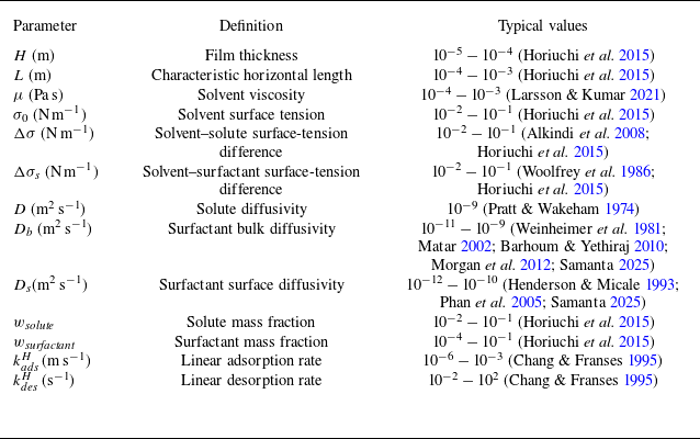
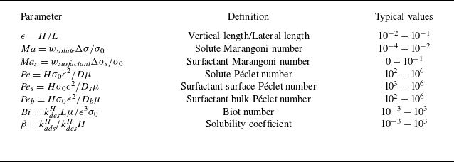


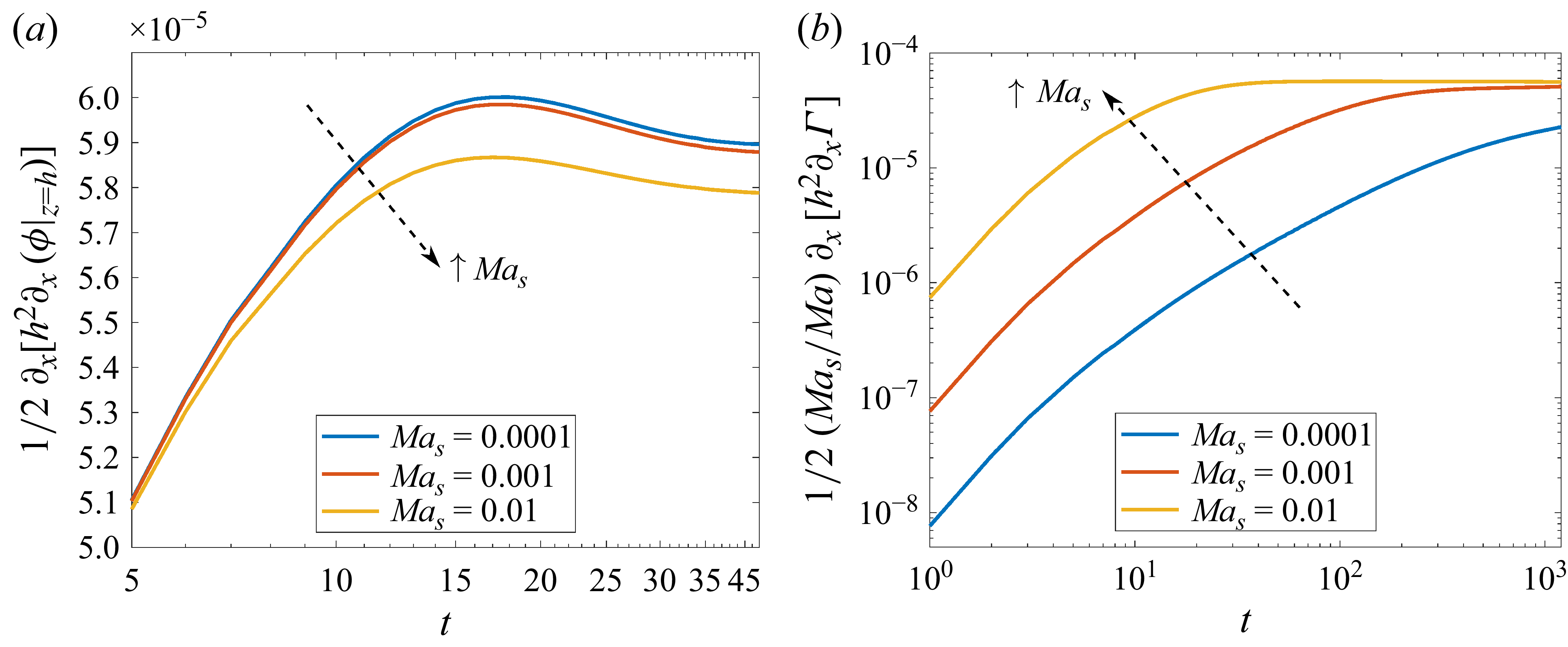


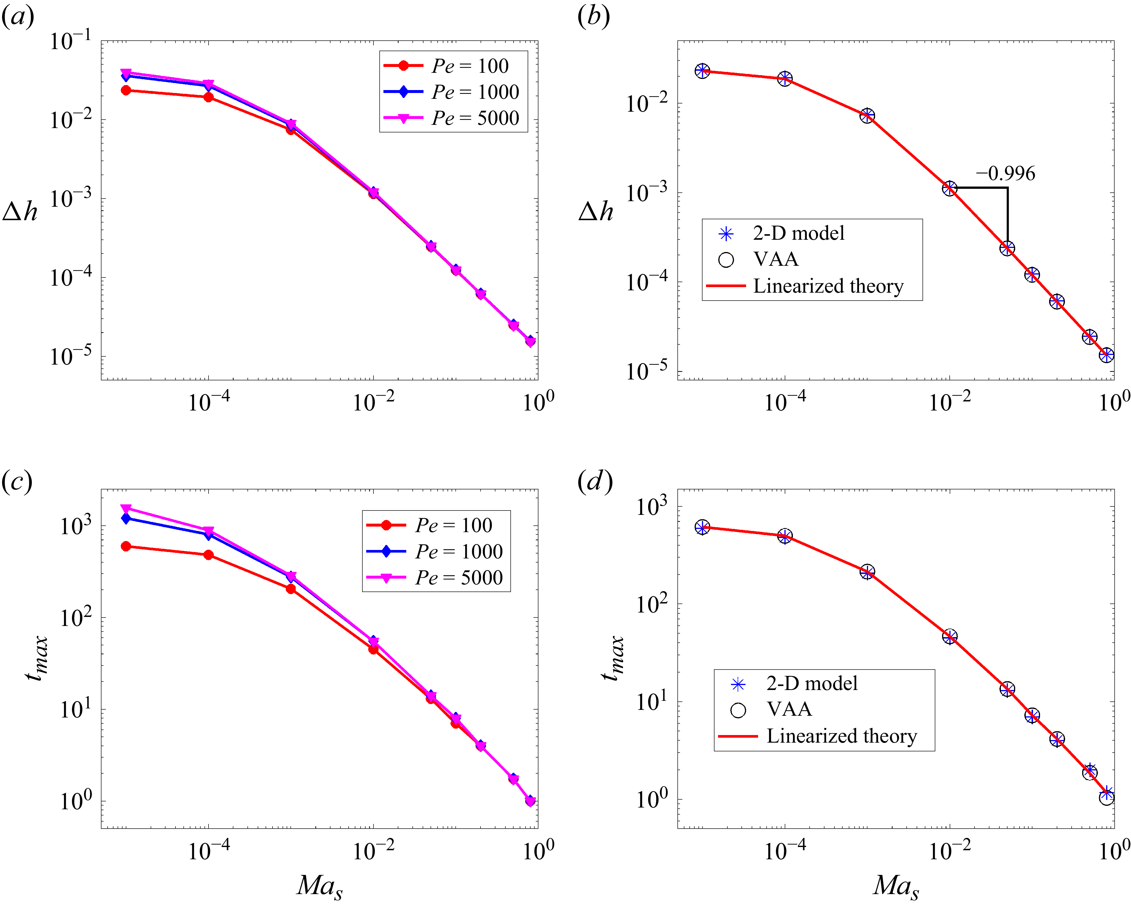


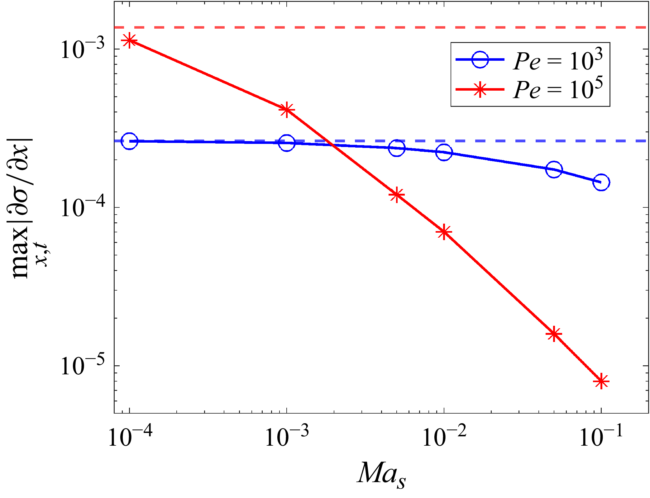


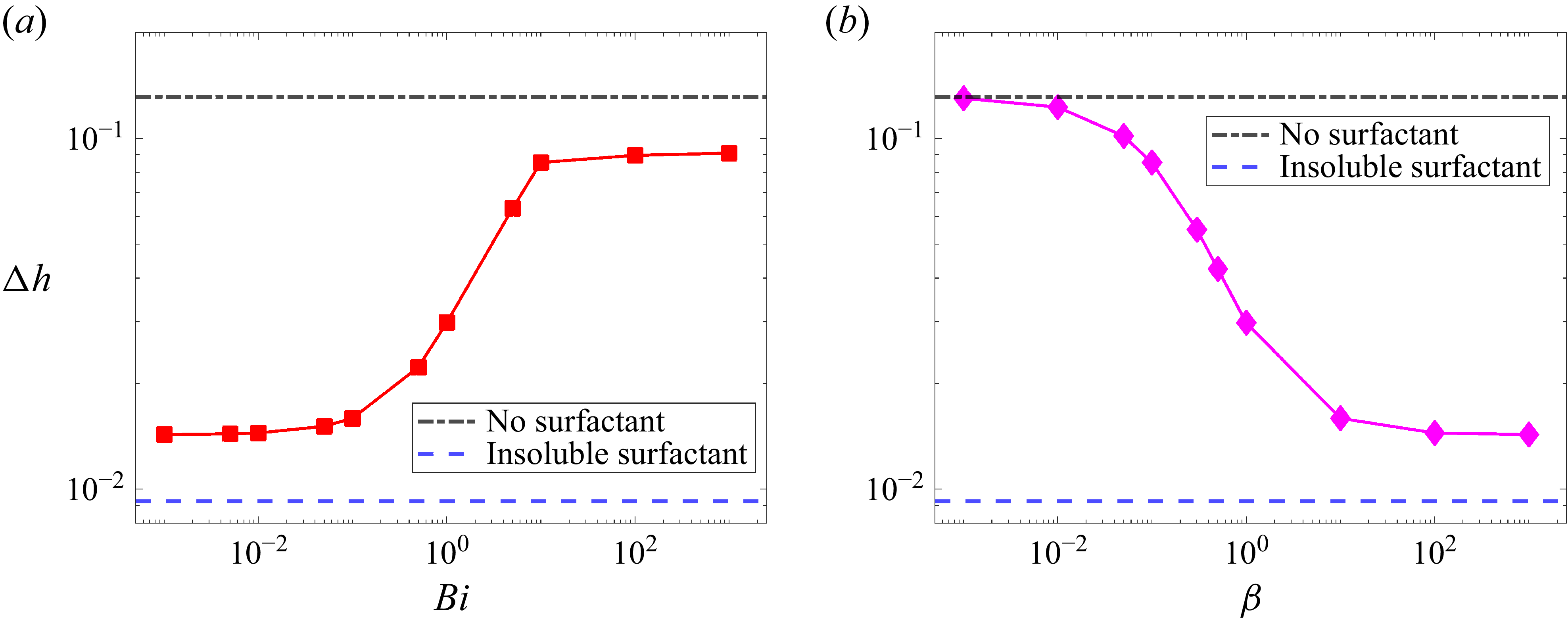


 Open access