


1 Introduction
For almost two decades after the introduction of Anosov flows in the early 1960s [Reference Anosov1, Reference Anosov2], the only known examples of Anosov flows on three-dimensional closed manifolds were based on either the suspension of Anosov diffeomorphisms of 2-torus or the geodesic flows on the unit tangent space of hyperbolic surfaces. All such examples are orbit equivalent to an algebraic volume-preserving flow by their natural construction and a lot of interesting properties of Anosov flows were derived, assuming the existence of such invariant volume forms. However, the first examples of Anosov flows, which are not orbit equivalent to a volume-preserving one, were constructed in 1980 by Franks and Williams [Reference Franks and Williams22]. Since then, understanding the relation between the existence of an invariant volume form and various aspects of Anosov dynamics has been sought from different viewpoints. In particular, from a topological viewpoint, such a property is associated with the transitivity of an Anosov flow [Reference Asaoka5] and from a measure theoretic viewpoint, they correspond to ergodic Anosov flows [Reference Anosov2, Reference Margulis38]. Moreover, many other dynamical aspects of such flows, including the regularity theoretical aspects, are well studied in the literature (for instance, see [Reference Hurder and Katok35, Reference Livšic and Sinaĭ37]).
Our goal in this paper, is to study the relation between the divergence of a flow and Anosovity in the context of a larger class of dynamics, namely the class of projectively Anosov flows, and using the notion of expansion rates of the invariant bundles. These quantities measure the infinitesimal change of the length of vectors in the stable and unstable directions, and facilitate a geometric understanding of Anosov flows. In particular, they play a significant role in the more recent contact and symplectic geometric theory of Anosov flows [Reference Hozoori33, Reference Mitsumatsu39, Reference Salmoiraghi45]. Therefore, our study provides new perspective on the class of volume preserving Anosov flows, in terms of those geometries.
It is worth mentioning that although projectively Anosov flows have been previously studied in various contexts, such as foliation theory [Reference Asaoka6, Reference Colin and Firmo15, Reference Eliashberg and Thurston18, Reference Noda40], Riemannian geometry [Reference Blair11, Reference Blair and Perrone12, Reference Hozoori34, Reference Perrone42], hyperbolic dynamics [Reference Arroyo and Hertz4, Reference Hirsch, Pugh and Shub31, Reference Pujals43, Reference Pujals and Sambarino44], and Reeb dynamics [Reference Hozoori32], their primary significance for us is that they serve as a bridge between Anosov dynamics and contact and symplectic geometry [Reference Mitsumatsu39] (see §2.2), eventually yielding a complete characterization of Anosov flows in terms of such geometries [Reference Hozoori33]. We remark that such flows are also referred to in the literature, using other names including conformally Anosov flows or flows with dominated splitting.
Assumptions. In this paper, unless stated otherwise, we assume that M is a closed connected oriented three manifold and X is a non-vanishing $C^{1+}$
vector field, that is, a
$C^{1+}$
vector field, that is, a $C^1$
vector field with Hölder continuous derivatives. We denote the
$C^1$
vector field with Hölder continuous derivatives. We denote the $C^{1+}$
flow generated by X by
$C^{1+}$
flow generated by X by $\phi ^t$
. It is noteworthy that there are other vector fields and flows involved in this paper, for instance the Reeb vector fields of Theorems 1.6 and 1.8, for which we do not assume any regularity and in fact, are often only
$\phi ^t$
. It is noteworthy that there are other vector fields and flows involved in this paper, for instance the Reeb vector fields of Theorems 1.6 and 1.8, for which we do not assume any regularity and in fact, are often only $C^0$
(also see Remark 5.2). We also assume the (projectively) Anosov flows to have transversely orientable invariant bundles. This is always achieved, possibly after lifting to a double cover of M. Moreover, we call any geometric quantity, which is differentiable in the direction of the flow, X-differentiable. The reader should consult [Reference Palis and De Melo41] for the basics of the theory of flows on manifolds, and [Reference Fisher and Hasselblatt19] for the fundamentals of hyperbolic flows.
$C^0$
(also see Remark 5.2). We also assume the (projectively) Anosov flows to have transversely orientable invariant bundles. This is always achieved, possibly after lifting to a double cover of M. Moreover, we call any geometric quantity, which is differentiable in the direction of the flow, X-differentiable. The reader should consult [Reference Palis and De Melo41] for the basics of the theory of flows on manifolds, and [Reference Fisher and Hasselblatt19] for the fundamentals of hyperbolic flows.
We begin our study with a natural description of the divergence of a projectively Anosov flow in terms of its associated expansion rates of the invariant bundles, encapsulated in the following two theorems.
Theorem 1.1. Let X be the generator of a projectively Anosov flow on M and $\Omega $
be some volume form which is X-differentiable. There exists a metric on M, such that
$\Omega $
be some volume form which is X-differentiable. There exists a metric on M, such that $\mathrm {div}_X\Omega =r_s+r_u$
, where
$\mathrm {div}_X\Omega =r_s+r_u$
, where $r_s$
and
$r_s$
and $r_u$
are the expansion rates of the stable and unstable directions, respectively, measured by such a metric.
$r_u$
are the expansion rates of the stable and unstable directions, respectively, measured by such a metric.
Theorem 1.2. Let X be the generator of a projectively Anosov flow and $\|.\|$
some X-differentiable norm on
$\|.\|$
some X-differentiable norm on $TM$
induced by a metric. Also, let
$TM$
induced by a metric. Also, let $r_s$
and
$r_s$
and $r_u$
be the expansion rates of the stable and unstable bundles, measured by
$r_u$
be the expansion rates of the stable and unstable bundles, measured by $\|.\|$
. Then:
$\|.\|$
. Then:
-
(a) there exists a volume form $\Omega $
on M, which is X-differentiable and
$\mathrm {div}_X\Omega =r_s+r_u$
;
$\Omega $
on M, which is X-differentiable and
$\mathrm {div}_X\Omega =r_s+r_u$
; -
(b) for any
$\epsilon>0$
, there exists a
$C^1$
volume form
$\Omega ^\epsilon \!$
, such that
$|\mathrm {div}_X\Omega ^\epsilon -(r_s+r_u)|<\epsilon $
.


Although the above description of the divergence is hardly surprising, it accommodates the use of such a relation from the viewpoint of differential and contact geometry. One immediate corollary is the following.
Corollary 1.3. Any projectively Anosov flow preserving some $C^0$
volume form is Anosov. In particular, any contact projectively Anosov flow (that is, when a projectively Anosov flow preserves a transverse contact structure) is Anosov.
$C^0$
volume form is Anosov. In particular, any contact projectively Anosov flow (that is, when a projectively Anosov flow preserves a transverse contact structure) is Anosov.
Although the above corollary is well known in the dynamical systems literature (for instance, see [Reference Araújo and Pacifico3]), it seems that this fact is unexpectedly left obscured in some other areas of research, most importantly when such flows appear in the Riemannian geometry literature. While contributing meaningfully to the related subjects, one can find many interesting results on the Riemannian geometry of contact projectively Anosov flows, ignoring that they are in fact Anosov (for instance, see [Reference Blair11, Reference Blair and Perrone12]).
It is well known that many important properties of (projectively) Anosov flows are independent of the norm involved in their definition. However, there are natural volume forms for such a setting, induced from the underlying contact structures of these flows (see §2.2). It turns out that we can characterize the Anosovity of a projectively Anosov flow in terms of the divergence of the flow being bounded by these volume forms in an appropriate sense (see Remark 4.1).
Theorem 1.4. Let X be the generating vector field for a projectively Anosov flow. Then, the following are equivalent:
-
(1) X is Anosov;
-
(2) there exists a positive contact form
$\alpha _+$
, such that for some
$\xi _-$
, the pair
$(\xi _-, \xi _+:=\ker {\alpha _+})$
is a supporting bi-contact structure and
$-\alpha _+ \wedge d\alpha _+<(\mathrm {div}_X\Omega ^{\alpha _+}) \Omega ^{\alpha _+} < \alpha _+\wedge d \alpha _+$
; -
(3) there exists a negative contact form
$\alpha _-$
, such that for some
$\xi _+$
, the pair
$(\xi _-:=\ker {\alpha _-},\xi _+)$
is a supporting bi-contact structure and
$\alpha _- \wedge d\alpha _-<(\mathrm {div}_X\Omega ^{\alpha _-})\Omega ^{\alpha _-} < -\alpha _-\wedge d \alpha _-.$


Remark 1.5. We remark that Theorems 1.1–1.4 and Corollary 1.3 above hold for any $C^1$
flow (without the assumption of Hölder continuity for its derivative). However, for Theorem 1.4 in that case, we would need the approximation techniques developed in [Reference Hozoori33] to deal with
$C^1$
flow (without the assumption of Hölder continuity for its derivative). However, for Theorem 1.4 in that case, we would need the approximation techniques developed in [Reference Hozoori33] to deal with $C^0$
weak stable and unstable bundles, since the Hölder continuity of the derivatives of the flow is needed to ensure such invariant plane fields are
$C^0$
weak stable and unstable bundles, since the Hölder continuity of the derivatives of the flow is needed to ensure such invariant plane fields are $C^1$
, which is used in the proof of Theorem 1.4 for simplicity.
$C^1$
, which is used in the proof of Theorem 1.4 for simplicity.
Using our description of the divergence of an Anosov flow, we next study the geometric consequences of the existence of an invariant volume form for an Anosov flow from various viewpoints. More precisely, Theorem 1.2 shows the symmetry of expansion and contraction in the unstable and stable directions, respectively, in the case of volume preserving Anosov flows and furthermore, thanks to the differentiability of the weak stable and unstable bundles in this case [Reference Hasselblatt30, Reference Hurder and Katok35], such symmetry behaves well when translating the metric description of Anosov flows to the contact geometric one. We study such symmetry from the view point of the theory of contact hyperbolas, Reeb dynamics, and Liouville geometry, giving various characterizations of volume preserving Anosov flows.
To begin with, we study volume preserving Anosov flows in terms of the theory of contact hyperbolas, developed by Perrone [Reference Perrone42] (see §5.1 for definitions), as an analog of the theory of contact circles by Geiges and Gonzalo [Reference Geiges and Gonzalo26, Reference Geiges and Gonzalo25]. Moreover, we will see that these conditions are, in fact, equivalent to a purely Reeb dynamical description of volume preserving Anosov flows.
Theorem 1.6. Let $\phi ^t$
be a projectively Anosov flow on M. Then, the following are equivalent:
$\phi ^t$
be a projectively Anosov flow on M. Then, the following are equivalent:
-
(1) the flow
$\phi ^t$
is a volume preserving Anosov flow; -
(2) there exists a supporting bi-contact structure
$(\xi _-,\xi _+)$
and contact forms
$\alpha _-$
and
$\alpha _+$
for
$\xi _-$
and
$\xi _+$
, respectively, such that
$(\alpha _-,\alpha _+)$
is a
$(-1)$
-Cartan structure; -
(3) there exists a supporting bi-contact structure
$(\xi _-,\xi _+)$
and Reeb vector fields
$R_{\alpha _-}$
and
$R_{\alpha _+}$
for
$\xi _-$
and
$\xi _+$
, respectively, such that
$R_{\alpha _-}\subset \xi _+$
and
$R_{\alpha _+}\subset \xi _-$
.


To the best of our knowledge, the only known examples of taut contact hyperbolas, except an explicit example constructed on $\mathbb {T}^3$
, are achieved using the symmetries of Lie manifolds, giving examples which are compatible with algebraic Anosov flows [Reference Perrone42]. However, Theorem 1.6 shows that we can also construct examples of taut contact hyperbolas on hyperbolic manifolds, thanks to the construction of an infinite family of contact Anosov flows on hyperbolic manifolds by Foulon and Hasselblatt [Reference Foulon and Hasselblatt21], as well as many examples on toroidal manifolds [Reference Béguin, Bonatti and Yu10]. We note that it is not known if any specific manifold can admit infinitely many distinct Anosov flows, while there are at most finitely many contact Anosov flows on any manifold up to orbit equivalence [Reference Barthelmé and Mann9]. This gives a partial answer to the classification problem posed in the final remark of [Reference Perrone42].
$\mathbb {T}^3$
, are achieved using the symmetries of Lie manifolds, giving examples which are compatible with algebraic Anosov flows [Reference Perrone42]. However, Theorem 1.6 shows that we can also construct examples of taut contact hyperbolas on hyperbolic manifolds, thanks to the construction of an infinite family of contact Anosov flows on hyperbolic manifolds by Foulon and Hasselblatt [Reference Foulon and Hasselblatt21], as well as many examples on toroidal manifolds [Reference Béguin, Bonatti and Yu10]. We note that it is not known if any specific manifold can admit infinitely many distinct Anosov flows, while there are at most finitely many contact Anosov flows on any manifold up to orbit equivalence [Reference Barthelmé and Mann9]. This gives a partial answer to the classification problem posed in the final remark of [Reference Perrone42].
Corollary 1.7. There exist infinitely many hyperbolic manifolds which admit a $(-1)$
-Cartan structure (and in particular, a taut contact hyperbola).
$(-1)$
-Cartan structure (and in particular, a taut contact hyperbola).
Moreover, we study volume preserving Anosov flows from the perspective of Liouville geometry. The construction of exact symplectic 4-manifold for a general Anosov 3-flow is done by the author in [Reference Hozoori33]. However, we observe that such construction is significantly simplified in the presence of an invariant volume form (the case previously studied by Mitsumatsu [Reference Mitsumatsu39]). In fact, after a canonical reparameterization of a volume preserving Anosov flow, we show that we can improve the relation between such flows and both the underlying Reeb dynamics of Theorem 1.6 as well as the Liouville geometry associated with the corresponding exact symplectic 4-manifold. We call such reparameterization the Liouville reparameterization of a volume preserving Anosov flow (see §5.2 for definitions).
Theorem 1.8. Let X be the generating vector field of a volume preserving Anosov flow. If $X_L$
is the generating vector field for the Liouville reparameterization of the flow, the following hold:
$X_L$
is the generating vector field for the Liouville reparameterization of the flow, the following hold:
-
(1) the flow generated by
$X_L$
preserves the transverse plane field
$\langle R_{\alpha _-},R_{\alpha _+} \rangle $
, where
$R_{\alpha _-}$
and
$R_{\alpha _+}$
are the Reeb vector fields of Theorem 1.6(2); -
(2) the pair
$(M,X_L)$
can be extended to a Liouville structure
$([-1,1]\times M,Y)$
, such that
$([-1,1]\times M,Y)|_{\{0\}\times M}=(M,X_L).$


Remark 1.9. It is important to note that in the above theorem, the plane field generated by $R_{\alpha _-}$
and
$R_{\alpha _-}$
and $R_{\alpha _+}$
is only continuous in the general case, and is
$R_{\alpha _+}$
is only continuous in the general case, and is $C^1$
if and only if the Liouville reparameterization generated by
$C^1$
if and only if the Liouville reparameterization generated by $X_L$
is contact or a suspension flow (this is done for
$X_L$
is contact or a suspension flow (this is done for $C^2$
flows in [Reference Foulon and Hasselblatt20], but a similar proof should work in the
$C^2$
flows in [Reference Foulon and Hasselblatt20], but a similar proof should work in the $C^{1+}$
category). In particular, this gives a bi-contact geometric way of distinguishing which Anosov flows are contact or a suspension flow. They are exactly the ones where the constructed Reeb vector fields
$C^{1+}$
category). In particular, this gives a bi-contact geometric way of distinguishing which Anosov flows are contact or a suspension flow. They are exactly the ones where the constructed Reeb vector fields $R_{\alpha _-}$
and
$R_{\alpha _-}$
and $R_{\alpha _+}$
in Theorem 1.8 are
$R_{\alpha _+}$
in Theorem 1.8 are $C^1$
.
$C^1$
.
At the end, we discuss the applications of our study to the surgery theory of Anosov flows. Surgery theory has been a very important part of the geometric theory of Anosov flows from the early days. Various Dehn-type surgery operations, including Handel and Thurston [Reference Handel and Thurston29], Goodman [Reference Goodman28], Fried [Reference Fried23], or Foulon and Hasselblatt [Reference Foulon and Hasselblatt21] surgeries, have helped the construction of new examples of Anosov flows, answering historically important questions. These include the first examples of Anosov flows on hyperbolic manifolds [Reference Goodman28], the construction of infinitely many contact Anosov flows on hyperbolic manifolds [Reference Foulon and Hasselblatt21], or the first (non-trivial) classification of Anosov flows on hyperbolic manifolds [Reference Yu49].
Recently, Salmoiraghi [Reference Salmoiraghi45, Reference Salmoiraghi46] has introduced two novel bi-contact geometric surgery operations of (projectively) Anosov flows, which contribute toward the contact geometric theory of Anosov flows (see [Reference Bowden, Bonatti and Potrie13, Reference Hozoori33, Reference Mitsumatsu39], for instance) and the related surgery theory, reconstructing the previously known surgery operations of Foulon and Hasselblatt and Handel and Thurston. These surgeries are applied in the neighborhood of a Legendrian-transverse knot, that is, a knot which is Legendrian (tangent) for one of the underlying contact structures in the supporting bi-contact and transverse for the other one (see §2.2). One of these surgery operations is done by cutting the manifold along an annulus tangent to the flow and the other is based on a transverse annulus. However, the relation to Goodman surgery, which is one of the most significant surgery operations on Anosov flows and is applied in the neighborhood of a periodic orbit of such a flow, relies on one condition. That requires being able to push a periodic orbit to a Legendrian-transverse knot. Salmoiraghi observes that this is possible for the unit tangent space of hyperbolic surfaces [Reference Salmoiraghi45] and, furthermore, shows that if such a condition is satisfied, the Goodman surgery can be reconstructed using the bi-contact surgery on a transverse annulus (in fact, he generalizes such an operation to projectively Anosov flows) [Reference Salmoiraghi46]. We show that such a condition can be satisfied for any Anosov flow by choosing a norm which yields constant divergence on a given periodic orbit of the flow, giving an affirmative answer to the question posed in [Reference Salmoiraghi45]. This takes us one step closer to a contact geometric surgery of Anosov flows, unifying the previously introduced operations (it is noteworthy that the equivalence of Fried and Goodman surgeries has been recently shown for transitive Anosov flows [Reference Shannon47], which is conjecturally true in the general case, and hence results in the use of the term Goodman–Fried surgery in the literature).
Theorem 1.10. Let $\phi ^t$
be an Anosov flow. Given any periodic orbit
$\phi ^t$
be an Anosov flow. Given any periodic orbit $\gamma _0$
, there exists a supporting bi-contact structure
$\gamma _0$
, there exists a supporting bi-contact structure $(\xi _-,\xi _+=\ker {\alpha _+})$
such that we have
$(\xi _-,\xi _+=\ker {\alpha _+})$
such that we have $R_{\alpha _+}\subset \xi _-$
in a regular neighborhood of
$R_{\alpha _+}\subset \xi _-$
in a regular neighborhood of $\gamma _0$
. Therefore, there exists an isotopy
$\gamma _0$
. Therefore, there exists an isotopy $\{\gamma _t\}_{t\in [0,1]}$
, which is supported in an arbitrary small neighborhood of
$\{\gamma _t\}_{t\in [0,1]}$
, which is supported in an arbitrary small neighborhood of $\gamma _0$
, and
$\gamma _0$
, and $\gamma _t$
is a Legendrian-transverse knot for any
$\gamma _t$
is a Legendrian-transverse knot for any $0<t\leq 1$
.
$0<t\leq 1$
.
Corollary 1.11. The bi-contact surgeries of Salmoiraghi [Reference Salmoiraghi45, Reference Salmoiraghi46] can be applied in an arbitrary small neighborhood of a periodic orbit of any Anosov flow. In particular, the bi-contact surgery of [Reference Salmoiraghi46] reconstructs the Goodman surgery.
In §2, we review some basic notions in Anosov dynamics and the expansion rates, as well as their connection to contact geometry. In §3, we describe the divergence of a (projectively) Anosov flow in terms of its associated expansion rates. In §4, we discuss some useful interplays between the contact geometry of Anosov flows and various volume forms on a three manifold, giving a contact geometric characterization of Anosovity based on divergence. In §5, we study the symmetries that the existence of an invariant volume form implies on the geometry of an Anosov flow from various viewpoints of the theory of contact hyperbolas, Reeb dynamics, and Liouville geometry. Finally, §6 is devoted to discussing the applications of our study to bi-contact surgeries.
2 Background
In this section, we bring the necessary background for the main results. First, we review some basics about Anosov flows in dimension 3 and their generalization to projectively Anosov flows. Then, we discuss the connection of such flows to contact geometry. This is not, by any means, a thorough treatment and one should consult references like [Reference Barthelmé8, Reference Fisher and Hasselblatt19, Reference Geiges24] on these subjects for a more complete perspective.
2.1 (Projectively) Anosov flows and the associated expansion rates
Anosov flows in dimension 3 are non-singular flows, whose action on the tangent space of the ambient manifold exhibits exponential expansion and contraction in two distinct transverse directions.
Definition 2.1. Let $\phi ^t$
be the flow generated by the non-vanishing
$\phi ^t$
be the flow generated by the non-vanishing $C^1$
vector field X. We call
$C^1$
vector field X. We call $\phi ^t$
Anosov if there exists a continuous invariant splitting
$\phi ^t$
Anosov if there exists a continuous invariant splitting $TM\simeq E^{ss} \oplus E^{uu} \oplus \langle X\rangle $
, such that for some positive constant C and a norm
$TM\simeq E^{ss} \oplus E^{uu} \oplus \langle X\rangle $
, such that for some positive constant C and a norm $\|.\|$
, we have
$\|.\|$
, we have
 $$ \begin{align*}\|\phi^t_*(u)\|\leq e^{-Ct}\|u\|\quad\text{and}\quad \|\phi^t_*(v)\|\geq e^{Ct}\|v\|\end{align*} $$
for any $u\in E^{ss}$
and
$u\in E^{ss}$
and $v\in E^{uu}$
. We call
$v\in E^{uu}$
. We call $E^{ss}$
and
$E^{ss}$
and $E^{uu}$
strong stable and unstable directions, respectively.
$E^{uu}$
strong stable and unstable directions, respectively.
The classical examples of such flows are the geodesic flows on the unit tangent bundle of hyperbolic surfaces and the suspension of Anosov diffeomorphisms of torus. However, various surgery operations on Anosov flows have yielded many more examples, including infinitely many examples on hyperbolic manifolds. These include surgeries of Handel and Thurston [Reference Handel and Thurston29], Fried [Reference Fried23], Goodman [Reference Goodman28], Foulon and Hassleblatt [Reference Foulon and Hasselblatt21], and more recently, the bi-contact geometric surgeries introduced by Salmoiraghi [Reference Salmoiraghi45, Reference Salmoiraghi46], which manage to reproduce, up to orbit equivalence, the previous operations in many cases.
Remark 2.2. We remark that the Anosovity of a non-singular flow can be determined by its action on the normal bundle of the direction of the flow. More precisely, a flow $\phi ^t$
, generated by the non-vanishing vector field X, induces a flow on
$\phi ^t$
, generated by the non-vanishing vector field X, induces a flow on $TM/\langle X \rangle $
via
$TM/\langle X \rangle $
via $\pi :TM\rightarrow TM/\langle X \rangle $
, usually called the induced Poincaré linear flow. It is a classical result in dynamical systems by Doering [Reference Doering17] that a flow is Anosov if and only if the induced Poincaré linear flow admits a hyperbolic splitting. That is, there exists a continuous splitting of the normal bundle
$\pi :TM\rightarrow TM/\langle X \rangle $
, usually called the induced Poincaré linear flow. It is a classical result in dynamical systems by Doering [Reference Doering17] that a flow is Anosov if and only if the induced Poincaré linear flow admits a hyperbolic splitting. That is, there exists a continuous splitting of the normal bundle $TM/\langle X\rangle \simeq E^s \oplus E^u$
, which is invariant under the induced Poincaré linear flow and with respect to some norm, the action of such a flow on
$TM/\langle X\rangle \simeq E^s \oplus E^u$
, which is invariant under the induced Poincaré linear flow and with respect to some norm, the action of such a flow on $E^u$
and
$E^u$
and $E^s$
is exponentially expanding and contracting, respectively.
$E^s$
is exponentially expanding and contracting, respectively.
One important generalization of Anosov flows, which bridges Anosov dynamics to contact geometry, is the following.
Definition 2.3. Let $\tilde {\phi }^t$
be the Poincaré linear flow as in Remark 2.2. We call
$\tilde {\phi }^t$
be the Poincaré linear flow as in Remark 2.2. We call $\phi ^t$
projectively Anosov if there exists a continuous invariant splitting
$\phi ^t$
projectively Anosov if there exists a continuous invariant splitting $TM/\langle X\rangle \simeq E^{s} \oplus E^{u}$
, such that for some positive constant C and a norm
$TM/\langle X\rangle \simeq E^{s} \oplus E^{u}$
, such that for some positive constant C and a norm $\|.\|$
, we have
$\|.\|$
, we have
 $$ \begin{align*}\|\tilde{\phi}^t_*(v)\|/\|\tilde{\phi}^t_*(u)\|\leq e^{Ct}\|v\|/\|u\|\end{align*} $$
for any $u\in E^{s}$
and
$u\in E^{s}$
and $v\in E^{u}$
. We call
$v\in E^{u}$
. We call $E^s$
and
$E^s$
and $E^u$
stable and unstable directions, respectively.
$E^u$
stable and unstable directions, respectively.
In other words, a flow is projectively Anosov if its induced Poincaré linear flow admits a dominated splitting. That is, a continuous and invariant splitting into two line bundles on which the action of the flow is relatively expanding in one direction with respect to the other.
Abusing notation, we also refer to $\pi ^{-1}(E^s)$
and
$\pi ^{-1}(E^s)$
and $\pi ^{-1}(E^u)$
, which are a priori
$\pi ^{-1}(E^u)$
, which are a priori $C^0$
two-dimensional sub bundles of
$C^0$
two-dimensional sub bundles of $TM$
, by
$TM$
, by $E^s$
and
$E^s$
and $E^u$
, respectively, and call them the weak stable and unstable bundles, respectively (see Remark 2.5).
$E^u$
, respectively, and call them the weak stable and unstable bundles, respectively (see Remark 2.5).
In the case where a projectively Anosov flow is Anosov, the weak stable and unstable bundles are known to be $C^1$
[Reference Hasselblatt30]. It is worth mentioning that that unlike the Anosov case (as discussed in Remark 2.2), in the case of projectively Anosov flows, the splitting of the normal bundle
$C^1$
[Reference Hasselblatt30]. It is worth mentioning that that unlike the Anosov case (as discussed in Remark 2.2), in the case of projectively Anosov flows, the splitting of the normal bundle $TM/\langle X\rangle $
cannot necessarily be lifted to the tangent space
$TM/\langle X\rangle $
cannot necessarily be lifted to the tangent space $TM$
[Reference Noda40].
$TM$
[Reference Noda40].
Although it is not a priori obvious if such a class of dynamics is strictly larger than the class of Anosov flows, we know that projectively Anosov flows are abundant. See [Reference Eliashberg and Thurston18, Reference Mitsumatsu39] for examples on torus bundles, [Reference Bowden, Bonatti and Potrie13] for non-Anosov examples on hyperbolic manifolds, and [Reference Asaoka, Dufraine and Noda7] for a more general construction.
To build the bridge from the above definitions to the world of differential and contact geometry, it is very useful for us to measure the infinitesimal expansion or contraction of the length of vectors in the invariant bundles. Note that without loss of generality, we can assume the norm involved in the definition of (projectively) Anosov flows is $C^\infty $
.
$C^\infty $
.
Definition 2.4. Using the above notation and considering $TM/\langle X\rangle \simeq E^{s} \oplus E^{u}$
, let
$TM/\langle X\rangle \simeq E^{s} \oplus E^{u}$
, let ${\tilde {e}_s\in E^s}$
and
${\tilde {e}_s\in E^s}$
and $\tilde {e}_u\in E^u$
be the unit vectors with respect to some X-differentiable norm
$\tilde {e}_u\in E^u$
be the unit vectors with respect to some X-differentiable norm $\|.\|$
on
$\|.\|$
on $TM/\langle X\rangle $
. We call
$TM/\langle X\rangle $
. We call
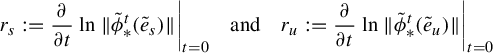 $$ \begin{align*}r_s:=\frac{\partial}{\partial t} \ln{\|\tilde{\phi}_*^t (\tilde{e}_s)\|}\bigg|_{t=0}\quad\text{and} \quad r_u:=\frac{\partial}{\partial t} \ln{\|\tilde{\phi}_*^t (\tilde{e}_u)\|}\bigg|_{t=0}\end{align*} $$
the expansion rates of the stable and unstable directions, respectively, with respect to $\|.\|$
.
$\|.\|$
.
We remark that similar notions have been previously used in the study of various aspects of Anosov flows [Reference Coles and Sharp14, Reference Hasselblatt30, Reference Simić48].
Remark 2.5. Note that the norm used in the definition of expansion rates is defined on the normal bundle $TM/\langle X\rangle $
. However, it is easy to describe these quantities based on the tangent bundle
$TM/\langle X\rangle $
. However, it is easy to describe these quantities based on the tangent bundle $TM$
. First, given a norm on
$TM$
. First, given a norm on $TM/\langle X\rangle $
, consider some metric on this vector bundle, which induces the norm. Notice that given any transverse
$TM/\langle X\rangle $
, consider some metric on this vector bundle, which induces the norm. Notice that given any transverse $C^1$
plane field
$C^1$
plane field $\eta $
, there exists a natural isomorphism
$\eta $
, there exists a natural isomorphism $\eta \simeq TM/\langle X\rangle $
via the projection
$\eta \simeq TM/\langle X\rangle $
via the projection $\pi :TM\rightarrow \eta \simeq TM/\langle X\rangle $
. Therefore, a Riemannian metric on
$\pi :TM\rightarrow \eta \simeq TM/\langle X\rangle $
. Therefore, a Riemannian metric on $TM/\langle X\rangle $
induces a Riemannian metric on
$TM/\langle X\rangle $
induces a Riemannian metric on $\eta $
, which can be naturally extended to
$\eta $
, which can be naturally extended to $TM$
by letting
$TM$
by letting $\|X\|=1$
and
$\|X\|=1$
and $X\perp \eta $
, where
$X\perp \eta $
, where $\|.\|$
is the norm on
$\|.\|$
is the norm on $TM$
induced from such a metric. If
$TM$
induced from such a metric. If $\tilde {e}_s \in E^s \subset TM/\langle X\rangle $
and
$\tilde {e}_s \in E^s \subset TM/\langle X\rangle $
and $\tilde {e}_u\in E^u\subset TM/\langle X\rangle $
are the unit vector fields, their image
$\tilde {e}_u\in E^u\subset TM/\langle X\rangle $
are the unit vector fields, their image $e_s\in \pi ^{-1}(E^s)\cap \eta $
and
$e_s\in \pi ^{-1}(E^s)\cap \eta $
and $e_u\in \pi ^{-1}(E^u)\cap \eta $
, under the isomorphism, are unit vector fields with respect to the norm induced on
$e_u\in \pi ^{-1}(E^u)\cap \eta $
, under the isomorphism, are unit vector fields with respect to the norm induced on $TM$
. It is easy to compute
$TM$
. It is easy to compute
 $$ \begin{align*}\mathcal{L}_X e_s=-r_se_s +q_s X\quad\text{and}\quad \mathcal{L}_X e_u=-r_ue_u +q_u X,\end{align*} $$
where $q_s$
and
$q_s$
and $q_u$
are real functions, depending on our choice of
$q_u$
are real functions, depending on our choice of $\eta $
. Note that we will have
$\eta $
. Note that we will have $q_s=q_u=0$
when
$q_s=q_u=0$
when $\eta $
is preserved by X (see §3 of [Reference Hozoori33] for a more thorough discussion). Since we are assuming
$\eta $
is preserved by X (see §3 of [Reference Hozoori33] for a more thorough discussion). Since we are assuming $\eta $
to be
$\eta $
to be $C^1$
, this only happens for an Anosov flow when it is contact or a suspension flow [Reference Foulon and Hasselblatt20].
$C^1$
, this only happens for an Anosov flow when it is contact or a suspension flow [Reference Foulon and Hasselblatt20].
Note that this remark also justifies the abuse of notation we adopted in the beginning of this section, that is, referring to $\pi ^{-1}(E^s)$
by
$\pi ^{-1}(E^s)$
by $E^s$
(and similarly for
$E^s$
(and similarly for $E^u$
). To be clearer, the correspondence between the metrics on
$E^u$
). To be clearer, the correspondence between the metrics on $TM$
and
$TM$
and $TM/\langle X\rangle $
discussed above allows us to talk about the unit vector
$TM/\langle X\rangle $
discussed above allows us to talk about the unit vector $e_s\in E^s$
and, therefore, the expansion rate of the stable direction unambiguously, whether we consider
$e_s\in E^s$
and, therefore, the expansion rate of the stable direction unambiguously, whether we consider $E^s\subset TM$
or
$E^s\subset TM$
or $E^s \subset TM/\langle X \rangle $
. The same holds for
$E^s \subset TM/\langle X \rangle $
. The same holds for $e_u\in E^u$
and the expansion rate of the unstable direction.
$e_u\in E^u$
and the expansion rate of the unstable direction.
Remark 2.6. Alternatively, one can characterize the expansion rates in terms of differential forms. Consider a metric on $TM/\langle X \rangle $
and define
$TM/\langle X \rangle $
and define $\tilde {\alpha _s}$
as a differential form on
$\tilde {\alpha _s}$
as a differential form on $TM/\langle X \rangle $
by letting
$TM/\langle X \rangle $
by letting $\ker {\tilde {\alpha _s}}=E^u\subset TM/\langle X \rangle $
and
$\ker {\tilde {\alpha _s}}=E^u\subset TM/\langle X \rangle $
and $\tilde {\alpha _s}(\tilde {e}_s)=1$
, where
$\tilde {\alpha _s}(\tilde {e}_s)=1$
, where $\tilde {e}_s\in E^s\subset TM/\langle X \rangle $
is a unit vector field with respect to the chosen metric. Similarly, define
$\tilde {e}_s\in E^s\subset TM/\langle X \rangle $
is a unit vector field with respect to the chosen metric. Similarly, define $\tilde {\alpha }_u$
and easily compute
$\tilde {\alpha }_u$
and easily compute
 $$ \begin{align*}\mathcal{L}_X \tilde{\alpha}_s=r_s\tilde{\alpha}_s\quad\text{and}\quad \mathcal{L}_X \tilde{\alpha}_u=r_u\tilde{\alpha}_u,\end{align*} $$
where $r_s$
and
$r_s$
and $r_u$
are the expansion rates of the stable and unstable directions with respect to such a metric.
$r_u$
are the expansion rates of the stable and unstable directions with respect to such a metric.
As we will see in the remainder of the paper, it is usually desirable to work with differential forms on $TM$
. Therefore, we can define
$TM$
. Therefore, we can define $\alpha _s:=\pi ^*\tilde {\alpha }_s$
and
$\alpha _s:=\pi ^*\tilde {\alpha }_s$
and $\alpha _u:=\pi ^*\tilde {\alpha }_u$
, where
$\alpha _u:=\pi ^*\tilde {\alpha }_u$
, where $\pi :TM\rightarrow TM/\langle X\rangle \simeq \eta $
is the natural projection, and note that
$\pi :TM\rightarrow TM/\langle X\rangle \simeq \eta $
is the natural projection, and note that
 $$ \begin{align*}\mathcal{L}_X \alpha_s=r_s\alpha_s\quad\text{and}\quad \mathcal{L}_X \alpha_u=r_u\alpha_u.\end{align*} $$
In fact, the above expressions can be taken as the definition of the expansion rates $r_s$
and
$r_s$
and $r_u$
. More precisely, if we take the unit vector fields
$r_u$
. More precisely, if we take the unit vector fields $e_s\in E^s\cap \eta \subset TM$
and
$e_s\in E^s\cap \eta \subset TM$
and $e_u\in E^u\cap \eta \subset TM$
, induced after choosing a transverse plane field
$e_u\in E^u\cap \eta \subset TM$
, induced after choosing a transverse plane field $\eta $
as in Remark 2.5, and define the differential form
$\eta $
as in Remark 2.5, and define the differential form $\alpha _s$
by letting
$\alpha _s$
by letting $\ker {\alpha _s}=E^u\oplus \langle X\rangle $
and
$\ker {\alpha _s}=E^u\oplus \langle X\rangle $
and $\alpha _s(e_s)=1$
, this matches the definition above. The same holds for
$\alpha _s(e_s)=1$
, this matches the definition above. The same holds for $\alpha _u$
. This means that, as in Remark 2.5, the choice of the transverse plane field
$\alpha _u$
. This means that, as in Remark 2.5, the choice of the transverse plane field $\eta $
does not affect the geometry of expansion in terms of differential forms on
$\eta $
does not affect the geometry of expansion in terms of differential forms on $TM$
.
$TM$
.
Not surprisingly, the (relative) exponential expansion for (projectively) Anosov flows can be easily characterized in terms of such expansion rates (see [Reference Hozoori33] for more details and proofs).
Proposition 2.7. Let X be a projectively Anosov vector field and $r_s$
and
$r_s$
and $r_u$
, the expansion rates of stable and unstable directions, respectively, with respect to any Riemannian metric satisfying the metric condition of Definition 2.3, which is X-differentiable. Then,
$r_u$
, the expansion rates of stable and unstable directions, respectively, with respect to any Riemannian metric satisfying the metric condition of Definition 2.3, which is X-differentiable. Then,
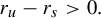 $$ \begin{align*}r_u-r_s>0.\end{align*} $$
While Proposition 2.7 expresses the relative expansion in the unstable direction with respect to the stable direction, the following proposition realizes when we have absolute expansion and contraction in those directions, which by Doering’s result [Reference Doering17] yields Anosovity (see Remark 2.2).
Proposition 2.8. Let X be a projectively Anosov vector field and $r_s$
and
$r_s$
and $r_u$
. Then X is Anosov if and only if, with respect to some Riemannian metric, we have
$r_u$
. Then X is Anosov if and only if, with respect to some Riemannian metric, we have
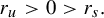 $$ \begin{align*}r_u>0>r_s.\end{align*} $$
2.2 Relation to (bi-)contact geometry
Recall that a $C^1$
1-form
$C^1$
1-form $\alpha $
is a contact form on M if
$\alpha $
is a contact form on M if $\alpha \wedge d\alpha $
is a non-vanishing volume form on M. If
$\alpha \wedge d\alpha $
is a non-vanishing volume form on M. If $\alpha \wedge d\alpha>0$
(compared to the orientation on M), we call
$\alpha \wedge d\alpha>0$
(compared to the orientation on M), we call $\alpha $
a positive contact form and otherwise, a negative one. We call the
$\alpha $
a positive contact form and otherwise, a negative one. We call the $C^1$
plane field
$C^1$
plane field $\xi :=\ker {\alpha }$
a (positive or negative) contact structure on M. Notice that by the Frobenuis theorem, contact structures can be thought of as maximally non-integrable
$\xi :=\ker {\alpha }$
a (positive or negative) contact structure on M. Notice that by the Frobenuis theorem, contact structures can be thought of as maximally non-integrable $C^1$
plane fields, that is, the extreme opposite of foliations.
$C^1$
plane fields, that is, the extreme opposite of foliations.
For example, $\xi _{std}:=\ker {dz-ydx}$
(
$\xi _{std}:=\ker {dz-ydx}$
( $\xi _{std}:=\ker {dz+ydx}$
) is called the standard positive (negative) contact structure on
$\xi _{std}:=\ker {dz+ydx}$
) is called the standard positive (negative) contact structure on $\mathbb {R}^3$
, while
$\mathbb {R}^3$
, while $\xi _n:=\ker {\{\cos {2\pi n z}dx-\sin {2\pi n} dy \}}$
on
$\xi _n:=\ker {\{\cos {2\pi n z}dx-\sin {2\pi n} dy \}}$
on $\mathbb {T}^3\,{=}\,\mathbb {R}^3/\mathbb {Z}^3$
gives an infinite family of distinct positive (negative) contact structures, when
$\mathbb {T}^3\,{=}\,\mathbb {R}^3/\mathbb {Z}^3$
gives an infinite family of distinct positive (negative) contact structures, when $n\in \mathbb {Z}>0$
(
$n\in \mathbb {Z}>0$
( $n<0$
).
$n<0$
).
Although we do not go toward the topological aspects of contact structures in this paper, it is worth mentioning that positive (negative) contact structures do not have any local invariant, thanks to the Darboux theorem that states that any two positive (negative) contact structures are locally contactomorphic (that is, locally look like the standard model on $\mathbb {R}^3$
). Furthermore, Gray’s theorem shows that any homotopy of a contact structure through contact structures is induced by an isotopy of the ambient manifold.
$\mathbb {R}^3$
). Furthermore, Gray’s theorem shows that any homotopy of a contact structure through contact structures is induced by an isotopy of the ambient manifold.
Associated to any contact structure, there is an important class of flows, which we will use in this paper. Given any contact form $\alpha $
for a contact structure
$\alpha $
for a contact structure $\xi :=\ker {\alpha }$
, there exists a unique vector field
$\xi :=\ker {\alpha }$
, there exists a unique vector field $R_{\alpha }$
, satisfying
$R_{\alpha }$
, satisfying
 $$ \begin{align*}d\alpha(R_{\alpha},.)=0\quad\text{and}\quad \alpha(R_\alpha)=1.\end{align*} $$
Such a vector field is called a Reeb vector field and it is easy to check $\mathcal {L}_{R_\alpha }\alpha =0$
. This implies
$\mathcal {L}_{R_\alpha }\alpha =0$
. This implies $\mathcal {L}_{R_\alpha }\alpha \wedge d\alpha =0$
. In particular, Reeb vector fields are volume preserving. Furthermore, Reeb vector fields preserve
$\mathcal {L}_{R_\alpha }\alpha \wedge d\alpha =0$
. In particular, Reeb vector fields are volume preserving. Furthermore, Reeb vector fields preserve $\xi $
, and are transverse to the underlying contact structure. It is easy to observe that conversely, given a contact structure, any transverse vector field preserving the contact structure
$\xi $
, and are transverse to the underlying contact structure. It is easy to observe that conversely, given a contact structure, any transverse vector field preserving the contact structure $\xi $
is a Reeb vector field for an appropriate choice of contact form.
$\xi $
is a Reeb vector field for an appropriate choice of contact form.
A natural and well-studied interplay of contact geometry and Anosov dynamics happens when a Reeb vector field is Anosov, that is, the case of contact Anosov flows (see for instance [Reference Foulon and Hasselblatt21]). However, in this paper, we are interested in a more general relation between the two theories, thanks to the following proposition, first observed by Mitsumatsu [Reference Mitsumatsu39] and Eliashberg and Thurston [Reference Eliashberg and Thurston18], which characterizes projectively Anosov flows in terms of contact geometry. We remind the reader that, as mentioned in the introduction of the paper, we are assuming the underlying manifold to be oriented and the invariant bundles for the projectively Anosov flows to be transversely orientable.
Proposition 2.9. Let X be a non-vanishing $C^1$
vector field on M. Then, X generates a projectively Anosov flow if and only if there exist positive and negative contact structures,
$C^1$
vector field on M. Then, X generates a projectively Anosov flow if and only if there exist positive and negative contact structures, $\xi _+$
and
$\xi _+$
and $\xi _-$
, respectively, which are transverse and
$\xi _-$
, respectively, which are transverse and $X\subset \xi _+ \cap \xi _-$
.
$X\subset \xi _+ \cap \xi _-$
.
In other words, considering a projectively Anosov flow, the bi-sectors of $E^s$
and
$E^s$
and $E^u$
can be seen to be a pair of positive and negative contact structures, possibly after a perturbation to make them
$E^u$
can be seen to be a pair of positive and negative contact structures, possibly after a perturbation to make them $C^1$
. And conversely, any vector field directing the intersection of such transverse pair is projectively Anosov.
$C^1$
. And conversely, any vector field directing the intersection of such transverse pair is projectively Anosov.
We note that the above proposition also shows that the (periodic) orbits of a projectively Anosov flows are Legendrian (knots), that is, tangent, for both of the underlying contact structures.
Using Proposition 2.9, we can easily give examples of non-Anosov projectively Anosov flows. For instance, $(\xi _m:=\ker {\{dz+\epsilon (\cos {2\pi m z}dx-\sin {2\pi m} dy)\}},\xi _n:=\ker {\{dz+\epsilon '(\cos {2\pi n z}dx-\sin {2\pi n} dy) \}})$
is a pair of positive and negative transverse contact structures, whenever
$(\xi _m:=\ker {\{dz+\epsilon (\cos {2\pi m z}dx-\sin {2\pi m} dy)\}},\xi _n:=\ker {\{dz+\epsilon '(\cos {2\pi n z}dx-\sin {2\pi n} dy) \}})$
is a pair of positive and negative transverse contact structures, whenever $m<0<n$
are integers and
$m<0<n$
are integers and $\epsilon \neq \epsilon '$
. Therefore, any flow, whose generating vector field lies in the intersection
$\epsilon \neq \epsilon '$
. Therefore, any flow, whose generating vector field lies in the intersection $\xi _m\cap \xi _n$
, is a projectively Anosov flow on
$\xi _m\cap \xi _n$
, is a projectively Anosov flow on $\mathbb {T}^3=\mathbb {R}^3/\mathbb {Z}^3$
by Proposition 2.9. Note that there are no Anosov flows on
$\mathbb {T}^3=\mathbb {R}^3/\mathbb {Z}^3$
by Proposition 2.9. Note that there are no Anosov flows on $\mathbb {T}^3$
.
$\mathbb {T}^3$
.
We call such pair of transverse negative and positive contact structures $(\xi _-,\xi _+)$
a bi-contact structure, supporting the underlying projectively Anosov flow. It turns out that by enriching a bi-contact structure with additional contact geometric structures, one can also characterize Anosov flows purely in terms of contact geometry [Reference Hozoori33].
$(\xi _-,\xi _+)$
a bi-contact structure, supporting the underlying projectively Anosov flow. It turns out that by enriching a bi-contact structure with additional contact geometric structures, one can also characterize Anosov flows purely in terms of contact geometry [Reference Hozoori33].
3 Divergence and the expansion rates
In this section, we show that the divergence of a projectively Anosov flow with respect to the (a priori $C^0$
) volume form, which is induced from any norm satisfying the relevant definition, can naturally be characterized in terms of the expansion rates of the stable and unstable directions. We then give approximation results for volume forms with higher regularity.
$C^0$
) volume form, which is induced from any norm satisfying the relevant definition, can naturally be characterized in terms of the expansion rates of the stable and unstable directions. We then give approximation results for volume forms with higher regularity.
Theorem 3.1. Let X be the generator of a projectively Anosov flow on M and $\Omega $
be some volume form which is X-differentiable. There exists a metric on M, such that
$\Omega $
be some volume form which is X-differentiable. There exists a metric on M, such that $\mathrm {div}_X\Omega =r_s+r_u$
, where
$\mathrm {div}_X\Omega =r_s+r_u$
, where $r_s$
and
$r_s$
and $r_u$
are the expansion rates of the stable and unstable directions, respectively, measured by the metric.
$r_u$
are the expansion rates of the stable and unstable directions, respectively, measured by the metric.
Proof. Choose a $C^\infty $
transverse plane field
$C^\infty $
transverse plane field $\eta $
and let
$\eta $
and let $\alpha _X$
be a
$\alpha _X$
be a $C^1\!$
1-form such that
$C^1\!$
1-form such that ${\alpha _X(\eta )=0}$
and
${\alpha _X(\eta )=0}$
and $\alpha _X(X)=1$
. Furthermore, choose some contact form
$\alpha _X(X)=1$
. Furthermore, choose some contact form $\tilde {\alpha }_+$
, so that
$\tilde {\alpha }_+$
, so that $(\xi _-,\xi _+:=\ker {\tilde {\alpha }_+})$
is a supporting bi-contact structure for X, for some negative contact structure
$(\xi _-,\xi _+:=\ker {\tilde {\alpha }_+})$
is a supporting bi-contact structure for X, for some negative contact structure $\xi _-$
.
$\xi _-$
.
We can write $\tilde {\alpha }_+=\tilde {\alpha }_u-\tilde {\alpha }_s$
, where
$\tilde {\alpha }_+=\tilde {\alpha }_u-\tilde {\alpha }_s$
, where $\tilde {\alpha }_u|_{E^s}=\tilde {\alpha }_s|_{E^u}=0$
. Notice that
$\tilde {\alpha }_u|_{E^s}=\tilde {\alpha }_s|_{E^u}=0$
. Notice that $\tilde {\alpha }_u$
and
$\tilde {\alpha }_u$
and $\tilde {\alpha }_s$
are
$\tilde {\alpha }_s$
are $C^0$
1-forms, which are X-differentiable, since
$C^0$
1-forms, which are X-differentiable, since $\tilde {\alpha }_+$
is
$\tilde {\alpha }_+$
is $C^1$
and the projection resulting in such decomposition is X-differentiable.
$C^1$
and the projection resulting in such decomposition is X-differentiable.
Since $\tilde {\alpha }_s \wedge \tilde {\alpha }_u \wedge \alpha _X$
is a volume form on M, there exists a positive function
$\tilde {\alpha }_s \wedge \tilde {\alpha }_u \wedge \alpha _X$
is a volume form on M, there exists a positive function $f:M\rightarrow ~\mathbb {R}^{+}$
, such that
$f:M\rightarrow ~\mathbb {R}^{+}$
, such that $|\Omega |=|\alpha _s \wedge \alpha _u \wedge \alpha _X|$
, where
$|\Omega |=|\alpha _s \wedge \alpha _u \wedge \alpha _X|$
, where $\alpha _s=f\tilde {\alpha }_s$
and
$\alpha _s=f\tilde {\alpha }_s$
and $\alpha _u=f\tilde {\alpha }_u$
.
$\alpha _u=f\tilde {\alpha }_u$
.
Finally, we can define the norm $\|.\|$
with
$\|.\|$
with $\|X\|=\|e_s\|=\|e_u\|=1$
, where
$\|X\|=\|e_s\|=\|e_u\|=1$
, where ${e_s\in E^s\cap \eta }$
,
${e_s\in E^s\cap \eta }$
, $e_u\in E^u\cap \eta $
,
$e_u\in E^u\cap \eta $
, $|\alpha _s(e_s)|=|\alpha _u(e_u)|=1$
, and
$|\alpha _s(e_s)|=|\alpha _u(e_u)|=1$
, and $(e_s,e_u,X)$
is a an oriented basis for
$(e_s,e_u,X)$
is a an oriented basis for $TM$
. Notice that by construction,
$TM$
. Notice that by construction, $\|.\|$
is X-differentiable.
$\|.\|$
is X-differentiable.
Letting $r_s$
and
$r_s$
and $r_u$
be the expansion rates of the stable and unstable directions, respectively, we can compute
$r_u$
be the expansion rates of the stable and unstable directions, respectively, we can compute
 $$ \begin{align*}(\mathcal{L}_X\Omega)\ (e_s,e_u,X)=-\Omega([X,e_s],e_u,X)-\Omega(e_s,[X,e_u],X)=(r_s+r_u)\ \Omega(e_s,e_u,X),\end{align*} $$
completing the proof.
Corollary 3.2. Any projectively Anosov flow preserving some $C^0$
volume form is Anosov. In particular, any contact projectively Anosov flow is Anosov.
$C^0$
volume form is Anosov. In particular, any contact projectively Anosov flow is Anosov.
Proof. Note that any preserved $C^0$
volume form is X-differentiable (
$C^0$
volume form is X-differentiable ( $\mathcal {L}_X\Omega =0$
). Therefore, Theorem 3.1 and Proposition 2.7 imply
$\mathcal {L}_X\Omega =0$
). Therefore, Theorem 3.1 and Proposition 2.7 imply $r_s<0<r_u$
, which guarantees Anosovity.
$r_s<0<r_u$
, which guarantees Anosovity.
In Theorem 3.1, we show that given a volume form, we can find a norm on $TM$
such that the sum of its associated expansion rates equals the divergence of our volume form. The following theorem yields the inverse construction. That is, given a norm on
$TM$
such that the sum of its associated expansion rates equals the divergence of our volume form. The following theorem yields the inverse construction. That is, given a norm on $TM$
, we can construct a volume form whose divergence is given by the sum of the expansion rates induced by our metric.
$TM$
, we can construct a volume form whose divergence is given by the sum of the expansion rates induced by our metric.
Theorem 3.3. Let X be the generator of a projectively Anosov flow and $\|.\|$
some X-differentiable norm on
$\|.\|$
some X-differentiable norm on $TM$
, induced by a metric. Also, let
$TM$
, induced by a metric. Also, let $r_s$
and
$r_s$
and $r_u$
be the expansion rates of the stable and unstable bundles measured by
$r_u$
be the expansion rates of the stable and unstable bundles measured by $\|.\|$
. Then:
$\|.\|$
. Then:
-
(a) there exists a volume form
$\Omega $
on M, which is X-differentiable and
$\mathrm {div}_X\Omega =r_s+r_u$
; -
(b) for any
$\epsilon>0$
, there exists a
$C^1$
volume form
$\Omega ^\epsilon $
, such that
$|\mathrm {div}_X\Omega ^\epsilon -(r_s+r_u)|<\epsilon $
.


Proof. (a) Choose a $C^\infty $
transverse plane field
$C^\infty $
transverse plane field $\eta $
. Through
$\eta $
. Through $\eta $
, the norm involved in the definition of the expansion rates will induce a norm
$\eta $
, the norm involved in the definition of the expansion rates will induce a norm $\|.\|$
on
$\|.\|$
on $TM$
(see Remark 2.5). Define
$TM$
(see Remark 2.5). Define $e_s\in E^s\cap \eta $
and
$e_s\in E^s\cap \eta $
and $e_u\in E^u\cap \eta $
so that
$e_u\in E^u\cap \eta $
so that $\|e_s\|=\|e_u\|=1$
and
$\|e_s\|=\|e_u\|=1$
and $(e_s,e_u,X)$
is an oriented basis for
$(e_s,e_u,X)$
is an oriented basis for $TM$
. Finally, define the 1-forms
$TM$
. Finally, define the 1-forms $\alpha _s$
,
$\alpha _s$
, $\alpha _u$
, and
$\alpha _u$
, and $\alpha _X$
so that
$\alpha _X$
so that $\alpha _s|_{E^u}=\alpha _u|_{E^s}=\alpha _X|_{\eta }=0$
and
$\alpha _s|_{E^u}=\alpha _u|_{E^s}=\alpha _X|_{\eta }=0$
and $\alpha _s(e_s)=\alpha _u(e_u)=\alpha _X(X)=1$
.
$\alpha _s(e_s)=\alpha _u(e_u)=\alpha _X(X)=1$
.
Letting $\Omega :=\alpha _s\wedge \alpha _u\wedge \alpha _X$
, it is easy to see
$\Omega :=\alpha _s\wedge \alpha _u\wedge \alpha _X$
, it is easy to see $\mathrm {div}_X\Omega =r_s+r_u$
, as in Theorem 3.1.
$\mathrm {div}_X\Omega =r_s+r_u$
, as in Theorem 3.1.
(b) Let $\Omega $
be the volume form constructed in part (a) and
$\Omega $
be the volume form constructed in part (a) and $\Omega ^\infty $
be any
$\Omega ^\infty $
be any $C^\infty $
volume form on M. There exist an X-differentiable function
$C^\infty $
volume form on M. There exist an X-differentiable function $f:M\rightarrow \mathbb {R}^+$
such that
$f:M\rightarrow \mathbb {R}^+$
such that $\Omega =f\Omega ^\infty $
. Notice that
$\Omega =f\Omega ^\infty $
. Notice that
 $$ \begin{align*}\mathcal{L}_X\Omega=(X\cdot f)\Omega^\infty +f\mathcal{L}_X\Omega^\infty=(\mathrm{div}_X\Omega)\Omega.\end{align*} $$
As in Lemma 4.3 in [Reference Hozoori33], there exists a $C^1$
function
$C^1$
function $f^\epsilon $
such that
$f^\epsilon $
such that $|f^\epsilon -f|$
and
$|f^\epsilon -f|$
and ${|X\cdot f^\epsilon -X\cdot f|}$
are arbitrary small. Therefore, letting
${|X\cdot f^\epsilon -X\cdot f|}$
are arbitrary small. Therefore, letting $\Omega ^\epsilon :=f^\epsilon \Omega ^\infty $
and computing
$\Omega ^\epsilon :=f^\epsilon \Omega ^\infty $
and computing
 $$ \begin{align*}\mathcal{L}_X\Omega^\epsilon=(X\cdot f^\epsilon)\Omega^\infty +f^\epsilon\mathcal{L}_X\Omega^\infty=(\mathrm{div}_X\Omega^\epsilon)\Omega^\epsilon,\end{align*} $$
we confirm that $\mathrm {div}_X\Omega ^\epsilon $
can be taken to be arbitrary close to
$\mathrm {div}_X\Omega ^\epsilon $
can be taken to be arbitrary close to $\mathrm {div}_X\Omega =r_s+r_u$
.
$\mathrm {div}_X\Omega =r_s+r_u$
.
4 A contact geometric characterization of Anosovity based on divergence
In this section, we show that we can use the volume forms, naturally coming from the underlying contact structures (see §2.2), to give necessary and sufficient conditions for Anosovity of a projectively Anosov flow, which is independent of the metric and uses the expansion rates.
The following remark shows that a given contact form for one of the underlying contact structures of a projectively Anosov flow induces a natural volume form, as well as a norm, with respect to which we can compute the expansion rates.
Remark 4.1. Notice that if $(\xi _-:=\ker {\alpha _-},\xi _+:=\ker {\alpha _+})$
is a supporting bi-contact structure for a projectively Anosov flow,
$(\xi _-:=\ker {\alpha _-},\xi _+:=\ker {\alpha _+})$
is a supporting bi-contact structure for a projectively Anosov flow, $\alpha _+$
(
$\alpha _+$
( $\alpha _-$
) naturally defines two volume forms on M, one being the contact volume form, that is,
$\alpha _-$
) naturally defines two volume forms on M, one being the contact volume form, that is, $\alpha _+\wedge d\alpha _+$
(
$\alpha _+\wedge d\alpha _+$
( $\alpha _-\wedge d\alpha _-$
). Additionally, we can uniquely write
$\alpha _-\wedge d\alpha _-$
). Additionally, we can uniquely write $\alpha _+=\alpha _u-\alpha _s$
(
$\alpha _+=\alpha _u-\alpha _s$
( $\alpha _-=\alpha _u+\alpha _s$
), where
$\alpha _-=\alpha _u+\alpha _s$
), where $\alpha _u$
and
$\alpha _u$
and $\alpha _s$
are continuous 1-forms, such that
$\alpha _s$
are continuous 1-forms, such that $\ker {\alpha _u}=E^s\subset TM$
,
$\ker {\alpha _u}=E^s\subset TM$
, $\ker {\alpha _s}=E^u\subset TM$
,
$\ker {\alpha _s}=E^u\subset TM$
, $\alpha _s(e_s)>0$
, and
$\alpha _s(e_s)>0$
, and $\alpha _u(e_u)>0$
. Here,
$\alpha _u(e_u)>0$
. Here, $e_s\in E^s\cap \eta $
and
$e_s\in E^s\cap \eta $
and $e_u\in E^u\cap \eta $
for some
$e_u\in E^u\cap \eta $
for some $C^1$
transverse plane field
$C^1$
transverse plane field $\eta $
, such that
$\eta $
, such that $(e_s,e_u,X)$
is an oriented basis for
$(e_s,e_u,X)$
is an oriented basis for $TM$
. This induces the positive volume form
$TM$
. This induces the positive volume form $\Omega ^{\alpha _+}:=\alpha _s\wedge \alpha _u \wedge \alpha _X$
(
$\Omega ^{\alpha _+}:=\alpha _s\wedge \alpha _u \wedge \alpha _X$
( $\Omega ^{\alpha _-}:=\alpha _s\wedge \alpha _u \wedge \alpha _X$
), where
$\Omega ^{\alpha _-}:=\alpha _s\wedge \alpha _u \wedge \alpha _X$
), where $\alpha _X$
is any 1-form satisfying
$\alpha _X$
is any 1-form satisfying $\alpha _X(X)=1$
.
$\alpha _X(X)=1$
.
Furthermore, $\alpha _+$
(
$\alpha _+$
( $\alpha _-$
) defines a norm on
$\alpha _-$
) defines a norm on $TM/\langle X\rangle $
using the above argument and the natural one-to-one correspondence between the differential forms on
$TM/\langle X\rangle $
using the above argument and the natural one-to-one correspondence between the differential forms on $TM/\langle X \rangle $
and the differential forms on
$TM/\langle X \rangle $
and the differential forms on $TM$
whose kernels include X.
$TM$
whose kernels include X.
Notice that the definition of $\Omega ^{\alpha _+}$
(
$\Omega ^{\alpha _+}$
( $\Omega ^{\alpha _-}$
) above does not depend on the choice of
$\Omega ^{\alpha _-}$
) above does not depend on the choice of $\eta $
(see Remark 2.6) and the oriented basis
$\eta $
(see Remark 2.6) and the oriented basis $(e_s,e_u,X)$
. In particular, choosing an oriented basis of the form
$(e_s,e_u,X)$
. In particular, choosing an oriented basis of the form $(e_u,e_s,X)$
only changes our convention for splitting
$(e_u,e_s,X)$
only changes our convention for splitting $\alpha _+$
(
$\alpha _+$
( $\alpha _-$
), that is, we would need to write
$\alpha _-$
), that is, we would need to write $\alpha _+=\alpha _u+\alpha _s$
(
$\alpha _+=\alpha _u+\alpha _s$
( $\alpha _-=\alpha _u-\alpha _s$
) in that case. However, these choices will not effect the constructed positive volume form
$\alpha _-=\alpha _u-\alpha _s$
) in that case. However, these choices will not effect the constructed positive volume form $\Omega ^{\alpha _+}$
(
$\Omega ^{\alpha _+}$
( $\Omega ^{\alpha _-}$
).
$\Omega ^{\alpha _-}$
).
Here, we bring two lemmas, which will simplify the computations in the proof of Theorem 4.4.
Lemma 4.2. Let $\alpha _+$
and
$\alpha _+$
and $\alpha _-$
be positive and negative contact forms such that
$\alpha _-$
be positive and negative contact forms such that $(\xi _-:=\ker {\alpha _-},\xi _+:=\ker {\alpha _+})$
is a supporting bi-contact structure for the projectively Anosov flow generated by X. Moreover, let
$(\xi _-:=\ker {\alpha _-},\xi _+:=\ker {\alpha _+})$
is a supporting bi-contact structure for the projectively Anosov flow generated by X. Moreover, let $\Omega ^{\alpha _+}$
(
$\Omega ^{\alpha _+}$
( $\Omega ^{\alpha _-}$
) be the volume form, and
$\Omega ^{\alpha _-}$
) be the volume form, and $r_u^+$
and
$r_u^+$
and $r_s^+$
(
$r_s^+$
( $r_u^-$
and
$r_u^-$
and $r_s^-$
) be the expansion rates induced by
$r_s^-$
) be the expansion rates induced by $\alpha _+$
(
$\alpha _+$
( $\alpha _-$
), as in Remark 4.1. Then,
$\alpha _-$
), as in Remark 4.1. Then,
 $$ \begin{align*}\alpha_+\wedge d\alpha_+ =(r_u^+-r_s^+)\Omega^{\alpha_+} \ (\alpha_-\wedge d\alpha_-=-(r_u^--r_s^-)\Omega^{\alpha_-}).\end{align*} $$
Proof. Let $e_s\in E^s$
and
$e_s\in E^s$
and $e_u\in E^u$
be the unit vector fields on
$e_u\in E^u$
be the unit vector fields on $TM$
, defined as in Remark 2.5.
$TM$
, defined as in Remark 2.5.
 $$ \begin{align*}\alpha_+\wedge d\alpha_+&=\{\alpha_+(e_s)d\alpha_+(e_u,X)-\alpha_+(e_u)d\alpha_+(e_s,X)\}\Omega^{\alpha_+}\\&=\{-\alpha_+(e_s)\alpha_+([e_u,X])+\alpha_+(e_u)\alpha_+([e_s,X])\}\Omega^{\alpha_+}=(r^+_u-r^+_s)\Omega^{\alpha_+}.\end{align*} $$
Similar computation for $\alpha _-$
finishes the proof.
$\alpha _-$
finishes the proof.
Note that Theorem 3.1 also yields the following lemma.
Lemma 4.3. With the notation of Lemma 4.2,
 $$ \begin{align*}\mathcal{L}_X\Omega^{\alpha_+}=(r_u^++r_s^+)\Omega^{\alpha_+} \ (\mathcal{L}_X\Omega^{\alpha_-}=(r_u^-+r_s^-)\Omega^{\alpha_-}).\end{align*} $$
In other words,
 $$ \begin{align*}\mathrm{div}_X\Omega^{\alpha_+}=r_u^++r_s^+ \ (\mathrm{div}_X\Omega^{\alpha_-}=r_u^-+r_s^-).\end{align*} $$
In the following, the flow being $C^1$
suffices. However, the proof in that generality would require subtle approximation techniques of [Reference Hozoori33] since we cannot assume
$C^1$
suffices. However, the proof in that generality would require subtle approximation techniques of [Reference Hozoori33] since we cannot assume $C^1$
-regularity of the weak stable and unstable bundles, when the derivative of the flow is not Hölder continuous. For the sake of simplicity, we assume the flow to be
$C^1$
-regularity of the weak stable and unstable bundles, when the derivative of the flow is not Hölder continuous. For the sake of simplicity, we assume the flow to be $C^{1+}$
.
$C^{1+}$
.
Theorem 4.4. Let X be the generating vector field for a projectively Anosov flow. Then, the following are equivalent:
-
(1) X is Anosov;
-
(2) there exists a positive contact form
$\alpha _+$
such that for some
$\xi _-$
, the pair
$(\xi _-,\xi _+:=\ker {\alpha _+})$
is a supporting bi-contact structure and
$-\alpha _+ \wedge d\alpha _+<(\mathrm {div}_X\Omega ^{\alpha _+})\Omega ^{\alpha _+} < \alpha _+\wedge d \alpha _+$
; -
(3) there exists a negative contact form
$\alpha _-$
such that for some
$\xi _+$
, the pair
$(\xi _-:=\ker {\alpha _-},\xi _+)$
is a supporting bi-contact structure and
$\alpha _- \wedge d\alpha _-<(\mathrm {div}_X\Omega ^{\alpha _-})\Omega ^{\alpha _-} < -\alpha _-\wedge d \alpha _-.$


Proof. We prove the equivalence of items (1) and (2). Showing the equivalence of items (1) and (3) is similar.
Assume item (2) and let $r^+_u$
and
$r^+_u$
and $r^+_s$
be the associated expansion rates for some projectively Anosov flow supported by
$r^+_s$
be the associated expansion rates for some projectively Anosov flow supported by $(\xi _-,\xi _+)$
induced by
$(\xi _-,\xi _+)$
induced by $\alpha _+$
, as in Remark 4.1. Using Lemmas 4.2 and 4.3, we can translate the condition on
$\alpha _+$
, as in Remark 4.1. Using Lemmas 4.2 and 4.3, we can translate the condition on $\alpha _+$
to
$\alpha _+$
to
 $$ \begin{align*}r^+_s-r^+_u<r^+_s+r^+_u<r^+_u-r^+_s.\end{align*} $$
This yields $r^+_s<0$
and
$r^+_s<0$
and $r^+_u>0$
, implying the Anosovity of X.
$r^+_u>0$
, implying the Anosovity of X.
Now, we prove the other implication using a similar idea as above. Without loss of generality, we assume the norm satisfying the Anosovity condition $r_s<0<r_u$
to be
$r_s<0<r_u$
to be $C^1$
.
$C^1$
.
Define the 1-forms $\alpha _u$
and
$\alpha _u$
and $\alpha _s$
by letting
$\alpha _s$
by letting $\alpha _u|_{E^s}=\alpha _s|_{E^u}=0$
and
$\alpha _u|_{E^s}=\alpha _s|_{E^u}=0$
and $\alpha _u(e_u)=\alpha _s(e_s)=1$
, where
$\alpha _u(e_u)=\alpha _s(e_s)=1$
, where $e_s\in E^s\cap \eta \subset TM$
and
$e_s\in E^s\cap \eta \subset TM$
and $e_u\in E^u \cap \eta \subset TM$
are unit vector fields (see Remarks 2.5 and 2.6 and notice that any choice of
$e_u\in E^u \cap \eta \subset TM$
are unit vector fields (see Remarks 2.5 and 2.6 and notice that any choice of $\eta $
induces an appropriate metric on
$\eta $
induces an appropriate metric on $TM$
, with respect to which the expansion rates are as desired) and
$TM$
, with respect to which the expansion rates are as desired) and $(e_s,e_u,X)$
is an oriented basis. Therefore, the expansion rates induced by the
$(e_s,e_u,X)$
is an oriented basis. Therefore, the expansion rates induced by the $C^1$
positive contact form
$C^1$
positive contact form $\alpha _+:=\alpha _u-\alpha _s$
(as in Remark 4.1) are the same as
$\alpha _+:=\alpha _u-\alpha _s$
(as in Remark 4.1) are the same as $r_s$
and
$r_s$
and $r_u$
, and therefore satisfying
$r_u$
, and therefore satisfying $r_s<0<r_u$
, or equivalently,
$r_s<0<r_u$
, or equivalently, $r_s-r_u<r_s+r_u<r_u-r_s$
. Lemmas 4.2 and 4.3 yield item (2) (it is noteworthy that the above construction of
$r_s-r_u<r_s+r_u<r_u-r_s$
. Lemmas 4.2 and 4.3 yield item (2) (it is noteworthy that the above construction of $\alpha _+$
does not depend on the choice of the oriented basis
$\alpha _+$
does not depend on the choice of the oriented basis $(e_s,e_u,X)$
, that is, if we use an oriented basis of the form
$(e_s,e_u,X)$
, that is, if we use an oriented basis of the form $(e_u,e_s,X)$
, we would need to define
$(e_u,e_s,X)$
, we would need to define ${\alpha _+=\alpha _u+\alpha _s}$
).
${\alpha _+=\alpha _u+\alpha _s}$
).
5 Invariant volume forms,
$(-1)$
-Cartan structures, and Liouville reparameterization

In this section, we study the symmetries that the existence of an invariant volume form implies on the geometry of a volume preserving Anosov flow. This gives us various characterizations of an Anosov flow being volume preserving, in terms of the theory of contact hyperbolas, the Reeb dynamics of the supporting contact structures, and Liouville geometry.
In what follows, by a volume preserving Anosov flow, we mean one which preserves a continuous volume form. However, it is known that for a $C^k$
flow, the
$C^k$
flow, the $C^k$
version of the Livshitz regularity theorem implies any such continuous volume form to be
$C^k$
version of the Livshitz regularity theorem implies any such continuous volume form to be $C^k$
[Reference de la Llave, Marco and Moriyón16, Reference Fisher and Hasselblatt19, Reference Livshits36].
$C^k$
[Reference de la Llave, Marco and Moriyón16, Reference Fisher and Hasselblatt19, Reference Livshits36].
We first note that $E^s$
and
$E^s$
and $E^u$
are
$E^u$
are $C^1$
plane fields when X is a
$C^1$
plane fields when X is a $C^{1+}$
Anosov flow (see [Reference Fisher and Hasselblatt19, Reference Hasselblatt30, Reference Hurder and Katok35]). This is an important fact in what follows, since it helps us preserve the metric symmetries of a volume preserving Anosov flow when translating to the framework of contact geometry (for Anosov flows of lower regularity, one would require the approximation techniques of [Reference Hozoori33], which do not automatically respect such symmetry).
$C^{1+}$
Anosov flow (see [Reference Fisher and Hasselblatt19, Reference Hasselblatt30, Reference Hurder and Katok35]). This is an important fact in what follows, since it helps us preserve the metric symmetries of a volume preserving Anosov flow when translating to the framework of contact geometry (for Anosov flows of lower regularity, one would require the approximation techniques of [Reference Hozoori33], which do not automatically respect such symmetry).
Let $e_u\in E^u\subset TM$
be a unit vector field with respect to a metric satisfying the Anosovity condition and let
$e_u\in E^u\subset TM$
be a unit vector field with respect to a metric satisfying the Anosovity condition and let $\alpha _u$
be a 1-form, such that
$\alpha _u$
be a 1-form, such that $\alpha _u|_{E^s}=0$
and
$\alpha _u|_{E^s}=0$
and $\alpha _u(e_u)=1$
. Possibly after a perturbation, we can assume
$\alpha _u(e_u)=1$
. Possibly after a perturbation, we can assume $\alpha _u$
to be
$\alpha _u$
to be $C^1$
and we have
$C^1$
and we have $r_u:=\alpha _u([e_u,X])>0$
. That is, the induced expansion rate of the unstable direction is positive (see Remarks 2.5 and 2.6).
$r_u:=\alpha _u([e_u,X])>0$
. That is, the induced expansion rate of the unstable direction is positive (see Remarks 2.5 and 2.6).
Let $\Omega $
be a continuous (and therefore,
$\Omega $
be a continuous (and therefore, $C^{1}$
) positive volume form which is invariant under the flow, and define
$C^{1}$
) positive volume form which is invariant under the flow, and define $\alpha _s:=\Omega (.,e_u,X)$
. Note that
$\alpha _s:=\Omega (.,e_u,X)$
. Note that $\alpha _s$
is a
$\alpha _s$
is a $C^1$
1-form whose kernel is
$C^1$
1-form whose kernel is $E^s$
. Since
$E^s$
. Since $\mathrm {div}_X\Omega =0$
, by Theorem 3.1, we have
$\mathrm {div}_X\Omega =0$
, by Theorem 3.1, we have $r_s:=\alpha _s([e_s,X])=-r_u<0$
.
$r_s:=\alpha _s([e_s,X])=-r_u<0$
.
Now, define $\alpha _+:=\alpha _u-\alpha _s$
and notice that
$\alpha _+:=\alpha _u-\alpha _s$
and notice that $\alpha _+$
is a positive contact form, since its induced expansion rates satisfy
$\alpha _+$
is a positive contact form, since its induced expansion rates satisfy $r_u-r_s=2r_u=-2r_s>0$
. Similarly, define the negative contact structure
$r_u-r_s=2r_u=-2r_s>0$
. Similarly, define the negative contact structure $\alpha _-=\alpha _u+\alpha _s$
. Therefore, for any volume preserving Anosov flow, we have a supporting bi-contact structure
$\alpha _-=\alpha _u+\alpha _s$
. Therefore, for any volume preserving Anosov flow, we have a supporting bi-contact structure $(\xi _-:=\ker {\alpha _-}=\ker {\alpha _u+\alpha _s},\xi _+:=\ker {\alpha _+}=\ker {\alpha _u-\alpha _s})$
, which captures the symmetry of an invariant volume form.
$(\xi _-:=\ker {\alpha _-}=\ker {\alpha _u+\alpha _s},\xi _+:=\ker {\alpha _+}=\ker {\alpha _u-\alpha _s})$
, which captures the symmetry of an invariant volume form.
Furthermore, by solving $d\alpha _+(R_{\alpha _+},X)=d\alpha _-(R_{\alpha _-},X)=0$
, one can easily show that
$d\alpha _+(R_{\alpha _+},X)=d\alpha _-(R_{\alpha _-},X)=0$
, one can easily show that
 $$ \begin{align*}R_{\alpha_+}\subset \langle e_u-e_s,X \rangle=\xi_- \quad\text{and}\quad R_{\alpha_-}\subset \langle e_u+e_s,X \rangle=\xi_-.\end{align*} $$
5.1 Taut contact hyperbolas and a Reeb dynamical characterization
As it can be seen in the discussion above, additional geometric symmetry can be observed in the case of volume preserving Anosov flows. In this section, we describe this extra structure in terms of the theory of contact hyperbolas developed by Perrone [Reference Perrone42], following the similar theory of contact circles by Geiges and Gonzalo [Reference Geiges and Gonzalo25, Reference Geiges and Gonzalo26].
A contact hyperbola on M is a pair of positive and negative contact forms $(\alpha _1,\alpha _2)$
such that
$(\alpha _1,\alpha _2)$
such that $\alpha _a:=a_1\alpha _1+a_2\alpha _2$
is also a contact form for any
$\alpha _a:=a_1\alpha _1+a_2\alpha _2$
is also a contact form for any $a:=(a_1,a_2)\in \mathbb {H}_r^1$
, where
$a:=(a_1,a_2)\in \mathbb {H}_r^1$
, where $H_r^1=\{(a_1,a_2)|a_1^2-a_2^2=r\}$
for
$H_r^1=\{(a_1,a_2)|a_1^2-a_2^2=r\}$
for $r\in \{-1,1\}$
. Furthermore, a contact hyperbola is called taut if
$r\in \{-1,1\}$
. Furthermore, a contact hyperbola is called taut if $\alpha _a\wedge d\alpha _a=r\alpha _1\wedge d\alpha _1$
(or equivalently,
$\alpha _a\wedge d\alpha _a=r\alpha _1\wedge d\alpha _1$
(or equivalently, $\alpha _a\wedge d\alpha _a=-r\alpha _2\wedge d\alpha _2$
) for any
$\alpha _a\wedge d\alpha _a=-r\alpha _2\wedge d\alpha _2$
) for any $a\in \mathbb {H}_r^1$
. It is easy to show [Reference Perrone42] that
$a\in \mathbb {H}_r^1$
. It is easy to show [Reference Perrone42] that $(\alpha _1,\alpha _2)$
is a taut contact hyperbola if and only if
$(\alpha _1,\alpha _2)$
is a taut contact hyperbola if and only if
 $$ \begin{align*}\alpha_1\wedge d \alpha_1=-\alpha_2\wedge d\alpha_2\quad\text{and}\quad \alpha_1\wedge d \alpha_2=-\alpha_2\wedge d\alpha_1.\end{align*} $$
Notice that if $(\alpha _1,\alpha _2)$
is a taut contact hyperbola, then
$(\alpha _1,\alpha _2)$
is a taut contact hyperbola, then $\ker {\alpha _1}$
and
$\ker {\alpha _1}$
and $\ker {\alpha _2}$
form a bi-contact structure if transverse, with any flow directing the intersection of them being projectively Anosov. It is known that the converse is not true, that is, there are projectively Anosov flows which do not come from a contact hyperbola.
$\ker {\alpha _2}$
form a bi-contact structure if transverse, with any flow directing the intersection of them being projectively Anosov. It is known that the converse is not true, that is, there are projectively Anosov flows which do not come from a contact hyperbola.
As it is seen above, for a volume preserving Anosov flow, the supporting bi-contact structure $(\ker { \alpha _-}=\ker {\{\alpha _u+\alpha _s\}},\ker {\alpha _+}:=\ker {\{ \alpha _u-\alpha _s\} })$
exists, where
$(\ker { \alpha _-}=\ker {\{\alpha _u+\alpha _s\}},\ker {\alpha _+}:=\ker {\{ \alpha _u-\alpha _s\} })$
exists, where $\alpha _u|_{E^s}=\alpha _s|_{E^u}=0$
, and the induced positive volume forms and the expansion rates satisfy
$\alpha _u|_{E^s}=\alpha _s|_{E^u}=0$
, and the induced positive volume forms and the expansion rates satisfy $\Omega ^{\alpha _-}=\Omega ^{\alpha _+}=\alpha _s\wedge \alpha _u\wedge \alpha _X$
(for any 1-form
$\Omega ^{\alpha _-}=\Omega ^{\alpha _+}=\alpha _s\wedge \alpha _u\wedge \alpha _X$
(for any 1-form $\alpha _X$
with
$\alpha _X$
with $\alpha _X(X)=1$
) and
$\alpha _X(X)=1$
) and $r_s^+=r_s^-=-r_u^+=-r_u^-$
, respectively (see Remarks 2.5 and 2.6). By Lemma 4.2, we have
$r_s^+=r_s^-=-r_u^+=-r_u^-$
, respectively (see Remarks 2.5 and 2.6). By Lemma 4.2, we have
 $$ \begin{align*}\alpha_+\wedge d\alpha_+=(r^+_u-r^+_s)\Omega^{\alpha_+}=(r^-_u-r^-_s)\Omega^{\alpha_-}=-\alpha_-\wedge d \alpha_-.\end{align*} $$
Moreover, the discussion in the beginning remarks of this section shows that $R_{\alpha _+}\subset \xi _-$
and
$R_{\alpha _+}\subset \xi _-$
and $R_{\alpha _-}\subset \xi _+$
, yielding
$R_{\alpha _-}\subset \xi _+$
, yielding
 $$ \begin{align*}\alpha_+\wedge d\alpha_-=-\alpha_-\wedge d\alpha_+=0.\end{align*} $$
Therefore, $(\alpha _-,\alpha _+)$
is a taut contact hyperbola in this case. In fact, it satisfies the stronger condition of
$(\alpha _-,\alpha _+)$
is a taut contact hyperbola in this case. In fact, it satisfies the stronger condition of $\alpha _+\wedge d\alpha _-=-\alpha _-\wedge d\alpha _+=0$
. A taut contact hyperbola with this property is called a
$\alpha _+\wedge d\alpha _-=-\alpha _-\wedge d\alpha _+=0$
. A taut contact hyperbola with this property is called a $(-1)$
-Cartan structure [Reference Perrone42]. It turns out that not only can this be improved to a geometric characterization of volume-preserving flows, it will also give us a characterization purely in terms of the underlying Reeb flows.
$(-1)$
-Cartan structure [Reference Perrone42]. It turns out that not only can this be improved to a geometric characterization of volume-preserving flows, it will also give us a characterization purely in terms of the underlying Reeb flows.
Theorem 5.1. Let $\phi ^t$
be a projectively Anosov flow on M. Then, the following are equivalent:
$\phi ^t$
be a projectively Anosov flow on M. Then, the following are equivalent:
-
(1) the flow
$\phi ^t$
is a volume preserving Anosov flow; -
(2) there exists a supporting bi-contact structure
$(\xi _-,\xi _+)$
and contact forms
$\alpha _-$
and
$\alpha _+$
for
$\xi _-$
and
$\xi _+$
, respectively, such that
$(\alpha _-,\alpha _+)$
is a
$(-1)$
-Cartan structure; -
(3) there exists a supporting bi-contact structure
$(\xi _-,\xi _+)$
and Reeb vector fields
$R_{\alpha _-}$
and
$R_{\alpha _+}$
for
$\xi _-$
and
$\xi _+$
, respectively, such that
$R_{\alpha _-}\subset \xi _+$
and
$R_{\alpha _+}\subset \xi _-$
.


Proof. The above discussion shows that item (1) implies item (2). We can also conclude item (3) from item (2), by noticing that $\alpha _-\wedge d\alpha _+=-\alpha _+\wedge d\alpha _-=0$
yields
$\alpha _-\wedge d\alpha _+=-\alpha _+\wedge d\alpha _-=0$
yields $R_{\alpha _-}\subset \xi _+$
and
$R_{\alpha _-}\subset \xi _+$
and $R_{\alpha _+}\subset \xi _-$
. Therefore, the only remaining part is to show that a projectively Anosov flow is volume preserving, with the assumptions of item (3).
$R_{\alpha _+}\subset \xi _-$
. Therefore, the only remaining part is to show that a projectively Anosov flow is volume preserving, with the assumptions of item (3).
We first note that any projectively Anosov flow with $R_{\alpha _-}\subset \xi _+$
and
$R_{\alpha _-}\subset \xi _+$
and $R_{\alpha _+}\subset \xi _-$
is Anosov, thanks to Theorem 6.3 of [Reference Hozoori33]. Let
$R_{\alpha _+}\subset \xi _-$
is Anosov, thanks to Theorem 6.3 of [Reference Hozoori33]. Let $\alpha _-$
and
$\alpha _-$
and $\alpha _+$
be the contact forms in item (3). As in Remark 4.1, we consider the expansion rates
$\alpha _+$
be the contact forms in item (3). As in Remark 4.1, we consider the expansion rates $r_s$
and
$r_s$
and $r_u$
, induced from the decomposition
$r_u$
, induced from the decomposition $\alpha _+=\alpha _u-\alpha _s$
. Notice that we can write
$\alpha _+=\alpha _u-\alpha _s$
. Notice that we can write $\alpha _-=f\alpha _u+g\alpha _s$
for positive X-differentiable functions
$\alpha _-=f\alpha _u+g\alpha _s$
for positive X-differentiable functions $f,g>0$
. One can easily check by solving
$f,g>0$
. One can easily check by solving $d\alpha _+(R_{\alpha _+},X)=0$
and using the fact that
$d\alpha _+(R_{\alpha _+},X)=0$
and using the fact that $\alpha _+(R_{\alpha _+})=1$
(or as it is done in §6 of [Reference Hozoori33]), we can write (
$\alpha _+(R_{\alpha _+})=1$
(or as it is done in §6 of [Reference Hozoori33]), we can write ( $q_+$
being a real function)
$q_+$
being a real function)
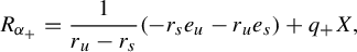 $$ \begin{align} R_{\alpha_+}=\frac{1}{r_u-r_s} (-r_se_u-r_ue_s)+q_+ X, \end{align} $$
and from $\alpha _-(R_{\alpha _+})=0$
, we get
$\alpha _-(R_{\alpha _+})=0$
, we get
 $$ \begin{align} g=-\frac{fr_s}{r_u}. \end{align} $$
Also, using $\alpha _+(R_{\alpha -})=0$
and
$\alpha _+(R_{\alpha -})=0$
and $\alpha _-(R_{\alpha _-})=1$
, we can write (
$\alpha _-(R_{\alpha _-})=1$
, we can write ( $q_-$
being a real function)
$q_-$
being a real function)
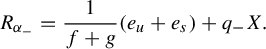 $$ \begin{align} R_{\alpha_-}=\frac{1}{f+g}(e_u+e_s)+q_- X. \end{align} $$
However, we have
 $$ \begin{align} 0=d\alpha_-(R_{\alpha_-},X)&=d\alpha_-(e_s+e_u,X)=-X\cdot\alpha_-(e_s,e_u)-\alpha_-([e_s+e_u,X])\nonumber\\ &\quad\Rightarrow X\cdot f+X\cdot g+gr_s+fr_u=0. \end{align} $$
Using equation 2 in the above, we get
 $$ \begin{align*}X\cdot f+X\cdot g+(f+g)(r_s+r_u)=0,\end{align*} $$
which yields
 $$ \begin{align} r_s+r_u=-X\cdot (f+g).\end{align} $$
Finally, to show that the flow is volume preserving, it suffices to define $\Omega :=e^{f+g}\Omega ^{\alpha _+}$
and use Lemma 4.2 and equation (5) to compute
$\Omega :=e^{f+g}\Omega ^{\alpha _+}$
and use Lemma 4.2 and equation (5) to compute
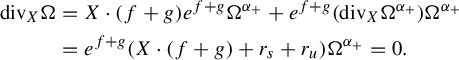 $$ \begin{align*}\mathrm{div}_X\Omega&=X\cdot (f+g)e^{f+g}\Omega^{\alpha_+} + e^{f+g} (\mathrm{div}_X\Omega^{\alpha_+})\Omega^{\alpha_+}\\&=e^{f+g}(X\cdot (f+g)+r_s+r_u)\Omega^{\alpha_+}=0.\\[-3pc]\end{align*} $$
Remark 5.2. It is noteworthy that the above proof shows that in fact, for a volume preserving Anosov flow, we have a function worth of pairs of Reeb vector fields satisfying item (3) of Theorem 5.1. This is useful, in particular, when we require higher regularity of the underlying contact geometry. More precisely, the contact forms in Theorem 5.1(2) are, except in the case of algebraic Anosov flows, only $C^1$
. Therefore, their Reeb vector fields can be only assumed to be
$C^1$
. Therefore, their Reeb vector fields can be only assumed to be $C^0$
in general (this is due to the result of Ghys [Reference Ghys27], which asserts that except in the case of algebraic Anosov flows, the weak stable and unstable bundles cannot be
$C^0$
in general (this is due to the result of Ghys [Reference Ghys27], which asserts that except in the case of algebraic Anosov flows, the weak stable and unstable bundles cannot be $C^2$
). However, if we let go of the symmetry of the contact forms in Theorem 5.1(2), we can achieve higher regularity of the underlying contact geometry in the following sense.
$C^2$
). However, if we let go of the symmetry of the contact forms in Theorem 5.1(2), we can achieve higher regularity of the underlying contact geometry in the following sense.
Let $\phi ^t$
be a volume preserving Anosov flow and
$\phi ^t$
be a volume preserving Anosov flow and $\alpha _+$
a
$\alpha _+$
a $C^\infty $
contact form, which
$C^\infty $
contact form, which $C^1$
-approximates
$C^1$
-approximates $\alpha _u-\alpha _s$
and
$\alpha _u-\alpha _s$
and $\alpha _+(X)=0$
(
$\alpha _+(X)=0$
( $\alpha _u$
and
$\alpha _u$
and $\alpha _s$
are as in the above theorem). Note that
$\alpha _s$
are as in the above theorem). Note that $R_{\alpha _+}$
is
$R_{\alpha _+}$
is $C^\infty $
and
$C^\infty $
and $\xi _-:=\langle R_{\alpha _+},X \rangle $
is a
$\xi _-:=\langle R_{\alpha _+},X \rangle $
is a $C^\infty $
negative contact structure if the
$C^\infty $
negative contact structure if the $C^1$
-approximation of
$C^1$
-approximation of $\alpha _u-\alpha _s$
is small enough. Now, a negative contact form for
$\alpha _u-\alpha _s$
is small enough. Now, a negative contact form for $\xi _-$
is of the form
$\xi _-$
is of the form $\alpha _-:=f\alpha _u+g\alpha _s$
, and to have
$\alpha _-:=f\alpha _u+g\alpha _s$
, and to have $R_{\alpha _-}\subset \xi _+:=\ker {\alpha _+}$
, it suffices to choose any f and g satisfying equation (2), where
$R_{\alpha _-}\subset \xi _+:=\ker {\alpha _+}$
, it suffices to choose any f and g satisfying equation (2), where $r_s$
and
$r_s$
and $r_u$
are the expansion rates associated with
$r_u$
are the expansion rates associated with $\alpha _+$
(as in Remark 4.1). We note that although
$\alpha _+$
(as in Remark 4.1). We note that although $\xi _-$
is
$\xi _-$
is $C^\infty $
, the contact form
$C^\infty $
, the contact form $\alpha _-$
can only be assumed to be
$\alpha _-$
can only be assumed to be $C^1$
in general.
$C^1$
in general.
Corollary of the Proof 5.3
In Theorem 5.1(3), the supporting bi-contact structure $(\xi _-,\xi _+)$
, as well as at least one of
$(\xi _-,\xi _+)$
, as well as at least one of $R_{\alpha _+}$
or
$R_{\alpha _+}$
or $R_{\alpha _-}$
, can be chosen to be
$R_{\alpha _-}$
, can be chosen to be $C^\infty $
.
$C^\infty $
.
Theorem 5.1 gives examples of $(-1)$
-Cartan structures and taut contact hyperbolas whenever we have volume preserving flows, including the case of algebraic Anosov flows, and more interestingly, we get new examples on hyperbolic manifolds using the examples of contact Anosov flows on those manifolds [Reference Foulon and Hasselblatt21]. The construction also yields new examples of
$(-1)$
-Cartan structures and taut contact hyperbolas whenever we have volume preserving flows, including the case of algebraic Anosov flows, and more interestingly, we get new examples on hyperbolic manifolds using the examples of contact Anosov flows on those manifolds [Reference Foulon and Hasselblatt21]. The construction also yields new examples of $(-1)$
-Cartan structures on any manifold supporting a transitive Anosov flow, many of which are not contact [Reference Asaoka5, Reference Béguin, Bonatti and Yu10].
$(-1)$
-Cartan structures on any manifold supporting a transitive Anosov flow, many of which are not contact [Reference Asaoka5, Reference Béguin, Bonatti and Yu10].
Corollary 5.4. There exist infinitely many hyperbolic manifolds which admit a $(-1)$
-Cartan structure (and, in particular, a taut contact hyperbola).
$(-1)$
-Cartan structure (and, in particular, a taut contact hyperbola).
5.2 From the viewpoint of Liouville geometry
In [Reference Hozoori33], we have shown how from an Anosov flow X on a 3-manifold M, we can construct two Liouville pairs, $(\alpha _-,\alpha _+)$
and
$(\alpha _-,\alpha _+)$
and $(-\alpha _-,\alpha _+)$
, where
$(-\alpha _-,\alpha _+)$
, where $(\xi _-:=\ker {\alpha _-},\xi _+:=\ker {\alpha _+})$
is a supporting bi-contact structure for X. That is,
$(\xi _-:=\ker {\alpha _-},\xi _+:=\ker {\alpha _+})$
is a supporting bi-contact structure for X. That is, $\omega _1:=d\alpha _1$
and
$\omega _1:=d\alpha _1$
and $\omega _2:=d\alpha _2$
are exact symplectic structures on
$\omega _2:=d\alpha _2$
are exact symplectic structures on $[-1,1]_t\times M$
, where
$[-1,1]_t\times M$
, where $\alpha _1:=(1-t)\alpha _-+(1+t)\alpha _+$
and
$\alpha _1:=(1-t)\alpha _-+(1+t)\alpha _+$
and $\alpha _2:=(1-t)\alpha _--(1+t)\alpha _+$
.
$\alpha _2:=(1-t)\alpha _--(1+t)\alpha _+$
.
Recall that $(W,d\alpha )$
is an exact symplectic 4-manifold if W is an oriented 4-manifold (with boundary) and
$(W,d\alpha )$
is an exact symplectic 4-manifold if W is an oriented 4-manifold (with boundary) and $d\alpha $
is an exact symplectic structure on W, that is,
$d\alpha $
is an exact symplectic structure on W, that is, $d\alpha \wedge d\alpha>0$
. For any exact symplectic manifold
$d\alpha \wedge d\alpha>0$
. For any exact symplectic manifold $(W,d\alpha )$
, there exists a unique vector field Y, such that
$(W,d\alpha )$
, there exists a unique vector field Y, such that $\iota _Y d\alpha =\alpha $
, or equivalently
$\iota _Y d\alpha =\alpha $
, or equivalently $\mathcal {L}_Y d\alpha =d\alpha $
. Such a vector field is called a Liouville vector field if it points in the outward direction on
$\mathcal {L}_Y d\alpha =d\alpha $
. Such a vector field is called a Liouville vector field if it points in the outward direction on $\partial W$
, and the pair
$\partial W$
, and the pair $(W,Y)$
is called a Liouville structure. We note that this is the case for an exact symplectic manifold constructed from Anosov 3-flows above, since it is a symplectic filling for the contact manifold
$(W,Y)$
is called a Liouville structure. We note that this is the case for an exact symplectic manifold constructed from Anosov 3-flows above, since it is a symplectic filling for the contact manifold $(M,\xi _+)\cup (-M,\xi _-)$
.
$(M,\xi _+)\cup (-M,\xi _-)$
.
The relation between the associated Liouville vector field and the underlying Anosov vector field is more subtle in the general case of $C^1$
Anosov flows. However, for
$C^1$
Anosov flows. However, for $C^{1+}$
volume preserving Anosov flows, such a connection becomes very straightforward thanks to the symmetries implied by the existence of an invariant volume form and the fact that in this case, the weak stable and unstable bundles are
$C^{1+}$
volume preserving Anosov flows, such a connection becomes very straightforward thanks to the symmetries implied by the existence of an invariant volume form and the fact that in this case, the weak stable and unstable bundles are $C^1$
[Reference Hasselblatt30, Reference Hurder and Katok35].
$C^1$
[Reference Hasselblatt30, Reference Hurder and Katok35].
In what follows, we let $(\alpha _-=\alpha _u+\alpha _s,\alpha _+=\alpha _u-\alpha _s)$
be the
$(\alpha _-=\alpha _u+\alpha _s,\alpha _+=\alpha _u-\alpha _s)$
be the $(-1)$
-Cartan structure of Theorem 5.1 (in particular,
$(-1)$
-Cartan structure of Theorem 5.1 (in particular, $\Omega ^{\alpha _+}=\alpha _s\wedge \alpha _u\wedge \alpha _X$
is a positive volume form for any 1-form
$\Omega ^{\alpha _+}=\alpha _s\wedge \alpha _u\wedge \alpha _X$
is a positive volume form for any 1-form $\alpha _X$
with
$\alpha _X$
with $\alpha _X(X)=1$
). We have the 1-form
$\alpha _X(X)=1$
). We have the 1-form $\alpha _1=(1-t)\alpha _-+(1+t)\alpha _+=2\alpha _u-2t\alpha _s$
on
$\alpha _1=(1-t)\alpha _-+(1+t)\alpha _+=2\alpha _u-2t\alpha _s$
on $ [-1,1]_t\times M$
, and compute
$ [-1,1]_t\times M$
, and compute
 $$ \begin{align*}d\alpha_1\wedge d\alpha_1&=\{ 2d\alpha_u-2dt\wedge \alpha_s-2td\alpha_s \} \wedge \{ 2d\alpha_u-2dt\wedge \alpha_s-2td\alpha_s \}\\&=-4dt\wedge \alpha_s\wedge d\alpha_u=4r_udt\wedge \Omega^{\alpha_+},\end{align*} $$
implying that $( [-1,1]_t\times M,d\alpha _1)$
is an exact symplectic manifold. Similarly, we can show
$( [-1,1]_t\times M,d\alpha _1)$
is an exact symplectic manifold. Similarly, we can show $d\alpha _2\wedge d\alpha _2=-4r_sdt\wedge \Omega ^{\alpha _-}$
, yielding another exact symplectic structure on
$d\alpha _2\wedge d\alpha _2=-4r_sdt\wedge \Omega ^{\alpha _-}$
, yielding another exact symplectic structure on $[-1,1]_t\times M$
. Notice that with the above assumptions, we have
$[-1,1]_t\times M$
. Notice that with the above assumptions, we have $r_u=-r_s>0$
and
$r_u=-r_s>0$
and $\Omega ^{\alpha _+}=\Omega ^{\alpha _-}$
. However, the fact that the weak stable and unstable bundles are
$\Omega ^{\alpha _+}=\Omega ^{\alpha _-}$
. However, the fact that the weak stable and unstable bundles are $C^1$
in this case, thanks to the Hölder continuity of the derivatives of the flow, plays a crucial role in preserving the symmetry when going from a metric description of the underlying Anosov flow to a contact geometric one, and hence, significantly simplifying the construction of the above Liouville pairs, compared to Anosov flows of lower regularity studied in [Reference Hozoori33]. We also remark that unless X is an algebraic Anosov flow [Reference Ghys27], the
$C^1$
in this case, thanks to the Hölder continuity of the derivatives of the flow, plays a crucial role in preserving the symmetry when going from a metric description of the underlying Anosov flow to a contact geometric one, and hence, significantly simplifying the construction of the above Liouville pairs, compared to Anosov flows of lower regularity studied in [Reference Hozoori33]. We also remark that unless X is an algebraic Anosov flow [Reference Ghys27], the $(-1)$
-Cartan structure is a priori only
$(-1)$
-Cartan structure is a priori only $C^1$
, and therefore, the 2-forms
$C^1$
, and therefore, the 2-forms $d\alpha _1$
and
$d\alpha _1$
and $d\alpha _2$
above are exact symplectic structures, only in the
$d\alpha _2$
above are exact symplectic structures, only in the $C^0$
sense.
$C^0$
sense.
Now, if we define the vector field $Y_1:=({1}/{r_u})X+2t\partial _t$
, we can compute
$Y_1:=({1}/{r_u})X+2t\partial _t$
, we can compute
 $$ \begin{align*}\iota_{Y_1} d\alpha_1=\frac{2}{r_u} \iota_X d\alpha_u -4t\alpha_s-\frac{2t}{r_u} \iota_Xd\alpha_s=2\alpha_u-4t\alpha_s+2t\alpha_s=\alpha_1.\end{align*} $$
Therefore, $Y_1$
is the Liouville vector field for
$Y_1$
is the Liouville vector field for $([-1,1]_t\times M,d\alpha _1)$
. Notice that a similar computation helps us compute the Liouville vector field of
$([-1,1]_t\times M,d\alpha _1)$
. Notice that a similar computation helps us compute the Liouville vector field of $([-1,1]_t\times M,d\alpha _2)$
. It can be seen [Reference Simić48] that the 1-forms
$([-1,1]_t\times M,d\alpha _2)$
. It can be seen [Reference Simić48] that the 1-forms $\alpha _u$
and
$\alpha _u$
and $\alpha _s$
can be chosen such that
$\alpha _s$
can be chosen such that $r_u$
and
$r_u$
and $r_s$
are
$r_s$
are $C^1$
. In that case, it is noteworthy and surprising that although the constructed symplectic structures above are a priori only
$C^1$
. In that case, it is noteworthy and surprising that although the constructed symplectic structures above are a priori only $C^0$
, their corresponding Liouville vector fields are
$C^0$
, their corresponding Liouville vector fields are $C^1$
.
$C^1$
.
Now, we can consider the vector field $X_L:=({1}/{r_u})X$
, which generates a reparameterization of the original flow. Its associated expansion rates are
$X_L:=({1}/{r_u})X$
, which generates a reparameterization of the original flow. Its associated expansion rates are $r^{\prime }_u={r_u}/{r_u}=1$
and
$r^{\prime }_u={r_u}/{r_u}=1$
and $r^{\prime }_s={r_s}/ {r_u}=-1$
(see Remark 3.18 of [Reference Hozoori33]) and we have
$r^{\prime }_s={r_s}/ {r_u}=-1$
(see Remark 3.18 of [Reference Hozoori33]) and we have $Y_1|_{\{ 0\}\times M}=X_L$
. We call such
$Y_1|_{\{ 0\}\times M}=X_L$
. We call such $X_L$
the Liouville reparameterization of a volume preserving Anosov 3-flow (in the sense of [Reference Simić48], this is the synchronization of the flow with respect to both stable and unstable directions, simultaneously).
$X_L$
the Liouville reparameterization of a volume preserving Anosov 3-flow (in the sense of [Reference Simić48], this is the synchronization of the flow with respect to both stable and unstable directions, simultaneously).
The following theorem proves that the Liouville reparameterization of a volume preserving Anosov flow has even a closer relation to the underlying Reeb dynamics of Theorem 5.1.
Theorem 5.5. Let X be the generating vector field of a volume preserving Anosov flow. If $X_L$
is the generating vector field for the Liouville reparameterization of the flow, the following hold:
$X_L$
is the generating vector field for the Liouville reparameterization of the flow, the following hold:
-
(1) the flow generated by
$X_L$
preserves the transverse plane field
$\langle R_{\alpha _-},R_{\alpha _+} \rangle $
, where
$R_{\alpha _-}$
and
$R_{\alpha _+}$
are the Reeb vector fields of Theorem 1.6(2); -
(2) the pair
$(M,X_L)$
can be extended to a Liouville structure
$([-1,1]\times M,Y)$
, such that
$([-1,1]\times M,Y)|_{\{ 0\} \times M}=(M,X_L).$


Proof. The above argument yields item (2). To prove item (1), let ( $\alpha _-=\alpha _u+\alpha _s,\alpha _+=\alpha _u-\alpha _s$
) be the
$\alpha _-=\alpha _u+\alpha _s,\alpha _+=\alpha _u-\alpha _s$
) be the $(-1)$
-Cartan structure of part (2) in Theorem 5.1. We have
$(-1)$
-Cartan structure of part (2) in Theorem 5.1. We have
 $$ \begin{align*}\mathcal{L}_{X_L}\alpha_+=\mathcal{L}_{X_L}(\alpha_u-\alpha_s)=\alpha_u+\alpha_s=\alpha_-.\end{align*} $$
Similarly, one can show $\mathcal {L}_{X_L}\alpha _-=\alpha _+$
. Define the 1-form
$\mathcal {L}_{X_L}\alpha _-=\alpha _+$
. Define the 1-form $\alpha _{X_L}$
by letting
$\alpha _{X_L}$
by letting $\alpha _{X_L}(X_L)=1$
and
$\alpha _{X_L}(X_L)=1$
and $\alpha _{X_L}(\langle R_{\alpha _-},R_{\alpha _+}\rangle )=0$
. The goal is to prove
$\alpha _{X_L}(\langle R_{\alpha _-},R_{\alpha _+}\rangle )=0$
. The goal is to prove $\mathcal {L}_{X_L}\alpha _{X_L}=0$
. Note that by construction,
$\mathcal {L}_{X_L}\alpha _{X_L}=0$
. Note that by construction, $\alpha _{X_L}$
is differentiable along the flow and
$\alpha _{X_L}$
is differentiable along the flow and $(\mathcal {L}_{X_L}\alpha _{X_L})\wedge \alpha _{X_L}=0$
.
$(\mathcal {L}_{X_L}\alpha _{X_L})\wedge \alpha _{X_L}=0$
.
Also, by plugging the basis $(R_{\alpha _-},R_{\alpha _+},X_L)$
, we can observe
$(R_{\alpha _-},R_{\alpha _+},X_L)$
, we can observe
 $$ \begin{align*}d\alpha_+=\alpha_{X_L} \wedge \alpha_- \quad\text{and}\quad d\alpha_-=\alpha_{X_L}\wedge \alpha_+,\end{align*} $$
which implies
 $$ \begin{align*}(\mathcal{L}_{X_L}\alpha_{X_L})\wedge \alpha_-&=\mathcal{L}_{X_L}(\alpha_{X_L}\wedge \alpha_-)-\alpha_{X_L}\wedge \mathcal{L}_{X_L}\alpha_-\\&=\mathcal{L}_{X_L} d\alpha_+-\alpha_{X_L}\wedge\alpha_+=d(\mathcal{L}_{X_L} \alpha_+)-\alpha_{X_L}\wedge\alpha_+=d\alpha_--d\alpha_-=0.\end{align*} $$
Similarly, we have $(\mathcal {L}_{X_L}\alpha _{X_L})\wedge \alpha _+=0$
. This yields
$(\mathcal {L}_{X_L}\alpha _{X_L})\wedge \alpha _+=0$
. This yields $\mathcal {L}_{X_L}\alpha _{X_L}=0$
, completing the proof.
$\mathcal {L}_{X_L}\alpha _{X_L}=0$
, completing the proof.
6 Applications to bi-contact surgeries
In this section, we discuss the implications of our work in the surgery theory of Anosov flows. Theorem 5.1 shows that for volume preserving Anosov flows, the Reeb vector fields associated with the supporting bi-contact structure $(\xi _-=\ker {\alpha _-},\xi _+=\ker {\alpha _+})$
can be contained in one another. In this case, if we push a periodic orbit of the flow
$(\xi _-=\ker {\alpha _-},\xi _+=\ker {\alpha _+})$
can be contained in one another. In this case, if we push a periodic orbit of the flow $\gamma _0$
, which is a Legendrian knot for both
$\gamma _0$
, which is a Legendrian knot for both $\xi _-$
and
$\xi _-$
and $\xi _+$
, along one of these Reeb vector fields, say
$\xi _+$
, along one of these Reeb vector fields, say $R_{\alpha _+}$
, it stays Legendrian for
$R_{\alpha _+}$
, it stays Legendrian for $\xi _+$
(since
$\xi _+$
(since $R_{\alpha _+}$
preserves
$R_{\alpha _+}$
preserves $\xi _+$
) and it immediately becomes transverse to
$\xi _+$
) and it immediately becomes transverse to $\xi _-$
(since
$\xi _-$
(since $R_{\alpha _+}$
is a Legendrian vector field for
$R_{\alpha _+}$
is a Legendrian vector field for $\xi _-$
). We call such a knot a Legendrian-transverse knot.
$\xi _-$
). We call such a knot a Legendrian-transverse knot.
In [Reference Salmoiraghi45, Reference Salmoiraghi46], Salmoiraghi develops two flavors of bi-contact surgery operations in a neighborhood of a Legendrian-transverse knot. One of these operations is applied by cutting the manifold on an annulus, which is tangent to the flow and contains the Legendrian-transverse knot, and then glueing back using a Dehn twist [Reference Salmoiraghi45]. The other operation is applied to a transverse annulus containing such a knot [Reference Salmoiraghi46]. Moreover, he shows that using the coordinates coming from the above argument on the Reeb vector field, one can reconstruct the classical Goodman surgery in the neighborhood of a periodic orbit of an Anosov flow using the bi-contact surgery of [Reference Salmoiraghi46]. However, notice that in the above argument, it suffices for the Reeb vector field of just one of the contact structures to be contained in the other contact structure only in a small neighborhood of the periodic orbit on which one wants to apply the Goodman surgery. In the following, we show that this is possible for any (possibly non volume preserving) Anosov flow. The main idea is to show that one can assume that the flow has constant divergence along a fixed periodic orbit.
Theorem 6.1. Let $\phi ^t$
be an Anosov flow. Given any periodic orbit
$\phi ^t$
be an Anosov flow. Given any periodic orbit $\gamma _0$
, there exists a supporting bi-contact structure
$\gamma _0$
, there exists a supporting bi-contact structure $(\xi _-,\xi _+=\ker {\alpha _+})$
such that we have
$(\xi _-,\xi _+=\ker {\alpha _+})$
such that we have $R_{\alpha _+}\subset \xi _-$
in a regular neighborhood of
$R_{\alpha _+}\subset \xi _-$
in a regular neighborhood of $\gamma _0$
. Therefore, there exists an isotopy
$\gamma _0$
. Therefore, there exists an isotopy $\{\gamma _t\}_{t\in [0,1]}$
, which is supported in an arbitrary small neighborhood of
$\{\gamma _t\}_{t\in [0,1]}$
, which is supported in an arbitrary small neighborhood of $\gamma _0$
, and
$\gamma _0$
, and $\gamma _t$
is a Legendrian-transverse knot for any
$\gamma _t$
is a Legendrian-transverse knot for any $0<t\leq 1$
.
$0<t\leq 1$
.
Proof. As discussed above, it is enough to show that there exists a tubular neighborhood $N(\gamma _0)$
and a pair of contact forms
$N(\gamma _0)$
and a pair of contact forms $\alpha _+$
and
$\alpha _+$
and $\alpha _-$
such that
$\alpha _-$
such that $(\ker {\alpha _-},\ker {\alpha _+})$
is a supporting bi-contact structure for X and
$(\ker {\alpha _-},\ker {\alpha _+})$
is a supporting bi-contact structure for X and $\alpha _-(R_{\alpha _+})=0$
. It is easy to show that this would have been possible if the associated expansion rates were constant. The idea of the proof is to find an appropriate norm which satisfies this condition on
$\alpha _-(R_{\alpha _+})=0$
. It is easy to show that this would have been possible if the associated expansion rates were constant. The idea of the proof is to find an appropriate norm which satisfies this condition on $\gamma _0$
and use the openness of the contact condition. To do so, we need an approximation technique similar to the one used in the main theorem of [Reference Hozoori33]. The only caveat is that we need our approximation not to affect the preassigned norm on
$\gamma _0$
and use the openness of the contact condition. To do so, we need an approximation technique similar to the one used in the main theorem of [Reference Hozoori33]. The only caveat is that we need our approximation not to affect the preassigned norm on $\gamma _0$
.
$\gamma _0$
.
Let T be the period of $\gamma _0$
, and
$\gamma _0$
, and $\unicode{x3bb} ^{\gamma _0}_u$
and
$\unicode{x3bb} ^{\gamma _0}_u$
and $\unicode{x3bb} ^{\gamma _0}_s$
be the eigenvalues of the return map along
$\unicode{x3bb} ^{\gamma _0}_s$
be the eigenvalues of the return map along $\gamma _0$
corresponding to the unstable and stable directions, respectively. We can choose a X-differentiable norm on
$\gamma _0$
corresponding to the unstable and stable directions, respectively. We can choose a X-differentiable norm on $TM/\langle X \rangle |_{\gamma _0}$
such that the induced expansion rates
$TM/\langle X \rangle |_{\gamma _0}$
such that the induced expansion rates $r_u|_{\gamma _0}$
and
$r_u|_{\gamma _0}$
and $r_s|_{\gamma _0}$
are constants satisfying
$r_s|_{\gamma _0}$
are constants satisfying $e^{r_uT}=\unicode{x3bb} ^{\gamma _0}_u$
and
$e^{r_uT}=\unicode{x3bb} ^{\gamma _0}_u$
and $e^{r_sT}=\unicode{x3bb} ^{\gamma _0}_s$
. We can then extend such a norm to some X-differentiable norm on
$e^{r_sT}=\unicode{x3bb} ^{\gamma _0}_s$
. We can then extend such a norm to some X-differentiable norm on $TM/\langle X\rangle \simeq E^s\oplus E^u$
in a neighborhood of
$TM/\langle X\rangle \simeq E^s\oplus E^u$
in a neighborhood of $\gamma _0$
. Let
$\gamma _0$
. Let $N(\gamma _0)$
be a possibly smaller neighborhood, on which
$N(\gamma _0)$
be a possibly smaller neighborhood, on which $r_s<0<r_u$
.
$r_s<0<r_u$
.
We define the 1-forms $\tilde {\alpha }_u$
and
$\tilde {\alpha }_u$
and $\tilde {\alpha }_u$
by letting
$\tilde {\alpha }_u$
by letting $\tilde {\alpha }_u(E^s)=\tilde {\alpha }_s(E^u)=0$
and
$\tilde {\alpha }_u(E^s)=\tilde {\alpha }_s(E^u)=0$
and $\tilde {\alpha }_u(e_u)=\tilde {\alpha }_s(e_s)=1$
, where
$\tilde {\alpha }_u(e_u)=\tilde {\alpha }_s(e_s)=1$
, where $e_s \in E^s$
and
$e_s \in E^s$
and $e_u \in E^u$
are the unit vectors with respect to our norm. We can
$e_u \in E^u$
are the unit vectors with respect to our norm. We can $C^0$
-approximate
$C^0$
-approximate $\tilde {\alpha }_u$
and
$\tilde {\alpha }_u$
and $\tilde {\alpha }_u$
by
$\tilde {\alpha }_u$
by $C^\infty $
1-forms
$C^\infty $
1-forms $\bar {\alpha }_u$
and
$\bar {\alpha }_u$
and $\bar {\alpha }_u$
, and find X-differentiable functions
$\bar {\alpha }_u$
, and find X-differentiable functions $f_u$
and
$f_u$
and $f_s$
such that
$f_s$
such that $f_u\bar {\alpha }_u(e_u)=f_s\bar {\alpha }_s(e_s)=1$
. Using the following lemma, we can approximate these functions with appropriate
$f_u\bar {\alpha }_u(e_u)=f_s\bar {\alpha }_s(e_s)=1$
. Using the following lemma, we can approximate these functions with appropriate $C^1$
functions to serve our goal.
$C^1$
functions to serve our goal.
Lemma 6.2. If f is X-differentiable and $\eta $
-Hölder continuous and
$\eta $
-Hölder continuous and $\gamma $
is a periodic orbit of X (a
$\gamma $
is a periodic orbit of X (a $C^1$
flow on n-dimensional closed manifold M), then for any
$C^1$
flow on n-dimensional closed manifold M), then for any $\epsilon>0$
, there exists a
$\epsilon>0$
, there exists a $C^1$
function
$C^1$
function $\bar {f}$
such that
$\bar {f}$
such that $f|_{\gamma }=\bar {f}|_{\gamma }$
, and we have
$f|_{\gamma }=\bar {f}|_{\gamma }$
, and we have $|f-\bar {f}|<\epsilon $
and
$|f-\bar {f}|<\epsilon $
and $|X\cdot f-X\cdot \bar {f}|<\epsilon $
.
$|X\cdot f-X\cdot \bar {f}|<\epsilon $
.
Proof. Let $N_\delta (\gamma )$
be a sufficiently small tubular neighborhood of
$N_\delta (\gamma )$
be a sufficiently small tubular neighborhood of $\gamma $
, on which the function
$\gamma $
, on which the function $d(x)$
, measuring the distance of
$d(x)$
, measuring the distance of $x\in M$
from
$x\in M$
from $\gamma $
, is
$\gamma $
, is $C^1$
, that is,
$C^1$
, that is, $N_\delta =\{x\in M | d(x)<\delta \}$
. Let
$N_\delta =\{x\in M | d(x)<\delta \}$
. Let $\bar {d}(x)$
be any
$\bar {d}(x)$
be any $C^1$
function on M, where
$C^1$
function on M, where $\bar {d}(x)=d(x)$
on
$\bar {d}(x)=d(x)$
on $N_{{\delta }/{2}}(\gamma ) \subset N_\delta (\gamma )$
and
$N_{{\delta }/{2}}(\gamma ) \subset N_\delta (\gamma )$
and $\bar {d}(x)\neq 0$
everywhere.
$\bar {d}(x)\neq 0$
everywhere.
Now, we can write $f(x)=f^\gamma (x)+\bar {d}^{{\eta }/{2}}(x)g(x)$
, where
$f(x)=f^\gamma (x)+\bar {d}^{{\eta }/{2}}(x)g(x)$
, where $f^\gamma (x)$
is any
$f^\gamma (x)$
is any $C^1$
extension of
$C^1$
extension of $f|_{\gamma }$
on M and
$f|_{\gamma }$
on M and $g(x)$
is a well-defined, continuous and X-differentiable function on
$g(x)$
is a well-defined, continuous and X-differentiable function on $M\backslash \gamma $
. We extend g to M by letting
$M\backslash \gamma $
. We extend g to M by letting $g(\gamma )=0$
.
$g(\gamma )=0$
.
Claim 6.3. The function g is continuous and X-differentiable on $N_\delta (\gamma )$
.
$N_\delta (\gamma )$
.
Proof. Notice
 $$ \begin{align*}\lim_{d(x)\rightarrow 0}g(x)=\lim_{d(x)\rightarrow 0}\frac{f(x)-f^\gamma(x)}{d^{{\eta}/{2}}(x)}=\lim_{d(x)\rightarrow 0}\frac{f(x)-f^\gamma(x)}{d^\eta(x)} d^{{\eta}/{2}}(x)=0.\end{align*} $$
The last equality follows from f being $\eta $
-Hölder continuous. Therefore, g is a continuous function on
$\eta $
-Hölder continuous. Therefore, g is a continuous function on $N_\delta (\gamma )$
(in fact, it is
$N_\delta (\gamma )$
(in fact, it is ${\eta }/{2}$
-Hölder continuous). Moreover, g is X-differentiable in this neighborhood, since we have
${\eta }/{2}$
-Hölder continuous). Moreover, g is X-differentiable in this neighborhood, since we have $X\cdot g|_\gamma =0$
.
$X\cdot g|_\gamma =0$
.
Now, we use Lemma 4.2 of [Reference Hozoori33] to find a $C^1$
function
$C^1$
function $\bar {g}$
, where
$\bar {g}$
, where $|g-\bar {g}|$
and
$|g-\bar {g}|$
and $|X\cdot g-X\cdot \bar {g}|$
are arbitrary small. In fact, if we define
$|X\cdot g-X\cdot \bar {g}|$
are arbitrary small. In fact, if we define $\bar {f}:=f^{\gamma _0}+\bar {d}^{{\eta }/{2}}\bar {g}$
, we can find an approximation of g such that
$\bar {f}:=f^{\gamma _0}+\bar {d}^{{\eta }/{2}}\bar {g}$
, we can find an approximation of g such that $\bar {f}$
is the desired
$\bar {f}$
is the desired $C^1$
function. This completes the proof of Lemma 6.2.
$C^1$
function. This completes the proof of Lemma 6.2.
Let $\bar {f}_s$
and
$\bar {f}_s$
and $\bar {f}_u$
be the approximations of
$\bar {f}_u$
be the approximations of $f_s$
and
$f_s$
and $f_u$
as in Lemma 6.2. As in [Reference Hozoori33], we can define the
$f_u$
as in Lemma 6.2. As in [Reference Hozoori33], we can define the $C^1$
contact forms
$C^1$
contact forms $\alpha _+$
with
$\alpha _+$
with $e^{\prime }_s\in E^s\subset TM$
,
$e^{\prime }_s\in E^s\subset TM$
, $e^{\prime }_u \in E^u \subset TM$
,
$e^{\prime }_u \in E^u \subset TM$
, $r^{\prime }_u$
, and
$r^{\prime }_u$
, and $r^{\prime }_s$
induced by
$r^{\prime }_s$
induced by $\alpha _+$
, as in Remark 4.1, such that when restricted to
$\alpha _+$
, as in Remark 4.1, such that when restricted to $\gamma _0$
, we have
$\gamma _0$
, we have $\alpha _+(e_u)=\bar {f}_u\bar {\alpha }_u(e_u)=f_u\bar {\alpha }_u(e_u)=1$
and similarly
$\alpha _+(e_u)=\bar {f}_u\bar {\alpha }_u(e_u)=f_u\bar {\alpha }_u(e_u)=1$
and similarly $\alpha _+(e_s)=1$
, which yields
$\alpha _+(e_s)=1$
, which yields $e_s=e^{\prime }_s$
,
$e_s=e^{\prime }_s$
, $e_u=e^{\prime }_u$
,
$e_u=e^{\prime }_u$
, $r_s=r^{\prime }_s$
, and
$r_s=r^{\prime }_s$
, and $r_u=r^{\prime }_u$
(we refer the reader to [Reference Hozoori33] for the the technical details of the approximations used in the definition. It is enough for us to know that the induced unit vectors and expansion rates from these approximating contact forms are arbitrary close to the ones we started with, while agreeing on
$r_u=r^{\prime }_u$
(we refer the reader to [Reference Hozoori33] for the the technical details of the approximations used in the definition. It is enough for us to know that the induced unit vectors and expansion rates from these approximating contact forms are arbitrary close to the ones we started with, while agreeing on $\gamma _0$
). As in equation (1), we have
$\gamma _0$
). As in equation (1), we have $R_{\alpha ^{\prime }_+}={1}/({r^{\prime }_u-r^{\prime }_s})\{-r^{\prime }_ue^{\prime }_s-r^{\prime }_se^{\prime }_u\}+q_+ X$
for some real function
$R_{\alpha ^{\prime }_+}={1}/({r^{\prime }_u-r^{\prime }_s})\{-r^{\prime }_ue^{\prime }_s-r^{\prime }_se^{\prime }_u\}+q_+ X$
for some real function $q_+$
. Let
$q_+$
. Let $\xi ^{\prime }_-:=\langle R_{\alpha _+},X\rangle $
.
$\xi ^{\prime }_-:=\langle R_{\alpha _+},X\rangle $
.
Claim 6.4. There exists a regular neighborhood $N(\gamma _0)$
on which
$N(\gamma _0)$
on which $\xi ^{\prime }_-$
is a negative contact structure.
$\xi ^{\prime }_-$
is a negative contact structure.
Proof. Choose a 1-form $\alpha _-$
such that
$\alpha _-$
such that $\xi ^{\prime }_-:=\ker {\alpha _-}$
and
$\xi ^{\prime }_-:=\ker {\alpha _-}$
and $\alpha _-(e^{\prime }_s+e^{\prime }_u)>0$
. Compute
$\alpha _-(e^{\prime }_s+e^{\prime }_u)>0$
. Compute
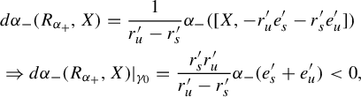 $$ \begin{align*}&d\alpha_-(R_{\alpha_+},X)=\frac{1}{r^{\prime}_u-r^{\prime}_s}\alpha_-([X,-r^{\prime}_ue^{\prime}_s-r^{\prime}_se^{\prime}_u])\\&\Rightarrow d\alpha_-(R_{\alpha_+},X)|_{\gamma_0}=\frac{r^{\prime}_sr^{\prime}_u}{r^{\prime}_u-r^{\prime}_s}\alpha_-(e^{\prime}_s+e^{\prime}_u)<0,\end{align*} $$
where in the last equality, we have used the fact that, by construction, we have $X\cdot r^{\prime }_s=X\cdot r_s=X\cdot r^{\prime }_u=X\cdot r_u=0$
on
$X\cdot r^{\prime }_s=X\cdot r_s=X\cdot r^{\prime }_u=X\cdot r_u=0$
on $\gamma _0$
. Thanks to the openness of the contact condition,
$\gamma _0$
. Thanks to the openness of the contact condition, $\xi ^{\prime }_-$
is a negative contact structure in some tubular neighborhood
$\xi ^{\prime }_-$
is a negative contact structure in some tubular neighborhood $N(\gamma _0)$
.
$N(\gamma _0)$
.
We can extend $\xi '|_{N(\gamma _0)}$
to some negative contact structure
$\xi '|_{N(\gamma _0)}$
to some negative contact structure $\xi _-$
on M such that the supporting bi-contact structure
$\xi _-$
on M such that the supporting bi-contact structure $(\xi _-,\xi _+=\ker {\alpha _+})$
has the desired properties.
$(\xi _-,\xi _+=\ker {\alpha _+})$
has the desired properties.
Corollary 6.5. The bi-contact surgeries of Salmoiraghi [Reference Salmoiraghi45, Reference Salmoiraghi46] can be applied in an arbitrary small neighborhood of a periodic orbit of any Anosov flow. In particular, the bi-contact surgery of [Reference Salmoiraghi46] reconstructs the Goodman surgery.
Acknowledgements
I want to thank my advisor, John Etnyre, for constant support and encouragement. I am also very grateful to Meysam Nassiri, Federico Salmoiraghi, Domenico Perrone, Thomas Barthelmé, Masayuki Asaoka, and Steven Hurder for helpful conversations. Finally, I owe a debt of gratitude to the reviewers for thoughtful examination and insightful suggestions. The author was partially funded by an NSF grant DMS-1906414.


 Open access