


1. Introduction
Turbulent convection, one of the most complicated fluid motions, is ubiquitous in nature and industrial processes. As two essential elements of fluid dynamics, buoyancy and shear play important roles in many kinds of turbulent flows. Under gravity or other body force fields, buoyancy is generated by the inhomogeneous density distribution of fluid. When the buoyancy force is large, it can induce instability and drive the convection. Rayleigh–Bénard (RB) convection is one typical paradigm of buoyancy-driven convection and has been studied extensively in scientific research (Ahlers, Grossmann & Lohse Reference Ahlers, Grossmann and Lohse2009; Lohse & Xia Reference Lohse and Xia2010; Chillà & Schumacher Reference Chillà and Schumacher2012; Xia Reference Xia2013). In the RB cell, the fluid is heated from below and cooled from above under gravity. Due to the thermal expansion of the fluid, buoyancy appears and drives the convection. Some manifold and involute flow structures are formed in the cell (Niemela et al. Reference Niemela, Skrbek, Sreenivasan and Donnelly2001; Xi, Lam & Xia Reference Xi, Lam and Xia2004; Sun, Xia & Tong Reference Sun, Xia and Tong2005; Wang et al. Reference Wang, Jiang, Jiang, Sun and Liu2021). Moreover, apart from the classical RB model with rectangular cells, annular (Pitz, Marxen & Chew Reference Pitz, Marxen and Chew2017; Kang et al. Reference Kang, Meyer, Yoshikawa and Mutabazi2019; Jiang et al. Reference Jiang, Zhu, Wang, Huisman and Sun2020; Rouhi et al. Reference Rouhi, Lohse, Marusic, Sun and Chung2021; Wang et al. Reference Wang, Liu, Zhou and Sun2023) and spherical (Gastine, Wicht & Aurnou Reference Gastine, Wicht and Aurnou2015) RB cells also attract a lot of interest. The uniform gravity is substituted by the centrifugal force or gravity that varies in the direction of the temperature gradient. Different from buoyancy, shear contributes to the flow mainly by the motion of the system boundary. Taylor–Couette (TC) flow, the flow impelled by two concentric cylinders rotating independently, is a widely used canonical model to study the effect of shear. Secondary flows are caused by the centrifugal instability, and then many complicated flow structures, including turbulent Taylor vortex flow and wavelets, are generated at high Reynolds numbers (Bayly Reference Bayly1988; Esser & Grossmann Reference Esser and Grossmann1996; Brauckmann & Eckhardt Reference Brauckmann and Eckhardt2013; Ostilla-Mónico et al. Reference Ostilla-Mónico, Huisman, Jannink, Van Gils, Verzicco, Grossmann, Sun and Lohse2014a; Grossmann, Lohse & Sun Reference Grossmann, Lohse and Sun2016).
Transport efficiency is an important quantity in both RB convection and TC flow, as the physical quantities being transferred are temperature and angular velocity, respectively (Eckhardt, Grossmann & Lohse Reference Eckhardt, Grossmann and Lohse2007). In non-dimensional forms, there exist scaling laws in RB convection, between the dimensionless heat flux (measured by the Nusselt number  $Nu_h$) and the dimensionless buoyancy-driven strength (measured by the Rayleigh number $Ra$) (Castaing et al. Reference Castaing, Gunaratne, Heslot, Kadanoff, Libchaber, Thomae, Wu, Zaleski and Zanetti1989; Shraiman & Siggia Reference Shraiman and Siggia1990; Grossmann & Lohse Reference Grossmann and Lohse2000); similar scaling laws occur in TC flow as well, between the dimensionless angular velocity current (measured by $Nu_\omega$) and the dimensionless shear (measured by the Taylor number $Ta$) (van Gils et al. Reference van Gils, Huisman, Bruggert, Sun and Lohse2011; Merbold, Brauckmann & Egbers Reference Merbold, Brauckmann and Egbers2013). Bradshaw (Reference Bradshaw1969) observed the high similarity between RB convection and TC flow; further, an exact analogy between the two flows is raised, extending the Grossmann–Lohse scaling theory on RB convection well to TC flow (Eckhardt et al. Reference Eckhardt, Grossmann and Lohse2007; Busse Reference Busse2012). This analogy reveals that the transport phenomena in the two systems have similar inner physics.
The coupling of buoyancy and shear is widespread in atmospheric motion and oceanic flow (Deardorff Reference Deardorff1972; Khanna & Brasseur Reference Khanna and Brasseur1998). For example, the surface mesoscale eddies in the ocean are generated mainly by baroclinic instabilities, which are relevant to the pole–equator temperature gradient and a vertical shear (Hopfinger & van Heijst Reference Hopfinger and van Heijst1993; Pierrehumbert & Swanson Reference Pierrehumbert and Swanson1995; Vincze et al. Reference Vincze, Harlander, von Larcher and Egbers2014; Feng et al. Reference Feng, Liu, Köhl and Wang2022). There are very many attempts to combine shear and buoyancy in one system and study their coupling effect. When a radial temperature difference is applied to a TC system, it contributes to the instability (Yoshikawa, Nagata & Mutabazi Reference Yoshikawa, Nagata and Mutabazi2013; Kang, Yang & Mutabazi Reference Kang, Yang and Mutabazi2015; Meyer, Yoshikawa & Mutabazi Reference Meyer, Yoshikawa and Mutabazi2015) and the momentum and heat transfer (Kang et al. Reference Kang, Meyer, Mutabazi and Yoshikawa2017; Leng & Zhong Reference Leng and Zhong2022). When the gravity or centrifugal force is considered as the body force inducing buoyancy, the results are different. Leng et al. (Reference Leng, Krasnov, Li and Zhong2021) and Leng & Zhong (Reference Leng and Zhong2022) apply radial or axial temperature difference on TC flow with only the inner cylinder rotating, and find that with fixed temperature difference and increasing rotational speed, the heat transfer is first depressed by shear and then enhanced due to the development of turbulent TC flow. Interestingly, similar phenomena occur when shear is applied on a rectangular RB cell (Goluskin et al. Reference Goluskin, Johnston, Flierl and Spiegel2014; Blass et al. Reference Blass, Zhu, Verzicco, Lohse and Stevens2020, Reference Blass, Tabak, Verzicco, Stevens and Lohse2021). With increasing plane Couette shearing, the flow is dominated first by buoyancy and then by shear. The heat transport shows a similar trend in the two systems, that heat transport is depressed under weak shearing until the shear is strong enough to mix the system better than thermal plumes. The transition of dominated regimes depends on the Richardson number  $Ri$, defined as the ratio between buoyancy and shear driving.
To explore the effect of shear on heat transfer in a wide parameter regime, we adopt the annular centrifugal Rayleigh–Bénard convection (ACRBC). The centrifugal force generated by rotating inner and outer cylinders offers buoyancy, and the Earth's gravity is neglected, similar to the rotating machines with high rotational speed. As the buoyancy is perpendicular to the cylinder surface, the aspect ratio (here, the aspect ratio is defined as the ratio of circumference to the gap length) in ACRBC is larger than that in RB convection. Recent studies show that the ACRBC owns scaling laws similar to those of classical RB convection, and is an efficient way to reach the ultimate regime (Jiang et al. Reference Jiang, Zhu, Wang, Huisman and Sun2020, Reference Jiang, Wang, Liu and Sun2022). The angular velocity difference between the inner and outer cylinders offers shear for the system, therefore the system can also be regarded as a TC system with radial temperature difference. With no shear, the inner and outer cylinders co-rotate at the same angular speed; with strong shear, one of the cylinders can stop rotating or become counter-rotating to the other. Meyer et al. (Reference Meyer, Yoshikawa and Mutabazi2015) discusses the instability of a similar system with a non-rotating outer cylinder but focuses mainly on the instability at a low Taylor number. In our system, we work on a wide range of the Rayleigh number and the Taylor number, concentrating on the instability and scalar transport, aiming to bring a complete understanding of the coupling effect of buoyancy and shear in an annular centrifugal system.
The rest of the paper is organized as follows. The establishment of the numerical model and the numerical methods, including linear stability analysis (LSA) and direct numerical simulations (DNS), are introduced in § 2, and the main results are discussed in § 3. Finally, conclusions are presented in § 4.
2. Numerical model
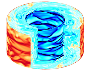
A three-dimensional annular centrifugal RB cell bounded by two independent-rotating concentric cylinders is considered, as shown in figure 1. The inner cylinder with radius  $R_i$ rotates about the $z$ axis at angular velocity $\varOmega _i$, and the outer cylinder with radius $R_o$ rotates at angular velocity $\varOmega _o$. The gap width between the two cylinders is $L=R_o-R_i$. The temperature difference between the hot outer cylinder and the cold inner cylinder is $\varDelta =\theta _{hot}-\theta _{cold}$. For the boundary, no-slip and isothermal conditions are applied at two cylinder surfaces; periodic boundary conditions are imposed on the velocity and temperature in the axial direction, and we take a section of height $H$ as the computational domain in DNS.

Figure 1. Schematic diagram of the flow configuration in the stationary reference frame, where  $R_o$, $R_i$ and $L$ are the inner radius of the outer cylinder, the outer radius of the inner cylinder, and the gap width between the two cylinders, respectively, and $H$ is the height of the cylindrical annulus in the computational domain of DNS. The outer cylinder rotates at angular velocity $\varOmega _o$, and the inner cylinder rotates at angular velocity $\varOmega _i$. Here, $\theta _{hot}$ and $\theta _{cold}$ are the temperatures of the outer and inner walls.
2.1. Governing equations of the flow
The system is at a rotating frame with angular velocity  $\varOmega _c$, and the buoyancy is induced by the centrifugal force $(\varOmega _cr+u_{\varphi })^2/r$. The motion of the flow is governed by the non-dimensional Oberbeck–Boussinesq equations under the cylindrical coordinate system $(r,\varphi,z)$ (Jiang et al. Reference Jiang, Zhu, Wang, Huisman and Sun2020; Wang et al. Reference Wang, Jiang, Liu, Zhu and Sun2022a):
 \begin{gather} \left.\begin{gathered} \boldsymbol{\nabla}\boldsymbol{\cdot}\boldsymbol{u}=0,\\ \frac{\partial\boldsymbol{u}}{\partial t}+\boldsymbol{u}\boldsymbol{\cdot} \boldsymbol{\nabla u}={-}\boldsymbol{\nabla} p-Ro^{{-}1}\,\boldsymbol{e}_{z} \times\boldsymbol{u}+\sqrt{\frac{Pr}{Ra}}\,\nabla^2\boldsymbol{u}-\theta\,\frac{2(1-\eta)}{1+\eta} \left(1+\frac{2u_\varphi}{Ro^{{-}1}\,r}\right)^2\boldsymbol{r},\\ \frac{\partial \theta}{\partial t}+\boldsymbol{u}\boldsymbol{\cdot} \boldsymbol{\nabla} \theta=\sqrt{\frac{1}{Ra\,Pr}}\,\nabla^2 \theta, \end{gathered}\right\} \end{gather}
where  $\boldsymbol {u}=(u_r,u_\varphi,u_z)$ is the velocity vector, $\theta \in [0,1]$ is the temperature, $p$ is the pressure, $\boldsymbol {e}_z$ is the unit vector along the axial direction, and $\eta =R_i/R_o$ is the radius ratio. Scaled quantities, including $L=R_o-R_i$ for length, $\varDelta$ for temperature, $U=\sqrt {\alpha \varDelta \varOmega _c^2({(R_i+R_o)}/{2})L}$ for velocity, and $L/U$ for time, are used to non-dimensionalize the governing equation, where $\alpha$ is the coefficient of thermal expansion of the fluid. Here, $\varOmega _c$ is the rotational speed of the rotating reference frame, and we suppose it to represent the strength of centrifugal buoyancy, as reflected in the expression of free-fall velocity $U$. In our system, considering both physical meaning and simplicity, we set $\varOmega _c=(\varOmega _i+\varOmega _o)/2$. It is a good estimate for free-fall velocity when shearing is relatively small, which means $\varOmega _i-\varOmega _o\ll \varOmega _c$; when shearing is strong enough and dominates the flow, buoyancy contributes little and can be neglected, which will be discussed later, in § 3. Therefore, the selected $\varOmega _c$ is reasonable in most of the parameter space. Under that rotating frame, the inner cylinder rotates at non-dimensional angular velocity $\varOmega =(\varOmega _i-\varOmega _c)L/U$, and the outer cylinder rotates at $-\varOmega$.
Three non-dimensional parameters are generated through non-dimensionalization: the Rayleigh number (measuring the buoyancy-driving strength)  $Ra$, the inverse Rossby number (measuring Coriolis effects) $Ro^{-1}$ and the Prandtl number (fluid property) $Pr$, expressed as
 \begin{equation} \left.\begin{gathered} Ra=\frac{(UL)^2}{\nu\kappa}=\frac{\alpha\varDelta\varOmega_c^2\,\dfrac{R_i+R_o}{2}\,L^3}{\nu\kappa},\\ Ro^{{-}1}=\frac{2\varOmega_cL}{U}=2\left(\frac{\alpha\varDelta(R_i+R_o)}{2L}\right)^{{-}1/2},\\ Pr=\frac{\nu}{\kappa}, \end{gathered}\right\} \end{equation}
where  $\nu$ is the kinematic viscosity, and $\kappa$ is the thermal diffusivity of the fluid. Therefore, there are five independent control parameters in the system: the Rayleigh number $Ra$, the inverse Rossby number $Ro^{-1}$, the Prandtl number $Pr$, the rotational speed difference of two cylinders $\varOmega =(\varOmega _i-\varOmega _c)L/U$, and the radius ratio $\eta$. Moreover, since the system can also be regarded as a TC system with radial buoyancy, the Taylor number $Ta$ can be defined as
 \begin{equation} Ta=\frac{(1+\eta)^4}{64\eta^2}\,\frac{(R_o-R_i)^2(R_i+R_o)^2(\varOmega_i-\varOmega_o)^2}{\nu^2}=\frac{(1+\eta)^6}{16\eta^2(1-\eta)^2}\,\frac{\varOmega^2\,Ra}{Pr}. \end{equation}
Therefore,  $Ta$ is not an independent control parameter in our system, proportional to $Ra$ and $\varOmega ^2$. The Richardson number $Ri$, measuring the ratio between buoyancy and shear driving, can also be calculated by the ratio of characteristic buoyancy velocity and characteristic shearing velocity:
 \begin{equation} Ri=\frac{U^2}{(\varOmega_i-\varOmega_c)^2R_i^2}=\left(\frac{1-\eta}{\eta}\right)^2\varOmega^{{-}2}. \end{equation}
As we can see, the non-dimensional rotational speed difference  $\varOmega$ can represent the strength of shear relative to buoyancy.
In addition, two key response parameters are the Nusselt numbers measuring the efficiency of heat transport and momentum transport, given by the ratio of radius-independent currents to the currents in laminar and non-vortical cases, respectively (Eckhardt et al. Reference Eckhardt, Grossmann and Lohse2007; Wang et al. Reference Wang, Jiang, Liu, Zhu and Sun2022a), as  $Nu_h=J^\theta /J^\theta _{lam}$, $Nu_\omega =J^\omega /J^\omega _{lam}$. The Nusselt numbers and how they respond to $Ra$ and $\varOmega$ will be discussed in § 3.
2.2. Linear stability analysis
Linear stability analysis is a good approach to studying the instability of the flow. At the stable state, the flow is laminar and non-vortical TC flow, and the heat is transferred by pure conduction. The azimuthal velocity  $V$ and temperature $\varTheta$ depend only on $r$, and the radial and axial velocities are zero. The functions of $V$ and $\varTheta$ are given by (Ali & Weidman Reference Ali and Weidman1990)
 \begin{equation} \left.\begin{gathered} V(r)=Ar+\frac{B}{r},\quad A={-}\frac{1+\eta^2}{1-\eta^2}\,\varOmega,\quad B=\frac{2r_i^2}{1-\eta^2}\,\varOmega,\\ \varTheta(r)=\frac{\ln(r/r_i)}{\ln(r_o/r_i)}, \end{gathered}\right\} \end{equation}
where  $r_i=\eta /(1-\eta )$ and $r_o=1/(1-\eta )$ are the non-dimensional radii of the inner and outer cylinders, respectively.
To perform LSA on this problem, we superimpose infinitesimal perturbations  $(u'_r,u'_\varphi,u'_z,p',\theta ')$ on the base flow state. After substituting the perturbation fields into (2.1), doing linearization, and expanding the perturbations into normal modes (Meyer et al. Reference Meyer, Yoshikawa and Mutabazi2015; Kang et al. Reference Kang, Meyer, Mutabazi and Yoshikawa2017),
 \begin{equation} (u'_r,u'_\varphi,u'_z,p',\theta')=(\widehat{u_r}(r),\widehat{u_\varphi}(r),\widehat{u_z}(r),\hat{p}(r),\hat\theta(r)) \exp(st+{\rm i}(n\varphi+kz)), \end{equation}
we obtain the following ordinary differential equations for  $r$-dependent normal mode quantities:
 \begin{gather} \left.\begin{gathered}
({\rm D}+r^{{-}1})\widehat{u_r}+{\rm
i}nr^{{-}1}\widehat{u_\varphi}+{\rm i}k\widehat{u_z}=0,\\
\left(s+\frac{{\rm
i}nV}{r}\right)\widehat{u_r}-\frac{2V}{r}\,\widehat{u_\varphi}=
-{\rm
D}\hat{p}+Ro^{{-}1}\,\widehat{u_\varphi}+\sqrt{\frac{Pr}{Ra}}\left(\nabla^2\widehat{u_r}-
\frac{\widehat{u_r}}{r^2}-\frac{2{\rm
i}n\widehat{u_\varphi}}{r^2}\right)\\
{}-\frac{2(1-\eta)}{(1+\eta)}\,r\left[\left(1+\frac{2V}{Ro^{{-}1}\,r}\right)^2\hat{\theta}+
\frac{4\varTheta}{Ro^{{-}1}\,r}\left(1+\frac{2V}{Ro^{{-}1}\,r}\right)\widehat{u_\varphi}\right],\\
\left(s+\frac{{\rm i}nV}{r}\right)\widehat{u_\varphi}\!+\!
\left({\rm
D}V\!+\!\frac{V}{r}\right)\widehat{u_r}={-}\frac{{\rm
i}n}{r}\,\hat{p}\!-\!Ro^{{-}1}\,
\widehat{u_r}+\sqrt{\frac{Pr}{Ra}}\left(\nabla^2\widehat{u_\varphi}-\frac{\widehat{u_\varphi}}{r^2}+\frac{2{\rm
i}n\widehat{u_r}}{r^2}\right),\\ \left(s+\frac{{\rm
i}nV}{r}\right)\widehat{u_z}={-}{\rm
i}k\hat{p}+\sqrt{\frac{Pr}{Ra}}\,\nabla^2\widehat{u_z},\\
\left(s+\frac{{\rm
i}nV}{r}\right)\hat{\theta}+({\rm
D}\varTheta)\widehat{u_r}=\frac{1}{\sqrt{Ra\,Pr}}\,\nabla^2\hat{\theta},
\end{gathered}\right\}
\end{gather}
\begin{gather} \left.\begin{gathered}
({\rm D}+r^{{-}1})\widehat{u_r}+{\rm
i}nr^{{-}1}\widehat{u_\varphi}+{\rm i}k\widehat{u_z}=0,\\
\left(s+\frac{{\rm
i}nV}{r}\right)\widehat{u_r}-\frac{2V}{r}\,\widehat{u_\varphi}=
-{\rm
D}\hat{p}+Ro^{{-}1}\,\widehat{u_\varphi}+\sqrt{\frac{Pr}{Ra}}\left(\nabla^2\widehat{u_r}-
\frac{\widehat{u_r}}{r^2}-\frac{2{\rm
i}n\widehat{u_\varphi}}{r^2}\right)\\
{}-\frac{2(1-\eta)}{(1+\eta)}\,r\left[\left(1+\frac{2V}{Ro^{{-}1}\,r}\right)^2\hat{\theta}+
\frac{4\varTheta}{Ro^{{-}1}\,r}\left(1+\frac{2V}{Ro^{{-}1}\,r}\right)\widehat{u_\varphi}\right],\\
\left(s+\frac{{\rm i}nV}{r}\right)\widehat{u_\varphi}\!+\!
\left({\rm
D}V\!+\!\frac{V}{r}\right)\widehat{u_r}={-}\frac{{\rm
i}n}{r}\,\hat{p}\!-\!Ro^{{-}1}\,
\widehat{u_r}+\sqrt{\frac{Pr}{Ra}}\left(\nabla^2\widehat{u_\varphi}-\frac{\widehat{u_\varphi}}{r^2}+\frac{2{\rm
i}n\widehat{u_r}}{r^2}\right),\\ \left(s+\frac{{\rm
i}nV}{r}\right)\widehat{u_z}={-}{\rm
i}k\hat{p}+\sqrt{\frac{Pr}{Ra}}\,\nabla^2\widehat{u_z},\\
\left(s+\frac{{\rm
i}nV}{r}\right)\hat{\theta}+({\rm
D}\varTheta)\widehat{u_r}=\frac{1}{\sqrt{Ra\,Pr}}\,\nabla^2\hat{\theta},
\end{gathered}\right\}
\end{gather}
where operators  $\textrm {D}=\textrm {d}/\textrm {d}r$ and $\nabla ^2=\textrm {D}^2+\textrm {D}/r-n^2/r^2-k^2$ are introduced for simplification. Here, $s$ is the temporal growth rate of perturbation, $n$ is the azimuthal mode number, and $k$ is the axial wavenumber. Due to the infinite axial length and $2{\rm \pi}$ period in the azimuthal direction, $k$ must be real and $n$ must be an integer. The boundary conditions of the perturbations are homogeneous:
 \begin{equation} \left.\begin{gathered}
\text{for}\ r=r_i,\quad
\widehat{u_r}=\widehat{u_\varphi}=\widehat{u_z}=\hat{p}=\hat\theta=0,\\
\text{for}\ r=r_o,\quad
\widehat{u_r}=\widehat{u_\varphi}=\widehat{u_z}=\hat{p}=\hat\theta=0.
\end{gathered}\right\}
\end{equation}
\begin{equation} \left.\begin{gathered}
\text{for}\ r=r_i,\quad
\widehat{u_r}=\widehat{u_\varphi}=\widehat{u_z}=\hat{p}=\hat\theta=0,\\
\text{for}\ r=r_o,\quad
\widehat{u_r}=\widehat{u_\varphi}=\widehat{u_z}=\hat{p}=\hat\theta=0.
\end{gathered}\right\}
\end{equation}
So the instability problem has been transformed into an eigenvalue problem, described by (2.7)–(2.8). This eigenvalue problem is solved by the Chebyshev spectral collocation method. Equation (2.7) are discretized on Chebyshev–Gauss–Lobatto collocation points with Chebyshev differentiation matrices. In our work, the number of collocation points ranges from  $200$ to $400$ for good convergence. Then the growth rate of perturbations $s$ becomes the eigenvalue of the generalized eigenvalue problems in the matrix form, and the corresponding perturbation normal modes are the eigenvectors. For certain parameters ( $Ra, Pr, Ro^{-1}, \varOmega, \eta$), the flow is stable if for all $(n, k)$, the growth rate $\sigma =\textrm {real}(s)$ is always negative, which means that all perturbation modes decay with time.
2.3. Direct numerical simulations
Direct numerical simulations (DNS) are performed using an energy-conserving second-order finite-difference code based on a Chebyshev-clustered staggered grid. The time stepping of the explicit terms is based on a fractional-step third-order Runge–Kutta scheme, and the implicit terms are based on a Crank–Nicolson scheme with a pressure correction step set following. For more details on the numerical schemes of the governing equations, we refer the reader to the literature (Verzicco & Orlandi Reference Verzicco and Orlandi1996; van der Poel et al. Reference van der Poel, Ostilla-Mónico, Donners and Verzicco2015; Zhu et al. Reference Zhu, Phillips, Spandan, Donners, Ruetsch, Romero, Ostilla-Mónico, Yang, Lohse and Verzicco2018).
Adequate resolutions are ensured for all simulations, and we have performed posterior checks of spatial and temporal resolutions to guarantee the resolution of all relevant scales. The ratios of maximum grid spacing  $\varDelta _g$ to the Kolmogorov scale estimated by the global criterion $\eta _K=(\nu ^3/\varepsilon )^{1/4}$, where $\varepsilon$ is the mean viscous dissipation rate via exact relation, and the Batchelor scale $\eta _B=\eta _K\,Pr^{-1/2}$ (Silano, Sreenivasan & Verzicco Reference Silano, Sreenivasan and Verzicco2010) are checked, as shown in the Appendix. Furthermore, the clipped Chebyshev-type clustering grids adopted in the radial direction ensure the spatial resolution within boundary layers, as at least $10$ grid points inside the thermal boundary layers. As for temporal resolution, we use the Courant–Friedrichs–Lewy (CFL) conditions and set $CFL\leq 0.7$ to guarantee the computational stability (Ostilla et al. Reference Ostilla, Stevens, Grossmann, Verzicco and Lohse2013; van der Poel et al. Reference van der Poel, Ostilla-Mónico, Donners and Verzicco2015; Zhang, Zhou & Sun Reference Zhang, Zhou and Sun2017). The simulations are run over enough time after the system has reached the statistically stationary state to obtain good statistical convergence. The relative difference of $Nu_h$ based on the first and second halves of the simulations is generally less than $1\,\%$. And for $Nu_\omega$, as its absolute value is small and close to $1$ in many weak shear cases, the relative difference is controlled generally less than $4\,\%$ under weak shear, and less than $2\,\%$ under strong shear. All those details are provided in the Appendix.
2.4. Other numerical details
In the present study, we consider the coupling effect of shear and buoyancy on the flow structure and heat and momentum transfer, that is,  $(Nu_h, Nu_\omega )=f(Ra,\varOmega )$. Therefore, referring to the results of our previous experiments and simulations of ACRBC (Jiang et al. Reference Jiang, Zhu, Wang, Huisman and Sun2020, Reference Jiang, Wang, Liu and Sun2022; Wang et al. Reference Wang, Liu, Zhou and Sun2022b), $Pr=4.3$ is taken for water at $40\,^{\circ }\textrm {C}$, and $\eta$ is set to be $0.5$. Considering the Boussinesq approximation, $\alpha \varDelta \ll 1$ is required. According to (2.2), we choose $\alpha \varDelta =6.67\times 10^{-3}$ and then $Ro^{-1}=20$, which is also in the parameter range of our previous experiments, corresponding to a temperature difference $\varDelta \approx 17.3\ \textrm {K}$ for water (Jiang et al. Reference Jiang, Zhu, Wang, Huisman and Sun2020, Reference Jiang, Wang, Liu and Sun2022). The non-Oberbeck–Boussinesq effect is not obvious at this temperature difference (Ahlers et al. Reference Ahlers, Brown, Araujo, Funfschilling, Grossmann and Lohse2006), and the Oberbeck–Boussinesq conditions are well satisfied. Meanwhile, considering the definition of $Ro^{-1}$, in the non-dimensional system, the rotational speed of the rotating reference frame is $\varOmega _cL/U=Ro^{-1}/2=10$.
As for instability, we focus on  $Ra\in [10^3,10^9]$ and $\varOmega \in [10^{-2},10]$, where positive $\varOmega$ means that the inner cylinder rotates at a faster angular velocity than the outer cylinder in the stationary reference frame. For example, $\varOmega =10$ corresponds to the state where the inner cylinder is rotating with the non-dimensional angular velocity $\omega =20$ and the outer cylinder is static in the stationary reference frame. The DNS for heat transfer analysis cover an $Ra$ range $[10^6,10^8]$ and a rotational speed difference $\varOmega$ range $[10^{-2},10]$.
3. Results and discussion
Previous studies have discussed or implied how the flow and heat transfer are at both ends of our parameter range. When  $\varOmega =0$, Jiang et al. (Reference Jiang, Zhu, Wang, Huisman and Sun2020) show that the flow will be quasi-two-dimensional at high $Ro^{-1}$ ( $\ge 10$), due to the constraint of the Taylor–Proudman theorem. The scaling law of heat transfer in this region follows the Grossmann–Lohse theory, with a power-law relationship $Nu\sim Ra^{0.27}$ in the classical regime. At the other end, $\varOmega =10$, with only the inner cylinder rotating, previous work (Leng et al. Reference Leng, Krasnov, Li and Zhong2021; Leng & Zhong Reference Leng and Zhong2022) implies that the shear is so strong that the flow is dominated by the TC vortex and the temperature behaves like a passive scalar. In this section, we will reveal how the flow undergoes such a large transformation, from the RB flow in the $r\varphi$ plane to the TC flow developed in the $rz$ plane.
3.1. Flow regimes
When increasing shear converts the flow from the RB flow to the TC flow, a stable regime is found on the way. To determine the boundaries of the stable regime, the approach of LSA is applied and the results are checked by DNS. As shown in figure 2(a), two unstable regimes are distributed on the two sides of the parameter domain, and a stable regime is located in the middle. The results of DNS agree well with the boundaries given by LSA, guaranteeing the validity of the stable regime. We denote the three regimes as the RB-dominated regime (Regime I), stable regime (Regime II) and TC-dominated regime (Regime III), with the shear strength increasing.

Figure 2. (a) Instability regimes divided by LSA (green lines) and checked by DNS (red circles and blue triangles) in the  $(Ra,\varOmega )$ parameter domain. Instantaneous temperature fields from DNS at $Ra=10^6$ and (b) $\varOmega =10^{-2}$ (Regime I), (c) $\varOmega =1$ (Regime II), and (d) $\varOmega =7$ (Regime III).
In the stable regime (Regime II), the typical instantaneous temperature field is illustrated in figure 2(c). The system is governed by steady laminar and non-vortical TC flow, as described by (2.5). In the other two regimes, the typical instantaneous temperature fields exhibit significant differences, depicted in figures 2(b) and 2(d). In Regime I, the flow is quasi-two-dimensional on the  $r\varphi$ plane. Plumes are detached from the boundary layers, move across the bulk region, and transfer heat to the other side. Several convection roll pairs are generated, the number depending on the radius ratio $\eta$ when there is no shear (Pitz et al. Reference Pitz, Marxen and Chew2017; Wang et al. Reference Wang, Jiang, Liu, Zhu and Sun2022a). In Regime III, the flow is three-dimensional, and the roll pairs, also called Taylor vortices, are mainly on the $rz$ plane, which can be seen clearly on the vertical $\varphi$ slice in figure 2(c). There are large differences among the flow structures in these three regimes. For a fixed $Ra$, as the shear increases from zero, the flow first stabilizes from a quasi-two-dimensional RB flow into a laminar flow, and then destabilizes into a three-dimensional flow similar to the TC flow. It is worth noting that as $\eta =0.5$ in our system, the Richardson number is $Ri=\varOmega ^{-2}$, based on (2.4). Therefore, at high $Ra$, the stable regime is located at $Ri\sim O(1)$, which means that the buoyancy is of the same order as the shear; this is consistent with the transition region from buoyancy-dominated to shear-dominated obtained from previous work (Blass et al. Reference Blass, Zhu, Verzicco, Lohse and Stevens2020; Leng et al. Reference Leng, Krasnov, Li and Zhong2021).
The curves representing the marginal states between regimes contain important information. The boundary between Regimes I and II has a horizontal asymptote on the left side for  $\varOmega \rightarrow 0$, that is, the onset $Ra$ of the ACRBC at $\eta =0.5$. As $\varOmega$ increases, the instability of the flow is suppressed, and a stronger buoyancy force is required to drive the convection. The critical Rayleigh number $Ra_c$ of the marginal state grows faster and faster with increasing $\varOmega$, and finally, when $\varOmega$ exceeds a certain value (approximately $0.6$ with our parameter settings), the flow is always stable no matter how much the Rayleigh number increases in our parameter range. According to the marginal-state curve in figure 2(a), there may also exist a vertical asymptote for $Ra\rightarrow \infty$. With the participation of the shear, the flow instability problem is different from the onset of the RB convection. For the onset $Ra$ of the ACRBC without shear, there exists a perturbation energy balance between the work performed by the buoyancy and the energy dissipation by the fluid viscosity; when the shear is imposed, the movement of the boundaries changes the balance. In addition, we notice that for the sheared classical rectangular RB system, the flow does not become stable with increasing shear (Blass et al. Reference Blass, Zhu, Verzicco, Lohse and Stevens2020). This indicates that the effect of curvature and the rotation in sheared ACRBC may also contribute to the stabilization of the flow. We will discuss the physics of the instability between Regimes I and II in depth in § 3.2.
Moreover, the straight boundary between Regimes II and III seems to behave differently. On this boundary,  $Ta$ is much larger than $Ra$: according to (2.3), when $Ra=10^3$, $Ta\approx 1\times 10^5$. Therefore, the marginal-state curve between Regimes II and III is similar to the line given by Rayleigh's inviscid criterion (Ali & Weidman Reference Ali and Weidman1990; Drazin & Reid Reference Drazin and Reid2004; Yoshikawa et al. Reference Yoshikawa, Nagata and Mutabazi2013), with the thermal effect enhancing the instability slightly. As the instability of TC flow with radial temperature difference has been discussed widely (Ali & Weidman Reference Ali and Weidman1990; Yoshikawa et al. Reference Yoshikawa, Nagata and Mutabazi2013, Reference Yoshikawa, Meyer, Crumeyrolle and Mutabazi2015; Kang et al. Reference Kang, Yang and Mutabazi2015; Meyer et al. Reference Meyer, Yoshikawa and Mutabazi2015), we focus mainly on the instability in Regimes I and II in the following discussion.
3.2. Instability
3.2.1. Mode analysis
To investigate the effect of shear on the flow and how the stable regime arises, we begin with linear instability. In Regime I, the flow is unstable, and each pair of azimuthal and axial wavenumbers  $(n,k)$ is associated with a perturbation mode of a growth rate $\sigma$. We notice that for every $n$,
$n$,  $\sigma$ reaches a maximum at $k=0$, corresponding to the quasi-two-dimensional flow characteristic in Regime I, that the flow is limited on the $r\varphi$ plane. Therefore, only $k=0$ is considered in subsequent analysis on Regime I.
To investigate how shear influences the flow instability, we analyse the growth rate  $\sigma$ as a function of the azimuthal wavenumber $n$ for increasing $\varOmega$ at $Ra=10^7$, and the results are plotted in figure 3(a). In the no-shear case $\varOmega =0$, $\sigma$ grows with $n$ quickly at first and then reaches a plateau. Modes of high azimuthal frequency $n\gtrsim 5$ are preferred, having a higher growth rate than the low azimuthal wavenumber modes. With the shear imposed, the growth rates of all modes decrease synchronously, while the high-frequency modes are suppressed more. This means that shear suppresses the growth of linear instability and further influences the generation of the convection flow. Meanwhile, perturbations with higher azimuthal frequency modes are suppressed more, and the dominated mode becomes the low-frequency mode gradually, as an increasing shear is imposed. Figure 3(b) demonstrates this trend. The azimuthal wavenumber of the main mode (the mode owning maximum growth rate $\sigma$) $n_{main}$ decreases from $15$ to $1$ with the increasing shear. When the flow approaches the marginal state, $n_{main}$ drops to $1$ and remains there. Figure 3(c) shows, at the marginal state, how the critical azimuthal number $n_c$ changes with the critical Rayleigh number $Ra_c$. At the no-shear state, which is the left asymptote in figure 2(a), $n_c=5$, giving the mode of five roll pairs. As the Rayleigh number and the shear increase, $n_c$ drops from $5$ to $1$, and remains at high Rayleigh number $(Ra_c\geqslant 10^6)$. It is worth noting that in figure 2(a), the critical rotating difference $\varOmega _{cr}$ reaches a maximum near $Ra=10^6$ as well, and then the $\varOmega _{cr}$ required to stabilize the flow decreases slightly with increasing $Ra$. The slight decrease of $\varOmega _{cr}$ may be related to the fact that the critical azimuthal wavenumber reaches the minimum.

Figure 3. (a) Growth rate  $\sigma$ as a function of the azimuthal wavenumber $n$ for $\varOmega =0$, 0.1, 0.3, 0.5 and $0.57$, at $Ra=10^7$. The black dashed line denotes $\sigma =0$. (b) The azimuthal wavenumber of the main mode $n_{main}$ as a function of $\varOmega$, at $Ra=10^7$. (c) The critical azimuthal wavenumber $n_c$ as a function of the critical Rayleigh number $Ra_c$ at the marginal state.
The temperature and velocity eigenfunctions of certain modes normalized by the maximum temperature perturbations are illustrated in figure 4. For  $n=1$, there is only one hot–cold perturbation pair, while for $n=5$ there are five pairs. In all perturbation modes, the colder flow goes outwards from the inner side with a clockwise azimuthal velocity, in the direction opposite to the basic flow. When the system is under low shear, as shown in figure 4(a), the azimuthal motion of the flow is strong at the junction of the cold and hot flows, while relatively weak at the centre of cold and hot perturbations. Near the inner wall, two flows with opposing azimuthal velocities converge at the centre region of cold temperature perturbations. As a result of the mass conservation, the flow undergoes an outward deflection, thereby transporting the strong cold-temperature perturbations towards the outer wall. Similar structures exist extensively in the modes under various conditions, as illustrated in figures 4(b)–4(d). Comparing figures 4(b) and 4(a), as the shear becomes stronger, we notice that the cold and hot perturbations are more stretched azimuthally and are narrower radially, which is similar to the plumes in sheared RB convection (Goluskin et al. Reference Goluskin, Johnston, Flierl and Spiegel2014; Blass et al. Reference Blass, Zhu, Verzicco, Lohse and Stevens2020). In figure 4(b), a strong azimuthal velocity exists everywhere in the cold and hot flow, even in the centre region of the cold flow, different from the low-shear case. The main motion of the flow is in the azimuthal direction, which has a negative effect on heat transfer and the work done by buoyancy. Under stronger shear, it seems more difficult to transport heat from one side to the other side. Both larger dissipation and less work done by buoyancy depress the growth of the instability.

Figure 4. Eigenfunctions  $(\boldsymbol {u}', \theta ')$ of the unstable modes at corresponding conditions: (a) $Ra=10^6$, $\varOmega =0.1$, $n=1$; (b) $Ra=10^6$, $\varOmega =0.5$, $n=1$; (c) $Ra=10^6$, $\varOmega =0.5$, $n=5$; (d) $Ra=10^8$, $\varOmega =0.5$, $n=1$. The maximum temperature perturbation is set to be the same in all conditions, $|\theta '|_{max}=10^{-2}$. The velocity perturbation vectors are scaled by the maximum velocity magnitude of each, as $|\boldsymbol {u}'|_{max}$ equals (a) $7.3\times 10^{-3}$, (b) $4.0\times 10^{-3}$, (c) $4.2\times 10^{-3}$, (d) $4.0\times 10^{-3}$.
Moreover, for the modes of high azimuthal frequency under strong shear, more pairs occupy the azimuthal length  $2{\rm \pi}$, an example of which is shown in figure 4(c). The temperature perturbation pairs and flow roll pairs are denser, presenting a pattern that extends anticlockwise from the inside out. As can be expected, this mode has higher dissipation and more significant buoyancy work than the low azimuthal frequency mode $n=1$ in figure 4(b). In addition, we are interested in the instability case when moving to high Rayleigh numbers. A mode near the marginal state at $Ra=10^8$ is presented in figure 4(d). Interestingly, the perturbations exhibit a pronounced concentration within an exceedingly narrow annulus, located at approximately the intermediate radius of the system. Inside and outside of this annulus, both temperature and velocity perturbations are weak. As $Ra$ escalates, the annulus progressively diminishes in width, tending to converge to a certain radius, which may be associated with the limit of $\varOmega _{cr}$ for an infinitely great Rayleigh number.
3.2.2. Energy analysis
In order to get a comprehensive explanation of the instability in Regime I, we perform the energy analysis on perturbations. Multiply the velocity perturbations  $u'_r,u'_\varphi,u'_z$ by the linearized momentum equations in their respective directions, and take their summation. Then the kinetic energy equation of perturbations is obtained (Yoshikawa et al. Reference Yoshikawa, Nagata and Mutabazi2013, Reference Yoshikawa, Meyer, Crumeyrolle and Mutabazi2015; Meyer et al. Reference Meyer, Yoshikawa and Mutabazi2015):
 \begin{equation} \frac{{\rm d}K}{{\rm d}t}=W_{Ta}+W_{cB}-D_\nu, \end{equation}
where the kinetic energy  $K$, the power of inertial forces $W_{Ta}$, the power of centrifugal buoyancy $W_{cB}$ and the dissipation $D_\nu =\langle \varPhi \rangle$ are expressed as
 \begin{gather} \left.\begin{gathered}
K=\frac{1}{2}\,\langle|\boldsymbol{u}'|^2\rangle,\quad
W_{Ta}= \left\langle-u'_ru'_\varphi\left(\frac{{\rm
d}V}{{\rm d}r}-\frac{V}{r}\right)\right\rangle,\\
W_{cB}=\left\langle-\frac{2(1-\eta)ru'_r}{1+\eta}\left[\theta'\left(1+\frac{2V}{Ro^{{-}1}\,r}\right)^2+
\frac{4\varTheta
u'_\varphi}{Ro^{{-}1}r}\left(1+\frac{2V}{Ro^{{-}1}\,r}\right)\right]\right\rangle,\\
D_\nu=\sqrt{\frac{Pr}{Ra}}\left\langle
2\left[\left(\frac{\partial u'_r}{\partial r}\right)^2\!+\!
\left(\frac{1}{r}\,\frac{\partial
u'_\varphi}{\partial{r}}\!+\!\frac{u'_r}{r}\right)^2\!+\!
\left(\frac{\partial u'_z}{\partial
z}\right)^2\right]+\left[r\,\frac{\partial}{\partial r}
\left(\frac{u'_\varphi}{r}\right)+\frac{1}{r}\,\frac{\partial
u'_r}{\partial\varphi}\right]^2\right.\\
+\left.\left[\frac{1}{r}\,\frac{\partial
u'_z}{\partial\varphi}+\frac{\partial u'_\varphi}{\partial
z}\right]^2 +\left[\frac{\partial u'_r}{\partial
z}+\frac{\partial u'_z}{\partial r}\right]^2\right\rangle.
\end{gathered}\right\}
\end{gather}
\begin{gather} \left.\begin{gathered}
K=\frac{1}{2}\,\langle|\boldsymbol{u}'|^2\rangle,\quad
W_{Ta}= \left\langle-u'_ru'_\varphi\left(\frac{{\rm
d}V}{{\rm d}r}-\frac{V}{r}\right)\right\rangle,\\
W_{cB}=\left\langle-\frac{2(1-\eta)ru'_r}{1+\eta}\left[\theta'\left(1+\frac{2V}{Ro^{{-}1}\,r}\right)^2+
\frac{4\varTheta
u'_\varphi}{Ro^{{-}1}r}\left(1+\frac{2V}{Ro^{{-}1}\,r}\right)\right]\right\rangle,\\
D_\nu=\sqrt{\frac{Pr}{Ra}}\left\langle
2\left[\left(\frac{\partial u'_r}{\partial r}\right)^2\!+\!
\left(\frac{1}{r}\,\frac{\partial
u'_\varphi}{\partial{r}}\!+\!\frac{u'_r}{r}\right)^2\!+\!
\left(\frac{\partial u'_z}{\partial
z}\right)^2\right]+\left[r\,\frac{\partial}{\partial r}
\left(\frac{u'_\varphi}{r}\right)+\frac{1}{r}\,\frac{\partial
u'_r}{\partial\varphi}\right]^2\right.\\
+\left.\left[\frac{1}{r}\,\frac{\partial
u'_z}{\partial\varphi}+\frac{\partial u'_\varphi}{\partial
z}\right]^2 +\left[\frac{\partial u'_r}{\partial
z}+\frac{\partial u'_z}{\partial r}\right]^2\right\rangle.
\end{gathered}\right\}
\end{gather}
The angle brackets  $\langle {\cdot }\rangle$ denote the average over the whole space $r$,
$r$,  $\varphi$ and $z$. A mode is stable if the right-hand side of (3.1) is negative. The kinetic energy generation terms $W_{Ta},W_{cB},D_\nu$ normalized by the kinetic energy $K$ are illustrated in figure 5 as functions of $\varOmega$ at $Ra=10^6$ and $10^8$. As all terms are normalized by the averaged kinetic energy $K$, the left-hand side of (3.1), $\textrm {d}K/\textrm {d}t$, is twice the growth rate, derived from (2.6). As shown in figure 5(a), $Ra=10^6$ and $n=1$, with $\varOmega$ increasing, the power of centrifugal buoyancy $W_{cB}$ decreases and the dissipation term $D_\nu$ increases slightly, in line with our analysis of the modes in figure 4. The largest change is in the inertial force action term, $W_{Ta}$, which is zero under no shear, but its magnitude increases rapidly as $\varOmega$ increases. According to the formula for $W_{Ta}$ in (3.2), this term is closely related to the shear action. When the system reaches the marginal state, three energy generation terms exhibit equilibrium. The presence of $W_{Ta}$ constitutes the primary differentiating factor between the flow instability with shear and the flow instability without shear.

Figure 5. Variation of energy generation terms  $-W_{Ta}$, $D_\nu$, $W_{cB}$, and the growth rate of kinetic energy ${\textrm {d}K}/{\textrm {d}t}$ with $\varOmega$, at conditions (a) $Ra=10^6$, $n=1$, (b) $Ra=10^6$, $n=5$, (c) $Ra=10^8$, $n=1$. All terms are normalized by $K$. The modes in the light orange regions are unstable, while those in the blue regions are stable.
The energy analysis method can also explain the reasons behind the greater suppression of high-azimuthal-frequency modes in comparison to low-frequency modes to a certain degree. Figure 5(b) shows the variation of energy generation terms under  $Ra=10^6$, $n=5$. At $\varOmega =0$, the centrifugal buoyancy term $W_{cB}$ is much larger than the dissipation, injecting a lot of energy into the development of the instability. However, with shear imposed, both $-W_{Ta}$ and $D_\nu$ rise quickly, while the buoyancy term $W_{cB}$ drops faster than in the low-frequency mode $n=1$. This reflects the strong suppression of the high-frequency modes by shear. Unlike the low-frequency mode in figure 5(a), the dissipation term $D_\nu$ plays a more important role, increasing significantly with shear, which is closely related to the tight distribution of velocity perturbation rolls. Therefore, although the high-frequency mode offers a high growth rate at no shear, it reaches the marginal state earlier as the shear increases.
At high  $Ra$, the dissipation term decreases at first with increasing shear, as illustrated in figure 5(c). The buoyancy terms drop more than the mode at $Ra=10^6$, as the perturbations are concentrated in a narrow annulus and the azimuthal motion occupies more kinetic energy. Meanwhile, we notice that at the marginal state, it is still a balance of three items, $W_{Ta}, W_{cB}, {D_\nu }$, which can be observed further at higher $Ra=10^{13}$. Therefore, the limit of instability as the Rayleigh number tends to infinity cannot be explained by an inviscid solution, since the dissipation term $D_\nu$ is not negligible.
Moreover, at  $Ra=10^6$, the distributions of energy generation terms $w_{Ta}, w_{cB}, \varPhi$ are compared under different shear strengths with the azimuthal wavenumber $n=1$, as shown in figure 6. The densities of energy generation terms are also normalized by $K$. By comparing figures 6(b) and 6(f), one can see that the power of the inertial term $w_{Ta}$ increases substantially with the enhancement of shear. (Note that the scales of the colour bars in these two plots are different.) Negative $w_{Ta}$ is derived from the rightward deflection of outward or inward flow ( $u'_ru'_\varphi <0$), while the positive part comes mainly from the limit of mass conservation near the boundary, and occurs at the junction of cold and hot currents. As for the buoyancy power $w_{cB}$, the increase of shear amplifies its maximum intensity while making it more concentrated in distribution, as the cold and hot perturbations are more stretched azimuthally. Dissipation term $\varPhi$ occurs mainly near the boundary and the regions with opposing flows of cold and hot currents, where a strong velocity gradient exists. As shear increases, $\varPhi$ increases significantly at the region where two flows meet, contributing to a final increase of $D_\nu$. These qualitative interpretations are in relatively good agreement with the curves in figure 5(a).

Figure 6. Distributions of perturbations (a,e)  $(\boldsymbol {u}',\theta ')$ and the densities of energy-generation terms (b,f) $w_{Ta}$, (c,g) $w_{cB}$, and (d,h) $\varPhi$, under different shears (a–d) $\varOmega =0.1$, and (e–h) $\varOmega=0.5$, when $Ra=10^6$, $n=1$. All the densities of energy-generation terms are normalized by the averaged kinetic energy $K$. Note that the scales of $w_{Ta}$ in (b,f) are different.
3.3. Heat and momentum transfer
In this subsection, we focus on both heat and momentum transport efficiency, and discuss their behaviours in different regimes. Under the dimensionless formulation, the heat transfer efficiency and the momentum transfer efficiency are measured by two Nusselt numbers,  $Nu_h$ and $Nu_\omega$, defined as the ratios of the corresponding currents of the system to the currents in the laminar and non-vortical flow cases (Eckhardt et al. Reference Eckhardt, Grossmann and Lohse2007; Wang et al. Reference Wang, Jiang, Liu, Zhu and Sun2022a):
 \begin{equation} \left.\begin{gathered} Nu_h=\frac{\sqrt{Ra\,Pr}\,\langle u_r\theta\rangle_{t,\varphi,z}-\partial_r\langle\theta\rangle_{t,\varphi,z}}{(r\ln(\eta))^{{-}1}},\\ Nu_\omega=\frac{r^3[Ra/Pr\,\langle u_r\omega\rangle_{t,\varphi,z}-\sqrt{Ra/Pr}\,\partial_r\langle\omega\rangle_{t,\varphi,z}]}{2B}, \end{gathered}\right\} \end{equation}
where  $\omega =u_\varphi /r$ is the angular velocity of the fluid, and $B$ is the parameter of the base flow defined in (2.5). The variations of the two Nusselt numbers with the shear strength $\varOmega$ under different Rayleigh numbers are illustrated in figure 7. The different regimes in the figure are distinguished using different background colours. As the Taylor number is much larger than $Ra$ in Regime III ( $Ta=2.65\times 10^9$ at $Ra=10^7$, $\varOmega =10$, calculated from (2.3)), the flow is too drastic and computationally expensive, so we calculate only the cases with $Ra = 10^6$ in the TC-dominated regime.

Figure 7. Variation of (a)  $Nu_h$ and (b) $Nu_\omega$ with $\varOmega$, at $Ra=10^6$, $10^7$ and $10^8$.
In Regime I, as the imposed shear increases,  $Nu_h$ decreases slowly at first and then rapidly when $\varOmega >0.3$. The curves of different $Ra$ behave in a similar trend. The heat transfer efficiency $Nu_h$ increases with $Ra$ in Regime I, but as the shear increases and flow turns stable, $Nu_h$ values under different $Ra$ all drop to $1$. These results are similar to the results in the sheared rectangular RB cell (Blass et al. Reference Blass, Zhu, Verzicco, Lohse and Stevens2020), where the heat transfer is also first depressed by shear. However, in a sheared rectangular RB cell, shear cannot turn the flow laminar. For momentum transfer, we notice that the system gives a negative $Nu_\omega$ under a weak shear, which means that the large-scale circulation (LSC) in the RB convection pushes the two cylinders to rotate relative to each other. According to the definition of $Nu_\omega$, when there is no relative rotation between two cylinders, LSC also imposes shear stress to the wall, and $Nu_\omega$ is negative infinity. Also, $Nu_\omega$ increases quickly as $\varOmega$ increases, and the growth trend slows down when its value is close to $1$. Similar to the heat transfer, a larger $Ra$ gives a stronger torque.
In Regime II, the flow field is laminar, described by (2.5). Both  $Nu_h$ and $Nu_\omega$ equal $1$. As $\varOmega$ increases, the system reaches the marginal state between Regimes II and III. If the buoyancy is not considered, then at high $Ta$, the marginal-state curve of Taylor instability is close to the solution given by Rayleigh inviscid theory (Drazin & Reid Reference Drazin and Reid2004), which gives $\varOmega =6$. Considering the buoyancy, the instability is strengthened and the flow at $\varOmega =6$ gives a heat transfer efficiency close to $Nu_h$ under weak shear. Meanwhile, $Nu_\omega$ remains almost unchanged, which means that the flow driven by buoyancy is hard to mix in the angular velocity profile. As the shear strength continues to increase, the heat transfer is enhanced more, and the momentum transfer increases gradually as well. It is suggested that this regime appears in a similar system with gravity-driven buoyancy, where the system is controlled mainly by the Taylor vortex, and temperature acts as a passive scalar (Leng et al. Reference Leng, Krasnov, Li and Zhong2021). To check if this idea is also valid in our system, we perform another set of simulations under the same conditions, where the velocity is decoupled from temperature (buoyancy not considered) and the temperature really acts as a passive scalar. The comparison of the two is displayed in figure 8(a). As there is no buoyancy, the system is still stable at $\varOmega =6$, but then it behaves almost the same as the velocity–temperature coupled system, at $\varOmega =6.5$ in the figure. Therefore, in most of Regime III, the temperature can be regarded as a passive scalar in our system; it is the shear that dominates the flow.

Figure 8. (a) Variation of  $Nu_h$ with $\varOmega$ in Regime III, for the cases where the temperature and velocity are coupled (purple line) and uncoupled (red line), with $Ra=10^6$. (b) Variation of $|\gamma |$ with $\varOmega$ at $Ra=10^6, 10^7, 10^8$. In Regime I $\gamma <0$, and in Regime III $\gamma >0$.
The exact relation gives us an interesting perspective to understand the relation between  $Nu_h$ and $Nu_\omega$. Derived from the kinetic energy balance equation, the exact relation represents the energy balance between buoyant energy injection, shear energy injection and mechanical dissipation. In the dimensional form, referring to derivation from Eckhardt et al. (Reference Eckhardt, Grossmann and Lohse2007) and Wang et al. (Reference Wang, Liu, Zhou and Sun2022b), if we assume $\langle \alpha \theta (\varOmega _c+u_\varphi /r)^2ru_r\rangle _{V,t}=C\alpha \varOmega _c^2\langle ru_r\theta \rangle _{V,t}$, then the exact relation of our system is
 \begin{equation} \varepsilon-\varepsilon_{lam}=\nu^{3}L^{{-}4}[\sigma_r^{{-}2}\,Ta\,(Nu_\omega-1)+C\,f(\eta)\,Pr^{{-}2}\,Ra\,(Nu_h-1)], \end{equation}
where  $\varepsilon =\nu \langle (\partial _iu_j+\partial _ju_i)^2\rangle _{V,t}$ is the mean energy dissipation rate, $\varepsilon _{lam}$ is the mean energy dissipation rate of the laminar and non-vortical flow, $\sigma _r=(1+\eta )^4/16\eta ^2$ is the quasi-Prandtl number, and $f(\eta )={2(\eta -1)}/{((1+\eta )\ln (\eta ))}$ is a correction factor. In Regime I, $u_\varphi /r\ll \varOmega _c$, we have $C\approx 1$. In Regime III, the flow is dominated by shear; therefore, referring to the angular velocity profile of the TC flow (Grossmann et al. Reference Grossmann, Lohse and Sun2016), $C$ is still of the order $O(1)$.
The terms on the right-hand side of (3.4) represent the energy injection by the wall shear and the buoyancy, respectively. The TC flow considers the first term, while the RB convection concentrates on the second. In Regime I, as  $Nu_h>1$ and $Nu_\omega <1$, only buoyancy provides energy for turbulent dissipation, while the wall motion consumes energy instead. In Regime III, buoyancy and shear provide energy to the fluid together. Moreover, considering the ratio of the two terms, we can verify the dominant regimes of the flow. The ratio $\gamma$ can be simplified by taking $\eta =0.5$, $Pr=4.3$ and $C\approx 1$:
 \begin{equation} \gamma=\frac{\sigma_r^{{-}2}\,Ta\,(Nu_\omega-1)}{C\,f(\eta)\,Pr^{{-}2}\,Ra\,(Nu_h-1)}\approx31.79\,\varOmega^2\,\frac{Nu_\omega-1}{Nu_h-1}, \end{equation}
where  $Ta/Ra$ is simplified using (2.3). How $\gamma$ varies with $\varOmega$ is shown in figure 8(b). In Regime I, $\gamma <0$; in Regime II, $\gamma$ is not calculated as both terms are zero; in Regime III, $\gamma >0$. When the system is under weak shear, such as $\varOmega =10^{-2}$, a very small fraction of the energy is consumed by shearing. As $\varOmega$ increases, more energy is transferred out of the system by the wall motion, as $|\gamma |$ grows approximately linearly with $\varOmega$ in logarithmic coordinates. At the point near Regime II, $\varOmega =0.5$, approximately half of the energy injected by buoyancy is consumed by the wall shear. Such a large percentage of energy consumption may be responsible for bringing the system to a stable state. Crossing Regime II into Regime III, $\gamma \gg 1$, the energy input by the wall shear is much more than the energy injection of the buoyancy. As $\varOmega$ increases, the dominance of shear is reinforced. Additionally, the data of the buoyancy-dominated part in Regime III ( $\varOmega =6$) is not given in figure 8(b), because the accuracy of $\gamma$ is difficult to guarantee as $Nu_\omega$ is very close to $1$. The factor in front of the ratio of the Nusselt numbers, $31.79\,\varOmega ^2$, is large, therefore it is hard for the buoyancy-driven flow ( $|\gamma |<1$) to influence $Nu_\omega$. From an alternative perspective, this can be attributed to the fact that the energy difference induced by angular velocity difference is much larger than the energy difference induced by density difference since the density variation is limited as $\alpha \varDelta \ll 1$.
3.4. Flow structures
To further investigate the dynamics behind the behaviours of heat and momentum transfer, we focus on the evolution of the flow structures. As the flow is stable in Regime II, the typical two-dimensional slices of temperature and angular velocity fields for Regimes I and III are visualized in figures 9 and 11, respectively. Next, we will explore and analyse the flow structures of the systems in Regimes I and III sequentially, to figure out how heat transfer is inhibited and facilitated, and how the system is stabilized.

Figure 9. Typical snapshots of (a–d) the instantaneous temperature  $\theta$, and (e–f) the angular velocity $\omega =u_\varphi /r$, at $\varOmega =0, 0.1, 0.3, 0.5$ in Regime I. Here, $Ra=10^6$.
3.4.1. Regime I
In Regime I, the flow is quasi-two-dimensional under a large inverse Rossby number,  $Ro^{-1}=20$. Therefore, two-dimensional slices on the $r\varphi$ plane are taken for the temperature and angular velocity fields under different $\varOmega$ at $Ra=10^6$, and the visualizations are displayed in figure 9. Without shear, four pairs of convection rolls are formed, which can be observed clearly in the temperature and angular velocity snapshots. Due to the effect of Coriolis force, hot plumes detached from the outer cylinder turn right when rising, therefore one roll pair consists of a bigger roll on the right of the hot plume and a smaller roll on the left. This effect also results in the zonal flow in annular centrifugal RB convection, which is explained well by Jiang et al. (Reference Jiang, Zhu, Wang, Huisman and Sun2020) and Wang et al. (Reference Wang, Jiang, Liu, Zhu and Sun2022a). The flow structure of the system is stable, and the heat is transferred continuously through the plume with the LSC. Meanwhile, due to the asymmetry of the two rolls, the bigger roll takes more area and has a larger impact on the boundaries than the other roll, which pushes the inner cylinder to rotate anticlockwise and the outer cylinder to rotate clockwise. Hence once the boundary is rotating slowly, a negative $Nu_\omega$ is generated.
It is conceivable that the flow structure shifts continuously with shear enhancement. As  $\varOmega$ increases to $0.1$, there is a notable alteration in the flow structure, whereby the quantity of convection roll pairs exhibits a decline. Only two pairs can be observed, and each pair consists of a large roll covering nearly half of the annulus and a quite small roll. These can be seen especially clearly in the angular velocity field. It can be speculated that the shear of two boundaries stretches the plumes and promotes the azimuthal motion of the plume in the shear direction. The stretched plumes under shear are also observed in sheared RB convection (Goluskin et al. Reference Goluskin, Johnston, Flierl and Spiegel2014; Blass et al. Reference Blass, Zhu, Verzicco, Lohse and Stevens2020). The flow motion induced by shear is in the same direction as the motion induced by the Coriolis force, including that hot plumes turn anticlockwise near the inner cylinder, and cold plumes turn clockwise near the outer cylinder; hence the imposed shear increases the size of the large roll further. Meanwhile, the other roll becomes smaller. The number of roll pairs decreases as the system is not large enough to accommodate four roll pairs. Moreover, at this stage, the angular velocity of the fluid is still larger than the rotational speed of the boundary, and stronger than the angular velocity of the fluid without shear as well. This means, on the one hand, the azimuthal motion of the fluid is strengthened by shear; on the other hand, the shear is not strong enough, and the azimuthal movement of the fluid driven by heat is still maintained. In the small rolls, the flow against the direction of boundary motion remains strong. Because of this, the basic convection structures, the LSC and plumes, are maintained, and the heat transfer is reduced by only a small fraction, approximately $6\,\%$ compared to the heat transfer at $\varOmega =0$.
As  $\varOmega$ continues to increase to $0.3$, one big roll covering near $3{\rm \pi} /2$ is generated. In this case, the number of convection roll pairs is hard to define, as the roll against the direction of boundary motion nearly disappears. Actually, though we can see two strong cold plumes in the temperature field, there is no fluid rotating anticlockwise near the outer cylinder; while near the inner cylinder, only two small pieces of fluid rotate clockwise, against the direction of boundary motion. For all the fluid in the system, $|\omega |\leq \varOmega$, fluid cannot rotate faster than the boundary wall, and $Nu_\omega$ turns positive but is still smaller than $1$. The rotating velocity of the boundaries exceeds the azimuthal velocity of the fluid induced by LSC. At this stage, the convection roll pairs are not maintained, while plumes remain working, transporting heat from one side to the other. Therefore, the heat transfer drops not too much but noticeably, reducing approximately $28\,\%$ compared to the heat transfer at $\varOmega =0$.
As  $\varOmega$ continues to increase to $0.5$, near the marginal state, the flow is close to the laminar and non-vortical flow, and the plumes disappear in the end. Some temperature fluctuations are observed in the temperature field, while the angular velocity fluctuations are hard to recognize. At this stage, the convection and heat transfer are highly suppressed. It is hard for plumes, as important carriers of heat transfer, to exist. The Nusselt number $Nu_h$ drops significantly, approximately $83\,\%$ compared to $Nu_h$ at $\varOmega =0$.
The averaged temperature and angular velocity profiles under different  $\varOmega$ are shown in figure 10. A uniform bulk temperature $\theta _c$ is observed for $\varOmega \le 0.3$, which deviates from the arithmetic mean temperature of the two boundaries $\theta _m=0.5$. The asymmetry temperature profiles without shear can be explained by the radially dependent gravity effects, and the bulk temperature $\theta _c$ depends on the radius ratio $\eta$, which are discussed by Wang et al. (Reference Wang, Jiang, Liu, Zhu and Sun2022a). The bulk temperature remains unchanged until $\varOmega$ exceeds $0.3$. As the shear increases, the uniform bulk temperature vanishes and the temperature profile gradually evolves toward a laminar and non-vortical flow profile (the dashed line). For the angular velocity profile, a stage similar to the bulk temperature is not found. At $\varOmega =0$, the averaged angular velocity is small as the asymmetry of the flow structure is not strong; as the shear is imposed, the averaged angular velocity varies from $\varOmega$ at the inner cylinder to $-\varOmega$ at the outer cylinder. It should be noted that when the shear is not strong (such as $\varOmega =0.1$), the two extrema of the profile occur inside the cell rather than on the boundaries, while for $\varOmega \ge 0.3$, the extrema of the profile move to the boundaries. As $\varOmega$ increases, the angular velocity profile gradually evolves towards a laminar flow profile as well. At $\varOmega =0.5$, it coincides almost exactly with the laminar and non-vortical flow profile, while the temperature profile still differs. Thus we can see that as shear is enhanced, the changes in the angular velocity profile are not synchronized with the changes in the temperature profile; the former tends to occur earlier, for the transition at either $\varOmega =0.3$ or $\varOmega =0.5$.

Figure 10. Radial distribution of azimuthally, axially and time-averaged (a) temperature  $\langle \theta \rangle _{t,\varphi,z}$ and (b) angular velocity $\langle \omega \rangle _{t,\varphi,z}$ profiles, for different $\varOmega$ in Regime I. Here, $Ra=10^6$. The dashed lines represent the profiles of the laminar and non-vortical flow.
3.4.2. Regime III
In Regime III, though the flow is three-dimensional, the main structure is on the  $rz$ plane (Grossmann et al. Reference Grossmann, Lohse and Sun2016). Therefore, two-dimensional slices are taken for the temperature and angular velocity fields, illustrated in figure 11. At $\varOmega =6$, for which the inviscid TC system without buoyancy is at the marginal state, the flow shows a classical RB temperature field with a typical LSC. However, the angular velocity distribution is still almost laminar and non-vortical, though convection occurs. As explained in § 3.3, the convection driven by heat makes it hard to transfer angular momentum at large $\varOmega$. With $\varOmega$ increasing, the flow becomes more turbulent, with the angular velocity field better mixed, and the plumes get thinner, meaning that the transport efficiency is enhanced. At this stage, because the temperature acts as a passive scalar, the temperature fields and the angular velocity fields are highly relevant, which can be seen roughly by the highly similar plume morphology.

Figure 11. Typical snapshots of the instantaneous (a–d) temperature  $\theta$ and (e–h) angular velocity $\omega =u_\varphi /r$, at $\varOmega =6, 7, 8.5, 10$ in Regime III. Here, $Ra=10^6$. The corresponding Taylor numbers are $Ta=9.54\times 10^7$, $1.30\times 10^8$, $1.91\times 10^8$, $2.65\times 10^8$, respectively.
The averaged temperature and angular velocity profiles of Regime III are shown in figure 12. A uniform bulk temperature is observed for all the cases, both buoyancy-dominant ( $\varOmega =6$) and shear-dominated. Interestingly, this temperature does not change with $\varOmega$, but is different from the arithmetic mean temperature $\theta _m=0.5$ and the bulk temperature in Regime I. As $\varOmega$ increases, the profile becomes sharper at the two boundaries, which also implies an improved efficiency of heat transfer. The angular velocity profile is in line with the laminar and non-vortical profile at $\varOmega =6$, then transits to a turbulent profile as the Taylor number increases. At $\varOmega =10$, the outer cylinder is at rest, and the Taylor number is $Ta=2.65\times 10^8$, therefore the system is still in the classical regime of the TC flow (Ostilla-Mónico et al. Reference Ostilla-Mónico, van der Poel, Verzicco, Grossmann and Lohse2014b; Grossmann et al. Reference Grossmann, Lohse and Sun2016); the shear-dominated flow in Regime III behaves similarly to the TC flow.

Figure 12. Radial distribution of azimuthally, axially and time-averaged (a) temperature  $\langle \theta \rangle _{t,\varphi,z}$ and (b) normalized angular velocity $\langle \omega \rangle _{t,\varphi,z}/\varOmega$ profiles, for different $\varOmega$ in Regime III. Here, $Ra=10^6$. The dashed lines represent the profiles of the laminar and non-vortical flow.
4. Conclusion
In the present study, we investigate the evolution of the flow regimes in an annular centrifugal Rayleigh–Bénard (RB) system with increasing imposed shear, which is represented by the angular velocity difference between the inner and outer cylinders,  $\varOmega$. At first, $Ri\ll 1$ under weak shear, the flow is buoyancy-dominated and manifests itself as quasi-two-dimensional convection on the $r\varphi$ plane. As $\varOmega$ increases, the convection and heat transfer are depressed, and the flow finally turns to stable laminar and non-vortical flow. Through linear instability analysis, we notice that the marginal state depends on both $Ra$ and $\varOmega$, formed by the energy balance among viscous dissipation, the work of buoyancy, and the work of inertial terms. At low $Ra\sim 10^3$, the marginal state depends mainly on $Ra$, and only a weak shear is required to stabilize the flow. At high $Ra\ge 10^6$, the marginal state seems insensitive to $Ra$, locating at $Ri=\varOmega ^{-2}\sim O(1)$. In the parameter region $Ra\in [10^6,10^8]$, as shear increases, the growth rate of the instability is suppressed and the low azimuthal frequency modes become the main mode. Similarly, the heat transfer efficiency $Nu_h$ is also depressed gradually, and the number of roll pairs decreases as the shear enhances the asymmetry between the two opposing rolls and enlarges the bigger one. The plumes are stretched by the shear, and the temperature perturbations are also stretched in LSA. The LSA and DNS give many comparable findings.
With the continued enhancement of shear, the flow becomes unstable again, but this time the flow is completely different from before. Initially, when the system has not crossed the marginal state derived by Rayleigh's inviscid theory for pure TC flow, the instability of the flow is driven by buoyancy, and the thermal convection occurs on the  $rz$ plane, similar to the classical RB convection. As $\varOmega$ increases and the centrifugal instability takes over, the flow quickly becomes shear-dominated, with the temperature acting as a passive scalar. At this moment, the flow is similar to the TC flow, still in the classical regime for our parameter sets.
On the whole, as the flow transits from an annular centrifugal RB convection to a radially heated TC flow of only the inner cylinder rotating, it passes through three regimes. Regime I is mainly buoyancy-dominated, and Regime II is the stable regime, while Regime III is mainly shear-dominated. There is an obvious dividing line between the three regimes, namely the marginal state of the instability. Furthermore, the energy analysis through the exact relation implies more information. In Regime I, the energy injected by buoyancy is consumed by both turbulent dissipation and wall shear. As the shear increases, more percentages of injected energy are taken by the wall motion, and near the marginal state, it takes approximately  $50\,\%$. Therefore, shear plays an important role in Regime I as well, diverting buoyant injections of energy and inhibiting the convection. Meanwhile, on the other end of the stable regime, buoyancy drives the flow at first. Convection is observed in the temperature profile while the angular velocity profile is still close to the profile in the laminar and non-vortical case. Near the marginal state, both shear and buoyancy are important, and the exact relation (3.4) is a good approach to analysing the flow characteristics.
The traditional RB system sheared by wall motion in a plane Couette flow is remarkably close to our system. Blass and Yerragolam have conducted a series of meaningful studies on this topic recently (Blass et al. Reference Blass, Zhu, Verzicco, Lohse and Stevens2020, Reference Blass, Tabak, Verzicco, Stevens and Lohse2021; Yerragolam et al. Reference Yerragolam, Stevens, Verzicco, Lohse and Shishkina2022a,Reference Yerragolam, Verzicco, Lohse and Stevensb). As shear increases from  $0$, the flow regime moves from the buoyancy-dominated regime, through the transitional regime, and finally into the shear-dominated regime. A non-monotonic progression of $Nu$ is observed as well, with a minimum in the transitional regime, where $Ri\sim 1$. These observations are consistent with ours, suggesting that the dominance of buoyancy or shear is a key factor in determining the flow state. Moreover, the coupling effects of buoyancy and shear on the heat transfer are also close between the two systems. However, due to the effect of curvature and rotation, the evolution of flow structures in the sheared ACRBC exhibits a lot of differences. The appearance of a stable regime is a very special finding. Meanwhile, because of the differences between the TC flow and the plane Couette flow, the flow in the shear-dominated regime is quite dissimilar. The similarities and differences between the sheared ACRBC and sheared RB are interesting points that deserve our future research.
The current system properly couples the TC flow with the RB convection through a pair of differential rotation centrifugal cylinders, and is a feasible approach to analyse the coupling effect of shear and buoyancy. Limited by the parameter space, there are plenty of questions to be explored further. In the region of high Rayleigh number, how does shear affect the  $Nu\sim Ra^\gamma$ scaling? Meanwhile, investigating the effect of other parameters on the stable region, including $Ro^{-1}$ and $Pr$, is also an interesting project. Moreover, some studies show that as the radius ratio $\eta$ increases and approaches $1$, the convection in the annulus system behaves more and more similarly to the convection between two planes (Pitz et al. Reference Pitz, Marxen and Chew2017; Wang et al. Reference Wang, Jiang, Liu, Zhu and Sun2022a). As we know, there is no stable regime for a sheared RB convection between two horizontal planes (Blass et al. Reference Blass, Zhu, Verzicco, Lohse and Stevens2020). The disappearance of the stable regime is an attractive phenomenon that deserves to be explored in the future.
Acknowledgements
We thank D. Lohse and H. Jiang for helpful discussions.
Funding
This work was supported by the National Natural Science Foundation of China under grant no. 11988102, and the New Cornerstone Science Foundation through the Xplorer Prize.
Declaration of interests
The authors report no conflict of interest.
Appendix. Simulation parameters
Simulation parameters are given in table 1.
Table 1. Simulation parameters. The columns display the Rayleigh number  $Ra$, the non-dimensional rotational speed difference $\varOmega$, the Taylor number $Ta$, the resolution employed, the maximum grid spacing $\varDelta _g$ compared with the Kolmogorov scale estimated by the global criterion $\eta _K=(\nu ^3/\varepsilon )^{1/4}$, the calculated Nusselt numbers $Nu_h$, $Nu_\omega$ and their relative difference of two halves $\epsilon _{Nu}=|(\langle Nu\rangle _{0-T/2}-\langle Nu\rangle _{T/2-T})/(Nu-1)|$, the aspect ratio $\varGamma =H/L$, and the reduced azimuthal domain $\phi _0$. Here, $\varepsilon$ is the mean energy dissipation rate calculated by (3.4) with $C\approx 1$. Note that the azimuthal resolution corresponds to the resolution of the segment. For example, $N_\varphi =768$ for $\phi _0=1/2$ means $768$ points for one half of the annulus.


 Open access