2.1. Drop impact experimental set-up

Our experimental set-up is adapted from the original set-up designed by Rozhkov et al. (Reference Rozhkov, Prunet-Foch and Vignes-Adler2002). A scheme of the set-up is shown in figure 1. In brief, we let a liquid drop fall on a solid cylindrical target of diameter slightly larger than that of the drop. The liquid drop is injected with a syringe pump and a needle positioned vertically with respect to the target. The impact velocity of the drop, $u_{0}$ , is set by the height of fall of the drop and the drop diameter, $d_{0}$ , is set by the needle diameter. Three different drop diameters ( $d_{0}=3.0,3.7$ and 4.8 mm) and two impact velocities ( $u_{0}=2.8$ and $4.0~\text{m}~\text{s}^{-1}$ ) are studied. In all experiments the ratio between the drop diameter and the target diameter is kept constant at 0.6. The Weber number, $\mathit{We}=({\it\rho}u_{0}^{2}d_{0})/{\it\gamma}$ , respectively the Reynolds number, $\mathit{Re}=({\it\rho}u_{0}d_{0})/{\it\eta}$ , where ${\it\gamma}$ is the fluid surface tension, ${\it\rho}$ its density and ${\it\eta}$ its viscosity, varies from 320 to 810, respectively from 8400 to 19 000. The target is an aluminium cylinder coated on the top with a glass lamella. The glass is rendered hydrophilic thanks to a plasma treatment with a plasma gun (Corona Surface Treater, Electro-Technic products), which suppresses the dewetting on the surface (Dhiman & Chandra Reference Dhiman and Chandra2010; Marengo et al. Reference Marengo, Antonini, Roisman and Tropea2011). A thin aluminium coaxial cylinder is added around the target as suggested by Villermaux & Bossa (Reference Villermaux and Bossa2011) in order to keep the sheet ejection angle equal to $90^{\circ }$ (with respect to the target axis) and obtain a horizontal and flat sheet. A vertical tube which runs from the needle to slightly above the target is mounted to avoid the effect of draughts and ensure a centred impact on the target. The target is mounted on a transparent Plexiglas floor lighted from below by a high-luminosity backlight (Phlox High Bright LED Backlights). The drop impact is recorded from the top with a weak angle using a Phantom V7.3 camera operating at 9708 pictures per second and with a resolution of $576~\text{pixels}\times 552~\text{pixels}$ . Side views are also recorded to check the flatness of the liquid sheet and to measure the impact velocity.

Figure 1.

Sketch of the drop impact experimental set-up. The experimental parameters are defined on the sketch.

2.2. Sheet thickness measurement

Measuring liquid film thicknesses at the micrometre-scale range is a problem of great interest for various industrial and academic applications. Different thickness measurement techniques have been developed over the last century. Tibiriçá et al. (Reference Tibiriçá, Do Nascimento and Ribatski2010) presented a comprehensive literature review of the experimental techniques developed to measure liquid film thicknesses ranging from micrometres to centimetres. Available methods can be classified based on the physical principles, acoustic, electrical or optical, involved in the measurements. In particular, numerous optical methods have been developed, including interferometry methods (Ohyama et al. Reference Ohyama, Endoh, Mikami and Mori1988), fluorescence intensity methods (Makarytchev, Langrish & Prince Reference Makarytchev, Langrish and Prince2001), methods based on imaging a diffusive liquid (Berhanu & Falcon Reference Berhanu and Falcon2013) or light absorption methods (Lilleleht & Hanratty Reference Lilleleht and Hanratty1961; Kim & Kim Reference Kim and Kim2005). Mouza et al. (Reference Mouza, Vlachos, Paras and Karabelas2000) compared two methods to measure liquid film thickness, a photometric technique based on the absorption of light passing through a layer of dyed liquid and a conductance measurement and found a very good agreement between these two methods. The authors also pointed out the advantages of optical methods based on light absorption over conductance method. Optical methods are non-intrusive, suitable for non-conducting fluids and can display sensitivity to thin films and high spatial resolution.

Here, we present a method to determine the thickness of liquid sheets, which is based on the light absorption by a dyed liquid. The method that we have developed relies on the utilization of a dye solution to visualize the variation of the thickness field $h(r,t)$ , with $t$ the time elapsed since the impact and $r$ the radial position. We have chosen a dye (erioglaucine disodium salt, purchased from Sigma-Aldrich) which exhibits a very high molar extinction coefficient ( ${\it\varepsilon}>80\,000~\text{M}^{-1}~\text{cm}^{-1}$ for wavelength in the range 627–637 nm). It is here diluted in milliQ water at a concentration of $2.5~\text{g}~\text{l}^{-1}$ . This concentration corresponds to the minimum dye concentration required to obtain a sufficient contrast between the air and the liquid sheet and hence to accurately quantify thickness variations. We have checked that the addition of dye at this concentration has no effect on the hydrodynamics of the water sheet. The principle of the measurement is to correlate the grey level of each pixel of the image of a dyed liquid sheet to the local thickness of the liquid sheet. The key point for the success of this method is a very meticulous calibration performed using liquid films of precise known thicknesses. Liquid films of controlled thickness from 10 to $450~{\rm\mu}\text{m}$ are obtained by introducing various controlled volumes of liquid between two microscope coverslips ( $22~\text{mm}\times 22~\text{mm}$ ) with a micropipette. The uniform thickness of the liquid films ( $h_{0}$ ) is determined from the volume of liquid ( $V_{liq}$ ) and the microscope coverslip area ( $A_{cov}$ ): $h_{0}=V_{liq}/A_{cov}$ . Images of the liquid between the two coverslips are recorded in experimental configurations comparable with that used for the liquid sheet imaging. The contribution of the empty cell (the two microscope coverslips) is taken into account by dividing the grey level of the image of a dyed liquid film in the cell by the grey level of the image of the empty cell. Hence, one defines a normalized intensity, $I_{norm}=I/I_{0}$ , where $I$ is the intensity measured for the cell filled with liquid and $I_{0}$ is the intensity measured for an empty cell. Here $I$ and $I_{0}$ are intensities spatially averaged over all pixels of the cell made with the two coverslips. By construction $I_{norm}$ is equal to one for a film thickness equal to zero. Moreover, $I_{norm}=I/I_{0}$ tends to zero for large thicknesses. The calibration curve, where the film thickness, $h$ , is plotted as a function of the normalized intensity, $I_{norm}$ , is plotted in figure 2(a), and shows an exponential decrease of $h$ with $I_{norm}$ , over the whole range of thicknesses investigated $((10{-}450)~{\rm\mu}\text{m})$ . The calibration curve has been obtained by at least three repetitive measurements for each film thickness. The envelope curves represented in figure 2(a) corresponds to the standard deviation of the measurements. The different measurements for a given thickness were obtained by slightly modifying the incident light intensity to ensure that a slight change in the illumination conditions does not notably modify the numerical values for the computed normalized intensity. We note that the calibration curve differs from the exponential decrease of the intensity with the thickness predicted by the Beer–Lambert law presumably because of the non-monochromatic light source (Wentworfh Reference Wentworfh1966). Sequences of images of the drop impacting the target are recorded in the same conditions (illumination, camera settings) as those used for the calibration.

Figure 2.

Calibration process. (a) Calibration curve, film thickness, $h_{0}$ , as a function of the normalized intensity. The full line is the best fit of the experimental data with the functional form $h_{0}=L\exp (-BI)$ , where $L=2207~{\rm\mu}\text{m}$ and $B=6.184$ are fitting parameters, and the dashed lines are the two envelope curves deduced from the standard deviation of the fit parameters. (b) Image of an expanding dyed liquid sheet, at time $t=2.70~\text{ms}$ . The drop diameter is $d_{0}=3.7~\text{mm}$ and the impact velocity is $u_{0}=4.0~\text{m}~\text{s}^{-1}$ . (c) Normalized intensity profile as a function of the radial distance from the target centre as measured along the line shown in (b). (d) Thickness profile as deduced from the calibration curve shown in (a) along the line shown in (b). Error bars are deduced from those of the calibration curve (a).

2.3. Image analysis

The software ImageJ is used for the image analysis. First, to determine the thickness, we measure for each pixel of polar coordinates $(r,{\it\theta})$ the normalized intensity $I_{norm}(r,{\it\theta})$ as the ratio between the measured intensity for a given image of the liquid sheet $I(r,{\it\theta})$ and the measured intensity for an image taken just before the drop impact. The liquid sheet thickness $h(r,{\it\theta})$ is then evaluated thanks to the calibration curve (figure 2 a). The procedure is illustrated in figure 2. Figure 2(b) shows a typical image of a liquid sheet. The normalized intensity profile along the radial line shown in figure 2(b) (the origin of the radial distance is taken at the centre of the target) is plotted in figure 2(c). The profile displays a non-monotonic evolution, with a continuous increase with $r$ , which is followed by a sharp drop related to the thicker rim, before reaching a constant intensity equal to 1 corresponding to the exterior of the liquid sheet. The related thickness profile has been calculated using the calibration curve (figure 2 a) and is shown in figure 2(d). Here the error bars are deduced from those of the calibration curve. The peak in the thickness visible in figure 2(d) corresponds to the thicker rim. In the following, unless noted, the thickness profiles are averaged over all azimuthal angles, ${\it\theta}$ , to obtain a thickness that only depends on the radial distance, $r$ , and on time, $t$ . However, a careful observation of figure 2(b) reveals the presence of small fluctuations of the thickness of the liquid sheet. These azimuthal thickness modulations will be discussed in § 3.4. Moreover, we systematically exclude the rim from our data analysis because of the irregularities of the contour of the sheet.

Second, to quantify the time evolution of the size of the sheet, we locate the rim by binary thresholding the images using ImageJ. This allows one to determine the sheet contours and measure the area of the sheet ( $A$ ). An apparent diameter for the sheet, $d$ , is simply deduced from the area of the sheet according to $d=\sqrt{(4A/{\rm\pi})}$ .

Third, in order to determine the ejection volume rate at the target periphery, the time evolution of volume of liquid remaining on the target after the impact of the drop is measured thanks to side-view images of the drop. As illustrated in figure 7(a,b), for each image we measure the apparent radius $R(z)$ of the liquid drop as a function of the $z$ -axis from $z=0$ corresponding to the target and $z_{max}$ corresponding to the top of the drop. Thanks to the axisymmetry of the drop crushing on the target, the liquid volume $V$ remaining on the target at each time $t$ is computed using $V=\int _{0}^{z_{max}}{\rm\pi}R(z)^{2}\text{d}z$ .

Finally, azimuthal profile along a circle centred on the centre of the target are derived using a MATLAB program.

3.1. Time- and space-resolved measurements of the sheet thickness

In a first set of experiments, we fix the size of the drop and the impact velocity. We measure a drop diameter $d_{0}=3.7~\text{mm}$ and an impact velocity $u_{0}=4.0~\text{m}~\text{s}^{-1}$ , yielding a Weber number $\mathit{We}=810$ . Representative pictures of the liquid sheet upon its expansion and retraction are shown in figure 3. Note that, from the very beginning of the sheet expansion, small droplets are expelled, recalling the microsplash studied by Thoroddsen, Takehara & Etoh (Reference Thoroddsen, Takehara and Etoh2012) upon drop impacts. The time evolution of the normalized sheet diameter, $d/d_{0}$ (right axis), shows a non-monotonic evolution, reflecting the expansion and retraction regimes. In the following, we take as the origin of time the moment at which the drop impacts the target. In practice, the time $t=0$ is defined as the time when small droplets are expelled from the target, as determined from a top view of the experiment, as shown in figure 3(a). On the left axis of figure 3(b) the sheet diameter, $d$ , is normalized by the target diameter, $d_{t}$ . We find that at $t=0$ the sheet diameter is closed to the target diameter, ensuring that our determination of the origin of time is reasonable. On the right axis, $d$ is normalized by the drop diameter, $d_{0}$ . In figure 3(b), we show data both as a function of the natural time, $t$ , and as a function of a normalized time $T=t/{\it\tau}$ , where ${\it\tau}=\sqrt{({\it\rho}d_{0}^{3}/6{\it\gamma})}$ is proportional to the capillary time. Here ${\it\rho}=1000~\text{kg}~\text{m}^{-3}$ the density of the dyed water, and ${\it\gamma}=71~\text{mN}~\text{m}^{-1}$ is the air–liquid surface tension. The maximal expansion occurs at a time $t=4.57~\text{ms}$ ( $T=0.42$ ) and is equal to 22.62 mm ( $d/d_{0}=6.11$ ). These numbers are consistent with the literature, although the exact shape cannot be fitted satisfyingly with the analytical model developed by Villermaux & Bossa (Reference Villermaux and Bossa2011). The time at which the sheet reaches its maximum expansion is not the one predicted by the model ( $T=1/3$ ) (Villermaux & Bossa Reference Villermaux and Bossa2011). Nor is this time in agreement with that ( $(4d_{0}/u_{0})=3.7~\text{ms}$ in our case) found by Rozhkov et al. (Reference Rozhkov, Prunet-Foch and Vignes-Adler2004). However, it should be highlighted here that we are not quite in the same experimental conditions as those considered by the model of Villermaux & Bossa (Reference Villermaux and Bossa2011) ( $d_{0}=d_{t}$ ) and by Rozhkov et al. (Reference Rozhkov, Prunet-Foch and Vignes-Adler2002) ( $d_{0}/d_{t}=1$ and $d_{0}/d_{t}=0.72$ ). This could explain the discrepancy observed in the evolution of the sheet maximum diameter.

Figure 3.

(a) Sequence of events of the drop just before and after the impact. The time delay between consecutive images is 0.1 ms. The time $t=0$ corresponds to the impact time of the drop on the target, i.e. the third image in the row. (b) Time evolution of the normalized sheet diameter. The instants corresponding to the four images shown in (c) are highlighted. (c) Sequence of events of the liquid sheet after drop impact. The drop diameter is $d_{0}=3.7~\text{mm}$ , the impact velocity is $u_{0}=4.0~\text{m}~\text{s}^{-1}$ , and the target diameter is 6 mm.

We measure the radial evolution of the thickness, $h$ , at different times, $t$ . Both actual values and normalized data, $H=h/d_{0}$ and $R=r/d_{0}$ , are shown in figure 4. At short times, the liquid sheet is rather thick and its thickness decays very rapidly with the radial distance. The radial evolution becomes smoother as time evolves. At the maximum expansion ( $t=4.57~\text{ms}$ , $T=0.42$ ), the thickness is almost uniform: it increases from 35 to $39~{\rm\mu}\text{m}$ for short distances and then decreases down to $26~{\rm\mu}\text{m}$ . In the retraction regime, the thickness is measured to vary non-monotonically with the radial distance, but is always small. We will not consider the retraction regime in the following due to the absence of theoretical models and to the very restricted range of variation of the thickness in this regime. We will therefore only consider in the following data taken for $t<4.57~\text{ms}$ ( $T<0.42$ ). In the inset of figure 4, representative values plotted on a log/log scale indicate two scaling regimes at short and long times and a cross-over between these two regimes at intermediate time.

Figure 4.

Thickness of the liquid sheet as a function of radial positions. Actual and normalized data are plotted at different times as indicated in the legend. The drop diameter is $d_{0}=3.7~\text{mm}$ and the impact velocity is $u_{0}=4.0~\text{m}~\text{s}^{-1}$ . Inset: Representative data on a log/log scale to highlight the two asymptotic scaling regimes.

It is more instructive to plot the time- and space-resolved data of the thickness as a function of time for different radial distances. This is shown in figure 5(a) for both natural and normalized data. For all radial positions, the thickness of the sheet exhibits a non-monotonic evolution with time. We find that the maximum thickness occurs at longer times for larger radial positions, recalling the propagation of a shockwave. Representative data in a log/log scale are shown in the inset of figure 5(a) and indicate two asymptotic regimes. The inset of figure 5(b) shows $r_{h_{max}}$ versus $t_{h_{max}}$ , where $t_{h_{max}}$ is the time at which the thickness is maximum at the radial position $r_{h_{max}}$ . 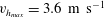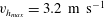We find a linear variation, demonstrating a constant velocity. Best fit of the data yields a speed $v_{h_{max}}=3.2~\text{m}~\text{s}^{-1}$ for the displacement of the maximum thickness. Interestingly, all of the data acquired at different radial positions collapse on a single master curve once the thickness and the time are normalized by their values at the maximum thickness (figure 5 b), which highlights a universal shape for the evolution of the thickness with time and radial distance. In the following, we evaluate how the thickness scales with time and radial distances, both for the short-time regime, where the thickness increases with time, and for the long-time regime, where $h$ decreases with $t$ .

Figure 5.

(a) Time evolution of the thickness of a liquid sheet. Actual and normalized data are plotted for different radial positions, as indicated in the legend of (b). Inset: Representative data on a log/log scale to highlight the two asymptotic scaling regimes. (b) Same data as those shown in (a), but normalized in the $x$ axis by the time at which the thickness is maximum, $t_{h_{max}}$ , and in the $y$ axis by the maximum thickness, $h_{max}$ . The lines correspond to the two asymptotic scaling regimes (as deduced from figure 6). Only data corresponding to the expansion regime are shown in (b). The drop diameter is $d_{0}=3.7~\text{mm}$ and the impact velocity is $u_{0}=4.0~\text{m}~\text{s}^{-1}$ . Inset: Variation of the radial position of the maximum thickness of the sheet as a function of time. The symbols are the experimental data and the line is the best linear fit of the data, yielding a velocity $r_{h_{max}}/t_{h_{max}}=3.2~\text{m}~\text{s}^{-1}$ .

3.2. Scaling and comparison with theoretical predictions

We first consider the short-time regime where $t<t_{h_{max}}$ . In this regime, the thickness varies over almost one order of magnitude, ranging from 36 to $217~{\rm\mu}\text{m}$ . We find that all data acquired at different radial positions and different times can be collapsed onto a single mastercurve if the thickness is plotted as a function of $t/r^{3}$ (figure 6 a). Moreover, a fit of the master curve (dashed line) shows that $h\propto t/r^{3}$ in this regime as predicted by Rozhkov et al. (Reference Rozhkov, Prunet-Foch and Vignes-Adler2004). More specifically, Rozhkov et al. (Reference Rozhkov, Prunet-Foch and Vignes-Adler2004) predicts

(3.1) $$\begin{eqnarray}h={\it\alpha}\,d_{0}^{3}\,u_{0}\,\frac{t}{r^{3}}\end{eqnarray}$$

with $u_{0}$ the impact velocity of the drop and $d_{0}$ the diameter of the drop. A fit of the experimental data yields ${\it\alpha}=0.061$ . This value is twice as large as the value ( ${\it\alpha}\approx 0.038$ ) derived by Rozhkov et al. (Reference Rozhkov, Prunet-Foch and Vignes-Adler2004) for roughly equivalent experimental conditions. Note that in Rozhkov et al. (Reference Rozhkov, Prunet-Foch and Vignes-Adler2004) ${\it\alpha}$ could be evaluated based on the observation of Mach–Taylor rupture waves generated by cutting radially the liquid sheet with a very thin obstacle, but not from thickness measurements. Hence, at short times, experimental data are well accounted for by the model developed by Rozhkov et al. (Reference Rozhkov, Prunet-Foch and Vignes-Adler2004). This model is predicted to be valid at short times, up to three times the typical collision time ${\it\tau}_{coll}=d_{0}/u_{0}=0.93~\text{ms}$ . Our data fall safely within this limit as, independently of the radial position, the maximum thickness occurs at times no longer than 2 ms (inset of figure 5 b). One key hypothesis of this model is that a point source, i.e. the impacting drop, feeds the sheet at a constant volume rate. We directly check this assumption thanks to side-view images of the drop impacting the target and feeding the liquid sheet (figure 7 a,b). We evaluate the time evolution of the volume of the liquid drop still available on the target, assuming that the drop remains axisymmetric at all times. The volume $V$ of the liquid is measured to decrease linearly with time yielding a constant volume rate $Q=-\text{d}V/\text{d}t=12.1~\text{ml}~\text{s}^{-1}$ , in relatively good agreement with the value ( $Q\simeq 6~\text{ml}~\text{s}^{-1}$ ) found indirectly by Rozhkov et al. (Reference Rozhkov, Prunet-Foch and Vignes-Adler2004).

Figure 6.

Same data as in figure 5 but plotted as a function of $t/r^{3}$  (a) and $1/rt$  (b) where $r$ is the radial distance and $t$ is the time elapsed from the impact of the drop. The data corresponding to $t<t_{h_{max}}$ are shown in (a), and those corresponding to $t>t_{h_{max}}$ are shown in (b). Same symbols as in figure 5. The dashed lines are power law fits of the experimental data with a slope of 1.

Figure 7.

(a,b) Side views of a liquid drop impacting a target, at time $t=0.10~\text{ms}$ (a) and $t=0.79~\text{ms}$ (b). (c) Time evolution of the volume of liquid on the target. Symbols are experimental data and the continuous line is a linear fit yielding a constant liquid ejection rate. Here, the drop diameter is $d_{0}=3.7~\text{mm}$ and the impact velocity is $u_{0}=4.0~\text{m}~\text{s}^{-1}$ .

On the other hand, in the late stage of the expansion regime, $t>t_{h_{max}}$ , the thickness varies between 26 and $191~{\rm\mu}\text{m}$ . We find that all data acquired at different radial positions can be collapsed onto a single master curve if the thickness is plotted as a function of $1/rt$ (figure 6 b). We find that $h\propto 1/rt$ , as predicted by Villermaux & Bossa (Reference Villermaux and Bossa2011). More specifically, Villermaux & Bossa (Reference Villermaux and Bossa2011) predicts

(3.2) $$\begin{eqnarray}h={\it\beta}\frac{{\rm\pi}d_{0}^{3}}{6u_{0}}\frac{1}{rt}.\end{eqnarray}$$

A fit of the experimental data provides an estimate of the prefactor ${\it\beta}=0.142$ . Note that this value is in very good agreement with the predicted value ( ${\it\beta}=(1/2{\rm\pi})=0.159$ ).

Combining our findings for the scaling with time and position of the sheet thickness for the two stages of the expansion regime, one can provide a prediction for the maximum thickness position. By equalling the two functional forms found for the thickness, (3.1) and (3.2), one finds

(3.3) $$\begin{eqnarray}v_{h_{max}}=r_{h_{max}}/t_{h_{max}}=\sqrt{\frac{6{\it\alpha}}{{\rm\pi}{\it\beta}}}\,u_{0}.\end{eqnarray}$$

First, (3.3) shows that the position of the maximum thickness moves at a constant velocity with time, as found experimentally. Moreover, it predicts that the velocity is controlled by the impact velocity $u_{0}$ . The proportionality constant between $v_{h_{max}}$ and $u_{0}$ is 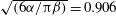$\sqrt{(6{\it\alpha}/{\rm\pi}{\it\beta})}=0.906$ . Hence, one predicts $v_{h_{max}}=3.6~\text{m}~\text{s}^{-1}$ (for $u_{0}=4.0~\text{m}~\text{s}^{-1}$ ), in good quantitative agreement with the direct measurements ( $v_{h_{max}}=3.2~\text{m}~\text{s}^{-1}$ ). The good agreement can also be inferred from the normalized experimental data shown in figure 5(b), where the lines corresponding to fits of the data in the two regimes are found to cross very close to the point corresponding to $h=h_{max}$ and $t=t_{h_{max}}$ .

3.3. Results at different Weber numbers

To check the generality of our measurements, we perform the same type of measurements and analysis as detailed above, for different Weber numbers where the impact drop velocity and the volume of the drop are varied. Five different experimental conditions, for which the Weber numbers varies between 320 and 810, are performed. In all experiments, we vary the diameter of the target to keep constant (0.6) the ratio between the diameter of the drop and that of the target. Figure 8 shows the time evolution of the diameter of the liquid sheet for the different experiments. The maximum extension of the sheet occurs at a time that depends on the drop diameter and not on the impact velocity. We find that the maximum extension occurs roughly at the same normalized time $T=0.40\pm 0.01$ . Here the standard deviation results from the statistics over the five experimental configurations. We measure that the sheet expands more as $\mathit{We}$ increases, from $d_{max}/d_{0}=4.1$ to $d_{max}/d_{0}=6.1$ . Although on a very restricted range, we find that our data are compatible with a maximum expansion scaling with $(\mathit{We})^{0.5}$ , as observed and predicted theoretically for liquid sheets expanding in air (Rozhkov et al. Reference Rozhkov, Prunet-Foch and Vignes-Adler2004; Villermaux & Bossa Reference Villermaux and Bossa2011) but also on solid surfaces (Bennett & Poulikakos Reference Bennett and Poulikakos1993; Eggers et al. Reference Eggers, Fontelos, Josserand and Zaleski2010; Marengo et al. Reference Marengo, Antonini, Roisman and Tropea2011). A fit of the data using the functional form 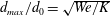$d_{max}/d_{0}=\sqrt{\mathit{We }/K}$ gives $K=19$ , in excellent agreement with the values ( $K=20$ ) given in Rozhkov et al. (Reference Rozhkov, Prunet-Foch and Vignes-Adler2004) for similar experimental conditions.

Figure 8.

Sheet diameter evolution for several experiments at different $\mathit{We}$ numbers as indicated in the legend. Inset: Maximal expansion plotted as a function of $\mathit{We}$ . Symbols are experimental data and the line is a power-law fit with an exponent of 0.5: 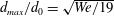$d_{max}/d_{0}=\sqrt{\mathit{We }/19}$ .

The raw data of the sheet thickness in the short-time regime and long-time regime of the expansion stage are shown in figure 9(a) as a function of $t/r^{3}$ and in figure 9(c) as a function of $1/rt$ . Overall the thickness varies between 12 and $272~{\rm\mu}\text{m}$ , and the maximal thicknesses are measured for the experiments performed with $d_{0}=4.8~\text{mm}$ and $u_{0}=2.8~\text{m}~\text{s}^{-1}$ ( $\mathit{We}=538$ ). In all cases a good scaling of the data acquired at different radial positions is obtained, showing the robustness of our findings. Using as normalized data, $H=h/d_{0}$ , $R=r/d_{0}$ , $T=t/{\it\tau}$ and $U=(u_{0}{\it\tau}/d_{0})$ , equation (3.1) for the short-time expansion regime ( $t<t_{h_{max}}$ ) can be rewritten as

(3.4) $$\begin{eqnarray}H={\it\alpha}\,\frac{UT}{R^{3}}\end{eqnarray}$$

and (3.2) for the late-time expansion regime ( $t>t_{h_{max}}$ ) can be rewritten as

(3.5) $$\begin{eqnarray}H={\it\beta}\frac{{\rm\pi}}{6}\frac{1}{URT}.\end{eqnarray}$$

Figure 9.

Evolution with time, $t$ , and radial distance, $r$ , of the thickness of a liquid sheet for five different experimental configurations as indicated in the legend: (a,b) correspond to data in the early stage expansion regime ( $t<t_{h_{max}}$ ) and (c,d) correspond to data in the late stage expansion regime ( $t>t_{h_{max}}$ ). (a,c) Actual thickness plotted as a function of (a) $t/r^{3}$ and (c) $1/rt$ . (b,d) Normalized thickness, $H$ , plotted as a function of (b) $UT/R^{3}$ , and (d) $1/URT$ . In (b,d), the dashed lines are power-law fits of the experimental data with a slope of 1.

Remarkably, figure 9(b,d) show a nice collapse of the data acquired for different Weber numbers once plotted in a normalized fashion. A fit with a power law with an exponent 1 of the data in the early expansion regime (figure 9 b) gives ${\it\alpha}=0.062$ , and a fit with a power law with an exponent 1 of the data in the late stage of the expansion regime (figure 9 d) gives ${\it\beta}=0.144$ . By equating (3.4) and (3.5), one predicts a constant normalized velocity for the maximum thickness $V_{h_{max}}=(R/T)_{h_{max}}=\sqrt{(6{\it\alpha}/{\rm\pi}{\it\beta})}U=0.91U$ . By directly measuring the normalized velocity of the thickness maximum for the different experiments, we find 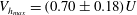$V_{h_{max}}=(0.70\pm 0.18)U$ , in good agreement with the previous determination.

3.4. Azimuthal thickness modulations

Thanks to the presence of a dye in the sheet, we are able to directly visualize small fluctuations of the thickness of the liquid sheet. We have previously integrated the values of the thickness measured at different azimuthal angles to obtain averaged data that just depend on the radial distance. A careful examination of the liquid sheet shows however a clear azimuthal modulation of the thickness. Thicker than the average, channels are observed to run over the whole extension of the sheet (figure 10 a). The profile of the thickness along a circle centred at the centre of the target clearly shows fluctuations of the thickness of typical amplitude $15~{\rm\mu}\text{m}$ (hence, approximately 30 % of the average thickness ( $52~{\rm\mu}\text{m}$ )). Moreover, the channels are rather regularly arranged as evidenced by a peak in the Fourier transform of the profile (figure 10 d), indicating a characteristic spacing of $15^{\circ }$ between adjacent channels. We are not aware of any experimental or theoretical studies of such thickness modulations. We were not able, however, to see any clear correlation between the thickness modulation and the rim corrugation. Note that the thickness modulation can also be inferred from the side view of a sheet, as shown in figure 10(b). We believe that these phenomena would deserve further investigations.

Figure 10.

Front (a) and side (b) views of liquid sheets showing a modulation of the thickness. In (a) (respectively (b)) $t=1.03~\text{ms}$ , $T=0.064$ (respectively $t=1.44~\text{ms}$ , $T=0.09$ ). (c) Azimuthal profile of the thickness along the circle shown in (a). (d) Fourier transform of the profile shown in (c). Here, the drop diameter is $d_{0}=3.7~\text{mm}$ and the impact velocity is $u_{0}=4.0~\text{m}~\text{s}^{-1}$ .