


1. Introduction
Supersonic transport aircraft (SST) are typically designed to cruise at specific altitudes and speeds to maximize the propulsive and aerodynamic efficiency of the vehicle. However, a large part of the operating life of SST and supersonic fighters is spent at lower speeds in the transonic regimes, where flutter margins are at a minimum (Dowell Reference Dowell2015). Rarely, however, are the types of instabilities encountered during the transonic flight fully predicted by numerical simulations and analytical models, resulting in costly flights for aircraft certifications. In-flight documentation in the public domain has revealed that dynamic instability is typically exhibited as an asymmetric oscillatory motion of the wings (Denegri Reference Denegri2000). The amplitude of the limit-cycle oscillations (LCOs) does not normally exceed the structural limits but can lead to fatigue and vibrations that can substantially reduce the operational flight envelop.
The F-16 is probably one of the most famous and documented examples of in-flight structural aeroelastic instabilities (Foughner & Besinger Reference Foughner and Besinger1977; Denegri Reference Denegri2000; Dowell Reference Dowell2015; Chen et al. Reference Chen, Zhang, Zhou, Wang and Mignolet2018). Designed to carry up to approximately 10 tons of weapons, sensors and external fuel tanks, the F-16 experienced LCOs during flight tests. Extensive ground testing demonstrated that the presence of external stores under the wings significantly promoted the occurrence of flutter. It was also found that fuel consumption from the external stores had to follow a specific procedure to avoid the onset of dynamic instabilities (Foughner & Besinger Reference Foughner and Besinger1977). However, linear models typically failed in predicting the critical Mach number and the amplitude of LCOs.
Transonic fluid–structure interactions (FSIs) are strongly nonlinear, because the response of the structure is not always proportional to the external aerodynamic load. Normal shock-wave/boundary-layer interactions on the wing profile can lead to a substantial increase in wave drag (Babinsky & Ogawa Reference Babinsky and Ogawa2008) and it is often considered one of the main sources of nonlinearity (Dowell Reference Dowell2015). The normal shock promotes boundary-layer separation and the formation of a detached shear layer. The latter can affect the shock position, thus changing the conditions upstream. This feedback loop results in self-excited shock-induced oscillations which can lead to a large variety of structural dynamic instabilities such as control surface buzz and buffeting (Edwards Reference Edwards1996). Recent studies have demonstrated that buffeting can be mitigated by placing vortex generators near the leading edge of the wing and by using trailing-edge deflectors (Caruana et al. Reference Caruana, Mignosi, Corrège, Le Pourhiet and Rodde2005). Other studies have focused on wing morphing and shape optimization (Babinsky & Ogawa Reference Babinsky and Ogawa2008; Wengang et al. Reference Wengang, Chuanqiang, Yiming and Weiwei2020). These techniques aim at reducing shock strength by smearing the normal shock into a  $\lambda$-shock thus delaying shock-induced separation and abating shock-induced oscillations.
This scenario is further complicated by the presence of structural sources of nonlinearity. An example is control surface free play, that has reportedly induced LCOs in a number of flights (Whitmer et al. Reference Whitmer, Christopher, Kelkar, Vogel, Chaussee, Ford and Vaidya2012; Dowell Reference Dowell2015). Military aircraft typically employ all-movable tails instead of the stabilizer–elevator combination, thus it becomes important to assess the rigidity of the actuation system to avoid the occurrence of flutter also for otherwise stable configurations (Hoffmann & Spielberg Reference Hoffmann and Spielberg1954). Free play is a phenomenon analogous to the backlash in gears, with the all-movable wing (or the flap) free to oscillate at trim by a limited deflection angle. While this research area is very active, it is also affected by a substantial lack of experimental data. It is enough to consider that the current US military specifications for free play date back to subsonic wind-tunnel tests conducted in the 1950s (Hoffmann & Spielberg Reference Hoffmann and Spielberg1954; Whitmer et al. Reference Whitmer, Christopher, Kelkar, Vogel, Chaussee, Ford and Vaidya2012). The bending of wings can also be an important source of nonlinearity. Low-aspect-ratio wings, typical of SST such as the Concorde, can behave as structural plates and thus undergo a form of instability very similar to panel flutter (Dowell Reference Dowell2015). In the presence of lateral bending, skin panels can be subjected to membrane stress, which results in a localized stiffening of the wing (Dowell Reference Dowell2015), thus highlighting the limitations of linear models for flutter predictions.
The type of flutter can vary as a consequence of small changes in upstream parameters. A numerical study on rigid airfoils with two degrees of freedom from Edwards et al. (Reference Edwards, Whitlow, Bennett and Seidelt1983) shows that flutter speed can change by more than 50 % with a change in angle of attack of only 1.5 $^\circ$; in the lower flutter boundary, the instability type is similar to a single degree of freedom (or shock-induced) flutter, while coalescence of plunge and pitch modes characterize the flutter's upper boundary. Concerning boundary-layer transition, it appears that the exact location of the transition point does not play a key role; Gordnier & Melville (Reference Gordnier and Melville2000) numerically showed that, if instead of assuming a fully turbulent boundary layer the transition point is artificially shifted at 30 % of the chord, the critical dynamic pressure increased by only approximately 3 %. However, contradictory findings were discovered by a quasi-three-dimensional numerical study on compressor blades undergoing transonic stall flutter (Isomura & Giles Reference Isomura and Giles1998); in this instance, the location of transition was determined using the $e^n$ method and proved to introduce localized changes to the pressure distribution by approximately a factor ten. The question thus arises as to whether the role of boundary-layer transition is enhanced in three-dimensional problems.
From a numerical point of view, transonic FSI is computationally expensive, and often more demanding than supersonic or even hypersonic FSI when thermal effects are neglected. One of the main problems is that the flow is practically always three-dimensional because disturbances travel in every direction and the separation bubble (if present) has an irregular shape, often spilling at the wing tip. Conversely, supersonic aerodynamic models such as piston theory (Ashley & Zartarian Reference Ashley and Zartarian1956) are point functions that can accurately predict pressure variations based only on local and free-stream flow properties, a phenomenon often referred to as zero-memory effect (Dowell Reference Dowell2015). When wind-tunnel experiments are modelled, special attention has to be paid to test-section wall interactions. Except for the case of panel flutter, where displacements are in absolute terms typically small, this problem often necessitates a full test-section model, thus further increasing the computational cost. In this scenario, reduced-order models can play a role. Solving the linearized potential equation for small perturbation has often been considered the main way to tackle transonic FSI (Dowell Reference Dowell2022), clearly posing a limit in terms of maximum deflection. In this regard, it is important to note that large deflection does not necessarily translate in a promotion of instabilities. Consequently, knowledge on the actual behaviour of wings for large strains is simply insufficient because of large wall interference effects in transonic wind tunnels, danger to human lives during flight tests and the inaccuracy of the linearized potential theory employed in numerical simulations. Time domain integration is often preferred to the frequency expansion method, because the latter employs a modal superposition of harmonic loads (Edwards et al. Reference Edwards, Whitlow, Bennett and Seidelt1983). Thus the frequency-based approach will only work for small shock oscillations around the static steady position. Conversely, time integration methods also allow for the shock to disappear for small deflections, thus are most suitable to solve the intrinsic nonlinear character of transonic FSI (Borland & Rizzetta Reference Borland and Rizzetta1981).
A modern approach is to enrich the aerodynamic models using steady-state solutions, which can be considered computationally inexpensive both under a mesh-development and solve-time point of view. The steady-state solution can be used as a baseline solution, which can be calculated also for large deflections. Thus the linearized potential theory can be used to calculate the small-perturbation solution, which is based on a priori steady computations. This approach was applied by Opgenoord, Drela & Willcox (Reference Opgenoord, Drela and Willcox2018) to a two degrees-of-freedom airfoil. In this work, the temporal variation in circulation was used to calculate lift and pitching moment evolution. For large-aspect-ratio wings, two-dimensional results can be utilized to approximate the aerodynamic pressure distribution as long as the effective speed direction parallel to the airfoil section is corrected with the effective back-sweep angle (Barmby, Cunningham & Garrick Reference Barmby, Cunningham and Garrick1950). This approach is generally referred to as strip theory, which assumes that every section of the wing is aerodynamically independent of the adjacent ones. Close to the critical Mach number and for large aspect ratios, this approach can lead to reasonably good results with errors smaller than 5 % to 10 % (Opgenoord, Drela & Willcox Reference Opgenoord, Drela and Willcox2019). However, large separation regions and strong tip vortices can invalidate the theory, thus resulting in large errors.
Stall flutter is another example of a very nonlinear type of structural instability that is difficult to solve numerically. Unfortunately, theoretical models are useful only towards isolating a few of the main driving phenomena behind stall flutter (Sisto Reference Sisto2022). Generally, stall flutter is not caused by the classical mode-merging mechanism. The near-stall nonlinear aerodynamic response is the main cause of instability rather than elastic coupling between the first two modes. For a single degree-of-freedom rigid airfoil, Sisto (Reference Sisto1953) showed that the type of flutter presents a dependence on the lag in the aerodynamic response and the location of the elastic axis. However, the analytical model quickly becomes too complex for interpretation, whilst assuming periodic motion, small perturbations, two-dimensional (2-D) flow, a single degree of freedom and ignoring hysteretic behaviour. Vortex method is a powerful alternative, however, it is limited to 2-D incompressible problems and it requires a condition for boundary-layer separation (Sisto, Wu & Jonnavithula Reference Sisto, Wu and Jonnavithula1953). Transonic stall flutter has received special attention mainly (and almost solely) in the context of turbomachinery, particularly the first compressor stages where the hub-to-tip ratios are typically below 0.4 (Saravanamuttoo, Rogers & Cohen Reference Saravanamuttoo, Rogers and Cohen2001). The reason is that experiments are expensive and typically require a blade cascade type of experimental set-up. The first problem is probably to establish if blade stall is the main cause of flutter. Typically, the torsional mode is considered the main driving phenomenon behind stall flutter, thus resulting in a one degree-of-freedom type of instability. However, compressor blades bending can result in a geometrical change of the blade passage, thus bending flutter could be more important than torsion stall flutter (Isomura & Giles Reference Isomura and Giles1998). For this reason, the type of instability could generally be hybrid, thus nonlinear in two degrees of freedom, and there could be a large degree of coupling. In a quasi-3-D numerical study, Isomura & Giles (Reference Isomura and Giles1998) showed that compressor blade flutter was purely induced by shock oscillations; a minimal bending motion of the blades resulted in the shock moving in the passage between the started and un-started position. In this context, it is necessary to perform and simulate a fundamental experiment that is repeatable and that presents large deflection, separation, stall and associated non-negligible 3-D effects.
The present work is a numerical and experimental study of thin rectangular plates undergoing FSIs at Mach 0.8 for a range of angle of attack between 0 $^\circ$ and $4^\circ$; the objective is to develop a computational fluid dynamics (CFD)-based aerodynamic pressure model that can be used to calculate the pressure distribution on low-aspect-ratio elastic wings undergoing large deformations, with special attention to stall-flutter margin predictions. In § 2, details of the facility, wind-tunnel model and experimental technique are provided. Sections 3 and 4 are devoted to the description of the numerical technique adopted in fully coupled FSI simulations and related results. Section 5 concerns the implementation of low-fidelity aerodynamic models and the assessment of their accuracy relative to high-fidelity FSI simulations. Section 6 offers a comparison between simulations and experiment. Conclusions are drawn in § 7.
2. Experimental set-up
2.1. The National Cheng Kung University transonic wind tunnel
The experiments shown herein were performed in a transonic wind tunnel (see figure 1) located at the Aerospace Science and Technology Research Center (ASTRC) of the National Cheng Kung University (NCKU). This facility provides a flow with variable Mach number between  $M_\infty = 0.2$ and $M_\infty = 1.4$ and Reynolds number of $Re \sim 20\times 10^6$ m $^{-1}$. The total pressure is monitored upstream of the stilling chamber using a rotary shut-off ball valve and a rotary perforated sleeve stagnation-pressure control valve. The total pressure is approximately 50 psia ( ${\sim }345$ kPa), while three high-pressure reservoirs are at a pressure of 5.15 MPa at room conditions. Temperature is controlled using a thermal mass matrix which allows for a maximum drop smaller than 10 K during 30 seconds of test time. The dew point is kept at 230 K. The test section has a square frontal area, with 600 mm long edges, and it has a length of 1.5 m. A typical test duration is of the order of 10 to 30 seconds at Mach 1. Referring to figure 1(b), the nominal free-stream conditions employed in this work are $M=0.77$, $p_\infty = 116\,196$ Pa, $Re_\infty = 22.33 \times 10^6$ m $^{-1}$. Figure 1(c) shows some of the wind-tunnel calibration studies regarding flow angularity at steady conditions (Chung, Miau & Yieh Reference Chung, Miau and Yieh1994, Reference Chung, Miau and Yieh1995). The flow incidence was derived from the difference in pressure measured on a five-cone-probe rake. The results indicated a variation smaller than $0.1^{\circ }$ for all values of the Mach number between 0.3 and 1 at steady conditions.

Figure 1. Transonic wind tunnel at the Aerospace Science and Technology Research Center of NCKU (1 – isolation valve, 2 –  $p_0$ housing valve, 3 – pressure pipe, 4 – stilling chamber, 5 – nozzle, 6 – test section, 7 – resistor flow Section, 8 – leak expansion section). (a) Schematics of the facility. (b) Free-stream characteristic. (c) Angularity measurements from Chung et al. (Reference Chung, Miau and Yieh1995).
2.2. Wind-tunnel model and material
As shown in figure 2, the experiment involved a 200 mm long and 100 mm wide cantilevered metal plate, with a thickness of 2 mm. The initial numerical and analytical study concerned aluminium alloy material with nominal properties and infinitely elastic. This permits a large range of deformation, which makes it possible to test the limits of the modelling capabilities. However, experimental data presented herein are those of titanium alloy (Ti-6Al-4 V). The initial transient, characterizing the facility start-up phase, involves large aerodynamic loads and a rapidly changing flow angularity, often resulting in structural failure. Titanium alloy is used because its yield stress is typically four times as large as aluminium or steel, thus it allows the model to survive the initial pressure transient. The mechanical properties shown in table 1 are derived through free vibration tests. The bending stiffness is assessed by matching the first two natural frequencies with those calculated through a finite-element model (FEM). The damping ratio is here defined as  $\zeta = {\rm \Delta} f/f_1$, where $f_1$ is the fundamental frequency and ${\rm \Delta} f$ is the half-width of $f_1$. As shown in figure 2(a), the panel is clamped using two ‘L’ shape elements in order to avoid residual panel displacement near the root. The clamped panel is then attached to a flange that is framed to the wall support (figure 2b,c). The flange can rotate so as to modify the angle of attack; the latter can be measured with a precision lower than $0.05^{\circ }$ using a laser displacemeter. As explained in the previous section, it is important to reduce blockage to below 1 %–2 % not only in the static state but also when the panel is deforming, which exposes more frontal area to the incoming flow. As shown in figure 2(d), the problem is circumvented by removing a window and clamping the model to the sidewall.

Figure 2. Wind-tunnel model technical drawings: (a–c) details of the clamping method and (d) positioning within the test section.
Table 1. Test panel properties (the Poisson ratio  $\nu$ is an assumed property in all cases).

2.3. Measurements
All the quantitative measurements are conducted using high-speed visualization at a sampling rate no greater than 2 kHz to increase the signal-to-noise ratio. High-speed camera images, such as those shown in figure 3, are used to track both plate tip inclination and vertical displacement. During the experiment the tip of the plate is painted with a reflective paint; consequently, it is possible to track the tip vertical position with an accuracy of 0.25 mm during the post-processing analysis (pixel resolution is 0.12 mm).

Figure 3. Example of image post-processing (flow from right). Contour variable is pixel light intensity. (a) Wind off. (b) Wind on.
Originally, displacement measurements were supposed to be performed using a laser displacemeter ( $\mu -\epsilon$ optoNCDT ILD 1420-200) with a measuring range of 100 mm, a repeatability below 10 $\mathrm {\mu }$m and a sampling rate of 4 kHz. In these initial tests, the laser sensor was located on the floor of the test section, as shown in figure 4(a). Even if the total frontal area occupied was less than 1 % of the test-section frontal area, the sensor support always induced a positive angle of attack of approximately half a degree – in some cases inducing structural failure. Thus the laser sensor here is only used to assess the accuracy of the displacement data from the image post-processing. As shown in figure 4(b), laser- and camera-based measurements almost overlap, with the majority of the small disagreement due to a lower camera frame rate.

Figure 4. (a) Wind-tunnel model and laser sensor in the test section and (b) comparison between laser- and camera-based measurements.
3. Numerical method
The FSI numerical simulations were computed by coupling the fluid solver with the structural solver at every time step  ${\rm \Delta} t = 0.1$ ms. The commercial software ANSYS/Fluent was used to solve the 3-D transient Navier–Stokes equations, which can be expressed as follows:
 $$\begin{gather} \frac{\partial \rho}{\partial t}+\frac{\partial(\rho u_j)}{\partial x_j}=0, \end{gather}$$
 $$\begin{gather}\frac{\partial(\rho u_i)}{\partial t} + \frac{\partial(\rho u_i u_j)}{\partial x_j}={-}\frac{\partial p}{\partial x_i} + \frac{\partial \hat{\tau}_{ji}}{\partial x_j}, \end{gather}$$
 $$\begin{gather}\frac{\partial(\rho E)}{\partial t} + \frac{\partial(\rho u_j H)}{\partial x_j}=\frac{\partial}{\partial x_j}\left(u_i \hat{\tau}_{ij} + (\mu+\sigma^*\mu_T)\frac{\partial k}{\partial x_j}-q_j\right), \end{gather}$$
where  $\mu$ is the molecular viscosity and $\hat {\tau }_{ij}$ is the total viscous shear stress tensor
 \begin{equation} \hat{\tau}_{ij}=(\mu+\mu_T)\left(\frac{\partial u_i}{\partial x_j}+ \frac{\partial u_j}{\partial x_i}-\frac{2}{3}\frac{\partial u_k}{\partial x_k}\delta_{ij}\right)- \frac{2}{3}\rho k\delta_{ij}, \end{equation}
where  $E=(C_v T+u_i u_i/2 +k)$ and $H=(C_p T+u_i u_i/2 +k)$ are the mean total specific energy and enthalpy, respectively; the heat flux vector can be written as
 \begin{equation} q_j={-}\left(\frac{\mu}{Pr_L}+\frac{\mu_T}{Pr_T}\right)\frac{\partial C_pT}{\partial x_j}, \end{equation}
where  $Pr$ is the Prandtl number. Adiabatic wall condition is assumed, thus wall heat-flux $q_w = 0$. The equations are coupled with the ideal gas equation for air. Additionally, the ${k-\omega}$ shear-stress transport (Menter Reference Menter1994) equations are used to calculate the eddy viscosity term $\mu _T$. This turbulence model was chosen because of its good performance in boundary layers as well as in free shear layers. The transport equations of specific turbulence kinetic energy $k$ and dissipation rate $\omega$ can be written as follows:
 $$\begin{gather} \frac{\partial (\rho k)}{\partial t} + \frac{\partial(\rho u_j k)}{\partial x_j}=P_k(\beta^*\rho\omega k)+ \frac{\partial}{\partial x_j}\left[(\mu+\sigma_k\mu_T)\frac{\partial k}{\partial x_j} \right] \end{gather}$$
 $$\begin{gather}\frac{\partial (\rho \omega)}{\partial t} + \frac{\partial(\rho u_j \omega)}{\partial x_j}=P_k(\beta\rho\omega^2)+\frac{\partial}{\partial x_j}\left[(\mu+\sigma_\omega\mu_T)\frac{\partial \omega}{\partial x_j}\right]+2\rho(1-F_1)\sigma_{\omega_2}\frac{1}{\omega}\frac{\partial k}{\partial x_j}\frac{\partial \omega}{\partial x_j}, \end{gather}$$
where  $\alpha$, $\alpha ^*$ and $\beta$ are functions of the turbulence Reynolds number $Re_T=\rho k/\omega \mu$ (Wilcox Reference Wilcox1994); consequently, $\mu _T$ can be expressed as $\mu _T =\alpha ^* Re_T \mu$. Here, $P_k$ and $P_\omega$ are the net production per unit dissipation for $k$ and $\omega$ (Wilcox Reference Wilcox1994) and $F_1$ is the blending function between the standard $k-\omega$ model ( $F_1 \rightarrow 1$, near the wall) and the $k-\epsilon$ model ( $F_1 \rightarrow 0$). These equations were numerically solved with an implicit, cell-centred, second-order upwind solver.
Details of the discretized domain are given in in figure 5. Two types of mesh are considered; the simplest, shown in figure 5, is a reduced domain ( $350\,{\rm mm} \times 350\,{\rm mm}\times 400\,{\rm mm}$) with 0.6 million cells. This value was decided based on mesh independence studies, which are summarized in figure 6(a). In terms of boundary conditions, the plane adjacent to the plate is set to a viscous wall, while the other five enclosing planes are non-reflective boundaries. In § 6, the numerical domain includes the whole test section in order to simulate the experiments with enhanced accuracy. In this case, the mesh domain is larger ( $600\,{\rm mm}\times 600\,{\rm mm}\times 1200\,{\rm mm}$) with a cell count of 2 million cells. Both the meshes present the same level of refinement near the plate, with a minimum length and height of 2 and 0.1 mm respectively. The maximum $Y^+$ at the wall is smaller than 0.01. During the coupling, nodal displacements are retrieved from the FEM solver and applied to the mesh. Smoothing techniques were employed to maintain the mesh density of the boundary-layer region relatively unaffected, while diffusing all the residual mesh deformation away from the wall.

Figure 5. Structured mesh details. The mesh is retrieved from the simulations, in this case the mesh is deformed due to the FSI.

Figure 6. Mesh independence study for (a) fluid domain, (b) plate and (c) time independence study (for nominal titanium alloy properties,  $\alpha = 4^\circ$).
The structure is a rectangular plate with a chord of 100 mm and a span of 200 mm, with a converged cell size of 2.5 mm (see figure 6b). The maximum thickness employed was 2.2 mm, thus a shell element type was employed. This choice permitted to change the wing thickness without remeshing the fluid domain. The shell element is a 3-D 8-node membrane with six nodal degrees of freedom. The materials considered are linearly elastic and isotropic. Referring to the governing equation in the finite-element model formulation
 \begin{equation} [M]\ddot{w}+[C]\dot{w}+[K]w=f, \end{equation}
where  $w$ is the nodal displacement vector, $f$ represents nodal loading while $M$,
$M$,  $C$,
$C$,  $K$ are mass, damping and stiffness matrices, respectively. The Rayleigh damping model (Liu & Gorman Reference Liu and Gorman1995) was employed to calculate $C=\alpha M + \beta K$ based on the first two natural circular frequencies as follows:
 \begin{equation} \alpha=\frac{2\omega_1\omega_2}{\omega_2+\omega_1}\zeta, \quad \beta=\frac{2}{\omega_2+\omega_1}\zeta, \end{equation}
where  $\zeta$ is the damping ratio. The coupling time step ${\rm \Delta} t = 0.1$ ms is set equal to the marching time step of the fluid and structure solver. The time independence study is shown in figure 6(c).
It is possible to perform a preliminary estimate of the accuracy of FSI simulations. Based on the mesh and time independence study, the error induced by poor refinement and a coarse time step should be smaller than 0.1 N in terms of lift. Additional simulations were performed to evaluate the error induced by the zero-thickness approximation in the CFD solver. Neglecting the actual thickness of the plate (2 mm) will induce an error of approximately 5 % in the lift production with a maximum of 8 % for large angles of attack. Drag is under-predicted by an approximately constant value smaller than 20 N.
4. High-fidelity simulations: preliminary discussion
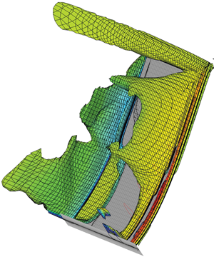
An overall qualitative description of the physics involved is shown in figure 7. The material used in this analysis is aluminium, and the plate thickness is 2 mm (see table 1). Mach 0.77 is slightly above the critical Mach number; the flow experiences a local acceleration around the leading edge, resulting in a localized supersonic area. As in the incompressible regime, the plate undergoes leading-edge stall; the latter happens less abruptly with respect to classic trailing-edge stall, and the flow generally reattaches before the mid-chord. The flow induces panel twist, which results in a larger separated region on the suction side, consequently decreasing the aerodynamic torque as well as lift and panel twist. This interplay between structure and flow induces oscillations.

Figure 7. Pressure distribution on the panel corresponding to the maximum twist and bending.
In figure 8 the solution from the high-fidelity simulation is analysed in terms of frequency response. Figure 8(a) shows the tip-displacement power spectrum for three values of angle of attack. The first peak coincides with the first natural mode (  $f_1 \equiv f_{N1}$); the second peak becomes dominant for $AOA>2^\circ$ and tends to approach the second natural frequency $f_{N2}$. A third peak is only visible for $AOA = 3^{\circ }$, however, it can be demonstrated that this is not the third mode. In figure 8(b), where the power spectrum of the surface-averaged pressure differential over the panel is shown, the largest peak at around 150 Hz always coincides with the second peak in figure 8(a) for all the angles of attack explored. This suggests that the torsional mode plays the most important role in the plate dynamics, while the bending motion appears not to significantly affect the pressure distribution. The first and second peaks in figure 8(a) have the same order of magnitude. The first peak, however, is apparent in figure 8(a) but not in figure 8(b). To this end, it is important to note that that, in figure 8(b), power fluctuations below 0.1 or 0.2 Pa $^2$ kHz $^{-1}$ cannot directly be linked to a specific structural mode. Only the second peak is clearly a consequence of the torsional mode. Conversely, generally every natural mode and associated harmonics contribute to the rise of low power fluctuations. For the case $\alpha = 3^\circ$, additional peaks are located at frequencies that are a multiple of $f_2 = 150$ Hz (i.e. $f_3 =300$ Hz, $f_4=450$ Hz,…), thus they are a consequence of the second – or torsional – mode. The latter determines periodic pressure variations with a frequency $f_2\sim f_{N2}$; however, for large values of the angle of attack (i.e. for large variations in separation-bubble size) pressure frequency breaks down into harmonics. The third structural peak in figure 8(a) is thus induced by the first of these harmonics, and it is not induced by the third structural mode of deformation. The presence of harmonics in the fluid response is not surprising, and it was observed even at higher speeds in the presence of large separated regions (Currao et al. Reference Currao, McQuellin, Neely, Gai, O'Byrne, Zander, Buttsworth, McNamara and Jahn2021). As will be discussed later, the bubble size is not a linear function of the plate twist. Consequently, even assuming a perfectly sinusoidal variation in twist, the bubble size response cannot be expressed as a simple sine function but, most generally, as a Fourier sine series which is a sum of harmonics.

Figure 8. Power spectrum as a function of angle of attack calculated from the high-fidelity 2-way solutions from the structure (a) and fluid sides (b). (a) Tip displacement (b) Mean pressure differential.
In figure 9(a) the second dominant frequencies from the tip displacement and pressure evolution are plotted against angle of attack  $\alpha$. The lock-in or coalescence between structural and fluid frequencies take place for $\alpha = 2^\circ$ with flutter occurring at $2.1^\circ$. A further coalescence point is also present at $\alpha = 0^\circ$, which, however, does not lead to flutter in the simulations. Figure 9(b) shows the LCO amplitude as well as the standard deviation of tip twist angle during 0.3 seconds of flow. The panel maximum twist can very well be interpreted as the amplitude of the second mode, which reaches LCO only for $\alpha > 2^\circ$.

Figure 9. Second-mode frequency and amplitude: (a) second frequency peak from tip displacement and pressure; (b) LCO amplitude and standard deviation of plate twist.
5. Low-fidelity aerodynamic model
The basis for this low-fidelity model is that 3-D steady-state laminar and Reynolds-averaged Navier–Stokes (RANS) simulations can be generally considered as numerically inexpensive. Every university has access to a high-power computing environment and many simulations of this kind can be run at the same time, with accurate solutions typically available within the day. While this is not generally true for transient FSI simulations, it is, however, possible to exploit these advantages, and to develop a more exhaustive low-fidelity model based on a pre-computed steady (or pseudo-transient) aerodynamics. This allows for faster FSI simulations and parametric studies for similar geometries and free-stream conditions.
In this section, 1-way FSI calculations will refer to a single exchange from the fluid solver (CFD) to the structure solver (FEM) in terms of aerodynamic load (i.e. nodal forces). During a 2-way FSI simulation, the structure solver has typically to wait in stand-by for the fluid solver to transmit the aerodynamic load. Then, the fluid solver is put on stand-by and the structural solver computes the mesh nodal displacements to be transmitted back to the fluid solver. This section is focused on the development of an aerodynamic model that can substitute the fluid solver, thus saving computational time. All the results shown in this section, except when clearly stated, are obtained for nominal aluminium properties (2 mm thick) ignoring plasticity (see table 1).
5.1. Basic formulation
The first step consists of isolating the most energetic fundamental modes contributing to the panel dynamics. For cantilevered wing geometries with high aspect ratio, variations in the pressure distribution mainly depend on the torsional mode. This is also intuitive, because without panel torsion there is no change in lift. The strip theory for example relies on the effective angle of attack of a local twisted section to compute the aerodynamic pressure. Works on cantilevered wings typically employ the strip theory in conjunction with tip loss corrections (Afonso et al. Reference Afonso, Oliveira, Vale, Lau and Suleman2017; Riso & Cesnik Reference Riso and Cesnik2023). As will be discussed, the first mode should also be considered in the presence of large bending because this might affect the local effective angle of attack. For low-aspect-ratio wings, large bending can potentially affect the pressure distribution at the root. For additional accuracy, other modes can also be considered, but higher frequency modes are generally characterized by a lower oscillation amplitude. In this section it will be proved that only two modes are strictly necessary. Displacement  $y_{MAX}$ and the maximum twist angle (at the tip of the panel) $\theta _{MAX}$ are regarded as the magnitudes of first and second mode, respectively, as defined in figure 10.

Figure 10. Schematics of the first two natural modes, namely (a) bending and (b) torsion, and quantification of their amplitude in terms of tip displacement and twist, respectively. (a) First (bending) mode. (b) Second (torsional) mode.
Considering only the second mode for the moment, a steady-state static simulation can be conducted for each amplitude value. For a range of  $\theta _{MAX}$ values, a deformed panel geometry can be generated with the shape of the second mode. Thus, a static steady-state simulation is conducted and the pressure distribution on the panel is calculated. For each value of twist a pressure-differential distribution is assigned, which is merely the difference between the pressures on the top and bottom of the plate at each location along the chord (or $x$-direction) and the span (or $z$-direction). This procedure can be repeated for different angles of attack, thus the pressure differential is now ${\rm d} p = {\rm d} p (x,z;\theta _{MAX}, \alpha )$.
Figure 11 shows the pressure differential across the panel assuming a second-mode shape. Pressure differential is the largest close to the leading edge, and it decreases along the span due to a gradual equalization between the two sides of the plate. Increments in both twist angle and angle of attack have the effect of increasing pressure and the size of the separated region.

Figure 11. Pressure-differential distribution ( ${\rm \Delta} p/ q_\infty$) as a function of angle of attack (rows) and twist $\theta _{MAX}$ (columns). The red line confines the separation region; (a,e,i) 2.4 $^\circ$, (b,f,j) 4.6 $^\circ$, (c,g,k) 6.8 $^\circ$, (d,h,l) 9 $^\circ$.
A schematic of a 1-way FSI simulation is given in figure 12. It is called 1-way because the aerodynamic load does not change with the deformation, or it is not updated. The pressure-differential distribution, calculated for a plate with a second-mode shape and a twist of  $\theta _{MAX}$, is used as the external load for a steady FEM simulation. Results are shown in figure 13(a), where on the x-axis is shown the twist corresponding to the second-mode amplitude while the resulting twist of the deformed panel is given on the y-axis. The values of $\theta _{MAX}$ lying on the line $y=x$ correspond to steady 2-way FSI solutions, because twist of the panel corresponds to the second-mode shape twist used to generate the aerodynamic load; this is analogous to a simulation where the aerodynamic load is an instantaneous function of $\theta _{MAX}$. Again, as deduced from the pressure distribution shown in figure 11, an increase in angle of attack $\alpha$ has an effect analogous to $\theta _{MAX}$, it will generally determine larger pressure-differential values and consequently larger structural deformations. In figure 13(b) the resulting twist is plotted against the second-mode twist augmented by $3\alpha /2$, thus proving that, also in a highly compressible regime, wing twist is equivalent to a linear increase in angle of attack. For larger values of angle of attack, the effect of separation offsets the overall pressure increase needed to increase twist, thus $\theta _{MAX}$ plateaus for $\alpha >3^\circ$. Additionally, since the large-deflection model is activated, larger twist angles results in an overall stiffer plate, thus further counteracting the aerodynamic torque.

Figure 12. One-way FSI simulation schematics.

Figure 13. One-way FSI simulation results. Here,  $\theta ^{\prime\prime}_{MAX}$ refers to the amplitude of the second mode used to generate the pressure distribution, $\theta _{MAX}$ is the resulting twist in the FEM solver and $\alpha$ is the angle of attack. The square symbols in both (a,b) represent the 2-way FSI solution.
As shown in figure 14, the same results can be expressed in terms of tip vertical displacement  $y_{MAX}$, i.e. amplitude of the first mode. Figure 14(a) shows that, close to $\alpha = 3^\circ$, the pressure distribution does not contribute to twist anymore, and the only effect of increasing the angles of attack is promoting bending. Figure 14(b) shows that also $y_{MAX}$ can be expressed as a monotonic function of angle of attack and twist because, except for the extreme case of a $90^\circ$ bending, an increase in pressure differential will always affect plate bending even in the presence of a large separation region.

Figure 14. One-way FSI simulation results. Here,  $\theta ^{\prime\prime}_{MAX}$ refers to the amplitude of the second mode used to generate the pressure distribution, $\theta _{MAX}$ is the resulting twist in the FEM solver and $\alpha$ is the angle of attack. The square symbols represent the 2-way steady FSI solution.
In order to perform a transient 2-way FSI simulation, the aerodynamic load has to be updated at every time step, retrieving the instantaneous values of panel twist and effective angle of attack. Figure 15 shows the procedure adopted to calculate the panel twist at every time step. It is then necessary to calculate the effective angle of attack. However, since every point on the panel will move with a different velocity, in general the effective angle of attack  $\alpha _{eff}$ will be a function of both $x$ and $z$.
$z$.

Figure 15. Procedure for the calculation of tip twist  $\theta _{MAX}$ knowing the leading- and trailing-edge node positions.
Figure 16 shows the procedure to calculate the local vertical speed at every time step at the tip of the plate. Assuming small elevation  $y_{max}(t)$ (thus the amplitude of the bending mode is small) the local effective angle will depend on the vertical local speed and the rotational velocity of the edge. These values can be computed at each time step knowing, $y_{LE}$, $y_{TE}$ and $y_{MC}$ as follows:
 \begin{equation} v_{MC}(t+{\rm \Delta} t)=\frac{y_{MC}(t+{\rm \Delta} t)-y_{MC}(t)}{{\rm \Delta} t},\quad \omega(t)=\frac{\theta_{MAX}(t+{\rm \Delta} t)-\theta_{MAX}(t)}{{\rm \Delta} t}, \end{equation}
where  ${\rm \Delta} t$ is the time step. The vertical velocity at every point along the plate can be approximated assuming a parabolic trend, that is:
 \begin{equation} v(x,z)=v(x,L) \left(\frac{z}{L}\right)^2. \end{equation}
Figure 16. Procedure for the calculation of the local effective angle  $\alpha _{eff}$ at the tip.
A parabolic trend is chosen because it resembles the first-mode shape and the first derivative is zero at the root. For large bending ( $\kern0.7pt y_{MAX}>0.4 L$), the vertical velocity $v_{MC}$ should be substituted with the local normal velocity, as explained in figure 17. The normal velocity is the sum of the projection of vertical and horizontal velocities on the local unit normal vector. Using the normal velocity is more accurate, but calculating the face normal of every element at every time step might slow down the calculations if do-loops are employed.

Figure 17. Definition of the normal velocity at the tip of the plate.
In order to calculate the local pressure
 \begin{equation} p(x,z)=p(\theta_{MAX},\alpha_{eff}(x,z); x,z), \end{equation}
it is then necessary to interpolate pressure for a twist angle  $\theta _{MAX}$ and an angle of attack $\alpha _{eff}(x,z)$ at every time step. If only two parameters are needed to calculate the pressure distribution, this is easily accomplished by linearly interpolating the values of pressure between those previously calculated for a sufficiently large range of twist angle and angle of attack, as shown in figure 11. Figure 18 shows a comparison between 1-way and 2-way simulations, for different values of angle of attack. It is important to notice that, during the simulation, the effective angle of attack $\alpha _{eff}$ can be significantly larger than the geometrical angle of attack $\alpha$, thus steady simulations have to be calculated a priori for a sufficiently large range of $\alpha$ values. However, if more parameters are needed – as in the case where it is necessary to also consider the contribution of the first mode to the pressure distribution – this process can become more cumbersome, as a very large number of steady-state simulations have to be conducted a priori to make the interpolation possible. Fewer simulation data points can be employed using kriging method, resulting, however, in longer computational times.

Figure 18. Comparison between 1-way, 2-way steady and 2-way transient simulations for different values of angle of attack: (a)  $\alpha = 1^\circ$, (b) $\alpha = 2^\circ$, (c) $\alpha = 3^\circ$.
Based on the correlation shown in figure 14, it is possible to express the local pressure as a function of only one parameter
 \begin{equation} p(x,z) = p(\theta_{eff}; x,z), \end{equation}
with
 \begin{equation} \theta_{eff} = \theta_{MAX}+c \alpha_{eff}(x,z), \end{equation}
where  $c =1.62$. Thus, it is now theoretically sufficient to a priori calculate the pressure distribution for a range of twist angles $\theta _{MAX}$ for $\alpha =0^\circ$; then, at each time step, the pressure distribution is calculated by interpolating for a twist angle equal to $\theta _{eff}$, which is just a function of the resulting twist and the local effective angle of attack. It is possible to demonstrate, however, that the coefficient $c$ slightly changes with the geometrical angle of attack, as shown in figure 19. This is, however, not a problem, as $c$ can be calculated a priori knowing the angle of attack.

Figure 19. Effective angle-of-attack coefficient  $c$, as it appears in (5.5), varies with the geometric angle of attack.
5.2. Corrections for tip vertical displacement
Values of angle of attack or panel twist larger than zero will always result in bending. We can say that values of  $\theta _{eff}>0$ will results in $y_{max}>0$, but not vice versa. The point here is that the first-mode amplitude can be considered as a consequence of the second mode. Thus, the question arises of whether it is even useful to consider the first mode, when bending alone (without twist) results in a negligible change in the pressure distribution. However, it is possible to demonstrate that, if both twist and bending are present, the latter can significantly affect the pressure distribution. In short, the presence of bending can affect the pressure distribution only when also torsion is present. This means that the pressure distribution is not a linear combination of the first and second modes, as it is often assumed through modal decomposition techniques. An example is given in figure 20, where the pressure distribution is presented for a range of twist angles and bendings. While the maximum pressure value changes, the spatial distribution appears always similar. This consideration is reinforced by the data shown in figure 21, where the variation in pressure distribution is presented in terms of variation with respect to the case without bending for a fixed value of $\theta _{eff}$. While the pressure spatial distribution is similar for all the cases, pressure near the root increases with the magnitude of the first (bending) mode.

Figure 20. Pressure-differential distribution ( ${\rm \Delta} p/ q_\infty$) as a function of twist $\theta _{MAX}$ (rows) and elevation $y_{MAX}/L$ (columns). The red line confines the separation region; (a,e,i) 0.1, (b,f,j) 0.2, (c,g,k) 0.3, (d,h,l) 0.4.

Figure 21. Variation in terms of pressure-differential distribution with respect to the case with no bending for  $y_{MAX}/L = 0.1$, 0.2, 0.3 and 0.4 (in all cases $\theta _{MAX} = 11.5^\circ$, $\alpha = 1^\circ$); (a) 0.1, (b) 0.2, (c) 0.3, (d) 0.4.
The consequence of this is that a moderately large number of steady solutions is now required. The calculation done in figure 11 for a range of twist and angle-of-attack values, now has to be repeated for a range of tip vertical displacements. With the help of figure 22 it is possible to demonstrate that only one simulation is necessary. Starting from figure 22(a), for a value of elevation of  $y_{MAX} = 80$ mm ( $\kern0.7pt y_{MAX}/L = 0.4$) the relative increase in the pressure differential is plotted for a series of values of the effective twist angle and angle of attack. Close to $\theta _{eff} = 0$, the fit tends to infinity, but this is due to numerical error, as the pressure differential tends to zero for small twist angles. Figure 22(b) is analogous to figure 22(a), but the variation in pressure due to bending is scaled by the maximum vertical deflection $y_{max}$. The result is that all of the data produced so far for different values of $\alpha$ and $y_{max}$ collapse onto the same exponential fit, because variation in pressure is inversely proportional to $y_{max}$. The changes in pressure, however, are the largest for small angles of attack, that is, when the amplitude of the first and second modes is small in absolute terms. Figure 22(c) shows maximum vertical deflection and twist from steady solutions. Two cases are shown, with and without corrections for tip elevation. Not considering these corrections results in a maximum error in twist of approximately 0.05 $^\circ$.

Figure 22. Average pressure variations as a function of  $\theta _{eff}$ for (a) $y_{max} = 80$ mm and (b) all the values of $y_{max}$. (c) Effect of tip-elevation corrections on the steady solution.
5.3. Case with small or no separation
Figure 23 shows a comparison between high-fidelity simulation and the above described aerodynamic low-fidelity model (LFM). In figure 23, the displacement evolution from CFD solution is closely matched by the present model, thus suggesting that the fundamental driving phenomena have been correctly modelled. The interplay between aerodynamic torque and the structural response results in damped harmonic oscillations; the oscillation amplitude is larger closer to the trailing edge as the aerodynamic centre is closer to the leading edge. The frequency response from the high-fidelity simulation is also well captured, with a frequency shift smaller than 15 Hz.

Figure 23. Comparison between coupled high-fidelity simulation and low-fidelity model in terms of vertical displacement and power spectrum density of  $\theta _{MAX}(t)$ (for $AOA = 1^{\circ }$.). (a) Vertical displacement. (b) Frequency.
5.4. Case with medium–large separation
As shown in figure 24, the current model is unable to correctly capture the aerodynamic damping for values of angle of attack larger than  $1^\circ$. Generally speaking, the aerodynamic damping appears to be largely over-predicted; the first mode is correctly captured but the second mode is completely absent in the power frequency spectrum. The cause is most likely due to the presence of the separation region, which is not present for low angles of attack. The separation region, and the consequent transient behaviour, is the only phenomenon that was not previously included in the aerodynamic model, as the pressure distribution is computed using a steady-state solver.

Figure 24. Comparison between coupled high-fidelity simulation and LFM in terms of vertical displacement and frequency (for  $AOA = 2^{\circ }$) using (a,b) the standard model and (c,d) adding the hysteresis model with a constant amplification factor $\boldsymbol {A}$ chosen to match CFD. (a) Vertical displacement. (b) Frequency. (c) Vertical displacement. (d) Frequency.
As done previously, it is possible to express the size of the separation region in terms of the effective panel twist, as shown in figure 25(a) using the pre-computed steady-state simulations for various values of twist and angle of attack between  $0^\circ$ and $3^\circ$. For effective angles smaller than 6.5 $^\circ$, there is no separation; for larger values of $\theta _{eff}$, all the steady results collapse onto one curve (red fit). The fit of the numerical results just computed in figure 25(a) is also shown in figure 25(b–d). Here, the blue curve is a segment of the red fit corresponding to values $\theta _{eff}$ explored during the transient simulation for $\alpha = 1^\circ$, $2^\circ$ and $3^\circ$, respectively. The single data point refers to the mean effective twist. While in the case of $\alpha =1^\circ$ the flow is attached, for $\alpha =2^\circ$ and 3 $^\circ$ the data show a large variation in bubble size. The challenge consists of modifying the existing model so as to capture the transient phenomena induced by the presence of the bubble. For this reason, the problem of a 2-D thin rigid plate (with the same chord of 100 mm) undergoing periodic oscillations is studied numerically. The plate oscillates in the transonic flow at nominal conditions and at a frequency close to the second mode. The computed solution is shown in figure 26 for one representative case with a maximum amplitude of $10^\circ$ and an oscillation frequency of 100 Hz. The FSI simulation employs smoothing mesh technique and the same mesh density distribution of the 3-D mesh shown previously. From the solution, it is possible to observe the boundary layer separating near the leading edge and reattaching for smaller values of inclination. However, there is a lag between bubble deformation and panel motion. To quantitatively show this state of affairs, figure 27 presents the lift coefficient as a function of the plate angle of attack, which is oscillating periodically. The perimeter described by the lift evolution resembles an elliptical behaviour with similar width of the minor axis, except in the limiting case where the plate oscillates in the range $\alpha = \pm 7.5^\circ$. It can also be speculated that in the three-dimensional case the recirculation region could also expand in the transverse direction, thus alleviating the hysteresis effect for large angles.

Figure 25. Size of the separated region: (a) bubble size in terms of twist angle using the pre-computed steady solutions and (b–d) derived bubble size during transient for  $AOA = 1^\circ$, 2 $^\circ$ and 3 $^\circ$. (a) Steady; (b) $1^\circ$; (c) $2^\circ$; (d) $3^\circ$.

Figure 26. Computed Mach number distribution for an oscillating 2-D plate with zero thickness (  $f = 100$ Hz, max $AOA = 10^\circ$).

Figure 27. Lift produced by an oscillating thin plate around the mid-chord for  $\alpha = 2.5^\circ, 5^\circ, 7.5^\circ\ {\rm and}\ 10^\circ$ and different oscillation frequencies: (a) $f = 120$ Hz, (b) $f = 140$ Hz, (c) $f = 160$ Hz.
In order to improve the transient model it is necessary to introduce hysteresis to the aerodynamic pressure model, this can be interpreted as an out-of-phase pressure response to deformation. The model adopted herein was developed independently from Leishman & Beddoes (Reference Leishman and Beddoes1989) but presents many similarities. In the Beddoes–Leishman model (Leishman & Beddoes Reference Leishman and Beddoes1989; Hansen, Gaunaa & Madsen Reference Hansen, Gaunaa and Madsen2004; Leishman Reference Leishman2006), the aerodynamic force (for example lift) consists of a steady-state component evaluated a priori (for example steady-state simulations, static experiments) plus an additional transient component which depends on the panel dynamics. The Beddoes–Leishman model in his basic formulation introduces elliptical hysteresis in the lift production through the inclusion of two additional first-order differential equations. These are employed to model lag in lift (similarly to the Theodorsen function) and separation point movement, respectively. However, even without including compressibility and three-dimensional effects, two parameters are necessary to calibrate the lag in the lift and separation point. Modifications to the original formulation should also be included to model leading-edge separation. Conversely, the approach adopted in this work is to directly apply hysteresis to the tip effective twist. With this approach only one parameter has to be evaluated to decide the amplitude of the hysteresis loop at every time step. The challenge is to implement this model in a computationally effective way and to link the magnitude of the hysteresis effect to the separation region.
In this work, the aerodynamic pressure is modified using a hysteresis model which is a function of the second-mode amplitude. Thus, for every actual panel twist  $\theta _{MAX}$, the pressure model will read a value increased by a ${\rm \Delta} \theta$. This, however, imposes a series of challenges, as it is necessary to evaluate frequency, maximum amplitude and mean value of $\theta _{MAX}(t)$ at every time step; this will generally not only introduce an initial lag in the activation of the model but also errors in the evaluation of these quantities. If, based on the previous 2-D analysis, we neglect variations in frequency, then it is necessary to build a robust model that is not too sensitive to inaccuracies in the evaluation of mean and maximum amplitude of oscillations. An example of such a model was presented by Vaiana et al. (Reference Vaiana, Sessa, Marmo and Rosati2018, Reference Vaiana, Sessa, Marmo and Rosati2019) to simulate hysteresis of plastic behaviour. The shape coefficients are, however, modified ( $\beta _1=\beta _2=-0.1$, $K_A=1.7$, $K_B=0$, $\alpha =6.2$) so that the hysteresis curve becomes a pseudo-elliptical hysteresis loop, as explained in Appendix A. An application is given in figure 28(a). The objective is to introduce some hysteresis on the trend $x= \sin (t)$. Based on the initial three periods, the mean value $x_{mean}$ and maximum amplitude ${\rm \Delta} x_{max}$ are computed; then the non-dimensional displacement or twist, UT, can be readily evaluated as $UT = (x(t) - x_{mean})/{\rm \Delta} x_{max}$. Figure 28(b) shows the non-dimensional amplification factor $FT$ as a pseudo-elliptical function of $UT$;
$UT$;  $FT=0$ for $UT=\pm 1$ ( $x = x_{mean}\pm {\rm \Delta} x_{max}$) and $FT=1$ for $UT = 0$ ( $x = x_{mean}$). The elliptical behaviour is captured, considering that an estimate of mean value and oscillation amplitude is based only on three periods, thus affecting the accuracy of the model and introducing a delay in its activation. Additional examples of application are given in Appendix A.

Figure 28. Hysteresis model applied to a sinusoidal trend  $x(t) = \sin (t)$: (a) original and amplified trend and (b) amplification FT computed at every time step.
In the FSI simulation, the trend to be amplified is the effective twist, thus  $x(t)=\theta _{eff}(t)$. However, $\theta _{eff}(t)$ is not a prescribed motion so it is not known a priori. Therefore, to calculate $UT$ it is necessary to evaluate $x_{mean}$ and amplitude ${\rm \Delta} x$ within the first two or three periods of oscillation. The pressure model will then read an increased effective twist
 \begin{equation} p(\theta) \quad \text{with}\ \theta = \theta_{eff}(t)+FT(\theta_{eff}) {\rm \Delta} \theta_{eff} (2{\rm \pi}) A, \end{equation}
where  $FT$ is the non-dimensional amplification factor, ${\rm \Delta} \theta _{eff}$ is the maximum amplitude of the oscillations during the previous three periods and $A$ is the amplification factor. The factor ( $2{\rm \pi}$) has been included so that, if we consider a sinusoidal trend such as $\theta _{eff} = \theta _0 \sin (t)$ with $\theta _0=1^\circ$, the maximum amplified amplitude is exactly $\theta = 2^\circ$. Thus an amplification value $A = 1$ determines a 100 % increase in oscillation amplitude. The problem is now deciding how to model $A$. it appears that hysteresis effects play a role in the presence of a separated region. Thus the amplification factor should – even if indirectly – be dependent on boundary-layer separation.
Similarly to figure 24(a,b), figure 24(c,d) shows again a comparison in terms of plate vertical displacement and second-mode frequency between CFD and the aerodynamic model. This time, however, a fixed value of amplification factor has been introduced to give the least discrepancy with the high-fidelity solution. By tuning the amplification factor it is possible to reduce the discrepancy with the FSI simulations, in terms of both frequency and displacement. The same procedure can be repeated for each angle of attack to find the amplification factor  $A$ that gives the best agreement with the high-fidelity simulations. When the amplification factor exceeds a critical value $A_{CR}$, the solution will present LCO. The calculated amplification factors are plotted against angle of attack in figure 29(a). The amplification factor is generally between 0 and 0.3, and variations smaller than 0.05 do not significantly affect the results. It is interesting to note that the amplification factor becomes critical not only at $\alpha = 2.1^\circ$ but also for $\alpha = 0^\circ$. In the latter case, however, the high-fidelity simulations did not present LCO, probably because the critical amplification factor is very close to zero. The question arises of whether the presence of small disturbances such as wind-tunnel noise could trigger instability.

Figure 29. Flow and critical amplification factor as a function of angle of attack and panel maximum twist angle (for nominal aluminium and titanium alloy properties). (a) Aluminium. (b) Aluminium and titanium alloy.
In figure 29(b) the amplification factor is plotted against effective angle of attack for both aluminium and titanium. The blue trend corresponds to the blue trend in figure 29(a), here expressed in terms of effective angle of attack. This is the flow-induced amplification, which can be described with an exponential law such as
 \begin{equation} A(\theta_{eff})=7.3 \exp({75 \theta_{eff}}) 10^{{-}6} .\end{equation}
The red and black lines represent the critical amplitudes for the aluminium and titanium alloy cases, respectively, the latter was herein considered because it has a larger yield stress, thus preserving an elastic behaviour also for larger AOA with respect to aluminium or steel. Flutter takes place when the flow amplification line intersects the critical lines, which can be considered as the flutter boundaries.
Figures 30, 31 and 32 show again a comparison in terms of maximum vertical displacement and frequency between high-fidelity simulations and the analytical model with  $A=A_{\theta _{eff}}$ for $\alpha = 0^\circ$, 2.1 $^\circ$ and $3^\circ$, respectively. In the first case (figure 30) there is not a separation region on the panel, and both the aerodynamic pressure model and numerical simulations show LCO. It is important to note that, at exactly zero flow incidence, the numerical simulations do not present flutter; the solution shown herein is obtained for an angle of attack very close to zero ( $\alpha = 0.05^\circ$), thus again answering the previous question regarding the fact that a small perturbation could trigger LCO at small flow incidence. In terms of vertical displacement, both the trends present LCOs, with a larger amplitude for the LFM case. Figure 30(b,c) shows the power spectrum density of tip elevation (first mode) and twist (second mode), respectively, from the LFM and the high-fidelity simulations. It appears that the bending and torsional modes have merged, resulting in a single peak at approximately 100 Hz, thus suggesting the occurrence of the classic flutter mechanism by mode coalescence.

Figure 30. Flutter lower boundary  $\alpha =0^\circ$: comparison between simulation and LFM with amplification factor from (5.7) in terms of (a) vertical displacement and power density spectrum, (b) displacement and (c) twist.

Figure 31. Flutter upper boundary  $\alpha =2.1^\circ$: comparison between simulation and LFM with amplification factor from (5.7) in terms of (a) vertical displacement and power density spectrum, (b) displacement and (c) twist.

Figure 32. Deep flutter  $\alpha =3^\circ$: comparison between simulation and LFM with amplification factor from (5.7) in terms of (a) vertical displacement and power density spectrum, (b) displacement and (c) twist.
The second case (figure 31) shows the displacement and frequency on the verge of flutter, for  $\alpha = 2.1^\circ$. It is important to note that first and second modes are clearly distinguishable in figure 31(b); the instability mechanism appears to be a one-degree nonlinear flutter dominated by the second (torsional) mode. With respect to the previous case, LCO amplitude is larger but twist does not change sign. Referring to figure 33, the flutter mode is similar to the sketch in (b), thus the profile of twist at the tip is always positive, but decreases in amplitude with vertical deflections. This type of panel dynamics was previously observed for subcritical conditions, such as those shown in figures 23 and 24, thus away from or just on the verge of instability. Conversely, the case $\alpha = 0^\circ$ (figure 30) belongs to the structural dynamics schematically shown in figure 33(c), here referred to as deep flutter mode because twist becomes negative for large vertical displacements. For angles of attack significantly larger than $2.1^{\circ }$, as in figure 32, the panel again shows a deep flutter mode. However, in this case the aerodynamic model becomes unstable eventually undergoing divergence.

Figure 33. Schematics of the panel dynamic behaviour for (b) close-to-flutter conditions and (c) in the case of large LCO amplitudes. (a) Isometric view. (b) Front view: sub-critical/critical. (c) Front view: deep flutter.
The unanswered question concerns how to empirically derive the amplification factor, i.e. without relying on a set of high fidelity simulations. Using the information in figure 25(a) and (5.7) it is possible to express the amplification factor as a function of the bubble size, as shown in figure 34. A possible approach could be to conduct a series of experiments using a rigid panel with a second-mode shape for a range of twist angles (see figure 10b); then the size of the separation region could be measured using inexpensive techniques such as oil film.

Figure 34. Relationship between amplification factor and size of the separated region, the latter calculated using steady static simulations.
6. Experimental results
The following experiments involve a plate with the same span of 200 mm and chord of 100 mm, but manufactured in titanium alloy with a thickness of 2.2 mm. Nominal values of angle of attack explored are  $\alpha = 0.5^{\circ }$, $1^{\circ }$ and $1.5^{\circ }$. As will be explained, larger angles could not be considered without the occurrence of plasticity.
Figure 35 shows camera-based measurements of the plate tip leading edge during the ten seconds of tests, of which the initial and final transients take approximately three seconds. During the initial transient, the maximum displacement increases approximately by 50 % with respect to steady levels. The trend is dominated by the tunnel noise, with free-stream pressure oscillations of approximately  $\pm$20 %. Similar conclusions can be drawn for the plate twist measurements in figure 36. During the initial transient, the maximum twist is approximately 50 % larger than the mean value at steady conditions. Figure 37 compares experiments and simulations in terms of mean tip elevation and twist for a range of angle of attack. The red data points represent the high-fidelity numerical predictions and the black data point the experiment. The discrepancy is very large, especially in terms of bending amplitude. It was speculated that the wall effects played a role in this, thus a new set of simulations was computed including the actual test-section geometry (excluding the bleeding holes). This significantly improved the agreement between numerical and experimental results. For values of angle of attack smaller than $3^{\circ }$, experiment and simulation lie on the same parabolic fit (blue curve); the only difference being that the actual angle of attack during the experiment differs from the nominal one, likely due to flow angularity in the wind tunnel which is of the order of half a degree. Wall interference causes not only the bending to increase, but enhances the nonlinear behaviour for angles of attack $\alpha > 3^\circ$. With respect to the ideal case without test-section walls, the plate will yield before flutter. As can be seen from the data, larger values of angle of attack were not considered due to the severity of deformation during the initial transient. As shown in figure 36, the maximum twist is roughly 1.5 to 2 times larger than the steady value. Therefore, according to figure 37, an angle of attack of attack of two degrees will induce a maximum twist angle larger than $3.5^{\circ }$ during the initial transient, thus inducing structural failure.

Figure 35. Tip leading-edge displacement measured through image post-processing; sampling frequency is 2 kHz (material: Ti-6Al-4 V).

Figure 36. Tip twist measured through image post-processing; sampling frequency is 2 kHz (material: Ti-6Al-4 V).

Figure 37. Experiment and simulations described in terms of mean tip elevation and twist. Numbers refer to the angle of attack (material: Ti-6Al-4 V).
Figure 38 shows a comparison between experiment and simulation in terms of frequency response. Figure 38(a–c) shows the power density spectrum of the vertical displacement for  $\alpha =1^\circ$ and $1.5^\circ$, where it is possible to identify the first natural mode with ease. In agreement with previous observations carried out in § 5, the FSI is dominated by the second mode, thus bending is almost an uncoupled consequence of twist. For this reason it is unsurprising that the bending frequency almost perfectly matches the fundamental frequency in both simulations and experiments. Interestingly, the third mode is also barely visible in the experiment. Figure 38(b–d) shows the power density spectrum of the tip twist. With respect to the simulation, the first natural mode is almost completely absent. Both simulation and experiment agree in terms of magnitude and location of the second peak, which is the torsional frequency. The latter is slightly offset with respect to the second natural mode, as a consequence of the FSI.

Figure 38. The (Ti-6Al-4 V) FSI experiments compared against numerical simulations in terms of power spectrum density distribution. (a) Tip elevation,  $AOA = 1^{\circ }$. (b) Tip twist, $AOA = 1^{\circ }$. (c) Tip elevation, $AOA = 1.5^{\circ }$. (d) Tip twist, $AOA = 1.5^{\circ }$.
7. Conclusion
This work was a numerical, analytical and experimental study of a rectangular plate undergoing FSI in a transonic wind tunnel. A region of supersonic flow was formed near the leading edge inducing a large separated region for effective twist angles larger than approximately seven degrees. The initial numerical work and modelling effort aimed at isolating the mechanism of flutter and its causes. For this reason, simulations were conducted for an infinitely elastic aluminium plate. With this choice it was possible to numerically explore a wide range of deformations, typically larger than those realistically encountered during the experiments. From this case study it was possible to conclude that:
(i) Transonic stall flutter is induced by the nonlinear nature of the aerodynamic loads near stall. It is a one-degree type of instability dominated by the torsional mode.
(ii) Close to zero incidence flutter can manifest in the form of mode coalescence.
Near stall, the plate aerodynamic torque decreases abruptly, thus reducing the plate torsion; however, a decrease in plate twist reduces the size of the separated region therefore restoring the aerodynamic torque. This interplay between flow and structure is at the base of transonic stall flutter which is thus a nonlinear one-degree type of instability. Close to zero incidence, the flutter mode is a result of mode coalescence. For values of angle of attack in between zero and approximately 2.1 $^\circ$, the plate is stable. It is here speculated that the bending increases the internal membrane stress thus stiffening the plate and precluding flutter from occurring.
The modelling suggests that the cause of flutter (either by mode coalescence or single mode) is the hysteretic characteristic of the aerodynamic pressure distribution. It was also hypothesized that this attribute is always present, and not only near stall. For this reason, the concept of the amplification factor was introduced to express the severity of the hysteretic behaviour. At low flow incidence this factor tends to zero, while it increases rapidly with the formation of a separated region. We proposed a semi-empirical way to estimate the amplification factor by measuring the size of the separation region on the plate. Inexpensive experimental techniques such as an oil film can be employed to inform the model, thus potentially enhancing the level of accuracy of LFMs to levels that are comparable or superior to RANS-based simulations for large flow incidence. To this end, it is necessary to consider the implementation of detached-eddy simulation models in the high-fidelity simulations so as to better capture wake effects. It is in fact important to note that the deep-stall behaviour was successfully modelled but not validated in the experiments due to the large aerodynamic loads characterizing the tunnel start-up. At this stage, it appears that the only way to perform deep-stall FSI experiments is to develop a retracting system to protect the model from the initial transient aerodynamic loads.
From the experimental campaign, which was conducted employing a titanium alloy plate, it was possible to conclude that:
(i) During the starting up of the tunnel, large aerodynamic loads and strong angularity result in increased vertical deflection and twist by approximately a factor 2.
(ii) A relatively high level of noise is present in the tunnel free-stream characteristic, inducing sustained structural vibration with an amplitude of approximately 5 mm.
(iii) Wall interference increased the degree of bending by a factor 2.5.
(iv) Experimental results are in agreement with numerical simulations in terms of dominant frequency and mean deformation.
Due to the severity of the aerodynamic loads during the initial transient, aluminium plates were not able to survive the tests, thus it was not possible to validate flutter at zero incidence. Concerning the titanium alloy plate, it was not possible to accurately validate the onset of stall flutter. The first reason is that, during the initial transient, the plate can undergo yield. The second reason is that wind-tunnel wall interference largely delays the onset of flutter, thus static failure will occur before dynamic instability. This is probably caused by the presence of large bending, which precludes flutter from happening.
Acknowledgements
This work would have not been possible without the Head of the Aerospace Center in Tainan, Director C. Kung-Ming, and his students, Mr H. Yi-Xuan and Dr S. Kao-Chun, who encouraged this project since the early stages besides a number of quite scary wind-tunnel model failures. Lastly, I am in debt with my best friend Dr R. Manoharan who spent several hours proofreading this work making it significantly more readable and understandable.
Funding
This work was funded by the Ministry of Science and Technology (MOST) now National Science and Technology Council (NSTC) under the grant MOST 110-2222-E-006-002-MY3. Camera based measurements were possible thanks to the Air Force Office for Scientific Research (AFOSR) grant FA2386-21-1-4118. Computational and storage resources were kindly provided by the National Center for High-Performance Computing (NCHC). Special thanks go to my master students, H. Hsu-Chang and J. Bing-Sheng, who provided invaluable manpower and support during the experimental set-up.
Declaration of interests
The author reports no conflict of interest.
Appendix A. Modified hysteresis model
For details about the development of the code please refer to Vaiana et al. (Reference Vaiana, Sessa, Marmo and Rosati2018, Reference Vaiana, Sessa, Marmo and Rosati2019). Herein, a modified version of the hysteresis model is used. The shape coefficients or input parameters of the model are
 \begin{equation} \beta_1=\beta_2={-}0.1,\quad K_A = 1.7,\quad K_B = 0, \quad \alpha=6.2. \end{equation}
On the basis of these coefficients it is possible to express additional parameters regrouped for simplicity as
 \begin{equation} {\rm \Delta} K= 10^{20},\quad \alpha_2=1/\alpha,\quad \alpha_3 = 1-\alpha,\quad \alpha_4 = 1/\alpha_3. \end{equation}
Then the non-dimensional displacement at the previous time step ( $t_1$) and at the current time step ( $t_2$) are, respectively,
 \begin{align} UT_1=UT(t_1) = (\theta_{eff}(t_1)-\overline{UT})/({\rm \Delta} UT),\quad UT_2=UT(t_2) = (\theta_{eff}(t_2)-\overline{UT})/({\rm \Delta} UT), \end{align}
where  $\overline {UT}$ and ${\rm \Delta} UT$ correspond to mean and maximum amplitude of the effective angle $\theta _{eff}(t)$ evaluated over the previous three periods of oscillation. The model is robust because it is weakly affected by inaccuracies in the evaluation of these two parameters. The following sequence of formulas is purely the model from the above mentioned authors to evaluate the amplitude factor at $t_2$, namely $FT_2$. At the beginning of the loop we can define
 \begin{equation} FT_1=FT(t_1),\quad s = {\rm sign}(UT_2 - UT_1), \end{equation}
which are the amplitude factor at the previous time and the sign function. Additionally we have
 $$\begin{gather} U_0=((K_A-K_B){\rm \Delta} K)^{\alpha_2}-1)/2, \end{gather}$$
 $$\begin{gather}U_{00}=1+2U_0, \end{gather}$$
 $$\begin{gather}F_0=\frac{K_A-K_B}{2}\frac{{U_{00}}^{\alpha_3} -1}{\alpha_3}, \end{gather}$$
 $$\begin{gather}c_1=s \frac{\alpha_3}{K_A-K_B}, \end{gather}$$
 $$\begin{gather}c_2=FT_1-\beta_1{UT_1}^3-\beta_2{UT_1}^5-K_B UT_1-sF_0, \end{gather}$$
 $$\begin{gather}c_3=(K_A-K_B)\frac{{U_{00}}^{\alpha_3}}{s\alpha_3}, \end{gather}$$
 $$\begin{gather}U_J=UT_1+s U_{00}-s(c_1 (c_2+c_3))^{\alpha_4}, \end{gather}$$
 $$\begin{gather}FT_2=\beta_1 {UT_2}^3+\beta_2 {UT_2}^5+K_B UT_2+s F_0. \end{gather}$$
It is necessary to determine on which side of the hysteresis curve is  $FT_2$ evaluated. If the following conditions are met, namely
 \begin{equation} s U_J-2U_0\le s UT_2,\quad s UT_2< s U_J, \end{equation}
then the amplitude factor changes to
 \begin{equation} FT_2=FT_2+\frac{K_A-K_B}{s \alpha_3}((s UT_2-s U_J+U_{00})^\alpha_3-{U_{00}}^{\alpha_3}). \end{equation}
Then at time  $t_2$, the non-dimensional amplification factor is $FT(t_2) = FT_2$. the pressure model will read an incremented value of effective twist which is
 \begin{equation} p(\theta) \rightarrow \theta=\theta_{eff}(t_2)+FT_2{\rm \Delta} UT (2{\rm \pi}). \end{equation}
The parameter  $2{\rm \pi}$ has been included so that, if we consider a sinusoidal trend such as $\theta _{eff} = \varTheta \sin (t)$, the amplified value is $\theta = 2 \varTheta$. Generally in this work we are considering a varying amplification factor $A$, thus the previous equation becomes
 \begin{equation} p(\theta) \rightarrow \theta = \theta_{eff}(t)+FT_2 {\rm \Delta} UT (2{\rm \pi}) A. \end{equation}
 In this case we will say that the applied amplification factor is  $A$, which means that if $\theta _{eff}$ had a pure sinusoidal trend amplified value read by the pressure model would be $\theta = \varTheta (1+ FT_2 (6.4) A)$. Figure 39 shows the application of this model to some pseudo-sinusoidal trends.

Figure 39. Hysteresis model applied to pseudo-sinusoidal trend, namely (a,b)  $x(t) = \exp (-t/100) \sin (t)$ and (c,d) $x(t) = 3 \sin (t)^2$.


 Open access