


1. Introduction
A ship's airwake generally determines its aerodynamic performance, including the aerodynamic drag, vessel comfort and operational efficiency of maritime helicopters. The studies of the ship airwake began on simple representative models, such as the backward-facing step (BFS) or bluff bodies (Healey Reference Healey1991). The flow features demonstrated using a rectangular bluff body (Hunt et al. Reference Hunt, Abell, Peterka and Woo1978) revealed the complex vortex structures in the wake with a dominant U-shape vortex. Later, with extensive experimental efforts on the BFS (Driver, Seegmiller & Marvin Reference Driver, Seegmiller and Marvin1987), the features of the airwake were further understood, which included shear layer separations, a massive re-circulation region and corner eddies. Such flow features were finally evident on the deck of a ship model, DDG81 (Shafer & Ghee Reference Shafer and Ghee2005), confirming the qualitative similarities to those of the BFS and rectangular bluff body. The main characteristics of the ship airwake explained by Shafer & Ghee (Reference Shafer and Ghee2005) included severe flow separations, flow reattachment and a horseshoe-shaped vortex with both ends contacting on deck.
The time-averaged flow around a symmetrical ship geometry with headwind usually forms a wake symmetry, which is well accepted and understandable. However, there are observations where mean asymmetric wakes occur in symmetric ships or ship-representative models. These wakes, termed bi-stable wakes or wake bi-stability, possess two features: (i) they have two preferred states with random switches with (ii) both states being stable for a sufficiently long time.
The first observation was reported by Syms (Reference Syms2008) in a numerical study of the simplified-frigate ship (SFS) using a lattice-Boltzmann method. The airwake persisted in an asymmetric structure without a switch. They attributed the cause of asymmetry to the long and narrow bow that made the symmetrical flow fickle and ‘locked’ flow into one side of the bow. This observation was substantially different from those of Polsky & Bruner (Reference Polsky and Bruner2000), Polsky (Reference Polsky2002) and Sharma & Long (Reference Sharma and Long2001) since the models used by the latter were asymmetric themselves. Later, Herry et al. (Reference Herry, Keirsbulck, Labraga and Paquet2011) experimentally observed a mean flow asymmetry downstream of a three-dimensional double BFS for a wide range of Reynolds number ( $Re$) from $5 \times 10^3$ to $8 \times 10^4$. Such wake bi-stability persisted in the models with different nose shapes (pyramidal and semi-cylindrical) in two wind tunnels across various upstream conditions. The wake visualized using particle image velocimetry consisted of two vortical flow regions, a larger circular-shaped one and a smaller stretched one, occupying the opposite lateral sides. The wake was observed to switch randomly from one side to the other. A similar observation was also experimentally acquired by Mora (Reference Mora2014), which confirmed the wake asymmetry on the Simplified Frigate Ship (SFS) model. Recent numerical efforts in the bi-stable wake were made by Zhang et al. (Reference Zhang, Minelli, Rao, Basara, Bensow and Krajnović2018) using an SFS2 model. It was found that partially averaged Navier–Stokes simulation worked as well as large eddy simulation (LES) for wake prediction given a sufficient mesh size. Besides, Rao et al. (Reference Rao, Zhang, Minelli, Basara and Krajnović2019) numerically demonstrated that the anti-asymmetrical wakes existing behind the base and stern of the SFS2 model, and incorporating a base cavity, was effective to mitigate such a wake to restore symmetry. Later, Mallat & Pastur (Reference Mallat and Pastur2021) experimentally confirmed the work (Rao et al. Reference Rao, Zhang, Minelli, Basara and Krajnović2019) and parametrically studied the effective depth of the base cavity for bi-stability suppression. More recently, Mallat & Pastur (Reference Mallat and Pastur2023) experimentally studied the aerodynamics of realistic frigate geometries by pressure and force measurements. Bi-stable dynamics was observed in the wake and was eliminated by adding a flap of sufficient depth in the extension of the hangar roof. Khan, Parezanović & Afgan (Reference Khan, Parezanović and Afgan2023) captured a switch of the bi-stable wake behind the SFS2 model using LES. They attributed the cause of the asymmetric wake state to the flow structures developed around the upstream end of the superstructure. Similarly, Zaheer & Disimile (Reference Zaheer and Disimile2023) also believed that the generation of bi-stable wake was linked to upstream effects, specifically, to the dynamics of bow leading-edge vortices and a horseshoe vortex generated upstream of the superstructure forward-facing step, and their interaction.
Similar to ships, the wake bi-stability has been extensively observed behind different types of Ahmed bodies (originally proposed by Ahmed, Ramm & Faltin Reference Ahmed, Ramm and Faltin1984) including square back (Grandemange, Cadot & Gohlke Reference Grandemange, Cadot and Gohlke2012; Grandemange, Gohlke & Cadot Reference Grandemange, Gohlke and Cadot2013b; Barros et al. Reference Barros, Borée, Cadot, Spohn and Noack2017), hatch back (Meile et al. Reference Meile, Ladinek, Brenn, Reppenhagen and Fuchs2016; Bonnavion et al. Reference Bonnavion, Cadot, Évrard, Herbert, Parpais, Vigneron and Délery2017; Rao et al. Reference Rao, Minelli, Basara and Krajnović2018) and notch back (Gaylard, Howell & Garry Reference Gaylard, Howell and Garry2007; Sims-Williams, Marwood & Sprot Reference Sims-Williams, Marwood and Sprot2011; He et al. Reference He, Minelli, Wang, Dong, Gao and Krajnović2021). The bi-stable wake was found to be linked with several factors, such as base modifications (Evrard et al. Reference Evrard, Cadot, Herbert, Ricot, Vigneron and Délery2016), aspect ratio, ground clearance (Grandemange, Gohlke & Cadot Reference Grandemange, Gohlke and Cadot2013a), yaw effect (Volpe, Devinant & Kourta Reference Volpe, Devinant and Kourta2015) and others. There were significant efforts to explain the switching mechanism of the bi-stable wake. Dalla, Evstafyeva & Morgans (Reference Dalla, Evstafyeva and Morgans2019) studied a square-back bluff body using wall-resolved LES, which numerically captured the switching behaviour of the bi-stable wake. They proposed that the large hairpin vortices in the wake were responsible for triggering switches. The LES on a notch-back model (He et al. Reference He, Minelli, Wang, Dong, Gao and Krajnović2021) indicated that the successful switch required the deflection of the near-wall structures behind the slant to the opposite side. Ahmed & Morgans (Reference Ahmed and Morgans2023) applied suction flow control to suppress the boundary layer separation upstream of the wake. By comparing the cases with and without separation suppression, they found that different boundary layer disturbances can lead to different wake statuses and that the switching dynamics was suppressed with lower levels of upstream disturbance. Moreover, the persistent asymmetric wake has been studied in Ahmed bodies. Grandemange et al. (Reference Grandemange, Cadot and Gohlke2012) reported an experimental observation of the reflectional symmetry breaking (RSB) in a three-dimensional laminar wake. The wake entered a steady asymmetric state after the first bifurcation characterized by a Reynolds number ( $Re$) of 340. As $Re$ increased to 410, the steady RSB became unsteady. This experimental bifurcation was reproduced in the numerical study of Evstafyeva, Morgans & Dalla Longa (Reference Evstafyeva, Morgans and Dalla Longa2017) with more physical understanding. As the reflectional symmetry breaks, the structure of the re-circulation bubble with its two regions changed from positioning side by side, to one on top of the other. Such a change drove the centre-positioned wake vortex structure to the side and influenced the large recirculating vortices. Recently, Zampogna & Boujo (Reference Zampogna and Boujo2023) studied Ahmed body models with various leading-edge fillet radius ( $R$) and length ( $L$). It was found that the critical $Re$ increased with the body length, and that the effect of the radius was limited. The above mechanism reasoning using Ahmed bodies provides valuable insights into understanding the bi-stability mechanism in ship models.
Overall, when considering the bi-stability mechanism on a ship model, most of the literature focuses on demonstrating the flow characteristics of two preferred states and the factors that lead to them, e.g. the variations of vortex structures in the front (Khan et al. Reference Khan, Parezanović and Afgan2023; Zaheer & Disimile Reference Zaheer and Disimile2023). The discussion is usually based on two well-developed states and, therefore, limited insight can be found regarding how the switch is initiated and how the wake persists in its preferred states for such a long time. In other words, the persisting mechanism of the wake bi-stability is rarely discussed. Moreover, the ship's wake characteristics in the previous study hardly present the overall distribution of vortex cores, and the explanation of particular wake patterns, such as the anti-asymmetrical vortex structure, is insufficient. This paper is to fill in the blanks on these subjects.
The present paper designed a particular comparison between the flow passing two ship models that are only different in their superstructure front geometry. One model, named the baseline Chalmers ship model (CSM) has a sharp-edged superstructure front; the other is front-rounded (FR) CSM with the front sharp edges rounded to a convex shape. The study is conducted numerically using validated LES with a wall-adapting local-eddy viscosity (WALE) model. During a sufficiently long time (characteristic time of  $t^*=1142$ and dimensional time of 26.5 s), the baseline CSM has multiple switches of its wake between left and right states within a short time, resulting in a symmetric mean wake. A weak bi-stable feature is presented in the baseline case. However, with front-shape modifications, the wake in the FR CSM persists in an asymmetric structure, resembling one of the two states of the bi-stable wake. The study is therefore focused on the flow physics of wake characteristics as well as reasoning on the mechanism behind the switching and non-switching wakes, which potentially explains how the asymmetric wake persists in one state. Although the switching of the persisting asymmetric wake is not captured, the present work focuses on the wake difference before and after shape modifications and thus offers alternative insights into the persistence mechanism from the perspective of vorticity activities.
The remainder of the paper is organized as follows: § 2 introduces the model for study and experimental set-ups, including wind tunnel facilities, test equipment and test conditions. Section 3 describes the numerical set-up and validations, including numerical methods, boundary conditions and grid dependency studies. Section 4 presents the flow-field results for the baseline and FR CSMs. It starts with studying the flow characteristics, including vortex structures, the probability density function (PDF) for pressure gradients, time-averaged contours of pressure coefficients and vorticity, conditional averaging results and the wake dynamics. Following these, the discussion on the asymmetric wake's persistence mechanism is provided based on the instantaneous flow fields and proper orthogonal decomposition (POD) analysis of vorticity.
2. Ship model and experimental set-up
The purpose of this experimental study is to validate the numerical methods using the obtained drag force and pressure distributions on the baseline CSM, as shown in figure 1(a). The testing of the shape-modified FR model is not included in this part. The baseline CSM consists of a bow, superstructure, base, deck and stern. The width-to-height ratio ( $W/h$) of the superstructure is 0.45 and is similar to that of the SFS2 model (Bardera & Meseguer Reference Bardera and Meseguer2015). Details of model dimensions are shown in figures 1(b) and 1(c). The width of the superstructure is 0.26 m and is used as the characteristic length for normalization.

Figure 1. The CSM (a) and its dimensions in top (b) and side (c) views, normalized by the width ( $W$) of the ship.
The experiments are conducted in the closed-circuit L2 wind tunnel facilities with a test section of  $1.8\ {\rm m} \times 1.25\ {\rm m} \times 3\ {\rm m}$ (figure 2). The baseline CSM is tested at $U_{\infty } = 5\ {\rm m}\ {\rm s}^{-1}$, which yields a Reynolds number ( $Re$) of $8\times 10^4$ based on the ship width. As illustrated in figure 2(a), the ship model is mounted on a six-component strain-gauge balance from RUAG of type 196-6H positioned underneath the tunnel floor. The drag force ( $F_D$) acquired by the force balance is an averaged value for 30 s. The drag coefficient ( $C_D$) is the normalization of $F_D$ using (2.1) with free-stream values
 \begin{equation} C_D = \frac{F_D}{0.5 \rho_{\infty} {U_\infty}^2 A_s}= \frac{F_D}{q_\infty A_s}, \end{equation}
where  $\rho _{\infty }$ and $U_\infty$ are the free-stream density and velocity, $q_\infty$ is the free-stream dynamic pressure and $A_s$ is the ship's frontal area of $0.053\ {\rm m}^2$.
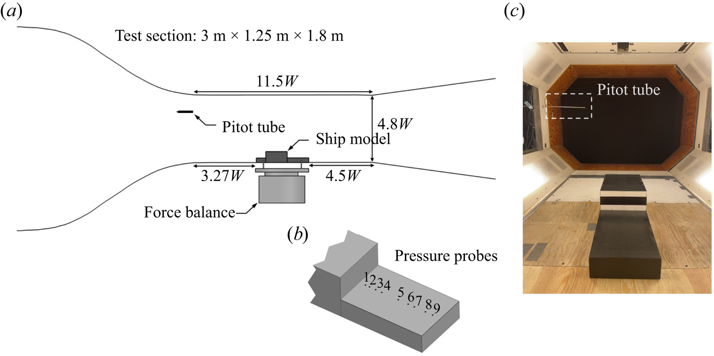
Figure 2. Experimental set-up. (a) Schematics of Chalmers L2 Wind Tunnel from the side view with the test section normalized by model width ( $W$). (b) Locations of pressure probes on the deck of the baseline ship model. (c) Picture of wind tunnel inside.
The pressure measurements are conducted using a differential pressure scanner 9116 with a scanning frequency of 62.5 Hz and a sampling time of 60 s. The pressure distribution is obtained by the pressure probes located along the centre of the deck, as shown in figure 2(b). Table 1 presents the specific positions of probes relative to the base.
Table 1. Locations of pressure probes ( $x/W$).
The pressure coefficient is obtained based on the measured pressure using (2.2)
 \begin{equation} C_p = \frac{p-p_{\infty}}{0.5\rho_{\infty}{U_{\infty}}^2}=\frac{\Delta p}{q_\infty} , \end{equation}
where  $p$ is the measured pressure on deck and $p_{\infty }$ is the free-stream pressure.
The total uncertainty,  $\epsilon _\xi$, is calculated following ISO 17025 (IOS 2008) and ASME PTC 19.1 (ASME International 2004), where Talyor expansions are used for error propagation as shown in (2.3). Each individual uncertainty $\delta x_i$ is assumed to be normally distributed and non-correlated
 \begin{equation} \epsilon _\xi(x_1, x_2,\ldots, x_n) = \left\{\sum_{i=1}^{n} \left( \frac{\partial \xi}{\partial x_i} \cdot \delta x_i \right)^2 \right\}^{1/2}, \end{equation}
where  $\xi$ is a dependent variable, $n$ is the number of independent variables $x_i$ applied to in (2.1) and (2.2) and $\delta x_i$ is the relevant error. It is worth mentioning that, due to the low-speed nature of the experiments, extra precautions were taken to mitigate bias errors. All devices were re-zeroed between each consecutive experimental data point at $0\ {\rm m}\ {\rm s}^{-1}$ wind speed in the tunnel test section. The zero drift between each data point for PSI-9116, FCO510 and the 6-axis balance was mitigated by multiple re-zeroing until the drift is within a specified range. The uncertainty of the pressure readings from the differential PSI-9116 and FCO 510 are assessed to be 0.215 pa and 0.05 pa, based on in situ calibration by an FCO-560 micromanometer accredited following ISO 17025 to 0.1 % or reading three significant digits. The wind tunnel temperature is accredited to an uncertainty of 0.3 K and ambient pressure of 0.1 %. The projected frontal area of the model was measured with a Mitutoyo calliper with an uncertainty of 0.07 mm and is assumed to have straight edges. The uncertainty assessment of the force balance is based on the repeatability of identical tests and weight calibrations, resulting in 0.012 N uncertainty. The uncertainty estimation does not account for cable interference on the balance nor any flow in the slit around the model.
3. Numerical methods and validations
The LES is conducted using the commercial finite volume software, Star-CCM+. The governing equations are the incompressible, spatially filtered three-dimensional Navier–Stokes equations, which keep the unsteadiness associated with the large-scale turbulent motion and model the small-scale high-frequency components of the fluid motion. The filter width,  $\varDelta$, is associated with the cell size and is defined as $\varDelta = (\varDelta _i\varDelta _j\varDelta _k)^{1/3}$. The WALE model proposed by Nicoud & Ducros (Reference Nicoud and Ducros1999) is employed in the present study to provide the subgrid-scale viscosity ( $\mu _t$) in the Boussinesq approximation of the subgrid-scale stress tensor. The WALE model has been validated in our previous numerical study on the same ship model (Xu et al. Reference Xu, Su, Bensow and Krajnović2022, Reference Xu, Su, Bensow and Krajnovic2023a,Reference Xu, Su, Xia, Wu, Bensow and Krajnovicb). It has also been extensively validated in predicting flows around the hatch-back (Aljure et al. Reference Aljure, Lehmkuhl, Rodriguez and Oliva2014), the square-back (Dalla et al. Reference Dalla, Evstafyeva and Morgans2019) and the notch-back (He et al. Reference He, Minelli, Wang, Dong, Gao and Krajnović2021) Ahmed bodies that resemble the bluff-body shape of the current ship model. The WALE model is, therefore, suitable for the current numerical study. The WALE model computes the subgrid eddy viscosity based on the invariants of the velocity gradient and accounts for the rotational rate. It is defined as
 \begin{equation} \mu_t=\rho (C_w \varDelta)^2 \frac{(S_{ij}^* S_{ij}^*)^{3/2}}{(\tilde{S}_{ij} \tilde{S}_{ij})^{5/2}+(S_{ij}^* S_{ij}^*)^{5/4}} , \end{equation}
where the model coefficient  $C_w$ is 0.544. Here, $\tilde {S}$ is the strain rate tensor computed from the resolved velocity field and $S_{ij}^*$ is the traceless symmetric part of the square of the velocity gradient tensor, defined as
 \begin{equation} S_{ij}^* = \tfrac{1}{2}(\tilde{g}_{ij}^2+\tilde{g}_{ji}^2)- \tfrac{1}{3}\delta_{ij}\tilde{g}_{kk}^2, \end{equation}
where  $\delta _{ij}$ is the Kronecker delta and $g_{ij}= \partial u_i/ \partial x_j$.
The convective flux is evaluated by a bounded central differencing scheme that blends 98 % of the second-order central differencing scheme and 2 % of the first-order upwind scheme for robustness purposes. The implicit unsteady solver with a second-order Euler implicit scheme is used to approximate the transient term. The physical time step ( $\Delta t$) is set to $1.443\times 10^{-4}$ s, which ensures that the Courant–Friedrichs–Lewy number is lower than 1 in over 99 % of the cells. The LES simulation starts from a preliminary flow field provided by an unsteady Reynolds-averaged Navier–Stokes (URANS) simulation with $k-\omega$ SST turbulence model, where k is turbulence kinetic energy, $\omega$ is the specific rate of dissipation and SST is shear stress transport. After a characteristic time ( $t^*=tU_\infty /h$) of 65, when all the aerodynamic forces become dynamically stable, LES simulation begins sampling and averaging results for $t^*$ of 1142. The present LES simulation is conducted using the Tetralith general computing resource provided by SNIC (Swedish National Infrastructure for Computing) at the National Supercomputer Center (NSC). Each case requires about 244224 CPU hours and 768 cores (Intel Xeon Gold 6130 processors).
Figure 3 shows the computational domain with a cross-sectional area of  $6.5 {W} \times 5 {W}$, which accounts for a blockage ratio of approximately 2.4 %. The length of the domain is 28 $W$ with 8 $W$ from inlet to bow tip point and 16 $W$ from stern to outlet. The ship model sits on the floor with no gap in between. The coordinate system and velocity direction are denoted by $x$ and $u$ in the streamwise direction, $y$ and $v$ in the spanwise direction and $z$ and $w$ in the vertical direction. Since the wind tunnel has a low turbulent level of less than 0.5 %, the velocity inflow boundary condition with a uniform free-stream velocity of $U_\infty = 5\ {\rm m}\ {\rm s}^{-1}$ is specified at the inlet, and no particular treatment is conducted for the free-stream turbulence. The free-stream boundary layer profiles extracted from points a, b and c (located at 6.4W, 3.7W, and 2.7W ahead of the ship) are shown on the right of figure 3. A static pressure outlet boundary condition is applied at the outlet. The top and sides of the domain are specified with the symmetry boundary condition. The no-slip wall boundary condition is applied on the floor and all ship surfaces. Note that the size and shape of the computational domain and the choice of symmetry boundary condition are reasonably adjusted from the experiment, which marginally varies the numerical results. The intention is to facilitate meshing and reproduce the testing conditions at a lower computational cost.

Figure 3. Computational domain (normalized by model width) and free-stream boundary layer profiles extracted at locations of a, b and c to show the boundary layer development.
The structured hexahedral mesh is created using Pointwise. Figure 4 shows the details of the mesh topology. The initial mesh size contains 37 million cells for the baseline model and 38 million cells for the FR model. Based on various numerical studies (Zhang et al. Reference Zhang, Minelli, Rao, Basara, Bensow and Krajnović2018; Rao et al. Reference Rao, Zhang, Minelli, Basara and Krajnović2019; Zhang et al. Reference Zhang, Minelli, Basara, Bensow and Krajnović2021) on ships with a grid size ranging from 6 to 21 million cells, a grid size of 37 million cells for the present study is expected to be sufficient. The near-wall grid distance  $\Delta y$ is $3\times 10^{-5}\ {\rm m}$, which ensures $y^+={\Delta y u_\tau }/{\nu }$ lower than 1. For the resolution in the streamwise ( $\Delta s^+={\Delta s u_\tau }/{\nu }$) and spanwise ( $\Delta l^+={\Delta l u_\tau }/{\nu }$) directions, $\Delta s^+$ is less than 55 and the maximum $\Delta l^+$ is 21, which satisfies the suggested ranges proposed by Piomelli & Chasnov (Reference Piomelli, Chasnov, Hallbäck, Henningson, Johansson, Alfredsson and Henningson1996). Furthermore, as shown in table 2, a grid dependency study with $t^* \approx 200$ is conducted on the baseline CSM using a coarse mesh of 27 million cells and a fine mesh of 47 million cells. The metric $L_R$ measures the reattaching distance on deck at the symmetric plane and the maximum deviation ( $\Delta L_R$) is 3.13 %. The acquired drag coefficients ( $C_D$) fall in a very close range with the deviation ( $\Delta C_D$) from the initial mesh of less than 0.9 %. It also shows that $C_D$ acquired by the initial mesh is more consistent with the fine mesh, which suggests the convergence of solutions to the fine mesh. Note that the predicted drag force is acquired by integrating the surface pressure and wall shear stress in the $x$ (free-stream) direction.

Figure 4. Mesh topology of the baseline CSM. (a) Ship surfaces. (b) Cross-section of the superstructure. (c) Normal to the bow. (d) Symmetry plane.
Table 2. Results of the grid dependency study, baseline case.
The numerical method is validated by comparing the drag force and  $C_p$ distribution with the experimental measurements. The initial mesh predicts $C_D$ of 0.562 as shown in table 2 and is 4.58 % deviated from the experimental value of $0.589\pm 0.015$. For reference, the aerodynamic drag can contribute up to 10 % of a ship's overall drag (water and air), depending on the aerodynamic shape.
Then, the  $C_p$ distribution along the centre of the deck (figure 2b) is used for further validation. Gauge pressure is used to calculate $C_p$ throughout the paper. Figure 5 shows the predicted and experimental $C_p$ distributions are in good agreement from the base ( $x/W=0$) to deck end ( $x/W=1.54$). The error bars on the figure reflect the total uncertainty from all measured quantities, which is evaluated using (2.3). The deck pressure first decreases to the minimum due to the re-circulation bubble and then the flow reattachment on the deck increases the pressure to the peak value. The parameter $\Delta C_p$ is the discrepancy between numerical and experimental results. Most of the high discrepancies are located within the flow separation region of $0 < x/W< 0.55$, which is usually challenging in flow predictions. Similar discrepancies at such a location are also reported in other ship research (Zhang et al. Reference Zhang, Minelli, Rao, Basara, Bensow and Krajnović2018, Reference Zhang, Minelli, Basara, Bensow and Krajnović2021). Figure 5 also shows that the predicted $C_p$ distributions acquired by the three meshes are virtually overlapped. It is indicated that the current numerical method is capable of predicting the flow around the CSM with satisfactory accuracy, and the result is converged on the initial mesh size of 37 million cells.

Figure 5. Baseline  $C_p$ distribution at the centre of deck. Error bars are acquired by error propagation analysis. The $C_p$ differences ( $\Delta C_p$) between LES initial and experiment are plotted by blue bars.
Furthermore, the grid dependency study is also conducted on the FR case. Table 3 presents the time-averaged  $\overline {C_D}$ on a $t^* \approx 200$ using the initial, coarse and fine meshes of $3.9\times 10^7$, $2.9\times 10^7$ and $4.8\times 10^7$ cells, respectively. The variation $\Delta \overline {C_D}$ among different sets of meshes is less than 1 %. The FR case has lower drag than the baseline because the rounded surfaces reduce the pressure stagnation on the ship's front surface. Figure 6 presents the mid-deck time-averaged $\overline {C_p}$ distributions for the three sets of meshes where $\overline {C_p}$ virtually overlaps. Both $\overline {C_D}$ and $\overline {C_p}$ distributions demonstrate that the solution is converged with the initial mesh. More grid dependency studies around the ship's superstructure are provided in the Appendix.
Table 3. Results of the grid dependency study, FR case.
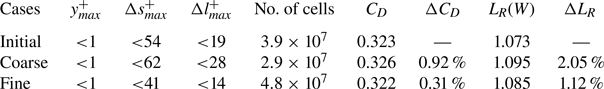

Figure 6. The FR  $C_p$ distribution at the centre of the deck.
4. Results and discussion
This section compares the flow fields between the baseline and front-shape-modified cases to study the wake bi-stability including its characteristics and persistence mechanism. Both cases are simulated at the headwind condition for a  $t^*$ of 1142, corresponding to a dimensional time of 26.5 s.
4.1. Flow characteristics
The modified CSM, referred to as the FR case, is created based on the baseline CSM by rounding the sharp-edge front to a quarter-ellipse shape, as shown in figure 7. The ellipse shape is kept the same among sides and roof with a semi-major axis ( $a$) of 0.09 $W$ and a semi-minor axis ( $b$) of 0.07 $W$, where $W$ is the ship's width. A small step with a width of 0.45 % $W$ is added to the ellipse curve to trigger corner eddies for better flow attachment on curved surfaces. The modified ship front, therefore, consists of three regions, as shown in figure 7(b): rounded roof surface (green), rounded side surfaces (orange) and main front (blue). Modifying the square edge to the ellipse shape causes a volume loss of the superstructure by 0.4 %.

Figure 7. Front-shape modifications. (a) Baseline model with sharp-edge front and the (b) FR case with a rounded front shape. A cross-section of the roundness is shown in the bottom right. The lengths of a and b are 0.09 $W$ and 0.07 $W$, respectively.
Similar to (2.1),  $C_x$ is defined as the coefficient of the $x$-directional force integrated using the surface pressure. The histories of $C_x$ on base surfaces of the baseline and FR CSMs are shown in figure 8, where the left and right sides are coloured orange and blue, respectively. The negative sign indicates a suction force opposite to the free-stream direction, which increases the drag force. As shown in figure 8(a), the total force ( $\varSigma C_x$) of the entire base surface in the FR case is 19.5 % lower than it is for the baseline case due to vortex-induced pressure reduction on the base. More discussion will be provided later.

Figure 8. Histories of  $x$-force coefficients ( $C_x$) on the base surface of the ship. The baseline case is coloured in red and FR is in black. (a) Total $x$-force coefficient $\varSigma C_x$ on the base. (b) Baseline lateral difference ( $\Delta C_x$) showing random and frequent switches. (c) FR lateral difference showing an asymmetric wake with a switch attempt. (d) Power spectrum densities of $\Delta C_x$.
In figure 8(b), the baseline case has  $\Delta C_x$ constantly switching between the left and right sides, labelled as the L-state and the R-state. There are seven switches, with intermediately near-zero $\Delta C_x$ between left and right. The maximum $t^*$ that the wake stays on one side is 172, which is significantly lower than $t^*$ of 400–1000 for a bi-stable wake (Grandemange et al. Reference Grandemange, Gohlke and Cadot2013b; Volpe et al. Reference Volpe, Devinant and Kourta2015; Barros et al. Reference Barros, Borée, Cadot, Spohn and Noack2017). The probability density functions (PDFs) present a spread shape, confirming the unstable nature of the baseline wake. Since the baseline wake has two preferred states but frequently switches states, it is regarded as weak bi-stability. For the FR case in figure 8(c), the $\Delta C_x$ presents a concentrated single spike, indicating an asymmetric and stable wake. It is worth noting that a switch attempt is captured towards the end of the history where the wake switches its state for a short $t^*$ of 32 and quickly switches back. This suggests that the FR wake may not be the perfectly stable asymmetric wake after the first bifurcation, as described in Grandemange et al. (Reference Grandemange, Cadot and Gohlke2012), but is possibly one of the RSB states of a potential bi-stable wake. This is further confirmed through POD analysis later. Figure 8(d) shows the power spectral densities (PSD) of the lateral difference of $x$-force coefficients ( $\Delta C_x$). The $-2$ (Grandemange et al. Reference Grandemange, Gohlke and Cadot2013b; Pavia, Passmore & Sardu Reference Pavia, Passmore and Sardu2018) law depicting the logarithmic decrease of the energy indicates that the asymmetric wake in the FR case can be one of the two states of a possible bi-stable wake. Moreover, the $-7/3$ law reported by Volpe et al. (Reference Volpe, Devinant and Kourta2015) is also observed here, suggesting the eddy motions are in the inertial range (Batchelor Reference Batchelor and Green1951; Hill & Wilczak Reference Hill and Wilczak1995).
Figure 9 plots the lateral pressure gradients  $\partial C_p/ \partial y$ against the vertical pressure gradients $\partial C_p/ \partial z$. The pressure gradients are calculated by (4.1) and (4.2), respectively, using the instantaneous pressure acquired at four probe locations of A, B, C and D in figure 9
 \begin{gather} \frac{\partial C_p}{\partial y} = \frac{[C_p(A)+C_p(D)]/2-[C_p(B)+C_p(C)]/2}{\Delta y/W} , \end{gather}
 \begin{gather}\frac{\partial C_p}{\partial z} = \frac{[C_p(A)+C_p(B)]/2-[C_p(C)+C_p(D)]/2}{\Delta z/W} . \end{gather}
Figure 9. Probability density function of lateral ( $\partial C_p/ \partial y$) and vertical ( $\partial C_p/ \partial z$) pressure gradients of (a) baseline and (b) FR, showing the switching nature of the baseline wake and the asymmetric FR wake. Here, $\Delta y$ and $\Delta z$ measure the lateral and vertical distances between probe locations.
The baseline case has a flat-shaped distribution with the highest probability density occupying both sides, supporting the statement that the wake is laterally switching between two positions. The FR case's probability density appears only on the left, which reflects the laterally asymmetric wake. Besides, distributions of  $\partial C_p/ \partial z$ in both cases are approximately symmetrical about a value slightly lower than 0 (marked by the dashed-dot line). This means the wake is relatively stable in the vertical direction ( $z$) and has no vertical switch.
To illustrate the lateral pressure difference, figure 10 shows contours of the time-averaged pressure coefficient ( $\overline {C_p}$) on regions of the ship base, deck and stern. The distributions of vortex cores are marked by the yellow lines and pressure iso-surfaces (coloured by the $\overline {C_p}$ contour colour) are at $\overline {C_p}=-0.3$ and $-0.12$ behind the base and stern, respectively. The baseline case has its vortex cores and iso-surfaces symmetrically distributed, whereas the FR case presents a lateral asymmetry. To facilitate discussion, the vertical sections of the vortex core are named vortex roots, as shown in figures 10(a) and 10(b). For the flow immediately downstream of the base, vortex roots of the baseline case are at similar axial locations with a slight difference of 0.01 $W$. This location difference is significantly increased to 0.26 $W$ in the FR case with the right side closer to the base. As such, the pressure is reduced differently, leading to the lateral pressure asymmetry on the surfaces of the base as well as the deck. Moreover, the size of the low-pressure zone is also enlarged at the near-base side, as indicated by the $\overline {C_p}$ iso-surface in figures 10(b) and 10(d), which not only enhances the lateral pressure differences but also further reduces the base pressure. This explains the 19.5 % lower $\overline {C_x}$ observed in the FR case. Although the FR case has a higher suction force at the base, its rounded front shape significantly reduces the stagnation pressure at the front surface, leading to the overall low drag in table 3.

Figure 10. Pressure coefficient ( $\overline {C_p}$) contours at the base, deck and stern surfaces. Iso-surface of $\overline {C_p} = -0.3$ (behind the base) and $-0.12$ (behind the stern). Distributions of vortex core (coloured by yellow) with the vertical section being regarded as the vortex roots. (a,c) Show the baseline case in the three-dimensional view and top view and (b,d) show the FR case in the three-dimensional view and top view.
Figure 11 shows the mean flow structures of the two cases using distributions of vortex cores (orange lines) and two-dimensional streamlines in planes at  $z=0.08W$, 0.49 $W$ and $y=0W$. The top-right figures are the front view of each case. The flow re-circulation zones are illustrated by the grey iso-surfaces at $\bar {u}=0$. All velocities ( $\bar {u}$ and $u$) are normalized by the free-stream velocity ( $U_\infty$). Above the ship's bow, the most upstream structure is the bow leading-edge vortex (BLEV) observed at the tip of the bow. Downstream of the BLEV there is a larger vortex structure, the bow-top vortex (BTV), which extends laterally across the ship's front, induced by the blockage from the bluff-shaped superstructure front. Both ends of BTV in the baseline case stop developing downstream due to the blocking from sharp side edges, whereas the rounded side surfaces in the FR case allow the BTV to slide over and flow downstream, turning into superstructure-side vortices (SSV). The front corner eddies (FCE) are observed at the edge between the front and bow-top surfaces, and have a short extension ( $FCE_{ex}$) passing the front side edges in the baseline case. At this location, bow-side vortices (BSVs) are observed at each side of the bow. Around the ship's superstructure front, front vortices (FVs) are generated due to flow separating from the roof and side edges. The baseline case with the sharp edges has a remarkably more severe flow separation than the FR case as shown by the iso-surface of $\bar {u}=0$ and the streamlines in figure 11(a). The reattached velocity profiles are significantly fuller in the FR case, as shown by figure 12. These are the major differences caused by front-shape modifications. Figure 12 also compares the turbulent kinetic energy (TKE, normalized by
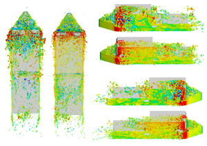
  ${U_\infty }^2$), where the baseline case has much higher TKE than the FR case due to the front flow separation. This is aligned with the finding in Ahmed & Morgans (Reference Ahmed and Morgans2023). Moreover, FVs are also induced by the flow separation at sharp-edged adjunctions between the surfaces of bow sides and ship sides. In the downstream behind the base, a horseshoe-shaped vortex structure is observed for both cases, which is a typical structure on the flight deck of ships, as discovered by Shafer & Ghee (Reference Shafer and Ghee2005). The flow separates at the roof trailing edge, causing the re-circulation behind the base shown by the re-circulation zone (RZ) in figure 11. Additionally, flow also separates at both sides of the ship, inducing a pair of counter-rotational vortices (CVs), contributing to the formation of the horseshoe shape. The FR case has the near-base-side CV in a circular shape and is larger than the other side with a stretched shape. This aligns with the previous observations in figure 10 that the near-base side has a stronger vortical flow. Similar findings are also reported by Herry et al. (Reference Herry, Keirsbulck, Labraga and Paquet2011). Such shape patterns of CVs will be used in § 4.2 to identify the asymmetric wake, especially in its early stage. Downstream of the stern, the same horseshoe-shaped vortex can be observed in both cases due to the same flow phenomena discussed above. It is noteworthy that the two horseshoe vortices in the FR case are anti-asymmetrically distributed, as shown in figure 11(b); in other words, the R-state structure behind the base is associated with the L-state structure behind the stern. Since the two structures are asymmetrical in an opposite way, they are termed the anti-asymmetrical structure. Such a flow phenomenon is also reported by Rao et al. (Reference Rao, Zhang, Minelli, Basara and Krajnović2019) and Khan et al. (Reference Khan, Parezanović and Afgan2023), however, the underlying cause seems to be insufficiently discussed. In this regard, a more detailed explanation is provided as follows.

Figure 11. Flow structures of (a) baseline case and (b) FR case. Two-dimensional streamlines at planes of  $y=0$, $z=0.49W$ (behind the base), and $z=0.08W$ (behind the stern) showing the wake asymmetry difference and the different flow separations in the front; distributions of vortex cores (coloured blue) including BLEV, BTV, BSV, SSV, FVs and CVs. Iso-surface at $\bar {u}=0$. Front view of the two cases at the top right.

Figure 12. Velocity and TKE profiles on the left (a), roof (b) and right (c) surfaces of the superstructure. The extraction points are marked in figure 11(a), at 1.16 $W$ downstream of the ship's front. The right extraction point is symmetric to the left.
Figure 13 shows the time-averaged  $y$-vorticity ( $\overline {\omega _y}$) with two-dimensional streamlines at two lateral planes of $y=\pm 0.19 W$ (left and right), labelled as $y_L$ and $y_R$. Planes $y=\pm 0.19 W$ are chosen to ensure that they are located sufficiently away from the centre and, at the same time, cut through the lateral section of the vortex core as well, which facilitates the comparison of the lateral difference. For quantitative analysis, $\alpha$ defines the angle between the $y$-vorticity sheet and the horizontal, and $L_R$ is the distance of the reattachment point on the deck. An obvious asymmetry is shown in figures 13(a) and 13(b). The parameter $\overline {\omega _y}$ on the plane $y_R$ is more vectored towards the deck as compared with the left and the $\alpha$ angle is increased by 71.1 %, leading to a stronger induction effect on the main flow for energizing the low-speed re-circulating region behind the right side of the base. As a result, the vortex core is pushed downwards, ending up 24.7 % lower than the left side, and the reattachment length $L_R$ is shortened by 21.2 %. Since the flow reattaches earlier on the right side, it has a longer deck distance to recover its $u$ velocity, which results in a higher velocity upon reaching the deck trailing edge. This can be supported by figure 13(c), plotting the time-averaged streamwise velocity ( $\bar {u}$) profiles that are extracted from planes $y_R$ and $y_L$ at the trailing edges of the deck (black dashed lines). The $\bar {u}$ profile at the right side with earlier reattachment is significantly fuller than the left. As the high-velocity (high-momentum) flow separates at the stern, it can travel farther downstream before being re-circulated, generating a stretched and enlarged re-circulation region with the vortex core positioned away from the stern. This is why the near-base side of the horseshoe vortex (earlier attachment) is always associated with the away-from-stern side (stretched re-circulation) in the downstream. On the left, the low-velocity flow separating from the stern leads to the opposite structure. The aforementioned anti-asymmetrical vortex structure is therefore explained. Figure 13(c) also plots the TKE profiles upstream of the stern. Note that the lateral difference of TKE is an order of magnitude smaller than that of $\bar {u}$. The fluctuating quantities may not play an important role in shaping the stern wake. In other words, the asymmetry of the stern wake is the consequence of mean-quantity asymmetry behind the base. To better assist the understanding, figure 13(d) uses the representative streamlines to illustrate the main patterns of the anti-asymmetrical vortex structure.

Figure 13. Time-averaged  $y$-vorticity ( $\overline {\omega _y}$) at two lateral planes of $y=\pm 0.19 W$, (a) left and (b) right. The centres of the re-circulation regions are marked, showing a strong lateral difference. Here, $\alpha$ is the angle between the $\overline {\omega _y}$ sheet and horizontal and $L_R$ is the distance of the reattaching point to the base surface. (c) Shows the profiles of $\bar {u}$ and TKE extracted at the deck trailing edge, showing the flow quantities upstream of the stern. The extraction location is shown in (a). (d) Shows a sketch of the representative streamlines at the left and right to demonstrate the re-circulation regions behind the base and behind the stern in the left and right planes.
To focus on the flow characteristic of the L-state and R-state separately, conditional averaging is conducted for the velocity and shear stress at plane  $z=0.49W$. Figure 14 compares the separated L-state and R-state baseline wake with the FR wake. White iso-lines mark $\bar {u}=0$ for the re-circulation region. The L-state FR wake is acquired by data asymmetry for better comparison. In the FR case, the two lateral re-circulation regions present a distinguished shape difference as the dominant one is circular and the constrained one is more stretched. Alternating wake states under such a significant difference will require significant efforts, for example, a strong upstream disturbance from boundary layer separation (Ahmed & Morgans Reference Ahmed and Morgans2023). Comparatively, the baseline's re-circulation regions possess a slight lateral difference and are therefore prone to alternation. The alternation can be further facilitated in the baseline case due to the strong upstream disturbance generated from the sharp-edge flow separation, as shown in figure 11. These factors lead to the frequent-switching behaviour in the baseline case. Another fact can be observed through the shear stress ( $\overline {u'v'}$, normalized by ${U_\infty }^2$), as shown in figure 14. The FR case has a more elongated re-circulation region than the baseline case. The FR's shear layers, therefore, have a small curvature, whereas those of the baseline case possess a high curvature, as highlighted in purple dashed lines. Since the curvature increase can lead to the growth of the shear layer instability (Liou Reference Liou1994), the baseline wake is more subjected to upstream disturbance with a frequent-switching feature.

Figure 14. Conditional averaging results of  $\overline {u}$ and $\overline {u'v'}$ contours at $z=0.49W$. (a–d) Show the baseline case. (e–h) Show the FR case. RZs are coloured by white iso-lines of $\bar {u}=0$. The $\bar {u}$ contours show a stretched bubble shape of the FR case with a pronounced lateral difference between the lateral re-circulation regions and the $\overline {u'v'}$ contours show that the baseline shear layers have higher curvature than the FR case. Purple dashed lines highlight the shear layer curvatures.
For a better understanding of the wake dynamics, POD is conducted in the velocity field at the  $z$-plane $z=0.49W$. Note that data symmetry is conducted to both cases to make the POD basis comparable. The data sampling time is approximately $t^*=1142\times 2$ with a sampling frequency of 690 Hz. The data processing routine follows the practice by Östh et al. (Reference Östh, Noack, Krajnović, Barros and Borée2014). The sampling frequency of 690 Hz corresponds to ten times the time step ( $1.443\times 10^{-4}$) used in the simulation, which leads to the highest reliable frequency (Nyquist frequency) of 345 Hz, $St_H (fW/U_\infty )=17.94$. Figures 15(a) and 15(d) show the energy fraction of the first ten modes of the two cases. Both cases have their first mode dominating the entire energy content. The spatial distribution of this mode is shown in figures 15(b) and 15(e) with an asymmetric pattern. The two distinct regions demonstrate the shifting of streamwise momentum. This aligns with the observations in Pavia et al. (Reference Pavia, Passmore, Varney and Hodgson2020), Fan et al. (Reference Fan, Xia, Chu, Yang and Cadot2020) and Aleyasin, Tachie & Balachandar (Reference Aleyasin, Tachie and Balachandar2021), which is typically considered the responsible mode for the bi-stable wake. It is noteworthy that the first mode energy percentage of the baseline is 71 % lower than the FR case, which supports the fact that the baseline case has a weak bi-stability. Further evidence can be observed in the PSD of the temporal coefficient of the first mode in figures 15(b) and 15(e). The repartition of energy for low frequency in the FR case follows a power law with an exponent close to $-2$, confirming the bi-stable feature. Comparatively, the baseline case presents a different energy repartition for low frequency as a weak bi-stability. Figures 15(c) and 15(f) are spatial distributions of the vortex shedding mode for the baseline and FR cases, respectively. Four distinct regions are observed with the existence of lateral and longitude asymmetry, indicating the shedding behaviour. The PSD of the temporal coefficient suggests that the FR case has a dominant frequency $St_H$ of 0.171, which is consistent with the typical shedding frequency found for a buff body (Grandemange et al. Reference Grandemange, Gohlke and Cadot2013b). Comparatively, the dominant frequency in the baseline case is significantly higher at 0.218, indicating the shedding activities are more vigorous and frequent. This, again, aligns with the unstable feature of the baseline wake.

Figure 15. The POD analysis based on the velocity field at plane  $z=0.49W$. The energy fraction of the first ten modes is shown in (a,d). Spatial distributions of the first mode are shown in (b,e). The FR case follows a power law of $-2$ in the low-frequency regime. Spatial distributions of the fourth mode of the baseline case and the third mode of the FR case are recognized as the shedding mode, and are shown in (c,f). The high shedding frequency in the baseline case aligns with its unstable feature. (a–c) Are the baseline case. (d–f) Are the FR case.
4.2. Discussion on the persistence mechanism of the bi-stable wake
Maintaining a stable and asymmetric structure in either of the two preferred states is a key feature for the bi-stable wake, and this section is dedicated to understanding the mechanism of this feature. As demonstrated in § 4.1, the baseline wake has a weak bi-stability with frequent switches between the R-state and L-state, and is sustained for less than 180 $t^*$ in each state, which constantly flips the sign of the lateral pressure gradient on the base surface. This can be a consequence of the different streamwise locations of the vortex roots, the vertical section of the horseshoe vortex core on deck, as shown in figure 10. When one side of the vortex root moves closer to the base than the other, the lateral pressure gradient appears, similar to the situation in figure 10(b). As the two sides of the vortex roots alternatively approach the base and move away from the base, the lateral pressure gradient switches. With the sharp edges rounded in the FR case, however, the vortex core persists in an asymmetric position with the right side root ahead of the left. In this regard, the key to understanding the persistence mechanism is to connect the link between shape modifications and vortex root movements. In other words, the question of interest here is how shape modifications affect the downstream vortical activities that lead to different wake behaviours (switching and persisting).
Understanding vortical activities in the wake can be approached by analysing the variation of vorticity. This is based on the fact that a high vorticity magnitude can indicate local vortex motions. In fact, a vortex identification method has been developed utilizing the local vorticity maximum (Strawn, Kenwright & Ahmad Reference Strawn, Kenwright and Ahmad1999). For the current case, since the vortex roots are  $z$-directional vortical flows, we confined our interest in $z$-vorticity ( $\omega _z$) activities at the $x$–
$x$– $y$ plane normal to the vorticity vector.
To have a preliminary understanding of how front-shape modifications affect  $\omega _z$, figure 16 shows the time-averaged $z$-vorticity ( $\overline {\omega _z}$) contours of the two cases at the $z=0.49W$ plane. A noticeable difference observed is that the baseline case has high-magnitude vorticity originating from the superstructure's left and right leading edges (LEs), which is due to the severe flow separation at sharp edges, as shown in figure 11(a). The FR case has mitigated vorticity magnitude along the ship sides. To quantify regional vorticity differences, table 4 presents the circulation ( $\varGamma$) evaluated based on Stokes’ theorem ( $\varGamma =\oint {\boldsymbol {v}} \boldsymbol {\cdot } {\rm d}{\boldsymbol {l}}=\iint \omega \boldsymbol {\cdot } {\rm d}{\boldsymbol {S}}$) at four regions of interest $UR_L$, $UR_R$, $DR_L$ and $DR_R$ (enclosed by dashed rectangles), located at two streamwise positions. It is demonstrated in both cases that the circulation is high upstream and gradually dissipates downstream and that the circulation is similar between left and right regions at the same streamwise location. For comparison, the baseline case has 275 % higher circulation than the FR case in the upstream at $UR_L$ and $UR_R$, and even with dissipation along ship sides, the circulation is still 45 % higher in regions $DR_L$ and $DR_R$. The high upstream vorticity in the baseline case is associated with a symmetric mean wake due to frequent switches. The vorticity sheets emanating from both sides of the superstructure trailing edges (STEs) are tilted in a similar $\beta$. These vorticity sheets are named STE vorticity sheets or base-side vorticity sheets. Comparatively, the FR case with reduced upstream vorticity maintains laterally different STE vorticity sheets. Regarding how STE vorticity sheets behave in different magnitudes of upstream vorticity, further investigation is continued in the time series as follows.

Figure 16. Time-averaged  $z$-vorticity ( $\overline {\omega _z}$) at $z=0.49W$ of the (a) baseline case and (b) FR case. Here, $UR_L$, $UR_R$, $DR_L$ and $DR_R$ are four regions of interest for circulation comparison and $\beta$ is the angle between $\overline {\omega _z}$ and the free stream. Here, TE stands for trailing edge.
Table 4. Circulation ( $\varGamma$) of four regions of interest.
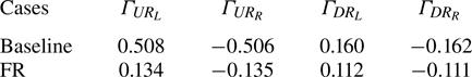
The POD analysis is conducted on the  $\omega _z$ field at plane $z=0.49W$ where the regions near the STE and behind the base are included. The data are sampled over a $t^*$ of 1142 with a frequency of 690 Hz. Data symmetry is not conducted to distinguish the laterally different motions. Figures 17 and 18 show the spatial distributions ( $\varphi$) of the first four modes of the two cases. The baseline case is dominated by the first four modes of motion with small correlated regions (mode 3) and anti-correlated regions (mode 4) observed at STE. However, most regions, including those behind the base and slightly away from STE, have a close-to-zero $\varphi$ value. Such a value suggests a low relevant dynamics, meaning that the regions have neither correlated nor anti-correlated motions. The PSD of the temporal coefficient presents a flat-shaped distribution in $St_H<1$ with no obvious spike region, meaning that energy is de-concentrated instead of condensing to a dominant frequency range. This also supports the random vorticity dynamics. Comparatively, the FR case has remarkably larger relevant regions (non-zero $\varphi$ value), especially on the left side with a stretched bubble shown in figure 11. The FR case is dominated by the first mode which indicates a lateral sweeping motion of the left vorticity sheet. This suggests the unstable nature of the left stretched bubble (Haffner et al. Reference Haffner, Borée, Spohn and Castelain2020). The anti-correlated regions appear alternatively in the second mode, and with its $St_H$ approximating to the typical shedding $St_H$ of 0.17, this mode represents the vorticity activities associated with vortex shedding.

Figure 17. The POD analysis based on the  $\omega _z$ field at plane $z=0.49W$ of the baseline case. (a) Is the energy fraction of the first ten modes. (b–e) Are the spatial distribution and temporal coefficients of the first four modes, demonstrating low relevant region (with neither correlated nor anti-correlated motions) with a flat-shaped PSD.

Figure 18. The POD analysis based on the  $\omega _z$ field at plane $z=0.49W$ of the FR case. (a) Is the energy fraction of the first ten modes. (b–e) Are the spatial distribution and temporal coefficients of the first four modes, demonstrating comparatively high relevant regions in the wake.
Overall, the comparison of the  $\omega _z$ POD suggests that the baseline case has virtually irrelevant or random $\omega _z$ activities in the wake region. This is especially aligned with the random switching pattern of vortex roots or wake states, as shown in figure 8. In contrast, the FR case with mitigated upstream vorticity establishes more regulated $\omega _z$ activities with highly relevant motions, and therefore tends to form a more stable vortex structure. Now the question becomes what exactly happens with these random $\omega _z$ activities in the baseline case that drives the motion of vortex roots and causes switches?
To demonstrate how vorticity activities vary during a switch, figure 19 shows the instantaneous  $\omega _z$ contours of the baseline case for six instants during a $t^*$ of 43, which covers a complete switch of wake from the R-state to L-state. The instantaneous static pressure contours and streamlines are also presented to show the wake characteristics at instants of interest. The contours and streamlines are extracted from the $z=0.49W$ plane, the same one as in figure 16. The histories of $C_p$ representing the left and right halves of the base are shown at the bottom of figure 19. As indicated by the magnitude of the lateral $C_p$ difference, the selected instants correspond to representative wake states, which include the (a) clear R-state, (b) weak R-state, (c) neutral state, (d) switch onset, (e) weak L-state and (f) clear L-state. The $C_p$ is extracted from the two probes shown in the middle of figure 19(a), positioned at the centre of the left and right halves of the base surface at $z=0.49W$.

Figure 19. Instantaneous  $\omega _z$ and $C_p$ contours of the baseline case at $z=0.49W$. (a–f) Are the six instants showing a complete switch of wake from R-state to L-state. Black arrows show the STE vorticity sheets’ movement directions. Dashed box encloses a tilted STE vorticity sheet in (a). Vortex root locations are marked by the square symbols and are connected by the white line in $C_p$ contours; $C_p$ histories are extracted from two probes located on the left and right sides of the base surface as shown in the $C_p$ contours of (a).
In all instants, large-scale  $\omega _z$ with high magnitude is observed emanating from the superstructure LEs and propagating downstream along the ship's sides, which is similar to the time-averaged results shown in figure 16. At instant (a), the low-pressure region behind the base is asymmetrically distributed with the right vortex core positioned ahead of the left (marked by the white line and squared symbols), which results in much lower $C_p$ on the right side, suggesting a clear R-state wake. Such a wake state is also evident by the streamlines where the dominant re-circulation region presents on the right and the streamwise-stretched one on the left. At this instant, the left side STE vorticity sheet (enclosed by the dashed box) is swept and tilted towards the deck centre, as highlighted by the black arrow, whereas the right side $\omega _z$ sheet develops downstream with no apparent inclination. As a result, the region downstream of the left base experiences increased vorticity with promoted vortical activities. In the subsequent instant (b), the left side re-circulated zone demonstrates an enlarged size with a less stretched shape, and the pressure gradient is more alleviated than the last instant because of the pressure reduction at the left side. The wake is developing to reach symmetry. With the vorticity still feeding to the downstream of the left base at instant (b), the wake becomes symmetric at (c), where the re-circulation region is balanced laterally, and the vortex cores are located at the same streamwise position. At this instant, neither side presents an apparent tilting of STE vorticity sheets. After a $t^*$ of 14, the balance is broken at instant (d) when the left side STE vorticity sheet is again tilted toward the deck centre, increasing the regional vorticity magnitude downstream of the left base. The left vortex core starts to move to the high $\omega _z$ region. Shortly after, at instant (e), a noticeable $C_p$ difference appears in the history plots with the opposite sign compared with (a,b). The re-circulation zones tend to have a stretched shape on the right and a dominated one on the left. At the final instant (f), the high vorticity feeds the near-base region from the left due to tilting, which locks the left vortex root near the base. The right side which has the high vorticity reaches further downstream, and the vortex core is therefore moved away from the base. A clear L-state wake is established as confirmed by the re-circulation regions’ shape and the enhanced $C_p$ difference.
Overall, it is demonstrated by the six instants that the motions of the vortex cores are driven by the  $\omega _z$ activities downstream of the base. As one side of the $\omega _z$ sheet is more tilted toward the deck centre, the regional vorticity magnitude is more enhanced than the other side, and the vortex cores end up with different streamwise positions for different wake states. Combined with the POD analysis of $\omega _z$, the switch of wake states possesses a strongly random pattern and is therefore randomly triggered by the tilting effect.
The proposed wake-switching mechanism based on the vorticity activities can be further supported in the FR case. Figure 20 shows the instantaneous  $\omega _z$ contours at six instants over $t^*$ of 43. Similarly, the pressure coefficient contours, instantaneous streamlines and the histories of $C_p$ are also presented. In all instants, the right side vorticity sheet is tilted to the deck centre. This is because the left side vorticity sheet has a more vigorous motion than the right side, as suggested by the POD analysis in figure 18(b). As was reported by Haffner et al. (Reference Haffner, Borée, Spohn and Castelain2020), the shear layer with an unstable vorticity sheet as the left side in the current study will remain more straight than the right side with a self-induced curving (tilting) movement. The more tilted vorticity sheet feeds a larger region behind the base with clockwise vorticity. As a result, the right side re-circulation region dominates the wake, regarded as the R-state wake. Compared with the baseline case discussed above, the FR case has significantly suppressed front flow separation with a reduced magnitude of $\omega _z$ in the upstream flow, as observed in all instants of figure 20. When the reduced $\omega _z$ flow approaches the STE, it still affects the STE vorticity sheets as the lateral sweeping motion represented by mode 1 in figure 18(b) can be observed here in figures 20(a) and 20(c), leading to the variation of relative positions of vortex cores (shown by the white line and symbols). But these variations are of a limited extent that is neither sufficient to switch streamwise positions nor alter the wake states. In other words, the random tilt of vorticity sheets is less commonly induced and the wake is tightened to a more stable structure. Furthermore, Fan & Cadot (Reference Fan and Cadot2023) experimentally found that a decrease in the viscous sublayer length scale ( $\delta _\nu =\sqrt {\nu /({\rm d}U/{\rm d}y_h|_{h=0})}$, $\nu$ being the kinematic viscosity of the flow) at the flow separation corresponded to a lower switching rate. This discovery aligns with the behaviour of the FR case in the current study whose boundary layer is significantly fuller at the near-wall location, as demonstrated in figure 12. Upon reaching the separation point at STE, ${\rm d}U/{\rm d}y_h|_{h=0}$ of the FR case is approximately 60 % higher than that of the baseline case. As a result, $\delta _\nu$ of the FR case is 79 % smaller, leading to a less switching wake.

Figure 20. Instantaneous  $\omega _z$ and $C_p$ contours of the FR case at $z=0.49W$. (a–f) Are the six instants showing a stable R-state wake with the right STE vorticity sheet more tilted than the left. Black arrows show the STE vorticity sheets’ directions of movement. Vortex root locations are marked by the square symbols and are connected by the white line in $C_p$ contours; $C_p$ histories are extracted from two probes located on left and right sides of the base surface as shown in the $C_p$ contours of (a).
To further demonstrate the upstream effect, figure 21 shows the iso-surface of the instantaneous  $z$-vorticity at a high magnitude of $\omega _z=\pm 400$ coloured by the instantaneous streamwise velocity $u$ from the top and sides views. It can be observed in the baseline case that the large-scale vorticity mass is induced at the ship front, whereas the vorticity scale in the FR case is significantly reduced due to the suppressed separation by the rounded front. Another consequence of the severe flow separation in the upstream is the reduced $u$ in the downstream. In the baseline case, the large-scale $z$-vorticity mass travels at a lower $u$. When vorticity sheets emanate from the trailing edges of the superstructure, a lower $u$ allows them to have more lateral movement with more tilting towards the deck centre. This is also confirmed by the $\beta$ angles and $\overline {\omega _z}$ distributions downstream the base in figure 16. In this way, the STE vorticity sheets have stronger effects on the vorticity activities in the wake flow, which assists in the triggering of vortex root switches.

Figure 21. Iso-surface of the instantaneous  $z$-vorticity $\omega _z=\pm 400$ coloured by instantaneous streamwise velocity ( $u$) with the views from the top (a,b), left side (c,d) and right side (e,f). (a,c,e) Are the baseline case showing the large-scale vorticity with low speed. (b,d,f) Are the FR case showing the small-scale vorticity with relatively high speed.
The current study created a flow-field comparison similar to Ahmed & Morgans (Reference Ahmed and Morgans2023), not through suction flow control but through front-shape modifications. Upon the suppression of the front flow separation, the frequently switching baseline wake is stabilized to a persistent asymmetric wake, which can be one of the RSB states of a potential bi-stable wake as suggested by the force history and POD analysis. This agrees with the key finding of Ahmed & Morgans (Reference Ahmed and Morgans2023) that the suppressed upstream disturbance results in a more stable wake. The difference is that their baseline wake is already bi-stable and separation suppression makes it further stabilized to a lateral symmetric state with the switching behaviour eliminated. At first glance, it appears that suppressing upstream separation promotes bi-stability in our case whereas it eliminates it in theirs, which may seem conflicting. However, the flow physics behind such a difference aligns since the two baseline wakes are stabilized to different states due to their different initial states. Moreover, Ahmed & Morgans (Reference Ahmed and Morgans2023) believe that upstream separation affects wake states by generating fluctuations and therefore their attention is focused on the effects of TKE. From an alternative aspect, the current study investigated how the upstream vorticity interacts with downstream wake flow. This is based on the fact that the boundary layer separation alters the vorticity sheets and that vorticity is closely linked with energy transfer and vortical activity. How the upstream vorticity behaviours interact with the downstream vorticity sheets behind the base and how the vorticity variations correlate with wake switching or lead to different wake states are the key contributions of the current study.
We recognize that the SFS2 model (Rao et al. Reference Rao, Zhang, Minelli, Basara and Krajnović2019; Mallat & Pastur Reference Mallat and Pastur2021; Zaheer & Disimile Reference Zaheer and Disimile2023) has a sharp-edged front but is well known for the bi-stable wake, which seems to behave contrary to the baseline case studied here. However, it is noteworthy that the superstructure of the SFS2 model is significantly longer than that of the baseline CSM, corresponding to a 3.28 times larger  $L/W$, where $L$ and $W$ are the length and width of the superstructure, respectively. Even though the high-magnitude $\omega _z$ is induced in the front, it is expected to be substantially dissipated before reaching the base of the SFS2 model, which will eventually behave as the FR case with a more stable wake. However, how much $L/W$ together with how strong vorticity is sufficient to cause constant wake switches are still open questions and need further study.
The current paper considers a perfect headwind, which is an ideal case to start with for studying different wake behaviours. The interest is, therefore, confined to the fundamental aspect of understanding the wake-persistence mechanism. In reality, a perfect headwind can be hardly experienced by ships, and their wake bi-stability is therefore strongly subjected to yaw effects. What is the minimum yaw angle that breaks the ship's bi-stable wake is a question of interest, and a topic worth studying in the future.
5. Conclusions
This paper numerically studies the wake characteristics of the CSM, aiming to understand the persistence mechanism of the bi-stable wake. The study uses LES with the WALE model. The experimental study is conducted to validate the numerical methods. Two cases are studied here: (i) the baseline CSM with a sharp-edged superstructure front and (ii) the FR CSM with sharp edges rounded to a convex shape.
During a sufficiently long time (characteristic time longer than 1000), the baseline wake has frequent switches, whereas the FR wake persists in an asymmetric structure with only one switch attempt. The PSD of the base surface force and POD analysis indicate the asymmetric wake in the FR case can be one of the two states of a potential bi-stable wake. The contours of surface pressure coefficients, streamlines and wake structures give more detailed flow characteristics of both cases. The base surface force is lower in the FR case due to the stronger vortical flow located closer to the base, reducing the base pressure. In the FR case, the wake structures behind the base and the stern are asymmetrical in an opposite way, and are therefore termed the anti-asymmetrical structure. It is found that such a particular wake structure downstream of the ship's base and stern is induced by the streamwise location variations of the reattachment points on the deck. The flow attaching earlier on the deck recovers a higher velocity upon reaching the deck trailing edge and induces stronger flow separation behind the stern. The flow attaching on the deck farther downstream leads to the opposite flow structure, which results in the anti-asymmetrical structure.
Furthermore, this paper proposes an explanation of wake-persistence/switching mechanism based on vorticity activities. The reasoning is carried out in three steps: (i) identify the overall difference in  $z$-vorticity ( $\overline {\omega _z}$) caused by front-shape modifications in the upstream; (ii) analysing how upstream ${\omega _z}$ activities affect downstream STE ${\omega _z}$ sheets in terms of their mode patterns; (iii) focusing on the instantaneous variation of STE ${\omega _z}$ sheets to study how it results in the switching or persisting wakes. It is found that the switching wake can be attributed to the occasional tilting of the (vertical-oriented) $z$-vorticity sheet at either side of the base toward the centre. As a result, the wake vorticity experiences a strong lateral variation that is sufficient to shift the streamwise positions of the vortex cores at the opposite lateral sides, which is observed as a wake switch. The tilting behaviour is subjected to the high-magnitude vorticity generated by the upstream flow separation at the front sharp edges and randomly initiates the wake switching. In the FR case, however, the upstream vorticity is mitigated due to the rounded front shape, and the tilting effect is significantly reduced. The downstream vorticity and vortex cores are therefore tightened to more stable structures, leading to the persisting asymmetric wake.
Funding
This work is supported by Chalmers University of Technology. The computations were enabled by resources provided by the National Academic Infrastructure for Supercomputing in Sweden (NAISS) at Tetralith partially funded by the Swedish Research Council through grant agreement no. 2022-06725. The authors also thank Chalmers L2 wind tunnel laboratory.
Declaration of interests
The authors report no conflict of interest.
Appendix. Additional results for mesh dependency study
This appendix provides additional mesh refinement results for both the baseline and FR cases. Time-averaged  $\overline {C_p}$ distributions are extracted along the left, roof and right surfaces of the ship's superstructure. This is to test the numerical credibility of predicting the flow around the ship's superstructure, which is important for the downstream wake prediction. Taking the baseline case as an example, extraction locations are shown in figure 22, where the base is located at $x/W = 0$ and the front surface is located at $x/W = -1.56$. The $\overline {C_p}$ distributions in the FR case are extracted downstream of the rounded surface. Results presented here use the same meshes as described in tables 2 and 3. The baseline case in figure 23(a) has a few sections of non-overlap at the separation and reattaching regions ( $-1.56 < x/W < -0.8$), which is due to the nature of prediction difficulty. As shown in figure 23(b), the FR case's $\overline {C_p}$ distributions overlap better than the baseline case. This is because the FR case has mitigated flow separation at the front, and the downstream flow becomes more steady, which is easier to predict. Overall, the $\overline {C_p}$ distributions of the baseline and FR cases demonstrate a good agreement among three sets of mesh, and the solution is converged with the initial mesh. The well-predicted flow around the superstructure benefits the wake prediction.

Figure 22. Illustration of  $C_p$ locations on the baseline ship's superstructure with (a) three-dimensional view and (b) top view.

Figure 23. The  $C_p$ comparisons at the ship's superstructure among the initial, coarse and fine meshes. (a–c) Are the baseline case. (d–f) Are the FR case.


 Open access