


1. Introduction
It has been more than 70 years since the phenomenon of polymer drag reduction in wall-bounded turbulence was first observed experimentally (Toms Reference Toms1948; Mysels Reference Mysels1949). Following this discovery, great efforts have been directed towards understanding how inertial turbulence (IT) is altered by the addition of polymers to the flow (e.g. see the reviews Lumley Reference Lumley1969; White & Mungal Reference White and Mungal2008). Polymeric fluids also exhibit counter-intuitive chaotic behaviour in very small-scale, inertialess flows. This ‘elastic’ turbulence (ET) was also first discovered experimentally (Groisman & Steinberg Reference Groisman and Steinberg2000, Reference Groisman and Steinberg2004) at vanishing Reynolds numbers and is thought to rely on finite-amplitude curvature in the streamlines (Shaqfeh Reference Shaqfeh1996). In contrast to polymer-modified IT, ET is associated with an increased drag relative to the laminar Newtonian state (Varshney & Steinberg Reference Varshney and Steinberg2018). It can be exploited to promote heat transfer (Traore, Castelain & Burghelea Reference Traore, Castelain and Burghelea2015) and to efficiently mix at very small scales (Squires & Quake Reference Squires and Quake2005).
In addition to these distinct phenomena, a third chaotic flow state was recently identified (Dubief, Terrapon & Soria Reference Dubief, Terrapon and Soria2013; Samanta et al. Reference Samanta, Dubief, Holzner, Schäfer, Morozov, Wagner and Hof2013) where both inertial and elastic effects are relevant, and was named ‘elasto-inertial’ turbulence (EIT). Elasto-inertial turbulence can be sustained for Reynolds numbers  $Re = O(1000)$, and is potentially linked to the ‘early turbulence’ reported in a range of experimental studies (Jones & Maddock Reference Jones and Maddock1966; Goldstein, Adrian & Kreid Reference Goldstein, Adrian and Kreid1969; Draad, Kuiken & Nieuwstadt Reference Draad, Kuiken and Nieuwstadt1998; Chandra, Shankar & Das Reference Chandra, Shankar and Das2018; Choueiri, Lopez & Hof Reference Choueiri, Lopez and Hof2018). Elasto-inertial turbulence differs from both IT and ET in that it can be sustained in a purely two-dimensional planar flow (Sid, Terrapon & Dubief Reference Sid, Terrapon and Dubief2018), and is dominated by highly extended ‘sheets’ of polymer stress (see, e.g. Dubief, Terrapon & Hof Reference Dubief, Terrapon and Hof2023). A connection has been sought between EIT and the so-called ‘maximum drag reduction’ state in IT (Zhang et al. Reference Zhang, Zhang, Li, Yu and Li2021; Zhu & Xi Reference Zhu and Xi2021), though the mechanisms underpinning both of these flow types remain to be clarified.
Despite much progress in our statistical understanding of the various chaotic viscoleastic flows (Datta et al. Reference Datta2022; Sánchez et al. Reference Sánchez, Jovanović, Kumar, Morozov, Shankar, Subramanian and Wilson2022; Dubief et al. Reference Dubief, Terrapon and Hof2023), the dynamical origins and connections between polymer-perturbed IT, EIT and ET remain largely unknown. The exception here is ET in curved geometries, which is associated with a linear instability driven by viscoelastic hoop stresses (Larson, Shaqfeh & Muller Reference Larson, Shaqfeh and Muller1990; Shaqfeh Reference Shaqfeh1996). In parallel flows there has been some indication that self-sustaining ET can be triggered by a finite-amplitude perturbation to generate the curvature necessary for a hoop-stress instability (Meulenbroek et al. Reference Meulenbroek, Storm, Morozov and van Saarloos2004; Morozov & van Saarloos Reference Morozov and van Saarloos2007; Pan et al. Reference Pan, Morozov, Wagner and Arratia2013), but the exact requirements and dynamical connection to the linear instabilities in a curved geometry has not been demonstrated and there is also the possibility of a direct connection to EIT.
The situation in a planar pressure-driven channel flow is ripe for investigation due to the presence of a pair of linear instabilities. One is the viscoelastic analogue of the Newtonian Tollmien–Schlichting (TS) waves and exists at high  $Re$ (Zhang et al. Reference Zhang, Lashgari, Zaki and Brandt2013). It has been observed that the polymer conformation field associated with a saturated TS wave and the polymer conformation for the weakly chaotic edge state for (subcritical) EIT have a similar appearance (Shekar et al. Reference Shekar, McMullen, Wang, McKeon and Graham2019, Reference Shekar, McMullen, McKeon and Graham2021) though the TS branch turns around prior to the emergence of EIT as the Weissenberg number $Wi$ is increased and a clear dynamical connection has yet to be established. The other instability was discovered only very recently, and is a ‘centre mode’ found in both pipes (Garg et al. Reference Garg, Chaudhary, Khalid, Shankar and Subramanian2018) and channels (Khalid et al. Reference Khalid, Chaudhary, Garg, Shankar and Subramanian2021a) at modest Weissenberg numbers $Wi \sim 20$. Most intriguingly, the unstable centre mode in a channel remains unstable even in the inertialess limit (Khalid, Shankar & Subramanian Reference Khalid, Shankar and Subramanian2021b), although only for very high $Wi$ and vanishing polymer concentration (more realistic values of $Wi$ are found with the introduction of a more realistic polymer model, see Buza, Page & Kerswell Reference Buza, Page and Kerswell2022b). The existence of a linear instability in areas of the parameter space relevant to both ET and EIT could provide a plausible direct connection between these states. The nonlinear evolution of the viscoelastic centre mode leads to a saturated ‘arrowhead’ travelling wave (Page, Dubief & Kerswell Reference Page, Dubief and Kerswell2020) that is strongly subcritical (Wan, Sun & Zhang Reference Wan, Sun and Zhang2021; Buza et al. Reference Buza, Page and Kerswell2022b). The arrowhead can be continued down to the inertialess limit where it is found to exist at experimentally realisable values of the Weissenberg number (Buza et al. Reference Buza, Beneitez, Page and Kerswell2022a; Morozov Reference Morozov2022). Finite-amplitude structures that are similar in appearance to the exact arrowhead travelling waves have been observed in experiments at low $Re$ (Choueiri et al. Reference Choueiri, Lopez, Varshney, Sankar and Hof2021) and have also been seen intermittently in numerical simulations of EIT at high $Re$ (Page et al. Reference Page, Dubief and Kerswell2020; Dubief et al. Reference Dubief, Page, Kerswell, Terrapon and Steinberg2022). However – much like the TS waves – a direct route to chaos from this structure (e.g. in a sequence of successive bifurcations) has yet to be found.
Although near-wall perturbations have been a signature of EIT since its discovery (Samanta et al. Reference Samanta, Dubief, Holzner, Schäfer, Morozov, Wagner and Hof2013), the possible importance of the arrowhead in sustaining EIT was suggested by the simulations of Dubief et al. (Reference Dubief, Page, Kerswell, Terrapon and Steinberg2022), who performed DNS of viscoelastic flows using the FENE-P model for  $Re=1000$, $Wi \in [50,200]$ and $0.5\leq \beta \leq 1$. Their study identified several regimes in different areas of the parameter space: a stable travelling wave arrowhead, EIT, a chaotic arrowhead regime (CAR) and an intermittent arrowhead regime. Motivated by these results, we conduct a systematic study of the state space of a two-dimensional viscoelastic channel flow for a wide range of polymeric parameters in the finite-extensibility nonlinear elastic-Peterlin (FENE-P) model, in an effort to directly connect the arrowhead to EIT. Surprisingly, we find that the arrowhead is a benign flow structure – it can be maintained on top of a background EIT, but does not play a role in the self-sustaining mechanism that is driven by near-wall behaviour. Our search reveals that the steady arrowhead structure travelling wave is always stable for the parameters we consider, and we also find a large region of multistability with up to four attractors – the laminar (L) state, SAR, EIT and CAR. The final regime is nearly identical to EIT apart from a weak arrowhead in the centre of the domain.
The rest of this paper is structured as follows. In § 2 we present the governing equations and describe the numerical simulations to be conducted. In § 3 we present evidence for the four distinct attractors and draw connections to the results of Dubief et al. (Reference Dubief, Page, Kerswell, Terrapon and Steinberg2022). In § 4 we look for dynamical connections between the attractors and compute various edge states between them. Finally, conclusions are presented in § 5.
2. Formulation and computational details
We consider a two-dimensional streamwise-periodic flow between two infinite, stationary, rigid walls, separated by a distance  $2h$ and driven by a time-varying pressure gradient so that the mass flux is constant. The viscoelastic flow is governed by the FENE-P model with governing equations
 $$\begin{gather} \partial_t \boldsymbol{u} + (\boldsymbol{u}\boldsymbol{\cdot} \boldsymbol{\nabla})\boldsymbol{u} + \boldsymbol{\nabla} p = \frac{\beta}{\textit{Re}}\Delta \boldsymbol{u}+\frac{(1-\beta)}{\textit{Re}}\boldsymbol{\nabla} \boldsymbol{\cdot} \boldsymbol{T}(\boldsymbol{C}), \end{gather}$$
 $$\begin{gather}\partial_t \boldsymbol{C}+ (\boldsymbol{u}\boldsymbol{\cdot} \boldsymbol{\nabla} ) \boldsymbol{C} + \boldsymbol{T}(\boldsymbol{C}) = \boldsymbol{C}\boldsymbol{\cdot} \boldsymbol{\nabla} \boldsymbol{u} + (\boldsymbol{\nabla} \boldsymbol{u})^{\rm T}\boldsymbol{\cdot} \boldsymbol{C}+ \frac{1}{\textit{Re}\ \textit{Sc}}\Delta \boldsymbol{C}, \end{gather}$$
 $$\begin{gather}\boldsymbol{\nabla} \boldsymbol{\cdot} \boldsymbol{u} = 0, \end{gather}$$
where
 \begin{equation} \boldsymbol{T}(\boldsymbol{C}) := \frac{1}{\textit{Wi}}\left(\,f(\text{tr} \boldsymbol{C})\boldsymbol{C}-\boldsymbol{I}\right),\quad \text{and}\quad f(x):=\left(1-\frac{x-3}{L_{{max}}^2}\right)^{-1}. \end{equation}
We consider two-dimensional flows with  $\boldsymbol {u}=(u,v)$ denoting the streamwise and wall-normal velocity components, $p$ the pressure and $\boldsymbol {C}$ the positive-definite conformation tensor that represents the ensemble average of the product of the end-to-end vector of the polymer molecules. The parameter $\beta :=\eta _s/(\eta _s + \eta _p)$ denotes the viscosity ratio, with $\eta _s$ and $\eta _p$ the solvent and polymer contributions to the total kinematic viscosity, $\eta = \eta _s + \eta _p$. The parameter $L_{{max}}$ is the maximum extensibility of the polymer chains. The equations are made non-dimensional with the half-distance between the plates $h$ and the bulk velocity
 \begin{equation} U_b:=\frac{1}{2h}\int_{-h}^{h}u\, {{\rm d} y}. \end{equation}
The non-dimensional Reynolds, Re, and Weissenberg, Wi, numbers are defined as
 \begin{equation} \textit{Re}:=\frac{U_bh}{\eta} \quad \text{and} \quad \textit{Wi}:=\frac{\tau U_b}{h}, \end{equation}
where  $\tau$ denotes the polymer relaxation time. Equation (2.2) has a stress diffusion term that, for a realistic polymer solution, would take a value $\textit {Sc} = O(10^{6})$. However, numerical simulations are typically restricted to much smaller values, $Sc=O(10^3)$ (Sid et al. Reference Sid, Terrapon and Dubief2018; Page et al. Reference Page, Dubief and Kerswell2020), and the term itself is treated as regulariser to help maintain positive-definite $\boldsymbol {C}$. With non-zero polymer diffusion we must specify boundary conditions on the polymer conformation. As previously used in the literature (Page et al. Reference Page, Dubief and Kerswell2020; Buza et al. Reference Buza, Beneitez, Page and Kerswell2022a; Dubief et al. Reference Dubief, Page, Kerswell, Terrapon and Steinberg2022), we apply the following equation at the wall:
 \begin{equation} \partial_t \boldsymbol{C}+ \boldsymbol{T}(\boldsymbol{C}) = \boldsymbol{C}\boldsymbol{\cdot} \boldsymbol{\nabla} \boldsymbol{u} + (\boldsymbol{\nabla} \boldsymbol{u})^{\rm T} \boldsymbol{\cdot} \boldsymbol{C}+ \frac{1}{\textit{Re}\ \textit{Sc}}\partial_{xx} \boldsymbol{C}. \end{equation}
Note that (2.2) does not require boundary conditions in the limit  $\textit {Sc}\to \infty$ (Sid et al. Reference Sid, Terrapon and Dubief2018); the boundary conditions (2.7) are chosen so that the distance from the $\textit {Sc}\to \infty$ limit is minimized (Sid et al. Reference Sid, Terrapon and Dubief2018; Dubief et al. Reference Dubief, Page, Kerswell, Terrapon and Steinberg2022).
2.1. Numerics
The spectral codebase Dedalus (Burns et al. Reference Burns, Vasil, Oishi, Lecoanet and Brown2020) is used to perform direct numerical simulations of (2.1)–(2.3). We consider a computational domain of fixed size  $[L_x,L_y]=[2{\rm \pi},2]$ in units of $h$. The quantities $\boldsymbol {C}$ and $\boldsymbol {u}$ are expanded in $N_x$ Fourier modes in the $x$ direction and $N_y$ Chebyshev modes in the $y$ direction. Time integration is performed with a third-order semi-implicit BDF scheme (Wang & Ruuth Reference Wang and Ruuth2008) with a fixed time step. We fix $\textit {Sc}=500$ for the majority of simulations unless otherwise indicated. The different numerical solutions have various requirements in term of resolution. We typically use $[N_x,N_y]=[512,600]$ to simulate travelling waves while higher values of $[N_x,N_y]=[600,800]$ are used to simulate chaotic states, although for some of the higher Weissenberg and higher $L_{{max}}$ cases, we have considered $[N_x,N_y]=[800,1024]$. Further increasing $\textit {Sc}$ can cause $\boldsymbol {C}$ to lose positive definiteness in several locations of the domain, as previously reported by Dubief et al. (Reference Dubief, Page, Kerswell, Terrapon and Steinberg2022). However, reducing the computational time step and increasing the resolution can alleviate this. We have checked those results that temporarily lose positive definiteness in certain regions by reducing the time step below $10^{-5}$ and increasing the resolution to at least $[N_x,N_y]=[2048,2048]$. The increase of spatio-temporal resolution ensured that positive definiteness is recovered while the reported dynamics remain unaltered.
2.2. Elasto-inertial attractors
Dubief et al. (Reference Dubief, Page, Kerswell, Terrapon and Steinberg2022) identified various statistically steady states in the same channel geometry: the L state, SAR, EIT and a CAR. Note that Dubief et al. (Reference Dubief, Page, Kerswell, Terrapon and Steinberg2022) also discuss an intermittent arrowhead (IAR) that we now believe is actually a weaker version of CAR and not a distinct state.
Examples of the three non-trivial attractors are reported in figure 1, where we show contours of the polymer trace  $\text {tr}(\boldsymbol {C}) / L_{{max}}^2$. The SAR state features a pair of symmetric sheets of polymer extension, which sit close to the channel centreline, bending to meet at $y=0$. A highly stretched central sheet then extends downstream along the centreline for almost half of the computational domain. Both EIT and CAR show intense polymer stretch in near-wall regions, with many wavy sheets of polymer extension layered on top of one another. The states are visually very similar, though CAR features a weak, distorted arrowhead structure near the centre of the domain.

Figure 1. Example snapshots of tr $({\boldsymbol {C}})/L^2_{{max}}$ and vertical velocity $v$ for the states initially explored in Dubief et al. (Reference Dubief, Page, Kerswell, Terrapon and Steinberg2022). (a,d) Steady arrowhead regime at $\textit {Re}=1000$, $\textit {Wi}=50$, $\beta =0.9$, $L_{{max}}=90$, $\textit {Sc}=500$; (b,e) EIT at $\textit {Re}=1000$, $\textit {Wi}=50$, $\beta =0.9$, $L_{{max}}=70$, $\textit {Sc}=500$; (c,f) CAR at $\textit {Re}=1000$, $\textit {Wi}=50$, $\beta =0.9$, $L_{{max}}=70$, $\textit {Sc}=500$. We show that these state do not succeed each other but coexist in parameter space.
We trigger each of the states discussed above and shown in figure 1 by time stepping appropriate initial conditions. The SAR attractor was initially found via nonlinear saturation of the linear centre mode instability as described in Page et al. (Reference Page, Dubief and Kerswell2020). We found the SAR to always be stable, and were able to obtain this state at other parameter settings by supplying a converged arrowhead obtained nearby in parameter space as an initial condition. We triggered the chaotic states CAR and EIT by applying blowing and suction at the wall, starting from either SAR (to obtain CAR) or the L state (to obtain EIT). The blowing and suction is similar to that used in previous studies (Dubief et al. Reference Dubief, Terrapon and Soria2013; Samanta et al. Reference Samanta, Dubief, Holzner, Schäfer, Morozov, Wagner and Hof2013) and takes the form
 \begin{equation} v(y={\pm} 1) ={\mp} A\sin{(2{\rm \pi} x/L_x)}, \end{equation}
with  $A=2\times 10^{-3}$. The forcing is active for $0 \leq t < 3$. Perturbations from the wall were found to be necessary to trigger the self-sustained chaotic states. In contrast, arbitrary perturbations applied in the core of the domain did not trigger chaotic behaviour.
3. Multistability of two-dimensional viscoelastic channels
In this section we summarise our computations and map out regions of multistability. We also explore the impact of changing the flow parameters on the appearance and statistical properties of the various attractors.
3.1. Coexistence of attractors in parameter space
The parameter space here is five dimensional and so a systematic search was impractical. However, a preliminary investigation indicated that  $Wi$ and $L_{{max}}$ were the most important parameters (yielding the most qualitative changes) so they were the focus of the search; see figure 2. Over the range $(Wi,L_{{max}}) \in [20,70] \times [50,1000]$ at $Sc=500$, $\beta =0.9$ and $Re=1000$, the L state is linearly stable. This is consistent with the centre-mode instability appearing at slightly higher $Wi$ (see figure 2 in Page et al. (Reference Page, Dubief and Kerswell2020) where $Sc=1000$ was used). However, the consequence of the centre-mode instability – the SAR state – is seen at lower $Wi$ as the instability is subcritical. The SAR state was found to be an attractor for $L_{{max}} \geq 70$ and $Wi \geq 30$ consistent with Page et al. (Reference Page, Dubief and Kerswell2020). Interestingly, the CAR was only found where SAR also exists and is stable (basically for $Wi \geq 50$ and $L_{{max}} \in [70,120]$) excluding the possibility of a SAR-to-CAR bifurcation in this $(Wi, L_{{max}})$ range. Elasto-inertial turbulence was found for $\textit {Wi}\in [30,100]$, $L_{{max}}\in [50,130]$ with $\beta \in [0.9,0.97]$, $\textit {Re}\in [900,1200]$ and $Sc \geq 500$. In terms of figure 2, CAR and EIT coexist when $L_{{max}}$ is as low as $50$ where only EIT and the L state were simulated. Attempts to simulate SAR and CAR for this value of $L_{{max}}$ were prohibitively expensive computationally due to the loss of positive definiteness and the high spatio-temporal resolution required.

Figure 2. Summary of computations and the attractors found over the parameter space. Blue circles indicate that only the L state was found as an attractor, orange stars indicate that the SAR and L coexist as attractors, light blue squares indicate that L and EIT coexist as attractors and red triangles indicate that L, EIT, SAR and CAR all coexist as attractors. For the main plot,  $Sc=500$, $\beta =0.9$ and $Re=1000$ while for the inset $Wi=50$, $\beta =0.9$ and $Sc=500$ again. At $L_{{max}}=50$ only EIT and L were explored as attractors as SAR/CAR become prohibitively expensive computationally.
The general conclusion from figure 2 is that the nonlinear states first reported in Dubief et al. (Reference Dubief, Page, Kerswell, Terrapon and Steinberg2022) – SAR, CAR and EIT – coexist in parameter space rather than succeeding each other as attractors. The latter scenario would suggest dynamical connections between the states in which one loses stability to another, but this seems not to be the case at least in the parameter ranges considered. The fact that SAR and CAR coexist as attractors for the parameters considered is particularly surprising as CAR plausibly looks like the indirect result of a bifurcation off SAR.
3.2. Distinguishing between CAR and EIT
Figure 1 shows that the CAR and EIT states look very similar and developing some quantitative measure to distinguish them is important. Another issue is whether either state is just a long-lived transient. For example, does CAR eventually evolve into the EIT state? This latter question is impossible to answer definitively with finite-time computations but what can be said is that over the course of our simulations (some of duration over 1000  $h/U_b$), CAR never collapsed.
The defining feature of CAR is the mixture of an arrowhead structure at the midplane with the chaotic stretched polymer sheets towards the walls that characterise EIT. A quantity well suited to picking the former feature out is
 \begin{equation} C_{{grad}} := \frac{1}{L_x}\int |\partial_x C'_{kk}(x,y=0)| \,{{\rm d}\kern0.06em x}, \end{equation}
which is the streamwise-averaged gradient magnitude of the perturbation over the L state trace along the centreline. We also use the  $L_2$ norm of the velocity difference from the laminar flow – a turbulent kinetic energy
 \begin{equation} \text{TKE}_{L}:=\frac{1}{2L_{x}}\int_{\varOmega} {(\boldsymbol{u}-\boldsymbol{u_L})}^2 \,{\rm d}\varOmega, \end{equation}
to compare CAR and EIT. Figure 3(a) shows the two-dimensional probability density function over these two quantities for the CAR and EIT states collected over a 1000  $h/U_b$ time period. The turbulent kinetic energy of EIT and CAR are very similar but, as expected, $C_{{grad}}$ is much larger for CAR than EIT.

Figure 3. (a) Plot of  $C_{{grad}}/L^2_{{max}}$ vs $TKE_L$ as defined in the main text for EIT (blue) and CAR (red) identified at $Re=1000$, $Wi=50$, $L_{{max}}=70$, $\beta =0.9$, $\textit {Sc}=500$ for a finite-time interval $T\approx 1000$; (b) projection of the same EIT trajectory (blue) and CAR (red) onto the TS mode versus the projection onto the centre mode. Contours represent the two-dimensional probability density function (p.d.f.) over the two quantities indicated by the figure axes. The figures present observables to show that EIT and CAR are two separate attractors; (c) $\text {tr}(\boldsymbol {C})$ of the centre mode for the aforementioned parameters and $k_x=1$. (d) Idem for the TS mode that becomes unstable at sufficiently large Re. The shown eigenmodes have arbitrary amplitude. Note that the projection of the TS mode is much smaller than that of the centre mode due to the smaller spatial extension of $\text {tr}(\boldsymbol {C})$, which is the largest term in the corresponding eigenmode.
Another differentiator between EIT and CAR is the result of projecting onto the eigenmodes of the symmetric centre mode (CM) and the antisymmetric TS mode as
 \begin{equation} \langle \phi^{{{\dagger}}}_{j}, \phi \rangle = \frac{1}{2} \int_{-1}^{1} \phi^{{{\dagger}} *}_{j} \phi \,{{\rm d} y}, \end{equation}
with
 \begin{equation} \phi(y):=\frac{1}{L_x}\int_{0}^{L_x}\varphi(x,y) {\rm e}^{{\rm i} x}\,{{\rm d}\kern0.06em x}, \end{equation}
where  $j=\{\text {CM},\text {TS}\}$, $\varphi =[u',v',p',C'_{xx},C'_{yy},C'_{zz}, C'_{xy}]$ is the perturbation to the L state and $\phi$ denotes the projection onto the $k_x=1$ mode ( $^*$ denotes complex conjugate and $^{\dagger}$ the adjoint). Figure 3(b) shows that this projection for the same perturbation trajectories used in figure 3(a) produces the same desired separation. The projection onto the centre mode is much larger than the TS mode one for both chaotic states. This is caused by the fact that the trace of the conformation tensor $\boldsymbol {C}$ in the TS eigenmodes has a much larger amplitude than the other components, but its spatial extension is significantly smaller; see figure 3(c,d).
3.3. Effect of varying  $Wi$ and $L_{{max}}$


The kinetic energy of the SAR increases for increasing  $L_{{max}}$, in line with the results previously reported (Buza et al. Reference Buza, Beneitez, Page and Kerswell2022a; Dubief et al. Reference Dubief, Page, Kerswell, Terrapon and Steinberg2022). Figure 4(a) shows the time series of the volume-averaged trace for CAR corresponding to $L_{{max}}=\{70,90,110\}$ at $(Wi,Re,Sc,\beta )=(50,1000,500,0.9)$ and $L_{{max}}=130$ at $(Wi,Re,Sc,\beta )=(50,1000,1000,0.9)$ where the change in $Sc$ was necessary to maintain chaotic dynamics (ditto for the corresponding SAR). The figure shows that the CAR states undergo periods of calmer, less energetic dynamics alternating with more active periods. The duration of the calmer events increases with $L_{{max}}$ as shown by the increasing distance between peaks of the time series. This behaviour indicates a continuous transition between the previously reported CAR and intermittent arrowhead regimes, leading to the conclusion that these states are two ends of the same attractor, hereafter labelled CAR. The IAR discussed in Dubief et al. (Reference Dubief, Page, Kerswell, Terrapon and Steinberg2022) is simply a CAR state where the calm phases dominate the chaotic dynamics that occurs as $L_{{max}}$ gets large for example.

Figure 4. (a) Time series corresponding to several CARs (solid) and the corresponding SAR (dashed) at  $\textit {Re}=1000$, $\textit {Wi}=50$, $\beta =0.9$ with $Sc=500$ for $L_{{max}}=\{110,90,70\}$ (second top to bottom) and $Sc=1000$ for $L_{{max}}=130$ (top). The figure shows how the duration of the calm–active phases becomes longer with increasing $L_{{max}}$, i.e. the peaks of tr $(\boldsymbol {C})$ become more separated in time. This shows that the IAR and CAR reported in Dubief et al. (Reference Dubief, Page, Kerswell, Terrapon and Steinberg2022) are smoothly connected and so correspond to the same attractor.
The effect of varying  $L_{{max}}$ on the EIT states can be seen in figure 5 where the length scales in instantaneous snapshots increase with $L_{{max}}$. This is further supported by considering $\text {tr}(\boldsymbol {C})$ at any arbitrary horizontal line ( $y=-0.6$ in this case), which is shown in figure 5(d) and its Fourier transform in figure 5(e). The latter figure shows that for increasing $L_{{max}}$, the energy content in the larger scales (smaller wavenumbers) is increased.

Figure 5. (a–c) Snapshots of tr $({\boldsymbol {C}})/L^2_{{max}}$ of EIT with varying $L_{{max}}$ for fixed $\textit {Re}=1000$, $\textit {Wi}=50$, $\beta =0.9$, (a) $L_{{max}}=50$, (b) $L_{{max}}=70$, (c) $L_{{max}}=90$ and $Sc=500$ for all cases. (d) Plot showing tr $({\boldsymbol {C}})/L^2_{{max}}$ along the arbitrarily chosen line $y=-0.6$ for $L_{{max}}=50$ (red), $L_{{max}}=70$ (orange), $L_{{max}}=90$ (blue). (e) Fourier transform of $L_{{max}}$ for the lines in the top right figure illustrating how the length scales in the flow increase with $L_{{max}}$, i.e. smaller $L_{{max}}$ shows greater amplitudes in the lower wavenumber modes. The vertical lines indicate the wavenumbers corresponding to the two smallest wavenumbers (apart from 0) for each $L_{{max}}$ above.
The effect of increasing  $Wi$ on the EIT state is to make the polymer sheets more undulating spatially and temporally; see figure 6. Increasing $Wi$ also intensifies the polymer layers that reach closer to the centreline. The same trends were also observed for decreasing $L_{{max}}$ and are found also for the CAR state. A discussion about the evolution of the SAR states with Wi can be found in Buza et al. (Reference Buza, Beneitez, Page and Kerswell2022a).

Figure 6. Snapshots of tr $({\boldsymbol {C}})/L^2_{{max}}$ of EIT with varying Wi for fixed $\textit {Re}=1000$, $L_{{max}}=70$, $\beta =0.9$, $\textit {Sc}=500$. Results are shown for (a) Wi = 30, (b) Wi = 50, (c) Wi = 100.
3.4. Effect of varying $Re$, $\beta$ and $Sc$


Elasto-inertial turbulence and CAR remain robust as the Reynolds number is increased away from where they first appear in parameter space. As an example, figure 7(b,d,f) shows the CAR for three different  $\textit {Re}=\{900,1100,1200\}$, while keeping the remaining parameters fixed. The intensity of the dynamics increases while the arrowhead persists at the centreline, consistent with Dubief et al. (Reference Dubief, Page, Kerswell, Terrapon and Steinberg2022).

Figure 7. (a,c,e) Snapshots of tr $({\boldsymbol {C}})/L^2_{{max}}$ for CAR with varying $\beta$ at $\textit {Re}=1000$, $\textit {Wi}=50$, $L_{{max}}=70$ and $\textit {Sc}=500$: (a) $\beta =0.9$, (c) $\beta =0.95$, (e) $\beta =0.97$. (b,d,f) Snapshots of tr $({\boldsymbol {C}})/L^2_{{max}}$ for CAR with varying $\textit {Re}$ at $\textit {Wi}=50$, $L_{{max}}=120$, $\beta =0.9$ and $\textit {Sc}=500$: (b) $\textit {Re}=900$, (d) $\textit {Re}=1100$, (f) $\textit {Re}=1200$. Increasing $\beta$ and $Re$ separately or together intensifies the chaotic dynamics in agreement with Dubief et al. (Reference Dubief, Page, Kerswell, Terrapon and Steinberg2022).
Increasing the polymer concentration,  $\beta$, also intensifies the chaotic dynamics present. Figure 7(a,c,e) shows CAR for $\beta =\{0.9,0.95,0.97\}$ for fixed $\textit {Re}=1000, \textit {Wi}=50,$ $L_{{max}}=70,\ \text {and}\ \textit {Sc}=500$. A larger $\beta$ leads to more active chaotic dynamics. Steady arrowhead states have been observed at values as low as $\beta \approx 0.5$ (Buza et al. Reference Buza, Beneitez, Page and Kerswell2022a; Dubief et al. Reference Dubief, Page, Kerswell, Terrapon and Steinberg2022; Morozov Reference Morozov2022), whereas we have found that chaotic states (EIT and CAR) cannot be sustained for values below $\beta \approx 0.8$ (using $Re=1000$, $L_{{max}}=70$, $Wi=50$ and $Sc=500$).
The majority of the results presented here were computed using  $Sc=500$ as a compromise between including a vanishingly small real diffusion (see, e.g. El-Kareh & Leal Reference El-Kareh and Leal1989) and enough diffusion to numerically stabilise the time-stepping spectral code at the resolutions used. The value of $Sc=500$ was also selected as the best match to the previous finite-difference computations reported in Dubief et al. (Reference Dubief, Page, Kerswell, Terrapon and Steinberg2022) and Page et al. (Reference Page, Dubief and Kerswell2020) where a value of $Sc=1000$ was taken (finite-difference codes already have some implicit numerical diffusion so less needs to be added explicitly to stabilise time stepping compared with a spectral code). Even then, the EIT reported in figure 2 of Page et al. (Reference Page, Dubief and Kerswell2020) (the red square at $Wi=20$, $\beta =0.9$, $L_{{max}}=500$ and $Re=1000$) could only be recovered by using neighbouring parameter values $Wi=30$, $\beta =0.9$, $L_{{max}}=120$ and $Re=1000$. Runs were also carried out with $Sc=150$ and 1000 that confirmed that all four states (EIT, CAR, SAR and L) as well as their coexistence are robust. The exact parameter limits for their coexistence, however, do depend on Sc and taking $Sc \leq 50$ killed the chaotic states.
4. Dynamic connections between attractors
The goal of this section is to explore how the various attractors – L, SAR, CAR and EIT – are organised in state space. Of primary concern is identifying which states share basin boundaries and which do not. The physical features present in the different states, such as the presence of a polymer sheet across the midplane or the undulations of polymer sheets closer to the wall, are common to several of the states identified. It is therefore natural to ask how transitions can occur between them and how they come into existence as the parameters are varied.
As an initial check, we first examined the linear stability of the SAR state that results from the centre-mode instability found by Garg et al. (Reference Garg, Chaudhary, Khalid, Shankar and Subramanian2018) in a pipe and Khalid et al. (Reference Khalid, Chaudhary, Garg, Shankar and Subramanian2021a) in a channel. This bifurcation is generally subcritical in both  $Re$ and $Wi$ (Wan et al. Reference Wan, Sun and Zhang2021; Buza et al. Reference Buza, Page and Kerswell2022b) with the SAR solution emerging as the upper branch solution (Page et al. Reference Page, Dubief and Kerswell2020; Buza et al. Reference Buza, Beneitez, Page and Kerswell2022a; Morozov Reference Morozov2022). We examined the two-dimensional linear stability of the SAR states performing a global stability analysis using an implicitly restarted Arnoldi method (Sorensen Reference Sorensen1992; Bagheri et al. Reference Bagheri, Åkervik, Brandt and Henningson2009). The linear stability analysis was carried out in the frame travelling with the speed of the SAR, where the state corresponds to a fixed point (the perturbation was represented by $N_x=64$ streamwise and $N_y=512$ wall-normal modes). A subset of SAR states coexisting with EIT/CAR were tested and found to be linearly stable to two-dimensional perturbations consistent with the time-stepping numerics. Interestingly, while this work was being performed, another group found that the SAR state is, however, linearly unstable to three-dimensional perturbations where there is a non-vanishing spanwise wavenumber (Lellep, Linkmann & Morozov Reference Lellep, Linkmann and Morozov2023).
As the L state is also linearly stable over the parameter space being considered, the transition between the SAR, L and the other chaotic states must then be through finite-amplitude perturbations. To shed some light on this, the saddle states lying in the boundaries between the basins of attraction of the aforementioned attractors, i.e. the edge states, are considered below.
4.1. Edge states
Edge states are attracting states on the edge manifold, a codimension one manifold lying in the boundary between different basins of attraction. Edge states are thus helpful to shed light on the global structure of the state space (Schneider & Eckhardt Reference Schneider and Eckhardt2006; Skufca, Yorke & Eckhardt Reference Skufca, Yorke and Eckhardt2006; Duguet, Willis & Kerswell Reference Duguet, Willis and Kerswell2008). These states can be identified by the so-called classical edge tracking algorithm based on threshold attainment of a key observable of the flow (Itano & Toh Reference Itano and Toh2001; Skufca et al. Reference Skufca, Yorke and Eckhardt2006).
The choice of an observable to uniquely label trajectories as lying within a certain basin of attraction is not straightforward in viscoelastic flows as discussed above in § 3.2. The choice used here is the  $L_2$ norm of the vertical velocity, $\|v\|^2$, which is zero for the L state. Edge tracking was then performed between (i) EIT and L (shown in figure 8 as a blue line) and (ii) EIT and SAR (shown in figure 8 as a red line). The use of $\|v\|^2$ – as well as other observables based on $\text {tr}(\boldsymbol {C})$ – was not able to uniquely distinguish between trajectories belonging to CAR or to EIT at every instant, as illustrated in figure 3. The existence of an edge manifold between CAR and EIT can still be explored by probing the state space with specific trajectories and assessing whether an arrowhead structure survives or not after a sufficiently long time but this is a laborious process.

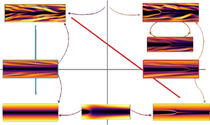
Figure 8. Sketch of the state space configuration. The four quadrants represent the basins of attraction corresponding to the states EIT, CAR, SAR, L. The solid lines emanating from the states represent trajectories approaching and departing different regions of the state space. The thick lines indicate the edge tracking carried out: between EIT and L (blue), between EIT and SAR (red) (see figure 9). The edge states resulting from the bisection algorithm are framed with the same colour. The chaotic attractors undergo calm and active phases (see figure 4) and approach the edge states during the calm phase.
The simplest edge state identified is the ‘lower branch’ unstable SAR between the ‘upper branch’ stable SAR and L (Buza et al. Reference Buza, Beneitez, Page and Kerswell2022a). Figure 9(a) shows the time series of the edge tracking between EIT and L and figure 9(c) shows a snapshot of this trajectory, a weakly chaotic state characterised by polymer layers located at  $y\approx \pm [0.75,0.85]$. The edge state reveals the significance of the polymer layers located close to the walls, as they are responsible for the self-sustained chaotic dynamics within the edge. Furthermore, these layers have been observed during the calm phases of both EIT and CAR, suggesting that they related to the driving mechanism for EIT. The edge state between CAR and L can be compared with the edge state found between EIT and SAR, figure 9(b,d), which also corresponds to a weakly chaotic state characterised by polymer layers located at $y\pm [0.75,0.85]$ with the presence of an arrowhead structure in the centre of the channel.

Figure 9. Top edge tracking for  $\textit {Re}=1000$, $\textit {Wi}=50$, $\beta =0.9$, $L_{{max}}=70$, $\textit {Sc}=500$: (a) between EIT and L (the green edge trajectory is bracketed by red trajectories approaching EIT and blue trajectories relaminarising to L), and (b) between EIT and SAR (the green edge trajectory is bracketed by red trajectories approaching CAR instead of EIT and blue trajectories approaching SAR). Bottom: (c) snapshot of tr $({\boldsymbol {C}})/{L_{{max}}^2}$ of the edge trajectory in (a) at $t=400$ that shows a strong polymer layer at $y\approx \pm [0.75,0.85]$. Plot (d) repeats this for (b). The red line in figure 8 explains how it is possible to reach the CAR edge state starting from a bisection between EIT and SAR.
The results of the edge tracking suggest an organisation of state space sketched in figure 8 over a two-dimensional plane of wall activity against centre-mode projection. Here each state is shown within its basin of attraction and the chaotic states are shown approaching their corresponding edge states in their calm phases. Our calculations suggest that there could be an intersection between the basins of attraction of EIT, CAR, SAR and L but the saddle state residing here is not computable using bisection since it must have two unstable directions.
4.2. Kinetic-to-elastic energy transfer
Our calculations of chaotic states highlight the importance of polymer activity at the walls. Here we identify the key location where kinetic energy is transferred to elastic polymer energy. The energy transfer flux from the perturbation kinetic energy to the perturbation elastic energy is
 \begin{equation} \varPi_e' := \frac{1-\beta}{\textit{Re}}T'_{ij}S'_{ij} \end{equation}
(e.g. see equations (9)–(12) in Dubief et al. Reference Dubief, Page, Kerswell, Terrapon and Steinberg2022), where primed variables indicate perturbations from the mean turbulent state, and the dissipation rate of TKE,  $\varepsilon :=({\beta }/{\textit {Re}})\partial _j u'_i\partial _j u'_i$, defines the Kolmogorov length scale,
 \begin{equation} \eta_K:=\left[\frac{(\beta/Re)^{3}}{\bar{\varepsilon}}\right]^{1/4}, \end{equation}
where  $\eta _K$ is defined for classic turbulence. Although $\eta _K$ might seem to depend on $\beta$ at first glance, the definition of $\textit {Re}$ is based on the total viscosity $\eta$.
Figure 10 shows the instantaneous cospectra of  $\varPi '_e$ and the corresponding instantaneous field of tr $(\boldsymbol {C})/L_{{max}}^2$ for each of EIT and CAR when they are on the verge of a high-activity phase. These cospectra highlight that as the trajectories depart from their calm phases, the largest rate of energy exchange from the kinetic energy to the elastic energy, i.e. maximal $\varPi _e'$, takes place at a location $y\approx [0.75,0.85]$ in (a) and $y\approx [-0.75,-0.85]$ in (b). Notably, the critical layer for the stable TS waves for $\textit {Re}=1000, \textit {Wi}=50,\ \beta =0.9,\ L_{{max}}=70,\ \textit {Sc}=500$ can be found at $y\approx \pm 0.79$. This corresponds to the location of the polymer layers harvesting kinetic energy to build self-sustained chaotic dynamics. The importance of the critical layer in supporting chaotic dynamics has been previously discussed in the transition route to EIT based on viscoelastic TS waves (Shekar et al. Reference Shekar, McMullen, Wang, McKeon and Graham2019, Reference Shekar, McMullen, McKeon and Graham2020, Reference Shekar, McMullen, McKeon and Graham2021). It is also interesting to note that the main exchange from elastic energy to kinetic energy happens in the dark regions of figure 10. As can be observed throughout the various figures in this work, this region supports the larger-scale motions during the observed self-sustained chaotic process. Moreover, these polymer sheets experience the same kind of undulation for the edge states as for the complex chaotic attractors when departing from the calm phases. The time-averaged cospectra (shown in figure 10e,f) confirm the importance of the energy exchange in the neighbourhood of the wall $y\approx [0.75,0.85]$. As expected, the time-averaged cospectra for EIT and CAR are very similar as the main energy exchange driving the chaotic dynamics is located in the same region (Dubief et al. Reference Dubief, Page, Kerswell, Terrapon and Steinberg2022).

Figure 10. (a) Cospectra between the perturbation kinetic energy to the perturbation elastic energy for EIT at  $\textit {Re}=1000,\ \textit {Wi}=50, \beta =0.9,\ L_{{max}}=70,\ \textit {Sc}=500$ as a function of the wall-normal coordinate $y$ just before an active phase. The streamwise wavenumber $k_x$ is normalised with the minimum mean Kolmogorov length scale. The white dashed line is at $y=0.75$. (c) Instantaneous snapshots of $\text {tr}(\boldsymbol {C})/L_{{max}}^2$ corresponding to the cospectra in (a). (b) Same as (a) but for snapshots of CAR at the same parameters. (d) Instantaneous snapshot of $\text {tr}(\boldsymbol {C})/L_{{max}}^2$ corresponding to the cospectra in (b). (e) Mean cospectra for same EIT as (a). (f) Idem for CAR in (b). The figure illustrates how the energy exchange ahead of an active phase occurs at polymer layers located at $y\approx \pm [0.75,0.85]$.
5. Discussion
In this paper we have carried out a suite of two-dimensional simulations of viscoelastic channel flow to explore where the various states described in Dubief et al. (Reference Dubief, Page, Kerswell, Terrapon and Steinberg2022) exist in  $(Wi,Re,\beta, L_{{max}},Sc)$ parameter space. A fully spectral code using the FENE-P model has been used to confirm the existence of four distinct states: the L state, SAR, CAR and EIT, EIT (the intermediate arrowhead state, IAR, of Dubief et al. (Reference Dubief, Page, Kerswell, Terrapon and Steinberg2022) has been clarified as a CAR where calm periods dominate over the chaotic dynamics). Elasto-inertial turbulence has been found for $(Wi,Re,\beta, L_{{max}},Sc) \in [30,100]\times [900,1200]\times [0.9,0.97]\times [50,130] \times [500,\infty )$ with increasing $Wi$,
$Wi$,  $Re$ and $\beta$ and decreasing $L_{{max}}$ intensifying the chaotic behaviour. Small $Sc$ values of $\approx 50$ suppress the chaotic dynamics, while larger values of $\textit {Sc}$ allow the chaos to exist in a greater region of parameter space.
The most significant finding, however, is that there is a substantial set of parameter values (shown in figure 2) where all four states coexist as attractors. This contrasts with the classic ‘supercritical’ scenario where a succession of unique attractors appear of increasing complexity as parameters are changed to make the flow more unstable (e.g. increasing  $Wi$ or decreasing $L_{{max}}$). In particular, no evidence has been found that a bifurcation off the SAR leads ultimately to either CAR or EIT (at least in two dimensions) as hypothesized after the recent discovery of the centre-mode instability (see, e.g. Garg et al. Reference Garg, Chaudhary, Khalid, Shankar and Subramanian2018; Page et al. Reference Page, Dubief and Kerswell2020; Khalid et al. Reference Khalid, Chaudhary, Garg, Shankar and Subramanian2021a; Datta et al. Reference Datta2022; Shankar & Subramanian Reference Shankar and Subramanian2022). It may well be that such a subcritical bifurcation sequence exists at, for example, higher $Wi$ or lower $L_{{max}}$ beyond the region of multistability. Our results do not go high enough in $Wi$ nor low enough in $L_{{max}}$ to see this. In terms of polymer concentration, SAR has been found as low as $\beta =0.5$ but remains stable even when chaotic dynamics emerges for $\beta \geq 0.9$.
To further probe the connection between the various states, various edge states were identified between pairs of attractors, and used to sketch the relative locations of the states in phase space. As expected, the edge state between SAR and L is the unstable ‘lower branch’ SAR found in Buza et al. (Reference Buza, Page and Kerswell2022b,Reference Buza, Beneitez, Page and Kerswella) while the edge states between CAR and L, and between EIT and SAR correspond to weakly chaotic states. The chaotic edge states reveal the presence of unstable polymer layers at  $y \approx \pm [0.75,0.85]$, qualitatively similar to the edge states between CAR and L, and between EIT and SAR. By examining the energy transfer flux, these near-wall polymer layers were found to be where the dominant energy transfer occurs from the velocity field to the polymers that seems fundamental for the self-sustained chaotic dynamics. In contrast, the chaotic flow appeared to be insensitive to the arrowhead structure populating the centreline region. This then further suggests that the chaotic dynamics is not related to the centre-mode instability or its arrowhead manifestation but is more a wall-focused phenomenon.
The conclusion of the present study is then that the two-dimensional linear instability discovered by Garg et al. (Reference Garg, Chaudhary, Khalid, Shankar and Subramanian2018) in pipe flow and Khalid et al. (Reference Khalid, Chaudhary, Garg, Shankar and Subramanian2021a) in a channel, and the resulting arrowhead structure (Page et al. Reference Page, Dubief and Kerswell2020; Buza et al. Reference Buza, Beneitez, Page and Kerswell2022a; Morozov Reference Morozov2022), appear dynamically disconnected from EIT at least in the two dimensions studied here. Instead, our study suggests that to trigger any chaotic motion, it is necessary to excite polymer layers located at  $y\approx \pm [0.75,0.85]$ from the wall. Recent work discussing viscoelastic TS waves (Shekar et al. Reference Shekar, McMullen, McKeon and Graham2020, Reference Shekar, McMullen, McKeon and Graham2021) suggests a plausible mechanism as polymer stretch is found localised at the near-wall critical layer of the TS waves. A three-dimensional route to EIT stemming from the arrowhead cannot be ruled out. Lellep et al. (Reference Lellep, Linkmann and Morozov2023) have shown that three-dimensional perturbations render the arrowhead linearly unstable and a possible route to EIT should be explored in this scenario. Another possibility is the very recent discovery of a wall-localised linear instability (Beneitez, Page & Kerswell Reference Beneitez, Page and Kerswell2023). Clearly, further efforts are needed to untangle the mechanism leading to EIT but now this can be focused on near-wall processes or three-dimensional alternatives.
Funding
The authors are grateful to EPSRC for supporting this work via grant EP/V027247/1. Y.D. also thanks the support of the National Science Foundation CBET (Chemical, Bioengineering, Environmental and Transport Systems) through award 1805636.
Declaration of interests
The authors report no conflict of interest.


 Open access