





1. Introduction
Subglacial drainage models have numerous uncertain parameters that control their behaviour (e.g. Werder and others, Reference Werder, Hewitt, Schoof and Flowers2013; Hager and others, Reference Hager, Hoffman, Price and Schroeder2022). If accurate subglacial drainage models are important in reproducing realistic ice-flow patterns as is often claimed (e.g. Khan and others, Reference Khan2024; Sommers and others, Reference Sommers2024), it follows that well-constrained model parameters are important for well-calibrated model predictions. Such predictions should have an associated uncertainty, and the predictive skill of any calibrated model should be critically assessed.
A common strategy used to select parameter values in a subglacial drainage model is to identify ‘low’, ‘medium’ and ‘high’ values for a subset of influential parameters (e.g. Dow, Reference Dow2022) and to sample these values with one-at-a-time (e.g. Khan and others, Reference Khan2024) or, rarely, all-at-once (e.g. Hager and others, Reference Hager, Hoffman, Price and Schroeder2022) sampling. In the absence of field data, parameter values may be selected based on producing a modelled drainage system consistent with prior expectations of realistic subglacial drainage (i.e. water pressure near ice overburden, seasonal development of subglacial channels) (e.g. Werder and others, Reference Werder, Hewitt, Schoof and Flowers2013). When data are available, models have been tuned based on consistency with radar specularity as a hypothesized indicator of channelized versus distributed flow (e.g. Dow and others, Reference Dow, McCormack, Young, Greenbaum, Roberts and Blankenship2020; Hager and others, Reference Hager, Hoffman, Price and Schroeder2022), satellite-altimetry-derived subglacial lake filling and drainage cycles (e.g. Wearing and others, Reference Wearing, Dow, Goldberg, Gourmelen, Hogg and Jakob2024) and mapped locations of eskers and other subglacial landforms indicative of past subglacial drainage characteristics (e.g. Hepburn and others, Reference Hepburn2024). Coupled hydrology–ice-flow models have also been tuned to match observed ice surface velocities (e.g. Ehrenfeucht and others, Reference Ehrenfeucht, Morlighem, Rignot, Dow and Mouginot2023; Khan and others, Reference Khan2024).
A suite of field data has been used in inverse models to infer more about subglacial drainage properties than revealed by manual tuning. Certain parameter values, such as the roughness of ice-walled englacial conduits which plays a role in heat transfer and conduit enlargement, have been inferred from experiments with tracer dye injections into moulins (e.g. Werder and Funk, Reference Werder and Funk2009) and moulin water-pressure measurements (e.g. Pohle and others, Reference Pohle, Werder, Gräff and Farinotti2022). However, given the expected discrepancy between modelled and observed subglacial drainage, the parameter values that describe the real system may not produce the best model–data fit. Inverse modelling approaches have constrained subglacial channel-network characteristics such as channel radius and hydraulic gradient based on dense passive seismic measurements (e.g. Nanni and others, Reference Nanni, Gimbert, Roux and Lecointre2021) or a combination of borehole water-pressure time series and tracer transit times (e.g. Irarrazaval and others, Reference Irarrazaval, Werder, Linde, Irving, Herman and Mariethoz2019, Reference Irarrazaval, Werder, Huss, Herman and Mariethoz2021). Based on a dense borehole array, Rada Giacaman and Schoof Reference Rada Giacaman and Schoof2023 characterized a spectrum of seasonal water-pressure patterns.
Formal model calibration and uncertainty quantification (e.g. Kennedy and O’Hagan, Reference Kennedy and O’Hagan2001; Higdon and others, Reference Higdon, Kennedy, Cavendish, Cafeo and Ryne2004), based on evaluating the misfit between model outputs and actual data over the entire space of plausible parameter values, provides a path forward for constraining the values of all influential model parameters and determining the corresponding best model predictions with associated uncertainty. Formal calibration of subglacial drainage model parameters has rarely been attempted. For instance, Irarrazaval and others (Reference Irarrazaval, Werder, Linde, Irving, Herman and Mariethoz2019, Reference Irarrazaval, Werder, Huss, Herman and Mariethoz2021) inferred the posterior distributions of channel network characteristics and hydraulic transmissivity by using a simplified, steady-state forward hydrology model to enable Bayesian inference. In the coupled hydrology–dynamics setting, calibration has been carried out by comparing modelled and satellite-derived annual average ice surface speed (Brinkerhoff and others, Reference Brinkerhoff, Aschwanden and Fahnestock2021).
In a previous study (Hill and others, Reference Hill, Bingham, Flowers and Hoffman2025), we constructed a Gaussian process emulator (e.g. Higdon and others, Reference Higdon, Gattiker, Williams and Rightley2008) of the Glacier Drainage System (GlaDS) subglacial drainage model (Werder and others, Reference Werder, Hewitt, Schoof and Flowers2013) that accelerates modelling by three orders of magnitude. In this study, we combine the Gaussian process emulator with borehole observations from western Greenland (Meierbachtol and others, Reference Meierbachtol, Harper and Humphrey2013; Wright and others, Reference Wright, Harper, Humphrey and Meierbachtol2016) to explore the possibility of more directly constraining subglacial drainage model parameters. Using Bayesian inference (e.g, Higdon and others, Reference Higdon, Kennedy, Cavendish, Cafeo and Ryne2004; Gelman and others, Reference Gelman, Carlin, Stern, Dunson, Vehtari and Rubin2013), we infer distributions of the eight most-uncertain GlaDS model parameters along with the corresponding uncertainty in calibrated model outputs. We first carry out a calibration experiment using a synthetic, model-generated water-pressure time series to quantify the performance and benefits of the emulator-based Bayesian calibration approach. Then, using real borehole water-pressure data, we derive calibrated, probabilistic estimates of parameter values and corresponding calibrated model predictions, and assess the remaining uncertainty and discrepancy in drainage-system characteristics to identify performance-limiting issues.
2. Real and synthetic water-pressure time series
The calibration experiments are carried out on a  $\sim 13\,000\,\mathrm{km}^2$ catchment in the Kangerlussuaq sector of western Greenland that includes Isunnguata Sermia (IS), Russell Glacier (RG) and Leverett Glacier (LG) basins (Fig. 1). This well-studied portion of the ice sheet has been used extensively for in situ and modelling studies of Greenland hydrology (e.g. Bartholomew and others, Reference Bartholomew, Nienow, Sole, Mair, Cowton, Palmer and Wadham2011; Sole and others, Reference Sole, Nienow, Bartholomew, Mair, Cowton, Tedstone and King2013; Lindbäck and others, Reference Lindbäck2015; Derkacheva and others, Reference Derkacheva, Gillet-Chaulet, Mouginot, Jager, Maier and Cook2021; Harper and others, Reference Harper, Meierbachtol, Humphrey, Saito and Stansberry2021), including previous emulator-based subglacial drainage modelling (Brinkerhoff and others, Reference Brinkerhoff, Aschwanden and Fahnestock2021; Verjans and Robel, Reference Verjans and Robel2024). Importantly, this sector of west Greenland has a suite of borehole time series data, including basal water pressure, obtained along a transect from near the margin up to 46 km inland spanning 2010–15 (see Table 1 from Wright and others, Reference Wright, Harper, Humphrey and Meierbachtol2016).
Greenland numerical domain and calibration data. (a) Study area within Greenland Ice Sheet. (b) Numerical mesh and flotation fraction for an example model output with approximate equilibrium line altitude sketched as dashed line (Smeets and others, Reference Smeets2018). (c) Example flotation fraction and channel discharge for the area below 1850 m a.s.l. with moulin positions from Yang and Smith Reference Yang and Smith2016 and location of in situ borehole water-pressure data (Meierbachtol and others, Reference Meierbachtol, Harper and Humphrey2013; Wright and others, Reference Wright, Harper, Humphrey and Meierbachtol2016) shown as a blue triangle. Atmospheric pressure (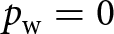 $p_\textrm{w}=0$) outlet nodes for Isunnguata Sermia (IS), Russell Glacier (RG) and Leverett Glacier (LG) are shown as red stars. (d) Ensemble of GlaDS-simulated flotation-fraction values and synthetic data. (e) Ensemble of GlaDS-simulated flotation-fraction values and in situ borehole data (Meierbachtol and others, Reference Meierbachtol, Harper and Humphrey2013; Wright and others, Reference Wright, Harper, Humphrey and Meierbachtol2016). Vertical dashed line in (d, e) corresponds to the day shown in (b, c).

2.1. Borehole water-pressure data
We use hydraulic head measurements from a drilling campaign described in Meierbachtol and others Reference Meierbachtol, Harper and Humphrey2013 and summarized by Wright and others Reference Wright, Harper, Humphrey and Meierbachtol2016. Over the 2010–15 period, a total of 32 boreholes were drilled to the bed, with 14 of these boreholes measuring basal water pressure. The majority of the boreholes where water pressure was measured were inferred to have intersected hydraulically isolated basal cavities (e.g. Meierbachtol and others, Reference Meierbachtol, Harper, Humphrey and Wright2016). Since the subglacial drainage model is a continuum model that assumes hydraulically connected drainage across the domain, we select a single water-pressure time series from a borehole ∼27 km from the margin (67.204∘ N, 49.718∘ W; Fig. 1c), denoted GL12-2A, as the only time series representing hydraulically connected drainage and that includes data from within and outside of the melt season (Fig. 1e). This borehole intersects a bed trough approximately 3 km across and 200 m deep, where the ice thickness is 695.5 m as measured with the drilling hose (Wright and others, Reference Wright, Harper, Humphrey and Meierbachtol2016). Hydraulic head values are converted into a fraction of overburden using the reported ice thickness and assuming an ice density  $\rho_\textrm{i} = 910\,\textrm{kg\,m}^{-3}$ (Wright and others, Reference Wright, Harper, Humphrey and Meierbachtol2016). The flotation fraction time series spans 16 June 2012 to 24 July 2013, and we use the data from the beginning of the record only until the end of 2012 for calibration since the data quality degrades the longer the instruments are deployed (personal communication from J. Harper, 2024). We compute the daily mean of the $\sim 15$-min data for comparison with model outputs.
2.2. Synthetic water-pressure data
We carry out a synthetic calibration experiment on the domain described above as a methodological example and to derive an upper bound on the strength of constraints that could be learned from point-scale water-pressure time series. Since there will be irreducible discrepancy between the model output and real borehole data, the real calibration experiment is expected to produce weaker constraints. The synthetic water-pressure data consist of modelled water pressure (as described in Section 3) using hidden parameter values, and the goal of the experiment is to assess the accuracy and uncertainty in inferred values. We use outputs chosen from a simulation that has high winter water pressure and low summer water pressure relative to the median simulation (Fig. 1d), since subglacial drainage models commonly underestimate winter water pressure relative to observations (e.g. Downs and others, Reference Downs, Johnson, Harper, Meierbachtol and Werder2018).
3. Forward model
3.1. Subglacial drainage model
We use the GlaDS model (Werder and others, Reference Werder, Hewitt, Schoof and Flowers2013) as the physically based forward model of subglacial drainage. GlaDS represents interacting distributed and channelized drainage systems. Distributed drainage is modelled as macroporous sheet flow and is intended to represent area-averaged flow through a network of hydraulically connected cavities formed in the lee of bed obstacles. Sheet flow transitions between laminar and turbulent regimes depending on the local Reynolds number (Hill and others, Reference Hill, Flowers, Hoffman, Bingham and Werder2024). Channelized drainage is modelled as a network of one-dimensional channels melted into the ice (Röthlisberger, Reference Röthlisberger1972), numerically located on the edges of mesh elements. The model does not represent hydraulically isolated or weakly connected drainage (e.g. Murray and Clarke, Reference Murray and Clarke1995; Andrews and others, Reference Andrews2014), which has been shown to play an important role in relating borehole water-pressure time series to surface-velocity observations (Hoffman and others, Reference Hoffman2016). We have therefore selected the borehole water-pressure record (as described above) that appears to best represent hydraulically connected drainage.
GlaDS requires specification of several poorly constrained parameters. We consider eight parameters,  $[k_\textrm{s}, k_\textrm{c}, h_\textrm{b}, r_\textrm{b}, A, l_\textrm{c}, \omega, e_\textrm{v}]$ (defined in Table 1), as the uncertain parameters to be calibrated. These parameters control the transmissivity of the drainage system ( $k_\textrm{s}$, $k_\textrm{c}$), the geometry of subglacial cavities ( $h_\textrm{b}$, $r_\textrm{b}$), the material rheology of the basal ice layer (A), the width of sheet flow that contributes to channelization ( $l_\textrm{c}$), the bulk Reynolds number at which sheet-flow transitions from laminar to turbulent (ω) and the englacial void fraction available for transient water storage ( $e_\textrm{v}$). One could in principle consider the channel-flow exponents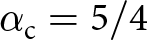 $\alpha_\textrm{c} = 5/4$ and $\beta_\textrm{c} = 3/2$ as uncertain calibration parameters as well. However, we assume flow in R-channels is well-described by turbulent Darcy–Weisbach flow $Q = - k_\textrm{c} S^{\alpha_\textrm{c}} \left| \frac{\partial \phi_\textrm{c}}{\partial x} \right|^{\beta_\textrm{c} - 2} \frac{\partial \phi_\textrm{c}}{\partial x}$ (Werder and others, Reference Werder, Hewitt, Schoof and Flowers2013) for discharge Q, channel area S, hydraulic potential ϕ and along-channel coordinate x and keep these parameters fixed. Other model parameters are physical constants, so we consider this to be a comprehensive assessment of parametric uncertainty, conditioned on the turbulent-channel assumption.
Constants (top group), fixed model parameters for GlaDS simulations (middle group) and model parameters and ranges used for training the Gaussian process emulator and inference (bottom group). The basal speed  $u_\textrm{b}$ and basal melt rate $\dot m_\textrm{s}$ are fixed, spatially varying fields, with bracketed values indicating the minimum and maximum

3.2. Model domain and discretization
The model domain is defined as a subglacial hydraulic catchment for the three proglacial outlets identified in Figure 1. These outlets correspond to the Isortoq River (for the IS sub-catchment) and two branches of the Sandflugtsdalen River (for the RG and LG sub-catchments) (fig. 1 from Lindbäck and others, Reference Lindbäck2015). The hydraulic catchment outline is defined by assuming water pressure is equal to ice overburden, 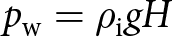 $p_\textrm{w} = \rho_\textrm{i} g H$, using 150 m-resolution IceBridge BedMachine Greenland (Morlighem and others, Reference Morlighem2017, Reference Morlighem2022) for surface elevation, bed elevation and the land–ice mask. The numerical domain consists of a triangular mesh with 4897 nodes that is refined to have edge lengths ∼500 m below 1000 m a.s.l. and as large as 5000 m above 2000 m a.s.l. (Fig. 1). For calibration and to generate synthetic data (Section 2.2), we extract modelled values at a single node near the borehole that was chosen to be most representative of observed conditions (Figs S1 and S2).
3.3. Melt and basal velocity forcing
We force GlaDS with daily surface melt and steady basal melt fields. Surface melt rates consist of daily mean 5.5 km-resolution RACMO2.3p2 (Noël and others, Reference Noël2018) surface runoff outputs for 2010–13. Meltwater is routed to the bed through 148 moulins previously mapped by Yang and Smith Reference Yang and Smith2016, with meltwater instantaneously accumulated within sub-catchments defined as Voronoi diagrams centred on each moulin. Basal melt rates are prescribed as the sum of melt rates from time-invariant geothermal and frictional heat fluxes. The geothermal flux linearly varies between  $27\,\textrm{mW}\,\textrm{m}^{-2}$ at the margin and $49\,\textrm{mW}\,\textrm{m}^{-2}$ at the ice divide based on borehole observations (Meierbachtol and others, Reference Meierbachtol, Harper, Johnson, Humphrey and Brinkerhoff2015). The frictional heat flux from sliding is computed as $u_\textrm{b} \tau_\textrm{b}$ for basal speed $u_\textrm{b}$ and basal drag τ b. We assume that basal speed $u_\textrm{b}$, basal drag and therefore frictional heat flux, are constant in time while acknowledging that substantial seasonal melt-forced velocity variations are observed in this region (e.g. van de Wal and others, Reference van de Wal2008; Derkacheva and others, Reference Derkacheva, Gillet-Chaulet, Mouginot, Jager, Maier and Cook2021). Basal drag is approximated as equal to the driving stress, $\tau_\textrm{b} = \rho_i g H |\nabla z_\textrm{s}|$, where $z_\textrm{s}$ is the surface elevation. Basal velocity is estimated as a uniform fraction of MEaSUREs multi-year (1995–2015) average surface velocities (Joughin and others, Reference Joughin, Smith, Howat and Scambos2016, Reference Joughin, Smith and Howat2018) by computing the ratio (0.33) that results in a maximum frictional-melt rate of $4\,\mathrm{cm\,w.e.\,a}^{-1}$ to match maximum frictional-melt rates derived from borehole data and satellite observations (Harper and others, Reference Harper, Meierbachtol, Humphrey, Saito and Stansberry2021).
We use daily average melt forcing and borehole water pressures, rather than resolving diurnal variations, to calibrate the drainage model because of the difficulty the model has in reproducing realistic diurnal variations and the challenge of constructing reasonably realistic sub-daily resolution melt inputs to drive the drainage model. When forced with diurnally varying melt inputs, GlaDS tends to produce muted variations over 24 hour periods, with larger variations on multi-day timescales (e.g. Hill and others, Reference Hill, Flowers, Hoffman, Bingham and Werder2024). This incorrect spectral response is opposite to that shown by the borehole time series, which has variations in the baseline water pressure on the order of 5% of overburden, with diurnal variations up to 15% of overburden. Perhaps because the model does not produce strong diurnal variations, the model predicts minimal differences in drainage system evolution between daily and sub-daily forcing (Werder and others, Reference Werder, Hewitt, Schoof and Flowers2013).
3.4. Boundary and initial conditions
No-flux subglacial drainage conditions are prescribed everywhere along the boundary, except at the three proglacial outlets where we prescribe zero water pressure. The outflow nodes are chosen as the nodes with locally minimum hydraulic potential, assuming water pressure equal to ice overburden, near the prescribed outlets used to define the hydraulic catchment (Fig. 1). We do not include an outflow node for the Point 660 catchment between the IS and RG catchments (Lindbäck and others, Reference Lindbäck2015) since we do not find a clear hydraulic potential minimum in this location. The model is initialized with no channels, water pressure equal to ice overburden and water layer thickness equal to 20% of the bed bump height. We run the model from 2010 until the end of 2012 and discard the first 2 years (2010–11) as a spin-up period to bring the model into a quasi-periodic state (e.g. Ehrenfeucht and others, Reference Ehrenfeucht, Morlighem, Rignot, Dow and Mouginot2023; Sommers and others, Reference Sommers2024).
3.5. Numerics
For the large ensemble of GlaDS simulations (Section 4.3), we have found that it is necessary to use a 0.2 h timestep and a solver residual tolerance of 10−5. This timestep is short compared to the daily melt-forcing frequency, and the 10−5 solver tolerance is smaller than often used for more typical GlaDS simulations. Using numerical parameters that are less strict results in noticeable changes in modelled water pressure for certain simulations in the ensemble (Fig. S16). Since we are purposely running GlaDS with unusual parameter values as part of the large ensemble, it is not unexpected that we need to be cautious in selecting numerical parameters to ensure that model runs are appropriately converged. We have also found that using simulations with numerical artefacts results in an emulator with high prediction error and parameter estimates that are inconsistent with the true parameter values in the synthetic calibration experiment since the simulation outputs do not change predictably with respect to model parameters. With these numerical parameters, each GlaDS simulation takes ∼8.75 hours on a single AMD Rome 7532 CPU and requires ∼1 GB of memory.
4. Inverse model
4.1. Bayesian inference
Given time series observations of subglacial water pressure, we aim to estimate the GlaDS parameter values that produce modelled water pressure consistent with the observations. Model–data fit is assessed by the sum-of-squares error between the observed time series and the modelled time series extracted at the node nearest to the borehole location. We use Bayesian inference to estimate probability distributions of GlaDS parameter values that minimize model–data squared error.
Let  $\boldsymbol{y} \in \mathbb{R}^{n_t}$ be the standardized observations, consisting of a number nt days of flotation fraction values. The observations y are standardized by subtracting the mean and dividing by the standard deviation of the simulation ensemble (Section 4.3). Consistent with previous work (e.g. Brinkerhoff and others, Reference Brinkerhoff, Aschwanden and Fahnestock2021), we apply a log-transform to the model parameters and standardize the log-parameters such that they fall in the interval $[0, 1]$. We denote the vector of log-standardized GlaDS parameters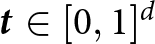 $\boldsymbol{t} \in [0, 1]^d$, where d = 8 is the number of calibration model parameters. With $F(\boldsymbol{t})$ the standardized (i.e. centred and scaled by the simulation mean and standard deviation) forward model (GlaDS) evaluated for log-standardized parameter values t, we model the observations as being generated from the forward model evaluated for some unknown calibration parameter values $\boldsymbol{t} = \boldsymbol{\theta}$,
 \begin{equation}
\boldsymbol{y} = F(\boldsymbol{\theta}) + \boldsymbol{\epsilon}_y.
\end{equation}
\begin{equation}
\boldsymbol{y} = F(\boldsymbol{\theta}) + \boldsymbol{\epsilon}_y.
\end{equation} The observation error 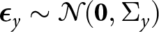 $\boldsymbol{\epsilon}_y \sim \mathcal{N}(\boldsymbol{0}, {\Sigma}_y)$ is modelled as multivariate normal with zero mean and covariance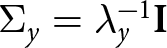 ${\Sigma}_y = \lambda_{y}^{-1} \mathbf{I}$ parameterized by precision λy. That is, we assume that the observations y are multivariate normally distributed with mean given by the standardized forward model evaluated for the unknown calibration parameters $F(\boldsymbol{\theta})$ and with covariance ${\Sigma}_y$: $\boldsymbol{y} \sim \mathcal{N}(F(\boldsymbol{\theta}), {\Sigma}_y)$.
From Bayes’ theorem, the distribution of the model parameters θ given the data, also called the posterior distribution, is
 \begin{equation}
P(\boldsymbol{\theta} | \boldsymbol{y}) \propto P(\boldsymbol{y} | \boldsymbol{\theta}) P(\boldsymbol{\theta}).
\end{equation}
\begin{equation}
P(\boldsymbol{\theta} | \boldsymbol{y}) \propto P(\boldsymbol{y} | \boldsymbol{\theta}) P(\boldsymbol{\theta}).
\end{equation} The first term on the right-hand-side,  $P(\boldsymbol{y} | \boldsymbol{\theta})$, called the likelihood, is the probability of sampling the data y from the model (1) given certain GlaDS parameters θ and represents model–data fit. For normally distributed errors, model–data fit is quantified by the squared error. The second term, $P(\boldsymbol{\theta})$, called the prior distribution, specifies our prior belief about the value of θ. Equation (2) indicates that we should update our belief in the calibration parameter values θ in light of the data y in order to reduce the squared error between the model and data. By maximizing the posterior probability (Eqn (2)), we minimize model–data misfit, with the prior distributions taking the place of regularization terms. As is common for Bayesian inference (e.g. Higdon and others, Reference Higdon, Kennedy, Cavendish, Cafeo and Ryne2004; Gelman and others, Reference Gelman, Carlin, Stern, Dunson, Vehtari and Rubin2013), we approximate the posterior distribution by iteratively sampling from the posterior distribution with Metropolis–Hastings Markov Chain Monte Carlo (MCMC; Metropolis and others, Reference Metropolis, Rosenbluth, Rosenbluth, Teller and Teller1953; Gattiker and others, Reference Gattiker, Klein, Hutchings and Lawrence2020). However, each likelihood evaluation $P(\boldsymbol{y}|\boldsymbol{\theta})$ involves running a forward GlaDS simulation. For the GlaDS model as used here, which takes ∼9 hours to run, sampling from the posterior (Eqn (2)) is intractable since the Metropolis–Hastings algorithm often requires thousands of sequential iterations to approximate the posterior distribution. To avoid this complication, we construct an emulator to stand in for GlaDS (e.g. Higdon and others, Reference Higdon, Kennedy, Cavendish, Cafeo and Ryne2004; Brinkerhoff and others, Reference Brinkerhoff, Aschwanden and Fahnestock2021).
4.2. Gaussian process emulator
Based on an ensemble of simulations with the forward model (GlaDS), the emulator estimates the simulated values for untested parameter values. We use a Gaussian process (GP) emulator that is more fully described by Hill and others Reference Hill, Bingham, Flowers and Hoffman2025. Instead of emulating the full spatiotemporal model outputs, here we emulate the flotation-fraction time series for the node representing the borehole. The GP requires additional parameters, which we call ‘hyperparameters’, whose values must be estimated (Table 2). We denote their calibration values ϕ to distinguish them from parameters of the subglacial drainage model (Table 1). Figure 2 and Algorithm S1 summarize the emulator-based calibration workflow.
Workflow for Gaussian process emulator-based calibration. t is the vector of log-standardized model parameters, with  $\boldsymbol{t} = \boldsymbol{\theta}$ the calibration parameters that best fit the data y, and $F(\boldsymbol{t})$ is the modelled time series of water pressure (expressed here as flotation fraction) corresponding to log-parameters t. The emulator η, with hyperparameters ϕ, is constructed as a linear combination of p principal component basis vectors kj and independent scalar emulators wj for $j=1, \ldots, p$. Uncertainty in the calibrated model is estimated by Monte Carlo sampling from the posterior parameter distribution.

Prior distributions on log-standardized subglacial drainage model parameters and Gaussian process hyperparameters. Uniform distributions  $U(a, b)$ are parameterized by the interval $[a, b]$. Gamma distributions $\Gamma(a, b)$ are parameterized by the shape parameter a and the rate parameter b such that the mean is $\frac{a}{b}$

Since GPs do not naturally scale to multivariate outputs such as a time series, we follow Higdon and others Reference Higdon, Gattiker, Williams and Rightley2008 in simplifying the problem using a principal component basis representation for the forward model outputs. Letting p denote the number of principal component basis vectors used in the representation, we model the standardized forward model output as
 \begin{equation}
F(\boldsymbol{t}) = \sum_{j=1}^p \boldsymbol{k}_j w_j(\boldsymbol{t}, \boldsymbol{\phi}) + \boldsymbol{\epsilon}_\eta,
\end{equation}
\begin{equation}
F(\boldsymbol{t}) = \sum_{j=1}^p \boldsymbol{k}_j w_j(\boldsymbol{t}, \boldsymbol{\phi}) + \boldsymbol{\epsilon}_\eta,
\end{equation} where kj ( $1 \leq j \leq p$) are the principal component basis vectors and wj ( $1 \leq j \leq p$) are independent GPs. For convenience, we refer to the first term as the emulator $\eta(\boldsymbol{t}, \boldsymbol{\phi}) = \sum_{j=1}^p \boldsymbol{k}_j w_j(\boldsymbol{t}, \boldsymbol{\phi})$. The error term $\boldsymbol{\epsilon}_\eta \sim \mathcal{N}(\boldsymbol{0}, \lambda_\eta^{-1}\mathbf{I})$, represents basis truncation error and is parameterized by the emulator precision λη. The number of principal components p that are retained is an important choice as it influences the fidelity of the emulator predictions. We will select the number of principal components for each application by considering the proportion of variance in the simulation ensemble that is explained, the truncation error and by inspecting the residuals in the basis representation. Full details of the consequences of the basis representation, including an expression for the likelihood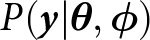 $P(\boldsymbol{y}|\boldsymbol{\theta}, \boldsymbol{\phi})$, are presented by Higdon and others Reference Higdon, Gattiker, Williams and Rightley2008.
Each individual GP wj is specified by its mean and covariance model. We use zero-mean GPs with a squared-exponential covariance function,
 \begin{equation}
k_j(\boldsymbol{t}, \boldsymbol{t}') = \frac{1}{\lambda_{w,j}} \exp\left(- \sum_{i=1}^d \beta_{ij} (t_{i} - t'_{i})^2 \right),
\end{equation}
\begin{equation}
k_j(\boldsymbol{t}, \boldsymbol{t}') = \frac{1}{\lambda_{w,j}} \exp\left(- \sum_{i=1}^d \beta_{ij} (t_{i} - t'_{i})^2 \right),
\end{equation} where  $\lambda_{w,j}$ is the marginal precision (inverse variance) of the GP wj and the βij ( $i=1, \ldots, d$) hyperparameters control the strength of dependence on each of the inputs. In practice, a small additional diagonal covariance matrix parameterized by precision λn (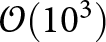 $\mathcal{O}(10^3)$), sometimes called a nugget, is added to each GP covariance matrix to improve the numerical conditioning of the matrix. The complete hyperparameter vector, accounting for the p separate values for the GP marginal precision $\boldsymbol{\lambda}_w$, input sensitivity β and nugget $\boldsymbol{\lambda}_n$, is $\boldsymbol{\phi} = [\lambda_y, \lambda_\eta, \boldsymbol{\lambda}_w, \boldsymbol{\beta}, \boldsymbol{\lambda}_n]$.
We sample from the joint posterior distribution,
 \begin{equation}
P(\boldsymbol{\theta}, \boldsymbol{\phi} | \boldsymbol{y}) \propto P(\boldsymbol{y} | \boldsymbol{\theta}, \boldsymbol{\phi}) P(\boldsymbol{\theta}) P(\boldsymbol{\phi}),
\end{equation}
\begin{equation}
P(\boldsymbol{\theta}, \boldsymbol{\phi} | \boldsymbol{y}) \propto P(\boldsymbol{y} | \boldsymbol{\theta}, \boldsymbol{\phi}) P(\boldsymbol{\theta}) P(\boldsymbol{\phi}),
\end{equation}which accounts for the uncertainty in the data y (Eqn (1)) as well as the replacement of the forward model with the GP emulator. We use the SEPIA package (Gattiker and others, Reference Gattiker, Klein, Hutchings and Lawrence2020) v1.1 to construct the emulators and carry out Metropolis–Hastings sampling. Choices for the prior distributions are discussed in Section 4.3. The foundation in uncertainty quantification is a primary benefit of GP modelling compared to other deterministic options for the emulator. In particular, the addition of the emulator uncertainty to the observation uncertainty in defining the GP likelihood (Higdon and others, Reference Higdon, Gattiker, Williams and Rightley2008) means that uncertainty in GP predictions is accounted for in inferring distributions of the model parameters. If the emulator has large uncertainty relative to the observational uncertainty, then the resulting posterior parameter distributions will be noticeably wider than had we used the forward model directly (e.g. Downs and others, Reference Downs, Brinkerhoff and Morlighem2023).
4.3. Ensemble design
We design the simulation ensemble to uniformly sample the log-standardized input space in order to construct an emulator with prediction performance that is approximately uniform across the log-inputs. For this, we use a Sobol’ sequence (Sobol’, Reference Sobol’1967) over the logarithm of the parameters within the bounds provided in Table 1. We draw 512 samples from the Sobol’ sequence, using its sequential design properties to evaluate emulator performance with power-of-2 subsets of the full sequence. We construct an independent set of inputs for testing the emulator consisting of 100 samples from a space-filling Latin hypercube design.
For parameters with a physical interpretation (e.g. the bed geometry as described by the bump height  $h_\textrm{b}$ and aspect ratio $r_\textrm{b}$, the ice-flow coefficient A and the laminar–turbulent transition parameter ω), we have chosen parameter ranges that encompass plausible values. For the remaining parameters, we have chosen their ranges to be reasonably wide while minimizing the number of unrealistic simulations, for example as indicated by water pressure exceeding 300% of overburden. We have found that this pressure constraint limits the lower bound of channel conductivity $k_\textrm{c}$, sheet conductivity $k_\textrm{s}$ and englacial storage parameter $e_\textrm{v}$.
These ranges largely encompass the values commonly used for modelling Greenland outlet glaciers with the GlaDS model (e.g. Gagliardini and Werder, Reference Gagliardini and Werder2018; Cook and others, Reference Cook, Christoffersen, Todd, Slater and Chauché2020; Ehrenfeucht and others, Reference Ehrenfeucht, Morlighem, Rignot, Dow and Mouginot2023; Khan and others, Reference Khan2024; Verjans and Robel, Reference Verjans and Robel2024; Hill and others, Reference Hill, Flowers, Hoffman, Bingham and Werder2024). Some exceptions include literature values of the englacial storage parameter as low as  $e_\textrm{v} =10^{-5}$ (e.g. Ehrenfeucht and others, Reference Ehrenfeucht, Morlighem, Rignot, Dow and Mouginot2023; Khan and others, Reference Khan2024), channel conductivity as low as $k_\textrm{c} = 0.05\,\textrm{m}^{3/2}\,\textrm{s}^{-1}$ (e.g. Khan and others, Reference Khan2024) and an ice-flow coefficient $A=2.5\times 10^{-25}\,\textrm{Pa}^{-3}\textrm{s}^{-1}$ indicative of basal ice below the pressure-melting point (Ehrenfeucht and others, Reference Ehrenfeucht, Morlighem, Rignot, Dow and Mouginot2023). Considering the laminar–turbulent sheet-flow model, it is difficult to compare the sheet conductivity range except for studies using a laminar sheet-flow model. Gagliardini and Werder Reference Gagliardini and Werder2018 and Cook and others Reference Cook, Christoffersen, Todd, Slater and Chauché2020 use a lower sheet conductivity value $k_{\textrm{s}}\approx 2 \times 10^{-4}\,\textrm{Pa}\,\textrm{s}^{-1}$, which we have found results in peak water pressures exceeding 300% of overburden for our setup.
4.4. Prior distributions
The prior distributions of GlaDS parameters  $P(\boldsymbol{\theta})$ and GP hyperparameters $P(\boldsymbol{\phi})$ in Eqn (5) are used to express our belief in the values of these quantities. For model parameters θ, we take a uniform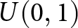 $U(0, 1)$ prior distribution for the log-standardized values to express a lack of prior belief in the most likely parameter values. We use Gamma distributions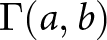 $\Gamma(a, b)$, parameterized by shape parameter a and rate parameter b, for the hyperparameter prior distributions $P(\boldsymbol{\phi})$ (Table 2) due to the flexibility of the Γ family of distributions and the fact that the probability density goes to 0 when $\boldsymbol{\phi}=0$. Since the inputs are scaled to the range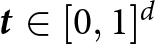 $\boldsymbol{t} \in [0, 1]^d$ and the outputs are centred and scaled to have unit variance, we select prior distributions for the observation precision λy, GP precision $\boldsymbol{\lambda}_\eta$ and GP sensitivity β that encourage values near 1. The GP nugget $\boldsymbol{\lambda}_n$ prior distribution encourages high precision (i.e. a small nugget) with a mean of 1000 and 95% interval spanning approximately an order of magnitude. We choose the prior distribution for the simulation precision λη to express our belief that this term should account for error in the truncated principal component basis. We choose the hyperparameters $a=a_\eta$ and $b=b_\eta$ to express this belief by constraining the mode to be equal to the precision of the basis representation, denoted λ p. We have found that prescribing a prior distribution that allows a wide range of simulation-precision values can sometimes result in the simulation error term ϵη absorbing all of the variations in the output with respect to θ, leaving the GP to revert to the mean irrespective of the given values of θ. To express our belief that the GP should take up variations in the simulator response for different parameter values, and therefore that λη represents the basis truncation error, we place 95% of the probability mass of the simulation-precision prior distribution within an interval with width equal to half of the basis precision λ p. For the truncation error in synthetic and borehole calibration experiments, the prior distribution parameter values are approximately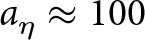 $a_\eta \approx 100$ and $b_\eta \approx 2$.
4.5. Posterior predictions
We produce calibrated GlaDS predictions by drawing 256 samples from the MCMC chain of GlaDS parameters (labelled  $\boldsymbol{\theta}_\textrm{post}$ in Fig. 2) and running the forward model (GlaDS) on the samples. Using GlaDS instead of the emulator to produce calibrated predictions allows us to investigate additional outputs such as the full spatiotemporal flotation fraction field and the distribution and extent of subglacial channels that are not predicted by the emulator.
5. Results
5.1. Emulator performance
The performance of the emulator is evaluated by computing the root-mean-square error (RMSE) between the flotation fraction of the test GlaDS runs extracted at the borehole location and the corresponding emulator predictions. The RMSE of the emulator is relatively consistent for different choices of the number of principal components and the number of simulations in the ensemble used to train the emulator (Fig. S4), with median time-integrated RMSE between 0.064–0.088 (in units of fraction of overburden). The RMSE decreases when increasing the number of principal components from 5 to 10, with minimal change for models with more principal components. Emulator performance improves for larger training ensembles, but with differences in the median performance remaining within the interquartile range. In other words, GP performance can be slightly improved by including more training simulations and principal components, but the error reduction is small compared to the variation in emulator error across the test set. The relatively weak sensitivity to the number of principal components and training simulations reported here is consistent with the more in-depth analysis carried out by Hill and others Reference Hill, Bingham, Flowers and Hoffman2025 for a simpler synthetic application. We choose to use the full set of 512 training simulations and 15 principal components, based on the levelling off of the emulator RMSE and the principal component truncation error (Fig. S3). In this case, the first 15 principal components explain 98% of the variation of the 512-member simulation ensemble.
The accuracy of the chosen emulator varies throughout the year and across the test set. To evaluate best- and worst-case scenarios for the emulator performance, we evaluate the 5th, 50th and 95th percentile realizations (Fig. 3). Absolute emulator prediction error is highest in the spring (days ∼150–175) and for simulations with high peak water pressure (e.g. Fig. 3a). After day ∼175, emulator predictions capture the amplitude and duration of water-pressure variations with lower absolute error. The relative emulator error is more consistent through the year, and for some test simulations is as large through late summer as during the spring pressure peak. Winter water pressure is reproduced within a few per cent of overburden. Correspondingly, emulator predictions are most uncertain, as measured by the width of the 68% and 95% prediction intervals, between days 150–175, with uncertainty reducing to a small fraction of overburden by winter. The 95% emulator prediction intervals mostly overlap the simulated values, except in spring (Fig. 3a), indicating the emulator is appropriately estimating prediction uncertainty.
Evaluation of the Gaussian process emulator. Comparison of GlaDS simulations and emulator predictions on the test set for individual simulations with high (95th-percentile, a), median (median, b) and low (5th-percentile, c) root-mean-square-error (RMSE).

5.2. Synthetic calibration experiment
For the synthetic calibration experiment, which aims to recover the true but hidden parameter values used for a reference GlaDS simulation that is labelled as data, emulator-based inference recovers the true parameter values within one standard deviation of the posterior distributions except for the sheet-channel width parameter  $l_\textrm{c}$ (Figs. 4 and S13). For all parameters except the laminar–turbulent transition parameter ω, the marginal posterior distributions (diagonal panels in Fig. 4) are more informative than the prior distributions. The posterior estimates of the channel conductivity $k_\textrm{c}$, ice-flow coefficient A and the englacial storage parameter $e_\textrm{v}$ are especially well-constrained relative to their prior distributions. We have found moderate pairwise correlations, including r = 0.48 between sheet conductivity $k_\textrm{s}$ and the bed bump aspect ratio $r_\textrm{b}$, and r = 0.48 between $k_\textrm{c}$ and A. The relatively weaker constraints on remaining parameters are consistent with a previous analysis of the sensitivity of flotation fraction to these parameters (Hill and others, Reference Hill, Bingham, Flowers and Hoffman2025). For ω, the lack of sensitivity may indicate that modelled sheet-flow at the borehole location remains laminar since this area tends to become channelized early in the melt season (Hill and others, Reference Hill, Flowers, Hoffman, Bingham and Werder2024)
Posterior distributions 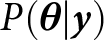 $P(\boldsymbol{\theta}|\boldsymbol{y})$ using synthetic water-pressure data. Diagonal panels show marginal prior and posterior distributions along with the hidden parameter values used to generate the synthetic data. Lower left panels show pairwise joint posterior distributions and values used to generate the data as crosses. Upper right panels show the estimated pairwise Pearson correlation coefficient.

Repeating the calibration experiment by individually considering each of the 100 test simulations as data, we consistently infer strong constraints on the value of the channel conductivity  $k_\textrm{c}$, ice-flow coefficient A, englacial storage parameter $e_\textrm{v}$ and the bed bump aspect ratio $r_\textrm{b}$ (Fig. S14) with very little bias (Fig. S15). While we typically constrain the sheet conductivity $k_\textrm{s}$, bed bump height $h_\textrm{b}$ and sheet-channel width $l_\textrm{c}$ values relative to their prior distributions, the true values are more likely to be in a lower posterior probability region (Table S1).
Calibrated model predictions have a 95% prediction interval that is 3.8 times narrower than that of the ensemble of simulations with parameter values sampled from the uniform priors (Fig. 5). As expected with synthetic data produced by the model, the calibrated predictions always overlap the synthetic data within the 95% prediction interval and often within the 68% interval (i.e. approximately within one standard deviation of the mean). While flotation fraction values between days ∼150–200 have been constrained relative to the prior distribution, there remains a spread of ∼100% of overburden in the 95% prediction intervals. However, this has been reduced from a spread of >200% of overburden in the original ensemble. The main discrepancy between the calibrated mean and the synthetic data is during the late-season melt events near day 250. Perhaps as a result of the biased posterior modes, the calibrated model has a faster flotation-fraction decay between these melt events than in the synthetic data.
Comparison of prior and calibrated ensembles of GlaDS simulations using the synthetic flotation-fraction time series. The mean and prediction intervals of the calibrated model are computed by running GlaDS with 256 samples from the posterior distribution.

5.3. Borehole calibration experiment
For the borehole data that covers the last 199 days (16 June to 31 December) of 2012, we choose to emulate only the corresponding period of modelled water pressure, rather than modelling the entire year as was done in the synthetic calibration experiment. This simplification allows us to reduce the number of principal components used by the emulator from 15 to 12 while still explaining 98% of the variance of the ensemble. We continue to use the full ensemble of 512 simulations to train the emulator.
5.3.1. Full time series calibration
As expected, calibration using the borehole water-pressure time series from 16 June to 31 December 2012 produces wider posterior distributions than the synthetic experiment (Fig. 6). Since we use the same prior distributions and GlaDS ensemble as in the synthetic experiment, these differences reflect how informative the real observations are compared to the synthetic observations. As we found in the synthetic calibration experiment, we obtain some constraint relative to the prior distribution on each parameter except the laminar–turbulent transition parameter ω. We obtain especially distinct posterior modes for channel conductivity  $k_\textrm{c}$, the bed bump aspect ratio $r_\textrm{b}$ and the ice-flow coefficient A. The bed bump height $h_\textrm{b}$, sheet–channel width $l_\textrm{c}$ and englacial storage parameter $e_\textrm{v}$ have indistinct modes but with a preference towards one side of their ranges. While we do resolve a posterior mode for the sheet conductivity $k_\textrm{s}$, this peak is not consistently observed for all emulator architectures (i.e. p values, Fig. S11) or when using different subsets of the simulation ensemble (Fig. S12), so we do not consider this a robust estimate. There is a moderate inverse correlation ( $r=-0.43$) between $k_\textrm{c}$ and $l_\textrm{c}$, with weaker correlations between other pairs. Compared to the synthetic experiment, even for parameters with a clear posterior mode (e.g. $k_\textrm{c}$ and $r_\textrm{b}$), the probability is nonzero across most of the range of values when using borehole data. The major exception is the ice-flow coefficient A, which has nearly zero marginal probability over most of its range except for the extreme upper end, indicating that the model is inconsistent with the borehole data for all but the highest A values (Section 6.1).
Posterior distributions  $P(\boldsymbol{\theta}|\boldsymbol{y})$ using borehole flotation-fraction data. Diagonal panels show marginal prior and posterior distributions. Lower left panels show pairwise joint posterior distributions. Upper right panels show the estimated pairwise Pearson correlation coefficient.

Calibrated model predictions (Fig. 7) highlight that, while the calibrated model sometimes aligns with the borehole time series, significant discrepancy remains between the calibrated model and the borehole time series. For instance, the coefficient of determination (the proportion of variance in the data explained by the calibrated model) is −3.2, where the negative indicates that the mean borehole flotation fraction is a better predictor than the calibrated model. For reference, the calibrated model predicts 93% of the variance in the synthetic calibration experiment. The negative coefficient of determination is a result of differences in the response to melt input variations between the calibrated model and the observations. In part, the model–data discrepancy may be a result of the borehole time series indicating a switch from connected to unconnected on day ∼215 of 2012. For the whole duration of the record, the model consistently responds more strongly to increases in melt rate than the borehole water-pressure time series, rapidly increasing water pressure by 5% to >10% of overburden. For various instances, the borehole water-pressure time series shows negligible pressure variations (e.g. after day 250) or out-of-phase variations (e.g. near day 175) relative to the calibrated model. Following day ∼220, the observed baseline water pressure increases by ∼5% of overburden. This increase is not reproduced by the model for any parameter combinations, as evidenced by the intermittent lack of overlap of the model 95% prediction intervals with the observations. The borehole record unfortunately does not cover the spring speedup event associated with high modelled water pressures. The calibrated model, which is therefore relatively unconstrained in the spring, predicts unrealistically high water pressure from days ∼150–165, with the mean prediction exceeding 150% of overburden and the 95% prediction interval reaching nearly 250%.
Comparison of prior and calibrated ensembles of GlaDS simulations using the real borehole flotation-fraction time series. The mean and prediction intervals of the calibrated model are computed by running GlaDS with 256 samples from the posterior distribution. The dashed box in (a) indicates the area shown in more detail in (b).

5.3.2. Independent summer and winter calibration
A major shortcoming of GlaDS and other similar models is that they typically produce low winter and high summer water pressures relative to measured or inferred water-pressure variations. This problem, in particular unrealistically high spring water pressure, persists in the calibrated model predictions. As one approach to improve the balance of winter and summer water pressure, Downs and others Reference Downs, Johnson, Harper, Meierbachtol and Werder2018 proposed using separate values for the sheet conductivity  $k_\textrm{s}$ within and outside of the melt season. To assess the extent to which we might infer distinct parameter values for these time periods, we separately calibrate the model using subsets of the borehole time series taken within and outside of the melt season. We use within melt season data between day 166 (the beginning of the record) until day 216, when the amplitude of diurnal variations suddenly decreases (not shown), suggesting the borehole may have lost full hydraulic connectivity. Since modelled and observed flotation fraction is nearly constant through winter, the principal component decomposition does not add value in terms of describing flotation-fraction patterns (i.e. the first principal component explains $\gg99\%$ of the variance), and so we define the (scalar) winter flotation fraction as the average over the last 30 days of the year.
By using different subsets of the borehole time series, we infer distinct posterior modes with overlapping distributions for the channel conductivity  $k_\textrm{c}$, bed bump aspect ratio $r_\textrm{b}$ and englacial storage parameter $e_\textrm{v}$ (Fig. 8). High values of the ice-flow coefficient A are preferred in all cases, but this preference is significantly weaker when using summer-only data. For the sheet conductivity $k_\textrm{s}$, the strongest posterior constraint is obtained by using the full time series. We do not find differences in the most-likely sheet conductivity values by separately using winter and summer data for calibration, despite the fact that the Downs and others Reference Downs, Johnson, Harper, Meierbachtol and Werder2018 sheet conductivity parameterization motivated this experiment. The distinct posterior parameter estimates for $k_\textrm{c}$ and $r_\textrm{b}$ act to increase winter water pressure and reduce summer pressure, consistent with the purpose but not the form of the sheet conductivity parameterization developed by Downs and others Reference Downs, Johnson, Harper, Meierbachtol and Werder2018. The englacial storage parameter $e_\textrm{v}$, which displays posterior modes at opposite extremes of its range using winter-only data compared to summer-only and all data, does not obviously fit this pattern. The preferentially high values using summer-only and all data may be a result of the model reducing the amplitude of the pressure response to surface melt events. While we have obtained some differences in estimated parameter values by using different subsets of the borehole data, we did not find a clear and useful pattern that supports seasonally changing GlaDS parameter values.
Comparison of marginal posterior parameter distributions using all borehole data or separately using summer and winter data.

5.4. Posterior constraints on subglacial drainage system
In both synthetic and borehole experiments, the single point-scale time series reduces model uncertainty everywhere in the domain (Fig. 9). More uncertainty remains in the borehole calibration experiment, consistent with the wider spread in spring flotation-fraction predictions at the borehole location (Figs. 5 and 7). In the synthetic calibration experiment, we have approximately halved the uncertainty in the total volume of the channel network relative to the spread of the original ensemble, with a posterior distribution consistent with the volume corresponding to the synthetic observation (Fig. 9d). In contrast, the borehole time series does not strongly constrain the volume of the channel network, but it does result in a preference towards larger channel networks than the original ensemble (Fig. 9e).
Calibrated drainage system characteristics and uncertainty. (a–c) Melt season-averaged flotation-fraction ensemble spread as measured by the width of the 95% prediction intervals before calibration (a), after calibrating with synthetic observations (b) and after calibrating with borehole observations (c). (d–e) Prior and calibrated domain-integrated channel volume on day 229 (16 August) corresponding to synthetic (d) and borehole (e) observations. The true channel volume in (d) corresponds to the simulation used as synthetic observations.

While the uncertainty in drainage system characteristics that remains after calibration with the borehole time series is larger than in the case of synthetic data, we do obtain meaningful constraints on channel network development throughout the domain and especially near the borehole location. Consistent with the channel network statistics (Fig. 9e), the model calibrated with the borehole time series shows, on average, higher channel discharge throughout the domain and especially within the IS sub-catchment (Fig. 10, see Fig. 1c for sub-catchment labels). Near the borehole, the calibrated model preferentially routes channelized flow along a consistent pathway that passes through the node used to represent the borehole. The calibrated model also has reduced flow through tributary branches which join below the borehole. Based on the difference in mean channel discharge, the borehole time series appears to provide some constraint on hydraulic potential gradients not only near the borehole but across the entire catchment.
Posterior channel network constraints. Mean channel discharge (using a minimum channel threshold  $Q \geq 2\,\textrm{m}^3\,\textrm{s}^{-1}$) on day 229 (16 August) for the area below 1850 m (left column) and near the borehole (right column) from the prior ensemble (top row) and after calibrating with borehole observations (bottom row). Mean flotation fraction for the corresponding ensembles is shown for context.

5.5. Computational savings
The emulator accelerates MCMC sampling by ∼5000 times (Table 3). This sampling density is not possible using GlaDS directly. Each GlaDS simulation takes ∼9 hours, and since we have used 5000 MCMC samples, drawing this many MCMC samples would take ∼5 years since MCMC demands sequential evaluation. Using the GP emulator with 512 simulations and 12–15 PCs, drawing the MCMC samples takes ∼6.5–8 hours. While more efficient sampling strategies are available that would require fewer samples, e.g. Metropolis-adjusted Langevin algorithm (Besag, Reference Besag1994; Roberts and Tweedie, Reference Roberts and Tweedie1996) or No-U Turn Sampling (Hoffman and Gelman, Reference Hoffman and Gelman2014), emulator-based sampling will provide denser samples and more fully resolved posterior distributions than using GlaDS directly for any of these sampling strategies. While it seems that some of the bias in posterior modes (e.g. Figs. 4, S14 and S15) may be partly a result of emulator error, this bias seems to be an appropriate trade-off for such a significant speedup in sampling.
Computation time corresponding to each step in the study. Computations were timed on AMD Rome 7532 CPUs on the Digital Research Alliance of Canada Narval cluster

6. Discussion
6.1. Parameter estimates
The synthetic calibration experiment shows that, even with perfect model–data fit, we do not learn about the true value of all parameters. This limitation arises in part because various parameter combinations produce similar outputs, as evidenced by the pairwise correlations up to  $|r| \geq 0.4$), and also because the point-scale flotation fraction is not sensitive to all parameters (e.g. Hill and others, Reference Hill, Bingham, Flowers and Hoffman2025). The slight bias in the most-likely inferred values might be partially explained by differences between emulator predictions and GlaDS simulations, as evidenced by the reduction in bias associated with including more principal components (Fig. S9) and adding more GlaDS simulations (Fig. S10), both of which reduce emulator prediction error (Fig. S4).
The real borehole time series yields weaker parameter constraints than the synthetic experiment. This is to be expected given the shorter observation period, which does not include the spring event, and the serious model–data discrepancy (e.g. Fig. 7). Despite these limitations, the posterior parameter distributions can guide parameter selection to produce model outputs that are closer to reality than by using uncalibrated values. In the case of the ice-flow coefficient, the inferred value  $A \approx 10^{-22}\,\textrm{Pa}^{-3}\,\textrm{s}^{-1}$ is outside the range typically suggested for basal ice at the pressure-melting point (e.g. Cuffey and Paterson, Reference Cuffey and Paterson2010) and perhaps points to model shortcomings, limitations in the model setup or discrepancy in the assumed n = 3 stress exponent (e.g. Millstein and others, Reference Millstein, Minchew and Pegler2022; Schohn and others, Reference Schohn, Iverson, Zoet, Fowler and Morgan-Witts2025). Other basal characteristics such as the anticipated high water content of basal ice (e.g. macroscopic water content of 2.9–4.6% within temperate basal ice; Brown and others, Reference Brown, Harper and Humphrey2017), anisotropic viscosity of basal ice (e.g. Hofstede and others, Reference Hofstede2018) and entrained debris (e.g. Harper and others, Reference Harper, Humphrey, Meierbachtol, Graly and Fischer2017) may also contribute to this high A value. For example, Cohen Reference Cohen2000 inferred ice-flow coefficients for simple shear as high as $A = 1.5 \times 10^{-22}\,\textrm{Pa}^{-3}\,\textrm{s}^{-1}$ at Engabreen, Norway, explained as representing enhanced shear as a consequence of bed-parallel unbound water layers laminated between layers of clean and dirty ice. Combined with the influence of unknown, irregular cavity geometries on creep-closure rates (e.g. Helanow and others, Reference Helanow, Iverson, Woodard and Zoet2021), it is not clear where to set a reasonable upper bound for the creep-closure ice-flow coefficient.
Of the eight calibration parameters (Table 1), the sheet conductivity  $k_\textrm{s}$, describing the transmissivity of the drainage system as a whole, the form of bed bumps as described by their height $h_\textrm{b}$ and aspect ratio $r_\textrm{b}$, and the channel conductivity $k_\textrm{c}$ most directly describe physical aspects of the subglacial drainage system. Other parameters are necessary for the model but describe aspects of the englacial drainage system (englacial storage parameter $e_\textrm{v}$) or basal ice that could be inferred through other means (ice-flow coefficient A), could be constrained by fluid-flow physics (laminar-turbulent transition parameter ω), or are model-specific parameters with little physical interpretation (sheet-width below channels $l_\textrm{c}$). The strongest constraints on physical subglacial hydraulic processes, therefore, would come from calibrating parameters in the first group listed above; however, we have obtained the strongest constraint on the ice-flow coefficient A. While the channel conductivity perhaps includes some information about subglacial and englacial conduits (e.g. Pohle and others, Reference Pohle, Werder, Gräff and Farinotti2022), we do not robustly learn about the scale of cavities through $h_\textrm{b}$ or the transmissivity of the drainage system through $k_\textrm{s}$ (Figs. 6 and S14). We have learned about $k_\textrm{s}$ in the synthetic calibration experiment, suggesting that model–data discrepancy, and perhaps the lack of borehole data during the spring, limits our ability to estimate this parameter from the data. In neither case do we learn about the bed bump height $h_\textrm{b}$, which controls the maximum water depth in subglacial cavities, reinforcing that point-scale water pressure is not sensitive to $h_\textrm{b}$ (e.g. Hill and others, Reference Hill, Bingham, Flowers and Hoffman2025).
The posterior estimates that we have derived based on calibration with the real borehole water-pressure time series differ from those derived by Brinkerhoff and others Reference Brinkerhoff, Aschwanden and Fahnestock2021 based on calibrating parameters of a coupled hydrology–ice-flow model applied to the same region in western Greenland. With a slightly modified version of GlaDS as the hydrology model, Brinkerhoff and others Reference Brinkerhoff, Aschwanden and Fahnestock2021 used a neural network emulator to estimate parameter distributions that produce the best fit to satellite-derived annual-average surface velocities. Our study and Brinkerhoff and others Reference Brinkerhoff, Aschwanden and Fahnestock2021 both constrain the most likely channel conductivity  $k_\textrm{c}$, bed bump aspect ratio $r_\textrm{b}$, and to some extent, the englacial storage parameter $e_\textrm{v}$. We obtain overlapping estimates with Brinkerhoff and others Reference Brinkerhoff, Aschwanden and Fahnestock2021 for $r_\textrm{b}$ and $e_\textrm{v}$, while our range of inferred $k_\textrm{c}$ values is two to three orders of magnitude higher. In addition to the parameters that we are able to infer, Brinkerhoff and others Reference Brinkerhoff, Aschwanden and Fahnestock2021 constrain the value of the sheet conductivity $k_\textrm{s}$ and the bed bump height $h_\textrm{b}$. We obtain a strong constraint on the ice-flow coefficient A, which Brinkerhoff and others Reference Brinkerhoff, Aschwanden and Fahnestock2021 did not calibrate. These studies infer different pairwise correlations between subglacial drainage model parameters. Brinkerhoff and others Reference Brinkerhoff, Aschwanden and Fahnestock2021 find correlation $r=-0.79$ between $k_\textrm{s}$ and $h_\textrm{b}$, while we find a much weaker relationship ( $r=-0.24$). This difference may be a consequence of the different sheet-flow parameterizations or that the values of A that we infer are compensating for model shortcomings that are otherwise taken up by other parameters including $k_\textrm{s}$ and $h_\textrm{b}$. We find a correlation r = 0.31 between $r_\textrm{b}$ and $e_\textrm{v}$, whereas Brinkerhoff and others Reference Brinkerhoff, Aschwanden and Fahnestock2021 report a slightly lower correlation of r = 0.2.
The comparable or stronger parameter constraints obtained by Brinkerhoff and others Reference Brinkerhoff, Aschwanden and Fahnestock2021 suggest that this single borehole water-pressure time series does not contain more information to constrain the parameters of subglacial drainage models than annual-average surface velocities, despite the impact of the filtering effect of ice flow on estimates based on surface velocities. This conclusion hinges on the discrepancy of the subglacial drainage model compared to the borehole water pressure since we obtain much more informative distributions when we remove the discrepancy by using synthetic model-generated data for calibration (Fig. 4). It is also possible that we would more strongly constrain other parameter values, particularly for parameters correlated with A, if we did not vary A across the ensemble (cf. Brinkerhoff and others, Reference Brinkerhoff, Aschwanden and Fahnestock2021). Stronger constraints may also be obtained with multiple, multi-year borehole water-pressure records that cover the full melt season including the spring speedup and a model that more closely matches the measured time series (e.g. Andrews and others, Reference Andrews2014; Ryser and others, Reference Ryser2014; Hoffman and others, Reference Hoffman2016). With multiple multi-year borehole time series, it could also be worthwhile to repeat the separate summer–winter calibration experiment (Fig. 8) to reassess whether the results support seasonally varying parameter values (e.g. Downs and others, Reference Downs, Johnson, Harper, Meierbachtol and Werder2018). Combining both surface-velocity observations and borehole water-pressure data into a single calibration exercise could also provide stronger parameter estimates and further reduce prediction uncertainty.
6.2. Calibrated predictions and drainage-system characteristics
Using a single point-scale flotation-fraction time series, we have reduced the uncertainty in modelled flotation fraction and the configuration of subglacial channels by at least a factor of three in both synthetic and borehole experiments. Uncertainty reduction is appealing from a modelling perspective, however, it is concerning from the view of realistic subglacial drainage. Borehole records such as the one we have used to calibrate the model show pressure gradients as steep as  $10\,\textrm{kPa}\,\textrm{m}^{-1}$ between boreholes separated by tens of meters (e.g.
Ryser and others, Reference Ryser2014; Wright and others, Reference Wright, Harper, Humphrey and Meierbachtol2016) and hydraulic connectivity that varies over similar length scales (e.g. Wright and others, Reference Wright, Harper, Humphrey and Meierbachtol2016; Rada Giacaman and Schoof, Reference Rada Giacaman and Schoof2023). The lack of representation of this basal heterogeneity in models (cf. Hoffman and others, Reference Hoffman2016) results in unrealistically high confidence in inferred parameter values and calibrated predictions. The extent of overconfidence could be assessed by repeating the inference with multiple water-pressure time series from nearby boreholes that intersect hydraulically connected drainage if such data were available. For other model limitations, it is more challenging to assess how deficiencies in the theory underpinning models impacts uncertainty in the calibrated model (Section 6.4)
$10\,\textrm{kPa}\,\textrm{m}^{-1}$ between boreholes separated by tens of meters (e.g.
Ryser and others, Reference Ryser2014; Wright and others, Reference Wright, Harper, Humphrey and Meierbachtol2016) and hydraulic connectivity that varies over similar length scales (e.g. Wright and others, Reference Wright, Harper, Humphrey and Meierbachtol2016; Rada Giacaman and Schoof, Reference Rada Giacaman and Schoof2023). The lack of representation of this basal heterogeneity in models (cf. Hoffman and others, Reference Hoffman2016) results in unrealistically high confidence in inferred parameter values and calibrated predictions. The extent of overconfidence could be assessed by repeating the inference with multiple water-pressure time series from nearby boreholes that intersect hydraulically connected drainage if such data were available. For other model limitations, it is more challenging to assess how deficiencies in the theory underpinning models impacts uncertainty in the calibrated model (Section 6.4)
6.3. Modelling limitations and challenges
We have made numerous choices in setting up the subglacial drainage model, for instance forbidding cavities from opening by viscous creep, using the laminar–turbulent sheet-flow model (Hill and others, Reference Hill, Flowers, Hoffman, Bingham and Werder2024), and using satellite-mapped moulin positions rather than transferring surface melt directly to the bed at each node. It would be possible to include the effect of these choices in the calibration by encoding them as categorical variables. We have instead opted to use the most physically justified option in each case and infer the corresponding parameter values conditioned on the model configuration.
For cavity creep opening, we argue that disallowing opening by viscous creep is the more physically realistic choice because of the disparate timescales between slow creep-opening (days to weeks) and the timescale corresponding to subglacial overpressurization (hours to days) along with the associated unmodelled processes (e.g. hydrofracture, Das and others, Reference Das, Joughin, Behn, Howat, King, Lizarralde and Bhatia2008; Tsai and Rice, Reference Tsai and Rice2010). Furthermore, allowing cavity creep-opening results in extensive regions (e.g. tens of kilometres inland along bed troughs) with sheet thicknesses exceeding the bed bump height for much of the melt season and effectively forming a subglacial lake. We have used the most realistic meltwater inputs reasonably possible at daily resolution, using moulins mapped from Landsat imagery (Yang and Smith, Reference Yang and Smith2016) and surface runoff outputs from the RACMO2.3p2 model (Noël and others, Reference Noël2018). The laminar–turbulent sheet-flow model is consistent with the well-understood physics of potential gradient-driven flow and produces improved winter water pressures relative to a turbulent-only model (Hill and others, Reference Hill, Flowers, Hoffman, Bingham and Werder2024).
Based on sensitivity tests, modelled water pressure at the borehole location is sensitive to the above modelling choices (Fig. S17). Despite efforts to produce a realistic, data-informed model setup, using a simpler, less realistic model results in a better fit to the borehole data in the case of cavity creep-opening and the moulin configuration (Fig. S18), although the single borehole record used here does not provide enough data to assess these modelling choices more generally. For meltwater inputs through moulins, it is possible that we are missing additional moulins that are fed by streams that are too small to be resolved in the 15 m-resolution Landsat imagery (Yang and Smith, Reference Yang and Smith2016). If this is the case, then a denser moulin configuration may result in model outputs closer to those obtained by transferring surface melt to the bed at every node, while being more realistic. The paradox that using more data in the model setup and intentionally choosing, a priori, the most reasonable parameterizations degrades model performance highlights the challenge of modelling subglacial drainage with the current generation of models and input data. It remains possible that two-way coupling with an ice-flow model which captures hydrology–sliding feedbacks could improve model outputs by reducing the amplitude of pressure variations and increasing winter water pressure (e.g. Hoffman and Price, Reference Hoffman and Price2014).
The discrepancy in spatial footprints of the observations and the model makes it difficult to determine which node should be used as the most representative of the borehole observations. For the numerical mesh used here, there are three nodes similarly spaced within 386–454 m of the borehole (Fig. S1). We have chosen to use a node located in the centre of the trough that most consistently has a modelled subglacial channel passing through it (Fig. 10). Since water pressure sometimes varies between these three similarly distant nodes (Fig. S2), it would be best practice for future calibration studies to refine the model mesh around the location of any observations, consider forcing the mesh to have a node at the precise location of the borehole, and to evaluate the sensitivity of the calibration results to the node being used for calibration, considering the possibility of errors in bed elevation. Ideally, multiple borehole time series co-located within the same mesh element could be averaged to upscale the observations. However, the expense of drilling and the high likelihood of intersecting hydraulically isolated bed patches with any given borehole make it rare to find multiple co-located boreholes suitable for comparison with continuum models. Instead, complementary data such as proglacial discharge estimates tracer transit times and concentrations could be used in a multi-stage Bayesian calibration (e.g. Aschwanden and Brinkerhoff, Reference Aschwanden and Brinkerhoff2022) to provide additional constraints on the drainage model.
6.4. Perspectives on subglacial drainage models
The discrepancy between the subglacial drainage model and reality (Fig. 7), and the finding that model predictions are made worse by including more physical insight when making model choices and using real data in the model configuration (Figs S17 and S18), suggests that we should ask: is the subglacial drainage model a useful representation of borehole water pressure? From the perspective of model–data misfit, the model is less useful than simply averaging the observations to obtain a single mean value of water pressure over time. In other words, the model does not effectively reproduce observed variations in borehole water pressure for any parameter values that we have tested. This conclusion does not even consider the behaviour of the model in the spring, when modelled pressure exceeds 150% of overburden for at least several days over a large portion of the domain, violating basic vertical force balance. It does not appear that the model–data misfit will improve with additional data to constrain it, since the misfit appears to be at least partially related to fundamental model shortcomings, rather than arising from residual parameter uncertainty which could plausibly be reduced by additional measurements.
Should the goal of subglacial drainage modelling be to precisely match individual borehole water-pressure time series? Borehole observations characteristically exhibit variability in baseline water pressure and the response to melt forcing over spatial scales of tens of meters or less (e.g. Murray and Clarke, Reference Murray and Clarke1995; Ryser and others, Reference Ryser2014; Wright and others, Reference Wright, Harper, Humphrey and Meierbachtol2016). Considering that ice flow is sensitive to basal conditions averaged over scales of several ice thicknesses (e.g. Kamb and Echelmeyer, Reference Kamb and Echelmeyer1986), this does not seem like a productive goal for the purpose of explaining and predicting variations in sliding rates, which is the most common motivation for subglacial drainage model development. Instead, a more approachable goal would be to match the average features observed in multiple boreholes, intersecting both hydraulically isolated and connected drainage, within a spatial footprint of several ice-thicknesses.
These conclusions put modellers in a challenging position. It is well-understood that surface melt-forced variations in subglacial drainage influence glacier (e.g. Iken and Bindschadler, Reference Iken and Bindschadler1986) and ice-sheet dynamics (e.g.
Joughin and others, Reference Joughin, Das, King, Smith, Howat and Moon2008; Bartholomew and others, Reference Bartholomew, Nienow, Mair, Hubbard, King and Sole2010; Palmer and others, Reference Palmer, Shepherd, Nienow and Joughin2011). However, our application of a popular subglacial drainage model suggests that it cannot reasonably reproduce direct measurements of subglacial drainage, even when calibrated with real data and parametric uncertainties are accounted for. We suggest that a productive path forward is to re-examine the overall structure of subglacial hydrology models, for instance englacial storage, processes associated with pressures exceeding overburden (e.g. Tsai and Rice, Reference Tsai and Rice2010; Schoof and others, Reference Schoof, Hewitt and Werder2012), two-way hydrology–sliding feedbacks (e.g. Hoffman and Price, Reference Hoffman and Price2014), the form of the relationship between hydrology and basal friction (e.g. Gilbert and others, Reference Gilbert, Gimbert, Thøgersen, Schuler and Kääb2022) and heterogeneous hydraulic connectivity (Hoffman and others, Reference Hoffman2016), to improve model behaviour on appropriate spatial and temporal scales. Concurrently, ice-flow models could adopt effective-pressure parameterizations that are consistent with observed borehole water pressures, e.g. effective pressure  $N = 5\mbox{--}20\%$ of overburden (e.g. Wright and others, Reference Wright, Harper, Humphrey and Meierbachtol2016) until such subglacial drainage models are developed.
7. Conclusions
We have applied an emulator-based Bayesian calibration method to enable efficient Bayesian inference of parameters of the GlaDS subglacial hydrology model (Werder and others, Reference Werder, Hewitt, Schoof and Flowers2013) given time series observations of flotation fraction (i.e. water pressure relative to ice overburden) at daily resolution. Using borehole water-pressure data from western Greenland, we obtain meaningful constraints on the channel conductivity  $k_\textrm{c}$, bed bump height $r_\textrm{b}$, ice-flow coefficient A and englacial storage parameter $e_\textrm{v}$, with correspondingly reduced uncertainty in modelled water pressure. Relative to the uncalibrated model, we have constrained the configuration of subglacial channels near the borehole and, to a lesser degree, across the entire catchment.
The calibrated water-pressure time series overlaps with the overall range of water pressure observed in the borehole, but the calibrated predictions fail to match observed surface melt-forced water-pressure variations. We have shown that this discrepancy between modelled subglacial drainage and borehole observations is not a result of the choice of model parameters, but is rather a structural feature of the model and therefore is unlikely to be reduced by integrating additional field data. While it is unreasonable to expect a spatially distributed continuum model to precisely predict point-scale (i.e. borehole) water-pressure variations, the structural discrepancy suggests that the limitations of physics-based drainage models, rather than parameter uncertainty or their computational cost, are a rate-limiting step in predicting hydraulically-forced seasonal ice-flow variations.
Supplementary material
The supplementary material for this article can be found at https://doi.org/10.1017/aog.2025.10016.
Data availability statement
Code for running GlaDS experiments and calibrating the drainage model, GlaDS model outputs and MCMC samples are available at https://doi.org/10.5281/zenodo.15412093 (Hill and others, Reference Hill, Flowers, Bingham and Hoffman2025b). Surface elevation and ice thickness data are from https://doi.org/10.5067/GMEVBWFLWA7X (Morlighem and others, Reference Morlighem2022). The SEPIA package v1.1 (Gattiker and others, Reference Gattiker, Klein, Hutchings and Lawrence2020), used for emulator-based Bayesian inference, is available at https://github.com/lanl/SEPIA/. The Ice-sheet and Sea-level System Model (ISSM) used for GlaDS simulations is available at https://issm.jpl.nasa.gov/ (Larour and others, Reference Larour, Seroussi, Morlighem and Rignot2012). Borehole water-pressure data are available at https://doi.org/10.18739/A20C4SM8X (Harper and Humphrey, Reference Harper and Humphrey2010-2014). Daily surface runoff outputs from the 5.5 km-resolution RACMO2.3p2 model are available by contacting the Institute for Marine and Atmospheric Research Utrecht.
Acknowledgements
TH was supported by Simon Fraser University and the Natural Sciences and Engineering Research Council of Canada (NSERC) Canada Graduate Scholarship program. GF and DB received support from the NSERC Discovery Grants program. This material is based upon work supported by the U.S. Department of Energy, Office of Science, Office of Biological and Environment Research and Office of Advanced Scientific Computing Research under Triad National Security, LLC (‘Triad’) contract grant 89233218CNA000001 [FWP: LANLF2C2]. This research was enabled in part by support provided by WestDRI (https://training.westdri.ca), Calcul Quebec (https://www.calculquebec.ca/) and the Digital Research Alliance of Canada (https://alliancecan.ca). RACMO2.3p2 model outputs were kindly provided by Christiaan van Dalum. We would like to thank Joel Harper for helpful discussions and for providing borehole data, and Martin Lüthi and an anonymous reviewer for comments on an earlier version of this manuscript.
Author contributions
GF, TH and MH conceived of the idea of constraining subglacial drainage model parameters with water-pressure time series. TH and DB contributed to the emulator and calibration methodology with input from MH. TH, GF and MH constructed the subglacial drainage model setup. TH developed and ran the code and visualized the outputs. TH led the manuscript preparation with contributions from GF, DB and MH. All authors interpreted the calibration results and edited the manuscript.


 Open access

