2.1. Computational domain

The used computational domain is sketched in figure 2, with streamwise extent ${L_x=150{\delta _{in}}}$ (where $\delta _{in}$ is the inflow boundary layer thickness), spanwise length ${L_z}=60{\delta _{in}}$, domain height ${L_y}=30{\delta _{in}}$, and discretized with a grid including $1536 \times 384 \times 1280$ nodes. Uniform spacing is used in the streamwise and spanwise directions, whereas nodes are clustered in the wall-normal ($y$) direction up to $y/\delta _{in} = 6.5$. Streamwise and spanwise spacings are $\Delta x^+ \approx 10$ and $\Delta z^+ \approx 5$, respectively, whereas the spacing in the wall-normal direction ranges between $0.7$ at the wall and $12$. Here and elsewhere, the $+$ superscript is used to denote normalization with respect to the friction velocity $u_\tau = \sqrt {\tau _w/\rho _w}$ (where $\tau _w$ and $\rho _w$ are the wall shear stress and density), and the viscous length scale is $\delta _v = \nu _w / u_\tau$ (where $\nu _w$ is the wall kinematic viscosity). The domain and its discretization are the same as employed in our previous work (Zuo et al. Reference Zuo, Memmolo, Huang and Pirozzoli2019; Zuo, Yu & Pirozzoli Reference Zuo, Yu and Pirozzoli2022), where we show that it is sufficient to simulate the physics of the flow correctly.

Figure 2.

Sketch of computational domain for CSBLI analysis. Here, $\delta _{in}$ is the inflow boundary layer thickness, $x_{rec}$ is the boundary layer recycling station, and ${x_c}$ is the $x$ coordinate of the cone leading edge. The green surface depicts the conical shock, whose wall trace is highlighted in red.

2.2. Treatment of the shock generator

We rely on the immersed boundary method (Fadlun et al. Reference Fadlun, Verzicco, Orlandi and Mohd-Yusof2000) to accommodate the conical shock generator in the simulation. Solid and fluid nodes are located by means of a ray tracing algorithm (O'Rourke Reference O'Rourke1998). Interface nodes are fluid nodes whose stencil includes solid nodes, and on which flow parameters are imposed explicitly according to an equilibrium wall function (Tessicini et al. Reference Tessicini, Iaccarino, Fatica, Wang and Verzicco2002). Implementation details are provided in Bernardini, Modesti & Pirozzoli (Reference Bernardini, Modesti and Pirozzoli2016). The cone is resolved with approximately 72, 56 and 138 grid intervals in the streamwise, wall-normal and spanwise directions, respectively. As proven in Zuo et al. (Reference Zuo, Memmolo, Huang and Pirozzoli2019), although the boundary layer on the cone is certainly not well resolved, this is not a major shortcoming, as the cone serves simply as a disturbing element to force a spatially varying pressure gradient onto the underlying boundary layer.

2.3. Flow conditions

The flow conditions are selected to be as close as possible to the reference experiment of Hale (Reference Hale2015). The shock generator is a cone with height $L/\delta _{in}=6.835$ and half opening angle $\theta _c = 25^\circ$. The apex of the cone is at ${x_{c}} = 30{\delta _{in}}$ from the inflow, and its axis is parallel to the wall at a distance $h/ \delta _{in}=13.67$ (see figure 2). The upstream flow has Mach number $M_{\infty } = 2.05$, and the Reynolds number based on the inflow boundary layer thickness is $\textit {Re}_{\delta _{in}}=5000$. The latter is approximately a factor of fifty less than the reference experiment, but as shown in Zuo et al. (Reference Zuo, Memmolo, Huang and Pirozzoli2019), this is not the cause of major quantitative differences.

A realistic boundary layer is achieved through a rescaling–recycling procedure (Xu & Martin Reference Xu and Martin2004), whereby a cross-stream slice of the flow field is extracted at every Runge–Kutta sub-step at the recycling station $x_{rec}$, and fed back to the inflow upon suitable rescaling. To minimize spurious time periodicity that may result from application of quasi-periodic boundary conditions in the streamwise direction, the recycling station is set at $x_{rec} = 25 \delta _{in}$, also sufficiently upstream of the cone apex. Non-reflecting characteristic boundary conditions are applied to the outflow, at the top boundary, and in the spanwise direction for $x>x_{rec}$, whereas spanwise periodicity is assumed for $x \leq x_{rec}$. Unsteady characteristic boundary conditions are specified at the bottom no-slip wall (Poinsot & Lele Reference Poinsot and Lele1992), with temperature set to its adiabatic value. Flow statistics have been collected from time $t_0 u_\infty / \delta _{in} \approx 1711$ to time $t_f u_\infty / \delta _{in} \approx 3461$, at intervals of $\Delta t\,u_\infty / \delta _{in} \approx 0.1$. The long sampling time is needed to achieve convergence of pointwise statistics in time in the absence of homogeneous directions, and it makes the present calculation quite time-consuming. The statistical analysis is carried out by splitting the instantaneous quantities into their mean and fluctuating components, using either the standard Reynolds decomposition $f=\bar {f} + f'$, or the density-weighted (Favre) decomposition $f = \tilde {f} + f''$, where $\tilde {f} = \overline {\rho f} /\bar {\rho }$.

2.4. Assessment of flow properties

A necessary check is that the incoming boundary layer is developed properly prior to interaction with the conical shock. For that purpose, we consider a reference station at $x_{ref} = 27.5 \delta _{in}$, located upstream of the cone leading edge. The global boundary layer properties at this station are listed in table 1, where $\delta$ is the $99\,\%$ thickness, $\delta ^*$ is the displacement thickness,

(2.1)\begin{equation} \delta^* = \int_0^{{\delta_e}} \left( 1 - \frac{{\bar{\rho}}}{{{\rho_e}}}\,\frac{{\bar{u}} }{{{u_e}}} \right) {\mathrm d} y , \end{equation}

and $\theta$ is the momentum thickness,

(2.2)\begin{equation} \theta = \int_0^{{\delta_e}} \frac{{\bar{\rho}}}{{{\rho_e}}}v\frac{{\bar{u}}}{{{u_e}}}\left( {1 - \frac{{\bar{u}}}{{{u_e}}}} \right) {\mathrm d} y , \end{equation}

with the upper integration limit $\delta _e$ denoting the edge of the rotational part of the boundary layer, defined as the point where the mean spanwise vorticity becomes less than $0.005{u_\infty }/{\delta _{in}}$ (Pirozzoli et al. Reference Pirozzoli, Bernardini and Grasso2010). The subscript $e$ is used to denote the corresponding external flow properties.

Table 1.

Boundary layer properties at selected streamwise stations for pressure field analysis. Subscripts: $e$ indicates properties at the edge of the boundary layer; $w$ indicates wall properties; and $\infty$ indicates free-stream properties. Here, $\textit {Re}_\theta = \rho _e u_e \theta /\mu _e$ is the Reynolds number based on the momentum thickness $\theta$ of the boundary layer, and $\textit {Re}_\tau = \rho _w u_\tau \delta /\mu _w$ is the friction Reynolds number.

The van Driest effective velocity,

(2.3)\begin{equation} u_{vd} = \int_0^{\bar{u}}\left(\frac{\bar{\rho}}{\bar{\rho}_w}\right)^{1/2}{\rm d}\bar{u}, \end{equation}

is used in figure 3(a) to compare with boundary layer data at similar flow conditions (Pirozzoli & Bernardini Reference Pirozzoli and Bernardini2011b). Comparison with the reference data is quite good, and in particular, the velocity profiles show linear behaviour up to $y^+ \approx 5$, as expected for adiabatic boundary layers (Smits & Dussauge Reference Smits and Dussauge2006), and a narrow range with near logarithmic variation. Comparison of the density-scaled velocity correlations

(2.4)\begin{equation} \tau_{ij}^* = \frac{ \bar{\rho}\,\widetilde{u''_i u''_j}}{\tau_w} \end{equation}

is also shown in figure 3(b). The agreement with the reference data is again quite good, which leads us to conclude that the upstream boundary layer corresponds well to a healthy state of equilibrium wall turbulence. Full validation of the DNS data is reported in Zuo et al. (Reference Zuo, Memmolo, Huang and Pirozzoli2019).

Figure 3.

(a) The van Driest transformed mean streamwise velocity, and (b) density-scaled turbulent stresses, at the reference station (${x_{ref}} = 27.5{\delta _{in}}$). Lines refer to the present DNS data, and symbols to reference data (Pirozzoli & Bernardini Reference Pirozzoli and Bernardini2011b). In (a), the dashed line denotes a compound of $u^+ = y^+$ and $u^+ = 5.2 + 1/0.41 \log y^+$. In (b), we show $\tau _{11}^*$ (solid), $\tau _{22}^*$ (dashed), $\tau _{33}^*$ (dash-dotted) and $\tau _{12}^*$ (dash-dot-dotted).

3.1. Symmetry plane

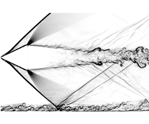
The detailed flow features have been reported in our previous work (Zuo et al. Reference Zuo, Memmolo, Huang and Pirozzoli2019). In this subsection, we limit ourselves to the description of the main characteristics, showing some slices for both mean and instantaneous configurations. Figure 4 shows the magnitude of the density gradient (numerical schlieren) on the symmetry plane, to highlight the overall wave system. Upstream of the interaction, the turbulent boundary layer develops and propagates downstream, creating numerous vortices lifting off the wall surface. At the impingement point, two reflected shock waves appear, indicating flow reversal. The first reflected shock is induced by the boundary layer separation, while the second shock is caused by the subsequent reattachment. Between these two shocks, an expansion fan is observed, as in the case of planar SBLI (Piponniau et al. Reference Piponniau, Dussauge, Debieve and Dupont2009; Pirozzoli & Bernardini Reference Pirozzoli and Bernardini2011a).

Figure 4.

Overall structure of the CSBLI. The cone geometry is blanked, and shock waves are shown by means of numerical schlieren, defined through the magnitude of the density gradient $(- 1.0 \times | {\boldsymbol {\nabla }\rho } |)$. Contours are in the range $-1.0 <- 1.0 \times | {\boldsymbol {\nabla } \rho } | < -0.04$, from black to white.

Focusing on the flow in the cone proximity, the expansion fan originating at its trailing edge is also seen clearly in figure 4, interacting with both the incident and reflected shocks. The cone wake is also seen interacting with the main stream, giving rise to a turbulent mixing layer. The flows shear each other in this mixing region, seeding streamwise vortices downstream. These vortices propagate up to the end of the computational domain. The reflected conical shock arising from the main interaction at approximately $x \approx 45 \delta _{in}$ impinges on the mixing layer and seems to disappear. Due to the expansion fan coming from the cone, the boundary layer relaxes under an FPG condition, becoming thinner, as shown clearly in figure 5, for the horizontal coordinate comprised between approximately $50\delta _{in}$ and $70 \delta _{in}$. After this location, the compression fan due to wake closure leads to a second APG region, and the boundary layer thickens again. The qualitative effects on the boundary layer thickness are revealed clearly in figure 5. The overall qualitative description of the flow is completed in supplementary movies 1 and 2, including the instantaneous streamwise velocity flow field and numerical schlieren defined through the magnitude of the density gradient (see supplementary movies available at https://doi.org/10.1017/jfm.2023.480).

Figure 5.

Mean Mach number contours in the streamwise, wall-normal plane, with $0.1< M<2.5$, and contour levels from blue to red. The black solid line indicates the sonic line.

3.2. Wall surface

The contours of the mean wall pressure are shown in figure 6(a). As the flow proceeds downstream, it encounters a first APG region (APG1), caused by the incident conical shock, which may be visualized by the black solid line in the same figure. This line is the nominal shock trace for inviscid flow, which for a conical shock intersecting a plane wall has the equation

(3.1)\begin{equation} (x-x_c)^2 - {\left( {\frac{z}{\tan \alpha}} \right)^2} = {\left( {\frac{h}{\tan \alpha}} \right)^2}, \end{equation}

where $x_c = 30 \, \delta _{in}$ is the cone leading edge, $\alpha = 41.85^\circ$ is the conical shock angle, and $h = 13.67 \, \delta _{in}$ is the distance of the cone axis from the wall. As can be seen, pressure after the shock trace is not uniform, but rather has a maximum on the symmetry line and decreases as the distance from the symmetry line increases, leading to a flow deflection away from the symmetry line. Moving along the streamwise direction, the flow then experiences an expansion, followed by a second horseshoe pattern of a high pressure region (APG2), corresponding to the compression waves generated by the wake closure behind the cone.

Figure 6.

(a) Contours of time-averaged wall pressure $p/p_{\infty }$, with $27$ contour levels, ranging from $0.6$ to $1.9$, from blue to red. The black line indicates the inviscid shock trace. (b) Contours of r.m.s. of wall pressure fluctuations, in dB scale, $p_{dB} = 20 \log _{10} (p' / (2 \times 10 ^{-5} \ \mathrm {Pa}))$, assuming $p_{\infty } = 1$ atm. Contour levels are shown from $150$ to $180$, from blue to red.

Contours of the r.m.s. of wall pressure fluctuations are shown in figure 6(b) in dB scale, assuming $p_{\infty } = 1$ atm. Strong spatial connection of this distribution is found with that of the vortical structures, shown in previous studies (Zuo et al. Reference Zuo, Memmolo, Huang and Pirozzoli2019). In particular, the largest values of $p_{rms}$ are found at the interacting shock foot, especially around the symmetry axis where the shock is stronger. Consistent decrease of the fluctuating pressure loads is observed past the incident shock in the FPG region, which is depleted with eddies, as shown in our previous paper (Zuo et al. Reference Zuo, Memmolo, Huang and Pirozzoli2019). The vortices tend to disappear in the FPG region, and to reform past the recompression shock; however, setting a lower threshold for the vortex identification criterion would still show weaker eddies in the expansion zone. A secondary peak is observed further downstream, corresponding to reformation of the vortical structures. Numerical artefacts should be noted at the side boundaries, which are due to the imperfect nature of the numerical radiating boundary conditions, especially in the presence of waves not propagating orthogonally to the computational boundary. These effects are, however, confined to a narrow layer adjacent to the boundaries.

3.3. Identification of flow regimes

The distribution of the r.m.s. of pressure fluctuations ($p_{rms}$) in the symmetry plane is reported, again in dB scale, in figure 7. The figure shows that the pressure fluctuations attain maximum values in the mixing layer near the primary interaction zone. The pressure fluctuations increases again at approximately $x/\delta _{in}=75$, in correspondence with the APG2 region. Large values of pressure fluctuations are also observed in the wake of the conical device that we use to generate the shock, as a result of vortex shedding. When analysing the boundary layer properties, with particular reference to the computation of the local maximum in the wall-normal direction of the Reynolds shear stress, the cone wake must not be considered, else it would lead to a miscalculation of the local maximum. A simple fix to this problem is to consider the maximum not over all $y$, but only up to the boundary layer edge.

Figure 7.

Contours of r.m.s. of pressure fluctuations ($p_{rms}$) in the symmetry plane, in dB scale, $p_{dB} = 20 \log _{10} (p_{rms} / (2 \times 10 ^{-5}\ \mathrm {Pa}))$, assuming $p_{\infty } = 1$ atm. Contour levels are shown from $150$ to $180$, from blue to red. The blank region corresponds to the shock generating device. Boxed numbers identify the streamwise stations 1–10, referenced in table 1.

For clarity in the illustration of the results, the boundary layer properties at selected streamwise stations are summarized in table 1. Station $1$ is the reference station where the profiles of figure 3 were taken, and together with station $2$, located just upstream of the start of APG1, they are representative of the first ZPG zone (ZPG1) of the flow. Stations 3 and 4 are taken in the virtual origins of separation and reattachment shocks, respectively, inside the APG1 zone. Stations 5 and 6 are inside the FPG zone of the flow, whereas stations 7 and 8 are inside the APG2 zone. Finally, stations 9 and 10 correspond to the second ZPG zone (ZPG2), in the supersonic recovery region.

The distributions of the average pressure coefficient $C_p = (p-p_\infty )/q_\infty$ and average friction coefficient $C_f = \tau _w /q_{\infty }$ ($q_\infty = 1/2 \rho _\infty u_\infty ^2$) on the symmetry line at the wall surface are reported in figure 8. At the wall surface, the wall shear stress $\tau _w$ is obtained as

(3.2)\begin{equation} \tau_w=\mu_w \left[ \left(\frac{\partial \bar u}{\partial y}\right)^2 + \left(\frac{\partial \bar w}{\partial y}\right)^2 \right]^{1/2}. \end{equation}

As found in experiments by Hale (Reference Hale2015) and Gai & Teh (Reference Gai and Teh2000), the wall pressure shown in figure 8(a) exhibits a distinctive N-wave signature, with a sharp peak right past the precursor shock generated at the cone apex, followed by an extended zone with FPG, and terminated by the trailing shock associated with recompression in the wake of the cone. From figure 8(b), it can be seen clearly that the boundary layer separates in the first APG zone. Based on the negative values of $C_f$, we can mark the separation region in the range $x/\delta _{in} = 43\unicode{x2013}45$, and $C_f$ attains its minimum value at $x/\delta _{in} \approx 44$. The skin friction then undergoes a sudden rise through the FPG region, after which it exhibits a drop, attaining a local minimum value in the second APG region, followed by a slow recovery process. This local minimum is, however, still higher than zero, reflecting that no mean separation occurs in the second APG zone. Upstream of the interaction zone and in the downstream ZPG2 region, the friction coefficient well follows the power-law behaviour predicted by simple theory (Smits & Dussauge Reference Smits and Dussauge2006), namely

(3.3)\begin{equation} C_f = k \, \textit{Re}_x^{{-}1/7}, \end{equation}

with $k = 0.0192$, with the obvious exception of the inflow region, where the boundary layer is not yet properly developed.

Figure 8.

Streamwise distributions of (a) pressure coefficient, (b) skin friction coefficient, and (c) Clauser pressure gradient parameter in the symmetry plane. The dash-dotted line in (b) represents (3.3).

Non-equilibrium states of boundary layers upon imposed pressure gradient are traditionally analysed in terms of Clauser pressure gradient parameter, defined as (Clauser Reference Clauser1954)

(3.4)\begin{equation} \beta = \frac{\delta^*}{\rho_w u_\tau^2}\,\frac{{\mathrm d} {\bar{p}}_w}{{\mathrm d} x} , \end{equation}

whose distribution along the symmetry axis is shown in figure 8(c). According to the DNS data, the flow field may be divided into five parts:

1. (i) ZPG1 for $x/\delta _{in}=0\unicode{x2013}39$, where $\beta \approx 0$;

2. (ii) APG1 for $x/\delta _{in}=39\unicode{x2013}46$, where $\beta$ exhibits a sharp positive peak;

3. (iii) FPG for $x/\delta _{in}=46\unicode{x2013}66$, where $\beta$ is negative as the flow accelerates;

4. (iv) APG2 for $x/\delta _{in}=66\unicode{x2013}80$, where $\beta$ attains a second positive peak;

5. (v) ZPG2 for $x/\delta _{in}>80$, where equilibrium conditions are recovered.

The mean velocity profiles across the interaction zone in the symmetry plane are reported in figure 9, for various streamwise stations. Before passing through the main interaction region, the velocity profiles do not show deviations with respect to canonical boundary layers. Moving downstream into the APG1 zone, the mean velocity profile shows negative values (station 4, $x/\delta _{in}=44.0$), highlighted in the inset plot, denoting the presence of a turbulent separation bubble. Passing through the FPG region, the boundary layer tends to become thinner under the effects of the expansion. The opposite behaviour is observed in the APG2 region, where the boundary layer thickness increases again.

Figure 9.

Mean velocity profiles at the wall in the symmetry plane at various streamwise stations. The horizontal coordinate is $\bar {u}/{u_e}$, with $| \bar {u}/{u_e} | <1$ inside the boundary layer. The vertical coordinate is $y/\delta _{ref}^*$, where $\delta _{ref}^*$ is the boundary layer thickness at station 1. For nomenclature, refer to table 1.

The structural modifications of turbulence statistics upon interaction with the conical shock wave are analysed here. In figure 10, we report the distributions of streamwise turbulence intensities at various streamwise stations on the symmetry plane. Upstream of the interaction zone, in the ZPG1 region, the profiles are again similar to each other, whereas in the mean separation region (station 4, at $x/\delta _{in}=44.0$), the streamwise turbulence intensity increases, and attains its maximum value $u''_{rms}/u_e=0.250$ at $y/\delta _{ref}^*=0.51$ in the boundary layer. In the FPG region, considerations similar to those made for figure 9 about the effects of the expansion on the boundary layer thickness can be made, especially by looking at the wall-normal distance of the maximum of the $u''_{rms}$ profile, with the maximum itself decreasing as well. In the APG2 region, the peak values increase again, assuming values below those obtained in the APG1 zone, with the peak value of the streamwise turbulence intensity $u''_{rms}/u_e=0.173$ at $y/\delta _{ref}^*=0.41$, for station 8.

Figure 10.

Streamwise turbulence intensities at various streamwise stations. The horizontal coordinate is $u''_{rms}/u_e$, in the range $0< u''_{rms}/u_e<0.25$. The vertical coordinate is $y/\delta _{ref}^*$, where $\delta _{ref}^*$ is the boundary layer thickness at station 1. For nomenclature, refer to table 1.

4.1. Pressure fluctuations distributions

The wall pressure fluctuations are shown in figure 11, under different normalizations. Regardless of the normalization, the field looks noisy, due to lack of directions with spatial homogeneity for the averaging. However, the overall behaviour is quite clear: with exception of some common behaviour, such as rise of the magnitude in the interaction regions, with the highest values shown in the first interaction because of the flapping motion of the separation bubble (Priebe & Martin Reference Priebe and Martin2012), one can notice distinctly that the pattern and the magnitude of $p_{rms}$ are heavily dependent on the chosen normalization. When the free-stream dynamic pressure is used for normalization, large variations are observed between the upstream ZPG region and the APG and FPG regions. When the wall shear stress is used, large changes are observed close to the separation and reattachment zones, where the shear stress is close to zero. When the local maximum Reynolds shear stress within the boundary layer is used for normalization, the pressure fluctuations retain $O(1)$ amplitude throughout, with exception of the separation and reattachment lines.

Figure 11.

Pressure fluctuations at the wall with different normalizations: (a) scaled by free-stream dynamic pressure, $0.004< p_{rms}/q_\infty <0.034$, exponential distribution; (b) scaled by wall-surface shear stress, $1.1< p_{rms}/|\tau _w|<80$, exponential distribution; (c) scaled by local maximum Reynolds shear stress $\tau _m = \max _y (-\bar \rho \,\widetilde {u''v''})$, $1.4 < p_{rms} / \tau _m < 4.2$, linear distribution.

For a more quantitative analysis, the data are now presented in the symmetry plane. Figure 12 shows r.m.s. pressure profiles in the wall-normal direction, up to $y/\delta _{in} = 4$, to exclude the wake region of the cone. In the ZPG regions (stations $1$ and $10$), the behaviour and the attained values are similar, but spread farther from the wall at station $10$ owing to higher Reynolds number. In the APG region corresponding to the first interaction with separated flow (station $4$), pressure fluctuations first increase slightly in a narrow region of the separated boundary layer to reach a plateau, then rise again up to a maximum, and finally decrease monotonically. The peak observed at station $4$ corresponds to intersection with the reflected shock. Similar amplification of pressure fluctuations in the presence of a separated turbulent boundary layer was also reported by Na & Moin (Reference Na and Moin1998) and Abe (Reference Abe2017). This behaviour is not observed at the other station representative of APG conditions (station $8$), where separation does not occur. Very low pressure fluctuations are obtained in the FPG region (station $6$), which is related to reduction of the number of vortical structures, as show in our previous work (Zuo et al. Reference Zuo, Memmolo, Huang and Pirozzoli2019).

Figure 12.

Profiles of r.m.s. pressure fluctuations at the streamwise stations $1$, $4$, $6$, $8$ and $10$, scaled by the free-stream dynamic pressure $q_\infty$. For nomenclature, refer to table 1.

The amplitude of the wall pressure fluctuations in the symmetry plane, as shown by the solid line in figure 13, is nearly constant in the incoming ZPG region, where $p_{rms}=0.0072 q_\infty$, corresponding to an overall sound pressure level ($p_{dB} = 20 \log _{10} (p / (2 \times 10 ^{-5}\ \mathrm {Pa}))$) of approximately $160.6$ dB. In the same figure we also show the wall shear stress premultiplied by the factors $2.15$ and $2.5$. We find that for the incoming boundary layer, there is overlap between $p_{rms}$ and $2.15 \tau _w$, in agreement with the low-speed boundary layer DNS of Pirozzoli & Bernardini (Reference Pirozzoli and Bernardini2011b), who reported ${p_{rms} = 2.2\tau _w}$ for $\textit {Re}_\tau \leq 250$, whereas in the second ZPG zone, we find $p_{rms} \approx 2.5 \tau _w$, which again is in good agreement with what was obtained by Bernardini et al. (Reference Bernardini, Pirozzoli and Grasso2011) ($p_{rms} = 2.5\tau _w$) and by Farabee & Casarella (Reference Farabee and Casarella1991) ($p_{rms} = 2.55\tau _w$) for $\textit {Re}_\tau \leq 333$. As a note of caution, we point out that the value of $p_{rms}/\tau _w$ depends not only on Reynolds number, but also on the Mach number. Bernardini & Pirozzoli (Reference Bernardini and Pirozzoli2011) analysed supersonic adiabatic turbulent boundary layers at Mach numbers $M_\infty = 2,3,4$ by DNS, spanning a relatively large range of Reynolds numbers, namely $\textit {Re}_\tau = 250\unicode{x2013}1100$. They found that at the wall, the value of $p_{rms}/\tau _w$ is affected mainly by Reynolds number variation, but increasing the Mach number also yields a slight increase. The range of values reported in that study is $p_{rms}/\tau _w = 2.2\unicode{x2013}2.8$, which is in good agreement with the present data. In the APG1 zone, the wall pressure fluctuations attain a maximum value $p_{rms}=0.031 q_\infty$, corresponding to an overall sound pressure level of approximately $173.3$ dB. The minimum value is attained in the FPG zone where $p_{rms} \approx 0.0044 q_\infty$, corresponding to an overall sound pressure level of approximately $156.3$ dB. In the APG2 zone, a second local maximum $p_{rms} \approx 0.0115 q_\infty$ is attained, corresponding to an overall sound pressure level of approximately $164.7$ dB. The present DNS results in the separation region ($x/\delta _{in} = 43\unicode{x2013}45$) show a $p_{rms}$ varying between $0.018$ and $0.032$, in good agreement with the Simpson et al. (Reference Simpson, Ghodbane and McGrath1987) experimental data, in which the range is $0.020\unicode{x2013}0.031$.

Figure 13.

Profile of $p_{rms}/p_{\infty }$ (solid line), $2.15 \tau _w$ (dashed line) and $2.5 \tau _w$ (dash-dotted line), normalized by $\tau _m = \max _y (-\bar {\rho }\,\widetilde {u''v''})$ (dash-dot-dotted line). The vertical dashed lines denotes particular values of $\textit {Re}_\tau$.

For completeness, figure 13 also shows the r.m.s. of wall pressure fluctuations in the symmetry plane, normalized by the local maximum Reynolds shear stress $-\bar {\rho }\,\widetilde {u''v''}_{max}$. In this case, a different scale is employed because of the different amplitudes involved. As observed by Simpson et al. (Reference Simpson, Ghodbane and McGrath1987), the maximum Reynolds shear stress appears to be a better scale to normalize wall pressure fluctuations in separated turbulent boundary layers. With this scaling, the r.m.s. of wall pressure fluctuations in the experiments of Simpson et al. (Reference Simpson, Ghodbane and McGrath1987) varied from $4.0$ to $5.5$ in the separation region. The present DNS results have normalized values between $2.5$ and $4.0$, i.e. somewhat less. However, Na & Moin (Reference Na and Moin1998) also reported that the wall pressure fluctuations normalized by the local maximum Reynolds shear stress vary from $2.5$ to $3.0$ based on their DNS data ($\textit {Re}_\theta = 670$, the same Reynolds number as our DNS at reference station), which is in good agreement with our results. As Na & Moin (Reference Na and Moin1998) discussed, this sizeable difference may be explained as due to low-Reynolds-number effects. In fact, Choi & Moin (Reference Choi and Moin1990) compared available experimental and numerical data, and reported that variation of $p_{rms}$ with the Reynolds numbers is rather large ($p_{rms}$ at $\textit {Re}_\theta = 13\,200$ is approximately $2.5$ times that at $\textit {Re}_\theta = 290$). Logarithmic growth of the pressure variance with $\textit {Re}_\tau$ in canonical pipe flow has been reported recently by Yu, Ceci & Pirozzoli (Reference Yu, Ceci and Pirozzoli2022). Considering the large difference in Reynolds numbers, the present results are compatible with the variation reported by Choi & Moin (Reference Choi and Moin1990).

4.2. Frequency spectra

Time series of wall pressure fluctuations in the symmetry plane at several different streamwise locations are reported in figure 14, which shows a wide range of time scales. Note that, as shown in figure 8(b), the boundary layer is separated at $x/{\delta _{in}} = 44$. To help the visualization, the vertical range is not the same in the various plots. As one moves towards the separation region, the frequency of the oscillations decreases noticeably, and the amplitude in the interaction zone increases significantly. Inside the separation region, the signal is dominated by low-frequency motions, as in the case of low-Reynolds-number turbulent boundary layer separation (Na & Moin Reference Na and Moin1998). The long-time-scale behaviour noticed in figure 14(b) is associated with the movement of large-scale structures generated in the shear layer due to an inflectional hydrodynamic instability as in mixing layers. The signal in the second APG region (figure 14d) is again dominated by low-frequency motions; similar behaviour is observed in spanwise homogeneous compression ramp SBLI (Priebe & Martin Reference Priebe and Martin2012; Priebe et al. Reference Priebe, Tu, Rowley and Martin2016) and other axisymmetric interactions (Estruch-Samper & Chandola Reference Estruch-Samper and Chandola2018; Huang & Estruch-Samper Reference Huang and Estruch-Samper2018). The presence of low-frequency motions implies that a large statistical sample is required to get converged statistics inside the separation bubble. The amplitude of pressure fluctuation decreases in the FPG region (figure 14c), and the signal there is dominated by high-frequency motions again.

Figure 14.

Time histories of wall pressure fluctuations in the symmetry plane. To facilitate visualization, the vertical ranges take different values: (a) $x/\delta _{in} = 27.5$, ZPG1 region; (b) $x/\delta _{in} = 44$, APG1 region; (c) $x/\delta _{in} = 62$, FPG region; (d) $x/\delta _{in} = 75$, APG2 region.

The PSD of the wall pressure signal (say, $E(f; x, y)$, where $f$ is the frequency) has been estimated for locations ranging from the upstream flow to the downstream relaxation region, according to the Welch method, as suggested by Choi & Moin (Reference Choi and Moin1990) and Bernardini et al. (Reference Bernardini, Pirozzoli and Grasso2011), hence subdividing the overall pressure record (covering a time span $140\delta _0^*/{u_\infty }$) into twelve overlapping segments. As shown by Bernardini et al. (Reference Bernardini, Pirozzoli, Quadrio and Orlandi2013), the frequency spectra of the wall pressure in wall-bounded flows obtained with finite-difference solvers may be contaminated from numerical dispersion errors. Hence frequencies higher than $0.1 u_e / \delta ^*$ are hereafter removed. The wall pressure spectrum for all numerical probes is shown in figure 15 as a function of both Strouhal numbers, $St_{\delta }=f \delta _{ref}/{u_\infty }$ and $St_L=f L/{u_\infty }$, with $L$ the distance between the separation point and the nominal shock impingement location, and of the scaled streamwise coordinate $x/ \delta _{in}$. It should be noted that a premultiplied representation is used ($\,f\,E(f)$), such that equal areas yield equal contribution to the pressure variance when frequency is reported on a logarithmic scale. Several regions can be identified, which are characterized by different characteristic time scales.

1. (i) A region dominated by high-frequency motions, $x/\delta _{in}<40$, corresponding to the incoming turbulent boundary layer, with a peak at $St \approx 1$ associated with the energetic turbulent structures of the boundary layer (Gaitonde & Adler Reference Gaitonde and Adler2023). It should be emphasized that no significant energy was found in the range $0.01< St_L<0.1$ in the upstream boundary layer.

2. (ii) The zone around the foot of the reflected shock, $40< x/\delta _{in}< 50$, which is characterized by strong low-frequency motions, especially near the separation point, and associated with flapping motion of the reflected shock system, similar to what is found in more canonical planar SBLIs (Dupont et al. Reference Dupont, Haddad and Debieve2006; Clemens & Narayanaswamy Reference Clemens and Narayanaswamy2014). The PSD appears to be more broadbanded, and its peak is clearly shifted to lower frequencies due to the thickening of the boundary layer. A limited part of the broadband energy in the premultiplied spectra is found close to the foot of the reflected shock at frequencies that are two orders of magnitude lower than the turbulent structures of the incoming boundary layer.

3. (iii) The FPG zone, $50< x/\delta _{in}< 65$, in which low and intermediate scales are dominant, whose frequencies range between the low ones typical of the shock motion and the high ones associated with the incoming turbulence.

4. (iv) The secondary interaction zone, $65< x/\delta _{in}< 80$, which shows the same behaviour as zone (ii), hence characterized by frequencies that are 1–2 orders of magnitude less than the turbulent structures of the incoming boundary layer.

5. (v) A relaxation zone, $x/\delta _{in}> 80$, where the high-frequency motions developing inside the interaction zones become dominant again as the boundary layer returns to an equilibrium state.

Figure 15.

Contours of premultiplied PSD ($\,f\,E(f)$) of wall pressure fluctuations along the symmetry plane. The red line denotes the mean separation location, and the green line the mean reattachment location. The blue cross marks the position of the low-frequency peak near the separation line; $St_L=f L/{u_\infty }$ is the Strouhal number based on the interaction length scale.

In this respect, we note that in spanwise homogeneous SBLIs, typical low-frequency oscillations arising around the separation point have a typical frequency $St_L \approx 0.03$, hence two orders of magnitude less than the dominant frequencies in the boundary layer. Experiments and numerical studies of SBLIs in the presence of flow skewing, including compression ramps (Erengil & Dolling Reference Erengil and Dolling1993; Vanstone et al. Reference Vanstone, Saleem, Seckin and Clemens2017; Adler & Gaitonde Reference Adler and Gaitonde2018, Reference Adler and Gaitonde2020), sharp fins (Schmisseur & Dolling Reference Schmisseur and Dolling1994; Gaitonde et al. Reference Gaitonde, Shang, Garrison, Zheltovodov and Maksimov1999; Arora, Mears & Alvi Reference Arora, Mears and Alvi2019) and swept impinging oblique SBLIs (Doehrmann et al. Reference Doehrmann, Padmanabhan, Threadgill and Little2018; Padmanabhan et al. Reference Padmanabhan, Maldonado, Threadgill and Little2021), rather seem to indicate suppression of the low-frequency peak in the presence of 3-D effects, on account of a topological change of the separation bubble from a closed to an open type. Recently, Ceci et al. (Reference Ceci, Palumbo, Larsson and Pirozzoli2023) have proposed that the typical frequencies increase with the skew angle, on account of propagation spanwise travelling disturbances. Figure 15 shows evidence for 2-D-like dynamics in the proximity of the separation and reattachment points, as well as in the secondary APG region. This is the likely consequence that the dynamics in the symmetry plane is similar to nominally 2-D interactions.

To analyse the pressure spectra in greater detail, a comparison in the ZPG region with well-established results is reported in figure 16. The shapes of the frequency spectra at stations $1$ and $10$, corresponding to ZPG conditions, adopting two different normalizations, conform in general terms to those observed in low-speed boundary layers. In figure 16(a), pressure is scaled with respect to $\tau _w^2$ and the reference time is $\delta _v / u_\tau$. In figure 16(b), the mixed time scale $\delta /u_\tau$ is used instead. Good collapse with the experimental data of Gravante et al. (Reference Gravante, Naguib, Wark and Nagib1998) and previous DNS database of Bernardini et al. (Reference Bernardini, Pirozzoli and Grasso2011) at comparable friction Reynolds number with respect to station $10$, is observed in the middle- and high-frequency end of the spectrum, which is dominated by the influence of near-wall motions (Blake Reference Blake2017), when pressure is scaled with respect to the wall friction, and viscous time units are used for normalizations. The use of a ‘mixed’ time scale $(\delta / u_\tau )$, which is expected to yield better collapse of the low-/intermediate-frequency end of the spectrum, still yields a satisfactory comparison with the experimental data of Gravante et al. (Reference Gravante, Naguib, Wark and Nagib1998). As predicted theoretically by Blake (Reference Blake2017), the spectrum approximately drops off as $\omega ^{-5}$ at high frequencies. In this range of scales, inner scaling leads to good collapse between different Reynolds numbers, which is lost with use of the mixed time scale. The low-frequency $\omega ^2$ scaling, reported in an experiment for incompressible turbulent boundary layer by Farabee & Casarella (Reference Farabee and Casarella1991), is not observed here, possibly because of limited duration of the time sample. Overall, the agreement between the spectrum at station $10$ with reference data is excellent, which corroborates the quality of present results.

Figure 16.

Wall pressure frequency spectrum in ZPG regions. Station 1 is at Reynolds number $\textit {Re}_\tau = 160$. Station 10 is at Reynolds number $\textit {Re}_\tau = 280$, at flow conditions comparable with Bernardini et al. (Reference Bernardini, Pirozzoli and Grasso2011) at $\textit {Re}_\tau = 340$ (green solid circles) and Gravante et al. (Reference Gravante, Naguib, Wark and Nagib1998) at $\textit {Re}_\tau = 715$ (blue open triangles). Pressure is scaled with respect to $\tau _w^2$, and the reference time is $\delta _v / u_\tau$ in (a) and $\delta / u_\tau$ in (b).

The wall frequency spectra in the APG1 regions are reported in figure 17, under condition of boundary layer separation. To verify the possible occurrence of universal scaling laws, the spectra are now normalized with respect to either the local external dynamic pressure $q_e$, or the local maximum shear stress $\tau _m$. In both cases, the local (outer) reference time $\delta ^* / u_e$ is adopted. The latter scaling is expected to partially account for non-equilibrium effects caused by the APG (Mabey Reference Mabey1982), as indeed is verified by Simpson et al. (Reference Simpson, Ghodbane and McGrath1987) and Na & Moin (Reference Na and Moin1998). The shape of pressure spectra in the APG1 region is similar to that observed in the ZPG regions. Reasonable universality is achieved when pressure is scaled with respect to $\tau _m$, especially at low and middle frequencies, whereas at high frequencies, significant scatter is observed, maybe caused by turbulent boundary layer separation ($x/\delta _{in}=44\unicode{x2013}45$). On the other hand, when pressure is normalized by $q_{\infty }$, an increase of the PSD progressing in the streamwise direction is observed at all frequencies, as also reported by Na & Moin (Reference Na and Moin1998) and Bernardini et al. (Reference Bernardini, Pirozzoli and Grasso2011). This indicates that the free-stream dynamic pressure has less direct influence on the wall pressure spectra than the local maximum shear stress inside the separation bubble.

Figure 17.

Frequency spectra of the wall pressure at various stations in the APG1 region. Local outer scaling is used, and pressure is scaled by (a) $q_e^2$ or (b) $\tau _m^2$. Data are taken at $x/\delta _{in}=41, 42, 43, 44, 45, 46$.

The spectra downstream of the reattachment point in the FPG region are reported in figure 18. Similar to the observation made for the APG1 region, reasonable universality is obtained when pressure is scaled with respect to $\tau _m$ at low and middle frequencies. It should be noted that when pressure is normalized by $q_e$, a decrement of the PSD progressing in the streamwise direction is observed at all frequencies. This is the opposite behaviour with respect to the APG1 regions, indicating that the pressure gradient has a strong effect on the power spectra of wall pressure fluctuations.

Figure 18.

Frequency spectra of the wall pressure at various stations in the FPG region. Local outer scaling is used, and pressure is scaled by (a) $q_e^2$ or (b) $\tau _m^2$. Data are taken at $x/\delta _{in}=48, 50, 52, 54, 56, 58$.

The frequency spectra in the APG2 region without turbulent separation are shown in figure 19. The data nearly collapse to a single distribution regardless of the normalization at all frequencies, indicating that the wall pressure field has recovered past the separation. Actually, self-similar structure of the boundary layer was also found in our previous study (Zuo et al. Reference Zuo, Memmolo, Huang and Pirozzoli2019).

Figure 19.

Frequency spectra of the wall pressure at various stations in the APG2 region. Local outer scaling is used, and pressure is scaled by (a) $q_e^2$ or (b) $\tau _m^2$. Data are taken at $x/\delta _{in}=71, 72, 73, 74, 75, 76$.

4.3. Two-point correlations

The spatial imprinting of pressure fluctuations at the wall is investigated in this subsection through the analysis of the two-point space–time correlation coefficient, defined as

(4.1)\begin{equation} R_{p p}\left(x ; r_1, r_2, r_3, \tau\right)=\frac{\left\langle p^{\prime}(x, 0, z, t)\, p^{\prime}(x+r_1, r_2, z+r_3, t+\tau)\right\rangle}{p_{r m s}(x, 0)\,p_{r m s}(x+r_1, r_2)}, \end{equation}

where $(r_1, r_2, r_3)$ is the spatial separation vector, and $\tau$ is the time delay.

Iso-lines of the two-point spatial correlation in the wall plane $R_{p p}(x ; r_{1}, 0, r_{3}, 0)$ are displayed at various stations in figure 20. Differences among the various flows are visible, the dominant effect being due to the pressure gradient. In the ZPG region (station $1$), the contours of $R_{pp}$ are roughly circular at small separations, indicating near-isotropy of the pressure-carrying eddies (Probsting et al. Reference Probsting, Scarano, Bernardini and Pirozzoli2013). At larger separations in the APG1 region, the iso-lines become more elongated in the spanwise direction, reflecting an anisotropic state of the large structures. In the APG1 region (mean flow separation), an increase of the characteristic pressure length scales is observed, and the iso-lines become more elongated in the spanwise direction. Downstream of the bubble (station $3$), where the flow field redevelops under strong FPG, the flow begins to recover. The shapes of iso-lines slowly revert back to those of attached boundary layers. However, the iso-lines is still elongated to a certain extent in the spanwise direction. In the APG2 region (instantaneous flow reversal), an elongated two-point correlation in the spanwise direction is again observed. In the ZPG2 region, the boundary layer returns to an equilibrium state Zuo et al. (Reference Zuo, Memmolo, Huang and Pirozzoli2019), and the spatial coherence of the pressure field begins to decrease consistently. However, spatial coherences of ZPG1 and ZPG2 differ slightly, due mainly to the effect of the different $Re_{\tau }$. As proven by Bernardini & Pirozzoli (Reference Bernardini and Pirozzoli2011), as $Re_{\tau }$ increases, the spatial coherence of the pressure field is found to decrease.

Figure 20.

Iso-lines of two-point pressure correlation $R_{p p}(x ; r_{1}, 0, r_{3}, 0)$ at streamwise stations $1$, $3$, $5$, $7$ and $9$ in (a–d), respectively, are shown. Ten equally spaced contour levels are shown, from $-0.1$ to $0.9$ (the zero iso-line is omitted).

4.4. Space–time correlations

Contour lines of the space–time correlation coefficient $R_{p p}(x ; r_{1}, 0, 0, \tau )$ are shown in figure 21, including lines with slope equal to the convection velocity $U_c$. Proceeding as in Bernardini & Pirozzoli (Reference Bernardini and Pirozzoli2011), we define the convection velocity corresponding to a given time delay $\tau$ as the ratio $r_1/\tau$ taken at the value of $r_1$ where a local maximum is attained. The convection velocities obtained at different stations are reported in table 2. As for the two-point spatial correlations, the shape of the maps reflects the convective nature of the pressure field, which is characterized by coherent downstream propagation of pressure-carrying eddies. The space–time organization of the pressure field upstream of the interaction is similar to that observed in the ZPG compressible boundary layer (Bernardini & Pirozzoli Reference Bernardini and Pirozzoli2011; Duan, Choudhari & Zhang Reference Duan, Choudhari and Zhang2016).

Figure 21.

(a–e) Iso-lines of the space–time correlation $R_{p p}(x ; r_{1}, 0, 0, \tau )$ at streamwise stations $1$, $3$, $5$, $7$ and $9$, respectively. Ten equally spaced contour levels are shown, from $-0.1$ to $0.9$ (the zero iso-line is omitted). The slope of the red line represents the magnitude of convection velocity.

Table 2.

Local convection velocity of wall pressure fluctuations at different locations, normalized by local free-stream velocity $U_\infty$.

The convection velocities of wall pressure fluctuations decrease as the pressure gradient increases. When in the FPG region, the convection velocity shows an increasing trend, consistently with the results of Na & Moin (Reference Na and Moin1998) and Bernardini & Pirozzoli (Reference Bernardini and Pirozzoli2011), whereas coherence tends to decrease while progressing downstream, as seen by the increased spreading of the contour lines, which is most apparent in the separated (APG1) region.

From the maps of figure 21, one can deduce the characteristic convection velocities ($U_c$) of the eddies. The convection speed of the large-scale disturbances is associated with low frequencies (Na & Moin Reference Na and Moin1998; Bernardini et al. Reference Bernardini, Pirozzoli and Grasso2011). When data are scaled with respect to the free-stream velocity ($U_\infty$), pressure disturbances are found to propagate at speeds in the range $0.6U_\infty \unicode{x2013}0.7 U_\infty$. Such behaviour is consistent with the results of Schloemer (Reference Schloemer1967), Na & Moin (Reference Na and Moin1998) and Bernardini et al. (Reference Bernardini, Pirozzoli and Grasso2011), who found that, compared with the canonical boundary layer case, the convection velocities are higher under FPG and lower under APG.