


Crossref Citations
This article has been cited by the following publications. This list is generated based on data provided by Crossref.
Henry, Pierre-Yves
Aberle, Jochen
Navaratnam, Christy Ushanth
Ruther, Nils
Paquier, A.
and
Rivière, N.
2018.
Hydraulic physical model production with Computer Numerically Controlled (CNC) manufacturing techniques.
E3S Web of Conferences,
Vol. 40,
Issue. ,
p.
05065.
Verschoof, Ruben A.
Zhu, Xiaojue
Bakhuis, Dennis
Huisman, Sander G.
Verzicco, Roberto
Sun, Chao
and
Lohse, Detlef
2018.
Rough-wall turbulent Taylor-Couette flow: The effect of the rib height.
The European Physical Journal E,
Vol. 41,
Issue. 10,
Praks, Pavel
and
Brkić, Dejan
2018.
One-Log Call Iterative Solution of the Colebrook Equation for Flow Friction Based on Padé Polynomials.
Energies,
Vol. 11,
Issue. 7,
p.
1825.
Brkić, Dejan
and
Praks, Pavel
2018.
Unified Friction Formulation from Laminar to Fully Rough Turbulent Flow.
Applied Sciences,
Vol. 8,
Issue. 11,
p.
2036.
Hamed, Ali M.
Peterlein, Adam M.
and
Randle, Lindsey V.
2019.
Turbulent boundary layer perturbation by two wall-mounted cylindrical roughness elements arranged in tandem: Effects of spacing and height ratio.
Physics of Fluids,
Vol. 31,
Issue. 6,
Peeters, J.W.R.
and
Sandham, N.D.
2019.
Turbulent heat transfer in channels with irregular roughness.
International Journal of Heat and Mass Transfer,
Vol. 138,
Issue. ,
p.
454.
Toussaint, D.
Chedevergne, F.
and
Léon, O.
2020.
Analysis of the different sources of stress acting in fully rough turbulent flows over geometrical roughness elements.
Physics of Fluids,
Vol. 32,
Issue. 7,
Alves Portela, F.
and
Sandham, N.D.
2020.
A DNS/URANS approach for simulating rough-wall turbulent flows.
International Journal of Heat and Fluid Flow,
Vol. 85,
Issue. ,
p.
108627.
Adams, David Lawson
2020.
Toward bed state morphodynamics in gravel-bed rivers.
Progress in Physical Geography: Earth and Environment,
Vol. 44,
Issue. 5,
p.
700.
Skeide, Arne Kilvik
Bardal, Lars Morten
Oggiano, Luca
and
Hearst, R. Jason
2020.
The significant impact of ribs and small-scale roughness on cylinder drag crisis.
Journal of Wind Engineering and Industrial Aerodynamics,
Vol. 202,
Issue. ,
p.
104192.
Aberle, Jochen
Henry, Pierre-Yves
Kleischmann, Fabian
Navaratnam, Christy Ushanth
Vold, Mari
Eikenberg, Ralph
and
Olsen, Nils Reidar Bøe
2020.
Experimental and Numerical Determination of the Head Loss of a Pressure Driven Flow through an Unlined Rock-Blasted Tunnel.
Water,
Vol. 12,
Issue. 12,
p.
3492.
Jayaraman, Balaji
and
Khan, Saadbin
2020.
Direct numerical simulation of turbulence over two-dimensional waves.
AIP Advances,
Vol. 10,
Issue. 2,
Kadivar, Mohammadreza
Tormey, David
and
McGranaghan, Gerard
2021.
A review on turbulent flow over rough surfaces: Fundamentals and theories.
International Journal of Thermofluids,
Vol. 10,
Issue. ,
p.
100077.
Aghaei Jouybari, Mostafa
Yuan, Junlin
Brereton, Giles J.
and
Murillo, Michael S.
2021.
Data-driven prediction of the equivalent sand-grain height in rough-wall turbulent flows.
Journal of Fluid Mechanics,
Vol. 912,
Issue. ,
Wang, Xiaojia
and
Christov, Ivan C.
2021.
Reduced models of unidirectional flows in compliant rectangular ducts at finite Reynolds number.
Physics of Fluids,
Vol. 33,
Issue. 10,
Alves Portela, F.
Busse, A.
and
Sandham, N. D.
2021.
Numerical study of Fourier-filtered rough surfaces.
Physical Review Fluids,
Vol. 6,
Issue. 8,
Jelly, T.O.
Ramani, A.
Nugroho, B.
Hutchins, N.
and
Busse, A.
2022.
Impact of spanwise effective slope upon rough-wall turbulent channel flow.
Journal of Fluid Mechanics,
Vol. 951,
Issue. ,
Aberle, Jochen
Branß, Till
Eikenberg, Ralph
Henry, Pierre-Yves
and
Olsen, Nils Reidar B.
2022.
Directional dependency of flow resistance in an unlined rock blasted hydropower tunnel.
Journal of Hydraulic Research,
Vol. 60,
Issue. 3,
p.
504.
Yang, Jiasheng
Stroh, Alexander
Chung, Daniel
and
Forooghi, Pourya
2022.
Direct numerical simulation-based characterization of pseudo-random roughness in minimal channels.
Journal of Fluid Mechanics,
Vol. 941,
Issue. ,
Aghaei-Jouybari, Mostafa
Seo, Jung-Hee
Yuan, Junlin
Mittal, Rajat
and
Meneveau, Charles
2022.
Contributions to pressure drag in rough-wall turbulent flows: Insights from force partitioning.
Physical Review Fluids,
Vol. 7,
Issue. 8,
1 Introduction
Engineers do not currently have the ability to accurately predict the drag of a generic rough surface. After decades of detailed measurements and recent computations of boundary layer flow over rough surfaces, the friction drag on a surface is only accurately known for the tested surfaces.
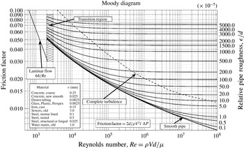
Figure 1. Reprinted with permission from L. F. Moody, Friction factors for pipe flow, Trans. ASME, vol. 66, 1944, pp. 671–684. Copyright 1944 ASME.
Engineering predictions of surface roughness is generally characterized by $k_{s}$
, the equivalent sand grain roughness height. This is the size of uniformly packed sand grains tested by Nikuradse (Reference Nikuradse1933) that produces the same frictional drag in the fully rough regime. Therefore,
$k_{s}$
, the equivalent sand grain roughness height. This is the size of uniformly packed sand grains tested by Nikuradse (Reference Nikuradse1933) that produces the same frictional drag in the fully rough regime. Therefore, $k_{s}$
is a hydraulic scale, not a physical scale, and this is what is listed on the Moody diagram (Reference Moody1944) (figure 1) as
$k_{s}$
is a hydraulic scale, not a physical scale, and this is what is listed on the Moody diagram (Reference Moody1944) (figure 1) as $\unicode[STIX]{x1D716}$
, the equivalent roughness height. I suspect that the word equivalent has often been ignored and the words roughness height have been used. If this is the case, then which roughness height? The mean, the peak-to-trough, or the root mean square (r.m.s.) roughness height? Even if you select one of these roughness scales, all are dependent to some extent on the spatial sample size of your measurement region. Therefore, the Moody diagram is only accurate for surfaces with known
$\unicode[STIX]{x1D716}$
, the equivalent roughness height. I suspect that the word equivalent has often been ignored and the words roughness height have been used. If this is the case, then which roughness height? The mean, the peak-to-trough, or the root mean square (r.m.s.) roughness height? Even if you select one of these roughness scales, all are dependent to some extent on the spatial sample size of your measurement region. Therefore, the Moody diagram is only accurate for surfaces with known $k_{s}$
in the fully rough regime.
$k_{s}$
in the fully rough regime.
The transitionally rough regime poses its own set of challenges. The transitionally rough regime is characterized by contributions from viscous and form drag on the roughness elements. At low Reynolds numbers, viscosity damps out flow disturbances caused by surface roughness. For these conditions, the flow is classified as hydraulically smooth. As Reynolds number increases, the turbulent eddies caused by the roughness elements are not fully damped by viscosity and form drag on the roughness contributes to the overall drag, increasingly with increased Reynolds number. Eventually, form drag is the dominant mechanism, and the flow becomes fully rough. The mechanisms responsible for this transition from hydraulically smooth to fully rough are not fully understood. Do roughness effects occur gradually as the roughness Reynolds number ( $k^{+}=U_{\unicode[STIX]{x1D70F}}k/\unicode[STIX]{x1D708}$
, where
$k^{+}=U_{\unicode[STIX]{x1D70F}}k/\unicode[STIX]{x1D708}$
, where $k$
is the roughness height,
$k$
is the roughness height, $U_{\unicode[STIX]{x1D70F}}$
is the friction velocity and
$U_{\unicode[STIX]{x1D70F}}$
is the friction velocity and $\unicode[STIX]{x1D708}$
is the kinematic viscosity) increases, as assumed by the Colebrook (Reference Colebrook1939) roughness function (used in the Moody diagram), or is the onset of roughness effects more abrupt, occurring at a finite
$\unicode[STIX]{x1D708}$
is the kinematic viscosity) increases, as assumed by the Colebrook (Reference Colebrook1939) roughness function (used in the Moody diagram), or is the onset of roughness effects more abrupt, occurring at a finite $k^{+}$
as represented by a Nikuradse (Reference Nikuradse1933) roughness function?
$k^{+}$
as represented by a Nikuradse (Reference Nikuradse1933) roughness function?
It has been shown that the onset of roughness effects, the shape of the roughness function in the transitionally rough regime and the Reynolds number where the flow becomes fully rough are highly dependent on roughness geometry (Flack & Schultz Reference Flack and Schultz2014). Since there are a myriad of roughness geometries, a way is needed to categorize surface roughness by easy to measure statistical or roughness feature properties. Additionally the measurement region upon which these properties are based should be identified, and potentially scales that do not contribute to the drag need to be removed before determining surface statistics. This filter should also be based on a roughness scale. There are a number of issues that need to be addressed before developing a robust engineering correlation, hence the reason that the contributions by Thakkar, Busse & Sandham (Reference Thakkar, Busse and Sandham2018) (for example, dispersive sheer stress as shown in the figure by the title) and other recent simulations of rough wall flows are so important. Realistic rough surfaces at relevant Reynolds numbers are being computed and there is hope in making headway towards identifying roughness scales to inform engineering predictions of surface drag.
2 Overview
A number of recent simulations over complex roughness have been performed with the goal of understanding the near wall turbulence and developing predictive correlations for drag. Mathematically generated surfaces with a range of scales allow for parametrically changing surface parameters. Anderson & Meneveau (Reference Anderson and Meneveau2011) performed a large eddy simulation (LES) for flow over a multi-scale, fractal-like roughness, similar to the range of scales in natural terrains. Realistic roughness was studied by Yuan & Piomelli (Reference Yuan and Piomelli2011) using LES for roughness replicated from hydraulic turbine blades, with surface features parametrically changed to study the influence of roughness slope on the surface drag. Three-dimensional sinusoidal roughness in the transitionally rough regime was investigated using direct numerical solution (DNS) by Chan et al. (Reference Chan, MacDonald, Chung, Hutchins and Ooi2015) and MacDonald et al. (Reference MacDonald, Chung, Chan, Hutchins and Ooi2016). It was shown in these studies that the roughness function could be accurately determined using the minimal-span channel technique (Chung et al. Reference Chung, Chan, MacDonald, Hutchins and Ooi2015) which allows for low Reynolds number simulations ( $Re_{\unicode[STIX]{x1D70F}}=U_{\unicode[STIX]{x1D70F}}h/\unicode[STIX]{x1D708}=180$
, where
$Re_{\unicode[STIX]{x1D70F}}=U_{\unicode[STIX]{x1D70F}}h/\unicode[STIX]{x1D708}=180$
, where $h$
is the channel half height). This is encouraging since a large number of parameters can be investigated at a lower computational cost. Forooghi et al. (Reference Forooghi, Stroh, Magagnato, Jakirlic and Frohnapfel2017) also used DNS at low
$h$
is the channel half height). This is encouraging since a large number of parameters can be investigated at a lower computational cost. Forooghi et al. (Reference Forooghi, Stroh, Magagnato, Jakirlic and Frohnapfel2017) also used DNS at low $Re_{\unicode[STIX]{x1D70F}}$
to determine the equivalent sand grain roughness for randomly distributed roughness elements of random size and prescribed shape. Correlations are presented considering roughness heights, slopes, density and moments of the surface elevation p.d.f.
$Re_{\unicode[STIX]{x1D70F}}$
to determine the equivalent sand grain roughness for randomly distributed roughness elements of random size and prescribed shape. Correlations are presented considering roughness heights, slopes, density and moments of the surface elevation p.d.f.
Thakkar et al. (Reference Thakkar, Busse and Sandham2018) are the first to use DNS to study a realistic irregular roughness, similar to the sand grain roughness of Nikuradse (Reference Nikuradse1933), for the entire range of roughness Reynolds numbers from hydraulically smooth to fully rough. This is an extension of their previous work (Thakkar, Busse & Sandham Reference Thakkar, Busse and Sandham2017) where they presented roughness results in the upper part of the transitionally rough regime and the fully rough regime for grit blasted and graphite surfaces. DNS with engineering roughness is a true advancement, and they have developed techniques to tile these surfaces within the computational domain. The grit blasted surface is deemed Nikuradse-like because it follows the Nikuradse roughness function with $k_{s}^{+}=0.87k^{+}$
. The authors expect other sand-grain-like surfaces to have similar behaviour. The interesting question is what makes a surface sand-grain-like: sharp protrusions, close packing, a distinct range of scales, positive or negative skewness?
$k_{s}^{+}=0.87k^{+}$
. The authors expect other sand-grain-like surfaces to have similar behaviour. The interesting question is what makes a surface sand-grain-like: sharp protrusions, close packing, a distinct range of scales, positive or negative skewness?
3 Future
Tremendous progress has been made in the prediction of frictional drag on rough surfaces. The way forward is to study both realistic roughness and mathematically generated surfaces that contain a range of surface features. Recent computations have shown that drag producing roughness scales can be adequately represented at relevant Reynolds numbers. Rough surfaces with a range of scales can be characterized by surface statistics or other mathematical parameters. These parameters can be derived from measured surface scans. Are the important features the r.m.s. height and the skewness of the p.d.f. (Flack & Schultz Reference Flack and Schultz2010), effective slope (Napoli, Armenio & De Marchis Reference Napoli, Armenio and De Marchis2008; Chan et al. Reference Chan, MacDonald, Chung, Hutchins and Ooi2015), distribution of peak roughness heights (Forooghi et al. Reference Forooghi, Stroh, Magagnato, Jakirlic and Frohnapfel2017) or others? Surely the roughness density and the sheltering that occurs as the roughness becomes more closely packed (i.e. MacDonald et al. Reference MacDonald, Chung, Chan, Hutchins and Ooi2016) must be important for sparse roughness.
The feature of the Moody diagram that should definitely be reconsidered is the Colebrook function in the transitionally rough regime. This function is a monotonic variation in the skin-friction, asymptotically approaching the limits of hydraulically smooth and fully rough regimes. While Colebrook’s experiments (Colebrook Reference Colebrook1939) on commercial pipes followed this function, more recent work on industrial pipes (Allen, Shockling & Smits Reference Allen, Shockling and Smits2005; Langelandsvik, Kunkel & Smits Reference Langelandsvik, Kunkel and Smits2008) and Nikuradse sand grains (Reference Nikuradse1933) did not display this behaviour. Gioia & Chakraborty (Reference Gioia and Chakraborty2006) discuss that the shape of the friction factor (or roughness function) is related to the size of eddies shed by the roughness elements. At low Reynolds numbers, dissipation of the small eddies shed from the roughness elements leads to a depressed value of the friction factor. The range of eddies become larger at higher Reynolds number resulting in more vigorous momentum transfer and increased drag. With an abundance of roughness geometries, it is likely that a wide range of friction factor shapes are possible in the transitionally rough regime.
Are we ready to move beyond the Moody diagram and characterizing the roughness by $k_{s}$
? The equivalent sand grain roughness height is a convenient scale in the fully rough regime but not necessarily useful in the transitionally rough regime. Other scales may better characterize the onset of roughness effects, the shape of the roughness function and the transition to fully rough behaviour. This area of research is still very active and the ability to simulate realistic roughness with a wide range of surface parameters will ultimately lead to improved predictive tools.
$k_{s}$
? The equivalent sand grain roughness height is a convenient scale in the fully rough regime but not necessarily useful in the transitionally rough regime. Other scales may better characterize the onset of roughness effects, the shape of the roughness function and the transition to fully rough behaviour. This area of research is still very active and the ability to simulate realistic roughness with a wide range of surface parameters will ultimately lead to improved predictive tools.