1. Introduction
Artificial Intelligence (AI) emerged approximately 70 years ago as a result of humanity’s enduring ambition to model and compute reasoning and logic. The Dartmouth Summer Research Project on Artificial Intelligence, in 1956, marked a pivotal moment, operating under the conjecture that ‘every aspect of learning or any other feature of intelligence can in principle be so precisely described that a machine can be made to simulate it’ (McCarthy et al. Reference McCarthy, Minsky, Rochester and Shannon1956). This project catalysed a prolific wave of research aimed at replicating human capabilities, such as reasoning, vision (Russakovsky et al. Reference Russakovsky2015) and speech recognition (Graves, Mohamed & Hinton Reference Graves, Mohamed and Hinton2013), among many others, through numerical algorithms, giving rise to what we now recognise as AI.
However, a paradigm shift has emerged in recent years: rather than replacing human abilities, AI is increasingly being used to augment or even replace traditional mathematical algorithms, as it is the case in Computational Science (CS) (Tompson et al. Reference Tompson, Schlachter, Sprechmann and Perlin2017; Raissi, Perdikaris & Karniadakis Reference Raissi, Perdikaris and Karniadakis2019; Cranmer et al. Reference Cranmer, Greydanus, Hoyer, Battaglia, Spergel and Ho2020a ; Lemos et al. Reference Lemos, Jeffrey, Cranmer, Ho and Battaglia2023). This shift has profound implications, especially in the context of improving well-established numerical solvers and algorithms. However, are these same AI methods, designed to mimic human perception or language, also relevant when the task is to approximate mathematical operators? A typical illustration of this change in task nature lies in the visual metrics or simple mean square errors (MSEs) employed in the AI community, in contrast with the machine-precision accuracy and physics-based metrics usually adopted in CS. This raises the critical question: what modifications or safeguards are necessary to adapt off-the-shelf AI algorithms for physically constrained or computationally rigorous tasks? Thus, while most recent reviews on AI for computational physics (Cai et al. Reference Cai, Mao, Wang, Yin and Karniadakis2021; Herrmann & Kollmannsberger Reference Herrmann and Kollmannsberger2024), engineering (Zhou et al. Reference Zhou, Cui, hu, Zhang, Yang, Liu, Wang, Li and Sun2020; Azar et al. Reference Azar2021) or CFD (Garnier et al. Reference Garnier, Viquerat, Rabault, Larcher, Kuhnle and Hachem2021; Lino et al. Reference Lino, Fotiadis, Bharath and Cantwell2023) emphasised on the various techniques and their improvements to tackle increasingly more complex situations, this work investigates this transformation from an epistemological perspective, addressing a critical question: is AI for computational science a tangible reality or merely a transient hype?
From the early ages of AI, researchers have studied the epistemological aspects of this new discipline. For instance, McCarthy (Reference McCarthy1981) considered that the epistemological part of AI, which studies what kind of tasks AI can address in principle, must be separate from the heuristic part of AI, which focuses on how, in practice, one can devise algorithms to solve those tasks. One benefit of relying on epistemological analysis is that a single solution of an epistemological problem can often admit multiple technical implementations. In other words, it would be wise to elucidate a few foundational principles required for AI in CS and CFD from an epistemological perspective, rather than enumerating the numerous technological solutions possible to address these challenges. For instance, Ganascia (Reference Ganascia2010) stresses the importance of distinguishing between the shortcomings of specific algorithms and the adequacy of the fundamental principles underlying AI. In his view, most early criticisms of ‘old-fashioned AI’ focused on algorithmic immaturity, without addressing whether the core principles of AI were inherently limited for these tasks. As a consequence, this present review will follow this epistemological perspective, by first identifying in § 3 the pillars of effectiveness in science through an epistemological approach, before exploring in § 4 how these fundamental aspects can actually be technically integrated into AI frameworks.
Note that some essays have already adopted such an epistemological perspective on particular aspects of AI, for example, its social inadequacy (Ganascia Reference Ganascia2010) or the philosophical challenges when using intelligent systems for health (Sa, Carvalho & Naves Reference Sa, Carvalho and Naves2023). However, works focusing on the epistemological foundation of AI in science, and more specifically into CS or CFD, are still rare. In that context, Duan (Reference Duan2023) explored the challenges to build artificial scientist. Velthoven & Marcus (Reference Velthoven and Marcus2024) analysed the implications of AI in science through the philosophical ideas of Popper (Reference Popper1962). Their main conclusion is that AI, alone, cannot advance science as it cannot explain why certain theories should be preferred over others because of its underlying inductive approach of knowledge, an idea also reported by Anderson & Abrahams (Reference Anderson and Abrahams2009). Note however that Velthoven & Marcus (Reference Velthoven and Marcus2024) employed systematically ‘current AI’ in their conclusions, opening the door to future AI systems, for example, combining both deductive and inductive approaches. This perspective is also shared by Krenn et al. (Reference Krenn2022) and Kaiser et al. (Reference Kaiser, Wu, Sonnewald, Thackray and Callis2024), who argued that an AI could, in principle, generate revolutionary theories, but only under specific conditions. For instance, they introduced the notion of ‘agent of understanding’, a condition defined as the capability of an AI system to conceptualise new scientific insights and, crucially, to transfer this understanding to human researchers. While these conditions are not fulfilled nowadays, authors envisioned the possibility that future intelligent systems may indeed both generate novel theories and render them intelligible to humans. In contrast, Alvarado (Reference Alvarado2023) considered AI in science as a simple epistemic tool, that is to say, without revolutionising the way science is conducted. As a summary, the epistemology of AI for science is still recent but bourgeoning, often debating on the ability of AI to generate novel scientific discovery. Nevertheless, to my knowledge, no work investigates the epistemology associated with AI algorithms replacing existing mathematical-based algorithms and solvers in computational science, which is a different task than the only theoretical discovery. In other words, the main objective of these perspectives is to extract what foundational principles are required for AI to be useful in CS and CFD, where mathematical algorithms are currently massively employed.
To approach this question of the potential effectiveness of AI in CS and CFD, I first provide a general background on deep learning in § 2. Then, I explore in § 3 why mathematics has been so effective in science, with a specific focus on fluid mechanics, particularly in the development of mathematical-based algorithms for solving fluid equations in CFD. This analysis identifies four foundational pillars of mathematical effectiveness (PoEs), namely: (i) symmetries, which impose internal structure and coherence; (ii) scale separation, allowing distinct treatments for the different scales and their interactions; (iii) sparsity, which simplifies complexity and enhances explicability; and (iv) semantic significance, which fosters abstraction, reasoning, and interpretability. Next, I examine how these PoEs align with advancements in AI in § 4. Each aspect is analysed to determine how recent AI methods integrate these principles, particularly in the domain of CFD. This examination is supported by a review of recent applications of AI in fluid mechanics, showcasing its potential to complement, or even surpass, traditional solvers in specific contexts. Beyond these PoEs, I also examine a fifth pillar, credibility (Jebeile Reference Jebeile2024), which is essential for translating effectiveness into the widespread adoption of AI within the fluid mechanics community. The findings suggest that AI does not inherently lack the capacity to incorporate these principles, so that they can be used as guidelines for future AI developments in CFD and, more generally, in computational science.
2. General background on deep learning
2.1. Neuron and neural architectures
This perspective focuses primarily on deep learning approaches in CFD. Deep learning is a branch of AI that leverages neural networks to approximate a function
 $f{\kern-1pt}(\boldsymbol{\cdot })$
mapping an input
$f{\kern-1pt}(\boldsymbol{\cdot })$
mapping an input
 $x$
and an output
$x$
and an output
 $y$
. This neural network, denoted
$y$
. This neural network, denoted
 $f_\theta$
, is parametrised by a user-defined set of weights
$f_\theta$
, is parametrised by a user-defined set of weights
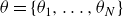 $\theta = \{\theta _1, \ldots , \theta _N \}$
, where
$\theta = \{\theta _1, \ldots , \theta _N \}$
, where
 $N$
can be very large. As such, neural networks belong to the broader family of parametric models.
$N$
can be very large. As such, neural networks belong to the broader family of parametric models.
From the early models (Rosenblatt Reference Rosenblatt1958), the core idea behind neural networks has remained: decompose the complex function
 $f_\theta$
into a composition of simple building blocks called neurons. Each neuron receives an input
$f_\theta$
into a composition of simple building blocks called neurons. Each neuron receives an input
 $x_n$
and produces an output
$x_n$
and produces an output
 $y_n$
, where
$y_n$
, where
 $x_n$
and
$x_n$
and
 $y_n$
can represent either the actual inputs or outputs of the target function
$y_n$
can represent either the actual inputs or outputs of the target function
 $f{\kern-1pt}(\boldsymbol{\cdot })$
, or intermediate values, often referred to as hidden variables.
$f{\kern-1pt}(\boldsymbol{\cdot })$
, or intermediate values, often referred to as hidden variables.
Most modern network architectures still follow the seminal principle introduced by McCulloch & Pitts (Reference McCulloch and Pitts1943), inspired by biological neurons: each artificial neuron is composed of: (i) a linear parametrised aggregation function
 $h_\theta$
, followed by (ii) a fixed nonlinear activation function
$h_\theta$
, followed by (ii) a fixed nonlinear activation function
 $\sigma$
. This leads to the fundamental equation of a neuron:
$\sigma$
. This leads to the fundamental equation of a neuron:
 \begin{align} y_n = \sigma (h_\theta (x_n)). \end{align}
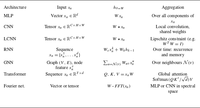
Despite its simplicity, (2.1) offers a flexible framework to construct a wide range of neural network architectures. The form of the aggregation function
 $h_\theta$
can be tailored to the input structure, as illustrated in table 1. Moreover, the choice of aggregation function directly impacts the properties of the resulting network, as further detailed in § 4.1.2. For instance, employing convolutional operations in convolutional neural networks (CNNs) allows weights sharing across the whole image, significantly reducing the number of learnable parameters (i.e. smaller
$h_\theta$
can be tailored to the input structure, as illustrated in table 1. Moreover, the choice of aggregation function directly impacts the properties of the resulting network, as further detailed in § 4.1.2. For instance, employing convolutional operations in convolutional neural networks (CNNs) allows weights sharing across the whole image, significantly reducing the number of learnable parameters (i.e. smaller
 $W$
). In addition, since convolution is translational equivariant, this symmetry naturally extends to the convolutional layers of the network.
$W$
). In addition, since convolution is translational equivariant, this symmetry naturally extends to the convolutional layers of the network.
Various well-known neural architectures, and their respective input format
 $x_n$
and associated aggregation function
$x_n$
and associated aggregation function
 $h_\theta$
parametrised by
$h_\theta$
parametrised by
 $\theta = W$
(bias is omitted for brevity). Architectures considered include the multilayer perceptron (MLP), convolutional neural network (CNN), Lipschitz-constrained neural network (LCNN), recurrent neural network (RNN) or graph neural network (GNN).
$\theta = W$
(bias is omitted for brevity). Architectures considered include the multilayer perceptron (MLP), convolutional neural network (CNN), Lipschitz-constrained neural network (LCNN), recurrent neural network (RNN) or graph neural network (GNN).

While most aggregation functions are linear, it is worth noting that attention mechanisms (Vaswany et al. Reference Vaswany, Shazeer, Parmar, Uszkoreit, Jones, Gomez and Kaiser2017) in transformer architecture (table 1) behave differently. Although the values
 $V$
are obtained through a linear transformation of the input (
$V$
are obtained through a linear transformation of the input (
 $V = x_n W_V$
), the global attention weights depend on the inputs: they are computed as
$V = x_n W_V$
), the global attention weights depend on the inputs: they are computed as
 \begin{align} W(x_n) = \text{Softmax}(QK^t/\sqrt {d}), \end{align}
where the query is
 $Q = x_n W_Q$
, the key is
$Q = x_n W_Q$
, the key is
 $K = x_n W_K$
and
$K = x_n W_K$
and
 $d$
is the dimensionality of the query/key vectors. Since both
$d$
is the dimensionality of the query/key vectors. Since both
 $Q$
and
$Q$
and
 $K$
are linear in
$K$
are linear in
 $x_n$
, the dot product
$x_n$
, the dot product
 $QK^t$
introduced a quadratic dependency of the input, resulting in a nonlinear data-dependent aggregation weights
$QK^t$
introduced a quadratic dependency of the input, resulting in a nonlinear data-dependent aggregation weights
 $W(x_n)$
. This makes attention mechanisms fundamentally different and powerful, compared with fixed or shared-weight linear aggregations like convolutions.
$W(x_n)$
. This makes attention mechanisms fundamentally different and powerful, compared with fixed or shared-weight linear aggregations like convolutions.
Once the aggregation and activation functions are chosen, several neurons can be interconnected to form a network. Neurons are typically organised into layers, where all neurons in a layer share the same inputs, but produce different outputs. These outputs then serve as inputs for the neurons in the next layer. Stacking multiple layers introduces additional nonlinearities into the model, thereby increasing its capacity to represent complex functions. When a network contains many layers, it is called a deep neural network. The way neurons are interconnected across layers defines the network architecture. Various connection patterns can be employed, such as skip connections or residual blocks, which often improve training stability and convergence. Additional modules, such as normalisation layers, or downsampling and upsampling operations can also be included to enhance performance or efficiency. Overall, the flexibility in defining both the neuron internal structure and the network architecture makes neural networks an extremely versatile framework, capable of addressing a wide range of tasks and data modalities.
2.2. Training procedure: learning is optimising
Training a neural network consists in optimising its weights
 $\theta$
to minimise a metric, often called loss function, denoted
$\theta$
to minimise a metric, often called loss function, denoted
 $\mathcal{L}(\boldsymbol{\cdot })$
. In supervised learning, this process relies on a training dataset
$\mathcal{L}(\boldsymbol{\cdot })$
. In supervised learning, this process relies on a training dataset
 $\mathcal{D}_T = \{ x^{(i)}, y^{(i)} \}_{i=1..M}$
composed of input–output pairs, where
$\mathcal{D}_T = \{ x^{(i)}, y^{(i)} \}_{i=1..M}$
composed of input–output pairs, where
 $x^{(i)}$
(respectively
$x^{(i)}$
(respectively
 $y^{(i)}$
) is the ith input (respectively target output) sample. The goal of training is therefore to find the optimal set of weights
$y^{(i)}$
) is the ith input (respectively target output) sample. The goal of training is therefore to find the optimal set of weights
 $\theta ^*$
that minimises the loss over all samples in the dataset, which can be expressed generically as
$\theta ^*$
that minimises the loss over all samples in the dataset, which can be expressed generically as
 \begin{align} \theta ^* = \text{argmin}_\theta \big [ \mathcal{L} \big ( f_\theta (x^{(i)}), y^{(i)}, \theta \big ) \big ]\quad \text{ for all } \{ x^{(i)}, y^{(i)} \} \in \mathcal{D}_T. \end{align}
Equation (2.3) provides a general and flexible formulation of the learning process, where the choice of the target definition
 $y$
and the loss function
$y$
and the loss function
 $\mathcal{L}$
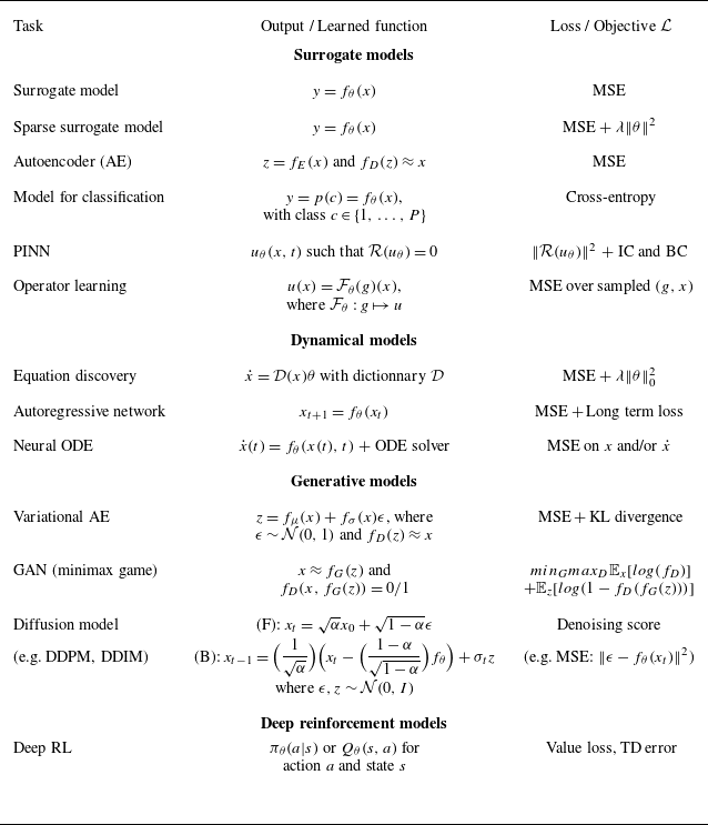
determines the type of neural network and the nature of the task it can address. Depending on these choices, one can design models for surrogate modelling, generative modelling, classification or even deep reinforcement learning (see table 2). As a simple example, a standard supervised training set-up using the mean squared error (MSE) loss is defined as
$\mathcal{L}$
determines the type of neural network and the nature of the task it can address. Depending on these choices, one can design models for surrogate modelling, generative modelling, classification or even deep reinforcement learning (see table 2). As a simple example, a standard supervised training set-up using the mean squared error (MSE) loss is defined as
 \begin{align} \mathcal{L} = \big \| f_\theta (x^{(i)}) - y^{(i)} \big \|^2. \end{align}
In contrast, incorporating L2 regularisation (also known as weight decay) modifies the objective as
 \begin{align} \mathcal{L} = \big \| f_\theta (x^{(i)}) - y^{(i)} \big \|^2 + \lambda \| \theta \|^2, \end{align}
where
 $\lambda$
is a user-defined hyperparameter controlling the strength of the regularisation term and
$\lambda$
is a user-defined hyperparameter controlling the strength of the regularisation term and
 $\| \boldsymbol{\cdot }\|$
denotes the L2 norm. Note that classical least square method and Ridge regression correspond to (2.4)–(2.5) where the function
$\| \boldsymbol{\cdot }\|$
denotes the L2 norm. Note that classical least square method and Ridge regression correspond to (2.4)–(2.5) where the function
 $f_\theta$
is linear, i.e. where the activation function is
$f_\theta$
is linear, i.e. where the activation function is
 $\sigma = Id$
.
$\sigma = Id$
.
These surrogate models trained with an MSE loss require both the input
 $x$
and the corresponding output
$x$
and the corresponding output
 $y$
to compute the reconstruction error
$y$
to compute the reconstruction error
 $\| y - f_\theta (x) \|^2$
. When the true output is unavailable, a self-supervised strategy can still be employed by training the network to reconstruct its own input, enforcing
$\| y - f_\theta (x) \|^2$
. When the true output is unavailable, a self-supervised strategy can still be employed by training the network to reconstruct its own input, enforcing
 $x \approx f_\theta (x)$
. This approach becomes useful when the reconstruction is performed through a low-dimensional latent code
$x \approx f_\theta (x)$
. This approach becomes useful when the reconstruction is performed through a low-dimensional latent code
 $z$
, which enables an efficient compression of the input representation. This task is typically achieved through an autoencoder (AE) architecture, composed of two networks: an encoder
$z$
, which enables an efficient compression of the input representation. This task is typically achieved through an autoencoder (AE) architecture, composed of two networks: an encoder
 $f_E$
that compresses the input into a latent code
$f_E$
that compresses the input into a latent code
 $z = f_E(x)$
and a decoder
$z = f_E(x)$
and a decoder
 $f_D$
that reconstructs the original sample as
$f_D$
that reconstructs the original sample as
 $x \approx f_D(z)$
. Once trained, the latent code
$x \approx f_D(z)$
. Once trained, the latent code
 $z$
can be sampled (e.g.
$z$
can be sampled (e.g.
 $z \sim \mathcal{N}(0, I)$
), turning the model into a generative network capable of producing new data. To explicitly enforce this sampling property during training, one can constrain the latent variables to follow a prescribed distribution, typically a standard Gaussian law, by minimising the Kullback–Leibler (KL) divergence between the learned distribution
$z \sim \mathcal{N}(0, I)$
), turning the model into a generative network capable of producing new data. To explicitly enforce this sampling property during training, one can constrain the latent variables to follow a prescribed distribution, typically a standard Gaussian law, by minimising the Kullback–Leibler (KL) divergence between the learned distribution
 $p(z)$
and the target prior
$p(z)$
and the target prior
 $\mathcal{N}(0, I)$
. Combining this regularisation term with the reconstruction loss yields the well-known variational autoencoder (VAE) formulation.
$\mathcal{N}(0, I)$
. Combining this regularisation term with the reconstruction loss yields the well-known variational autoencoder (VAE) formulation.
Following this idea, other techniques have been developed for enhanced generative modelling. For example, generative adversarial networks (GANs) proposed by Goodfellow et al. (Reference Goodfellow, Pouget-Abadie, Mirza, Xu, Warde-Farley, Ozair, Courville and Bengio2014) also rely on a low-dimensional latent code
 $z$
to generate synthetic samples
$z$
to generate synthetic samples
 $x \approx f_G(z)$
. In addition, a second network, the discriminator
$x \approx f_G(z)$
. In addition, a second network, the discriminator
 $f_D$
, is trained to distinguish whether an image is real (taken from the dataset) or fake (produced by
$f_D$
, is trained to distinguish whether an image is real (taken from the dataset) or fake (produced by
 $f_G$
). This set-up defines a minimax optimisation problem, in which the loss is simultaneously minimised to improve the generator
$f_G$
). This set-up defines a minimax optimisation problem, in which the loss is simultaneously minimised to improve the generator
 $f_G$
and maximised to enhance the discriminator’s ability to detect fake images. Although GANs are mathematically well posed, they are notoriously difficult to train in practice and often suffer from mode collapse, a phenomenon where the generator produces limited diversity in the generated outputs. To address these challenges, diffusion-based models (Ho et al. Reference Ho, Jain, Abbeel, Larochelle, Ranzato, Hadsell, Balcan and Lin2020; Song, Meng & Ermon Reference Song, Meng and Ermon2020) have recently emerged. In their forward process (F), random noise
$f_G$
and maximised to enhance the discriminator’s ability to detect fake images. Although GANs are mathematically well posed, they are notoriously difficult to train in practice and often suffer from mode collapse, a phenomenon where the generator produces limited diversity in the generated outputs. To address these challenges, diffusion-based models (Ho et al. Reference Ho, Jain, Abbeel, Larochelle, Ranzato, Hadsell, Balcan and Lin2020; Song, Meng & Ermon Reference Song, Meng and Ermon2020) have recently emerged. In their forward process (F), random noise
 $\epsilon$
is gradually added to an initial image
$\epsilon$
is gradually added to an initial image
 $x_0$
, generating a sequence of increasingly noisy images
$x_0$
, generating a sequence of increasingly noisy images
 $x_t$
. Since the noise
$x_t$
. Since the noise
 $\epsilon$
and the corresponding noisy image
$\epsilon$
and the corresponding noisy image
 $x_t$
are both known, the task can be formulated as a supervised learning problem, where the network is trained to predict the noise using a standard MSE loss:
$x_t$
are both known, the task can be formulated as a supervised learning problem, where the network is trained to predict the noise using a standard MSE loss:
 \begin{align} \mathcal{L} = \| \epsilon - f_\theta (x_t, t) \|^2. \end{align}
During the reverse process (B), the model starts from a pure Gaussian noise sample and progressively denoises it by subtracting the learned noise prediction
 $f_\theta$
at each step, yielding increasingly realistic reconstructions. To preserve stochasticity and allow for diversity in the generated samples, an additional noise term
$f_\theta$
at each step, yielding increasingly realistic reconstructions. To preserve stochasticity and allow for diversity in the generated samples, an additional noise term
 $\sigma _t z$
, with
$\sigma _t z$
, with
 $z \sim \mathcal{N}(0, I)$
, is injected during the backward diffusion. These generative models for physics are further detailed in § 4.6.1.
$z \sim \mathcal{N}(0, I)$
, is injected during the backward diffusion. These generative models for physics are further detailed in § 4.6.1.
Note that classification tasks also fit naturally within this general framework by predicting probability distributions rather than deterministic outputs. In such cases, the objective is to identify the most likely class
 $c$
(an integer label), which is commonly reformulated as predicting the corresponding class probabilities
$c$
(an integer label), which is commonly reformulated as predicting the corresponding class probabilities
 $p(c)$
. To properly train the network on these probabilistic targets, the loss function must therefore measure discrepancies between probability distributions rather than pointwise errors. This is precisely the role of the cross-entropy and KL divergence losses, which quantify the distance between the predicted probability distribution and the true one.
$p(c)$
. To properly train the network on these probabilistic targets, the loss function must therefore measure discrepancies between probability distributions rather than pointwise errors. This is precisely the role of the cross-entropy and KL divergence losses, which quantify the distance between the predicted probability distribution and the true one.
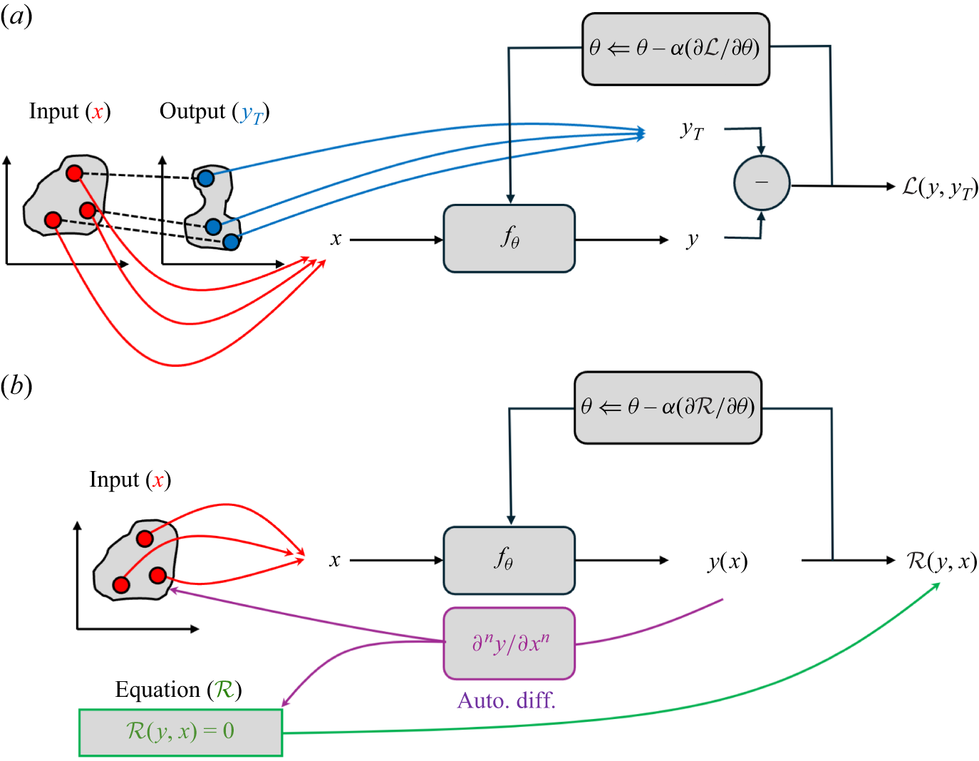
Beyond purely data-driven tasks such as classification or generative modelling, neural networks can also leverage prior physical knowledge to guide learning. In physics-informed neural networks (PINNs) proposed by Raissi et al. (Reference Raissi, Perdikaris and Karniadakis2019), for instance, the solution field
 $u_\theta (x, t)$
is parametrised by a neural network and trained by minimising the residual of the governing equations,
$u_\theta (x, t)$
is parametrised by a neural network and trained by minimising the residual of the governing equations,
 $\mathcal{R}(u_\theta (x, t))$
. This approach effectively relaxes the need for labelled data, as the network is constrained by the underlying physics. Initial (IC) and boundary (BC) conditions can be naturally incorporated into the loss function as additional terms. While PINNs focus on learning solution fields, more recent methods aim to directly learn operators that map inputs to outputs. Such operator learning approaches, including the Fourier neural operator (FNO), DeepONet and implicit neural representation (INR), are particularly useful for multi-scale or parametric problems and are discussed in detail in § 4.2.3.
$\mathcal{R}(u_\theta (x, t))$
. This approach effectively relaxes the need for labelled data, as the network is constrained by the underlying physics. Initial (IC) and boundary (BC) conditions can be naturally incorporated into the loss function as additional terms. While PINNs focus on learning solution fields, more recent methods aim to directly learn operators that map inputs to outputs. Such operator learning approaches, including the Fourier neural operator (FNO), DeepONet and implicit neural representation (INR), are particularly useful for multi-scale or parametric problems and are discussed in detail in § 4.2.3.
Finally, deep reinforcement learning (DRL), often used for optimal control of fluid flows (Verma, Novati & Koumoutsakos Reference Verma, Novati and Koumoutsakos2018; Rabault et al. Reference Rabault, Kuchta, Jensen, Réglade and Cerardi2019; Berger et al. Reference Berger, Arroyo-Ramo, Guillet, Lahire, Martin, Jardin, Rachelson and Bauerheim2024; Koumoutsakos Reference Koumoutsakos2024), can also be framed within this general neural network perspective. In DRL, a network is trained to approximate either the optimal policy
 $\pi _\theta (a | s)$
or the action-value function
$\pi _\theta (a | s)$
or the action-value function
 $Q_\theta (s, a)$
, as a function of the system state
$Q_\theta (s, a)$
, as a function of the system state
 $s$
and action
$s$
and action
 $a$
. The main challenge is that the true target is not known a priori, since it would require the knowledge of the optimal control law. Consequently, the target must be iteratively estimated during training, yielding a loss function similar to MSE, but with self-consistent updated targets instead of fixed labels. This formulation naturally fits within the general neural network framework, although it typically results in more unstable training dynamics compared with standard supervised learning.
$a$
. The main challenge is that the true target is not known a priori, since it would require the knowledge of the optimal control law. Consequently, the target must be iteratively estimated during training, yielding a loss function similar to MSE, but with self-consistent updated targets instead of fixed labels. This formulation naturally fits within the general neural network framework, although it typically results in more unstable training dynamics compared with standard supervised learning.
Beyond the task-specific formulations summarised in table 2, recent advances have introduced a new class of broadly trained models known as foundation models (Bommasani et al. Reference Bommasani2022). Typical examples are large language models (LLM) such as the well-known ChatGPT (Brown et al. Reference Brown, Larochelle, Ranzato, Hadsell, Balcan and Lin2020). Instead of optimising a network for a single objective, they are rather pretrained on massive heterogeneous datasets using self-supervised objectives, with the goal of learning general-purpose representations of data. After this large-scale pretraining, the resulting representations can be adapted to a wide variety of downstream tasks (regression, classification, generation or control), often with minimal additional training.
Overview of various neural network tasks with their associated learned function and training objectives.

In conclusion, neural networks offer a flexible and generic framework capable of tackling a wide range of complex tasks. The natural next question is how effective this framework truly is, particularly when compared with the well-established and highly optimised mathematical algorithms commonly used in computational physics, and especially in CFD. This comparison will allow the identification of key principles from classical methods that could guide neural networks to achieve comparable, or even superior, performance.
3. Effectiveness of mathematics throughout the history of science
Since Galileo Galilei, physicians intensively employ mathematics to describe natural phenomena, including gravitation, electro-magnetic fields as well as fluid mechanics among many others, exhibiting remarkable precision and generalisation capabilities. According to Feynman, ‘If you want to learn about nature, to appreciate nature, it is necessary to understand the language that she speaks in’. This statement is in line with the Galilei’s conjecture that the language of nature is mathematics. While this viewpoint implies the straightforward effectiveness of mathematics, it relies solely on Galileo’s conjecture, which cannot be demonstrated or rejected, yielding endless circular debates with no resolution in sight. Thus, let us consider another perspective, where mathematics in physics is useful because we have no choice. For instance, Kepler posed the question ‘What else can the human mind hold besides numbers and magnitudes?’. In other words, the real world is too complex and mathematics is our sole means to make this inherent complexity of nature intelligible to human understanding. Let us consider the situation where only the mathematical properties of the physical world are accessible to humans. Here, mathematics is not considered as the language of nature, but rather a tool for humans to apprehend its complexity. In that situation, physics would be effective only because its use is limited to mathematisable questions. This is evident in fields like medicine, where very few equations exist to describe the fundamental interactions between living cells or biological systems, making it less amenable to mathematical treatments. Note that mathematics are still used for specific problems, like understanding the microbial population dynamics (Quedeville Reference Quedeville2020) or the DNA replication and repair using knot theory (Robic & Jungck Reference Robic and Jungck2011), among others, including the pioneer works to create mathematical models of biological neurons, yielding the emergence of AI (McCulloch & Pitts Reference McCulloch and Pitts1943). Interestingly, this limitation had led to the early widespread adoption of AI in medical research, such as cancer detection (Tekkesin Reference Tekkesin2019) and protein discovery (Madani et al. Reference Madani2023), since no other efficient algorithm was already successful for such tasks. Nevertheless, does it imply that AI cannot play a crucial role in disciplines already massively based on mathematics, as it is the case for fluid mechanics and CFD, and more generally in computational physics? How can mathematics and AI complement each other in such domains? Can the fundamental properties of mathematics be transposed into AI to enhance both its effectiveness and adoption within the scientific community? In my opinion, these questions are rarely addressed and, therefore, this section is dedicated to explore and to answer them, at least partially.
3.1. Definitions of effectiveness
Before diving into the epistemology of mathematics, the notion of the effectiveness of a scientific method should be defined and clarified. According to Wigner (Reference Wigner1960), the effectiveness of mathematics in natural science is a miracle, out of reach of the human understanding. Nevertheless, he defined three levels of effectiveness in physics.
First, the prediction capability. As a main objective throughout history, scientific models and theories have been developed to predict behaviours of physical phenomena. In that view, a naïve definition of effectiveness is the capability of a model to predict accurately unseen behaviours, i.e. to generalise to new conditions, at least in a pre-defined range of operating points. On one hand, it is worth noting that prediction effectiveness should not be confused with the sole accuracy, but should be also related to its inherent cost to provide such a prediction. For instance, is Reynolds-averaged Navier–Stokes more or less effective than large eddy simulation (LES) or even DNS in the context of CFD? Similarly, is a linear regression model less effective than a deep neural network? Consequently, a proper metric defining the trade-off between accuracy and cost (or any measure of the complexity of a model) has to be proposed when such effectiveness is invoked. An alternative is to set an accuracy threshold and evaluate the cost of the method to obtain this user-defined accuracy (Ajuria-Illaramendi, Bauerheim & Cuenot Reference Ajuria-Illaramendi, Bauerheim and Cuenot2022). On the other hand, unseen behaviour is usually not clearly defined. This is due to the difficulty to properly construct a metric to assess how far a new behaviour is, compared with previous seen phenomena. For instance, this difficulty typically arises in very high dimension, as usually encountered with deep learning (Xia et al. Reference Xia, Xiong, Luo, Xu and Zhang2015), so that identifying ‘unseen’ data to evaluate generalisation becomes illusive. This question is attracting attention recently, in particular by finding methods to identify these out-of-distribution data (Durasov et al. Reference Durasov, Oner, Donier, Le and Fua2024; Yang et al. Reference Yang, Zhou, Li and Liu2024).
Second, the capability to provide explainable structures. Mathematics in physics is not limited to reproduce results provided by experiments, but allows us to understand the underlying mechanisms and structures encompassing, and thus explaining, multiple similar situations. It constitutes a conceptual generalisation. As an illustration, the general relativity proposed by Einstein (Reference Einstein1920) goes beyond its simple validation, such as the recent tests on the weak equivalence principle provided by the Microscope mission (Touboul Reference Touboul2022). Indeed, this theory offered to see gravitation as the curvature of the four-dimensional space–time, rather than considering it as a mere force. This epistemological rupture allowed the explanation of the previously insoluble anomaly of Mercury’s orbit, but also the description of new phenomena as surprising as gravitational lenses, black holes or gravitational waves. As a consequence, this theory goes beyond predictions, bringing also explanation, which echoes the ‘Predicting is not explaining’ written by Thom, Tsatsanis & Lisker (Reference Thom, Tsatsanis and Lisker2016). In addition, he underlined the need of unification in physics, which stipulates that explaining means reducing the large diversity of phenomena to a few general principles. It is worth noting that in this viewpoint, CFD is effective in predicting flows, but not directly to explain their behaviour: to do so, post-processing and analysis are always required. For example, while compressible CFD allows the simulation of aero-acoustic phenomena, determining the type and localisation of acoustic sources in a simulated flow still constitutes a challenge. This requires state-of-the-art post-processing, like Helmholtz’s or Doak’s decompositions, to separate acoustic perturbations from turbulent and hydrodynamic ones (D’Aniello et al. Reference D’Aniello, Gövert, Knobloch and Kissner2023). Similarly, finding the correlation between flow structures, like vortices, and quantities of interest, like lift, also necessitate the development of novel post-processing, like the force partitioning method (Menon & Mittal Reference Menon and Mittal2021), to extract meaningful information from the CFD simulations.
Third, the conceptual generative. Effectiveness can also be associated with another capability, the one called ‘generative’ by Wigner (Reference Wigner1960). This notion translates the ability of a theory, not to predict or to explain, but to fertilise novel ideas and concepts, often based on new representations. Bachelard (Reference Bachelard1936) emphasised this notion by stating that ‘mathematical information gives us more than reality; it gives us the plan of the possible; it goes beyond the actual experience of coherence’. In essence, the objective of mathematics in physics extends beyond merely providing theories consistent with experimental measurements. Rather, it provides a systematic framework that, starting from a small set of foundational principles, generates the full range of possible theories consistent with those principles. This approach allows physicists to generalise existing concepts, but also to envision novel ones, even in the absence of empirical validation or refutation (Maronne & Patras Reference Maronne and Patras2022): ‘To think about reality is to construct it mathematically’. Consider two examples from the history of scientific discoveries. On one hand, in 1846, Le Verrier predicted the existence of Neptune using only mathematical calculations. Its presence was soon confirmed by Galle’s observations. This was an impressive achievement, but this was just one more planet among those already known. On the other hand, the theoretical predictions of the Higgs boson introduced an entirely new kind of entity into physics, while providing a conceptual shift where mass is not an intrinsic property of particles. This idea was experimentally confirmed only 48 years later at the Large Hadron Collider (LHC), revealing that conceptual generative can appear prior to any prediction capabilities of a theory. It is worth noting that mathematical theories can exhibit conceptual generative without necessarily producing significant new explanations or predictions, as seen in string theory. In that case, the new physical concept serves as a source of new ideas for pure mathematics. Such theories with conceptual generative but not yet experimentally verified are often denoted as ‘tentative theories’ (Penrose Reference Penrose1990). This illustrates that no inclusion relationship exists between these three levels of effectiveness: predictive, explanatory and conceptual generative.
Nevertheless, AI for CFD remains an emerging approach and to be considered truly effective, it must consistently prove its predictive power by surpassing traditional mathematical tools. This is a prerequisite for broader adoption within the research and engineering communities. However, while AI has demonstrated superior performance in specific tasks and configurations, a major challenge remains: extending its applicability to a wider range of problems with minimal or no retraining. Interestingly, the rapid advancements in AI to achieve this objective have sparked a wave of innovative ideas, particularly in the modelling and understanding of these algorithms. In fluid mechanics, novel concepts bridging AI and CFD have emerged, showcasing its potential for conceptual generative effectiveness. Examples include physics-informed neural networks (PINNs) introduced by Raissi et al. (Reference Raissi, Perdikaris and Karniadakis2019), which approximate partial differential equation (PDE) solutions with continuous functions without relying on gradient approximations, and hybrid differentiable solvers (Um et al. Reference Um, Brand, Fei, Holl and Thuerey2020), which seamlessly integrate AI with classical numerical methods. Thus, the next crucial challenge for AI lies in explanatory effectiveness. First, AI models and training strategies must be interpretable, providing clear guidelines for practical implementation and facilitating adoption in research and engineering. Second, beyond just predictive accuracy, AI systems should be capable of understanding and explaining the underlying physics, similar to the ‘agent of understanding’ proposed by Krenn et al. (Reference Krenn2022), a challenge rarely addressed in the literature. While AI has shown promise in identifying complex nonlinear physical phenomena, its ability to provide physical insights remains limited, in particular on unknown and complex problems. This lack of interpretability represents a key area for future improvement, and I believe this is an essential step for AI to evolve into a reliable tool for scientific discovery and engineering applications.
That being said, note that Wigner (Reference Wigner1960) also insists on the fact that a new formalism, tool or concept is rarely directly applicable in the domain for which it was thought. As a consequence, evaluating the effectiveness of a theory a priori has no significant meaning or, at the very least, necessitates a careful consideration. This is why the following sections do not investigate the effectiveness of mathematics and AI based on their respective current results, but rather on their epistemological potential. Let us begin by delving into the origins of mathematical effectiveness to extract its foundational principles.
3.2. A reasonable explanation of the effectiveness of mathematics
3.2.1. Symmetries and invariants
Lambert (Reference Lambert1997) has examined the possible reasons behind the effectiveness in mathematics in his book ‘Is the efficiency of mathematics unreasonable?’, inspiring the title of this very subsection. Within this work, he explores various philosophical theories, such as Pythagoreanism, Platonism, empiricism etc. intended to explain the effectiveness of mathematics and, in general, to every scientific methods. Among them, he mentioned formalism, which stipulates that mathematics is effective because it relies on symbols and rules to manipulate them. Nevertheless, Lambert (Reference Lambert1997) argues that this point of view can explain the effectiveness of mathematics only as a kind of miracle, as it is difficult to see how a ‘game’ governed solely by constraints of internal coherence could correspond to a reality external to thought, such as physical phenomena. However, this theory gave birth to relationism, which considers mathematics as the formalised representation of all possible conceptual relationships, including numerical ones. For instance, according to Bohr (Reference Bohr1958), ‘we shall not consider pure mathematics as a separate branch of knowledge, but rather as a refinement of general language, supplementing it with appropriate tools to represent relations for which ordinary verbal expression is imprecise or cumbersome’. Here, mathematics is not just a language with symbols and rules, but serves as a means of formally translating and elucidating the relationships between concepts. This might explain why physics is well mathematised, since most results can be expressed through structured relationships between the fundamental quantities of the system, structures that mathematics can faithfully capture and elaborate. According to Vandamme (Reference Vandamme1976), ‘The knowledge in general, and even more so the scientific knowledge, is characterised by its structures’. Nevertheless, it is worth noting that not all relationships are useful. Corry (Reference Corry1996) notes that mathematicians are not interested in cataloguing all possible structures, but rather to investigate ones that possess rich invariants. This is consistent with physics, where an ‘element of reality’ cannot be described properly without recourse to invariants preserved under the symmetries of the system. This need of invariance is motivated by our partial observation of reality that requires invariants to conclude without exhaustive observations, which is often impractical or cumbersome. In other words, reality in physics must be robust to a change of point of view. This is exactly what research in physics is doing, but more generally how humans and animals perceive the surrounding world. For instance, Florack et al. (Reference Florack, Romeny, Koenderink and Viergever1994) and Lindeberg (Reference Lindeberg2013) have demonstrated that human vision and cognitive functions rely on some invariants and symmetries: ‘It is apparently the case that, at least up to some approximation, many visual tasks can be solved on the basis of such invariants only. This observation should affect the way computer-vision and image-analysis tasks are handled as well’ (Florack et al. Reference Florack, Romeny, Koenderink and Viergever1994).
Modern science, and mathematics, now heavily rely on the study of symmetry, as illustrated by Anderson (Reference Anderson1972) who noted that ‘it is only slightly overstating the case to say that physics is the study of symmetry’. Early on, Curie (Reference Curie1984) proposed his principle of symmetry, based on ideas from F. Neumann and B. Minnigerode, where ‘the symmetries of the causes are to be found in the effects’. This highlights the profound relevance of symmetries to understand the surrounding world. Interestingly, symmetries in physics are intricately related to invariants, i.e. conserved quantities, also known as first integrals, as elegantly elucidated by Noether’s theorem (Noether Reference Noether1918). As an example, rotational symmetry yields the conservation of angular momentum, and invariance under a translation in time leads to the conservation of energy. Moreover, symmetries and invariances are much more intricate and influential in modern physics.
In the realm of fluid mechanics, the rigorous investigation of symmetry and invariance has also been studied for a long time. For instance, Golubitsky & Stewart (Reference Golubitsky and Stewart1986) studied the specific symmetries acting on the stability of Taylor–Couette flows. They demonstrate that symmetries inherent in bifurcating systems have a strong influence on their behaviour, which motivates their study. The effect of symmetries on flow instability has been recently revisited by Sierra-Ausin, Fabre & Knobloch (Reference Sierra-Ausin, Fabre and Knobloch2024), focusing on the
 $O(2)$
symmetry applied to wake instability. Similarly, combustion instabilities in annular combustion chambers are governed by the azimuthal symmetry. When this symmetry is broken because of different flame types (Bauerheim et al. Reference Bauerheim, Salas, Nicoud and Poinsot2014b
), azimuthal mean flow (Bauerheim et al. Reference Bauerheim, Cazalens and Poinsot2014a
) or stochasticity (Bauerheim et al. Reference Bauerheim, Ndiaye, Constantine, Moreau and Nicoud2016a
), modal splitting occurs which affects the whole stability of the system. Recent works in thermoacoustics still involves this notion of symmetry breaking (Aguilar et al. Reference Aguilar, Dawson, Schuller, Durox, Prieur and Candel2021; Faure-Beaulieu et al. Reference Faure-Beaulieu, Indlekofer, Dawson and Noiray2021). Symmetries have also been exploited in fluid mechanics to build turbulence models. Indeed, Grebenev & Oberlack (Reference Grebenev and Oberlack2007) and Fakhar et al. (Reference Fakhar, Hayat, Yi and Zhao2009) studied the symmetry of the incompressible Navier–Stokes equations (Cantwell Reference Cantwell1978). Based on these symmetries, Razafindralandy, Hamdouni & Oberlack (Reference Razafindralandy, Hamdouni and Oberlack2007) and later Sayed et al. (Reference Sayed, Hamdouni, Liberge and Razafindralandy2010) derived new turbulence modelling which preserve those symmetries. They also analysed the existing turbulence models available at that time, including the Smagorinsky model (Smagorinsky Reference Smagorinsky1963), showing that only its dynamic version (Germano et al. Reference Germano, Piomelli, Moin and Cabot1991) allows symmetry preservation.
$O(2)$
symmetry applied to wake instability. Similarly, combustion instabilities in annular combustion chambers are governed by the azimuthal symmetry. When this symmetry is broken because of different flame types (Bauerheim et al. Reference Bauerheim, Salas, Nicoud and Poinsot2014b
), azimuthal mean flow (Bauerheim et al. Reference Bauerheim, Cazalens and Poinsot2014a
) or stochasticity (Bauerheim et al. Reference Bauerheim, Ndiaye, Constantine, Moreau and Nicoud2016a
), modal splitting occurs which affects the whole stability of the system. Recent works in thermoacoustics still involves this notion of symmetry breaking (Aguilar et al. Reference Aguilar, Dawson, Schuller, Durox, Prieur and Candel2021; Faure-Beaulieu et al. Reference Faure-Beaulieu, Indlekofer, Dawson and Noiray2021). Symmetries have also been exploited in fluid mechanics to build turbulence models. Indeed, Grebenev & Oberlack (Reference Grebenev and Oberlack2007) and Fakhar et al. (Reference Fakhar, Hayat, Yi and Zhao2009) studied the symmetry of the incompressible Navier–Stokes equations (Cantwell Reference Cantwell1978). Based on these symmetries, Razafindralandy, Hamdouni & Oberlack (Reference Razafindralandy, Hamdouni and Oberlack2007) and later Sayed et al. (Reference Sayed, Hamdouni, Liberge and Razafindralandy2010) derived new turbulence modelling which preserve those symmetries. They also analysed the existing turbulence models available at that time, including the Smagorinsky model (Smagorinsky Reference Smagorinsky1963), showing that only its dynamic version (Germano et al. Reference Germano, Piomelli, Moin and Cabot1991) allows symmetry preservation.
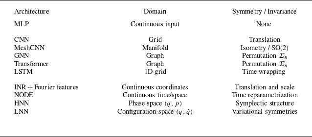
These examples reveal the uncanny effectiveness of mathematics because of symmetry and invariance, highlighting its capacity to shape our understanding of reality while existing purely within the realm of abstract ideas. This fundamental concept of symmetries and invariance is also embedded in the very construction of modern AI methods for classification and regression tasks (Gens & Domingos Reference Gens and Domingos2014; Weiler et al. Reference Weiler, Geiger, Welling, Boomsma and Cohen2018; Weiler & Cesa Reference Weiler and Cesa2019; Wang, Walters & Yu Reference Wang, Walters and Yu2021). Typical examples are CNN built upon the translation equivariance principle or graph networks based on permutation invariance. Recently, the community devoted to AI for science has been exploring the necessity of incorporating symmetries or structures directly into neural network architectures (Önder & Liu Reference Önder and Liu2023; Otto et al. Reference Otto, Zolman, Kutz and Brunton2023), not only as a design principle, but also to align with the intrinsic demands of science, which fundamentally relies on these principles. Similarly to the Erlangen programme proposed by F. Klein in 1972 to unify geometry as the study of invariants or symmetries using the language of group theory, a recent objective in AI is to unify the various network architectures into a general framework, known as geometric deep learning, based also on symmetries or invariants (Bronstein et al. Reference Bronstein, Bruna, Cohen and Velickovic2021). As a consequence, symmetry and invariants constitute the first pillar to make AI effective in CFD, as further discussed technically in § 4.1.
3.2.2. Scale separation
Furthermore, while investigating invariants for image recognition, Florack et al. (Reference Florack, Romeny, Koenderink and Viergever1992) also emphasised the scale dependence of these invariants. This notion of scale is crucial in physics, where the physical laws governing complex systems exhibit a sort of separation between the various levels of structures associated with spatial and temporal scales. For instance, while the classical Euclidean space is intuitive at spatial scales we encounter in our everyday life, this framework fails to explain phenomena at very low (quantum mechanics) and very large (gravitation) scales. Einstein (Reference Einstein1920) challenged this view by introducing the concept of curved space–time, effective at large scales, but still failing to explain the transition between the continuous world we experience and the quantised energy realm of quantum mechanics. Similarly in fluid mechanics, working at the macroscopic (Navier–Stokes equations) or mesoscopic (lattice Boltzmann method) scales does not require a detailed knowledge of the fine microscopic scales, such as the interactions between the fundamental particles. This scale separation, when available, allows dedicated physical analyses and methodologies to be performed, introducing its own abstraction. For instance, the notion of pressure at the macroscopic scale in a fluid is intuitive, while being much more complex, or even meaningless, at much lower scales.
These considerations are essential not only in physics, but also in the development of AI, as well as across a broad spectrum of disciplines, including sociology, history etc. This idea aligns closely with the epistemological perspective emphasised by Bachelard (Reference Bachelard1938), who considered that the main challenge of science is to push humans beyond their intuitive sense of scale. Additionally, Simondon (Reference Simondon1970) named scale rupture this transition between ordinary scales, where familiar schemes like particles or Euclidean space remain valid, and the extreme scales studied by quantum mechanics and astrophysics, where these schemes inherited from ordinary perception are no longer adequate. It suggests that the effectiveness of mathematics in physics derives from its ability to conceptualise and study phenomena occurring at very different scales compared with those the researcher, as a human being, is used to in a daily-life.
This principle is fundamental in CFD, where applications span an enormous range of scales, from microscopic flows around biological cells (O’Connor et al. Reference O’Connor, Day, Mandal and Revell2016) to astrophysical phenomena, such as supernova-induced turbulence and other large-scale flows in the universe (Müller Reference Müller2020). Early on, engineers and researchers recognised the necessity of classifying these flows based on characteristic non-dimensional parameters, such as the Reynolds or Mach numbers, among others. It is well established that flow behaviour changes drastically as these parameters vary, leading to the emergence of complex phenomena like shock waves or turbulence. These flow regimes can be highly localised, coexist within the same system, interact nonlinearly or even exhibit fractal characteristics (Meneveau & Sreenivasan Reference Meneveau and Sreenivasan1987), making them inherently multi-scale and challenging to capture and analyse.
Consequently, scale separation is central to many advancements in fluid mechanics. For instance, separation between the slowly varying large-scale perturbations from the rapidly varying small-scale of the flow is essential to derive a simplified effective description of the dynamics at large scales, and justify the concept of eddy viscosity (Dubrulle & Frisch Reference Dubrulle and Frisch1991). Similar multiple scale approaches are employed by Ovenden (Reference Ovenden2005) to model sound transmission through a slowly varying duct of arbitrary cross-section, by Faure-Beaulieu & Noiray (Reference Faure-Beaulieu and Noiray2022) to extract the dynamics of the slow-flow variables in an annular thermo-acoustic system, and by Magri et al. (Reference Magri, See, Tammisola, Ihme and Juniper2016) to formulate a set of equations in the low-Mach number limit for linear stability analysis.
Moreover, this multi-scale character of fluid flows lies at the core of many challenges in CFD. To address these, high-order numerical schemes (Bassi & Rebay Reference Bassi and Rebay1997; Nicoud Reference Nicoud2004) and lattice Boltzmann methods (LBMs) (Marié et al. Reference Marié, Ricot and Sagaut2009; Coratger et al. Reference Coratger, Farag, Zhao, Boivin and Sagaut2021) have been developed, specifically to preserve the propagation of fine-scale turbulent structures over long distances and to efficiently capture interactions across a wide range of scales. Similarly, identifying regions with extreme length scales, such as thin shock waves, flames or boundary layers, has led to the development of specialised numerical treatments (Colin et al. Reference Colin, Ducros, Veynante and Poinsot2000; Nicoud et al. Reference Nicoud, Baggett, Moin and Cabot2001). The critical role of scales in CFD is further highlighted by the widespread use of post-processing techniques, such as Fourier and wavelet transforms (Grizzi & Camussi Reference Grizzi and Camussi2012), proper orthogonal decomposition (POD), and other spectral analysis tools. These methods help to extract spatial and temporal scales where energy is generated or dissipated, providing deeper insight into the underlying flow physics.
This inherent multi-scale nature of fluid flows presents a significant challenge for AI, which is not initially specifically designed to handle such drastic scale separation with order of magnitudes. A clear example lies in denoising filters (Pratt Reference Pratt1972), used in some generative models, which often treat high-frequency components as noise and discard them (e.g. Wiener’s filter). In CFD, however, small-scale structures play a crucial role in accurately capturing overall flow behaviour and cannot simply be removed. Recognising this limitation, recent research has increasingly focused on equipping deep networks with multi-scale (Nabian Reference Nabian2014; Mathieu, Couprie & LeCun Reference Mathieu, Couprie and LeCun2016) and multi-resolution (Catalani et al. Reference Catalani, Agarwal, Bertrand, Tost, Bauerheim and Morlier2024; Cheng et al. Reference Cheng, Morel, Allys, Ménard and Mallat2024) capabilities, particularly for flow applications. These advancements open new avenues for improving deep learning methods in fluid mechanics by enforcing specialised treatments at different scales, as further discussed in § 4.2.
3.2.3. Sparsity
Pertaining directly to the second form of effectiveness as defined by Wigner (Reference Wigner1960), i.e. the capability to provide explainable structures, mathematics is based on concise equations (sparsity), facilitating explicability: sparsity requires abstraction, generating a semantics for physics. Semantics refers to the branch of linguistics and logic concerned with meaning. Sparsity and parsimony, as suggested by William of Occam, are of true interest since all models are wrong: ‘Pluralitas non est ponenda sine necessitate’ (Plurality is not to be posited without necessity). Among models with equivalent accuracy, the most effective are those that are sparse. For instance, the compactness of the expressions describing the Navier–Stokes equations is truly remarkable when considering the numerous physical fluid phenomena they govern: these applications range from the dynamics of blood circulation within the human heart (Chnafa et al. Reference Chnafa, Mendez, Moreno and Nicoud2015) to the airflow patterns around an aircraft, and even extend to the turbulent storms on Jupiter or the cataclysmic events of supernovae (Müller Reference Müller2020). How feasible are such compact expressions encapsulating so much physics? Occam’s razor suggests that sparsity is at the root of explicability, but nothing yet allows us to justify that these expressions will be so general and so effective in physics. This fundamental concept of sparsity is central to many approaches in recent AI for physics, such as discovering physical laws by neural networks. This is often achieved through sparsity-promoting algorithms (Brunton et al. Reference Brunton, Proctor and Kutz2016a , Reference Brunton, Proctor and Kutzb ; Silva et al. Reference Silva, Higdon, Brunton and Kutz2020) allowing to focus the explainability of the model in a few terms, and hence be more general by construction.
This explainability induced by sparsity can be illustrated with one remarkable example: the evolution of Maxwell’s equations. Initially, Maxwell (Reference Maxwell1861) formulated a set of
 $20$
equations to describe the behaviour of electric and magnetic fields. The quest for sparsity and elegance in Maxwell’s equations culminated in the realisation that the equations could be unified and simplified through the introduction of vector and tensor calculus. This reformulation has lead to a compact set of the four well-known equations, which simplifies interpretability through the divergence and curl operators, and manipulation such as deriving Poynting’s theorem for the energy conservation. However, electric (
$20$
equations to describe the behaviour of electric and magnetic fields. The quest for sparsity and elegance in Maxwell’s equations culminated in the realisation that the equations could be unified and simplified through the introduction of vector and tensor calculus. This reformulation has lead to a compact set of the four well-known equations, which simplifies interpretability through the divergence and curl operators, and manipulation such as deriving Poynting’s theorem for the energy conservation. However, electric (
 $\boldsymbol E$
) and magnetic (
$\boldsymbol E$
) and magnetic (
 $\boldsymbol B$
) fields still appear as separate entities, while in fact they can be unified into the same compact theory. This paradigm shift occurred when the equations were again reformulated, but now using the language of differential geometry. This leads to only two compact equations, where the electric and magnetic fields appear as components of a single electromagnetic tensor (
$\boldsymbol B$
) fields still appear as separate entities, while in fact they can be unified into the same compact theory. This paradigm shift occurred when the equations were again reformulated, but now using the language of differential geometry. This leads to only two compact equations, where the electric and magnetic fields appear as components of a single electromagnetic tensor (
 $F_{\mu \nu }$
), where
$F_{\mu \nu }$
), where
 $F_{0 i} = -E_i/c$
and
$F_{0 i} = -E_i/c$
and
 $F_{\textit{ij}} =- \epsilon _{\textit{ijk}} B_k$
. This unification of electric and magnetic fields is only possible because space and time are themselves combined into a single four-dimensional space–time, so that this sparse formalism naturally incorporates the principles of relativity. Beyond its compactness and elegance, this tensorial representation makes the fundamental Lorentz invariants of the electromagnetic field emerging directly from simple tensor contractions, highlighting the deep geometric structure underlying electromagnetism.
$F_{\textit{ij}} =- \epsilon _{\textit{ijk}} B_k$
. This unification of electric and magnetic fields is only possible because space and time are themselves combined into a single four-dimensional space–time, so that this sparse formalism naturally incorporates the principles of relativity. Beyond its compactness and elegance, this tensorial representation makes the fundamental Lorentz invariants of the electromagnetic field emerging directly from simple tensor contractions, highlighting the deep geometric structure underlying electromagnetism.
Similar illustrations of sparsity also arise in fluid dynamics, for instance, from the Boltzmann equation. Instead of solving directly the full set of nonlinear Navier–Stokes equations for mass, momentum and energy conservation, LBM reformulates fluid dynamics in terms of a single mesoscopic transport equation for the particle distribution function
 $F(x, t, v)$
. This sparse formulation makes conservation laws not imposed explicitly, but emerging solely from the moments of this distribution function. This is governed by the symmetries of the velocity space that ensures that only a handful of velocity moments are conserved, while the rest decay. This explains why mass, momentum and energy are the universal conservation laws in fluid flows. In addition, while the velocity space is continuous, its discretisation into a small set of representative velocities (e.g. D2Q9, D3Q19) is sufficient to preserve the essential hydrodynamic moments. This reduction transforms the complexity of the full PDE system into a simple stream-and-collide process, which is computationally effective. In this way, sparsity provides: (i) a compact representation; (ii) a clear physical interpretation; and (iii) a computational effective method.
$F(x, t, v)$
. This sparse formulation makes conservation laws not imposed explicitly, but emerging solely from the moments of this distribution function. This is governed by the symmetries of the velocity space that ensures that only a handful of velocity moments are conserved, while the rest decay. This explains why mass, momentum and energy are the universal conservation laws in fluid flows. In addition, while the velocity space is continuous, its discretisation into a small set of representative velocities (e.g. D2Q9, D3Q19) is sufficient to preserve the essential hydrodynamic moments. This reduction transforms the complexity of the full PDE system into a simple stream-and-collide process, which is computationally effective. In this way, sparsity provides: (i) a compact representation; (ii) a clear physical interpretation; and (iii) a computational effective method.
Another example of sparsity is provided by turbulence modelling. While DNS resolves all turbulent scales, a task that rapidly becomes intractable at high Reynolds numbers, RANS circumvents this by replacing the fluctuating motions with the Reynolds stress tensor, which contains only six independent unknowns. On one hand, Reynolds stress models (RSMs) solve transport equations for each component, offering high fidelity but little interpretability. On the other hand, eddy-viscosity models collapse the entire tensor to a single scalar coefficient, capturing turbulence as an effective viscosity. Despite its simplicity, it provides valuable physical insight by revealing turbulence’s essential role as a mechanism for momentum diffusion and enhanced mixing.
As a consequence, much like the compact form of Maxwell’s equations revealed the underlying structure of electromagnetism, sparse formulations and models of fluid motion provide deeper physical insight by exposing the fundamental role of key quantities in organising flow behaviour. In other words, sparsity promotes explicability. While sparsity often requires new assumptions, sometimes at the expense of predictive accuracy, these models typically retain a remarkable degree of expressive power despite being very low-parametric. However, what about the whole CFD pipeline? In practice, CFD employs high-dimensional inputs such as meshes, yielding algorithms that are not sparse in a formal sense, but nevertheless remain interpretable. I argue this interpretability arises in part because CFD is not monolithic: it is built from an aggregation of models and numerical schemes, each designed for specific objectives (e.g. turbulence closure, discretisation, boundary conditions). Such modularity allows a ‘divide and conquer’ strategy when diagnosing errors, debugging or analysing sensitivities of particular components of the modelling chain. This notion is referred as decomposability by Lipton (Reference Lipton2016), where ‘each part of the model […] admits an intuitive explanation’. In contrast, modern deep learning models tend to be monolithic, highly over-parametrised and opaque: predictive success is achieved only through massive parametrisation, but with interpretability being sacrificed (Doshi-Velez & Kim Reference Doshi-Velez and Kim2017). It highlights that the pursuit of sparsity in AI may involve trade-offs distinct from those in traditional mathematical tools. This also suggests that, while sparsity is indeed a critical pillar of effectiveness in scientific modelling, it may not be sufficient on its own: not all sparse methods are necessarily either effective or explicable, as further discussed in the AI context in § 4.3.
3.2.4. Semantic significance
In science, explicability is crucial, as it constitutes a necessary condition for constructive critical thinking. However, critical thinking can only be exercised in relation to an informed opinion, exhibiting the path and reasoning behind it. This process is often slower and more laborious than the rapid predictions of AI models. Yet, would we be willing to adhere to a result or a decision produced by an unexplainable AI, either in biology and medicine, but also in engineering? Maybe if the gap between AI and humans is substantial. This difference between slow reasoning and ultrafast predictions is characteristic of the distinction between conscious reasoning versus intuition, where the latter is ‘the ability to acquire knowledge, without recourse to conscious reasoning or needing an explanation’ (Patterson & Eggleston Reference Patterson and Eggleston2017).
A similar distinction is often invoked in artificial intelligence: on one hand, symbolic learning methods attempt to mimic conscious reasoning by manipulating explicit rules, logical relations or symbolic representations; on the other hand, statistical learning methods, such as neural networks, rely on detecting patterns in large datasets to provide rapid predictions without explicit reasoning. Mathematics aligns closely with the symbolic side, where logic and reasoning are the angular stones. In the realm of mathematics, we want to reason in an argumentative way to uncover truths. Therefore, mathematicians not only construct reality, but the mathematical notions created directly speak to reason (Bachelard Reference Bachelard1934). This forces mathematics, and thus physics, to be more than just a language with syntax, but also to possess semantics, where the structures and the relationships between mathematical objects are essential: ‘The knowledge, indeed, does not consist in a mere collection of data. On the contrary, it is well known that something can be considered as a data precisely thanks to its relationships with the structure, more or less abstract, of knowledge’ (Vandamme Reference Vandamme1976). In this context, semantics allows the reduction of information to manageable quantities with underlying structure and relationships, presented in a format or symbols (i.e. using the syntax) which facilitates their evaluations. This is precisely what mathematics accomplishes.
A typical example of semantic significance emerges in the construction of the various mathematical sets of real numbers (
 $\mathbb{R}$
), complex numbers (
$\mathbb{R}$
), complex numbers (
 $\mathbb{C}$
) and quaternions (
$\mathbb{C}$
) and quaternions (
 $\mathbb{H}$
). Consider the case of a real squared number being negative, which has no meaning in
$\mathbb{H}$
). Consider the case of a real squared number being negative, which has no meaning in
 $\mathbb{R}$
. By expanding our realm of exploration to include not only
$\mathbb{R}$
. By expanding our realm of exploration to include not only
 $\mathbb{R}$
, but also a new set
$\mathbb{R}$
, but also a new set
 $\mathbb{C}$
, we invent a new concept (‘i’, the pure imaginary number), which restores the validity of the initial proposition. However, what does this extension bring in terms of semantics? Is the transition from
$\mathbb{C}$
, we invent a new concept (‘i’, the pure imaginary number), which restores the validity of the initial proposition. However, what does this extension bring in terms of semantics? Is the transition from
 $\mathbb{R}$
to
$\mathbb{R}$
to
 $\mathbb{C}$
merely an artefact to enforce the validity of otherwise meaningless expressions or does
$\mathbb{C}$
merely an artefact to enforce the validity of otherwise meaningless expressions or does
 $\mathbb{C}$
introduce a new layer of meaning? Additionally, critically, does this meaningful transition only exist as an abstract idea or does it translate into tangible objects when analysing physical phenomena? To answer these questions, we can observed that expanding these sets inevitably alters their underlying syntactic rules. For instance,
$\mathbb{C}$
introduce a new layer of meaning? Additionally, critically, does this meaningful transition only exist as an abstract idea or does it translate into tangible objects when analysing physical phenomena? To answer these questions, we can observed that expanding these sets inevitably alters their underlying syntactic rules. For instance,
 $\mathbb{R}$
is a complete ordered field, whereas in
$\mathbb{R}$
is a complete ordered field, whereas in
 $\mathbb{C}$
, we lose ordering and in
$\mathbb{C}$
, we lose ordering and in
 $\mathbb{H}$
, commutativity. These syntactic rules, i.e. constraints governing how mathematical operations are performed, are central to the structure of these sets (Matsumoto & Nakai Reference Matsumoto and Nakai2023), which yields profound semantics much broader than their initial simple definitions. Indeed, each set provides a model for mathematical and physical systems where analogous rules are present or absent. Rotations offer a relevant example: while rotations in two dimensions are commutative, those in three dimensions are not. Consequently, unitary complex numbers can represent two-dimensional (2-D) rotations, and unitary quaternions rotations in three dimensions, since possessing the same structure. This connection between these sets and physical rotations can be formalised through the more general Lie theory, where complex numbers naturally encode planar rotations, while quaternions provide the algebraic structure underlying three-dimensional (3-D) rotations. In other words, syntactic rules and semantics are intertwined. This interconnection stems from the ability of mathematics to provide structures and relationships among diverse objects, either abstract entities as in pure mathematics (e.g. set of numbers) or tangible entities as in physics (e.g. rotations). These mathematical structures serve as a bridge between abstract ideas and real-world physical phenomena, thereby generating profound semantics to mathematics.
$\mathbb{H}$
, commutativity. These syntactic rules, i.e. constraints governing how mathematical operations are performed, are central to the structure of these sets (Matsumoto & Nakai Reference Matsumoto and Nakai2023), which yields profound semantics much broader than their initial simple definitions. Indeed, each set provides a model for mathematical and physical systems where analogous rules are present or absent. Rotations offer a relevant example: while rotations in two dimensions are commutative, those in three dimensions are not. Consequently, unitary complex numbers can represent two-dimensional (2-D) rotations, and unitary quaternions rotations in three dimensions, since possessing the same structure. This connection between these sets and physical rotations can be formalised through the more general Lie theory, where complex numbers naturally encode planar rotations, while quaternions provide the algebraic structure underlying three-dimensional (3-D) rotations. In other words, syntactic rules and semantics are intertwined. This interconnection stems from the ability of mathematics to provide structures and relationships among diverse objects, either abstract entities as in pure mathematics (e.g. set of numbers) or tangible entities as in physics (e.g. rotations). These mathematical structures serve as a bridge between abstract ideas and real-world physical phenomena, thereby generating profound semantics to mathematics.
As a result, semantics extends beyond the mere need for explainability. Incorporating semantics into a model introduces an inherent structure and sparsity, which in turn reduces computational costs, minimises data requirements, enhances generalisation and fosters greater acceptance within the scientific community. While symbolic AI methods naturally embed such structured reasoning, the current trend remains largely driven by statistical learning approaches, especially deep neural networks. This divergence raises fundamental questions about the future direction of AI in CFD. Should we continue relying solely on data-driven techniques or should we advocate for a stronger integration of symbolic AI? Given that symbolic methods also face significant challenges in tackling real-world problems, could hybrid approaches mixing symbolic AI and deep networks provide a viable alternative for CFD? Addressing these questions requires a deeper reflection on the practical means of embedding semantic structures within modern deep learning frameworks, further discussed in § 4.4.
3.2.5. Four pillars of effectiveness (PoEs)
As a summary, the effectiveness of mathematics in physics can be attributed to four main aspects, hereafter named the ‘four pillars of effectiveness’ (PoEs): (i) symmetries providing internal structures to equations; (ii) scales separation, allowing a specific treatment of the physics for each scale and their interactions; (iii) sparsity, which promotes explicability; and finally (iv) semantic significance, which gives mathematics not a purely grammatical structure, but also a meaning, facilitating abstraction and reasoning. Those aspects will be further analysed in the specific context of the development of artificial methods for CFD, which also applies more generally to computational physics.
Yet, as claimed by Jebeile (Reference Jebeile2024), the actual usability of a model is not determined solely by its accuracy or effectiveness, but also depends on its credibility, which is its ability to earn trust and foster adoption within a community. In mathematics, credibility is inherently tied to rigour and logical proof, but in AI, credibility is contingent: it depends on empirical validation, the reliability and trust in data, and the interpretability of models. For example, Levins (Reference Levins1966) argued that credibility can emerge from the ‘robustness across models’, where consistent conclusions drawn from an ensemble of different models provide confidence to shared results, an idea closely connected with epistemic uncertainties. Furthermore, Simon (Reference Simon1962, Reference Simon1969) emphasised near-decomposability and hierarchical organisation in the study of complex systems, arguing that modular structures enhance both tractability and interpretability. This insight has more recently been explored by Jebeile (Reference Jebeile2024), who mentioned that decomposability plays a key role in establishing the credibility of scientific models. This suggests that beyond the proposed PoEs, AI for CFD may also require explicit safeguards of credibility, not as a condition for effectiveness itself, but as a prerequisite for its widespread use. This fifth pillar will be further discussed in § 4.5.
4. Routes towards effective AI in CFD
Artificial Intelligence has become a transformative tool in CFD, introducing innovative strategies to address the complex, multi-scale, nonlinear challenges inherent in fluid flows. From cutting-edge neural network architectures to hybrid AI–physics models, AI demonstrates the potential to complement, or even surpass, traditional numerical methods across various applications. This comprehensive review explores key research directions at the intersection of AI and CFD, focusing on the unique challenges posed by fluid dynamics and how AI might overcome them. In particular, it investigates whether AI can implement the four pillars of mathematical effectiveness outlined in § 3.2, which are foundational to the success of mathematics in physics. These principles may provide a roadmap for endowing AI with the qualities that make mathematics so effective in modelling physical systems, in addition to a fifth pillar empowering credibility to these AI models, facilitating their widespread use.
(a) Classical network, where training data
 $(x, y_T)$
are sampled and fed to a parametrised function
$(x, y_T)$
are sampled and fed to a parametrised function
 $f_\theta$
. Training is achieved by measuring a loss function
$f_\theta$
. Training is achieved by measuring a loss function
 $\mathcal{L}$
between the prediction (
$\mathcal{L}$
between the prediction (
 $y$
) and the target (
$y$
) and the target (
 $y_T$
). Network’s weights
$y_T$
). Network’s weights
 $\theta$
are updated by a back-propagation algorithm and gradient descent methods. (b) PINN employs an equation
$\theta$
are updated by a back-propagation algorithm and gradient descent methods. (b) PINN employs an equation
 $\mathcal{R}(y, x) = 0$
. Training is achieved by computing the residual
$\mathcal{R}(y, x) = 0$
. Training is achieved by computing the residual
 $\mathcal{R}$
of the physical equation from the predictions
$\mathcal{R}$
of the physical equation from the predictions
 $y(x)$
. To do so, partial derivatives
$y(x)$
. To do so, partial derivatives
 $ {\partial ^n y}/{\partial x^n}$
are computed by automatic differentiation. Network’s weights are updated using the residual
$ {\partial ^n y}/{\partial x^n}$
are computed by automatic differentiation. Network’s weights are updated using the residual
 $\mathcal{R}$
as physical-based loss function. Since
$\mathcal{R}$
as physical-based loss function. Since
 $f_\theta$
is a continuous function of
$f_\theta$
is a continuous function of
 $x$
, the output
$x$
, the output
 $y(x)$
is theoretically continuous in space and time (infinite resolution).
$y(x)$
is theoretically continuous in space and time (infinite resolution).

In this section, I explore several pathways towards the development of effective AI for physics, each deeply rooted in the foundational pillars established in § 3.2. First, I review in § 4.1 how the various architectures of deep networks incorporate the first PoE, namely symmetry and invariance, and discuss how their internal structures can be constrained to reflect physical conservation laws. Second, I analyse in § 4.2 how scale separation (PoE-ii) is integrated through the design of multi-scale networks (§ 4.2.3), which optimise both computational and representational efficiency, as well as through the use of multi-fidelity data (§ 4.2.4), which enhance accuracy and robustness by combining sources from heterogeneous scales. Third, I argue in § 4.3 that sparsity (PoE-iii) plays a critical role in AI approaches, particularly for equation discovery and inverse problems. Fourth, I investigate in § 4.4 how recent approaches explicitly embed semantics into AI systems. Beyond these four pillars, I also address in § 4.5 the issue of credibility, understood as a prerequisite for the widespread adoption of AI in the fluid community. This involves the development of robust methods capable of quantifying uncertainty, allowing a first introduction of doubts into learning algorithms. Finally, while generative and foundation models appear at first to diverge from these PoEs, they may ultimately redefine them (§ 4.6). These models learn semantics and internal structure through specific mechanisms applied to massive datasets, replacing explicit external knowledge with data-driven inference. As such, they provide versatile methods that may exploit learnt internal structure (PoE-i) and semantic coherence (PoE-iv) to achieve both generality and precision.
4.1. From symmetry to structure: integrating physical invariance in AI models (PoE-i)
Classical machine learning and deep learning algorithms rely on statistical learning, i.e. they infer mappings from inputs to outputs based on patterns present in large datasets. In this sense, standard models capture physical laws only implicitly and often in a weak or approximate form. This raises scepticism when applying neural networks to physics. For instance, models trained purely from data, without explicit physical structure, may violate fundamental principles such as conservation laws or symmetries (PoE-i). The lack of built-in physics is therefore widely regarded as a key limitation to both their ability to generalise beyond the training data and their widespread use in the scientific community. To address these challenges, this section will develop several approaches that may incorporate structure into AI models. First, physical equations can be explicitly enforced within AI frameworks (§ 4.1.1). Second, incorporating symmetries can help to ensure that models respect fundamental physical properties (§ 4.1.2).
4.1.1. Physics-aware deep learning
One of the most critical challenges in AI for CFD is ensuring that the models respect the underlying physical laws, such as conservation of mass, momentum and energy. Standard neural networks (figure 1
a), while powerful, often lack built-in mechanisms to preserve these physical principles. This has led to the development of PINNs (figure 1
b and table 2), which incorporate physical laws directly into the loss function. By doing so, PINNs ensure that the network’s predictions are consistent with the governing equations
 $\mathcal{R}$
of fluid dynamics (Cai et al. Reference Cai, Mao, Wang, Yin and Karniadakis2021; Lu et al. Reference Lu, Meng, Mao and Karniadakis2021). Moreover, compared with CFD working on discretised equations, PINN approximates the solution of the continuous PDE, thus providing in theory solution with an infinite resolution. Yet, in practice, this property may be limited by the sampling strategy used during training (Wu et al. Reference Wu, Zhu, Tan, Kartha and Lu2023). So far, only simple flows have been tackled by PINN (Moser et al. Reference Moser, Fenz, Thumfart, Ganitzer and Giretzlehner2023). To my knowledge, no examples of efficient PINN in complex 3-D flows have been shown. As a consequence, future works to improve the present framework allowing to deploy PINN in complex configurations better than classical CFD still seem illusive.
$\mathcal{R}$
of fluid dynamics (Cai et al. Reference Cai, Mao, Wang, Yin and Karniadakis2021; Lu et al. Reference Lu, Meng, Mao and Karniadakis2021). Moreover, compared with CFD working on discretised equations, PINN approximates the solution of the continuous PDE, thus providing in theory solution with an infinite resolution. Yet, in practice, this property may be limited by the sampling strategy used during training (Wu et al. Reference Wu, Zhu, Tan, Kartha and Lu2023). So far, only simple flows have been tackled by PINN (Moser et al. Reference Moser, Fenz, Thumfart, Ganitzer and Giretzlehner2023). To my knowledge, no examples of efficient PINN in complex 3-D flows have been shown. As a consequence, future works to improve the present framework allowing to deploy PINN in complex configurations better than classical CFD still seem illusive.
Nevertheless, several ideas behind PINN have been reused in more recent works. For instance, enforcing the physical equations into the loss function of more classical deep neural networks have shown benefits even on 3-D flows. As an example, Tompson et al. (Reference Tompson, Schlachter, Sprechmann and Perlin2017) enforced the incompressible mass conservation equation
 $\boldsymbol{\nabla }\boldsymbol{\cdot }\boldsymbol u = 0$
during training, stabilising the solution in time. It also allows a non-supervised approach, acting as a data augmentation technique, or as a manner to control the network error when hybridised with a classical solver (Illarramendi et al. Reference Illarramendi, Alguacil, Bauerheim, Cuenot and Benazerra2020a
). Strongly enforcing physical laws have also been proposed by Trask, Huang & Hu (Reference Trask, Huang and Hu2022), for instance, by exploiting exterior calculus. Similar ideas to enforce physics have been widely investigated to improve neural networks predictions of dynamical systems (Doan, Polifke & Magri Reference Doan, Polifke and Magri2020). For instance, Greydanus, Dzamba & Yosinski (Reference Greydanus, Dzamba and Yosinski2019) introduced Hamiltonian neural networks (HNN) and then Cranmer et al. (Reference Cranmer, Greydanus, Hoyer, Battaglia, Spergel and Ho2020a
) introduced Lagrangian neural networks (LNN) to learn and respect exact conservation laws in an unsupervised manner. In HNN, the Hamiltonian equations
$\boldsymbol{\nabla }\boldsymbol{\cdot }\boldsymbol u = 0$
during training, stabilising the solution in time. It also allows a non-supervised approach, acting as a data augmentation technique, or as a manner to control the network error when hybridised with a classical solver (Illarramendi et al. Reference Illarramendi, Alguacil, Bauerheim, Cuenot and Benazerra2020a
). Strongly enforcing physical laws have also been proposed by Trask, Huang & Hu (Reference Trask, Huang and Hu2022), for instance, by exploiting exterior calculus. Similar ideas to enforce physics have been widely investigated to improve neural networks predictions of dynamical systems (Doan, Polifke & Magri Reference Doan, Polifke and Magri2020). For instance, Greydanus, Dzamba & Yosinski (Reference Greydanus, Dzamba and Yosinski2019) introduced Hamiltonian neural networks (HNN) and then Cranmer et al. (Reference Cranmer, Greydanus, Hoyer, Battaglia, Spergel and Ho2020a
) introduced Lagrangian neural networks (LNN) to learn and respect exact conservation laws in an unsupervised manner. In HNN, the Hamiltonian equations
 ${{\rm d}q}/{{\rm d}t} = {\partial \mathcal{H}}/{\partial p}$
and
${{\rm d}q}/{{\rm d}t} = {\partial \mathcal{H}}/{\partial p}$
and
 $ {{\rm d}p}/{{\rm d}t} = - ({\partial \mathcal{H}}/{\partial q})$
are encapsulated in the loss function when learning
$ {{\rm d}p}/{{\rm d}t} = - ({\partial \mathcal{H}}/{\partial q})$
are encapsulated in the loss function when learning
 $\mathcal{H}$
to weakly enforce the symplectic structure of the Hamiltonian system. These techniques are built in a similar way to classical integrators for chaotic dynamical systems developed decades before, such as the symplectic integrators (Yoshida Reference Yoshida1990). Similarly, Hernandez et al. (Reference Hernandez, Badias, Chinesta and Cueto2023) proposed the concept of thermodynamics-informed neural networks to enforce a metriplectic structure of dissipative Hamiltonian systems onto the latent space network, which propagates the reduced state in an auto-regressive manner. A metriplectic structure is a framework that combines both conservative (Hamiltonian, symplectic structure) and dissipative (entropy-producing) behaviours within a single system. This structure is used to model non-Hamiltonian systems that involve energy dissipation. Note that the benefits of enforcing a priori physical knowledge is not limited to AI-based methods. For instance, Baddoo et al. (Reference Baddoo, Herrmann, McKeon, Kutz and Brunton2023) revealed that standard dynamic mode decomposition can also be enriched by enforcing physical properties on the matrix
$\mathcal{H}$
to weakly enforce the symplectic structure of the Hamiltonian system. These techniques are built in a similar way to classical integrators for chaotic dynamical systems developed decades before, such as the symplectic integrators (Yoshida Reference Yoshida1990). Similarly, Hernandez et al. (Reference Hernandez, Badias, Chinesta and Cueto2023) proposed the concept of thermodynamics-informed neural networks to enforce a metriplectic structure of dissipative Hamiltonian systems onto the latent space network, which propagates the reduced state in an auto-regressive manner. A metriplectic structure is a framework that combines both conservative (Hamiltonian, symplectic structure) and dissipative (entropy-producing) behaviours within a single system. This structure is used to model non-Hamiltonian systems that involve energy dissipation. Note that the benefits of enforcing a priori physical knowledge is not limited to AI-based methods. For instance, Baddoo et al. (Reference Baddoo, Herrmann, McKeon, Kutz and Brunton2023) revealed that standard dynamic mode decomposition can also be enriched by enforcing physical properties on the matrix
 $A$
employed to learn the linear mapping that advances one snapshot of the system into the next. While usually
$A$
employed to learn the linear mapping that advances one snapshot of the system into the next. While usually
 $A$
is searched as a low-rank matrix (Schmid Reference Schmid2010), Baddoo et al. (Reference Baddoo, Herrmann, McKeon, Kutz and Brunton2023) proposed to search this matrix
$A$
is searched as a low-rank matrix (Schmid Reference Schmid2010), Baddoo et al. (Reference Baddoo, Herrmann, McKeon, Kutz and Brunton2023) proposed to search this matrix
 $A$
as tri-diagonal, block matrices, unitary or upper triangular, depending on the physical property of the system (locality, multi-dimensional, conservative or causal).
$A$
as tri-diagonal, block matrices, unitary or upper triangular, depending on the physical property of the system (locality, multi-dimensional, conservative or causal).
(a) CNN auto-encoder (AE) architecture to predict a dynamical system (Usandivaras et al. Reference Usandivaras, Bauerheim, Cuenot and Urbano2024b
), where a network
 $\phi _e$
encodes the snapshot
$\phi _e$
encodes the snapshot
 $y_t$
, producing a latent code
$y_t$
, producing a latent code
 $z_t$
. This code is propagated in time by a network
$z_t$
. This code is propagated in time by a network
 $\zeta$
such that
$\zeta$
such that
 $z_{t+\Delta t} = \zeta (z_t)$
. This new code is then decoded by the network
$z_{t+\Delta t} = \zeta (z_t)$
. This new code is then decoded by the network
 $\phi _d$
, providing the high-dimensional snapshot
$\phi _d$
, providing the high-dimensional snapshot
 $t_{t+\Delta t}$
of the system. (b) The AE algorithm shows excellent results compared with CFD, while classical POD fails to effectively reproduce the turbulent dynamics. (c) Sketch of the fluid–structure problem where a flexible drone flies over a gust (transverse velocity
$t_{t+\Delta t}$
of the system. (b) The AE algorithm shows excellent results compared with CFD, while classical POD fails to effectively reproduce the turbulent dynamics. (c) Sketch of the fluid–structure problem where a flexible drone flies over a gust (transverse velocity
 $U_{{gust}}$
) (Colombo, Morlier & Bauerheim Reference Colombo, Morlier and Bauerheim2023). This problem is formulated through a graph, where elements of the structures are connected together. Thus, graph networks can be trained to replicate the forced fluid–structure dynamics. (d) Results show that a simple graph network (GN, blue) produces slight inaccuracy on node displacements, yielding large errors on the global displacements. This issue can be limited by hybridising graph networks and neural ODE (GDEC, red).
$U_{{gust}}$
) (Colombo, Morlier & Bauerheim Reference Colombo, Morlier and Bauerheim2023). This problem is formulated through a graph, where elements of the structures are connected together. Thus, graph networks can be trained to replicate the forced fluid–structure dynamics. (d) Results show that a simple graph network (GN, blue) produces slight inaccuracy on node displacements, yielding large errors on the global displacements. This issue can be limited by hybridising graph networks and neural ODE (GDEC, red).

As an example, recent research works focused on evaluating and adapting these AI methods to predict complex dynamical systems. Usandivaras et al. (Reference Usandivaras, Bauerheim, Cuenot and Urbano2024b
) employed a spatial convolutional auto-encoder (figure 2
a) coupled with a temporal multilayer perceptron (MLP) to predict the space–time evolution of a turbulent flame in a rocket engine. The architecture resembles the work proposed by Rywik et al. (Reference Rywik, Zimmermann, Eder, Scoletta and Polifke2023) on laminar flames. The proposed method was outperforming classical techniques (figure 2
b), such as POD, in this turbulent case with fewer modes (
 $20$
for AI, compared with more than
$20$
for AI, compared with more than
 $100$
modes for POD). However, generalisation beyond the time horizon of the training dataset was failing, because of a spectral collapse not yet elucidated. Novel architectures such as HNN and LNN might be an approach to solve this issue. Similarly, Colombo et al. (Reference Colombo, Morlier and Bauerheim2023) employed a neural ODE (Chen et al. Reference Chen, Rubanova, Bettencourt and Duvenaud2018) to constrain in time a graph neural network to predict the dynamical response of flexible drone subjected to gust (figure 2
c). In contrast with simpler long-term-losses (LTLs) proposed by Tompson et al. (Reference Tompson, Schlachter, Sprechmann and Perlin2017), which only learn the discretised dynamics indirectly by penalising long-term errors, neural ODE (NODE, see table 2) learns the instantaneous dynamics of the output
$100$
modes for POD). However, generalisation beyond the time horizon of the training dataset was failing, because of a spectral collapse not yet elucidated. Novel architectures such as HNN and LNN might be an approach to solve this issue. Similarly, Colombo et al. (Reference Colombo, Morlier and Bauerheim2023) employed a neural ODE (Chen et al. Reference Chen, Rubanova, Bettencourt and Duvenaud2018) to constrain in time a graph neural network to predict the dynamical response of flexible drone subjected to gust (figure 2
c). In contrast with simpler long-term-losses (LTLs) proposed by Tompson et al. (Reference Tompson, Schlachter, Sprechmann and Perlin2017), which only learn the discretised dynamics indirectly by penalising long-term errors, neural ODE (NODE, see table 2) learns the instantaneous dynamics of the output
 $y(t)$
:
$y(t)$
:
 \begin{align} \frac {{\rm d}y}{{\rm d}t} = f_\theta (y, t). \end{align}
NODE training is performed by differentiating directly through the time integrator, which ensures that the network learns the local dynamics rather than only trajectory statistics. As a result, long-term drift is significantly reduced, since errors remain tied to the underlying ODE structure rather than accumulating arbitrarily in time. In practice, figure 2(d) demonstrates that coupling NODE with graph networks (GDEC) yields more accurate predictions than classical graph networks (GNs) trained with a simpler long-term loss, illustrating the benefits of embedding physical structure within deep learning frameworks. Similar techniques to constrain prediction of dynamical systems in time have been proposed for generative networks by Xie et al. (Reference Xie, Franz, Chu and Thuerey2018), based on a temporal discriminator and physics-aware data augmentation.
4.1.2. Enforcing symmetries and physical constraints in neural architectures
Another emerging trend is designing AI architectures that inherently respect symmetries, such as rotational or translational invariance, which are crucial in fluid dynamics. As definitions, a transformation
 $g$
is a symmetry of
$g$
is a symmetry of
 $f$
if
$f$
if
 $f$
remains invariant under its action, i.e.
$f$
remains invariant under its action, i.e.
 $f{\kern-1pt}(g(x)) = f(x)$
. Instead, if
$f{\kern-1pt}(g(x)) = f(x)$
. Instead, if
 $f$
commutes with the action, i.e.
$f$
commutes with the action, i.e.
 $f{\kern-1pt}(g(x))=g(f(x))$
, then
$f{\kern-1pt}(g(x))=g(f(x))$
, then
 $f$
is said to be equivariant to the symmetry
$f$
is said to be equivariant to the symmetry
 $g$
. For instance, equivariant/invariant neural networks are designed to preserve the symmetry transformations of the data, ensuring that the model’s outputs change in a predictable way under transformations like rotations or reflections. Note that regular convolutional layers are, by construction, translational equivariant, while pooling layers are approximately translational invariants. In fact, as mentioned by Bronstein et al. (Reference Bronstein, Bruna, Cohen and Velickovic2021), most network architectures are built upon specific symmetries or invariance, as reported in table 3. Note that we could extend this list with INR equipped with Fourier features (see § 4.2.3 and figure 5
b) that are stable under translation and scale transformations, or NODE that are invariant to time reparametrisation. Similarly, previous Hamiltonian (HNN) and Lagrangian (LNN) also preserve specific structures.
$g$
. For instance, equivariant/invariant neural networks are designed to preserve the symmetry transformations of the data, ensuring that the model’s outputs change in a predictable way under transformations like rotations or reflections. Note that regular convolutional layers are, by construction, translational equivariant, while pooling layers are approximately translational invariants. In fact, as mentioned by Bronstein et al. (Reference Bronstein, Bruna, Cohen and Velickovic2021), most network architectures are built upon specific symmetries or invariance, as reported in table 3. Note that we could extend this list with INR equipped with Fourier features (see § 4.2.3 and figure 5
b) that are stable under translation and scale transformations, or NODE that are invariant to time reparametrisation. Similarly, previous Hamiltonian (HNN) and Lagrangian (LNN) also preserve specific structures.
Various well-known neural architectures, and their respective domain and underlying symmetry. The first part of the table is extracted from Bronstein et al. (Reference Bronstein, Bruna, Cohen and Velickovic2021). Note that table 1 details how aggregation functions must be adapted for each type of network presented here.

Table 3 also highlights that many symmetries are not inherently encoded in standard neural architectures. For example, rotational invariance is typically absent and has often been approximated through data augmentation, where inputs are randomly rotated so that the network learns this transformation only implicitly. More recent research, however, has focused on designing architectures that explicitly enforce rotational symmetry and, more generally, group-based symmetries, leading to models with stronger inductive biases and improved generalisation. In the pioneering work of Gens & Domingos (Reference Gens and Domingos2014), deep symmetry networks were introduced, significantly reducing the number of training examples needed compared with standard convolutional networks. These networks are designed to explicitly capture symmetries present in datasets, such as rotations in the MNIST-rot dataset (Larochelle et al. Reference Larochelle, Erhan, Courville, Bergstra and Bengio2007). To illustrate the idea, consider a simple image classification task, where the input is an image
 $X$
and the output is a label
$X$
and the output is a label
 $Y$
. Some transformations, such as rotations or reflections, do not change the label
$Y$
. Some transformations, such as rotations or reflections, do not change the label
 $Y$
. Instead of learning a separate mapping for each transformed version of an image, deep symmetry networks exploit these transformations directly. They effectively ‘share’ knowledge across all transformed versions of the same image, achieving similar accuracy with far fewer training examples: for instance, only 100 samples instead of 1000 for a standard convolutional classifier on MNIST-rot (Gens & Domingos Reference Gens and Domingos2014).
$Y$
. Instead of learning a separate mapping for each transformed version of an image, deep symmetry networks exploit these transformations directly. They effectively ‘share’ knowledge across all transformed versions of the same image, achieving similar accuracy with far fewer training examples: for instance, only 100 samples instead of 1000 for a standard convolutional classifier on MNIST-rot (Gens & Domingos Reference Gens and Domingos2014).
In fluid mechanics, Önder & Liu (Reference Önder and Liu2023) enforced the symmetries governing the curved interface of multiphase flows into MLP, designed to replace volume of fluid (VOF) methods. A similar demonstration was achieved for level-set methods (Buhendwa, Bezgin & Adams Reference Buhendwa, Bezgin and Adams2022). Here, they simply preserve symmetry by mirroring and rotating the neural network input with regards to all symmetries, and subsequently averaging over the predictions. This is feasible only for discrete symmetries. For continuous symmetry, enforcing the symmetries of the Navier–Stokes equations by equivariant convolution operators is an emerging line of research which could help to substantially improve the generalisation accuracy of CNNs. Partly inspired by recent advances in symmetry-preserving NNs for image segmentation (Weiler & Cesa Reference Weiler and Cesa2019), Wang et al. (Reference Wang, Walters and Yu2021) incorporated Galilean, rotation and scale symmetries into CNN models through E(2)-equivariant steerable convolutions (Weiler & Cesa Reference Weiler and Cesa2019). Similarly, Siddani, Balachandar & Fang (Reference Siddani, Balachandar and Fang2021) leveraged three-dimensional steerable CNNs (Weiler et al. Reference Weiler, Geiger, Welling, Boomsma and Cohen2018) to embed rotation equivariance into a CNN model for inferring the velocity field in the steady flow around stationary particles. Recently, Otto et al. (Reference Otto, Zolman, Kutz and Brunton2023) proposed a seminal work dedicated to enforcing or discovering symmetries in machine learning. A complete and comprehensive work on symmetry-enforcing and gauge theory of convolutional networks has also been proposed by Weiler et al. (Reference Weiler, Forré, Verlinde and Welling2023). Despite the promising results of symmetry-preserving CNNs for flow inference, their design and implementation add complexity, which may be limiting their fast development and adoption (Lino et al. Reference Lino, Fotiadis, Bharath and Cantwell2023).
The unconstrained nature of neural networks can also lead to solutions that are physically inconsistent or lack generalisation. Beyond symmetries, other specific constraints can be integrated in the network’s architecture design to address these limitations. A key approach involves Lipschitz-constrained neural networks (LCNNs, see table 1), where the Lipschitz constant of the network function is bounded. LCNNs have shown promise in applications requiring stability, monotonicity and robustness, making them particularly relevant to fluid mechanics. A function
 $f$
is defined as K-Lipschitz continuous if there exists a Lipschitz constant
$f$
is defined as K-Lipschitz continuous if there exists a Lipschitz constant
 $K \geqslant 0$
such that for all pairs of inputs
$K \geqslant 0$
such that for all pairs of inputs
 $x_1$
and
$x_1$
and
 $x_2$
,
$x_2$
,
 $\| f(x_2)-f(x_1) \| \leqslant K \| x_2 - x_1 \|$
. This equation highlights that an LCNN ensures bounded sensitivity of the neural network to perturbations in input, which is critical for systems governed by partial differential equations. It therefore limits the divergence of predicted quantities, which thus respects the bounded energy of physical systems. It also avoids the network from being too sensitive to noisy inputs
$\| f(x_2)-f(x_1) \| \leqslant K \| x_2 - x_1 \|$
. This equation highlights that an LCNN ensures bounded sensitivity of the neural network to perturbations in input, which is critical for systems governed by partial differential equations. It therefore limits the divergence of predicted quantities, which thus respects the bounded energy of physical systems. It also avoids the network from being too sensitive to noisy inputs
 $x_2 = x_1 + \epsilon$
, since the output will be of the order of
$x_2 = x_1 + \epsilon$
, since the output will be of the order of
 $\| \delta f \| = \| f(x_2) - f(x_1)\| \leqslant K \epsilon$
. LCNNs have been used for robust network predictions (Béthune et al. Reference Béthune, Boissin, Serrurier, Mamalet, Friedrich and Gonzalez-Sanz2022).
$\| \delta f \| = \| f(x_2) - f(x_1)\| \leqslant K \epsilon$
. LCNNs have been used for robust network predictions (Béthune et al. Reference Béthune, Boissin, Serrurier, Mamalet, Friedrich and Gonzalez-Sanz2022).
 $1$
-Lipschitz networks (i.e. the Lipschitz constant of the network is
$1$
-Lipschitz networks (i.e. the Lipschitz constant of the network is
 $K \leqslant 1$
) trained with hinge-Kantorovitch–Rubinstein loss (Serrurier et al. Reference Serrurier, Mamalet, Gonzalez-Sanz, Boissin, Loubes and Barrio2021, hKR) are also well suited to learn signed distance functions (Coiffier & Béthune Reference Coiffier and Béthune2024). It is also employed for robust RL algorithms (Barbara, Wang & Machester Reference Barbara, Wang and Machester2024), as well as a necessary properties to ease theoretical proof associated with neural networks, in particular when dealing with generalisation and out-of-distribution capabilities (Bobbia & Picard Reference Bobbia and Picard2024). Note however that building LCNN with spectral normalisation or Lipschitz regularisation may increase training time, as well as reducing the network expressivity for highly nonlinear or sharp behaviours. To my knowledge, LCNN has not yet been used in fluid mechanics. I however believe that LCNN will attract some attention to ensure robustness and generalisation capabilities for deep networks in physics in the near future, for both regression and control tasks.
$K \leqslant 1$
) trained with hinge-Kantorovitch–Rubinstein loss (Serrurier et al. Reference Serrurier, Mamalet, Gonzalez-Sanz, Boissin, Loubes and Barrio2021, hKR) are also well suited to learn signed distance functions (Coiffier & Béthune Reference Coiffier and Béthune2024). It is also employed for robust RL algorithms (Barbara, Wang & Machester Reference Barbara, Wang and Machester2024), as well as a necessary properties to ease theoretical proof associated with neural networks, in particular when dealing with generalisation and out-of-distribution capabilities (Bobbia & Picard Reference Bobbia and Picard2024). Note however that building LCNN with spectral normalisation or Lipschitz regularisation may increase training time, as well as reducing the network expressivity for highly nonlinear or sharp behaviours. To my knowledge, LCNN has not yet been used in fluid mechanics. I however believe that LCNN will attract some attention to ensure robustness and generalisation capabilities for deep networks in physics in the near future, for both regression and control tasks.
4.2. Scale separation in practice: from multi-scale networks to multi-fidelity learning (PoE-ii)
4.2.1. Learning across scales
Fluid flows are characterised by their inherent nonlinearity and multi-scale behaviour, particularly in high-Reynolds-number regimes where turbulence dominates. In the Navier–Stokes equations, the nonlinear term
 $(\boldsymbol v \boldsymbol{\cdot }\boldsymbol{\nabla }) \boldsymbol v$
governs interactions between these scales. Traditional numerical methods discretise the gradient term using numerical stencils, regardless of the specific physical phenomena or scales present. To address this, the underlying computational mesh must be carefully designed in advance to capture flow scales. Estimation of these scales a priori is thus required, mostly based on the user’s experience on the considered problem. Adaptive mesh refinement (AMR) was developed (Berger & Oliger Reference Berger and Oliger1984) as an iterative process to dynamically refine the mesh in regions where smaller scales emerge, reducing the human intervention required for the mesh improvement. However, when the required resolution is computationally prohibitive, approximations are necessary. These include turbulence models to represent unresolved scales, or artificially thickened representations of shock waves (Lodato Reference Lodato2019) or thin flames (Colin et al. Reference Colin, Ducros, Veynante and Poinsot2000), which are activated only when a manually designed sensor indicates they are needed. Traditionally, such sensors rely on classical operators (e.g. gradient, divergence, curl) to detect relevant physics and generate metrics for model adjustment. However, these approaches often require complex, ad hoc formulations to ensure well-posedness, generalisation and efficiency.
$(\boldsymbol v \boldsymbol{\cdot }\boldsymbol{\nabla }) \boldsymbol v$
governs interactions between these scales. Traditional numerical methods discretise the gradient term using numerical stencils, regardless of the specific physical phenomena or scales present. To address this, the underlying computational mesh must be carefully designed in advance to capture flow scales. Estimation of these scales a priori is thus required, mostly based on the user’s experience on the considered problem. Adaptive mesh refinement (AMR) was developed (Berger & Oliger Reference Berger and Oliger1984) as an iterative process to dynamically refine the mesh in regions where smaller scales emerge, reducing the human intervention required for the mesh improvement. However, when the required resolution is computationally prohibitive, approximations are necessary. These include turbulence models to represent unresolved scales, or artificially thickened representations of shock waves (Lodato Reference Lodato2019) or thin flames (Colin et al. Reference Colin, Ducros, Veynante and Poinsot2000), which are activated only when a manually designed sensor indicates they are needed. Traditionally, such sensors rely on classical operators (e.g. gradient, divergence, curl) to detect relevant physics and generate metrics for model adjustment. However, these approaches often require complex, ad hoc formulations to ensure well-posedness, generalisation and efficiency.
Here, AI offers a compelling alternative by leveraging flow topology directly. Convolutional neural networks (CNNs), for instance, excel at detecting and classifying flow structures, even on unresolved or coarse grids. Deep networks have demonstrated significant improvements in robustness and accuracy for tasks like shock detection without user intervention (Beck et al. Reference Beck, Zeifang, Schwarz and Flad2020). Similarly, they have been employed to model unresolved structures, such as those encountered in thin turbulent flames (Xing & Lapeyre Reference Xing and Lapeyre2023). In essence, AI, drawing from advancements in computer vision, enables flow simulations to adapt to the observed flow topology rather than rigidly applying numerical stencils agnostic to the underlying phenomena. This capability is particularly advantageous for irregular and noisy flow patterns, which often appear on coarse grids. Building on this principle, Alguacil et al. (Reference Alguacil, Bauerheim, Jacob and Moreau2022) successfully trained AI models on LBM data to capture the behaviour of acoustic waves propagating through complex media. Their models exhibited good performance, especially on coarser grids where traditional numerical schemes tend to fail. Similarly, Bar-Sinai et al. (Reference Bar-Sinai, Hoyer, Hickey and Brenner2019) introduced data-driven discretization to learn optimised approximations of PDEs working on coarse grids. Drozda et al. (Reference Drozda, Mohanamuraly, Cheng, Lapeyre, Daviller, Realpe, Adler, Staffelbach and Poinsot2023) used deep learning to learn an optimised Taylor–Galerkin convection scheme by examining both the local physical field and the local mesh topology.
4.2.2. Learning multi-scale dependencies in fluid flows
(a) Sketch of the experiment to evaluate empirically the receptive field (RF) of a neural network (NN). The network is randomly initialised and the central pixel of a constant image is perturbed, here in white. The size of the non-uniform zone of the output highlights the RF value. (b) This test is done on three models: (1) a network with one convolutional layer with kernel size
 $3 \times 3$
; (2) a network with five sequential convolutional layers with kernel size
$3 \times 3$
; (2) a network with five sequential convolutional layers with kernel size
 $3 \times 3$
; and (3) a UNet architecture containing also five convolutional layers with kernel size
$3 \times 3$
; and (3) a UNet architecture containing also five convolutional layers with kernel size
 $3 \times 3$
, but dispatch over three branches, acting at different resolutions (N, N/2 and N/4). Convolutional layers are marked with a blue rectangle, D refers to down-sampling, U to up-sampling and + to concatenation. Output of the three models are given in panel (c), showing clearly the advantage of UNet to provide larger RF. This empirical RF value is given for the three models: 3, 11 and 26.
$3 \times 3$
, but dispatch over three branches, acting at different resolutions (N, N/2 and N/4). Convolutional layers are marked with a blue rectangle, D refers to down-sampling, U to up-sampling and + to concatenation. Output of the three models are given in panel (c), showing clearly the advantage of UNet to provide larger RF. This empirical RF value is given for the three models: 3, 11 and 26.

Despite their promise, early studies also highlight the difficulty of neural networks, such as CNN, in addressing multi-scale problems. First, because CFD simulations typically use unstructured meshes while CNNs require data on a uniform Cartesian grid, a preprocessing interpolation step is needed to convert the CFD fields into a format suitable for the CNN. This interpolation often leads to large errors in the flow containing small-scale variations, as encountered for instance at the trailing edge of aerofoils. In this regard, Catalani et al. (Reference Catalani, Costero, Bauerheim, Zampieri, Chapin, Gourdain and Baqué2023) evaluate this limitation of convolutional layers for multi-scale problems, such as transonic aerodynamics where smooth pressure variations coexist with sharp shock waves. Here, graph neural networks (GNNs) show better results, mainly because of their capability to perform convolutions directly on the CFD mesh, thus eliminating interpolation errors.
Nevertheless, CNNs operate on the principle of locality, characterised by their receptive field (RF, figure 3). The RF defines the extent of neighbouring pixels used for prediction, effectively limiting the network’s capacity to handle large-scale interactions that exceed the RF length (Cheng et al. Reference Cheng, Illarramendi, Bogopolsky, Bauerheim and Cuenot2021). Figure 3(a) presents a test to obtain empirically the RF length of a network. It consists in perturbing the central pixel (here in white) over a constant input (here in black). Since the RF only depends on the network’s architecture and not on the actual values of its weights, the network can be randomly initialised. The output will show a region of non-uniform pixels, corresponding to pixels actually influenced by the perturbed white input: the RF length is the size of this region, a kind of ‘angle of view’ of the network. It serves as typical length scale controlling the capability of the network architecture to search for interactions: two pixels in the input image separated by a length
 $\lambda \gt RF$
will be treated separately by the network, while if
$\lambda \gt RF$
will be treated separately by the network, while if
 $\lambda \lt RF$
, the network will see them both simultaneously, allowing to capture possible interactions to predict the output. This notion is therefore crucial for AI in physics, but not sufficiently considered or investigated in practical applications.
$\lambda \lt RF$
, the network will see them both simultaneously, allowing to capture possible interactions to predict the output. This notion is therefore crucial for AI in physics, but not sufficiently considered or investigated in practical applications.
A general rule is that for feedforward CNN using
 $C$
convolutions with kernel size
$C$
convolutions with kernel size
 $K_c \times K_c$
, the RF is theoretically
$K_c \times K_c$
, the RF is theoretically
 \begin{align} RF = 1+ \sum _{c=1}^C (K_c-1). \end{align}
For example, a simple CNN with one convolutional layer (model 1) used
 $C=1$
and
$C=1$
and
 $K=3$
, which yields
$K=3$
, which yields
 $RF = 1+1\times 2 = 3$
, while increasing its depth to
$RF = 1+1\times 2 = 3$
, while increasing its depth to
 $5$
convolutional layers (model 2) gives only
$5$
convolutional layers (model 2) gives only
 $RF = 1+5\times 2 = 11$
, theoretical values well captured by the empirical test provided in figure 3(a). As a consequence, achieving a large receptive field with such a simplistic structure requires very deep networks (large
$RF = 1+5\times 2 = 11$
, theoretical values well captured by the empirical test provided in figure 3(a). As a consequence, achieving a large receptive field with such a simplistic structure requires very deep networks (large
 $C$
), which increases the risk of overfitting, leads to a high memory footprint and makes the model more prone to vanishing gradient issues. Consequently, while large RF is beneficial in physics to capture long-distance relationships between inputs, figure 3 and equation (4.2) demonstrate that constructing such networks using plain feedforward architectures often necessitates either extremely deep networks or large kernel sizes, which can lead to inefficiencies.
$C$
), which increases the risk of overfitting, leads to a high memory footprint and makes the model more prone to vanishing gradient issues. Consequently, while large RF is beneficial in physics to capture long-distance relationships between inputs, figure 3 and equation (4.2) demonstrate that constructing such networks using plain feedforward architectures often necessitates either extremely deep networks or large kernel sizes, which can lead to inefficiencies.
However, for CNNs, an effective alternative is to employ multi-scale architectures that use downsampled branches, obtained by the pooling operations that transform an input at resolution
 $N$
into a smaller resolution
$N$
into a smaller resolution
 $N/2$
, thus discarding the smallest wavelength of the image and keeping only the largest structures. This typical architecture extends the RF without requiring excessively deep networks. A notable example is the well-known UNet architecture, depicted in figure 3(b) (model 3), which incorporates multiple branches (here
$N/2$
, thus discarding the smallest wavelength of the image and keeping only the largest structures. This typical architecture extends the RF without requiring excessively deep networks. A notable example is the well-known UNet architecture, depicted in figure 3(b) (model 3), which incorporates multiple branches (here
 $3$
) dedicated to progressively downsampled versions of the input. This design allows UNet to effectively handle multi-scale phenomena, as illustrated in figure 4, where a comparison is provided between a feedforward CNN (MONO), a UNet CNN (MULTI) and the reference CFD solution. Note that the two networks have the same number of parameters and only differ by their architecture. This highlight the effectiveness of employing multi-scale networks in CFD. In addition, recent works (Fanaskov Reference Fanaskov2024; Gode et al. Reference Gode, Kruse, Angersbach, Köstler, Bauerheim and Rüde2024) have bridged the gap between multi-scale neural architectures, like UNet, and traditional multigrid methods, commonly used in linear solvers for instance.
$3$
) dedicated to progressively downsampled versions of the input. This design allows UNet to effectively handle multi-scale phenomena, as illustrated in figure 4, where a comparison is provided between a feedforward CNN (MONO), a UNet CNN (MULTI) and the reference CFD solution. Note that the two networks have the same number of parameters and only differ by their architecture. This highlight the effectiveness of employing multi-scale networks in CFD. In addition, recent works (Fanaskov Reference Fanaskov2024; Gode et al. Reference Gode, Kruse, Angersbach, Köstler, Bauerheim and Rüde2024) have bridged the gap between multi-scale neural architectures, like UNet, and traditional multigrid methods, commonly used in linear solvers for instance.
(a) Results obtain by a deep neural network to solve the Poisson equation embedded in an incompressible solver (Illarramendi et al. Reference Illarramendi, Bauerheim and Cuenot2020b
). Training is performed on non-viscous flows. Test results on viscous flows at various Reynolds numbers (
 $Re = 100$
,
$Re = 100$
,
 $300$
and
$300$
and
 $1000$
) are presented for a feedforward CNN (MONO), UNet architecture (MULTI) and the reference CFD solutions. Note that MONO and MULTI have the same number of weights, they only differ by their architecture, revealing the excellent performance of multi-scale networks like UNet in CFD. (b) Experiment on a test consisting in copying a value of a source node (
$1000$
) are presented for a feedforward CNN (MONO), UNet architecture (MULTI) and the reference CFD solutions. Note that MONO and MULTI have the same number of weights, they only differ by their architecture, revealing the excellent performance of multi-scale networks like UNet in CFD. (b) Experiment on a test consisting in copying a value of a source node (
 $\star$
) in all other nodes of an unstructured mesh. Results are provided for a GNN with 3 layers (GNN 3) and 12 layers (GNN 12), as well as with a graph network with global attention (GNN ATT). This illustrates the locality of shallow network (GNN 3), the difficulty of training large graph networks (GNN 12) and the excellent behaviours of graph when equipped to capture long-distance relationships (GNN ATT).
$\star$
) in all other nodes of an unstructured mesh. Results are provided for a GNN with 3 layers (GNN 3) and 12 layers (GNN 12), as well as with a graph network with global attention (GNN ATT). This illustrates the locality of shallow network (GNN 3), the difficulty of training large graph networks (GNN 12) and the excellent behaviours of graph when equipped to capture long-distance relationships (GNN ATT).

(a) Illustration of a FNO layer, which combines a learned linear operator mixing channels (black arrows, matrix
 $R$
) in the Fourier space with a local linear map in physical space (green arrows, matrix
$R$
) in the Fourier space with a local linear map in physical space (green arrows, matrix
 $W$
) acting through a skip connection. This allows to incorporate long-distance relationships between pixels, since spectral modes are specifically designed to separate and transform features at each scale. (b) INR implicitly learns the long-distance relationship by outputing directly the desired quantity
$W$
) acting through a skip connection. This allows to incorporate long-distance relationships between pixels, since spectral modes are specifically designed to separate and transform features at each scale. (b) INR implicitly learns the long-distance relationship by outputing directly the desired quantity
 $F_\theta (x, y)$
at a query point
$F_\theta (x, y)$
at a query point
 $(x, y)$
. However, training can be limited by spectral bias, which makes high frequencies more difficult to learn. To avoid this, spectral embeddings are incorporated (Sitzmann et al. Reference Sitzmann, Martel, Bergman, Lindell and Wetzstein2020). A drawback of INR is its difficulty to input field, which requires specific compression and representation techniques (latent variable
$(x, y)$
. However, training can be limited by spectral bias, which makes high frequencies more difficult to learn. To avoid this, spectral embeddings are incorporated (Sitzmann et al. Reference Sitzmann, Martel, Bergman, Lindell and Wetzstein2020). A drawback of INR is its difficulty to input field, which requires specific compression and representation techniques (latent variable
 $z$
), hyper-networks (
$z$
), hyper-networks (
 $\phi$
) that modulate the weight
$\phi$
) that modulate the weight
 $\theta = \phi (z)$
of the main network, and meta-learning strategies.
$\theta = \phi (z)$
of the main network, and meta-learning strategies.

In contrast, graph neural networks face unique challenges when attempting to extend their RF or multi-scale capabilities. Simply scaling the depth or width of GNNs is insufficient due to optimisation difficulties, such as representation oversmoothing (node features converge towards similar values) or oversquashing (long path to propagate information compresses relevant signals and reduces their influence) (Li, Han & Wu Reference Li, Han and Wu2018; Rusch, Bronstein & Mishra Reference Rusch, Bronstein and Mishra2023). Unlike CNNs, pooling-based approaches are not universally applicable in GNNs, making it difficult to adapt the effective UNet-like architectures (as model 3 in figure 3) for graph-based domains. This limitation suggests the need for more sophisticated strategies to address the multi-scale nature of fluid flows on general grids (Wu et al. Reference Wu, Jain, Wright, Mirhoseini, Gonzalez and Stoica2021). A promising solution to this problem is demonstrated in the seminal GraphCast framework (Lam et al. Reference Lam, Sanchez-Gonzalez, Willson, Wirnsberger, Fortunato, alet, Ravuri, Ewalds, Eaton-Rosen and Battaglia2023), which employs a multi-mesh message-passing strategy to overcome the limitations of traditional GNNs. By leveraging multiple resolution scales within the graph structure, GraphCast achieves superior performance in capturing multi-scale behaviours while maintaining stability and efficiency. Similarly, the classical message-passing (MP) strategy employed in graph networks can be replaced by attention mechanisms (Hussain, Zaki & Subramanian Reference Hussain, Zaki and Subramanian2022) that help capturing long-distance relationships between nodes (see attention mechanism in table 1). While MP approaches mimic numerical schemes on unstructured meshes, they strongly suffer from locality and oversmoothing. This is illustrated in figure 4(b) on a simple example consisting in copying the value of a source node (
 $\star$
) to all nodes of the unstructured mesh. While a shallow graph network (GNN 3, with 3 MP layers) exhibits a limited zone of action, highlighting its difficulty of capture long-distance relationships, deeper graph networks (GNN 12, with 12 MP layers) completely fail. This can be overcome by a graph network with global attention mechanism (GNN ATT) which learn the correlation between each nodes of the mesh, irrespective of their distance. Results in figure 4(b) shows that GNN ATT successively address the task, while other MP-based graph networks fail. Note that since message-passing is achieved on all edges of nodes, its cost scales linearly, as
$\star$
) to all nodes of the unstructured mesh. While a shallow graph network (GNN 3, with 3 MP layers) exhibits a limited zone of action, highlighting its difficulty of capture long-distance relationships, deeper graph networks (GNN 12, with 12 MP layers) completely fail. This can be overcome by a graph network with global attention mechanism (GNN ATT) which learn the correlation between each nodes of the mesh, irrespective of their distance. Results in figure 4(b) shows that GNN ATT successively address the task, while other MP-based graph networks fail. Note that since message-passing is achieved on all edges of nodes, its cost scales linearly, as
 $\mathcal{O}(kN)$
, where
$\mathcal{O}(kN)$
, where
 $N$
is the number nodes and
$N$
is the number nodes and
 $k$
the number of edge per node. However, global attention requires the correlation between all nodes, thus scaling quadratically, as
$k$
the number of edge per node. However, global attention requires the correlation between all nodes, thus scaling quadratically, as
 $\mathcal{O}(N^2)$
, which can explode for large meshes. This difficulty can be mitigated since attention mechanisms rely on dense matrix multiplications that are well-optimised and highly parallelised on GPUs. These developments highlight the importance of specialised architectural innovations to tackle the inherent multi-scale challenges in fluid dynamics, particularly when working with diverse grid structures, irregular domains and long-distance relationships between variables.
$\mathcal{O}(N^2)$
, which can explode for large meshes. This difficulty can be mitigated since attention mechanisms rely on dense matrix multiplications that are well-optimised and highly parallelised on GPUs. These developments highlight the importance of specialised architectural innovations to tackle the inherent multi-scale challenges in fluid dynamics, particularly when working with diverse grid structures, irregular domains and long-distance relationships between variables.
4.2.3. Overcoming scale separation with neural operators
While previous graph architectures explicitly models interactions between nodes, emerging architectures like DeepONet (Lu, Jin & Karniadakis Reference Lu, Jin and Karniadakis2019), Fourier neural operators (FNO, figure 5 a) (Li et al. Reference Li, Kovachki, Azizzadenesheli, Liu, Bhattacharya, Stuart and Anandkumar2021), wavelet neural operators (WNO) and more recently implicit neural representations (INR, figure 5 b) with Fourier features (Sitzmann et al. Reference Sitzmann, Martel, Bergman, Lindell and Wetzstein2020; Luigi et al. Reference Luigi, Cardace, Spezialetti, Ramirez, Salti and Stefano2023; Yin et al. Reference Yin, Kirchmeyer, Franceschi, Rakotomamonjy and Gallinary2023) are advancing the ability of AI models to tackle multi-scale challenges in fluid dynamics. Operator learning frameworks (see table 2) are particularly well suited for tasks involving differential operators and physics-based systems. These architectures map functions to functions, making them ideal for modelling complex phenomena where traditional methods struggle.
On one hand, FNO and related spectral approaches operate directly in the frequency domain, enabling more global and efficient representations of fluid dynamics. By leveraging Fourier transforms, FNOs extend traditional CNNs to learn operators in spectral space, effectively capturing the non-local interactions characteristic of multi-scale fluid phenomena (figure 5
a). However, FNOs face a trade-off: the number of retained Fourier modes directly impacts both computational cost and accuracy, as each mode corresponds to a specific spatial scale. While standard FNOs include a local linear map in physical space (green arrows in figure 5
a), they remain limited in their ability to represent strongly localised or spatially varying transformations. Wavelet neural operators (WNOs) address this limitation by using wavelet transforms to provide simultaneous localisation in space and scale, enabling more flexible treatment of both global and local dynamics (Tripura & Chakraborty Reference Tripura and Chakraborty2023). Recent advances have further refined these concepts. For example, Lütjens et al. (Reference Lütjens, Crawford, Watson, Hill and Newman2022) introduced multi-scale neural operators that separate scales through a filtering process similar to LES in CFD. These models achieve quasi-linear complexity, i.e.
 $\mathcal{O}(N \mathrm{log} N)$
.
$\mathcal{O}(N \mathrm{log} N)$
.
Mean
 $L^2$
relative error between the true and predicted results using various operator learning approaches, among which Graph Neural Operator (GNO), DeepONet, Fourier Neural Operator (FNO) and Wavelet Neural Operator (WNO). Best results are highlighted in bold. Table is extracted from Tripura & Chakraborty (Reference Tripura and Chakraborty2023).
$L^2$
relative error between the true and predicted results using various operator learning approaches, among which Graph Neural Operator (GNO), DeepONet, Fourier Neural Operator (FNO) and Wavelet Neural Operator (WNO). Best results are highlighted in bold. Table is extracted from Tripura & Chakraborty (Reference Tripura and Chakraborty2023).

Building on these ideas, Wang et al. (Reference Wang, Li, Yuan, Peng, Liu and Wang2024) combined FNOs with UNet-like architectures, achieving improved accuracy across scales in turbulent flow simulations. This hybrid approach outperformed both classical subgrid models, such as dynamic Smagorinsky (Germano et al. Reference Germano, Piomelli, Moin and Cabot1991; Meneveau & Lund Reference Meneveau and Lund1997) and WALE (Nicoud & Ducros Reference Nicoud and Ducros1999), as well as standard AI models based on plain FNOs. Table 4 compares the performance of various operator learning techniques, such as graph neural operators (GNO), DeepONet, FNO and WNO, across diverse test cases. These include Burger’s equation, Darcy’s equation on rectangular (rect.) and triangular (tri.) domains, 2-D Navier–Stokes equations, and a 1-D time-dependent wave advection problem. Note that standard FNO (Li et al. Reference Li, Kovachki, Azizzadenesheli, Liu, Bhattacharya, Stuart and Anandkumar2021) cannot handle complex domains like the triangular test case for Darcy’s equation. Results highlight the benefits of addressing spatial scale challenges when solving flow-related PDEs, with spectral approaches like FNO and WNO consistently outperforming others.
However, implicit neural representations (INRs) provide a framework for representing individual continuous functions using neural networks (figure 5
b). In this approach, an MLP maps spatial coordinates
 $\xi = (x, y)$
to field values
$\xi = (x, y)$
to field values
 $F_\theta (\xi )$
, yielding a continuous resolution-independent representation of the solution. To handle families of flows depending on physical or geometric parameters (e.g. boundary conditions, operating points, geometry descriptors, denoted
$F_\theta (\xi )$
, yielding a continuous resolution-independent representation of the solution. To handle families of flows depending on physical or geometric parameters (e.g. boundary conditions, operating points, geometry descriptors, denoted
 $z$
in figure 5
b), the network weights
$z$
in figure 5
b), the network weights
 $\theta$
are generated by a hypernetwork
$\theta$
are generated by a hypernetwork
 $\phi$
conditioned on these parameters
$\phi$
conditioned on these parameters
 $z$
. Concretely, the hypernetwork takes
$z$
. Concretely, the hypernetwork takes
 $z$
as input and outputs a specific set of weights
$z$
as input and outputs a specific set of weights
 $\theta (z)$
, thereby defining a dedicated spatial function
$\theta (z)$
, thereby defining a dedicated spatial function
 $F_{\theta (z)}(\xi )$
. Training is performed by backpropagating the loss
$F_{\theta (z)}(\xi )$
. Training is performed by backpropagating the loss
 $\mathcal{L}$
through the INR into the hypernetwork, i.e.
$\mathcal{L}$
through the INR into the hypernetwork, i.e.
 ${\partial \mathcal{L}}/{\partial \phi } = ( {\partial \mathcal{L}}{\partial \theta })( {\partial \theta }/{\partial \phi })$
, and only the hypernetwork parameters
${\partial \mathcal{L}}/{\partial \phi } = ( {\partial \mathcal{L}}{\partial \theta })( {\partial \theta }/{\partial \phi })$
, and only the hypernetwork parameters
 $\phi$
are updated to learn how solution functions vary across the parameter space. This design differs from simply concatenating parameters with spatial coordinates: instead of forcing a single network to represent all solutions at once, the hypernetwork learns a structured family of solution functions, improving expressivity and generalisation across regimes. As such, this formulation enables parametrised PDE learning and high-fidelity reconstruction of flow fields.
$\phi$
are updated to learn how solution functions vary across the parameter space. This design differs from simply concatenating parameters with spatial coordinates: instead of forcing a single network to represent all solutions at once, the hypernetwork learns a structured family of solution functions, improving expressivity and generalisation across regimes. As such, this formulation enables parametrised PDE learning and high-fidelity reconstruction of flow fields.
Nevertheless, vanilla INRs suffer from spectral bias, which makes high-frequency components more difficult to learn. By leveraging Fourier features (spectral embeddings), INRs can circumvent this issue and effectively capture multi-scale structures (Grattarola & Vandergheynst Reference Grattarola and Vandergheynst2022; Catalani et al. Reference Catalani, Agarwal, Bertrand, Tost, Bauerheim and Morlier2024), making them a highly efficient alternative to traditional grid-based methods. To do so, spectral embeddings do not feed
 $\xi = (x, y)$
directly into the network, but instead, the input is lifted into a higher-dimensional Fourier embedding
$\xi = (x, y)$
directly into the network, but instead, the input is lifted into a higher-dimensional Fourier embedding
 $\gamma (x) \in \mathbb{R}^{2N}$
, defined as
$\gamma (x) \in \mathbb{R}^{2N}$
, defined as
 \begin{align} \gamma (\xi ) = \big [ \cos (2\pi b_1^\top \xi ), \ldots , \cos (2\pi b_N^\top \xi ), \sin (2\pi b_1^\top \xi ), \ldots , \sin(2\pi b_N^\top \xi ) \big ], \end{align}
where each frequency vector
 $b_k \in \mathbb{R}^2$
is sampled independently from a Gaussian distribution
$b_k \in \mathbb{R}^2$
is sampled independently from a Gaussian distribution
 $b_k \sim \mathcal{N}(0, \sigma ^2 I_2)$
. Consequently, each new component acts like a Fourier mode at some random frequency and, together, they form a random Fourier basis. Feeding these oscillatory inputs to the MLP gives the network the capacity to represent high-frequency structure much more effectively. To go further, Tancik et al. (Reference Tancik, Srinivasan, Mildenhall, Fridovich-Keil, Raghavan, Singhal, Ramamoorthi, Barron and Ng2020) employs the neural tangent kernel (NTK) theory, which describes how a large neural network
$b_k \sim \mathcal{N}(0, \sigma ^2 I_2)$
. Consequently, each new component acts like a Fourier mode at some random frequency and, together, they form a random Fourier basis. Feeding these oscillatory inputs to the MLP gives the network the capacity to represent high-frequency structure much more effectively. To go further, Tancik et al. (Reference Tancik, Srinivasan, Mildenhall, Fridovich-Keil, Raghavan, Singhal, Ramamoorthi, Barron and Ng2020) employs the neural tangent kernel (NTK) theory, which describes how a large neural network
 $f_\theta$
behaves like a kernel method, with kernel
$f_\theta$
behaves like a kernel method, with kernel
 $K(\xi , \xi ') = \boldsymbol{\nabla} _\theta f_\theta (\xi )^T\boldsymbol{\nabla} _\theta f_\theta (\xi ')$
for two inputs
$K(\xi , \xi ') = \boldsymbol{\nabla} _\theta f_\theta (\xi )^T\boldsymbol{\nabla} _\theta f_\theta (\xi ')$
for two inputs
 $\xi$
and
$\xi$
and
 $\xi '$
. They show that with Fourier features
$\xi '$
. They show that with Fourier features
 $\gamma (\xi )$
, the NTK behaves like a shift-invariant kernel
$\gamma (\xi )$
, the NTK behaves like a shift-invariant kernel
 $K(\xi , \xi ') \approx K(\xi -\xi ')$
. As a result, the learning dynamics becomes translation-equivariant: the network learns spatial patterns independently of their absolute location, without this symmetry being explicitly imposed. Therefore, this bridges the gap between our PoE-i on invariance and PoE-ii on scale separation. It yields that training such a network is equivalent to doing kernel regression with a well-behaved kernel, giving predictability, interpretability and generalisation guarantees.
$K(\xi , \xi ') \approx K(\xi -\xi ')$
. As a result, the learning dynamics becomes translation-equivariant: the network learns spatial patterns independently of their absolute location, without this symmetry being explicitly imposed. Therefore, this bridges the gap between our PoE-i on invariance and PoE-ii on scale separation. It yields that training such a network is equivalent to doing kernel regression with a well-behaved kernel, giving predictability, interpretability and generalisation guarantees.
The remaining hyper-parameter is the variance
 $\sigma ^2$
, which controls the characteristic spectral scale emphasised during training. Although frequencies are sampled from a broad Gaussian distribution, NTK analysis shows that the resulting kernel concentrates learning around spatial frequencies
$\sigma ^2$
, which controls the characteristic spectral scale emphasised during training. Although frequencies are sampled from a broad Gaussian distribution, NTK analysis shows that the resulting kernel concentrates learning around spatial frequencies
 $k \sim \sigma$
, while attenuating both lower and higher frequencies. As a result, a single
$k \sim \sigma$
, while attenuating both lower and higher frequencies. As a result, a single
 $\sigma$
value biases learning towards a narrow frequency band. Multi-scale Fourier encodings, obtained by combining multiple values of
$\sigma$
value biases learning towards a narrow frequency band. Multi-scale Fourier encodings, obtained by combining multiple values of
 $\sigma$
(e.g.
$\sigma$
(e.g.
 $\sigma = (1, 5)$
in figure 6
b), effectively superimpose kernels acting at different spectral scales, enabling faster and more balanced learning of both global and localised features. Figure 6(b) illustrates the advantage of multi-scale spectral encoding on a simple 1-D signal, where the choice
$\sigma = (1, 5)$
in figure 6
b), effectively superimpose kernels acting at different spectral scales, enabling faster and more balanced learning of both global and localised features. Figure 6(b) illustrates the advantage of multi-scale spectral encoding on a simple 1-D signal, where the choice
 $\sigma = (1, 5)$
significantly outperform single-scale encodings (
$\sigma = (1, 5)$
significantly outperform single-scale encodings (
 $\sigma = (1)$
or
$\sigma = (1)$
or
 $\sigma = (5)$
), demonstrating superior ability to capture complex features.
$\sigma = (5)$
), demonstrating superior ability to capture complex features.
Finally, INRs equipped with Fourier features exhibit near-resolution invariance and enable rapid training on coarser grids without sacrificing accuracy. This property has been successfully applied to realistic aerodynamic scenarios by Catalani et al. (Reference Catalani, Agarwal, Bertrand, Tost, Bauerheim and Morlier2024), who demonstrated that multi-scale INR methods outperform classical graph neural networks (MGN) and Gaussian processes in terms of accuracy, robustness and resolution invariance on 2-D transonic aerofoils and 3-D wings (see figures 6 c and 6 d). Recent advancements in INR techniques further enhance their capabilities. For instance, local neural fields equipped with attention mechanisms, such as the AROMA architecture (Serrano et al. Reference Serrano, Wang, Naour, Vittaut and Gallinari2024), improve multi-scale predictions by focusing computational resources on critical regions. Additionally, INRs have been adapted to operate on non-Euclidean manifolds with intrinsic neural fields (Koestler et al. Reference Koestler, Grittner, Moeller, Cremers and Lähner2022), expanding their applicability to complex geometries in fluid dynamics and beyond.
(a) Illustration of a multi-scale INR architecture with various embedding vectors
 $\gamma _\sigma$
. (b) Experimental results for fitting a single signal using a 3-layer INR with different Fourier encodings. This experiment can be reproduced from our Git repository. (c) Results obtained by CFD, graph network (MGN) and INR on 3-D wing pressure predictions, with (d) a quantitative comparison on the pressure coefficient
$\gamma _\sigma$
. (b) Experimental results for fitting a single signal using a 3-layer INR with different Fourier encodings. This experiment can be reproduced from our Git repository. (c) Results obtained by CFD, graph network (MGN) and INR on 3-D wing pressure predictions, with (d) a quantitative comparison on the pressure coefficient
 $C_p$
predictions.
$C_p$
predictions.

These methods are relatively recent and are not yet fully mature when applied to complex, multiscale three-dimensional fluid flows. A deeper theoretical understanding of how these innovative deep learning networks capture the nonlinear interactions of multiple scales is essential. For instance, in INRs, Fourier features are currently set manually without clear guidelines grounded in the physical scales of the flow. Developing such guidelines could significantly enhance their applicability and performance. Recent alternatives, such as the instant-NGP approach proposed by Müller et al. (Reference Müller, Evans, Schied and Keller2022), encode coordinates into several grids of different resolutions. This method offers low-storage solutions for multi-resolution highly detailed volumetric data, suggesting potential pathways for improvements. Adopting a more structured framework with explainable guidelines, similar to the well-established practices in CFD, could lead to faster training, improved robustness and broader adoption within the fluid dynamics community.
4.2.4. Capitalising on multi-fidelity data
In computational fluid dynamics, achieving high-resolution simulations is often computationally expensive. Multi-fidelity methods aim to bridge the gap between low-fidelity (LF), computationally inexpensive models, and high-fidelity (HF), accurate simulations. These methods leverage the inherent distinctions between models, often related to the scales they resolve. For example, potential flow models assume zero vorticity, effectively eliminating viscosity and thus avoiding the formation of thin boundary layers. This simplification significantly reduces computational cost by bypassing the need to resolve small-scale flow features present in realistic scenarios, in contrast with high-fidelity simulations like RANS or LES. In other words, exploiting multi-fidelity strategies is by essence exploiting the scale separation principle (PoE-ii).
The core idea behind multi-fidelity methods is to exploit the strengths of various models: leveraging LF tools for rapid exploration of the design space, while reserving HF simulations for refining regions of interest. These approaches are particularly valuable in uncertainty quantification (Peherstorfer, Willcox & Gunzburger Reference Peherstorfer, Willcox and Gunzburger2018) and optimisation problems (Thelen et al. Reference Thelen, Bryson, Stanford and Beran2022) in high-dimensional spaces, where the cost of exclusively using HF simulations would be prohibitive. Unlike multi-level methods, which rely on a strict hierarchy between models, multi-fidelity approaches are more flexible, accommodating heterogeneous models without assuming a predefined relationship. Several strategies have emerged for constructing multi-fidelity frameworks, including: (i) incorporating information from HF simulations to refine or correct LF predictions; (ii) fusing outputs by combining predictions from LF and HF models to generate an integrated solution; and (iii) selective refinement, by using HF models only in critical regions or where higher accuracy is essential. The main goal of these strategies is to ensure that the final output achieves the same level of accuracy as if only HF models were used, while significantly reducing computational cost.
AI in CFD faces challenges similar to those encountered in uncertainty quantification (UQ) and optimisation tasks, particularly the need to collect expensive data samples in high-dimensional spaces. Consequently, integrating, adapting or reimagining multi-fidelity strategies within AI becomes essential. The potential benefits are twofold: (i) efficient exploration and exploitation of the high-dimensional input space by leveraging models with varying fidelity levels; and (ii) effective handling of flow scales, with different models naturally capturing specific flow features depending on their fidelity. A compelling example of this concept is seen in multi-scale INRs previously described in § 4.2.3 and figure 6(a), which fall into the fusion category by combining outputs from multiple scales
 $\sigma _k$
: as illustrated in figure 6(a), a shared MLP is applied to inputs encoded with distinct Fourier features
$\sigma _k$
: as illustrated in figure 6(a), a shared MLP is applied to inputs encoded with distinct Fourier features
 $\gamma _{\sigma _k}$
, producing scale-specific representations
$\gamma _{\sigma _k}$
, producing scale-specific representations
 $H_k$
, which are then fused through a final layer to predict the target quantity
$H_k$
, which are then fused through a final layer to predict the target quantity
 $P$
.
$P$
.
In deep learning, multi-fidelity strategies are extensively explored in the fields of domain adaptation (Farahani et al. Reference Farahani, Voghoei, Rasheed and Arabnia2020; Liu et al. Reference Liu, Yoo, Xing, Oh, Fakhri, Kang and Woo2022b , DA) and transfer learning (Bozinovski & Fulgosi Reference Bozinovski and Fulgosi1976; Pan & Yang Reference Pan and Yang2010, TL). These approaches enable the transfer of knowledge across different fidelity levels and scales, allowing for rapid and accurate predictions while minimising the need for costly high-resolution simulations for every new problem. For instance, Liu & Wang (Reference Liu and Wang2019) introduced a physics-constrained neural network (PCNN) trained on LF data and subsequently refined using a secondary network fed with HF data to learn the discrepancies between the two fidelity levels. This framework was successfully demonstrated in a two-dimensional heat-transfer and phase transition problem. Similarly, Minisci & Vasile (Reference Minisci and Vasile2013) employed artificial neural networks to correct aerodynamic forces predicted by an LF model using HF CFD data as a reference.
Among these strategies, transfer learning is particularly promising. It involves training a model on abundant LF data and then fine-tuning it on limited HF simulations or experimental datasets, thereby enhancing generalisability and reducing computational costs. This approach has been applied in various physics-based scenarios. Usandivaras et al. (Reference Usandivaras, Bauerheim, Cuenot and Urbano2024a ) demonstrated transfer learning in turbulent combustion simulations for rocket engines (figure 7 a). By training on hundreds of under-resolved inaccurate LES and fine-tuning on a small set of highly resolved LES, the method achieved strong generalisation to unseen configurations (figure 7 c). Note that figure 7(a) clearly illustrates the inherent scale differences between LF and HF simulations. Similarly, Lyu et al. (Reference Lyu, Zhao, Gong, Kang and Yao2023) employed transfer learning with FNO to perform multi-fidelity predictions on heat transfer and 3-D aerodynamic applications.
(a) Multi-fidelity configuration where fine (HF, top) and coarse (LF, bottom) LES have been performed by Usandivaras et al. (Reference Usandivaras, Bauerheim, Cuenot and Urbano2024a
). (b) A 2-D portion of the dataset, highlighting the LF and HF datasets when the recess length (
 $l_r$
) and chamber diameter (
$l_r$
) and chamber diameter (
 $d_c$
) are varied. (c) Results reveal that the LF AI model (green) is inaccurate compared with the true HF LES data (CFD, blue), while the multi-fidelity model trained on LF and fine-tuned on HF is in good agreement with HF LES data.
$d_c$
) are varied. (c) Results reveal that the LF AI model (green) is inaccurate compared with the true HF LES data (CFD, blue), while the multi-fidelity model trained on LF and fine-tuned on HF is in good agreement with HF LES data.

4.3. Towards sparse AI in fluid dynamics (PoE-iii)
Sparsity is a central principle underlying the effectiveness of neural networks in capturing physical phenomena, particularly in fluid mechanics. In contrast to generic machine learning tasks, physical systems often exhibit intrinsic structure: only a subset of modes, interactions or spatial features dominate the dynamics. Exploiting this sparsity not only reduces the number of required parameters but also improves interpretability and generalisation, making neural networks more effective in physics-informed tasks.
Algorithm SINDy proposed by Brunton et al. (Reference Brunton, Proctor and Kutz2016a
) for sparse identification of dynamical system. Here, illustration on the 63 Lorentz system (a) with
 $\sigma = 10$
,
$\sigma = 10$
,
 $\rho = 28$
and
$\rho = 28$
and
 $\beta = 8/3$
. SINDy search for a linear model
$\beta = 8/3$
. SINDy search for a linear model
 $\varXi$
, where features are given by a function library
$\varXi$
, where features are given by a function library
 $\varTheta (A)$
. (c) Training is achieved by minimising the error
$\varTheta (A)$
. (c) Training is achieved by minimising the error
 $\| \dot A - \varTheta (A) \xi \|_2$
, in addition to a regularisation term
$\| \dot A - \varTheta (A) \xi \|_2$
, in addition to a regularisation term
 $\lambda \| \xi \|_0$
to enforce sparsity. It yields identified systems (panel d), which are both accurate and sparse, fostering interpretability. Here, true coefficients are well approximated:
$\lambda \| \xi \|_0$
to enforce sparsity. It yields identified systems (panel d), which are both accurate and sparse, fostering interpretability. Here, true coefficients are well approximated:
 $\sigma ^* \approx 9.9998$
,
$\sigma ^* \approx 9.9998$
,
 $\rho ^* \approx 27.998$
and
$\rho ^* \approx 27.998$
and
 $\beta ^* \approx 2.6665$
. Figure is modified from Brunton et al. (Reference Brunton, Proctor and Kutz2016a
).
$\beta ^* \approx 2.6665$
. Figure is modified from Brunton et al. (Reference Brunton, Proctor and Kutz2016a
).

Nevertheless, while sparsity appears as a natural feature of classical mathematical formulations, deep learning methods are, however, often over-parametrised. This offers flexibility to tackle complex tasks but comes at the cost of intensive training requirements, potential generalisation issues and lack of interpretability. To address this, the AI community has widely adopted sparsity-promoting techniques, such as weight-based regularisation, dropout (Gal & Ghahramani Reference Gal and Ghahramani2016) and more recently, constraints based on Lipschitz continuity (Liu et al. Reference Liu, Williams, Jacobson, Fidler and Litany2022a ) or physics-informed priors (Nabian & Meidani Reference Nabian and Meidani2020). As a consequence, the primary goal of these techniques is not necessarily to improve explainability, but rather to mitigate numerical difficulties and enhance model performance, particularly for out-of-distribution inputs.
One of the most prominent examples is sparse identification of nonlinear dynamics (SINDy, see table 2) introduced by Brunton et al. (Reference Brunton, Proctor and Kutz2016a
). In this framework, illustrated in figure 8, governing equations of fluid flows are discovered by enforcing sparsity on a library of candidate functions
 $\varTheta$
. Example is shown here on the well-known Lorentz 63 system (figure 8
a), where a linear model is searched as
$\varTheta$
. Example is shown here on the well-known Lorentz 63 system (figure 8
a), where a linear model is searched as
 $\dot A = \varTheta (A)\varXi$
(figure 8
b). By penalising non-essential terms (figure 8
c), SINDy extracts a minimal set of active terms sufficient to describe the dynamics (figure 8
d), providing physically interpretable models with a fraction of the data typically required by dense neural networks. Interestingly, Zhang & Schaeffer (Reference Zhang and Schaeffer2019) have demonstrated the convergence of such an algorithm towards a local minimiser of an unconstrained
$\dot A = \varTheta (A)\varXi$
(figure 8
b). By penalising non-essential terms (figure 8
c), SINDy extracts a minimal set of active terms sufficient to describe the dynamics (figure 8
d), providing physically interpretable models with a fraction of the data typically required by dense neural networks. Interestingly, Zhang & Schaeffer (Reference Zhang and Schaeffer2019) have demonstrated the convergence of such an algorithm towards a local minimiser of an unconstrained
 $\ell _0$
-penalised least-squares objective, i.e. where
$\ell _0$
-penalised least-squares objective, i.e. where
 $\ell _0$
counts the number of non-zero components. It exemplifies that sparsity is essential, not only for interpretability but also for credibility and reliability. This has also been formalised in a unified framework for sparse regression named SR3 (Zheng et al. Reference Zheng, Askham, Brunton, Kutz and Aravking2018). Extensions of these approaches to PDEs, such as PDE-FIND, highlight that sparsity is not merely a computational convenience, but a pathway to uncovering the underlying physics from real-worlds measurements (Rudy et al. Reference Rudy, Brunton, Proctor and Kutz2017).
$\ell _0$
counts the number of non-zero components. It exemplifies that sparsity is essential, not only for interpretability but also for credibility and reliability. This has also been formalised in a unified framework for sparse regression named SR3 (Zheng et al. Reference Zheng, Askham, Brunton, Kutz and Aravking2018). Extensions of these approaches to PDEs, such as PDE-FIND, highlight that sparsity is not merely a computational convenience, but a pathway to uncovering the underlying physics from real-worlds measurements (Rudy et al. Reference Rudy, Brunton, Proctor and Kutz2017).
Beyond explicit equation discovery, sparsity principles emerge in network architectures themselves. For instance, the U-Net architecture (Ronneberger, Fischer & Brox Reference Ronneberger, Fischer and Brox2015), widely used in fluid simulations for super-resolution and subgrid modelling (Bar-Sinai et al. Reference Bar-Sinai, Hoyer, Hickey and Brenner2019; Xing & Lapeyre Reference Xing and Lapeyre2023), can be interpreted as a form of learned multi-resolution analysis, similar to the wavelet transforms (Mallat Reference Mallat2009). In wavelet theory, physical signals are represented with only a few significant coefficients, capturing coherent structures across scales, which make them effective for identification and denoising tasks. The convolutional and skip connections in U-Net naturally focus on essential features, while discarding redundancies, imposing sparsity in the representation of flow fields. This perspective explains the remarkable ability of such architectures to generalise across different Reynolds numbers and flow regimes despite being trained on limited datasets.
Sparsity also plays a role in graph-based and spectral neural networks for fluid dynamics. Graph neural networks (GNNs) often leverage sparse connectivity mirroring the underlying physics (e.g. neighbouring interactions in a mesh), which reduces computational cost, while respecting locality. Spectral neural operators, such as FNO (Li et al. Reference Li, Kovachki, Azizzadenesheli, Liu, Bhattacharya, Stuart and Anandkumar2021), can be interpreted as learning sparse representations in Fourier space, where only a few modes dominate long-range interactions. Similarly, wavelet-based neural operators (Lei & Li Reference Lei and Li2025) exploit sparsity in multi-scale decompositions, allowing efficient learning of complex spatiotemporal phenomena in turbulence and multi-physics flows.
Additionally, sparsity can emerge in latent representations, widely employed in deep learning pipelines for flow physics. Auto-encoders (an example from Usandivaras et al. Reference Usandivaras, Bauerheim, Cuenot and Urbano2024b
is shown in figure 2
a) or latent-space neural operators often compress high-dimensional flow data into low-dimensional embeddings capturing only the dominant degrees of freedom (Lusch, Kutz & Brunton Reference Lusch, Kutz and Brunton2018). Such representations retain essential structures like vortices and coherent patterns, while discarding noise and less relevant modes, echoing the classical notion of model reduction in fluid mechanics. As an example, figure 2(b) reveals that the turbulent flame dynamics can be approximated by only
 $20$
nonlinear modes when using sparse latent representations, while classical linear POD methods require more than
$20$
nonlinear modes when using sparse latent representations, while classical linear POD methods require more than
 $100$
modes to be accurate. Yet, the explicability and the underlying structure of this nonlinear latent space is still unclear today, which suggests that sparsity alone may be not sufficient for interpretability.
$100$
modes to be accurate. Yet, the explicability and the underlying structure of this nonlinear latent space is still unclear today, which suggests that sparsity alone may be not sufficient for interpretability.
Finally, the concept of sparsity is deeply connected to entropy in information theory: sparse vectors with only a few non-zero components exhibit low entropy, whereas random variables requiring numerous non-zero coefficients have high entropy. This relationship underlies various techniques that minimise entropy to encourage models to retain only the most essential information (Tartaglione et al. Reference Tartaglione, Lathuilière, Fiandrotti, Cagnazzo and Grangetto2021; Barbiero et al. Reference Barbiero, Ciravegna, Giannini, Lio, Gori and Melacci2022), often with the goal of enhancing explainability. For instance, the well-known L1 regularisation can be interpreted as reducing entropy under a Laplace prior distribution on the network weights, which actually forces most weights to be zeros, i.e. promoting sparse networks.
In summary, sparsity is a multifaceted principle in neural networks for fluid mechanics. It manifests through: (i) explicit regularisation, as in SINDy; (ii) architectural design, as in U-Nets and multi-resolution networks; or (iii) effective representation of high-dimensional data, as in latent-space compression. Across all these perspectives, sparsity enhances effectiveness, interpretability and generalisation, reinforcing its status as a fundamental pillar for effective AI in CFD.
4.4. Meaning beyond data: embedding semantics into AI systems (PoE-iv)
As discussed in § 3.2, a fundamental aspect of effectiveness in mathematics and physics is their semantic structure (PoE-iv), which enables explanation that goes beyond mere symbols (syntax) to encompass the relationships and underlying meanings (semantics). Even though sparsity may foster explicability, this semantic depth is frequently noted as lacking in artificial intelligence, where deep neural networks, for instance, process inputs and features without any inherent understanding of their physical meaning. Consequently, treating deep networks as ‘black boxes’ often leads to uncertainty and scepticism, especially in scientific applications.
An interesting idea for AI is to hybridise the current connectionist approaches (i.e. deep networks) with AI methods that inherently encapsulate semantics to get the best of both worlds. This latter approach is known as symbolic AI, which refers to methods that represent knowledge explicitly using symbols, logical rules and algebraic manipulations. This is the paradigm of classical ‘expert systems’, where reasoning is performed through structured knowledge bases and inference engines. This is in contrast with connectionist approaches such as neural networks, which learn representations from data but generally lack interpretability and explicit reasoning. Nevertheless, after the second AI winter and the depreciation of AI expert systems, symbolic AI has been marginalised in research for a long time (Kautz Reference Kautz2022). Today, it emerges again, especially in physics because of its closer connections with mathematics, both manipulating symbols with rules (Garnelo & Shanahan Reference Garnelo and Shanahan2019).
The main approach dealing with symbolic AI consists in building combination of symbols, leading to extremely large trees that suffer from combinatorial explosion. In physics, Tenachi, Ibata & Diakogiannis (Reference Tenachi, Ibata and Diakogiannis2023) employed units and other known constraints to limit the tree search, for example, rediscovering the various formulae associated with kinetic energy, including the relativist energy of a particle. To facilitate the extraction of relevant symbol chains, gene expression programming (GEP) has been introduced by Ferreira (Reference Ferreira2001). Trees of varying size and shapes are encoded into genes of fixed size. Optimisation is performed through evolutionary algorithms (Mitchell Reference Mitchell1996). Recently, Dominique et al. (Reference Dominique, Christophe, Schram and Sandberg2021) and Reissmann et al. (Reference Reissmann, Hasslberger, Sandberg and Klein2021) have employed GEP to discover symbolic expression of the wall pressure spectra
 $\varPhi _{pp}$
based on an experimental dataset of a flat plate boundary layer. While GEP provides symbolic expression consistent with existing formulations for zero pressure gradient, they fail to provide unique and readable expressions, limiting the use of symbolic AI towards explainability. In 2023, Lav et al. (Reference Lav, Banko, Waschkowski, Zhao, Elkins, Eaton and Sandberg2023) combined tensor basis neural networks (TBNNs) and GEP to extract interpretable Reynolds stress closures. Note that other alternatives to GEP exist, such as Cartesian gene programming (CGP), for instance, used by Najar et al. (Reference Najar, Almar, Bergsma, Delvit and Wilson2023) to improve shoreline forecasting model. Similarly, Cranmer et al. (Reference Cranmer, Sanchez-Gonzalez, Battaglia, Xu, Cranmer, Spergel and Ho2020b
) extended symbolic regression to high-dimensional input such as graphs by using a neural network as an intermediate model. Lemos et al. (Reference Lemos, Jeffrey, Cranmer, Ho and Battaglia2023) further applied this technique by first training a graph network while promoting sparse latent representations, and then applying the PySR library to extract explicit physical relations. They show that this coupled approach, encompassing both PoE-iii and PoE-iv, allows AI algorithms to rediscover the laws of orbital mechanics, serving as a validation for future applications where laws are not or partially known.
$\varPhi _{pp}$
based on an experimental dataset of a flat plate boundary layer. While GEP provides symbolic expression consistent with existing formulations for zero pressure gradient, they fail to provide unique and readable expressions, limiting the use of symbolic AI towards explainability. In 2023, Lav et al. (Reference Lav, Banko, Waschkowski, Zhao, Elkins, Eaton and Sandberg2023) combined tensor basis neural networks (TBNNs) and GEP to extract interpretable Reynolds stress closures. Note that other alternatives to GEP exist, such as Cartesian gene programming (CGP), for instance, used by Najar et al. (Reference Najar, Almar, Bergsma, Delvit and Wilson2023) to improve shoreline forecasting model. Similarly, Cranmer et al. (Reference Cranmer, Sanchez-Gonzalez, Battaglia, Xu, Cranmer, Spergel and Ho2020b
) extended symbolic regression to high-dimensional input such as graphs by using a neural network as an intermediate model. Lemos et al. (Reference Lemos, Jeffrey, Cranmer, Ho and Battaglia2023) further applied this technique by first training a graph network while promoting sparse latent representations, and then applying the PySR library to extract explicit physical relations. They show that this coupled approach, encompassing both PoE-iii and PoE-iv, allows AI algorithms to rediscover the laws of orbital mechanics, serving as a validation for future applications where laws are not or partially known.
Note that even with symbolic regression, regularisation is still required to force a sparse representation, potentially leading to explainability (PoE-iv), revealing the close connections between these two pillars of effectiveness. For instance, Kim et al. (Reference Kim, Lu, Mukherjee, Gilbert, Jing, Ceperic and Soljacic2021) used an equation learner (EQL) with regularisation. The EQL consists in fully connected networks with a large choice of nonlinear activation functions, acting as a dictionary of possible expression. As a regular network, weights can be learnt from data since the whole symbolic network is end-to-end differentiable. They demonstrate the potential of such a deep network coupled with symbolic regression on mathematics from MNIST images as well as to learn the equation to propagate a dynamical system. It reveals that such hybridisation yields better generalisation capabilities than conventional approaches. They also adapt the method for discovering parametric equations (Zhang et al. Reference Zhang, Kim, Lu and Soljacic2023). In that view, the methodology resembles to the well-known SINDy method proposed by Brunton et al. (Reference Brunton, Proctor and Kutz2016a ,Reference Brunton, Proctor and Kutz b ), where a encoder–decoder architecture is employed, and a classical linear regression on the latent space is achieved with a dictionary of possible functions (figure 8).
I believe that hybridising symbolic regression with deep networks is still not mature today, but deserves a better understanding and testing by the community, either to build robust and explainable surrogate models, or to derive certified or interpretable control laws produced by deep reinforcement learning.
4.5. Credibility: towards trustworthy AI in CFD
The previous discussion has focused on the four epistemological pillars of effectiveness for AI in physics. Yet, another pillar, credibility, must be addressed explicitly. In mathematics, the search for truth is tied to rigour and proof, making credibility a natural by-product of the discipline. Algorithms based directly on mathematical principles, such as numerical solvers and mathematical models used in CFD, inherit this trust since their behaviour can be analysed, verified and guaranteed. In contrast, AI models in CFD do not share the same foundation. Their credibility cannot be taken for granted, as they rely heavily on data-driven approximations, stochastic training procedures and high-dimensional parameter spaces that often obscure interpretability. An illustrative example is the issue of non-reproducibility in stochastic training, where neural networks trained under identical conditions can, nevertheless, exhibit significant different behaviours at inference (Pinto, Alguacil & Bauerheim Reference Pinto, Alguacil and Bauerheim2022). For this reason, trustworthiness becomes a central concern, not only for ensuring correctness in a strict scientific sense, but also for enabling the adoption of AI methods by a broader CFD community.
As a consequence, achieving credibility in AI for CFD requires more than making models effective: it calls for dedicated algorithms and methodological adaptations that guarantee physical consistency and robustness, which are principles lying beyond our previous PoEs. Addressing these issues is essential for moving beyond proof-of-concept demonstrations of AI in CFD, towards tools that practitioners in fluid mechanics can rely on with the same confidence as in traditional numerical methods. To foster credibility, two specific challenges emerge: (i) robustness and (ii) uncertainty quantification. First, the lack of robustness is often attributed to the use of limited or biased datasets. Unlike numerical solvers, which can be systematically refined through mesh adaptation and error analysis, AI models are only as reliable as the data that shaped them. This is often coined as ‘garbage in, garbage out’. This makes dataset selection and iterative improvement crucial to building models that generalise across the wide variety of flow conditions encountered in practice (§ 4.5.1). Second, even with carefully curated data, AI cannot claim the same rigour and determinism as mathematical proofs or numerical analysis. Nevertheless, credibility can be strengthened by introducing a notion of doubt, i.e. by explicitly quantifying the uncertainties that arise both from data (aleatoric uncertainty) and from the model itself (epistemic uncertainty). Such approaches are explored in § 4.5.2.
4.5.1. From limited data to robust models
Robustness in AI for CFD is constrained by the quality and diversity of the training data. Indeed, credibility cannot be achieved if a model is trained on biased or poorly representative datasets. This challenge is even more pronounced in CFD, where each sample often requires significant computational resources, making exhaustive coverage of the parameter space impractical. As a result, improving credibility through robust models must be directly linked to strategies that prioritise the collection of the most relevant and informative samples. An effective solution lies in the development of automatic re-sampling strategies, which iteratively select the most informative samples to maximise metrics such as space coverage or surrogate model performance. By prioritising high-value data points, these strategies significantly reduce the number of samples needed to train a model.
In fluid dynamics, this approach can guide high-fidelity simulations or experiments, focusing computational resources where they are most impactful. Such methods have been successfully applied in traditional machine learning for fluid dynamics, where re-sampling strategies have been combined with Gaussian processes (GPs) for surrogate modelling and optimisation (Roy et al. Reference Roy, Segui, Jouhaud and Gicquel2018; Campet et al. Reference Campet, Roy, Cuenot, Riber and Jouhaud2020). Another complementary approach involves low-dimensionality reduction techniques, such as principal component analysis (PCA), POD or active subspaces (Constantine, Dow & Wang Reference Constantine, Dow and Wang2014; Bauerheim et al. Reference Bauerheim, Nicoud and Poinsot2016b ). These methods identify specific directions in the high-dimensional input space, enabling targeted sampling and efficient exploration. By reducing the complexity of the input domain, they help to guide sampling efforts towards regions that are most relevant for the problem at hand, thereby improving model training while minimising computational costs. These strategies not only enhance surrogate model accuracy, but also pave the way for more effective data-driven approaches in CFD, offering a scalable path for high-dimensional and computationally intensive applications.
Illustration of the active learning approach introduced by Corban, Bauerheim & Jardin (Reference Corban, Bauerheim and Jardin2023). (a) Sketch of the framework where data from CFD (i) are collected in an iterative dataset (ii) to train a deep neural network (iii) predicting the lift (
 $C_L$
), power (
$C_L$
), power (
 $C_P$
) and efficiency (
$C_P$
) and efficiency (
 $\eta = C_L/C_P$
) of a 3-D flapping wing depending on its kinematics. NSGA II reuses this network to optimise the kinematics (iv), obtaining a predicted Pareto front (magenta). To guarantee its accuracy, new data are collected along this Pareto front (
$\eta = C_L/C_P$
) of a 3-D flapping wing depending on its kinematics. NSGA II reuses this network to optimise the kinematics (iv), obtaining a predicted Pareto front (magenta). To guarantee its accuracy, new data are collected along this Pareto front (
 $\circ$
) by an acquisition function
$\circ$
) by an acquisition function
 $\mathcal{F}$
(v), and evaluated by CFD, providing new training data (
$\mathcal{F}$
(v), and evaluated by CFD, providing new training data (
 $\triangle$
). The Pareto front obtained at the first (top) and third (bottom) steps of this iterative active learning are displayed (panel b), showing a good convergence. At each step, suboptimal test data are also displayed (right), showing the mismatch between the CFD (
$\triangle$
). The Pareto front obtained at the first (top) and third (bottom) steps of this iterative active learning are displayed (panel b), showing a good convergence. At each step, suboptimal test data are also displayed (right), showing the mismatch between the CFD (
 $\bullet$
) and network prediction (line).
$\bullet$
) and network prediction (line).

Similarly, in deep learning, sampling strategies play a vital role in identifying regions of the parameter space that are uncertain or under-explored. By focusing learning efforts on these areas, models can prioritise data that has the greatest potential to improve performance. This approach, known as active learning, is particularly effective in optimising space coverage or refining solutions along a Pareto front (figure 9). A central ingredient of active learning is the acquisition function
 $\mathcal{F}$
, which assigns a score to each candidate sample
$\mathcal{F}$
, which assigns a score to each candidate sample
 $x$
, reflecting its expected usefulness for improving the model. New samples
$x$
, reflecting its expected usefulness for improving the model. New samples
 $x$
are then drawn from regions where
$x$
are then drawn from regions where
 $\mathcal{F}(x)$
is high, while the network parameters are trained to minimise their predictive loss. The design of the acquisition function is flexible and can integrate multiple criteria relevant to CFD (figure 9v):
$\mathcal{F}(x)$
is high, while the network parameters are trained to minimise their predictive loss. The design of the acquisition function is flexible and can integrate multiple criteria relevant to CFD (figure 9v):
 \begin{align} \mathcal{F} = \mathcal{F} \left ( \epsilon (x), \sigma (x), nov(x), \mathcal{O}(x), -\mathcal{C}(x) \right ), \end{align}
where
 $\epsilon (x)$
is the predicted error,
$\epsilon (x)$
is the predicted error,
 $\sigma (x)$
the model uncertainty,
$\sigma (x)$
the model uncertainty,
 $\mathcal{O}(x)$
determines the alignment with an optimisation objective and
$\mathcal{O}(x)$
determines the alignment with an optimisation objective and
 $\mathcal{C}(x)$
evaluates the computational cost in multi-fidelity settings (§ 4.2.4). More recent approaches have further enriched acquisition functions with notions of novelty, diversity and even intrinsic motivation (
$\mathcal{C}(x)$
evaluates the computational cost in multi-fidelity settings (§ 4.2.4). More recent approaches have further enriched acquisition functions with notions of novelty, diversity and even intrinsic motivation (
 $nov$
), which encourage exploration of under-represented regions of the parameter space (Michel et al. Reference Michel, Cvjetko, Hamon, Oudeyer and Moulin-Frier2025).
$nov$
), which encourage exploration of under-represented regions of the parameter space (Michel et al. Reference Michel, Cvjetko, Hamon, Oudeyer and Moulin-Frier2025).
For multi-objective optimisation problems, active learning can be implemented using straightforward techniques, such as simply resampling the predicted Pareto front: selection is only guided by the predicted objective, i.e.
 $\mathcal{F}(\mathcal{O})$
, to gather additional data until convergence is achieved. For example, Corban et al. (Reference Corban, Bauerheim and Jardin2023) successfully applied this approach to discover optimal wing kinematics using deep learning (figure 9
a). This method has proven effective in revealing entirely novel solutions. Testing data (
$\mathcal{F}(\mathcal{O})$
, to gather additional data until convergence is achieved. For example, Corban et al. (Reference Corban, Bauerheim and Jardin2023) successfully applied this approach to discover optimal wing kinematics using deep learning (figure 9
a). This method has proven effective in revealing entirely novel solutions. Testing data (
 $\bullet$
in figures 9
a(iv) and 9
b), where kinematics were sampled randomly, illustrate that random datasets often fail to capture optimal configurations, especially regarding
$\bullet$
in figures 9
a(iv) and 9
b), where kinematics were sampled randomly, illustrate that random datasets often fail to capture optimal configurations, especially regarding
 $C_L$
, the lift coefficient (figure 9
b, step 1, where maximum
$C_L$
, the lift coefficient (figure 9
b, step 1, where maximum
 $C_L \approx 0.9$
). In contrast, active learning identified iteratively kinematics capable of producing a maximum lift coefficient close to
$C_L \approx 0.9$
). In contrast, active learning identified iteratively kinematics capable of producing a maximum lift coefficient close to
 $1.4$
, significantly higher than the
$1.4$
, significantly higher than the
 $C_L \approx 0.9$
found in both training and testing datasets based on random sampling (figure 9
b, step 3). This demonstrates that active learning can discover novel solutions outside the scope of the original training data.
$C_L \approx 0.9$
found in both training and testing datasets based on random sampling (figure 9
b, step 3). This demonstrates that active learning can discover novel solutions outside the scope of the original training data.
However, a key limitation of this approach is its lack of full exploration across the input space. This underscores the need to address the exploration–exploitation dilemma inherent in active learning strategies. Recent advances in learning theory offer promising routes to tackle this challenge. For instance, Bobbia & Picard (Reference Bobbia and Picard2024) proposed mathematically explicit ratios to balance exploration (searching broadly across the parameter space) and exploitation (focusing on known high-performance regions). In addition, exploration is closely tied to the notions of novelty and diversity (Michel et al. Reference Michel, Cvjetko, Hamon, Oudeyer and Moulin-Frier2025). Instead of measuring distances directly in the input or output domains, where differences may be dominated by noise or superficial variations, recent approaches evaluate distances in feature or latent spaces. These learned representations capture the underlying physical structures and task-relevant patterns, enabling a more meaningful selection of candidate samples for exploration. Applying such strategies to realistic flow scenarios, such as those studied by Corban et al. (Reference Corban, Bauerheim and Jardin2023), could further enhance the robustness and discovery potential of active learning frameworks.
While the current implementation has shown promising results in optimisation tasks, active learning can also leverage model’s uncertainty (
 $\sigma$
in (4.4)), similar to classical sampling strategies employed with Gaussian processes. However, predicting uncertainties in deep networks is far from trivial. Although AI models can achieve impressive predictive accuracy, quantifying uncertainty remains a significant challenge, particularly for high-dimensional systems like fluid flows. A recent review by Koumoutsakos (Reference Koumoutsakos2024) highlights the need for AI models not only to provide point estimates, but also to offer reliable uncertainty bounds.
$\sigma$
in (4.4)), similar to classical sampling strategies employed with Gaussian processes. However, predicting uncertainties in deep networks is far from trivial. Although AI models can achieve impressive predictive accuracy, quantifying uncertainty remains a significant challenge, particularly for high-dimensional systems like fluid flows. A recent review by Koumoutsakos (Reference Koumoutsakos2024) highlights the need for AI models not only to provide point estimates, but also to offer reliable uncertainty bounds.
4.5.2. Learning to doubt: quantifying aleatoric and epistemic uncertainties
Uncertainties in predictions typically arise from two distinct sources: (i) epistemic uncertainty, which stems from the incomplete understanding of the underlying process being modelled; and (ii) aleatoric uncertainty, which refers to the inherent randomness or noise in the data itself, arising from stochastic processes or factors that are intrinsically unpredictable. While Bayesian approaches like Gaussian processes naturally predict the probability density function of the output variable, deep networks need additional ingredients to predict similar quantities.
On one hand, aleatoric uncertainties can be incorporated by assuming that this uncertainty follows a normal distribution
 $p(y | x) = \mathcal{N}(\mu , \sigma ^2)$
. Mean and variance can then be estimated by a neural network outputting both quantities (
$p(y | x) = \mathcal{N}(\mu , \sigma ^2)$
. Mean and variance can then be estimated by a neural network outputting both quantities (
 $\mu _\theta$
and
$\mu _\theta$
and
 $\sigma ^2_\theta$
). To train the model, a negative log-likelihood (NLL) loss function can be employed, which for a Gaussian distribution with estimated mean and variance becomes
$\sigma ^2_\theta$
). To train the model, a negative log-likelihood (NLL) loss function can be employed, which for a Gaussian distribution with estimated mean and variance becomes
 \begin{align} \mathcal{L}_{\textit{NLL}}(y, \mu _\theta (x), \sigma ^2_\theta (x)) = \frac {1}{2} \log \sigma ^2_\theta (x) + \frac {(y - \mu _\theta (x))^2}{2 \sigma ^2_\theta }. \end{align}
Alternatively, a
 $\beta$
-NLL loss function can be employed during training, as proposed by Seitzler et al. (Reference Seitzler, Tavakoli, Antic and Martius2022), which allows for better calibration of uncertainty estimates, particularly in scenarios where the model might be overconfident, as well as out-of-distribution scenarios.
$\beta$
-NLL loss function can be employed during training, as proposed by Seitzler et al. (Reference Seitzler, Tavakoli, Antic and Martius2022), which allows for better calibration of uncertainty estimates, particularly in scenarios where the model might be overconfident, as well as out-of-distribution scenarios.
(a) Illustration of classical approaches for uncertainty estimations through a variance
 $\mathbb{V}(y)$
: deep ensemble (DE, left) and dropout (DO, right). (b) Sketch of the zigzag (ZZ) methodology introduced by Durasov et al. (Reference Durasov, Oner, Donier, Le and Fua2024). It consists in a network
$\mathbb{V}(y)$
: deep ensemble (DE, left) and dropout (DO, right). (b) Sketch of the zigzag (ZZ) methodology introduced by Durasov et al. (Reference Durasov, Oner, Donier, Le and Fua2024). It consists in a network
 $f_\theta (x, y)$
which is fed inputs
$f_\theta (x, y)$
which is fed inputs
 $x$
, as well as by its own prediction
$x$
, as well as by its own prediction
 $y$
. A two step approach, starting from
$y$
. A two step approach, starting from
 $y = 0$
, provides a first answer
$y = 0$
, provides a first answer
 $y^1$
, which is then fed for a second step, providing a new output
$y^1$
, which is then fed for a second step, providing a new output
 $y^2$
. The distance
$y^2$
. The distance
 $\| y^2 - y^1 \|$
measures the uncertainty of the model, and thus allows to discriminate between ID or OOD scenario. (c) Uncertainty estimations by deep ensemble (DE), Monte Carlo dropout (DO), zigzag (ZZ) and Gaussian process (GP) applied to the trailing edge noise dataset (Brooks, Pope & Marcolini Reference Brooks, Pope and Marcolini1989; Markelle, Longjohn & Nottingham Reference Markelle, Longjohn and Nottingham2014). It shows the mean prediction
$\| y^2 - y^1 \|$
measures the uncertainty of the model, and thus allows to discriminate between ID or OOD scenario. (c) Uncertainty estimations by deep ensemble (DE), Monte Carlo dropout (DO), zigzag (ZZ) and Gaussian process (GP) applied to the trailing edge noise dataset (Brooks, Pope & Marcolini Reference Brooks, Pope and Marcolini1989; Markelle, Longjohn & Nottingham Reference Markelle, Longjohn and Nottingham2014). It shows the mean prediction
 $\mu _\theta$
, as well as the aleatoric and total uncertainty (confidence intervals, CI).
$\mu _\theta$
, as well as the aleatoric and total uncertainty (confidence intervals, CI).

On the other hand, methods such as deep ensemble (Lakshminarayanan, Pritzel & Blundell Reference Lakshminarayanan, Pritzel and Blundell2017, DE) can be employed to model epistemic uncertainty, which arises from the model’s lack of knowledge about the underlying process. This is achieved by training multiple instances of the same model with different random initialisations (figure 10
a, left). The resulting uncorrelated models can be used to estimate both the mean (
 $\mathbb{E}(y)$
) and variance (
$\mathbb{E}(y)$
) and variance (
 $\mathbb{V}(y)$
) of the predicted outputs. However, the significant drawback of this approach is the substantial computational cost due to the need for multiple training runs and inferences. An alternative strategy is to generate multiple models from a single training process (figure 10
a, right), such as using dropout techniques (Gal & Ghahramani Reference Gal and Ghahramani2016). This approach drastically reduces computational cost by leveraging the stochasticity inherent in dropout layers, which randomly deactivate neurons during training. However, while this reduces the computational burden, it also leads to highly correlated models, which can compromise the quality of the uncertainty estimates, particularly the variance predictions. Other promising alternatives include deep Bayesian networks, which explicitly model uncertainty by placing a prior distribution over the model’s parameters. However, these networks are more difficult to train effectively and are computationally demanding (Mackay Reference Mackay1995).
$\mathbb{V}(y)$
) of the predicted outputs. However, the significant drawback of this approach is the substantial computational cost due to the need for multiple training runs and inferences. An alternative strategy is to generate multiple models from a single training process (figure 10
a, right), such as using dropout techniques (Gal & Ghahramani Reference Gal and Ghahramani2016). This approach drastically reduces computational cost by leveraging the stochasticity inherent in dropout layers, which randomly deactivate neurons during training. However, while this reduces the computational burden, it also leads to highly correlated models, which can compromise the quality of the uncertainty estimates, particularly the variance predictions. Other promising alternatives include deep Bayesian networks, which explicitly model uncertainty by placing a prior distribution over the model’s parameters. However, these networks are more difficult to train effectively and are computationally demanding (Mackay Reference Mackay1995).
Recently, new indirect approaches have emerged, such as zigzag (see figure 10
b) introduced by Durasov et al. (Reference Durasov, Oner, Donier, Le and Fua2024). This method modifies a standard neural network
 $y = f_\theta (x)$
into a reentrant network where the output
$y = f_\theta (x)$
into a reentrant network where the output
 $y^{k+1} = f_\theta (x, y^k)$
is iteratively refined through multiple stages. The first iteration
$y^{k+1} = f_\theta (x, y^k)$
is iteratively refined through multiple stages. The first iteration
 $y^0$
is typically initialised to
$y^0$
is typically initialised to
 $0$
. For successful training, the network must satisfy
$0$
. For successful training, the network must satisfy
 $f_\theta (x, 0) \approx f_\theta (x, y) \approx y$
for all training pairs
$f_\theta (x, 0) \approx f_\theta (x, y) \approx y$
for all training pairs
 $(x, y)$
. Recent theoretical results (Foglia et al. Reference Foglia, Bobbia, Durasov, Bauerheim, Fua, Moreau and Jardin2025) show that the difference
$(x, y)$
. Recent theoretical results (Foglia et al. Reference Foglia, Bobbia, Durasov, Bauerheim, Fua, Moreau and Jardin2025) show that the difference
 $\| y^2 - y^1 \|$
serves as an effective proxy for total uncertainty. Compared with dropout (DO), deep ensemble (DE) or Gaussian process (GP), this method provides accurate uncertainty estimations while reducing the training and inference costs: only one training and two inferences (figure 10
c). The idea behind the method is to evaluate if the network changes its answer when fed by its own prediction, as a human would do when ‘thinking twice’. In addition, when for the same input
$\| y^2 - y^1 \|$
serves as an effective proxy for total uncertainty. Compared with dropout (DO), deep ensemble (DE) or Gaussian process (GP), this method provides accurate uncertainty estimations while reducing the training and inference costs: only one training and two inferences (figure 10
c). The idea behind the method is to evaluate if the network changes its answer when fed by its own prediction, as a human would do when ‘thinking twice’. In addition, when for the same input
 $x$
, several outputs
$x$
, several outputs
 $y$
are available (e.g. repeated experiment, CFD with different models), aleatoric and epistemic uncertainties can be distinguished.
$y$
are available (e.g. repeated experiment, CFD with different models), aleatoric and epistemic uncertainties can be distinguished.
Nevertheless, while these methods show promise, their evaluation has mostly been limited to toy problems. More comprehensive benchmarks, particularly on real-world high-dimensional fluid dynamics problems, are needed to validate their effectiveness in practical applications. A notable example of such current evaluation is the quantification of uncertainties in auto-encoders for 2-D aerodynamic predictions (Saetta, Tognaccini & Iaccarino Reference Saetta, Tognaccini and Iaccarino2024). Another example is provided by Alguacil et al. (Reference Alguacil, Bauerheim, Moreau, Lavoie and Bolduc-Teasdale2024), where active learning is combined with UQ estimations to build sample-efficient network models of the acoustic cascade response, which involves singularities difficult to capture by random sampling.
In addition, identifying out-of-distribution (OOD) data is critical for evaluating the confidence of a model’s predictions. OOD refers to data that the model has not encountered during training. Since testing pairs rarely match exactly with those observed during training, the goal is to identify features that are either unique or significantly different from the initial training data. OOD data can be assessed indirectly by predicting uncertainties, as OOD inputs are more likely to yield uncertain predictions. In this context, zigzag can again be used, as it distinguishes between in-distribution (ID) and OOD data: for ID data,
 $y^2 \approx y^1$
(as shown in figure 10
b, left), whereas for OOD data,
$y^2 \approx y^1$
(as shown in figure 10
b, left), whereas for OOD data,
 $y^2 \neq y^1$
(figure 10
b, right). Further development and evaluation of OOD detection methods are needed in future research. This is especially relevant in optimisation pipelines that employ deep neural networks, as optimal solutions are often OOD never seen during training.
$y^2 \neq y^1$
(figure 10
b, right). Further development and evaluation of OOD detection methods are needed in future research. This is especially relevant in optimisation pipelines that employ deep neural networks, as optimal solutions are often OOD never seen during training.
4.6. Beyond the four pillars: generative and foundation models
Although not directly tied to our four PoEs, generative models (§ 4.6.1) and self-supervised foundation models (§ 4.6.2) merit brief discussion due to their transformative potential.
4.6.1. Generative models
In contrast with surrogate networks that learn a deterministic mapping
 $y = f(x)$
, generative models aim instead to approximate the full conditional distribution
$y = f(x)$
, generative models aim instead to approximate the full conditional distribution
 $p(y | x)$
, from which new consistent samples
$p(y | x)$
, from which new consistent samples
 $y^* \sim p(y | x)$
can be drawn. The remarkable success of generative AI in areas like natural language processing (Brown et al. Reference Brown, Larochelle, Ranzato, Hadsell, Balcan and Lin2020; Touvron et al. Reference Touvron2023) and computer vision (Yuan et al. Reference Yuan2021) has inspired growing interest in their applications to physics, particularly in fluid dynamics. Generative models, such as generative adversarial networks (GANs), variational autoencoders (VAEs) and diffusion models (DMs), offer innovative approaches (see table 2) to create high-fidelity fluid simulations by learning the underlying data distributions
$y^* \sim p(y | x)$
can be drawn. The remarkable success of generative AI in areas like natural language processing (Brown et al. Reference Brown, Larochelle, Ranzato, Hadsell, Balcan and Lin2020; Touvron et al. Reference Touvron2023) and computer vision (Yuan et al. Reference Yuan2021) has inspired growing interest in their applications to physics, particularly in fluid dynamics. Generative models, such as generative adversarial networks (GANs), variational autoencoders (VAEs) and diffusion models (DMs), offer innovative approaches (see table 2) to create high-fidelity fluid simulations by learning the underlying data distributions
 $p(y | x)$
. These models provide a compelling alternative to traditional simulation methods, enabling the generation of new flow fields or turbulence patterns. For instance, Xie et al. (Reference Xie, Franz, Chu and Thuerey2018) employed a temporally consistent GAN to achieve super-resolution fluid flows for movie animations. Similarly, Drygala et al. (Reference Drygala, Winhart, di Mare and Gottschalk2022) demonstrated that deep convolutional GANs (DCGANs) outperformed classical GANs and Wasserstein GANs (WGANs) in generating turbulent fields in a blade cascade configuration. Further advancements in this domain include Li et al. (Reference Li, Buzzicotti, Biferale and Bonaccorso2023), who showcased the effectiveness of CNNs and GANs in inferring velocity components in rotating turbulent flows. More recently, Shu, Li & Farimani (Reference Shu, Li and Farimani2023) used a physics-guided denoising diffusion probabilistic model (DDPM) to generate turbulence fields. Building on this foundation, Qiu et al. (Reference Qiu, Huang, Zhang, Lin, Pan, Liu and Miao2024) extended the approach to generate space–time fluid flows, demonstrating its applicability to complex scenarios such as the Von Karman vortex street and 3-D brain artery flows.
$p(y | x)$
. These models provide a compelling alternative to traditional simulation methods, enabling the generation of new flow fields or turbulence patterns. For instance, Xie et al. (Reference Xie, Franz, Chu and Thuerey2018) employed a temporally consistent GAN to achieve super-resolution fluid flows for movie animations. Similarly, Drygala et al. (Reference Drygala, Winhart, di Mare and Gottschalk2022) demonstrated that deep convolutional GANs (DCGANs) outperformed classical GANs and Wasserstein GANs (WGANs) in generating turbulent fields in a blade cascade configuration. Further advancements in this domain include Li et al. (Reference Li, Buzzicotti, Biferale and Bonaccorso2023), who showcased the effectiveness of CNNs and GANs in inferring velocity components in rotating turbulent flows. More recently, Shu, Li & Farimani (Reference Shu, Li and Farimani2023) used a physics-guided denoising diffusion probabilistic model (DDPM) to generate turbulence fields. Building on this foundation, Qiu et al. (Reference Qiu, Huang, Zhang, Lin, Pan, Liu and Miao2024) extended the approach to generate space–time fluid flows, demonstrating its applicability to complex scenarios such as the Von Karman vortex street and 3-D brain artery flows.
(a) Results obtained by Wei et al. (Reference Wei, Dufour, Pelletier, Fua and Bauerheim2024) with a conditioned DM (CLSDM) to generate possible aerofoil geometries. (b) Visualisation of the results using a t-sne map revealed that CLSDM can generate more diverse blade better than CGAN, especially when only limited training data are available (here, 100 training aerofoils). (c) Example of 3-D turbomachinery blades and their 2-D projection generated by CLSDM, when constrained on thickness (top) and twist (bottom).

Similarly, Wei et al. (Reference Wei, Dufour, Pelletier, Fua and Bauerheim2024) explored the generation of new geometries, such as 2-D aerofoils and 3-D turbomachinery blades, using a conditional latent space diffusion model (CLSDM, figure 11). The conditioning of the model, which guides sample generation with geometrical constraints, was enforced during the denoising steps. Results demonstrated the exceptional efficiency of CLSDM in generating both diverse and novel geometries, even with a limited number of training examples (e.g. only 100 shapes for panels a and b). A comparative analysis with other techniques, such as CGANs, highlights the superiority of CLSDM. For example, t-SNE mapping (figure 11
b) showed that CLSDM generates a broader and more novel range of shapes compared with CGANs, particularly when training data are limited (Wei et al. Reference Wei, Dufour, Pelletier, Fua and Bauerheim2024). These generated shapes were particularly effective in building training datasets for surrogate modelling in shape optimisation tasks, such as predicting and optimising the lift-to-drag ratio (
 $L/D$
). Similarly, CLSDM is able to generate realistic 3-D blades (figure 11
c), with physical constraints as thickness (top) or twist distribution (bottom). These generated blades have been integrated in a simplified pre-design framework to optimise the isentropic efficiency of a turbomachinery, revealing both their good performance and their adherence to physical constraints. Thus, while diffusion models are still recent and underexplored in fluid mechanics, their potential merits deeper investigation. For example, turbulence is inherently stochastic, yet most simulation tools are deterministic. In contrast, generative models can capture the full data distribution, thereby extending beyond the classical deterministic paradigm of CFD. Future research should focus on enhancing our understanding of these methods and applying it to more realistic configurations and scenarios.
$L/D$
). Similarly, CLSDM is able to generate realistic 3-D blades (figure 11
c), with physical constraints as thickness (top) or twist distribution (bottom). These generated blades have been integrated in a simplified pre-design framework to optimise the isentropic efficiency of a turbomachinery, revealing both their good performance and their adherence to physical constraints. Thus, while diffusion models are still recent and underexplored in fluid mechanics, their potential merits deeper investigation. For example, turbulence is inherently stochastic, yet most simulation tools are deterministic. In contrast, generative models can capture the full data distribution, thereby extending beyond the classical deterministic paradigm of CFD. Future research should focus on enhancing our understanding of these methods and applying it to more realistic configurations and scenarios.
4.6.2. Foundation models
Foundation models consist in large pre-trained models that can be fine-tuned for specific tasks. They offer significant potential for applications in physics (Subramanian et al. Reference Subramanian, Harrington, Keutzer, Bhimji, Morozov, Mahoney and Gholami2023), particularly in fluid mechanics. These models provide a versatile and powerful framework for tackling a wide range of fluid dynamics problems, from aerodynamics to weather forecasting, serving as valuable tools for both researchers and engineers. Unlike traditional approaches that incorporate semantics (PE-iv) through inductive biases in deep learning networks, foundation models often rely on transformer architectures. Their key principle is to eliminate the constraints imposed by inductive biases, instead leveraging vast amounts of data to pre-train networks that reconstruct partially masked inputs (in-painting). This enables the multi-head attention mechanism of transformers to learn contextualised, meaningful embeddings relevant to the data. However, as Jakubik et al. (Reference Jakubik2023) cautioned, ‘it would be unwise to anticipate superior performance (of foundation models) across all application categories compared with state-of-the-art models’.
Nonetheless, foundation models show clear advantages in scenarios with limited labelled data, a strength also shared with other pre-trained and fine-tuning strategies discussed in § 4.2.4. Achieving the full potential of foundation models presents new challenges beyond our pillars of effectiveness, particularly in providing easy and fast access to large and diverse datasets. Initiatives like the Johns Hopkins Turbulence Database (JHTDB), BlastNet and, more recently, The Well (Ohana et al. Reference Ohana2024), aim to facilitate access to datasets relevant for physics and fluid mechanics. Additionally, this effort necessitates the harmonisation of database formats, variables and structures, as well as the development of open-source pre-processing tools to efficiently manipulate these datasets. First demonstrations of foundation models have been realised recently by Liu et al. (Reference Liu, Sun, He, Pinney, Zhang and Schaeffer2024), Tierz et al. (Reference Tierz, Iparraguirre, Alfaro, Gonzalez, Chinesta and Cueto2024) and finally Feng et al. (Reference Feng, Zheng, Hu, Liu, Yu, Wei, Feng, Duan, Fan and Wu2025), who proposed FluidZero, a pre-trained generative model able to address diverse tasks such as predictions, shape optimisation, parameter identification or control problems. This shows the potential of versatile foundation models in fluid mechanics, opening possibly new path to solve fluid problems in the near future.
4.6.3. Rethinking effectiveness for generative and foundation models
It is important to emphasise that generative and foundation models do not necessarily incorporate the four aspects of mathematical effectiveness discussed in this article. Indeed, they both represent a distinct paradigm within AI that differs significantly from traditional physics-inspired modelling and CFD. This raises the question of whether the four pillars of effectiveness can also be applied to such models. In principle, certain pillars already find partial implementation. For instance, scale separation is central to the architecture of UNets, which are widely used in diffusion models or foundation models. Similarly, symmetries can be enforced in generative frameworks through equivariant architectures or data augmentation (Xie et al. Reference Xie, Franz, Chu and Thuerey2018). However, other pillars appear to contradict the foundational philosophy of these models. Sparsity, for example, is opposed to the overparametrisation that underlies their success and semantics is never explicitly encoded, but rather should emerge implicitly, if at all, from large-scale training. This suggests that while generative and foundation models can accommodate some of these principles, their integration is selective and often indirect, highlighting a fundamental difference between models designed around effectiveness and explicability, and those designed around universality and scale.
Consequently, this raises a critical question: are these approaches suitable for physics? Relying on such vast datasets, which are often challenging to harmonise, store, validate and share, may not always be practical, especially when compared with simpler multi-fidelity pipelines tailored for specific tasks. For example, while foundation models in fields like natural language processing are justified by the requirement to capture long dependencies and intricate contexts, the case for their use in physics is less clear. Physical phenomena are often characterised by spatial or temporal locality, and governed by well-defined equations that provide inherent structure and constraints, such as conservation laws and boundary conditions. In addition, training foundation models requires immense computational resources and energy, which may not always justify the gains in accuracy or flexibility, particularly when simpler, task-specific models can achieve comparable performance. Note however that this conclusion might be different with experimental data subject to noise and experimental biases.
Nevertheless, if generative and foundation models indeed represent a paradigm shift in CFD, this suggests that the present framework of epistemological pillars for effectiveness may need to be revisited in the near future. In particular, pillars derived from mathematics in the context of physics might not fully capture the requirements of these new approaches. For these models, statistics for example, an aspect of mathematics not scrutinised in this work, or alternative conceptual references, could provide a more suitable foundation for defining effectiveness. As an illustration, while mathematical logic in this work has motivated the principle of rules with semantics and explainability, future perspectives might reconsider this principle through the lens of causality going beyond mere correlations, which is more aligned with the statistical paradigm behind generative models. Exploring such alternative formulations constitutes an important direction for future research, opening the way towards new epistemological pillars adapted to these specific AI paradigms that emphasise universality, scale and stochasticity.
5. Conclusion
AI for CFD is a rapidly evolving field that holds the potential to revolutionise how we approach problems in fluid dynamics. The integration of AI into CFD not only promises to accelerate simulations and improve accuracy, but also opens new pathways for understanding and discovering novel fluid phenomena. It also opens the path to bridge the gap between simulations and experiments by extracting relevant features from the best of these two worlds. To make these new AI approaches feasible and effective on complex problems, I proposed four pillars of effectiveness (PoEs) by examining why mathematics is so effective in physics, namely: (PoE-i) symmetries providing internal structures to equations; (PoE-ii) scales separation allowing a specific treatment of the physics for each scale and their interactions; (PoE-iii) sparsity, which promotes explicability; and finally (PoE-iv) semantic significance, which gives mathematics not a purely grammatical structure, but also a meaning, facilitating abstraction and reasoning. Beyond these PoEs, AI also suffers from lack of guarantees, compared with the rigour of mathematics. This suggests consideration of a fifth pillar, credibility, which is envisioned as a pivotal role not only to improve effectiveness, but also to foster a wide adoption of AI in the scientific community. I then discuss if, and how, these pillars can be applied to AI algorithms in CFD. The conclusion is that those pillars are actually declined in a succession of technical advances that have shown promising results when using AI in CFD. These results highlight the potential of this emerging technology to be, possibly, as effective as standard numerical tools. We can even envision that in the near future, classical simulations and artificial intelligence will have increasingly more blurry boundaries, where the two approaches will be merged into hybridised numerical tools. While AI techniques will undoubtedly evolve over time, with some learning algorithms emerging, while others are falling into disuse, I firmly believe that the methodologies grounded in the four PoEs will endure. These foundational principles aim to provide a robust framework for understanding and improving AI effectiveness in CFD and, more generally, to computational science. Nevertheless, generative and foundation models may require a reformulation of these PoEs in the near future, since they introduce a paradigm shift that departs significantly from the surrogate modelling and CFD paradigms addressed in this work.
Acknowledgements
I thank B. Dubrulle and D. Barkley for their enlightening discussions to improve this perspective.
Funding
This work has benefited from the AI Interdisciplinary Institute ANITI. ANITI is funded by the France 2030 program under the Grant agreement no. ANR-23-IACL-0002.
Declaration of interests
The author reports no conflict of interest.