


1 Introduction
Wind-generated waves play an important role in the dynamics of oceanic and coastal waters. In the upper ocean, surface waves can force large-scale circulations (e.g. Craik & Leibovich Reference Craik and Leibovich1976), whereas near the shore they can drive alongshore currents (e.g. Bowen Reference Bowen1969; Longuet-Higgins Reference Longuet-Higgins1970; Reniers and Battjes Reference Reniers and Battjes1997; Ruessink et al. Reference Ruessink, Miles, Feddersen, Guza and Elgar2001), return flow (e.g. Dyhr-Nielsen & Sørensen Reference Dyhr-Nielsen and Sørensen1970; Stive and De Vriend Reference Stive and De Vriend1995) and associated sediment transport processes (e.g. Deigaard et al. Reference Deigaard1992; Van Rijn Reference Van Rijn1993). Furthermore, waves control shipping operations and associated downtime as well as coastal safety through beach and dune erosion and potential inundation (e.g. Vellinga Reference Vellinga1982; Roelvink et al. Reference Roelvink, Reniers, Van Dongeren, de Vries, McCall and Lescinski2009).
The common approach to predicting statistical parameters of wind waves is via operational (phase-averaged) wave models, e.g. WAM model (Group Reference Group1988), WAVEWATCH model (Tolman Reference Tolman1991) and SWAN model (Booij et al. Reference Booij, Ris and Holthuijsen1999). These models solve numerically the so-called spectral action balance equation that can be written in the following form:
 $$\begin{eqnarray}\unicode[STIX]{x2202}_{t}N+\unicode[STIX]{x1D735}_{\boldsymbol{x}}\boldsymbol{\cdot }(\boldsymbol{C}_{x}N)+\unicode[STIX]{x1D735}_{\boldsymbol{k}}\boldsymbol{\cdot }(\boldsymbol{C}_{k}N)=S,\end{eqnarray}$$
 where  $N$ represents the spectrum of the action density, being equal to the spectrum of the energy density, $E$, divided by the intrinsic frequency, $\unicode[STIX]{x1D70E}$. The propagation part, on the left-hand side, describes the kinematic behaviour of the field as it propagates through slowly varying current, $\boldsymbol{U}$, and bathymetry, with propagation velocities $\boldsymbol{C}_{k}$ and $\boldsymbol{C}_{x}$ over wavenumber space, $\boldsymbol{k}=(k_{1},k_{2})$, and physical space, $\boldsymbol{x}=(x_{1},x_{2})$, respectively. On the right-hand side, the equation is forced by source terms, $S$, to account for processes of wave generation (by wind), dissipation (e.g. due to whitecapping) and wave–wave interactions.
The statistical assumptions underlying the derivation of (1.1) are that the wave field can be regarded as Gaussian and quasi-homogeneous. The former suggests that the field is completely defined by its correlation function (assuming a zero-mean field), while the latter proposes that the correlation between any two distinct wave components equals zero. Based on these assumptions, variation of the field statistics is governed completely by variations of the wave variances (which are represented by  $N$), as indeed described by (1.1).
In most circumstances at sea, the parameters of the wave field (e.g. wave amplitudes) are evolving slowly over spatial scales of  $O$(10–100 km) due to the action of wind, slow medium changes and weak nonlinearity. Under these conditions, the assumption of quasi-homogeneity is easily met, and (1.1) remains valid. However, there might be situations where the field encounters medium variability over much smaller scales $O$(0.1–1 km). Such situations can occur quite frequently in coastal regions, where currents and bathymetry can vary rapidly (e.g. Chen et al. Reference Chen, Dalrymple, Kirby, Kennedy and Haller1999; Ardhuin et al. Reference Ardhuin, O’reilly, Herbers and Jessen2003). Furthermore, following recent studies (e.g. Poje et al. Reference Poje, Özgökmen, Lipphardt, Haus, Ryan, Haza, Jacobs, Reniers, Olascoaga and Novelli2014; McWilliams Reference McWilliams2016), they may also occur in the open ocean over small-scale currents (e.g. submesoscale currents). Physically, in these situations, waves are rapidly scattered into multiple directions, and consequently can form focal zones which give rise to wave interferences. Well-known examples of such wave–media interactions are given by the evolution of waves over a submerged shoal (e.g. Vincent & Briggs Reference Vincent and Briggs1989) or over a vortex ring (e.g. Yoon & Liu Reference Yoon and Liu1989). Statistically, the interference effects that arise in such cases are described by cross-correlations between different wave components of the scattered field and may result in significant and rapid variations of the wave statistics (Janssen et al. Reference Janssen, Herbers and Battjes2008; Smit & Janssen Reference Smit and Janssen2013; Smit et al. Reference Smit, Janssen and Herbers2015a). The quasi-homogeneous assumption excludes the contribution of the cross-correlation terms, and therefore equation (1.1) cannot describe the effect of wave interferences arising in interactions between waves and rapidly varying media.
The ability to account for the effect of wave interferences in these situations is important, since they can alter dramatically the spatial distributions of wave parameters (e.g. the significant wave height), which serve as input for numerous applications in coastal zones. In addition, through the interaction of waves with small-scale ocean currents, generated interference structures may also introduce leading-order statistical contributions for applications in the open ocean. For example, they may contribute to changes driven by waves of submesoscale currents (McWilliams Reference McWilliams2018), or the interpretation of noise obtained (due to the presence of waves) in measurements of the sea surface, revealing the evolution of small-scale circulations (e.g. Ardhuin et al. Reference Ardhuin, Gille, Menemenlis, Rocha, Rascle, Chapron, Gula and Molemaker2017), and they may also enhance and alter the spatial distribution of extreme elevations in energetic focal regions (e.g. Metzger et al. Reference Metzger, Fleischmann and Geisel2014; Fedele et al. Reference Fedele, Brennan, De León, Dudley and Dias2016).
In order to take into account the statistical effect of wave interference, Smit & Janssen (Reference Smit and Janssen2013) and Smit et al. (Reference Smit, Janssen and Herbers2015a) have recently developed an evolution equation that allows for the generation and evolution of correlations between different wave components when interacting over small-scale bathymetry changes. This newly developed stochastic model is called the quasi-coherent model (QCM). The main aim of the present study is to extend the capabilities of the QCM so it can handle the interaction between waves and ambient currents. The derivation of the extended QCM is detailed in § 2. The model is verified in § 3 through the problem of interaction between a swell field and a jet-like current (e.g. Janssen and Herbers Reference Janssen and Herbers2009). Then, the model is used to study the statistical mechanism for the generation of wave interferences in § 4, through the classical problem of interaction between swell waves and a vortex ring (e.g. Yoon & Liu Reference Yoon and Liu1989). Finally, conclusions are drawn in § 5.
2 Stochastic model for linear waves over varying current and bathymetry
Generally speaking, stochastic wave models are derived based on deterministic equations that physically describe the evolution of wave fields. This approach of deriving a stochastic formulation is also adopted here. Therefore, the derivation starts with a physical description of the wave field which is effectively represented by the so-called action variable. Section 2.1 introduces the definition of the action variable and its governing equation. As discussed in § 2.2, the second-order statistics of the wave field, including the statistics of wave interferences, are fully described through the correlation function or the spectral distribution function of the action variable. These starting points are used in § 2.3 to formulate a stochastic model that takes into account the generation and transportation of wave interference contributions. Finally, the numerical implementation of the model and an overview of the considered simulations are described in § 2.4 and § 2.5, respectively.
2.1 The action variable and its evolution equation
The formulation starts by considering the evolution of a random linear wave field through a variable medium that can be represented by its surface potential and surface elevation,  $\unicode[STIX]{x1D719}(\boldsymbol{x},t)$ and $\unicode[STIX]{x1D702}(\boldsymbol{x},t)$. It is assumed that the medium changes slowly so that the ratio, $\unicode[STIX]{x1D716}=L/L_{m}$, between the characteristic wavelength, $L$, and the characteristic length scale of medium variation, $L_{m}$, is small ( $\unicode[STIX]{x1D716}\ll 1$). Accordingly, the field can locally be approximated as a summation of plane waves with slowly varying phase and amplitude, which to leading order in $\unicode[STIX]{x1D716}$ obey to the following general dispersion relation (e.g. Dingemans Reference Dingemans1997):
 $$\begin{eqnarray}\unicode[STIX]{x1D714}=\boldsymbol{U}\boldsymbol{\cdot }\boldsymbol{k}+\unicode[STIX]{x1D70E}.\end{eqnarray}$$
 Variations in the medium are introduced by the ambient current,  $\boldsymbol{U}(\boldsymbol{x})$, and by the water depth, $h(\boldsymbol{x})$. Using the medium information and the definition of the intrinsic frequency, $\unicode[STIX]{x1D70E}(\boldsymbol{x},\boldsymbol{k})=\sqrt{|\boldsymbol{k}|g\tanh (|\boldsymbol{k}|h)}$, the value of the absolute frequency, $\unicode[STIX]{x1D714}$, is obtained through (2.1), where $|\boldsymbol{k}|$ is the magnitude of the local wavenumber, defined as $|\boldsymbol{k}|=\sqrt{k_{1}^{2}+k_{2}^{2}}$, and $g$ is the gravitational acceleration. Finally, from the statistical point of view, the field is assumed to be zero-mean, Gaussian and quasi-stationary.
Under this statistical and physical framework, it will be convenient to use the so-called action variable (e.g. Besieris & Tappert Reference Besieris and Tappert1976; Krasitskii Reference Krasitskii1994),  $\unicode[STIX]{x1D713}$, which is defined as
 $$\begin{eqnarray}\unicode[STIX]{x1D713}={\displaystyle \frac{1}{\sqrt{2g}}}[g\,a^{-1}\unicode[STIX]{x1D702}+\text{i}a\,\unicode[STIX]{x1D719}],\end{eqnarray}$$
 where  $a(\boldsymbol{x},-\text{i}\unicode[STIX]{x1D735}_{\boldsymbol{x}})$ is a pseudo-differential operator that is associated with the symbol $a(\boldsymbol{x},\boldsymbol{k})=\sqrt{\unicode[STIX]{x1D70E}(\boldsymbol{x},\boldsymbol{ k})}$ (see detailed definition of this operator in appendix A).
The convenience of working with the action variable,  $\unicode[STIX]{x1D713}$, becomes significant in the formulation of the second-order statistics of the field, since, following its definition, second-order statistical functions of $\unicode[STIX]{x1D713}$ (e.g. the correlation function) are inherently related to the definition of the wave action (Bretherton & Garrett Reference Bretherton and Garrett1968). As a consequence, the action variable, $\unicode[STIX]{x1D713}$, is intimately related to the mean action density and the mean energy density through the following expressions:
 $$\begin{eqnarray}\displaystyle & \displaystyle \unicode[STIX]{x1D70C}\langle |\unicode[STIX]{x1D713}|^{2}\rangle =m_{0}/\unicode[STIX]{x1D70E}+O(\unicode[STIX]{x1D716}), & \displaystyle\end{eqnarray}$$
 $$\begin{eqnarray}\displaystyle & \displaystyle \unicode[STIX]{x1D70C}\langle |a\unicode[STIX]{x1D713}|^{2}\rangle =m_{0}+O(\unicode[STIX]{x1D716}), & \displaystyle\end{eqnarray}$$
 where  $\unicode[STIX]{x1D70C}$ is the water mass density and the angular brackets, $\langle \cdots \rangle$, should be read as an ensemble average. The variable $m_{0}$ provides a leading-order estimation (in $\unicode[STIX]{x1D716}$) of the mean energy density (also known as the zero-order moment of the spectral energy density) and it is defined as follows:
 $$\begin{eqnarray}m_{0}=\unicode[STIX]{x1D70C}\left\langle {\displaystyle \frac{1}{2}}g\unicode[STIX]{x1D702}_{0}^{2}+{\displaystyle \frac{1}{2g}}(\unicode[STIX]{x1D70E}\unicode[STIX]{x1D719})_{0}^{2}\right\rangle ,\end{eqnarray}$$
 where now (in (2.3) and (2.5))  $\unicode[STIX]{x1D70E}(\boldsymbol{x},-\text{i}\unicode[STIX]{x1D735}_{\boldsymbol{x}})$ represents a pseudo-differential operator that is associated with the intrinsic frequency, $\unicode[STIX]{x1D70E}(\boldsymbol{x},\boldsymbol{k})$, and the subscript $0$ indicates $O(1)$ terms (refer to appendix A for the definition of $\unicode[STIX]{x1D70E}(\boldsymbol{x},-\text{i}\unicode[STIX]{x1D735}_{\boldsymbol{x}})$ and its leading-order operation, e.g. $(\unicode[STIX]{x1D70E}\unicode[STIX]{x1D719})_{0}$). Further details explaining why the expression in (2.5) defines the leading-order estimation of the mean energy density are given in appendix B.
An additional motivation for the definition of  $\unicode[STIX]{x1D713}$ (see (2.2)) is that, under the physical assumptions made here, the governing equation of the wave field can be written as (Besieris & Tappert Reference Besieris and Tappert1976; Besieris Reference Besieris1985)
 $$\begin{eqnarray}\unicode[STIX]{x2202}_{t}\unicode[STIX]{x1D713}=-\text{i}\unicode[STIX]{x1D714}(\boldsymbol{x},-\text{i}\unicode[STIX]{x1D735}_{\boldsymbol{x}})\unicode[STIX]{x1D713},\end{eqnarray}$$
 where  $\unicode[STIX]{x1D714}(\boldsymbol{x},-\text{i}\unicode[STIX]{x1D735}_{\boldsymbol{x}})$ is a pseudo-differential operator that is associated with the dispersion relation, $\unicode[STIX]{x1D714}(\boldsymbol{x},\boldsymbol{k})$ (see appendix A). This equation form is convenient since it can be transformed directly into an evolution equation of the correlation function, which under the assumption of Gaussian statistics provides a complete statistical description of the wave field. A verification of this equation for homogeneous and weakly inhomogeneous media is described in appendix B. For homogeneous media, equation (2.6) exactly describes the evolution of the considered linear field. For weakly inhomogeneous media, equation (2.6) reduces for each wave component to the local dispersion relation, equation (2.1) (or the eikonal equation, which governs the evolution of the wavenumber) at leading order, and the well-known transport equation for the mean action density, $\langle |\unicode[STIX]{x1D713}|^{2}\rangle$ at $O(\unicode[STIX]{x1D716})$. This indicates that at $O(\unicode[STIX]{x1D716})$, equation (2.6) provides the correct representation of the evolution of the field.
To summarize, the formulation presented here considers a random, linear and slowly varying wave field, which is concisely represented by the action variable,  $\unicode[STIX]{x1D713}$. The definition of this action variable introduces convenient properties which will eventually lead to a derivation of a generalized action balance equation that accounts for the effect of wave interferences. As a first step on this path, the next subsection aims to demonstrate that the statistical information about wave interferences is naturally included in the representative second-order statistical functions (i.e. the correlation function and the Wigner distribution).
2.2 Second-order statistics
Following the statistical assumptions for the surface variables,  $\unicode[STIX]{x1D702}$ and $\unicode[STIX]{x1D719}$, and following the linearity of the definition (2.2), the action variable $\unicode[STIX]{x1D713}(\boldsymbol{x},t)$ is said to be a zero-mean, complex Gaussian and quasi-stationary field (e.g. Soong Reference Soong1973). The statistics of such a random field are defined completely by the following correlation function:
 $$\begin{eqnarray}\unicode[STIX]{x1D6E4}(\boldsymbol{x},\boldsymbol{x}^{\prime },t)=\langle \unicode[STIX]{x1D713}(\boldsymbol{x}+\boldsymbol{x}^{\prime }/2,t)\unicode[STIX]{x1D713}^{\ast }(\boldsymbol{x}-\boldsymbol{x}^{\prime }/2,t)\rangle .\end{eqnarray}$$
The statistical information carried by the correlation function is better seen using its spectral form, written as
 $$\begin{eqnarray}\unicode[STIX]{x1D6E4}(\boldsymbol{x},\boldsymbol{x}^{\prime },t)=\int \text{d}\boldsymbol{k}\exp (\text{i}\boldsymbol{k}\boldsymbol{\cdot }\boldsymbol{x}^{\prime })\int \hat{\unicode[STIX]{x1D6E4}}(\boldsymbol{k},\boldsymbol{k}^{\prime },t)\exp (\text{i}\boldsymbol{k}^{\prime }\boldsymbol{\cdot }\boldsymbol{x})\,\text{d}\boldsymbol{k}^{\prime },\end{eqnarray}$$
 where  $\boldsymbol{k}$ and $\boldsymbol{k}^{\prime }$ are defined as the average and difference of two interacting wavenumbers, namely $\boldsymbol{k}=(\boldsymbol{k}_{1}+\boldsymbol{k}_{2})/2$ and $\boldsymbol{k}^{\prime }=\boldsymbol{k}_{1}-\boldsymbol{k}_{2}$. In addition $\hat{\unicode[STIX]{x1D6E4}}(\boldsymbol{k},\boldsymbol{k}^{\prime },t)$ is defined as $\hat{\unicode[STIX]{x1D6E4}}(\boldsymbol{k},\boldsymbol{k}^{\prime },t)=\langle \hat{\unicode[STIX]{x1D713}}(\boldsymbol{k}+\boldsymbol{k}^{\prime }/2,t)\hat{\unicode[STIX]{x1D713}}^{\ast }(\boldsymbol{k}-\boldsymbol{k}^{\prime }/2,t)\rangle$. The expression above reveals the spectral content of the correlation function. It shows that, in general, $\unicode[STIX]{x1D6E4}$ oscillates with a wavenumber difference $\boldsymbol{k}^{\prime }$ over the space $\boldsymbol{x}$. Such an oscillation occurs when wave components with two different wavenumbers are statistically correlated, and thus creating a spatially dependent pattern of wave interference.
The assumption that the wave field is quasi-homogeneous trims the spectral information provided by  $\hat{\unicode[STIX]{x1D6E4}}$ with respect to $\boldsymbol{k}^{\prime }$ and accounts only for a narrow window around $\boldsymbol{k}^{\prime }=0$, which consists of the components that characterize the slow changes of the medium. Therefore, under this assumption, the spectrum obtained by the Fourier transform of $\unicode[STIX]{x1D6E4}$ from $\boldsymbol{x}^{\prime }$ to $\boldsymbol{k}$ only allows for slow variations of the variance terms of the field. This spectrum is the conventional action density spectrum, $N(\boldsymbol{x},\boldsymbol{k},t)$. In this study, however, statistical inhomogeneity of the wave field is taken into account by considering the full spectrum provided by $\hat{\unicode[STIX]{x1D6E4}}$ with respect to $\boldsymbol{k}^{\prime }$. In this general case, the corresponding spectral representation of wave action follows the definition of the Wigner distribution, $W(\boldsymbol{x},\boldsymbol{k},t)$:
 $$\begin{eqnarray}W(\boldsymbol{x},\boldsymbol{k},t)=\int \unicode[STIX]{x1D6E4}(\boldsymbol{x},\boldsymbol{x}^{\prime },t)\exp (-\text{i}\boldsymbol{k}\boldsymbol{\cdot }\boldsymbol{x}^{\prime })\,\text{d}\boldsymbol{x}^{\prime }.\end{eqnarray}$$
 Therefore, the Wigner distribution of  $\unicode[STIX]{x1D713}$ captures the same information as the correlation function and basically generalizes the concept of the action density spectrum by including the cross-correlation terms that correspond to wave interferences (also see, e.g. Hlawatsch & Flandrin (Reference Hlawatsch and Flandrin1997)). As such, the Wigner distribution provides a complete spectral description of the second-order statistics of the field. Finally note that, as implied by (2.9), the zero-order moment of $W$ equals the variance of $\unicode[STIX]{x1D713}$, and therefore following (2.3) gives a leading-order evaluation of the mean action density.
Practically speaking, one would eventually be interested in certain field parameters (e.g. characteristic wave height and period) for engineering applications. These parameters are commonly estimated based on the spectral moments of the energy density (Rice Reference Rice1945). Most importantly is the zero-order moment,  $m_{0}$, which is used to estimate, for example, the so-called ‘significant wave height’ $H_{s}$ (defined as the mean height of the highest one-third of the waves in the field) through the following formula:
 $$\begin{eqnarray}H_{s}(\boldsymbol{x},t)=4\sqrt{m_{0}^{\prime }},\end{eqnarray}$$
 where  $m_{0}^{\prime }=m_{0}/(\unicode[STIX]{x1D70C}g)$. Therefore, in order to estimate $H_{s}$ using (2.10) one is required to calculate the transformation from the spectral representation of the action density to $m_{0}$. Using the conventional spectrum of the action density, $N(\boldsymbol{x},\boldsymbol{k},t)$, $m_{0}$ is easily obtained as
 $$\begin{eqnarray}m_{0}=\unicode[STIX]{x1D70C}\int \unicode[STIX]{x1D70E}(\boldsymbol{x},\boldsymbol{k})N(\boldsymbol{x},\boldsymbol{k},t)\,\text{d}\boldsymbol{k}.\end{eqnarray}$$
 However, if cross-correlation terms are taken into account, equation (2.11) is no longer adequate since the cross terms at  $(\boldsymbol{x},\boldsymbol{k})$ should not be multiplied by $\unicode[STIX]{x1D70E}(\boldsymbol{x},\boldsymbol{k})$. In order to multiply each term stored at $(\boldsymbol{x},\boldsymbol{k})$ by the correct factor, one must distinguish between the variance term and the cross-correlation terms. Therefore, for cases where cross-correlation terms (e.g. interference terms) are important, a direct substitution of $W(\boldsymbol{x},\boldsymbol{k},t)$ instead of $N(\boldsymbol{x},\boldsymbol{k},t)$ in (2.11) would be inaccurate. A modified formula to calculate $m_{0}$ based on $W(\boldsymbol{x},\boldsymbol{k},t)$ is given as follows:
 $$\begin{eqnarray}m_{0}=\unicode[STIX]{x1D70C}\int \int \sqrt{\unicode[STIX]{x1D70E}(\boldsymbol{x},\boldsymbol{ k}+\boldsymbol{ k}^{\prime }/2)}\sqrt{\unicode[STIX]{x1D70E}(\boldsymbol{x},\boldsymbol{ k}-\boldsymbol{ k}^{\prime }/2)}\hat{\unicode[STIX]{x1D6E4}}(\boldsymbol{k}^{\prime },\boldsymbol{k},t)\exp (\text{i}\boldsymbol{k}^{\prime }\boldsymbol{\cdot }\boldsymbol{x})\,\text{d}\boldsymbol{k}^{\prime }\,\text{d}\boldsymbol{k},\end{eqnarray}$$
where
 $$\begin{eqnarray}\hat{\unicode[STIX]{x1D6E4}}(\boldsymbol{k},\boldsymbol{k}^{\prime },t)=\int W(\boldsymbol{x},\boldsymbol{k},t)\exp (-\text{i}\boldsymbol{k}^{\prime }\boldsymbol{\cdot }\boldsymbol{x})\,\text{d}\boldsymbol{x}.\end{eqnarray}$$
Appendix C details the derivation of (2.12) and also provides a simple example that explains why the cross-correlation terms should be scaled differently.
To conclude, the Wigner distribution,  $W$, of the action variable, $\unicode[STIX]{x1D713}$, generalizes the concept of the action density spectrum (i.e. $N$), by including the cross-correlation terms that correspond to wave interferences. Once $W$ is known, local field parameters (e.g. $H_{s}$) can be derived and used for practical applications. The last step of the formulation should therefore be devoted to the derivation of a stochastic model for computing the evolution of $W$.
$W$.
2.3 Evolution equation for the Wigner distribution
The procedure to derive the evolution equation for  $W$ is analogous to the procedure presented in Smit & Janssen (Reference Smit and Janssen2013) and Smit et al. (Reference Smit, Janssen and Herbers2015a), and is briefly presented below. Starting with the governing equation of the action variable, equation (2.6), the evolution equation for the correlation function is derived (see e.g. Papoulis and Pillai (Reference Papoulis and Pillai2002)) by noting first that
 $$\begin{eqnarray}\unicode[STIX]{x2202}_{t}\unicode[STIX]{x1D6E4}(\boldsymbol{x}_{1},x_{2},t)=\langle \unicode[STIX]{x1D713}^{\ast }(\boldsymbol{x}_{2},t)\unicode[STIX]{x2202}_{t}\unicode[STIX]{x1D713}(\boldsymbol{x}_{1},t)+\unicode[STIX]{x1D713}(\boldsymbol{x}_{1},t)\unicode[STIX]{x2202}_{t}\unicode[STIX]{x1D713}^{\ast }(\boldsymbol{x}_{2},t)\rangle ,\end{eqnarray}$$
 then, by substituting the governing equation of  $\unicode[STIX]{x1D713}$ into the above equation, and using the variable transformation $\boldsymbol{x}_{1}=\boldsymbol{x}+\boldsymbol{x}^{\prime }/2$ and $\boldsymbol{x}_{2}=\boldsymbol{x}-\boldsymbol{x}^{\prime }/2$, one obtains
 $$\begin{eqnarray}\unicode[STIX]{x2202}_{t}\unicode[STIX]{x1D6E4}(\boldsymbol{x},\boldsymbol{x}^{\prime },t)=-\text{i}[\unicode[STIX]{x1D714}(\boldsymbol{x}+\boldsymbol{x}^{\prime }/2,-\text{i}\unicode[STIX]{x1D735}_{\boldsymbol{ x}^{\prime }}-\text{i}\unicode[STIX]{x1D735}_{\boldsymbol{x}}/2)-\unicode[STIX]{x1D714}(\boldsymbol{x}-\boldsymbol{x}^{\prime }/2,-\text{i}\unicode[STIX]{x1D735}_{\boldsymbol{ x}^{\prime }}+\text{i}\unicode[STIX]{x1D735}_{\boldsymbol{x}}/2)]\unicode[STIX]{x1D6E4}(\boldsymbol{x},\boldsymbol{x}^{\prime },t).\end{eqnarray}$$
 The corresponding evolution equation for the Wigner distribution is derived through the Fourier transformation, equation (2.9), and associating the factor  $\boldsymbol{x}^{\prime }$ with $i\unicode[STIX]{x1D735}_{\boldsymbol{k}}$ and the operator $-\text{i}\unicode[STIX]{x1D735}_{\boldsymbol{x}}$ with $\boldsymbol{k}$, as
 $$\begin{eqnarray}\unicode[STIX]{x2202}_{t}W(\boldsymbol{x},\boldsymbol{k},t)=-\text{i}\unicode[STIX]{x1D714}(\boldsymbol{x}+\text{i}\unicode[STIX]{x1D735}_{\boldsymbol{k}}/2,\boldsymbol{k}-\text{i}\unicode[STIX]{x1D735}_{\boldsymbol{x}}/2)W(\boldsymbol{x},\boldsymbol{k},t)+\text{c.c.},\end{eqnarray}$$
 where  $\text{c.c.}$ stands for complex conjugate. For the purpose of interpreting the operation $\unicode[STIX]{x1D714}$ upon $W$, equation (2.16) is written in the following, more explicit, form (see details in appendix D):
 $$\begin{eqnarray}\unicode[STIX]{x2202}_{t}W(\boldsymbol{x},\boldsymbol{k},t)=-\text{i}\unicode[STIX]{x1D714}(\boldsymbol{x},\boldsymbol{k})\exp [\text{i}\overleftarrow{\unicode[STIX]{x1D735}}_{\boldsymbol{x}}\boldsymbol{\cdot }\overrightarrow{\unicode[STIX]{x1D735}}_{\boldsymbol{k}}/2-\text{i}\overleftarrow{\unicode[STIX]{x1D735}}_{\boldsymbol{k}}\boldsymbol{\cdot }\overrightarrow{\unicode[STIX]{x1D735}}_{\boldsymbol{x}}/2]W(\boldsymbol{x},\boldsymbol{k},t)+\text{c.c.},\end{eqnarray}$$
 where the arrows indicate the function on which the differential operator should operate, i.e.  $\unicode[STIX]{x1D714}$ or $W$.
$W$.
Formally, equation (2.17) defines the evolution of  $W$. Smit & Janssen (Reference Smit and Janssen2013) showed that essentially two parameters, $\unicode[STIX]{x1D6FD}$ and $\unicode[STIX]{x1D707}$, govern the order of approximation introduced by a truncated version of the exponential operator in (2.17). The parameter $\unicode[STIX]{x1D6FD}$ arises due to the operation of the first term in the exponential operator (i.e. $\unicode[STIX]{x1D735}_{\boldsymbol{x}}\boldsymbol{\cdot }\unicode[STIX]{x1D735}_{\boldsymbol{k}}/2$), and it represents the ratio between the correlation length scale $L_{c}$ and the medium variation scale $L_{m}$, namely $\unicode[STIX]{x1D6FD}=L_{c}/L_{m}$. The parameter $\unicode[STIX]{x1D707}$ arises due to the operation of the second term in the exponential operator (i.e. $\unicode[STIX]{x1D735}_{\boldsymbol{k}}\boldsymbol{\cdot }\unicode[STIX]{x1D735}_{\boldsymbol{x}}/2$) and it is equal to the ratio between the wavelength $L$ that corresponds to $\boldsymbol{k}$ and the characteristic length scale of the interference structures stored in $\boldsymbol{k}$, $L_{W}$, i.e. $\unicode[STIX]{x1D707}=L/L_{W}$. Accordingly, Taylor expansion may applied to define the operator in (2.16) by requiring that both $\unicode[STIX]{x1D6FD}\ll 1$ and $\unicode[STIX]{x1D707}\ll 1$. Under these conditions, the general evolution equation, equation (2.16), can be approximated to $O(\unicode[STIX]{x1D6FD},\unicode[STIX]{x1D707})$ by
 $$\begin{eqnarray}\unicode[STIX]{x2202}_{t}W+\unicode[STIX]{x1D735}_{\boldsymbol{k}}\unicode[STIX]{x1D714}\boldsymbol{\cdot }\unicode[STIX]{x1D735}_{\boldsymbol{x}}W-\unicode[STIX]{x1D735}_{\boldsymbol{x}}\unicode[STIX]{x1D714}\boldsymbol{\cdot }\unicode[STIX]{x1D735}_{\boldsymbol{k}}W=0,\end{eqnarray}$$
 which is exactly the transport equation employed in most commonly used third-generation spectral wave models (e.g. SWAN). Therefore, the conventional transport equation, equation (2.18), is only valid for certain sea conditions for which  $\unicode[STIX]{x1D6FD}$ and $\unicode[STIX]{x1D707}$ are small.
Assuming that the incident wave field is statistically homogeneous, Smit & Janssen (Reference Smit and Janssen2013) demonstrated that generated cross-correlations (and, therefore, wave interferences) may have an important contribution for cases where the variation scale of the medium is of the same order or smaller than the scale of the correlation length, namely for cases in which  $\unicode[STIX]{x1D6FD}\geqslant O(1)$. Obviously, for such cases, the interpretation of the operator in (2.16) using a Taylor expansion is no longer valid. Alternatively, the operator can be partially defined using a Fourier integral (Smit & Janssen Reference Smit and Janssen2013), leading to an integro-differential form, which remains valid also for cases in which $\unicode[STIX]{x1D6FD}\geqslant O(1)$, but retains the assumption of weak spatial variability of the statistics of the field ( $\unicode[STIX]{x1D707}\ll 1$). This form of the operator is defined as (see appendix D for details)
 $$\begin{eqnarray}\unicode[STIX]{x1D714}(\boldsymbol{x}+\text{i}\unicode[STIX]{x1D735}_{\boldsymbol{k}}/2,k-\text{i}\unicode[STIX]{x1D735}_{\boldsymbol{x}}/2)W(\boldsymbol{x},\boldsymbol{k},t)=\int \hat{\unicode[STIX]{x1D714}}(\boldsymbol{q},\boldsymbol{k},\boldsymbol{x})(1-\text{i}\overleftarrow{\unicode[STIX]{x1D735}}_{\boldsymbol{k}}\boldsymbol{\cdot }\overrightarrow{\unicode[STIX]{x1D735}}_{\boldsymbol{x}}/2)W(\boldsymbol{x},\boldsymbol{k}-\boldsymbol{q}/2,t)\,\text{d}\boldsymbol{q},\end{eqnarray}$$
 where  $\hat{\unicode[STIX]{x1D714}}(\boldsymbol{q},\boldsymbol{k},\boldsymbol{x})$ is the Fourier transform of the dispersion relation around the point $\boldsymbol{x}$. Additionally, the part of the operator that results in the common transport terms of (2.18) can be extracted out of the integral in (2.19) (see Smit et al. Reference Smit, Janssen and Herbers2015a). However, for cases in which $\unicode[STIX]{x1D6FD}\geqslant O(1)$, it will be convenient to extract only the spatial transport term ( $\unicode[STIX]{x1D735}_{\boldsymbol{k}}\unicode[STIX]{x1D714}\boldsymbol{\cdot }\unicode[STIX]{x1D735}_{\boldsymbol{x}}W$) and to leave the refraction term ( $\unicode[STIX]{x1D735}_{\boldsymbol{x}}\unicode[STIX]{x1D714}\boldsymbol{\cdot }\unicode[STIX]{x1D735}_{\boldsymbol{k}}W$) inside the integral. This is because such cases involve relatively rapid variations in the medium and also narrow spectrum, and therefore require not only high resolution in the spatial space, but also high resolution in the spectral space. Leaving the refraction term inside the integral eliminates the need to evaluate the derivative of $W$ with respect to $\boldsymbol{k}$, and thus prevents excessive resolution in the spectral space. As a consequence, the integral of (2.19) can be computed much more efficiently. To this end, the local value of the dispersion relation at the point $\boldsymbol{x}$ is subtracted from the original dispersion relation and the remainder is defined as $\unicode[STIX]{x0394}\unicode[STIX]{x1D714}(\boldsymbol{x}+\overline{\boldsymbol{x}},\boldsymbol{k})=\unicode[STIX]{x1D714}(\boldsymbol{x}+\overline{\boldsymbol{x}},\boldsymbol{k})-\unicode[STIX]{x1D714}(\boldsymbol{x},\boldsymbol{k})$ (where, due to computational considerations, $\overline{\boldsymbol{x}}$ is defined as $\overline{\boldsymbol{x}}=\boldsymbol{x}^{\prime }/2$; see details in appendix E). With this decomposition, the evolution equation can be rewritten as
 $$\begin{eqnarray}\unicode[STIX]{x2202}_{t}W+\unicode[STIX]{x1D735}_{\boldsymbol{k}}\unicode[STIX]{x1D714}\boldsymbol{\cdot }\unicode[STIX]{x1D735}_{\boldsymbol{x}}W=S_{QC},\end{eqnarray}$$
 where  $S_{QC}$ is a scattering source term that takes into account the statistical effects of wave refraction and interference induced by medium variations. The expression that defines this source term is given by
 $$\begin{eqnarray}\displaystyle S_{QC} & = & \displaystyle -\text{i}\int \unicode[STIX]{x0394}\hat{\unicode[STIX]{x1D714}}(\boldsymbol{q},\boldsymbol{k},\boldsymbol{x})(1-\text{i}\overleftarrow{\unicode[STIX]{x1D735}}_{\boldsymbol{k}}\boldsymbol{\cdot }\overrightarrow{\unicode[STIX]{x1D735}}_{\boldsymbol{x}}/2)W(\boldsymbol{x},\boldsymbol{k}-\boldsymbol{q}/2,t)\,\text{d}\boldsymbol{q}\nonumber\\ \displaystyle & & \displaystyle +\,\text{i}\int \unicode[STIX]{x0394}\hat{\unicode[STIX]{x1D714}}(\boldsymbol{q},\boldsymbol{k},\boldsymbol{x})(1+\text{i}\overleftarrow{\unicode[STIX]{x1D735}}_{\boldsymbol{k}}\boldsymbol{\cdot }\overrightarrow{\unicode[STIX]{x1D735}}_{\boldsymbol{x}}/2)W(\boldsymbol{x},\boldsymbol{k}+\boldsymbol{q}/2,t)\,\text{d}\boldsymbol{q}.\end{eqnarray}$$
 Note that the subscript  $QC$, which indicates this source term, stands for ‘quasi-coherent’ approximation (Smit & Janssen Reference Smit and Janssen2013). The notion ‘quasi-coherent’ refers to the assumption that $\unicode[STIX]{x1D707}\ll 1$. Assuming that $\unicode[STIX]{x1D707}$ is small, the model can accurately resolve only the interference patterns with spatial variation, $L_{W}$, larger than the length of the considered wave, $L$.
$L$.
The transport equation of  $W$, equation (2.20), provides a generalization of the conventional transport model (2.18), by allowing statistical interferences to be generated due to the interaction of the wave field with variable bathymetry and currents. In that sense, equation (2.20) can be seen as a generalized action balance equation. In the following, the numerical implementation of (2.20) is discussed.
2.4 Numerical implementation
The numerical implementation of (2.20) is confined to steady-state solutions, for which spatial and spectral discretizations are required. A detailed explanation of the discretization process and how  $S_{QC}$ is implemented numerically is given in appendix E. The discretization process results in a coupled system of algebraic equations that is characterized by a matrix of size $N_{x1}N_{x2}N_{k1}N_{k2}\times N_{x1}N_{x2}N_{k1}N_{k2}$, where $N_{j}$ is the number of grid points in the direction $j$. As a consequence of the implicit approach adopted here, where the spatial derivatives and the terms that construct $S_{QC}$ are evaluated at the same spatial point, the coupled system of algebraic equations must be solved iteratively. This is performed using the Gauss–Seidel method, where the rows of the matrix are arranged in accordance with the sweeping approach as detailed in Zijlema & van der Westhuysen (Reference Zijlema and van der Westhuysen2005). Once a steady-state solution of $W$ is reached, the evaluation of $m_{0}$ which is required for the estimation of certain statistical field parameters is computed through (C 12) (see appendix C for details). The next subsection describes the numerical simulations which are considered in this study.
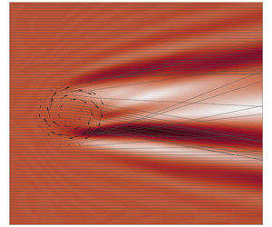
Wave rays due to  $\boldsymbol{k}_{0}$ over a jet-like current field indicated by the solid lines. The rays at $x_{1}=0$ are obliquely incident with an angle of $15^{\circ }$. In addition, the ambient current is marked by arrows. Finally, the dashed vertical lines are sections along which the results of the significant wave height will be displayed.

2.5 Set-up and overview of the considered numerical simulations
Two classical examples of wave–current interactions are considered. The first concerns the evolution of an incoming wave field over a jet-like current. This example is used to verify the model in § 3. In the second example, the field interacts with a vortex-ring current. This example is used in § 4 to study the statistical condition for the effect of wave interferences to appear. A visual description of the spatial variation of the considered current fields is presented by the arrows in figure 1 for the jet-like current and in figure 4 for the vortex ring. Mathematically, these current fields are defined as follows. The jet is defined as
 $$\begin{eqnarray}\left.\begin{array}{@{}c@{}}\boldsymbol{U}(x_{1},x_{2})=[U_{x_{1}},0],\\ U_{x_{1}}=C_{1}f[\tanh [(x_{2}+R)/(C_{2}R)]-\tanh [(x_{2}-R)/(C_{2}R)]],\\ f=1+\tanh [(x_{1}-R)/(C_{2}R)],\end{array}\right\}\end{eqnarray}$$
 where  $R=200~\text{m}$, $C_{1}=-0.1~\text{m}~\text{s}^{-1}$ and $C_{2}=0.5$. In this case, the maximum opposing current value is $|U_{x_{1}}\!|_{max}=0.38~\text{m}~\text{s}^{-1}$. Using cylindrical coordinates, the definition of the vortex ring is given by (Mapp et al. Reference Mapp, Welch and Munday1985)
 $$\begin{eqnarray}\left.\begin{array}{@{}c@{}}\boldsymbol{U}(r,\unicode[STIX]{x1D703})=[0,U_{\unicode[STIX]{x1D703}}],\\ U_{\unicode[STIX]{x1D703}}=\left\{\begin{array}{@{}l@{}}C_{1}(r/R_{1})^{2},~~r\leqslant R_{1},\\ C_{2}\exp [-(R_{2}-r)^{2}/R_{3}^{2}],\,r\geqslant R_{1},\\ \end{array}\right.\end{array}\!\!\right\}\end{eqnarray}$$
 for which the values of  $R_{1}$, $R_{2}$, $R_{3}$, $C_{1}$ and $C_{2}$ were chosen identical to those detailed in Belibassakis et al. (Reference Belibassakis, Gerostathis and Athanassoulis2011). In this case, the maximum current value is $|U_{\unicode[STIX]{x1D703}}|_{max}=1.00~\text{m}~\text{s}^{-1}$.
Both of these examples are formulated over a spatial domain of  $4000~\text{m}\times 4000~\text{m}$ and a constant depth of $h=10~\text{m}$. Waves enter the domain along the left-hand boundary, on $x_{1}=0$. This is simulated by prescribing an incoming energy density, $E_{0}=E(x_{1}=0,x_{2},k_{1},k_{2})$. Note that, as the incoming wave field is assumed to be statistically homogeneous, the corresponding boundary condition of the Wigner distribution is readily obtained as follows: $W_{0}=E_{0}/\unicode[STIX]{x1D70E}$. Finally, note that the lateral boundaries are treated as periodic.
An overview of the considered simulations in terms of their physical, statistical and numerical parameters.

An overview of the simulations considered in this study is given in table 1. These simulations differ by the current type (indicated by the name of the simulation in the first column of the table) and by the parameters characterizing the incoming spectrum,  $E_{0}$. In all the simulations the incoming spectrum, $E_{0}$, is defined as a two-dimensional Gaussian centred around $\boldsymbol{k}_{0}$. The incoming spectrum is therefore defined completely by the significant wave height ${H_{s}}_{0}$, the carrier wave period and direction $T_{0}$ and $\unicode[STIX]{x1D703}_{0}$ (which provide the centre point $\boldsymbol{k}_{0}$ through the linear dispersion relation) and the standard deviation $S_{d}^{(k)}$, which are given in the second, third, fourth and fifth column of table 1, respectively. In order to give a more intuitive physical interpretation of the width of the spectrum, the table also provides the corresponding standard deviations of the transformed spectrum written in terms of frequency and direction, $S_{d}^{(f)}$ and $S_{d}^{(\unicode[STIX]{x1D703})}$, given in the sixth and seventh columns. Numerically, $E_{0}$ is represented over the grid $N_{k}$ with a resolution that is determined by $S_{d}^{(k)}$ and the resolution parameter $\unicode[STIX]{x1D6FC}$ (see appendix E) given in the eighth column. The value of $\unicode[STIX]{x0394}x$, on the other hand, cannot be deduced from the table; appendix E guides how to choose a reasonable value for $\unicode[STIX]{x0394}x$. This value is fixed to $\unicode[STIX]{x0394}x=25$ m for all the simulations. In addition, the table also provides the correlation length, $L_{c}$, and the statistical parameter, $\unicode[STIX]{x1D6FD}$, in the ninth and tenth columns. As outlined in appendix E, $L_{c}$ is evaluated using $S_{d}^{(k)}$. This can also be expected by the scaling property of the Fourier transform ( $O(L_{c})=O(2/S_{d}^{(k)})$). Throughout the analysis of the results in the following subsections, the value of $L_{c}$ (as opposed to the value taken into account in the numerical model; see appendix E) is defined as $L_{c}=4/S_{d}^{(k)}$. For the considered Gaussian initial distribution, this value equals the so-called $1/\text{e}^{2}$ width that provides the diameter connecting the two points with $1/\text{e}^{2}$ times the maximum value of the correlation function. Finally, the order of magnitude of $\unicode[STIX]{x1D6FD}$ is obtained following its definition, $\unicode[STIX]{x1D6FD}=L_{c}/L_{m}$.
3 Model verification
The main aim of this section is to verify the performance of the QCM. The model is verified through a comparison with REF/DIF 1 (Kirby and Dalrymple Reference Kirby and Dalrymple1986), which solves a parabolic approximation of the well-known mild-slope equation (e.g. Dingemans Reference Dingemans1997). Since REF/DIF 1 allows for monochromatic, unidirectional forcing at the incident boundary, statistics for multi-directional and irregular incident waves are constructed by superposition of variances, under the assumption that waves at the incident boundary are statistically independent (see details in Chawla et al. (Reference Chawla, Özkan-Haller and Kirby1998)). Additionally, to demonstrate the statistical contribution of the interference terms, the results of the QCM are also compared to the results of the SWAN model (Booij et al. Reference Booij, Ris and Holthuijsen1999). To this end, the first two simulations detailed in table 1, namely  $\text{Jet}_{1}$ and $\text{Jet}_{2}$, are considered.
The simulations  $\text{Jet}_{1}$ and $\text{Jet}_{2}$ describe the evolution of waves over the jet-like current field. Ray tracing results (figure 1) show that for this jet-like current the waves refract and form a focal zone close to $x_{1}=2000~\text{m}$, beyond which interference structures may emerge.
The physical pattern described by the rays in figure 1 is also reflected statistically in the results of figures 2 and 3. While the results of the QCM and of REF/DIF 1 agree well and share a similar evolution pattern before and after the crossing zone in both of the simulations, the SWAN results increasingly deviate beyond the crossing zone, where interference effects emerge (see figures 2a–c and 3a,b) (note that the small differences that arise at the lateral boundaries, as for instance that appear in the results of figure 3(b) are due to different boundary conditions assumed in each of the models). The results also show that interference effects are not confined to caustic regions (where geometric optics break down), but rather spread over much greater distances in the down-wave direction, beyond the crossing zone (e.g. figure 2a–c). The differences between the models are less pronounced in the results of simulation  $\text{Jet}_{2}$ which is initiated using a broader spectrum (see figures 2d–f and 3c,d). In this case, all three models qualitatively predict a similar spatial structure of $H_{s}$ throughout the domain.
Comparison between QCM, REF/DIF 1 and SWAN in terms of the spatial distribution of the significant wave height. (a–c) The results of the simulation  $\text{Jet}_{1}$;(d–f) the results due to $\text{Jet}_{2}$.

Comparison between QCM, REF/DIF 1 and SWAN in terms of the significant wave height along the sections that are indicated in figure 1. (a,b) The results of the simulation  $\text{Jet}_{1}$; (c,d) the results due to $\text{Jet}_{2}$.

Model differences are principally due to the statistical contribution of wave interferences. The transport equation employed by third-generation spectral models (e.g. SWAN), equation (2.18), disregards the contribution of cross-correlations (correlations of different wave components), which contain the information about wave interference. The QCM, on the other hand, does account for this information, and therefore, as the statistical contribution of wave interference becomes significant, the discrepancies between the results of the QCM (or REF/DIF 1) and SWAN are more pronounced. Therefore, it is necessary to understand under which conditions the effect of wave interferences is important.
Generally speaking, the importance of the interference effects reduces as the spectrum of the incoming field becomes wider (e.g. Vincent & Briggs Reference Vincent and Briggs1989). Effectively, the multiple out-of-phase interference patterns generated by each wave component of the incoming field cancel each other out. Consequently, the superposition of the interference patterns becomes smoother as the incoming spectrum becomes wider. This is the reason why differences between the QCM (and REF/DIF 1) and SWAN are larger for  $\text{Jet}_{1}$ than $\text{Jet}_{2}$. Whether or not interference effects can be expected may formally be related to the ratio $\unicode[STIX]{x1D6FD}$ between the correlation length scale of the incident wave field, $L_{c}$, and a typical length scale of the medium, $L_{m}$. Interference effects may become significant when $\unicode[STIX]{x1D6FD}\geqslant O(1)$ and are more pronounced for larger values of $\unicode[STIX]{x1D6FD}$ (hence the difference between $\text{Jet}_{1}$ and $\text{Jet}_{2}$). This statistical condition is discussed in detail next.
4 Discussion
The statistical contribution of wave interferences as a function of the parameter  $\unicode[STIX]{x1D6FD}$ can be analysed conceptually as follows. Consider a certain point in space beyond the crossing zone, where interference effects are expected to play a role and assuming that the incoming field is monochromatic, for which $\unicode[STIX]{x1D6FD}\rightarrow \infty$. In this case, the correlation function at the considered point will extend over a very large spatial domain ( $L_{c}\rightarrow \infty$), and will generally be composed of in-phase variance terms of the scattered field and out-of-phase cross-correlation terms between each pair of scattered waves. The cross-correlation terms include contributions that were generated due to correlation between the incoming field and the interference structures it forms. As the spectrum of the incoming field becomes wider (namely $S_{d}^{(k)}$ becomes larger), the correlation function will extend over smaller domains and, accordingly, $\unicode[STIX]{x1D6FD}$ will take smaller values. The corresponding change in the interference effect can be analysed from the physical point of view, by examining the correlation function, $\unicode[STIX]{x1D6E4}$, or from the spectral point of view, by considering the Wigner distribution, $W$. From the physical point of view, when the incoming spectrum becomes wider and $\unicode[STIX]{x1D6FD}$ reduces, the correlation value between the incoming field and the interference pattern it forms will become smaller, and consequently the contribution of wave interference, at the considered point, reduces as well. In the limit when $\unicode[STIX]{x1D6FD}\rightarrow 0$ (and therefore $L_{c}\rightarrow 0$), this correlation value converges to zero and the contribution of wave interference is eliminated.
Wave rays due to  $\boldsymbol{k}_{0}$ over a vortex ring. The rays are indicated by the solid lines, and the ambient current is marked by arrows. Note that in this case, the rays at $x_{1}=0$ are normally incident. Additionally, the dashed vertical lines are sections along which the results of the significant wave height will be displayed. Finally, the dotted lines distinguish between different regions of the wave field.

The spectral point of view examines the representation of the cross-correlation terms in the Wigner distribution. Since the phases of the cross-correlation terms are not necessarily zero, their amplitudes may either be positive or negative, and therefore tend to cancel each other and lose intensity. As a result, when the Wigner distribution at the considered point is integrated over the spectral space for the purpose of computing the total variance, and the corresponding value of, say  $H_{s}$, the contribution of the cross-correlation terms will be less pronounced with the increasing of $S_{d}^{(k)}$, and therefore less pronounced with the decreasing of $\unicode[STIX]{x1D6FD}$.
The distribution of the significant wave height due to the interaction between waves and a vortex ring. The panels (a,b) present the results of  $\text{Ring}_{1}$ and the panels (c,d) present the results due to $\text{Ring}_{3}$. Additionally, the solid lines represent the wave rays due to $\boldsymbol{k}_{0}$. Finally, the three black points denoted by $P_{1}$, $P_{2}$ and $P_{3}$ indicate the spatial path along which the evolution of the correlation function and the Wigner distribution is considered. Point $P_{1}$ is located at $(1000~\text{m},-525~\text{m})$, $P_{2}$ at $(2000~\text{m},-625~\text{m})$ and $P_{3}$ at $(3000~\text{m},-725~\text{m})$.

4.1 The evolution of the cross-correlation terms
This subsection provides a numerical demonstration of the above discussion of the statistical condition to the appearance of interference effects in the scattered field. The interaction problem between waves and a vortex ring is a convenient example for this purpose. This is due to the fact that in this case, the domain essentially consists of two homogeneous regions separated by a scattering region, which are referred to as the ‘incoming field’, the ‘scatterer’ and the ‘scattered field’, respectively (see figure 4). Consequently, the statistical condition to wave interferences, which says that correlation should emerge between the incoming field and the interference structure it forms, is readily demonstrated through this interaction problem, as it can be replaced by the condition that the correlation function should extend over a larger domain than the effective domain of the vortex ring.
The statistical condition to the appearance of interference effects is examined by considering the evolution of the correlation function and the Wigner distribution for simulations  $\text{Ring}_{1}$ and $\text{Ring}_{3}$ (which differ in their initial spectrum width; see table 1) over a specific spatial path. The spatial path was selected such that it would pass over an area where $H_{s}$ is significantly affected by wave interferences (see figure 5). Finally, the contribution of the interference terms is emphasized by comparing the results of the QCM to the corresponding results of SWAN.
In order to identify wave interference effects, the manner in which the cross-correlation terms (which represent the contribution of wave interferences) are represented is explained first (refer also to the definitions in (2.8) and (2.9)). Given two correlated wave components, their contribution in the correlation function results in two variance terms with wavenumbers  $\boldsymbol{k}_{1}$ and $\boldsymbol{k}_{2}$, and cross-correlation term (or interference term) with a wavenumber $(\boldsymbol{k}_{1}+\boldsymbol{k}_{2})/2$. The amplitude of the cross-correlation term depends on the amplitudes of the two wave components and their phase difference. If the point around which the correlation function is considered is located at the trough of the interference pattern generated by the two waves, then the amplitude of the cross-correlation term will be negative and vice versa. Also recall that the correlation function presented here follows the definition in (2.7). Consequently, $\unicode[STIX]{x1D6E4}(\boldsymbol{x},\boldsymbol{x}^{\prime })$ is the correlation between $\unicode[STIX]{x1D713}(\boldsymbol{x}+\boldsymbol{x}^{\prime }/2)$ and $\unicode[STIX]{x1D713}^{\ast }(\boldsymbol{x}-\boldsymbol{x}^{\prime }/2)$, which is different from the function that defines the correlation between $\unicode[STIX]{x1D713}(\boldsymbol{x})$ and $\unicode[STIX]{x1D713}^{\ast }(\boldsymbol{x}+\boldsymbol{x}^{\prime })$.
The evolution of the correlation function (a–c) and the corresponding Wigner distribution (d–f) as presented by the spatial points  $P_{1}$, $P_{2}$ and $P_{3}$. The values of the results are normalized by $|\unicode[STIX]{x1D6E4}(P_{j},\boldsymbol{x}^{\prime })|_{max}$ and $|W(P_{j},\boldsymbol{k})|_{max}$. These results were obtained for the simulation $\text{Ring}_{1}$ using the QCM.

The analysis starts by examining the evolution results of the correlation function and the Wigner distribution for the simulation  $\text{Ring}_{1}$. In this case $\unicode[STIX]{x1D6FD}>1$, and therefore the effect of the cross-correlation terms on the structure of the correlation function and the Wigner distribution is likely to be significant. This is indeed evident by comparing the results of the QCM (figure 6) to the results of SWAN (figure 7). Notable differences clearly appear in the results around $P_{2}$ and $P_{3}$, in the ‘scattered field’, where interference effects are significant. Both of these points are located along the trough of the interference pattern (see figure 5). Indeed, the amplitudes of the cross-correlation terms, which are obtained at these points, are negative, as indicated by the blue areas in the Wigner distribution due to the QCM. Note that these blue areas are located exactly between the red areas which relate to the amplitudes of the variance terms. As expected, the blue areas do not appear in the action density spectrum due to SWAN, as it disregards the cross-correlation terms and only accounts for the variance terms. Moreover, in contrast to SWAN’s results which only accounts for variance terms that are crossing close to the considered points, the QCM also includes contribution of variance terms and related cross-correlation terms that are crossing at some distance away from the considered points. This can be seen by comparing the Wigner distribution due to the QCM and the action density spectrum due to SWAN and by referring to the wave rays in figure 4. Finally, note that the variance areas in the Wigner distribution are somewhat more spread than the corresponding variance areas appearing in the action density spectrum.
The negative values of the cross-correlation amplitudes in the results due to the QCM lead to the fact that the correlation function at these points does not provide the maximum correlation value at its centre (i.e. at  $\boldsymbol{x}^{\prime }=0$). Conversely, since the SWAN model ignores the cross-correlation terms, the correlation function will always obtain the maximum value at $\boldsymbol{x}^{\prime }=0$. Therefore, the correlation function as defined in (2.7) does not necessarily show the maximum value at $\boldsymbol{x}^{\prime }=0$ for inhomogeneous fields.
Besides changing the correlation value at the central point, it is difficult to identify the cross-correlation terms directly through the correlation function. However, it is clear that these terms significantly change the structure of the correlation function, as reflected by the differences in the results due to the QCM and SWAN (compare figures 6a–c and 7a–c).
The evolution of the correlation function (a–c) and the corresponding action density spectrum (d–f) as presented by the spatial points  $P_{1}$, $P_{2}$ and $P_{3}$. The values of the results are normalized by $|\unicode[STIX]{x1D6E4}(P_{j},\boldsymbol{x}^{\prime })|_{max}$ and $|N(P_{j},\boldsymbol{k})|_{max}$. These results were obtained for the simulation $\text{Ring}_{1}$ using SWAN.

The significant contribution of wave interferences appearing in the results around  $P_{2}$ and $P_{3}$ implies that correlation emerges between the ‘incoming field’ and the ‘scattered field’. This is indeed shown by the results of the correlation function around $P_{1}$ in figure 6 (or in figure 7). The results show that the correlation function extends over a much larger domain than the effective domain of the vortex ring and that strong correlation values emerge between the incoming and the scattered field. Accordingly, the generated cross-correlation terms at $P_{1}$ have a clear signature on the structure of the correlation function and the Wigner distribution due to the QCM (compare the results of $P_{1}$ in figures 6 and 7). These cross-correlation terms are transported along with the variance terms, altering dramatically the statistics of the scattered field, as shown by the significant differences between the results of the QCM and SWAN around $P_{2}$ and $P_{3}$.
The evolution of the correlation function (a–c) and the corresponding Wigner distribution (d–f) as presented by the spatial points  $P_{1}$, $P_{2}$ and $P_{3}$. The values of the results are normalized by $|\unicode[STIX]{x1D6E4}(P_{j},\boldsymbol{x}^{\prime })|_{max}$ and $|W(P_{j},\boldsymbol{k})|_{max}$. These results were obtained for the simulation $\text{Ring}_{3}$ using the QCM. Note that the scale over which the correlation function is plotted is much smaller than the corresponding scale used to present the results for $\text{Ring}_{1}$.

The differences in the results between the QCM and SWAN for the simulation  $\text{Ring}_{3}$ are much less prominent (see figures 8 and 9). The reason for this is that at $P_{1}$, the correlation function extends over a domain with about the same diameter as that of the vortex ring, and only small correlation value arises between the incoming field and the interference structure it forms in the vicinity of the crossing point at $(x_{1},x_{2})=(1365~\text{m},-355~\text{m})$ (see figure 5). As a consequence, at $P_{1}$, the amplitudes of the generated cross-correlation terms are quite low, as shown by the blue area in the Wigner distribution due to the QCM in figure 8. Over the ‘scattered field’ region, at $P_{2}$ and $P_{3}$, the influence of the cross-correlation terms is hardly detected through the correlation function, and, indeed, at these points the correlation functions due to the QCM and SWAN are almost identical. However, the presence of the cross-correlation terms is visible in the Wigner distribution due to the QCM by the blue area located between the variance areas. These cross-correlation terms eventually result in a limited contribution to the statistics of the scattered field, as for instance appears by the spatial distribution of $H_{s}$ in figure 5.
The evolution of the correlation function (a–c) and the corresponding action density spectrum (d–f) as presented by the spatial points  $P_{1}$, $P_{2}$ and $P_{3}$. The values of the results are normalized by $|\unicode[STIX]{x1D6E4}(P_{j},\boldsymbol{x}^{\prime })|_{max}$ and $|N(P_{j},\boldsymbol{k})|_{max}$. These results were obtained for the simulation $\text{Ring}_{3}$ using SWAN. Note that the scale over which the correlation function is plotted is much smaller than the corresponding scale used to present the results for $\text{Ring}_{1}$.

To conclude, the examination of the evolution of the correlation function and the Wigner distribution verifies the statistical condition for the generation of cross-correlation as was introduced conceptually in the beginning of this section. Moreover, the examination also demonstrates numerically that the correlation value between the incoming field and the interference structure it forms determines the dominance of the interference patterns in the scattered field.
4.2 The validity of the QCM
The final issue that is discussed here is the validity of the QCM versus the validity of SWAN over the parameter  $\unicode[STIX]{x1D6FD}$. As was explained in the derivation of the QCM in § 2.3 and following the presentation of the results so far, the QCM, in contrast to SWAN, seems to remain statistically valid for $\unicode[STIX]{x1D6FD}\geqslant O(1)$. The reason for this was extensively discussed in the previous subsection, and in short is simply because the QCM accounts for statistical inhomogeneity of the wave field, generated due to interference effects.
On the validity of the QCM (a,b) and SWAN (c,d) over the parameter  $\unicode[STIX]{x1D6FD}$, shown through the convergence of the significant wave height to the result of REF/DIF 1 with $\text{Ring}_{1}$. The results are given along Sections A and B that are indicated in figure 4.

On the validity of the QCM (a,b) and SWAN (c,d) over the parameter  $\unicode[STIX]{x1D6FD}$, shown through the convergence of the significant wave height to the result of REF/DIF 1 with $\text{Ring}_{1}$. The results are given along Sections C and D that are indicated in figure 4.

The validity of the QCM over  $\unicode[STIX]{x1D6FD}$ is presented by demonstrating the convergence of its results, obtained with an increasing value of $\unicode[STIX]{x1D6FD}$, to a single result of REF/DIF 1 obtained with a specific high value of $\unicode[STIX]{x1D6FD}$. To this end, the QCM is used to compute $H_{s}$ along the sections shown in figure 4 using simulations $\text{Ring}_{1}$, $\text{Ring}_{2}$ and $\text{Ring}_{3}$ which are defined with a decreasing value of $\unicode[STIX]{x1D6FD}$ (i.e. $\text{Ring}_{1}$ is defined with the highest $\unicode[STIX]{x1D6FD}$ value, whereas $\text{Ring}_{3}$ is defined with the lowest $\unicode[STIX]{x1D6FD}$ value; see also table 1). In addition, the result due to REF/DIF 1 is obtained through $\text{Ring}_{1}$. Finally, the convergence of the QCM results to the result of REF/DIF 1 is shown in figures 10(a,b) and 11(a,b). The same procedure is performed using SWAN and is presented in figures 10(c,d) and11(c,d).
Over the ‘scatterer’ region, before the focusing zones, SWAN seems to remain valid (see figure 10, section A) even for the highest  $\unicode[STIX]{x1D6FD}$ considered, which corresponds to the simulation $\text{Ring}_{1}$. However, over the ‘scattered field’ region, where interference effects emerge, SWAN does not converge to REF/DIF 1 when $\unicode[STIX]{x1D6FD}$ increases. On the other hand, the QCM does converge to REF/DIF 1, and seems to remain valid for the scattered field as well.
It is important to remember that the capabilities of the QCM over  $\unicode[STIX]{x1D6FD}$ involve a constraint. This constraint is that $\unicode[STIX]{x1D716}\ll 1$, introduced by the deterministic model, equation (2.6), which underlies the development of the QCM. Finally, recall that the QCM is also limited to small values of $\unicode[STIX]{x1D707}$, which basically limits its capabilities to accurately evolve interference terms with a wavelength of $L_{W}\leqslant O(L)$, where $L$ is the wavelength of the considered point $\boldsymbol{k}$ (see details in Smit & Janssen (Reference Smit and Janssen2013)).
5 Conclusions
This study presents the development of a statistical model for problems of wave–current interaction, taking into account the effect of wave interferences. The theoretical basis of this model lies in the definition of the Wigner distribution,  $W$, and of the action variable, $\unicode[STIX]{x1D713}$. This distribution provides a complete spectral description of the second-order statistics of the wave field. It includes cross-correlation terms, which provide the statistical information about wave interferences. As such, $W$ generalizes the concept of the action density spectrum, $N$, which only accounts for the information of wave variances.
Using the procedure described in Smit & Janssen (Reference Smit and Janssen2013) and Smit et al. (Reference Smit, Janssen and Herbers2015a), an evolution model for  $W$ (the QCM) is developed. This model provides a generalization of the conventional action balance model (presently employed by third-generation spectral wave models, e.g. SWAN and WAVEWATCH III), by allowing the generation and transportation of statistical wave interferences.
The effect of wave interferences can contribute significantly for cases where the variation scale of the medium is of the same order or smaller than the scale of the correlation length, namely for cases in which  $\unicode[STIX]{x1D6FD}\geqslant O(1)$. This statistical condition is explicitly examined for scenarios where the incoming field is statistically homogeneous, but develops inhomogeneity while propagating over ambient currents. Specifically, in order to obtain a statistical signature of wave interferences, the incident and scattered fields should be correlated, with the dominance of the interference effect determined by the correlation value itself.
In cases where this correlation is strong, the interference patterns alter the statistics of the field significantly. The resulting effect on the significant wave height,  $H_{s}$, is demonstrated through two examples of wave–current interaction and by a comparison to the SWAN model. It is demonstrated that in such cases, interference effects dramatically change the distribution of $H_{s}$, not only in the vicinity of wave-focusing areas, but also at a significant distance away from the focusing points.
It is therefore concluded that for regions involving rapid variability in medium (e.g. coastal regions or oceanic regions which tend to contain submesoscale currents), consideration of the statistical information of wave interference might by crucial for many applications, such as wave-induced circulation and transport processes in coastal regions or for prediction of extreme elevations in the open ocean.
Acknowledgements
This work is part of the research programme Earth and Life Sciences (ALW) with project number ALWOP.167, which is (partly) financed by the Dutch Research Council (NWO). P.S. acknowledges support by the Office of Naval Research (N00014-16-1-2856).
Declaration of interests
The authors report no conflict of interest.
Appendix A. The Weyl operator and its asymptotic form
The purpose of this appendix is to provide the definition of the pseudo-differential operators employed in this study. To this end, the operator  $\unicode[STIX]{x1D714}(\boldsymbol{x},-\text{i}\unicode[STIX]{x1D735}_{\boldsymbol{x}})$ will serve as a representative (the following also applies to the operators $\unicode[STIX]{x1D70E}(\boldsymbol{x},-\text{i}\unicode[STIX]{x1D735}_{\boldsymbol{x}})$ and $a(\boldsymbol{x},-\text{i}\unicode[STIX]{x1D735}_{\boldsymbol{x}})$ that were introduced in § 2). Additionally, for convenience, the expressions in this appendix (and in appendix B) are presented using the slow scale coordinates $\boldsymbol{x}_{m}=\unicode[STIX]{x1D716}\boldsymbol{x}$ and $t_{m}=\unicode[STIX]{x1D716}t$. However, in order to avoid cumbersome formulations, the subscript $m$ indicating these slow scale coordinates will be removed, keeping in mind that for the purposes of this appendix (and appendix B), $\boldsymbol{x}$ and $t$ are now serving as the slow scale coordinates. An additional notation is $D_{j}$, which will be used here and in the following appendices to represent the operator $-\text{i}\unicode[STIX]{x1D735}_{j}$.
The definition of the pseudo-differential  $\unicode[STIX]{x1D714}(\boldsymbol{x},\unicode[STIX]{x1D716}D_{\boldsymbol{x}})$ is based on its association with a ‘phase-space’ symbol (a function which is defined in $(\boldsymbol{x},\boldsymbol{k})$ space). Here, it is assumed that such a ‘phase-space’ symbol can be defined locally (in this case, it is the usual dispersion relation, equation (2.1)), which basically requires that the characteristic length scale of the medium variation is much larger than the considered wavelength (e.g. Dingemans Reference Dingemans1997), i.e. that $\unicode[STIX]{x1D716}\ll 1$.
Given a ‘phase-space’ symbol, the corresponding operator in the physical space can be defined through the association between  $\boldsymbol{k}$ and $D_{\boldsymbol{x}}$. However, because $\boldsymbol{x}$ and $D_{\boldsymbol{x}}$ do not commute, one must follow an association rule for an arbitrary symbol. Here, the Weyl rule of association is adopted (e.g. Cohen Reference Cohen2012), which is defined through the following Fourier transform of $\unicode[STIX]{x1D714}(\boldsymbol{x},\boldsymbol{k})$:
 $$\begin{eqnarray}\unicode[STIX]{x1D714}(\boldsymbol{x},\boldsymbol{k})=\int \hat{\unicode[STIX]{x1D714}}(\boldsymbol{q},\boldsymbol{p})\exp (\text{i}\boldsymbol{q}\boldsymbol{\cdot }\boldsymbol{x}+\text{i}\boldsymbol{p}\boldsymbol{\cdot }\boldsymbol{k})\,\text{d}\boldsymbol{q}\,\text{d}\boldsymbol{p}.\end{eqnarray}$$
 Then, the Weyl operator is obtained by substituting the operator  $\unicode[STIX]{x1D716}D_{\boldsymbol{x}}$ instead of $\boldsymbol{k}$, which provides the following expression:
 $$\begin{eqnarray}\unicode[STIX]{x1D714}(\boldsymbol{x},\unicode[STIX]{x1D716}D_{\boldsymbol{x}})=\int \hat{\unicode[STIX]{x1D714}}(\boldsymbol{q},\boldsymbol{p})\exp (\text{i}\boldsymbol{q}\boldsymbol{\cdot }\boldsymbol{x}+\text{i}\unicode[STIX]{x1D716}\boldsymbol{p}\boldsymbol{\cdot }D_{\boldsymbol{x}})\,\text{d}\boldsymbol{q}\,\text{d}\boldsymbol{p}\end{eqnarray}$$
 and which can be simplified using the commutator value,  $[\text{i}\boldsymbol{q}\boldsymbol{\cdot }\boldsymbol{x},\unicode[STIX]{x1D716}i\boldsymbol{p}\boldsymbol{\cdot }D_{\boldsymbol{x}}]=-\text{i}\unicode[STIX]{x1D716}\boldsymbol{q}\boldsymbol{\cdot }\boldsymbol{p}$, to obtain
 $$\begin{eqnarray}\unicode[STIX]{x1D714}(\boldsymbol{x},\unicode[STIX]{x1D716}D_{\boldsymbol{x}})=\int \hat{\unicode[STIX]{x1D714}}(\boldsymbol{q},\boldsymbol{p})\exp \left({\displaystyle \frac{\text{i}}{2}}\unicode[STIX]{x1D716}\boldsymbol{q}\boldsymbol{\cdot }\boldsymbol{p}\right)\exp (\text{i}\boldsymbol{q}\boldsymbol{\cdot }\boldsymbol{x})\exp (\text{i}\unicode[STIX]{x1D716}\boldsymbol{p}\boldsymbol{\cdot }D_{\boldsymbol{x}})\,\text{d}\boldsymbol{q}\,\text{d}\boldsymbol{p}.\end{eqnarray}$$
 An important step is to define the asymptotic form of the Weyl operator, which will be used quite often to understand and interpret the leading-order results of its operation on a certain variable. As shown below, this asymptotic form depends on a Taylor expansion of the dispersion relation, and therefore (at least conceptually) should be defined around  $\boldsymbol{k}_{0}\neq 0$, since derivatives of the dispersion relation at $\boldsymbol{k}=0$ are singular. In order to obtain the asymptotic form of the Weyl operator, the Fourier transform of the dispersion relation around $\boldsymbol{k}_{0}$ is replaced by the Taylor expansion of the dispersion relation around that point:
 $$\begin{eqnarray}\displaystyle \unicode[STIX]{x1D714}(\boldsymbol{x},\unicode[STIX]{x1D716}D_{\boldsymbol{x}}) & = & \displaystyle \int [\exp (\text{i}\overline{\boldsymbol{k}}\boldsymbol{\cdot }D_{\boldsymbol{k}})\hat{\unicode[STIX]{x1D714}}(\boldsymbol{q},\boldsymbol{k})]_{\boldsymbol{k}=\boldsymbol{k}_{0}}\exp (-\text{i}\boldsymbol{p}\boldsymbol{\cdot }\overline{\boldsymbol{k}})\exp \left({\displaystyle \frac{\text{i}}{2}}\unicode[STIX]{x1D716}\boldsymbol{q}\boldsymbol{\cdot }\boldsymbol{p}\right)\nonumber\\ \displaystyle & & \displaystyle \times \,\exp (\text{i}\boldsymbol{q}\boldsymbol{\cdot }\boldsymbol{x})\exp (\text{i}\boldsymbol{p}\boldsymbol{\cdot }(\unicode[STIX]{x1D716}D_{\boldsymbol{x}}-\boldsymbol{k}_{0}))\,\text{d}\overline{\boldsymbol{k}}\,\text{d}\boldsymbol{q}\,\text{d}\boldsymbol{p},\end{eqnarray}$$
 which, after Fourier transform with respect to  $\overline{\boldsymbol{k}}$, reduces to
 $$\begin{eqnarray}\displaystyle & & \displaystyle \hspace{-15.60004pt}\unicode[STIX]{x1D714}(\boldsymbol{x},\unicode[STIX]{x1D716}D_{\boldsymbol{x}})\nonumber\\ \displaystyle & & \displaystyle \hspace{-15.60004pt}\quad =\int \unicode[STIX]{x1D6FF}(\boldsymbol{p})\left[\exp (\text{i}\boldsymbol{q}\boldsymbol{\cdot }\boldsymbol{x})\exp \left[\text{i}\boldsymbol{p}\boldsymbol{\cdot }\left(\unicode[STIX]{x1D716}D_{\boldsymbol{x}}-\boldsymbol{k}_{0}+\unicode[STIX]{x1D716}{\displaystyle \frac{\boldsymbol{q}}{2}}\right)\right]\exp (\text{i}\overleftarrow{D}_{\boldsymbol{p}}\boldsymbol{\cdot }\overrightarrow{D}_{\boldsymbol{k}})\hat{\unicode[STIX]{x1D714}}(\boldsymbol{q},\boldsymbol{k})\right]_{\boldsymbol{k}=\boldsymbol{k}_{0}}\,\text{d}\boldsymbol{q}\,\text{d}\boldsymbol{p},\nonumber\\ \displaystyle & & \displaystyle\end{eqnarray}$$
and eventually leading to the following asymptotic form:
 $$\begin{eqnarray}\unicode[STIX]{x1D714}(\boldsymbol{x},\unicode[STIX]{x1D716}D_{\boldsymbol{x}})=\left[\unicode[STIX]{x1D714}(\boldsymbol{x},\boldsymbol{k})\exp \left({\displaystyle \frac{\text{i}}{2}}\unicode[STIX]{x1D716}\overleftarrow{D}_{\boldsymbol{x}}\boldsymbol{\cdot }\overleftarrow{D}_{\boldsymbol{k}}\right)\exp [\text{i}\overleftarrow{D}_{\boldsymbol{k}}\boldsymbol{\cdot }(\unicode[STIX]{x1D716}D_{\boldsymbol{x}}-\boldsymbol{k}_{0})]\right]_{\boldsymbol{k}=\boldsymbol{k}_{0}}.\end{eqnarray}$$
 In the following, the operation of the Weyl operator, using its asymptotic form, equation (A 6), is examined for two examples: the case of a plane wave over a homogeneous medium and the case of a plane wave propagating over a slowly varying medium. The operation of the Weyl operator in the first case is easily worked out, as in this case the dispersion relation is not a function of  $\boldsymbol{x}$, and also the spatial derivatives on the representative variable of the field can be resolved directly. This is demonstrated as follows. The plane wave is represented by the surface potential as $\unicode[STIX]{x1D719}=A\exp [\text{i}(\boldsymbol{k}_{0}\boldsymbol{\cdot }\boldsymbol{x}-\unicode[STIX]{x1D714}_{0}t)/\unicode[STIX]{x1D716}]$, and consequently the operation $\unicode[STIX]{x1D714}\unicode[STIX]{x1D719}$ is obtained by the following:
 $$\begin{eqnarray}\unicode[STIX]{x1D714}(\unicode[STIX]{x1D716}D_{\boldsymbol{x}})\unicode[STIX]{x1D719}=\unicode[STIX]{x1D714}(\boldsymbol{k}_{0})\unicode[STIX]{x1D719},\end{eqnarray}$$
which is the desired result as detailed at the beginning of appendix B.
In the second example, the considered wave component is represented by the surface potential as  $\unicode[STIX]{x1D719}=A(\boldsymbol{x})\exp [(S-\text{i}\unicode[STIX]{x1D714}_{0}t)/\unicode[STIX]{x1D716}]$. In this case, the operation of the Weyl operator is not immediately seen. The leading-order ( $O(1)$) term is obtained when the first exponent in (A 6) is taken to be equal to one, and the spatial derivative of the second exponent, $D_{\boldsymbol{x}}$, operates only on the exponent of $\unicode[STIX]{x1D719}$. This term is the dispersion relation, equation (2.1). Terms of $O(\unicode[STIX]{x1D716})$ are obtained for three different sets of conditions. Two of these sets instruct one to take the first exponent in (A 6) to be equal to one, and at each expansion order of the second exponent the spatial derivative, $D_{\boldsymbol{x}}$, should operate once on $A$ for the one set or once on $S$, as instructed by the other set. The third term is obtained using the second term of the expansion of the first exponent of the operator and when the spatial derivative of the second exponent, $D_{\boldsymbol{x}}$, operates only on the exponent of $\unicode[STIX]{x1D719}$. This description is summarized as follows:
 $$\begin{eqnarray}\displaystyle \unicode[STIX]{x1D714}(\boldsymbol{x},\unicode[STIX]{x1D716}D_{\boldsymbol{x}})\unicode[STIX]{x1D719} & = & \displaystyle \unicode[STIX]{x1D714}(\boldsymbol{x},D_{\boldsymbol{x}}S)\unicode[STIX]{x1D719}+\unicode[STIX]{x1D716}\text{i}\left(D_{\boldsymbol{x}}A\boldsymbol{\cdot }D_{\boldsymbol{k}}\unicode[STIX]{x1D714}+\frac{\text{i}}{2}AD_{\boldsymbol{x}}^{2}SD_{\boldsymbol{k}}^{2}\unicode[STIX]{x1D714}\right.\nonumber\\ \displaystyle & & \displaystyle \left.+\,\frac{1}{2}AD_{\boldsymbol{x}}\boldsymbol{\cdot }D_{\boldsymbol{k}}\unicode[STIX]{x1D714}\right)_{\boldsymbol{k}=D_{\boldsymbol{x}}S}\exp [(S-\text{i}\unicode[STIX]{x1D714}_{0}t)/\unicode[STIX]{x1D716}]+O(\unicode[STIX]{x1D716}^{2}).\end{eqnarray}$$
This closes the formal definition of the Weyl operator, equation (A 3), and its asymptotic form, equation (A 6). The operation of the Weyl operator on representative variables in the homogeneous and weakly inhomogeneous cases is used next to verify the evolution equation of the action variable,  $\unicode[STIX]{x1D713}$.
Appendix B. On the evolution equation of the action variable
This appendix aims to demonstrate that the starting point equation (the evolution equation of the action variable), equation (2.6), is exact for the case of linear wave propagation over a homogeneous medium, and reduces to the correct evolution equations for the weakly inhomogeneous case. In the latter, the correct evolution equations are the dispersion relation, equation (2.1), and the well-known action balance equation (e.g. Dingemans Reference Dingemans1997). For these purposes, the starting point equation, equation (2.6), is written once again, using the slow scale coordinates, as follows:
 $$\begin{eqnarray}\unicode[STIX]{x1D716}\unicode[STIX]{x2202}_{t}\unicode[STIX]{x1D713}=-\text{i}\unicode[STIX]{x1D714}(\boldsymbol{x},\unicode[STIX]{x1D716}D_{\boldsymbol{x}})\unicode[STIX]{x1D713},\end{eqnarray}$$
 where, as in the previous appendix, these slow scale coordinates are indicated using the same variable notation of the fast scale coordinates,  $\boldsymbol{x}$, $t$, in order to avoid cumbersome formulations.
As introduced, the first aim here is to show that the starting point equation, equation (B 1), describes exactly the correct solution of an incoming plane wave over a homogeneous medium. To this end, the following example will be worked out. Considering a specific domain of interest, the example assumes that into one of the domain’s boundaries enters a monochromatic wave field with an absolute frequency  $\unicode[STIX]{x1D714}_{0}$. In this case, the surface variables of the considered wave obey to the following form:
 $$\begin{eqnarray}\left.\begin{array}{@{}c@{}}\displaystyle \unicode[STIX]{x1D719}=A_{0}\exp [(S-\text{i}\unicode[STIX]{x1D714}_{0}t)/\unicode[STIX]{x1D716}]+\text{c.c.},\\ \displaystyle \unicode[STIX]{x1D702}=B_{0}\exp [(S-\text{i}\unicode[STIX]{x1D714}_{0}t)/\unicode[STIX]{x1D716}]+\text{c.c.},\end{array}\right\}\end{eqnarray}$$
 where  $B_{0}=\text{i}A_{0}(\unicode[STIX]{x1D714}_{0}-\boldsymbol{U}\boldsymbol{\cdot }(D_{\boldsymbol{x}}S))/g$, as follows from the linear relation between $\unicode[STIX]{x1D719}$ and $\unicode[STIX]{x1D702}$ (e.g. Dingemans Reference Dingemans1997):
 $$\begin{eqnarray}\unicode[STIX]{x1D702}=-\frac{1}{g}(\unicode[STIX]{x2202}_{t}+\boldsymbol{U}\boldsymbol{\cdot }\unicode[STIX]{x1D735}_{\boldsymbol{x}})\unicode[STIX]{x1D719}.\end{eqnarray}$$
 The wavenumber,  $D_{\boldsymbol{x}}S$, is constant, and the constant amplitude, $A_{0}$, assumed to be a ‘proper’ (e.g. Lapidoth Reference Lapidoth2017) Gaussian random variable, namely $\langle A_{0}^{2}\rangle =0$. The corresponding form of $\unicode[STIX]{x1D713}$ is obtained following its definition, equation (2.2):
 $$\begin{eqnarray}\unicode[STIX]{x1D713}=\frac{1}{\sqrt{2g}}[C_{0}\exp [(S-\text{i}\unicode[STIX]{x1D714}_{0}t)/\unicode[STIX]{x1D716}]+D_{0}\exp [(-S+i\unicode[STIX]{x1D714}_{0}t)/\unicode[STIX]{x1D716}]],\end{eqnarray}$$
 where the amplitudes  $C_{0}$ and $D_{0}$ are defined as $C_{0}=ga^{-1}B_{0}+\text{i}aA_{0}$ and $D_{0}=ga^{-1}B_{0}^{\ast }+\text{i}aA_{0}^{\ast }$, and, following (A 7), $a=\sqrt{\unicode[STIX]{x1D70E}(D_{x}S)}$. Using these starting points, it is now aimed to show that (B 1) produces the correct magnitude of $D_{\boldsymbol{x}}S$. By substituting (B 4) into (B 1), one obtains that the first solution (with the amplitude $C_{0}$) produces, as required, the equation $\unicode[STIX]{x1D714}_{0}=\unicode[STIX]{x1D714}(D_{\boldsymbol{x}}S)$. Substituting this result into the definition of $B_{0}$, which becomes $B_{0}=\text{i}A_{0}\unicode[STIX]{x1D70E}(D_{\boldsymbol{x}}S)/g$, provides the necessary result that $D_{0}=0$ (this is necessary, since the second term of $\unicode[STIX]{x1D713}$ is not a solution of (B 1)), whereas the value of $C_{0}$ is then given by $C_{0}=2\text{i}A_{0}\sqrt{\unicode[STIX]{x1D70E}(D_{\boldsymbol{x}}S)}$.
The second aim of this appendix is to show that the starting point equation (B 1) reduces to the correct evolution equations for the weakly inhomogeneous case. To do this, the same example as in the homogeneous case is considered. Following the Wentzel–Kramers–Brillouin method (e.g. Holmes Reference Holmes2012), and assuming that the bathymetry and the current are not time dependent, the surface velocity potential and elevation,  $\unicode[STIX]{x1D719}$ and $\unicode[STIX]{x1D702}$, can be defined to leading order in $\unicode[STIX]{x1D716}$ by (B 2), where now $A_{0}$ and $S$ are functions of $\boldsymbol{x}$. The corresponding leading-order definition of $\unicode[STIX]{x1D713}$ is given by (B 4), but now, following (A 8), $a=\sqrt{\unicode[STIX]{x1D70E}(\boldsymbol{x},D_{\boldsymbol{x}}S)}$. By substituting this definition into (B 1) and using the result of (A 8), the $O(1)$ eikonal equation is obtained to be $\unicode[STIX]{x1D714}_{0}=\unicode[STIX]{x1D714}(\boldsymbol{x},D_{\boldsymbol{x}}S)$, which can be written as
 $$\begin{eqnarray}\unicode[STIX]{x1D714}_{0}=\boldsymbol{U}\boldsymbol{\cdot }D_{\boldsymbol{x}}S+\unicode[STIX]{x1D70E}(\boldsymbol{x},D_{\boldsymbol{x}}S).\end{eqnarray}$$
 Using this result,  $B_{0}$ is obtained to be $B_{0}=\text{i}A_{0}\unicode[STIX]{x1D70E}(\boldsymbol{x},D_{\boldsymbol{x}}S)/g$, leading to the same necessary result as before, that $D_{0}=0$, whereas $C_{0}$ is given by $C_{0}=2\text{i}A_{0}\sqrt{\unicode[STIX]{x1D70E}(\boldsymbol{x},D_{\boldsymbol{x}}S)}$. The remaining unknown, $A_{0}$, is found through the following $O(\unicode[STIX]{x1D716})$ transport equation:
 $$\begin{eqnarray}\left(D_{\boldsymbol{x}}C_{0}\boldsymbol{\cdot }D_{\boldsymbol{k}}\unicode[STIX]{x1D714}+\frac{\text{i}}{2}C_{0}D_{\boldsymbol{x}}^{2}SD_{\boldsymbol{ k}}^{2}\unicode[STIX]{x1D714}+\frac{1}{2}C_{0}D_{\boldsymbol{x}}\boldsymbol{\cdot }D_{\boldsymbol{k}}\unicode[STIX]{x1D714}\right)_{\boldsymbol{k}=D_{\boldsymbol{x}}S}=0,\end{eqnarray}$$
which alternatively can be written as
 $$\begin{eqnarray}D_{\boldsymbol{x}}\boldsymbol{\cdot }(\langle |C_{0}|^{2}\rangle D_{\boldsymbol{ k}}\unicode[STIX]{x1D714})=0.\end{eqnarray}$$
 In order to verify that (B 7) is the well-known action balance equation (e.g. Dingemans Reference Dingemans1997), one should check that  $\unicode[STIX]{x1D70C}\langle |\unicode[STIX]{x1D713}|^{2}\rangle =\unicode[STIX]{x1D70C}\langle |C_{0}|^{2}\rangle$ indeed defines the mean action density. To see this, one may calculate $\langle |\unicode[STIX]{x1D713}|^{2}\rangle$ directly, using the definition of $\unicode[STIX]{x1D713}$, equation (2.2), which results in
 $$\begin{eqnarray}\unicode[STIX]{x1D70C}\langle |\unicode[STIX]{x1D713}|^{2}\rangle =\Big[{\displaystyle \frac{1}{2}}\unicode[STIX]{x1D70C}g\langle \unicode[STIX]{x1D702}_{0}^{2}\rangle +{\displaystyle \frac{1}{2g}}\unicode[STIX]{x1D70C}\langle (\unicode[STIX]{x1D70E}\unicode[STIX]{x1D719})_{0}^{2}\rangle \Big]/\unicode[STIX]{x1D70E}+O(\unicode[STIX]{x1D716}),\end{eqnarray}$$
 where the subscript  $0$ indicates $O(1)$ terms. The expression in the square brackets is exactly the mean energy density $m_{0}$ that was introduced in (2.5). Clearly, the first term of the expression represents the mean potential energy density, though the connection of the second term to the density of the kinetic energy might not be immediately obvious and should be clarified. Following (A 8), the first-order operation, $(\unicode[STIX]{x1D70E}\unicode[STIX]{x1D719})_{0}$, is defined as $(\unicode[STIX]{x1D70E}\unicode[STIX]{x1D719})_{0}=\unicode[STIX]{x1D70E}(\boldsymbol{x},D_{\boldsymbol{x}}S)\unicode[STIX]{x1D719}$. Substituting this result into (B 8), the second term becomes equal to the mean kinetic energy density for a homogeneous medium that is defined by the local values, $h(\boldsymbol{x})$ and $\boldsymbol{U}(\boldsymbol{x})$ (e.g. § 6.3 in Van Groesen and Molenaar (Reference Van Groesen and Molenaar2007)). Therefore, dividing the expression in the square brackets by the local intrinsic frequency, $\unicode[STIX]{x1D70E}$, leads to the definition of the mean action density (Bretherton & Garrett Reference Bretherton and Garrett1968).
Appendix C. From Wigner distribution to local energy
To motivate the necessity for an alternative formula that links the energy density,  $m_{0}$, and the Wigner distribution, $W(\boldsymbol{x},\boldsymbol{k},t)$, the following example is discussed (note that here the formulation returns to be written in terms of the original spatial coordinates, $\boldsymbol{x}$ and $t$). The example assumes an idealized sea state composed of three coherent and forward-propagating wave components in a one-dimensional and homogeneous medium. The waves are defined with the following wavenumbers: $k_{1}$, $k_{2}$ and $k_{3}=(k_{1}+k_{2})/2$. Accordingly, at a certain moment in time $t_{0}$, the wave field may be represented as follows:
 $$\begin{eqnarray}\left.\begin{array}{@{}c@{}}\displaystyle \unicode[STIX]{x1D719}=\mathop{\sum }_{n=1}^{3}A_{n}\exp (\text{i}k_{n}x)+\text{c.c.},\\ \displaystyle \unicode[STIX]{x1D702}=\mathop{\sum }_{n=1}^{3}B_{n}\exp (\text{i}k_{n}x)+\text{c.c.},\end{array}\right\}\end{eqnarray}$$
 where  $A_{n}$ and $B_{n}$ are complex random amplitudes. The amplitude $B_{n}$ is given by $B_{n}=\text{i}A_{n}\unicode[STIX]{x1D70E}_{n}/g$, as follows from the linear relation between $\unicode[STIX]{x1D719}$ and $\unicode[STIX]{x1D702}$ (see equation (B 3) in appendix B). The mean energy density, $m_{0}$ in this example, is derived using the expression in (2.5), and can be written as follows:
 $$\begin{eqnarray}m_{0}=\frac{2}{g}\mathop{\sum }_{n=1}^{3}\mathop{\sum }_{m=1}^{3}\unicode[STIX]{x1D70E}_{n}\unicode[STIX]{x1D70E}_{m}\langle A_{n}A_{m}^{\ast }\rangle \exp [\text{i}(k_{n}-k_{m})x].\end{eqnarray}$$
 The approach employed in this study to get to (C 2) is via the Wigner distribution of the action variable,  $\unicode[STIX]{x1D713}$, which for this example is given by
 $$\begin{eqnarray}W(x,k,t_{0})=\frac{2}{g}\mathop{\sum }_{n=1}^{3}\mathop{\sum }_{m=1}^{3}\sqrt{\unicode[STIX]{x1D70E}_{n}}\sqrt{\unicode[STIX]{x1D70E}_{m}}\langle A_{n}A_{m}^{\ast }\rangle \exp [\text{i}(k_{n}-k_{m})x]\unicode[STIX]{x1D6FF}\left[k-\frac{k_{n}+k_{m}}{2}\right],\end{eqnarray}$$
 where  $\unicode[STIX]{x1D6FF}(k)$ is now serving as the usual delta function. Now it can be seen explicitly that a simple substitution of (C 3) into (2.11) will not provide the result described in (C 2). As an example, consider the components in $W$ that multiply the function $\unicode[STIX]{x1D6FF}[k-(k_{1}+k_{2})/2]$. Following the definition of $k_{3}$, there are two such components, $2\unicode[STIX]{x1D70E}_{3}\langle |A_{3}|^{2}\rangle /g$ and $2\sqrt{\unicode[STIX]{x1D70E}_{1}}\sqrt{\unicode[STIX]{x1D70E}_{2}}\{\langle A_{1}A_{2}^{\ast }\rangle \exp [\text{i}(k_{1}-k_{2})x]+c.c\}/g$, which are related to the variance of the third wave component and to the correlation between the first and the second wave components, respectively. If $W$ is substituted into (2.11), both of these components will be factored by $\unicode[STIX]{x1D70E}_{3}$, which by referring to (C 2) will not lead to the correct interference term between the first and the second wave components. It is concluded that in order to calculate the mean energy density correctly, one must distinguish between the variance term and the interference terms for each $k$, and only then multiply by the correct factor. The derivation of an alternative formula to obtain $m_{0}$ based on $W$ is detailed below.
The starting point of the following derivation is the relation between the action varible,  $\unicode[STIX]{x1D713}$, and the mean energy density, $m_{0}$, as given in (2.4), recalling that $a(\boldsymbol{x},D_{\boldsymbol{x}})$ is a Weyl operator associated with the square root of the intrinsic angular frequency, $\unicode[STIX]{x1D70E}^{1/2}(\boldsymbol{x},\boldsymbol{k})$. Following the definition of the Weyl operator, the expression in (2.4) can be written as
 $$\begin{eqnarray}\displaystyle \hspace{-24.0pt}\langle |a(\boldsymbol{x},D_{\boldsymbol{x}})\unicode[STIX]{x1D713}|^{2}\rangle & = & \displaystyle \int \hat{a}(\boldsymbol{q}_{1},\boldsymbol{p}_{1})\hat{a}^{\ast }(\boldsymbol{q}_{2},\boldsymbol{p}_{2})\exp \left(\frac{\text{i}}{2}\boldsymbol{q}_{1}\boldsymbol{\cdot }\boldsymbol{p}_{1}+\frac{\text{i}}{2}\boldsymbol{q}_{2}\boldsymbol{\cdot }\boldsymbol{p}_{2}\right)\nonumber\\ \displaystyle \hspace{-24.0pt} & & \displaystyle \times \,\exp [\text{i}\boldsymbol{x}\boldsymbol{\cdot }(\boldsymbol{q}_{1}-\boldsymbol{q}_{2})]\langle \unicode[STIX]{x1D713}(\boldsymbol{x}+\boldsymbol{p}_{1},t)\unicode[STIX]{x1D713}^{\ast }(\boldsymbol{x}-\boldsymbol{p}_{2},t)\rangle \,\text{d}\boldsymbol{q}_{1}\,\text{d}\boldsymbol{q}_{2}\,\text{d}\boldsymbol{p}_{1}\,\text{d}\boldsymbol{p}_{2}.\end{eqnarray}$$
 By substituting the Fourier transform of the correlation function,  $\unicode[STIX]{x1D6E4}=\langle \unicode[STIX]{x1D713}(\boldsymbol{x}+\boldsymbol{p}_{1},t)\unicode[STIX]{x1D713}^{\ast }(\boldsymbol{x}-\boldsymbol{p}_{2},t)\rangle$, the following expression is obtained:
 $$\begin{eqnarray}\displaystyle & & \displaystyle \hspace{-30.0pt}\langle |a(\boldsymbol{x},D_{\boldsymbol{x}})\unicode[STIX]{x1D713}|^{2}\rangle =\int \hat{a}(\boldsymbol{q}_{1},\boldsymbol{p}_{1})\hat{a}^{\ast }(\boldsymbol{q}_{2},\boldsymbol{p}_{2})\exp [\text{i}\boldsymbol{q}_{1}\boldsymbol{\cdot }(\boldsymbol{x}+\boldsymbol{p}_{1}/2)-\text{i}\boldsymbol{q}_{2}\boldsymbol{\cdot }(\boldsymbol{x}-\boldsymbol{p}_{2}/2)]\nonumber\\ \displaystyle & & \displaystyle \hspace{-30.0pt}\quad \times \,\exp (\text{i}\boldsymbol{k}_{1}\boldsymbol{\cdot }\boldsymbol{p}_{1}+\text{i}\boldsymbol{k}_{2}\boldsymbol{\cdot }\boldsymbol{p}_{2})\hat{\unicode[STIX]{x1D6E4}}(\boldsymbol{k}_{1},\boldsymbol{k}_{2},t)\exp [\text{i}\boldsymbol{x}\boldsymbol{\cdot }(\boldsymbol{k}_{1}-\boldsymbol{k}_{2})]\,\text{d}\boldsymbol{k}_{1}\,\text{d}\boldsymbol{k}_{2}\,\text{d}\boldsymbol{q}_{1}\,\text{d}\boldsymbol{q}_{2}\,\text{d}\boldsymbol{p}_{1}\,\text{d}\boldsymbol{p}_{2}.\end{eqnarray}$$
 Integrating the above expression with respect to  $\boldsymbol{q}_{1}$ and $\boldsymbol{q}_{2}$ leads to
 $$\begin{eqnarray}\displaystyle \langle |a(\boldsymbol{x},D_{\boldsymbol{x}})\unicode[STIX]{x1D713}|^{2}\rangle & = & \displaystyle \int \hat{a}(\boldsymbol{x}+\boldsymbol{p}_{1}/2,\boldsymbol{p}_{1})\hat{a}^{\ast }(\boldsymbol{x}-\boldsymbol{p}_{2}/2,\boldsymbol{p}_{2})\exp (\text{i}\boldsymbol{k}_{1}\boldsymbol{\cdot }\boldsymbol{p}_{1}+\text{i}\boldsymbol{k}_{2}\boldsymbol{\cdot }\boldsymbol{p}_{2})\nonumber\\ \displaystyle & & \displaystyle \times \,\hat{\unicode[STIX]{x1D6E4}}(\boldsymbol{k}_{1},\boldsymbol{k}_{2},t)\exp [\text{i}\boldsymbol{x}\boldsymbol{\cdot }(\boldsymbol{k}_{1}-\boldsymbol{k}_{2})]\,\text{d}\boldsymbol{k}_{1}\,\text{d}\boldsymbol{k}_{2}\,\text{d}\boldsymbol{p}_{1}\,\text{d}\boldsymbol{p}_{2}.\end{eqnarray}$$
 By assuming that  $\unicode[STIX]{x1D70E}$ is independent of $\boldsymbol{x}$, equation (C 6) reduces to the following expression:
 $$\begin{eqnarray}\langle |a(\boldsymbol{x},D_{\boldsymbol{x}})\unicode[STIX]{x1D713}|^{2}\rangle =\int \sqrt{\unicode[STIX]{x1D70E}(\boldsymbol{k}+\boldsymbol{ k}^{\prime }/2)}\sqrt{\unicode[STIX]{x1D70E}(\boldsymbol{k}-\boldsymbol{ k}^{\prime }/2)}~\hat{\unicode[STIX]{x1D6E4}}(\boldsymbol{k}^{\prime },\boldsymbol{k},t)\exp (\text{i}\boldsymbol{k}^{\prime }\boldsymbol{\cdot }\boldsymbol{x})\,\text{d}\boldsymbol{k}^{\prime }\,\text{d}\boldsymbol{k},\end{eqnarray}$$
 where the change of variables  $\boldsymbol{k}_{1}=\boldsymbol{k}+\boldsymbol{k}^{\prime }/2$ and $\boldsymbol{k}_{2}=\boldsymbol{k}-\boldsymbol{k}^{\prime }/2$ was applied.
Otherwise, equation (C 6) can be integrated once more. Now the integration is performed with respect to  $\boldsymbol{p}_{1}$ and $\boldsymbol{p}_{2}$, leading to the following result:
 $$\begin{eqnarray}\displaystyle \langle |a(\boldsymbol{x},D_{\boldsymbol{x}})\unicode[STIX]{x1D713}|^{2}\rangle & = & \displaystyle \int \left[\exp \left(\frac{\text{i}}{2}D_{\boldsymbol{x}}\boldsymbol{\cdot }D_{\boldsymbol{k}_{1}}\right)a(\boldsymbol{x},\boldsymbol{k}_{1})\right]\left[\exp \left(-\frac{\text{i}}{2}D_{\boldsymbol{x}}\boldsymbol{\cdot }D_{\boldsymbol{k}_{2}}\right)a^{\ast }(\boldsymbol{x},-\boldsymbol{k}_{2})\right]\nonumber\\ \displaystyle & & \displaystyle \times \,\hat{\unicode[STIX]{x1D6E4}}(\boldsymbol{k}_{1},\boldsymbol{k}_{2},t)\exp [\text{i}\boldsymbol{x}\boldsymbol{\cdot }(\boldsymbol{k}_{1}-\boldsymbol{k}_{2})]\,\text{d}\boldsymbol{k}_{1}\,\text{d}\boldsymbol{k}_{2}.\end{eqnarray}$$
 Ultimately, if terms of  $O(\unicode[STIX]{x1D716})$ are omitted, and by applying the same change of variables over the wavenumber space (as indicated above), the following approximation for the zero-order moment of the energy density spectrum, $m_{0}$, is derived:
 $$\begin{eqnarray}m_{0}\sim \unicode[STIX]{x1D70C}\int \sqrt{\unicode[STIX]{x1D70E}(\boldsymbol{x},\boldsymbol{ k}+\boldsymbol{ k}^{\prime }/2)}\sqrt{\unicode[STIX]{x1D70E}(\boldsymbol{x},\boldsymbol{ k}-\boldsymbol{ k}^{\prime }/2)}\hat{\unicode[STIX]{x1D6E4}}(\boldsymbol{k}^{\prime },\boldsymbol{k},t)\exp (\text{i}\boldsymbol{k}^{\prime }\boldsymbol{\cdot }\boldsymbol{x})\,\text{d}\boldsymbol{k}^{\prime }\,\text{d}\boldsymbol{k},\end{eqnarray}$$
which generalizes (C 7) for the case with a slowly varying medium.
The numerical implementation of (C 9) is not straightforward. It requires performing a Fourier transform of the Wigner distribution for each wavenumber,  $\boldsymbol{k}$, and around each spatial location, $\boldsymbol{x}$. In addition, one should distinguish, at each location $\boldsymbol{x}$, between the Fourier components that relate to the slow variation of the variances and the Fourier components of the cross-correlation terms.
A different direction to obtain an evaluation of  $m_{0}$ stems from an alternative formulation of (C 9). This formulation is detailed as follows. At first, the Fourier components, $\hat{\unicode[STIX]{x1D6E4}}(\boldsymbol{k}^{\prime },\boldsymbol{k},t)\exp (\text{i}\boldsymbol{k}^{\prime }\boldsymbol{\cdot }\boldsymbol{x})$, are replaced by the Fourier transform of the Wigner distribution around $\boldsymbol{x}$:
 $$\begin{eqnarray}m_{0}\sim \unicode[STIX]{x1D70C}\int f(\boldsymbol{x},\boldsymbol{k}^{\prime },\boldsymbol{k})W(\boldsymbol{x}+\overline{\boldsymbol{x}},\boldsymbol{k},t)\exp (-\text{i}\boldsymbol{k}^{\prime }\boldsymbol{\cdot }\overline{\boldsymbol{x}})\,\text{d}\overline{\boldsymbol{x}}\,\text{d}\boldsymbol{k}^{\prime }\,\text{d}\boldsymbol{k},\end{eqnarray}$$
 where  $f(\boldsymbol{x},\boldsymbol{k}^{\prime },\boldsymbol{k})=\sqrt{\unicode[STIX]{x1D70E}(\boldsymbol{x},\boldsymbol{ k}+\boldsymbol{ k}^{\prime }/2)}\sqrt{\unicode[STIX]{x1D70E}(\boldsymbol{x},\boldsymbol{ k}-\boldsymbol{ k}^{\prime }/2)}$. Then, assuming that the Wigner distribution around $\boldsymbol{x}$ can be expressed as a Taylor expansion, and after integrating over $\overline{\boldsymbol{x}}$, the following approximation of $m_{0}$ is obtained:
 $$\begin{eqnarray}m_{0}\sim \unicode[STIX]{x1D70C}\int \unicode[STIX]{x1D6FF}(\boldsymbol{k}^{\prime })[f(\boldsymbol{x},\boldsymbol{k}^{\prime },\boldsymbol{k})\exp (\text{i}\overleftarrow{D}_{\boldsymbol{ k}^{\prime }}\boldsymbol{\cdot }\overrightarrow{D}_{\boldsymbol{x}})W(\boldsymbol{x},\boldsymbol{k},t)]\,\text{d}\boldsymbol{k}^{\prime }\,\text{d}\boldsymbol{k},\end{eqnarray}$$
 where, due to the symmetry of  $f$ around $\boldsymbol{k}^{\prime }=0$, the exponent in the integral of the last expression can be replaced by a cosine. As opposed to the numerical implementation of (C 9), the implementation of (C 11) is straightforward. The first term in the expansion of (C 11) is exactly the formula used in SWAN, as given by (2.11). The high-order terms provide corrections (of $O(\unicode[STIX]{x1D707})$; see the definition of $\unicode[STIX]{x1D707}$ in § 2.3) to the cross-correlation components that are stored in $\boldsymbol{k}$. Ultimately, in the numerical examples, $m_{0}$ is evaluated up to second order using the following expression:
 $$\begin{eqnarray}m_{0}\sim \unicode[STIX]{x1D70C}\int \unicode[STIX]{x1D70E}(\boldsymbol{x},\boldsymbol{k})W(\boldsymbol{x},\boldsymbol{k},t)\,\text{d}\boldsymbol{k}+{\textstyle \frac{1}{2}}\int [f(\boldsymbol{x},\boldsymbol{k}^{\prime },\boldsymbol{k})(\overleftarrow{D}_{\boldsymbol{ k}^{\prime }}\boldsymbol{\cdot }\overrightarrow{D}_{\boldsymbol{x}})^{2}W(\boldsymbol{x},\boldsymbol{k},t)]_{\boldsymbol{ k}^{\prime }=0}\,\text{d}\boldsymbol{k}.\end{eqnarray}$$
Appendix D. The evolution equation for the Wigner distribution
This appendix presents a more detailed derivation of the transport equation for the Wigner distribution, equation (2.20), based on Weyl’s rule of association. The starting point of the derivation is the definition of the Weyl operator, equation (A 3). As a first step, the definition of the Weyl operator is used to define the operator that operates on the correlation function in (2.15) as
 $$\begin{eqnarray}\unicode[STIX]{x1D714}(\boldsymbol{x}+\boldsymbol{x}^{\prime }/2,D_{\boldsymbol{ x}^{\prime }}+D_{\boldsymbol{x}}/2)=\int \hat{\unicode[STIX]{x1D714}}(\boldsymbol{q},\boldsymbol{p})\exp [\text{i}\boldsymbol{q}\boldsymbol{\cdot }(\boldsymbol{x}+\boldsymbol{x}^{\prime }/2)+\text{i}\boldsymbol{p}\boldsymbol{\cdot }(D_{\boldsymbol{ x}^{\prime }}+D_{\boldsymbol{x}}/2)]\,\text{d}\boldsymbol{q}\,\text{d}\boldsymbol{p}.\end{eqnarray}$$
Then, the operator can be organized such that the exponential functions being generated due to the disentanglement of the exponential operators (for details, see § 2.4 in Cohen (Reference Cohen2012)) will cancel each other, leading to the following expression:
 $$\begin{eqnarray}\displaystyle \unicode[STIX]{x1D714}(\boldsymbol{x}+\boldsymbol{x}^{\prime }/2,D_{\boldsymbol{x}^{\prime }}+D_{\boldsymbol{x}}/2) & = & \displaystyle \int \hat{\unicode[STIX]{x1D714}}(\boldsymbol{q},\boldsymbol{p})\exp (\text{i}\boldsymbol{q}\boldsymbol{\cdot }\boldsymbol{x})\exp (\text{i}\boldsymbol{p}\boldsymbol{\cdot }D_{\boldsymbol{x}^{\prime }})\nonumber\\ \displaystyle & & \displaystyle \times \,\exp (\text{i}\boldsymbol{q}\boldsymbol{\cdot }\boldsymbol{x}^{\prime }/2)\exp (\text{i}\boldsymbol{p}\boldsymbol{\cdot }D_{\boldsymbol{x}}/2)\,\text{d}\boldsymbol{q}\,\text{d}\boldsymbol{p}.\end{eqnarray}$$
 Following the above expression and the operator correspondences,  $f(\boldsymbol{x}^{\prime })\leftrightarrow f(D_{\boldsymbol{k}})$ and $f(D_{\boldsymbol{x}^{\prime }})\leftrightarrow f(\boldsymbol{k})$, the corresponding operator that operates on the Wigner distribution in (2.16) is defined as
 $$\begin{eqnarray}\displaystyle \unicode[STIX]{x1D714}(\boldsymbol{x}-D_{\boldsymbol{k}}/2,\boldsymbol{k}+D_{\boldsymbol{x}}/2) & = & \displaystyle \int \hat{\unicode[STIX]{x1D714}}(\boldsymbol{q},\boldsymbol{p})\exp (\text{i}\boldsymbol{q}\boldsymbol{\cdot }\boldsymbol{x})\nonumber\\ \displaystyle & & \displaystyle \times \,\exp (\text{i}\boldsymbol{p}\boldsymbol{\cdot }\boldsymbol{k})\exp (-\text{i}\boldsymbol{q}\boldsymbol{\cdot }D_{\boldsymbol{k}}/2)\exp (\text{i}\boldsymbol{p}\boldsymbol{\cdot }D_{\boldsymbol{x}}/2)\,\text{d}\boldsymbol{q}\,\text{d}\boldsymbol{p},\quad\end{eqnarray}$$
 where the exponential operators that depend on  $D_{\boldsymbol{k}}$ and $D_{\boldsymbol{x}}$ (the third exponential and the fourth exponential in the integral on the right-hand side of (D 3)) can be written as external operators outside of the integral, resulting in the following formulation:
 $$\begin{eqnarray}\displaystyle \unicode[STIX]{x1D714}(\boldsymbol{x}-D_{\boldsymbol{k}}/2,\boldsymbol{k}+D_{\boldsymbol{x}}/2) & = & \displaystyle \int \hat{\unicode[STIX]{x1D714}}(\boldsymbol{q},\boldsymbol{p})\exp (\text{i}\boldsymbol{q}\boldsymbol{\cdot }\boldsymbol{x})\exp (\text{i}\boldsymbol{p}\boldsymbol{\cdot }\boldsymbol{k})\,\text{d}\boldsymbol{q}\,\text{d}\boldsymbol{p}\nonumber\\ \displaystyle & & \displaystyle \times \,\exp (-\text{i}\overleftarrow{D}_{\boldsymbol{x}}\boldsymbol{\cdot }\overrightarrow{D}_{\boldsymbol{k}}/2+\text{i}\overleftarrow{D}_{\boldsymbol{k}}\boldsymbol{\cdot }\overrightarrow{D}_{\boldsymbol{x}}/2),\end{eqnarray}$$
which is exactly the exponential form of the operator as presented in (2.17). For the next steps, it will be convenient to write (D 4) as
 $$\begin{eqnarray}\unicode[STIX]{x1D714}(\boldsymbol{x}-D_{\boldsymbol{k}}/2,\boldsymbol{k}+D_{\boldsymbol{x}}/2)=\int \hat{\unicode[STIX]{x1D714}}(\boldsymbol{q},\boldsymbol{k})\exp (\text{i}\boldsymbol{q}\boldsymbol{\cdot }\boldsymbol{x})\exp (\text{i}\overleftarrow{D}_{\boldsymbol{k}}\boldsymbol{\cdot }\overrightarrow{D}_{\boldsymbol{x}}/2)\exp (-\text{i}\boldsymbol{q}\boldsymbol{\cdot }\overrightarrow{D}_{\boldsymbol{k}}/2)\,\text{d}\boldsymbol{q},\end{eqnarray}$$
which when operates on the Wigner distribution, leading to the following equation:
 $$\begin{eqnarray}\displaystyle \unicode[STIX]{x1D714}(\boldsymbol{x}-D_{\boldsymbol{k}}/2,\boldsymbol{k}+D_{\boldsymbol{x}}/2)W(\boldsymbol{x},\boldsymbol{k},t) & = & \displaystyle \int \hat{\unicode[STIX]{x1D714}}(\boldsymbol{q},\boldsymbol{k})\exp (\text{i}\boldsymbol{q}\boldsymbol{\cdot }\boldsymbol{x})\nonumber\\ \displaystyle & & \displaystyle \times \,\exp (\text{i}\overleftarrow{D}_{\boldsymbol{k}}\boldsymbol{\cdot }\overrightarrow{D}_{\boldsymbol{x}}/2)W(\boldsymbol{x},\boldsymbol{k}-\boldsymbol{q}/2,t)\,\text{d}\boldsymbol{q}.\quad\end{eqnarray}$$
 Finally, according to the assumption of small  $\unicode[STIX]{x1D707}$ (see details in § 2.3), the exponential operator is defined through Taylor series. By approximating the exponential operator to first order in $\unicode[STIX]{x1D707}$, equation (D 6) becomes
 $$\begin{eqnarray}\displaystyle & & \displaystyle \unicode[STIX]{x1D714}(\boldsymbol{x}-D_{\boldsymbol{k}}/2,\boldsymbol{k}+D_{\boldsymbol{x}}/2)W(\boldsymbol{x},\boldsymbol{k},t)=\int \hat{\unicode[STIX]{x1D714}}(\boldsymbol{q},\boldsymbol{k})\nonumber\\ \displaystyle & & \displaystyle \quad \times \,\exp (\text{i}\boldsymbol{q}\boldsymbol{\cdot }\boldsymbol{x})(1+\text{i}\overleftarrow{D}_{\boldsymbol{k}}\boldsymbol{\cdot }\overrightarrow{D}_{\boldsymbol{x}}/2)W(\boldsymbol{x},\boldsymbol{k}-\boldsymbol{q}/2,t)\,\text{d}\boldsymbol{q},\end{eqnarray}$$
which is exactly the operator shown in (2.19).
A last and important step that is discussed here, which is necessary to the numerical implementation of (2.20), is the representation of the left-hand side of (D 7) in terms of the correlation function,  $\unicode[STIX]{x1D6E4}(\boldsymbol{x},\boldsymbol{x}^{\prime },t)$. One way to get to this representation involves a few algebraic steps. The other way is to see it directly through the convolution theorem. In order to present the second way, the multiplication term $\hat{\unicode[STIX]{x1D714}}(\boldsymbol{q},\boldsymbol{k})\exp (\text{i}\boldsymbol{q}\boldsymbol{\cdot }\boldsymbol{x})$ is replaced by the Fourier transform of $\unicode[STIX]{x1D714}$ around $\boldsymbol{x}$, represented by $\hat{\unicode[STIX]{x1D714}}(\boldsymbol{q},\boldsymbol{k},\boldsymbol{x})$. Then, using the convolution theorem, the following equation is obtained:
 $$\begin{eqnarray}\displaystyle & & \displaystyle \int \hat{\unicode[STIX]{x1D714}}(\boldsymbol{q},\boldsymbol{k},\boldsymbol{x})(1+\text{i}\overleftarrow{D}_{\boldsymbol{k}}\boldsymbol{\cdot }\overrightarrow{D}_{\boldsymbol{x}}/2)W(\boldsymbol{x},\boldsymbol{k}-\boldsymbol{q}/2,t)\,\text{d}\boldsymbol{q}\nonumber\\ \displaystyle & & \displaystyle \quad =\int \unicode[STIX]{x1D714}(\boldsymbol{x}+\boldsymbol{x}^{\prime }/2,\boldsymbol{k})(1+\text{i}\overleftarrow{D}_{\boldsymbol{k}}\boldsymbol{\cdot }\overrightarrow{D}_{\boldsymbol{x}}/2)\unicode[STIX]{x1D6E4}(\boldsymbol{x},\boldsymbol{x}^{\prime },t)\exp (-\text{i}\boldsymbol{k}\boldsymbol{\cdot }\boldsymbol{x}^{\prime })\,\text{d}\boldsymbol{x}^{\prime }.\end{eqnarray}$$
Appendix E. On the numerical model
The steady-state numerical solution of (2.20) uses the following two-dimensional and equispaced grids:  $N_{\boldsymbol{x}}$, $N_{\boldsymbol{k}}$, $N_{\overline{\boldsymbol{x}}}$, $N_{\boldsymbol{q}}$ (where $\overline{\boldsymbol{x}}=\boldsymbol{x}^{\prime }/2$). These grids are constructed using the following spatial and spectral steps: $\unicode[STIX]{x0394}x$, $\unicode[STIX]{x0394}k$, $\unicode[STIX]{x0394}\overline{x}$, $\unicode[STIX]{x0394}q$. The value of $\unicode[STIX]{x0394}k$ is chosen according to the standard deviation, $S_{d}^{(k)}$, of the incoming wave spectrum as $\unicode[STIX]{x0394}k=S_{d}^{(k)}/\unicode[STIX]{x1D6FC}$, where $\unicode[STIX]{x1D6FC}\geqslant 1$ serves as a resolution factor. Additionally, to ease the computation of the source term $S_{QC}$, the value of $\unicode[STIX]{x0394}k$ is selected such that $\unicode[STIX]{x0394}k=\unicode[STIX]{x0394}q/2$ (this selection prevents the need to perform interpolation in the calculation of the integral in (2.21)).
Next, the choice of  $\unicode[STIX]{x0394}q$ is explained. This choice stems from the fact that for any realistic sea state, the correlation function around a certain point, $\boldsymbol{x}$, will effectively have a compact support in $|\boldsymbol{x}^{\prime }|<L_{c}/2$, where $L_{c}$ is the correlation length. Consequently, and as implied by (D 8), instead of an integral operation, the source term in (2.20), $S_{QC}$, can be calculated as a discrete convolution between $\unicode[STIX]{x0394}\hat{\unicode[STIX]{x1D714}}$ and $W$ (and their derivatives) over the grid $N_{\boldsymbol{q}}$. This is done without introducing any discretization error if $\unicode[STIX]{x0394}q\leqslant 4\unicode[STIX]{x03C0}/L_{c}$ (for details that also include the additional treatment required to compute the discrete version of $\unicode[STIX]{x0394}\hat{\unicode[STIX]{x1D714}}$, see Smit et al. (Reference Smit, Janssen and Herbers2015a)). If $\unicode[STIX]{x0394}q$ is chosen such that $\unicode[STIX]{x0394}q=4\unicode[STIX]{x03C0}/L_{c}$, then the applied value of $L_{c}$, which is taken into account in the numerical model, can be found from the definition of $\unicode[STIX]{x0394}k$ as $L_{c}=2\unicode[STIX]{x03C0}\unicode[STIX]{x1D6FC}/S_{d}^{(k)}$, which is consistent with the expected order that should characterize the standard deviation of the envelope of the correlation function ( $O(1/S_{d}^{(k)})$).
The choice of  $\unicode[STIX]{x0394}\overline{x}$ is argued in a similar way to the selection of $\unicode[STIX]{x0394}q$, but now knowledge about the boundaries of $W$ over $N_{\boldsymbol{k}}$ at a certain point $\boldsymbol{x}$ (beyond which $W$ equals zero) is required. As for the correlation function, also here, the boundaries are not easily predicted in advance, because the support of $W$ over $N_{\boldsymbol{k}}$ can change significantly over $N_{\boldsymbol{x}}$. For accuracy, the necessary $\unicode[STIX]{x0394}\overline{x}$ is evaluated in accordance with the boundaries introduced by $N_{\boldsymbol{k}}$. A more economical selection of $\unicode[STIX]{x0394}\overline{x}$, which also introduces an acceptable error, is described by Smit et al. (Reference Smit, Janssen and Herbers2015b). Note that by introducing $\unicode[STIX]{x0394}\overline{x}$, the summation in $S_{QC}$ becomes limited to the region $[-q_{max},q_{max}]$, where $q_{max}=\unicode[STIX]{x03C0}/\unicode[STIX]{x0394}\overline{x}$.
Finally, the derivation of  $\unicode[STIX]{x0394}x$ is considered. Its value should be selected according to the characteristic variation length of $W$ over $\boldsymbol{x}$, and according to the adopted scheme for treating the spatial derivatives. Here, the second-order upwind scheme (see Hirsch Reference Hirsch2007) is used. The local error introduced by this scheme is of $O[(\unicode[STIX]{x0394}x\unicode[STIX]{x1D707}/L)^{3}]$, where $L$ is the characteristic wavelength ( $L/\unicode[STIX]{x1D707}$ represents the characteristic length of wave interference at the considered location). Therefore, $\unicode[STIX]{x0394}x$ should be chosen to be small enough so that the global error due to such a magnitude of local error would be acceptable.


 Open access