


1. Introduction
The issues of environmental pollution and global warming highlight the necessity and urgency of searching for new technologies to reduce the aerodynamic drag and hence fuel consumption of road vehicles. With the passive techniques, such as shaping vehicle bodies approaching the optimum, it is active control that may have potential to reduce drag significantly further. The European motor industry has set a target to reduce actively the aerodynamic drag of vehicles by at least 30 % without restrictions on the comfort, storage and security of passengers (Bruneau et al. Reference Bruneau, Creusé, Delphine, Gilliéron and Mortazavi2011). Naturally, active control has been recently given great attention in the literature.
The generic Ahmed body (Ahmed, Ramm & Faltin Reference Ahmed, Ramm and Faltin1984) is widely used as a simplified vehicle model in investigating the drag reduction (DR) of vehicles. This model is characterized by a rounded forepart, a straight middle body with a rectangular cross-section and a rear part with a slanted surface, sometimes referred to as the rear window, whose slant angle φ is measured clockwise from the streamwise direction to the slanted surface. The model is divided into high- and low-drag bodies, which correspond to 12.5° < φ < 30° and φ > 30°, respectively. The low-drag bodies (φ > 30°) may represent the commonly used cars such as sport utility vehicles (SUV) and multi-purpose vehicles (MPV), whose rear slant angles are usually larger than 30° (Metka Reference Metka2013; Edwige et al. Reference Edwige, Eulalie, Gilotte and Mortazavi2018; Zhou & Zhang Reference Zhou and Zhang2021). The associated flow is fully separated over the rear window, forming a big recirculation bubble which covers the rear window and most of the base. Meanwhile, one pair of C-pillar vortices are formed along each side edge of the window, whose strength is greatly weakened as compared with that associated with a high-drag Ahmed body. Please refer to Liu, Zhang & Zhou (Reference Liu, Zhang and Zhou2021) for more details. Note that the drag coefficient of a square-back Ahmed body (φ = 0°) is also low, at approximately 0.25. However, the wake of this body is completely different from that of a low-drag body. This flow, where the C-pillar vortices are absent, is characterized by bi-stability (e.g. Grandemange et al. Reference Grandemange, Mary, Gohlke and Cadot2013), that is, the recirculation region exhibits a random spanwise switch between two preferred reflectional symmetry-breaking positions. This instability has never been observed in the low-drag regime (Liu et al. Reference Liu, Zhang and Zhou2021). Therefore, the square-back Ahmed body is often considered to be a special case, not included in the low-drag regime. Please refer to the flow classification in the review article by Zhou & Zhang (Reference Zhou and Zhang2021).
Numerous investigations have been performed on the active DR of Ahmed bodies, wherein various techniques are developed, as summarized in tables 1–3. Please refer to Zhou & Zhang (Reference Zhou and Zhang2021) for a recent compendium on this topic. The DR in percentage, defined as the ratio of the drag coefficient reduction under control to that in the baseline flow, can clearly reflect the DR capability and therefore has been widely used as the major indicator in evaluating the control performance in the literature. Most of previous investigations are focused on the high-drag regime and square-back bodies. For the square-back Ahmed body, Barros et al. (Reference Barros, Borée, Noack and Spohn2016) deployed four pulsed slot jets with Coanda deflection surfaces along the periphery of the base, achieving a maximum DR of 18 %. Haffner et al. (Reference Haffner, Borée, Spohn and Castelain2020) investigated the influence of the blowing frequency, intensity, the Reynolds number Re and the radius of surface curvature on DR using the same actuation technique, and proposed a scaling law for pulsed blowing with the Coanda effect. Lorite-Díez et al. (Reference Lorite-Díez, Jiménez-González, Pastur, Martínez-Bazán and Cadot2020b) utilized steady slot jets along the four edges of the base and obtained a maximum DR of 6 %. Lorite-Díez et al. (Reference Lorite-Díez, Jiménez-González, Pastur, Cadot and Martínez-Bazán2020a) further deployed steady blowing with different gas media (helium, air and CO2) near the bottom edge of the base, producing a maximum DR of 11 % when helium was used.
Summary of studies on active DR of a high-drag Ahmed body in past decade, where the maximum DR is denoted by DRmax, and the magnitude of the reduced drag coefficient corresponding to the maximum DR is denoted by ΔCD,max.

Studies on active DR for the square-back Ahmed body.

Active DR investigations for the low-drag Ahmed body.

There have been a few investigations on the active DR of a low-drag Ahmed body (table 3). Park et al. (Reference Park, Cho, Lee, Lee and Kim2013) experimentally deployed one array of synthetic jets, issuing through rectangular orifices, along the upper edge of the rear window (φ = 35°). The jets were directed at 30°, 60° and 90° upward with respect to the streamwise direction. The control led to no DR and instead raised the drag by more than 15 %. The synthetic jet arrays were also placed along the two side edges of the rear window, but again no DR was achieved. Metka's (Reference Metka2013) attempt deploying an array of fluidic oscillators along the upper edge of the rear window of an Ahmed body with φ = 45° again resulted in a drag increase by 2 %. Jahanmiri & Abbaspour (Reference Jahanmiri and Abbaspour2011) introduced experimentally and numerically air suction through two rows of holes near the upper edge of the rear window (φ = 45°), achieving a DR of 2 %. They further placed two rows of steady microjets at the mid-height of the base and observed a rise in the static pressure of the flow behind the base. A combination of the two actuations produced a DR of 4 %. This is considerably below what has been achieved with the high-drag body. This is to some extent expected. As found by Zhang et al. (Reference Zhang, Liu, Zhou, To and Tu2018), the key to obtaining a substantial DR for a high-drag body lies in the deployment of a combination of three or more independent actuations which may optimally manipulate different coherent structures. As such, the flow structure changes from the high-drag regime, characterized by a separation bubble over the rear window, one pair of counter-rotating longitudinal or C-pillar vortices along two side edges of the slanted surface and two recirculation bubbles behind the vertical base (Ahmed et al. Reference Ahmed, Ramm and Faltin1984), to the low-drag regime characterized by substantially weakened C-pillar vortices and the separation bubble over the rear window joining with the upper recirculation bubble behind the vertical base (e.g. Liu et al. Reference Liu, Zhang and Zhou2021). Several issues arise naturally. Could we achieve a substantial DR with a reasonable control efficiency even for a low-drag body? Would a combination of multiple independent actuations also work for a low-drag body? If so, how would the flow structure vary or what is the mechanism?
It is a challenge to find the optimal control law when multiple independent actuations are used, especially with many control parameters involved. Artificial intelligence (AI) or machine learning control (MLC) provides a powerful vehicle for improving the effectiveness and efficiency of flow control and hence attracts increasing attention from fluid mechanics researchers. Please refer to Brunton, Noack & Koumoutsakos (Reference Brunton, Noack and Koumoutsakos2020) for a recent review on this topic. This method searches for the best control law through optimizing the cost function using a regression technique such as genetic programming (e.g. Gautier et al. Reference Gautier, Aider, Duriez, Noack, Segond and Abel2015; Parezanović et al. Reference Parezanović, Cordier, Spohn, Duriez, Noack, Bonnet, Segond, Abel and Brunton2016; Li et al. Reference Li, Noack, Cordier, Borée and Harambat2017), artificial neural networks (e.g. Ling, Kurzawski & Templeton Reference Ling, Kurzawski and Templeton2016; Giannopoulos & Aider Reference Giannopoulos and Aider2020; Ren, Hu & Tang Reference Ren, Hu and Tang2020) and the explorative gradient method or EGM (e.g. Fan et al. Reference Fan, Zhang, Zhou and Noack2020a; Li et al. Reference Li, Cui, Jia, Li, Yang, Morzyński and Noack2022). Gautier et al. (Reference Gautier, Aider, Duriez, Noack, Segond and Abel2015) performed a feedback control on the flow separation of a backward-facing step. The actuation was provided by one pulsed slot jet upstream of the upper edge of the step, driven by an online particle image velocimetry (PIV)-based sensing. Genetic programming was deployed, producing a reduction in the reattachment length by 80 %. Li et al. (Reference Li, Noack, Cordier, Borée and Harambat2017) applied pulsed blowing with the Coanda surface along the four trailing edges of a square-back Ahmed body (φ = 0°) to reduce the drag. Using the linear genetic programming (LGP) technique, they achieved a maximum DR of 24 %. All these investigations have used synchronized actuations where the control parameters are few in number, in general not exceeding three, that is, the momentum coefficient, frequency and duty cycle (e.g. Fan et al. Reference Fan, Zhang, Zhou and Noack2020a). Zhou et al. (Reference Zhou, Fan, Zhang, Li and Noack2020) developed for the first time independent spatially distributed actuators to enhance turbulent jet mixing, where six independently operated unsteady jets were deployed with dozens of independent control parameters. Their learning curve based on the LGP algorithm converged to an optimal control law that led to the finding of a turbulent flow structure, never reported previously, that outperformed significantly all of those classical flow structures well known for jet mixing enhancement. It seems plausible that the AI technique is a natural choice in the search for an optimal control law that may achieve a substantial DR for a low-drag Ahmed body given multiple independent actuations. Fan et al. (Reference Fan, Zhang, Zhou and Noack2020a) employed experimentally the EGM in their DR investigation of a square-back Ahmed body, where four synchronized arrays of pulsed jets were placed around the periphery of the base to manipulate the flow. Their sensitivity analysis of DR to control parameters indicated that the control efficiency could be increased by 400 times given a small sacrifice, only 1 %, in DR. One naturally wonders whether the AI control could find solutions or forcings that achieve both large DR and high control efficiency.
This work sets out to address the issues raised above through a rather extensive experimental investigation on active DR of a low-drag Ahmed body with φ = 35° using five independent steady jets arranged at every edge of the rear end. An AI system is developed based on the ant colony algorithm (ACA) to search for the optimum control strategies of these independent actuators. Experimental details are provided in § 2. The deployed AI system is described in § 3. The results are presented in § 4, including the base flow, the effects of individual actuations on the drag, the AI-based optimization for the combined actuations and the underlying flow physics or DR mechanisms, the sensitivity analysis on each control parameter and the control efficiency. This work is concluded in § 5.
2. Experimental details
2.1. Experimental set-up
Experiments were performed in a closed circuit wind tunnel with a 5.6 m long rectangular test section (1.0 m high and 0.8 m wide). The flow non-uniformity is 0.1 % and the longitudinal turbulence intensity is less than 0.4 % in the test section for the given experimental conditions. Figure 1(a) schematically shows the experimental set-up. A flat plate of 2.6 m × 0.78 m × 0.015 m was installed horizontally, 0.1 m above the floor of the test section as a raised floor to control the boundary layer thickness. Following the design of Narasimha & Prasad (Reference Narasimha and Prasad1994), its leading edge was shaped to a clipper-built curve to avoid flow separation. The plate leading edge was placed 2 m downstream of the exit plane of the tunnel contraction.
(a) Schematic of experimental arrangement. (b) Side and (c) back views and dimensions of a 1/2 scaled Ahmed body. The length unit is mm.

The vehicle model was a standard 1/2-scaled Ahmed body following Ahmed et al. (Reference Ahmed, Ramm and Faltin1984) with a rear slant surface angle (φ) of 35°, whose overall length (L), width (W) and height (H) were 0.522 m, 0.1945 m and 0.144 m (figure 1b,c), respectively. The model was supported by four hollow cylindrical struts of 15 mm diameter, and the clearance between the model underside and the raised floor was 25 mm. Its front end was 0.3 m downstream of the floor leading edge, where the boundary thickness was approximately 4 mm at a free-stream velocity (U∞) of 12 m s−1. The blockage ratio of the model to the test section was approximately 3.9 %. The coordinate system (x, y, z) is defined in figure 1(b,c). The instantaneous velocity components along the x, y and z directions are defined as U, V and W, respectively, which can be decomposed as  $U = \bar{U} + u$, $V = \bar{V} + v$ and $W = \bar{W} + w$, where the overbar denotes time averaging, and u, v and w are fluctuating velocities. The superscript asterisk denotes normalization by the square root of the model frontal area $\sqrt A ( = 0.167\;\textrm{m})$ and/or U∞; for example, ${f^\ast } = f\sqrt A /{U_\infty }$, $\omega _x^\ast = {\omega _x}\sqrt A /{U_\infty }$, $\omega _y^\ast = {\omega _y}\sqrt A /{U_\infty }$ and $\omega _z^\ast = {\omega _z}\sqrt A /{U_\infty }$, where f is frequency, ωx, ωy and ωz are the instantaneous vorticity components along the x, y and z directions, respectively.
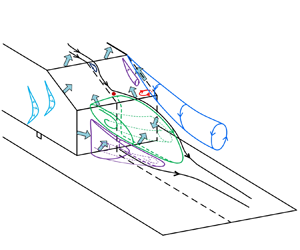
Liu et al. (Reference Liu, Zhang and Zhou2021) carried out a relatively thorough investigation on the flow structures around this body and proposed a conceptual model of the flow structures. Unlike the well-known classical flow structure model developed by Ahmed et al. (Reference Ahmed, Ramm and Faltin1984), which is constructed based on time-averaged data, Liu et al.'s (Reference Liu, Zhang and Zhou2021) model embraces both steady and unsteady coherent structures around the body and even the predominant frequencies of the unsteady structures. Based on this model, five different actuations based on constant blowing, referred to as C 1, C 2, C 3, C 4 and C 5 (figure 2a), were deployed. C 1, C 3 and C 5 are three arrays of microjets along the upper and lower edges of the slanted surface and the lower edge of the base, respectively, each array consisting of 45 circular orifices of 1 mm diameter; C 2 and C 4 each comprise two microjet arrays, arranged along the two side edges of the rear window and the vertical base, respectively, each array includes 28 orifices for C 2 and 15 for C 4. The separation between two neighbouring orifices is the same, 2 mm, for all actuations. The blowing angle θCi of Ci (i = 1, 2, …, 5) may change via replacing the actuator, each fabricated with a different θCi. Three blowing angles of 0°, 55°and 120° were tested for DR for each of C 1 and C 3, and angles of 30°, 90° and 150° for each of C 2 and C 4; C 5 was examined at θC 5 = −45°, 0° and 45°.
(a) Arrangement of actuations on the rear window and the vertical base of the Ahmed body and the definitions of the blowing angles, where θC 3 and θC 5 are positive and negative, respectively. (b) Top and side views of the chamber. Measurement locations of surface pressure on (c) the rear window and (d) the vertical base. The length unit is mm.

Each array of microjets is associated with a separate chamber (figure 2b), embedded in the model. The chamber is connected to supply air via a flexible tube through the hollow strut of the model. The tube is hanging vertically downward from the model before reaching the ground, so that the resultant horizontal force between the tube and the ground is negligibly small. The chamber inlet consists of 6 equally separated holes of 8 mm diameter for C 1, C 3 and C 5, and 3 and 2 holes for C 2 and C 4, respectively. Air flows into the chamber along streamlined diverging passages before reaching the outlet, which act to minimize the non-uniformity of the microjets through the orifices. The flow rate through the chamber is measured and controlled using a mass flow controller (Flow Method FL-805) with a measuring range of 0–200 l min−1 and an uncertainty of ±2 l min−1. The blowing ratio BRCi is defined by
 \begin{equation}\begin{array}{*{20}{c}} {B{R^{Ci}} = \dfrac{{{V_{Ci}}}}{{{U_\infty }}},} \end{array}\end{equation}
where VCi is the exit velocity of a microjet. Figure 3 presents the distributions of the time-averaged centreline velocity  $\overline {{V_c}} $ along the jet exit for each of the five actuations (C 1, C 2, C 3, C 4 and C 5). This velocity was measured using a Pitot static tube connected to an electronic manometer (Furness FCO560) 1 mm downstream of the jet exit. The value of $\overline {{V_c}} $ exhibits a very small variation, <2 % of $\overline {{V_c}} $, from one microjet to another, irrespective of Ci (i = 1, 2, …, 5).
Distributions of  $\overline {{V_c}} $ along each microjet array measured at 1 mm above the centre of the jet exit: C 1 (θC 1 = 55°), $C_\mu ^{C1} = 0.081$; C 2 (θC 2 = 90°), $C_\mu ^{C2} = 0.051$; C 3 (θC 3 = 55°), $C_\mu ^{C3} = 0.056$; C 4 (θC 4 = 90°), $C_\mu ^{C4} = 0.006$; C 5 (θC 5 = 0°), $C_\mu ^{C5} = 0.016$.

2.2. Flow measurements
A single hot-wire was placed along the y-direction to measure the velocity fluctuations uxz in the (x, z) plane to detect the predominant frequencies in the wake. The sensing element was a tungsten wire 5 μm in diameter and approximately 1 mm in length. The wire was operated on a constant temperature circuit (Dantec Streamline) at an overheat ratio of 1.8. The signal from the wire was offset, amplified and low-pass filtered at a cutoff frequency of 1.0 kHz, and digitized at a sampling frequency fs of 6 kHz using a 16-bit A/D converter (NI PCI-6143). Hot-wire measurements were performed at x* = 0.8, y* = 0 and z* = 0. The sampling duration was 60 s, producing a total of 3.6 × 10⁵ data for each record. At least three records were obtained for each test configuration. A fast Fourier transform (FFT) algorithm was used to calculate the power spectral density function Eu of uxz, which is normalized by the variance of uxz so that its integration over the entire frequency range is unity. The FFT window size Nw was 4096. The frequency resolution Δf in the spectral analysis depends on fs and Nw, viz. Δf = fs/Nw (e.g. Zhou et al. Reference Zhou, Du, Mi and Wang2012) = 1.46 Hz.
A LaVision planar PIV system was used to measure the wake of the Ahmed model. The model surface, raised floor and tunnel working section walls were all painted black to minimize laser reflection. The flow was seeded with Di-Ethyl-Hexyl-Sebacat tracer particles approximately 1 μm in diameter. Flow illumination was provided by two standard pulsed laser sources (Vlite-200) of 532 nm wavelength, each with a maximum energy output of 200 mJ per pulse. Each laser pulse lasted for 0.01 μs. One charge-coupled device (CCD) camera (Imager pro HS4M, 4-megapixel sensors, 2016 × 2016 pixels resolution) was used to capture particle images. Synchronization between image taking and flow illumination was provided by the LaVision timer box. The PIV measurements were performed in the (x, z) planes at y* = 0 (symmetry plane) and 0.36, the (x, y) plane of z* = 0.24 and 0.67 and the (y, z) plane at x* = −0.09 and 0.43. The PIV images covered an area of x* = −0.95 to 1.5 and z* = −0.74 to 1.71 in the (x, z) planes, x* = −0.61 to 1.74 and y* = −1.12 to 1.23 in the (x, y) planes and y* = −0.92 to 0.91 and z* = −0.23 to 1.6 in the (y, z) planes. The image magnifications in both directions of each plane were identical, approximately 203, 195 and 152 μm pixel−1 in the (x, z), (x, y) and (y, z) planes, respectively. The intervals between two successive pulses were 90 μs, 80 μs and 20 μs for measurements in the (x, z), (x, y) and (y, z) planes, respectively. In processing the PIV images, the adaptive PIV method was used with a minimum interrogation area size of 32 × 32 pixels and a maximum size of 64 × 64 pixels. The grid step size of 16 × 16 pixels produced 126 × 126 in-plane velocity vectors and the same number of vorticity data points ωx, ωy or ωz.
Following Zhang et al. (Reference Zhang, Liu, Zhou, To and Tu2018) and Liu et al. (Reference Liu, Zhang and Zhou2021), the uncertainty of PIV measurements was evaluated based on image matching analysis. This approach identifies particle image pairs in two successive exposures according to the measured displacement vectors, and evaluates the residual distance or particle disparity between the particle image pairs, which dictates the uncertainty of velocity measurements. Further details of this technique can be found in Sciacchitano, Wieneke & Scarano (Reference Sciacchitano, Wieneke and Scarano2013). In the (x, z) planes of y* = 0 and 0.36, the root-mean-square (r.m.s.) value of the disparity was found to be approximately 0.05 pixel in both the x and z directions, resulting in the uncertainties,  ${\sigma _U}$ and ${\sigma _W}$, in U and W of 0.7 %U∞. The r.m.s. values of the disparity were found to be 0.05 pixel in the (x, y) planes of z* = 0.24 and 0.67, and 0.04 pixel in the (y, z) planes of x* = −0.09 and 0.43. The uncertainties ( ${\sigma _U}$ and ${\sigma _V}$) of U and V in the (x, y) planes are estimated to be approximately 0.9 %U∞, and those ( ${\sigma _V}$ and ${\sigma _W}$) in the (y, z) planes are approximately 2 %U∞. A total of 1800 images were captured for each test run, with a trigger rate of 15 Hz in the double frame mode. The percentage variations of ${\bar{U}^\ast }$, ${\bar{V}^\ast }$, ${\bar{W}^\ast }$, $\bar{\omega }_x^\ast $, $\bar{\omega }_y^\ast $ or $\bar{\omega }_z^\ast $ converge with an increasing number of images to less than ±1 % once the image number exceeds 1200, irrespective of the measurement plane or trigger rate. As such, 1800 images are considered to be adequate for capturing the mean and fluctuating flow fields.
2.3. Aerodynamic drag and surface pressure measurements
Time-averaged aerodynamic drag was measured using a six-component force balance (China Academy of Aerospace Aerodynamics, HGDDS-80), which is accurate to 0.01 N. The balance was mounted on a rigid frame fixed directly onto the ground surface in order to minimize the effect of wind tunnel vibration on measurements (figure 1a). The test model was rigidly mounted on the balance via the four hollow cylindrical posts 280 mm in height, which were fixed to a horizontal connecting plate that was screwed onto the balance. The posts were isolated from the raised floor and the wind tunnel, and were enclosed by a sealed compartment between the raised floor and the bottom wall of the tunnel test section, to avoid the force transmission and the effect of aerodynamic forces resulting from the gap flow on measurements. Without sealing the compartment, the drag force induced by the flow between the raised floor and the bottom wall on each cylindrical support is estimated to be approximately 0.22 N, approximately 18 % of the drag on the Ahmed body, given a flow velocity of 15 m s−1. The sampling frequency was 1 kHz for the drag force measurement with a duration of 60 sec, producing a total of 6 × 10⁴ samples for each record. At least three records were collected for each test configuration.
Following Littlewood & Passmore (Reference Littlewood and Passmore2012), the aerodynamic drag FD is given by the force-balance-measured drag  ${F_x}$ subtracted by the thrust force Fj induced by the blowing jets, viz.
 \begin{equation}{F_D}\; = \; {F_x} - {F_j},\end{equation}
where Fj was obtained at U∞ = 0 m s−1. The drag coefficient CD is calculated by
 \begin{equation}{C_D} = \frac{{{F_D}}}{{0.5\; \rho \; U_\infty ^{\; 2}A}}.\end{equation}
The drag coefficient variation ΔCD is defined by
 \begin{equation}\Delta {C_D} = \frac{{{C_D} - {C_{D0}}}}{{{C_{D0}}}},\end{equation}
where CD 0 is the drag coefficient of the model in the absence of control.
The pressures on the slanted surface and the vertical base were monitored from twenty-six pressure taps (figure 2c,d), which were connected to an electronic pressure scanner (a PSI DTC Initium system) using the plastic tubes of 1 mm inner diameter. The scanner was placed inside the test model to minimize the length of the tubes connected to each tap and hence to limit the filtering effect of tubing in pressure measurements (Grandemange et al. Reference Grandemange, Mary, Gohlke and Cadot2013). The measurement uncertainty is estimated to be ±1 Pa. At least three test runs were conducted for each flow condition. The sampling duration is 60 s, with a fs of 650 Hz, for pressure measurements. The instantaneous pressure coefficient Cpi is given by
 \begin{equation}{C_{pi}} = \frac{{{p_i} - {p_0}}}{{0.5\rho U_\infty ^2}},\quad i \in \{ 1,2, \ldots ,26\} ,\end{equation}
where pi is the instantaneous local pressure and p 0 is the free-stream static pressure (=45 Pa at U∞ = 15 m s−1) measured at x* = −4.9, y* = 0 and z* = 3.1 above the leading edge of the raised floor. The change  $\Delta \overline {{C_{pi}}} $ of the time-averaged local pressure coefficient is given by
 \begin{equation}\Delta \overline {{C_{pi}}} \; = \frac{{\overline {{C_{pi}}} - \overline {{C_{pi0}}} }}{{|\overline {{C_{pi0}}} |}},\end{equation}
where Cpi 0 is the instantaneous pressure coefficient in the baseline flow. The spatially averaged pressure coefficients on the rear window  $({\langle \overline {{C_p}} \rangle _r})$ and the vertical base $({\langle \overline {{C_p}} \rangle _b})$ are calculated by
 \begin{equation}{\langle \overline {{C_p}} \rangle _r}\; = \; \frac{{\displaystyle\sum\limits_{i = 1}^{13} {\overline {{C_{pi}}} } }}{{13}},\end{equation}
and
 \begin{equation}{\langle \overline {{C_p}} \rangle _b}\; = \; \frac{{\displaystyle\sum\limits_{i = 14}^{26} {\overline {{C_{pi}}} } }}{{13}}.\end{equation}
 The contribution of  ${\langle \overline {{C_p}} \rangle _r}$ and ${\langle \overline {{C_p}} \rangle _b}$ to the force along the drag direction can be expressed by
 \begin{equation}\langle \overline {{C_p}} \rangle \; = \; \frac{{{{\langle \overline {{C_p}} \rangle }_r}\; \sin (\varphi ) + {{\langle \overline {{C_p}} \rangle }_b}}}{2}.\end{equation}
Then, the change of  $\langle \overline {{C_p}} \rangle$ is given by
 \begin{equation}\Delta \langle \overline {{C_p}} \rangle = \frac{{\langle \overline {{C_p}} \rangle - \langle \overline {{C_{p0}}} \rangle }}{{|\langle \overline {{C_{p0}}} \rangle |}},\end{equation}
where  $\langle \overline {{C_{p0}}} \rangle $ is the effective spatially averaged pressure coefficient in the absence of control. The negative or positive sign of $\Delta \langle \overline {{C_p}} \rangle $ represents a drop or rise in pressure.
The aerodynamic drag measurements were carried out at U∞ from 7.5 to 24 m s−1, corresponding to the Re range of (0.9–2.7) × 105 based on  $\sqrt A $ and U∞, and all other measurements were performed at U∞ = 15 m s−1 (Re =1.7 × 10⁵).
3. AI Control based on ACA
3.1. AI control system and cost function design
The AI control system sketched in figure 4(a) consists of a plant, a sensing unit (pressure taps), an execution unit and a control logic/controller, as in Zhou et al. (Reference Zhou, Fan, Zhang, Li and Noack2020). The control logic provides the execution unit with instructions or commands, and the latter, i.e. the independently operated microjet arrays, then executes, which manipulates the control plant (the flow around the Ahmed body). The real-time control command is generated by a National Instrument PXIe-6356 multifunction I/O device, connected to a computer. A LabVIEW Real-Time module is used to execute the command. The sensing unit monitors the plant output and processes the information from the pressure taps, based on which a decision will be made on whether the control goal has been achieved. If yes, stop; otherwise, continue the search for the optimal control parameters. The execution hardware and control logic are intimately interwoven, facilitating achieving of the control goal of the plant. Before introducing the control logic in § 3.2, we discuss the set-up of the control goal, i.e. the design of the cost function J.
(a) Sketch of the principle of the AI control system, which comprises the plant, sensors, actuators and an ACA controller. (b) Schematic of ant colony optimization algorithm.

Aiming to find efficient control strategies, which may achieve a substantial DR at small expenses, i.e. small control power input, we define J by
 \begin{equation}J ={-} \langle \overline {{C_p}} \rangle + {\beta _p},\end{equation}
where  $- \langle \overline {{C_p}} \rangle$ provides a measure for the estimate of drag (Li et al. Reference Li, Noack, Cordier, Borée and Harambat2017; Fan et al. Reference Fan, Zhang, Zhou and Noack2020a) and βp is the penalization term connected to the control power input, given by
 \begin{equation}{\beta _p}\; = \; \alpha \sum\limits_{i = 1}^5 {{{(B{R^{Ci}})}^3}} .\end{equation}
In (3.2), α is a weighting factor. Following the energy input analyses by Wassen & Thiele (Reference Wassen and Thiele2010), Barros et al. (Reference Barros, Borée, Noack and Spohn2016) and Zhang et al. (Reference Zhang, Liu, Zhou, To and Tu2018), the power input of Ci (i = 1, 2, …, 5) may be calculated by
 \begin{equation}{P_{Ci}} = 0.5{N_{Ci}}\rho {A_{Ci}}U_\infty ^{\; 3}{(B{R^{Ci}})^3},\end{equation}
where NCi is the number of microjets, and ACi is the exit area of a microjet. The choice of α is twofold. First, α is such that the penalization term plays an appreciable role in control; second, α cannot be too large to dominate J (Raibaudo et al. Reference Raibaudo, Zhong, Noack and Martinuzzi2020). The present α is set at 0.00002 so that the penalization term is between 0.04 % and 9 % of  $ - \langle \overline {{C_{p0}}} \rangle $ when BRCi increases from 1 to 6 for each actuation. The variation in J is given by
 \begin{equation}\Delta J = \frac{{J - {J_0}}}{{{J_0}}},\end{equation}
where J 0 is the cost for the baseline flow.
3.2. Optimization algorithm based on ACA
In the present control system, there are five control parameters, i.e. BRC 1, BRC 2, BRC 3, BRC 4 and BRC 5, to be optimized. It becomes challenge for conventional optimization techniques once the number of control parameters exceeds three; for instance, the extremum seeking method based on extended Kalman filter could be applied to at most three control parameters (Fan, Zhou & Noack Reference Fan, Zhou and Noack2020b). On the other hand, the AI control may get around this difficulty and may find the global optimum solution even when the number of control parameters is rather large, as demonstrated by Zhou et al. (Reference Zhou, Fan, Zhang, Li and Noack2020).
The ACA is presently used. Inspired by the behaviour of ant colonies in nature, Dorigo et al. (Reference Dorigo, Maniezzo and Colorni1991) proposed an approach for solving hard combinatorial or discrete problems. In their work, the well-known travelling salesman problem was used as an application example, and the ACA was found to be effective in finding out the optimal or shortest tour. The ACA uses many interacting agents, called artificial ants mimicking the real ones mediated by pheromone trails, and an algorithm based on positive feedback for exploring rapidly the optimal solution. Liao et al. (Reference Liao, Montes de Oca, Stützle and Dorigo2014) developed a unified framework of ACA, in which the ants in each cycle are divided into two groups, one whose costs are below a threshold, performing a local search near the best ant, and the other executing a global search in the entire parameter space. This method is demonstrated to be efficient in finding the global optimum solutions, when applied to more than 20 benchmark multimodal functions, without being trapped in local minima. They obtained the global extremum for every benchmark function with faster speed and higher accuracy as compared with conventional ACA methods (Dorigo et al. Reference Dorigo, Maniezzo and Colorni1991; Socha & Dorigo Reference Socha and Dorigo2008). This ACA is implemented presently for the first time as an algorithm of MLC in order to find the best control strategy for the DR of an Ahmed body wake, and is briefly introduced below.
The vector B = [b 1, b 2, …, b 5]T comprises all actuation commands or analogue voltages, where the superscript ‘T’ denotes the transpose and bi (i = 1, 2, 3, 4 or 5) regulates the mass flow controller for Ci (figure 4a). Then
 \begin{equation}\boldsymbol{B} = \boldsymbol{K}(\boldsymbol{BR}),\end{equation}
where BR = [BRC 1, BRC 2, …, BRC 5]T is referred to as the control law of the combined actuations in this paper and K is the vector function that transforms BR to the control signals of the mass flow controllers. The optimization process searches for a law of form (3.5) that minimizes the cost:
 \begin{equation}{\boldsymbol{K}_{\boldsymbol{opt}}} = \mathop {\arg \,\min \; }\limits_{\boldsymbol{K}} J[\boldsymbol{K}(\boldsymbol{BR})].\end{equation}
The regression problem is to optimize mapping from five inputs (BRC 1, BRC 2, …, BRC 5) to a single output signal J and the optimizing process is schematically shown in figure 4(b), described briefly below:
Step 1: the process is initialized with a set of M = 100 randomly generated  $\boldsymbol{BR}_{\boldsymbol{m}}^{\boldsymbol{n}}$, m = 1, …, M, also called ants, for the first cycle of ACA (n = 1). Here, the superscripts ‘n’ and ‘m’ denote the cycle number and the mth control command of each cycle.
Step 2: each ‘m’ is experimentally tested for 25 s to yield the measured cost  $J_m^n$. The pheromone $(\tau _m^n)$ is given by
 \begin{equation}\tau _m^n = (1 - {e_v})\tau _m^{n - 1} + J_m^n,\quad (n = 1, \ldots ,N),\end{equation}
where ev is the evaporation rate and is set to 0.9, and N is the total number of cycles. The value of  $\tau _m^0$ is zero. Then, the ants are renumbered in order of the pheromone values, $\tau _1^n < \tau _2^n < \cdots < \tau _M^n$.
Step 3: the ants are sorted into two groups, one performing a local search, and the other regenerated randomly in the entire search space. The transition probability  $(P_m^n)$ for the local search is written as
 \begin{equation}P_m^n = \left\{ {\begin{array}{@{}ll} 1&{p_m^n\; < \; {p_0}}\\ 0&{p_m^n\; \ge \; {p_0}} \end{array}} \right.,\end{equation}
where  ${p_0}$ is a threshold, which affects largely the ratio of ants that perform local or global searches. A right choice of ${p_0}$ may raise the efficiency of the global searching of the ACA, ensuring a relatively large number of ants to be generated randomly in the entire search space (or global searching). Otherwise, most ants may get engaged in local searching. The ${p_0}$ is presently chosen to be 0.2 after a trial-and-error process. The $p_m^n$ is a variation in $\tau _m^n$ relative to $\tau _1^n$, viz.
 \begin{equation}p_m^n\; = \; \frac{{\tau _m^n - \tau _1^n}}{{\tau _1^n}}.\end{equation}
The ant conducting the local search is determined by
 \begin{equation}\boldsymbol{BR}_{\boldsymbol{m}}^{\boldsymbol{n}{\bf + 1}} = \boldsymbol{BR}_{\boldsymbol{m}}^{\boldsymbol{n}} + \frac{1}{{2n}}{\boldsymbol{R}_{\boldsymbol{a}}},\quad {\boldsymbol{R}_{\boldsymbol{a}}} = {[{r_1},{r_2}, \ldots ,{r_5}]^\textrm{T}},\end{equation}
where ri (i = 1, 2, …, 5) can be expressed by
 \begin{equation}{r_i} = 2{S_i}[\textrm{rand}(0,\; 1) - 0.5],\end{equation}
and Si denotes the maximum BRCi for Ci.
Step 4: next cycle starts with step 2 until the cost is converged to its minimum.
4. Results and discussion
4.1. Base flow characterization
The base flow of the Ahmed body is first documented. Its drag coefficient CD 0 drops from 0.36 to 0.29 with increasing Re from 0.9 × 10⁵ to 2.7 × 10⁵. The uncertainty in CD 0, given by  $\overline {\overline {|{C_{D0}} - \overline {\overline {{C_{D0}}}} |}}$, where the double overbar denotes averaging over three test runs (Bidkar et al. Reference Bidkar, Leblanc, Kulkarni, Bahadur, Ceccio and Perlin2014), is estimated to be between 0.0005 and 0.004, one order of magnitude smaller than the drop (0.07) in CD 0. The measured CD 0 and its variation agree well with previous reports on an Ahmed body with φ = 35° by Ahmed, Ramm & Faltin (Reference Ahmed, Ramm and Faltin1984), Guilmineau (Reference Guilmineau2008), Meile et al. (Reference Meile, Ladinek, Brenn, Reppenhagen and Fuchs2016) and Liu et al. (Reference Liu, Zhang and Zhou2021), who observed a decline in CD 0 from 0.32 to 0.26 from Re = 1.7 × 10⁵ to 1.4 × 10⁶.
Figure 5(a) presents the time-averaged sectional streamlines superimposed over the in-plane velocity magnitude  ${\overline {{U_{xz}}} ^\ast }$ in the symmetry plane of the wake. Hereinafter, the sectional streamlines are referred to as streamlines for simplicity. Flow separates from the upper edge of the rear window and the lower edge of the vertical base and then rolls up, forming two recirculation bubbles, one above the other (e.g. Lienhart & Becker Reference Lienhart and Becker2003; Liu et al. Reference Liu, Zhang and Zhou2021). The upper bubble is much bigger than the lower one, covering both the rear window and most of the upper part of the base, which is highlighted by the thick solid contour in figure 5(a). The streamlines may allow us to determine the length of the recirculation bubbles, defined by the maximum longitudinal bubble length of $\bar{U} \le 0$ (e.g. Zhang, Zhou & To Reference Zhang, Zhou and To2015). The length $(l_{u0}^\ast )$ of the upper recirculation bubble is approximately 0.98. The lower bubble is hardly discernible in the streamlines, probably because of a jittering in this bubble during time averaging (Liu et al. Reference Liu, Zhang and Zhou2021). Within the upper bubble, the upwash flow near the base separated from the upper edge of the base and then rolled up under the pressure difference between the flow at the base and that over the rear window, generating a corner vortex. This vortex accounts for the anti-clockwise rotation of streamlines near the lower edge of the slanted surface (figure 5a).
(a) Time-averaged streamlines superimposed with the contours of velocity magnitude  ${\overline {{U_{xz}}} ^\ast }$ and (b) $\bar{\omega }_y^\ast $-contours in the symmetry plane (vorticity contour interval = 1). (c) Time-averaged streamlines superimposed with the contours of velocity magnitude ${\overline {{U_{yz}}} ^\ast }$ and (d) $\bar{\omega }_x^\ast $-contours in the (y, z) plane of x* = −0.09 (vorticity contour interval = 0.5). Thick purple closed contours correspond to the time-averaged swirling strength ${\overline {\lambda _{ci}^2} ^\ast } = 0.1$ and 0.02 in (b) and (d), respectively. Flow is unforced.

The vortex definition proposed by Zhou et al. (Reference Zhou, Adrian, Balachandar and Kendall1999), which is briefly introduced below, is adopted for the identification of vortices from the vorticity data. A vortex core is a region where the velocity gradient tensor  $\boldsymbol{\nabla }\boldsymbol{U}$ has complex eigenvalues (Chong, Perry & Cantwell Reference Chong, Perry and Cantwell1990). Then, $\boldsymbol{\nabla }\boldsymbol{U}$ may be written as
 \begin{equation}\boldsymbol{\nabla
}\boldsymbol{U} = \left[ {\begin{array}{@{}ccc@{}}
{{\boldsymbol{v}_r}}&{{\boldsymbol{v}_{cr}}}&{{\boldsymbol{v}_{ci}}}
\end{array}} \right]\left[ {\begin{array}{@{}ccc@{}}
{{\lambda_r}}&{}&{}\\
{}&{{\lambda_{cr}}}&{{\lambda_{ci}}}\\ {}&{ -
{\lambda_{ci}}}&{ - {\lambda_{cr}}} \end{array}}
\right]{\left[ {\begin{array}{@{}ccc@{}}
{{\boldsymbol{v}_r}}&{{\boldsymbol{v}_{cr}}}&{{\boldsymbol{v}_{ci}}}
\end{array}} \right]^{ -
1}},\end{equation}
\begin{equation}\boldsymbol{\nabla
}\boldsymbol{U} = \left[ {\begin{array}{@{}ccc@{}}
{{\boldsymbol{v}_r}}&{{\boldsymbol{v}_{cr}}}&{{\boldsymbol{v}_{ci}}}
\end{array}} \right]\left[ {\begin{array}{@{}ccc@{}}
{{\lambda_r}}&{}&{}\\
{}&{{\lambda_{cr}}}&{{\lambda_{ci}}}\\ {}&{ -
{\lambda_{ci}}}&{ - {\lambda_{cr}}} \end{array}}
\right]{\left[ {\begin{array}{@{}ccc@{}}
{{\boldsymbol{v}_r}}&{{\boldsymbol{v}_{cr}}}&{{\boldsymbol{v}_{ci}}}
\end{array}} \right]^{ -
1}},\end{equation}
where λr is the real eigenvalue with a corresponding eigenvector vr, and λcr ± λcii is a conjugate pair of the complex eigenvalues with eigenvectors vcr ± vcii. The local flow is either stretched or compressed along the axis vr, while swirling in the plane determined by vectors vcr and vci. The local swirling strength of the vortex is given by the imaginary part of the complex eigenvalue pair λci. This method is independent of the reference frame and would not detect regions containing significant vorticity such as shear layers but no local swirling motion. A vortical motion is identified if  $\lambda _{ci}^{2\ast }$ is larger than a threshold, approximately 3 % of the maximum $\lambda _{ci}^{2\ast }$, which is 0.100 in the (x, z) planes of y* = 0 and 0.36 and the (x, y) planes of z* = 0.24 and 0.67, and 0.020 and 0.001 in the (y, z) planes of x* = −0.09 and 0.43, respectively.
The  $\bar{\omega }_y^\ast $ contours in the symmetry plane (figure 5b) display an upper negative-signed concentration and a lower positive-signed concentration, both spatially coinciding with purple-coloured thick solid contours of $\lambda _{ci}^{2\ast } = 0.1$. Obviously, the two vorticity concentrations are associated with the two recirculation bubbles in the wake. Furthermore, one positive $\bar{\omega }_y^\ast $ concentration with $\bar{\omega }_{y,max}^\ast = 3.6$ occurs at the lower edge of the rear window, which is ascribed to the corner vortex. Hereinafter, subscripts ‘max’ and ‘min’ denote the maximum vorticity concentrations of positive and negative signs, respectively.
Figure 5(c,d) presents time-averaged streamlines and the  $\bar{\omega }_x^\ast $ contours in the (y, z) planes of x* = −0.09 (above the rear window). The flow exhibits several features. First, a downwash flow occurs above z* ≈ 0.76, which is linked to flow separation from the roof. Second, an upwash flow takes place at z* from 0.61 to 0.76, which is associated with the upstream and upward motion of flow from the base to the rear window within the upper recirculation bubble, as is evident from the streamlines in the (x, z) plane of y* = 0 (figure 5a). Third, a flow moves toward the slanted surface below z* ≈ 0.61, which is connected to the reattachment of the flow separated from the upper edge of the base. As shown in the $\bar{\omega }_x^\ast $ contours (figure 5d), two concentrations marked by ‘C’, the signatures of the well-known C-pillar vortices, occur behind the two side edges of the rear window, whose maximum magnitude reaches approximately 2.1 at (y*, z*) ≈ (±0.53, 0.83), resulting from a swirling motion. This motion is the rollup of shear layer coming off the sidewall about the side edge of the slanted surface, due to a pressure difference between flow at the sidewall and that over the rear window (Ahmed et al. Reference Ahmed, Ramm and Faltin1984). The C-pillar vortices are much weaker in strength than their counterparts in the high-drag regime (e.g. Hucho & Sovran Reference Hucho and Sovran1993); the maximum $\bar{\omega }_x^\ast $ of the former is ten times larger than that of the latter based on the PIV data measured in the (y, z) plane of x* = 0.2 (Wang et al. Reference Wang, Zhou, Pin and Chan2013). A number of alternately signed $\bar{\omega }_x^\ast $ concentrations occur near the rear window. The C-pillar vortex may induce an inboard neighbouring vorticity concentration or a secondary vortex with an opposite sign (Zhang et al. Reference Zhang, Zhou and To2015). For the same reason, this secondary vortex may induce another $\bar{\omega }_x^\ast $ concentration next to it.
4.2. Combined actuations
4.2.1. Optimization of control parameters based on ACA algorithm
The control performance under individual C 1, C 2, C 3, C 4 and C 5 is first investigated. Figure 6 shows the dependence of ΔCD on the blowing ratio for the five individual actuations operated at different blowing angles. The uncertainty of ΔCD is estimated to be within 1 %. It can be seen that the blowing angle produces a significant effect on the DR performance. Firstly, the drag can be either substantially decreased or increased by C 1, depending on θC 1 (figure 6a). At θC 1 = 0°, the drag drops with increasing blowing ratio, the maximum DR being approximately 9 % when BRC 1 reaches 5.7. Beyond this BRC 1, the drag grows. On the other hand, the drag rises with increasing BRC 1 at θC 1 = 55° and 120°, ΔCD reaching 17 % and 29 % at BRC 1 = 6.3, respectively. Secondly, when C 2 is operated at θC 2 = 30°, BRC 2 produces little influence on the drag (figure 6b). This is not the case at θC 2 = 90°and 150° where the drag increases by 16 % and 51 % at BRC 2 = 9.1, respectively. Thirdly, there appears one critical blowing ratio  $BR_{cr}^{C3} = 1.9$ under C 3 (figure 6c), regardless of θC 3; the drag drops initially, reaching its minimum at $B{R^{C3}} = BR_{cr}^{C3}$, and then rises with increasing BRC 3. The maximum DRs are 2 %, 3 % and 5 % for θC 3 = 0°, 55°and 120°, respectively. Fourthly, like C 2, C 4 achieves little DR at θC 4 = 30° (figure 6d). Finally, C 5 achieves its maximum DRs of 2 % and 7 % at BRC 5 = 2.5 for θC 5 = 0° and 45°, respectively (figure 6e), but no DR for θC 5 = −45°, irrespective of BRC 5. Table 4 shows ${\langle \overline {{C_p}} \rangle _r}$, ${\langle \overline {{C_p}} \rangle _b}$ and $\langle \overline {{C_p}} \rangle $ under each actuation, along with their variations and corresponding DR.
Dependence of the change ΔCD in the drag coefficient on (a) blowing ratios BRC 1, (b) BRC 2, (c) BRC 3, (d) BRC 4 and (e) BRC 5 under individual C 1, C 2, C 3, C 4 and C 5 at various blowing angles (Re = 1.7 × 10⁵). The uncertainty bars of ΔCD are calculated from  $\overline{\overline {|\Delta {C_D} - \overline{\overline {\Delta {C_D}}} |}} $.

Individual C 1, C 2, C 3, C 4 and C 5 may have difficulty in controlling all or most of the predominant coherent structures, thus achieving rather limited DR. The DR under the combinations of C 1 (θC 1 = 0°), C 2 (θC 2 = 30°), C 3 (θC 3 = 120°), C 4 (θC 4 = 30°) and C 5 (θC 5 = 45°) is examined given the same blowing coefficient (Cm) for every actuation, which is defined by
 \begin{equation}{C_m} = \frac{Q}{{{U_\infty }A}},\end{equation}
where Q is the volume flow rate (Fan et al. Reference Fan, Zhang, Zhou and Noack2020a). The dependence of ΔCD on Cm is presented in figure 7. The maximum DR reaches 11 % at Cm = 4.0 × 10⁻³, slightly larger than that (9 %) achieved under individual actuations. One issue arises, that is, can we find a combination of these five actuations so that all the coherent structures can be effectively and simultaneously manipulated, producing a significantly more pronounced DR? In this section, we explore based on the AI control system introduced in § 3.1 the best strategy of the combined actuations for DR at Re = 1.7 × 10⁵.
Spatially averaged pressure coefficients  ${\langle \overline {{C_p}} \rangle _r}$, ${\langle \overline {{C_p}} \rangle _b}$ and $\langle \overline {{C_p}} \rangle $, their variations, and the corresponding DR under C 1 (θC 1 = 0°), C 2 (θC 2 = 30°), C 3 (θC 3 = 120°), C 4 (θC 4 = 30°) and C 5 (θC 5 = 45°).

Dependence of DR on Cm under the combination of C 1, C 2, C 3, C 4 and C 5.

The ACA-based AI system searches for the optimal blowing ratios of all the five actuations. In the learning process, the cost of each ant was tested for 25 s, which is a compromise between the duration for time averaging and the converged cost function or cost. The learning curve of the AI control is presented in figure 8. Each cycle consists of 100 ants, corresponding to 100 costs, which form one colour bar. The square symbol highlights the best ant (An) of a cycle, corresponding to a minimum cost Jn, and the remaining costs of this cycle are arranged monotonously, following an ascending order. The trend shown by the square symbols reveals the evolution of the best ant from cycle n = 1 to 20, and the corresponding control parameters are shown in table 5. Here, A 1 is associated with BR = [6.0, 6.5, 4.3, 1.9, 1.8]T, which produces a cost of J 1 = 0.243. This cost is 3 % higher than J 0 in the absence of forcing;  $\Delta \langle \overline {{C_p}} \rangle $ associated with A 1 is approximately 2 %, corresponding to a DR of 1 %. This is not unexpected in view of (3.1) as βp is relatively large, about 5 % of J 0. J 2 drops substantially by 8 % relatively to J 0, the corresponding $\Delta \langle \overline {{C_p}} \rangle $ and DR being 13 % and 8 %, respectively. In the third cycle, J 3 decreases further to 0.212, with a DR of 9 %. The control parameters of A 4, A 5 and A 6 are unchanged with BR = [6.1, 4.1, 4.6, 2.5, 1.6]T. The maximum deviation in the cost between A 4, A 5 and A 6 is less than 1 %, within the measurement uncertainty, 2 %J 0, of J. A 7 corresponds to BR = [5.4, 3.7, 5.1, 2.1, 2.1]T, yielding a drop in J by 20 % or a DR of 13 %. After that, J 8 drops substantially to 0.166 and remains unchanged for n ≥ 9, implying a convergence of the cost that produces the highest ΔJ of −29 %, that is, the optimal or minimal cost Jopt is achieved. The optimized control law Bopt is [5.8, 3.5, 4.9, 1.3, 1.8]T, yielding an impressive DR of 18 %, significantly higher than any previously reported DR for a low-drag Ahmed body. The maximum DR obtained experimentally so far is only 4 % (Jahanmiri & Abbaspour Reference Jahanmiri and Abbaspour2011).
Learning curve of ACO control for the combined actuations of C 1 (θC 1 = 0°), C 2 (θC 2 = 30°), C 3 (θC 3 = 120°), C 4 (θC 4 = 30°) and C 5 (θC 5 = 45°). Each colour bar consists of 100 values of J in a cycle. The square symbol highlights the smallest J or Jn of the best ant An in the nth cycle.

Control parameters and performances of the best ants Ai (i = 1, 2, …, 20), as marked by square symbols in figure 8.

As shown in Zhou et al. (Reference Zhou, Fan, Zhang, Li and Noack2020), a careful analysis of proximity maps may provide a good picture on the control laws identified and their distributions along with insight into the optimization process. Following Zhou et al. (Reference Zhou, Fan, Zhang, Li and Noack2020) and Fan et al. (Reference Fan, Zhang, Zhou and Noack2020a), the considered ensemble of BRj is represented as data points in the two-dimensional plane of the feature vectors γj = (γj, 1, γj, 2), where j = 1, 2, …, N × M, so that the distance between the feature vectors is an indicator of the difference between the control laws. The r.m.s.-averaged Euclidean distance Mjk (j, k = 1, 2, …, N × M) between BRj and BRk is given by
 \begin{equation}{M_{jk}} = \sqrt {\sum\limits_i^5 {{{\left( {\frac{{BR_j^{Ci} - BR_k^{Ci}}}{{BR_{mx}^{Ci}}}} \right)}^2}} } ,\end{equation}
where the subscript ‘mx’ denotes the maximal BRCi (i = 1, 2, …, 5) in tests. Figure 9 presents the proximity map of the 1000 control laws found in the first 10 cycles in a two-dimensional plane, where the underlying metric between two control laws BRj and BRk is given by D = (Djk), viz.
 \begin{equation}{D_{jk}} = {M_{jk}} + \lambda |J_j - J_k|,\end{equation}
where λ is the penalty coefficient. The parameter λ is chosen so that the maximum actuation distance of Mjk is equal to the maximum difference in the performance terms. The classical multi-dimensional scaling (Cox & Cox Reference Cox and Cox2001) is used to determine γ 1 and γ 2 for the matrix D so that the length of a feature vector or distance between different control laws can be preserved, yielding
 \begin{equation}\sum\limits_{j = 1}^{N \times M\; } {\sum\limits_{k = 1}^{N \times M\; } {{{(||{\gamma _j} - {\gamma _k}||- {D_{jk}})}^2}} } = min,\end{equation}
where min denotes the minimum value. Control landscape or proximity map is constructed from the three-dimensional data points (γj, 1, γj, 2, Jj), j = 1, 2, …, N × M. An unstructured grid from the Delaunay triangulation is used to connect the two-dimensional feature vectors (Kaiser et al. Reference Kaiser, Noack, Spohn, Cattafesta and Morzyński2017). The J-values in each mesh triangle j 1, j 2, j 3 ∈ {1, …, N × M} are interpolated from the known values at the vertices Jj 1, Jj 2, Jj 3. For n = 1, the best ant occurs at (γ 1, γ 2) = (0, −0.09). As n increases, An is seen to move toward its optimum, reaching A 8 at (γ 1, γ 2) = (−0.24, 0.12). The searching path from A 1 to A 8 follows a rather straight line, indicating an effectiveness and efficiency of the ACA in searching the optimal control law. The AI control takes only 800 test runs to find the optimal combination of actuations.
Control landscape produced from the 1000 control laws, each corresponding to a white circle, obtained in the first 10 cycles of the learning process. The yellow circle denotes the best control law of each cycle.

The γ 1 and γ 2 have technically no a priori meaning. However, a careful analysis of the variation in BR with the optimal control performance may cast light upon the sensitivity of the control performance to individual actuations and associated input energies. Figure 10 shows the dependence of the upper and lower limits for BRCi (i = 1, 2, 3, 4 or 5), denoted by  $BR_{upp}^{Ci}$ and $BR_{low}^{Ci}$, respectively, on a small departure of J from its optimal value Jopt, say Jopt +δ, Jopt +2δ and Jopt +3δ, where δ = 0.01Jopt. This dependence may indicate whether the lowest J or optimal control is sensitive to BRCi. Then, the maximal interval of BRCi is given by
 \begin{equation}\Delta B{R^{Ci}} = BR_{upp}^{Ci} - BR_{low}^{Ci}.\end{equation}
A small change in BRC 1 from 5.9 to 5.0 may lead to a deteriorated J from Jopt to Jopt +δ. The range grows substantially to BRC 1 from 4.0 to 6.0 as J is relaxed from Jopt to Jopt +2δ. When J is further relaxed to Jopt – (Jopt +3δ), the BRC 1 range grows to 2.8–6.0. A similar trend of the blowing ratio range is also observed for BRCi (i = 2, 3, 4 or 5). The observation suggests that a small sacrifice in J may lead to a substantial reduction in BRCi or saving in the input energy. The ΔBRC 1 is approximately 0.9 from Jopt to Jopt +δ, which is comparable to ΔBRC 5 (1.0) but is appreciably smaller than ΔBRC 2 (1.5), ΔBRC 3 (2.2) or ΔBRC 4 (1.4). The ΔBRC 3 is the largest, exceeding 2ΔBRC 1 or 2ΔBRC 5. The results indicate that the DR, when approaching its maximum, is less sensitive to BRC 3 than the other four blowing ratios. A relaxation in J from Jopt to Jopt +2δ leads to a moderate increase in ΔBRCi (i = 1, 2, …, 5) from 0.9, 1.5, 2.2, 1.4 and 1.0 to 2.0, 3.2, 3.5, 2.8 and 2.0, respectively. When this relaxation is further raised to Jopt +3δ, ΔBRC 1 and ΔBRC 5 rise to 3.2 and 2.8, respectively; however, ΔBRC 2, ΔBRC 3 and ΔBRC 4 grow more significantly to 6.4, 4.3 and 4.2, respectively, ΔBRC 2 being the largest. The observation implies that the near-optimal control is quite sensitive to BRC 1 and BRC 5, but less so to BRC 2, BRC 3 or BRC 4. It seems plausible that one way to enhance the control efficiency is to reduce to a certain extent the power input of control while maintaining a near-maximum DR. Evidently, being sensitive to the maximum DR, BRC 1 and BRC 5 should be kept near their optimal values in order to maximize the DR. On the other hand, we may reduce BRC 2, BRC 3 or BRC 4, without sacrificing much the DR, for the purpose of a rather substantial saving in the power input.
Dependence of the upper and lower limits for BRCi (i = 1, 2, 3, 4 or 5) on a small departure of J from its optimal value Jopt, i.e. Jopt +δ, Jopt +2δ and Jopt +3δ, where δ = 0.01Jopt.

4.2.2. Control efficiency
The active control requires energy input to produce DR. Therefore, it is important to determine the ratio of the power saved from the DR to the control input power  ${P_{Ci}}$ (i = 1, 2, … 5) which is an important indicator to evaluate the efficiency of the control (Choi, Jeon & Kim Reference Choi, Jeon and Kim2008). The control efficiency η is defined by
 \begin{equation}\eta \; = \; \frac{{\Delta {F_D}{U_\infty }}}{{\displaystyle\sum\limits_{i = 1}^5 {{P_{Ci}}} }},\end{equation}
where ΔFD denotes the decrease in drag under control (e.g. Choi et al. Reference Choi, Jeon and Kim2008; Zhang et al. Reference Zhang, Liu, Zhou, To and Tu2018) and  ${P_{Ci}}$ may be calculated from (3.3). From (4.7), the power saved from reduced drag exceeds the control input power if η exceeds unity.
Figure 11 presents the dependence of η on individual blowing ratios for C 1 (θC 1 = 0°), C 2 (θC 2 = 30°), C 3 (θC 3 = 120°), C 4 (θC 4 = 30°) and C 5 (θC 5 = 45°). For all actuations, the maximum η occurs at small BR and then declines continuously with increased BR. At BR ≈ 0.6, η reaches approximately 2.6, 31.8 and 4.5 under C 1, C 3 and C 5, respectively. Nevertheless, η becomes smaller than unity when BRC 1, BRC 2 and BRC 3 exceed 1.3, 2.5 and 3.1, respectively, that is, the power saved from reduced drag is less than the control input power. On the other hand, the maximum η is only 0.2 and 0.6 for C 2 and C 4, respectively, indicating inefficient controls.
(a) Dependence of the control efficiency η on BR under individual C 1, C 2, C 3, C 4 and C 5. (b) Zoom in plot for 0 < η < 6. The uncertainty bars of η are calculated by  $\overline{\overline {|\Delta {F_D} - \overline{\overline {\Delta {F_D}}} |}}\ {U_\infty }/\sum\nolimits_{i = 1}^5 {{P_{Ci}}}$.

To gain an overall picture on how DR and η vary with increasing n and how they could be connected to each other, let us examine the proximity maps (figure 12) of control laws for cycles 1, 7, 12 and 15 along with the normalized control power input, viz.
 \begin{equation}P_c^\ast = \frac{{\displaystyle\sum\limits_{i = 1}^5 {{P_{Ci}}} }}{{{U_\infty }{F_D}}}.\end{equation}
Note that the J-contours in the figure are generated from 2000 control laws in 20 cycles. The diameter of white circles in the figure indicates the magnitude of  $P_c^\ast $. There appears a correlation between the level of J and γ 1; the former displays in general a growth with the latter increasing. However, γ 2 correlates with neither J nor $P_c^\ast $. The control laws occur largely in the right half of the phase plane in the first cycle; they shift gradually toward the left or the negative γ 1 direction and take place within a narrower range of γ 1 with increasing n. The learning process is converged at n = 8 in terms of J when the maximum DR (18 %) is obtained. This maximum is, however, associated with a very small η, only 0.13. However, with n increasing further, both DR and the corresponding η continue to evolve in spite of a negligible change in J. Define En (n = 1, 2, …, 20) as the control law with the highest η in the nth cycle; E 7 corresponds to BR = [0.7, 0.4, 0.5, 0.7, 0.6]T with $P_c^\ast = 0.004$, producing a large η of 25.7 and a DR of 10 %. As the present cost contains the control power input (3.1), there is an overall decline in $P_c^\ast $ with increasing n; for example, the largest $P_c^\ast $ drops from 11.9 in n = 12 to 6.7 in n = 15. Accordingly, η is 1.1 for E 12 (BR = [2.6, 2.6, 0.2, 0.2, 0.3]T) and 5.8 for E 15 (BR = [1.9, 0.3, 0.2, 0.5, 0.5]T), their corresponding DR being 16 % and 15 %, respectively. The latter requires less than 20 % of input energy consumed by the former with a sacrifice in DR by only 1 %. One may surmise that the physical mechanisms must differ between the cases of a pronounced DR but a small η and a less pronounced DR but a substantially increased η, which will be discussed in the next two subsections.
Control landscape associated with cycles 1, 7, 12 and 15 (100 ants for each cycle). The contours of J are produced from 2000 control laws in 20 cycles. Each circle represents a control law, whose diameter is proportional to the power input  $\sum\nolimits_{i = 1}^5 {{P_{Ci}}} /{U_\infty }{F_{D0}}$.

Jahanmiri & Abbaspour (Reference Jahanmiri and Abbaspour2011) attained a DR of only 4 % with a relatively large η of 62.1, who deployed a combination of steady suction near the upper edge of rear window and steady blowing at the mid-height of the base of a low-drag Ahmed body with φ = 45°. Edwige et al. (Reference Edwige, Eulalie, Gilotte and Mortazavi2018) obtained a DR of 2 % with a η of 7.6, who applied pulsed blowing along the two side edges of the base of an Ahmed body (φ = 47°). Evidently, the combination of C 1, C 2, C 3, C 4 and C 5 found by the AI control achieves a much better performance in terms of both control efficiency and DR and may provide a valuable guidance for the design of effective and efficient DR schemes for engineering applications.
4.2.3. Flow structure under the optimal control
Consider the optimal control when the largest DR is achieved under the optimized combination of actuations (A 8–A 20). Figure 13 presents the distribution of  $\overline {{C_p}} $ on the rear window and the base with and without control. The uncertainty of $\overline {{C_p}} $ is estimated to be 0.005, approximately 2 % of $\langle \overline {{C_{p0}}} \rangle $ (−0.24). The $\overline {{C_p}} $ distribution of the base flow displays a pressure minimum near the lower edge of the rear window and at the upper edge of the base (figure 13a), which is ascribed to the occurrence of a corner vortex (Liu et al. Reference Liu, Zhang and Zhou2021). In the symmetry plane, $\overline {{C_p}} $ declines from −0.34 to −0.36 with decreasing z* from 0.54 to 0.78 over the rear window, and from −0.21 to −0.34 with increasing z* over z* = 0.12–0.39. Under the optimal control (figure 13b), a significant high-pressure region arises near the lower edge centre of the rear window, where $\overline {{C_p}} $ rises by 287 %. As will be seen later, this marked pressure rise is associated with the stagnated flow above the lower end of the slanted surface about the symmetry plane. Furthermore, $\overline {{C_p}} $ near the middle of the side edge of the rear window goes up by approximately 50 %. However, the pressure near the upper edge of the rear window dips substantially, with $\Delta \overline {{C_p}} $ being −87 % in the middle region. The combined effect is an increase in ${\langle \overline {{C_p}} \rangle _r}$ by 72 %. On the vertical base, $\overline {{C_p}} $ in the symmetry plane rises by 30 %, 22 % and 7 % at z* = 0.39, 0.3 and 0.12, respectively. At the lateral side of the base, the pressure near the mid-height of the base grows slightly by 5 %, but drops by 19 % near the lower edge of the base. Overall, ${\langle \overline {{C_p}} \rangle _b}$ increases by 4 % as compared with the unforced flow.
Distributions of  $\overline {{C_p}} $ on the rear window and base of the Ahmed body: (a) the unforced flow, (b) under the optimized combination of actuations. The red-coloured dotted line denotes the upper edge of the vertical base.

Since the flow is highly three-dimensional, we examine the PIV data measured in three orthogonal planes of the wake under the optimal control in order to understand the flow physics and DR mechanisms. Figure 14 presents the time-averaged streamlines and the contours of velocity magnitude  ${\overline {{U_{xz}}} ^\ast }$ in the (x, z) plane. Here, C 1 yields a relatively small separation bubble over the rear window (figure 14), which is distinct from the unforced flow characterized by a full separation over the rear window (figure 5a). This separation bubble creates a small low-pressure region near the upper edge of the rear window (figure 13b). One saddle point, marked by ‘SC 1’, occurs very close to the lower end of the rear window, implying stagnated flow there, where the flow velocity is zero (e.g. Zhou & Antonia Reference Zhou and Antonia1994). This stagnated flow may be responsible for the impressive increase, almost three times, in $\overline {{C_p}} $ near the mid lower edge of the slanted surface. The streamlines (figure 14a) indicate that the attaching flow along the rear window interacts with the upward and upstream blowing of C 3, resulting in the stagnated flow near (x*, z*) = (−0.04, 0.53). Also, C 3 acts to force the flow, separated from the upper edge of the base, to deflect upward, resulting in the elongation of the two recirculation bubbles behind the base. The values of $l_u^\ast $ and $l_l^\ast $ reach 0.77 and 0.59, respectively, exceeding substantially their counterparts (0.31 and 0.29) under C 1. The elongated bubbles account for a downstream shift in their centres, which is accompanied by an increase in the base pressure. Behind the two bubbles, another saddle point (SC 2) occurs at (x*, z*) = (0.62, 0.02), which is a result of interaction between the two bubbles (Zhang et al. Reference Zhang, Zhou and To2015). Meanwhile, the alternate emanation of coherent structures is eliminated, as supported by the disappearance of the peak at f* = 0.3 in Eu (not shown). In the off-symmetry plane of y* = 0.36 (figure 14b), however, the two bubbles contract longitudinally, taking their centres, as well as the saddle point (SL 2), close to the base, compared with those in the symmetry plane. This is an indication that the legs of the two bubbles are tilted upstream. The ‘legs’ refer to the vortical structures near the two lateral sides of the bubble (Liu et al. Reference Liu, Zhang and Zhou2021). The other saddle point (SL 1) near the lower edge of the rear window is also discernible in the plane of y* = 0.36, which accounts for a rise in pressure by 123 % near the lower edge of the window in this plane (figure 13b).
Time-averaged streamlines superimposed with the  ${\overline {{U_{xz}}} ^\ast }$ contours in the (x, z) planes of (a) y* = 0 and (b) y* = 0.36 under the optimized combination of actuations, where the green dots denote the saddle points. In (a), the blue symbols ‘+’ denote the focus and the blue broken lines indicate the bubble size in the unforced flow determined from the streamlines in figure 5(a).

The longitudinal structures may be well visualized from the time-averaged streamlines and the contours of velocity magnitude  ${\overline {{U_{yz}}} ^\ast }$ and $\bar{\omega }_x^\ast $ in the (y, z) planes of x* = −0.09 and 0.43. The C-pillar vortices appear enhanced appreciably in both size and strength (figure 15a), compared with the unforced flow (figure 5d). However, their strength in terms of $\bar{\omega }_{x,max}^\ast $ is very small, only 2.9, at x* = −0.09, compared with that (20.6) under C 1. This is due to an overall increase in the surface pressure on the rear window, and the decreased pressure difference between the flow over the window and that coming off the sidewall of the body weakens the C-pillar vortex. Meanwhile, the blowing near the lower edge of the rear window generates outboard one negatively signed vortical structure (figure 15a), as denoted by ‘E’. This structure takes place below the C-pillar vortex and close to the slanted surface, with its centre, identified with $\bar{\omega }_{x,min}^\ast $, at (y*, z*) ≈ (0.41, 0.57). Consequently, $\overline {{C_p}} $ near the lower end of the side edge of rear window is 44 % higher than the unforced flow (figure 13). The streamlines in the plane of x* = 0.43 behind the base (figure 15b) show two foci at (y*, z*) = (−0.23, 0.40) and (−0.20, 0.08), which are connected to the legs of the upper and lower recirculation bubbles, respectively. The rotation directions of the streamlines around the upper and lower foci are anti-clockwise and clockwise, respectively, conforming to the upstream tilting legs of the two bubbles, as evidenced in the PIV-measured streamlines in the (x, z) planes of y* = 0 and 0.36 (figure 14). As shown in the $\bar{\omega }_x^\ast $ contours in the plane of x* = 0.43, the legs of the upper and lower bubbles are characterized by the negative- and positive-signed vorticity concentrations, respectively. On the other hand, the trailing legs of the upper recirculation bubble tilt downstream in the base flow (Liu et al. Reference Liu, Zhang and Zhou2021). The change in the two bubbles may be largely responsible for the decrease by 19 % in $\overline {{C_p}} $ near the bottom of side edge of the base.
Time-averaged streamlines, superimposed with the  ${\overline {{U_{yz}}} ^\ast }$ contours, and $\bar{\omega }_x^\ast $-contours in the (y, z) planes of (a) x* = −0.09 and (b) 0.43 under the optimized combination of actuations, where the thick purple closed contours correspond to the time-averaged swirling strength ${\overline {\lambda _{ci}^2} ^\ast } = 0.001$.

It is also insightful to examine the flow structure in the (x, y) plane. The streamlines in the plane of z* = 0.67 of the unforced flow display a reverse flow at −0.27 < x* < 0 above the rear window (figure 16a), which is linked to the upstream motion from the vertical base to the rear window within the upper recirculation bubble (figure 5a). For x* > 0, the flow moves downstream. The  $\bar{\omega }_z^\ast $ contours show a strip of positively signed vorticity concentration near the side edge of the rear window (figure 16a), which appears deflected toward the symmetry plane at x* ≈ 0. This $\bar{\omega }_z^\ast $ concentration is ascribed to the side vortices wrapped around the C-pillar vortex (Liu et al. Reference Liu, Zhang and Zhou2021). In the (x, z) plane of z* = 0.24, the flow separates from the side edge of the base and rolls up, forming one recirculation bubble behind the vertical base whose centre occurs at (x*, y*) = (0.45, 0.42) (figure 16b), as confirmed by the positive $\bar{\omega }_z^\ast $ concentration behind the lateral side of the base. This structure may be associated with the lower recirculation bubble as supported by the streamlines in the (x, z) plane of y* = 0.36, where this bubble spans z* = 0–0.35 at x* = 0.56. When the optimized combination of actuations is applied, the reverse flow in the plane of z* = 0.67 above the rear window disappears (figure 16c), due to the diminished flow separation over slanted surface (figure 14). Furthermore, the $\bar{\omega }_z^\ast $ concentration near the lateral side of the rear window contracts longitudinally, though its inward tilting is strengthened. This is not unexpected since the C-pillar vortex is significantly enhanced in strength by control. The recirculation bubble behind the base shrinks longitudinally (figure 16d), cf. figure 16(b). The shear layer separated from the side edge of the base is inward deflected (figure 16d). The separation angle β between the streamwise direction and the local tangential velocity of the streamline through the flow separation point rises from 7.5° to 24.5° with increasing x* from 0 to 0.5 under control, substantially larger than those (from 3.5° to 9.7°) in unforced flow. The ensuing boat tailing effect contributes to an increase in the surface pressure on the base. The combined effects lead to an increase in ${\langle \overline {{C_p}} \rangle _b}$ by 4 %.
Time-averaged streamlines, superimposed with the  ${\overline {{U_{xy}}} ^\ast }$-contours, and $\bar{\omega }_z^\ast $-contours in the (x, y) planes: (a, c) z* = 0.67, (b, d) 0.24. The local maximum vorticity levels $\bar{\omega }_{z,max}^\ast $ and $\bar{\omega }_{z,min}^\ast $ are marked. The thick purple closed contours correspond to the time-averaged swirling strength ${\overline {\lambda _{ci}^2} ^\ast } = 0.1$. (a, b) Unforced flow, (c, d) under the optimized combination of actuations. The green-coloured rectangle in (a, c) denotes the region of the rear window projected to the plane of z* = 0.67. In (d), the blue symbol ‘+’ denotes the focus and the blue broken lines indicate the bubble size in the unforced flow determined from the streamlines in (b).

A conceptual model is proposed in figure 17 for the altered flow structure and hence the DR mechanism under the optimized combination of actuations. There are a number of significant changes in the flow structure over the window compared with the unforced flow (Liu et al. Reference Liu, Zhang and Zhou2021). The pair of C-pillar vortices grow markedly in strength, inducing a downwash flow between them and resulting in flow reattachment over the rear window, albeit with one small separation bubble near the upper edge of the rear window (figures 14 and 15). However, the C-pillar vortices remain greatly weaker than their counterpart in the high-drag regime (Zhang et al. Reference Zhang, Liu, Zhou, To and Tu2018), implying a small rise in the energy loss due to the formation of the vortices. The reattached flow, interacting with the blowing of C 3, generates a patch of stagnated flow near the lower edge of the window. As a result,  $\overline {{C_p}} $ near the mid lower edge of the rear window is raised by 287 % (figure 13), accounting for a rise in ${\langle \overline {{C_p}} \rangle _r}$ by 72 %. Furthermore, a boat tailing effect is created by the inward deflection of separated shear layers from the side edges of base (figure 16), causing a rise in ${\langle \overline {{C_p}} \rangle _b}$ by 4 %. The present DR mechanism is distinct from those previously reported. Zhang et al. (Reference Zhang, Liu, Zhou, To and Tu2018) cut down the drag by 29 % for a high-drag Ahmed body because the flow is changed to the low-drag regime. In case of the square-back Ahmed body, the DR mechanism is either ascribed to the suppressed wake bi-stability (e.g. Brackston et al. Reference Brackston, García de la Cruz, Wynn, Rigas and Morrison2016; Li et al. Reference Li, Barros, Borée, Cadot, Noack and Cordier2016; Evstafyeva, Morgans & Dalla Longa Reference Evstafyeva, Morgans and Dalla Longa2017) or attributed to the modified shape of the mean recirculation region behind the base such as the boat tailing effect (e.g. Barros et al. Reference Barros, Borée, Noack and Spohn2016; Fan et al. Reference Fan, Zhang, Zhou and Noack2020a; Haffner et al. Reference Haffner, Borée, Spohn and Castelain2020) and an elongation of the recirculation region (e.g. Barros et al. Reference Barros, Ruiz, Borée and Noack2014; Lorite-Díez et al. Reference Lorite-Díez, Jiménez-González, Pastur, Martínez-Bazán and Cadot2020b).
Conceptual model of flow structure under the optimized combination of actuations.

4.2.4. Flow structure associated with an efficient control
It has been found from a close examination of all the 2000 control laws that 38 individuals produce an efficient control, i.e. η > 1, with η = 1.1–25.7 and corresponding DR is 10 %–16 %. Let us consider sacrificing some DR for a higher efficiency and denote this sacrificed amount from the maximum (18 %) as DRsac and then DRsac = 2 %–8 %. Figure 18 presents the variation in the maximum efficiency ηmax for each increment (i %, i + 1 %, i = 1, 2, …, 8) in DRsac, and the corresponding control laws can be found in table 6. The ηmax displays a continuous growth with increasing DRsac. The ηmax rises moderately from 3.7 to 7.0 given a small DRsac from 2 % to 5 % but then rapidly from 9.6 to 25.7 from DRsac = 6 % to 8 %. The increase in ηmax with DRsac is mainly connected to the decreasing BRC 1, which drops from 2.1 to 0.7 from ηmax = 3.7 to 25.7 (table 6).
Dependence of ηmax on DRsac at intervals [i %, i + 1 %] (i = 1, 2, 3, …, 8) from 38 control laws with η > 1.

Control parameters and performances for different combinations of C 1 (θC 1 = 0°), C 2 (θC 2 = 30°), C 3 (θC 3 = 120°), C 4 (θC 4 = 30°) and C 5 (θC 5 = 45°), Re = 1.7 × 10⁵.

It is important to understand why an efficient control can be achieved. As such, we take a close look at the flow around the body under the control law BRe that achieves the highest η of 25.7. There is an overall increase in pressure on the rear window and base of the body under control, as is evident when comparing the  $\overline {{C_p}} $ distribution without control (figure 13a) with that under the control law BRe that achieves the highest η of 25.7 (figure 19), ${\langle \overline {{C_p}} \rangle _r}$ and ${\langle \overline {{C_p}} \rangle _b}$ rising by 12 % and 9 %, respectively. As a result, $\langle \overline {{C_p}} \rangle $ goes up by 11 % under control. Note that the pressure distribution under BRe is quite different from that under the optimal control. The low-pressure and very-high-pressure regions near the upper and mid lower edges, respectively, of the window (figure 13b) cannot be seen under BRe (figure 19). This is reasonable as the flow structure between the two cases exhibits several distinct differences. Firstly, the pressure recovery on the rear window near the symmetry plane under BRe, where $\overline {{C_p}} $ goes up by 14 %, 12 % and 11 % at z* = 0.78, 0.62 and 0.54, respectively, is connected to a downstream shift in the centre of the upper recirculation bubble (Zhang et al. Reference Zhang, Liu, Zhou, To and Tu2018), as shown in figure 20(a) (cf. figure 5a). A relatively small BRC 1 (=0.7) fails to eradicate flow separation from the upper edge of the window. Under the optimal control, on the other hand, the pressure recovery on the window is mainly ascribed to the stagnated flow near the mid lower edge of the window, resulting in a much higher rise (287 %) in $\overline {{C_p}} $ (figure 13b). Secondly, one strip of positive $\bar{\omega }_y^\ast $ concentration takes place in the lower part of the window and the upper part of the base under BRe (figure 20b), where $\bar{\omega }_{y,max}^\ast $ reaches 8.1, apparently due to the presence of the corner vortex. However, the corner vortex is absent under the optimal control. This is not unexpected in view of the much lower BRC 3 (=0.5) under BRe than that (4.9) under the optimal control. Thirdly, under BRe, the lower recirculation bubble covers most part of the base (figure 20a), extending significantly both vertically and longitudinally, which accounts for a rise in $\overline {{C_p}} $ on the base (y* = 0) by 7 % – 9 % (figure 19). In contrast, it is the upper recirculation bubble that covers almost the entire base under the optimal control (figure 14a), and the high-pressure stagnated flow near the lower edge of the window contributes to a pressure recovery near the upper edge of the base, which is supported by a significant rise in $\overline {{C_p}} $ near the mid upper edge of base by 30 % (figure 13b).
Distributions of  $\overline {{C_p}} $ on the rear window and vertical base of the Ahmed body under the control law BRe that achieves the highest η of 25.7. The red-coloured dotted line denotes the upper edge of the vertical base, while the grey area falling between the two horizontal black-coloured lines is the region where the surface pressure could not be measured due to the presence of actuators.

Time-averaged streamlines (a) superimposed with the  ${\overline {{U_{xz}}} ^\ast }$-contours, and the $\bar{\omega }_y^\ast $-contours (b) in the (x, z) plane of y* = 0 under BRe. The blue symbol ‘+’ in (a) denotes the focus and the thick blue broken line indicates the bubble size in the unforced flow determined from the streamlines in figure 5(a); the thick purple closed contours in (b) correspond to the time-averaged swirling strength ${\overline {\lambda _{ci}^2} ^\ast } = 0.1$.

The C-pillar vortex remains discernible under BRe, as suggested by the  $\bar{\omega }_x^\ast $-contours in the (y, z) plane of x* = 0.43 (figure 21a) where a vorticity concentration, superimposed by the contour of ${\overline {\lambda _{ci}^2} ^\ast } = 0.001$, is evident near (y*, z*) = (0.48, 0.78). It is worth mentioning that, in the (y, z) plane of x* = −0.09 above the rear window, $\bar{\omega }_{x,max}^\ast $ associated with the C-pillar vortex is 1.4 (not shown), approximately one half of that (2.9) under the optimal control (figure 15a), indicating a substantially weakened C-pillar vortex. As a result, no low-pressure region is present near the side edge of the window (figure 19). There exist two $\bar{\omega }_x^\ast $ concentrations behind the upper and lower edges of the base (figure 21a), the signatures of the legs of the two recirculation bubbles, as is evident in the time-averaged streamlines. The time-averaged streamlines in the (x, y) plane of z* = 0.24 show one recirculation bubble behind each lateral part of the base under BRe (figure 21b). The centre of this bubble is shifted appreciably downstream as compared with the base flow, producing an increase in $\overline {{C_p}} $ by 8 % near the centre of the base (figure 19). In comparison, under the optimal control, the separated shear layer from each side edge of the base is deflected inward by C 4 (figure 16d), resulting in a boat tailing effect. This effect creates a higher surface pressure recovery near the base centreline, with $\overline {{C_p}} $ near the base centre rising by 22 % (figure 13b), almost triple that (8 %) under BRe (figure 19). The BRe fails to produce this boat tailing phenomenon since its blowing strength BRC 4 of C 4 is small, only 0.7 (cf. BRC 4 = 1.3 under the optimal control).
(a) Time-averaged streamlines, superimposed with the  ${\overline {{U_{yz}}} ^\ast }$-contours (left half), and $\bar{\omega }_x^\ast $-contours (right half) in the (y, z) plane of x* = 0.43; (b) time-averaged streamlines, superimposed with the ${\overline {{U_{xy}}} ^\ast }$-contours (upper half), and $\bar{\omega }_z^\ast $-contours (lower half) in the (x, y) plane of z* = 0.24, where the blue symbol ‘+’ denotes the focus and the thick blue broken lines indicate the bubble size in the unforced flow determined from the streamlines in figure 16(b). Thick purple closed contours correspond to (a) the time-averaged swirling strength ${\overline {\lambda _{ci}^2} ^\ast } = 0.1$ or (b) 0.001. Flow is manipulated under BRe.

In summary, under the most efficient control, the mechanism is completely different from that under the optimally combined actuations. The blowing ratios of BRC 1, BRC 2 and BRC 3 are reduced to no more than 15 %, and BRC 4 and BRC 5 drop by half, compared with the optimized combination, that is, the control energy is greatly reduced, resulting in η = 25.7 (c.f. η = 0.13 under the optimally combined actuations). As a result, the C-pillar vortices do not change significantly. However, the upper recirculation bubble contracts by half vertically, while the lower bubble expands, covering most part of the base (cf. the upper bubble covering almost the entire base under the optimally combined actuations, figure 14). Furthermore, both bubbles are elongated longitudinally, with their centres shifting downstream (figure 20). It is the contracted upper recirculation bubble size and the downstream shift in the centres of the two bubbles that contribute to the rise in  ${\langle \overline {{C_p}} \rangle _r}$ and ${\langle \overline {{C_p}} \rangle _b}$ by 13 % and 9 %, respectively, or a DR of 10 %.
The present work is performed for a low-drag Ahmed body given a streamwise flow of constant velocity. Nevertheless, the obtained optimization laws may provide a valuable guidance for the DR of practical SUV and MPV vehicles, though more investigations are required should the laws be applicable for real road vehicles subjected to cross-winds and transient flow conditions.
5. Conclusions
A rather extensive investigation has been conducted on the active DR of a low-drag Ahmed body (φ = 35°) using five independently operated arrays of steady blowing jets, Ci (i = 1, 2, …, 5), deployed around the rear window and vertical base of the body. The ACA is used for the first time to search for the best combination strategy of the five jets or actuators. Exhaustive flow measurements were performed in order to unveil the DR mechanisms behind the optimized controls, with either the largest DR or a high efficiency given a small sacrifice in DR. Major conclusions are drawn below.
An AI control system is developed for maximizing the DR of the Ahmed body with efficiency considered. The parameter search space comprises the blowing ratios of the five independent actuators. The control target is to minimize the cost J that is linked to the total drag with a penalization term related to control power input. The learning process converges after eight cycles, with 800 control laws tested. The optimal control law leads to a rise in  $\Delta \langle \overline {{C_p}} \rangle$ by 32 % and a DR by 18 %, greatly exceeding the maximum DR (4 %) achieved in previous experiments for a low-drag Ahmed body (e.g. Jahanmiri & Abbaspour Reference Jahanmiri and Abbaspour2011). It is worth noting that the DRs obtained by individual Ci (i = 1, 2, …, 5) are 9 %, 1 %, 2 %, 1 % and 3 %, respectively, given the same BRCi as the optimized combination. However, the DR achieved by their combination exceeds the summation (16 %) of individual DRs.
The control efficiency is evaluated for the five individual actuations and their combinations. The η is large for C 1, C 3 and C 5, reaching 2.6, 31.8 and 4.5, respectively, but not for C 2 and C 4, only 0.2 and 0.6, respectively. It is difficult for C 4 to manipulate the three predominant coherent structures, i.e. the separation bubble over the window, C-pillar vortices and two recirculation bubbles behind the base. On the other hand, C 2 may produce two opposite effects on DR, i.e. weakening the C-pillar vortices and subsequently enhancing flow separation from the window. The optimal control is associated with a small η = 0.13. With the penalization term of control power input included in the cost (3.1), we have captured solutions in the learning process of optimization, where a small sacrifice in DR may lead to a large increase in η, and η rises with increasing sacrifice in DR, e.g. reaching 3.7 and 25.7 when DR drops to 16 % and 10 %, respectively.
The flow modification and mechanism of the most efficient control differ markedly from their counterpart for the optimal control. Under the optimal control, the two C-pillar vortices grow significantly in strength and induce a downwash flow between them, producing flow reattachment over the window. The reattached flow interacts with the upstream and upward blowing of C 3, generating a stagnated flow region near the lower end of the window and hence a big rise (up to 287 %) in pressure in this region, which contributes most to the increase in the averaged pressure  ${\langle \overline {{C_p}} \rangle _r}$ over the rear window by 72 %. Furthermore, the shear layers separated from the side edges of the base are deflected inward, creating a boat tailing effect, accounting for a rise in in the averaged pressure ${\langle \overline {{C_p}} \rangle _b}$ on the base by 4 %. The two changes in the flow structure account for the substantial DR. Under the most efficient control, the blowing ratios of BRC 1, BRC 2 and BRC 3 are greatly reduced, implying a large drop in the input energy. As such, there is little change with the C-pillar vortices. Nevertheless, the upper recirculation bubble shrinks substantially and the centres of the two recirculation bubbles shift downstream, resulting in increases in ${\langle \overline {{C_p}} \rangle _r}$ and ${\langle \overline {{C_p}} \rangle _b}$ by 13 % and 9 %, respectively, and hence a substantial DR.
Funding
Authors wish to acknowledge support given to them from NSFC through grants 11902102, 91952204, 12272114 and 12202124, and from the Research Grants Council of Shenzhen Government through grants JCYJ20190806143611025 and JCYJ20210324132816040, and CB11409006.
Declaration of interests
The authors report no conflict of interest.


