


1. Introduction
Flow control aims to reduce drag on vehicles, enhance their efficiency, manoeuvrability and possibly modify the heat transfer. Techniques for flow control cover a variety of fields, and have been extensively reviewed (White & Mungal Reference White and Mungal2008; Dean & Bhushan Reference Dean and Bhushan2010; Luchini & Quadrio Reference Luchini and Quadrio2022). Flow control devices are usually divided into two groups: passive devices that are fixed in place and do not change their shape or function in time, such as vortex generators (Lin Reference Lin2002; Koike, Nagayoshi & Hamamoto Reference Koike, Nagayoshi and Hamamoto2004; Aider, Beaudoin & Wesfreid Reference Aider, Beaudoin and Wesfreid2010) and riblets (García-Mayoral & Jiménez Reference García-Mayoral and Jiménez2011, Reference García-Mayoral and Jiménez2012; Endrikat et al. Reference Endrikat, Modesti, García-Mayoral, Hutchins and Chung2021a,Reference Endrikat, Modesti, MacDonald, García-Mayoral, Hutchins and Chungb; Modesti et al. Reference Modesti, Endrikat, Hutchins and Chung2021; Endrikat et al. Reference Endrikat, Newton, Modesti, García-Mayoral, Hutchins and Chung2022; Rouhi et al. Reference Rouhi, Endrikat, Modesti, Sandberg, Oda, Tanimoto, Hutchins and Chung2022), and active devices that can be actuated in some way, such as targeted blowing (Abbassi et al. Reference Abbassi, Baars, Hutchins and Marusic2017) or intermittent blowing and suction (Segawa et al. Reference Segawa, Mizunuma, Murakami, Li and Yoshida2007; Hasegawa & Kasagi Reference Hasegawa and Kasagi2011; Yamamoto, Hasegawa & Kasagi Reference Yamamoto, Hasegawa and Kasagi2013; Schatzman et al. Reference Schatzman, Wilson, Arad, Seifert and Shtendel2014; Kametani et al. Reference Kametani, Fukagata, Örlü and Schlatter2015).
Here, we are interested in a particular form of active control for drag reduction (DR) in wall-bounded flows based on spanwise oscillation of the surface, leading to the generation of a streamwise travelling wave (Jung, Mangiavacchi & Akhavan Reference Jung, Mangiavacchi and Akhavan1992; Quadrio, Ricco & Viotti Reference Quadrio, Ricco and Viotti2009; Viotti, Quadrio & Luchini Reference Viotti, Quadrio and Luchini2009; Quadrio Reference Quadrio2011; Quadrio & Ricco Reference Quadrio and Ricco2011; Gatti & Quadrio Reference Gatti and Quadrio2013, Reference Gatti and Quadrio2016; Ricco, Skote & Leschziner Reference Ricco, Skote and Leschziner2021). The wall motion is described by
 \begin{equation} w_s(x,t)=A \sin{(\kappa_x x - \omega t)}, \end{equation}
where  $w_s$ is the instantaneous spanwise velocity of the wall surface, $A$ is the amplitude of the spanwise forcing, $\omega$ is the angular frequency of oscillation and $\kappa _x = 2{\rm \pi} /\lambda$ is the wavenumber of the travelling wave with wavelength $\lambda$. Negative frequencies result in an upstream travelling wave, and vice versa. With an appropriate choice of $A, \kappa _x$ and $\omega$, turbulent DR beyond $40\,\%$ can be achieved (Quadrio & Sibilla Reference Quadrio and Sibilla2000; Quadrio et al. Reference Quadrio, Ricco and Viotti2009; Hurst, Yang & Chung Reference Hurst, Yang and Chung2014; Gatti & Quadrio Reference Gatti and Quadrio2016). The actuation mechanism (1.1) has been mostly investigated in a turbulent channel flow. So far, the only studies that investigate this mechanism in a turbulent boundary layer are the numerical work by Skote (Reference Skote2022), and the experimental work by Bird, Santer & Morrison (Reference Bird, Santer and Morrison2018) and Chandran et al. (Reference Chandran, Zampiron, Rouhi, Fu, Wine, Holloway, Smits and Marusic2023) in Part 2.
The amount of DR is defined as
 \begin{equation} {\rm DR} = \frac{C_{f_0} - C_f}{C_{f_0}}, \end{equation}
where  $C_f \equiv 2\overline {\tau _w}/(\rho U^2_{b,\infty })$ and $C_{f_0} \equiv 2\overline {\tau _{w_0}}/(\rho U^2_{b,\infty })$ are the skin-friction coefficients of the drag-reduced flow (with wall-shear stress $\overline {\tau _w}$) and the non-actuated flow (with wall-shear stress $\overline {\tau _{w_0}}$) and $\rho$ is the fluid density. The overbar in $\overline {\tau _w}$ and $\overline {\tau _{w_0}}$ indicates averaging over the homogeneous directions and time. In a fully developed channel flow (considered here in Part 1), the averaging dimensions are the streamwise and spanwise directions, as well as time, and in a boundary layer (considered in Part 2), the averaging dimensions are the spanwise direction and time. Furthermore, in a channel flow the drag-reduced flow and the non-actuated flow are exposed to the same bulk velocity $U_b$ (present Part 1, Quadrio et al. Reference Quadrio, Ricco and Viotti2009; Gatti & Quadrio Reference Gatti and Quadrio2013) or pressure gradient (Quadrio & Ricco Reference Quadrio and Ricco2011; Ricco et al. Reference Ricco, Ottonelli, Hasegawa and Quadrio2012), however, in a boundary layer the two flows are exposed to the same free-stream velocity $U_\infty$ (Part 2, Bird et al. Reference Bird, Santer and Morrison2018). Accordingly, there are two friction velocities $u_\tau \equiv \sqrt {\overline {\tau _w}/\rho }$ and $u_{\tau _0} \equiv \sqrt {\overline {\tau _{w_0}}/\rho }$, corresponding to the drag-reduced and non-actuated cases, respectively, leading to two choices of normalisation. In the current study, following Gatti & Quadrio (Reference Gatti and Quadrio2016), the viscous-scaled quantities that are normalised by $u_{\tau _0}$ are denoted by the ‘ $+$’ superscript, and those normalised by $u_\tau$ are denoted by the ‘ $*$’ superscript. The friction Reynolds number $Re_\tau$ in a channel flow (Part 1) is defined based on $u_{\tau _0}$ and the channel half-height $h$
$h$  $(Re_\tau \equiv u_{\tau _0} h/\nu )$. In a boundary layer (Part 2), $Re_\tau$ is defined based on $u_{\tau _0}$ and the boundary layer thickness $\delta$ $(Re_\tau \equiv u_{\tau _0} \delta /\nu )$. By dimensional analysis (Gatti & Quadrio Reference Gatti and Quadrio2016; Marusic et al. Reference Marusic, Chandran, Rouhi, Fu, Wine, Holloway, Chung and Smits2021) we obtain
 \begin{equation} {\rm DR} = {\rm DR}\left( \kappa^+_x, \omega^+, A^+, Re_\tau \right), \end{equation}
where  $\kappa ^+_x = \kappa _x \nu /u_{\tau _0},\, \omega ^+ = \omega \nu /u^2_{\tau _0}$ and $A^+ = A/u_{\tau _0}$.
Quadrio et al. (Reference Quadrio, Ricco and Viotti2009) studied this flow control problem using direct numerical simulations (DNS) of a turbulent channel flow. Their study acted as a proof of concept for (1.1) to demonstrate that the introduction of a streamwise travelling wave achieves higher DR than a purely oscillating wall mechanism ( $\kappa _x = 0$). They fixed $Re_\tau = 200$ and $A^+ = 12$, and populated a map of ${\rm DR}(\omega ^+,\kappa ^+_x)$ for $0 \le \kappa ^+_x \le +0.04$ and $-0.3 \le \omega ^+ \le +0.3$. Gatti & Quadrio (Reference Gatti and Quadrio2016) extended this work to $Re_\tau = 1000$ and a broader range of actuation parameters ( $0 \le \kappa ^+_x \le +0.05, -0.6 \le \omega ^+ \le +0.6$ and $3 \le A^+ \le 15$) to construct isosurfaces of ${\rm DR}(\omega ^+, \kappa ^+_x, A^+)$ in the three-dimensional actuation parameter space (figure 4 in Gatti & Quadrio Reference Gatti and Quadrio2016). They observed that this type of actuation appears to modify the mean velocity profile through a Reynolds number-invariant additive constant, $\Delta B$, in the logarithmic region as
 \begin{equation} U^* = \frac{1}{\kappa} \ln (y^*) + B + \Delta B, \end{equation}
where  $U^* \equiv U/u_\tau$ and $y^* \equiv y u_\tau / \nu$ are the viscous-scaled velocity and wall distance, $\kappa$ and $B$ are the von Kármán and additive constants for the non-actuated channel. This behaviour in $U^*$ implies that the actuation is primarily acting on turbulent structures in the near-wall region and that the outer flow effectively perceives the modified inner layer as one that has a lower stress. This behaviour is similar to the flows over riblets and rough surfaces (Chan et al. Reference Chan, MacDonald, Chung, Hutchins and Ooi2015; Squire et al. Reference Squire, Morrill-Winter, Hutchins, Schultz, Klewicki and Marusic2016; Endrikat et al. Reference Endrikat, Modesti, MacDonald, García-Mayoral, Hutchins and Chung2021b) and Gatti & Quadrio (Reference Gatti and Quadrio2016) used this assumption to propose the modified friction law (hereafter called GQ's model) given by
 \begin{equation} \Delta B = \sqrt{\frac{2}{C_{f_0}}} \left[ \left( 1 - {\rm DR} \right)^{{-}1/2} - 1 \right] - \frac{1}{2\kappa} \ln{\left( 1 - {\rm DR} \right)}. \end{equation}
In this framework, the Reynolds number dependence of the flow is captured by  $C_{f_0}$, provided that there is a well-defined logarithmic region in the mean velocity profile. The behaviour of the log region is modified by the actuation solely through the offset parameter $\Delta B$; this parameter is independent of Reynolds number and can be parameterised by the dimensionless actuation parameters so that $\Delta B = \Delta B (\kappa ^*_x,\, \omega ^*,\, A^*)$. The model therefore predicts DR at arbitrarily high Reynolds numbers for a given set of actuation parameters. The model also predicts that DR decreases monotonically with increasing $Re_\tau$, regardless of the actuation parameters. To date, the predictions from this model have been found to be largely consistent with the existing low-Reynolds-number simulations of travelling wave DR (Baron & Quadrio Reference Baron and Quadrio1995; Yudhistira & Skote Reference Yudhistira and Skote2011; Ricco et al. Reference Ricco, Ottonelli, Hasegawa and Quadrio2012; Touber & Leschziner Reference Touber and Leschziner2012; Hurst et al. Reference Hurst, Yang and Chung2014).
The findings reported so far are based on DNS of a turbulent channel flow. Experiments have also reported the efficacy of spanwise wall forcing for turbulent DR. The experimental set-ups are mainly turbulent boundary layer (Choi, DeBisschop & Clayton Reference Choi, DeBisschop and Clayton1998; Choi & Clayton Reference Choi and Clayton2001; Ricco & Wu Reference Ricco and Wu2004; Bird et al. Reference Bird, Santer and Morrison2018) or pipe flow (Choi & Graham Reference Choi and Graham1998; Auteri et al. Reference Auteri, Baron, Belan, Campanardi and Quadrio2010) configurations. The experiments mostly consider uniform spanwise wall oscillation (i.e.  $\kappa _x = 0$ in 1.1). The exceptions are Auteri et al. (Reference Auteri, Baron, Belan, Campanardi and Quadrio2010) and Bird et al. (Reference Bird, Santer and Morrison2018) that attempt to mimic the travelling wave motion. Auteri et al. (Reference Auteri, Baron, Belan, Campanardi and Quadrio2010) subdivide the pipe wall into thin slabs that rotate independently, and Bird et al. (Reference Bird, Santer and Morrison2018) pneumatically deform a compliant structure. The experimental findings are consistent with the DNS findings. They report DR between $21\,\%$ (Bird et al. Reference Bird, Santer and Morrison2018) to $45\,\%$ (Choi & Clayton Reference Choi and Clayton2001). They also observe the shift in the log region (1.4) that underlies GQ's model (Choi et al. Reference Choi, DeBisschop and Clayton1998; Choi & Clayton Reference Choi and Clayton2001; Ricco & Wu Reference Ricco and Wu2004). The DNS and experimental studies reviewed so far consider $Re_\tau \lesssim 1500$.
Marusic et al. (Reference Marusic, Chandran, Rouhi, Fu, Wine, Holloway, Chung and Smits2021) recently investigated the parameter space (1.3) at much higher Reynolds numbers by conducting experiments up to  $Re_\tau = 12\,800$ and wall-resolved large-eddy simulations (LES) up to $Re_\tau = 2000$. By covering such a large-Reynolds-number range, they were able to explore the increasing contribution of turbulent scales in the log region and beyond to the total drag (Marusic, Mathis & Hutchins Reference Marusic, Mathis and Hutchins2010; Smits, McKeon & Marusic Reference Smits, McKeon and Marusic2011; Mathis et al. Reference Mathis, Marusic, Chernyshenko and Hutchins2013; Chandran, Monty & Marusic Reference Chandran, Monty and Marusic2020). In contrast to previous studies, the DR was found to occur via two distinct physical pathways. The first pathway, which Marusic et al. (Reference Marusic, Chandran, Rouhi, Fu, Wine, Holloway, Chung and Smits2021) referred to as the ‘small-eddy’ actuation strategy, was applied in previous studies. It will be more aptly termed inner-scaled actuation (ISA) in the present work because DR is achieved by actuating at frequencies associated with the near-wall cycle and the near-wall peak in turbulent kinetic energy. For example, $\omega ^+ \approx -0.06$ equates to a time period of oscillation of $T^+_{osc} = 2{\rm \pi} / |\omega ^+ | = 100$. The DR obtained under this pathway was found to follow GQ's model. The second pathway, which Marusic et al. (Reference Marusic, Chandran, Rouhi, Fu, Wine, Holloway, Chung and Smits2021) referred to as the ‘large-eddy’ actuation strategy, was new. It involved actuating at frequencies comparable to those of the inertia-carrying eddies in the logarithmic region and beyond ( $T^+_{osc} \gg 100$). It will be more aptly termed outer-scaled actuation (OSA) in the present work. Unlike the ISA pathway, the OSA pathway achieves DR that increases with Reynolds number, and requires significantly less input power due to the lower actuation frequencies that are required to target the inertia-carrying eddies. Marusic et al. (Reference Marusic, Chandran, Rouhi, Fu, Wine, Holloway, Chung and Smits2021) considered actuation frequencies with $T_{osc}^+<350$ to be primarily along the ISA pathway, and those with $T_{osc}^+>350$ to be primarily along the OSA pathway.
In conjunction with Part 2 (Chandran et al. Reference Chandran, Zampiron, Rouhi, Fu, Wine, Holloway, Smits and Marusic2023), we investigate the DR (1.3) over a range of parameters that have not been investigated previously, covering both the ISA and OSA pathways, and explain the physics behind the variation of DR with  $Re_\tau$, $\kappa ^+_x$ and $\omega ^+$. In this Part 1, we focus on the ISA pathway and use wall-resolved LES to extend the parametric study of Gatti & Quadrio (Reference Gatti and Quadrio2016) at $Re_\tau \approx 1000$, generating a new map of DR at $Re_\tau = 4000$ over $0.002 \le \kappa ^+_x \le 0.02$ and $-0.2 \le \omega ^+ \le +0.2$ for $A^+ = 12$. Accurately populating the DR map required a careful study of the LES set-up in terms of the subgrid-scale (SGS) model, grid and computational domain size, to ensure the accuracy of the simulations and computational tractability. The resulting map at $Re_\tau = 4000$ is used to evaluate the predictive accuracy of GQ's model, and by using turbulence statistics, triple decompositions, spectrograms and flow visualisations, we identify and explain the regimes of the flow at different regions of the DR map. We find that the flow regimes change with the extent of the Stokes layer generated by the surface motion. As the Stokes layer grows in size, up to the optimal range of 20–30 viscous units, the near-wall turbulence is damped, and there is a corresponding increase in DR. In contrast, growth beyond $30$ viscous units amplifies the near-wall turbulence, leading to a decrease in DR. Finally, we examine the power cost at $Re_\tau = 4000$ over the range of parameters considered here.
2. Numerical flow set-up
2.1. Governing equations and solution method
We solve the filtered equations for a channel flow (figure 1) of an incompressible fluid with constant density  $\rho$ and kinematic viscosity $\nu$,
 \begin{equation} \frac{\partial \hat{u}_i}{\partial x_i} = 0, \quad \frac{\partial \hat{u}_i}{\partial t} + \frac{\partial \hat{u}_i \hat{u}_j}{\partial x_j} ={-}\frac{1}{\rho} \frac{\partial \hat{p}}{\partial x_i} + \nu \frac{\partial^2 \hat{u}_i}{\partial x^2_j} - \frac{\partial \tau_{ij}}{\partial x_j} + G\delta_{i1}. \end{equation}
The hat  $\widehat {(\cdots )}$ indicates the filtered quantity; $x_1, x_2$ and $x_3$ (also referred to as $x, y$ and $z$) are the streamwise, wall-normal and spanwise directions, corresponding to the velocity components $\hat {u}_1, \hat {u}_2$ and $\hat {u}_3$ (or $\hat {u}, \hat {v}$ and $\hat {w}$), respectively. The pressure gradient in (2.1b) is decomposed into the domain and the time-averaged driving part $-\rho G$, and the periodic (fluctuating) part $\partial \hat {p}/\partial x_i$. By averaging (2.1b) in time and over the entire fluid domain, we obtain $G = \overline { \tau _w} /(\rho h) = u^2_\tau /h$, where $h$ is the (open) channel height; $G$ is adjusted based on a target flow rate (i.e. target bulk Reynolds number $Re_b \equiv U_b h/\nu$) that is matched between the actuated and non-actuated cases. The unresolved SGS stresses $\tau _{ij} = \widehat {u_i u_j} - \hat {u}_i \hat {u}_j$ are modelled using the dynamic Smagorinsky model (Germano et al. Reference Germano, Piomelli, Moin and Cabot1991) incorporating Lilly's improvement (Lilly Reference Lilly1992). For the model coefficient, we perform $xz$-plane averaging of the inner products of the identity stresses (Eq. (11) in Lilly Reference Lilly1992).
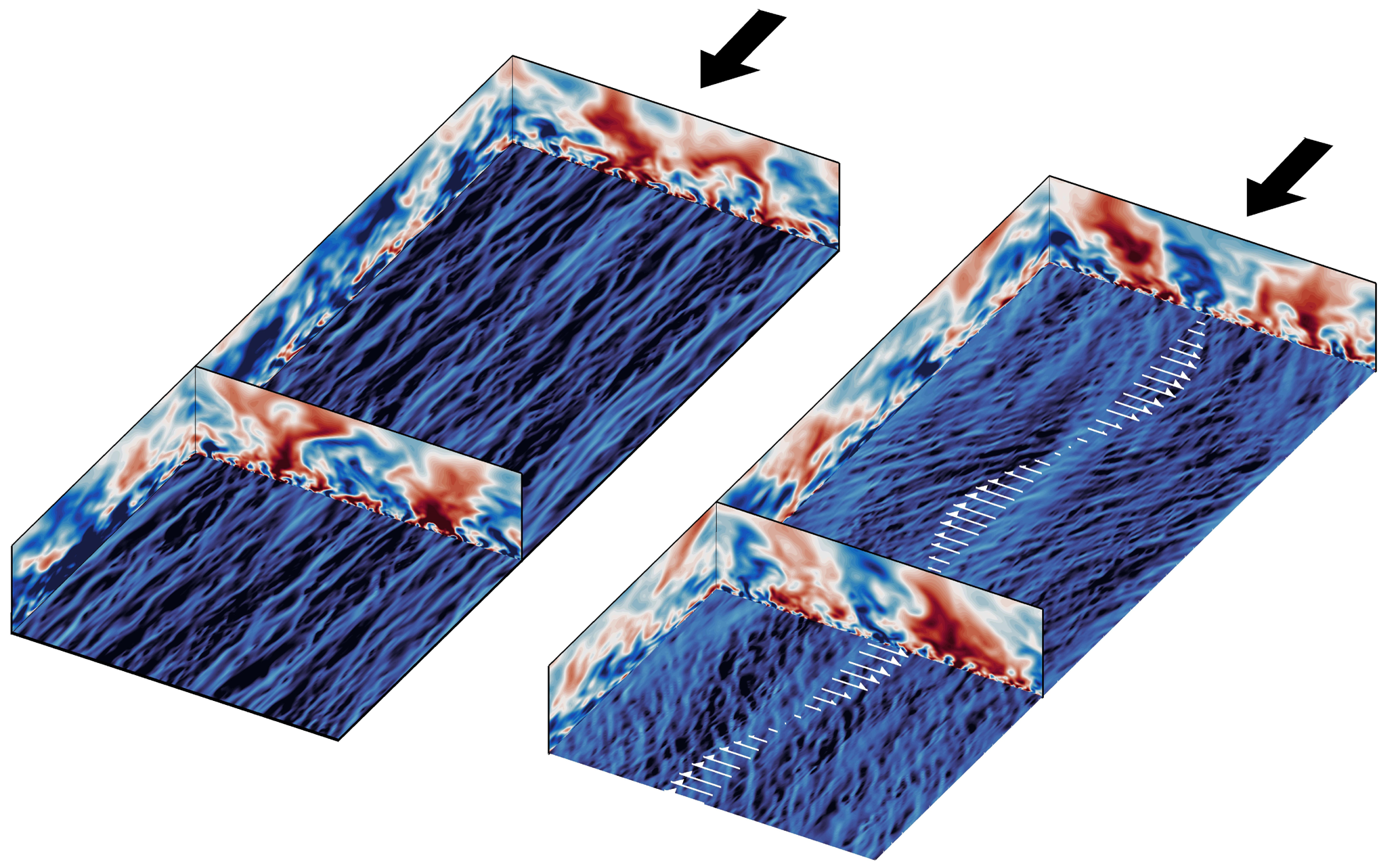
Various domain sizes for LES in a channel configuration: (a) medium  $2.0h \times 0.6h$, (b) large $4.0h \times 1.2h$ and (c) full $6.6h \times 3.2 h$. For each domain size, the instantaneous streamwise velocity ( $u$) field is visualised at about $15$ viscous units above the bottom wall. The grey-shaded zones indicate the wall heights up to which the flow is resolved for each domain size ( $y_{res} \simeq 0.4 L_z$, Chung et al. Reference Chung, Chan, MacDonald, Hutchins and Ooi2015).

Equations (2.1a,b) are solved using an LES extension of the DNS code by Chung, Monty & Ooi (Reference Chung, Monty and Ooi2014). We perform wall-resolved LES in a channel flow (figure 1) by applying periodic boundary conditions in the streamwise and spanwise directions. At the bottom wall we apply  $\hat {u}=\hat {v} = 0$ and $\hat {w}(x,z,t) = A\sin (\kappa _x x - \omega t)$, and at the top boundary we apply free-slip and impermeable conditions ( $\partial \hat {u}/\partial y = \partial \hat {w}/\partial y = \hat {v} = 0$). The present channel flow, with free-slip top boundary conditions and domain height $h$, is also called open channel flow (Yuan & Piomelli Reference Yuan and Piomelli2014; MacDonald et al. Reference MacDonald, Chung, Hutchins, Chan, Ooi and García-Mayoral2017; Endrikat et al. Reference Endrikat, Modesti, MacDonald, García-Mayoral, Hutchins and Chung2021b). This configuration is different to the open channel known in hydraulics, as a channel filled with water with the top wavy surface interacting with air (Chaudhry Reference Chaudhry2008; Yoshimura & Fujita Reference Yoshimura and Fujita2020). The present open channel configuration cannot be replicated experimentally. However, its flow physics and statistics up to the logarithmic region are very similar to the conventional channel flow with no-slip top boundary conditions and domain height $2h$ (also known as full channel flow). The advantage of open channel flow is its lower computational cost compared with the full channel flow. As a result, it is employed to study turbulent flows over complex surfaces (Yuan & Piomelli Reference Yuan and Piomelli2014; MacDonald et al. Reference MacDonald, Chung, Hutchins, Chan, Ooi and García-Mayoral2017; Rouhi, Chung & Hutchins Reference Rouhi, Chung and Hutchins2019; Endrikat et al. Reference Endrikat, Modesti, MacDonald, García-Mayoral, Hutchins and Chung2021b). Yao, Chen & Hussain (Reference Yao, Chen and Hussain2022) compare DNS of open channel flow with full channel flow up to $Re_\tau = 2000$. At $Re_\tau = 2000$, the mean velocity profiles between open channel flow and full channel flow yield identical diagnostic functions $y^+ \,{\rm d}U^+/{{\rm d}y}^+$ up to $y^+ \simeq 400$ (their figure 2). Furthermore, the turbulent stresses are similar between the two channel configurations (their figure 3). In figure 2(a) we obtain good agreement in the mean velocity profiles between our LES of open channel flow at $Re_\tau = 4000$ (black solid line) and DNS of full channel flow at $Re_\tau = 4200$ by Lozano-Durán & Jiménez (Reference Lozano-Durán and Jiménez2014) (filled squares), with only $1\,\%$ difference in $C_f$. Therefore, for our considered range of $Re_\tau \le 4000$ with the ISA pathway, we speculate marginal differences between open channel flow and full channel flow. Similarly, we speculate small differences between open channel flow and the boundary layer when we focus on the ISA pathway. This is supported by extensive comparisons of the channel flow with the boundary layer (Mathis et al. Reference Mathis, Monty, Hutchins and Marusic2009; Monty et al. Reference Monty, Hutchins, Ng, Marusic and Chong2009; Chin, Monty & Ooi Reference Chin, Monty and Ooi2014). The two configurations have identical mean velocity profiles up to the end of the logarithmic region (see figure 1a in Monty et al. Reference Monty, Hutchins, Ng, Marusic and Chong2009). Up to the fourth-order statistics are in agreement between the two configurations to a height of half the boundary layer thickness (half the channel height), e.g. see figure 3 in Mathis et al. (Reference Mathis, Monty, Hutchins and Marusic2009). However, differences appear in the outer region due to the differences in the large-scale motions. Nevertheless, in the ISA pathway these large-scale motions do not contribute to DR.
(a) Profiles of the mean velocity  $U^*$ for the LES of the actuated case at $Re_\tau = 4000, A^+ = 12, \kappa ^+_x = 0.02$ and $\omega ^+ = -0.05$ (blue solid line, blue dashed-dotted line), and LES of the non-actuated case at $Re_\tau = 4000$ (black solid line, black dashed-dotted line). The viscous-scaled quantities $U^*$ and $y^*$ are scaled by the actual values of $u_\tau$ for each case. The resolved portion of each LES profile $(y^* \lesssim 750)$ is shown with a solid line, and the unresolved portion $(y^* \gtrsim 750)$ is shown with a dashed-dotted line. The unresolved portion of each profile appears as a fictitious wake and is due to the medium-domain size (figure 1a). We reconstruct the unresolved portion using the composite profile for channel flow by Nagib & Chauhan (Reference Nagib and Chauhan2008) (the dashed lines for $y^* \gtrsim 750$). We compare the resolved (black solid line) and reconstructed (black dashed line) portions of the non-actuated LES with the DNS of Lozano-Durán & Jiménez (Reference Lozano-Durán and Jiménez2014) at $Re_\tau = 4200$ ( $\blacksquare$, red). (b) Difference between the actuated and non-actuated profiles $\Delta U^* = U^*_{act} - U^*_{non\text {-}act}$ (blue and black profiles in a) up to the maximum resolved height $y^*_{res} \simeq 750$. To reconstruct the actuated profile beyond $y^*_{res} \simeq 750$ using the composite profile suggested by Nagib & Chauhan (Reference Nagib and Chauhan2008), we set the log-law shift $\Delta B$ as the value of $\Delta U^*$ at $y^*_{res}$.

2.2. Simulation cases
Table 1 lists all the simulations completed for  $Re_\tau = 951$ and $Re_\tau = 4000$, where $Re_\tau \equiv u_{\tau _0} h/\nu$ represents the friction Reynolds number of the non-actuated case. At each $Re_\tau$, a parametric sweep of $7 \times 8$ combinations of streamwise wavenumber ( $\kappa ^+_x$) and oscillation frequency ( $\omega ^+$) is conducted over $0.00238 \le \kappa ^+_x \le 0.02$ and $-0.2 \le \omega ^+ \le +0.2$. The spanwise velocity amplitude is fixed at $A^+ = 12$. The seven non-zero values of $\omega ^+$ give the oscillation time periods $T_{osc}^+=126$, 63, 42 and 31 (all within the ISA pathway), and $\omega ^+=0$ corresponds to a time-invariant standing wave in the streamwise direction. In table 1, N/A denotes the specifications of the non-actuated simulation that serves as the reference case for calculating DR. For each actuated case, DR is computed by matching the bulk Reynolds number $Re_b = U_b h /\nu$ between the actuated and non-actuated cases and substituting the respective values of $C_f$ and $C_{f_0}$ into (1.2). We consider matched bulk Reynolds numbers $Re_b = 19\,700$ and $94\,450$, which correspond to $Re_\tau = 951$ and $4000$ for the non-actuated channel flow. Quadrio & Ricco (Reference Quadrio and Ricco2011) and Ricco et al. (Reference Ricco, Ottonelli, Hasegawa and Quadrio2012) compute $C_f$ and $C_{f_0}$ at matched $Re_\tau$ (instead of matched $Re_b$) by driving the actuated and non-actuated cases with a constant pressure gradient. Several differences exist between matching $Re_b$ (constant flow rate) and matching $Re_\tau$ (constant pressure gradient); see Quadrio & Ricco (Reference Quadrio and Ricco2011), Quadrio (Reference Quadrio2011) and Ricco et al. (Reference Ricco, Ottonelli, Hasegawa and Quadrio2012). With matched $Re_b$, $C_f$ and $C_{f_0}$ are obtained at different $Re_\tau$. However, for our considered parameter space, the maximum DR is about $30\,\%$, which leads to a maximum deviation of about $16\,\%$ in $Re_\tau$ between $C_f$ and $C_{f_0}$. Another source of difference between matched $Re_b$ and matched $Re_\tau$ is in the actuation amplitude $A$ (1.1). With constant $A^+ = 12$, $A^* = 12$ for the actuated cases with matched $Re_\tau$. However, with matched $Re_b$, $A^* > 12$ when ${\rm DR} > 0$, and vice versa. Nevertheless, DR weakly depends on $A^* \gtrsim 12$ (Quadrio et al. Reference Quadrio, Ricco and Viotti2009; Gatti & Quadrio Reference Gatti and Quadrio2016; Chandran et al. Reference Chandran, Zampiron, Rouhi, Fu, Wine, Holloway, Smits and Marusic2023). Overall, we speculate marginal differences in DR between matched $Re_b$ and matched $Re_\tau$ for our parameter space. According to Frohnapfel, Hasegawa & Quadrio (Reference Frohnapfel, Hasegawa and Quadrio2012), in internal flows, operation of a drag-reducing mechanism with matched $Re_b$ compared with the non-actuated case, saves the pumping energy but maintains the flow rate. On the other hand, operation with matched $Re_\tau$ maintains the pumping energy but increases the flow rate, hence reducing the time to transport fluid along the duct. Depending on the application, saving both energy and time could be important. Frohnapfel et al. (Reference Frohnapfel, Hasegawa and Quadrio2012) propose that operation of a drag-reducing mechanism with matched power input ( $\tau _w U_b = \mathrm {const.}$) leads to simultaneous saving of pumping energy (due to the reduction in $\tau _w$) and time (due to the increase in $U_b$).
Summary of the parameters of the computational runs. The top eight cases are conducted at  $Re_\tau = 951$ ( $Re_b = 19\,700$), and the bottom nine cases are conducted at $Re_\tau = 4000$ ( $Re_b = 94\,450$). The cases with N/A for $\kappa ^+_x$ and $\omega ^+$ correspond to the non-actuated reference cases. For all the actuated cases, $A^+ = 12$. Each row of the actuated cases consists of a set of cases with equal domain size, $Re_\tau$, $\kappa ^+_x$ and grid size, but $\omega ^+$ is different for each case (as listed in the fifth column). Those values of $\omega ^+$ with a $\pm$ sign indicate two separate simulations, one with a positive sign (downstream travelling wave) and one with a negative sign (upstream travelling wave). The first column indicates the domain size (see figure 1); at $Re_\tau = 951$ we use the full domain and at $Re_\tau = 4000$ we use the medium domain. The third column $y^+_{res}$ is the maximum resolved height by the simulation domain ( $\simeq 0.4 L^+_z$, Chung et al. Reference Chung, Chan, MacDonald, Hutchins and Ooi2015). The eighth row at $Re_\tau = 4000$ repeats some of the cases with $\kappa ^+_x = 0.007$ (the third row at $Re_\tau = 4000$), but with a finer grid resolution.

The grid resolutions were chosen based on extensive validation studies as presented in Appendices A and B. In these appendices we compare our LES results with DNS data of Gatti & Quadrio (Reference Gatti and Quadrio2016) at  $Re_\tau \approx 1000$, experimental data of Marusic et al. (Reference Marusic, Chandran, Rouhi, Fu, Wine, Holloway, Chung and Smits2021) at $Re_\tau = 6000$ and our self-generated DNS data at $Re_\tau = 590$. For DR and the mean velocity profile, we used the same viscous-scaled grid resolution at $Re_\tau = 951$ and $4000$, corresponding to the streamwise and spanwise grid sizes of $\varDelta ^+_x \times \varDelta ^+_z \simeq 21 \times 31$ (the first seven rows at each $Re_\tau$ in table 1). At this grid resolution, the difference in DR between the LES and DNS was found to be within $2\,\%$, and similarly good agreement was found for the mean velocity profile. However, for the Reynolds stresses and spectra at $Re_\tau = 4000$, we used a finer grid resolution with $\varDelta ^+_x \times \varDelta ^+_z \simeq 14 \times 21$ (the last two rows in table 1). Our nominal LES filter width $\varDelta ^+ = ( \varDelta ^+_x \varDelta ^+_y \varDelta ^+_z )^{1/3}$ is $7 \lesssim \varDelta ^+ \lesssim 34$ for the coarser grid and $5 \lesssim \varDelta ^+ \lesssim 22$ for the finer grid. However, given our anisotropic grid, we estimate our effective filter width from the two-dimensional energy spectrograms (figure 16e, f). Our maximum filter width is in the spanwise direction and is about $50$ and $35$ viscous units for the coarser and finer grids, respectively, equivalent to the cutoff wavenumbers $k^+_{\Delta _z} \simeq 0.12$ and $0.18$. These wavenumbers are $6$ and $9$ times larger than our maximum actuation wavenumber $\kappa ^+_x = 0.02$. We estimate our cutoff frequency from Taylor's frozen turbulence hypothesis (Taylor Reference Taylor1938). The most challenging zone in terms of resolution is the buffer region ( $y^+ \simeq 10$) with the smallest energetic eddies. If we take the convective speed of $10 u_{\tau _0}$ in this region, our cutoff frequencies are $\omega ^+_{\Delta _z}\simeq 1.2$ and $1.8$ for the coarser and finer grids, respectively, which are $6$ and $9$ times larger than our maximum actuation frequency $\omega ^+ = \pm 0.2$.
In terms of the domain size, the cases at  $Re_\tau = 951$ used a full domain with $L_x \times L_z \simeq 6.6 h \times 3.2 h$ (figure 1c), which is sufficiently large to resolve the first- and second-order statistics across the entire channel (Lozano-Durán & Jiménez Reference Lozano-Durán and Jiménez2014). However, at $Re_\tau = 4000$ each full-domain calculation is about $500$ times more expensive than that at $Re_\tau = 951$, and so the domain size was reduced to $L_x \times L_z \simeq 2.0h \times 0.6h$ (figure 1a). As a consequence, the flow is only resolved up to a fraction of the channel height $y^+_{res} \simeq 0.4 L^+_z$ (Chung et al. Reference Chung, Chan, MacDonald, Hutchins and Ooi2015), shown by the grey-shaded zones in figure 1. For a reduced-domain calculation, the user decides the resolved height $y^+_{res}$, with the constraint that it must fall somewhere in the logarithmic region. Then the domain size is obtained from the prescriptions of Chung et al. (Reference Chung, Chan, MacDonald, Hutchins and Ooi2015) and MacDonald et al. (Reference MacDonald, Chung, Hutchins, Chan, Ooi and García-Mayoral2017). For the travelling wave actuation (1.1), the prescriptions are $L^+_z \simeq 2.5 y^+_{res}, L^+_x \gtrsim \max (3L^+_z, 1000, \lambda ^+)$, where $\lambda$ is the travelling wavelength. MacDonald et al. (Reference MacDonald, Chung, Hutchins, Chan, Ooi and García-Mayoral2017, Reference MacDonald, Ooi, García-Mayoral, Hutchins and Chung2018) used the reduced-domain approach with $60 \lesssim y^+_{res} \lesssim 250$ for turbulent flows over roughness. Endrikat et al. (Reference Endrikat, Modesti, MacDonald, García-Mayoral, Hutchins and Chung2021b) used the same approach with $y^+_{res} \simeq 100$ for turbulent flows over riblets. Jiménez & Moin (Reference Jiménez and Moin1991) who used this approach for the first time resolved the flow up to $y^+_{res} \simeq 80$. They named this approach ‘minimal flow unit’. Here, with $L_x \times L_z \simeq 2.0h \times 0.6h$ (figure 1a) at $Re_\tau = 4000$, we resolve a substantial fraction of the inner layer up to $y^+_{res} \simeq 1000$. Therefore, we name our reduced domain the ‘medium domain’ to highlight its relatively larger size compared with the minimal flow unit. Gatti & Quadrio (Reference Gatti and Quadrio2016) also used the medium-domain size of $L_x \times L_z \simeq 1.4h \times 0.7h$ with $y^+_{res} \simeq 250$ to study the travelling wave (1.1). In Appendix C we assess the suitability of the medium-domain size (figure 1a) by comparing the results with those obtained using a larger domain size (figure 1b) for selected cases from table 1.
2.3. Calculation of the skin-friction coefficient
To compute DR (1.2), we need the skin-friction coefficient  $C_f \equiv 2\overline {\tau _w}/(\rho U^2_b) \equiv 2/{U^*_b}^2$ for both the actuated and non-actuated cases. Here, $U^*_b = \int _0^{h^*} U^* \,{{\rm d} y}^*/h^*$ is the viscous-scaled bulk velocity. For the cases at $Re_\tau = 951$ with the full-domain size, the $U^*$ profile is resolved across the whole channel and $U^*_b$ can be found directly. However, for the cases at $Re_\tau = 4000$ with the medium-domain size, the $U^*$ profile is resolved only up to $y^*_{res} \simeq 750\unicode{x2013}1000$. Two of these high-Reynolds-number profiles are shown in figure 2(a): the actuated case with $A^+=12$, $\kappa ^+_x = 0.02$ and $\omega ^+ = -0.05$ (blue lines), and the non-actuated case (black lines). The resolved portion of the LES profile below $y^*_{res}$ is shown with a solid line, and the unresolved portion above $y^*_{res}$ with a dashed-dotted line. We also overlay the DNS of the non-actuated full-domain channel flow at $Re_\tau = 4200$ by Lozano-Durán & Jiménez (Reference Lozano-Durán and Jiménez2014) (red squares). For the non-actuated LES, the resolved portion up to $y^*_{res} \simeq 1000$ (solid black line) accurately reproduces the non-actuated DNS. However, the unresolved portion beyond $y^*_{res}$ (black dashed-dotted line) departs from the non-actuated DNS due to the reduced-domain size.
This issue has been addressed previously by Chung et al. (Reference Chung, Chan, MacDonald, Hutchins and Ooi2015), MacDonald et al. (Reference MacDonald, Chung, Hutchins, Chan, Ooi and García-Mayoral2017), Endrikat et al. (Reference Endrikat, Modesti, García-Mayoral, Hutchins and Chung2021a) and Endrikat et al. (Reference Endrikat, Modesti, MacDonald, García-Mayoral, Hutchins and Chung2021b). For the accurate prediction of  $U^*_b$, hence $C_f$, it was found that the resolved height $y^*_{res}$ must fall inside the logarithmic region, and it needs to be larger than the extent of the disturbed flow due to the surface modification. If $y^*_{res}$ satisfies these criteria, the $U^*$ profile is resolved up to a portion of the log region, similar to the LES cases shown in figure 2(a). Beyond $y^*_{res}$, the unresolved portion of the log region and the outer region is assumed to be universal and so it can be reconstructed based on previous work. Here, we reconstruct the unresolved portions using the composite profile for the full-domain channel flow (Nagib & Chauhan Reference Nagib and Chauhan2008).
Figure 2(a) demonstrates that for the non-actuated case at  $Re_\tau =4000$, we obtain good agreement between the reconstructed profile for LES (dashed black line) and DNS. Therefore, to obtain $U^*_b$, we integrate the resolved $U^*$ profile up to $y^*_{res}$ and the reconstructed profile beyond $y^*_{res}$. We find that $C_{f_0}$ using this corrected $U^*_b$ is only $1\,\%$ different than the value obtained from DNS.
We follow the same approach to reconstruct the actuated  $U^*$ profile (dashed blue line in figure 2a). However, we need to add the log-law shift $\Delta B$ in the composite profile to make the resolved and reconstructed profiles continuous at $y^*_{res}$. We find $\Delta B$ by plotting the velocity difference between the actuated and non-actuated profiles $\Delta U^* = U^*_{act} - U^*_{non{\text {-}}actuated}$ (figure 2b). As seen in figure 2(b), $\Delta U^*$ reaches almost a plateau beyond $y^* \simeq 100$. We set $\Delta B$ as the value of $\Delta U^*$ at $y^*_{res} \simeq 750$. Note that since the actuated $u_\tau$ is smaller than the non-actuated $u_{\tau _o}$, $y^*_{res}$ for the actuated case is about $750$ but, for the non-actuated case, is about $1000$. We calculate $U^*_b$ for the actuated case by integrating the resolved portion of the profile up to $y^*_{res}$ (solid blue line) and the reconstructed portion beyond $y^*_{res}$ (dashed blue line).
Another way of calculating  $U^*_b$ (hence, $C_f$) from the reduced domain is to integrate the composite profile from $y=0$ to $h$ (e.g. see 4.2 in MacDonald, Hutchins & Chung Reference MacDonald, Hutchins and Chung2019), which assumes that the viscous sublayer and buffer layer make a negligible contribution to $U^*_b$. We believe that our present approach is more accurate as it considers the complex variation of $U^*$ in the viscous sublayer and buffer layer. We only use the composite profile in the log region and beyond.
3. Results
3.1. Drag reduction map as a function of frequency and wavelength
Figure 3(a,b) display the maps of  ${\rm DR}(\omega ^+,\kappa ^+_x)$ at $Re_\tau = 951$ and $4000$ from the computations listed in table 1. At each $Re_\tau$, we have $56$ DR data points. To generate the maps, we perform bilinear interpolation of our DR data points onto a uniform $20 \times 20$ grid over the parameter space $0 \le \kappa ^+_x \le 0.02$ and $-0.2 \le \omega ^+ \le +0.2$. At $Re_\tau = 951$, the maximum DR of $35.4\,\%$ at $(\omega ^+,\kappa ^+_x) = (0.05,0.021)$ is in close agreement with the DNS of Gatti & Quadrio (Reference Gatti and Quadrio2016) at $Re_\tau \simeq 950$, where the maximum DR was found to be $38.8\,\%$ at $(\omega ^+,\kappa ^+_x) = (0.05, 0.0195)$. At $Re_\tau = 4000$, the maximum DR decreases to $27.5\,\%$ at the same actuation parameters $(\omega ^+,\kappa ^+_x) = (0.05,0.021)$. At each Reynolds number, DR changes more drastically by changing $\omega ^+$ than by changing $\kappa ^+_x$.
(a,b) Maps of DR for  $A^+ =12$ at (a) $Re_\tau = 951$ and (b) $Re_\tau = 4000$. The local maximum DR (blue dashed-dotted line) and the local minimum DR (black dashed line) for $\kappa ^+_x > 0$ are indicated for clarity. We label the region on the left-hand side of the blue dashed-dotted line with I, between the blue dashed-dotted line and the black dashed line with II and the right-hand side of the black dashed line with III. (c) Map of the difference in DR between $Re_\tau = 4000$ and $Re_\tau = 951$. (d) Map of the difference in DR between $Re_\tau = 4000$ and GQ's prediction (Gatti & Quadrio Reference Gatti and Quadrio2016) at the same Reynolds number. In plots (a–d) the contour fields and the contour lines show the same quantity. For plots (a,b), the contour lines grow from $-20\,\%$ to $40\,\%$ and, for (c,d), the contour lines grow from $-7\,\%$ to $+7\,\%$.

When  $\kappa ^+_x = 0$, there is no travelling wave (plane wall oscillation), and the variation of the DR is symmetric between $\omega ^+ <0$ and $\omega ^+ > 0$. In this case, two equal local maxima (at $\omega ^+ \simeq \pm 0.05$) and a local minimum (at $\omega = 0$) emerge. When $\kappa ^+_x >0$, a travelling wave is generated, and the variation of DR is asymmetric between $\omega ^+ < 0$ and $\omega ^+ > 0$. In this case, at each $\kappa ^+_x$ only one local maximum (blue dashed-dotted curve in figure 3) and one local minimum (black dashed curve in figure 3) appear in the DR. These observations are in agreement with Quadrio et al. (Reference Quadrio, Ricco and Viotti2009) and Gatti & Quadrio (Reference Gatti and Quadrio2016). Overall, within our parameter space, the map of DR consists of three distinct regions. Region I to the left of the local maximum DR (blue dashed-dotted curve) where $\omega ^+ \lesssim 0$ (upstream travelling wave); in this region ${\rm DR}> 0$. Region II represents the crossover from the local maximum to the local minimum DR (between the blue dashed-dotted curve and the black dashed curve). For $\kappa ^+_x \lesssim 0.007$, the local minimum DR is positive, however, for $\kappa ^+_x \gtrsim 0.007$, the local minimum DR becomes negative (hence, a drag increase). Increase in $\kappa ^+_x$ beyond $0.007$ leads to a larger drag increase area, and the local minimum DR becomes more negative; Quadrio et al. (Reference Quadrio, Ricco and Viotti2009) and Gatti & Quadrio (Reference Gatti and Quadrio2016) observe similar trends. Quadrio et al. (Reference Quadrio, Ricco and Viotti2009) find that the local minimum DR follows the line $\omega ^+/\kappa ^+_x \simeq 10$. In other words, a maximum drag increase occurs when the travelling wave speed is about $10u_{\tau _0}$, which is nearly the same as the convective speed of the near-wall flow structures. Similarly, in figure 3(a,b) the black dashed curve that marks the local minimum DR follows $\omega ^+/\kappa ^+_x \simeq 10$. Region III covers the right of the local minimum DR (black dashed curve) where $\omega ^+ > 0$ (downstream travelling wave); in this region an increase in $\omega ^+$ increases the DR.
In figure 3(c) we display the difference in DR as the Reynolds number changes from 4000 to 951. For most of the  $(\omega ^+, \kappa ^+_x)$ space, DR is lower at the higher Reynolds number. Only within the range $0.005 \lesssim \kappa ^+_x \lesssim 0.020, +0.1 \lesssim \omega ^+ \lesssim +0.2$ do we observe the opposite trend. This region coincides with the drag-increasing range ( ${\rm DR} < 0$) with $\omega ^+ > 0$. This observation is consistent with GQ's model (1.5), where ${\rm DR} <0$ (hence, $\Delta B < 0$) predicts an increase in DR as the Reynolds number increases. To make these comparisons more quantitative, in figure 3(d) we show the difference in DR between our results and GQ's model at $Re_\tau = 4000$. To predict DR, the model (1.5) requires $C_{f_0}$ and the value of the log-law shift $\Delta B$ for each set of actuation parameters $(A^+, \kappa ^+_x, \omega ^+)$. For $C_{f_0}$, we use Dean's power-law correlation (Dean Reference Dean1978) that agrees well with the DNS data given by MacDonald et al. (Reference MacDonald, Hutchins and Chung2019). We can obtain $\Delta B$ from a low-Reynolds-number simulation for the same set of $(A^+, \kappa ^+_x, \omega ^+)$ because $\Delta B$ is assumed to be Reynolds number independent. Therefore, we use our results at $Re_\tau = 951$, where for each $(\omega ^+, \kappa ^+_x)$, we find $\Delta B$ from the velocity difference $\Delta U^*$ at $y^* = 200$ (similar to figure 2b). We choose $y^* = 200$ as it is far enough from the wall to fall into the log region, but not too far to fall into the wake region ( $y/h \gtrsim 0.3$ according to Pope Reference Pope2000). By having $\Delta B$ at each $(\omega ^+, \kappa ^+_x)$ and having $C_{f_0}$ at $Re_\tau = 4000$, we can reconstruct the DR map based on GQ's model.
Figure 3(d) shows the overall good performance of GQ's model for this range of Reynolds numbers. In region I the difference in DR between LES and GQ's model is less than  $2\,\%$, i.e. $|{\rm DR}\%_{LES,Re_\tau = 4000} - {\rm DR}\%_{GQ,Re_\tau = 4000}| \lesssim 2\,\%$. This is a very good agreement considering that DR varies between $15\,\%$ and $28\,\%$ in region I. In regions II and III we observe some slight differences in DR between LES and GQ's model, especially in region II in the drag-increasing range. In this range, the difference in DR between LES and GQ's model reaches $4\,\%$, which is the same order as DR (see figure 3b). In region III, for $\omega ^+ \gtrsim +0.1$ again, we observe good agreement between LES and GQ's model (less than $2\,\%$ difference). In the following sections we investigate the reasons behind the different performance of GQ's model in regions I, II and III related to the changes in the Stokes layer dynamics and the near-wall turbulence in each of these regions.
3.2. Mean velocity profiles
To obtain an overall picture of the mean velocity behaviour in regions I, II and III (see figure 4), we consider the seven runs conducted at  $Re_\tau = 4000, A^+ = 12$ and $\kappa ^+_x = 0.007$ for $\omega ^+$ ranging from $-0.2$ to $+0.2$. In figure 4(a) we identify the selected values of $\omega ^+$ (filled squares) on the DR map along with the local maximum DR (blue dashed-dotted line) and the local minimum DR (black dashed line). The corresponding velocity profiles are shown in figure 4(b,c) for $\omega ^+ \le 0$ (upstream travelling waves) up to the local maximum DR (region I) and $\omega ^+ \ge 0$ (downstream travelling waves) beyond the local maximum DR (regions II, III), respectively.
Variation of DR and the mean velocity profiles  $U^*$ at $Re_\tau = 4000$, $A^+ = 12$, $\kappa ^+_x = 0.007$ and $-0.2 \le \omega ^+ \le +0.2$. (a) Variation of DR with $\omega ^+$; the inset shows the location of the data points on the DR map. The blue dashed-dotted line and the black dashed line are the local maximum and minimum DR.(b,c) Variation of the $U^*$ profiles with $\omega ^+$ for (b) upstream travelling wave ( $\omega ^+ \le 0$) and (c) downstream travelling wave ( $\omega ^+ \ge 0$); the profile (— $\square$—) corresponds to the non-actuated case and the profiles with no symbol correspond to the actuated cases. For each profile, the solid line is the resolved portion and the dashed line is the reconstructed portion following Nagib & Chauhan (Reference Nagib and Chauhan2008). For each case, the colour of its $U^*$ profile in (b,c) is consistent with the colour of its DR data point in (a). In (b,c) the inset plots the same profiles in terms of $U^*/y^*$ vs $y^*$. (d,e) Diagnostic function $y^* \,{\rm d}U^*/{{\rm d} y}^*$ for the profiles in (b,c); the inset shows the velocity difference $\Delta U^* = U^*_{act} - U^*_{non{\text {-}}act}$ between each actuated profile $U^*_{act}$ and the non-actuated profile $U^*_{non{\text {-}}act}$.

When  $\omega ^+ \le 0$, the log region of the actuated profiles is shortened and shifted above the non-actuated counterpart (figure 4b), corresponding to a positive DR. The shortening of the log region is due to the thickening of the viscous sublayer. We show the viscous sublayer thickening in the inset of figure 4(b), in that the actuated profiles of $U^*/y^*$ are closer to unity for a greater wall distance compared with their non-actuated counterpart. We show the shortening of the log region in figure 4(d) by plotting the diagnostic function $y^* \,{\rm d}U^*/{{\rm d}y}^*$. The log region appears as a plateau with the value of $\kappa ^{-1} \simeq 2.5$. For the non-actuated case, the plateau appears for $100 \lesssim y^* \lesssim 600$. This range is consistent with the DNS of channel flow by Lozano-Durán & Jiménez (Reference Lozano-Durán and Jiménez2014) and Lee & Moser (Reference Lee and Moser2015) at $Re_\tau = 4200$ and $5200$, respectively (see figure 3a in Lee & Moser Reference Lee and Moser2015). For the actuated cases, the plateau is narrowed further (i.e. log region is shortened) as DR increases. We quantify the shift in the log region by plotting $\Delta U^*$ (inset of figure 4d). The magnitude of the shift increases as DR increases. These observations are also reported in the previous turbulent DR studies, including turbulent flow with the spanwise wall oscillation (Di Cicca et al. Reference Di Cicca, Iuso, Spazzini and Onorato2002; Touber & Leschziner Reference Touber and Leschziner2012; Hurst et al. Reference Hurst, Yang and Chung2014), turbulent flow with the streamwise travelling wave (Hurst et al. Reference Hurst, Yang and Chung2014; Gatti & Quadrio Reference Gatti and Quadrio2016), turbulent flow of a polymer solution (Ptasinski et al. Reference Ptasinski, Boersma, Nieuwstadt, Hulsen, Van den Brule and Hunt2003; White & Mungal Reference White and Mungal2008) and turbulent flow over piezoelectrically excited travelling waves (Musgrave & Tarazaga Reference Musgrave and Tarazaga2019). Gatti & Quadrio (Reference Gatti and Quadrio2016) derived their predictive model (1.5) based on similar observations of the velocity profiles in region I, and as a result, GQ's prediction works well in this region (figure 3d). The behaviour of the profiles in region I is consistent with the ISA pathway, where only the inner-scale eddies up to the buffer region are actuated.
In region II we observe a sudden drop in DR as  $\omega ^+$ changes from 0 to $+0.1$ (figure 4a), with a corresponding decrease in the logarithmic shift (figure 4c). A distinct feature of region II is the high level of distortion in the $U^*$ profile, which is particularly severe at $\omega ^+ = +0.05$. For this case, the diagnostic function tends towards the plateau $\kappa ^{-1}$, but does not reach it. Similarly, $\Delta U^*$ for this case approaches a plateau of $1.7$ by the resolved height $y^*_{res} \simeq 750$, but does not reach it (inset in figure 4e). This is our most challenging case for computing DR using our approach in § 2.3 (figure 2). For accurate calculation of the DR, $\Delta U^*$ needs to reach a plateau by the resolved height $y^*_{res} \simeq 750$, i.e. the resolved height must fall into the logarithmic region. In Appendix C we deliberately consider this challenging case for a domain size study. We double the domain length and width compared with the medium domain (figure 1b), extending the resolved height to $y^*_{res} \simeq 1500$. The difference in DR is $1.4\,\%$ between the medium domain and the large domain (table 4). Furthermore, the large domain reinforces the approach of $\Delta U^*$ to a plateau of $1.7$ (the inset in figure 18b). To our knowledge, such significant levels of distortion in the $U^*$ profile have not been seen before in previous studies of flows over drag-reducing or drag-increasing surfaces. For example, in rough wall turbulent flows $\Delta U^*$ is almost constant for $y^* \gtrsim 30$ (e.g. figure 6 in Chan et al. Reference Chan, MacDonald, Chung, Hutchins and Ooi2015 or figure 3 in MacDonald et al. Reference MacDonald, Chung, Hutchins, Chan, Ooi and García-Mayoral2017), while in turbulent flows over riblets $\Delta U^*$ is almost constant for $y^* \gtrsim 100$ (e.g. figure 2 in Endrikat et al. Reference Endrikat, Modesti, MacDonald, García-Mayoral, Hutchins and Chung2021b). In §§ 3.4 and 3.5 we discuss the physics behind the highly distorted mean velocity profiles (figure 4c,e).
Summary of the LES cases for the domain size study. For all cases,  $A^+ = 12$. We consider three cases with $(\kappa ^+_x, \omega ^+) = (0.021, -0.1), (0.021, +0.1), (0.007, +0.05)$. For each case, we perform a medium-domain simulation (figure 1a, $L_x \times L_z \simeq 2.0h \times 0.6 h, y^+_{res} \simeq 1000$), and a large-domain simulation (figure 1b, $L_x \times L_z \simeq 4.0h \times 1.2 h, y^+_{res}\simeq 2000$).

In region III, when  $\omega ^+$ increases to $+0.2$ (figure 4c), DR increases to $13\,\%$ and the $U^*$ profile behaves similarly to that seen in region I. A well-defined logarithmic shift appears beyond $y^* \simeq 100$ with viscous sublayer thickening.
3.3. Turbulence statistics
We now assess the behaviour of the Reynolds stress distributions at  $Re_\tau =4000$ (figure 5a–d) and the turbulent kinetic energy production $P = -\langle u' v' \rangle _{xzt}\, {\rm d}U/{{\rm d} y}$ (figure 5e, f), where $\langle \cdots \rangle _{xzt}$ denotes averaging over the $xz$ plane and time. We highlight four cases from figure 4 ( $A^+ = 12, \ \kappa ^+_x = 0.007$), where we vary $\omega ^+$ from $-0.05$ to $+0.20$. As indicated earlier, we employ a finer grid resolution for these cases to properly resolve the Reynolds stresses (see Appendix B). We plot the profiles scaled by the non-actuated $u_{\tau _0}$ (dashed-dotted lines, figure 5a,c) and by the actuated $u_\tau$ (solid lines, figure 5b,d). Scaling by $u_{\tau _0}$ is comparable to scaling by the bulk velocity $U_b$ (Gatti & Quadrio Reference Gatti and Quadrio2016) because the bulk velocity $U_b$ is the same between the actuated and non-actuated cases. Any difference between the outer-scaled actuated and non-actuated profiles reflects the overall response of turbulence to the wall oscillation (1.1).
Profiles of Reynolds stresses and turbulence production for four cases from figure 4 at  $Re_\tau = 4000, A^+ = 12, \kappa ^+_x = 0.007$ and $\omega ^+ = -0.05, 0, +0.05, +0.20$. The insets in (a,b) indicate the considered values of $\omega ^+$ and their DR values. Line and symbol colours are consistent with figure 4. In each panel only the resolved portion of the profiles are shown ( $y^+ \lesssim 1000, y^* \lesssim 700$). The black lines with symbols correspond to the non-actuated case. (a,c,e) Plot of the actuated profiles (dashed-dotted lines) scaled by the non-actuated $u_{\tau _0}$ (superscripted with $+$); (b,d, f) plot of the actuated profiles (solid lines) scaled by the actuated $u_\tau$ (superscripted with $*$). (a–d) Reynolds stress profiles for (a,b) the streamwise velocity $\langle u'^2 \rangle _{xzt}$ and (c,d) the spanwise velocity $\langle w'^2 \rangle _{xzt}$. (e, f) Premultiplied production of turbulent kinetic energy.

Scaling by the non-actuated  $u_{\tau _0}$ (‘ $+$’ superscript), as in figure 5(a,c,e), indicates that the wall oscillation attenuates the $\langle u'^2 \rangle ^+_{xzt}$ levels up to the resolved height $y^+_{res} \simeq 1000$. The cases with the highest DR ( $\omega ^+ = -0.05, 0$ in figure 5a) show the highest level of attenuation in their $\langle u'^2 \rangle ^+_{xzt}$. Additionally, for these cases, the inner peak of $\langle u'^2 \rangle ^+_{xzt}$ is farther from the wall. Consistently, the viscous sublayer is thickened and the buffer layer is shifted away from the wall (figure 4b). In contrast to the behaviour of $\langle u'^2 \rangle ^+_{xzt}$, the $\langle w'^2 \rangle ^+_{xzt}$ profiles are amplified near the wall. According to Quadrio & Ricco (Reference Quadrio and Ricco2011) and Touber & Leschziner (Reference Touber and Leschziner2012), this amplification is due to the Stokes layer that forms as a result of the spanwise wall motion. The premultiplied turbulent kinetic energy production $y^+ P^+$ (figure 5e) also displays the attenuation of turbulence that accompanies increasing DR. All these trends are similar to previous studies on spanwise wall oscillation at lower Reynolds numbers (Quadrio & Ricco Reference Quadrio and Ricco2011; Touber & Leschziner Reference Touber and Leschziner2012).
Scaling by the actuated  $u_\tau$ (‘ $*$’ superscript) is equivalent to inner scaling, which highlights the extent up to which the actuated profiles depart from the non-actuated profile. For $\langle u'^2 \rangle ^*_{xzt}$ and $\langle w'^2 \rangle ^*_{xzt}$ (figure 5b,d), the actuated cases agree with the non-actuated case at distances far from the wall, but near the wall the actuated $\langle u'^2 \rangle ^*_{xzt}$ levels are attenuated, while the $\langle w'^2 \rangle ^*_{xzt}$ levels are amplified. For $\omega ^+ = +0.05$ (in region II), the point where the actuated profiles begin to depart from the non-actuated counterpart occurs at $y^* \simeq 100$, considerably farther than for the other cases $(y^* \lesssim 30)$. The same case yields the strongest level of near-wall amplification for $\langle w'^2 \rangle ^*_{xzt}$ (the red profile in figure 5c,d) and the highest level of distortion in mean velocity (red profile in figure 4c,e).
Regardless of the scaling used, as  $\langle w'^2 \rangle _{xzt}$ is amplified near the wall, $\langle u'^2 \rangle _{xzt}$ is attenuated, the viscous sublayer is thickened and DR is increased. This trend occurs in regions I ( $\omega ^+ = -0.05, 0$) and III ( $\omega ^+ = +0.2$). In region II ( $\omega ^+ = +0.05$), however, there is an excessive amplification of $\langle w'^2 \rangle _{xzt}$ near the wall, a thinning of the viscous sublayer and a drop in DR.
3.4. Stokes layer: an important source of ISA
As indicated earlier, the near-wall amplification of  $\langle w'^2 \rangle _{xzt}$ is related to the growth of the Stokes layer. We now apply triple decomposition to more precisely uncover how the strength of the Stokes layer modifies the near-wall turbulence, which in turn affects the wall drag. We primarily consider $u_\tau$ scaling, as we are interested in the level of departure from the non-actuated behaviour. In Part 2 we mostly use $u_{\tau _0}$ scaling, as we are interested in studying the overall response of turbulence to the wall actuation. Nevertheless, the conclusions from Parts 1 and 2 are valid regardless of the scaling.
Because the flow is subjected to a harmonic forcing (1.1), the instantaneous flow can be triply decomposed similar to Touber & Leschziner (Reference Touber and Leschziner2012), as in
 $$\begin{gather} f(x,y,z,t) = \left\langle f \right\rangle_{xzt}(y) + \underbrace{\tilde{f}(x,y,t) + f''(x,y,z,t)}_{f'(x,y,z,t)}, \end{gather}$$
 $$\begin{gather}\tilde{f}(x,y,t) = \frac{1}{N}\sum_{n=0}^{N-1}\left\langle f \right\rangle_z (x,y,t+nT_{osc}) - \left\langle f \right\rangle_{xzt}(y), \end{gather}$$
 $$\begin{gather}\left\langle f'^2 \right\rangle_{xzt} = \left\langle \tilde{f}^2 \right\rangle_{xt} + \left\langle f''^2 \right\rangle_{xzt}, \end{gather}$$
where  $f$ indicates the quantity of interest, i.e. $u,v$ or $w$. In (3.1a), the total fluctuation $f'$ is decomposed into the harmonic contribution $\tilde {f}$ and the stochastic (turbulent) contribution $f''$. The harmonic contribution $\tilde {f}$ is obtained by phase averaging the spanwise averaged field $\langle f \rangle _z$ in time over the number of periods $N$, and then subtracting the mean vertical profile $\langle f \rangle _{xzt}$. Accordingly, the total Reynolds stress $\langle f'^2 \rangle _{xzt}$ is decomposed into its harmonic component $\langle \tilde {f}^2\rangle _{xt}$ associated with the Stokes layer dynamics and its turbulent (stochastic) component $\langle f''^2\rangle _{xzt}$ (3.1c).
In figure 6 we plot these two components for the cases given in figures 4 and 5 ( $A^+ = 12, \kappa ^+_x = 0.007$, $Re_\tau =4000$). For reference, figure 6(a,b) shows the considered $U^*$ profiles (as in figure 4b,c). Figure 6(c,d) displays $\langle u''^2\rangle ^*_{xzt}$, the stochastic component of the streamwise Reynolds stress. By comparing figure 5(b) with figure 6(c,d), we see that $\langle u'^2\rangle ^*_{xzt} \simeq \langle u''^2\rangle ^*_{xzt}$, indicating that the harmonic (Stokes layer) component makes a negligible contribution. For the spanwise velocity, however, the harmonic component $\langle \tilde {w}^2\rangle ^*_{xt}$ contributes significantly to the total spanwise Reynolds stress $\langle w'^2\rangle ^*_{xzt}$ close to the wall (see figure 6e, f). At $y^* \sim {O}(1)$, the harmonic component is about three orders of magnitude larger than the turbulent component, while at $y^* \sim {O}(10)$ they have comparable magnitudes. Figure 6(e, f) indicates that the rate of decay in $\langle \tilde {w}^2 \rangle ^*_{xt}$, hence the protrusion of the Stokes layer, strongly depends on $\omega ^+$. Furthermore, the level of distortion in the $U^*$ profiles (figure 6a,b) strongly depends on the rate of decay in $\langle \tilde {w}^2 \rangle ^*_{xt}$. Interestingly, in region II (figure 6f) the decay rate in $\langle \tilde {w}^2 \rangle ^*_{xt}$ is noticeably slower compared with regions I and III, implying the presence of a more protrusive Stokes layer. Accordingly, the $U^*$ profile in region II is distorted to the highest level. The turbulent stress profiles are also shown in figure 8, where they are accompanied by the turbulent kinetic energy profiles $\langle \mathcal {K} \rangle _{xzt}$, which follow the same trends.
Profiles of velocity statistics at  $Re_\tau =4000$ for given cases as in figures 4 and 5 ( $A^+ = 12, \kappa ^+_x = 0.007$). Line legends are consistent with figures 4 and 5. In each panel only the resolved portion of the profiles are shown corresponding to $y^* \le 1000$. Plots (a,c,e) correspond to $\omega ^+ \le 0$, and plots (b,d, f) correspond to $\omega ^+ > 0$. (a,b) The $U^*$ profiles; the insets indicate the value of $\omega ^+$ and its DR for each profile. In (c–f) the Reynolds stress profiles are presented in terms of the turbulent component (solid lines) and the harmonic component (dashed lines) following ((3.1a), (3.1b)). (c,d) Turbulent component of the streamwise velocity $\langle u''^2 \rangle ^*_{xzt}$. (e, f) Turbulent component $\langle w''^2 \rangle ^*_{xzt}$ and harmonic component $\langle \tilde {w}^2 \rangle ^*_{xt}$ for the spanwise velocity. On each actuated profile, the cross symbol (+) marks the Stokes layer thickness $\delta ^*_S$, and the bullet symbol ( $\bullet$) marks the protrusion height $\ell ^*_{0.01}$ due to the Stokes layer.

To quantify the protrusion of the Stokes layer (figure 6e, f), we calculate two length scales from the spanwise Reynolds stress profiles. The first is the laminar Stokes layer thickness  $\delta ^*_S$ that is featured in Stokes’ second problem (Batchelor Reference Batchelor2000). Following Quadrio & Ricco (Reference Quadrio and Ricco2011), we define $\delta ^*_S$ as the height $y^*$ where the amplitude of $\tilde {w}$ decays to $A {\rm e}^{-1}$ (i.e. where $\langle \tilde {w}^2 \rangle ^*_{xt} = {\tfrac {1}{2}}{A^*}^2 {\rm e}^{-2}$). In figure 6 we mark $\delta ^*_S$ on each profile with a cross symbol. The second length scale $\ell ^*_{0.01}$ is new, and it is defined as the height where $\langle \tilde {w}^2 \rangle ^*_{xt} = 0.01$. Our choice for the threshold of $\langle \tilde {w}^2 \rangle ^*_{xt} = 0.01$ is based on the observation that $\langle w''^2 \rangle ^*_{xzt} \sim {O}(1)$ in the buffer and log regions (also reported by Lee & Moser Reference Lee and Moser2015; Baidya et al. Reference Baidya, Philip, Hutchins, Monty and Marusic2021). In other words, we define $\ell ^*_{0.01}$ as the height where the Stokes layer stress $\langle \tilde {w}^2 \rangle ^*_{xt}$ drops to about $1\,\%$ of the spanwise turbulent stress $\langle w''^2 \rangle ^*_{xzt}$. In figure 6 we mark $\ell ^*_{0.01}$ on each profile with a bullet symbol.
The key difference between  $\delta ^*_S$ and $\ell ^*_{0.01}$ is that we mark $\delta ^*_S$ where the Stokes layer stress $\langle \tilde {w}^2 \rangle ^*_{xt}$ is a small fraction of its maximum value at the wall ${A^*}^2/2$. Thus, we ignore the background turbulence in this definition. However, we mark $\ell ^*_{0.01}$ where the Stokes layer stress $\langle \tilde {w}^2 \rangle ^*_{xt}$ is a small fraction of the turbulent stress $\langle w''^2 \rangle ^*_{xzt}$, hence considering the background turbulence in this definition. In figure 6(c–f), $\ell ^*_{0.01}$ coincides well with the distance where the actuated $\langle u''^2 \rangle ^*_{xzt}$ and $\langle w''^2 \rangle ^*_{xzt}$ profiles depart from the non-actuated counterpart. However, $\delta ^*_S$ underestimates the actual protrusion by the Stokes layer due to its ignorance of the background turbulence. For instance, for the case with $\omega ^+ = 0$ at $y^* = \delta ^*_S$ (black cross symbol in figure 6e), $\langle \tilde {w}^2 \rangle ^*_{xt} \simeq 8 \langle w''^2 \rangle ^*_{xzt}$, i.e. the Stokes layer is $8$ times stronger than the background turbulence. However, at $y^* = \ell ^*_{0.01}$ (black bullet symbol), $\langle \tilde {w}^2 \rangle ^*_{xt} \simeq 0.01 \langle w''^2 \rangle ^*_{xzt}$, i.e. the Stokes layer is $100$ times weaker than the background turbulence. We propose, therefore, that $\ell ^*_{0.01}$ is a more suitable measure for reflecting the entire penetration of the Stokes layer into the turbulent field.
In regions I and III, the level of protrusion by the Stokes layer  $\ell ^*_{0.01}$, as well as the departure height in the $\langle u''^2 \rangle ^*_{xzt}$ and $\langle w''^2 \rangle ^*_{xzt}$ profiles, stay below $20 - 30$ viscous units. As a result, the mean velocity profiles in regions I and III (figure 6a,b) yield a well-defined logarithmic shift beyond $y^* \simeq 100$ with viscous sublayer thickening. However, in region II there is a large increase in $\ell ^*_{0.01}$ and the departure in the $\langle u''^2 \rangle ^*_{xzt}$ and $\langle w''^2 \rangle ^*_{xzt}$ profiles also starts at a larger distance from the wall. For example, for $\omega ^+ = +0.05$ in region II (figure 6d, f), $\ell ^*_{0.01} \simeq 80$, which also closely marks the point where the actuated $\langle u''^2 \rangle ^*_{xzt}$ and $\langle w''^2 \rangle ^*_{xzt}$ profiles depart from their non-actuated counterpart. As a result, the mean velocity profile for $\omega ^+ = +0.05$ in region II (figure 6b) is highly distorted up to $y^* \simeq 200\unicode{x2013}300$.
Furthermore, we can draw a connection between the protrusion height  $\ell ^*_{0.01}$ and the level of DR. In figure 7(a,b) we overlay the map of $\ell ^*_{0.01}$ onto the maps of DR and $\delta ^*_S$. In region I (left-hand side of the blue dashed-dotted line), $\ell ^*_{0.01} \lesssim 30$ and $\delta ^*_S \lesssim 7$. In this region, an increase in $\ell ^*_{0.01}$ and $\delta ^*_S$ leads to an increase in DR. For upstream travelling waves ( $\omega ^+ < 0$), therefore, the growing protrusion of the Stokes layer has a favourable effect on DR. In contrast, in region II (between the blue dashed-dotted line and the black dashed line) DR drops by increasing $\ell ^*_{0.01}$ and $\delta ^*_S$. Another difference between regions I and II is in the relation between $\ell ^*_{0.01}$ and $\delta ^*_S$. In region I, $\ell ^*_{0.01}$ and $\delta ^*_S$ are proportional to each other with $\ell ^*_{0.01}\approx 4\delta ^*_S$. However, in region II this proportional relation is broken and $\ell ^*_{0.01}$ can reach as high as $8\delta ^*_S$. At each $\kappa ^+_x$, the maximum DR (the blue dashed-dotted line) coincides with the optimal range $20 \lesssim \ell ^*_{0.01} \lesssim 30$ $(5 \lesssim \delta ^*_S \lesssim 7)$. In figure 7(c) we plot DR vs $\ell ^*_{0.01}$ for our simulation cases in regions I and II. Also, following Quadrio & Ricco (Reference Quadrio and Ricco2011) (their figure 9), we plot DR vs $\delta ^*_S$ for the same cases (figure 7d). These plots confirm that the maximum DR coincides with $20 \lesssim \ell ^*_{0.01} \lesssim 30$ and $5 \lesssim \delta ^*_S \lesssim 7$ (shaded in grey). Furthermore, for $\ell ^*_{0.01} \lesssim 20$ ( $\delta ^*_S \lesssim 5$), $\ell ^*_{0.01} \simeq 4 \delta ^*_S$ and DR increases linearly with $\ell ^*_{0.01}$ and $\delta ^*_S$ (see the fitting dotted lines in figure 7c,d). Following Quadrio & Ricco (Reference Quadrio and Ricco2011), if we extrapolate the linear fits to ${\rm DR} = 0$, we obtain $\ell ^*_{0.01,{min}}\simeq 5$ and $\delta ^*_{S,{min}}\simeq 1$; these values indicate the minimum limits for DR to occur.
(a) Comparison between the map of DR (contour field) and the protrusion height by the Stokes layer  $\ell ^*_{0.01}$ (contour lines) for our considered parameter space at $Re_\tau = 4000$. (b) Comparison between the map of Stokes layer thickness $\delta ^*_S$ (contour field) and $\ell ^*_{0.01}$ (contour lines) for the same cases as in (a). The blue dashed-dotted line and the black dashed line are the local maximum and minimum DR (same as in figure 3b). (c,d) Plot of DR vs $\ell ^*_{0.01}$ and DR vs $\delta ^*_S$, respectively, for the same data as in (a,b); $\kappa ^+_x = 0.00238$ ( $\blacklozenge$), $0.004$ ( $\blacktriangle$), $0.007$ ( $\blacksquare$), $0.010$ ( $\blacktriangleright$), $0.012$ ( $\blacktriangleleft$), $0.017$ ( $\blacktriangledown$), $0.021$ ( $\bullet$). At each $\kappa ^+_x$, we plot the cases only in regions I and II (see the map in d), with the maximum DR case highlighted with a green outline. The grey regions in (c,d) $(20 \le \ell ^*_{0.01} \le 30, 5 \le \delta ^*_S \le 7)$ shade the range of maximum DR at each $\kappa ^+_x$. The linear dotted lines in (c,d) fit the data for $\ell ^*_{0.01} \lesssim 20$ (c) and $\delta ^*_S \lesssim 5$ (d). The fitting lines also locate the minimum values for $\ell ^*_{0.01,{min}} \simeq 5$ (c) and $\delta ^*_{S,{min}} \simeq 1$ (d) to achieve DR.

Profiles of the turbulence statistics (a–j) and premultiplied spectrograms (k–t) at  $Re_\tau = 4000$ for the non-actuated case and the actuated cases with $A^+ = 12, \kappa ^+_x = 0.007$ and different values of $\omega ^+$ (same cases as in figure 6); $\omega ^+ = -0.05$ (a, f,k,p), $\omega ^+ = 0$ (b,g,l,q), $\omega ^+ = +0.05$ (c,h,m,r), $\omega ^+ = +0.10$ (d,i,n,s) and $\omega ^+ = +0.20$ (e,j,o,t). (a–e) Profiles of turbulent stresses for the streamwise and spanwise velocity compoenents $\left \langle u''^2 \right \rangle _{xzt}, \left \langle w''^2 \right \rangle _{xzt}$. ( f–j) Profiles of turbulent kinetic energy $\left \langle \mathcal {K} \right \rangle _{xzt} = ( \left \langle u''^2 \right \rangle _{xzt} + \left \langle v''^2 \right \rangle _{xzt} + \left \langle w''^2 \right \rangle _{xzt} )/2$. Throughout (a–j), black lines with symbols correspond to the non-actuated case; lines with no symbol correspond to the actuated case scaled by the actuated $u_\tau$ (solid line) and the non-actuated $u_{\tau _o}$ (dashed line). Premultiplied spectrograms for the turbulent part of the streamwise velocity $k^*_z \phi ^*_{u'' u''}$ (k–o) and spanwise velocity $k^*_z \phi ^*_{w'' w''}$ (p–t). The filled contours correspond to the actuated cases and the line contours correspond to the non-actuated case. The contour lines for $k^*_z \phi ^*_{u'' u''}$ (k–o) change from $0.6$ to $4.8$ with an increment of $0.6$, and for $k^*_z \phi ^*_{w'' w''}$ (p–t), change from $0.2$ to $1.8$ with an increment of $0.2$. We locate $\ell ^*_{0.01}$ with a bullet point.

The linear relation between  ${\rm DR}, \ell ^*_{0.01}$ and $\delta ^*_S$ is limited to region I. In region II when DR drops, this linear relation is broken. Our observations related to DR vs $\delta ^*_S$ in regions I and II are similar to those by Quadrio & Ricco (Reference Quadrio and Ricco2011). These observations are also applicable to DR vs $\ell ^*_{0.01}$. Quadrio & Ricco (Reference Quadrio and Ricco2011) report the optimal $\delta ^*_S \simeq 6.5$ for the maximum DR, the minimum $\delta ^*_{S,{min}} \simeq 1.0$ for DR to occur, the linear relation between DR and $\delta ^*_S$ in region I and the breaking of this linearity in region II. Given the linear relation in region I, Quadrio & Ricco (Reference Quadrio and Ricco2011) conclude that there exists a unique minimum value of $\delta ^*_S$ to achieve a desired DR. We observe this uniqueness in region I for both $\ell ^*_{0.01}$ (figure 7c) and $\delta ^*_S$ (figure 7d). For instance, to achieve ${\rm DR} \gtrsim 20\,\%$, we require $\delta ^*_S \gtrsim 4.0$, equivalent to $\ell ^*_{0.01} \gtrsim 15$. Quadrio & Ricco (Reference Quadrio and Ricco2011) calculated $\delta ^*_S$ from the laminar $\langle \tilde {w}^2 \rangle ^*_{xt}$ profile based on Stokes layer solution. Here, however, we calculate $\delta ^*_S$ from the actual $\langle \tilde {w}^2 \rangle ^*_{xt}$ profile by phase averaging the simulation data. The laminar Stokes layer solution agrees with the simulation up to region I, where there is a linear relation between ${\rm DR}, \delta ^*_S$ and $\ell ^*_{0.01}$ (figure 11a). In region II, where the linear relation is broken, the Stokes layer solution does not agree with the simulation result (figure 11b). We discuss this in § 3.6.
The variation in DR vs  $\ell ^*_{0.01}$ is similar to DR vs $\delta ^*_S$ up to region I, in terms of the linear trends, an optimal thickness for the maximum DR and a minimum thickness for the occurrence of DR. However, in region II when the linear trends are broken, we observe noticeable differences between DR vs $\delta ^*_S$ and DR vs $\ell ^*_{0.01}$. In region II there does not appear to be a consistent relation between DR and $\delta ^*_S$ (the red symbols in figure 7d). In other words, we cannot find a threshold for $\delta ^*_S$ beyond which DR drops. For instance, for the case with $\kappa ^+_x = 0.02, \omega ^+ = +0.2$, DR drops to $-10\,\%$ but $\delta ^*_S \simeq 5$ that is within the optimal range $(5 \lesssim \delta ^*_S \lesssim 7)$. In contrast, there is a much stronger connection between DR and $\ell ^*_{0.01}$, even in region II (figure 7c). For all cases, increasing $\ell ^*_{0.01}$ beyond $30$ decreases DR. As a result, the value of $\ell ^*_{0.01}$ can be used to determine whether we are in region I ( $\ell ^*_{0.01} \lesssim 30$) or region II ( $\ell ^*_{0.01} \gtrsim 30$). In figure 7(c), at each $\kappa ^+_x$ we can draw a connecting line between the discrete values of DR at different $\omega ^+$ to represent a unique function ${\rm DR}(\ell ^*_{0.01})$. However, we cannot do this for $\delta ^*_S$ (figure 7d).
3.5. Interaction between the Stokes layer and the near-wall turbulence
In a turbulent flow with spanwise wall oscillation, Touber & Leschziner (Reference Touber and Leschziner2012) similarly report that an overly protrusive Stokes layer leads to the degradation of DR. They proposed that the attenuation of  $\left \langle u''^2 \right \rangle _{xzt}$ and amplification of $\left \langle w''^2 \right \rangle _{xzt}$ are based on the periodic realignment of the near-wall streaks. To examine this proposal further, we consider energy spectrograms and near-wall flow visualisations (figures 8 and 9). We focus on the same cases as in figure 6, where $Re_\tau = 4000$, $A^+ = 12$ and $\kappa ^+_x = 0.007$.
Profiles of the turbulence statistics (a–d) and visualisation of the near-wall turbulence (e–n) at  $Re_\tau = 4000$ for the non-actuated case (i,n) and the actuated cases (e–h, j–m) with $A^+ = 12, \kappa ^+_x = 0.007$ and different values of $\omega ^+$ (same cases as in figures 6 and 8); $\omega ^+ = -0.05$ (a,e,j), $\omega ^+ = 0$ (b, f,k), $\omega ^+ = +0.05$ (c,g,l) and $\omega ^+ = +0.10$ (d,h,m). (a–d) Profiles of turbulent stresses for the streamwise and spanwise velocity components $\left \langle u''^2 \right \rangle ^*_{xzt}, \left \langle w''^2 \right \rangle ^*_{xzt}$ (same profiles as in figure 8a–d); lines correspond to the actuated cases and lines with symbols correspond to the non-actuated case. Visualisation of the near-wall turbulence at (e–i) $y^* = 10$ and (j–n) $y^* = 50$ (located with vertical dashed-dotted lines in a–d). In each plot (e–n) the upper field shows the turbulent streamwise velocity $u''^*$ and the lower field shows the turbulent spanwise velocity $w''^*$. We overlay the spanwise and phase-averaged spanwise velocity $\tilde {w}^*$ (as solid curves) onto the $w''^*$ field.

For the cases with  $\ell ^*_{0.01} \lesssim 30$, the streamwise premultiplied spectrograms $k^*_z \phi ^*_{u'' u''}$ (figure 8k,l,o) show the attenuation of $u''^2$ below $y^* \simeq \ell ^*_{0.01}$ (i.e. within the Stokes layer). For these cases, increasing $\ell ^*_{0.01}$ (hence strengthening the Stokes layer) attenuates $u''$ over a wider range of wavelength $\lambda ^*_z$ and height $y^*$ (e.g. compare figure 8k with 8l). At the same time, the energetic peak in $k^*_z \phi ^*_{u'' u''}$ is shifted to a higher $y^*$ and a higher $\lambda ^*_z$. This attenuation is apparent in the visualisations of the instantaneous velocity fields of $u''$ at $y^* = 10$ for the cases with $\ell ^*_{0.01} \lesssim 30$ (figure 9e, f). On the $w''$ fields, we overlay the spanwise and phase averaged $\tilde {w}^*$ (solid black curves) as a measure of the Stokes motion. As $\ell ^*_{0.01}$ increases from $20$ at $\omega ^+ = -0.05$ (figure 9e) to $30$ at $\omega ^+ = 0$ (figure 9f), the Stokes motion becomes stronger and the energy level in the $u''$ field is decreased compared with the non-actuated counterpart (figure 9i). At the same time, the spanwise spacing between the high-speed streaks increases by increasing $\ell ^*_{0.01}$. Overall, for ${\ell ^*_{0.01}} \lesssim 30$, the Stokes layer dampens the level of turbulence within $y^* \lesssim {\ell ^*_{0.01}}$, hence acting favourably towards increasing DR.
For the cases with  $\ell ^*_{0.01} > 30$, the Stokes layer is excessively strong and protrusive. As a result, the near-wall flow structures meander, following the Stokes motion. This meandering is observed in the $u''$ and $w''$ fields for the cases with $\ell ^*_{0.01} > 30$ at $y^* = 10$ (figure 9g,h). Even at $y^* = 50$, for the same cases (figure 9l,m), we can see the protrusion of the Stokes motion (solid black curves) and evidence of meandering in the $u''$ fields. This meandering is also evident in the spectrograms. For instance, for $\omega ^+ = +0.05$ with $\ell ^*_{0.01} \simeq 90$ (figure 8m,r), the meandering flow structures at $y^* \simeq 10$ (visualised in figure 9g) manifest as an energetic peak in the $k^*_z \phi ^*_{w'' w''}$ spectrogram (figure 8r) at $(\lambda ^*_z, y^*) \simeq (100, 10)$; this peak coincides with the peak in the $k^*_z \phi ^*_{u'' u''}$ spectrogram (figure 8m). Touber & Leschziner (Reference Touber and Leschziner2012) relate the attenuation of $\langle u''^2 \rangle _{xzt}$ and amplification $\langle w''^2 \rangle _{xzt}$ (e.g. figure 9c,d) to this meandering behaviour and argue that the strong Stokes shear strain periodically re-orients the streaks. As a result, energy is transferred from $u''$ to $w''$, and the anisotropy between $u''$ and $w''$ is reduced. Considering the flow visualisation at $y^* = 10$ for $\omega ^+ = +0.05$ with $\ell ^*_S \simeq 90$ (figure 9g), we see a strong resemblance between the $u''$ and $w''$ fields in terms of the energy level and structure, which support the reduction in anisotropy.
A noticeable difference between the cases with  $\ell ^*_{0.01} \lesssim 30$ and those with $\ell ^*_{0.01} > 30$ is the wall distance of the maximum turbulence activity given by the location of the energetic peaks in $k^*_z \phi ^*_{u'' u''}$ and $k^*_z \phi ^*_{w'' w''}$. For the cases with $\ell ^*_{0.01} \lesssim 30$ (figure 8k,l,o), the energetic peak in $k^*_z \phi ^*_{u'' u''}$ is lifted away from the wall to a $y^*$ distance that coincides with $\ell ^*_{0.01}$. However, for the cases with $\ell ^*_{0.01} > 30$, the energetic peaks in $k^*_z \phi ^*_{u'' u''}$ (figure 8m,n) and $k^*_z \phi ^*_{w'' w''}$ (figure 8r,s) instead reside near the wall at $y^* \simeq 10$, well below $\ell ^*_{0.01} \simeq 90$. It appears that when $\ell ^*_{0.01} > 30$, a near-wall cycle of streaks with high turbulence activity is generated within the Stokes layer. Contrast this behaviour to the case when $\ell ^*_{0.01} \lesssim 30$ where the turbulence is damped within the Stokes layer and the cycle of turbulence generation is lifted away from the wall.
Overall, through flow visualisations and spectrograms we could explain the physics behind the trends in DR vs  $\ell ^*_{0.01}$ (figure 7). When $\ell ^*_{0.01} \lesssim 30$, turbulence is damped within $y^* \lesssim \ell ^*_{0.01}$. The level of damping increases by increasing $\ell ^*_{0.01}$. As a result, DR increases by increasing $\ell ^*_{0.01}$, with the maximum DR attained when $\ell ^*_{0.01} \simeq 30$. However, when $\ell ^*_{0.01} > 30$, the Stokes layer becomes excessively strong. In this situation a near-wall cycle of turbulence is generated at $y^* \simeq 10$ that meanders following the Stokes motion. As a result, DR drops by increasing $\ell ^*_{0.01}$.
3.6. Power performance analysis
While DR is an important performance parameter for many applications, the efficiency of the flow control effort is often even more important. Here we use the concept of net power saving (NPS):
 \begin{equation} {\rm NPS} = \frac{P^+_0 - \left( P^++ P^+_{in} \right)}{P^+_0} = {\rm DR} - \frac{P^+_{in}}{P^+_0}, \end{equation}
where  $P^+ = ( 1 - {\rm DR} ) U^+_b$ is the pumping power required to drive the flow through the actuated channel, $P^+_0$ is the non-actuated analogue of $P^+$ and $P^+_{in}$ is the input power required to oscillate the wall actuation mechanism (1.1) while neglecting any mechanical losses. A positive NPS indicates that the total power cost of the actuated case is less than the total cost of its non-actuated counterpart. We are also interested in assessing the accuracy of generalized Stokes layer (GSL) theory (Quadrio & Ricco Reference Quadrio and Ricco2011) for estimating $P^+_{in}$. In Part 2 (Chandran et al. Reference Chandran, Zampiron, Rouhi, Fu, Wine, Holloway, Smits and Marusic2023) we use this theory to estimate NPS for our experimental data. Here, in Part I, our actuation frequencies fall into the ISA regime. In Part 2 the data fall into both the ISA and OSA regimes.
The input power is given as follows: as first proposed by Baron & Quadrio (Reference Baron and Quadrio1995) for an oscillating plane, and then used by Quadrio & Ricco (Reference Quadrio and Ricco2011), Gatti & Quadrio (Reference Gatti and Quadrio2013) and Marusic et al. (Reference Marusic, Chandran, Rouhi, Fu, Wine, Holloway, Chung and Smits2021) for a travelling wave,
 \begin{equation} P^+_{in} = \frac{1}{T^+_{avg} L^+_x L^+_z}\int_{t^+}^{t^+{+} T^+_{avg}} \int_0^{L^+_x} \int_0^{L^+_z} w^+_s \left( \left.\frac{\partial w^+}{\partial y^+}\right|_{y^+{=} 0} \right) \,{{\rm d}\kern0.7pt x}^+ \,{\rm d}z^+ \,{\rm d}t^+, \end{equation}
where all the quantities are normalised by  $\nu$ and the non-actuated $u_{\tau _o}$ (hence, superscripted with a cross symbol). In (3.3), $T_{avg}$ is the averaging time, $w_s$ is the instantaneous wall velocity (1.1) and $\partial w^+/\partial y^+ |_{y^+=0}$ is the instantaneous wall-normal gradient of the spanwise velocity at the wall.
In figure 10(a) we present the map of  $P^+_{in}/P^+_0$ as computed over our parameter space of $(\omega ^+, \kappa ^+_x)$ at $Re_\tau = 4000$. The map is much more symmetric about $\omega ^+ = 0$ compared with DR (figure 3). We also see that substantially more power is required at higher actuation frequencies. For example, $P^+_{in}/P^+_0\,\%$ can reach up to $100\,\%$ when $\omega ^+ \simeq \pm 0.2$. In region II, between the local maximum and the local minimum DR (between the blue dashed-dotted line and the black dashed line), $P^+_{in}/P^+_0$ decreases to about 30 %–35 %.
(a) Map of  $P^+_{in}$ at $Re_\tau = 4000$. The filled contour and line contours show the same quantity.(b) Filled contour is the difference in calculation of $P^+_{in}$ at $Re_\tau = 4000$ between LES and its theoretical estimation from the GSL theory (Quadrio & Ricco Reference Quadrio and Ricco2011); line contours give the Stokes layer protrusion height $\ell ^*_{0.01}$ (same as in figure 7a).

We can use (3.3) only if we have an estimate for  $\partial w^+/\partial y^+ |_{y^+=0}$. In most experimental studies, including Part 2 of the present study, this quantity is unavailable and some estimate needs to be made instead. In Part 2 we use GSL theory, which gives the instantaneous spanwise velocity for a laminar flow with wall actuation. That is,
 $$\begin{align}
w^+(x^+,y^+,t^+) &= A^+ \mathcal{R}\left\{ C
\exp({{\rm i} (\kappa^+_x x^+{-} \omega^+
t^+)})\vphantom{\frac{1}{2}}\right.\nonumber\\
&\left.\times \mbox{Ai}\left[ {\rm e}^{{\rm \pi} {\rm i}/6}\left(
\kappa^+_x [1-{\rm DR} ]
\right)^{1/3} \left( y^+{-}
\frac{\omega^+}{\kappa^+_x [1-{\rm DR}]}
-
\frac{{\rm i} \kappa^+_x}{1-{\rm DR}} \right)
\right] \right\}
\end{align}$$
$$\begin{align}
w^+(x^+,y^+,t^+) &= A^+ \mathcal{R}\left\{ C
\exp({{\rm i} (\kappa^+_x x^+{-} \omega^+
t^+)})\vphantom{\frac{1}{2}}\right.\nonumber\\
&\left.\times \mbox{Ai}\left[ {\rm e}^{{\rm \pi} {\rm i}/6}\left(
\kappa^+_x [1-{\rm DR} ]
\right)^{1/3} \left( y^+{-}
\frac{\omega^+}{\kappa^+_x [1-{\rm DR}]}
-
\frac{{\rm i} \kappa^+_x}{1-{\rm DR}} \right)
\right] \right\}
\end{align}$$
where  $C = \{ \mbox {Ai} [ {\rm i} {\rm e}^{{\rm i} {\rm \pi}/3} ( \kappa ^+_x [ 1-{\rm DR} ] )^{1/3} (\omega ^+/\kappa ^+_x + {\rm i} \kappa ^+_x)/[1-{\rm DR} ] ] \}^{-1}$, Ai is the Airy function of the first kind and $\mathcal {R}\{ \cdots \}$ is the real part of the argument. To use (3.4) for a turbulent flow, one needs to assume that (1) the Stokes layer preserves its laminar structure near the wall, i.e. $\tilde {w}$ is the same in the laminar and turbulent flow; and (2) the turbulent spanwise velocity is negligible near the wall, i.e. $w'' \simeq 0$.
We now compare the results for  $P^+_{in}$ using GSL to the results obtained using LES, so as to verify the validity of using GSL estimates in experiments. Figure 10(b) shows the difference between the pumping power obtained from the LES at $Re_\tau = 4000$ ( $P^+_{in}/P^+_0\,\%_{{LES}, Re_\tau = 4000}$) and that estimated using GSL theory at the same $Re_\tau$ ( $P^+_{in}/P^+_0\,\%_{{GSL}, Re_\tau = 4000}$). Overall, the differences are small, especially in the range $\omega ^+ < 0$ where they differ less than $3\,\%$. Only in region II with $\omega ^+ > 0$ (between the blue dashed-dotted line and the black dashed line) do the differences approach $10\,\%$, especially along the minimum DR line (black dashed line). The overlay of the Stokes layer protrusion height $\ell ^*_{0.01}$ (contour lines) indicates that the region where the power differences are significant coincides with the region where $\ell ^*_{0.01}$ is large. In other words, the error in using GSL theory (laminar Stokes layer assumption) is largest when the Stokes layer is most protrusive.
This behaviour is further substantiated by figure 11, which compares the phase-averaged (harmonic) Reynolds stress profiles  $\langle \tilde {w}^2 \rangle ^*_{xt}$ between LES (solid lines) and its laminar solution (3.4) from GSL theory (dashed lines with symbols). We see that in region I with $\omega ^+ \le 0$ (figure 11a), the agreement is reasonably good; we obtain better agreement with $\omega ^+ = -0.05$ ( $\ell ^*_{0.01} \simeq 20$) than with $\omega ^+ = 0$ ( $\ell ^*_{0.01} \simeq 30$). However, in region II (figure 11b), when $\omega ^+ = +0.05$ ( $\ell ^*_{0.01} \simeq 90$) and $\omega ^+ = +0.10$ ( $\ell ^*_{0.01} \simeq 80$), we observe significant departures between LES and the GSL theory. For instance, for $\omega ^+ = +0.05$ at $y^* \simeq 20$, $\langle \tilde {w}^2 \rangle ^*_{xz}$ from LES is $2.2$ but from GSL is $0.2$. This is a significant difference considering that the background turbulent stress $\langle w''^2 \rangle ^*_{xzt} \sim {O}(1)$. In region III with $\omega ^+ = +0.20$ where $\ell ^*_{0.01} \simeq 17$, we see a return of the good agreement between LES and GSL theory.
Comparison of the phase-averaged (harmonic) Reynolds stress profiles  $\langle \tilde {w}^2 \rangle ^*_{xt}$ between LES (solid lines) and the laminar solution from the GSL theory (dashed lines with symbols) ( $A^+ = 12, \ \kappa ^+_x = 0.007$ at $Re_\tau = 4000$). Results are shown for (a) $\omega ^+ = -0.05, 0$ and (b) $\omega ^+ = +0.05, +0.10, +0.20$. The insets plot DR for the selected cases.

Our observations regarding the differences between  $P_{in}$ from the simulation and that from the GSL theory (figure 10) are similar to those reported by Quadrio & Ricco (Reference Quadrio and Ricco2011) (their figure 7); they report close agreement between the GSL theory and the turbulence simulation in the drag-decreasing range, but report noticeable differences in the drag-increasing range. They explain this behaviour through the time scale $\mathcal {T}^+ \equiv 2{\rm \pi} /(\omega ^+ - \kappa ^+_x \mathcal {U}^+_w)$, which represents the period of oscillation as observed by the near-wall eddies with the convective speed $\mathcal {U}^+_w \simeq 10$. As discussed in § 3.1, in the drag-increasing range $\omega ^+/\kappa ^+_x \rightarrow \mathcal {U}^+_w$ leading to $\mathcal {T}^+ \rightarrow \infty$. In other words, the spanwise oscillation becomes too slow that close to the wall, the $u$- and $w$-momentum equations are coupled together. However, GSL theory assumes that these equations are decoupled. Here, we add a new explanation based on the protrusion of the Stokes layer. As discussed in § 3.5 (figure 9), in the drag-increasing range the Stokes layer is too protrusive and a near-wall cycle of turbulence is embedded within the Stokes layer. As a result, near the wall, all the terms of the momentum equation (2.1b) are active. However, the GSL theory neglects the advection (nonlinear) terms from the $w$-momentum equation. The departure of the $\langle \tilde {w}^2 \rangle ^*_{xt}$ profiles from the GSL solution (figure 11b) supports the activation of these terms.
We can now explore the NPS. Figure 12(a) demonstrates that for our considered parameter space, NPS is mostly negative. The highest (best) NPS is  $0.5\,\%$ at $(\omega ^+, \kappa ^+_x) \simeq (0.05, 0.012)$. In figure 12(b) we plot the map of the difference between NPS from LES at $Re_\tau = 4000$ and its counterpart at $Re_\tau = 951$. If this difference is positive, NPS increases with $Re_\tau$. Over a large portion of our parameter space, the difference is negative, i.e. NPS becomes more negative with $Re_\tau$. However, for a small portion of region I with $\omega ^+ <0$ and $\kappa ^+_x \lesssim 0.0025$, the difference is positive. One experimental case reported by Marusic et al. (Reference Marusic, Chandran, Rouhi, Fu, Wine, Holloway, Chung and Smits2021) falls into this region, with $\omega ^+ = -0.044$ and $\kappa ^+_x = 0.0014$ (see their figure 3a,b). The NPS of this case was negative, but it increased with $Re_\tau$ in accordance with our analysis.
(a) The NPS for LES at  $Re_\tau = 4000$. (b) Difference in NPS between LES at $Re_\tau = 4000$ and LES at $Re_\tau = 951$. In plots (a,b) the filled contour and line contours show the same quantity. All the quantities with a ‘+’ superscript are scaled by $\nu$ and the non-actuated $u_{\tau _o}$. The blue dashed-dotted line and black dashed line locate the local maximum and local minimum DR, respectively.

Quadrio et al. (Reference Quadrio, Ricco and Viotti2009), similar to figure 12(a), generate a map of NPS for their travelling wave study at  $Re_\tau = 200$ (their figure 5). They report ${\rm NPS}>0$ within the range $0 \lesssim \omega ^+ \lesssim +0.05, 0.002 \lesssim \kappa ^+_x \lesssim 0.025$. This range coincides with the range where ${\rm DR} \gtrsim 40\,\%$. Gatti & Quadrio (Reference Gatti and Quadrio2013) generate a similar map at $Re_\tau = 1000$ (their figure 9). They also observe ${\rm NPS}>0$ within the same range of $(\omega ^+,\kappa ^+_x)$. However, the level of ${\rm NPS} > 0$ is lower at $Re_\tau = 1000$ compared with $Re_\tau = 200$. Considering (3.2), we speculate that the decrease in ${\rm NPS}>0$ from $Re_\tau = 200$ to $1000$ is due to the decrease in DR. We observe a similar trend in figure 12(b). Within the range of $(\omega ^+,\kappa ^+_x)$ where DR is maximum (blue dashed-dotted line), NPS decreases by increasing $Re_\tau$ from $1000$ to $4000$.
Overall, for our considered parameter space, NPS is negative and predominantly decreases with Reynolds number. As discussed in § 1, our parameter space falls into the ISA regime. In Part 2 we conduct experiments with some actuation parameters in the OSA regime, which yield positive values for the NPS that actually increase with Reynolds number.
4. Conclusions
Turbulent DR was considered using spanwise wall oscillation based on streamwise travelling waves at friction Reynolds numbers  $Re_\tau = 951$ and $4000$ using wall-resolved LES in a channel flow. We conducted parametric studies at both Reynolds numbers with a fixed actuation amplitude $A^+ = 12$ for wavenumbers and frequencies within the range $0.002 \le \kappa ^+_x \le 0.02$ and $-0.2 \le \omega ^+ \le +0.2$, covering upstream ( $\omega ^+ < 0$) and downstream ( $\omega ^+ > 0$) travelling waves. Our actuation parameters fall into the ISA regime, where only the near-wall scales are actuated.
We find that GQ's model for the variation of DR with Reynolds number performs well if the logarithmic shift in the velocity profile is accurately calculated. The present travelling wave actuation can highly distort the mean velocity profile and extend the beginning of the logarithmic region beyond  $200$ viscous units above the surface. We find that such a high level of distortion is related to the protrusive Stokes layer. Accordingly, we propose a length scale $\ell _{0.01}$ for the protrusion height, where the Reynolds stress due to the Stokes layer drops to 1 % of the Reynolds stress due to the background turbulence. We find that depending on $\ell _{0.01}$, hence the Stokes layer protrusion, the DR map over the parameter space of $(\omega ^+,\kappa ^+_x)$ can be categorised into two regions. When $\ell _{0.01}$ is less than $30$ viscous units, increasing $\ell _{0.01}$ leads to an increase in DR. In this regime the viscous sublayer is thickened and the logarithmic region appears at a point about $100$ viscous units above the wall. The Stokes layer acts to attenuate the turbulence below $\ell _{0.01}$ and lifts the cycle of turbulence generation away from the wall. Increasing $\ell _{0.01}$ in this regime further attenuates the turbulence and leads to higher DR. When $\ell _{0.01}$ exceeds $30$ viscous units, however, increasing the Stokes layer thickness leads to a drop in DR. In this regime the logarithmic region appears beyond $200$ viscous units above the wall. The decrease of DR in this regime is due to the Stokes layer becoming strong enough to cause a meandering of the near-wall turbulence, rather than attenuating it. That is, a cycle of near-wall streaks appear within 10 viscous units that follow the Stokes oscillatory motion.
Our power cost analysis showed that GSL theory agrees reasonably well with the LES data, so that it can be used with some confidence in cases where the gradient of the velocity at the wall is not accessible, as in most experiments. In addition, for our considered range of  $\omega ^+$ and $\kappa ^+_x$ at $Re_\tau = 4000$, the NPS was always negative. In other words, the power cost necessary to oscillate the near-wall fluid exceeds the power savings by the DR. We speculate that negative NPS is inevitable in the ISA pathway at least at high Reynolds numbers. We confirm this speculation in Part 2, where we investigate the ISA and OSA pathways experimentally at $Re_\tau$ up to ${O}(10^4)$.
To afford the parametric study conducted here, we employed a reduced simulation domain size. This set-up was found to be suitable for the ISA pathway, especially for studying DR, Stokes layer dynamics and the near-wall turbulence. However, the present configuration cannot resolve the outer-scale eddies, which become important in the OSA pathway. This aspect will also be investigated in Part 2, where the inner- and outer-scale eddies are captured through experimental techniques and for higher Reynolds numbers.
Acknowledgements
We thank our anonymous referees for their invaluable and insightful comments.
Funding
The research was funded through the Deep Science Fund of Intellectual Ventures. We acknowledge Dr D. Chung for providing insightful comments, and sharing his DNS solver and computing resources during the early stages of this work. Computing resources were provided through the Spartan High-Performance Computing service at The University of Melbourne, ARCHER2 UK National Supercomputing Service (https://www.archer2.ac.uk), the Pawsey Supercomputing Centre with funding from the Australian Government and the Government of Western Australia, and the National Computing Infrastructure (NCI), which is supported by the Australian Government.
Declaration of interests
The authors report no conflict of interest.
Appendix A. Validation of LES and grid resolution study for DR
We perform several validation studies for LES. In this appendix we focus on the accuracy of the dynamic Smagorinsky SGS model (Germano et al. Reference Germano, Piomelli, Moin and Cabot1991) in predicting DR. We also assess the proper grid resolution for predicting DR. In Appendix B we perform a grid resolution study for the Reynolds stresses and their spectra.
Our first validation study is summarised in figure 13. We compare DR between LES, the experimental data of Marusic et al. (Reference Marusic, Chandran, Rouhi, Fu, Wine, Holloway, Chung and Smits2021) and the DNS data of Gatti & Quadrio (Reference Gatti and Quadrio2016). All sets of data have matched actuation parameters  $A^+ \simeq 12, \kappa ^+_x \simeq 0.0014, \omega ^+ \simeq -0.044$. For the LES cases (table 2, $\kappa^+_x = 0.0014$), we change $Re_\tau$ from $951$ to $6000$. The LES cases at $Re_\tau = 951$ and $6000$ are comparable with the DNS of Gatti & Quadrio (Reference Gatti and Quadrio2016) and experiments of Marusic et al. (Reference Marusic, Chandran, Rouhi, Fu, Wine, Holloway, Chung and Smits2021), respectively. All the LES cases have the viscous-scaled grid size $\varDelta ^+_x \times \varDelta ^+_z \simeq 60 \times 30$. We use the full-domain size (figure 1c) at $Re_\tau = 951, 2000$ and $4000$ (red bullet), and the medium-domain size (figure 1a) at $Re_\tau = 4000$ and $6000$ (black circle).
Comparison of DR from the LES runs in table 2 ( $\bullet$, red, $\circ$) with the DNS of Gatti & Quadrio (Reference Gatti and Quadrio2016) at $Re_\tau = 951$ ( $\diamond$, blue), and experiment of Marusic et al. (Reference Marusic, Chandran, Rouhi, Fu, Wine, Holloway, Chung and Smits2021) at $Re_\tau = 6000$ using hot-wire anemometry ( ${\square }$, green) and drag balance ( ${\vartriangle }$, green). All the data points from different techniques have matched actuation parameters $A^+ = 12, \kappa ^+_x = 0.0014, \omega ^+ = -0.044$. For the LES, we use the full domain (figure 1c) at $Re_\tau = 951, 2000, 4000$ ( $\bullet$, red), and medium domain (figure 1a) at $Re_\tau = 4000, 6000$ ( $\circ$). We overlay GQ's predictive model for DR (black dashed-dotted line).

Summary of the LES cases for validation. The cases with  $\kappa^+_x = 0.0014$ have fixed actuation parameters $A^+, \kappa ^+_x, \omega ^+$ and grid resolution $\varDelta ^+_x \times \varDelta ^+_z$, but $Re_\tau$ changes from $951$ (first row) to $6000$ (fifth row). These cases are compared with the DNS of Gatti & Quadrio (Reference Gatti and Quadrio2016) and experiments of Marusic et al. (Reference Marusic, Chandran, Rouhi, Fu, Wine, Holloway, Chung and Smits2021) at matched actuation parameters and Reynolds number (figure 13). The cases with $\kappa^+_x = 0.0347$ and 0.0208 have fixed $Re_\tau = 951$ and $A^+ = 12$, but $\kappa ^+_x, \omega ^+$ and grid resolution change. Each row consists of six cases with fixed $Re_\tau, A^+, \kappa ^+_x$ and grid resolution, but $\omega ^+$ is different for each case. These cases are for validation against the DNS of Gatti & Quadrio (Reference Gatti and Quadrio2016) at selected actuation parameters (figure 14).

Comparison between the DNS of Gatti & Quadrio (Reference Gatti and Quadrio2016) ( $\square$) and the LES of the present study at different grid resolutions: $\varDelta ^+_x \times \varDelta ^+_z \simeq 60 \times 31$ ( $\blacklozenge$, red), $23 \times 31$ ( $\blacklozenge$, blue), $16 \times 23$ ( $\blacklozenge$, green). Table 2 lists the simulation details for LES. Both DNS and LES cases are compared at matched $Re_\tau = 951$, $A^+ = 12$ and $\kappa ^+_x, \omega ^+$. Plots (a,b) show the comparison at $\kappa ^+_x = 0.0347$ and $0.0208$, respectively. At each value of $\kappa ^+_x$, comparison is made at six values of $\omega ^+$ (listed in table 2).

Considering figure 13, at  $Re_\tau = 951$ we obtain good agreement between LES (red bullet) and DNS of Gatti & Quadrio (Reference Gatti and Quadrio2016) (blue diamond), and at $Re_\tau = 6000$ we obtain good agreement between LES (black circle) and the experimental data of Marusic et al. (Reference Marusic, Chandran, Rouhi, Fu, Wine, Holloway, Chung and Smits2021) from the hot-wire anemometry (green square) and drag balance (green triangle). These agreements support the accuracy of the dynamic Smagorinsky model (Germano et al. Reference Germano, Piomelli, Moin and Cabot1991) for LES. At $Re_\tau = 4000$, we obtain less than $1\,\%$ difference between the LES case with the medium domain (black circle) and the case with the full domain (red bullet). This agreement supports the suitability of the medium-domain size for the actuation parameters considered here. We further demonstrate the accuracy of the medium-domain size in Appendix C. All the data points from DNS, LES and experiments agree well with GQ's predictive model for DR (dashed-dotted line). This agreement is because the actuation frequency $\omega ^+ = -0.044$ ( $T^+_{osc}\simeq 142$) falls into the ISA pathway ( $T^+_{osc} < 350$). As discussed in Marusic et al. (Reference Marusic, Chandran, Rouhi, Fu, Wine, Holloway, Chung and Smits2021) and § 1, GQ's model performs accurately in this pathway.
Our second validation study is shown in figure 14. We compare the present LES with the DNS dataset of Gatti & Quadrio (Reference Gatti and Quadrio2016) at matched  $Re_\tau = 951$ over a range of actuation parameters within our parameter space of interest. We compare at $A^+ = 12, \kappa ^+_x = 0.0347$ (figure 14a) and $A^+ = 12, \kappa ^+_x = 0.0208$ (figure 14b) over the range $-0.20 \lesssim \omega ^+ \lesssim +0.28$. Table 2 lists the LES cases for this validation study. For $A^+ = 12, \kappa ^+_x = 0.0347, -0.20 \le \omega ^+ \le +0.28$, we perform LES with three grids $(\varDelta ^+_x \times \varDelta ^+_z)=(60\times 31)$, $(23\times 31)$, $(17\times 23)$. For $A^+ = 12, \kappa ^+_x = 0.0208, -0.10 \le \omega ^+ \le +0.20$, we perform LES with two grids $(\varDelta ^+_x \times \varDelta ^+_z)=(24\times 31)$, $(16\times 23)$. Figure 14 shows that the LES grid $\varDelta ^+_x \times \varDelta ^+_z \simeq 23 \times 31$ (blue diamond) yields good agreement with DNS for all the compared cases. Also, this LES grid yields grid convergence. Further grid refinement to $\varDelta ^+_x \times \varDelta ^+_z \simeq 16 \times 23$ (green diamond) does not significantly change DR. In our first validation study with the experiments (figure 13), we employed the LES grid $\varDelta ^+_x \times \varDelta ^+_z \simeq 60 \times 31$. We also employed this grid for our second validation study with $A^+ = 12, \kappa ^+_x = 0.0347, -0.20 \le \omega ^+ \le +0.28$ (red diamond in table 2 and figure 15a). We observe that this grid performs accurately for the upstream travelling wave ( $\omega ^+ < 0$ in figure 15a). This observation is consistent with our first validation study with $\omega ^+ = -0.044$ (figure 13). However, for the downstream travelling wave ( $\omega ^+>0$), the LES grid $\varDelta ^+_x \times \varDelta ^+_z \simeq 60 \times 31$ (red diamond) underpredicts DR. Further refinement to $\varDelta ^+_x \times \varDelta ^+_z \simeq 23 \times 31$ (blue diamond) improves the prediction of DR for all the values of $\omega ^+$.
Comparison between the coarse LES ( $\varDelta ^+_x \times \varDelta ^+_z \simeq 22 \times 31$, red solid line), fine LES ( $\varDelta ^+_x \times \varDelta ^+_z \simeq 14 \times 21$, blue solid line) and DNS ( $\varDelta ^+_x \times \varDelta ^+_z \simeq 7 \times 4$, green solid line). All cases have the same $Re_\tau = 590$ and actuation parameters $(A^+, \kappa ^+_x, \omega ^+) = (12, 0.0014, -0.044)$; see table 3. The comparison is based on (a) mean velocity profiles $U^*$ and DR, and (b) profiles of the Reynolds stress by the phase-averaged spanwise velocity $\left \langle \tilde {w}^2 \right \rangle ^*_{xt}$.

Simulation cases for assessing the LES grid for studying the Reynolds stresses and their spectra (Appendix B). All the cases have the same  $Re_\tau$, actuation parameters $(A^+, \kappa ^+_x, \omega ^+)$ and domain size $L_x, L_z$, where $h$ is the open channel height. The top two cases are LES with coarse and fine grid resolutions, respectively. The third case is DNS.

We conclude that with the viscous-scaled grid resolution of  $\varDelta ^+_x \times \varDelta ^+_z \simeq 23 \times 31$ (blue diamond) we can study DR with high confidence. Therefore, we adopt this grid resolution to study DR (table 1).
Appendix B. Grid resolution study for Reynolds stresses and spectra
Where the previous section determined the adequate grid resolution for calculating the DR, we conduct a similar analysis to assess the proper grid spacing for resolving the Reynolds stresses and velocity spectra. These are the quantities that we investigate to explain the flow physics (§ 3).
To evaluate the accuracy of LES for the Reynolds stresses and spectra, we generate a DNS dataset  $(\varDelta ^+_x \times \varDelta ^+_z \simeq 7 \times 4)$ in a full-domain open channel flow with wall actuation (table 3). To afford the DNS, we consider $Re_\tau = 590$ with the actuation parameters $(A^+, \kappa ^+_x, \omega ^+) = (12, 0.0014, -0.044)$. We perform two LES calculations that match the DNS case in terms of the domain size, $Re_\tau$ and actuation parameters, but have different grid resolutions (table 3). We name the LES case with a coarser grid ( $\varDelta ^+_x \times \varDelta ^+_z \simeq 22 \times 31$) ‘coarse LES’, and the case with a finer grid ( $\varDelta ^+_x \times \varDelta ^+_z \simeq 15 \times 21$) ‘fine LES.’ Note that the coarse LES case still has a fine grid for wall-resolved LES. Previous LES studies have employed a similar grid size to study a turbulent wall jet (Banyassady & Piomelli Reference Banyassady and Piomelli2014) or separating turbulent boundary layer (Wu & Piomelli Reference Wu and Piomelli2018). Furthermore, the coarse LES grid predicts DR quite well (Appendix A).
In figures 15–17 we compare coarse and fine LES cases with DNS in terms of various parameters of interest. In figure 15 our comparison is based on the mean velocity profiles  $U^*$ and DR (figure 15a), as well as the Reynolds stress profiles due to the phase-averaged spanwise velocity $\langle \tilde {w}^2 \rangle ^*_{xt}$ (figure 15b). We use $\langle \tilde {w}^2 \rangle ^*_{xt}$ to calculate the protrusion height by the Stokes layer (§ 3.4). Figure 15 shows that $U^*, {\rm DR}$ and $\langle \tilde {w}^2 \rangle ^*_{xt}$ are predicted reasonably well with the coarse LES grid ( $\varDelta ^+_x \times \varDelta ^+_z \simeq 22 \times 31$). We also concluded in Appendix A that the coarse LES grid predicts DR quite well. Therefore, we employ the coarse LES grid ( $\varDelta ^+_x \times \varDelta ^+_z \simeq 22 \times 31$) to produce the maps of DR (figure 3), and study the mean velocity profiles (figure 4), and the protrusion height by the Stokes layer (figure 7).
However, studying the turbulent stresses and their spectra requires the fine LES grid ( $\varDelta ^+_x \times \varDelta ^+_z \simeq 14 \times 21$), as evidenced by figures 16 and 17. In figure 16(a,b) we compare coarse LES with DNS (figure 16a), and fine LES with DNS (figure 16b). Our comparison is based on the one-dimensional premultiplied spectrogram for the fluctuating streamwise velocity $k^*_z \phi ^*_{u''u''} (\lambda ^*_z, y^*)$. The coarse LES spectrogram (red contour lines in figure 16a) is highly distorted for $\lambda ^*_z \lesssim 100$. This is due to the aliasing error that energises the scales near the cutoff wavelength (Kravchenko & Moin Reference Kravchenko and Moin1997; Park, Yoo & Choi Reference Park, Yoo and Choi2004). The aliasing error is clearer from the two-dimensional premultiplied spectrogram $k^*_x k^*_z \phi ^*_{u''u''}( \lambda ^*_x, \lambda ^*_z )$ at $y^* \simeq 20$ (figure 16e); the coarse LES spectrogram (red contour lines) agrees well with the DNS spectrogram (filled contour) above the breaking grey line. However, below the grey line, the energy in the LES spectrogram starts to rise, while it must fall following the DNS spectrogram.
Comparison between the coarse LES ( $\varDelta ^+_x \times \varDelta ^+_z \simeq 22 \times 31$, red solid line), fine LES ( $\varDelta ^+_x \times \varDelta ^+_z \simeq 14 \times 21$, blue solid line) and DNS ( $\varDelta ^+_x \times \varDelta ^+_z \simeq 7 \times 4$, filled contour). All cases have matched $Re_\tau = 590$ and actuation parameters $(A^+, \kappa ^+_x, \omega ^+) = (12, 0.0014, -0.044)$; see table 3. The comparison is made in terms of (a–d) one-dimensional premultiplied spectrograms of the turbulent part of the streamwise velocity $k^*_z \phi ^*_{u''u''} (\lambda ^*_z, y^*)$, and (e, f) two-dimensional premultiplied spectrograms of the turbulent part of the streamwise velocity $k^*_x k^*_z \phi ^*_{u''u''}(\lambda ^*_x, \lambda ^*_z)$ at $y^* \simeq 20$. Plots (a,c,e) are the comparison between the coarse LES and DNS, and plots (b,d, f) are the comparison between the fine LES and DNS. Plots (a,b) compare the original spectrograms from the raw LES data (contour lines) with the DNS spectrogram (contour field). Plots (c,d) compare the dealiased spectrograms from LES (contour lines) with the DNS spectrogram (contour field). Dealiasing is performed through the two-dimensional spectrograms, e.g. by removing the scales below (grey thick solid line) in (e, f). See the text for details. The colourbar for (a–d) is next to (b), and the colourbar for (e, f) is next to ( f).

Comparison between the coarse LES ( $\varDelta ^+_x \times \varDelta ^+_z \simeq 22 \times 31$, red solid line), fine LES ( $\varDelta ^+_x \times \varDelta ^+_z \simeq 14 \times 21$, blue solid line) and DNS ( $\varDelta ^+_x \times \varDelta ^+_z \simeq 7 \times 4$, green solid line) in terms of the Reynolds stress profiles due to the turbulent part of the streamwise velocity $\langle u''^2 \rangle ^*_{xzt}$. All cases have the same $Re_\tau = 590$ and actuation parameters $(A^+, \kappa ^+_x, \omega ^+) = (12, 0.0014, -0.044)$; see table 3. The LES profiles (red solid line, blue solid line) in (a) are obtained from the raw LES data, and in (b) are obtained by integrating the dealiased spectrograms (figure 16c,d).

Refining the LES grid improves the spectrograms (figure 16b,d, f). In figure 16(b) we compare the one-dimensional spectrogram of the fine LES (blue contour lines) with DNS (filled contour). The range of scales affected by the aliasing error is narrowed to  $\lambda ^*_z \lesssim 50$. Attenuation of the aliasing error by the grid refinement is also evident in the two-dimensional spectrograms (compare figure 16e with 16f). Further improvement is achieved by removing the aliased scales (dealiasing). We perform dealiasing through the $k^*_x k^*_z \phi ^*_{u''u''}( \lambda ^*_x, \lambda ^*_z )$ spectrogram at each $y^*$. We can explain the dealiasing process through figure 16(e, f). At each $\lambda ^*_x$, if an aliasing error occurs, a local minimum appears in $k^*_x k^*_z \phi ^*_{u''u''}( \lambda ^*_x, \lambda ^*_z )$. In figure 16(e, f) we mark the local minima at all values of $\lambda ^*_x$ and connect them together with a grey line. Thus, the grey line separates the healthy scales from the aliased scales. For dealiasing, we remove the aliased scales below the grey line. After dealiasing $k^*_x k^*_z \phi ^*_{u''u''}( \lambda ^*_x, \lambda ^*_z )$ at each $y^*$, we integrate it to reconstruct the dealiased one-dimensional spectrograms (figure 16c,d). Accordingly, we integrate the dealiased one-dimensional spectrograms to reconstruct the dealiased Reynolds stress profiles $\langle u''^2 \rangle ^*_{xzt}$ (figure 17b). Comparing the original spectrograms from the raw LES data (figure 16a,b) with the dealiased spectrograms (figure 16c,d), highlights the improvement due to dealiasing. Similarly, comparing the original $\langle u''^2 \rangle ^*_{xzt}$ profiles from the raw LES data (figure 17a) with the dealiased $\langle u''^2 \rangle ^*_{xzt}$ profiles (figure 17b), highlights the improvement due to dealiasing, especially for the fine LES case (blue line in figure 17b).
Overall, we conclude that the coarse LES grid ( $\varDelta ^+_x \times \varDelta ^+_z \simeq 22 \times 31$) is suitable for studying DR, mean velocity profiles $U^*$ and $\langle \tilde {w}^2 \rangle ^*_{xt}$ (for the Stokes layer dynamics). The fine LES resolution ( $\varDelta ^+_x \times \varDelta ^+_z \simeq 14 \times 21$) with dealiasing is more suitable for studying the Reynolds stress profiles and their spectrograms.
Appendix C. Domain size study
In figure 13 we obtained very good agreement in DR between the medium-domain simulation and the full-domain simulation for the case at  $Re_\tau = 4000$ with $A^+ = 12, \kappa ^+_x = 0.0014, \omega ^+ = -0.044$. Here, we further study the domain size effect for some of our production cases at $Re_\tau = 4000$ (table 4). We aim to show that the medium-domain size is suitable for our parameter space of interest. We select three cases with $(\kappa ^+_x, \omega ^+) = (0.021, -0.1), (0.021, +0.1), (0.007, +0.05)$. The cases with $\kappa ^+_x = 0.021$ fall at the upper bound of our range of interest for $\kappa ^+_x$, and the case with $\kappa ^+_x = 0.007$ falls within this range. Also, we consider cases with upstream travelling waves ( $\omega ^+ < 0$) and downstream travelling waves ( $\omega ^+ > 0$). We deliberately choose the case with $(\kappa ^+_x, \omega ^+) = (0.007, +0.05)$, because the wall actuation disturbs the flow to the highest extent (§ 3, figures 4, 6 and 7). In fact, this is the most challenging case for the application of the medium-domain size among our production cases (table 1). For each case, we perform LES with the medium-domain size (figure 1a, $2.0h \times 0.6h, y^+_{res} \simeq 1000$) and the large-domain size (figure 1b, $4.0h \times 1.2h, y^+_{res} \simeq 2000$).
We report the obtained DR for each case in table 4. The agreement in DR between the medium domain and the large domain is quite good for all cases (within  $1.6\,\%$ difference). We compute DR (hence, $C_f$) following § 2.3. First, we reconstruct the $U^*$ profile beyond $y^*_{res}$ using Nagib & Chauhan (Reference Nagib and Chauhan2008)'s composite profile, indicated with a dashed line in figure 18. Then, we obtain $C_f \equiv 2/{U^*_b}^2$ by integrating the resolved portion of the $U^*$ profile up to $y^*_{res}$ (solid line in figure 18) and its reconstructed portion beyond $y^*_{res}$ (dashed line in figure 18). Therefore, for the medium domain, $C_f$ is obtained by integrating the resolved $U^*$ profile up to $y^*_{res}\simeq 1000$ and the reconstructed part beyond that. However, for the large-domain size, the integrated $U^*$ profile consists of the resolved portion up to $y^*_{res}\simeq 2000$ and the reconstructed portion beyond that. The close agreement in DR between the medium domain and the large domain (table 4) indicates the suitability of the medium-domain size (hence, sufficiency of resolving up to $y^*_{res} \simeq 1000$). Beyond $y^*_{res} \simeq 1000$ can be accurately reconstructed with the composite profile.
Comparison of the mean velocity profiles  $U^*$ between the medium-domain simulation (red solid line $L_x \times L_z \simeq 2.0h \times 0.6 h, y^+_{res} \simeq 1000$) and the large-domain simulation (blue solid line $L_x \times L_z \simeq 4.0h \times 1.2 h, y^+_{res}\simeq 2000$) for two actuated cases from table 4: (a) $Re_\tau = 4000, A^+ = 12, \kappa ^+_x = 0.021, \omega ^+ = +0.1$, and (b) $Re_\tau = 4000, A^+ = 12, \kappa ^+_x = 0.007, \omega ^+ = +0.05$. In both (a,b) we also plot the non-actuated case at $Re_\tau = 4000$ with the medium-domain size (black solid line). The profiles are presented in viscous units (scaled by their actual $u_\tau$ and kinematic viscosity $\nu$). The bullet points ( $\bullet$, red, $\bullet$, blue, $\bullet$, black) locate the resolved height $y^*_{res}$. The profiles (red dashed line, blue dashed line, black dashed line) beyond $y^*_{res}$ are reconstructed using the composite profile of Nagib & Chauhan (Reference Nagib and Chauhan2008) (see § 2.3). The insets plot the velocity difference $\Delta U^* = U^*_{act} - U^*_{non{\text {-}}act}$.

Further support for the suitability of the medium-domain size is provided in figure 18. We compare the profiles of the mean velocity  $U^*$ and the velocity difference $\Delta U^*$ between the medium-domain size (red solid line) and the large-domain size (blue solid line) for two cases from table 4; $\kappa ^+_x = 0.021, \omega ^+ = +0.1$ (figure 18a) and $\kappa ^+_x = 0.007, \omega ^+ = +0.05$ (figure 18b). For both actuated cases, the resolved portion of the profiles agree well between the medium domain and the large domain. We observe this agreement in the $U^*$ and $\Delta U^*$ profiles (the insets). For both cases, the logarithmic $U^*$ profile appears by $y^* \simeq 200$. This allows us to use the composite profile beyond $y^* \simeq 200$. Overall, we conclude that the medium-domain size ( $L_x \times L_z \simeq 2.0h \times 0.6h$, figure 1a) is suitable for our production simulations at $Re_\tau = 4000$ (table 1).


 Open access