





1. Introduction
Flows of non-Newtonian fluids, such as polymer solutions, suspensions and biological fluids, are encountered in many industrial and biological settings, and exhibit markedly different dynamical behaviour from their Newtonian counterparts. It is therefore of interest to quantify how key flow statistics, such as the time-averaged energy dissipation rate, scale with the system parameters. The established approach for proving bounds on energy dissipation rate in Newtonian fluid mechanics is the ‘background-flow method’ (Doering & Constantin Reference Doering and Constantin1992, Reference Doering and Constantin1994, Reference Doering and Constantin1995), which extends classical stability analysis to give information about a flow in its unsteady or turbulent regimes. Unfortunately, despite the background method’s success in proving dissipation estimates for Newtonian channel flows, it is not obvious how to extend this analysis to the viscoelastic setting due to the non-polynomial nature of the total energy. We overcome this difficulty by using the auxiliary-functional method (Chernyshenko et al. Reference Chernyshenko, Goulart, Huang and Papachristodoulou2014), which allows analysis of general functionals of the underlying flow, to prove rigorous bounds on dissipation for Oldroyd-B fluids in Couette flow. To our knowledge, this is the first use of a non-polynomial auxiliary functional for proving dissipation rate bounds in fluid mechanics.
The distinctive behaviour of viscoelastic fluids partly stems from the fact that, in addition to energy dissipation by viscous effects, energy may be both stored and dissipated through polymer stretching and relaxation. These elastic effects support turbulence-like regimes that have no direct counterparts in Newtonian fluids. It has been shown that, across geometries, dilute polymer solutions can reduce drag (Metzner & Park Reference Metzner and Park1964; Jones & Maddock Reference Jones and Maddock1966), increase pressure losses (Metzner & White Reference Metzner and White1965) and elevate dissipation (Rothstein & McKinley Reference Rothstein and McKinley2001). Elasticity not only modifies dissipation, but can also by itself drive and reorganise flows, even when inertia is negligible. In Taylor–Couette flow, dilute polymer solutions exhibit a purely elastic instability at negligible inertia driven by normal stresses (Larson, Shaqfeh & Muller Reference Larson, Shaqfeh and Muller1990; Shaqfeh Reference Shaqfeh1996), and even small polymer additions shift the stability threshold into elasticity-dominated regimes (Groisman & Steinberg Reference Groisman and Steinberg1996, Reference Groisman and Steinberg1998). At higher forcing in similar low-inertia settings, the flow enters a regime known as elastic turbulence, sustained by elastic stresses rather than inertia (Groisman & Steinberg Reference Groisman and Steinberg2000). At moderate Reynolds numbers, polymer triggers elasto-inertial turbulence at Reynolds numbers well below the Newtonian threshold (Samanta et al. Reference Samanta, Dubief, Holzner, Schäfer, Morozov, Wagner and Hof2013), while at high Reynolds number drag reduction approaches the maximum-drag-reduction asymptote (Virk Reference Virk1975). Collectively, these results show that polymer stresses both reorganise the flow and sustain turbulence-like dynamics. Consequently, any energy analysis must account for storage and relaxation in the polymer as well as viscous effects (Shaqfeh Reference Shaqfeh1996; Rothstein & McKinley Reference Rothstein and McKinley2001).
The increased complexity of viscoelastic flows is also demonstrated by the fact that numerical simulations are prone to difficulties even in relatively benign parameter regions. The ‘high Weissenberg number problem’ is a well-known phenomenon in which computations lose convergence beyond a critical Weissenberg number (Keunings Reference Keunings1986). For example, even though plane Couette flow of upper-convected Maxwell and Oldroyd-B fluids is linearly stable in the inertialess limit (Renardy Reference Renardy1992, Reference Renardy1993), numerical simulations can still display spurious instabilities (Keiller Reference Keiller1992). Energy-consistent discretisations (Lozinski & Owens Reference Lozinski and Owens2003), recognition that Oldroyd-B fluids can develop near-singular stress structures due to the absence of polymeric diffusion (Thomases & Shelley Reference Thomases and Shelley2007), and symmetric positive-definiteness preserving conformation-tensor formulations (Balci et al. Reference Balci, Thomases, Renardy and Doering2011) mitigate aspects of the issues, but do not eliminate them. Loss of numerical stability is observed in non-planar geometries at Weissenberg numbers of order one (Lee, Hwang & Cho Reference Lee, Hwang and Cho2021). Consequently, robust numerics at even modest Weissenberg numbers remain open in general (Renardy & Thomases Reference Renardy and Thomases2021). This motivates the desire to obtain relevant rigorous results such as theorems on bounds on the time-averaged energy dissipation rate, or on the boundedness of instantaneous energy values.
In this paper, we study how large energy dissipation can be for Oldroyd-B fluids in plane Couette flow. A recent step towards this direction is the work by Binns & Wynn (Reference Binns and Wynn2024), who, by constructing a non-polynomial Lyapunov functional, established global nonlinear stability for Oldroyd-B fluids in plane Couette flow within a certain range of flow parameters. However, outside this region, this result does not provide information about the energy dissipation rate, notably for higher Reynolds numbers. We address this gap by deriving rigorous upper bounds on the infinite-time-averaged energy dissipation rate across a broader region in parameter space.
In pursuit of dissipation bounds for viscoelastic fluids, it is natural to first inspect similar results for Newtonian fluids. Variational methods have been successful in bounding transport and dissipation in Newtonian plane Couette flow (Hopf Reference Hopf1950; Howard Reference Howard1963; Busse Reference Busse1978). A major conceptual advancement came with the background-flow method of Doering & Constantin (Reference Doering and Constantin1992, Reference Doering and Constantin1994, Reference Doering and Constantin1995), within which tighter bounds were also obtained numerically (Nicodemus et al. Reference Nicodemus, Grossmann and Holthaus1997a , Reference Nicodemus, Grossmann and Holthausb , Reference Nicodemus, Grossmann and Holthaus1998; Plasting & Kerswell Reference Plasting and Kerswell2003). We now extend the background-flow method for Newtonian fluids to the more complex viscoelastic fluids, by utilising a non-polynomial auxiliary functional and choosing a polymer background profile.
We will prove for any Weissenberg number $0 \lt \textit{Wi} \lt 1$
and viscosity ratio
$0 \lt \textit{Wi} \lt 1$
and viscosity ratio $0\lt \beta \lt 1$
, that if the Reynolds number satisfies
$0\lt \beta \lt 1$
, that if the Reynolds number satisfies $0 \lt \textit{Re} \lt 4\sqrt 2 \beta (1 + \textit{Wi}^{-1})$
then the infinite-time-averaged energy dissipation rate is bounded above
$0 \lt \textit{Re} \lt 4\sqrt 2 \beta (1 + \textit{Wi}^{-1})$
then the infinite-time-averaged energy dissipation rate is bounded above
 \begin{align} \overline {\mathcal{E}} \leq \left (\frac {1}{1- \textit{Wi}}\right ) \left ( \frac {1}{8\sqrt 2} +\frac {(\sqrt {2}-1)(1-\beta )}{2\beta (1+ \textit{Wi})} \right )\max \left \{ 1, \frac {8 \sqrt {2}\beta }{ Re} \right \}. \end{align}
This estimate holds for all solutions to the system, and coincides with the bound on Newtonian dissipation presented by Doering & Constantin (Reference Doering and Constantin1992) in the Newtonian limit $\beta \to 1, \textit{Wi} \to 0$
for large Reynolds numbers. Although the results are restricted to small Weissenberg numbers, they apply at arbitrarily high Reynolds numbers where one would certainly expect turbulence. We refer the reader to § 4.3 for the origin of the above parameter restriction, which arises from the compatibility conditions imposed on the auxiliary-functional parameters. We also discuss possible ways to relax this restriction, for example by adopting a constitutive model that regularises the polymer conformation tensor, such as the Oldroyd-B model with polymeric diffusion or the finitely extensible nonlinear elastic-Peterlin (FENE-P) model.
$\beta \to 1, \textit{Wi} \to 0$
for large Reynolds numbers. Although the results are restricted to small Weissenberg numbers, they apply at arbitrarily high Reynolds numbers where one would certainly expect turbulence. We refer the reader to § 4.3 for the origin of the above parameter restriction, which arises from the compatibility conditions imposed on the auxiliary-functional parameters. We also discuss possible ways to relax this restriction, for example by adopting a constitutive model that regularises the polymer conformation tensor, such as the Oldroyd-B model with polymeric diffusion or the finitely extensible nonlinear elastic-Peterlin (FENE-P) model.
The paper is organised as follows: we first examine the global stability result by Binns & Wynn (Reference Binns and Wynn2024), then extend the background-flow method such that it applies to viscoelastic settings – where the natural energy functional is not quadratic – by employing the auxiliary-functional approach. This enables us to derive a rigorous upper bound on the infinite-time-averaged energy dissipation and, at the same time, prove energy boundedness of the viscoelastic flow for a certain range of parameter values.
2. Oldroyd-B fluids in plane Couette flow
Consider an incompressible viscoelastic fluid flow with velocity $\boldsymbol{u} = u_x \boldsymbol{e}_x + u_y \boldsymbol{e}_y + u_z \boldsymbol{e}_z$
between two parallel plates at
$\boldsymbol{u} = u_x \boldsymbol{e}_x + u_y \boldsymbol{e}_y + u_z \boldsymbol{e}_z$
between two parallel plates at $y = 0$
and
$y = 0$
and $y=\ell$
. The bottom plate is stationary and the top plate is travelling at velocity
$y=\ell$
. The bottom plate is stationary and the top plate is travelling at velocity $U$
in the
$U$
in the $\boldsymbol{e}_x$
direction. Periodic boundary conditions are imposed on the
$\boldsymbol{e}_x$
direction. Periodic boundary conditions are imposed on the $\boldsymbol{e}_x$
and
$\boldsymbol{e}_x$
and $\boldsymbol{e}_z$
directions and no-slip conditions are assumed at the upper and lower boundaries.
$\boldsymbol{e}_z$
directions and no-slip conditions are assumed at the upper and lower boundaries.
In the Oldroyd-B model, polymers dissolved in the fluid solvent are modelled as dumbbells which are advected, stretched and rotated by the flow. The stress tensor $\unicode{x1D64F}$
in the momentum equation
$\unicode{x1D64F}$
in the momentum equation
 \begin{align} \rho \left [\frac {\partial \boldsymbol{u}}{\partial t} + (\boldsymbol{u} \boldsymbol{\cdot } \boldsymbol{\nabla }) \boldsymbol{u}\right ] = \boldsymbol{\nabla }\boldsymbol{\cdot } \unicode{x1D64F} - \boldsymbol{\nabla }p \end{align}
consists of both contributions from the solvent and polymer via
 \begin{align} \unicode{x1D64F} = \unicode{x1D64F}_p + \eta _s \big [\boldsymbol{\nabla }\boldsymbol{u} + (\boldsymbol{\nabla }\boldsymbol{u})^\top \big ], \end{align}
where $\rho$
is the density,
$\rho$
is the density, $\eta _s$
is the solvent viscosity,
$\eta _s$
is the solvent viscosity, $p$
is the pressure and
$p$
is the pressure and $\unicode{x1D64F}_p$
is the polymeric contribution to the stress tensor. This is assumed to satisfy the upper-convected Maxwell equation
$\unicode{x1D64F}_p$
is the polymeric contribution to the stress tensor. This is assumed to satisfy the upper-convected Maxwell equation
 \begin{align} \lambda \left [\frac {\partial \unicode{x1D64F}_p}{\partial t} + \boldsymbol{u} \boldsymbol{\cdot } \boldsymbol{\nabla }\unicode{x1D64F}_p - \unicode{x1D64F}_p \boldsymbol{\cdot } \boldsymbol{\nabla }\boldsymbol{u} - (\boldsymbol{\nabla }\boldsymbol{u})^\top \boldsymbol{\cdot } \unicode{x1D64F}_p\right ] + \unicode{x1D64F}_p = \eta _p \left [\boldsymbol{\nabla }\boldsymbol{u} + (\boldsymbol{\nabla }\boldsymbol{u})^\top \right ], \end{align}
where $\eta _p$
is the polymer viscosity and
$\eta _p$
is the polymer viscosity and $\lambda$
is the characteristic relaxation time scale of the dissolved polymers.
$\lambda$
is the characteristic relaxation time scale of the dissolved polymers.
The standard non-dimensionalisation of the system is performed using $\ell$
as a characteristic length scale,
$\ell$
as a characteristic length scale, $U$
as a velocity scale,
$U$
as a velocity scale, $\ell / U$
as the associated time scale and by introducing the polymer conformation tensor
$\ell / U$
as the associated time scale and by introducing the polymer conformation tensor
 \begin{align} \unicode{x1D658} = \frac {\lambda }{\eta _p} \unicode{x1D64F}_p + \unicode{x1D644}, \end{align}
where $ \unicode{x1D644}$
is the identity matrix. Denoting the resulting non-dimensional quantities again by
$ \unicode{x1D644}$
is the identity matrix. Denoting the resulting non-dimensional quantities again by $\boldsymbol{u}$
and
$\boldsymbol{u}$
and $p$
, the non-dimensional system reads
$p$
, the non-dimensional system reads
 \begin{align} \frac {\partial \boldsymbol{u}}{\partial t} + (\boldsymbol{u} \boldsymbol{\cdot } \boldsymbol{\nabla }) \boldsymbol{u} + \boldsymbol{\nabla }p &= \frac {\beta }{Re} {\nabla} ^2 \boldsymbol{u} + \frac {1-\beta }{\textit{Re Wi}} \boldsymbol{\nabla }\boldsymbol{\cdot } \unicode{x1D658},\end{align}
 \begin{align} \boldsymbol{\nabla }\boldsymbol{\cdot } \boldsymbol{u} &= 0, \end{align}
 \begin{align} \frac {\partial \unicode{x1D658}}{\partial t} + (\boldsymbol{u}\boldsymbol{\cdot } \boldsymbol{\nabla }) \unicode{x1D658} = \unicode{x1D658} \boldsymbol{\cdot } \boldsymbol{\nabla }\boldsymbol{u} &+ (\boldsymbol{\nabla }\boldsymbol{u})^\top \boldsymbol{\cdot } \unicode{x1D658} + \frac {1}{ \textit{Wi}}( \unicode{x1D644} - \unicode{x1D658}), \end{align}
on the domain $\varOmega = [0, \varGamma _x] \times [0, 1] \times [0, \varGamma _z]$
with boundary conditions
$\varOmega = [0, \varGamma _x] \times [0, 1] \times [0, \varGamma _z]$
with boundary conditions
 \begin{align} \begin{aligned} \boldsymbol{u}(x, y, z) &= \boldsymbol{u}(x + \varGamma _x, y, z), & \boldsymbol{u}(x, y, z) &= \boldsymbol{u}(x, y, z + \varGamma _z),\\ \unicode{x1D658}(x, y, z) &= \unicode{x1D658}(x + \varGamma _x, y, z), & \unicode{x1D658}(x, y, z) &= \unicode{x1D658}(x, y, z + \varGamma _z),\\ \boldsymbol{u}(x, 0, z) &= 0, & \boldsymbol{u}(x, 1, z) &= \boldsymbol{e}_x. \end{aligned} \end{align}
The system’s behaviour is governed by three non-dimensional parameters
 \begin{align} \textit{Re}= \frac {\rho U \ell }{\eta }, \qquad \beta = \frac {\eta _s}{\eta }, \qquad \textit{Wi} = \frac {U \lambda }{\ell }, \end{align}
where the Reynolds number $ \textit{Re}$
is defined in terms of the total viscosity
$ \textit{Re}$
is defined in terms of the total viscosity $\eta = \eta _s + \eta _p$
, the Weissenberg number
$\eta = \eta _s + \eta _p$
, the Weissenberg number $ \textit{Wi}$
is the ratio between the characteristic time scale of the polymer to that of the fluid and
$ \textit{Wi}$
is the ratio between the characteristic time scale of the polymer to that of the fluid and $\beta$
is the ratio of solvent viscosity to total viscosity.
$\beta$
is the ratio of solvent viscosity to total viscosity.
No boundary conditions are needed for $ \unicode{x1D658}$
at the walls. The constitutive equation (2.5c
) is first order in space: the only spatial derivative of
$ \unicode{x1D658}$
at the walls. The constitutive equation (2.5c
) is first order in space: the only spatial derivative of $ \unicode{x1D658}$
appears through the transport term
$ \unicode{x1D658}$
appears through the transport term $\boldsymbol{u} \boldsymbol{\cdot } \boldsymbol{\nabla }\unicode{x1D658}$
. Since the velocity field satisfies the no-penetration condition
$\boldsymbol{u} \boldsymbol{\cdot } \boldsymbol{\nabla }\unicode{x1D658}$
. Since the velocity field satisfies the no-penetration condition $\boldsymbol{u} \boldsymbol{\cdot } \boldsymbol{n} = 0$
at the walls, there is no inflow boundary through which information on the conformation tensor must be supplied. However, it is useful to note that
$\boldsymbol{u} \boldsymbol{\cdot } \boldsymbol{n} = 0$
at the walls, there is no inflow boundary through which information on the conformation tensor must be supplied. However, it is useful to note that $ \unicode{x1D658}$
can be viewed as the covariance matrix of the end-to-end point vectors of the polymer dumbbells. As a result, it is natural that
$ \unicode{x1D658}$
can be viewed as the covariance matrix of the end-to-end point vectors of the polymer dumbbells. As a result, it is natural that $ \unicode{x1D658}$
is symmetric and positive definite, which we write in the standard notation
$ \unicode{x1D658}$
is symmetric and positive definite, which we write in the standard notation $ \unicode{x1D658} = \unicode{x1D658}^\top \succ 0$
. It is well known that if initially
$ \unicode{x1D658} = \unicode{x1D658}^\top \succ 0$
. It is well known that if initially
 \begin{align} \unicode{x1D658}(\boldsymbol{x}, 0) = \unicode{x1D658}^\top (\boldsymbol{x}, 0)\succ 0, \qquad \boldsymbol{x} \in \varOmega , \end{align}
then this property holds for solutions of (2.5c
) for all subsequent times. Therefore, any such solution of the Oldroyd-B equations (2.5a
–
c
) at each time instant belongs to the set $\mathcal{S}$
(Binns & Wynn Reference Binns and Wynn2024), defined as
$\mathcal{S}$
(Binns & Wynn Reference Binns and Wynn2024), defined as
 \begin{align} \mathcal{S} := \left \{(\boldsymbol{u}, \unicode{x1D658}) : \; \begin{array}{c} \boldsymbol{u} \;\text{satisfies the boundary conditions ( {2.6})}\\ \boldsymbol{\nabla }\boldsymbol{\cdot } \boldsymbol{u} = 0 \;\text{and} \; \unicode{x1D658} = \unicode{x1D658}^\top \succ 0 \end{array}\right \}. \end{align}
2.1. Energy dissipation
Our aim is to understand how the energy dissipation rate of Oldroyd-B fluids in plane Couette flow depends on the three governing parameters ( $\beta$
,
$\beta$
, $ \textit{Re}$
,
$ \textit{Re}$
, $ \textit{Wi}$
). We follow the widely accepted formulation of total energy of Oldroyd-B fluids (Doering, Eckhardt & Schumacher Reference Doering, Eckhardt and Schumacher2006; Hu & Lelièvre Reference Hu and Lelièvre2007; Boyaval, Lelièvre & Mangoubi Reference Boyaval, Lelièvre and Mangoubi2009; Lukáčová−Medvid’ová et al. Reference Lukáčová−Medvid’ová, Notsu and She2016)
$ \textit{Wi}$
). We follow the widely accepted formulation of total energy of Oldroyd-B fluids (Doering, Eckhardt & Schumacher Reference Doering, Eckhardt and Schumacher2006; Hu & Lelièvre Reference Hu and Lelièvre2007; Boyaval, Lelièvre & Mangoubi Reference Boyaval, Lelièvre and Mangoubi2009; Lukáčová−Medvid’ová et al. Reference Lukáčová−Medvid’ová, Notsu and She2016)
 \begin{align} E := \frac {1}{2} \left \lVert \boldsymbol{u} \right \rVert ^2 + \frac {1-\beta }{{2 \textit{Re Wi}}} \int _\varOmega \mathrm{tr}( \unicode{x1D658} - \unicode{x1D644}\kern1.5pt) - \log \det \unicode{x1D658}\;\mathrm{d} V, \end{align}
which can be interpreted as the sum of the fluid’s kinetic energy and the potential energy stored in the polymers. This is the standard thermodynamically consistent free-energy formulation for the Oldroyd-B model (Hu & Lelièvre Reference Hu and Lelièvre2007). The important property for the present analysis is that differentiating (2.10) along trajectories yields the balance (2.13), with a non-negative polymer dissipation density $\mathrm{tr} ( \unicode{x1D658} + \unicode{x1D658}^{-1} -2 \unicode{x1D644} \kern1pt)$
. Thus the analysis relies on the free-energy/dissipation structure of the constitutive model, rather than on the particular formulation of the polymer energy. Other constitutive models may have different free energies, but the same strategy is expected to apply whenever an analogous energy balance with non-negative polymer dissipation is available.
$\mathrm{tr} ( \unicode{x1D658} + \unicode{x1D658}^{-1} -2 \unicode{x1D644} \kern1pt)$
. Thus the analysis relies on the free-energy/dissipation structure of the constitutive model, rather than on the particular formulation of the polymer energy. Other constitutive models may have different free energies, but the same strategy is expected to apply whenever an analogous energy balance with non-negative polymer dissipation is available.
Here, and in what follows, we use the following notation for $L^2$
inner product and norm:
$L^2$
inner product and norm:
 \begin{align} \left \langle \boldsymbol{u}, \boldsymbol{v}\right \rangle =\int _\varOmega \boldsymbol{u}\boldsymbol{\cdot }\boldsymbol{v}\;\mathrm{d} V, \qquad \qquad \left \lVert \boldsymbol{u} \right \rVert ^2=\left \langle \boldsymbol{u}, \boldsymbol{u}\right \rangle . \end{align}
Along trajectories of the flow (2.5), it follows from the Jacobi formula $({\partial }/{\partial t}) \log \det \unicode{x1D658} = \mathrm{tr} ( \unicode{x1D658}^{-1} ({\partial \unicode{x1D658}}/{\partial t}) )$
that
$({\partial }/{\partial t}) \log \det \unicode{x1D658} = \mathrm{tr} ( \unicode{x1D658}^{-1} ({\partial \unicode{x1D658}}/{\partial t}) )$
that
 \begin{align} \frac {\mathrm{d} E}{\mathrm{d} t} = \int _\varOmega \boldsymbol{u} \boldsymbol{\cdot } \frac {\partial \boldsymbol{u}}{\partial t} \;\mathrm{d} V + \frac {1-\beta }{{2 \textit{Re Wi}}} \int _\varOmega \mathrm{tr}\left [\left ( \unicode{x1D644} - \unicode{x1D658}^{-1}\right ) \frac {\partial \unicode{x1D658}}{\partial t}\right ] \;\mathrm{d} V. \end{align}
Substituting (2.5a ) and (2.5c ) into the above equation, using incompressibility (2.5b ) and boundary conditions (2.6) gives the energy equation
 \begin{align} \begin{split} \frac {\mathrm{d} E}{\mathrm{d} t} =& -\frac {\beta }{ Re} \left \lVert \boldsymbol{\nabla }\boldsymbol{u} \right \rVert ^2 - \frac {1-\beta }{{2 \textit{Re Wi}}^2} \int _\varOmega \mathrm{tr}\big ( \unicode{x1D658} + \unicode{x1D658}^{-1} - 2 \unicode{x1D644}\kern1.5pt \big) \;\mathrm{d} V \\[5pt] &\qquad \qquad + \frac {\beta }{ Re} \int _{y=1} \frac {\partial u_x}{\partial y} \;\mathrm{d} A + \frac {1-\beta }{\textit{Re Wi}} \int _{y=1} c_{xy} \;\mathrm{d} A. \end{split} \end{align}
The first two terms in (2.13) are necessarily negative, while the final two boundary integrals are associated with the power required to enforce the boundary conditions on the upper surface. We therefore interpret the first two terms as the energy dissipation rate
 \begin{align} \mathcal{E} = \frac {\beta }{ Re} \left \lVert \boldsymbol{\nabla }\boldsymbol{u} \right \rVert ^2 + \frac {1-\beta }{{2 \textit{Re Wi}}^2} \int _\varOmega \mathrm{tr}\big ( \unicode{x1D658} + \unicode{x1D658}^{-1} - 2 \unicode{x1D644} \kern1pt \big ) \;\mathrm{d} V \end{align}
and the last two as production
 \begin{align} \mathcal{P} = \frac {\beta }{ Re} \int _{y=1} \frac {\partial u_x}{\partial y} \;\mathrm{d} A + \frac {1-\beta }{\textit{Re Wi}} \int _{y=1} c_{xy} \;\mathrm{d} A. \end{align}
If we assume that $E(t)$
is uniformly bounded along trajectories of the system then, taking the time average of (2.13) gives
$E(t)$
is uniformly bounded along trajectories of the system then, taking the time average of (2.13) gives
 \begin{align} \overline {\mathcal{E}} = \overline {\mathcal{P}}, \end{align}
where $\overline {\mathcal{E}} = \limsup _{T\to \infty }( {1}/{T})\int _0^T \mathcal{E}(\boldsymbol{u}(t), \unicode{x1D658}(t)) \;\mathrm{d} t$
.
$\overline {\mathcal{E}} = \limsup _{T\to \infty }( {1}/{T})\int _0^T \mathcal{E}(\boldsymbol{u}(t), \unicode{x1D658}(t)) \;\mathrm{d} t$
.
The aim of this paper is to prove – for a range of parameter values $(\beta , \textit{Re}, \textit{Wi})$
– rigorous upper bounds on the magnitude of the averaged energy dissipation rate
$(\beta , \textit{Re}, \textit{Wi})$
– rigorous upper bounds on the magnitude of the averaged energy dissipation rate $\overline {\mathcal{E}}$
which must hold for any possible realisation of the flow. To do this, we will use the auxiliary-functional method (Chernyshenko et al. Reference Chernyshenko, Goulart, Huang and Papachristodoulou2014).
$\overline {\mathcal{E}}$
which must hold for any possible realisation of the flow. To do this, we will use the auxiliary-functional method (Chernyshenko et al. Reference Chernyshenko, Goulart, Huang and Papachristodoulou2014).
3. The auxiliary-functional method
The key step in proving the energy balance (2.16) was to observe that
 \begin{align} \overline {\frac {\mathrm{d} }{\mathrm{d} t}E[\boldsymbol{u}(t), \unicode{x1D658}(t)]} = 0 \end{align}
holds if energy is bounded along trajectories of the system. The auxiliary-functional method uses a similar observation but with energy replaced by an arbitrary ‘auxiliary’ functional in order to prove bounds for time averages.
In particular, for any functional $V : (\boldsymbol{u}, \unicode{x1D658}) \to \mathbb{R}$
, let
$V : (\boldsymbol{u}, \unicode{x1D658}) \to \mathbb{R}$
, let $\mathcal{L}_V$
be the functional representing the Lie derivative of
$\mathcal{L}_V$
be the functional representing the Lie derivative of $V$
, meaning that
$V$
, meaning that
 \begin{align} \frac {\mathrm{d} }{\mathrm{d} t} V[\boldsymbol{u}(t), \unicode{x1D658}(t)] = \mathcal{L}_V [\boldsymbol{u}(t), \unicode{x1D658}(t)] \end{align}
for any solution $(\boldsymbol{u}(t), \unicode{x1D658}(t))$
of (2.5a
–
c
). If
$(\boldsymbol{u}(t), \unicode{x1D658}(t))$
of (2.5a
–
c
). If $V[\boldsymbol{u}(t), \unicode{x1D658}(t)]$
is bounded along trajectories of the system, it then follows that
$V[\boldsymbol{u}(t), \unicode{x1D658}(t)]$
is bounded along trajectories of the system, it then follows that
 \begin{align} \overline {\mathcal{L}_V [\boldsymbol{u}(t), \unicode{x1D658}(t)]} = 0. \end{align}
As an example, the energy equation (2.13) implies the functional equality $\mathcal{L}_E = -\mathcal{E} + \mathcal{P}$
, and its time average along trajectories of the system gives (2.16).
$\mathcal{L}_E = -\mathcal{E} + \mathcal{P}$
, and its time average along trajectories of the system gives (2.16).
This idea can be generalised since (3.3) implies that every acceptable $V$
satisfies the equality
$V$
satisfies the equality
 \begin{align} \overline {\mathcal{E}[\boldsymbol{u}(t), \unicode{x1D658}(t)]} = \overline {(\mathcal{E} + \mathcal{L}_V) [\boldsymbol{u}(t), \unicode{x1D658}(t)]} \end{align}
along trajectories of the system. This gives many different ways to express the time average of energy dissipation. To exploit them, we search for a functional $V$
which satisfies an upper bound of the form
$V$
which satisfies an upper bound of the form
 \begin{align} \left (\mathcal{E} + \mathcal{L}_V\right )[\boldsymbol{u}, \unicode{x1D658}] \leq \kappa \qquad \forall \, (\boldsymbol{u}, \unicode{x1D658}) \in \mathcal{S}, \end{align}
where $\kappa \in \mathbb{R}$
is a constant and
$\kappa \in \mathbb{R}$
is a constant and $\mathcal{S}$
is the admissible, forward-invariant set (2.9). Since we know all solutions to the Oldroyd-B model belong to
$\mathcal{S}$
is the admissible, forward-invariant set (2.9). Since we know all solutions to the Oldroyd-B model belong to $\mathcal{S}$
if they do so initially, it follows from time-averaging (3.5) that
$\mathcal{S}$
if they do so initially, it follows from time-averaging (3.5) that $\overline {\mathcal{E}} \leq \kappa$
for any such trajectory. This observation is a special case of the following weaker, but sufficient for our case, version of the general result (Chernyshenko et al. Reference Chernyshenko, Goulart, Huang and Papachristodoulou2014; Chernyshenko Reference Chernyshenko2022, Theorem 2.2).
$\overline {\mathcal{E}} \leq \kappa$
for any such trajectory. This observation is a special case of the following weaker, but sufficient for our case, version of the general result (Chernyshenko et al. Reference Chernyshenko, Goulart, Huang and Papachristodoulou2014; Chernyshenko Reference Chernyshenko2022, Theorem 2.2).
Lemma 1.
Consider a dynamical system whose state $q(t)$
remains in a set
$q(t)$
remains in a set $\mathcal A$
for all
$\mathcal A$
for all $t \geq 0$
. Let
$t \geq 0$
. Let $\mathcal{L}_F[q]$
denote the Lie derivative of a functional
$\mathcal{L}_F[q]$
denote the Lie derivative of a functional $F[q]$
with respect to the system, such that
$F[q]$
with respect to the system, such that $({\mathrm{d} }/{\mathrm{d} t} )F[q(t)] = \mathcal{L}_F [q(t)]$
along trajectories of the system. Let
$({\mathrm{d} }/{\mathrm{d} t} )F[q(t)] = \mathcal{L}_F [q(t)]$
along trajectories of the system. Let $X[q]$
be a functional of interest.
$X[q]$
be a functional of interest.
If there exists a functional $V[q]$
and a constant
$V[q]$
and a constant $\kappa$
such that:
$\kappa$
such that:
-
(i) $V[q(t)]$
is bounded along all trajectories with
$(q(t))_{t \geq 0} \subseteq \mathcal{A}$
;
$V[q(t)]$
is bounded along all trajectories with
$(q(t))_{t \geq 0} \subseteq \mathcal{A}$
; -
(ii)
$(X + \mathcal{L}_V)[q] \leq \kappa$
for all
$q \in \mathcal{A}$
;




then for every such trajectory the infinite-time-averaged inequality $\overline {X} \leq \kappa$
holds.
$\overline {X} \leq \kappa$
holds.
The key advantage of using the auxiliary-functional method is that inequality (3.5) can be checked without solving the partial differential equations. Given a candidate functional $V$
, one only needs to verify that
$V$
, one only needs to verify that $\mathcal{E} + \mathcal{L}_V$
is bounded on the admissible set
$\mathcal{E} + \mathcal{L}_V$
is bounded on the admissible set $\mathcal{S}$
. Since
$\mathcal{S}$
. Since $\mathcal{S}$
is relatively simple, this can be easier than directly computing the average dissipation
$\mathcal{S}$
is relatively simple, this can be easier than directly computing the average dissipation $\overline {\mathcal{E}}$
. While auxiliary functionals provide arbitrarily sharp bounds on time averages (Tobasco, Goluskin & Doering Reference Tobasco, Goluskin and Doering2018; Rosa & Temam Reference Rosa and Temam2020), this might require constructing more ‘intricate’ auxiliary functionals
$\overline {\mathcal{E}}$
. While auxiliary functionals provide arbitrarily sharp bounds on time averages (Tobasco, Goluskin & Doering Reference Tobasco, Goluskin and Doering2018; Rosa & Temam Reference Rosa and Temam2020), this might require constructing more ‘intricate’ auxiliary functionals $V$
, which, essentially, seek to mathematically extract the correct physics.
$V$
, which, essentially, seek to mathematically extract the correct physics.
To highlight the difficulties involved, suppose we take $V = E$
. Then (3.5) becomes
$V = E$
. Then (3.5) becomes
 \begin{align} (\mathcal{E} + \mathcal{L}_V) [\boldsymbol{u}, \unicode{x1D658}] = \mathcal{P}[\boldsymbol{u}, \unicode{x1D658}] = \frac {\beta }{ Re} \int _{y=1} \frac {\partial u_x}{\partial y} \;\mathrm{d} A + \frac {1-\beta }{\textit{Re Wi}} \int _{y=1} c_{xy} \;\mathrm{d} A. \end{align}
However, since flow and polymer fields in $\mathcal{S}$
can become arbitrarily large, there is no constant
$\mathcal{S}$
can become arbitrarily large, there is no constant $\kappa$
for which the inequality (3.5) can hold in this case. That is, while we can assert that
$\kappa$
for which the inequality (3.5) can hold in this case. That is, while we can assert that $\overline {\mathcal{E}} = \overline {\mathcal{P}}$
, we cannot rigorously say anything about the size of either of these quantities.
$\overline {\mathcal{E}} = \overline {\mathcal{P}}$
, we cannot rigorously say anything about the size of either of these quantities.
The classical way to obtain bounds for time averages is the background-flow method (Doering & Constantin Reference Doering and Constantin1992, Reference Doering and Constantin1994, Reference Doering and Constantin1995). This is a special case of the auxiliary-functional method in which one seeks an auxiliary functional in the form of the energy of flow perturbations from a suitably selected ‘background flow’, multiplied by a constant $\varLambda \gt 0$
called a ‘balancing parameter’. The background-flow method has found wide application for Newtonian fluids (
$\varLambda \gt 0$
called a ‘balancing parameter’. The background-flow method has found wide application for Newtonian fluids ( $\beta =1$
,
$\beta =1$
, $ \textit{Re} \neq 0$
,
$ \textit{Re} \neq 0$
, $ \textit{Wi} = 0$
) and, in this setting, corresponds to studying auxiliary functionals
$ \textit{Wi} = 0$
) and, in this setting, corresponds to studying auxiliary functionals $V$
of the form
$V$
of the form
 \begin{align} V[\boldsymbol{u}] =\text{Const}\,\left \lVert \boldsymbol{u} - \boldsymbol{b} \right \rVert ^2, \end{align}
where $\boldsymbol{b}$
is the background flow which can be chosen to shape
$\boldsymbol{b}$
is the background flow which can be chosen to shape $V$
.
$V$
.
For Newtonian Couette flow, a typical choice is to take $\boldsymbol{b} = b(y) \,\boldsymbol{e}_x$
as a pure shear profile. At sufficiently low Reynolds numbers, the choice of
$\boldsymbol{b} = b(y) \,\boldsymbol{e}_x$
as a pure shear profile. At sufficiently low Reynolds numbers, the choice of $\boldsymbol{b}$
which gives the best bound (i.e. the lowest possible
$\boldsymbol{b}$
which gives the best bound (i.e. the lowest possible $\kappa$
in (3.5)) is the steady solution and the corresponding bound is
$\kappa$
in (3.5)) is the steady solution and the corresponding bound is $\kappa = \mathcal{E}_{\textit{steady}} = 1/ \textit{Re}$
. For higher Reynolds numbers, the optimal choice of
$\kappa = \mathcal{E}_{\textit{steady}} = 1/ \textit{Re}$
. For higher Reynolds numbers, the optimal choice of $\boldsymbol{b}$
is known to develop a boundary-layer-like structure indicated in figure 1 (Doering & Constantin Reference Doering and Constantin1992), and the exact optimal shape of
$\boldsymbol{b}$
is known to develop a boundary-layer-like structure indicated in figure 1 (Doering & Constantin Reference Doering and Constantin1992), and the exact optimal shape of $b(y)$
must be determined numerically (Plasting & Kerswell Reference Plasting and Kerswell2003). (Also see Rajkotia-Zaheer & Goluskin Reference Rajkotia-Zaheer and Goluskin2026 for more rigorous justification of these numerical results.) Via (3.5), this optimisation gives an
$b(y)$
must be determined numerically (Plasting & Kerswell Reference Plasting and Kerswell2003). (Also see Rajkotia-Zaheer & Goluskin Reference Rajkotia-Zaheer and Goluskin2026 for more rigorous justification of these numerical results.) Via (3.5), this optimisation gives an $ \textit{Re}$
-dependent upper bound
$ \textit{Re}$
-dependent upper bound $\overline {\mathcal{E}} \leq \kappa (\textit{Re})$
. At low Reynolds numbers this bound coincides with the laminar dissipation
$\overline {\mathcal{E}} \leq \kappa (\textit{Re})$
. At low Reynolds numbers this bound coincides with the laminar dissipation $1/ \textit{Re}$
, while at high Reynolds numbers the best available background-method bounds approach an
$1/ \textit{Re}$
, while at high Reynolds numbers the best available background-method bounds approach an $\mathcal{O}(1)$
constant. In this sense, the method captures the transition from the steady Couette scaling to a Reynolds-number-independent upper bound relevant to turbulent Couette flow.
$\mathcal{O}(1)$
constant. In this sense, the method captures the transition from the steady Couette scaling to a Reynolds-number-independent upper bound relevant to turbulent Couette flow.
Steady Couette solution and an example background-flow profile. Here $\delta$
denotes the boundary-layer thickness of the background-flow profile.
$\delta$
denotes the boundary-layer thickness of the background-flow profile.

To date, neither the auxiliary nor the background-flow method has been applied to viscoelastic flows. In Newtonian flow, a quadratic kinetic-energy functional is natural since the advection term does not contribute to the energy balance: $\langle \boldsymbol{u}, \boldsymbol{u} \boldsymbol{\cdot } \boldsymbol{\nabla }\boldsymbol{u}\rangle = 0$
. The same cancellation remains available for the velocity field in the Oldroyd-B equations, which is why the velocity-dependent part of the auxiliary functional below remains quadratic. The additional difficulty is that the constitutive equation contains the stretching terms
$\langle \boldsymbol{u}, \boldsymbol{u} \boldsymbol{\cdot } \boldsymbol{\nabla }\boldsymbol{u}\rangle = 0$
. The same cancellation remains available for the velocity field in the Oldroyd-B equations, which is why the velocity-dependent part of the auxiliary functional below remains quadratic. The additional difficulty is that the constitutive equation contains the stretching terms $ \unicode{x1D658} \boldsymbol{\cdot } \boldsymbol{\nabla }\boldsymbol{u} + (\boldsymbol{\nabla }\boldsymbol{u})^\top \boldsymbol{\cdot } \unicode{x1D658}$
. The trace/logarithmic structure of the Oldroyd-B free energy is what gives the cancellation underlying the energy equation (2.13): the terms produced by polymer stretching cancel with a polymer stress-work term in the kinetic-energy balance, while polymer relaxation gives a sign-definite dissipation. As a result, the natural polymer-dependent part of the auxiliary functional is non-polynomial in
$ \unicode{x1D658} \boldsymbol{\cdot } \boldsymbol{\nabla }\boldsymbol{u} + (\boldsymbol{\nabla }\boldsymbol{u})^\top \boldsymbol{\cdot } \unicode{x1D658}$
. The trace/logarithmic structure of the Oldroyd-B free energy is what gives the cancellation underlying the energy equation (2.13): the terms produced by polymer stretching cancel with a polymer stress-work term in the kinetic-energy balance, while polymer relaxation gives a sign-definite dissipation. As a result, the natural polymer-dependent part of the auxiliary functional is non-polynomial in $ \unicode{x1D658}$
. In the Newtonian case, the search for the best
$ \unicode{x1D658}$
. In the Newtonian case, the search for the best $V$
can be viewed as searching over auxiliary functionals obtained by adding to the quadratic energy a term that is linear in the state, together with a constant, since the associated background-flow functional in (3.7) can be written as
$V$
can be viewed as searching over auxiliary functionals obtained by adding to the quadratic energy a term that is linear in the state, together with a constant, since the associated background-flow functional in (3.7) can be written as $V[\boldsymbol{u}] = \text{const}\, (\left \lVert \boldsymbol{u} \right \rVert ^2 -2 \langle \boldsymbol{b}, \boldsymbol{u}\rangle + \left \lVert \boldsymbol{b} \right \rVert ^2 )$
. Polymeric perturbation energies derived from (2.10) are non-polynomial, and this significantly complicates the subsequent analysis.
$V[\boldsymbol{u}] = \text{const}\, (\left \lVert \boldsymbol{u} \right \rVert ^2 -2 \langle \boldsymbol{b}, \boldsymbol{u}\rangle + \left \lVert \boldsymbol{b} \right \rVert ^2 )$
. Polymeric perturbation energies derived from (2.10) are non-polynomial, and this significantly complicates the subsequent analysis.
4. Bounds on energy dissipation for Oldroyd-B fluids in plane Couette flow
Throughout, we will use the following decomposition of the fluid and polymer fields
 \begin{align} \boldsymbol{u} = \boldsymbol{b} + \boldsymbol{v}, \qquad \unicode{x1D658} = \unicode{x1D658}_b + \unicode{x1D659}, \end{align}
where $\boldsymbol{b}$
and
$\boldsymbol{b}$
and $ \unicode{x1D658}_b$
are independent of time, satisfy the boundary conditions (2.6) and
$ \unicode{x1D658}_b$
are independent of time, satisfy the boundary conditions (2.6) and $\boldsymbol{\nabla }\boldsymbol{\cdot } \boldsymbol{b}=0$
. These choices imply that the velocity perturbation
$\boldsymbol{\nabla }\boldsymbol{\cdot } \boldsymbol{b}=0$
. These choices imply that the velocity perturbation $\boldsymbol{v}$
satisfies homogeneous boundary conditions and that
$\boldsymbol{v}$
satisfies homogeneous boundary conditions and that $\boldsymbol{\nabla }\boldsymbol{\cdot } \boldsymbol{v}=0$
. Moreover, as it is often done in the background-flow method, we will choose
$\boldsymbol{\nabla }\boldsymbol{\cdot } \boldsymbol{v}=0$
. Moreover, as it is often done in the background-flow method, we will choose $\boldsymbol{b}$
to satisfy the Euler equations, so that
$\boldsymbol{b}$
to satisfy the Euler equations, so that $\boldsymbol{b}\boldsymbol{\cdot }\boldsymbol{\nabla }\boldsymbol{b}$
is a gradient of some scalar. Consequently,
$\boldsymbol{b}\boldsymbol{\cdot }\boldsymbol{\nabla }\boldsymbol{b}$
is a gradient of some scalar. Consequently, $\left \langle \boldsymbol{v}, \boldsymbol{b}\boldsymbol{\cdot }\boldsymbol{\nabla }\boldsymbol{b}\right \rangle =0$
, which simplifies certain formulae. We will refer to
$\left \langle \boldsymbol{v}, \boldsymbol{b}\boldsymbol{\cdot }\boldsymbol{\nabla }\boldsymbol{b}\right \rangle =0$
, which simplifies certain formulae. We will refer to $\boldsymbol{v}$
and
$\boldsymbol{v}$
and $ \unicode{x1D659}$
as perturbations, but it should be emphasised that they are perturbations from the background field
$ \unicode{x1D659}$
as perturbations, but it should be emphasised that they are perturbations from the background field $(\boldsymbol{b}, \unicode{x1D658}_b)$
. Unlike in stability studies,
$(\boldsymbol{b}, \unicode{x1D658}_b)$
. Unlike in stability studies, $(\boldsymbol{b}, \unicode{x1D658}_b)$
is not required to be a solution of the governing equations.
$(\boldsymbol{b}, \unicode{x1D658}_b)$
is not required to be a solution of the governing equations.
The form of the auxiliary functional is motivated by the perturbation entropy functional introduced by Binns & Wynn (Reference Binns and Wynn2024) for the global stability problem. In their setting, the reference state is the steady Couette solution, and the functional is used as a Lyapunov functional to prove decay towards that steady state. In the present work, we use the same structure, but replace the steady reference state by the general background pair ( $\boldsymbol{b}, \unicode{x1D658}_b$
). Thus the functional below may be viewed as the background-flow analogue of the Binns & Wynn (Reference Binns and Wynn2024) perturbation entropy: the background fields are not required to solve the governing equations, but are instead chosen to obtain the best possible dissipation bound.
$\boldsymbol{b}, \unicode{x1D658}_b$
). Thus the functional below may be viewed as the background-flow analogue of the Binns & Wynn (Reference Binns and Wynn2024) perturbation entropy: the background fields are not required to solve the governing equations, but are instead chosen to obtain the best possible dissipation bound.
Accordingly, we define the functional
 \begin{align} V[\boldsymbol{u}, \unicode{x1D658}] = \frac {1}{2} \|\boldsymbol{v}\|^2 + \frac {1-\beta }{2\alpha \textit{Re Wi}} \int _\varOmega \mathrm{tr}( \unicode{x1D644} + \alpha \unicode{x1D659}\kern1.5pt) -3 - \log \det ( \unicode{x1D644} + \alpha \unicode{x1D659}\kern1.5pt) \;\mathrm{d} V, \end{align}
where $\boldsymbol{v} = \boldsymbol{u} - \boldsymbol{b}$
,
$\boldsymbol{v} = \boldsymbol{u} - \boldsymbol{b}$
, $ \unicode{x1D659} = \unicode{x1D658} - \unicode{x1D658}_b$
. The time-independent background fields
$ \unicode{x1D659} = \unicode{x1D658} - \unicode{x1D658}_b$
. The time-independent background fields $\boldsymbol{b}, \unicode{x1D658}_b$
, together with the constant
$\boldsymbol{b}, \unicode{x1D658}_b$
, together with the constant $\alpha \gt 0$
, must all be specified to define
$\alpha \gt 0$
, must all be specified to define $V$
. The parameter
$V$
. The parameter $\alpha$
is used to ensure that
$\alpha$
is used to ensure that $ \unicode{x1D644} + \alpha \unicode{x1D659} \succ 0$
, so that the logarithmic term is well defined. In the special case
$ \unicode{x1D644} + \alpha \unicode{x1D659} \succ 0$
, so that the logarithmic term is well defined. In the special case $ \unicode{x1D658}_b = \unicode{x1D644}$
and
$ \unicode{x1D658}_b = \unicode{x1D644}$
and $\alpha = 1$
, the polymeric term in (4.2) coincides with the polymeric contribution to the total energy (2.10). For more general choices of
$\alpha = 1$
, the polymeric term in (4.2) coincides with the polymeric contribution to the total energy (2.10). For more general choices of $\boldsymbol{b}$
and
$\boldsymbol{b}$
and $ \unicode{x1D658}_b$
, the functional (4.2) can be viewed as the sum of the kinetic energy of the velocity perturbation and a rescaled polymeric perturbation energy relative to the chosen background pair (
$ \unicode{x1D658}_b$
, the functional (4.2) can be viewed as the sum of the kinetic energy of the velocity perturbation and a rescaled polymeric perturbation energy relative to the chosen background pair ( $\boldsymbol{b}, \unicode{x1D658}_b$
).
$\boldsymbol{b}, \unicode{x1D658}_b$
).
To emphasise the ‘energy like’ properties of $V$
, we now collect some of its important mathematical properties used in the subsequent analysis. First, the requirement that
$V$
, we now collect some of its important mathematical properties used in the subsequent analysis. First, the requirement that $ \unicode{x1D644} + \alpha \unicode{x1D659} \succ 0$
ensures
$ \unicode{x1D644} + \alpha \unicode{x1D659} \succ 0$
ensures $V$
is non-negative and
$V$
is non-negative and $V[\boldsymbol{u}, \unicode{x1D658}]=0$
if and only if
$V[\boldsymbol{u}, \unicode{x1D658}]=0$
if and only if $(\boldsymbol{v}, \unicode{x1D659}\kern1.5pt) = (\boldsymbol{0},\boldsymbol{\mathsf{0}})$
(Binns & Wynn Reference Binns and Wynn2024). Furthermore,
$(\boldsymbol{v}, \unicode{x1D659}\kern1.5pt) = (\boldsymbol{0},\boldsymbol{\mathsf{0}})$
(Binns & Wynn Reference Binns and Wynn2024). Furthermore, $V$
is bounded from above by dissipative terms in the perturbation variables via
$V$
is bounded from above by dissipative terms in the perturbation variables via
 \begin{align} 0 \leq V[\boldsymbol{u}, \unicode{x1D658}] \leq C_p \frac 12 \|\boldsymbol{\nabla }\boldsymbol{v}\|^2 + \frac {1-\beta }{2\alpha \textit{Re Wi}} \|\alpha \unicode{x1D659}\|_{\alpha \unicode{x1D659}}^2 \qquad \forall \,(\boldsymbol{u}, \unicode{x1D658}) \in \mathcal{S}. \end{align}
Here, $C_p$
is a constant arising from the Poincaré inequality
$C_p$
is a constant arising from the Poincaré inequality $\|\boldsymbol{v}\|^2 \leq C_p \|\boldsymbol{\nabla }\boldsymbol{v}\|^2$
, which holds since
$\|\boldsymbol{v}\|^2 \leq C_p \|\boldsymbol{\nabla }\boldsymbol{v}\|^2$
, which holds since $\boldsymbol{v}$
has homogeneous boundary conditions. We have also introduced notation for the weighted inner product and norm
$\boldsymbol{v}$
has homogeneous boundary conditions. We have also introduced notation for the weighted inner product and norm
 \begin{align} \left \langle \unicode{x1D63C}, \unicode{x1D63D} \right \rangle _{\unicode{x1D648}} := \int _\varOmega \mathrm{tr}\left [ \unicode{x1D63C}^\top \left ( \unicode{x1D644}+ \unicode{x1D648}\right )^{-1} \unicode{x1D63D} \right ] \;\mathrm{d} V, \qquad \left \lVert \unicode{x1D63C} \right \rVert ^2_{ \unicode{x1D648}} = \left \langle \unicode{x1D63C}, \unicode{x1D63C} \right \rangle _{ \unicode{x1D648}}, \end{align}
defined for any vectors or matrices $ \unicode{x1D63C}$
,
$ \unicode{x1D63C}$
, $ \unicode{x1D63D}$
and any matrix satisfying
$ \unicode{x1D63D}$
and any matrix satisfying $ \unicode{x1D648} \succ - \unicode{x1D644}$
, all of which may be spatially varying. With this notation, the standard
$ \unicode{x1D648} \succ - \unicode{x1D644}$
, all of which may be spatially varying. With this notation, the standard $L^2$
norm defined in (2.11) can be written as
$L^2$
norm defined in (2.11) can be written as $\|\boldsymbol{\cdot } \|_{\boldsymbol{\mathsf{0}}} = \|\boldsymbol{\cdot } \|$
, although we will continue to use the standard notation
$\|\boldsymbol{\cdot } \|_{\boldsymbol{\mathsf{0}}} = \|\boldsymbol{\cdot } \|$
, although we will continue to use the standard notation $\|\boldsymbol{\cdot } \|$
throughout.
$\|\boldsymbol{\cdot } \|$
throughout.
The system’s total energy dissipation rate (2.14) can now be written as
 \begin{align} \mathcal{E} = \frac {\beta }{ Re} \|\boldsymbol{\nabla }\boldsymbol{u}\|^2 + \frac {1-\beta }{{2 \textit{Re Wi}}^2} \| \unicode{x1D658} - \unicode{x1D644}\|_{ \unicode{x1D658} - \unicode{x1D644}}^2, \end{align}
highlighting the nature of $ \unicode{x1D658}= \unicode{x1D644}$
as the un-deformed polymer states. An interesting feature of this polymeric term
$ \unicode{x1D658}= \unicode{x1D644}$
as the un-deformed polymer states. An interesting feature of this polymeric term
 \begin{align} \| \unicode{x1D658} - \unicode{x1D644}\|_{ \unicode{x1D658} - \unicode{x1D644}}^2 = \int _\varOmega \mathrm{tr}{ \left ( ( \unicode{x1D658} - \unicode{x1D644}\kern1.5pt) \unicode{x1D658}^{-1} ( \unicode{x1D658} - \unicode{x1D644}\kern1.5pt) \right )} \;\mathrm{d} V \end{align}
is that close to the un-deformed configuration $ \unicode{x1D658} \approx \unicode{x1D644}$
the norm behaves quadratically, yet for large deformations of the conformation tensor it scales linearly due to the presence of the inverse matrix in (4.6).
$ \unicode{x1D658} \approx \unicode{x1D644}$
the norm behaves quadratically, yet for large deformations of the conformation tensor it scales linearly due to the presence of the inverse matrix in (4.6).
4.1. Stability and dissipation of steady viscoelastic channel flow
Before investigating the unsteady behaviour of the flow, we recall the known results on its stability. Binns & Wynn (Reference Binns and Wynn2024) studied global stability of Oldroyd-B fluids using perturbation energies of the form (4.2) with
 \begin{align} \boldsymbol{b} = \boldsymbol{b}_{\textit{steady}} = y\boldsymbol{e}_x, \qquad \qquad \unicode{x1D658}_b = \unicode{x1D658}_{\textit{steady}} = \begin{bmatrix} 1+2 \textit{Wi}^2 & \textit{Wi} & 0 \\ \textit{Wi} & 1 & 0 \\ 0 & 0 & 1 \end{bmatrix}, \end{align}
taken as the laminar steady solution to the governing equations (2.5a
–
c
). The key step in the analysis of Binns & Wynn (Reference Binns and Wynn2024) is to show that if the non-dimensional parameters $(\beta , \textit{Re}, \textit{Wi})$
are sufficiently small, then
$(\beta , \textit{Re}, \textit{Wi})$
are sufficiently small, then $\alpha$
can be chosen in the definition of
$\alpha$
can be chosen in the definition of $V$
(4.2) such that
$V$
(4.2) such that
 \begin{align} \frac {\mathrm{d} V}{\mathrm{d} t} \leq -c \, V \end{align}
holds along trajectories of (2.5a
–
c
) for some constant $c\gt 0$
. Consequently,
$c\gt 0$
. Consequently, $V \rightarrow 0$
as
$V \rightarrow 0$
as $t \rightarrow \infty$
and one can conclude that the system is globally stable. That is,
$t \rightarrow \infty$
and one can conclude that the system is globally stable. That is, $(\boldsymbol{u}, \unicode{x1D658}) \rightarrow (\boldsymbol{b}_{\textit{steady}}, \unicode{x1D658}_{\textit{steady}})$
as
$(\boldsymbol{u}, \unicode{x1D658}) \rightarrow (\boldsymbol{b}_{\textit{steady}}, \unicode{x1D658}_{\textit{steady}})$
as $t \rightarrow \infty$
from any arbitrary initial condition in
$t \rightarrow \infty$
from any arbitrary initial condition in $\mathcal{S}$
.
$\mathcal{S}$
.
The specific parameter range in which this argument applies has the form
 \begin{align} c_1 \left (\frac {1-\beta }{1 - \textit{Wi}} \right ) \textit{Wi} + c_2 \textit{Re}\lt \beta , \qquad 0 \lt \textit{Wi} \lt 1, \end{align}
where $c_1, c_2\gt 0$
are positive constants. Within this parameter range the dissipation of the steady flow can be computed by substituting
$c_1, c_2\gt 0$
are positive constants. Within this parameter range the dissipation of the steady flow can be computed by substituting $\boldsymbol{b}_{\textit{steady}}$
and
$\boldsymbol{b}_{\textit{steady}}$
and $ \unicode{x1D658}_{\textit{steady}}$
into (2.14) to give
$ \unicode{x1D658}_{\textit{steady}}$
into (2.14) to give $ \overline {\mathcal{E}} = \mathcal{E}_{\textit{steady}} = 1/ Re.$
This highlights an interesting feature of the Oldroyd-B model in the Couette geometry, in that the laminar viscoelastic dissipation rate is always equal to the corresponding Newtonian value.
$ \overline {\mathcal{E}} = \mathcal{E}_{\textit{steady}} = 1/ Re.$
This highlights an interesting feature of the Oldroyd-B model in the Couette geometry, in that the laminar viscoelastic dissipation rate is always equal to the corresponding Newtonian value.
4.2. Perturbation energy and dissipation in unsteady viscoelastic channel flows
Our aim now is to extend the parameter range (4.9) over which a quantifiable estimate on the size of $\overline {\mathcal{E}}$
can be proven. Since
$\overline {\mathcal{E}}$
can be proven. Since $V$
is non-negative and vanishes only when
$V$
is non-negative and vanishes only when $(\boldsymbol{v}, \unicode{x1D659}\kern1.5pt) = (\boldsymbol{0}, \boldsymbol{\mathsf{0}})$
, a Lyapunov decay estimate of the form (4.8) would imply
$(\boldsymbol{v}, \unicode{x1D659}\kern1.5pt) = (\boldsymbol{0}, \boldsymbol{\mathsf{0}})$
, a Lyapunov decay estimate of the form (4.8) would imply $V(t) \to 0$
and hence convergence to the chosen reference state
$V(t) \to 0$
and hence convergence to the chosen reference state $(\boldsymbol{b}, \unicode{x1D658}_b)$
; see for example Binns & Wynn (Reference Binns and Wynn2024). Since we aim to make statements about the unsteady solutions of (2.5a
–
c
), possibly far from the chosen background fields, we cannot in general expect such an estimate to hold. For the purpose of bounding time-averaged dissipation, it is sufficient instead to prove the weaker inequality
$(\boldsymbol{b}, \unicode{x1D658}_b)$
; see for example Binns & Wynn (Reference Binns and Wynn2024). Since we aim to make statements about the unsteady solutions of (2.5a
–
c
), possibly far from the chosen background fields, we cannot in general expect such an estimate to hold. For the purpose of bounding time-averaged dissipation, it is sufficient instead to prove the weaker inequality
 \begin{align} \frac {\mathrm{d} V}{\mathrm{d} t} \leq -c\, V + \gamma \end{align}
for some constants $c,\gamma \gt 0$
. This is important since it implies that
$c,\gamma \gt 0$
. This is important since it implies that $V$
is bounded along trajectories of the system, meaning that condition (i) of Lemma1 holds. Furthermore, the negative coefficient on the right-hand side of (4.10) gives some hope that the bounding condition (ii) of Lemma1 can also hold.
$V$
is bounded along trajectories of the system, meaning that condition (i) of Lemma1 holds. Furthermore, the negative coefficient on the right-hand side of (4.10) gives some hope that the bounding condition (ii) of Lemma1 can also hold.
To show how the inequality (4.10) may be proven, consider the following expression for $\mathrm{d} V/\mathrm{d} t$
:
$\mathrm{d} V/\mathrm{d} t$
:
 \begin{align} \frac {\mathrm{d} V}{\mathrm{d} t}& = -\overbrace {\frac {\beta }{2 Re} \left ( \left \lVert \boldsymbol{\nabla }\boldsymbol{v} \right \rVert ^2 + \|\boldsymbol{\nabla }\boldsymbol{u}\|^2\right )}^{\text{fluid `dissipation'}} - \overbrace {\frac {\alpha (1-\beta )}{{2 \textit{Re Wi}}^2} \left \lVert \unicode{x1D659} \right \rVert ^2_{\alpha \unicode{x1D659}} }^{\text{polymer `dissipation'}}-\overbrace { \left \langle \boldsymbol{v}, \boldsymbol{v} \boldsymbol{\cdot } \boldsymbol{\nabla }\boldsymbol{b}\right \rangle + \frac {1-\beta }{\textit{Re Wi}} \left \langle \boldsymbol{v}, \boldsymbol{\nabla }\boldsymbol{\cdot } \unicode{x1D658}_b\right \rangle }^{\text{fluid/background coupling}} \nonumber \\ & \qquad +\; \overbrace {\frac {\alpha (1-\beta )}{\textit{Re Wi}} \left \langle \unicode{x1D659}( \unicode{x1D644} + \unicode{x1D659}\kern1.5pt), \boldsymbol{\nabla }\boldsymbol{b} \right \rangle _{\alpha \unicode{x1D659}}}^{\text{polymer/background coupling}} \;-\;\overbrace {\frac {1-\beta }{\textit{Re Wi}} \left \langle \unicode{x1D659}, ( \unicode{x1D644} - \alpha \unicode{x1D658}_b)\boldsymbol{\nabla }\boldsymbol{v} + \frac {\alpha }{2} \boldsymbol{v} \boldsymbol{\cdot } \boldsymbol{\nabla }\unicode{x1D658}_b \right \rangle _{\alpha \unicode{x1D659}} }^{\text{polymer/fluid coupling}}\nonumber \\ & \qquad + \overbrace {\frac {\alpha (1-\beta )}{{2 \textit{Re Wi}}} \left \langle \unicode{x1D659}, -\boldsymbol{b} \boldsymbol{\cdot } \boldsymbol{\nabla }\unicode{x1D658}_b + 2( \unicode{x1D658}_b - \unicode{x1D644}\kern1.5pt)\boldsymbol{\nabla }\boldsymbol{b} + \frac {1}{ \textit{Wi}} ( \unicode{x1D644} - \unicode{x1D658}_b)\right \rangle _{\alpha \unicode{x1D659}} + \frac {\beta }{2 Re} \left \lVert \boldsymbol{\nabla }\boldsymbol{b} \right \rVert ^2 }^{\text{background `constants'}} . \end{align}
For completeness, (4.11) is proven in Appendix A, but we refer the reader to Binns & Wynn (Reference Binns and Wynn2024) for further details of the derivation.
The first two, dissipation-like, terms in (4.11) are negative. Whether (4.10) holds then depends on whether the other terms can be appropriately balanced by the ‘dissipation’ terms. We now discuss each of these terms, in order to give a high-level guide to the subsequent mathematical analysis in § 4.3.
Fluid/background coupling:
The fluid/background coupling terms can be controlled from above by the ‘perturbation dissipation’ terms $\|\boldsymbol{\nabla }\boldsymbol{v}\|^2$
, provided that
$\|\boldsymbol{\nabla }\boldsymbol{v}\|^2$
, provided that $\boldsymbol{\nabla }\boldsymbol{b}$
and
$\boldsymbol{\nabla }\boldsymbol{b}$
and $ \unicode{x1D658}_b$
are sufficiently small. For the first term, estimates of the form
$ \unicode{x1D658}_b$
are sufficiently small. For the first term, estimates of the form
 \begin{align} \left \langle \boldsymbol{v}, \boldsymbol{v} \boldsymbol{\cdot } \boldsymbol{\nabla }\boldsymbol{b}\right \rangle \leq \frac {\text{const}}{ Re} \| \boldsymbol{\nabla }\boldsymbol{v}\|^2 \end{align}
follow from the Poincaré inequality and are at the heart of the background-flow method for Newtonian fluids (see e.g. Doering & Constantin Reference Doering and Constantin1992). At low Reynolds numbers, the inequality can be satisfied for $\| \boldsymbol{\nabla }b \| \approx \mathcal{O}(1)$
, and it is important to note that
$\| \boldsymbol{\nabla }b \| \approx \mathcal{O}(1)$
, and it is important to note that $\|\boldsymbol{\nabla }\boldsymbol{b}\| \geq 1$
must always hold, due to the assumption that
$\|\boldsymbol{\nabla }\boldsymbol{b}\| \geq 1$
must always hold, due to the assumption that $\boldsymbol{b}$
satisfies the Couette boundary conditions. However, at higher Reynolds numbers, the estimate (4.12) can only be enforced if
$\boldsymbol{b}$
satisfies the Couette boundary conditions. However, at higher Reynolds numbers, the estimate (4.12) can only be enforced if $\boldsymbol{\nabla }\boldsymbol{b}$
is concentrated in appropriately thin boundary layers, as indicated in figure 1. This exploits the homogeneous boundary conditions on
$\boldsymbol{\nabla }\boldsymbol{b}$
is concentrated in appropriately thin boundary layers, as indicated in figure 1. This exploits the homogeneous boundary conditions on $\boldsymbol{v}$
at the walls to control the left-hand side of (4.12). As will be detailed in § 4.3, this forces the choice
$\boldsymbol{v}$
at the walls to control the left-hand side of (4.12). As will be detailed in § 4.3, this forces the choice
 \begin{align} \| \boldsymbol{\nabla }\boldsymbol{b}\| \geq \mathcal{O}(\textit{Re}) \end{align}
in the selection of the fluid-dependent part of the auxiliary functional $V$
.
$V$
.
Polymer/background coupling:
Due to its dependence on $ \unicode{x1D659}$
, for (4.10) to hold this term must be controlled by the ‘polymer dissipation’. This is possible if
$ \unicode{x1D659}$
, for (4.10) to hold this term must be controlled by the ‘polymer dissipation’. This is possible if $\boldsymbol{\nabla }\boldsymbol{b}$
is chosen to be small with respect to the magnitude of the polymer dissipation. However, given the constraint (4.13), this corresponds to requiring that the system parameters satisfy
$\boldsymbol{\nabla }\boldsymbol{b}$
is chosen to be small with respect to the magnitude of the polymer dissipation. However, given the constraint (4.13), this corresponds to requiring that the system parameters satisfy $ \textit{Re} \textit{Wi} \leq \mathcal{O}(1)$
. This places a crucial restriction on our analysis: while arbitrarily large Reynolds numbers can be considered, rigorous bounds are only guaranteed for weakly elastic flows satisfying
$ \textit{Re} \textit{Wi} \leq \mathcal{O}(1)$
. This places a crucial restriction on our analysis: while arbitrarily large Reynolds numbers can be considered, rigorous bounds are only guaranteed for weakly elastic flows satisfying $ \textit{Wi} \lesssim Re^{-1}$
. This restriction arises due to the assumption of only linear spring damping in the Oldroyd-B model, and is unlikely to be overcome without considering alternative constitutive models. Possible solutions to this barrier will be discussed later.
$ \textit{Wi} \lesssim Re^{-1}$
. This restriction arises due to the assumption of only linear spring damping in the Oldroyd-B model, and is unlikely to be overcome without considering alternative constitutive models. Possible solutions to this barrier will be discussed later.
Polymer/fluid coupling:
This term is bilinear in $ \unicode{x1D659}$
and
$ \unicode{x1D659}$
and $\boldsymbol{\nabla }\boldsymbol{v}$
and can therefore be upper bounded by a combination of the fluid and polymeric ‘dissipations’ if
$\boldsymbol{\nabla }\boldsymbol{v}$
and can therefore be upper bounded by a combination of the fluid and polymeric ‘dissipations’ if $ \unicode{x1D644}-\alpha \unicode{x1D658}_b$
and
$ \unicode{x1D644}-\alpha \unicode{x1D658}_b$
and $\boldsymbol{\nabla }\unicode{x1D658}_b$
are chosen to be sufficiently small. Again, there is no barrier to making such choices, other than modifying the value of the background constant terms, discussed above.
$\boldsymbol{\nabla }\unicode{x1D658}_b$
are chosen to be sufficiently small. Again, there is no barrier to making such choices, other than modifying the value of the background constant terms, discussed above.
Background ‘constants’:
Although there is a dependence on the polymer perturbation $ \unicode{x1D659}$
, the first term in this expression has the form
$ \unicode{x1D659}$
, the first term in this expression has the form $\text{tr}( \unicode{x1D659}(\unicode{x1D644}+\alpha \unicode{x1D659}\kern1.5pt)^{-1} f(\boldsymbol{b}, \unicode{x1D658}_b))$
and can therefore be upper bounded by a constant depending only on the background fields
$\text{tr}( \unicode{x1D659}(\unicode{x1D644}+\alpha \unicode{x1D659}\kern1.5pt)^{-1} f(\boldsymbol{b}, \unicode{x1D658}_b))$
and can therefore be upper bounded by a constant depending only on the background fields $ \unicode{x1D657}$
and
$ \unicode{x1D657}$
and $ \unicode{x1D658}_b$
. Overall, the two terms considered here contribute only to the constant
$ \unicode{x1D658}_b$
. Overall, the two terms considered here contribute only to the constant $\gamma$
in (4.10).
$\gamma$
in (4.10).
Summary of the perturbation energy analysis:
Given the discussion of the non-dissipative terms in the perturbation energy equation (4.11), it is possible to prove that $V$
is bounded along trajectories of the system, at least for viscoelastic flows with
$V$
is bounded along trajectories of the system, at least for viscoelastic flows with $ \textit{Re} \textit{Wi} \leq \mathcal{O}(1)$
. Consequently,
$ \textit{Re} \textit{Wi} \leq \mathcal{O}(1)$
. Consequently, $\varLambda V$
, and equivalently
$\varLambda V$
, and equivalently $V$
, satisfies condition (i) of Lemma1 and can therefore be used as a candidate for an auxiliary functional with which to satisfy the bounding condition (ii) of Lemma1. To satisfy the bounding inequality, we will therefore search for constants
$V$
, satisfies condition (i) of Lemma1 and can therefore be used as a candidate for an auxiliary functional with which to satisfy the bounding condition (ii) of Lemma1. To satisfy the bounding inequality, we will therefore search for constants $\varLambda$
and
$\varLambda$
and $\kappa$
such that
$\kappa$
such that
 \begin{align} \mathcal{E} + \mathcal{L}_{\varLambda V} \leq \kappa \end{align}
holds on all flow/polymer fields in $\mathcal{S}$
.
$\mathcal{S}$
.
4.3. An analytical bound on dissipation
The perturbation energy equation (4.11) can be significantly simplified by making the choices $\alpha =1, \unicode{x1D658}_b= \unicode{x1D644}$
, which eliminate all
$\alpha =1, \unicode{x1D658}_b= \unicode{x1D644}$
, which eliminate all $ \unicode{x1D658}_b$
-dependent contributions to the terms on the right-hand side of (4.11). We also choose
$ \unicode{x1D658}_b$
-dependent contributions to the terms on the right-hand side of (4.11). We also choose $\boldsymbol{b} = b(y)\, \boldsymbol{e}_x$
with
$\boldsymbol{b} = b(y)\, \boldsymbol{e}_x$
with
 \begin{align} b(y) = \left \{ \begin{array}{rcl} \frac {1}{2\delta }y, && 0 \leq y \lt \delta ,\\ \frac {1}{2}, & &\delta \leq y \leq 1- \delta ,\\ \frac {1}{2} + \frac {1}{2\delta }(y - (1 - \delta )), && 1-\delta \lt y \leq 1. \end{array} \right . \end{align}
This corresponds to the ‘background profile’ used in the classical analysis of dissipation bounds for Newtonian Couette flow, indicated in figure 1. While there may be potential for optimisation, such choices will allow us to present the main result more clearly. In particular, (4.11) reduces to
 \begin{align} \begin{split} \frac {\mathrm{d} V}{\mathrm{d} t} =& -\frac {\beta }{2 Re} \left (\left \lVert \boldsymbol{\nabla }\boldsymbol{v} \right \rVert ^2 + \left \lVert \boldsymbol{\nabla }\boldsymbol{u} \right \rVert ^2 \right ) - \frac {1-\beta }{{2 \textit{Re Wi}}^2} \left \lVert \unicode{x1D659} \right \rVert ^2_{ \unicode{x1D659}} \\[5pt] &\qquad + \int _\varOmega b'v_xv_y\;\mathrm{d} V + \frac {1-\beta }{\textit{Re Wi}} \left \langle \unicode{x1D659}( \unicode{x1D644}+ \unicode{x1D659}\kern1.5pt), \boldsymbol{\nabla }\boldsymbol{b} \right \rangle _{ \unicode{x1D659}} + \frac {\beta }{2 Re} \left \lVert \boldsymbol{\nabla }\boldsymbol{b} \right \rVert _2^2, \end{split} \end{align}
where $b' = \mathrm{d} b(y) /\mathrm{d} y$
denotes the derivative of the scalar background profile
$b' = \mathrm{d} b(y) /\mathrm{d} y$
denotes the derivative of the scalar background profile $b(y)$
in
$b(y)$
in $\boldsymbol{b} = b(y)\,\boldsymbol{e}_x$
with respect to the wall-normal coordinate
$\boldsymbol{b} = b(y)\,\boldsymbol{e}_x$
with respect to the wall-normal coordinate $y$
. Now recall from (4.5) that the expression for dissipation can be written as
$y$
. Now recall from (4.5) that the expression for dissipation can be written as
 \begin{align} \mathcal{E} = \frac {\beta }{ Re} \| \boldsymbol{\nabla }\boldsymbol{u}\|^2 + \frac {1-\beta }{{2 \textit{Re Wi}}^2} \| \unicode{x1D658}- \unicode{x1D644}\|_{ \unicode{x1D658} - \unicode{x1D644}}^2. \end{align}
This can be compared with the dissipative terms in $\mathrm{d} V/\mathrm{d} t$
by noticing that, with the choice
$\mathrm{d} V/\mathrm{d} t$
by noticing that, with the choice $ \unicode{x1D658} = \unicode{x1D644} + \unicode{x1D659}$
, we have that
$ \unicode{x1D658} = \unicode{x1D644} + \unicode{x1D659}$
, we have that
 \begin{align} \left \| \unicode{x1D659} \right \|^2_{ \unicode{x1D659}} =\| \unicode{x1D658}- \unicode{x1D644}\|_{ \unicode{x1D658} - \unicode{x1D644}}^2 . \end{align}
We now seek to show that (4.14) holds for some constants $\varLambda ,\kappa$
. Using (4.16)
$\varLambda ,\kappa$
. Using (4.16)
 \begin{align} \begin{split} \mathcal{E} + \mathcal{L}_{\varLambda V} &= \mathcal{E} + \varLambda \frac {\mathrm{d} V}{\mathrm{d} t} \\ &= \varLambda \left (-\frac {\beta }{2 Re} \| \boldsymbol{\nabla }\boldsymbol{v} \|^2 - \int _\varOmega b' v_x v_y \; \mathrm{d} V + \frac {\beta }{2 Re} \| \boldsymbol{\nabla }\boldsymbol{b}\|^2 \right ) \\ & \qquad + \frac {(2-\varLambda )\beta }{2 Re} \| \boldsymbol{\nabla }\boldsymbol{u}\|^2\\ & \qquad +\varLambda \frac {1-\beta }{\textit{Re Wi}} \int _\varOmega b' c_{xy}\,\mathrm{d} V - \frac {(\varLambda -1)(1-\beta )}{{2 \textit{Re Wi}}^2} \| \unicode{x1D658}- \unicode{x1D644}\|_{ \unicode{x1D658} - \unicode{x1D644}}^2 . \end{split} \end{align}
To begin, we upper bound the first bracketed term in (4.19). Since $b'$
is supported only in boundary layers of width
$b'$
is supported only in boundary layers of width $\delta$
, no-slip boundary conditions, Young’s inequality and incompressibility imply that (Doering & Constantin Reference Doering and Constantin1992)
$\delta$
, no-slip boundary conditions, Young’s inequality and incompressibility imply that (Doering & Constantin Reference Doering and Constantin1992)
 \begin{align} \left | \int _\varOmega b'v_x v_y \;\mathrm{d} V \right | \leq & \frac {1}{2\delta } \left (\left | \int _0^{\varGamma _z} \!\!\!\int _0^{\delta } \!\!\int _0^{\varGamma _x} v_x v_y \;\mathrm{d} x \,\mathrm{d} y \,\mathrm{d} z \right | + \left | \int _0^{\varGamma _z} \!\!\!\int _{1-\delta }^{1} \!\int _0^{\varGamma _x} v_x v_y \;\mathrm{d} x \,\mathrm{d} y \,\mathrm{d} z\right |\right ) \nonumber\\[3pt] \leq & \frac {\delta }{4} \left \| \frac {\partial v_x}{\partial y} \right \| \left \|\frac {\partial v_y}{\partial y} \right \| \nonumber\\[3pt] \leq & \frac {\delta }{4} \left (\frac {1}{2\sqrt {2}} \left \lVert \frac {\partial v_x}{\partial y} \right \rVert ^2 + \frac {\sqrt {2}}{2} \left \lVert \frac {\partial v_y}{\partial y} \right \rVert ^2 \right ) \leq \frac {\delta }{8\sqrt {2}} \left \lVert \boldsymbol{\nabla }\boldsymbol{v} \right \rVert ^2. \end{align}
Consequently, $\int _\varOmega b' v_x v_y \;\mathrm{d} V$
can be upper bounded by the ‘perturbation dissipation’ if
$\int _\varOmega b' v_x v_y \;\mathrm{d} V$
can be upper bounded by the ‘perturbation dissipation’ if $\delta$
is chosen to be sufficiently small. Namely, if
$\delta$
is chosen to be sufficiently small. Namely, if
 \begin{align} 0 \lt \delta \leq \min \left \{\frac {1}{2}, \frac {4\sqrt {2} \beta }{ Re}\right \} ,\end{align}
then
 \begin{align} -\frac {\beta }{2 \textit{Re}} \left \lVert \boldsymbol{\nabla }\boldsymbol{v} \right \rVert ^2 - \int _\varOmega b'v_x v_y \;\mathrm{d} V \leq 0. \end{align}
If we make the additional assumption that
 \begin{align} \varLambda \geq 2, \end{align}
so that the term involving $\|\boldsymbol{\nabla }\boldsymbol{u}\|^2$
in (4.19) can be upper bounded by zero, and use that
$\|\boldsymbol{\nabla }\boldsymbol{u}\|^2$
in (4.19) can be upper bounded by zero, and use that $\left \lVert \boldsymbol{\nabla }\boldsymbol{b} \right \rVert ^2 = 1/(2\delta )$
, it follows from (4.19) and (4.22) that
$\left \lVert \boldsymbol{\nabla }\boldsymbol{b} \right \rVert ^2 = 1/(2\delta )$
, it follows from (4.19) and (4.22) that
 \begin{align} \mathcal{E} + \mathcal{L}_{\varLambda V} \leq \frac {\varLambda \beta }{4 \delta \textit{Re}} + \varLambda \frac {1-\beta }{\textit{Re Wi}} \int _\varOmega b'c_{xy} \;\mathrm{d} V - \frac {(\varLambda -1) (1-\beta )}{{2 \textit{Re Wi}}^2} \| \unicode{x1D658}- \unicode{x1D644}\|_{ \unicode{x1D658} - \unicode{x1D644}}^2 . \end{align}
To complete the proof of the bound, i.e. to upper bound (4.24) by a constant $\kappa$
, it is necessary to estimate the sign-indefinite term
$\kappa$
, it is necessary to estimate the sign-indefinite term $\int _\varOmega b' c_{xy} \, \mathrm{d} V$
. This corresponds to the production of energy via polymer stretching induced by the ‘background’ shear, which must be appropriately controlled by the polymeric energy dissipation arising from the spring damping in the Oldroyd-B model. To see why this is possible, the following fact, which acts similarly to a Young-type inequality for off-diagonal elements of positive-definite matrices, is required.
$\int _\varOmega b' c_{xy} \, \mathrm{d} V$
. This corresponds to the production of energy via polymer stretching induced by the ‘background’ shear, which must be appropriately controlled by the polymeric energy dissipation arising from the spring damping in the Oldroyd-B model. To see why this is possible, the following fact, which acts similarly to a Young-type inequality for off-diagonal elements of positive-definite matrices, is required.
Lemma 2.
Let $ \unicode{x1D658}$
be a
$ \unicode{x1D658}$
be a $3\times 3$
symmetric positive-definite matrix. Then
$3\times 3$
symmetric positive-definite matrix. Then
 \begin{align} \left | c_{xy} \right | \leq \frac {a}{2} \| \unicode{x1D658}- \unicode{x1D644}\|^2_{ \unicode{x1D658}- \unicode{x1D644}} + \frac {2-\sqrt {2}}{a}, \end{align}
holds for any $a \geq 1$
.
$a \geq 1$
.
The proof of this lemma is given in Appendix B.
In terms of the physical interpretation of the conformation tensor, this lemma implies that the cross-correlation of polymer stretching in the $\boldsymbol{e}_x$
and
$\boldsymbol{e}_x$
and $\boldsymbol{e}_y$
directions cannot exceed the sum of the variances of the polymer deformations in each direction.
$\boldsymbol{e}_y$
directions cannot exceed the sum of the variances of the polymer deformations in each direction.
To make use of Lemma2, we let $\varOmega _\delta := \{\varOmega :\,y\in [0,\delta ]\cup [1-\delta , 1]\}$
and again use that
$\varOmega _\delta := \{\varOmega :\,y\in [0,\delta ]\cup [1-\delta , 1]\}$
and again use that $b'$
is supported in boundary layers of width
$b'$
is supported in boundary layers of width $\delta$
to show that
$\delta$
to show that
 \begin{align} \begin{split} \varLambda \frac {1-\beta }{\textit{Re Wi}}\int _\varOmega b' c_{xy} \;\mathrm{d} V &\leq \frac {\varLambda (1-\beta )}{2\delta \textit{Re Wi}} \int _{\varOmega _\delta } \left | c_{xy} \right | \;\mathrm{d} V\\ &\leq \frac {\varLambda (1-\beta )}{2\delta \textit{Re Wi}} \left [\frac {a}{2}\| \unicode{x1D658}- \unicode{x1D644}\|_{ \unicode{x1D658} - \unicode{x1D644}}^2 + \frac {2\delta \left (2-\sqrt 2\right )}{a} \right ], \end{split} \end{align}
which holds for any $a \geq 1$
. This freedom is useful, since if
$a \geq 1$
. This freedom is useful, since if $a$
is chosen to satisfy
$a$
is chosen to satisfy
 \begin{align} 1 \leq a \leq \frac {2\delta (1-\varLambda ^{-1})}{ \textit{Wi}} \end{align}
then the first term on the right-hand side of (4.26) can be upper bounded by the final negative term in (4.24). In summary, we have proven that if the three constraints (4.21), (4.23) and (4.27) hold on the parameters $\delta ,\varLambda$
and
$\delta ,\varLambda$
and $a$
then we have the upper bound
$a$
then we have the upper bound
 \begin{align} \mathcal{E} + \mathcal{L}_{\varLambda V} \leq \frac {\varLambda \beta }{4\delta Re} + \left (2- \sqrt 2 \right ) \frac {\varLambda (1-\beta )}{\textit{a {Re Wi}}}. \end{align}
This shows that condition (ii) of Lemma1 holds for the auxiliary functional $\varLambda V$
.
$\varLambda V$
.
One possible choice for the parameters is given by
 \begin{align} \delta = \min \left \{\frac {1}{2}, \frac {4\sqrt 2\beta }{ Re}\right \}, \qquad \varLambda = \frac {2}{1- \textit{Wi}}, \qquad a = \frac {2\delta }{ \textit{Wi}}\left (1- \frac {1}{\varLambda } \right ). \end{align}
The choice of $\varLambda$
is made so that the polymer-production term
$\varLambda$
is made so that the polymer-production term $b'c_{xy}$
can be controlled by the dissipation in (4.24), and already requires
$b'c_{xy}$
can be controlled by the dissipation in (4.24), and already requires $0 \lt \textit{Wi} \lt 1$
. These parameters satisfy the required constraints (4.21), (4.23) and (4.27) provided
$0 \lt \textit{Wi} \lt 1$
. These parameters satisfy the required constraints (4.21), (4.23) and (4.27) provided $a \geq 1$
. This final condition is equivalent to
$a \geq 1$
. This final condition is equivalent to
 \begin{align} a = \delta \left (1 + \textit{Wi}^{-1}\right ) \geq 1 \end{align}
which places an inherent restriction on the range of system parameters ( $ \textit{Re}, \textit{Wi}, \beta$
) to which the result can apply. Since
$ \textit{Re}, \textit{Wi}, \beta$
) to which the result can apply. Since $\delta \leq 1/2$
, the condition
$\delta \leq 1/2$
, the condition $a \geq 1$
can only hold if
$a \geq 1$
can only hold if $ \textit{Wi} \lt 1$
. At larger Reynolds numbers when
$ \textit{Wi} \lt 1$
. At larger Reynolds numbers when $\delta$
is small, we have the extra restriction
$\delta$
is small, we have the extra restriction $ \textit{Re} \lt 4\sqrt 2 \beta ( 1 + \textit{Wi}^{-1})$
. We collect these observations in the main analytical result of the paper.
$ \textit{Re} \lt 4\sqrt 2 \beta ( 1 + \textit{Wi}^{-1})$
. We collect these observations in the main analytical result of the paper.
Theorem 1.
Let $0 \lt \textit{Wi} \lt 1$
and
$0 \lt \textit{Wi} \lt 1$
and $0 \lt \beta \lt 1$
. If
$0 \lt \beta \lt 1$
. If
 \begin{align} 0\lt \textit{Re} \lt 4\sqrt 2 \beta \left (1 + \textit{Wi}^{-1} \right ) ,\end{align}
then the upper bound on the infinite-time-averaged energy dissipation rate
 \begin{align} \overline {\mathcal{E}} \leq \left (\frac {1}{1- \textit{Wi}}\right ) \left ( \frac {1}{8\sqrt 2} +\frac {(\sqrt {2}-1)(1-\beta )}{2\beta (1+ \textit{Wi})} \right )\max \left \{ 1, \frac {8 \sqrt {2}\beta }{ Re} \right \} \end{align}
must hold for any solution to the Oldroyd-B equations (
2.5
) whose initial condition belongs to the admissible set $\mathcal{S}$
given by (
2.9
).
$\mathcal{S}$
given by (
2.9
).
Proof. This requires checking the technical conditions of Lemma1, as detailed in Appendix C.
5. Discussion
Theorem1 gives conditions under which quantitative upper bounds on the time-averaged energy dissipation rate $\overline {\mathcal{E}}$
can be proven for solutions to the Oldroyd-B equations (2.5a
–
c
). Given (4.31), the bound holds at arbitrarily high Reynolds numbers if
$\overline {\mathcal{E}}$
can be proven for solutions to the Oldroyd-B equations (2.5a
–
c
). Given (4.31), the bound holds at arbitrarily high Reynolds numbers if $ \textit{Wi}$
is sufficiently small and
$ \textit{Wi}$
is sufficiently small and $\beta$
is bounded away from zero. We first discuss the relation of these bounds to those available in the Newtonian setting.
$\beta$
is bounded away from zero. We first discuss the relation of these bounds to those available in the Newtonian setting.
When $ \textit{Wi} \approx 0,\beta \approx 1$
, at leading order the bound (4.32) becomes
$ \textit{Wi} \approx 0,\beta \approx 1$
, at leading order the bound (4.32) becomes
 \begin{align} \overline {\mathcal{E}} \leq \underbrace {\frac {1}{8\sqrt {2}}}_{\text{`Newtonian'}} + \frac { \textit{Wi}}{8 \sqrt {2}} + \frac {\sqrt {2}-1}{2} (1-\beta ), \qquad \text{for} \quad 8\sqrt {2}\beta \leq \textit{Re} \lesssim \frac {1}{ \textit{Wi}}, \end{align}
which naturally extends the classical upper bound $\overline {\mathcal{E}} \leq (8\sqrt {2})^{-1}$
proven by Doering & Constantin (Reference Doering and Constantin1992) for Newtonian Couette flow for
$\overline {\mathcal{E}} \leq (8\sqrt {2})^{-1}$
proven by Doering & Constantin (Reference Doering and Constantin1992) for Newtonian Couette flow for $ \textit{Re} \gg 1$
. In the viscoelastic setting, (5.1) suggests that weakly elastic polymeric perturbations to the Newtonian base case are subtly destabilising, in the sense that the provable bounds on dissipation are larger than those available for the corresponding Newtonian flow. Despite this, the conditions under which Theorem1 holds, as proven in Appendix C, explicitly rule out the possibility of a blow-up of the Oldroyd-B fluid flow for cases
$ \textit{Re} \gg 1$
. In the viscoelastic setting, (5.1) suggests that weakly elastic polymeric perturbations to the Newtonian base case are subtly destabilising, in the sense that the provable bounds on dissipation are larger than those available for the corresponding Newtonian flow. Despite this, the conditions under which Theorem1 holds, as proven in Appendix C, explicitly rule out the possibility of a blow-up of the Oldroyd-B fluid flow for cases $ \textit{Re} \sim \textit{Wi}^{-1} \gg 1$
in which one would expect weakly elastic turbulence. This may be of interest, given the well-known challenges involved with numerically simulating viscoelastic fluid flows. If one observes a blow-up at these parameter values, then it is numerical, not physical.
$ \textit{Re} \sim \textit{Wi}^{-1} \gg 1$
in which one would expect weakly elastic turbulence. This may be of interest, given the well-known challenges involved with numerically simulating viscoelastic fluid flows. If one observes a blow-up at these parameter values, then it is numerical, not physical.
At low Reynolds numbers, the bound (4.32) approaches $\overline {\mathcal{E}} \leq 1/ \textit{Re}$
when
$\overline {\mathcal{E}} \leq 1/ \textit{Re}$
when $ \textit{Wi} \approx 0, \beta \approx 1$
. As noted previously, this corresponds to the dissipation rate of the steady solution to the governing equations. While natural, this highlights an interesting deficiency of the main result: the proven bound does not precisely agree with the ‘correct’ dissipation rate of the steady solution unless we are in the limiting Newtonian case
$ \textit{Wi} \approx 0, \beta \approx 1$
. As noted previously, this corresponds to the dissipation rate of the steady solution to the governing equations. While natural, this highlights an interesting deficiency of the main result: the proven bound does not precisely agree with the ‘correct’ dissipation rate of the steady solution unless we are in the limiting Newtonian case $ \textit{Wi}=0,\beta =1$
.
$ \textit{Wi}=0,\beta =1$
.
This sub-optimality arises for a simple reason. In the proof of Theorem1, we analyse the ‘energy’ of perturbations from the background fields $\boldsymbol{b}=b(y) \boldsymbol{e}_x$
and
$\boldsymbol{b}=b(y) \boldsymbol{e}_x$
and $ \unicode{x1D658}_b= \unicode{x1D644}$
. For the chosen construction of
$ \unicode{x1D658}_b= \unicode{x1D644}$
. For the chosen construction of $b$
, at low Reynolds numbers
$b$
, at low Reynolds numbers $b(y) \equiv y$
, which agrees with the steady solution for the fluid solvent. However, the fixed choice
$b(y) \equiv y$
, which agrees with the steady solution for the fluid solvent. However, the fixed choice $ \unicode{x1D658}_b= \unicode{x1D644}$
does not correspond to the steady polymeric field other than in the limiting case
$ \unicode{x1D658}_b= \unicode{x1D644}$
does not correspond to the steady polymeric field other than in the limiting case $ \textit{Wi} =0$
(see (4.7)). While convenient for the presentation of the analysis, this choice is not optimal for ‘small’ parameter values, and in particular those satisfying the conditions (4.9) in which the flow is known to be globally stable.
$ \textit{Wi} =0$
(see (4.7)). While convenient for the presentation of the analysis, this choice is not optimal for ‘small’ parameter values, and in particular those satisfying the conditions (4.9) in which the flow is known to be globally stable.
A natural way to remove this suboptimal behaviour is to follow the approach of global stability analysis of Binns & Wynn (Reference Binns and Wynn2024) and make the choices $\boldsymbol{b}= \boldsymbol{b}_{\textit{steady}}$
and
$\boldsymbol{b}= \boldsymbol{b}_{\textit{steady}}$
and $ \unicode{x1D658}_b = \unicode{x1D658}_{\textit{steady}}$
in our bounding analysis. The following result, whose proof is given in Appendix D, shows that this gives the desired improvement.
$ \unicode{x1D658}_b = \unicode{x1D658}_{\textit{steady}}$
in our bounding analysis. The following result, whose proof is given in Appendix D, shows that this gives the desired improvement.
Theorem 2.
Suppose that $V$
is given by (
4.2
) with
$V$
is given by (
4.2
) with $\boldsymbol{b}= \boldsymbol{b}_{\textit{steady}}$
and
$\boldsymbol{b}= \boldsymbol{b}_{\textit{steady}}$
and $ \unicode{x1D658}_b = \unicode{x1D658}_{\textit{steady}}$
. Then there exists a constant
$ \unicode{x1D658}_b = \unicode{x1D658}_{\textit{steady}}$
. Then there exists a constant $c\gt 0$
, independent of
$c\gt 0$
, independent of $\varLambda$
, such that
$\varLambda$
, such that
 \begin{align} \overline {\mathcal{E} + \varLambda \frac {\mathrm{d} V}{\mathrm{d} t}} \leq \frac {1}{ Re} + \frac {c}{\varLambda }, \qquad \varLambda \gg 1, \end{align}
whenever the system parameters satisfy ( 4.9 ).
An immediate corollary of Theorem2 is that – since $\varLambda$
can be chosen to be arbitrarily large – the steady dissipation rate
$\varLambda$
can be chosen to be arbitrarily large – the steady dissipation rate $\overline {\mathcal{E}} \leq 1/ \textit{Re}$
is provable with the auxiliary-functional method. Thus we have a unified approach to proving bounds for both stable and unstable flow conditions. Given this observation, it is interesting to note that the choices of polymeric ‘background’ field in Theorems1 and 2 represent natural, yet extreme, ends of the possible choices for
$\overline {\mathcal{E}} \leq 1/ \textit{Re}$
is provable with the auxiliary-functional method. Thus we have a unified approach to proving bounds for both stable and unstable flow conditions. Given this observation, it is interesting to note that the choices of polymeric ‘background’ field in Theorems1 and 2 represent natural, yet extreme, ends of the possible choices for $ \unicode{x1D658}_b$
. In the low Reynolds and Weissenberg number regimes addressed by Theorem2, the steady solution
$ \unicode{x1D658}_b$
. In the low Reynolds and Weissenberg number regimes addressed by Theorem2, the steady solution $ \unicode{x1D658}_b = \unicode{x1D658}_{\textit{steady}}$
is the natural choice. In contrast, the bound (4.32), which is applicable at high Reynolds numbers, is obtained using
$ \unicode{x1D658}_b = \unicode{x1D658}_{\textit{steady}}$
is the natural choice. In contrast, the bound (4.32), which is applicable at high Reynolds numbers, is obtained using $ \unicode{x1D658}_b = \unicode{x1D644}$
. This corresponds to the expected orientation of polymers in the bulk of a ‘well-mixed’ turbulent flow. One could reasonably expect to obtain improved bounds at intermediate parameter values by choosing
$ \unicode{x1D658}_b = \unicode{x1D644}$
. This corresponds to the expected orientation of polymers in the bulk of a ‘well-mixed’ turbulent flow. One could reasonably expect to obtain improved bounds at intermediate parameter values by choosing $ \unicode{x1D658}_b$
as an appropriate interpolation between
$ \unicode{x1D658}_b$
as an appropriate interpolation between $ \unicode{x1D644}$
and
$ \unicode{x1D644}$
and $ \unicode{x1D658}_{\textit{steady}}$
. However, implementing this idea is technically challenging due to the large parameter space (e.g. the choice of
$ \unicode{x1D658}_{\textit{steady}}$
. However, implementing this idea is technically challenging due to the large parameter space (e.g. the choice of $\alpha , a, \boldsymbol{b}, \unicode{x1D658}_b$
and
$\alpha , a, \boldsymbol{b}, \unicode{x1D658}_b$
and $\varLambda$
) and the ‘asymptotic’ behaviour of the balancing parameter
$\varLambda$
) and the ‘asymptotic’ behaviour of the balancing parameter $\varLambda$
observed in Theorem2.
$\varLambda$
observed in Theorem2.
We reserve a full numerical investigation of this question for future work. Here, we present only a numerically optimal implementation of the proof of Theorem1, indicating the best bounds available by choosing: $ \unicode{x1D658}_b= \unicode{x1D644}$
,
$ \unicode{x1D658}_b= \unicode{x1D644}$
, $\boldsymbol{b}=b(y)\,\boldsymbol{e}_x$
with
$\boldsymbol{b}=b(y)\,\boldsymbol{e}_x$
with $b$
given by (4.15), and optimising over the parameters
$b$
given by (4.15), and optimising over the parameters $a,\delta , \varLambda$
. For each choice of
$a,\delta , \varLambda$
. For each choice of $( \textit{Re}, \textit{Wi}, \beta )$
this corresponds to solving the constrained optimisation problem
$( \textit{Re}, \textit{Wi}, \beta )$
this corresponds to solving the constrained optimisation problem
 \begin{align} \begin{split} \min _{a,\delta ,\varLambda } \quad & \frac {\varLambda \beta }{4 \delta Re} + \big (2-\sqrt {2}\big ) \frac {\varLambda (1-\beta )}{\textit{a {Re Wi}}}\\\text{subject to} \quad & 0 \lt \delta \leq \frac 12, \;\; a \geq 1, \;\; \varLambda \geq 2, \\\quad & \delta \leq \frac {4\sqrt {2} \beta }{ Re}, \;\; a \leq \frac {2\delta }{ \textit{Wi}}\big (1-\varLambda ^{-1} \big). \end{split} \end{align}
The scaling with $ \textit{Re}$
of the upper bounds on dissipation
$ \textit{Re}$
of the upper bounds on dissipation $\overline {\mathcal{E}}$
obtained from Theorem1 (dashed lines) and the ‘optimal’ bounds found by solving (5.3) (solid lines) at selected Weissenberg numbers, for
$\overline {\mathcal{E}}$
obtained from Theorem1 (dashed lines) and the ‘optimal’ bounds found by solving (5.3) (solid lines) at selected Weissenberg numbers, for $\beta = 10/(8\sqrt {2})$
. The dissipation rate
$\beta = 10/(8\sqrt {2})$
. The dissipation rate $1/ \textit{Re}$
of the steady solution is shown with a solid black line. The critical Reynolds number
$1/ \textit{Re}$
of the steady solution is shown with a solid black line. The critical Reynolds number $ \textit{Re} = 8 \sqrt {2}\beta =10$
separating the two cases of Theorem1 is indicated with a vertical dotted line.
$ \textit{Re} = 8 \sqrt {2}\beta =10$
separating the two cases of Theorem1 is indicated with a vertical dotted line.

Figure 2 compares the analytical bound derived in Theorem1 (dashed lines) with the tighter bounds (solid lines) obtained by solving (5.3). The improvement given by (5.3) is greater at higher Weissenberg numbers (e.g. $ \textit{Wi}=0.75$
), largely due to the conservative choice
$ \textit{Wi}=0.75$
), largely due to the conservative choice $\varLambda = 2/(1- \textit{Wi})$
taken in the proof of Theorem1: the bound scales linearly with
$\varLambda = 2/(1- \textit{Wi})$
taken in the proof of Theorem1: the bound scales linearly with $\varLambda$
and the optimal choice for
$\varLambda$
and the optimal choice for $\varLambda \gg 1$
is approximately half this value. Figure 2 also shows that for
$\varLambda \gg 1$
is approximately half this value. Figure 2 also shows that for $ \textit{Re} \leq 10$
there is always a finite gap between the steady dissipation rate
$ \textit{Re} \leq 10$
there is always a finite gap between the steady dissipation rate $1/ \textit{Re}$
and the best bound obtained by solving (5.3). This clearly demonstrates the previous observation that the choice
$1/ \textit{Re}$
and the best bound obtained by solving (5.3). This clearly demonstrates the previous observation that the choice $ \unicode{x1D658}_b= \unicode{x1D644}$
is not optimal for some parameter values: for any
$ \unicode{x1D658}_b= \unicode{x1D644}$
is not optimal for some parameter values: for any $0 \lt \beta \lt 1 , \textit{Wi}\lt 1$
there exists sufficiently small Reynolds number such that the system parameters satisfy (4.9) and so, by Theorem2, the bound
$0 \lt \beta \lt 1 , \textit{Wi}\lt 1$
there exists sufficiently small Reynolds number such that the system parameters satisfy (4.9) and so, by Theorem2, the bound $1/ \textit{Re}$
is provable with
$1/ \textit{Re}$
is provable with $ \unicode{x1D658}_b= \unicode{x1D658}_{\textit{steady}}$
.
$ \unicode{x1D658}_b= \unicode{x1D658}_{\textit{steady}}$
.
The discussion so far indicates that our results on boundedness and stability of the Oldroyd-B model in Couette flow appear natural in the context of extending what is known in the Newtonian case to weakly elastic regimes. A key limitation, however, is the restriction to small Weissenberg numbers satisfying $0 \lt \textit{Wi} \lt 1$
, which arises from the restrictions
$0 \lt \textit{Wi} \lt 1$
, which arises from the restrictions $a \geq 1$
,
$a \geq 1$
, $\delta \leq 1/2$
. While extending the rigorous bound presented here to regimes (
$\delta \leq 1/2$
. While extending the rigorous bound presented here to regimes ( $ \textit{Wi} \gt 1$
) in which polymer-induced drag reduction is known to occur remains a significant open challenge, our analysis nonetheless offers insights into physical reasons for this restriction, and possible ways to overcome it. The limited parameter range over which Theorem1 is admissible occurs due to ‘worst-case’ polymer configurations that maximise the ‘production’ term
$ \textit{Wi} \gt 1$
) in which polymer-induced drag reduction is known to occur remains a significant open challenge, our analysis nonetheless offers insights into physical reasons for this restriction, and possible ways to overcome it. The limited parameter range over which Theorem1 is admissible occurs due to ‘worst-case’ polymer configurations that maximise the ‘production’ term $\int _\varOmega b'c_{xy} \;\mathrm{d} V$
relative to the ‘dissipative’ effect of the linear spring damping in the Oldroyd-B model, i.e. those which saturate the key estimate of
$\int _\varOmega b'c_{xy} \;\mathrm{d} V$
relative to the ‘dissipative’ effect of the linear spring damping in the Oldroyd-B model, i.e. those which saturate the key estimate of $c_{xy}$
in Lemma2.
$c_{xy}$
in Lemma2.
One may therefore ask in what manner this estimate is conservative, either for Oldroyd-B or for other constitutive models. An interesting observation is that, under mild assumptions explained in Appendix E, the behaviour of the conformation tensor at the wall satisfies a much stronger upper estimate than that given by Lemma2, namely,
 \begin{align} \overline { \left . c_{xy}^2\right |_{{{wall}}}} \leq \frac 12 \overline {\left .\mathrm{tr}\left (( \unicode{x1D658}- \unicode{x1D644}\kern1.5pt) \unicode{x1D658}^{-1}( \unicode{x1D658}- \unicode{x1D644}\kern1.5pt)\right )\right |_{{wall}} } . \end{align}
The fact that $c_{xy}^2$
is upper bounded here, as opposed to
$c_{xy}^2$
is upper bounded here, as opposed to $|c_{xy}|$
in Lemma2, gives more control over the polymer terms than is provable in our current analysis, albeit only at the wall. This extra control is potentially significant, since if it were the case that (5.4) held in a boundary layer of width
$|c_{xy}|$
in Lemma2, gives more control over the polymer terms than is provable in our current analysis, albeit only at the wall. This extra control is potentially significant, since if it were the case that (5.4) held in a boundary layer of width $\delta = 4 \sqrt {2} \beta / \textit{Re}$
, then an upper bound on dissipation
$\delta = 4 \sqrt {2} \beta / \textit{Re}$
, then an upper bound on dissipation $\overline {\mathcal{E}} \leq 1/(8\sqrt {2}\beta )$
would hold for any
$\overline {\mathcal{E}} \leq 1/(8\sqrt {2}\beta )$
would hold for any $ \textit{Re}, \textit{Wi} \gt 0$
(this can be proven by adapting Theorem1 with the choices
$ \textit{Re}, \textit{Wi} \gt 0$
(this can be proven by adapting Theorem1 with the choices $\varLambda = 2, \delta = 4\sqrt {2}\beta / \textit{Re}$
). In this hypothetical scenario, the behaviour of the Oldroyd-B model would have, provably, a comparable upper bound on dissipation to what can be shown in the Newtonian case.
$\varLambda = 2, \delta = 4\sqrt {2}\beta / \textit{Re}$
). In this hypothetical scenario, the behaviour of the Oldroyd-B model would have, provably, a comparable upper bound on dissipation to what can be shown in the Newtonian case.
The physical reason for (5.4) is that the presence of the walls impedes polymer stretching in the wall-normal direction so that, after an initial transient, $\left . c_{yy}\right |_{{wall}} = 1$
. This restriction implies that, at the wall, the conformation tensor responds as if it is in a steady shear flow driven by the mean wall shear stress of the solvent. Since
$\left . c_{yy}\right |_{{wall}} = 1$
. This restriction implies that, at the wall, the conformation tensor responds as if it is in a steady shear flow driven by the mean wall shear stress of the solvent. Since $c_{yy}$
is fixed and
$c_{yy}$
is fixed and $\det { \unicode{x1D658}} \gt 0$
, it then follows that the square of the shear component
$\det { \unicode{x1D658}} \gt 0$
, it then follows that the square of the shear component $c_{xy}^2$
is upper bounded by the polymeric potential energy (note, for example, that the steady solution
$c_{xy}^2$
is upper bounded by the polymeric potential energy (note, for example, that the steady solution $ \unicode{x1D658}_{\textit{steady}}$
from (4.7) satisfies the inequality (5.4)). From the argument in the previous paragraph, if even a bound of the form
$ \unicode{x1D658}_{\textit{steady}}$
from (4.7) satisfies the inequality (5.4)). From the argument in the previous paragraph, if even a bound of the form $c_{yy} \leq 1 + \rho$
was available in a boundary layer near the wall, then one could prove energy boundedness and dissipation bounds for the Oldroyd-B model at arbitrary Weissenberg numbers.
$c_{yy} \leq 1 + \rho$
was available in a boundary layer near the wall, then one could prove energy boundedness and dissipation bounds for the Oldroyd-B model at arbitrary Weissenberg numbers.
It appears to be an open question as to whether such a bound on $c_{yy}$
holds for solutions to the Oldroyd-B model in the Couette geometry. For arbitrary flows, the answer is false since extensional flows on unbounded domains can cause arbitrarily large polymer deformations. For channel flows, while the presence of the walls necessarily prevents such pathological behaviour, it is unclear how to formally use this observation to make physically meaningful predictions. An alternative approach is to apply the present auxiliary-functional framework to other upper-convected Maxwell-type models. The construction is not tied to the particular Oldroyd-B free energy in (2.10), but rather to the existence of an energy balance of the form (2.13) with a non-negative polymer dissipation. For a different constitutive model, one would replace the Oldroyd-B polymeric entropy term in
$c_{yy}$
holds for solutions to the Oldroyd-B model in the Couette geometry. For arbitrary flows, the answer is false since extensional flows on unbounded domains can cause arbitrarily large polymer deformations. For channel flows, while the presence of the walls necessarily prevents such pathological behaviour, it is unclear how to formally use this observation to make physically meaningful predictions. An alternative approach is to apply the present auxiliary-functional framework to other upper-convected Maxwell-type models. The construction is not tied to the particular Oldroyd-B free energy in (2.10), but rather to the existence of an energy balance of the form (2.13) with a non-negative polymer dissipation. For a different constitutive model, one would replace the Oldroyd-B polymeric entropy term in $V$
by the corresponding free energy for that model, while retaining the same background-flow approach: decompose the conformation tensor relative to a chosen background state, and control the resulting polymer-production terms using the model’s polymer dissipation. This includes, for example, finitely extensible models such as FENE-P and finitely extensible nonlinear elastic-Chilcott–Rallison, and nonlinearly damped models such as the Giesekus and Phan–Thien–Tanner models. In these models, finite extensibility or nonlinear damping provides additional control over large polymer deformations, and therefore alters the production–dissipation balance responsible for the restriction in Theorem1.
$V$
by the corresponding free energy for that model, while retaining the same background-flow approach: decompose the conformation tensor relative to a chosen background state, and control the resulting polymer-production terms using the model’s polymer dissipation. This includes, for example, finitely extensible models such as FENE-P and finitely extensible nonlinear elastic-Chilcott–Rallison, and nonlinearly damped models such as the Giesekus and Phan–Thien–Tanner models. In these models, finite extensibility or nonlinear damping provides additional control over large polymer deformations, and therefore alters the production–dissipation balance responsible for the restriction in Theorem1.
Finally, from a purely methodological perspective, this paper demonstrates that the background-flow method can be rigorously extended to systems where the energy is not quadratic. In Newtonian applications, the background-flow method can be interpreted neatly in the language of auxiliary functionals: one searches for a functional $V$
obtained by adding a linear perturbation to the quadratic energy, and satisfying the condition of Lemma1. In the non-Newtonian setting, the non-quadratic nature of energy means that such a neat characterisation no longer holds. This observation is at the heart of the methodological challenges, discussed above, of picking an appropriate background polymer field. We note that, while some attempt has been made to introduce a quadratic form of polymer energy (Balci et al. Reference Balci, Thomases, Renardy and Doering2011), this approach renders the right-hand side of the constitutive equation non-polynomial, and it is unclear if this simplifies the analysis. The present work establishes one such non-polynomial auxiliary-functional construction for Oldroyd-B fluids, and its extension to a broader class of upper-convected Maxwell-type models will be investigated in future work.
$V$
obtained by adding a linear perturbation to the quadratic energy, and satisfying the condition of Lemma1. In the non-Newtonian setting, the non-quadratic nature of energy means that such a neat characterisation no longer holds. This observation is at the heart of the methodological challenges, discussed above, of picking an appropriate background polymer field. We note that, while some attempt has been made to introduce a quadratic form of polymer energy (Balci et al. Reference Balci, Thomases, Renardy and Doering2011), this approach renders the right-hand side of the constitutive equation non-polynomial, and it is unclear if this simplifies the analysis. The present work establishes one such non-polynomial auxiliary-functional construction for Oldroyd-B fluids, and its extension to a broader class of upper-convected Maxwell-type models will be investigated in future work.
6. Conclusion
In this paper, using a non-polynomial auxiliary functional, we prove the first mathematically rigorous upper bound on the infinite-time-averaged energy dissipation rate in plane Couette flow of Oldroyd-B fluids. The bound is valid for arbitrarily large Reynolds numbers given a sufficiently small Weissenberg number. The bound holds within a certain region in the parameter space, and depends explicitly on the system parameters. In the Newtonian limit, the bound coincides with the classical Newtonian result. For flow parameters for which the flow can be proven steady, we obtain a tighter bound by picking a different auxiliary functional.
We also provide the first known proof that the total energy of the fluid is uniformly bounded in time, if bounded initially, for a region of flow parameters wider than the region within which the flow has been proven globally stable. Because the proof is mathematically rigorous, this result can help in separating potentially genuine flow behaviour from high-Weissenberg-number-problem-type numerical artefacts and singularities.
One central contribution is the demonstration of how the background-flow method can be extended to cases where energy is no longer quadratic, or even polynomial. To our knowledge, this is the first use of a non-quadratic auxiliary functional in obtaining rigorous bounds for Navier–Stokes-related problems. The method used provides a basis for bounding non-polynomial observables in dynamical systems, particularly when a non-polynomial Lyapunov functional is already known.
These outputs – extending the background-flow method to cases when energy is not polynomial, the first application of non-polynomial auxiliary functionals in fluid mechanics, the rigorous upper bound on the energy dissipation rate and the proof of the boundedness of energy in Oldroyd-B shear flow in a certain parameter range – are the main contributions of this work.
Declaration of interests
The authors report no conflict of interest.
Appendix A. An identity for
$\boldsymbol{d}\boldsymbol{V}\kern-1.5pt/\boldsymbol{d}\boldsymbol{t}$

Consider the auxiliary functional
 \begin{align} V = \frac {1}{2}\left \lVert \boldsymbol{v} \right \rVert ^2 + \frac {1-\beta }{2\alpha \textit{Re Wi}} \int _\varOmega \mathrm{tr}( \unicode{x1D644} + \alpha \unicode{x1D659}\kern1.5pt) - 3- \log \det ( \unicode{x1D644} + \alpha \unicode{x1D659}\kern1.5pt) \;\mathrm{d} V. \end{align}
To differentiate the polymeric component of $V$
, we use the Jacobi formula
$V$
, we use the Jacobi formula $({\partial }/{\partial t}) \log {\det {( \unicode{x1D63C})}} = \mathrm{tr}{ ( \unicode{x1D63C}^{-1}({\partial \unicode{x1D63C}}/{\partial t}) )}$
and the identity
$({\partial }/{\partial t}) \log {\det {( \unicode{x1D63C})}} = \mathrm{tr}{ ( \unicode{x1D63C}^{-1}({\partial \unicode{x1D63C}}/{\partial t}) )}$
and the identity $ \unicode{x1D644}-( \unicode{x1D644}+\alpha \unicode{x1D659}\kern1.5pt)^{-1} = ( \unicode{x1D644} + \alpha \unicode{x1D659} )^{-1}\alpha \unicode{x1D659}$
to obtain
$ \unicode{x1D644}-( \unicode{x1D644}+\alpha \unicode{x1D659}\kern1.5pt)^{-1} = ( \unicode{x1D644} + \alpha \unicode{x1D659} )^{-1}\alpha \unicode{x1D659}$
to obtain
 \begin{align} \frac {\mathrm{d} V}{\mathrm{d} t} = \left \langle \boldsymbol{v} , \frac {\partial \boldsymbol{v}}{\partial t} \right \rangle + \frac {1-\beta }{{2 \textit{Re Wi}}} \left \langle \alpha \unicode{x1D659}, \frac {\partial \unicode{x1D659}}{\partial t} \right \rangle _{\alpha \unicode{x1D659}} \end{align}
along trajectories of the system (2.5a – c ).
Considering the fluid part of (A2) first, we use (2.5a
) and follow the standard approach of integrating by parts, using incompressibility and the homogeneous/periodic boundary conditions on $\boldsymbol{v}$
, to obtain
$\boldsymbol{v}$
, to obtain
 \begin{align} \left \langle \boldsymbol{v} , \frac {\partial \boldsymbol{v}}{\partial t} \right \rangle \!=\! -\frac {\beta }{ Re}\!\left \lVert \boldsymbol{\nabla }\boldsymbol{v} \right \rVert ^2\! -\!\left \langle \boldsymbol{v}, \boldsymbol{v} \boldsymbol{\cdot } \boldsymbol{\nabla }\boldsymbol{b}\right \rangle - \frac {1-\beta }{\textit{Re Wi}} \left \langle \unicode{x1D659}, \boldsymbol{\nabla }\boldsymbol{v}\right \rangle \!+\! \frac {\beta }{ Re} \left \langle \boldsymbol{v},{\nabla} ^2 \boldsymbol{b} \right \rangle + \frac {1-\beta }{\textit{Re Wi}} \left \langle \boldsymbol{v}, \boldsymbol{\nabla }\boldsymbol{\cdot } \unicode{x1D658}_b\right \rangle . \end{align}
To evaluate the polymeric contribution to $\mathrm{d} V/\mathrm{d} t$
, we first use (2.5c
) to get
$\mathrm{d} V/\mathrm{d} t$
, we first use (2.5c
) to get
 \begin{align} \left \langle \unicode{x1D659}, \frac {\partial \unicode{x1D659}}{\partial t} \right \rangle _{\alpha \unicode{x1D659}} = \left \langle \unicode{x1D659}, -(\boldsymbol{u} \boldsymbol{\cdot } \boldsymbol{\nabla }\unicode{x1D658}) + s( \unicode{x1D658},\boldsymbol{\nabla }\boldsymbol{u}) + \frac {1}{ \textit{Wi}} ( \unicode{x1D644}- \unicode{x1D658}) \right \rangle _{\alpha \unicode{x1D659}}, \end{align}
where $s( \unicode{x1D656}, \unicode{x1D657}):= \unicode{x1D656}\boldsymbol{\cdot } \unicode{x1D657} + \unicode{x1D657}^\top \boldsymbol{\cdot } \unicode{x1D656}^\top$
. Since
$s( \unicode{x1D656}, \unicode{x1D657}):= \unicode{x1D656}\boldsymbol{\cdot } \unicode{x1D657} + \unicode{x1D657}^\top \boldsymbol{\cdot } \unicode{x1D656}^\top$
. Since $\boldsymbol{u}$
is incompressible, it follows that
$\boldsymbol{u}$
is incompressible, it follows that $\langle \unicode{x1D659},(\boldsymbol{u}\boldsymbol{\cdot } \boldsymbol{\nabla }) \unicode{x1D659} \kern1pt\rangle _{\alpha \unicode{x1D659}} =0$
. Using this and substituting
$\langle \unicode{x1D659},(\boldsymbol{u}\boldsymbol{\cdot } \boldsymbol{\nabla }) \unicode{x1D659} \kern1pt\rangle _{\alpha \unicode{x1D659}} =0$
. Using this and substituting $ \unicode{x1D658}= \unicode{x1D658}_b + \unicode{x1D659}, \boldsymbol{u}=\boldsymbol{b}+\boldsymbol{v}$
into the above equation gives
$ \unicode{x1D658}= \unicode{x1D658}_b + \unicode{x1D659}, \boldsymbol{u}=\boldsymbol{b}+\boldsymbol{v}$
into the above equation gives
 \begin{align} \begin{split} \left \langle \unicode{x1D659}, \frac {\partial \unicode{x1D659}}{\partial t} \right \rangle _{\alpha \unicode{x1D659}} &= -\left \langle \unicode{x1D659} , (\boldsymbol{v}\boldsymbol{\cdot } \boldsymbol{\nabla }) \unicode{x1D658}_b \right \rangle _{\alpha \unicode{x1D659}} + \left \langle \unicode{x1D659} , -(\boldsymbol{b}\boldsymbol{\cdot } \boldsymbol{\nabla }) \unicode{x1D658}_b +s( \unicode{x1D658}_b,\boldsymbol{\nabla }\unicode{x1D657}) + \frac {1}{ \textit{Wi}}( \unicode{x1D644}- \unicode{x1D658}_b) \right \rangle _{\alpha \unicode{x1D659}}\\ &\qquad \qquad + \left \langle \unicode{x1D659}, s( \unicode{x1D659},\boldsymbol{\nabla }\boldsymbol{v}) + s( \unicode{x1D658}_b,\boldsymbol{\nabla }\boldsymbol{v}) + s( \unicode{x1D659},\boldsymbol{\nabla }\boldsymbol{b}) \right \rangle _{\alpha \unicode{x1D659}} - \frac {1}{ \textit{Wi}} \| \unicode{x1D659}\|_{\alpha \unicode{x1D659}}^2. \end{split} \end{align}
The term $\left \langle \unicode{x1D659}, s( \unicode{x1D659},\boldsymbol{\nabla }\boldsymbol{v}) \right \rangle _{\alpha \unicode{x1D659}}$
is problematic when attempting to upper bound
$\left \langle \unicode{x1D659}, s( \unicode{x1D659},\boldsymbol{\nabla }\boldsymbol{v}) \right \rangle _{\alpha \unicode{x1D659}}$
is problematic when attempting to upper bound $\mathrm{d} V/\mathrm{d} t$
, due to the fact that it is ‘quadratic’ in the perturbation variables, as opposed to the linear spring damping available in the Oldroyd-B model. However, this term can be simplified when combined with the
$\mathrm{d} V/\mathrm{d} t$
, due to the fact that it is ‘quadratic’ in the perturbation variables, as opposed to the linear spring damping available in the Oldroyd-B model. However, this term can be simplified when combined with the $\langle \unicode{x1D659},\boldsymbol{\nabla }\boldsymbol{v}\rangle$
term from (A3) in the following way:
$\langle \unicode{x1D659},\boldsymbol{\nabla }\boldsymbol{v}\rangle$
term from (A3) in the following way:
 \begin{align} -\langle \unicode{x1D659},\boldsymbol{\nabla }\boldsymbol{v}\rangle + \frac {\alpha }{2} \left \langle \unicode{x1D659}, s( \unicode{x1D659},\boldsymbol{\nabla }\boldsymbol{v}) \right \rangle _{\alpha \unicode{x1D659}} = -\left \langle ( \unicode{x1D644}+\alpha \unicode{x1D659}\kern1.5pt) \unicode{x1D659}, \boldsymbol{\nabla }\boldsymbol{v} \right \rangle _{\alpha \unicode{x1D659}} + \left \langle \alpha \unicode{x1D659}^2, \boldsymbol{\nabla }\boldsymbol{v} \right \rangle _{\alpha \unicode{x1D659}} = - \left \langle \unicode{x1D659}, \boldsymbol{\nabla }\boldsymbol{v} \right \rangle _{\alpha \unicode{x1D659} }. \end{align}
Substituting (A3) and (A5) into (A2) and using the identity (A6) then gives
 \begin{align} \frac {\mathrm{d} V}{\mathrm{d} t} & \!=\! -\frac {\beta }{ Re}\left \lVert \boldsymbol{\nabla }\boldsymbol{v} \right \rVert ^2 - \frac {\alpha (1-\beta )}{{2 \textit{Re Wi}}^2} \| \unicode{x1D659}\|_{\alpha \unicode{x1D659}}^2 -\left \langle \boldsymbol{v}, \boldsymbol{v} \boldsymbol{\cdot } \boldsymbol{\nabla }\boldsymbol{b}\right \rangle + \frac {\beta }{ Re} \left \langle \boldsymbol{v}, {\nabla} ^2 \boldsymbol{b} \right \rangle + \frac {1-\beta }{\textit{Re Wi}} \left \langle \boldsymbol{v}, \boldsymbol{\nabla }\boldsymbol{\cdot } \unicode{x1D658}_b\right \rangle , \nonumber\\[3pt] &\qquad + \frac {\alpha (1-\beta )}{\textit{Re Wi}} \left \langle \unicode{x1D659}^2, \boldsymbol{\nabla }\boldsymbol{b} \right \rangle _{\alpha \unicode{x1D659}} - \frac {1-\beta }{\textit{Re Wi}} \left \langle \unicode{x1D659}, ( \unicode{x1D644}-\alpha \unicode{x1D658}_b)\boldsymbol{\nabla }\boldsymbol{v} + \frac {\alpha }{2}(\boldsymbol{v} \boldsymbol{\cdot } \boldsymbol{\nabla }) \unicode{x1D658}_b\right \rangle _{\alpha \unicode{x1D659}} \nonumber\\[3pt] &\qquad + \frac {\alpha (1-\beta )}{{2 \textit{Re Wi}}} \left \langle \unicode{x1D659}, -(\boldsymbol{b}\boldsymbol{\cdot } \boldsymbol{\nabla }) \unicode{x1D658}_b +s( \unicode{x1D658}_b,\boldsymbol{\nabla }\unicode{x1D657}) + \frac {1}{ \textit{Wi}}( \unicode{x1D644}- \unicode{x1D658}_b)\right \rangle _{\alpha \unicode{x1D659}}. \end{align}
Since $\boldsymbol{v}$
satisfies homogeneous/periodic boundary conditions
$\boldsymbol{v}$
satisfies homogeneous/periodic boundary conditions
 \begin{align} \left \lVert \boldsymbol{\nabla }\boldsymbol{u} \right \rVert ^2 = \left \lVert \boldsymbol{\nabla }\boldsymbol{v} \right \rVert ^2 + 2\left \langle \boldsymbol{\nabla }\boldsymbol{b}, \boldsymbol{\nabla }\boldsymbol{v}\right \rangle + \left \lVert \boldsymbol{\nabla }\boldsymbol{b} \right \rVert ^2 = \left \lVert \boldsymbol{\nabla }\boldsymbol{v} \right \rVert ^2 - 2 \left \langle \boldsymbol{v}, {\nabla} ^2 \boldsymbol{b}\right \rangle + \left \lVert \boldsymbol{\nabla }\boldsymbol{b} \right \rVert ^2. \end{align}
Using the above identity we can split $\left \lVert \boldsymbol{\nabla }\boldsymbol{v} \right \rVert ^2$
into two parts and write (A7) as
$\left \lVert \boldsymbol{\nabla }\boldsymbol{v} \right \rVert ^2$
into two parts and write (A7) as
 \begin{align} \begin{split} \frac {\mathrm{d} V}{\mathrm{d} t} =& - \frac {\beta }{2 Re} \left (\left \lVert \boldsymbol{\nabla }\boldsymbol{v} \right \rVert ^2 + \left \lVert \boldsymbol{\nabla }\boldsymbol{u} \right \rVert ^2\right ) - \frac {\alpha (1-\beta )}{{2 \textit{Re Wi}}^2} \left \lVert \unicode{x1D659} \right \rVert ^2_{\alpha \unicode{x1D659}} - \left \langle \boldsymbol{v}, \boldsymbol{v} \boldsymbol{\cdot } \boldsymbol{\nabla }\boldsymbol{b}\right \rangle + \frac {1-\beta }{\textit{Re Wi}} \left \langle \boldsymbol{v}, \boldsymbol{\nabla }\boldsymbol{\cdot } \unicode{x1D658}_b\right \rangle \\[3pt] &+ \frac {\alpha (1-\beta )}{\textit{Re Wi}} \left \langle \unicode{x1D659}( \unicode{x1D644} + \unicode{x1D659}\kern1.5pt), \boldsymbol{\nabla }\boldsymbol{b}\right \rangle _{\alpha \unicode{x1D659}} - \frac {1-\beta }{\textit{Re Wi}} \left \langle \unicode{x1D659}, ( \unicode{x1D644} - \alpha \unicode{x1D658}_b)\boldsymbol{\nabla }\boldsymbol{v} + \frac {\alpha }{2} (\boldsymbol{v} \boldsymbol{\cdot } \boldsymbol{\nabla })\unicode{x1D658}_b\right \rangle _{\alpha \unicode{x1D659}} \\[3pt] & + \frac {\alpha (1-\beta )}{{2 \textit{Re Wi}}} \left \langle \unicode{x1D659}, -(\boldsymbol{b} \boldsymbol{\cdot } \boldsymbol{\nabla }) \unicode{x1D658}_b + 2( \unicode{x1D658}_b - \unicode{x1D644}\kern1.5pt)\boldsymbol{\nabla }\boldsymbol{b} + \frac {1}{ \textit{Wi}} ( \unicode{x1D644} - \unicode{x1D658}_b)\right \rangle _{\alpha \unicode{x1D659}} + \frac {\beta }{2 Re} \left \lVert \boldsymbol{\nabla }\boldsymbol{b} \right \rVert ^2, \end{split} \end{align}
where we have chosen to emphasise the deviation of $ \unicode{x1D658}_b$
from
$ \unicode{x1D658}_b$
from $ \unicode{x1D644}$
, which has modified the first terms in both the second and third lines of the above equation, due to the role that this choice plays in the main result of the paper. This completes the proof of the identity (4.11).
$ \unicode{x1D644}$
, which has modified the first terms in both the second and third lines of the above equation, due to the role that this choice plays in the main result of the paper. This completes the proof of the identity (4.11).
Appendix B. Proof of Lemma 2
Proof.
Let $ \unicode{x1D658}$
be a positive-definite matrix. We first give an upper bound on the off-diagonal entries
$ \unicode{x1D658}$
be a positive-definite matrix. We first give an upper bound on the off-diagonal entries $c_{ij}$
in terms of the eigenvalues of
$c_{ij}$
in terms of the eigenvalues of $ \unicode{x1D658}$
. For
$ \unicode{x1D658}$
. For $i \neq j$
, let
$i \neq j$
, let $\boldsymbol x_\pm =\boldsymbol{e}_i\pm \boldsymbol{e}_j$
. Then
$\boldsymbol x_\pm =\boldsymbol{e}_i\pm \boldsymbol{e}_j$
. Then $\|\boldsymbol x_\pm \|^2=2$
and
$\|\boldsymbol x_\pm \|^2=2$
and
 \begin{align} \boldsymbol x_\pm ^\top \unicode{x1D658}\, \boldsymbol x_\pm = c_{ii} + c_{jj} \pm 2c_{ij}. \end{align}
If $\lambda _{{min}}$
and
$\lambda _{{min}}$
and $\lambda _{max }$
are the minimum and maximum eigenvalues of
$\lambda _{max }$
are the minimum and maximum eigenvalues of $ \unicode{x1D658}$
, the standard Rayleigh quotient bounds imply that
$ \unicode{x1D658}$
, the standard Rayleigh quotient bounds imply that
 \begin{align} 2\lambda _{{min}} \le c_{ii} + c_{jj} \pm 2c_{ij} \le 2\lambda _{{max}}. \end{align}
Taking the difference of the two inequalities gives
 \begin{align} (c_{ii} + c_{jj} + 2c_{ij}) - (c_{ii} + c_{jj} - 2c_{ij}) = 4c_{ij} \le 2\lambda _{{max}} - 2\lambda _{{min}}. \end{align}
Hence,
 \begin{align} \left | c_{ij} \right | \le \frac {1}{2} \left (\lambda _{{max}}-\lambda _{{min}}\right ), \qquad i \neq j. \end{align}
To complete the proof of the lemma, we must show that
 \begin{align} \left (\lambda _{{max}}-\lambda _{{min}} \right ) \leq a \mathrm{tr}\left ( \unicode{x1D658} + \unicode{x1D658}^{-1} - 2 \unicode{x1D644}\right ) +b \end{align}
for some constants $a,b$
which we aim to identify. To do this, note first that if
$a,b$
which we aim to identify. To do this, note first that if $\lambda _i \gt 0$
are the eigenvalues of
$\lambda _i \gt 0$
are the eigenvalues of $ \unicode{x1D658}$
, then
$ \unicode{x1D658}$
, then
 \begin{align} \mathrm{tr}{( \unicode{x1D658} + \unicode{x1D658}^{-1}- 2 \unicode{x1D644}\kern1.5pt)} = \sum _{i=1}^3 (\lambda _i + \lambda _i^{-1}-2) \geq (\lambda _{{max}} + \lambda _{{max}}^{-1}-2) + (\lambda _{{min}} + \lambda _{{min}}^{-1}-2). \end{align}
It follows that if $a$
is such that the function
$a$
is such that the function
 \begin{align} F_a(x,y) = y-x - a\left ( x+\frac 1x + y + \frac 1y -4 \right ) \end{align}
is bounded above for any $y\geq x \gt 0$
, then (B5) holds with
$y\geq x \gt 0$
, then (B5) holds with $b = \max _{y \,\geq\, x\, \gt\, 0} F_a(x,y)$
. Elementary calculus shows that
$b = \max _{y \,\geq\, x\, \gt\, 0} F_a(x,y)$
. Elementary calculus shows that $F_a$
is bounded above whenever
$F_a$
is bounded above whenever $a\geq 1$
and, furthermore, that the corresponding maxima are
$a\geq 1$
and, furthermore, that the corresponding maxima are
 \begin{align} b= F_a \left ( \sqrt {\frac {a}{a+1}} , \sqrt {\frac {a}{a-1}} \right ) &= 4a -2\sqrt {a(a+1)} - 2\sqrt {a(a-1)} \nonumber \\[3pt] &= \frac {4}{a(1\!+\!\sqrt {1\!+\!a^{-1}})(1\!+\!\sqrt {1-a^{-1}})(\sqrt {1\!+\!a^{-1}} \!+\! \sqrt {1-a^{-1}})} \nonumber\\[3pt] & \leq \frac {2\left (2-\sqrt {2}\right )}{a}. \end{align}
The final inequality follows since $a \mapsto (1+\sqrt {1+a^{-1}})(1+\sqrt {1-a^{-1}})(\sqrt {1+a^{-1}} + \sqrt {1-a^{-1}})$
is monotone increasing for
$a \mapsto (1+\sqrt {1+a^{-1}})(1+\sqrt {1-a^{-1}})(\sqrt {1+a^{-1}} + \sqrt {1-a^{-1}})$
is monotone increasing for $a \geq 1$
. To complete the proof, we combine (B4) and (B5) with the above expression and estimate for
$a \geq 1$
. To complete the proof, we combine (B4) and (B5) with the above expression and estimate for $b$
to give
$b$
to give
 \begin{align} |c_{ij}| \leq \frac {a}{2} \mathrm{tr}\left ( \unicode{x1D658} + \unicode{x1D658}^{-1} - 2 \unicode{x1D644}\right ) + \frac {2-\sqrt {2}}{a}, \end{align}
for any $a \geq 1$
.
$a \geq 1$
.
Appendix C. Proof of Theorem 1
To apply Lemma1 we must first check that $\varLambda V$
is bounded along trajectories of the system (2.5a
–
c
). An analogous argument to that made immediately preceding Theorem1 shows that, if
$\varLambda V$
is bounded along trajectories of the system (2.5a
–
c
). An analogous argument to that made immediately preceding Theorem1 shows that, if $\varLambda = 2/(1- \textit{Wi})$
, then for any
$\varLambda = 2/(1- \textit{Wi})$
, then for any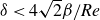 $\delta \lt 4\sqrt 2\beta / \textit{Re}$
and any
$\delta \lt 4\sqrt 2\beta / \textit{Re}$
and any $1 \leq a \lt 2\delta (1-1/\varLambda )/ \textit{Wi}$
the estimate
$1 \leq a \lt 2\delta (1-1/\varLambda )/ \textit{Wi}$
the estimate
 \begin{align} \varLambda \frac {\mathrm{d} V}{\mathrm{d} t} \leq -c_1 \left (\left \lVert \boldsymbol{\nabla }\boldsymbol{v} \right \rVert ^2 + \left \lVert \unicode{x1D659} \right \rVert ^2_{\unicode{x1D659}}\right ) + c_2 \end{align}
holds for some positive constants $c_1, c_2$
(i.e.
$c_1, c_2$
(i.e. $\delta$
and
$\delta$
and $a$
are chosen so as not to quite absorb all the dissipative terms). It then follows from (4.3) that
$a$
are chosen so as not to quite absorb all the dissipative terms). It then follows from (4.3) that
 \begin{align} \frac {\mathrm{d} V}{\mathrm{d} t} \leq -c V + \gamma \end{align}
for some $c,\gamma \gt 0$
along trajectories of the system, and we can conclude from Grönwall’s lemma that
$c,\gamma \gt 0$
along trajectories of the system, and we can conclude from Grönwall’s lemma that $V$
is bounded along trajectories. Since (4.28) holds, condition (ii) of Lemma1 holds with
$V$
is bounded along trajectories. Since (4.28) holds, condition (ii) of Lemma1 holds with
 \begin{align} \kappa = \frac {\varLambda \beta }{4\delta Re} + (2- \sqrt 2) \frac {\varLambda (1-\beta )}{\textit{a {Re Wi}}}, \end{align}
and the final bound is computed by substituting the choices (4.29) into the above equation. This completes the proof of Theorem1.
Appendix D. Proof of Theorem 2
Proof. It is shown in (Binns & Wynn Reference Binns and Wynn2024) that, if
 \begin{align} \alpha = \left (1- \textit{Wi}\right ) \left (1 - \frac {Wi}{\sqrt {1+ \textit{Wi}^2}}\right ) ,\end{align}
then $ \unicode{x1D644} + \alpha \unicode{x1D659} \succeq \unicode{x1D644}-\alpha \unicode{x1D658}_{\textit{steady}} \succ 0$
.
$ \unicode{x1D644} + \alpha \unicode{x1D659} \succeq \unicode{x1D644}-\alpha \unicode{x1D658}_{\textit{steady}} \succ 0$
.
If $ \unicode{x1D658}$
is bounded along trajectories of the system, we have that
$ \unicode{x1D658}$
is bounded along trajectories of the system, we have that
 \begin{align} \overline {\frac {\mathrm{d} }{\mathrm{d} t} \int _\varOmega \log \det \unicode{x1D658} \;\mathrm{d} V} = \frac {1}{ \textit{Wi}} \overline {\int _\varOmega \mathrm{tr}\left ( \unicode{x1D658}^{-1} - \unicode{x1D644}\right ) \;\mathrm{d} V} = 0. \end{align}
This motivates studying the quantity
 \begin{align} \tilde {\mathcal{E}} = \frac {\beta }{ Re} \left \lVert \boldsymbol{\nabla }\boldsymbol{u} \right \rVert ^2 + \frac {1-\beta }{{2 \textit{Re Wi}}^2} \int _\varOmega \mathrm{tr}( \unicode{x1D658} - \unicode{x1D644}\kern1.5pt) \;\mathrm{d} V \end{align}
since its time average is equal to the time-averaged dissipation rate of the overall system $\overline {\mathcal{E}}$
. We now use the fact that
$\overline {\mathcal{E}}$
. We now use the fact that $\|\boldsymbol{\nabla }\boldsymbol{u}\|^2 = \|\boldsymbol{\nabla }\boldsymbol{v}\|^2 + \|\boldsymbol{\nabla }\boldsymbol{b}\|^2$
(since
$\|\boldsymbol{\nabla }\boldsymbol{u}\|^2 = \|\boldsymbol{\nabla }\boldsymbol{v}\|^2 + \|\boldsymbol{\nabla }\boldsymbol{b}\|^2$
(since $\boldsymbol{b}=\boldsymbol{b}_{\textit{steady}}$
) to decompose
$\boldsymbol{b}=\boldsymbol{b}_{\textit{steady}}$
) to decompose $\tilde {\mathcal{E}}$
as
$\tilde {\mathcal{E}}$
as
 \begin{align} \tilde {\mathcal{E}}& = \frac {\beta }{ Re} \left \lVert \boldsymbol{\nabla }\boldsymbol{b} \right \rVert ^2 + \frac {1-\beta }{{2 \textit{Re Wi}}^2} \int _\varOmega \mathrm{tr}( \unicode{x1D658}_b - \unicode{x1D644}\kern1.5pt) \;\mathrm{d} V + \underbrace {\frac {\beta }{ Re} \left \lVert \boldsymbol{\nabla }\boldsymbol{v} \right \rVert ^2_2 + \frac {1-\beta }{{2 \textit{Re Wi}}^2} \int _\varOmega \mathrm{tr}( \unicode{x1D659}\kern1.5pt) \;\mathrm{d} V}_{\mathcal{E}_{2}} \nonumber\\ & = \frac {1}{ Re} + \mathcal{E}_2. \end{align}
We now aim to control $\mathcal{E}_2$
using an appropriately chosen auxiliary functional
$\mathcal{E}_2$
using an appropriately chosen auxiliary functional $V$
whose derivative is given by (4.11). It was shown in (Binns & Wynn Reference Binns and Wynn2024) that within the region
$V$
whose derivative is given by (4.11). It was shown in (Binns & Wynn Reference Binns and Wynn2024) that within the region
 \begin{align} \frac {\mathrm{tr}( \unicode{x1D644} - \alpha \unicode{x1D658}_b)}{\alpha \textit{Wi}} \left (\frac {1-\beta }{1- \textit{Wi}} \right ) \textit{Wi} + \frac { Re}{ Re_E} \lt \beta , \end{align}
if $V$
is defined with
$V$
is defined with $\boldsymbol{b} = \boldsymbol{b}_{\textit{steady}}$
and
$\boldsymbol{b} = \boldsymbol{b}_{\textit{steady}}$
and $ \unicode{x1D658}_b= \unicode{x1D658}_{\textit{steady}}$
given by (4.7), then
$ \unicode{x1D658}_b= \unicode{x1D658}_{\textit{steady}}$
given by (4.7), then
 \begin{align} \frac {\mathrm{d} V}{\mathrm{d} t} \leq -\varepsilon _1 \left \lVert \alpha \unicode{x1D659} \right \rVert ^2_{\alpha \unicode{x1D659}} - \varepsilon _2 \left \lVert \boldsymbol{\nabla }\boldsymbol{v} \right \rVert ^2_2, \end{align}
for some constants $\varepsilon _1,\varepsilon _2\gt 0$
which depend on the system parameters. This also shows that
$\varepsilon _1,\varepsilon _2\gt 0$
which depend on the system parameters. This also shows that $ \unicode{x1D659}$
and
$ \unicode{x1D659}$
and $ \unicode{x1D658}$
are bounded along trajectories of the system, whenever (D5) holds. Using (D6) gives
$ \unicode{x1D658}$
are bounded along trajectories of the system, whenever (D5) holds. Using (D6) gives
 \begin{align} \mathcal{E}_2 + \varLambda \frac {\mathrm{d} V}{\mathrm{d} t} \leq \left ( \frac {\beta }{ Re} - \varLambda \epsilon _2 \right ) \left \lVert \boldsymbol{\nabla }\boldsymbol{v} \right \rVert ^2_2+ \frac {1-\beta }{2\alpha \textit{Re Wi}^2} \int _\varOmega \mathrm{tr}(\alpha \unicode{x1D659}\kern1.5pt) \;\mathrm{d} V - \varLambda \varepsilon _1 \left \lVert \alpha \unicode{x1D659} \right \rVert ^2_{\alpha \unicode{x1D659}} ,\end{align}
where we are free to pick the constant $\varLambda$
. Writing
$\varLambda$
. Writing $\gamma = 2\alpha \textit{Re Wi}^2 \varLambda \epsilon _1 / (1-\beta )$
and using the identity
$\gamma = 2\alpha \textit{Re Wi}^2 \varLambda \epsilon _1 / (1-\beta )$
and using the identity $\| \unicode{x1D63C}-\unicode{x1D644} \kern0.5pt \|_{ \unicode{x1D63C}-\unicode{x1D644}}^2 = \int_\Omega \mathrm{tr}{\left ( \unicode{x1D63C} + \unicode{x1D63C}^{-1}-2 \unicode{x1D644}\kern1.5pt \right )}\,{\mathrm{d} V}$
, we have
$\| \unicode{x1D63C}-\unicode{x1D644} \kern0.5pt \|_{ \unicode{x1D63C}-\unicode{x1D644}}^2 = \int_\Omega \mathrm{tr}{\left ( \unicode{x1D63C} + \unicode{x1D63C}^{-1}-2 \unicode{x1D644}\kern1.5pt \right )}\,{\mathrm{d} V}$
, we have
 \begin{align} \mathcal{E}_2 + \varLambda \frac {\mathrm{d} V}{\mathrm{d} t} &\leq \left ( \frac {\beta }{ Re} - \varLambda \epsilon _2 \right ) \left \lVert \boldsymbol{\nabla }\boldsymbol{v} \right \rVert ^2_2 \end{align}
 \begin{align} &\quad +\frac {1-\beta }{2\alpha \textit{Re Wi}^2} \int _\varOmega \mathrm{tr}( \unicode{x1D644}+\alpha \unicode{x1D659}\kern1.5pt) - \mathrm{tr}{ \unicode{x1D644}} \; - \gamma \mathrm{tr} \left [ {( \unicode{x1D644}+\alpha \unicode{x1D659}\kern1.5pt)^{-1} + ( \unicode{x1D644}+\alpha \unicode{x1D659}\kern1.5pt) - 2 \unicode{x1D644}} \right ] \mathrm{d} V \end{align}
 \begin{align} & = \left ( \frac {\beta }{ Re} - \varLambda \epsilon _2 \right ) \left \lVert \boldsymbol{\nabla }\boldsymbol{v} \right \rVert ^2_2 +\frac {1-\beta }{2\alpha \textit{Re Wi}^2} \sum _{i\,=\,1}^3 \int _\varOmega f_\gamma (\lambda _i) \mathrm{d} V \end{align}
where $\lambda _i\gt 0$
are the (necessarily positive) eigenvalues of
$\lambda _i\gt 0$
are the (necessarily positive) eigenvalues of $ \unicode{x1D644}+\alpha \unicode{x1D659}$
and
$ \unicode{x1D644}+\alpha \unicode{x1D659}$
and $f_\gamma$
is the function
$f_\gamma$
is the function
 \begin{align} f_\gamma (x) = x -1 - \gamma (x + x^{-1}-2), \qquad x\gt 0. \end{align}
If $\gamma \gt 1$
, elementary calculus implies that
$\gamma \gt 1$
, elementary calculus implies that $f_\gamma$
has a maximum at
$f_\gamma$
has a maximum at $x = \sqrt {\gamma /(\gamma -1)}$
with maximum value
$x = \sqrt {\gamma /(\gamma -1)}$
with maximum value
 \begin{align} \max _{x\,\gt\, 0} f_\gamma (x) = 2\gamma -1 - 2\sqrt {\gamma (\gamma -1)} = \frac {1}{2\gamma -1 + 2\sqrt {\gamma (\gamma -1)}} \leq \frac {1}{\gamma }. \end{align}
Using this inequality in (D10) gives
 \begin{align} \mathcal{E}_2 + \varLambda \frac {\mathrm{d} V}{\mathrm{d} t}& \leq \left ( \frac {\beta }{ Re} - \varLambda \epsilon _2 \right ) \left \lVert \boldsymbol{\nabla }\boldsymbol{v} \right \rVert ^2_2 +\frac {3(1-\beta )}{2\alpha \textit{Re Wi}^2 \gamma } \nonumber\\ &=\left ( \frac {\beta }{ Re} - \varLambda \epsilon _2 \right ) \left \lVert \boldsymbol{\nabla }\boldsymbol{v} \right \rVert ^2_2 + \frac {3}{\varLambda \epsilon _1} \left (\frac {(1-\beta )}{2\alpha \textit{Re Wi}^2 }\right )^2. \end{align}
Consequently, if $\varLambda$
is sufficiently large then there is a constant
$\varLambda$
is sufficiently large then there is a constant $c\gt 0$
, independent of
$c\gt 0$
, independent of $\varLambda$
for which
$\varLambda$
for which
 \begin{align} \mathcal{E}_2 + \varLambda \frac {\mathrm{d} V}{\mathrm{d} t} \leq \frac {c}{\varLambda }. \end{align}
Substituting this expression into (D4) gives
 \begin{align} \tilde {\mathcal{E}} + \varLambda \frac {\mathrm{d} V}{\mathrm{d} t} \leq \frac {1}{ Re} + \frac {c}{\varLambda }. \end{align}
Taking the time average of this expression, and using the fact $\overline {\mathcal{E}} = \overline {\tilde {\mathcal{E}}}$
, gives the required bound.
$\overline {\mathcal{E}} = \overline {\tilde {\mathcal{E}}}$
, gives the required bound.
Appendix E. Proof of (5.4)
Proof.
We first write $ \unicode{x1D658}$
in terms of its principal leading submatrix
$ \unicode{x1D658}$
in terms of its principal leading submatrix $ \unicode{x1D658}_{2\times 2}$
 \begin{align} \unicode{x1D658} = \begin{bmatrix} \unicode{x1D658}_{2\times 2} & \unicode{x1D662}\\ \unicode{x1D662}^\top &c_{zz} \end{bmatrix}, \qquad \unicode{x1D662} = \begin{bmatrix} c_{xz}\\ c_{yz} \end{bmatrix}, \qquad \unicode{x1D658}_{2\times 2} = \begin{bmatrix} c_{xx} & c_{xy}\\ c_{xy} & 1 \end{bmatrix}. \end{align}
With no-penetration and no-slip boundary conditions in the $\boldsymbol{e}_y$
direction, we consider the streamwise shear component
$\boldsymbol{e}_y$
direction, we consider the streamwise shear component
 \begin{align} S = \left . \frac {\partial u_x}{\partial y} \right |_{{wall}} \end{align}
and the governing equations for the components of $ \unicode{x1D658}_{2\times 2}$
at the walls
$ \unicode{x1D658}_{2\times 2}$
at the walls
 \begin{align} \frac {\partial c_{xx}}{\partial t} = 2S \,c_{xy} + \frac {1-c_{xx}}{ \textit{Wi}}, \qquad \frac {\partial c_{xy}}{\partial t} = S\, c_{yy} - \frac {c_{xy}}{ \textit{Wi}}, \qquad \frac {\partial c_{yy}}{\partial t} = \frac {1-c_{yy}}{ \textit{Wi}}. \end{align}
Hence,
 \begin{align} c_{yy} (t) = 1 + \left (c_{yy}(0) -1 \right )e^{-t/ \textit{Wi}} \to 1, \qquad \text{as} \; t \rightarrow \infty . \end{align}
We now assume $c_{yy} = 1$
initially, so that it remains so for all subsequent times. We now analyse the behaviour of the leading principal submatrix at the walls and define itsdeterminant as
$c_{yy} = 1$
initially, so that it remains so for all subsequent times. We now analyse the behaviour of the leading principal submatrix at the walls and define itsdeterminant as
 \begin{align} \varDelta = c_{xx} - c_{xy}^2. \end{align}
The time derivative of the determinant is given by
 \begin{align} \dot {\varDelta } = \frac {\partial c_{xx}}{\partial t} - 2c_{xy} \frac {\partial c_{xy}}{\partial t} = -\frac {c_{xx}-1}{ \textit{Wi}} + \frac {2c_{xy}^2}{ \textit{Wi}} = \frac {1}{ \textit{Wi}} \left (1 + c_{xy}^2 - \varDelta \right ), \end{align}
which gives the equality
 \begin{align} c_{xy}^2 = (\varDelta -1 ) + \textit{Wi}\, \dot {\varDelta }. \end{align}
By utilising the above equalities we obtain
 \begin{align} \begin{split} \left .\mathrm{tr}\left ( \unicode{x1D658}_{2\times 2} + \unicode{x1D658}_{2\times 2}^{-1} - 2 \unicode{x1D644}_{2\times 2}\right )\right |_{{wall}} &= c_{xx} -3 + \frac {1 + c_{xx}}{\varDelta }\\ &= \left (\varDelta + c_{xy}^2 -3 \right ) + \frac {1+\varDelta + c_{xy}^2}{\varDelta }\\ &= \left (\varDelta + \frac {1}{\varDelta } -2\right ) + c_{xy}^2 \left (1+ \frac {1}{\varDelta } \right )\\ &= \left (\varDelta + \frac {1}{\varDelta } -2\right ) + \left [(\varDelta -1) + \textit{Wi}\,\dot {\varDelta } \right ] \left (1 + \frac {1}{\varDelta } \right )\\ &= 2(\varDelta - 1) + \textit{Wi}\left (\dot {\varDelta } + \frac {\dot {\varDelta }}{\varDelta }\right ). \end{split} \end{align}
By noticing that
 \begin{align} \dot {\varDelta } + \frac {\dot {\varDelta }}{\varDelta } = \frac {\mathrm{d} }{\mathrm{d} t} \left (\varDelta + \log \varDelta \right ) \end{align}
and utilising the property of infinite-time averages
 \begin{align} \overline {\left .\mathrm{tr}\left ( \unicode{x1D658}_{2\times 2} + \unicode{x1D658}_{2\times 2}^{-1} - 2 \unicode{x1D644}_{2\times 2}\right )\right |_{{wall}}} = 2\left (\overline {\varDelta }-1\right ) + \textit{Wi} \overline {\frac {\mathrm{d} }{\mathrm{d} t} \left (\varDelta + \log \varDelta \right )} = 2\left (\overline {\varDelta }-1\right ). \end{align}
Similarly, we find
 \begin{align} \overline {c_{xy}^2} = \overline {\varDelta } -1 + \textit{Wi}\overline {\dot {\varDelta }} = \overline {\varDelta } -1, \end{align}
which leads to
 \begin{align} 2\overline {c_{xy}^2} = \overline {\left .\mathrm{tr}\left ( \unicode{x1D658}_{2\times 2} + \unicode{x1D658}_{2\times 2}^{-1} - 2 \unicode{x1D644}_{2\times 2}\right )\right |_{{wall}}}. \end{align}
The final step then involves proving
 \begin{align} \overline {\left .\mathrm{tr}\left ( \unicode{x1D658}_{2\times 2} + \unicode{x1D658}_{2\times 2}^{-1} - 2 \unicode{x1D644}_{2\times 2}\right )\right |_{{wall}}} \leq \overline {\left .\mathrm{tr}\left ( \unicode{x1D658} + \unicode{x1D658}^{-1} - 2 \unicode{x1D644}\right )\right |_{{wall}}}. \end{align}
We consider the decomposition
 \begin{align} \mathrm{tr}\left ( \unicode{x1D658} + \unicode{x1D658}^{-1} - 2 \unicode{x1D644}\right ) = \mathrm{tr}\left ( \unicode{x1D658}_{2\times 2} + \left ( \unicode{x1D658}^{-1}\right )_{2\times 2} - 2 \unicode{x1D644}_{2\times 2}\right ) +\left [c_{zz} + \left ( \unicode{x1D658}^{-1}\right )_{zz} -2\right ]. \end{align}
For a positive-definite matrix $ \unicode{x1D658}$
, the properties of Schur complements (Horn & Johnson Reference Horn and Johnson2013, Theorem 7.7.15) imply that
$ \unicode{x1D658}$
, the properties of Schur complements (Horn & Johnson Reference Horn and Johnson2013, Theorem 7.7.15) imply that
 \begin{align} \left ( \unicode{x1D658} ^{-1}\right )_{2\times 2} \succeq \unicode{x1D658}_{2\times 2}^{-1} ,\end{align}
and thus
 \begin{align} \mathrm{tr}\left [\left ( \unicode{x1D658} ^{-1}\right )_{2\times 2} \right ] \geq \mathrm{tr}\left ( \unicode{x1D658}_{2\times 2}^{-1} \right ). \end{align}
Similarly we find
 \begin{align} \left ( \unicode{x1D658}^{-1} \right )_{zz} \geq \frac {1}{c_{zz}}. \end{align}
Hence, from the above estimates and (E14) we have
 \begin{align} \mathrm{tr}\left ( \unicode{x1D658} + \unicode{x1D658}^{-1} - 2 \unicode{x1D644}\right )& \geq \mathrm{tr}\left ( \unicode{x1D658}_{2\times 2} + \unicode{x1D658}^{-1}_{2\times 2} - 2 \unicode{x1D644}_{2\times 2}\right ) + \left (c_{zz} + \frac {1}{c_{zz}} -2 \right )\\ \nonumber &\geq \mathrm{tr}\left ( \unicode{x1D658}_{2\times 2} + \unicode{x1D658}^{-1}_{2\times 2} - 2 \unicode{x1D644}_{2\times 2}\right ). \end{align}
Combining the above inequality with (E12) gives
 \begin{align} 2\overline {c_{xy}^2} \leq \overline {\left .\mathrm{tr}\left ( \unicode{x1D658} + \unicode{x1D658}^{-1} - 2 \unicode{x1D644}\right )\right |_{\textit{wall}}} ,\end{align}
as desired.
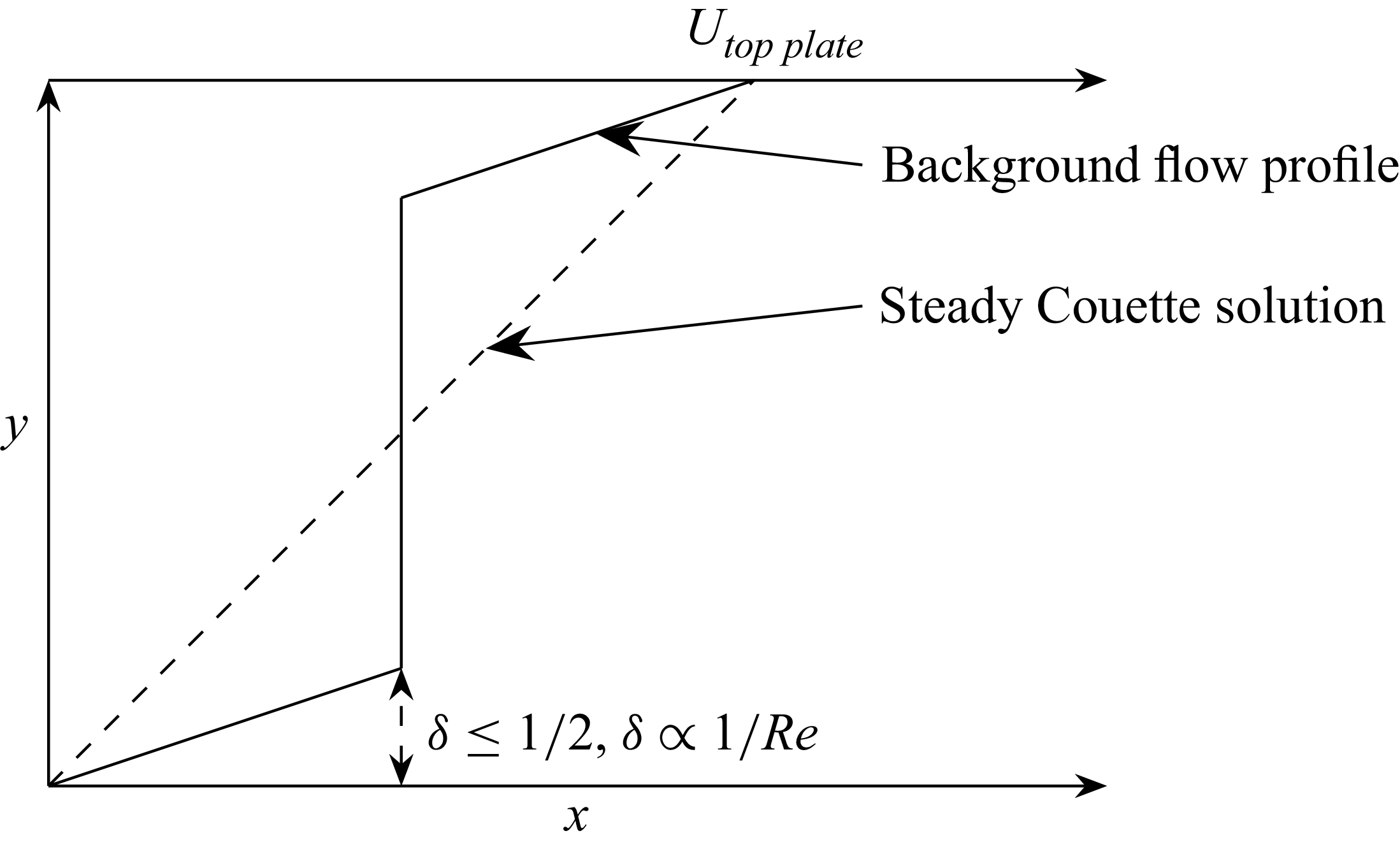
 δ
δ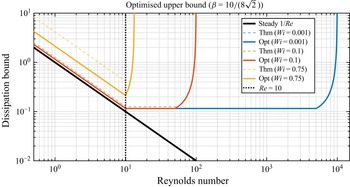
 Re
Re E¯
E¯ β=10/(82)
 1/Re
1/Re Re=82β=10
 Open access

