


1. Introduction
Interfaces between regions distinguished by contrasting levels of turbulence, buoyancy or potential vorticity have both a kinematic and dynamical influence of the flow (da Silva et al. Reference da Silva, Hunt, Eames and Westerweel2014). For example, the continuously deforming interface at the edge of a turbulent jet leads to entrainment and dilution within the jet flow, and acts as a kinematic barrier to transport. The sharp interfaces associated with vortex sheets shed from bluff bodies, or that evolve into trailing vortices from lifting surfaces, play a crucial dynamical role in the force experienced by rigid bodies. There have been significant advances in identifying salient features of these interfaces, especially for turbulent–non-turbulent interfaces, where the interfacial processes are expressed in conditionally averaged flow properties (Westerweel et al. Reference Westerweel, Fukushima, Pedersen and Hunt2009; van Reeuwijk & Holzner Reference van Reeuwijk and Holzner2014). Attention has now shifted towards interfaces between turbulent regions (typically referred to as turbulent–turbulent interfaces or TTIs – see Kohan & Gaskin Reference Kohan and Gaskin2024), a nascent area where there remain significant conceptual gaps in how the turbulence on both sides adjusts in time (Kankanwadi & Buxton Reference Kankanwadi and Buxton2022). The present paper provides insight into the adjustment across an interface between a coherent structure and an external turbulent field (see figure 1(a) and Khojasteh et al. Reference Khojasteh, van Dalen, Been, Westerweel and van de Water2025), in an effort to understand how the permanent local and non-local adjustments occur, following up a former investigation on the interactions between a spherical vortex and ambient turbulent (Eames & Flór Reference Eames and Flór2024).
In a quiescent flow, a compact three-dimensional vortex generates a weak downstream vortical wake flow due to the loss of vorticity by (turbulent) diffusion (Maxworthy Reference Maxworthy1974, Reference Maxworthy1977). The flow around the front and sides of the vortex is irrotational, with the near field flow being dipolar as a consequence of kinematic blocking, and the far field being monopolar as a consequence of the reduction of the vortex impulse. The external turbulence plays an important dynamical role on the vortex by enhancing the loss of impulse causing the vortex to slow down (Eames & Flór Reference Eames and Flór2024). The influence of external turbulence on the vortex is illustrated in figure 1(a), which shows a time sequence of a vortex moving through a turbulent flow where the fluid within the vortex contains a fluorescent dye and is illuminated with a laser-light sheet. The image shows the loss of material at the vortex rear, and this loss leads to a reduction of the vortex impulse and ultimately its arrest. Part of the challenge in understanding the effect of turbulence on the interface between the coherent structure (within the vortex) and the external flow is how the external turbulence is modified.
(a) Photograph showing a vortex that has moved into a turbulent flow. A schematic of the distortion of an external turbulent eddy is shown for times $t_1$
,
$t_1$
, $t_2$
and
$t_2$
and $t_3$
(where
$t_3$
(where $t_3\gt t_2\gt t_1$
). The experimental set-up is described by Eames & Flór (Reference Eames and Flór2024). (b) A regime diagram, expressed in terms of turbulent intensity
$t_3\gt t_2\gt t_1$
). The experimental set-up is described by Eames & Flór (Reference Eames and Flór2024). (b) A regime diagram, expressed in terms of turbulent intensity $I_t=u_0/U_0$
and integral scale
$I_t=u_0/U_0$
and integral scale ${\mathcal L}=L/R_0$
, is shown with the experimental data points of Arnold, Klettner & Eames (Reference Arnold, Klettner and Eames2013) (squares) and Eames & Flór (Reference Eames and Flór2024) (crosses and triangles represent numerical simulations and experimental results, respectively). The current numerical simulations are represented by circles. Here,
${\mathcal L}=L/R_0$
, is shown with the experimental data points of Arnold, Klettner & Eames (Reference Arnold, Klettner and Eames2013) (squares) and Eames & Flór (Reference Eames and Flór2024) (crosses and triangles represent numerical simulations and experimental results, respectively). The current numerical simulations are represented by circles. Here, $\varLambda = {\mathcal L}/I_t$
is the ratio of the eddy turnover time to the advective time scale past the vortex, and
$\varLambda = {\mathcal L}/I_t$
is the ratio of the eddy turnover time to the advective time scale past the vortex, and $\alpha = 2\,Re_t/Re_0$
is the ratio of the Reynolds number of the vortex to the turbulence, expressed by
$\alpha = 2\,Re_t/Re_0$
is the ratio of the Reynolds number of the vortex to the turbulence, expressed by $\alpha ={\mathcal L} I_t$
. The shaded region indicates the parameter space where rapid distortion theory (RDT) is approximately valid.
$\alpha ={\mathcal L} I_t$
. The shaded region indicates the parameter space where rapid distortion theory (RDT) is approximately valid.

Rigid boundaries profoundly alter turbulence through kinematic blocking and the imposition of the no-slip condition. These effects suppress velocity fluctuations normal to the wall while enhancing fluctuations parallel to the surface. The initial near-wall adjustment was modelled by Hunt & Graham (Reference Hunt and Graham1978), accounting for viscous effects and the no-slip constraint. When turbulence encounters a rigid surface – either from an incident stream interacting with a bluff body or under a straining flow – it is distorted by the mean flow. The nature of the distortion depends on the relative scales of the turbulent structures and the straining region (Hunt Reference Hunt1973). Vorticity components perpendicular to the mean flow are preferentially stretched, a mechanism explored through a rapid distortion analysis.
The response of turbulence to a uniform flow past a rigid body was examined in classical analyses by Hunt (Reference Hunt1973), Hunt & Graham (Reference Hunt and Graham1978) and others, and later extended by Durbin (Reference Durbin1981) to axisymmetric flows. These studies primarily focused on the upstream adjustment region, where the mean flow tends towards irrotational behaviour. In contrast, turbulence modification by vortical structures has been investigated through studies of columnar vortices – motivated by atmospheric persistence phenomena (e.g. aircraft wake vortices) and the destabilising effects of stretched vortices wrapping around a vortex core (Myiazaki & Hunt Reference Myiazaki and Hunt2000). The adjustment of turbulence by a spherical vortex is quite different from a line vortex, because fluid elements are not continously stretched and the flow perturbation is localised.
The aim of this paper is to examine how a spherical vortex modifies ambient turbulence, extending earlier work that focused on how turbulence influences vortex propagation. To understand this reciprocal interaction, it is necessary to characterise how the external vorticity field is altered by both distortion and displacement – fundamental processes in all turbulent interface dynamics. The paper is structured as follows: the mathematical model is described in § 2 Two modelling approaches are applied, the first based on an inviscid analysis approach and the second based on a viscous model, are described in § 3. One way to represent the external turbulence is through the superposition of random Fourier modes. The fundamental interaction with a single Fourier mode is assessed in § 4 and extended to multiple modes in § 5. The permanent change of the turbulent field is assessed, with the distinction made between the local and non-local response. Finally, the findings are put in a broader context in § 6, highlighting implications for turbulent interface dynamics more generally.
2. Mathematical model
2.1. Key dimensionless groups
To begin analysing the key mechanisms governing the interaction, it is helpful to identify the relevant dimensionless groups. The theoretical configuration considered is that of a spherical vortex moving through homogeneous turbulence. The principal dimensional parameters are the initial vortex velocity $ U_0$
, the vortex radius
$ U_0$
, the vortex radius $ R_0$
, and the turbulence characteristics: the integral length scale
$ R_0$
, and the turbulence characteristics: the integral length scale $ L$
and the root mean square velocity
$ L$
and the root mean square velocity $ u_0$
. Two characteristic Reynolds numbers are defined: one for the vortex,
$ u_0$
. Two characteristic Reynolds numbers are defined: one for the vortex, $ Re_0 = 2U_0R_0/\nu$
, and one for the ambient turbulence,
$ Re_0 = 2U_0R_0/\nu$
, and one for the ambient turbulence, $ Re_t = u_0L/\nu$
, where
$ Re_t = u_0L/\nu$
, where $\nu$
is the kinematic viscosity of the fluid. The Reynolds number associated with the ambient turbulence can be recast as
$\nu$
is the kinematic viscosity of the fluid. The Reynolds number associated with the ambient turbulence can be recast as $Re_t = ({1/2}) \varLambda I_t\, Re_0$
. The primary dimensionless parameters controlling the interaction are the ratio of turbulence to vortex length scales,
$Re_t = ({1/2}) \varLambda I_t\, Re_0$
. The primary dimensionless parameters controlling the interaction are the ratio of turbulence to vortex length scales, $ \mathcal{L} = L/R_0$
, and the turbulent intensity
$ \mathcal{L} = L/R_0$
, and the turbulent intensity $ I_t = u_0/U_0$
. Figure 1(b) presents a regime diagram incorporating water channel experiments from Arnold (Reference Arnold1976, Reference Arnold2016) and the experimental and numerical turbulence study Eames & Flór (Reference Eames and Flór2024). The latter investigated flows with higher turbulent intensities sufficient to arrest the vortex motion, thereby motivating their exploration of regimes with larger values of
$ I_t = u_0/U_0$
. Figure 1(b) presents a regime diagram incorporating water channel experiments from Arnold (Reference Arnold1976, Reference Arnold2016) and the experimental and numerical turbulence study Eames & Flór (Reference Eames and Flór2024). The latter investigated flows with higher turbulent intensities sufficient to arrest the vortex motion, thereby motivating their exploration of regimes with larger values of $ I_t$
compared to those of Arnold (Reference Arnold2016). The ratio of the turbulent eddy turnover time to the vortex advection time scale is defined as
$ I_t$
compared to those of Arnold (Reference Arnold2016). The ratio of the turbulent eddy turnover time to the vortex advection time scale is defined as $\varLambda = (L/u_{0}) / (R_0/U_0)$
. When
$\varLambda = (L/u_{0}) / (R_0/U_0)$
. When $ \varLambda \gg 1$
and
$ \varLambda \gg 1$
and $ I_t \lt 0.05$
, the external turbulence is rapidly distorted by the flow induced by the vortex, establishing a regime where rapid distortion theory is likely to be applicable.
$ I_t \lt 0.05$
, the external turbulence is rapidly distorted by the flow induced by the vortex, establishing a regime where rapid distortion theory is likely to be applicable.
2.2. Problem definition
The turbulence–vortex model of Eames & Flór (Reference Eames and Flór2024) is briefly described. A Hill’s spherical vortex (Hill Reference Hill1894) moves into a region of homogeneous turbulence that starts a distance $X_c$
from the vortex origin. The incompressible flow
$X_c$
from the vortex origin. The incompressible flow $\boldsymbol{u}$
evolves according to the differential form of the conservation of momentum and mass (with pressure
$\boldsymbol{u}$
evolves according to the differential form of the conservation of momentum and mass (with pressure $p$
and fluid density
$p$
and fluid density $\rho _f$
), described by
$\rho _f$
), described by
 \begin{equation} { {\partial } \boldsymbol{u} \over {\partial } t} + \boldsymbol{u} \boldsymbol{\cdot }\boldsymbol{\nabla } \boldsymbol{u} = - {1\over \rho _f} \boldsymbol{\nabla } p + \nu\, {\nabla }^2 \boldsymbol{u}, \quad \boldsymbol{\nabla } \boldsymbol{\cdot }\boldsymbol{u} =0.\end{equation}
The initial flow $\boldsymbol{u}(\boldsymbol{x},0)=\boldsymbol{u}_v+\boldsymbol{u}_t$
is a superposition of the flow due to a spherical vortex (
$\boldsymbol{u}(\boldsymbol{x},0)=\boldsymbol{u}_v+\boldsymbol{u}_t$
is a superposition of the flow due to a spherical vortex ( $\boldsymbol{u}_v$
) and homogeneous turbulent field (
$\boldsymbol{u}_v$
) and homogeneous turbulent field ( $\boldsymbol{u}_t$
) in a region starting in front of the vortex. The vortex flow
$\boldsymbol{u}_t$
) in a region starting in front of the vortex. The vortex flow $\boldsymbol{u}_v=(u_r,u_\theta )$
is set to be a Hill’s spherical vortex (Hill Reference Hill1894); the flow outside the vortex corresponds to the irrotational flow past a sphere that corresponds to a dipole in an unbounded flow. The initial homogeneous turbulent flow is created from a sum of random Fourier modes (see Kraichnan Reference Kraichnan1959; Fung et al. Reference Fung, Hunt, Malik and Perkins1992), i.e.
$\boldsymbol{u}_v=(u_r,u_\theta )$
is set to be a Hill’s spherical vortex (Hill Reference Hill1894); the flow outside the vortex corresponds to the irrotational flow past a sphere that corresponds to a dipole in an unbounded flow. The initial homogeneous turbulent flow is created from a sum of random Fourier modes (see Kraichnan Reference Kraichnan1959; Fung et al. Reference Fung, Hunt, Malik and Perkins1992), i.e.
 \begin{equation} \boldsymbol{u}_t(\boldsymbol{x}) = \sum _{n=1}^{N_m} \boldsymbol{a}_n \times \hat {\boldsymbol{k}}_n \cos (\boldsymbol{k}_n \boldsymbol{\cdot }\boldsymbol{x} + \psi _n)\,H(x-X_c), \end{equation}
so that the flow is incompressible, where $\psi _n$
is a random phase, and
$\psi _n$
is a random phase, and $\boldsymbol{k}_n$
is a wavenumber of magnitude
$\boldsymbol{k}_n$
is a wavenumber of magnitude $k_n$
with a random direction. Here,
$k_n$
with a random direction. Here, $\boldsymbol{a}_n$
is chosen so that the velocity field has the statistical properties of a prescribed von Kármán energy spectrum
$\boldsymbol{a}_n$
is chosen so that the velocity field has the statistical properties of a prescribed von Kármán energy spectrum $E(k)/u_r^2=f(kL/2\pi )$
(see Cambon, Coleman & Mansour Reference Cambon, Coleman and Mansour1993), where
$E(k)/u_r^2=f(kL/2\pi )$
(see Cambon, Coleman & Mansour Reference Cambon, Coleman and Mansour1993), where $u_r$
is chosen to ensure that the root mean square speed is
$u_r$
is chosen to ensure that the root mean square speed is $u_0$
, and
$u_0$
, and $k$
is the wavenumber (Fung et al. Reference Fung, Hunt, Malik and Perkins1992). The Heaviside step function
$k$
is the wavenumber (Fung et al. Reference Fung, Hunt, Malik and Perkins1992). The Heaviside step function $H$
is set to have value 1 for
$H$
is set to have value 1 for $x\gt X_c$
, and
$x\gt X_c$
, and $0$
for
$0$
for $x\lt X_c$
, ensuring that the vortex is initialised in a quiescent region. The vorticity field associated with (2.2) is
$x\lt X_c$
, ensuring that the vortex is initialised in a quiescent region. The vorticity field associated with (2.2) is $ {\boldsymbol{\omega}}_t(\boldsymbol{x}) = \boldsymbol{\nabla } \times \boldsymbol{u}_t$
, where
$ {\boldsymbol{\omega}}_t(\boldsymbol{x}) = \boldsymbol{\nabla } \times \boldsymbol{u}_t$
, where
 \begin{equation} {\boldsymbol{\omega}}_t(\boldsymbol{x}) = \sum _{n=1}^{N_m}(- \boldsymbol{a}_n k_n + (\boldsymbol{a}_n \boldsymbol{\cdot }\boldsymbol{k}_n) \hat {\boldsymbol{k}}_n ) \sin (\boldsymbol{k}_n \boldsymbol{\cdot }\boldsymbol{x} + \psi _n)\,H(x-X_c), \end{equation}
ensuring that $\boldsymbol{\nabla } \boldsymbol{\cdot }{\boldsymbol{\omega}}_t =0.$
This corrects the typographical error in (3.8) of Eames & Flór (Reference Eames and Flór2024). The artefact of the step change in the velocity field, leading to a vortex sheet at
$\boldsymbol{\nabla } \boldsymbol{\cdot }{\boldsymbol{\omega}}_t =0.$
This corrects the typographical error in (3.8) of Eames & Flór (Reference Eames and Flór2024). The artefact of the step change in the velocity field, leading to a vortex sheet at $x=X_c$
, is not included in (2.3).
$x=X_c$
, is not included in (2.3).
The modification of the external flow is evaluated by comparing the velocity field $\boldsymbol{u}$
, which includes both the vortex and turbulence, with the reference field
$\boldsymbol{u}$
, which includes both the vortex and turbulence, with the reference field $\boldsymbol{u}_{T}$
obtained by initialising the simulation with turbulence alone. The difference between these two fields,
$\boldsymbol{u}_{T}$
obtained by initialising the simulation with turbulence alone. The difference between these two fields,
 \begin{equation} \Delta \boldsymbol{u}=\boldsymbol{u}-\boldsymbol{u}_{T}, \end{equation}
quantifies the influence of the vortex on the surrounding turbulence. The vorticity associated with flow perturbation is $\Delta \boldsymbol{\omega } = \boldsymbol{\nabla } \times \Delta \boldsymbol{u}$
. The external turbulence is affected by the manner in which the flow is strained and displaced. Fluid particles were tagged in the flow, and their position
$\Delta \boldsymbol{\omega } = \boldsymbol{\nabla } \times \Delta \boldsymbol{u}$
. The external turbulence is affected by the manner in which the flow is strained and displaced. Fluid particles were tagged in the flow, and their position $\boldsymbol{X}_p$
was followed by integrating
$\boldsymbol{X}_p$
was followed by integrating
 \begin{equation} {\textrm {d} \boldsymbol{X}_p \over \textrm {d} t }= \boldsymbol{u}(\boldsymbol{X}_p,t) \end{equation}
in time.
(a) The distortion and displacement of slender cylindrical vortex tubes ( $\omega _s$
,
$\omega _s$
, $\omega _n$
,
$\omega _n$
, $\omega _\phi$
) by the irrotational flow past a sphere are shown in red, blue and black, respectively, and lie parallel to, perpendicular to and ’around’ the propagation direction. (b) Comparison between the distortion of a grid of fluid particles by a propagating vortex (
$\omega _\phi$
) by the irrotational flow past a sphere are shown in red, blue and black, respectively, and lie parallel to, perpendicular to and ’around’ the propagation direction. (b) Comparison between the distortion of a grid of fluid particles by a propagating vortex ( $I_t=0$
) and by the potential flow around a growing sphere. The green particles are associated with the displacement caused by a freely moving vortex, while the red particles are associated with the potential flow around a sphere that is moving according to (5.1) and whose radius grows linearly with time (see 5.3).
$I_t=0$
) and by the potential flow around a growing sphere. The green particles are associated with the displacement caused by a freely moving vortex, while the red particles are associated with the potential flow around a sphere that is moving according to (5.1) and whose radius grows linearly with time (see 5.3).

2.3. Numerical simulations
Equations (2.1a,b ) were solved using OpenFOAMv2112 (www.openfoam.com), which is a general computational framework for solving multiphysics problems using a finite-volume method. The flow perturbations (2.4) were evaluated in time by evolving two simulations within the same solver. The simulations were performed using Lagrangian fluid particle tracking, where the particles were seeded randomly both inside the vortex and placed in a structured grid in front of the vortex.
For the vortex–turbulence interaction, the domain size was $ 30R_0 \times W \times W$
, where the domain width is
$ 30R_0 \times W \times W$
, where the domain width is $W=8R_0$
. The cross-sectional area of the channel is
$W=8R_0$
. The cross-sectional area of the channel is $A_{xs} = W^2$
. The vortex is initialised at distance
$A_{xs} = W^2$
. The vortex is initialised at distance $3R_0$
from the inlet plane, with
$3R_0$
from the inlet plane, with $X_c/R_0 = 2$
. The mesh consists of a uniform block with cell numbers
$X_c/R_0 = 2$
. The mesh consists of a uniform block with cell numbers $1000 \times 260 \times 260$
and total cell count 67.6 million. Slip boundary conditions were applied to the walls of the domain, and the simulations ran to time
$1000 \times 260 \times 260$
and total cell count 67.6 million. Slip boundary conditions were applied to the walls of the domain, and the simulations ran to time $\tilde {t}\ (= U_0t/R_0)=50$
.
$\tilde {t}\ (= U_0t/R_0)=50$
.
3. Rapid distortion of external turbulence
Figure 2(b) shows the distortion of a grid of fluid particles (presented in green) by the movement of a freely moving vortex in a quiescent region, and is compared with the distortion of a grid of fluid particles (presented in red) by the flow past a growing Hill’s spherical vortex, with the external flow corresponding to the irrotational flow past a sphere. The displacement of the fluid particles outside the vortex is quite similar in both cases, but there are noticeable differences. Fluid particles are clearly drawn into the rear of the vortex, where they are rapidly circulated; fluid particles close to the centreline are laterally displaced, which is indicative of the loss of impulse.
The movement of a strong vortex into weak turbulence ( $I_t\ll 1$
) leads to the distortion and displacement of the external turbulent field. Broadly speaking, provided that the flow remains inertially dominated and the external vorticity is weak, the external flow around the vortex rapidly distorts the vorticity field
$I_t\ll 1$
) leads to the distortion and displacement of the external turbulent field. Broadly speaking, provided that the flow remains inertially dominated and the external vorticity is weak, the external flow around the vortex rapidly distorts the vorticity field ${\boldsymbol{\omega}}_t$
. The rapid distortion model (Hunt Reference Hunt1973; Durbin Reference Durbin1981; Hunt & Carruthers Reference Hunt and Carruthers1990) is introduced along with a discussion of its range of applicability. In the far field, the distortion of the turbulence is weak, and the adjustment comes purely from the displacement field, or reflux.
${\boldsymbol{\omega}}_t$
. The rapid distortion model (Hunt Reference Hunt1973; Durbin Reference Durbin1981; Hunt & Carruthers Reference Hunt and Carruthers1990) is introduced along with a discussion of its range of applicability. In the far field, the distortion of the turbulence is weak, and the adjustment comes purely from the displacement field, or reflux.
3.1. Asymptotic limit $I_t\rightarrow 0$

Upstream of the vortex, the vorticity of the external turbulent field is initially ${\boldsymbol{\omega}}_d(\boldsymbol{x}, 0) = {\boldsymbol{\omega}}_t(\boldsymbol{x})$
. The distortion and displacement of external vorticity
${\boldsymbol{\omega}}_d(\boldsymbol{x}, 0) = {\boldsymbol{\omega}}_t(\boldsymbol{x})$
. The distortion and displacement of external vorticity ${\boldsymbol{\omega}}_d$
by the passage of the vortex (
${\boldsymbol{\omega}}_d$
by the passage of the vortex ( $\boldsymbol{U}= \boldsymbol{u}_v - \boldsymbol{U}_v$
) can be understood using a model that accounts for advection and stretching caused by the flow outside the vortex and diffusion, and is described by
$\boldsymbol{U}= \boldsymbol{u}_v - \boldsymbol{U}_v$
) can be understood using a model that accounts for advection and stretching caused by the flow outside the vortex and diffusion, and is described by
 \begin{eqnarray} \frac {\partial \boldsymbol{ \omega }_d}{\partial t} + \boldsymbol{\nabla } \boldsymbol{\cdot }( \boldsymbol{U} {\boldsymbol{\omega}}_{d}) &=& ({\boldsymbol{\omega}}_d \boldsymbol{\cdot }\boldsymbol{\nabla }) \boldsymbol{U} + \nu\, {\nabla } ^2 {\boldsymbol{\omega}}_d. \end{eqnarray}
The model is based on the eddy turnover time of the external flow ( $L/u_0$
) being longer than the advective time scale (
$L/u_0$
) being longer than the advective time scale ( $R_0/U_0$
) of the vortex, which can be recast as
$R_0/U_0$
) of the vortex, which can be recast as $I_t \ll {\mathcal L}$
or
$I_t \ll {\mathcal L}$
or $\varLambda \gg 1$
. Diffusion causes the vorticity magnitude to decrease; for the change in the vortical field as it passes the spherical vortex to be negligible, the advective time scale
$\varLambda \gg 1$
. Diffusion causes the vorticity magnitude to decrease; for the change in the vortical field as it passes the spherical vortex to be negligible, the advective time scale $R_0/U_0$
must be shorter than the diffusive time scales
$R_0/U_0$
must be shorter than the diffusive time scales $L^2/\nu$
and
$L^2/\nu$
and $R_0^2/\nu$
. Since
$R_0^2/\nu$
. Since ${\mathcal L} \gg 1$
, this constraint reduces to
${\mathcal L} \gg 1$
, this constraint reduces to $Re_0 \gg 1$
. A final constraint is that the vortex must be much stronger than the flow induced by the turbulence, which requires
$Re_0 \gg 1$
. A final constraint is that the vortex must be much stronger than the flow induced by the turbulence, which requires $I_t \ll 1$
, so that we may expect the vortex to move along a straight line. These constraints (
$I_t \ll 1$
, so that we may expect the vortex to move along a straight line. These constraints ( $I_t \ll 1$
,
$I_t \ll 1$
, $Re_0\gg 1$
,
$Re_0\gg 1$
, ${\mathcal L}\gg 1$
) provide an indication of the applicability of the rapid distortion analysis, as shown in figure 1(b). The inviscid limit occurs when
${\mathcal L}\gg 1$
) provide an indication of the applicability of the rapid distortion analysis, as shown in figure 1(b). The inviscid limit occurs when $Re_0\rightarrow \infty$
, where the distorted vorticity satisfies
$Re_0\rightarrow \infty$
, where the distorted vorticity satisfies
 \begin{equation} { \textrm {D} {\boldsymbol{\omega}}_d \over \textrm {D} t} = ({\boldsymbol{\omega}}_d\boldsymbol{\cdot }\boldsymbol{\nabla }) \boldsymbol{U}. \end{equation}
Equation (3.2) can be solved by noting that the vector spanning two fluid particles, $\mathrm{d}\boldsymbol{l}$
, is stretched in the same manner as a vortex line. The vorticity of a fluid element
$\mathrm{d}\boldsymbol{l}$
, is stretched in the same manner as a vortex line. The vorticity of a fluid element ${\boldsymbol{\omega}}_t$
and its initial length
${\boldsymbol{\omega}}_t$
and its initial length $\textrm {d}l_0$
are related to the extension and rotation of an infinitesimal fluid element (Batchelor & Proudman Reference Batchelor and Proudman1954; Hunt Reference Hunt1973) through
$\textrm {d}l_0$
are related to the extension and rotation of an infinitesimal fluid element (Batchelor & Proudman Reference Batchelor and Proudman1954; Hunt Reference Hunt1973) through
 \begin{equation} {\boldsymbol{\omega}}_d = | {\boldsymbol{\omega}}_t| {\textrm {d} \boldsymbol{l}\over \textrm {d}l_0}. \end{equation}
The (initial external) flow past the Hill’s spherical vortex ( $\boldsymbol{U}$
) corresponds to the irrotational flow past a sphere. The maximum azimuthal vorticity lies on the outer edge of the vortex. Cross-stream diffusion, coupled with the significant strain at the rear stagnation point, leads to vorticity being swept downstream and spreading laterally. The primary effect of the wake vorticity is to cause the vortex to slow down due to the loss of impulse (Maxworthy Reference Maxworthy1974). To explore the influence of the vortex on the external turbulence,
$\boldsymbol{U}$
) corresponds to the irrotational flow past a sphere. The maximum azimuthal vorticity lies on the outer edge of the vortex. Cross-stream diffusion, coupled with the significant strain at the rear stagnation point, leads to vorticity being swept downstream and spreading laterally. The primary effect of the wake vorticity is to cause the vortex to slow down due to the loss of impulse (Maxworthy Reference Maxworthy1974). To explore the influence of the vortex on the external turbulence, $\boldsymbol{U}$
is set to be the irrotational flow past a fixed sphere.
$\boldsymbol{U}$
is set to be the irrotational flow past a fixed sphere.
The irrotational flow past a vortex is characterised by two stagnation points and a circumferential region where the flow speed is faster than the vortex speed due to blocking. There is significant strain at the front (and rear) of the spherical vortex leading to differential advection and tilting of fluid elements. The fluid elements initially parallel to the streamlines are compressed as they pass close to the stagnation point, and are stretched where the flow is faster than the ambient (see figure 2(a) with $\omega _s$
). The blocking leads to circular hoop stretching (see figure 2(a) with
$\omega _s$
). The blocking leads to circular hoop stretching (see figure 2(a) with $\omega _\phi$
) as it passes over the sphere. The displacement and distortion of fluid particles by an irrotational flow depend only on the distance moved by the body (vortex), so the inviscid rapid distortion applies to unsteady vortex motion when the results are expressed in terms of the relative movement of the vortex.
$\omega _\phi$
) as it passes over the sphere. The displacement and distortion of fluid particles by an irrotational flow depend only on the distance moved by the body (vortex), so the inviscid rapid distortion applies to unsteady vortex motion when the results are expressed in terms of the relative movement of the vortex.
3.2. Unbounded potential flow around a rigid sphere
Durbin (Reference Durbin1981) analysed the distortion of turbulence around the front of a rigid sphere. We derive the Durbin (Reference Durbin1981) result using the more intuitive method of Hunt (Reference Hunt1973) based on (3.3). The following discussion concerns the axisymmetric potential flow past a sphere (of fixed radius $R_0$
) in an unbounded flow, which needs to be later reconciled with the fact that the flow is bounded. The Stokes stream function
$R_0$
) in an unbounded flow, which needs to be later reconciled with the fact that the flow is bounded. The Stokes stream function $\varPsi = - U_0 r^2 \sin ^2 \theta\, (1-(R_0/r)^3)$
, describing the irrotational flow past a sphere, is constant on a streamline (where
$\varPsi = - U_0 r^2 \sin ^2 \theta\, (1-(R_0/r)^3)$
, describing the irrotational flow past a sphere, is constant on a streamline (where $u_r = -(1/r^2 \sin \theta )\, \partial \varPsi / \partial \theta$
,
$u_r = -(1/r^2 \sin \theta )\, \partial \varPsi / \partial \theta$
, $u_\theta = (1/r\sin \theta )\, \partial \varPsi / \partial r$
) and is related to the ultimate distance of a fluid particle from the centreline,
$u_\theta = (1/r\sin \theta )\, \partial \varPsi / \partial r$
) and is related to the ultimate distance of a fluid particle from the centreline, $\rho _0$
(using the notation of Lighthill Reference Lighthill1956), where
$\rho _0$
(using the notation of Lighthill Reference Lighthill1956), where
 \begin{equation} \rho _0 =(-2\varPsi /U_0)^{1/2}= r \sin \theta \left ( 1-\left ({ R_0\over r}\right )^3\right )^{1/2}. \end{equation}
The point $\boldsymbol{x}=(x,y,z)$
in the vicinity of the vortex is related to the position of a fluid particle
$\boldsymbol{x}=(x,y,z)$
in the vicinity of the vortex is related to the position of a fluid particle $\boldsymbol{X=}(X,Y,Z)$
through
$\boldsymbol{X=}(X,Y,Z)$
through
 \begin{equation} X = x + U_0 t - X_d (x,\rho _0), \quad Y = {y \rho _0 \over (y^2 +z^2)^{1/2}}, \quad Z = {z \rho _0 \over (y^2 +z^2)^{1/2}}. \end{equation}
The streamwise drift of the fluid particle is
 \begin{equation} X_d(x,\rho _0) = \int _\infty ^x \left ( 1+{U_0\over U_x}\right ) \textrm {d} x \end{equation}
(see Darwin Reference Darwin1953; Lighthill Reference Lighthill1956; Eames, Belcher & Hunt Reference Eames, Belcher and Hunt1994). Although the displacement field is cast in terms of time (in (3.5)), it depends exclusively on the relative movement of the fluid particle with respect to the sphere through $X_v=\int _0^t U_v\, \textrm {d}t$
, and applies to unsteady rectilinear motion. The drift volume associated with the vortex is
$X_v=\int _0^t U_v\, \textrm {d}t$
, and applies to unsteady rectilinear motion. The drift volume associated with the vortex is $C_mV_0$
, where the added-mass coefficient is
$C_mV_0$
, where the added-mass coefficient is $C_m=1/2$
, and
$C_m=1/2$
, and $V_0=4\pi R_0^3/3$
is the volume of the spherical vortex. The change of the external vorticity can be related to how fluid line elements (that span two fluid particles) are distorted or deflected (through (3.2)). A fluid line element
$V_0=4\pi R_0^3/3$
is the volume of the spherical vortex. The change of the external vorticity can be related to how fluid line elements (that span two fluid particles) are distorted or deflected (through (3.2)). A fluid line element $\textrm {d}\boldsymbol{l} = \hat {\boldsymbol{x}}$
(e.g. the red tube in figure 2
a) remains parallel to the streamlines, but the length of the fluid line element depends on the local speed:
$\textrm {d}\boldsymbol{l} = \hat {\boldsymbol{x}}$
(e.g. the red tube in figure 2
a) remains parallel to the streamlines, but the length of the fluid line element depends on the local speed:
 \begin{equation} \textrm {d}\boldsymbol{l}_{s} = {q\over U_{vo}} \hat {\boldsymbol{s}}\, \textrm {d}l_0. \end{equation}
A fluid element that is initially in the azimuthal direction ( $\textrm {d}\boldsymbol{l}_\varphi = \textrm {d}l_0\, \hat {\boldsymbol{\varphi }}$
) is stretched as it is pushed away from the centreline so that
$\textrm {d}\boldsymbol{l}_\varphi = \textrm {d}l_0\, \hat {\boldsymbol{\varphi }}$
) is stretched as it is pushed away from the centreline so that
 \begin{equation} \textrm {d}\boldsymbol{l}_\varphi = {\rho \over \rho _0} \hat {\boldsymbol{\varphi }}\,\textrm {d}l_0, \end{equation}
and this is shown as the black hoop in figure 2(a). When a fluid line element is initially perpendicular to the streamline and in the radial direction, corresponding to the blue tube in figure 2(a), i.e. $\textrm {d} \boldsymbol{l} = \hat {\boldsymbol{n}} \textrm { d}l_0$
, it is deformed as
$\textrm {d} \boldsymbol{l} = \hat {\boldsymbol{n}} \textrm { d}l_0$
, it is deformed as
 \begin{equation} \textrm {d}\boldsymbol{l}_n = \left (-{q\over U_0}{\partial X_d\over \partial \rho _0} \hat {\boldsymbol{s}} + {\rho _0 U_{vo}\over q \rho } \hat {\boldsymbol{\rho }}\right ) \textrm {d} l_0, \end{equation}
where $q = |\boldsymbol{u}|$
. With (3.2), the local vorticity field
$q = |\boldsymbol{u}|$
. With (3.2), the local vorticity field ${\boldsymbol{\omega}}_d(\boldsymbol{x},t) = (\omega _{ds}, \omega _{dn}, \omega _{d\varphi })$
can be related to the upstream vorticity field
${\boldsymbol{\omega}}_d(\boldsymbol{x},t) = (\omega _{ds}, \omega _{dn}, \omega _{d\varphi })$
can be related to the upstream vorticity field ${\boldsymbol{\omega}}_t(\boldsymbol{X})$
through
${\boldsymbol{\omega}}_t(\boldsymbol{X})$
through
 \begin{equation} {\boldsymbol{\omega}}_d (\boldsymbol{x},t) = {\omega }_{ts} (\boldsymbol{X})\, { \textrm {d} \boldsymbol{l} _s \over \textrm {d} l_0} +{\omega }_{tn}(\boldsymbol{X})\, { \textrm {d} \boldsymbol{l} _n \over \textrm {d} l_0} +{\omega }_{t\varphi }(\boldsymbol{X})\, { \textrm {d} \boldsymbol{l}_{\varphi } \over \textrm {d} l_0}, \end{equation}
and using (3.7), (3.8) and (3.9), it can be expressed in matrix notation as
 \begin{equation} {\boldsymbol{\omega}}_d= \boldsymbol{\mathrm{A}} \left [ \begin{array}{c} \omega _{tx} \\ \omega _{t\rho } \\ \omega _{t \varphi } \end{array} \right ] , \quad \boldsymbol{\mathrm{A}} = \left [ \begin{array}{ccc} {\dfrac{q}{U_0}} & -{\dfrac{q}{U_0}} {\dfrac{\partial X_d}{\partial \rho _0}} & 0 \\[8pt] 0 & {\dfrac{\rho _0 U_{vo}}{q \rho }} & 0 \\[5pt] 0 & 0 & {\dfrac{\rho}{\rho _0}}\\ \end{array} \right ] . \end{equation}
The correctness of the approach is confirmed by comparisons with Lighthill (Reference Lighthill1956) and equation (11) from Durbin (Reference Durbin1981) (where $\boldsymbol{\mathrm{A}}=\boldsymbol{{\varGamma }}^{-1}$
), notwithstanding the change of notation and flow direction. Finally, the vorticity field at
$\boldsymbol{\mathrm{A}}=\boldsymbol{{\varGamma }}^{-1}$
), notwithstanding the change of notation and flow direction. Finally, the vorticity field at $\boldsymbol{x}$
needs to be transformed from streamline coordinates to Cartesian coordinates using a series of rotation matrices. Thus given a vorticity distribution
$\boldsymbol{x}$
needs to be transformed from streamline coordinates to Cartesian coordinates using a series of rotation matrices. Thus given a vorticity distribution ${\boldsymbol{\omega}}_t$
in (2.3) upstream of the vortex, the vorticity field
${\boldsymbol{\omega}}_t$
in (2.3) upstream of the vortex, the vorticity field ${\boldsymbol{\omega}}_d$
can be calculated from the expression for displacement (through (3.6)) and distortion (through (3.11)).
${\boldsymbol{\omega}}_d$
can be calculated from the expression for displacement (through (3.6)) and distortion (through (3.11)).
Downstream of the vortex, the apparent change in the vorticity field due to the combination of distortion and displacement is
 \begin{equation} {\boldsymbol{\omega}}_d(\boldsymbol{x})={\boldsymbol{\omega}}_t\bigl(\boldsymbol{x}+(U_0t-X_d)\hat {\boldsymbol{x}}\bigr) -\omega _{t\rho } (\boldsymbol{X})\, \hat {\boldsymbol{\rho }}{\partial X_d\over \partial \rho _0}. \end{equation}
The straining flow past the vortex modifies the radial component of the external vorticity field because it is permanently stretched. The initial radial position of fluid line elements is restored downstream of the vortex ( $\rho /\rho _0\rightarrow 1$
), so there is no permanent change in the azimuthal vorticity. Lighthill (Reference Lighthill1956) examined the change in a uniform upstream vorticity field, aligned perpendicular to the stream, interacting with a sphere. The uniformity of the vorticity field means that it is unaffected by displacement and is changed exclusively by distortion. For
$\rho /\rho _0\rightarrow 1$
), so there is no permanent change in the azimuthal vorticity. Lighthill (Reference Lighthill1956) examined the change in a uniform upstream vorticity field, aligned perpendicular to the stream, interacting with a sphere. The uniformity of the vorticity field means that it is unaffected by displacement and is changed exclusively by distortion. For ${\boldsymbol{\omega}}_t = A \hat {\boldsymbol{z}}$
, the change in the vorticity field (3.12)
${\boldsymbol{\omega}}_t = A \hat {\boldsymbol{z}}$
, the change in the vorticity field (3.12)
 \begin{equation} {\boldsymbol{\omega}}_d -{\boldsymbol{\omega}}_t = - A \cos \theta \lim _{x\rightarrow -\infty } {\partial X_d \over \partial \rho _0}\hat {\boldsymbol{x}} \end{equation}
corresponds to trailing vortices, analogous to those behind a lifting surface and derived by Lighthill (Reference Lighthill1956). In the far field ( $|\rho /R_0|\gg 1$
), the change in the vorticity field comes from the displacement field,
$|\rho /R_0|\gg 1$
), the change in the vorticity field comes from the displacement field,
 \begin{equation} {\boldsymbol{\omega}}_d = {\boldsymbol{\omega}}_t (x+U_0 t-X_d,Y,Z), \end{equation}
where the $U_0t$
term arises from a change between the vortex and laboratory frames of reference.
$U_0t$
term arises from a change between the vortex and laboratory frames of reference.
3.3. Influence of flow boundedness
Vortex stretching due to fluid particle drift occurs primarily along the path of the translating vortex. The effect of the flow being bounded leads to the generation of a return flow. For a vortex moving forwards, the weak return flow leads to finite fluid particle displacement. The influence of the confinement in a rectangular channel (of width $W$
) on the flow is assessed by the method of images to be
$W$
) on the flow is assessed by the method of images to be
 \begin{equation} \boldsymbol{u}_v (x,y,z)= \sum _{j,l=-\infty }^{\infty } \boldsymbol{u}_{v0} ( x,y-jW,z-lW), \end{equation}
where $\boldsymbol{u}_{v0} ( x,y-jH,z-lH)$
is the sum of the flow induced by a dipole of moment
$\boldsymbol{u}_{v0} ( x,y-jH,z-lH)$
is the sum of the flow induced by a dipole of moment
 \begin{equation} \mu = {1\over 2} R^3 U, \end{equation}
through
 \begin{equation} \boldsymbol{u}_{v0} = \mu \left ( \frac {y^2+z^2-2x^2}{r^5} ,- \frac {3 x y}{r^5}, -\frac {3 x z}{r^5} \right ). \end{equation}
The flow inside the vortex is taken to be the Hills’s spherical vortex model. With this model, the kinematic condition on the sphere of radius $R$
is in error by a factor of
$R$
is in error by a factor of $O((R/W)^3)$
. Although the vortex grows with time, it does not behave in the same manner as a growing rigid sphere because a kinematic constraint is not imposed on the surface of the vortex. The displacement along the surface of the channel (at
$O((R/W)^3)$
. Although the vortex grows with time, it does not behave in the same manner as a growing rigid sphere because a kinematic constraint is not imposed on the surface of the vortex. The displacement along the surface of the channel (at $y=W/2$
,
$y=W/2$
, $z=0$
) by the sphere moving from
$z=0$
) by the sphere moving from $x=X_o$
to
$x=X_o$
to $x=-X_o$
is
$x=-X_o$
is
 \begin{equation} X_r \approx \int _{-X_o}^{X_o} {\boldsymbol{u}_{v0} \boldsymbol{\cdot }\hat {\boldsymbol{x}} \over U_0}\, \textrm {d}x. \end{equation}
When $R_0$
is constant, the reflux (3.18) is approximately
$R_0$
is constant, the reflux (3.18) is approximately
 \begin{equation} X_r=-{2\mu \over U_0 } \sum _{j,l=-\infty }^\infty {X_o \over (X_o^2 + (y+jW)^2 + (z+lW)^2 )^{3/2}}, \end{equation}
and scales as
 \begin{equation} X_r = -{\lambda (1+C_m)V \over W^2 }, \end{equation}
in the limit of $\tilde{X}_o=X_o/M\gg 1$
, using the Taylor (Reference Taylor1928) expression of the relationship between dipole moment and body volume (
$\tilde{X}_o=X_o/M\gg 1$
, using the Taylor (Reference Taylor1928) expression of the relationship between dipole moment and body volume ( $\mu = (1+C_m) VU_0/4\pi$
). Numerical evaluation of the expression gives
$\mu = (1+C_m) VU_0/4\pi$
). Numerical evaluation of the expression gives $\lambda =0.9998$
for
$\lambda =0.9998$
for $X_o/W=10$
, close to the theoretical value 1. The volume displaced backwards by reflux,
$X_o/W=10$
, close to the theoretical value 1. The volume displaced backwards by reflux, $X_r$
, balances the volume displaced forwards, which consists of the vortex volume (
$X_r$
, balances the volume displaced forwards, which consists of the vortex volume ( $V$
) and the drift volume (
$V$
) and the drift volume ( $C_mV$
), ensuring, by mass conservation, that
$C_mV$
), ensuring, by mass conservation, that
 \begin{equation} X_r = - {(1+C_m)V_0 \over A_{xs}}, \end{equation}
retrieving (3.20) (where $A_{xs}$
is the cross-sectional area of the channel). The asymptotic limit
$A_{xs}$
is the cross-sectional area of the channel). The asymptotic limit $\lambda \rightarrow 0$
, demonstrated in (3.21), can be recovered by first noting that the summation in (3.19) is
$\lambda \rightarrow 0$
, demonstrated in (3.21), can be recovered by first noting that the summation in (3.19) is $\sim 4\sum _{j=1}^\infty \tilde {X}_o/(\tilde {X}_o^2+j^2)$
(using an approximation for the sum of
$\sim 4\sum _{j=1}^\infty \tilde {X}_o/(\tilde {X}_o^2+j^2)$
(using an approximation for the sum of $1/(a+n^2)^{3/2}$
), and the summation tends to
$1/(a+n^2)^{3/2}$
), and the summation tends to $\sim 2\pi$
. This result closes the discussion by Eames et al. (Reference Eames, Belcher and Hunt1994) of flow boundedness. The general influence of an evolving vortex radius and speed is incorporated in (3.15) and integrated over time.
$\sim 2\pi$
. This result closes the discussion by Eames et al. (Reference Eames, Belcher and Hunt1994) of flow boundedness. The general influence of an evolving vortex radius and speed is incorporated in (3.15) and integrated over time.
3.4. Numerical solution
The rapid distortion models are described by (3.4)–(3.11). The inviscid modes were evaluated in a gridded region ( $|x|\lt 3R_0$
,
$|x|\lt 3R_0$
, $0\lt y \leqslant 3R_0$
,
$0\lt y \leqslant 3R_0$
, $z=0$
) with resolution
$z=0$
) with resolution $300\times 300$
points. The adjustment of (2.3) was evaluated in C++ (programming language) to speed up the computation. The viscous rapid distortion model (3.1) was solved with a bespoke OpenFOAM solver. The vortex-induced flow
$300\times 300$
points. The adjustment of (2.3) was evaluated in C++ (programming language) to speed up the computation. The viscous rapid distortion model (3.1) was solved with a bespoke OpenFOAM solver. The vortex-induced flow $\boldsymbol{U}$
was either specified analytically (for an unbounded flow) or solved using potentialFoam to account for flow boundedness. The vorticity field (3.12) was specified beyond a distance
$\boldsymbol{U}$
was either specified analytically (for an unbounded flow) or solved using potentialFoam to account for flow boundedness. The vorticity field (3.12) was specified beyond a distance $X_c$
from the sphere centre, and the inlet conditions were determined by specifying the sine argument in (2.3) to be
$X_c$
from the sphere centre, and the inlet conditions were determined by specifying the sine argument in (2.3) to be $(\boldsymbol{k}_n\boldsymbol{\cdot }(\boldsymbol{x} + \boldsymbol{U}_v t) +\phi _n)$
so that the vorticity field is swept through the domain. The domain size was reduced to
$(\boldsymbol{k}_n\boldsymbol{\cdot }(\boldsymbol{x} + \boldsymbol{U}_v t) +\phi _n)$
so that the vorticity field is swept through the domain. The domain size was reduced to $6R_0\times 6R_0\times 6R_0$
. To reduce numerical instability,
$6R_0\times 6R_0\times 6R_0$
. To reduce numerical instability, $X_c$
was set to be
$X_c$
was set to be $2R_0$
, to ensure a smooth adjustment in the vorticity field for cases C1, C2 and C3.
$2R_0$
, to ensure a smooth adjustment in the vorticity field for cases C1, C2 and C3.
To eliminate the effect of external vorticity leaking into the vortex, the computational domain was created with the interior of the vortex excluded. This was achieved using a uniform blockmesh and along with snappyHexMesh applied to an stl representation of a sphere, with inflation layers on the spherical boundary. The final mesh contained approximately 4.6 million cells.
4. Vortex moving into a structured vortical flow
The spatial and temporal complexity of a turbulent flow masks the interaction between a propagating vortex and the external turbulence. To unpick this interaction, we first examine how the vortex interacts with a structured flow comprised of a single Fourier mode of (2.2)–(2.3):
 \begin{equation} \boldsymbol{u}_t = \bigl(\boldsymbol{a} \times \hat {\boldsymbol{k}}\bigr) \cos (\boldsymbol{k}\boldsymbol{\cdot }\boldsymbol{x} +\psi ), \quad {\boldsymbol{\omega}}_{t} =\bigl(- \boldsymbol{a} k + (\boldsymbol{a} \boldsymbol{\cdot }\boldsymbol{k}) \hat {\boldsymbol{k}}\bigr) \sin (\boldsymbol{k}\boldsymbol{\cdot }\boldsymbol{x} +\psi ). \end{equation}
The adjustment of the external vortical field depends on whether the vorticity is aligned parallel or perpendicular to the direction of motion of the vortex. Three distinct cases are chosen (cases C1, C2 and C3), as listed in table 1. The wavenumber of the flow is $k=2\pi /L$
; the integral scale takes the values
$k=2\pi /L$
; the integral scale takes the values ${\mathcal L}=1$
, 2 and 4. The phase (
${\mathcal L}=1$
, 2 and 4. The phase ( $\psi$
) is chosen to ensure that
$\psi$
) is chosen to ensure that $\omega _x$
and
$\omega _x$
and $\omega _y$
are not both zero in the
$\omega _y$
are not both zero in the $z=0$
plane. The flow induced by the vortex was chosen to be that associated with an unbounded flow for the theoretical inviscid model and the numerical viscous distortion model. The vorticity is periodically signed, which means that positive and negative vorticity cancel one another through diffusion, leading to the vorticity maximum decreasing as
$z=0$
plane. The flow induced by the vortex was chosen to be that associated with an unbounded flow for the theoretical inviscid model and the numerical viscous distortion model. The vorticity is periodically signed, which means that positive and negative vorticity cancel one another through diffusion, leading to the vorticity maximum decreasing as $\exp ( -t/T)$
, where
$\exp ( -t/T)$
, where $T= 1/(k^2\nu )$
. The effect of strain at the front of the vortex enhances this annihilation process by reducing the local length scale (Hunt & Eames Reference Hunt and Eames2002).
$T= 1/(k^2\nu )$
. The effect of strain at the front of the vortex enhances this annihilation process by reducing the local length scale (Hunt & Eames Reference Hunt and Eames2002).
Characteristics of the structured flows, labelled as C1, C2 and C3, chosen so that $\boldsymbol{a}\boldsymbol{\cdot }\boldsymbol{k}=0$
. The characteristic length scale of the flow is
$\boldsymbol{a}\boldsymbol{\cdot }\boldsymbol{k}=0$
. The characteristic length scale of the flow is $L={2\pi / k}$
, and the values of
$L={2\pi / k}$
, and the values of $L/R_0$
are chosen to be 1, 2 or 4. The characteristic measures are
$L/R_0$
are chosen to be 1, 2 or 4. The characteristic measures are $I_t = |\boldsymbol{a} \times \hat {\boldsymbol{k}}|/\sqrt {2}U_0$
and
$I_t = |\boldsymbol{a} \times \hat {\boldsymbol{k}}|/\sqrt {2}U_0$
and ${\mathcal L}=2\pi /kR_0$
. For the viscous rapid distortion analysis,
${\mathcal L}=2\pi /kR_0$
. For the viscous rapid distortion analysis, $Re_0=2000$
.
$Re_0=2000$
.

4.1. Case C1
Figure 3 shows a comparison between the inviscid (figure 3
a) and viscous (figure 3
b) rapid distortion of a single Fourier mode. The vortex moves perpendicular to $\boldsymbol{k}$
, leading to a displacement and distortion of the iso-contours of
$\boldsymbol{k}$
, leading to a displacement and distortion of the iso-contours of $|{\boldsymbol{\omega}}_t|$
. The distortion leads to a rapid fluctuation of vorticity adjacent to the surface of the sphere, both at the leading stagnation point and along the attached streamline. The production of streamwise vorticity
$|{\boldsymbol{\omega}}_t|$
. The distortion leads to a rapid fluctuation of vorticity adjacent to the surface of the sphere, both at the leading stagnation point and along the attached streamline. The production of streamwise vorticity $\omega _x$
occurs through the tilting of cross-stream vorticity (
$\omega _x$
occurs through the tilting of cross-stream vorticity ( $\omega _y$
), and has the same periodicity downstream of the sphere. Viscous diffusion leads to a reduction in the maximum magnitude of
$\omega _y$
), and has the same periodicity downstream of the sphere. Viscous diffusion leads to a reduction in the maximum magnitude of $\omega _y$
and
$\omega _y$
and $\omega _x$
, particularly where the local wavenumber increases. The effect of increasing the wavelength (
$\omega _x$
, particularly where the local wavenumber increases. The effect of increasing the wavelength ( $L$
) is to reduce the magnitude of the vorticity gradients and lessen diffusive effects for the viscous rapid distortion calculations (contrasting figures 3
a,b).
$L$
) is to reduce the magnitude of the vorticity gradients and lessen diffusive effects for the viscous rapid distortion calculations (contrasting figures 3
a,b).
The vorticity field components $\omega _x/ak$
and
$\omega _x/ak$
and $\omega _y/ak$
, created from the distortion of (4.1) (case C1, see table 1) by the irrotational flow past a sphere, are shown for
$\omega _y/ak$
, created from the distortion of (4.1) (case C1, see table 1) by the irrotational flow past a sphere, are shown for ${\mathcal L}=1, 2, 4$
at
${\mathcal L}=1, 2, 4$
at $\tilde {t}=10$
. The upstream vorticity is parallel to the
$\tilde {t}=10$
. The upstream vorticity is parallel to the $y$
-axis, and the wavenumber is parallel to the
$y$
-axis, and the wavenumber is parallel to the $x$
-axis. The results from the inviscid and viscous rapid distortion analysis are shown in (a) and (b), respectively.
$x$
-axis. The results from the inviscid and viscous rapid distortion analysis are shown in (a) and (b), respectively.

Numerical simulations of a freely moving vortex passing into a structured flow (case C1), characterised by ${\mathcal L}=1$
,
${\mathcal L}=1$
, $Re_0=2000$
and
$Re_0=2000$
and $I_t=0.01$
. The vorticity fields (a)
$I_t=0.01$
. The vorticity fields (a) $\omega _x/ak$
and (b)
$\omega _x/ak$
and (b) $\omega _y/ak$
are shown for
$\omega _y/ak$
are shown for $\tilde {t}=5$
, 10, 20, 30.
$\tilde {t}=5$
, 10, 20, 30.

Figure 4 shows the movement of a vortex into the vorticity field (case C1) with $I_t=0.01$
. The background vorticity field (
$I_t=0.01$
. The background vorticity field ( $\omega _y$
) for
$\omega _y$
) for $k=2\pi /R_0$
decreases over the decay time
$k=2\pi /R_0$
decreases over the decay time $\tilde {T}=Re_0/(2(kR_0)^2)$
, which is approximately 25 and comparable to the run time of the calculations. The displacement of
$\tilde {T}=Re_0/(2(kR_0)^2)$
, which is approximately 25 and comparable to the run time of the calculations. The displacement of $\omega _y$
, outside the vortex, is similar for both the inviscid and viscous calculations. The generation of
$\omega _y$
, outside the vortex, is similar for both the inviscid and viscous calculations. The generation of $\omega _x$
within the vortex (figure 4
a) initially occurs through viscous entrainment, illustrated in figure 2(b), which leads to a relative flow towards the vortex (
$\omega _x$
within the vortex (figure 4
a) initially occurs through viscous entrainment, illustrated in figure 2(b), which leads to a relative flow towards the vortex ( $\tilde {t}=5$
), greatly amplifying
$\tilde {t}=5$
), greatly amplifying $\omega _x$
by stretching the vorticity through the internal strain. The tilting of
$\omega _x$
by stretching the vorticity through the internal strain. The tilting of $\omega _x$
consequently leads to a production of
$\omega _x$
consequently leads to a production of $\omega _y$
within the vortex, which is evident in figure 4 for
$\omega _y$
within the vortex, which is evident in figure 4 for $\tilde {t}=30$
. At a later time, the generation of
$\tilde {t}=30$
. At a later time, the generation of $\omega _x$
within the vortex is a consequence of a re-orientation of
$\omega _x$
within the vortex is a consequence of a re-orientation of $\omega _z$
.
$\omega _z$
.
4.2. Case C2
(a) The vorticity field components $\omega _x/ak$
and
$\omega _x/ak$
and $\omega _y/ak$
calculated from the rapid distortion analysis are shown for case C2 (see table 1) with
$\omega _y/ak$
calculated from the rapid distortion analysis are shown for case C2 (see table 1) with ${\mathcal L} = 2$
at
${\mathcal L} = 2$
at $\tilde {t} = 10$
, for both the inviscid and viscous cases. Here, the external vorticity is parallel to uniform flow with the wavenumber perpendicular to the incident flow. (b) The vorticities in the
$\tilde {t} = 10$
, for both the inviscid and viscous cases. Here, the external vorticity is parallel to uniform flow with the wavenumber perpendicular to the incident flow. (b) The vorticities in the $x$
- and
$x$
- and $y$
-directions are shown at times
$y$
-directions are shown at times $\tilde {t}=5$
, 10, 20 and 30, for
$\tilde {t}=5$
, 10, 20 and 30, for $I_t=0.01$
. The colour scale is shown at the bottom of the figure.
$I_t=0.01$
. The colour scale is shown at the bottom of the figure.

Figure 5(a) shows the rapid adjustment of the vorticity field by the potential flow past a sphere. Since $\omega _t$
is aligned parallel to the incident flow, the vorticity field is simply displaced by the symmetric flow past the sphere, and is affected by the local speed causing the vorticity to be stretched and compressed. Here,
$\omega _t$
is aligned parallel to the incident flow, the vorticity field is simply displaced by the symmetric flow past the sphere, and is affected by the local speed causing the vorticity to be stretched and compressed. Here, $\omega _y$
is reduced in strength at the front and back of the vortex where the local flow is slower, leading to the vorticity being compressed (from (3.7));
$\omega _y$
is reduced in strength at the front and back of the vortex where the local flow is slower, leading to the vorticity being compressed (from (3.7)); $\omega _y$
is created simply by tilting the streamwise vorticity, leading to
$\omega _y$
is created simply by tilting the streamwise vorticity, leading to $\omega _x$
being negative at the front, and positive at the rear, of the vortex. The adjustment in the
$\omega _x$
being negative at the front, and positive at the rear, of the vortex. The adjustment in the $z=0$
plane is weakly dependent on
$z=0$
plane is weakly dependent on $L/R_0$
, justifying the presentation of a single value of
$L/R_0$
, justifying the presentation of a single value of $L/R_0$
. Figure 5(b) shows the adjustment of the vorticity field due to a propagating vortex (
$L/R_0$
. Figure 5(b) shows the adjustment of the vorticity field due to a propagating vortex ( $I_t=0.01$
). The plane
$I_t=0.01$
). The plane $z=0$
corresponds to the maximum value of
$z=0$
corresponds to the maximum value of $\omega _x$
, which decreases in time due to diffusion. As with the inviscid analysis,
$\omega _x$
, which decreases in time due to diffusion. As with the inviscid analysis, $\omega _x$
is proportional to the local speed, so decreases in magnitude at the front of the vortex and increases at its side. Entrainment at the rear of the vortex leads to an enhancement within the vortex. The tilting of
$\omega _x$
is proportional to the local speed, so decreases in magnitude at the front of the vortex and increases at its side. Entrainment at the rear of the vortex leads to an enhancement within the vortex. The tilting of $\omega _x$
leads to production in the
$\omega _x$
leads to production in the $y$
-direction, with this occurring adjacent to the downstream wake.
$y$
-direction, with this occurring adjacent to the downstream wake.
(a) The vorticity field components $\omega _x/ak$
and
$\omega _x/ak$
and $\omega _y/ak$
calculated from the rapid distortion analysis are shown for case C3 (see table 1) with
$\omega _y/ak$
calculated from the rapid distortion analysis are shown for case C3 (see table 1) with ${\mathcal L}=2$
at
${\mathcal L}=2$
at $\tilde {t}=10$
, for both the inviscid and viscous cases. (b) The propagation of a freely moving vortex in the structured flow case C3 is shown at times
$\tilde {t}=10$
, for both the inviscid and viscous cases. (b) The propagation of a freely moving vortex in the structured flow case C3 is shown at times $\tilde {t}=5$
, 10, 20, 30 and 40, with
$\tilde {t}=5$
, 10, 20, 30 and 40, with ${\mathcal L}=1$
.
${\mathcal L}=1$
.

4.3. Case C3
In the plane $z=0$
, the vorticity field
$z=0$
, the vorticity field $\omega _y$
is uniform upstream of the vortex. The production of
$\omega _y$
is uniform upstream of the vortex. The production of $\omega _x$
(see figure 6
a) is through the tilting of
$\omega _x$
(see figure 6
a) is through the tilting of $\omega _y$
caused by the differential advection of fluid particles on adjacent streamlines, which leads to
$\omega _y$
caused by the differential advection of fluid particles on adjacent streamlines, which leads to $\omega _x$
increasing in magnitude. The influence of diffusion tends to smooth out the vorticity at the leading edge of the sphere (see figure 5(a), viscous flow panel).
$\omega _x$
increasing in magnitude. The influence of diffusion tends to smooth out the vorticity at the leading edge of the sphere (see figure 5(a), viscous flow panel).
Figure 6(b) shows the consequence of a freely moving vortex moving through the structured flow. The adjustment of $\omega _x$
for the freely propagating vortex is similar to the rapid distortion analysis around the sides of the vortex and arises from the tilting of the cross-stream vorticity. Vorticity is drawn from the wake into the vortex, where it can be rapidly stretched. At later times, the vortex becomes unstable, and vorticity is shed from the vortex, leading to an observable wake in the rear. The asymmetry across the vortex, for
$\omega _x$
for the freely propagating vortex is similar to the rapid distortion analysis around the sides of the vortex and arises from the tilting of the cross-stream vorticity. Vorticity is drawn from the wake into the vortex, where it can be rapidly stretched. At later times, the vortex becomes unstable, and vorticity is shed from the vortex, leading to an observable wake in the rear. The asymmetry across the vortex, for $\omega _y$
, occurs due to the streamlines not returning to their lateral position as a consequence of the loss of impulse from the vortex.
$\omega _y$
, occurs due to the streamlines not returning to their lateral position as a consequence of the loss of impulse from the vortex.
Comparison between the vortical structures and displacement profiles for cases (a) C1, (b) C2 and (c) C3, for ${\mathcal L}=1$
and
${\mathcal L}=1$
and $I_t=0.01$
. The deformation of the grid of fluid particles (shown in green) is presented alongside the trajectories of the particles that originated within the vortex (shown in red). The vortex is represented as an iso-surface of the second invariant of the velocity gradient tensor
$I_t=0.01$
. The deformation of the grid of fluid particles (shown in green) is presented alongside the trajectories of the particles that originated within the vortex (shown in red). The vortex is represented as an iso-surface of the second invariant of the velocity gradient tensor $II=({1/2}) (\|\boldsymbol{\varOmega } \|^2 - \| \boldsymbol{S} \|^2)$
, where
$II=({1/2}) (\|\boldsymbol{\varOmega } \|^2 - \| \boldsymbol{S} \|^2)$
, where $\boldsymbol{\varOmega }=(\boldsymbol{\nabla }\boldsymbol{u}-(\boldsymbol{\nabla }\boldsymbol{u})^{\rm T})/2$
and
$\boldsymbol{\varOmega }=(\boldsymbol{\nabla }\boldsymbol{u}-(\boldsymbol{\nabla }\boldsymbol{u})^{\rm T})/2$
and $\boldsymbol{S}=(\boldsymbol{\nabla }\boldsymbol{u}+(\boldsymbol{\nabla }\boldsymbol{u})^{\rm T})/2$
(Hunt, Wray & Moin Reference Hunt, Wray and Moin1988); here,
$\boldsymbol{S}=(\boldsymbol{\nabla }\boldsymbol{u}+(\boldsymbol{\nabla }\boldsymbol{u})^{\rm T})/2$
(Hunt, Wray & Moin Reference Hunt, Wray and Moin1988); here, $II=10^{-2}\ \textrm {s}^{-2}$
is used to highlight the propagating vortex. The times are
$II=10^{-2}\ \textrm {s}^{-2}$
is used to highlight the propagating vortex. The times are $\tilde {t} = 5,10,20,30,40$
. The vortex centre and radius are shown in (d) and (e), respectively. The black, red and blue circles correspond to cases C1, C2 and C3, respectively.
$\tilde {t} = 5,10,20,30,40$
. The vortex centre and radius are shown in (d) and (e), respectively. The black, red and blue circles correspond to cases C1, C2 and C3, respectively.

The characteristics of a vortex passing through an unstructured flow are shown, where the model parameters are $N_m=50$
,
$N_m=50$
, ${\mathcal L} = 4$
,
${\mathcal L} = 4$
, $L_{min}/R_0 =0.25 {\mathcal L}$
and
$L_{min}/R_0 =0.25 {\mathcal L}$
and $L_{max}/R_0 = 2 {\mathcal L}$
,
$L_{max}/R_0 = 2 {\mathcal L}$
, $Re_0=2000$
,
$Re_0=2000$
, $I_t=0.01$
,
$I_t=0.01$
, $Re_t=40$
. In (a), the iso-surface
$Re_t=40$
. In (a), the iso-surface $II=10^{-4}\ \textrm {s}^{-2}$
is used to highlight the background turbulence, while the iso-surface
$II=10^{-4}\ \textrm {s}^{-2}$
is used to highlight the background turbulence, while the iso-surface $II=10^{-2}\ \textrm {s}^{-2}$
is used to highlight the propagating vortex. The time instances correspond to
$II=10^{-2}\ \textrm {s}^{-2}$
is used to highlight the propagating vortex. The time instances correspond to $\tilde {t}=5$
, 10, 20, 30 and 40. The distribution of strengths of Fourier modes is shown in (b), with
$\tilde {t}=5$
, 10, 20, 30 and 40. The distribution of strengths of Fourier modes is shown in (b), with $|\boldsymbol{a}_n|/u_0$
plotted as a function of
$|\boldsymbol{a}_n|/u_0$
plotted as a function of $k$
from
$k$
from $2\pi /L_{max}$
to
$2\pi /L_{max}$
to $2\pi /L_{min}$
. In (c,d), the characteristics of the vortex expressed in terms of vortex position and radius are plotted as functions of dimensionless time
$2\pi /L_{min}$
. In (c,d), the characteristics of the vortex expressed in terms of vortex position and radius are plotted as functions of dimensionless time $\tilde {t}$
. The black line corresponds to (5.1); the red dashed line corresponds to a line of best fit.
$\tilde {t}$
. The black line corresponds to (5.1); the red dashed line corresponds to a line of best fit.

Comparison between the vorticity field $\omega _xR_0/U_0I_t$
(in the
$\omega _xR_0/U_0I_t$
(in the $z$
-plane) calculated for (a) a vortex freely moving through an unstructured flow, compared with the rapid distortion analysis based on inviscid and viscous models in (b) and (c), respectively. The unstructured flow is the same in all cases and corresponds to
$z$
-plane) calculated for (a) a vortex freely moving through an unstructured flow, compared with the rapid distortion analysis based on inviscid and viscous models in (b) and (c), respectively. The unstructured flow is the same in all cases and corresponds to $Re_0=2000$
,
$Re_0=2000$
, $N_m = 50$
,
$N_m = 50$
, ${\mathcal L} = 4$
,
${\mathcal L} = 4$
, $L_{min}/R_0 =0.25{\mathcal L}$
and
$L_{min}/R_0 =0.25{\mathcal L}$
and $L_{max}/R_0 = 2 {\mathcal L}$
,
$L_{max}/R_0 = 2 {\mathcal L}$
, $I_t = 0.01$
,
$I_t = 0.01$
, $Re_t=40$
. In (a), the positions of Lagrangian fluid particles, initially located within the vortex, are plotted within a thin slice that includes the
$Re_t=40$
. In (a), the positions of Lagrangian fluid particles, initially located within the vortex, are plotted within a thin slice that includes the $z$
-plane. For (a), the simulation time is indicated, while in (b), the distance moved by the sphere is taken to match the distance moved by the vortex – excursion distance and time are linked through figure 8(c).
$z$
-plane. For (a), the simulation time is indicated, while in (b), the distance moved by the sphere is taken to match the distance moved by the vortex – excursion distance and time are linked through figure 8(c).

Sequence showing the free movement of a vortex into an unstructured flow (shown in figure 8
b) with components (a) $\omega _xR_0/U_0I_t$
and (b)
$\omega _xR_0/U_0I_t$
and (b) $\omega _yR_0/U_0I_t$
in the plane
$\omega _yR_0/U_0I_t$
in the plane $z=0$
, contrasting the cases
$z=0$
, contrasting the cases $I_t=0.05$
(
$I_t=0.05$
( $Re_t=200$
) and
$Re_t=200$
) and $I_t=0.01$
(
$I_t=0.01$
( $Re_t=40$
).
$Re_t=40$
).

Changes to near- and far-field turbulence by the passage of a vortex with $I_t=0.01$
and
$I_t=0.01$
and $Re_0=2000$
. In (a), a series of snapshots of the changes in the vorticity field due to the vortex in the plane
$Re_0=2000$
. In (a), a series of snapshots of the changes in the vorticity field due to the vortex in the plane $z=0$
is shown. The filled contours of
$z=0$
is shown. The filled contours of $\Delta \omega _x/( \boldsymbol{\omega }^2+\delta _\omega ^2)^{1/2}$
are shown. (Here,
$\Delta \omega _x/( \boldsymbol{\omega }^2+\delta _\omega ^2)^{1/2}$
are shown. (Here, $\delta _\omega =10^{-2}$
was chosen to desingularise the normalisation.) In (b,i) and (b,iii), the flow properties along the control surface (at
$\delta _\omega =10^{-2}$
was chosen to desingularise the normalisation.) In (b,i) and (b,iii), the flow properties along the control surface (at $y/R_0=4$
,
$y/R_0=4$
, $z=0$
) are plotted for
$z=0$
) are plotted for $\tilde {t}=30$
, with the streamline vorticity (
$\tilde {t}=30$
, with the streamline vorticity ( $\omega _x$
) and velocity (
$\omega _x$
) and velocity ( $u_x$
) plotted for the case of a vortex freely moving in turbulence (black) and the reference case of turbulence evolving isolation (red). In (b,ii), the velocity difference is compared against the flow induced by a dipole whose moment is constant. In (b,iv),
$u_x$
) plotted for the case of a vortex freely moving in turbulence (black) and the reference case of turbulence evolving isolation (red). In (b,ii), the velocity difference is compared against the flow induced by a dipole whose moment is constant. In (b,iv), $\Delta \omega _x$
is plotted along with
$\Delta \omega _x$
is plotted along with $-X_d(x,t)\,\partial \omega _{xT}/\partial x$
for
$-X_d(x,t)\,\partial \omega _{xT}/\partial x$
for $\tilde {t}=30$
. In (c), the fluid particle displacement is plotted for different times, while in (d), the displacement of the horizontal vorticity field is estimated from the streamwise correlation distance.
$\tilde {t}=30$
. In (c), the fluid particle displacement is plotted for different times, while in (d), the displacement of the horizontal vorticity field is estimated from the streamwise correlation distance.

Figure 7 summarises the different types of interactions with the spherical vortex (with C1, C2 and C3 in respective figures 7
a,b,c), and shows the effect of the interaction on the vortex wake, displacement, size and deformation. The vortex passage is through a grid of Lagrangian particles, whose longitudinal drift and lateral displacement are apparent in figure 7(a–c). All the sequences show a fluid displacement with a characteristic drift profile (similar to figure 2). When the ambient vorticity is aligned parallel to $\boldsymbol{\hat {x}}$
, vortex stretching is largely absent, and the vortex core remains coherent for a longer period. The clear gap in particles behind the vortex gives an indication of the entrainment into the vortex, with this being much larger for C1 and C2, and detrainment of vorticity. The vortices have a strong tendency to decelerate when the vortex appears to become unstable (at
$\boldsymbol{\hat {x}}$
, vortex stretching is largely absent, and the vortex core remains coherent for a longer period. The clear gap in particles behind the vortex gives an indication of the entrainment into the vortex, with this being much larger for C1 and C2, and detrainment of vorticity. The vortices have a strong tendency to decelerate when the vortex appears to become unstable (at $\tilde {t}=20{-}30$
) for cases C1 and C2, as is evident from a change in gradient in figure 7(d). The vortex core radius is plotted as a function of time in figure 7(e).
$\tilde {t}=20{-}30$
) for cases C1 and C2, as is evident from a change in gradient in figure 7(d). The vortex core radius is plotted as a function of time in figure 7(e).
5. Vortex moving into unstructured flow
The analysis is extended to an unstructured flow, comprised of multiple Fourier modes, to understand how the near- and far-field flow is changed by the vortex. This provides an opportunity to unpick the structural changes to the vorticity flow as a consequence of vortex movement. The range of wavenumbers varied from $2\pi /L_{max}$
to
$2\pi /L_{max}$
to $2\pi /L_{min}$
, where
$2\pi /L_{min}$
, where $L_{min}/R_0=0.25 {\mathcal L}$
,
$L_{min}/R_0=0.25 {\mathcal L}$
, $L_{max}/R_0=2{\mathcal L}$
and
$L_{max}/R_0=2{\mathcal L}$
and ${\mathcal L} = 4$
(the same as in Eames & Flór Reference Eames and Flór2024); the upper limit on the wavenumbers was chosen to reduce the effect of diffusion on the smallest scales. The strengths of the Fourier modes in (2.2) are shown in figure 8(b).
${\mathcal L} = 4$
(the same as in Eames & Flór Reference Eames and Flór2024); the upper limit on the wavenumbers was chosen to reduce the effect of diffusion on the smallest scales. The strengths of the Fourier modes in (2.2) are shown in figure 8(b).
5.1. Weak turbulence interaction
Figure 8 shows the movement of a vortex into a turbulent flow for $I_t=0.01$
and
$I_t=0.01$
and $Re_0=2000$
. The position of the vortex and state of the external turbulence are indicated by the second variant, which is the difference between a measure of fluid rotation compared to strain. In the vicinity of the vortex, irrotational strain is increased, leading to noticeable reduction in
$Re_0=2000$
. The position of the vortex and state of the external turbulence are indicated by the second variant, which is the difference between a measure of fluid rotation compared to strain. In the vicinity of the vortex, irrotational strain is increased, leading to noticeable reduction in $II$
(see caption of figure 8) near the vortex, which is evident in figure 8(a). The details of the turbulence are listed in the caption. The position of the vortex as a function of time was determined from the average position of Lagrangian fluid particles, initially released within the vortex,
$II$
(see caption of figure 8) near the vortex, which is evident in figure 8(a). The details of the turbulence are listed in the caption. The position of the vortex as a function of time was determined from the average position of Lagrangian fluid particles, initially released within the vortex, $\langle X_v \rangle$
(figure 8
c), and is compared with Maxworthy’s model with an entrainment coefficient
$\langle X_v \rangle$
(figure 8
c), and is compared with Maxworthy’s model with an entrainment coefficient $\alpha =0.0125$
(see Eames & Flór Reference Eames and Flór2024):
$\alpha =0.0125$
(see Eames & Flór Reference Eames and Flór2024):
 \begin{equation} X_v = {1\over \alpha }\left ( \left ( 1 +6 \alpha U_0t/R_0\right )^{1/6}-1\right ), \quad U_v/U_0 = (R_m/R_0)^{-5}. \end{equation}
The vortex radius $R_m$
is estimated from the maximum excursion of the fluid particles from the centreline, and its variation in time is shown in figure 8(d). A vortex moving through a quiescent flow grows initially at a slower rate until the vortex becomes unstable (beyond
$R_m$
is estimated from the maximum excursion of the fluid particles from the centreline, and its variation in time is shown in figure 8(d). A vortex moving through a quiescent flow grows initially at a slower rate until the vortex becomes unstable (beyond $\tilde {t}\sim 25$
), after which it grows to a size comparable to that shown in the images of figure 8(a).
$\tilde {t}\sim 25$
), after which it grows to a size comparable to that shown in the images of figure 8(a).
To understand the interaction between a freely moving vortex and turbulence, the inviscid and viscous rapid distortion models were applied to the same (synthetic) turbulent flows to determine the adjustment of $\boldsymbol{\omega }$
. The rapid distortion models are based on the sphere or vortex remaining the same size. The time sequence in figure 9(a) shows
$\boldsymbol{\omega }$
. The rapid distortion models are based on the sphere or vortex remaining the same size. The time sequence in figure 9(a) shows $\omega _x$
in the
$\omega _x$
in the $z=0$
plane, with the Lagrangian particles, initially within the vortex, plotted with a thin slice that includes the
$z=0$
plane, with the Lagrangian particles, initially within the vortex, plotted with a thin slice that includes the $z$
-plane. The rapid distortion theory is based on the distance the vortex has penetrated the turbulent field, which is determined by linking the distance the vortex has moved, with time (see figure 8
c). The creation of
$z$
-plane. The rapid distortion theory is based on the distance the vortex has penetrated the turbulent field, which is determined by linking the distance the vortex has moved, with time (see figure 8
c). The creation of $\omega _x$
within the vortex is due to entrainment (evident at
$\omega _x$
within the vortex is due to entrainment (evident at $\tilde {t}=5$
), which is stretched within the vortex and also rearranged through an instability process (figure 7
b). The distortion models in figures 9(b,c) agree with each other, with the noticeable difference explained by the effect of diffusion, which occurs over time
$\tilde {t}=5$
), which is stretched within the vortex and also rearranged through an instability process (figure 7
b). The distortion models in figures 9(b,c) agree with each other, with the noticeable difference explained by the effect of diffusion, which occurs over time $3R_0/U_0$
(the time taken for the fluid to enter the computational domain and reach the vortex position); diffusion operates over a much longer period in figure 9(a), in addition to the turbulent flow evolving in time. The differences evident at
$3R_0/U_0$
(the time taken for the fluid to enter the computational domain and reach the vortex position); diffusion operates over a much longer period in figure 9(a), in addition to the turbulent flow evolving in time. The differences evident at $\tilde {t}=5$
are due to viscous flow calculation running for a finite period of time, and the sphere (vortex) initially starting off surrounded by irrotational fluid before it moves into the turbulent region; the edge between the irrotational and turbulent fluid (due to
$\tilde {t}=5$
are due to viscous flow calculation running for a finite period of time, and the sphere (vortex) initially starting off surrounded by irrotational fluid before it moves into the turbulent region; the edge between the irrotational and turbulent fluid (due to $X_c/R_0=2$
) is denoted as the dashed line. The results for the other vorticity components (
$X_c/R_0=2$
) is denoted as the dashed line. The results for the other vorticity components ( $\omega _y$
and
$\omega _y$
and $\omega _z$
) show similar features. The distortion analysis provides a leading-order description because
$\omega _z$
) show similar features. The distortion analysis provides a leading-order description because $Re_0\gg 1$
, and both
$Re_0\gg 1$
, and both $I_t$
and
$I_t$
and $\mathcal L$
sit within the rapid distortion theory region indicated in the regime diagram of figure 1(b).
$\mathcal L$
sit within the rapid distortion theory region indicated in the regime diagram of figure 1(b).
Figure 10 shows a comparison between a vortex moving into weak and strong turbulence. The initial interactions look quite similar upto $\tilde{t}=10$
. For the strong turbulence the eddy turnover time of the smaller vortices is approximately
$\tilde{t}=10$
. For the strong turbulence the eddy turnover time of the smaller vortices is approximately $L_{min }/u_0 = 2R_0/U_0$
which is comparable to the advective time scale past the vortex. As a result, although the overall turbulent structure is comparable, the finer features in the stronger turbulent flow due to the nonlinear interactions between eddies of different sizes. The rapid distortion interpretation still holds, but it applies primarily to the turbulent field immediately upstream of the vortex.
$L_{min }/u_0 = 2R_0/U_0$
which is comparable to the advective time scale past the vortex. As a result, although the overall turbulent structure is comparable, the finer features in the stronger turbulent flow due to the nonlinear interactions between eddies of different sizes. The rapid distortion interpretation still holds, but it applies primarily to the turbulent field immediately upstream of the vortex.
5.2. Near- and far-field influences
The permanent change to the external turbulent flow, due to the passage of the vortex, is assessed by comparing the evolution of two flows, where the first is initialised with the vortex and turbulence, and the second is initialised with only the turbulence. Figure 11(a) shows a time sequence of the interaction between the vortex and turbulence for $I_t=0.01$
, where the vorticity associated flow perturbation
$I_t=0.01$
, where the vorticity associated flow perturbation $\omega _x$
is normalised by
$\omega _x$
is normalised by $(|\boldsymbol{\omega }|^2+\delta _\omega ^2)^{1/2}$
, where
$(|\boldsymbol{\omega }|^2+\delta _\omega ^2)^{1/2}$
, where $\delta _\omega =10^{-2}$
is used to desingularise the normalisation. This measure highlights the locality of the changes in the vorticity field caused by the vortex. This permanent change is concentrated near the vortex and along the trajectory that it has followed. The vorticity parallel to this trajectory is enhanced downstream due to stretching that tends to align the amplified vorticity with the
$\delta _\omega =10^{-2}$
is used to desingularise the normalisation. This measure highlights the locality of the changes in the vorticity field caused by the vortex. This permanent change is concentrated near the vortex and along the trajectory that it has followed. The vorticity parallel to this trajectory is enhanced downstream due to stretching that tends to align the amplified vorticity with the $x$
-axis. The flow adjustment that occurs ‘far’ from the vortex is explored in figures 11(b,i) and 11(b,iii), which show the variation of
$x$
-axis. The flow adjustment that occurs ‘far’ from the vortex is explored in figures 11(b,i) and 11(b,iii), which show the variation of $u_x$
and
$u_x$
and $\omega _x$
along the line
$\omega _x$
along the line $z=0,\ y=4R_0$
. The red and black lines in figures 11(b,i) and 11(b,iii) differentiate between the vortex being present or absent. The velocity perturbation caused by the vortex is plotted as the black line in figure 11(b,ii). The form of the perturbation indicates that the dipole strength remains unchanged over time; it is compared against the prediction based on the dipole moment (3.16) being constant in time (
$z=0,\ y=4R_0$
. The red and black lines in figures 11(b,i) and 11(b,iii) differentiate between the vortex being present or absent. The velocity perturbation caused by the vortex is plotted as the black line in figure 11(b,ii). The form of the perturbation indicates that the dipole strength remains unchanged over time; it is compared against the prediction based on the dipole moment (3.16) being constant in time ( $\mu =({1/ 2})R_0^3U_0$
). Far from the vortex, the change in the vorticity field (from (3.12)) is
$\mu =({1/ 2})R_0^3U_0$
). Far from the vortex, the change in the vorticity field (from (3.12)) is
 \begin{equation} \Delta \boldsymbol{\omega }={\boldsymbol{\omega}}_d -{\boldsymbol{\omega}}_t\sim {\boldsymbol{\omega}}_t(\boldsymbol{x}-X_d\hat {\boldsymbol{x}})-{\boldsymbol{\omega}}_t(\boldsymbol{x}) \approx -X_d(x,t)\, {\partial {\boldsymbol{\omega}}_t \over \partial x}. \end{equation}
The difference $\Delta \omega _x$
is plotted in figure 11(b,iv) as a black line, and compared with
$\Delta \omega _x$
is plotted in figure 11(b,iv) as a black line, and compared with $-X_d\, {\partial \omega _x/\partial x}$
. The displacement field is evaluated here, assuming that the dipole moment remains unchanged with time but moves according to (5.1). The vortex slows down and grows in size as it moves forward. The fluid displacement along the channel wall is evaluated by including the influence of the vortex growing in size by setting the vortex radius to be
$-X_d\, {\partial \omega _x/\partial x}$
. The displacement field is evaluated here, assuming that the dipole moment remains unchanged with time but moves according to (5.1). The vortex slows down and grows in size as it moves forward. The fluid displacement along the channel wall is evaluated by including the influence of the vortex growing in size by setting the vortex radius to be
 \begin{equation} R_m=R_0(1+\beta \tilde {t}) \end{equation}
(from figure 8(d), with $\beta =0.02$
). The displacement is negative because of the reflux or return flow created by the forward movement of the vortex and the drift volume. The increase in size is taken from the Lagrangian estimates in figure 7(e). Figure 11(c) shows the predicted increase based on the movement of the vortex, which correlates to the simulation times and estimate of
$\beta =0.02$
). The displacement is negative because of the reflux or return flow created by the forward movement of the vortex and the drift volume. The increase in size is taken from the Lagrangian estimates in figure 7(e). Figure 11(c) shows the predicted increase based on the movement of the vortex, which correlates to the simulation times and estimate of $X_d(x)$
shown in figure 11(d). The lateral displacement in the vorticity signature along the channel wall was estimated by calculating the correlation distance between
$X_d(x)$
shown in figure 11(d). The lateral displacement in the vorticity signature along the channel wall was estimated by calculating the correlation distance between $\omega_d$
and
$\omega_d$
and $\omega_t$
, as a function of
$\omega_t$
, as a function of $x/R_0$
. Behind the vortex, the displacement is negative corresponding to reflux; the agreement between the calculations and prediction of lateral displacement is close, as shown by comparing figures 11(c) and 11(d).
$x/R_0$
. Behind the vortex, the displacement is negative corresponding to reflux; the agreement between the calculations and prediction of lateral displacement is close, as shown by comparing figures 11(c) and 11(d).
6. Conclusion
This paper has explored how a spherical vortex modifies turbulence, focusing on the interaction between the vortex-induced flow and the surrounding turbulence. Using a rapid distortion framework, we identified key mechanisms – namely displacement, stretching, and tilting of fluid line elements due to drift gradients – that govern this interaction. Our analysis builds on the foundational work of Hunt and Durbin, while also introducing the previously overlooked role of reflux, a far-field phenomenon that laterally displaces vorticity in a Lagrangian sense. The changes in the turbulent field caused by the vortex have some similarity to the turbulent flow adjacent to the upstream surface of a rigid sphere (see Durbin Reference Durbin1981), but are quite different downstream due to the production of vorticity and shedding caused by the no-slip condition (Bagchi & Balachandar Reference Bagchi and Balachandar2003).
A key outcome of this work is the distinction between local (near-field) and non-local (far-field) effects. In the near field, the vortex distorts turbulence within a region comparable to its own radius, which is analogous to a knife cutting through butter. In the far field, the Eulerian view shows the vortex velocity superimposed on the background flow, whereas the Lagrangian view reveals cumulative displacements due to reflux. Reflux is a manifestation of mass conservation, and this is the non-local response of the vortex on the turbulence, which shows that the far-field effect does not simply diminish to zero.
A TTI is simply a definable interface that lies between two distinct regions with different levels of turbulence, and the edge of a vortex is one such interface. Here we have focused on the permanent change in the external turbulence adjacent to the TTI, and shown how the change in structure can be understood from a Lagrangian perspective that captures the vortex stretching process. Similar processes occur when there is a mean flow relative to a TTI, e.g. at the edge of the entraining turbulent jet. The techniques and ideas developed in this paper may provide a theoretical starting point to explore the production of vorticity in other types of TTI, such as those reported by Kankanwadi & Buxton (Reference Kankanwadi and Buxton2022).
Acknowledgements
The authors acknowledge the Kathleen HPC Facility at University College London for providing computational resources. We thank C. Bordier for facilitating the academic exchange between Université Grenoble Alpes and University College London. We are also grateful to the referees for their constructive comments, which helped to improve the clarity of the manuscript.
Funding
This work was supported by the French National Research Agency (ANR) through the Tec21 project as part of the France 2030 programme (ANR-15-IDEX-0002).
Declaration of interests
The authors report no conflict of interest.
Data availability statement
The data that support the findings of this study are available from the corresponding author I.E. upon reasonable request.


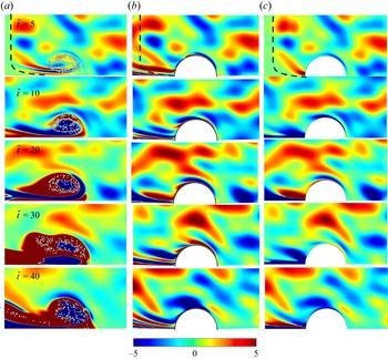


 Open access