


1. Introduction
1.1. Background
The geometrical-optics (GO) approach is widely used for reduced modelling of waves in plasmas and other media (Kravtsov & Orlov Reference Kravtsov and Orlov1990; Tracy et al. Reference Tracy, Brizard, Richardson and Kaufman2014). In this approach, instead of solving the wave equations per se, one converts them into Hamilton’s equations for wave rays and a first-order (in time or the ray path) differential equation for the wave envelope. Then, one calculates the ray trajectories that are relevant to the initial conditions (‘reference rays’) and solves the envelope equations on those trajectories. As an initial-value algorithm, this scheme is computationally inexpensive and has also yielded a number of spinoffs, such as beam tracing (Pereverzev Reference Pereverzev1998; Poli et al. Reference Poli2018; Hall-Chen, Parra & Hillesheim Reference Hall-Chen, Parra and Hillesheim2022) and quasioptics, which can account for both transverse diffraction (Balakin et al. Reference Balakin, Balakina, Permitin and Smirnov2007) and mode conversion (Dodin et al. Reference Dodin, Ruiz, Yanagihara, Zhou and Kubo2019; Yanagihara et al. Reference Yanagihara, Kubo and Dodin2021).Footnote 1
Still, the GO approach is limited in that it assumes that the characteristic scale
 $L$
of the medium is much larger than the local wavelength
$L$
of the medium is much larger than the local wavelength
 $\lambda$
. Even for high-frequency waves, such as those in the electron-cyclotron range, this assumption unavoidably breaks down near cutoffs (reflection points), where
$\lambda$
. Even for high-frequency waves, such as those in the electron-cyclotron range, this assumption unavoidably breaks down near cutoffs (reflection points), where
 $\lambda /L$
is infinite and the conventional GO predicts a spurious singularity of the field amplitude. For example, this is an issue in modelling the O–X mode conversion near the critical plasma density, which is a part of a promising scheme for heating overdense plasmas in fusion reactors (Preinhaelter & Kopecký Reference Preinhaelter and Kopecký1973; Hansen, Lynov & Michelsen Reference Hansen, Lynov and Michelsen1985) and also occurs in the ionosphere (Mjølhus Reference Mjølhus1990; Eliasson & Papadopoulos Reference Eliasson and Papadopoulos2016). Since those waves experience many oscillations during the mode-conversion process, one can expect that some GO-like model should be possible for them, even though the conversion occurs near a cutoff. This motivates a search for alternative formulations of GO that do not rely on the smallness of
$\lambda /L$
is infinite and the conventional GO predicts a spurious singularity of the field amplitude. For example, this is an issue in modelling the O–X mode conversion near the critical plasma density, which is a part of a promising scheme for heating overdense plasmas in fusion reactors (Preinhaelter & Kopecký Reference Preinhaelter and Kopecký1973; Hansen, Lynov & Michelsen Reference Hansen, Lynov and Michelsen1985) and also occurs in the ionosphere (Mjølhus Reference Mjølhus1990; Eliasson & Papadopoulos Reference Eliasson and Papadopoulos2016). Since those waves experience many oscillations during the mode-conversion process, one can expect that some GO-like model should be possible for them, even though the conversion occurs near a cutoff. This motivates a search for alternative formulations of GO that do not rely on the smallness of
 $\lambda /L$
per se.
$\lambda /L$
per se.
One such formulation, which has long been known, is based on Maslov’s approach (Maslov & Fedoriuk Reference Maslov and Fedoriuk1981; Ziolkowski & Deschamps Reference Ziolkowski and Deschamps1984; Thomson & Chapman Reference Thomson and Chapman1985). The idea of this approach is based on the fact that a wave experiencing reflection in the physical space satisfies the conditions of GO in the spectral space, so one can reinstate GO locally by applying the (spatial) Fourier transform. However, applying Maslov’s method is cumbersome in that the exact moment for performing the Fourier transform is only loosely specified and thus codes have to be supervised. The more recent methods (Littlejohn Reference Littlejohn1985, Reference Littlejohn1986; Kay Reference Kay1994a ; Zor & Kay Reference Zor and Kay1996; Alonso & Forbes Reference Alonso and Forbes1997, Reference Alonso and Forbes1999; Madhusoodanan & Kay Reference Madhusoodanan and Kay1998) remedy this issue by using continuous transformations of the wavefield along ray trajectories. However, these methods are restricted in the types of solutions sought and are usually applicable only to specific equations, such as the Schrödinger equation for quantum particles. Practical modelling of waves in plasmas, especially magnetised plasmas, requires a more general framework.
The first framework reasonably fit for plasma applications, called metaplectic geometrical optics (MGO), was developed by Lopez & Dodin (Reference Lopez and Dodin2019, Reference Lopez and Dodin2020, Reference Lopez and Dodin2021a ,Reference Lopez and Dodin b ) and Donnelly, Lopez & Dodin (Reference Donnelly, Lopez and Dodin2021); for an overview, see Lopez & Dodin (Reference Lopez and Dodin2022). Its basic idea is as follows: instead of propagating the wavefield in the physical space, one propagates it, by integrating GO equations over a differentially small time, in a space that is locally tangent to the ray trajectory in the ray phase space. Then, one remaps the field to the space tangent to the reference ray at the next location on the ray and iterates. The remapping is done using metaplectic transforms (MTs), a subject that we will introduce shortly (§ 1.2). An advantage of this formulation is that it can be used for any linear wave equation, including integro-differential equations that emerge in kinetic wave theory. It also readily incorporates transverse diffraction and mode conversion and has been proven workable in calculations of the field caustics within various wave models (Lopez & Dodin Reference Lopez and Dodin2021b ). That said, the need for constant remapping of the wavefield between neighbouring tangent spaces remains an inconvenience in MGO. It would be better to have a differential equation that would describe the continuous evolution of the wave amplitude on reference rays themselves, while mapping the resulting solutions to the physical space would remain an optional diagnostic. The purpose of this paper is to propose such a formulation of MGO. (In the following, the term ‘MGO’ refers to the new formulation that we report here.)
Specifically, the reformulation of MGO reported here is as follows. We adopt the ray time
 $\tau$
as the new coordinate and the ray energy
$\tau$
as the new coordinate and the ray energy
 $h$
as the new canonical momentum (wavenumber). Unlike any given tangent space, which allows reinstating GO locally, the variables
$h$
as the new canonical momentum (wavenumber). Unlike any given tangent space, which allows reinstating GO locally, the variables
 $(\tau , h)$
are convenient globally. Reflection never occurs in the
$(\tau , h)$
are convenient globally. Reflection never occurs in the
 $\tau$
-space; therefore, the GO wave field remains non-singular in the
$\tau$
-space; therefore, the GO wave field remains non-singular in the
 $\tau$
-representation indefinitely. We derive a differential equation for this field in the
$\tau$
-representation indefinitely. We derive a differential equation for this field in the
 $\tau$
-space using the symplectic curvature of the phase-space trajectory as a small parameter. We also propose various tools for remapping the wave field, and quadratic functionals thereof, to the physical space
$\tau$
-space using the symplectic curvature of the phase-space trajectory as a small parameter. We also propose various tools for remapping the wave field, and quadratic functionals thereof, to the physical space
 $x$
. This remapping is needed only for initialising the field in the
$x$
. This remapping is needed only for initialising the field in the
 $\tau$
-space and for outputting its final state to the
$\tau$
-space and for outputting its final state to the
 $x$
-space. Propagation, though, can be done entirely in the
$x$
-space. Propagation, though, can be done entirely in the
 $\tau$
-space, at the same low computational cost as that of the traditional GO in its validity domain.
$\tau$
-space, at the same low computational cost as that of the traditional GO in its validity domain.
But what does it mean to propagate field in the
 $\tau$
-space? Answering this question requires introducing some mathematical concepts, most of which are not new but are not commonly used in plasma theory. We do this briefly in § 1.2 (more details, including some new theorems, are presented in later sections) and return to our main results in § 1.3. An outline of the paper is presented in § 1.4.
$\tau$
-space? Answering this question requires introducing some mathematical concepts, most of which are not new but are not commonly used in plasma theory. We do this briefly in § 1.2 (more details, including some new theorems, are presented in later sections) and return to our main results in § 1.3. An outline of the paper is presented in § 1.4.
1.2. A brief overview of the mathematical tools used in MGO
Suppose that one has some field
 $\psi _{\hat {x}}$
on a coordinate space
$\psi _{\hat {x}}$
on a coordinate space
 $x$
. (The reason for adding the index
$x$
. (The reason for adding the index
 $\hat {x}$
will become clear shortly.) Any function
$\hat {x}$
will become clear shortly.) Any function
 $\hat {U}\psi _{\hat {x}}$
, where
$\hat {U}\psi _{\hat {x}}$
, where
 $\hat {U}$
is a unitary transformation, contains just as much information as
$\hat {U}$
is a unitary transformation, contains just as much information as
 $\psi _{\hat {x}}$
itself. Then, it makes sense to consider the set of all possible
$\psi _{\hat {x}}$
itself. Then, it makes sense to consider the set of all possible
 $\hat {U}\psi _{\hat {x}}$
as a single object, called ket vector
$\hat {U}\psi _{\hat {x}}$
as a single object, called ket vector
 $| {\psi }\rangle$
, and each
$| {\psi }\rangle$
, and each
 $\hat {U}\psi _{\hat {x}}$
as a representation of
$\hat {U}\psi _{\hat {x}}$
as a representation of
 $| {\psi }\rangle$
. For example,
$| {\psi }\rangle$
. For example,
 $\psi _{\hat {x}}(x)$
itself can be understood as a projection of
$\psi _{\hat {x}}(x)$
itself can be understood as a projection of
 $| {\psi }\rangle$
on the eigenvector of the position operator
$| {\psi }\rangle$
on the eigenvector of the position operator
 $\hat {x}$
that corresponds to the eigenvalue
$\hat {x}$
that corresponds to the eigenvalue
 $x$
; i.e.
$x$
; i.e. ![]() . Performing a ‘coordinate transformation’, i.e. choosing some
. Performing a ‘coordinate transformation’, i.e. choosing some
 $\hat {q}$
as the new position operator instead of
$\hat {q}$
as the new position operator instead of
 $\hat {x}$
, induces a
$\hat {x}$
, induces a
 $q$
-representation
$q$
-representation ![]() , where
, where
 $\mathfrak{e}_{\hat {q}}(q)$
is the eigenvector of
$\mathfrak{e}_{\hat {q}}(q)$
is the eigenvector of
 $\hat {q}$
corresponding to the eigenvalue
$\hat {q}$
corresponding to the eigenvalue
 $q$
. It is connected to the original
$q$
. It is connected to the original
 $x$
-representation via a unitary integral operator,
$x$
-representation via a unitary integral operator,
 $\psi _{\hat {q}}(q) = \int M(q, x) \psi _{\hat {x}}(x)\,{\mathrm{d}} x$
, with kernel
$\psi _{\hat {q}}(q) = \int M(q, x) \psi _{\hat {x}}(x)\,{\mathrm{d}} x$
, with kernel ![]() . The mapping between
. The mapping between
 $\psi _{\hat {x}}$
and
$\psi _{\hat {x}}$
and
 $\psi _{\hat {q}}$
is an MT. In this paper, we introduce more than two position operators and, thus, multiple MTs as well.
$\psi _{\hat {q}}$
is an MT. In this paper, we introduce more than two position operators and, thus, multiple MTs as well.
One example of an MT is the Fourier transform, which maps functions in the
 $x$
-representation to those in the wavevector, or
$x$
-representation to those in the wavevector, or
 $k$
-representation, i.e. corresponds to
$k$
-representation, i.e. corresponds to
 $\hat {q} = \hat {k}$
. (Because the
$\hat {q} = \hat {k}$
. (Because the
 $x$
-representation of the wavevector operator is
$x$
-representation of the wavevector operator is
 $\hat {k}_{\hat {x}} = - \mathrm{i} \partial _x$
, this corresponds to
$\hat {k}_{\hat {x}} = - \mathrm{i} \partial _x$
, this corresponds to
 $M(q, x) \propto \mathrm{e}^{-\mathrm{i} q x}$
.) MTs are also used to introduce mixed representations, where
$M(q, x) \propto \mathrm{e}^{-\mathrm{i} q x}$
.) MTs are also used to introduce mixed representations, where
 $\hat {q} = A\hat {x} + B\hat {k}$
, with constant
$\hat {q} = A\hat {x} + B\hat {k}$
, with constant
 $A$
and
$A$
and
 $B$
.Footnote
2
In this sense, MTs are a natural generalisation of the Fourier transform and are well studied as such (Littlejohn Reference Littlejohn1986). However, linear operator transformations (also used in the earlier formulation of MGO) are not enough for our purposes here. Since we aim to solve for the wavefield in the coordinate frame aligned with the ray, it will be necessary to consider the possibility of nonlinear dependence of
$B$
.Footnote
2
In this sense, MTs are a natural generalisation of the Fourier transform and are well studied as such (Littlejohn Reference Littlejohn1986). However, linear operator transformations (also used in the earlier formulation of MGO) are not enough for our purposes here. Since we aim to solve for the wavefield in the coordinate frame aligned with the ray, it will be necessary to consider the possibility of nonlinear dependence of
 $\hat {q}$
on
$\hat {q}$
on
 $\hat {x}$
and
$\hat {x}$
and
 $\hat {k}$
. The corresponding MTs have been discussed in the quantum-physics literature to some extent (for example, see Mello & Moshinsky Reference Mello and Moshinsky1975), and their semiclassical limit has attracted interest in the area of atomic and molecular dynamics (Miller Reference Miller1974). However, said literature is concerned with problems different from those in which are of interest here, so we basically start from scratch in this paper and will mention parallels with the existing literature only where they are relevant.
$\hat {k}$
. The corresponding MTs have been discussed in the quantum-physics literature to some extent (for example, see Mello & Moshinsky Reference Mello and Moshinsky1975), and their semiclassical limit has attracted interest in the area of atomic and molecular dynamics (Miller Reference Miller1974). However, said literature is concerned with problems different from those in which are of interest here, so we basically start from scratch in this paper and will mention parallels with the existing literature only where they are relevant.
MTs are closely related to the Weyl symbol calculus and Wigner functions (§ 2). For any given operator
 $\hat {A}$
expressed through
$\hat {A}$
expressed through
 $\hat {x}$
and
$\hat {x}$
and
 $\hat {k}$
, its (Weyl) symbol
$\hat {k}$
, its (Weyl) symbol
 $A_{\mathsf{z}}$
is a function of
$A_{\mathsf{z}}$
is a function of
 $(x, k) \equiv {\mathsf{z}}$
that is typically close, in regimes in which we are interested, to the one that is obtained from
$(x, k) \equiv {\mathsf{z}}$
that is typically close, in regimes in which we are interested, to the one that is obtained from
 $\hat {A}$
by replacing each instance of
$\hat {A}$
by replacing each instance of
 $\hat {x}$
and
$\hat {x}$
and
 $\hat {k}$
with
$\hat {k}$
with
 $x$
and
$x$
and
 $k$
, respectively.Footnote
3
(In the coordinate representation, this means replacing just
$k$
, respectively.Footnote
3
(In the coordinate representation, this means replacing just
 $\partial _x$
with
$\partial _x$
with
 $\mathrm{i} k$
.) In particular, the symbol of
$\mathrm{i} k$
.) In particular, the symbol of ![]() Footnote
4
on the space
Footnote
4
on the space
 ${\mathsf{z}}$
is called the Wigner function of
${\mathsf{z}}$
is called the Wigner function of
 $\psi _{\hat {x}}$
and equals the Fourier image of
$\psi _{\hat {x}}$
and equals the Fourier image of
 $\psi _{\hat {x}}(x + s/2)\psi ^*_{\hat {x}}(x - s/2)$
with respect to
$\psi _{\hat {x}}(x + s/2)\psi ^*_{\hat {x}}(x - s/2)$
with respect to
 $s$
, assuming
$s$
, assuming
 $\psi _{\hat {x}}$
is a scalar.
$\psi _{\hat {x}}$
is a scalar.
One can also use base operators other than
 $\hat {x}$
and
$\hat {x}$
and
 $\hat {k}$
, say,
$\hat {k}$
, say,
 $\hat {\tau }$
and
$\hat {\tau }$
and
 $\hat {h}$
. Then, symbols, including Wigner functions, become functions of
$\hat {h}$
. Then, symbols, including Wigner functions, become functions of
 $(\tau , h) \equiv {\mathsf{r}}$
, respectively. If the relation between
$(\tau , h) \equiv {\mathsf{r}}$
, respectively. If the relation between
 $(\hat {x}, \hat {k})$
and
$(\hat {x}, \hat {k})$
and
 $(\hat {\tau }, \hat {h})$
is linear, the new symbols are related to the old ones via a simple formula
$(\hat {\tau }, \hat {h})$
is linear, the new symbols are related to the old ones via a simple formula
 $A_{\mathsf{r}}({\mathsf{r}}) = A_{\mathsf{z}}({\mathsf{z}}({\mathsf{r}}))$
, i.e. exhibit symplectic invariance; however, this is generally not the case for nonlinear transformations. A firm grasp on these facts is important to understanding the following section.
$A_{\mathsf{r}}({\mathsf{r}}) = A_{\mathsf{z}}({\mathsf{z}}({\mathsf{r}}))$
, i.e. exhibit symplectic invariance; however, this is generally not the case for nonlinear transformations. A firm grasp on these facts is important to understanding the following section.
1.3. Main results
Developing the new formulation of MGO as described in § 1.1 means answering the following questions. (i) What is the natural position operator
 $\hat {\tau }$
for MGO? (ii) How does one write GO equations in the
$\hat {\tau }$
for MGO? (ii) How does one write GO equations in the
 $\tau$
-representation? (iii) What is the small parameter that replaces the GO parameter
$\tau$
-representation? (iii) What is the small parameter that replaces the GO parameter
 $\lambda /L$
? (iv) How does one map a solution from the
$\lambda /L$
? (iv) How does one map a solution from the
 $\tau$
-representation to the
$\tau$
-representation to the
 $x$
-representation? Here, we summarise how we answer these questions in the rest of the paper.
$x$
-representation? Here, we summarise how we answer these questions in the rest of the paper.
Suppose a wave is governed by ![]() , where
, where
 $\hat {H}$
is a Hermitian operator. (A small anti-Hermitian addition to
$\hat {H}$
is a Hermitian operator. (A small anti-Hermitian addition to
 $\hat {H}$
can be easily accommodated as a perturbation.) A systematic derivation of the conventional GO from this equation (§ 4) starts with introducing the Weyl symbol of
$\hat {H}$
can be easily accommodated as a perturbation.) A systematic derivation of the conventional GO from this equation (§ 4) starts with introducing the Weyl symbol of
 $\hat {H}$
, denoted
$\hat {H}$
, denoted
 $H_{\mathsf{z}}$
, where the index
$H_{\mathsf{z}}$
, where the index
 ${\mathsf{z}}$
indicates that the corresponding Weyl calculus is constructed on the original ray phase-space
${\mathsf{z}}$
indicates that the corresponding Weyl calculus is constructed on the original ray phase-space
 $(x, k) \equiv {\mathsf{z}}$
. Then, one Taylor-expands
$(x, k) \equiv {\mathsf{z}}$
. Then, one Taylor-expands
 $H_{\mathsf{z}}$
around the ray with
$H_{\mathsf{z}}$
around the ray with
 $\lambda /L$
as a small parameter and converts this approximate symbol into a new operator, which serves as an approximation of
$\lambda /L$
as a small parameter and converts this approximate symbol into a new operator, which serves as an approximation of
 $\hat {H}$
. This leads to an approximate amplitude equation on a reference ray. Assuming that
$\hat {H}$
. This leads to an approximate amplitude equation on a reference ray. Assuming that
 $H_{\mathsf{z}}$
is a scalar (vector waves are discussed later), the reference ray itself is governed by Hamilton’s equations, with
$H_{\mathsf{z}}$
is a scalar (vector waves are discussed later), the reference ray itself is governed by Hamilton’s equations, with
 $H_{\mathsf{z}}$
serving as the Hamiltonian.
$H_{\mathsf{z}}$
serving as the Hamiltonian.
In MGO, we introduce a different phase space,
 $(\tau , h) \equiv {\mathsf{r}}$
, which is aligned with the ray (§ 5). It turns out that the natural position operator
$(\tau , h) \equiv {\mathsf{r}}$
, which is aligned with the ray (§ 5). It turns out that the natural position operator
 $\hat {\tau }$
in this case is the one that is associated with the momentum operator
$\hat {\tau }$
in this case is the one that is associated with the momentum operator
 $\hat {h} = \hat {H}$
via the canonical commutation relation
$\hat {h} = \hat {H}$
via the canonical commutation relation
 $[\hat {\tau }, \hat {h}] = \mathrm{i}$
;Footnote
5
i.e.
$[\hat {\tau }, \hat {h}] = \mathrm{i}$
;Footnote
5
i.e.
 $\tau$
is the ray time. We introduce the Weyl calculus on the space
$\tau$
is the ray time. We introduce the Weyl calculus on the space
 ${\mathsf{r}}$
and consider the corresponding symbol
${\mathsf{r}}$
and consider the corresponding symbol
 $H_{\mathsf{r}}$
. MGO envelope equations are derived much like in GO, via Taylor-expanding
$H_{\mathsf{r}}$
. MGO envelope equations are derived much like in GO, via Taylor-expanding
 $H_{\mathsf{r}}$
(§ 6). However, the relevant small parameter in this case is not
$H_{\mathsf{r}}$
(§ 6). However, the relevant small parameter in this case is not
 $\lambda /L$
but
$\lambda /L$
but
 $\epsilon \doteq (\Delta x\,\Delta k)^{-1}$
, where
$\epsilon \doteq (\Delta x\,\Delta k)^{-1}$
, where
 $\Delta x$
and
$\Delta x$
and
 $\Delta k$
are the characteristic scales of the original symbol
$\Delta k$
are the characteristic scales of the original symbol
 $H_{\mathsf{z}}$
along the coordinate axis and the wavenumber axis, correspondingly.Footnote
6
This parameter, which was not articulated in the previous version of MGO for the lack of a differential formulation, now explicitly shows up in the envelope equations (see later). It can be understood as the squared symplectic curvature of the ray trajectory, or, at least, as a characteristic value thereof. Note that, unlike for GO, neither the absolute value of
$H_{\mathsf{z}}$
along the coordinate axis and the wavenumber axis, correspondingly.Footnote
6
This parameter, which was not articulated in the previous version of MGO for the lack of a differential formulation, now explicitly shows up in the envelope equations (see later). It can be understood as the squared symplectic curvature of the ray trajectory, or, at least, as a characteristic value thereof. Note that, unlike for GO, neither the absolute value of
 $k$
nor the group velocity in the
$k$
nor the group velocity in the
 $x$
-space are important for MGO.
$x$
-space are important for MGO.
How does one find
 $H_{\mathsf{r}}$
? In practice, one generally knows
$H_{\mathsf{r}}$
? In practice, one generally knows
 $\hat {H}$
in the
$\hat {H}$
in the
 $x$
-representation. This means that one knows
$x$
-representation. This means that one knows
 $H_{\mathsf{z}}$
. To obtain MGO equations explicitly, one needs to express
$H_{\mathsf{z}}$
. To obtain MGO equations explicitly, one needs to express
 $H_{\mathsf{r}}$
though
$H_{\mathsf{r}}$
though
 $H_{\mathsf{z}}$
. Since the mapping between
$H_{\mathsf{z}}$
. Since the mapping between
 ${\mathsf{z}}$
and
${\mathsf{z}}$
and
 ${\mathsf{r}}$
is nonlinear, exact symplectic invariance is not to be expected, so we derive the corresponding relation from scratch. We show that the mapping between the symbols of a given operator in any two representations is determined by the Wigner function of the MT kernel
${\mathsf{r}}$
is nonlinear, exact symplectic invariance is not to be expected, so we derive the corresponding relation from scratch. We show that the mapping between the symbols of a given operator in any two representations is determined by the Wigner function of the MT kernel
 $M$
. We also show that, for the
$M$
. We also show that, for the
 ${\mathsf{z}} \mapsto {\mathsf{r}}$
transformation at small
${\mathsf{z}} \mapsto {\mathsf{r}}$
transformation at small
 $\epsilon$
in particular,
$\epsilon$
in particular,
 $M$
is delta-shaped and this mapping can be approximated with the Airy transform. This finding is critical for MGO in multiple aspects. In particular, for smooth symbols like
$M$
is delta-shaped and this mapping can be approximated with the Airy transform. This finding is critical for MGO in multiple aspects. In particular, for smooth symbols like
 $H_{\mathsf{z}}$
, it leads to
$H_{\mathsf{z}}$
, it leads to
 $H_{\mathsf{r}}({\mathsf{r}}) = H_{\mathsf{z}}({\mathsf{z}}({\mathsf{r}})) + {\mathcal{O}}(\epsilon ^2)$
even for our delta-shaped
$H_{\mathsf{r}}({\mathsf{r}}) = H_{\mathsf{z}}({\mathsf{z}}({\mathsf{r}})) + {\mathcal{O}}(\epsilon ^2)$
even for our delta-shaped
 $M$
. This is an important new result in that, unlike
$M$
. This is an important new result in that, unlike
 ${\mathcal{O}}(\epsilon )$
, corrections
${\mathcal{O}}(\epsilon )$
, corrections
 ${\mathcal{O}}(\epsilon ^2)$
are negligible within the accuracy needed for MGO. In other words, in MGO, one can ignore the difference between
${\mathcal{O}}(\epsilon ^2)$
are negligible within the accuracy needed for MGO. In other words, in MGO, one can ignore the difference between
 $H_{\mathsf{r}}({\mathsf{r}})$
and
$H_{\mathsf{r}}({\mathsf{r}})$
and
 $H_{\mathsf{ z}}({\mathsf{z}}({\mathsf{r}}))$
notwithstanding the lack of exact symplectic invariance. This makes the MGO envelope equation as simple as the GO envelope equation. The only difference between the two is that the MGO equation is formulated in a new space
$H_{\mathsf{ z}}({\mathsf{z}}({\mathsf{r}}))$
notwithstanding the lack of exact symplectic invariance. This makes the MGO envelope equation as simple as the GO envelope equation. The only difference between the two is that the MGO equation is formulated in a new space
 $\tau$
and
$\tau$
and
 $H_{\mathsf{z}}$
is differentiated with respect to different variables defined such that singularities are avoided (§ 6).
$H_{\mathsf{z}}$
is differentiated with respect to different variables defined such that singularities are avoided (§ 6).
We also propose new ways to approximate the MT kernel itself, which then enables mapping solutions of the MGO envelope equation to the physical space
 $x$
. Related problems have been traditionally attracting attention in the quantum mechanics literature. However, they are not particularly important in the context of modelling waves in plasmas for several reasons. First of all, possible errors caused by inaccuracy of the mapping
$x$
. Related problems have been traditionally attracting attention in the quantum mechanics literature. However, they are not particularly important in the context of modelling waves in plasmas for several reasons. First of all, possible errors caused by inaccuracy of the mapping
 $\psi _{\hat {q}} \mapsto \psi _{\hat {x}}$
do not accumulate along the ray trajectory, so there is no need to make this mapping particularly precise. The wavefield is propagated in MGO in a single space,
$\psi _{\hat {q}} \mapsto \psi _{\hat {x}}$
do not accumulate along the ray trajectory, so there is no need to make this mapping particularly precise. The wavefield is propagated in MGO in a single space,
 $\tau$
, and mapping to the
$\tau$
, and mapping to the
 $x$
-space is just an optional diagnostic. Second, although wave simulations are traditionally expected to yield spectacular illustrations, the field in the
$x$
-space is just an optional diagnostic. Second, although wave simulations are traditionally expected to yield spectacular illustrations, the field in the
 $x$
-space does not actually matter much for practical purposes. One might not even need to leave the
$x$
-space does not actually matter much for practical purposes. One might not even need to leave the
 $\tau$
-space except for initialising the field and also calculating the final state, and those mappings may be easy to apply. Third, even when spatial profiles are actually needed, they are not of the field per se, but rather of quadratic functionals thereof. Such functionals can always be expressed through the Wigner function of the wavefield. (In fact, any reasonably general quasilinear calculations are expressed more naturally through Wigner functions than through fields per se; see Dodin (Reference Dodin2022, Reference Dodin2024).) As a Weyl symbol, a Wigner function can be remapped from the
$\tau$
-space except for initialising the field and also calculating the final state, and those mappings may be easy to apply. Third, even when spatial profiles are actually needed, they are not of the field per se, but rather of quadratic functionals thereof. Such functionals can always be expressed through the Wigner function of the wavefield. (In fact, any reasonably general quasilinear calculations are expressed more naturally through Wigner functions than through fields per se; see Dodin (Reference Dodin2022, Reference Dodin2024).) As a Weyl symbol, a Wigner function can be remapped from the
 ${\mathsf{r}}$
-space to the
${\mathsf{r}}$
-space to the
 ${\mathsf{z}}$
-space analytically, using the aforementioned Airy transform or its asymptotics. We show that this allows one to easily recover the well-known WKB results, as well as the also well-known Airy profiles of wavefields near cutoffs (§ 6), which are usually considered as an epitome of GO failure. In a way, the Airy function is a cornerstone of MGO, because, basically, any wavefield locally looks like an Airy field in a certain representation.
${\mathsf{z}}$
-space analytically, using the aforementioned Airy transform or its asymptotics. We show that this allows one to easily recover the well-known WKB results, as well as the also well-known Airy profiles of wavefields near cutoffs (§ 6), which are usually considered as an epitome of GO failure. In a way, the Airy function is a cornerstone of MGO, because, basically, any wavefield locally looks like an Airy field in a certain representation.
We then show that these results largely extend to vector waves as well (§ 7). Since
 $H_{\mathsf{z}}$
is a matrix in this case, reference rays and
$H_{\mathsf{z}}$
is a matrix in this case, reference rays and
 $\hat {h}$
are constructed out of its relevant (small) eigenvalues rather than
$\hat {h}$
are constructed out of its relevant (small) eigenvalues rather than
 $H_{\mathsf{z}}$
per se. We also derive equations that capture mode conversion when
$H_{\mathsf{z}}$
per se. We also derive equations that capture mode conversion when
 $H_{\mathsf{z}}$
is degenerate and illustrate their application on a simple example. Finally, we introduce the new concept of a metaplectic resonance, which generalises the concept of the Cherenkov resonance to waves that are quasimonochromatic in their natural
$H_{\mathsf{z}}$
is degenerate and illustrate their application on a simple example. Finally, we introduce the new concept of a metaplectic resonance, which generalises the concept of the Cherenkov resonance to waves that are quasimonochromatic in their natural
 $\tau$
-representation, but not necessarily in the physical
$\tau$
-representation, but not necessarily in the physical
 $x$
-representation (§ 8). Applications of this theory, as well as the (potentially straightforward) extension of MGO to quasioptical beams are left to future work.
$x$
-representation (§ 8). Applications of this theory, as well as the (potentially straightforward) extension of MGO to quasioptical beams are left to future work.
In summary, the main results of this paper are: the asymptotic formulae for the Weyl-symbol transformations (most importantly, (5.65) and (5.66)), the envelope equations for scalar and vector waves, the idea of metaplectic remapping of Wigner functions of wave fields instead of the wave fields themselves, and the formulation of the concept of metaplectic resonance.
1.4. Outline
The rest of this paper is organised as follows. In § 2, we introduce the Weyl symbol calculus and Wigner functions. This material is not new and is included mostly to introduce some notation. This is largely where the tutorial ends, although we do revisit known results throughout the paper to put our formulation in the context of common knowledge. We do so extensively because this paper is intended to form a foundation for new MGO studies based on nonlinear phase-space transformationsFootnote 7 and it is important to leave no stone unturned at this stage. It is also our goal here to present the logic and the thought process beyond the main results per se, as we hope that, in the future, MGO will be not only applied, but also developed further.
In § 3, we formalise the concept of an MT, derive the key properties of MTs and present examples. Some parts of this material can be found in the literature. However, MTs corresponding to nonlinear phase-space transformations are not covered in the literature to an extent sufficient, or in a context suitable, for developing MGO. Section 3 closes the gap and, in this sense, is new. In § 4, we restate the conventional GO, which is used as an important reference point in the rest of the paper. The final equations are not new; however, new is the finding that the well-known GO envelope equation can be understood as a result of applying a particular MT to a full-wave equation. This readily suggests that other representations of the envelope equation are also possible. We also show how the MT kernel
 $M$
itself can be approximated using GO methods in some cases and reproduce some known results as a special case. In § 5, we derive
$M$
itself can be approximated using GO methods in some cases and reproduce some known results as a special case. In § 5, we derive
 $\hat {\tau }$
,
$\hat {\tau }$
,
 $\hat {h}$
,
$\hat {h}$
,
 $M$
and its Wigner function
$M$
and its Wigner function
 $\mu$
for mapping symbols between the
$\mu$
for mapping symbols between the
 ${\mathsf{ z}}$
-space and the
${\mathsf{ z}}$
-space and the
 ${\mathsf{r}}$
-space. Section 5.4.3 summarises our main new findings regarding symbol transformations. We use these results to formulate MGO, but they can also have broader applications.
${\mathsf{r}}$
-space. Section 5.4.3 summarises our main new findings regarding symbol transformations. We use these results to formulate MGO, but they can also have broader applications.
Our new results specific to MGO are presented in §§ 6–8. In § 6, we derive the MGO envelope equation for scalar waves and discuss how to map its solutions to the
 $x$
-space. In § 7, we generalise MGO to vector waves and discuss mode conversion in particular. Finally, in § 8, we introduce the concept of a metaplectic resonance.
$x$
-space. In § 7, we generalise MGO to vector waves and discuss mode conversion in particular. Finally, in § 8, we introduce the concept of a metaplectic resonance.
Auxiliary calculations are presented in the appendices. In Appendix A, we rederive the ray equations, both for completeness and also to introduce some terminology. In Appendix B, we discuss the possibility of introducing the local angle–action variables, and the associated operators, for unbounded GO trajectories. In Appendix C, we discuss some properties of the auxiliary functions associated with the aforementioned Airy transform. In Appendix D, we rederive the Einstein–Brillouin–Keller quantisation within MGO, where it becomes particularly natural. In Appendix E, we derive an expression for the electromagnetic dissipation power per phase-space volume (as opposed to the spatial volume, as usual). Finally, in Appendix F, we summarise our main notation.
2. A maths primer
2.1. Notation
For any given Hermitian operator
 $\hat {A}$
on a given Hilbert space
$\hat {A}$
on a given Hilbert space
 $\mathbb{H}$
, one can introduce a complete set of its orthogonal eigenvectors
$\mathbb{H}$
, one can introduce a complete set of its orthogonal eigenvectors ![]() ,
,
where
 $\lambda$
are the corresponding eigenvalues. (We use
$\lambda$
are the corresponding eigenvalues. (We use
 $^*$
to denote complex conjugation, so the second equation states that the eigenvalues of a Hermitian operator are real.) Assuming that the eigenspace of
$^*$
to denote complex conjugation, so the second equation states that the eigenvalues of a Hermitian operator are real.) Assuming that the eigenspace of
 $\hat {A}$
is
$\hat {A}$
is
 $\mathbb{R} \equiv ({-}\infty , \infty )$
,Footnote
8
its eigenvectors can always be chosen such that
$\mathbb{R} \equiv ({-}\infty , \infty )$
,Footnote
8
its eigenvectors can always be chosen such that
where
 $\delta$
is the Dirac delta function. Then, they satisfy the identity
$\delta$
is the Dirac delta function. Then, they satisfy the identity
where
 $\hat {1}$
is a unit operator. (Integrals in this paper are taken over
$\hat {1}$
is a unit operator. (Integrals in this paper are taken over
 $\mathbb{R}$
except where specified otherwise.) Accordingly,
$\mathbb{R}$
except where specified otherwise.) Accordingly,
 $\hat {A}$
can be expressed as
$\hat {A}$
can be expressed as

One can also use the basis of ![]() to define the trace of any given operator
to define the trace of any given operator
 $\hat {O}$
:
$\hat {O}$
:
Since the trace is invariant under the change of basis, any
 $\hat {A}$
generates the same
$\hat {A}$
generates the same
 ${\textrm {tr}}\;\hat {O}$
.
${\textrm {tr}}\;\hat {O}$
.
Among such operators on
 $\mathbb{H}$
, let us assign some operator
$\mathbb{H}$
, let us assign some operator
 $\hat {x}$
as the position operator. For any given vector
$\hat {x}$
as the position operator. For any given vector
 $| {\psi }\rangle$
in
$| {\psi }\rangle$
in
 $\mathbb{H}$
, the eigenvectors of
$\mathbb{H}$
, the eigenvectors of
 $\hat {x}$
define the
$\hat {x}$
define the
 $x$
-representation of
$x$
-representation of
 $| {\psi }\rangle$
, or a field
$| {\psi }\rangle$
, or a field
 $\psi _{\hat {x}}(x)$
, via
$\psi _{\hat {x}}(x)$
, via
Correspondingly, for any given operator
 $\hat {O}$
, the field associated with
$\hat {O}$
, the field associated with ![]() is as follows:
is as follows:
Using (2.3) for
 $\hat {A} = \hat {x}$
, one can rewrite this as
$\hat {A} = \hat {x}$
, one can rewrite this as

where the kernel ![]() is the ‘matrix element’ of
is the ‘matrix element’ of
 $\hat {O}$
in the
$\hat {O}$
in the
 $x$
-representation, or simply the
$x$
-representation, or simply the
 $x$
-representation of
$x$
-representation of
 $\hat {O}$
. In the special case when
$\hat {O}$
. In the special case when
 $\hat {O}_{\hat {x}}$
is a local or differential operator (that is, if
$\hat {O}_{\hat {x}}$
is a local or differential operator (that is, if
 $(\hat {O}_{\hat {x}}\psi _{\hat {x}})(x)$
can be expressed through
$(\hat {O}_{\hat {x}}\psi _{\hat {x}})(x)$
can be expressed through
 $\psi _{\hat {x}}$
and its derivatives
$\psi _{\hat {x}}$
and its derivatives
 $\psi ^{(m)}_{\hat {x}}$
with finite
$\psi ^{(m)}_{\hat {x}}$
with finite
 $m$
), then
$m$
), then
 $O_{\hat {x}}(x, x')$
can be expressed through the delta function,
$O_{\hat {x}}(x, x')$
can be expressed through the delta function,
 $\delta (x - x')$
, and its corresponding derivatives,
$\delta (x - x')$
, and its corresponding derivatives,
 $\delta ^{(m)}(x - x')$
.
$\delta ^{(m)}(x - x')$
.
Using (2.4), one can further use this function to express
 $\hat {O}$
as follows:
$\hat {O}$
as follows:
and its Hermitian adjoint as
By definition,
Then,
 $(\hat {x}_{\hat {x}} \psi _{\hat {x}})(x) = x\psi _{\hat {x}}(x)$
, so
$(\hat {x}_{\hat {x}} \psi _{\hat {x}})(x) = x\psi _{\hat {x}}(x)$
, so
 \begin{gather} \hat {x}_{\hat {x}} = x. \end{gather}
Let us also introduce the wavevector operator
 $\hat {k}$
as a generator of spatial translations:
$\hat {k}$
as a generator of spatial translations:
(here,
 $a$
is any real constant), whence
$a$
is any real constant), whence

At
 $a \to 0$
, one has
$a \to 0$
, one has
 $\exp ({-}\mathrm{i} a \hat {k}_{\hat {x}}) \to 1 - \mathrm{i} a \hat {k}_{\hat {x}}$
and
$\exp ({-}\mathrm{i} a \hat {k}_{\hat {x}}) \to 1 - \mathrm{i} a \hat {k}_{\hat {x}}$
and
 $\psi _{\hat {x}}(x - a) \to \psi _{\hat {x}}(x) - a\,\partial _x\psi _{\hat {x}}(x)$
, so (2.14) leads to
$\psi _{\hat {x}}(x - a) \to \psi _{\hat {x}}(x) - a\,\partial _x\psi _{\hat {x}}(x)$
, so (2.14) leads to
 $-\mathrm{i} \hat {k}_{\hat {x}} \psi _{\hat {x}}(x) \to - \partial _x\psi _{\hat {x}}(x)$
for any
$-\mathrm{i} \hat {k}_{\hat {x}} \psi _{\hat {x}}(x) \to - \partial _x\psi _{\hat {x}}(x)$
for any
 $\psi _{\hat {x}}(x)$
. Thus,
$\psi _{\hat {x}}(x)$
. Thus,
 \begin{gather} \hat {k}_{\hat {x}} = -\mathrm{i}\partial _{x} \end{gather}
and
 $k_{\hat {x}}(x, x') = -\mathrm{i} \delta '(x - x')$
. (The prime in
$k_{\hat {x}}(x, x') = -\mathrm{i} \delta '(x - x')$
. (The prime in
 $\delta '$
denotes the derivative with respect to the argument.) Such
$\delta '$
denotes the derivative with respect to the argument.) Such
 $\hat {x}$
and
$\hat {x}$
and
 $\hat {k}$
are called Schrödinger operators, and here we will also refer to them as base operators. Note that the base operators satisfy the canonical commutation relation
$\hat {k}$
are called Schrödinger operators, and here we will also refer to them as base operators. Note that the base operators satisfy the canonical commutation relation
 \begin{gather} [\hat {x}, \hat {k}] = \mathrm{i}. \end{gather}
The converse is also true: if given Hermitian operators
 $\hat {x}$
and
$\hat {x}$
and
 $\hat {k}$
satisfy (2.16), then there exists a representation, called the
$\hat {k}$
satisfy (2.16), then there exists a representation, called the
 $x$
-representation, in which (2.12) and (2.15) are satisfied; see, e.g. Galindo & Pascual (Reference Galindo and Pascual1990, § 2.12).
$x$
-representation, in which (2.12) and (2.15) are satisfied; see, e.g. Galindo & Pascual (Reference Galindo and Pascual1990, § 2.12).
For ![]() , which is the
, which is the
 $x$
-representation of an eigenvector of
$x$
-representation of an eigenvector of
 $\hat {k}$
, (2.15) yields
$\hat {k}$
, (2.15) yields
 $-\mathrm{i}\partial _{x}\xi _k = k \xi_k$
. Assuming the same normalisation as in (2.2), one obtainsFootnote
9
$-\mathrm{i}\partial _{x}\xi _k = k \xi_k$
. Assuming the same normalisation as in (2.2), one obtainsFootnote
9
where we chose the integration constant such that
 $\xi _k(0)$
is real. This convention will also be assumed from now on for the eigenfunctions of all other base operators.
$\xi _k(0)$
is real. This convention will also be assumed from now on for the eigenfunctions of all other base operators.
Notably, (2.17) means that the
 $k$
-representation of any given
$k$
-representation of any given
 $| {\psi }\rangle$
is the Fourier transform of the corresponding
$| {\psi }\rangle$
is the Fourier transform of the corresponding
 $\psi _{\hat {x}}$
:
$\psi _{\hat {x}}$
:
Obviously, the
 $k$
-representation of
$k$
-representation of
 $\hat {k}$
is
$\hat {k}$
is
 $\hat {k}_{\hat {k}} = k$
. The
$\hat {k}_{\hat {k}} = k$
. The
 $k$
-representation of
$k$
-representation of
 $\hat {x}$
is found from
$\hat {x}$
is found from

Then,
 $\hat {x}_{\hat {k}} = \mathrm{i} \partial _k$
, so
$\hat {x}_{\hat {k}} = \mathrm{i} \partial _k$
, so
 $-\hat {x}$
can be understood as a generator of translations in the
$-\hat {x}$
can be understood as a generator of translations in the
 $k$
-space.
$k$
-space.
We will also use the notation
 \begin{gather} \hat {{\mathsf{z}}} \equiv \left ( \begin{array}{c} \hat {x}\\ \hat {k} \end{array} \right ) \equiv (\hat {x}, \hat {k})^{\intercal }, \quad {\mathsf{z}} \equiv \left ( \begin{array}{c} x\\ k \end{array} \right ) \equiv (x, k)^{\intercal }, \end{gather}
where
 $^{\intercal }$
denotes transposition. In other words,
$^{\intercal }$
denotes transposition. In other words,
 ${\mathsf{z}} \equiv (x, k)^{\intercal }$
will be understood as a column vector and
${\mathsf{z}} \equiv (x, k)^{\intercal }$
will be understood as a column vector and
 ${\mathsf{z}}^{\intercal } \equiv (x, k)$
will be generally understood as a row vector. (We ignored the difference between the two in the introduction for simplicity.) The upper and lower indices are not distinguished in this paper, but the Einstein summation convention for repeated indices is assumed. For two vectors
${\mathsf{z}}^{\intercal } \equiv (x, k)$
will be generally understood as a row vector. (We ignored the difference between the two in the introduction for simplicity.) The upper and lower indices are not distinguished in this paper, but the Einstein summation convention for repeated indices is assumed. For two vectors
 ${\mathsf{z}}_1 = (a_1, b_1)^{\intercal }$
and
${\mathsf{z}}_1 = (a_1, b_1)^{\intercal }$
and
 ${\mathsf{z}}_2 = (a_2, b_2)^{\intercal }$
, one has
${\mathsf{z}}_2 = (a_2, b_2)^{\intercal }$
, one has
 ${\mathsf{z}}_1^{\intercal } {\mathsf{ z}}_2 = a_1 a_2 + b_1 b_2 \equiv {\mathsf{z}}_1 \boldsymbol{\cdot} {\mathsf{z}}_2 = {\mathsf{z}}_2 \boldsymbol{\cdot} {\mathsf{ z}}_1$
.Footnote
10
We will also need a wedge product defined as
${\mathsf{z}}_1^{\intercal } {\mathsf{ z}}_2 = a_1 a_2 + b_1 b_2 \equiv {\mathsf{z}}_1 \boldsymbol{\cdot} {\mathsf{z}}_2 = {\mathsf{z}}_2 \boldsymbol{\cdot} {\mathsf{ z}}_1$
.Footnote
10
We will also need a wedge product defined as
 \begin{gather} {\mathsf{a}} \wedge {\mathsf{b}} \doteq {\mathsf{a}} \boldsymbol{\cdot} {\mathsf{J}} {\mathsf{b}} = - {\mathsf{b}} \wedge {\mathsf{a}}, \end{gather}
and
 ${\mathsf{J}}$
is the canonical symplectic form, which satisfies
${\mathsf{J}}$
is the canonical symplectic form, which satisfies
 ${\mathsf{J}}{\mathsf{ J}} = - {{\mathsf{I}}}$
:
${\mathsf{J}}{\mathsf{ J}} = - {{\mathsf{I}}}$
:
 \begin{gather} {\mathsf{J}} \doteq \left ( \begin{array}{c@{\quad}c} 0 & 1\\ -1 & 0\\ \end{array} \right )\!, \quad {{\mathsf{I}}} \doteq \left ( \begin{array}{c@{\quad}c} 1 & 0\\ 0 & 1\\ \end{array} \right )\!. \end{gather}
2.2. Weyl symbol calculus
Any given operator
 $\hat {O}$
can be expressed as a linear superposition of non-commuting phase-space translations
$\hat {O}$
can be expressed as a linear superposition of non-commuting phase-space translations
 $\hat {T}_{{{\mathsf{a}}}} \doteq \mathrm{e}^{-\mathrm{i} {{\mathsf{a}}} \wedge \hat {{\mathsf{z}}}}$
. Specifically, this can be expressed as follows:Footnote
11
$\hat {T}_{{{\mathsf{a}}}} \doteq \mathrm{e}^{-\mathrm{i} {{\mathsf{a}}} \wedge \hat {{\mathsf{z}}}}$
. Specifically, this can be expressed as follows:Footnote
11
 \begin{gather} \hat {O} = \frac {1}{2\pi } \int {\mathrm{d}}^2{\mathsf{z}}\, O({\mathsf{z}}) \hat {\varDelta }_{{\mathsf{z}}}, \quad O({\mathsf{z}}) = {\textrm {tr}}(\varDelta _{\mathsf{z}} \hat {A}), \end{gather}
where the weight function
 $O({\mathsf{z}}) \equiv {\textrm {symb}}\; \hat {O}$
is called the Weyl symbol (or just ‘symbol’Footnote
12
) of
$O({\mathsf{z}}) \equiv {\textrm {symb}}\; \hat {O}$
is called the Weyl symbol (or just ‘symbol’Footnote
12
) of
 $\hat {O}$
and
$\hat {O}$
and
 $\hat {\varDelta }_{{\mathsf{z}}}$
is the Wigner operator defined as
$\hat {\varDelta }_{{\mathsf{z}}}$
is the Wigner operator defined as
 \begin{gather} \hat {\varDelta }_{{\mathsf{z}}} \doteq \frac {1}{2\pi } \int {\mathrm{d}}^2{{\mathsf{a}}}\, \mathrm{e}^{\mathrm{i} {{\mathsf{a}}} \wedge {\mathsf{z}}}\,\hat {T}_{{{\mathsf{a}}}}. \end{gather}
Since
 $\hat {\varDelta }_{{\mathsf{z}}}$
is expressed through
$\hat {\varDelta }_{{\mathsf{z}}}$
is expressed through
 $\hat {T}_{{{\mathsf{a}}}}$
, and
$\hat {T}_{{{\mathsf{a}}}}$
, and
 $\hat {T}_{{{\mathsf{a}}}}$
is expressed through
$\hat {T}_{{{\mathsf{a}}}}$
is expressed through
 $\hat {{\mathsf{z}}}$
, (2.23) also means that
$\hat {{\mathsf{z}}}$
, (2.23) also means that
 $\hat {O}$
is expressible through
$\hat {O}$
is expressible through
 $\hat {{\mathsf{z}}}$
and can be symbolically written as
$\hat {{\mathsf{z}}}$
and can be symbolically written as
 \begin{gather} \hat {O} = \mathfrak{O}(\hat {{\mathsf{z}}}) \equiv \mathfrak{O}(\hat {x}, \hat {k}). \end{gather}
In general, (2.25) is just a shorthand for (2.23). If
 $\mathfrak{O}$
is representable as a sum
$\mathfrak{O}$
is representable as a sum
 $\mathfrak{O}_x(\hat {x}) + \mathfrak{O}_k(\hat {k})$
, then
$\mathfrak{O}_x(\hat {x}) + \mathfrak{O}_k(\hat {k})$
, then
 $\mathfrak{O}$
is identical to the operator symbol,
$\mathfrak{O}$
is identical to the operator symbol,
 $O$
, except it is evaluated not on
$O$
, except it is evaluated not on
 $x$
and
$x$
and
 $k$
but on the corresponding operators. The
$k$
but on the corresponding operators. The
 $x$
- and
$x$
- and
 $k$
-representations of (2.25) are
$k$
-representations of (2.25) are
 \begin{gather} \hat {O}_{\hat {x}} = \mathfrak{O}(x, -\mathrm{i} \partial _x), \quad \hat {O}_{\hat {k}} = \mathfrak{O}(\mathrm{i} \partial _k, k). \end{gather}
For differential operators, the corresponding
 $\mathfrak{O}$
are polynomials in
$\mathfrak{O}$
are polynomials in
 $-\mathrm{i} \partial _x$
(or in
$-\mathrm{i} \partial _x$
(or in
 $\mathrm{i} \partial _k$
, depending on the context) and are typically known explicitly in a given problem. More generally, (2.26) can be understood as a symbolic pseudo-differential representation of
$\mathrm{i} \partial _k$
, depending on the context) and are typically known explicitly in a given problem. More generally, (2.26) can be understood as a symbolic pseudo-differential representation of
 $\hat {Q}$
.
$\hat {Q}$
.
Equation (2.23) can also be represented as
and the symbol can be expressed as follows:
Note that the symbol of an operator is related to its
 $x$
-representation via the Fourier transform with respect to the argument difference
$x$
-representation via the Fourier transform with respect to the argument difference
 $x - x'$
at fixed
$x - x'$
at fixed
 $(x + x')/2$
:
$(x + x')/2$
:
and similarly for the
 $k$
-representation. This also leads to the following notable properties of Weyl symbols:
$k$
-representation. This also leads to the following notable properties of Weyl symbols:
An operator unambiguously determines its symbol and vice versa. We denote this isomorphism as
 $\hat {O} \Leftrightarrow O$
. The mapping
$\hat {O} \Leftrightarrow O$
. The mapping
 $\hat {O} \Rightarrow O$
is called the Wigner transform and
$\hat {O} \Rightarrow O$
is called the Wigner transform and
 $O \Rightarrow \hat {O}$
is called the Weyl transform. For uniformity, we will refer to these as the direct and inverse Wigner–Weyl transform. The Wigner–Weyl isomorphism
$O \Rightarrow \hat {O}$
is called the Weyl transform. For uniformity, we will refer to these as the direct and inverse Wigner–Weyl transform. The Wigner–Weyl isomorphism
 $\Leftrightarrow$
is natural in that it has the following properties:
$\Leftrightarrow$
is natural in that it has the following properties:
 \begin{align} \hat {1} \Leftrightarrow 1, \quad \hat {x} \Leftrightarrow x, \quad \hat {k} \Leftrightarrow k, \quad h(\hat {x}) \Leftrightarrow h(x), \quad h(\hat {k}) \Leftrightarrow h(k), \quad \hat {O}^\dagger \Leftrightarrow O^*, \end{align}
where
 $h$
is any function and
$h$
is any function and
 $\hat {O}$
is any operator. For multi-component operators, the Wigner–Weyl transform is applied element-by-element. In particular, if
$\hat {O}$
is any operator. For multi-component operators, the Wigner–Weyl transform is applied element-by-element. In particular, if
 $\hat {O}$
is a matrix operator, one finds that
$\hat {O}$
is a matrix operator, one finds that
 ${\hat {O}}^\dagger \Leftrightarrow O^\dagger$
, where
${\hat {O}}^\dagger \Leftrightarrow O^\dagger$
, where
 $O$
is the symbol matrix.
$O$
is the symbol matrix.
The product of two operators maps to the so-called Moyal product, or star product, of their symbols:
 \begin{eqnarray} \hat {A}\hat {B}\, \Leftrightarrow \, A(x, k) \star B(x, k) \doteq A(x, k)\mathrm{e}^{\mathrm{i}\hat {\mathcal{L}}/2} B(x, k). \end{eqnarray}
Here,
 $\hat {\mathcal{L}} \doteq \overset {{\scriptscriptstyle \leftarrow }}{\partial }_x \overset {{\scriptscriptstyle \rightarrow }}{\partial }_k - \overset {{\scriptscriptstyle \leftarrow }}{\partial }_k \overset {{\scriptscriptstyle \rightarrow }}{\partial }_x$
and the arrows indicate the directions in which the derivatives act. For example,
$\hat {\mathcal{L}} \doteq \overset {{\scriptscriptstyle \leftarrow }}{\partial }_x \overset {{\scriptscriptstyle \rightarrow }}{\partial }_k - \overset {{\scriptscriptstyle \leftarrow }}{\partial }_k \overset {{\scriptscriptstyle \rightarrow }}{\partial }_x$
and the arrows indicate the directions in which the derivatives act. For example,
 $A \hat {\mathcal{L}} B$
is just the canonical Poisson bracket:
$A \hat {\mathcal{L}} B$
is just the canonical Poisson bracket:
 \begin{equation} A \hat {\mathcal{L}} B = \lbrace A, B \rbrace \doteq \frac {\partial A}{\partial x}\frac {\partial B}{\partial k} - \frac {\partial A}{\partial k}\frac {\partial B}{\partial x} \equiv \frac {\partial A}{\partial {\mathsf{z}}^\alpha }\,{\mathsf{J}}^{\alpha \beta }\,\frac {\partial B}{\partial {\mathsf{z}}^\beta }. \end{equation}
These formulae readily yield
 \begin{eqnarray} h(\hat {x})\hat {k} \Leftrightarrow k h(x) + \frac {\mathrm{i}}{2}\,h'(x), \quad \hat {k} h(\hat {x}) \Leftrightarrow k h(x) - \frac {\mathrm{i}}{2}\,h'(x) \end{eqnarray}
(the prime denotes the derivative with respect to the argument), so
 \begin{gather} k h(x) \Leftrightarrow \frac{1}{2}(h(\hat {x})\hat {k} + \hat {k}h(\hat {x})) = h(\hat {x})\hat {k} + \frac {1}{2}[\hat {k}, h(\hat {x})] = h(\hat {x})\hat {k} - \frac {\mathrm{i}}{2}\, h'(\hat {x}), \end{gather}
or, in the
 $x$
-representation,
$x$
-representation,
 \begin{gather} k h(x) \Leftrightarrow -\mathrm{i} h(x)\partial _x - \mathrm{i} h'(x)/2. \end{gather}
Also,
 $h(\hat {k}) \mathrm{e}^{\mathrm{i} K \hat {x}} \Leftrightarrow h(k) \star \mathrm{e}^{\mathrm{i} K x} = h(k + K/2) \mathrm{e}^{\mathrm{i} K x}$
, and so on. In particular, the symbol of the commutator
$h(\hat {k}) \mathrm{e}^{\mathrm{i} K \hat {x}} \Leftrightarrow h(k) \star \mathrm{e}^{\mathrm{i} K x} = h(k + K/2) \mathrm{e}^{\mathrm{i} K x}$
, and so on. In particular, the symbol of the commutator
 $[\hat {A}, \hat {B}]$
can be expressed through the so-called Moyal bracket
$[\hat {A}, \hat {B}]$
can be expressed through the so-called Moyal bracket
 $\lbrace \! \lbrace A, B \rbrace \! \rbrace$
:
$\lbrace \! \lbrace A, B \rbrace \! \rbrace$
:
 \begin{gather} [\hat {A}, \hat {B}] \Leftrightarrow A \star B - B \star A \equiv \mathrm{i} \lbrace \! \lbrace A, B \rbrace \! \rbrace . \end{gather}
The Moyal product and the Moyal bracket are particularly handy when
 $\partial _{x} \partial _{k} \sim \epsilon \ll 1$
. (Sometimes,
$\partial _{x} \partial _{k} \sim \epsilon \ll 1$
. (Sometimes,
 $\epsilon$
is equated with the GO parameter
$\epsilon$
is equated with the GO parameter
 $\lambda /L$
, but note that
$\lambda /L$
, but note that
 $\star$
is symplectically invariant and the GO parameter is not. One might notice, though, that this
$\star$
is symplectically invariant and the GO parameter is not. One might notice, though, that this
 $\epsilon$
is similar to the MGO parameter; cf. § 5.4.) Since
$\epsilon$
is similar to the MGO parameter; cf. § 5.4.) Since
 $\hat {\mathcal{L}} = {\mathcal{O}}(\epsilon )$
, one can express the Moyal product as an asymptotic series in powers of
$\hat {\mathcal{L}} = {\mathcal{O}}(\epsilon )$
, one can express the Moyal product as an asymptotic series in powers of
 $\epsilon$
:
$\epsilon$
:
 \begin{equation} \star = \hat {1} + \mathrm{i} \hat {\mathcal{L}} /2 - \hat {\mathcal{L}}^2/8 + {\mathcal{O}}(\epsilon ^3). \end{equation}
Accordingly, the Moyal bracket can be approximated with the Poisson bracket:
 \begin{equation} \lbrace \! \lbrace A, B \rbrace \! \rbrace = \lbrace A, B \rbrace + {\mathcal{O}}(\epsilon ^3) \end{equation}
(assuming that
 $A$
and
$A$
and
 $B$
are scalars or commuting matrices). Likewise, the symbol of any operator in the limit
$B$
are scalars or commuting matrices). Likewise, the symbol of any operator in the limit
 $\epsilon \to 0$
can be obtained simply by replacing
$\epsilon \to 0$
can be obtained simply by replacing
 $\hat {x}$
with
$\hat {x}$
with
 $x$
and
$x$
and
 $\hat {k}$
with
$\hat {k}$
with
 $k$
.
$k$
.
2.3. Wigner functions
Of particular interest in the Weyl symbol calculus are ‘density operators’
for various
 $| {\psi }\rangle$
. (The factor
$| {\psi }\rangle$
. (The factor
 $2\pi$
is sometimes omitted, depending on a convention.) The symbol of such an operator, called the Wigner function,
$2\pi$
is sometimes omitted, depending on a convention.) The symbol of such an operator, called the Wigner function,
 \begin{gather} W^{(\psi )} \doteq {\textrm {symb}} \hat {W}^{(\psi )}, \end{gather}
is a real function and can be expressed as follows:
 \begin{align} W^{(\psi )}(x, k) & = \frac {1}{2\pi } \int {\mathrm{d}} s\, \psi _{\hat {x}}(x + s/2)\, \psi _{\hat {x}}^*(x - s/2)\,\mathrm{e}^{-\mathrm{i} k s}\\[-10pt]\nonumber \end{align}
 \begin{align} & = \frac {1}{2\pi } \int {\mathrm{d}} r\, \psi _{\hat {k}}(k + r/2)\, \psi _{\hat {k}}^*(k - r/2)\,\mathrm{e}^{\mathrm{i} r x}. \end{align}
(Like in the previous formulae,
 $2\pi$
here must be replaced with
$2\pi$
here must be replaced with
 $(2\pi )^n$
if
$(2\pi )^n$
if
 $x$
is
$x$
is
 $n$
-dimensional.) In particular, note the two special cases:
$n$
-dimensional.) In particular, note the two special cases:
Any function bilinear in
 $\psi _{\hat {x}}$
and
$\psi _{\hat {x}}$
and
 $\psi ^*_{\hat {x}}$
can be expressed through
$\psi ^*_{\hat {x}}$
can be expressed through
 $W^{(\psi )}$
. For example, for any operators
$W^{(\psi )}$
. For example, for any operators
 $\hat {L}$
and
$\hat {L}$
and
 $\hat {R}$
, one has
$\hat {R}$
, one has
 \begin{align} (\hat {L}\psi _{\hat {x}}(x))(\hat {R}\psi _{\hat {x}}(x))^* = \int {\mathrm{d}} k\,{L}(x, k) \star W^{(\psi )}(x, k) \star {R}^*(x, k), \end{align}
where
 ${L}$
and
${L}$
and
 ${R}$
are the corresponding symbols. As a corollary, one has
${R}$
are the corresponding symbols. As a corollary, one has
 \begin{gather} |\psi _{\hat {x}}(x)|^2 = \int {\mathrm{d}} k\,W^{(\psi )}(x, k), \quad |\psi _{\hat {k}}(k)|^2 = \int {\mathrm{d}} x\,W^{(\psi )}(x, k). \end{gather}
If
 $|\psi _{\hat {x}}(x)|^2$
and
$|\psi _{\hat {x}}(x)|^2$
and
 $|\psi _{\hat {k}}(k)|^2$
are interpreted as the densities of quanta in the
$|\psi _{\hat {k}}(k)|^2$
are interpreted as the densities of quanta in the
 $x$
-space and the
$x$
-space and the
 $k$
-space, respectively, then one can attribute
$k$
-space, respectively, then one can attribute
 $W^{(\psi )}$
as a quasiprobability distribution of wave quanta in phase space. The prefix ‘quasi’ is commonly added because
$W^{(\psi )}$
as a quasiprobability distribution of wave quanta in phase space. The prefix ‘quasi’ is commonly added because
 $W^{(\psi )}$
can be negative, which is not something that one expects from a probability distribution. That said, a Wigner function averaged over a sufficiently large phase-space volume
$W^{(\psi )}$
can be negative, which is not something that one expects from a probability distribution. That said, a Wigner function averaged over a sufficiently large phase-space volume
 $\Delta x\,\Delta k \gtrsim 1$
is guaranteed to be non-negative. Such a function can be understood as the spectrum of the two-point correlation function
$\Delta x\,\Delta k \gtrsim 1$
is guaranteed to be non-negative. Such a function can be understood as the spectrum of the two-point correlation function
 $\langle \psi _{\hat {x}}(x + s/2) \psi _{\hat {x}}^*(x - s/2) \rangle$
over
$\langle \psi _{\hat {x}}(x + s/2) \psi _{\hat {x}}^*(x - s/2) \rangle$
over
 $s$
at given
$s$
at given
 $x$
and represents a local property of the field. For further details, see, for example, Dodin (Reference Dodin2022).
$x$
and represents a local property of the field. For further details, see, for example, Dodin (Reference Dodin2022).
3. Metaplectic transform
Now that we have introduced the Weyl symbol calculus and Wigner functions, let us expand on the MT definition introduced in § 1.2. What follows is not intended as a comprehensive theory of MTs (for that, one is referred to, for example, Littlejohn (Reference Littlejohn1986), Martinez (Reference Martinez2002) and Tracy et al. (Reference Tracy, Brizard, Richardson and Kaufman2014), and papers cited therein) and we adhere to the accepted mathematical terminology only to the extent that it suits our purposes. If it helps, any parallels with the already existing theory of MTs can be considered accidental.
3.1. Definition
Consider a transformation of the base operators to some new base operators:
 \begin{gather} \hat {{\mathsf{z}}} \equiv \left ( \begin{array}{c} \hat {x}\\[2pt] \hat {k} \end{array} \right ) \mapsto \left ( \begin{array}{c} \hat {q}\\[2pt] \hat {p} \end{array} \right ) \equiv \hat {{\mathsf{y}}}. \end{gather}
Here,
 $\hat {q}$
can be defined as any Hermitian operator whose eigenvalue space is
$\hat {q}$
can be defined as any Hermitian operator whose eigenvalue space is
 $\mathbb{R}$
and
$\mathbb{R}$
and
 $\hat {p}$
is defined such that its
$\hat {p}$
is defined such that its
 $q$
-representation is
$q$
-representation is
 $\hat {p}_{\hat {q}} = -\mathrm{i} \partial _q$
. Accordingly,
$\hat {p}_{\hat {q}} = -\mathrm{i} \partial _q$
. Accordingly,
 \begin{gather} [\hat {q}, \hat {p}] = \mathrm{i}, \end{gather}
and thus the corresponding symbols
 $q(x, k)$
and
$q(x, k)$
and
 $p(x, k)$
satisfyFootnote
13
$p(x, k)$
satisfyFootnote
13
 \begin{gather} \lbrace \! \lbrace {q, p} \rbrace \! \rbrace = 1. \end{gather}
In the GO limit, this corresponds to a variable transformation
 \begin{gather} {\mathsf{z}} \equiv \left ( \begin{array}{c} x\\[2pt]k \end{array} \right ) \mapsto \left ( \begin{array}{c} q\\[2pt]p \end{array} \right ) \equiv {\mathsf{y}} \end{gather}
with the following Jacobian matrix:
 \begin{gather} \varXi \doteq \left ( \begin{array}{c@{\quad}c} \partial _x q & \partial _k q\\[2pt] \partial _x p & \partial _k p\\ \end{array} \right )\!. \end{gather}
Since
 $\varXi {\mathsf{J}} \varXi ^{\intercal } = \lbrace q, p \rbrace {\mathsf{J}}$
and
$\varXi {\mathsf{J}} \varXi ^{\intercal } = \lbrace q, p \rbrace {\mathsf{J}}$
and
 $\lbrace q, p \rbrace \to 1$
by the GO limit of (3.3), this transformation conserves the symplectic form and therefore is canonical. Thus, (3.1) can be interpreted as a canonical transformation for operators.Footnote
14
Also, as a reminder, canonical transformations conserve the Poisson bracket for any
$\lbrace q, p \rbrace \to 1$
by the GO limit of (3.3), this transformation conserves the symplectic form and therefore is canonical. Thus, (3.1) can be interpreted as a canonical transformation for operators.Footnote
14
Also, as a reminder, canonical transformations conserve the Poisson bracket for any
 $A$
and
$A$
and
 $B$
; i.e.
$B$
; i.e.
 \begin{equation} \lbrace A, B \rbrace \equiv \frac {\partial A}{\partial {\mathsf{z}}^\alpha }\,{\mathsf{J}}^{\alpha \beta }\,\frac {\partial B}{\partial {\mathsf{z}}^\beta } = \frac {\partial A}{\partial {\mathsf{y}}^\alpha }\,{\mathsf{J}}^{\alpha \beta }\,\frac {\partial B}{\partial {\mathsf{y}}^\beta }. \end{equation}
The operator transformation (3.1) induces the following transformation of fields:
or, equivalently,
 \begin{gather} \psi _{\hat {q}}(q) = \int {\mathrm{d}} x M(q, x)\,\psi _{\hat {x}}(x), \end{gather}
where we have introduced
When
 $\hat {q} = \hat {k}$
(and thus
$\hat {q} = \hat {k}$
(and thus
 $\hat {p} = -\hat {x}$
), the metaplectic transform is simply the Fourier transform, as seen by comparing (3.7) with (2.18). Since the function
$\hat {p} = -\hat {x}$
), the metaplectic transform is simply the Fourier transform, as seen by comparing (3.7) with (2.18). Since the function ![]() defines the corresponding operator
defines the corresponding operator ![]() one can as well express (3.8) asFootnote
15
one can as well express (3.8) asFootnote
15
We call this operator the MT induced by the operator transformation (3.1).Footnote
16
Its inverse is the metaplectic operator ![]() induced by the inverse transformation
induced by the inverse transformation
 $(\hat {q}, \hat {p}) \mapsto (\hat {x}, \hat {k})$
and has the kernel
$(\hat {q}, \hat {p}) \mapsto (\hat {x}, \hat {k})$
and has the kernel
By (2.10), this means that ![]() i.e.
i.e.
 $\hat {M}$
is unitary.
$\hat {M}$
is unitary.
A sequence of MTs
 $\hat {M}_1\hat {M}_0$
corresponding to the operator transformations
$\hat {M}_1\hat {M}_0$
corresponding to the operator transformations
 $\hat {x}_0 \mapsto \hat {x}_1 \mapsto \hat {x}_2$
is an MT
$\hat {x}_0 \mapsto \hat {x}_1 \mapsto \hat {x}_2$
is an MT
 $\hat {M}_2$
corresponding to the operator transformation
$\hat {M}_2$
corresponding to the operator transformation
 $\hat {x}_0 \mapsto \hat {x}_2$
, because
$\hat {x}_0 \mapsto \hat {x}_2$
, because
 \begin{align} \psi _{\hat {x}_2}(x_2) & = \int {\mathrm{d}} x_1\,M_1(x_2, x_1)\,\psi _{\hat {x}_1}(x_1) \notag \\ & = \int {\mathrm{d}} x_1\,{\mathrm{d}} x_0\,M_1(x_2, x_1)\,M_0(x_1, x_0)\psi _{\hat {x}_0}(x_0) \notag \\ & = \int {\mathrm{d}} x_0\,\mathcal{M}(x_2, x_0)\psi _{\hat {x}_0}(x_0), \end{align}
where

Thus, MTs form a group.
3.2. M-waves
At given
 $x$
considered as a parameter, the function
$x$
considered as a parameter, the function ![]() can be understood as a field on the
can be understood as a field on the
 $q$
-space, specifically, the
$q$
-space, specifically, the
 $q$
-representation of the vector
$q$
-representation of the vector ![]() . As such,
. As such,
 $M$
can be acted upon by linear operators like any other field. Let us explore the effect of
$M$
can be acted upon by linear operators like any other field. Let us explore the effect of
 $\hat {x}$
on it. By definition,
$\hat {x}$
on it. By definition,
This leads to
 \begin{gather} (\hat {x}_{\hat {q}} M)(q, x) = x M(q, x), \end{gather}
where ![]() . Let us symbolically represent
. Let us symbolically represent
 $\hat {x}_{\hat {q}}$
through the new base operators
$\hat {x}_{\hat {q}}$
through the new base operators
 $\hat {q}_{\hat {q}} = q$
and
$\hat {q}_{\hat {q}} = q$
and
 $\hat {p}_{\hat {q}} = -\mathrm{i} \partial _q$
as
$\hat {p}_{\hat {q}} = -\mathrm{i} \partial _q$
as
 $X(q, -\mathrm{i} \partial _q)$
.Footnote
17
This leads to the following equation:
$X(q, -\mathrm{i} \partial _q)$
.Footnote
17
This leads to the following equation:
 \begin{gather} X(q, -\mathrm{i} \partial _q) M(q, x) = x M(q, x). \end{gather}
Equation (3.16) is a (pseudo)differential equation for
 $M$
as a function of
$M$
as a function of
 $q$
, with
$q$
, with
 $x$
as a parameter. Thus, the solution of (3.16) is defined up only to a function of
$x$
as a parameter. Thus, the solution of (3.16) is defined up only to a function of
 $x$
and another equation for
$x$
and another equation for
 $M$
is needed to specify this function. To derive such an equation, note that
$M$
is needed to specify this function. To derive such an equation, note that ![]() can be understood as the
can be understood as the
 $x$
-representation of
$x$
-representation of ![]() . Hence, on the one hand,
. Hence, on the one hand,
 \begin{gather} (\hat {k}_{\hat {x}} \bar {M})(x, q) = -\mathrm{i} \partial _x \bar {M}(x, q) = - \mathrm{i} \partial _x M^*(q, x). \end{gather}
On the other hand,
Thus,
 $(\hat {k}_{\hat {q}} M)(q, x) = \mathrm{i} \partial _x M(q, x)$
, or, assuming the notation
$(\hat {k}_{\hat {q}} M)(q, x) = \mathrm{i} \partial _x M(q, x)$
, or, assuming the notation
 $\hat {k}_{\hat {q}} = K(q, -\mathrm{i} \partial _q)$
,
$\hat {k}_{\hat {q}} = K(q, -\mathrm{i} \partial _q)$
,
 \begin{gather} K(q, -\mathrm{i} \partial _q)M(q, x) = \mathrm{i} \partial _x M(q, x). \end{gather}
Equation (3.19) can be interpreted as a Schrödinger equation (SE) for
 $M$
, with
$M$
, with
 $x$
serving as the time variable. In this sense,
$x$
serving as the time variable. In this sense,
 $M$
is a wave, which we call an
$M$
is a wave, which we call an
 $M$
-wave. Likewise, in retrospect, (3.16) can be interpreted as an SE for a stationary wave with ‘energy’
$M$
-wave. Likewise, in retrospect, (3.16) can be interpreted as an SE for a stationary wave with ‘energy’
 $x$
.
$x$
.
Together, (3.16) and (3.19) define
 $M$
up to a constant complex factor. From the normalisation condition, one finds that
$M$
up to a constant complex factor. From the normalisation condition, one finds that

This means that, for any given
 $x$
,
$x$
,
 $M$
satisfies
$M$
satisfies
 \begin{gather} \int {\mathrm{d}} q \,{\mathrm{d}} s\, M^*(q, x + s/2) M(q, x - s/2) = 1. \end{gather}
(This is also seen from the definition of
 $M$
as a representation of a normalised eigenvector.) This defines the normalisation factor up to a constant phase, which can be anything depending how the eigenvectors of
$M$
as a representation of a normalised eigenvector.) This defines the normalisation factor up to a constant phase, which can be anything depending how the eigenvectors of
 $\hat {q}$
are chosen relative to those of
$\hat {q}$
are chosen relative to those of
 $\hat {x}$
. This choice constitutes a gauge freedom of the theory.
$\hat {x}$
. This choice constitutes a gauge freedom of the theory.
Similar equations apply to the inverse-MT kernel
 $\bar {M}(x, q)$
. That is, assuming the notation
$\bar {M}(x, q)$
. That is, assuming the notation
 $\hat {q}_{\hat {x}} = Q(x, -\mathrm{i} \partial _x)$
and
$\hat {q}_{\hat {x}} = Q(x, -\mathrm{i} \partial _x)$
and
 $\hat {p}_{\hat {x}} = P(x, -\mathrm{i} \partial _x)$
, one has
$\hat {p}_{\hat {x}} = P(x, -\mathrm{i} \partial _x)$
, one has
 \begin{align} Q(x, -\mathrm{i} \partial _x) \bar {M}(x, q) & = q \bar {M}(x, q),\\[-10pt]\nonumber \end{align}
 \begin{align} P(x, -\mathrm{i} \partial _x) \bar {M}(x, q) & = \mathrm{i} \partial _q \bar {M}(x, q). \end{align}
Equation (3.22) can be interpreted as an SE for a wave
 $\bar {M}$
, with
$\bar {M}$
, with
 $q$
serving as the time variable. Because
$q$
serving as the time variable. Because
 $\bar {M}(x, q) \equiv M^*(x, q)$
, we will also call it an
$\bar {M}(x, q) \equiv M^*(x, q)$
, we will also call it an
 $M$
-wave. Also, (3.22) can be interpreted as an SE for a stationary wave with ‘energy’
$M$
-wave. Also, (3.22) can be interpreted as an SE for a stationary wave with ‘energy’
 $q$
. Like before, one also finds
$q$
. Like before, one also finds

whence
 \begin{gather} \int {\mathrm{d}} x\,{\mathrm{d}} s\,\bar {M}^*(x, q + s/2) \bar {M}(x, q - s/2) = 1. \end{gather}
Let us summarise our intermediate results.
 $M$
-waves are normalised solutions of SEs (3.19) and (3.23), which can also be written in the form (4.1):
$M$
-waves are normalised solutions of SEs (3.19) and (3.23), which can also be written in the form (4.1):
 \begin{gather} (K(q, -\mathrm{i} \partial _q) - \mathrm{i} \partial _x)M = 0, \quad (P(x, -\mathrm{i} \partial _x) - \mathrm{i} \partial _q)\bar {M}=0. \end{gather}
Their solutions can be formally expressed as follows:
 \begin{gather} M(q, x) = \exp ({-}\mathrm{i} x\hat {k}_{\hat {q}}) M(q, 0), \quad \bar {M}(x, q) = \exp ({-}\mathrm{i} q\hat {p}_{\hat {x}}) \bar {M}(x, 0). \end{gather}
It is generally impossible to find explicit analytic expressions for the propagators
 $\exp ({-}\mathrm{i} x\hat {k}_{\hat {q}})$
and
$\exp ({-}\mathrm{i} x\hat {k}_{\hat {q}})$
and
 $\exp ({-}\mathrm{i} q\hat {p}_{\hat {x}})$
for a given variable transformation. However, it is possible to do so for some important special cases and also asymptotically. This will be discussed later, in §§ 3.5 and 4.3.
$\exp ({-}\mathrm{i} q\hat {p}_{\hat {x}})$
for a given variable transformation. However, it is possible to do so for some important special cases and also asymptotically. This will be discussed later, in §§ 3.5 and 4.3.
3.3. Symplectic pseudo-measure
As a function of two variables, an
 $M$
-wave can be considered as a field on the two-dimensional ‘timespace’
$M$
-wave can be considered as a field on the two-dimensional ‘timespace’
 $(x, q)$
. The variable
$(x, q)$
. The variable
 $x$
serves as the time variable in the Schrödinger equation (3.19), so
$x$
serves as the time variable in the Schrödinger equation (3.19), so
 $\mathrm{i} \partial _x$
serves as the frequency operator and
$\mathrm{i} \partial _x$
serves as the frequency operator and
 $-k$
serves as the frequency variable. Hence, MGO naturally involves Wigner functions of
$-k$
serves as the frequency variable. Hence, MGO naturally involves Wigner functions of
 $M$
in the form
$M$
in the form
 \begin{gather} W^{(M)}_{\mathsf{z}}(x, q, -k, p) \equiv \mu ({\mathsf{y}}, {\mathsf{z}})/2\pi \end{gather}
(the utility of the added coefficient
 $2\pi$
will become clear shortly), i.e.
$2\pi$
will become clear shortly), i.e.
 \begin{gather} \mu ({\mathsf{y}}, {\mathsf{z}}) = \frac {1}{2\pi } \int {\mathrm{d}} s\,{\mathrm{d}} s'\, M(q + s'\!/2, x + s/2) \, M^*(q - s'\!/2, x - s/2)\,\mathrm{e}^{-\mathrm{i} p s' + \mathrm{i} k s}. \end{gather}
For the inverse transformation, the corresponding function is
 \begin{align} \bar {\mu }({\mathsf{z}}, {\mathsf{y}}) & = \frac {1}{2\pi } \int {\mathrm{d}} s\,{\mathrm{d}} s'\, \bar {M}(x + s/2, q + s'\!/2) \, \bar {M}^*(x - s/2, q - s'\!/2)\,\mathrm{e}^{-\mathrm{i} k s + \mathrm{i} p s'} \notag \\[2pt] & = \frac {1}{2\pi } \int {\mathrm{d}} s\,{\mathrm{d}} s'\, M^*(q + s'\!/2, x + s/2) \, M(q - s'\!/2, x - s/2)\,\mathrm{e}^{\mathrm{i} p s' - \mathrm{i} k s} \notag \\ & = \mu ^*({\mathsf{y}}, {\mathsf{z}}).\vphantom {\int }\\[-20pt]\nonumber \end{align}
Like any Wigner function,
 $\mu$
is real, so one can also express (3.30) simply as
$\mu$
is real, so one can also express (3.30) simply as
 \begin{gather} \bar {\mu }({\mathsf{z}}, {\mathsf{y}}) = \mu ({\mathsf{y}}, {\mathsf{z}}). \end{gather}
Also note that
 \begin{align} \int \mu ({\mathsf{y}}, {\mathsf{z}})\,{\mathrm{d}} {\mathsf{z}} & = \int {\mathrm{d}} x\,{\mathrm{d}} s\,{\mathrm{d}} s'\, M(q + s'\!/2, x + s/2) \, M^*(q - s'\!/2, x - s/2)\,\delta (s)\,\mathrm{e}^{-\mathrm{i} p s'} \notag \\ & = \int {\mathrm{d}} s'\,\mathrm{e}^{-\mathrm{i} p s'}\int {\mathrm{d}} x\, M(q + s'\!/2, x) \, M^*(q - s'\!/2, x) \notag \\ & = \int {\mathrm{d}} s'\,\mathrm{e}^{-\mathrm{i} p s'}\,\delta (s') \notag \\ & = 1 \end{align}
(here we used (3.24)) and, similarly,
 $\int \mu ({\mathsf{y}}, {\mathsf{z}})\,{\mathrm{d}}{\mathsf{y}} = 1$
too. In summary then,
$\int \mu ({\mathsf{y}}, {\mathsf{z}})\,{\mathrm{d}}{\mathsf{y}} = 1$
too. In summary then,
 \begin{gather} \int \mu ({\mathsf{y}}, {\mathsf{z}})\,{\mathrm{d}} {\mathsf{z}} = \int \mu ({\mathsf{y}}, {\mathsf{ z}})\,{\mathrm{d}} {\mathsf{y}} = 1. \end{gather}
As to be seen later (§ 3.4), these serve as pseudo-measures on the
 ${\mathsf{z}}$
-space and the
${\mathsf{z}}$
-space and the
 ${\mathsf{y}}$
-space, respectively. (The prefix ‘pseudo’ is added because
${\mathsf{y}}$
-space, respectively. (The prefix ‘pseudo’ is added because
 $\mu$
can be negative.) From here, the arguments of
$\mu$
can be negative.) From here, the arguments of
 $\mu$
will be occasionally omitted where they are obvious from the context.
$\mu$
will be occasionally omitted where they are obvious from the context.
3.4. Transformation of operators
A metaplectic transform induces a transformation of the operator representation
 $\hat {O}_{\hat {x}} \mapsto \hat {O}_{\hat {q}}$
, which is found as follows. Note that
$\hat {O}_{\hat {x}} \mapsto \hat {O}_{\hat {q}}$
, which is found as follows. Note that
Using (2.9), one can also represent this as follows:

whence
 \begin{gather} \hat {O}_{\hat {q}} = \hat {M}\hat {O}_{\hat {x}} \hat {M}^\dagger . \end{gather}
Let us use the following formula for the Weyl symbol of a given operator (cf. (2.28a )):
The subindex in the symbol’s notation refers to the fact that this symbol is defined on the phase space
 ${\mathsf{y}} \doteq (q, p)^{\intercal }$
. We will call it the
${\mathsf{y}} \doteq (q, p)^{\intercal }$
. We will call it the
 ${\mathsf{y}}$
-symbol of
${\mathsf{y}}$
-symbol of
 $\hat {O}$
, and the symbol defined on the phase space
$\hat {O}$
, and the symbol defined on the phase space
 ${\mathsf{z}} \doteq (x, k)^{\intercal }$
will be called the
${\mathsf{z}} \doteq (x, k)^{\intercal }$
will be called the
 ${\mathsf{z}}$
-symbol of
${\mathsf{z}}$
-symbol of
 $\hat {O}$
. Recall that
$\hat {O}$
. Recall that
Then,

Expressing the brackets through
 $M$
, one obtains the following expression for the
$M$
, one obtains the following expression for the
 ${\mathsf{ y}}$
-symbol in terms of the
${\mathsf{ y}}$
-symbol in terms of the
 ${\mathsf{z}}$
-symbol:
${\mathsf{z}}$
-symbol:
 \begin{align} O_{\mathsf{y}}(q, p) & = \frac {1}{2\pi } \int {\mathrm{d}} x\,{\mathrm{d}} k\,{\mathrm{d}} s\,{\mathrm{d}} s'\, M(q + s'\!/2, x + s/2) \, M^*(q - s'\!/2, x - s/2) \notag \\ &\quad \times O_{\mathsf{z}}(x, k)\,\mathrm{e}^{-\mathrm{i} p s' + \mathrm{i} k s}, \end{align}
and the inverse transformation can be written similarly. Equivalently, this result can be expressed in the following compact form:
 \begin{gather} O_{\mathsf{y}}({\mathsf{y}}) = \int O_{\mathsf{z}}({\mathsf{z}})\,\mu ({\mathsf{y}}, {\mathsf{ z}})\,{\mathrm{d}} {\mathsf{z}}, \quad O_{\mathsf{z}}({\mathsf{z}}) = \int O_{\mathsf{y}}({\mathsf{y}})\,\mu ({\mathsf{y}}, {\mathsf{ z}})\,{\mathrm{d}} {\mathsf{y}}. \end{gather}
(If
 $O_{\mathsf{z}} \equiv 1$
, then (3.40) readily yields
$O_{\mathsf{z}} \equiv 1$
, then (3.40) readily yields
 $O_{\mathsf{y}} \equiv 1$
, and vice versa, by (3.33).) In particular, these allow one to recalculate the Wigner functions from one representation to another.
$O_{\mathsf{y}} \equiv 1$
, and vice versa, by (3.33).) In particular, these allow one to recalculate the Wigner functions from one representation to another.
3.5. Examples
In this section, we present several examples of MTs that are used as building blocks of the theory presented in later sections.
3.5.1. Shift
For example, let us consider a variable transformation that is a phase-space shift by a constant vector
 $\varDelta \doteq (\varDelta _q, \varDelta _p)^{\intercal }$
:
$\varDelta \doteq (\varDelta _q, \varDelta _p)^{\intercal }$
:
 \begin{gather} \hat {q} = \hat {x} + \varDelta _q \hat {1}, \quad \hat {p} = \hat {k} + \varDelta _p \hat {1}. \end{gather}
This corresponds to
 \begin{gather} X(q, -\mathrm{i} \partial _q) = q - \varDelta _q, \quad K(q, -\mathrm{i} \partial _q) = -\mathrm{i} \partial _q - \varDelta _p. \end{gather}
Then, (3.16) requires that
 $M(q, x) = C(q)\delta (q - x - \varDelta _q)$
, where
$M(q, x) = C(q)\delta (q - x - \varDelta _q)$
, where
 $C$
is some function. From (3.19), one finds that
$C$
is some function. From (3.19), one finds that
 $({-}\mathrm{i} \partial _q - \mathrm{i} \partial _x - \varDelta _p)M(q, x) = 0$
, whence
$({-}\mathrm{i} \partial _q - \mathrm{i} \partial _x - \varDelta _p)M(q, x) = 0$
, whence
 $\partial _q C = \mathrm{i} \varDelta _p C$
. With (3.21) for the normalisation, this gives
$\partial _q C = \mathrm{i} \varDelta _p C$
. With (3.21) for the normalisation, this gives
 \begin{gather} M(q, p) = \mathrm{e}^{\mathrm{i} \varDelta _p q}\,\delta (q - x - \varDelta _q) \end{gather}
(up to an arbitrary constant phase factor, which we choose equal to one) and, therefore,
 \begin{gather} \psi _{\hat {q}}(q) = \mathrm{e}^{\mathrm{i} \varDelta _p q}\psi _{\hat {x}}(q - \varDelta _q). \end{gather}
Notice that even at
 $\varDelta _q = 0$
, when
$\varDelta _q = 0$
, when
 $q$
is the same as
$q$
is the same as
 $x$
, the function
$x$
, the function
 $\psi _{\hat {q}}$
is not the same as
$\psi _{\hat {q}}$
is not the same as
 $\psi _{\hat {x}}$
due to non-zero
$\psi _{\hat {x}}$
due to non-zero
 $\varDelta _p$
. Also,
$\varDelta _p$
. Also,
 \begin{align} \mu & = \frac {1}{2\pi } \int {\mathrm{d}} s\,{\mathrm{d}} s'\, \mathrm{e}^{\mathrm{i} \varDelta _p s' - \mathrm{i} p s' + \mathrm{i} k s}\,\delta (q + s'\!/2 - x - s/2 - \varDelta _q)\,\delta (q - s'\!/2 - x + s/2 - \varDelta _q) \notag \\[3pt] & = \frac {1}{2\pi } \int {\mathrm{d}} s\,{\mathrm{d}} s'\, \mathrm{e}^{\mathrm{i} (\varDelta _p - p) s' + \mathrm{i} k s}\,\delta (q - x - \varDelta _q)\,\delta (s - s') \notag \\[3pt] & = \frac {1}{2\pi } \int {\mathrm{d}} s\, \mathrm{e}^{\mathrm{i} (k + \varDelta _p - p) s}\,\delta (q - x - \varDelta _q) \notag \\[3pt] & = \delta (x - q + \varDelta _q)\,\delta (k - p + \varDelta _p). \end{align}
Then, by (3.41), one obtains
 \begin{gather} O_{\mathsf{y}}(q, p) = O_{\mathsf{z}}(q - \varDelta _q, p - \varDelta _p) = O_{\mathsf{z}}(x(q, p), k(q, p)). \end{gather}
Simply put, this means that
 $O_{\mathsf{y}}({\mathsf{y}}) = O_{\mathsf{z}}({\mathsf{z}})$
; i.e. the symbol of an operator is invariant with respect to phase-space shifts.
$O_{\mathsf{y}}({\mathsf{y}}) = O_{\mathsf{z}}({\mathsf{z}})$
; i.e. the symbol of an operator is invariant with respect to phase-space shifts.
3.5.2. Rescaling
Let us consider a rescaling canonical transformation:
 \begin{gather} \hat {q} = \hat {x}/\alpha , \quad \hat {p} = \alpha \hat {k}, \end{gather}
where
 $\alpha$
is a non-zero real constant. (Both equations contain the same factor
$\alpha$
is a non-zero real constant. (Both equations contain the same factor
 $\alpha$
to keep the transformation canonical.) Clearly,
$\alpha$
to keep the transformation canonical.) Clearly,
 $M(q, x) = C\delta (q - x/\alpha )$
, where
$M(q, x) = C\delta (q - x/\alpha )$
, where
 $C$
is a constant. From (3.21), one finds that
$C$
is a constant. From (3.21), one finds that
 $C = |\alpha |^{-1/2}$
up to an arbitrary phase, so
$C = |\alpha |^{-1/2}$
up to an arbitrary phase, so
 \begin{gather} M(q, x) = |\alpha |^{-1/2}\,\delta (q - x/\alpha ), \quad \psi _{\hat {q}}(q) = |\alpha |^{1/2} \psi _{\hat {x}}(\alpha q). \end{gather}
3.5.3. Linear symplectic transformation
Let us also consider a linear symplectic transformation (LST), that is,
 \begin{gather} \left ( \begin{array}{c} \hat {q} \\[3pt] \hat {p} \end{array} \right ) = \underbrace { \left ( \begin{array}{c@{\quad}c} A & B\\[3pt] C & D \end{array} \right ) }_{{\mathsf{S}}} \left ( \begin{array}{c} \hat {x} \\[3pt] \hat {k} \end{array} \right )\!, \quad \end{gather}
where the (constant) coefficients satisfy
 \begin{gather} AD - BC = 1, \end{gather}
i.e.
 $\det {{\mathsf{S}}} = 1$
.Footnote
18
This subsumes relabelling coordinates and momenta; specifically,
$\det {{\mathsf{S}}} = 1$
.Footnote
18
This subsumes relabelling coordinates and momenta; specifically,
 $A = D = 0$
and
$A = D = 0$
and
 $B = - C = \pm 1$
corresponds to the transformation
$B = - C = \pm 1$
corresponds to the transformation
 $(\hat {q}, \hat {p}) = (\pm \hat {k}, \mp \hat {x})$
. (Note that
$(\hat {q}, \hat {p}) = (\pm \hat {k}, \mp \hat {x})$
. (Note that
 $\hat {k}$
and
$\hat {k}$
and
 $\hat {x}$
necessarily enter the latter formula with opposite signs to ensure symplecticity.) The rescaling transformation considered in § 3.5.2 is also subsumed as a limit (
$\hat {x}$
necessarily enter the latter formula with opposite signs to ensure symplecticity.) The rescaling transformation considered in § 3.5.2 is also subsumed as a limit (
 $B \to 0$
,
$B \to 0$
,
 $C \to 0$
and
$C \to 0$
and
 $A \to 1/D$
).
$A \to 1/D$
).
Equivalently, (3.50) can be represented in the following inverted form:
 \begin{gather} \left ( \begin{array}{c} \hat {x} \\[3pt] \hat {k} \end{array} \right ) = \underbrace {\left ( \begin{array}{c@{\quad}c} \bar {A} & \bar {B}\\[3pt] \bar {C} & \bar {D} \end{array} \right )}_{\bar {{{\mathsf{S}}}}} \left ( \begin{array}{c} \hat {q} \\[3pt] \hat {p} \end{array} \right )\!, \quad \end{gather}
where
 $\bar {{{\mathsf{S}}}} = {{\mathsf{S}}}^{-1}$
is also symplectic; specifically,
$\bar {{{\mathsf{S}}}} = {{\mathsf{S}}}^{-1}$
is also symplectic; specifically,
 \begin{gather} \left ( \begin{array}{c@{\quad}c} \bar {A} & \bar {B}\\[3pt] \bar {C} & \bar {D} \end{array} \right ) = \left ( \begin{array}{c@{\quad}c} D & -B\\[3pt] -C & A \end{array} \right )\!, \end{gather}
so
 $\det \bar {{{\mathsf{S}}}} = \det {{\mathsf{S}}} = 1$
. Then, (3.16) and (3.19) yields
$\det \bar {{{\mathsf{S}}}} = \det {{\mathsf{S}}} = 1$
. Then, (3.16) and (3.19) yields
 \begin{gather} (\bar {A}q - \mathrm{i} \bar {B} \partial _q - x) M(q, x) = 0, \quad (\bar {C}q - \mathrm{i} \bar {D} \partial _q - \mathrm{i} \partial _x) M(q, x) = 0. \end{gather}
With the normalisation (3.21) taken into account, a straightforward calculation yields the well-known result (Littlejohn Reference Littlejohn1986):
 \begin{gather} M(q, x) = (2\pi \mathrm{i} \bar {B})^{-1/2}\, \exp \left ({-} \frac {\mathrm{i}(\bar {A}q^2 - 2xq + \bar {D}x^2)}{2\bar {B}}\right )\!. \end{gather}
As usual, an arbitrary constant phase can be added to the overall expression, depending on a convention. The phase of the square root as a function of
 $\bar {B}$
must be chosen such that MTs remain a group. Loosely speaking, one can require that a phase-space rotationFootnote
19
by
$\bar {B}$
must be chosen such that MTs remain a group. Loosely speaking, one can require that a phase-space rotationFootnote
19
by
 $\pm 2\pi$
causes the phase of
$\pm 2\pi$
causes the phase of
 $\bar {B}$
to change by
$\bar {B}$
to change by
 $\pm 2\pi$
too; then, the phase of
$\pm 2\pi$
too; then, the phase of
 $\bar {B}^{1/2}$
changes by
$\bar {B}^{1/2}$
changes by
 $\pm \pi$
. (For a detailed discussion, see Littlejohn (Reference Littlejohn1986).) Then, the MT corresponding to a complete phase-space rotation in either direction is not an identity operator
$\pm \pi$
. (For a detailed discussion, see Littlejohn (Reference Littlejohn1986).) Then, the MT corresponding to a complete phase-space rotation in either direction is not an identity operator
 $\hat {1}$
but
$\hat {1}$
but
 $-\hat {1}$
.
$-\hat {1}$
.
The corresponding transformation of symbols is calculated as follows. First, note that
 \begin{align} &M(q + s'\!/2, x + s/2)\, M^*(q - s'\!/2, x - s/2) \,\mathrm{e}^{- \mathrm{i} p s' + \mathrm{i} k s} \notag \\ &\quad = \frac {1}{2\pi |\bar {B}|}\, \exp \left (\frac {\mathrm{i} s(q - \bar {D}x + \bar {B}k) + \mathrm{i} s'(x - \bar {A} q - \bar {B}\!p)}{\bar {B}}\right )\!, \end{align}
and
 \begin{align} \mu & = \int \frac {{\mathrm{d}} s'}{2\pi |\bar {B}|}\,\exp \left (\frac {\mathrm{i} s'(x - \bar {A} q - \bar {B}\!p)}{\bar {B}}\right ) \int \frac {{\mathrm{d}} s}{2\pi }\, \exp \left (\mathrm{i} s\left (\frac {q - \bar {D}x}{\bar {B}} + k\right )\right ) \notag \\[2pt] & = \delta (x - \bar {A} q - \bar {B}\!p)\, \delta \!\left (k - \frac {\bar {D} x - q}{\bar {B}}\right ) \notag \\[2pt] & = \delta (x - \bar {A} q - \bar {B}\!p)\, \delta \!\left (k - \frac {\bar {D}(\bar {A} q + \bar {B}\!p) - q}{\bar {B}}\right ) \notag \\[2pt] & = \delta (x - \bar {A} q - \bar {B}\!p)\, \delta (k - \bar {C}q - \bar {D}\!p), \end{align}
where we used (3.51). Then, by (3.41), one obtains
 \begin{gather} O_{\mathsf{y}}(q, p) = O_{\mathsf{z}}(\bar {A}q + \bar {B}\!p, \bar {C}q + \bar {D}x) = O_{\mathsf{z}}(x(q, p), k(q, p)). \end{gather}
This shows that the symbols of operators are invariant with respect to LSTs. In particular, Wigner functions are LST-invariant. Also, for
 $\hat {O} = \hat {{\mathsf{y}}}$
, (3.58) gives
$\hat {O} = \hat {{\mathsf{y}}}$
, (3.58) gives
 ${\mathsf{z}}_{\mathsf{y}} = \bar {{{\mathsf{ S}}}} {\mathsf{y}}$
and, similarly,
${\mathsf{z}}_{\mathsf{y}} = \bar {{{\mathsf{ S}}}} {\mathsf{y}}$
and, similarly,
 ${\mathsf{y}}_{\mathsf{z}} = {{\mathsf{S}}} {\mathsf{z}}$
; i.e. the symbols of the base operators transform at LSTs exactly as the base operators themselves.
${\mathsf{y}}_{\mathsf{z}} = {{\mathsf{S}}} {\mathsf{z}}$
; i.e. the symbols of the base operators transform at LSTs exactly as the base operators themselves.
3.5.4. Eikonal transform
Let us also consider the ‘eikonal transform’ (this term will become clear shortly):
 \begin{gather} \hat {q} = \hat {x}, \quad \hat {p} = \hat {k} - \mathcal{K}(\hat {x}) = \hat {k} - \mathcal{K}(\hat {q}), \end{gather}
which satisfies the commutation relation (3.2). Like in § 3.5.1, one finds that
 \begin{gather} M(q, p) = \mathrm{e}^{-\mathrm{i} \theta (q)}\,\delta (q - x), \end{gather}
where
 $\theta \doteq \int \mathcal{K}(q)\,{\mathrm{d}} q = \int \mathcal{K}(x)\,{\mathrm{d}} x$
. Then,
$\theta \doteq \int \mathcal{K}(q)\,{\mathrm{d}} q = \int \mathcal{K}(x)\,{\mathrm{d}} x$
. Then,
 $\psi _{\hat {q}}$
is given by
$\psi _{\hat {q}}$
is given by
 \begin{gather} \psi _{\hat {q}}(q) = \psi _{\hat {q}}(x) = \mathrm{e}^{-\mathrm{i} \theta (x)}\psi _{\hat {x}}(x), \end{gather}
and
 \begin{align} \mu & = \frac {1}{2\pi } \int {\mathrm{d}} s\,{\mathrm{d}} s'\, \mathrm{e}^{-\mathrm{i} \theta (q + s'\!/2) + \mathrm{i} \theta (q - s'\!/2) - \mathrm{i} p s' + \mathrm{i} k s}\, \delta (q + s'\!/2 - x - s/2)\delta (q - s'\!/2 - x + s/2) \notag \\[3pt] & = \frac {1}{2\pi } \int {\mathrm{d}} s\,{\mathrm{d}} s'\, \mathrm{e}^{-\mathrm{i} \theta (q + s'\!/2) + \mathrm{i} \theta (q - s'\!/2) - \mathrm{i} p s' + \mathrm{i} k s}\, \delta (s' - s)\delta (q - x) \notag \\[3pt] & = \frac {1}{2\pi } \int {\mathrm{d}} s\, \mathrm{e}^{-\mathrm{i} \theta (q + s/2) + \mathrm{i} \theta (q - s/2) + \mathrm{i} (k - p) s}\, \delta (q - x). \end{align}
Then, by (3.41), the operator symbols are transformed as follows:
 \begin{gather} O_{\mathsf{y}}(q, p) = \frac {1}{2\pi } \int {\mathrm{d}} k\,{\mathrm{d}} s\, O_{\mathsf{z}}(q, k)\,\mathrm{e}^{\mathrm{i} (k - p)s -\mathrm{i} \theta (q + s/2) + \mathrm{i} \theta (q - s/2)}. \end{gather}
Using Taylor expansion, one has
 \begin{gather} \theta \left (q + \frac {s}{2}\right ) - \theta \left (q - \frac {s}{2}\right ) = \mathcal{K}(q)\, s + \frac {1}{24}\frac {\partial ^2 \mathcal{K}(q)}{\partial q^2}\, s^3 + \ldots , \end{gather}
where we used
 $\partial _q \theta (q) = \mathcal{K}(q)$
. Thus,
$\partial _q \theta (q) = \mathcal{K}(q)$
. Thus,
 \begin{align} O_{\mathsf{y}}(q, p) & = \frac {1}{2\pi } \int {\mathrm{d}} k\,{\mathrm{d}} s\, O_{\mathsf{z}}(q, k)\, \left (1 - \frac {\mathrm{i}}{24}\frac {\partial ^2 \mathcal{K}(q)}{\partial q^2}\,s^3 + \ldots \right )\mathrm{e}^{\mathrm{i} (k - p - \mathcal{K}(q))s} \notag \\[2pt] & = \frac {1}{2\pi } \left (1 - \frac {1}{24}\frac {\partial ^2 \mathcal{K}(q)}{\partial q^2}\,\frac {\partial ^3}{\partial p^3} + \ldots \right )\int {\mathrm{d}} k\,{\mathrm{d}} s\, O_{\mathsf{z}}(q, k)\, \mathrm{e}^{\mathrm{i} (k - p - \mathcal{K}(q))s} \notag \\[2pt] & = \frac {1}{2\pi } \int {\mathrm{d}} k\,{\mathrm{d}} s\, O_{\mathsf{z}}(q, k)\, \mathrm{e}^{\mathrm{i} (k - p - \mathcal{K}(q))s} + {\mathcal{O}}(\epsilon ^2) \notag \\ & = O_{\mathsf{z}}(q, p + \mathcal{K}(q)) + {\mathcal{O}}(\epsilon ^2). \vphantom {\int } \end{align}
In particular, if
 $\theta (q)$
is the eikonal and
$\theta (q)$
is the eikonal and
 $\psi _{\hat {q}}$
is the wave envelope, then
$\psi _{\hat {q}}$
is the wave envelope, then
 $\mathcal{K}$
serves as the reference wavevector and the symbol transformation reproduces the one derived, for example, by Dodin et al. (Reference Dodin, Ruiz, Yanagihara, Zhou and Kubo2019). The importance of (3.65) in this case is in that, within GO, where
$\mathcal{K}$
serves as the reference wavevector and the symbol transformation reproduces the one derived, for example, by Dodin et al. (Reference Dodin, Ruiz, Yanagihara, Zhou and Kubo2019). The importance of (3.65) in this case is in that, within GO, where
 ${\mathcal{O}}(\epsilon ^2)$
is negligible, one may use
${\mathcal{O}}(\epsilon ^2)$
is negligible, one may use
 \begin{gather} O_{\mathsf{y}}(q, p) \approx O_{\mathsf{z}}(q, p + \mathcal{K}(q)) = O_{\mathsf{z}}(x(q, p), k(q, p)). \end{gather}
4. Geometrical optics through metaplectic transforms
4.1. Basic equations
The Weyl symbol calculus and MTs provide a natural framework for formulating GO equations (Tracy et al. Reference Tracy, Brizard, Richardson and Kaufman2014). Here, we restate the conventional GO (McDonald Reference McDonald1988; Dodin et al. Reference Dodin, Ruiz, Yanagihara, Zhou and Kubo2019), which will be an important reference point for our further discussion. Let us start with a generic linear wave equationFootnote 20
 \begin{gather} \hat {D}_{\hat {x}}\psi _{\hat {x}} = 0. \end{gather}
Here,
 $\psi _{\hat {x}}$
is a field on some
$\psi _{\hat {x}}$
is a field on some
 $x$
-space (generally, timespace), which we assume one-dimensional for simplicity, and
$x$
-space (generally, timespace), which we assume one-dimensional for simplicity, and
 $\hat {D}_{\hat {x}}$
is some dispersion operator, which can be an integral operator or a differential operator as a special case. Suppose that
$\hat {D}_{\hat {x}}$
is some dispersion operator, which can be an integral operator or a differential operator as a special case. Suppose that
 $\psi _{\hat {x}}$
is quasimonochromatic, i.e. representable as
$\psi _{\hat {x}}$
is quasimonochromatic, i.e. representable as
 \begin{gather} \psi _{\hat {x}}(x) = \mathrm{e}^{\mathrm{i}\theta (x)}\varPsi (x), \end{gather}
where the (real) phase
 $\theta$
is fast compared with its gradientFootnote
21
$\theta$
is fast compared with its gradientFootnote
21
 $k(x) \doteq \partial _x \theta (x)$
and to the envelope
$k(x) \doteq \partial _x \theta (x)$
and to the envelope
 $\varPsi$
. The evolution of the latter can be described by the following equation:
$\varPsi$
. The evolution of the latter can be described by the following equation:
 \begin{gather} \hat {\mathcal{D}}_{\hat {x}}\varPsi = 0, \quad \hat {\mathcal{D}} \doteq \mathrm{e}^{-\mathrm{i}\theta (\hat {x})}\hat {D}\mathrm{e}^{\mathrm{i}\theta (\hat {x})}. \end{gather}
Our goal is to approximate the operator
 $\hat {\mathcal{D}}$
with a low-order differential operator.
$\hat {\mathcal{D}}$
with a low-order differential operator.
As we have just discussed (§ 3.5.4), the mapping from
 $\psi _{\hat {x}}$
to
$\psi _{\hat {x}}$
to
 $\varPsi$
can be considered as an MT that corresponds to the variable transformation (3.59), so
$\varPsi$
can be considered as an MT that corresponds to the variable transformation (3.59), so
 \begin{gather} \hat {\mathcal{D}}_{\hat {x}} = \hat {D}_{\hat {q}}, \quad \hat {x} = \hat {q}, \quad \hat {p} = \hat {k} - k(\hat {x}), \end{gather}
i.e. the envelope-evolution operator is just the
 $q$
-representation of the original ‘full-wave’ dispersion operator
$q$
-representation of the original ‘full-wave’ dispersion operator
 $\hat {D}$
. Then, its symbol can be calculated using (3.66). Since
$\hat {D}$
. Then, its symbol can be calculated using (3.66). Since
 $\varPsi$
that
$\varPsi$
that
 $\hat {\mathcal{D}}_{\hat {x}}$
acts upon is smooth, only small values of
$\hat {\mathcal{D}}_{\hat {x}}$
acts upon is smooth, only small values of
 $p$
matter in this case, so one can further approximate (3.66) with its first-order Taylor expansion:Footnote
22
$p$
matter in this case, so one can further approximate (3.66) with its first-order Taylor expansion:Footnote
22
 \begin{gather} D_{\mathsf{y}}(q, p) \approx D_{\mathsf{z}}(q, k(q)) + p V(q), \quad V(q) \doteq (\partial _p D_{\mathsf{z}}(q, p))_{p = k(q)}. \end{gather}
Loosely, the expansion parameter here is the ratio of the characteristic wavenumber
 $p$
of the envelope and
$p$
of the envelope and
 $k(q)$
. Denoting the former as the inverse inhomogeneity scale,
$k(q)$
. Denoting the former as the inverse inhomogeneity scale,
 $1/L$
, and introducing the wavelength
$1/L$
, and introducing the wavelength
 $\lambda \sim 1/k(q)$
, this small parameter can be roughly estimated as
$\lambda \sim 1/k(q)$
, this small parameter can be roughly estimated as
 \begin{gather} \epsilon \sim \lambda /L. \end{gather}
Using the analogue of (2.36) for base operators
 $\hat {q}$
and
$\hat {q}$
and
 $\hat {p}$
, one immediately obtains
$\hat {p}$
, one immediately obtains
 \begin{gather} \hat {D}_{\hat {q}} \approx D_{\mathsf{z}}(q, k(q)) - \mathrm{i} V(q) \partial _q - \frac {\mathrm{i}}{2}\,V'(q), \end{gather}
where the prime denotes the derivative with respect to the argument, so
 $V'(q) = (\partial ^2_{qp} D_{\mathsf{z}}(q, p) + p'(q)\,\partial ^{2}_{pp} D_{\mathsf{z}}(q, p))_{p = p(q)}$
. Using (4.4), one can then rewrite (4.3) as follows:
$V'(q) = (\partial ^2_{qp} D_{\mathsf{z}}(q, p) + p'(q)\,\partial ^{2}_{pp} D_{\mathsf{z}}(q, p))_{p = p(q)}$
. Using (4.4), one can then rewrite (4.3) as follows:
 \begin{gather} (H_{\mathsf{z}}(x) + \mathrm{i} \varGamma _{\mathsf{z}}(x))\varPsi - \mathrm{i} V(x) \partial _x \varPsi - \frac {\mathrm{i}}{2}\,V'(x)\varPsi \approx 0, \end{gather}
where we introduced
 $H_{\mathsf{z}}(x) \doteq {\textrm {re}} D_{\mathsf{z}}(x, k(x))$
and
$H_{\mathsf{z}}(x) \doteq {\textrm {re}} D_{\mathsf{z}}(x, k(x))$
and
 $\varGamma _{\mathsf{z}}(x) \doteq {\textrm {im}} D_{\mathsf{z}}(x, k(x))$
. (For vector waves, these would be the Hermitian and anti-Hermitian parts of
$\varGamma _{\mathsf{z}}(x) \doteq {\textrm {im}} D_{\mathsf{z}}(x, k(x))$
. (For vector waves, these would be the Hermitian and anti-Hermitian parts of
 $D_{\mathsf{z}}(q, k(q))$
, correspondingly.) It is common to assume that
$D_{\mathsf{z}}(q, k(q))$
, correspondingly.) It is common to assume that
 ${\textrm {re}} D_{\mathsf{z}}$
is an order-one function, while
${\textrm {re}} D_{\mathsf{z}}$
is an order-one function, while
 ${\textrm {im}} D_{\mathsf{z}}$
is order-
${\textrm {im}} D_{\mathsf{z}}$
is order-
 $\epsilon$
. Also, remember that
$\epsilon$
. Also, remember that
 $\partial _x \varPsi$
and
$\partial _x \varPsi$
and
 $V'$
are order-
$V'$
are order-
 $\epsilon$
as well, so one can redefine
$\epsilon$
as well, so one can redefine
 $V$
as
$V$
as
 \begin{gather} V(x) \doteq (\partial _k H_{\mathsf{z}}(x, k))_{k = k(x)} \end{gather}
without loss of accuracy. Then, all coefficients in (4.8) are real, except
 $\mathrm{i}$
per se.
$\mathrm{i}$
per se.
Note that the function
 $\theta$
has been unspecified so far. One can choose it such thatFootnote
23
$\theta$
has been unspecified so far. One can choose it such thatFootnote
23
 \begin{gather} 0 = H_{\mathsf{z}}({\mathsf{z}}) \equiv H_{\mathsf{z}}(x, \partial _x \theta ) \end{gather}
(here,
 ${\mathsf{z}} \equiv (x, k)^{\intercal }$
, as usual), which can be considered as a local dispersion relation or a Hamilton–Jacobi equation for
${\mathsf{z}} \equiv (x, k)^{\intercal }$
, as usual), which can be considered as a local dispersion relation or a Hamilton–Jacobi equation for
 $\theta$
. For given initial conditions, this determines the ‘reference ray’ trajectory
$\theta$
. For given initial conditions, this determines the ‘reference ray’ trajectory
 $k(x)$
, which can also be described by Hamilton’s ray equations (Appendix A)
$k(x)$
, which can also be described by Hamilton’s ray equations (Appendix A)
 \begin{gather} \dot {{\mathsf{z}}} = {\mathsf{J}} \partial _{\mathsf{z}} H_{\mathsf{z}} \equiv \lbrace {\mathsf{z}}, H_{\mathsf{z}} \rbrace . \end{gather}
The dot in
 $\dot {{\mathsf{z}}}$
denotes a derivative with respect to the ray time (which can be different from the physical time
$\dot {{\mathsf{z}}}$
denotes a derivative with respect to the ray time (which can be different from the physical time
 $t$
; see Appendix A) and
$t$
; see Appendix A) and
 $H_{\mathsf{z}}$
serves as the ray Hamiltonian. Accordingly, we henceforth address
$H_{\mathsf{z}}$
serves as the ray Hamiltonian. Accordingly, we henceforth address
 $\hat {H}$
, i.e. the Hermitian part of
$\hat {H}$
, i.e. the Hermitian part of
 $\hat {D}$
, as the wave Hamiltonian and
$\hat {D}$
, as the wave Hamiltonian and
 $\hat {\varGamma }$
, i.e. the anti-Hermitian part of
$\hat {\varGamma }$
, i.e. the anti-Hermitian part of
 $\hat {D}$
, as the dissipation operator.
$\hat {D}$
, as the dissipation operator.
The reference ray determines the coefficients in (4.8), which becomes
 \begin{gather} V(x) \partial _x \varPsi + \frac {1}{2}\,V'(x)\varPsi = \varGamma _{\mathsf{z}}(x) \varPsi , \quad \partial _x (V(x) |\varPsi |^2) = 2 \varGamma _{\mathsf{z}}(x) |\varPsi |^2. \end{gather}
(As a reminder,
 $V'(x)$
in these equations is generally not just
$V'(x)$
in these equations is generally not just
 $\partial ^2_{xk} H_{\mathsf{ z}}$
, but also includes the term
$\partial ^2_{xk} H_{\mathsf{ z}}$
, but also includes the term
 $k'(x)\,\partial ^2_{kk} H_{\mathsf{z}}$
.) Since the coefficients in (4.12) are real, the phase of
$k'(x)\,\partial ^2_{kk} H_{\mathsf{z}}$
.) Since the coefficients in (4.12) are real, the phase of
 $\varPsi$
is conserved and one also readily finds
$\varPsi$
is conserved and one also readily finds
 $|\varPsi |$
:
$|\varPsi |$
:
 \begin{gather} |\varPsi |^2 = \frac {C}{V(x)} \exp \left (\int \frac {2\varGamma _{\mathsf{z}}(x)}{V(x)}\,{\mathrm{d}} x\right )\!, \end{gather}
where the constant
 $C$
is determined by the initial conditions. A straightforward generalisation to the multidimensional space
$C$
is determined by the initial conditions. A straightforward generalisation to the multidimensional space
 $\boldsymbol{x}$
gives
$\boldsymbol{x}$
gives
 \begin{gather} {\nabla } \boldsymbol{\cdot} (\boldsymbol{V}\, |\varPsi |^2) = 2 \varGamma _{\mathsf{z}} |\varPsi |^2, \quad \boldsymbol{V} \doteq \partial _{\boldsymbol{k}} H_{\mathsf{z}}(\boldsymbol{x}, \boldsymbol{k})_{\boldsymbol{k} = \boldsymbol{k}(\boldsymbol{x})}, \end{gather}
with
 $\boldsymbol{k}(\boldsymbol{x}) \doteq \boldsymbol{\nabla }\theta$
. In particular, if
$\boldsymbol{k}(\boldsymbol{x}) \doteq \boldsymbol{\nabla }\theta$
. In particular, if
 $\hat {D}$
is Hermitian, (4.12) becomes a conservation law:
$\hat {D}$
is Hermitian, (4.12) becomes a conservation law:
 \begin{gather} {\nabla } \boldsymbol{\cdot} (\boldsymbol{V}\,|\varPsi |^2) = 0. \end{gather}
For stationary waves, this can be understood as energy conservation. More generally, when
 $\boldsymbol{x}$
includes time, (4.15) represents conservation of the wave action, which is conserved even when the energy is not. For details, see, for example, Dodin (Reference Dodin2022, § 7). A generalisation to vector waves is discussed by Dodin et al. (Reference Dodin, Ruiz, Yanagihara, Zhou and Kubo2019) and, in the broader context of MGO, in § 7.
$\boldsymbol{x}$
includes time, (4.15) represents conservation of the wave action, which is conserved even when the energy is not. For details, see, for example, Dodin (Reference Dodin2022, § 7). A generalisation to vector waves is discussed by Dodin et al. (Reference Dodin, Ruiz, Yanagihara, Zhou and Kubo2019) and, in the broader context of MGO, in § 7.
Although often convenient, this model significantly relies on the smallness of the GO parameter (4.6). Near cutoffs, where the local
 $\lambda$
is large (infinite) and the group velocity turns to zero, (4.13) predicts
$\lambda$
is large (infinite) and the group velocity turns to zero, (4.13) predicts
 $|\varPsi |^2 \sim 1/V(x) \to \infty$
, which indicates limitations of said approximation. In this case, it is useful to promote (4.1) to an abstract vector equation,
$|\varPsi |^2 \sim 1/V(x) \to \infty$
, which indicates limitations of said approximation. In this case, it is useful to promote (4.1) to an abstract vector equation,
and seek an alternative representation of (4.16) in which the corresponding wavelength changes with the new coordinate slowly or not at all. We will discuss this in § 5, after we have introduced some more analytical tools in the next sections.
4.2. Geometrical optics of M-waves: special case
It is instructive to apply the previous approach to
 $M$
-waves in particular, which can be studied using GO methods like any other waves. In this section, we consider an important special case where the new variables
$M$
-waves in particular, which can be studied using GO methods like any other waves. In this section, we consider an important special case where the new variables
 $(q, p)$
are linked to
$(q, p)$
are linked to
 $H_{\mathsf{z}}$
as follows. (Related transformations will be considered in §§ 5.3 and 5.4.)
$H_{\mathsf{z}}$
as follows. (Related transformations will be considered in §§ 5.3 and 5.4.)
Like in § 4.1, suppose that the reference-ray trajectory is given by some
 $k = k(x)$
. Then, near the reference ray, one hasFootnote
24
$k = k(x)$
. Then, near the reference ray, one hasFootnote
24
 \begin{gather} H_{\mathsf{z}}({\mathsf{z}}) \approx V(x)(k - k(x)), \end{gather}
where
 $V(x) \doteq (\partial _k H_{\mathsf{z}})_{k = k(x)}$
can be interpreted as the group velocity on the reference ray. Let us choose the new variables
$V(x) \doteq (\partial _k H_{\mathsf{z}})_{k = k(x)}$
can be interpreted as the group velocity on the reference ray. Let us choose the new variables
 $(q, p)$
such that
$(q, p)$
such that
 $p = H_{\mathsf{ z}}(x, k)$
, whence
$p = H_{\mathsf{ z}}(x, k)$
, whence
 $k$
can be readily expressed as a function of
$k$
can be readily expressed as a function of
 $(x, p)$
:
$(x, p)$
:
 \begin{gather} k(x, p) = k(x) + p/V(x). \end{gather}
To find the corresponding canonical coordinate
 $q$
, we look for a generating function in the type-2 form,
$q$
, we look for a generating function in the type-2 form,
 $F = F(x, p)$
, such that (Goldstein, Poole & Safko Reference Goldstein, Poole and Safko2011)
$F = F(x, p)$
, such that (Goldstein, Poole & Safko Reference Goldstein, Poole and Safko2011)
 \begin{gather} k(x, p) = \partial _x F(x, p), \quad q(x, p) = \partial _p F(x, p). \end{gather}
The former gives
 \begin{gather} F(x, p) = \int ^{x}_0 k(\tilde {x}, p)\,{\mathrm{d}} \tilde {x}, \end{gather}
where we set the integration constant to zero by choice. (The tilde is used to distinguish the dummy integration variable
 $\tilde {x}$
from the actual canonical coordinate
$\tilde {x}$
from the actual canonical coordinate
 $x$
.) Then,
$x$
.) Then,
 \begin{gather} q(x, p) = \int ^{x}_0 \frac {\partial k(\tilde {x}, p)}{\partial p}\,{\mathrm{d}} \tilde {x} = \int ^{x}_0 \frac {{\mathrm{d}} \tilde {x}}{V(\tilde {x})} \equiv q(x). \end{gather}
Now, we can derive the corresponding approximation for
 $M$
-waves. One way to do this is to perform an eikonal MT on
$M$
-waves. One way to do this is to perform an eikonal MT on
 $M$
and directly apply the results of § 4.1. However, since we have already introduced the expansion (4.17), one might as well notice that the Weyl transform of (4.17) readily yields the following approximation of
$M$
and directly apply the results of § 4.1. However, since we have already introduced the expansion (4.17), one might as well notice that the Weyl transform of (4.17) readily yields the following approximation of
 $\hat {H}_{\hat {x}}$
:
$\hat {H}_{\hat {x}}$
:
 \begin{gather} \hat {H}_{\hat {x}} \approx -\mathrm{i} V(x) \partial _x - \frac {\mathrm{i}}{2}\,V'(x) - V(x)k(x). \end{gather}
Then, (3.23) leads to the following equations for
 $\bar {M} \equiv \bar {M}(x, q)$
:
$\bar {M} \equiv \bar {M}(x, q)$
:
 \begin{gather} \mathrm{i} \partial _{q} \bar {M} = \left ({-}\mathrm{i} V(x) \partial _x - \frac {\mathrm{i}}{2}\,V'(x) - V(x)k(x)\right )\bar {M}. \end{gather}
Also, (3.22) gives
 $(q - q(x))\bar {M}(x, q) = 0$
, whence
$(q - q(x))\bar {M}(x, q) = 0$
, whence
 $\bar {M}(x, q)\, \propto \, \delta (q - q(x))$
. Thus,
$\bar {M}(x, q)\, \propto \, \delta (q - q(x))$
. Thus,
 \begin{gather} \bar {M}(x, q) = \frac {\mathrm{e}^{\mathrm{i} \vartheta (x)}}{\sqrt {V(x)}}\,\delta (q - q(x)), \quad \vartheta (x) \doteq \int ^{x}_0 k(\tilde {x})\,{\mathrm{d}} \tilde {x}, \end{gather}
where the normalisation is chosen such that (3.24) is satisfied:
 \begin{align} \int {\mathrm{d}} x \,\bar {M}^*(x, q') \bar {M}(x, q'') & = \int \frac {{\mathrm{d}} x}{|V(x)|} \,\delta (q' - q(x))\,\delta (q'' - q(x)) \notag \\[2pt] & = \delta (q' - q'') \int \frac {{\mathrm{d}} x}{|V(x)|} \,\delta (q' - q(x)) \notag \\[2pt] & = \delta (q' - q'') \int {\mathrm{d}} q\,\delta (q' - q) \notag \\[2pt] & = \delta (q' - q''). \end{align}
Note that (4.24) readily provides a general GO solution to (4.1). Indeed, according to (4.16), a wave
 $| {\psi }\rangle$
is an eigenstate of
$| {\psi }\rangle$
is an eigenstate of
 $\hat {H} = \hat {p}$
corresponding to the eigenvalue
$\hat {H} = \hat {p}$
corresponding to the eigenvalue
 $p = 0$
. Then, the
$p = 0$
. Then, the
 $q$
-representation of this field is
$q$
-representation of this field is
where
 $a$
is a constant amplitude and we have used (2.17). Accordingly,
$a$
is a constant amplitude and we have used (2.17). Accordingly,
 \begin{gather} \psi _{\hat {x}}(x) = \int {\mathrm{d}} q\,\bar {M}(x, q)\,\psi _{\hat {q}}(q) = \psi _{\hat {q}} \int {\mathrm{d}} q\,\bar {M}(x, q) = \psi _{\hat {q}}\,\frac {\mathrm{e}^{\mathrm{i} \vartheta (x)}}{\sqrt {V(x)}}. \end{gather}
This coincides with the well-known WKB solution for eikonal waves, with
 $\psi _{\hat {q}}$
serving as a constant factor determined by the initial conditions.
$\psi _{\hat {q}}$
serving as a constant factor determined by the initial conditions.
Of course, the same result can as well be obtained by directly applying GO to
 $\psi _{\hat {x}}$
. However, the advantage of using
$\psi _{\hat {x}}$
. However, the advantage of using
 $M$
-waves is that doing so separates the problem of calculating the evolution of
$M$
-waves is that doing so separates the problem of calculating the evolution of
 $| {\psi }\rangle$
from calculating its representation. Errors that may emerge from the inaccuracy of the mapping
$| {\psi }\rangle$
from calculating its representation. Errors that may emerge from the inaccuracy of the mapping
 $\psi _{\hat {q}} \mapsto \psi _{\hat {x}}$
do not accumulate (except, possibly, in the phase). For example, even though (4.27) fails when
$\psi _{\hat {q}} \mapsto \psi _{\hat {x}}$
do not accumulate (except, possibly, in the phase). For example, even though (4.27) fails when
 $V$
turns to zero, its validity gets reinstated as soon as
$V$
turns to zero, its validity gets reinstated as soon as
 $V$
becomes large enough. In other words, one does not need to integrate the amplitude equation through singularity. One needs to solve continuously only for
$V$
becomes large enough. In other words, one does not need to integrate the amplitude equation through singularity. One needs to solve continuously only for
 $\psi _{\hat {q}}$
(which is constant here but can be more complicated in general) while mapping it to
$\psi _{\hat {q}}$
(which is constant here but can be more complicated in general) while mapping it to
 $\psi _{\hat {x}}$
only occasionally, when that is easy to do with a desired accuracy.
$\psi _{\hat {x}}$
only occasionally, when that is easy to do with a desired accuracy.
4.3. Geometrical optics of M-waves: generic case
Let us now consider a generic case when GO
 $M$
-waves are not delta-shaped, but quasimonochromatic in both
$M$
-waves are not delta-shaped, but quasimonochromatic in both
 $x$
and
$x$
and
 $q$
.Footnote
25
Then, one can search for a solution of (3.26) in the eikonal form, as usual:
$q$
.Footnote
25
Then, one can search for a solution of (3.26) in the eikonal form, as usual:
 \begin{gather} \bar {M}(x, q) \equiv M^*(q, x) = \mathrm{e}^{\mathrm{i} \varTheta (x, q)}\mathfrak{M}(x, q), \end{gather}
where
 $\varTheta$
is a real phase (eikonal) and
$\varTheta$
is a real phase (eikonal) and
 $\mathfrak{M}$
is a real amplitude. Such
$\mathfrak{M}$
is a real amplitude. Such
 $M$
-waves are well studied in quantum mechanics; see, for example, Miller (Reference Miller1974, Section II). Here, we offer a concise derivation of those known results from an alternative perspective.
$M$
-waves are well studied in quantum mechanics; see, for example, Miller (Reference Miller1974, Section II). Here, we offer a concise derivation of those known results from an alternative perspective.
Assuming that
 $\varTheta$
is fast compared with
$\varTheta$
is fast compared with
 $\mathfrak{M}$
, it satisfies the two ‘local dispersion relations’, or Hamilton–Jacobi equations, that flow from (3.26):
$\mathfrak{M}$
, it satisfies the two ‘local dispersion relations’, or Hamilton–Jacobi equations, that flow from (3.26):
 \begin{align} K(q, -\partial _{q}\varTheta ) & = \partial _x\varTheta ,\\[-10pt]\nonumber \end{align}
 \begin{align} P(x, \partial _x\varTheta ) & = -\partial _{q}\varTheta . \end{align}
Since
 $K(q, -\partial _{q}\varTheta ) = K(q, p) = k$
and
$K(q, -\partial _{q}\varTheta ) = K(q, p) = k$
and
 $P(x, \partial _x\varTheta ) = P(x, k) = p$
, (4.29) can be expressed as
$P(x, \partial _x\varTheta ) = P(x, k) = p$
, (4.29) can be expressed as
 \begin{gather} k = \partial _x\varTheta (x, q), \quad p = -\partial _q\varTheta (x, q). \end{gather}
As a function that satisfies (4.30),
 $\varTheta (x, q)$
can be recognised as the type-1 generating function of the canonical transformation (3.4). Generating functions of other types emerge if one re-attributes the old or (and) new coordinates as the momenta, and vice versa, with the appropriate sign changes to preserve symplecticity (§ 3.5.3). For example, in canonical variables
$\varTheta (x, q)$
can be recognised as the type-1 generating function of the canonical transformation (3.4). Generating functions of other types emerge if one re-attributes the old or (and) new coordinates as the momenta, and vice versa, with the appropriate sign changes to preserve symplecticity (§ 3.5.3). For example, in canonical variables
 $(q', p') \doteq (p, -q)$
, (4.30) becomes
$(q', p') \doteq (p, -q)$
, (4.30) becomes
 \begin{gather} k = \partial _x\varTheta (x, p'), \quad q' = \partial _{p'}\varTheta (x, p'), \end{gather}
which makes
 $\varTheta$
a type-2 generating function. Likewise, using
$\varTheta$
a type-2 generating function. Likewise, using
 $(x', k') \doteq (k, -x)$
, one has
$(x', k') \doteq (k, -x)$
, one has
 \begin{gather} x' = -\partial _{k'}\varTheta (k', q), \quad p = -\partial _q\varTheta (k', q), \end{gather}
so
 $\varTheta$
becomes a type-3 generating function. Finally, using both
$\varTheta$
becomes a type-3 generating function. Finally, using both
 $(q', p')$
and
$(q', p')$
and
 $(x', k')$
, one can write
$(x', k')$
, one can write
 \begin{gather} x' = -\partial _{k'}\varTheta (k', p'), \quad q' = \partial _{p'}\varTheta (k', p'), \end{gather}
in which case,
 $\varTheta$
serves as a type-4 generating function. A reader interested in brushing up on this topic is referred to Goldstein et al. (Reference Goldstein, Poole and Safko2011).
$\varTheta$
serves as a type-4 generating function. A reader interested in brushing up on this topic is referred to Goldstein et al. (Reference Goldstein, Poole and Safko2011).
Since
 $K(q, -\mathrm{i} \partial _q)$
serves as the Hamiltonian for the dynamics in ‘time’
$K(q, -\mathrm{i} \partial _q)$
serves as the Hamiltonian for the dynamics in ‘time’
 $x$
, the symbol
$x$
, the symbol
 $K(q, p)$
serves as the ray Hamiltonian. Since this Hamiltonian does not depend on
$K(q, p)$
serves as the ray Hamiltonian. Since this Hamiltonian does not depend on
 $x$
explicitly, it is conserved on rays,
$x$
explicitly, it is conserved on rays,
 ${\mathrm{d}}_x K = 0$
, where
${\mathrm{d}}_x K = 0$
, where
 ${\mathrm{d}}_x$
is the convective derivative associated with the ‘group velocity’
${\mathrm{d}}_x$
is the convective derivative associated with the ‘group velocity’
 $K_p(x, q) \doteq (\partial _p K)(q, p(x, q))$
as a field on the ‘timespace’
$K_p(x, q) \doteq (\partial _p K)(q, p(x, q))$
as a field on the ‘timespace’
 $(x, q)$
. Similarly,
$(x, q)$
. Similarly,
 $P(x, -\mathrm{i} \partial _x)$
serves as the Hamiltonian for the dynamics in ‘time’
$P(x, -\mathrm{i} \partial _x)$
serves as the Hamiltonian for the dynamics in ‘time’
 $q$
. Since this Hamiltonian does not depend on
$q$
. Since this Hamiltonian does not depend on
 $q$
explicitly, it is conserved on rays,
$q$
explicitly, it is conserved on rays,
 ${\mathrm{d}}_q P = 0$
, where
${\mathrm{d}}_q P = 0$
, where
 ${\mathrm{d}}_q$
is now the convective derivative associated with the ‘group velocity’
${\mathrm{d}}_q$
is now the convective derivative associated with the ‘group velocity’
 $P_k(x, q) \doteq (\partial _k P)(x, k(x, q))$
as a field on the ‘timespace’
$P_k(x, q) \doteq (\partial _k P)(x, k(x, q))$
as a field on the ‘timespace’
 $(q, x)$
. From
$(q, x)$
. From
 \begin{align} & 0 = {\mathrm{d}}_x K = \partial _x k(x, q) + K_p \partial _{q} k(x, q),\\[-10pt]\nonumber \end{align}
 \begin{align} & 0 = {\mathrm{d}}_q P = \partial _{q} p(x, q) + P_k \partial _x p(x, q), \end{align}
one obtains the following equations that will be useful in the next section:
 \begin{align} & K_p(x, q) = - \frac {\partial _x k(x, q)}{\partial _q k(x, q)} = - \frac {\varTheta _{xx}}{\varTheta _{xq}},\\[-10pt]\nonumber \end{align}
 \begin{align} & P_k(x, q) = - \frac {\partial _q p(x, q)}{\partial _x p(x, q)} = - \frac {\varTheta _{qq}}{\varTheta _{xq}}. \end{align}
The lower indices in
 $\varTheta \equiv \varTheta (x, q)$
denote the corresponding partial derivatives and the argument
$\varTheta \equiv \varTheta (x, q)$
denote the corresponding partial derivatives and the argument
 $(x, q)$
will now be occasionally omitted for brevity.
$(x, q)$
will now be occasionally omitted for brevity.
To calculate the envelope
 $\mathfrak{M}$
, let us apply the action conservation theorem (4.15) to
$\mathfrak{M}$
, let us apply the action conservation theorem (4.15) to
 $M$
-waves. For the dynamics on timespace
$M$
-waves. For the dynamics on timespace
 $\boldsymbol{x} = (x, q)$
, one has
$\boldsymbol{x} = (x, q)$
, one has
 $\boldsymbol{V} = (1, K_p)$
and
$\boldsymbol{V} = (1, K_p)$
and
 $|\varPsi |^2 = \mathfrak{M}^2$
, so (4.15) leads to
$|\varPsi |^2 = \mathfrak{M}^2$
, so (4.15) leads to
 $\partial _x \mathfrak{M}^2 + \partial _q (K_p \mathfrak{M}^2) = 0$
. Similarly, for the dynamics on timespace
$\partial _x \mathfrak{M}^2 + \partial _q (K_p \mathfrak{M}^2) = 0$
. Similarly, for the dynamics on timespace
 $\boldsymbol{x} = (q, x)$
, one has
$\boldsymbol{x} = (q, x)$
, one has
 $\boldsymbol{V} = (1, P_k)$
and
$\boldsymbol{V} = (1, P_k)$
and
 $|\varPsi |^2 = \mathfrak{M}^2$
, so (4.15) leads to
$|\varPsi |^2 = \mathfrak{M}^2$
, so (4.15) leads to
 $\partial _q \mathfrak{M}^2 + \partial _x (P_k \mathfrak{M}^2) = 0$
. Let us rewrite these equations as follows:
$\partial _q \mathfrak{M}^2 + \partial _x (P_k \mathfrak{M}^2) = 0$
. Let us rewrite these equations as follows:
 \begin{align} \partial _x \mathfrak{M}^2 + (\partial _q K_p) \mathfrak{M}^2 + K_p \partial _q \mathfrak{M}^2 & = 0,\\[-10pt]\nonumber \end{align}
 \begin{align} \partial _q \mathfrak{M}^2 + (\partial _x P_k) \mathfrak{M}^2 + P_k \partial _x \mathfrak{M}^2 & = 0. \end{align}
Substituting
 $\partial _q \mathfrak{M}^2$
from the second equation into the first one yields
$\partial _q \mathfrak{M}^2$
from the second equation into the first one yields
 \begin{gather} \ln \mathfrak{M}^2 = \int {\mathrm{d}} x\,\frac {K_p(\partial _x P_k) - \partial _q K_p}{1 - P_k K_p} = \ln |\varTheta _{xq}| + \text{const.}, \end{gather}
where the latter equality is obtained by direct calculation using (4.35). The integration constant is independent of
 $x$
. Since one can equally arrive at (4.37) by excluding
$x$
. Since one can equally arrive at (4.37) by excluding
 $\partial _x \mathfrak{M}^2$
instead of
$\partial _x \mathfrak{M}^2$
instead of
 $\partial _q \mathfrak{M}^2$
and integrating over
$\partial _q \mathfrak{M}^2$
and integrating over
 $q$
instead of
$q$
instead of
 $x$
, this constant cannot depend on
$x$
, this constant cannot depend on
 $q$
either. Thus, the GO solution for
$q$
either. Thus, the GO solution for
 $M$
-waves is
$M$
-waves is
 \begin{gather} \bar {M}(x, q) = C \sqrt {\varTheta _{xq}}\,\mathrm{e}^{\mathrm{i}\varTheta }, \end{gather}
where
 $C$
is a constant. This factor is determined by the normalisation condition (3.25):
$C$
is a constant. This factor is determined by the normalisation condition (3.25):
 \begin{align} 1 \approx |C|^2 \int {\mathrm{d}} x\,{\mathrm{d}} s |\varTheta _{xq}(x, q)|\,\mathrm{e}^{-\mathrm{i} \varTheta _{q}(x, q) s} = |C|^2 \int {\mathrm{d}} \xi \,{\mathrm{d}} s\,\mathrm{e}^{-\mathrm{i} \xi s} = 2\pi |C|^2, \end{align}
so
 $|C| = (2\pi )^{-1/2}$
. (Here, we introduced a variable transformation
$|C| = (2\pi )^{-1/2}$
. (Here, we introduced a variable transformation
 $x \mapsto \xi \doteq \varTheta _q(x, q)$
at fixed
$x \mapsto \xi \doteq \varTheta _q(x, q)$
at fixed
 $q$
and used that
$q$
and used that
 ${\mathrm{d}}\xi = \varTheta _{qx}{\mathrm{d}} x$
.) Then, up to a piecewise-constant phase, one has
${\mathrm{d}}\xi = \varTheta _{qx}{\mathrm{d}} x$
.) Then, up to a piecewise-constant phase, one has
 \begin{gather} \bar {M}(x, q) = \sqrt {\frac {\varTheta _{xq}}{2\pi }}\,\mathrm{e}^{\mathrm{i}\varTheta }, \end{gather}
and, as a reminder,
 $\varTheta _{xq} = \partial _q k = - \partial _x p$
.Footnote
26
The initial phase is determined by the preferred gauge (§ 3.2). Once it is set, the remaining phase is determined by the branch of the square root and changes by
$\varTheta _{xq} = \partial _q k = - \partial _x p$
.Footnote
26
The initial phase is determined by the preferred gauge (§ 3.2). Once it is set, the remaining phase is determined by the branch of the square root and changes by
 $\pm \pi /2$
when
$\pm \pi /2$
when
 $\varTheta _{xq}$
goes through zero. This is the standard Maslov-index problem, which we will not revisit here, but see Miller (Reference Miller1974, pp. 85–86).
$\varTheta _{xq}$
goes through zero. This is the standard Maslov-index problem, which we will not revisit here, but see Miller (Reference Miller1974, pp. 85–86).
An example illustrating (4.40) will be discussed in Appendix B.2, and this formula is also useful for deriving the quantisation condition for closed orbits (Appendix D). However, keep in mind that (4.40) is constructed only as the leading-order approximation and we will also need alternative approximations of
 $M$
-waves for our purposes (§ 5.4).
$M$
-waves for our purposes (§ 5.4).
Finally, one might wonder why (4.40) is so different from (4.24), which seems to be based on similar approximations. The explanation is as follows. In § 4.2, we used a type-2 generating function
 $F(x, p)$
to obtain
$F(x, p)$
to obtain
 $q = q(x, p)$
and
$q = q(x, p)$
and
 $k = k(x, p)$
. Normally, one can invert the former to obtain
$k = k(x, p)$
. Normally, one can invert the former to obtain
 $p = p(x, q)$
and
$p = p(x, q)$
and
 $k = k(x, p(x, q))$
; then, one can reformulate this as a type-1 transformation and the results of the present section apply. However, the specific transformation in § 4.2 is singular in that, by (4.21), our specific
$k = k(x, p(x, q))$
; then, one can reformulate this as a type-1 transformation and the results of the present section apply. However, the specific transformation in § 4.2 is singular in that, by (4.21), our specific
 $q(x, p)$
happens to be independent of
$q(x, p)$
happens to be independent of
 $p$
. This makes the inversion impossible and leads to a delta-shaped
$p$
. This makes the inversion impossible and leads to a delta-shaped
 $M$
-wave (4.24).
$M$
-wave (4.24).
5. Natural coordinates
Now, let us discuss how to use MTs for reduced wave modelling beyond the realm of conventional GO. This section is focused on introducing the key concepts. Specifics, such as envelope equations and examples, will be presented in § 6.
5.1. Preliminaries
5.1.1. Tangent space
Our goal here is to construct a phase-space coordinate system aligned with the reference ray. We will assume that the ray is governed by the Hamiltonian
 $H_{\mathsf{z}}$
and thus satisfies
$H_{\mathsf{z}}$
and thus satisfies
 $H_{\mathsf{ z}}({\mathsf{z}}) = 0$
, like in § 4.1. (However, other Hamiltonians can be advantageous or even necessary in some cases, as will be discussed in § 7.) Consider a narrow region of a fixed phase-space point
$H_{\mathsf{ z}}({\mathsf{z}}) = 0$
, like in § 4.1. (However, other Hamiltonians can be advantageous or even necessary in some cases, as will be discussed in § 7.) Consider a narrow region of a fixed phase-space point
 ${\mathsf{z}}_0$
that satisfies
${\mathsf{z}}_0$
that satisfies
 $H_{\mathsf{z}}({\mathsf{z}}_0) = 0$
. Assuming that
$H_{\mathsf{z}}({\mathsf{z}}_0) = 0$
. Assuming that
 $H_{\mathsf{z}}$
is sufficiently smooth (the quantitative condition for this will be discussed in § 5.1.2), let us consider its Taylor expansion in
$H_{\mathsf{z}}$
is sufficiently smooth (the quantitative condition for this will be discussed in § 5.1.2), let us consider its Taylor expansion in
 ${\mathsf{z}} - {\mathsf{z}}_0$
:
${\mathsf{z}} - {\mathsf{z}}_0$
:
 \begin{gather} H_{\mathsf{z}}({\mathsf{z}}) = ({\mathsf{z}} - {\mathsf{z}}_0) \boldsymbol{\cdot} \underbrace {\partial _{\mathsf{z}} H_{\mathsf{z}}({\mathsf{z}}_0)}_{-{\mathsf{J}} {\mathsf{v}}} +\, {\varUpsilon }, \quad {\mathsf{v}} \doteq {\mathsf{J}} \partial _{\mathsf{z}} H_{\mathsf{z}}({\mathsf{z}}_0), \end{gather}
where we used
 ${\mathsf{J}}{\mathsf{J}} = -{{\mathsf{I}}}$
. Here,
${\mathsf{J}}{\mathsf{J}} = -{{\mathsf{I}}}$
. Here,
 ${\mathsf{v}}$
is understood as the phase-space velocity at
${\mathsf{v}}$
is understood as the phase-space velocity at
 ${\mathsf{z}}_0$
, so we will also write it as
${\mathsf{z}}_0$
, so we will also write it as
 ${\mathsf{v}} = \dot {{\mathsf{z}}}_0$
. (The index 0 denotes that the corresponding quantity is evaluated at
${\mathsf{v}} = \dot {{\mathsf{z}}}_0$
. (The index 0 denotes that the corresponding quantity is evaluated at
 ${\mathsf{z}}_0$
.) The term
${\mathsf{z}}_0$
.) The term
 ${\varUpsilon }$
subsumes the second- and higher-order terms of the Taylor series. Albeit non-negligible, it is small at small
${\varUpsilon }$
subsumes the second- and higher-order terms of the Taylor series. Albeit non-negligible, it is small at small
 ${\mathsf{z}} - {\mathsf{ z}}_0$
, so GO applicability is determined entirely by the first term,
${\mathsf{z}} - {\mathsf{ z}}_0$
, so GO applicability is determined entirely by the first term,
 $-({\mathsf{z}} - {\mathsf{ z}}_0) \boldsymbol{\cdot} {\mathsf{J}} {\mathsf{v}}$
. Because this term is linear in
$-({\mathsf{z}} - {\mathsf{ z}}_0) \boldsymbol{\cdot} {\mathsf{J}} {\mathsf{v}}$
. Because this term is linear in
 ${\mathsf{z}}$
, a linear variable transformation is generally enough to reinstate GO at least locally. This is done as follows.
${\mathsf{z}}$
, a linear variable transformation is generally enough to reinstate GO at least locally. This is done as follows.
Assuming the same notation as earlier, let us adopt the operator transformation (3.1) in the form
 \begin{gather} \hat {{\mathsf{y}}} = {{\mathsf{S}}} (\hat {{\mathsf{z}}} - {\mathsf{z}}_0), \end{gather}
where
 ${{\mathsf{S}}}$
is a symplectic matrix. As discussed in § 3.5.3, this corresponds to the phase-space transformation
${{\mathsf{S}}}$
is a symplectic matrix. As discussed in § 3.5.3, this corresponds to the phase-space transformation
 ${\mathsf{y}}({\mathsf{z}}) \equiv {\mathsf{y}}_{\mathsf{z}} = {{\mathsf{S}}} ({\mathsf{z}} - {\mathsf{z}}_0)$
or, equivalently,
${\mathsf{y}}({\mathsf{z}}) \equiv {\mathsf{y}}_{\mathsf{z}} = {{\mathsf{S}}} ({\mathsf{z}} - {\mathsf{z}}_0)$
or, equivalently,
 ${\mathsf{z}}({\mathsf{y}}) \equiv {\mathsf{z}}_{\mathsf{y}} = {\mathsf{z}}_0 + \bar {{{\mathsf{S}}}}{\mathsf{y}}$
, where
${\mathsf{z}}({\mathsf{y}}) \equiv {\mathsf{z}}_{\mathsf{y}} = {\mathsf{z}}_0 + \bar {{{\mathsf{S}}}}{\mathsf{y}}$
, where
 $\bar {{{\mathsf{S}}}}$
is a symplectic matrix that is the inverse of
$\bar {{{\mathsf{S}}}}$
is a symplectic matrix that is the inverse of
 ${{\mathsf{S}}}$
. Let us represent
${{\mathsf{S}}}$
. Let us represent
 $\bar {{{\mathsf{S}}}}$
through its columns
$\bar {{{\mathsf{S}}}}$
through its columns
 ${\mathsf{s}}_q$
and
${\mathsf{s}}_q$
and
 ${\mathsf{s}}_p$
,
${\mathsf{s}}_p$
,
 \begin{gather} \bar {{{\mathsf{S}}}} = ( \begin{array}{c@{\quad}c} {\mathsf{s}}_q & {\mathsf{s}}_p \end{array} ), \end{gather}
and assume the notation
 ${\mathsf{y}} = (q, p)^{\intercal }$
, as before. Then,
${\mathsf{y}} = (q, p)^{\intercal }$
, as before. Then,
 $q$
and
$q$
and
 $p$
can be understood as the components of
$p$
can be understood as the components of
 ${\mathsf{z}} - {\mathsf{z}}_0$
in the basis formed by the vectors
${\mathsf{z}} - {\mathsf{z}}_0$
in the basis formed by the vectors
 ${\mathsf{s}}_q$
and
${\mathsf{s}}_q$
and
 ${\mathsf{s}}_p$
:
${\mathsf{s}}_p$
:
 \begin{gather} {\mathsf{z}} - {\mathsf{z}}_0 = {\mathsf{s}}_q q + {\mathsf{s}}_p p. \end{gather}
Also, the transformation (5.2) can be expressed through (5.3) using symplecticity of
 ${{\mathsf{S}}}$
; that is, inverting
${{\mathsf{S}}}$
; that is, inverting
 ${{\mathsf{S}}} {\mathsf{J}} {{\mathsf{S}}}^{\intercal } = {\mathsf{J}}$
yields
${{\mathsf{S}}} {\mathsf{J}} {{\mathsf{S}}}^{\intercal } = {\mathsf{J}}$
yields
 ${{\mathsf{S}}} = - {\mathsf{J}}\bar {{{\mathsf{S}}}}^{\intercal }{\mathsf{J}}$
(see also (3.53)).
${{\mathsf{S}}} = - {\mathsf{J}}\bar {{{\mathsf{S}}}}^{\intercal }{\mathsf{J}}$
(see also (3.53)).
Let us choose
 ${\mathsf{s}}_q$
such that it is parallel to
${\mathsf{s}}_q$
such that it is parallel to
 ${\mathsf{v}}$
, i.e. the
${\mathsf{v}}$
, i.e. the
 $q$
-axis is tangent to the ray,
$q$
-axis is tangent to the ray,
 \begin{gather} {\mathsf{s}}_q = {\mathsf{v}}/v. \end{gather}
Because of this, we will call
 ${\mathsf{y}}$
a tangent phase space. The non-zero scalar
${\mathsf{y}}$
a tangent phase space. The non-zero scalar
 $v$
can be anything for now (but this freedom will be removed in § 5.1.2 for nonlinear coordinate transformations, where we also comment on the physical meaning of
$v$
can be anything for now (but this freedom will be removed in § 5.1.2 for nonlinear coordinate transformations, where we also comment on the physical meaning of
 $v$
). It may be tempting to choose
$v$
). It may be tempting to choose
 ${\mathsf{s}}_p$
such that it is perpendicular to
${\mathsf{s}}_p$
such that it is perpendicular to
 ${\mathsf{s}}_q$
; however, angles are not well defined on a symplectic space for the lack of a metric.Footnote
27
Instead, the only natural constraint on
${\mathsf{s}}_q$
; however, angles are not well defined on a symplectic space for the lack of a metric.Footnote
27
Instead, the only natural constraint on
 ${\mathsf{s}}_p$
is that
${\mathsf{s}}_p$
is that
 $\bar {{{\mathsf{S}}}}$
must be symplectic, i.e.
$\bar {{{\mathsf{S}}}}$
must be symplectic, i.e.
 ${\mathsf{J}} = \bar {{{\mathsf{ S}}}}^{\intercal } {\mathsf{J}} \bar {{{\mathsf{S}}}}$
:
${\mathsf{J}} = \bar {{{\mathsf{ S}}}}^{\intercal } {\mathsf{J}} \bar {{{\mathsf{S}}}}$
:
 \begin{gather} {\mathsf{J}} = \left ( \begin{array}{c} {\mathsf{s}}_q^{\intercal } \\[6pt] {\mathsf{s}}_p^{\intercal } \end{array} \right ) {\mathsf{J}} \left ( \begin{array}{c@{\quad}c} {\mathsf{s}}_q & {\mathsf{s}}_p \end{array} \right ) = \left ( \begin{array}{c@{\quad}c} {\mathsf{s}}_q \boldsymbol{\cdot} {\mathsf{J}} {\mathsf{s}}_q & {\mathsf{s}}_q \boldsymbol{\cdot} {\mathsf{J}} {\mathsf{s}}_p\\[2pt] {\mathsf{s}}_p \boldsymbol{\cdot} {\mathsf{J}} {\mathsf{s}}_q & {\mathsf{s}}_p \boldsymbol{\cdot} {\mathsf{J}} {\mathsf{s}}_p\\[2pt] \end{array} \right ) = ({\mathsf{s}}_q \wedge {\mathsf{s}}_p) {\mathsf{J}}. \end{gather}
Hence, the requirement that
 $\bar {{{\mathsf{S}}}}$
must be symplectic is equivalent to the requirement that
$\bar {{{\mathsf{S}}}}$
must be symplectic is equivalent to the requirement that
 ${\mathsf{s}}_q \wedge {\mathsf{s}}_p = 1$
, whence
${\mathsf{s}}_q \wedge {\mathsf{s}}_p = 1$
, whence
 \begin{gather} {\mathsf{s}}_p = {\mathsf{u}}/u, \quad u \doteq {\mathsf{v}} \wedge {\mathsf{u}}/v. \end{gather}
We choose
 ${\mathsf{u}}$
such that
${\mathsf{u}}$
such that
 $u$
is non-zero. Assuming the notation
$u$
is non-zero. Assuming the notation
 ${\mathsf{ v}} = (a_1, a_2)^{\intercal }$
and
${\mathsf{ v}} = (a_1, a_2)^{\intercal }$
and
 ${\mathsf{u}} = (b_1, b_2)^{\intercal }$
, one has
${\mathsf{u}} = (b_1, b_2)^{\intercal }$
, one has
 ${\mathsf{v}} \wedge {\mathsf{u}} = a_1 b_2 - a_2 b_1$
, so having non-zero
${\mathsf{v}} \wedge {\mathsf{u}} = a_1 b_2 - a_2 b_1$
, so having non-zero
 $u$
is equivalent to having
$u$
is equivalent to having
 ${\mathsf{u}}$
linearly independent from
${\mathsf{u}}$
linearly independent from
 ${\mathsf{v}}$
, i.e. having (5.3) non-degenerate. Other than that,
${\mathsf{v}}$
, i.e. having (5.3) non-degenerate. Other than that,
 ${\mathsf{u}}$
can be chosen arbitrarily (but see also § 5.1.2).
${\mathsf{u}}$
can be chosen arbitrarily (but see also § 5.1.2).
Because the transformation (5.3) is linear, it preserves the symbol of
 $\hat {H}$
, so
$\hat {H}$
, so
 $H_{\mathsf{y}}({\mathsf{y}}) = H_{\mathsf{ z}}({\mathsf{z}}) = {\varUpsilon } - (\bar {{{\mathsf{S}}}} {\mathsf{y}})^{\intercal } {\mathsf{J}} {\mathsf{ v}}$
. Notice that
$H_{\mathsf{y}}({\mathsf{y}}) = H_{\mathsf{ z}}({\mathsf{z}}) = {\varUpsilon } - (\bar {{{\mathsf{S}}}} {\mathsf{y}})^{\intercal } {\mathsf{J}} {\mathsf{ v}}$
. Notice that
 \begin{align} - {\mathsf{y}}^{\intercal } \left ( \begin{array}{c} {\mathsf{s}}_q^{\intercal }\\[7pt] {\mathsf{s}}_p^{\intercal } \end{array} \right ) {\mathsf{J}} {\mathsf{v}} = - {\mathsf{y}}^{\intercal } \left ( \begin{array}{c} {\mathsf{v}} \wedge {\mathsf{v}}/v\\ {\mathsf{u}} \wedge {\mathsf{v}}/u \end{array} \right ) = \left ( \begin{array}{c@{\quad}c} q & p \end{array} \right ) \left ( \begin{array}{c} 0\\ v \end{array} \right ) = vp, \end{align}
so, in summary,
 $H_{\mathsf{y}}({\mathsf{y}}) = {\varUpsilon } + vp$
. The corresponding ray equations are
$H_{\mathsf{y}}({\mathsf{y}}) = {\varUpsilon } + vp$
. The corresponding ray equations are
 \begin{gather} \dot {{\mathsf{y}}} = {\mathsf{J}} \partial _{\mathsf{y}} H_{\mathsf{y}} \equiv \lbrace {\mathsf{y}}, H_{\mathsf{y}} \rbrace, \end{gather}
or, explicitly,
 \begin{gather} \dot {q} = v + \partial _p {\varUpsilon }, \quad \dot {p} = - \partial _q {\varUpsilon }. \end{gather}
Since
 ${\varUpsilon } = {\mathcal{O}}(({\mathsf{z}} - {\mathsf{z}}_0)^2)$
, these lead to
${\varUpsilon } = {\mathcal{O}}(({\mathsf{z}} - {\mathsf{z}}_0)^2)$
, these lead to
 $\dot {q}_0 = v$
and
$\dot {q}_0 = v$
and
 $\dot {p}_0 = 0$
. In this sense,
$\dot {p}_0 = 0$
. In this sense,
 $v$
can be understood as the ‘symplectic speed’ at
$v$
can be understood as the ‘symplectic speed’ at
 ${\mathsf{z}}_0$
. However,
${\mathsf{z}}_0$
. However,
 $v$
must not be confused with the length of the phase-space-velocity vector
$v$
must not be confused with the length of the phase-space-velocity vector
 ${\mathsf{v}}$
, because the vector length is generally undefined on a symplectic space (see the footnote Footnote 10).
${\mathsf{v}}$
, because the vector length is generally undefined on a symplectic space (see the footnote Footnote 10).
Also note that, since
 ${\varUpsilon }$
is small, the wavelength
${\varUpsilon }$
is small, the wavelength
 $2\pi /p$
evolves slowly. This justifies the GO approximation and (5.9) a posteriori. As one can also see easily, (5.9) are equivalent to the ray equations in the
$2\pi /p$
evolves slowly. This justifies the GO approximation and (5.9) a posteriori. As one can also see easily, (5.9) are equivalent to the ray equations in the
 $x$
-representation, (4.11). In other words, the ray equations (4.11) remain applicable even near cutoffs, where GO is inapplicable in the
$x$
-representation, (4.11). In other words, the ray equations (4.11) remain applicable even near cutoffs, where GO is inapplicable in the
 $x$
-representation. In practice, this fact is often taken for granted, but it is non-trivial and requires justification. As seen from the previous argument, such ‘unreasonable effectiveness’ of the ray equations is due to the existence of a symplectic transformation
$x$
-representation. In practice, this fact is often taken for granted, but it is non-trivial and requires justification. As seen from the previous argument, such ‘unreasonable effectiveness’ of the ray equations is due to the existence of a symplectic transformation
 ${\mathsf{z}} \mapsto {\mathsf{y}}$
that reinstates GO locally for any smooth
${\mathsf{z}} \mapsto {\mathsf{y}}$
that reinstates GO locally for any smooth
 $H_{\mathsf{z}}$
while conserving the Poisson bracket and the dispersion-operator symbol.
$H_{\mathsf{z}}$
while conserving the Poisson bracket and the dispersion-operator symbol.
With GO reinstated in the
 $q$
-representation, one can also search for the wavefield in the eikonal form
$q$
-representation, one can also search for the wavefield in the eikonal form
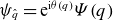 $\psi _{\hat {q}} = \mathrm{e}^{\mathrm{i}\theta (q)}\varPsi (q)$
and derive the envelope operator
$\psi _{\hat {q}} = \mathrm{e}^{\mathrm{i}\theta (q)}\varPsi (q)$
and derive the envelope operator
 $\hat {\mathcal{H}}_{\mathsf{y}}$
for the envelope
$\hat {\mathcal{H}}_{\mathsf{y}}$
for the envelope
 $\varPsi$
in the
$\varPsi$
in the
 $q$
-space the same way the envelope equation was derived in § 4.1 in the
$q$
-space the same way the envelope equation was derived in § 4.1 in the
 $x$
-space. If
$x$
-space. If
 ${\varUpsilon }$
is small globally, i.e. if
${\varUpsilon }$
is small globally, i.e. if
 $H_{\mathsf{z}}$
is mostly linear in
$H_{\mathsf{z}}$
is mostly linear in
 ${\mathsf{z}}$
(locally) at all
${\mathsf{z}}$
(locally) at all
 ${\mathsf{z}}$
, this envelope equation will remain sufficient indefinitely. However, such dispersion operators are rarely found in practice. A typical
${\mathsf{z}}$
, this envelope equation will remain sufficient indefinitely. However, such dispersion operators are rarely found in practice. A typical
 $H_{\mathsf{z}}$
is a nonlinear function of
$H_{\mathsf{z}}$
is a nonlinear function of
 $\mathsf{z}$
, so the choice of the
$\mathsf{z}$
, so the choice of the
 $q$
-representation that is convenient at some
$q$
-representation that is convenient at some
 ${\mathsf{z}}$
is likely to become inconvenient at other
${\mathsf{z}}$
is likely to become inconvenient at other
 ${\mathsf{z}}$
. Then, a single linear transformation is not enough.
${\mathsf{z}}$
. Then, a single linear transformation is not enough.
There are two ways to deal with this problem. One is to define different linear transformations at different points
 ${\mathsf{z}}_0^{(i)}$
along the ray and use MTs to map the wavefield from the
${\mathsf{z}}_0^{(i)}$
along the ray and use MTs to map the wavefield from the
 $q$
-space at
$q$
-space at
 ${\mathsf{z}}_0^{(i)}$
to the
${\mathsf{z}}_0^{(i)}$
to the
 $q$
-space at
$q$
-space at
 ${\mathsf{z}}_0^{(i + 1)}$
(figure 1
a). For example, one can choose
${\mathsf{z}}_0^{(i + 1)}$
(figure 1
a). For example, one can choose
 ${\mathsf{z}}_0^{(i + 1)}$
to be infinitesimally close to
${\mathsf{z}}_0^{(i + 1)}$
to be infinitesimally close to
 ${\mathsf{z}}_0^{(i)}$
; then, the MT for remapping the field will be a near-identity transformation, which can be convenient. This approach is summarised in (Lopez & Dodin Reference Lopez and Dodin2022). The alternative is to use just one but nonlinear transformation such that the new coordinate space is aligned with the ray indefinitely (figure 1
b). No field remapping is needed in this case other than to initialise the field in the new coordinate space and to output the final results back to the
${\mathsf{z}}_0^{(i)}$
; then, the MT for remapping the field will be a near-identity transformation, which can be convenient. This approach is summarised in (Lopez & Dodin Reference Lopez and Dodin2022). The alternative is to use just one but nonlinear transformation such that the new coordinate space is aligned with the ray indefinitely (figure 1
b). No field remapping is needed in this case other than to initialise the field in the new coordinate space and to output the final results back to the
 $x$
-space. This is the approach that we discuss below.
$x$
-space. This is the approach that we discuss below.
Two ways of constructing the
 ${\mathsf{y}}$
-coordinate grids around a reference ray (blue; coincides with the dispersion surface) in the
${\mathsf{y}}$
-coordinate grids around a reference ray (blue; coincides with the dispersion surface) in the
 ${\mathsf{z}}$
-space. (a) Grids are constructed in patches near predefined locations (red dots) on the ray via linear variable transformations. The
${\mathsf{z}}$
-space. (a) Grids are constructed in patches near predefined locations (red dots) on the ray via linear variable transformations. The
 $q$
-axes (red) are tangent to the ray. (b) A single grid is constructed via a nonlinear variable transformation. The coordinate axis (red) coincides with the ray indefinitely.
$q$
-axes (red) are tangent to the ray. (b) A single grid is constructed via a nonlinear variable transformation. The coordinate axis (red) coincides with the ray indefinitely.

5.1.2. Ray path as a coordinate
Let us consider a generic ray that is curved, i.e. has
 $\ddot {{\mathsf{z}}}$
linearly independent from
$\ddot {{\mathsf{z}}}$
linearly independent from
 $\dot {{\mathsf{z}}}$
in the region of interest. (Straight rays can be handled as a limit; see later.) Then, at any given
$\dot {{\mathsf{z}}}$
in the region of interest. (Straight rays can be handled as a limit; see later.) Then, at any given
 ${\mathsf{z}}_0$
on the ray, the vectors
${\mathsf{z}}_0$
on the ray, the vectors
 \begin{gather} {\mathsf{v}} = \dot {{\mathsf{z}}}_0, \quad {\mathsf{u}} = \ddot {{\mathsf{z}}}_0 \end{gather}
form a symplectic basisFootnote 28
 \begin{gather} {\mathsf{s}}_q = {\mathsf{v}}/v, \quad {\mathsf{s}}_p = {\mathsf{u}}/u, \quad {\mathsf{s}}_q \wedge {\mathsf{s}}_p = 1, \end{gather}
where
 $u \doteq {\mathsf{v}} \wedge {\mathsf{u}}/v$
and the scalar
$u \doteq {\mathsf{v}} \wedge {\mathsf{u}}/v$
and the scalar
 $v$
remains to be defined. This basis can be used to construct new ray-aligned coordinates
$v$
remains to be defined. This basis can be used to construct new ray-aligned coordinates
 ${\mathsf{r}} = (\tau , h)$
(here, ‘
${\mathsf{r}} = (\tau , h)$
(here, ‘
 ${\mathsf{r}}$
’ stands for ‘ray’) such that the ray itself would be an isoline of the new momentum
${\mathsf{r}}$
’ stands for ‘ray’) such that the ray itself would be an isoline of the new momentum
 $h$
. Then, one can derive the envelope equation as a partial differential equation (PDE) in the new-coordinate representation. The envelope remains slow in this representation because the reference wavevector satisfies the dispersion relation indefinitely and there are no cutoffs in this representation by construction of
$h$
. Then, one can derive the envelope equation as a partial differential equation (PDE) in the new-coordinate representation. The envelope remains slow in this representation because the reference wavevector satisfies the dispersion relation indefinitely and there are no cutoffs in this representation by construction of
 ${\mathsf{ r}}$
.
${\mathsf{ r}}$
.
Since we are interested only in the local dynamics on the ray, it will be sufficient for us to find
 ${\mathsf{r}}({\mathsf{z}})$
and said PDE near a predefined generic
${\mathsf{r}}({\mathsf{z}})$
and said PDE near a predefined generic
 ${\mathsf{z}}_0$
on the ray. Then, it is convenient to search for the mapping
${\mathsf{z}}_0$
on the ray. Then, it is convenient to search for the mapping
 ${\mathsf{z}} \mapsto {\mathsf{r}}$
as a superposition of two transformations:
${\mathsf{z}} \mapsto {\mathsf{r}}$
as a superposition of two transformations:
 \begin{gather} \underbrace {(x, k)^{\intercal }}_{{\mathsf{z}}} \mapsto \underbrace {(q, p)^{\intercal }}_{{\mathsf{y}}} \mapsto \underbrace {(\tau , h)^{\intercal }}_{\mathsf{r}}. \end{gather}
The first one,
 ${\mathsf{y}} = \bar {{{\mathsf{S}}}} ({\mathsf{z}} - {\mathsf{z}}_0)$
, is the same as in § 5.1.1, except now
${\mathsf{y}} = \bar {{{\mathsf{S}}}} ({\mathsf{z}} - {\mathsf{z}}_0)$
, is the same as in § 5.1.1, except now
 ${\mathsf{ u}}$
is specified by (5.11); i.e. the
${\mathsf{ u}}$
is specified by (5.11); i.e. the
 $q$
-axis is tangent to the ray at
$q$
-axis is tangent to the ray at
 ${\mathsf{z}} = {\mathsf{z}}_0$
. The second transformation,
${\mathsf{z}} = {\mathsf{z}}_0$
. The second transformation,
 ${\mathsf{y}} \mapsto {\mathsf{r}}$
, is nonlinear and modifies the coordinate grid such that the new coordinate axis coincides with the ray. (The momentum axis is also modified accordingly, such that the canonical commutation relation (3.2) is preserved.) The advantage of the splitting (5.13) is that the mapping
${\mathsf{y}} \mapsto {\mathsf{r}}$
, is nonlinear and modifies the coordinate grid such that the new coordinate axis coincides with the ray. (The momentum axis is also modified accordingly, such that the canonical commutation relation (3.2) is preserved.) The advantage of the splitting (5.13) is that the mapping
 ${\mathsf{z}} \mapsto {\mathsf{y}}$
is easy to construct exactly and, for smooth rays,
${\mathsf{z}} \mapsto {\mathsf{y}}$
is easy to construct exactly and, for smooth rays,
 ${\mathsf{y}} \mapsto {\mathsf{ r}}$
can also be found analytically, at least asymptotically. In the following, we show how to do this step by step.
${\mathsf{y}} \mapsto {\mathsf{ r}}$
can also be found analytically, at least asymptotically. In the following, we show how to do this step by step.
5.2. ‘Osculating’ harmonic oscillator
Let us start with a simplified model, where
 $H_{\mathsf{z}}$
can be adequately approximated (locally) with its second-order Taylor expansion in
$H_{\mathsf{z}}$
can be adequately approximated (locally) with its second-order Taylor expansion in
 ${\mathsf{z}} - {\mathsf{z}}_0$
:Footnote
29
${\mathsf{z}} - {\mathsf{z}}_0$
:Footnote
29
 \begin{gather} H_{\mathsf{z}}({\mathsf{z}}) = - ({\mathsf{z}} - {\mathsf{z}}_0) \boldsymbol{\cdot} {\mathsf{J}} {\mathsf{v}} + \frac {1}{2}\,({\mathsf{z}} - {\mathsf{z}}_0) \boldsymbol{\cdot} {\mathsf{g}}({\mathsf{z}} - {\mathsf{z}}_0). \end{gather}
Here,
 ${\mathsf{v}} \doteq {\mathsf{J}} \partial _{\mathsf{z}} H_{\mathsf{z}}({\mathsf{z}}_0) \equiv \dot {{\mathsf{z}}}_0$
, as earlier, and
${\mathsf{v}} \doteq {\mathsf{J}} \partial _{\mathsf{z}} H_{\mathsf{z}}({\mathsf{z}}_0) \equiv \dot {{\mathsf{z}}}_0$
, as earlier, and
 ${\mathsf{g}}$
is a symmetric matrix given by
${\mathsf{g}}$
is a symmetric matrix given by
 ${\mathsf{g}} \doteq (\partial ^2_{\mathsf{z}} H)_0$
. A related description of this model can also be found in Tracy et al. (Reference Tracy, Brizard, Richardson and Kaufman2014, § 5.3.3) for a specific form of
${\mathsf{g}} \doteq (\partial ^2_{\mathsf{z}} H)_0$
. A related description of this model can also be found in Tracy et al. (Reference Tracy, Brizard, Richardson and Kaufman2014, § 5.3.3) for a specific form of
 $H_{\mathsf{z}}$
. Here, we allow for a general
$H_{\mathsf{z}}$
. Here, we allow for a general
 $H_{\mathsf{z}}$
to keep the theory symplectically invariant, at least in its final form discussed in § 5.4.
$H_{\mathsf{z}}$
to keep the theory symplectically invariant, at least in its final form discussed in § 5.4.
Equation (5.14) leads to the following Hamilton’s equations:
 \begin{gather} \dot {{\mathsf{z}}} = {\mathsf{v}} + {\mathsf{J}} {\mathsf{g}}({\mathsf{z}} - {\mathsf{z}}_0), \quad \ddot {{\mathsf{z}}} = {\mathsf{J}} {\mathsf{g}}\dot {{\mathsf{z}}}, \end{gather}
so
 $\ddot {{\mathsf{z}}}_0 = ({\mathsf{J}} {\mathsf{g}}\dot {{\mathsf{z}}})_0 = {\mathsf{J}} {\mathsf{ g}}{\mathsf{v}}$
. Then,
$\ddot {{\mathsf{z}}}_0 = ({\mathsf{J}} {\mathsf{g}}\dot {{\mathsf{z}}})_0 = {\mathsf{J}} {\mathsf{ g}}{\mathsf{v}}$
. Then,
 ${\mathsf{u}} = {\mathsf{J}} {\mathsf{g}}{\mathsf{v}}$
and
${\mathsf{u}} = {\mathsf{J}} {\mathsf{g}}{\mathsf{v}}$
and
 $u = - \varepsilon /v$
. Here,
$u = - \varepsilon /v$
. Here,
 $v$
is a normalisation factor that was introduced in (5.5) and remains to be specified. Also,
$v$
is a normalisation factor that was introduced in (5.5) and remains to be specified. Also,
 \begin{gather} \varepsilon \doteq (\ddot {{\mathsf{z}}} \wedge \dot {{\mathsf{z}}})_0 = ({\mathsf{J}} {\mathsf{g}} {\mathsf{v}})^{\intercal } {\mathsf{J}} {\mathsf{v}} = {\mathsf{v}} \boldsymbol{\cdot} {\mathsf{g}}{\mathsf{v}}, \end{gather}
where we used
 ${\mathsf{J}}^{\intercal }{\mathsf{J}} = {{\mathsf{I}}}$
and
${\mathsf{J}}^{\intercal }{\mathsf{J}} = {{\mathsf{I}}}$
and
 ${\mathsf{ g}}^{\intercal } = {\mathsf{g}}$
. Also note that
${\mathsf{ g}}^{\intercal } = {\mathsf{g}}$
. Also note that
 \begin{align}&\qquad\qquad\quad {\mathsf{v}} \boldsymbol{\cdot} {\mathsf{g}}{\mathsf{u}} = {\mathsf{v}} \boldsymbol{\cdot} {\mathsf{g}} {\mathsf{J}} {\mathsf{g}}{\mathsf{v}} = ({\mathsf{g}}{\mathsf{v}}) \wedge ({\mathsf{g}}{\mathsf{v}}) = 0,\\[-10pt]\nonumber \end{align}
 \begin{align}& {\mathsf{u}} \boldsymbol{\cdot} {\mathsf{g}} {\mathsf{u}} = ({\mathsf{J}} {\mathsf{g}}{\mathsf{v}})^{\intercal } {\mathsf{g}} ({\mathsf{J}} {\mathsf{g}}{\mathsf{v}}) = {\mathsf{v}}^{\intercal } {\mathsf{g}}^{\intercal } {\mathsf{J}}^{\intercal } {\mathsf{g}} {\mathsf{J}} {\mathsf{g}} {\mathsf{v}} = {\mathsf{v}} \boldsymbol{\cdot} {\mathsf{g}} ({-}{\mathsf{J}} {\mathsf{g}} {\mathsf{J}} {\mathsf{g}}) {\mathsf{v}} = g \varepsilon , \end{align}
where we used
 ${\mathsf{J}}^{\intercal } = -{\mathsf{J}}$
, and, for
${\mathsf{J}}^{\intercal } = -{\mathsf{J}}$
, and, for
 $2 \times 2$
matrices,
$2 \times 2$
matrices,
 $-{\mathsf{J}} {\mathsf{g}} {\mathsf{J}} {\mathsf{g}} = g{{\mathsf{I}}}$
, where
$-{\mathsf{J}} {\mathsf{g}} {\mathsf{J}} {\mathsf{g}} = g{{\mathsf{I}}}$
, where
 $g \doteq \det {\mathsf{g}}$
. Similarly, the time derivative of
$g \doteq \det {\mathsf{g}}$
. Similarly, the time derivative of
 $\ddot {{\mathsf{z}}} \wedge \dot {{\mathsf{z}}}$
is
$\ddot {{\mathsf{z}}} \wedge \dot {{\mathsf{z}}}$
is
 \begin{gather} \dddot {{\mathsf{z}}} \wedge \dot {{\mathsf{z}}} = ({\mathsf{J}} {\mathsf{g}} \ddot {{\mathsf{z}}}) \wedge \dot {{\mathsf{z}}} = \ddot {{\mathsf{z}}}^{\intercal } {\mathsf{g}}^{\intercal } {\mathsf{J}}^{\intercal } {\mathsf{J}} \dot {{\mathsf{z}}} = \ddot {{\mathsf{z}}}^{\intercal } {\mathsf{g}} \dot {{\mathsf{z}}} = \ddot {{\mathsf{z}}}^{\intercal } {\mathsf{J}}^{\intercal } ({\mathsf{J}} {\mathsf{g}} \dot {{\mathsf{z}}}) = -\ddot {{\mathsf{z}}} \wedge \ddot {{\mathsf{z}}} = 0, \end{gather}
so
 $\ddot {{\mathsf{z}}} \wedge \dot {{\mathsf{z}}} = (\ddot {{\mathsf{z}}} \wedge \dot {{\mathsf{ z}}})_0$
. This means that, to the extent that the model (5.14) is applicable, one can replace the definition (5.16) with
$\ddot {{\mathsf{z}}} \wedge \dot {{\mathsf{z}}} = (\ddot {{\mathsf{z}}} \wedge \dot {{\mathsf{ z}}})_0$
. This means that, to the extent that the model (5.14) is applicable, one can replace the definition (5.16) with
 $\varepsilon = \ddot {{\mathsf{z}}} \wedge \dot {{\mathsf{z}}}$
.
$\varepsilon = \ddot {{\mathsf{z}}} \wedge \dot {{\mathsf{z}}}$
.
Let us use these results to see how (5.14) is transformed by the mapping
 ${\mathsf{z}} \mapsto {\mathsf{y}}$
. The first term in (5.14) becomes
${\mathsf{z}} \mapsto {\mathsf{y}}$
. The first term in (5.14) becomes
 $p v$
, like before. The second term becomes
$p v$
, like before. The second term becomes
 \begin{align} \frac {1}{2}\,({\mathsf{z}} - {\mathsf{z}}_0) \boldsymbol{\cdot} {\mathsf{g}}({\mathsf{z}} - {\mathsf{z}}_0) & = \frac {1}{2}\,{\mathsf{y}}^{\intercal } \left ( \begin{array}{c} {\mathsf{v}}^{\intercal }/v\\[4pt] {\mathsf{u}}^{\intercal }/u \end{array} \right ) {\mathsf{g}} \left ( \begin{array}{c@{\quad}c} {\mathsf{v}}/v & {\mathsf{u}}/u \end{array} \right ) {\mathsf{y}} \notag \\[4pt] & = \frac {1}{2}\,{\mathsf{y}} \boldsymbol{\cdot} \left ( \begin{array}{c@{\quad}c} {\mathsf{v}} \boldsymbol{\cdot} {\mathsf{g}} {\mathsf{v}}/v^2 & {\mathsf{v}} \boldsymbol{\cdot} {\mathsf{g}} {\mathsf{u}}/vu\\[4pt] {\mathsf{u}} \boldsymbol{\cdot} {\mathsf{g}} {\mathsf{v}}/vu & {\mathsf{u}} \boldsymbol{\cdot} {\mathsf{g}} {\mathsf{u}}/u^2 \end{array} \right ) {\mathsf{y}} \notag \\[4pt] & = \frac {1}{2}\,{\mathsf{y}} \boldsymbol{\cdot} \left ( \begin{array}{c@{\quad}c} \varepsilon /v^2 & 0\\[4pt] 0 & gv^2/\varepsilon \end{array} \right ) {\mathsf{y}}. \end{align}
Assuming the notation
 $\sigma _f \doteq {\textrm {sgn}} f$
for any
$\sigma _f \doteq {\textrm {sgn}} f$
for any
 $f$
, let us introduce
$f$
, let us introduce
 $\varOmega \doteq \sigma _\varepsilon \sqrt {|g|}$
and choose
$\varOmega \doteq \sigma _\varepsilon \sqrt {|g|}$
and choose
 $v = (\varepsilon ^2/|g|)^{1/4}$
, so that the absolute values of the diagonal elements in the matrix in (5.20) are the same. Then,
$v = (\varepsilon ^2/|g|)^{1/4}$
, so that the absolute values of the diagonal elements in the matrix in (5.20) are the same. Then,
 $\varepsilon /v^2 = |g|v^2/\varepsilon = \varOmega$
, so
$\varepsilon /v^2 = |g|v^2/\varepsilon = \varOmega$
, so
 $v = |\varepsilon /\varOmega |^{1/2}$
,
$v = |\varepsilon /\varOmega |^{1/2}$
,
 $u = - \sigma _\varepsilon |\varepsilon \varOmega |^{1/2}$
and
$u = - \sigma _\varepsilon |\varepsilon \varOmega |^{1/2}$
and
 \begin{gather} \left ( \begin{array}{c@{\quad}c} \varepsilon /v^2 & 0\\[4pt] 0 & gv^2/\varepsilon \end{array} \right ) = \varOmega \left ( \begin{array}{c@{\quad}c} 1 & 0\\[2pt] 0 & \sigma _g \end{array} \right )\!. \end{gather}
Then,
 \begin{gather} H_{{\mathsf{y}}}({\mathsf{y}}) = H_{\mathsf{z}}({\mathsf{z}}) = \frac {\varOmega }{2}(q^2 + \sigma _g (p + R)^2 - \sigma _g R^2), \end{gather}
where
 $R \doteq \sigma _g v/\varOmega$
, so
$R \doteq \sigma _g v/\varOmega$
, so
 $|R| = |v/\varOmega | = |\varepsilon |^{1/2}|g|^{-3/4}$
.Footnote
30
One can recognise this procedure as the Williamson diagonalisation of
$|R| = |v/\varOmega | = |\varepsilon |^{1/2}|g|^{-3/4}$
.Footnote
30
One can recognise this procedure as the Williamson diagonalisation of
 ${\mathsf{g}}$
(at least, for
${\mathsf{g}}$
(at least, for
 $g \gt 0$
), with
$g \gt 0$
), with
 $\varOmega$
being the symplectic eigenvalue of
$\varOmega$
being the symplectic eigenvalue of
 ${\mathsf{g}}$
(Nicacio Reference Nicacio2021). Note that
${\mathsf{g}}$
(Nicacio Reference Nicacio2021). Note that
 $\varOmega$
and
$\varOmega$
and
 $R$
are symplectic invariants by definition, and so are
$R$
are symplectic invariants by definition, and so are
 $\varepsilon$
,
$\varepsilon$
,
 $g$
and
$g$
and
 $v$
. Also, it is easily seen that
$v$
. Also, it is easily seen that
 $R$
is dimensionless and the other quantities have the following units (the square brackets here stand for ‘units of ’):
$R$
is dimensionless and the other quantities have the following units (the square brackets here stand for ‘units of ’):
 \begin{gather} [\varepsilon ] = [H_{\mathsf{z}}]^3, \quad [g] = [H_{\mathsf{z}}]^2, \quad [\varOmega ] = [H_{\mathsf{z}}], \quad [v] = [H_{\mathsf{z}}]. \end{gather}
Also useful for us will be the following formula:
 \begin{gather} |\varepsilon |^{1/3} = |\varOmega \| R|^{2/3} = v/|R|^{1/3}. \end{gather}
The phase-space variables
 $(q, p)^{\intercal } \equiv {\mathsf{y}}$
can be understood as a local approximation to the natural canonical variables of
$(q, p)^{\intercal } \equiv {\mathsf{y}}$
can be understood as a local approximation to the natural canonical variables of
 $\hat {H}$
. The matrix
$\hat {H}$
. The matrix
 ${\mathsf{g}}$
serves as a natural (pseudo)metric induced by
${\mathsf{g}}$
serves as a natural (pseudo)metric induced by
 $\hat {H}$
on the symplectic space; then,
$\hat {H}$
on the symplectic space; then,
 $\varepsilon = \|{\mathsf{v}}\|_{\mathsf{g}}^2$
can be understood as the square of
$\varepsilon = \|{\mathsf{v}}\|_{\mathsf{g}}^2$
can be understood as the square of
 ${\mathsf{ v}}$
in this metric. The ray trajectories in the
${\mathsf{ v}}$
in this metric. The ray trajectories in the
 ${\mathsf{y}}$
-space satisfy
${\mathsf{y}}$
-space satisfy
 $H_{{\mathsf{ y}}}({\mathsf{y}}) = 0$
, so, within the approximation (5.22), they are conic sections: circles at
$H_{{\mathsf{ y}}}({\mathsf{y}}) = 0$
, so, within the approximation (5.22), they are conic sections: circles at
 $g \gt 0$
, parabolas at
$g \gt 0$
, parabolas at
 $g = 0$
and hyperbolas at
$g = 0$
and hyperbolas at
 $g \lt 0$
. However, we are interested only in small
$g \lt 0$
. However, we are interested only in small
 $q$
and
$q$
and
 $p$
, in which case
$p$
, in which case
 $\sigma _g$
has little effect on the ray trajectories (figure 2).Footnote
31
Hence, locally, the ray dynamics can be thought of as the dynamics of a harmonic oscillator with the Hamiltonian
$\sigma _g$
has little effect on the ray trajectories (figure 2).Footnote
31
Hence, locally, the ray dynamics can be thought of as the dynamics of a harmonic oscillator with the Hamiltonian
 \begin{gather} H_{{\mathsf{y}}}({\mathsf{y}}) = \frac {\varOmega }{2}\,(q^2 + (p + R)^2 - R^2). \end{gather}
We call it the ‘osculating’ harmonic oscillator (OHO). (To a dynamical system, an OHO basically is what an osculating circle is to a curve.) The phase-space orbit of OHO is a circle with radius
 $|R|$
. Since our approximation (5.14) is generally adequate only on scales small compared with this scale, our model is applicable only when both
$|R|$
. Since our approximation (5.14) is generally adequate only on scales small compared with this scale, our model is applicable only when both
 $q$
and
$q$
and
 $p$
are much less than
$p$
are much less than
 $R$
.
$R$
.
Ray trajectories
 $H_{{\mathsf{y}}}({\mathsf{y}}) = 0$
for various signs of
$H_{{\mathsf{y}}}({\mathsf{y}}) = 0$
for various signs of
 $g$
and
$g$
and
 $\varepsilon$
. Darker colours mark, loosely, the areas of where the assumed model is adequate. Lighter colours mark the areas that are beyond the validity domain of the model. The arrows mark the direction of the ray propagation, which is always towards positive
$\varepsilon$
. Darker colours mark, loosely, the areas of where the assumed model is adequate. Lighter colours mark the areas that are beyond the validity domain of the model. The arrows mark the direction of the ray propagation, which is always towards positive
 $q$
. In the two right columns, dashed are the osculating circles. The radius of each circle is
$q$
. In the two right columns, dashed are the osculating circles. The radius of each circle is
 $|R| = |v/\varOmega |$
. Dotted are the asymptotes of the hyperbolas.
$|R| = |v/\varOmega |$
. Dotted are the asymptotes of the hyperbolas.

The parameter
 $\varOmega$
can be understood as OHO’s angular frequency. At
$\varOmega$
can be understood as OHO’s angular frequency. At
 $\varOmega \gt 0$
, or
$\varOmega \gt 0$
, or
 $\varepsilon \gt 0$
, the phase-space trajectory is oriented clockwise, as usual. (Note that the canonical phase of the oscillator normally grows when the polar angle on the
$\varepsilon \gt 0$
, the phase-space trajectory is oriented clockwise, as usual. (Note that the canonical phase of the oscillator normally grows when the polar angle on the
 $(q, p)$
plane decreases.) At
$(q, p)$
plane decreases.) At
 $\varOmega \lt 0$
, or
$\varOmega \lt 0$
, or
 $\varepsilon \lt 0$
, the trajectory is counter-clockwise. At
$\varepsilon \lt 0$
, the trajectory is counter-clockwise. At
 $\varOmega = 0$
, which corresponds to
$\varOmega = 0$
, which corresponds to
 $\varepsilon = 0$
, the trajectory is flat, i.e.
$\varepsilon = 0$
, the trajectory is flat, i.e.
 $R = \infty$
. Hence, it is convenient to classify the ray trajectories in terms of their (dimensionless) ‘symplectic curvature’
$R = \infty$
. Hence, it is convenient to classify the ray trajectories in terms of their (dimensionless) ‘symplectic curvature’
 \begin{gather} \kappa \doteq \frac {1}{R} = \frac {\varOmega }{v} = \sigma _\varepsilon \,\frac {|g|^{3/4}}{|\varepsilon |^{1/2}}, \end{gather}
and
 $R$
will be called the symplectic radius, accordingly. (Here and further,
$R$
will be called the symplectic radius, accordingly. (Here and further,
 ${\textrm {sgn}} R \equiv {\textrm {sgn}}\, \kappa = \sigma _\varepsilon$
.) Note that the symplectic curvature can be very different from the regular curvature of a trajectory in a metric space. In particular, one can easily show that
${\textrm {sgn}} R \equiv {\textrm {sgn}}\, \kappa = \sigma _\varepsilon$
.) Note that the symplectic curvature can be very different from the regular curvature of a trajectory in a metric space. In particular, one can easily show that
 \begin{gather} \varepsilon = - \frac {{\mathrm{d}}^2 x}{{\mathrm{d}} k^2}\left (\frac {\partial H_{\mathsf{z}}}{\partial x}\right )^3 = - \frac {{\mathrm{d}}^2 k}{{\mathrm{d}} x^2}\left (\frac {\partial H_{\mathsf{z}}}{\partial k}\right )^3, \end{gather}
where the full derivatives are taken along the ray trajectory,
 $H_{{\mathsf{z}}}({\mathsf{z}}) = 0$
. Thus, at inflection points (where
$H_{{\mathsf{z}}}({\mathsf{z}}) = 0$
. Thus, at inflection points (where
 $\varepsilon \to 0$
),
$\varepsilon \to 0$
),
 $\kappa$
is infinite, whereas the regular curvature would be zero.
$\kappa$
is infinite, whereas the regular curvature would be zero.
Finally, notice the following. The OHO approximation (5.25) for
 $H_{\mathsf{z}}$
corresponds to the following approximation of
$H_{\mathsf{z}}$
corresponds to the following approximation of
 $\hat {H}$
itself:
$\hat {H}$
itself:
 $\hat {H} \approx (\varOmega /2)(\hat {q}^2 + (\hat {p} + R)^2 - R^2)$
. This means that, in the absence of dissipation, the wave (4.16) becomes the equation of a quantum harmonic oscillator (QHO) with energy
$\hat {H} \approx (\varOmega /2)(\hat {q}^2 + (\hat {p} + R)^2 - R^2)$
. This means that, in the absence of dissipation, the wave (4.16) becomes the equation of a quantum harmonic oscillator (QHO) with energy
 $\varOmega R^2/2$
, in the natural units that correspond to unit Planck constant,
$\varOmega R^2/2$
, in the natural units that correspond to unit Planck constant,
 $\hbar = 1$
. Since the QHO energy can be expressed through its quantum mode number
$\hbar = 1$
. Since the QHO energy can be expressed through its quantum mode number
 $n$
as
$n$
as
 $\varOmega (n + 1/2)$
, one obtains
$\varOmega (n + 1/2)$
, one obtains
 \begin{gather} n = \frac {R^2}{2} - \frac {1}{2}. \end{gather}
This readily determines applicability conditions for GO in the
 $q$
-representation in the region
$q$
-representation in the region
 $q \ll R$
in which we are interested. Indeed, as commonly known, one can adequately approximate the dynamics of such QHO using GO at
$q \ll R$
in which we are interested. Indeed, as commonly known, one can adequately approximate the dynamics of such QHO using GO at
 $n \gg 1$
, i.e.
$n \gg 1$
, i.e.
 $R \gg 1$
. This makes
$R \gg 1$
. This makes
 $\kappa$
a natural small parameter for MGO. One might be surprised that this parameter becomes infinite at inflection points, where rays become straight and thus, supposedly, MGO should work only better. However, notice that, near inflection points,
$\kappa$
a natural small parameter for MGO. One might be surprised that this parameter becomes infinite at inflection points, where rays become straight and thus, supposedly, MGO should work only better. However, notice that, near inflection points,
 $R$
evolves faster than the ray moves along the OHO trajectory per se and, thus, the very concept of the orbit radius becomes irrelevant. In other words, the quadratic approximation (5.14) is inapplicable in such regimes and one should either include cubic terms or simply ignore the effects produced by the quadratic terms, in which case MGO is reinstated. What matters then is not the local
$R$
evolves faster than the ray moves along the OHO trajectory per se and, thus, the very concept of the orbit radius becomes irrelevant. In other words, the quadratic approximation (5.14) is inapplicable in such regimes and one should either include cubic terms or simply ignore the effects produced by the quadratic terms, in which case MGO is reinstated. What matters then is not the local
 $R$
per se, but the characteristic
$R$
per se, but the characteristic
 $R$
. We will return to this subject in § 5.4.
$R$
. We will return to this subject in § 5.4.
5.3. Parabolic approximation
There is more than one way to define the transformation
 ${\mathsf{y}} \mapsto {\mathsf{r}}$
near a given
${\mathsf{y}} \mapsto {\mathsf{r}}$
near a given
 ${\mathsf{z}}_0$
. One set of obvious variables to try are the angle–action variables of the OHO. However, as discussed in Appendix B, this approach is not optimal, so let us try a different one.
${\mathsf{z}}_0$
. One set of obvious variables to try are the angle–action variables of the OHO. However, as discussed in Appendix B, this approach is not optimal, so let us try a different one.
5.3.1. Operator transformation
As pointed out in § 5.2, the OHO approximation is valid only at
 $q \ll R$
, where
$q \ll R$
, where
 $p \sim q^2/R \ll q$
. Because of this, one can neglect
$p \sim q^2/R \ll q$
. Because of this, one can neglect
 $p^2$
compared with
$p^2$
compared with
 $q^2$
in (5.22) and obtain the following ‘parabolic’ approximation of the ray Hamiltonian:Footnote
32
$q^2$
in (5.22) and obtain the following ‘parabolic’ approximation of the ray Hamiltonian:Footnote
32
 \begin{gather} H_{{\mathsf{y}}}({\mathsf{y}}) = H_{\mathsf{z}}({\mathsf{z}}) \approx pv + \frac {\varOmega }{2}\,q^2. \end{gather}
(Note that this holds for any signs of
 $g$
and
$g$
and
 $\varepsilon$
, so the discontinuous function
$\varepsilon$
, so the discontinuous function
 ${\textrm {sgn}}$
never even appears in this formulation.) Let us now introduce new canonical variables
${\textrm {sgn}}$
never even appears in this formulation.) Let us now introduce new canonical variables
 $(\tau , h)^{\intercal } \equiv {\mathsf{r}}$
such that
$(\tau , h)^{\intercal } \equiv {\mathsf{r}}$
such that
 $h = pv + \varOmega q^2/2$
. To find a suitable
$h = pv + \varOmega q^2/2$
. To find a suitable
 $\tau$
, let us search for the corresponding generating function
$\tau$
, let us search for the corresponding generating function
 $F$
in the type-2 form,
$F$
in the type-2 form,
 $F = F(q, h)$
(Goldstein et al. Reference Goldstein, Poole and Safko2011):
$F = F(q, h)$
(Goldstein et al. Reference Goldstein, Poole and Safko2011):
 \begin{gather} p(q, h) = \partial _q F(q, h), \quad \tau (q, h) = \partial _h F(q, h). \end{gather}
Since
 $p(q, h) = (h - \varOmega q^2/2)/v$
, one has
$p(q, h) = (h - \varOmega q^2/2)/v$
, one has
 $F(q, h) = (h q - \varOmega q^3/6)/v$
(up to an arbitrary function of
$F(q, h) = (h q - \varOmega q^3/6)/v$
(up to an arbitrary function of
 $h$
, which we choose to be zero), so
$h$
, which we choose to be zero), so
 \begin{gather} \tau = q/v, \quad h = pv + \varOmega q^2/2, \end{gather}
where we have repeated the expression for
 $h$
for completeness. Since
$h$
for completeness. Since
 $v$
and
$v$
and
 $w$
are defined as values at a fixed
$w$
are defined as values at a fixed
 ${\mathsf{z}}_0$
, the corresponding operators are given simply by
${\mathsf{z}}_0$
, the corresponding operators are given simply by
 \begin{gather} \hat {\tau } = \hat {q}/v, \quad \hat {h} = \hat {p}v + \varOmega \hat {q}^2/2. \end{gather}
(Basically, (5.32) is just a rescaled and truncated small-
 $p$
approximation of (B4).) One can readily see that they exactly satisfy the canonical commutation relation
$p$
approximation of (B4).) One can readily see that they exactly satisfy the canonical commutation relation
 $[\hat {\tau }, \hat {h}] = \mathrm{i}$
.
$[\hat {\tau }, \hat {h}] = \mathrm{i}$
.
5.3.2. M-waves
In addition to avoiding infinite series, the previous model is advantageous in that it allows one to explicitly calculate
 $M$
-waves in a closed form. Indeed, (3.23) for
$M$
-waves in a closed form. Indeed, (3.23) for ![]() becomes an equation solvable analytically:
becomes an equation solvable analytically:
 \begin{gather} \mathrm{i} \partial _\tau \bar {M} = -\mathrm{i} v \partial _q \bar {M} + \frac {1}{2}\,w q^2 \bar {M} \end{gather}
(and (3.19) is just the complex conjugate thereof). Since
 $\hat {\tau } = \hat {q}/v$
, one can adopt
$\hat {\tau } = \hat {q}/v$
, one can adopt ![]() ; then, the initial condition for (5.33) is
; then, the initial condition for (5.33) is
The corresponding solution of (5.33) is
 \begin{gather} \bar {M}(q, \tau ) = \frac {1}{\sqrt {v}}\,\delta \left (\tau - \frac {q}{v}\right ) \exp \left ({-}\frac {\mathrm{i} \varOmega q^3}{6v}\right )\!. \end{gather}
Accordingly, the pseudo-measure (3.29), with
 $M \equiv \bar {M}^*$
, is given by
$M \equiv \bar {M}^*$
, is given by
 \begin{align} \mu & = \frac {1}{2\pi } \int {\mathrm{d}} s'\,{\mathrm{d}} s\, M(\tau + s/2, q + s'\!/2) \, M^*(\tau - s/2, q - s'\!/2)\,\mathrm{e}^{-\mathrm{i} h s + \mathrm{i} p s'} \notag \\ & = \frac {1}{2\pi v} \int {\mathrm{d}} s\,{\mathrm{d}} s'\, \delta \left (\tau - \frac {q}{v} + \frac {s - s'\!/v}{2}\right ) \delta \left (\tau - \frac {q}{v} - \frac {s - s'\!/v}{2}\right ) \notag \\ & \quad \times \exp \left ( \frac {\mathrm{i} \varOmega }{6v}\left (q + \frac {s'}{2}\right )^3 - \frac {\mathrm{i} \varOmega }{6v}\left (q - \frac {s'}{2}\right )^3 -\mathrm{i} h s + \mathrm{i} p s' \right ) \notag \\ & = \frac {1}{2\pi v} \int {\mathrm{d}} s\,{\mathrm{d}} s'\, \delta \left (\tau - \frac {q}{v}\right ) \delta \left (s - \frac {s'}{v}\right ) \notag \\ & \quad \times \exp \left ( \frac {\mathrm{i} \varOmega }{6v}\left (q + \frac {s'}{2}\right )^3 - \frac {\mathrm{i} \varOmega }{6v}\left (q - \frac {s'}{2}\right )^3 -\mathrm{i} h s + \mathrm{i} p s' \right ) \notag \\ & = \frac {1}{2\pi } \int {\mathrm{d}} s\, \delta \left (\tau - \frac {q}{v}\right ) \notag \\ & \quad \times \exp \left ( \frac {\mathrm{i} \varOmega }{6v}\left (q + \frac {s v}{2}\right )^3 - \frac {\mathrm{i} \varOmega }{6v}\left (q - \frac {s v}{2}\right )^3 + \mathrm{i} s (p v - h) \right ) \notag \\ & = \frac {1}{2\pi } \int {\mathrm{d}} s\, \delta \left (\tau - \frac {q}{v}\right ) \exp \left ( \frac {\mathrm{i} \varepsilon s^3}{24} + \mathrm{i} s (H_{\mathsf{y}}({\mathsf{y}}) - h) \right )\!, \end{align}
where we used
 $\varOmega v^2 = \varepsilon$
. This result can also be expressed as
$\varOmega v^2 = \varepsilon$
. This result can also be expressed as
 \begin{gather} \mu ({\mathsf{r}}, {\mathsf{y}}) = \textrm {Ai}_\varepsilon (H_{\mathsf{y}}({\mathsf{y}}) - h)\,\delta (\tau - q/v), \end{gather}
where we have introduced the following (real) function, with
 $\gamma$
as a real parameter:
$\gamma$
as a real parameter:
 \begin{gather} \textrm {Ai}_\gamma (z) \doteq \frac {1}{2\pi }\int _{-\infty }^{\infty } {\mathrm{d}} t\,\mathrm{e}^{\mathrm{i} z t + \mathrm{i} \gamma t^3/24} = \frac {2}{|\gamma |^{1/3}}\,\textrm {Ai}\left (\frac {2}{|\gamma |^{1/3}}\,\sigma _\gamma z\right )\!. \end{gather}
Here,
 $\sigma _\gamma \doteq {\textrm {sgn}} \gamma$
, and
$\sigma _\gamma \doteq {\textrm {sgn}} \gamma$
, and
 $\textrm {Ai}$
is the Airy function of the first kind. Importantly (Appendix C),
$\textrm {Ai}$
is the Airy function of the first kind. Importantly (Appendix C),
 \begin{gather} \lim _{\gamma \to 0} \textrm {Ai}_\gamma (z) = \delta (z). \end{gather}
As to be seen, the function
 $\textrm {Ai}_\gamma$
, which we will call a rescaled Airy function (RAF), plays a fundamental role in MGO and emerges in multiple contexts.
$\textrm {Ai}_\gamma$
, which we will call a rescaled Airy function (RAF), plays a fundamental role in MGO and emerges in multiple contexts.
5.4. General case
Let us now present a formulation that is not restricted to the quadratic approximation (5.14) and also subsumes the standard WKB approximation (4.27) as a special case.
5.4.1. Operator transformation
Let us start with assuming a generic
 $H_{\mathsf{z}}$
in the form
$H_{\mathsf{z}}$
in the form
 \begin{gather} H_{\mathsf{z}}({\mathsf{z}}) = \mathcal{H}(x/\Delta x, k/\Delta k), \end{gather}
where
 $\Delta x$
and
$\Delta x$
and
 $\Delta k$
are the characteristic scales of the system in
$\Delta k$
are the characteristic scales of the system in
 $x$
and
$x$
and
 $k$
, respectively, and
$k$
, respectively, and
 $\mathcal{H}$
is some function with order-one scales. Consider new dimensionless variables
$\mathcal{H}$
is some function with order-one scales. Consider new dimensionless variables
 \begin{gather} X \doteq R x/\Delta x, \quad K \doteq R k/\Delta k, \end{gather}
where
 $R$
is a dimensionless constant. We require that the transformation
$R$
is a dimensionless constant. We require that the transformation
 ${\mathsf{z}} \mapsto {\mathsf{Z}} \equiv (X, K)^{\intercal }$
be symplectic; then,
${\mathsf{z}} \mapsto {\mathsf{Z}} \equiv (X, K)^{\intercal }$
be symplectic; then,
 $H_{\mathsf{Z}}({\mathsf{Z}}) = H_{\mathsf{z}}({\mathsf{z}})$
and
$H_{\mathsf{Z}}({\mathsf{Z}}) = H_{\mathsf{z}}({\mathsf{z}})$
and
 \begin{gather} R = \sqrt {\Delta x \Delta k}. \end{gather}
We will call this quantity a symplectic scale. To the extent that the quadratic approximation (5.14) is adequate at least locally,
 $R$
coincides with the absolute value of the symplectic radius that was introduced in § 5.2. For this reason, in the following, we occasionally mix the terms ‘symplectic scale’ and ‘symplectic radius’, and also refer to the inverse symplectic scale as symplectic curvature.
$R$
coincides with the absolute value of the symplectic radius that was introduced in § 5.2. For this reason, in the following, we occasionally mix the terms ‘symplectic scale’ and ‘symplectic radius’, and also refer to the inverse symplectic scale as symplectic curvature.
Much like in § 4.1, our goal now is to derive field equations that are accurate to the first (not zeroth) order in the ‘MGO parameter’
 \begin{gather} \epsilon \doteq R^{-2} \equiv (\Delta x \Delta k)^{-1} \ll 1. \end{gather}
It is similar to the GO parameter introduced in § 4.1, but the absolute value of
 $k$
is now replaced with the spectral-inhomogeneity scale
$k$
is now replaced with the spectral-inhomogeneity scale
 $\Delta k$
; i.e. the smallness of the local wavelength per se is irrelevant. To the extent that the OHO model is applicable,
$\Delta k$
; i.e. the smallness of the local wavelength per se is irrelevant. To the extent that the OHO model is applicable,
 $\epsilon$
coincides with
$\epsilon$
coincides with
 $\kappa ^2$
, where
$\kappa ^2$
, where
 $\kappa$
is the symplectic curvature introduced in § 5.2.
$\kappa$
is the symplectic curvature introduced in § 5.2.
Let us perform a linear canonical transformation
 ${\mathsf{Z}} \mapsto {\mathsf{y}} \equiv (q, p)^{\intercal }$
, as in § 5.1.1, so that the
${\mathsf{Z}} \mapsto {\mathsf{y}} \equiv (q, p)^{\intercal }$
, as in § 5.1.1, so that the
 $q$
-axis is along
$q$
-axis is along
 ${\mathsf{v}}$
that is tangent to the ray. Then,
${\mathsf{v}}$
that is tangent to the ray. Then,
 $H_{\mathsf{ y}}({\mathsf{y}}) = \mathcal{H}(q/R, p/R)$
, so the ray trajectory satisfies
$H_{\mathsf{ y}}({\mathsf{y}}) = \mathcal{H}(q/R, p/R)$
, so the ray trajectory satisfies
 $\mathcal{H}(q/R, p/R) = 0$
. Its solution (for a given branch) can be written in the form
$\mathcal{H}(q/R, p/R) = 0$
. Its solution (for a given branch) can be written in the form
 $p = R\mathcal{P}(q/R) \equiv p(q)$
, where
$p = R\mathcal{P}(q/R) \equiv p(q)$
, where
 $\mathcal{P}$
is an order-one function that has order-one scales. (If
$\mathcal{P}$
is an order-one function that has order-one scales. (If
 $H_{\mathsf{z}}$
is linear in
$H_{\mathsf{z}}$
is linear in
 ${\mathsf{z}}$
, then
${\mathsf{z}}$
, then
 $\mathcal{P} = 0$
by construction. If
$\mathcal{P} = 0$
by construction. If
 $H_{\mathsf{z}}$
is quadratic, then
$H_{\mathsf{z}}$
is quadratic, then
 $p(q) = -R + \sqrt {R^2 - q^2}$
, so
$p(q) = -R + \sqrt {R^2 - q^2}$
, so
 $p(q) \approx q^2/2R$
at
$p(q) \approx q^2/2R$
at
 $q \ll R$
, as in § 5.3.) By Taylor-expanding
$q \ll R$
, as in § 5.3.) By Taylor-expanding
 $H_{\mathsf{ y}}({\mathsf{ y}})$
in
$H_{\mathsf{ y}}({\mathsf{ y}})$
in
 $p - p(q)$
, one obtains
$p - p(q)$
, one obtains
 \begin{gather} H_{\mathsf{y}}({\mathsf{y}}) \approx V(q)(p - p(q)), \end{gather}
where
 $V(q) \doteq (\partial _p H_{\mathsf{y}})_{p = p(q)}$
, so
$V(q) \doteq (\partial _p H_{\mathsf{y}})_{p = p(q)}$
, so
 $V(0) = v$
. Like (4.17), (5.44) can be understood as Hayes’s representation of
$V(0) = v$
. Like (4.17), (5.44) can be understood as Hayes’s representation of
 $H_{\mathsf{y}}$
. For GO, this representation is precise in that it leads to the correct ray equations and correctly captures the leading-order amplitude dynamics, because those are entirely determined by the first-order derivatives of the symbol. The MT that follows from (5.44) will not be exact, because
$H_{\mathsf{y}}$
. For GO, this representation is precise in that it leads to the correct ray equations and correctly captures the leading-order amplitude dynamics, because those are entirely determined by the first-order derivatives of the symbol. The MT that follows from (5.44) will not be exact, because
 ${\mathcal{O}}([p - p(q)]^2)$
terms have been neglected. Still, assuming
${\mathcal{O}}([p - p(q)]^2)$
terms have been neglected. Still, assuming
 $p - p(q) = {\mathcal{O}}(q^2)$
, (5.44) differs from the exact
$p - p(q) = {\mathcal{O}}(q^2)$
, (5.44) differs from the exact
 $H_{\mathsf{y}}$
by at most
$H_{\mathsf{y}}$
by at most
 ${\mathcal{O}}(q^4)$
, which is assumed negligible (at not-too-large
${\mathcal{O}}(q^4)$
, which is assumed negligible (at not-too-large
 $q$
that we are interested in locally).
$q$
that we are interested in locally).
Let us perform a canonical transformation
 ${\mathsf{y}} \,{\mapsto}\, {\mathsf{r}} \equiv (\tau , h)^{\intercal }$
such that
${\mathsf{y}} \,{\mapsto}\, {\mathsf{r}} \equiv (\tau , h)^{\intercal }$
such that
 $h = H_{\mathsf{y}}$
, i.e.Footnote
33
$h = H_{\mathsf{y}}$
, i.e.Footnote
33
 \begin{gather} p(q, h) = p(q) + h/V(q). \end{gather}
Like in § 5.3, to find what the new coordinate
 $\tau$
should be to keep the transformation canonical, we look for a generating function
$\tau$
should be to keep the transformation canonical, we look for a generating function
 $F$
in the type-2 form:
$F$
in the type-2 form:
 \begin{gather} p(q, h) = \partial _q F(q, h), \quad \tau (q, h) = \partial _h F(q, h). \end{gather}
The former gives
 \begin{gather} F(q, h) = \int ^{q}_0 p(\tilde {q}, h)\,{\mathrm{d}} \tilde {q}, \end{gather}
where we set the integration constant to zero by choice. (The tilde is used to distinguish the dummy integration variable
 $\tilde {q}$
from the actual canonical coordinate
$\tilde {q}$
from the actual canonical coordinate
 $q$
.) Then,
$q$
.) Then,
 \begin{gather} \tau (q, h) = \int ^{q}_0 \frac {\partial p(\tilde {q}, h)}{\partial h}\,{\mathrm{d}} \tilde {q} = \int ^{q}_0 \frac {{\mathrm{d}} \tilde {q}}{V(\tilde {q})} \equiv \tau (q). \end{gather}
In other words,
 $\tau$
and
$\tau$
and
 $h$
are the ray time and the ray energy. (By the ray energy, we mean the value of the ray Hamiltonian, not the wave energy that depends on the wave amplitude.) The corresponding operators are
$h$
are the ray time and the ray energy. (By the ray energy, we mean the value of the ray Hamiltonian, not the wave energy that depends on the wave amplitude.) The corresponding operators are
 \begin{gather} \hat {\tau } = \tau (\hat {q}), \quad \hat {h} = \frac {1}{2}(\hat {V} \hat {p} + \hat {p} \hat {V}) - \hat {V} p(\hat {q}), \end{gather}
where
 $\hat {V} \doteq V(\hat {q})$
(note, though, that
$\hat {V} \doteq V(\hat {q})$
(note, though, that
 $\hat {p}$
is not the same as
$\hat {p}$
is not the same as
 $p(\hat {q})$
), so
$p(\hat {q})$
), so
 $[\hat {\tau }, \hat {V}] = 0$
and
$[\hat {\tau }, \hat {V}] = 0$
and
 \begin{align} [\hat {\tau }, \hat {h}] & = [\hat {\tau }, \hat {V} \hat {p} + \hat {p} \hat {V}]/2 \notag \\ & = (\hat {\tau }\hat {V} \hat {p} - \hat {V} \hat {p}\hat {\tau } + \hat {\tau } \hat {p} \hat {V} - \hat {p} \hat {V} \hat {\tau })/2 \notag \\ & = (\hat {\tau }\hat {V} \hat {p} - \hat {V} [\hat {p}, \hat {\tau }] - \hat {V}\hat {\tau } \hat {p} + \hat {\tau } [\hat {p}, \hat {V}] + \hat {\tau } \hat {V} \hat {p} - \hat {p} \hat {V} \hat {\tau })/2 \notag \\ & = ([\hat {\tau }\hat {V}, \hat {p}] - \hat {V} [\hat {p}, \hat {\tau }] + \hat {\tau } [\hat {p}, \hat {V}])/2 \notag \\ & = \mathrm{i}((\tau (q) V(q))' + V(q) \tau '(q) - \tau (q) V'(q))/2 \notag \\ & = \mathrm{i} V(q)\tau '(q) \notag \\ & = \mathrm{i}. \end{align}
5.4.2. M-waves
The approximation (5.44) corresponds to the following approximation of the operator
 $\hat {H}_{\hat {q}}$
(cf. § 4.1):
$\hat {H}_{\hat {q}}$
(cf. § 4.1):
 \begin{gather} \hat {H}_{\hat {q}} \approx -\mathrm{i} V(q) \partial _q - \frac {\mathrm{i}}{2}\,V'(q) - V(q)p(q). \end{gather}
Then, (3.22) and (3.23) lead to the following equations for
 $\bar {M} \equiv \bar {M}(q, \tau )$
:
$\bar {M} \equiv \bar {M}(q, \tau )$
:
 \begin{align}&\qquad\qquad\qquad (\tau - \tau (q))\bar {M} = 0,\\[-10pt]\nonumber \end{align}
 \begin{align}& \mathrm{i} \partial _\tau \bar {M} = \left ({-}\mathrm{i} V(q) \partial _q - \frac {\mathrm{i}}{2}\,V'(q) - V(q)p(q)\right )\bar {M}. \end{align}
These can be readily solved:
 \begin{gather} \bar {M}(q, \tau ) = \frac {\mathrm{e}^{\mathrm{i} \vartheta (q)}}{\sqrt {V(q)}}\,\delta (\tau - \tau (q)), \quad \vartheta (q) \doteq \int ^{q}_0 p(\tilde {q})\,{\mathrm{d}} \tilde {q}, \end{gather}
which generalises (5.35) to non-constant
 $V(q)$
and arbitrary
$V(q)$
and arbitrary
 $p(q)$
. To the extent that (5.44) is valid, this result is exact. One can also notice parallels with (4.24), which is the same formula applied to different coordinates.
$p(q)$
. To the extent that (5.44) is valid, this result is exact. One can also notice parallels with (4.24), which is the same formula applied to different coordinates.
To calculate the generalisation of the pseudo-measure (5.37), notice that
 \begin{gather} \tau \left (q \pm \frac {s'}{2}\right ) \approx \tau (q) \pm \frac {s'}{2V} - \frac {V'}{8V^2}\,s'^2, \end{gather}
where
 $V \equiv V(q)$
and
$V \equiv V(q)$
and
 $V'(q) \equiv {\mathrm{d}} V(q)/{\mathrm{d}} q$
, while the prime in
$V'(q) \equiv {\mathrm{d}} V(q)/{\mathrm{d}} q$
, while the prime in
 $s'$
is only a notation that distinguishes said variable from
$s'$
is only a notation that distinguishes said variable from
 $s$
. Then,
$s$
. Then,
 \begin{align} & \delta \left ( \tau + \frac {s}{2} - \tau \left (q + \frac {s'}{2}\right ) \right ) \delta \left ( \tau - \frac {s}{2} - \tau \left (q - \frac {s'}{2}\right ) \right ) \notag \\[2pt] & \quad \approx \delta \left ( \tau - \tau (q) + \frac {s - s'\!/V}{2} + \frac {V'{s}^{\prime 2}}{8V^2} \right ) \delta \left ( \tau - \tau (q) - \frac {s - s'\!/V}{2} + \frac {V'{s}^{\prime 2}}{8V^2} \right ) \notag \\[2pt] & \quad = \delta \left (\tau - \tau (q) + \frac {V'{s}^{\prime 2}}{8V^2}\right ) \delta \left (s - \frac {s'}{V}\right ) \notag \\[2pt] & \quad = \delta \left (\tau - \tau (q) + \frac {V's^2}{8}\right ) \delta \left (s - \frac {s'}{V}\right ) \notag \\[2pt] & \quad \approx \left (1 + \frac {V's^2}{8}\,\frac {\partial }{\partial \tau }\right ) \delta (\tau - \tau (q)) \delta \left (s - \frac {s'}{V}\right )\!, \end{align}
where the last equality is based on the first-order Taylor expansion. (Admittedly, Taylor-expanding a delta function is a questionable procedure, but it makes sense as a shorthand for Taylor-expanding what actually matters, namely, integrals of delta functions.) Then,
 \begin{gather} \mu = \big [1 - (V'/8)\,\partial ^3_{\tau h h}\big ]\mu _0, \quad \mu _0 = \mathfrak{A}\, \delta (\tau (q) - \tau ), \end{gather}
where
 $\mathfrak{A}$
is a generalisation of (5.38):
$\mathfrak{A}$
is a generalisation of (5.38):
 \begin{gather} \mathfrak{A} \doteq \frac {1}{2\pi } \int {\mathrm{d}} s\,\mathrm{e}^{\mathrm{i}\varPhi }, \quad \varPhi \doteq (p V - h) s - \int _{q - s V/2}^{q + s V/2} p(\tilde {q})\,{\mathrm{d}}\tilde {q}. \end{gather}
Remember that
 $p$
is an independent variable,
$p$
is an independent variable,
 $V \equiv V(q)$
and
$V \equiv V(q)$
and
 $p(q)$
is a function introduced in § 5.4.1.
$p(q)$
is a function introduced in § 5.4.1.
5.4.3. Symplectically invariant model for
 $\mu$
$\mu$

Since we are already neglecting terms of order
 $V''$
, the factor
$V''$
, the factor
 $V'$
in (5.57) can be considered commuting with the derivatives. Then, using (3.41) and integrating by parts, one obtains the following formula for remapping symbols between the
$V'$
in (5.57) can be considered commuting with the derivatives. Then, using (3.41) and integrating by parts, one obtains the following formula for remapping symbols between the
 ${\mathsf{y}}$
- and
${\mathsf{y}}$
- and
 ${\mathsf{r}}$
- representations:
${\mathsf{r}}$
- representations:
 \begin{gather} O_{\mathsf{y}}({\mathsf{y}}) = \int \left (O_{\mathsf{r}}({\mathsf{r}}) + \frac {V'}{8} \,\partial ^3_{\tau h h} O_{\mathsf{r}}({\mathsf{ r}}) \right )\mu _0 \,{\mathrm{d}}\tau \,{\mathrm{d}} h. \end{gather}
In the following, we will be interested in
 $O_{\mathsf{r}}$
that are either
$O_{\mathsf{r}}$
that are either
 $\tau$
-independent or smooth, namely, have symplectic scales of order
$\tau$
-independent or smooth, namely, have symplectic scales of order
 $R$
or larger. In either case, the second term in (5.59) is
$R$
or larger. In either case, the second term in (5.59) is
 ${\mathcal{O}}(R^{-4})$
, i.e.
${\mathcal{O}}(R^{-4})$
, i.e.
 ${\mathcal{O}}(\epsilon ^2)$
, which is considered negligible. Thus, in the following, we adopt
${\mathcal{O}}(\epsilon ^2)$
, which is considered negligible. Thus, in the following, we adopt
 $\mu \approx \mu _0$
, i.e.
$\mu \approx \mu _0$
, i.e.
 \begin{gather} \mu \approx \mathfrak{A}\, \delta (\tau (q) - \tau ). \end{gather}
One can also show (Appendix C) that, at
 $R \gg 1$
, one can approximate
$R \gg 1$
, one can approximate
 $\mathfrak{A}$
as
$\mathfrak{A}$
as
 \begin{gather} \mathfrak{A} \approx \textrm {Ai}_\varepsilon (H_{\mathsf{y}}({\mathsf{y}}) - h) \end{gather}
with
 $\varepsilon = - V^3 p''$
. In fact, even when (5.43) is not satisfied, yet all higher-order derivatives of
$\varepsilon = - V^3 p''$
. In fact, even when (5.43) is not satisfied, yet all higher-order derivatives of
 $p(q)$
are small enough,
$p(q)$
are small enough,
 $\mathfrak{A}$
can still be approximated with a delta function,
$\mathfrak{A}$
can still be approximated with a delta function,
 $\mathfrak{A} \approx \delta (H_{\mathsf{y}}({\mathsf{y}}) - h)$
, which may be sufficiently accurate for practical purposes. In this case,
$\mathfrak{A} \approx \delta (H_{\mathsf{y}}({\mathsf{y}}) - h)$
, which may be sufficiently accurate for practical purposes. In this case,
 $\mathfrak{A}$
can be safely replaced with
$\mathfrak{A}$
can be safely replaced with
 $\textrm {Ai}_\varepsilon$
because the latter can be approximated with a delta function as well. Hence, we will assume (5.61) either literally, when (5.43) is satisfied, or in the sense that both
$\textrm {Ai}_\varepsilon$
because the latter can be approximated with a delta function as well. Hence, we will assume (5.61) either literally, when (5.43) is satisfied, or in the sense that both
 $\mathfrak{A}$
and
$\mathfrak{A}$
and
 $\textrm {Ai}_\varepsilon$
are close enough to
$\textrm {Ai}_\varepsilon$
are close enough to
 $\delta (H_{\mathsf{y}}({\mathsf{y}}) - h)$
. Then, (5.60) becomes
$\delta (H_{\mathsf{y}}({\mathsf{y}}) - h)$
. Then, (5.60) becomes
 \begin{gather} \mu \approx \textrm {Ai}_\varepsilon (H_{\mathsf{y}}({\mathsf{y}}) - h)\, \delta (\tau (q) - \tau ). \end{gather}
Because
 ${\mathsf{y}}$
and
${\mathsf{y}}$
and
 ${\mathsf{z}}$
are connected by a linear transformation, which preserves
${\mathsf{z}}$
are connected by a linear transformation, which preserves
 $\mu$
, one can also consider (5.62) as the symplectic measure for the whole transformation
$\mu$
, one can also consider (5.62) as the symplectic measure for the whole transformation
 ${\mathsf{r}} \leftrightarrow {\mathsf{z}}$
:
${\mathsf{r}} \leftrightarrow {\mathsf{z}}$
:
 \begin{gather} \mu = \textrm {Ai}_\varepsilon (H_{\mathsf{z}}({\mathsf{z}}) - h)\,\delta (\tau ({\mathsf{z}}) - \tau ). \end{gather}
At
 $\varepsilon \to 0$
, when the transformation
$\varepsilon \to 0$
, when the transformation
 ${\mathsf{z}} \mapsto {\mathsf{r}}$
is linear,Footnote
34
(5.63) yields
${\mathsf{z}} \mapsto {\mathsf{r}}$
is linear,Footnote
34
(5.63) yields
 $\mu ({\mathsf{r}}, {\mathsf{z}}) = \delta (H_{\mathsf{z}}({\mathsf{z}}) - h)\,\delta (\tau ({\mathsf{z}}) - \tau )$
, in agreement with (3.57). Application of (5.63) in the general case requires that one expresses
$\mu ({\mathsf{r}}, {\mathsf{z}}) = \delta (H_{\mathsf{z}}({\mathsf{z}}) - h)\,\delta (\tau ({\mathsf{z}}) - \tau )$
, in agreement with (3.57). Application of (5.63) in the general case requires that one expresses
 $\varepsilon$
as a function of
$\varepsilon$
as a function of
 ${\mathsf{z}}$
(as opposed to
${\mathsf{z}}$
(as opposed to
 $q$
). Since our calculation is valid only for small
$q$
). Since our calculation is valid only for small
 $q$
, multiple coordinate charts would have to be introduced and properly merged for this, which is inconvenient. However, as long as
$q$
, multiple coordinate charts would have to be introduced and properly merged for this, which is inconvenient. However, as long as
 $\varepsilon$
is smooth (or indistinguishable from zero), one can use (5.16) to extrapolate it to all
$\varepsilon$
is smooth (or indistinguishable from zero), one can use (5.16) to extrapolate it to all
 ${\mathsf{z}}$
via
${\mathsf{z}}$
via
 \begin{gather} \varepsilon = ({\mathsf{J}} \partial _{\mathsf{z}} H_{\mathsf{z}}) \boldsymbol{\cdot} (\partial _{\mathsf{z}}^2 H_{\mathsf{ z}}) ({\mathsf{J}} \partial _{\mathsf{z}} H_{\mathsf{z}}). \end{gather}
This ensures that
 $\varepsilon$
is close to the desired value
$\varepsilon$
is close to the desired value
 $\varepsilon = - V^3 p''$
in the ray vicinity, while far from the ray, our result is not expected to be applicable in any case. Then, one can readily transform the symbols of operators with
$\varepsilon = - V^3 p''$
in the ray vicinity, while far from the ray, our result is not expected to be applicable in any case. Then, one can readily transform the symbols of operators with
 \begin{gather} O_{\mathsf{z}}({\mathsf{z}}) \approx \int \textrm {Ai}_\varepsilon (H_{\mathsf{z}}({\mathsf{z}}) - \tilde {h})\,O_{\mathsf{r}}(\tau ({\mathsf{z}}), \tilde {h})\, {\mathrm{d}} \tilde {h}, \end{gather}
i.e.
 $O_{\mathsf{z}}({\mathsf{z}})$
is the Airy transform (Widder Reference Widder1979) of
$O_{\mathsf{z}}({\mathsf{z}})$
is the Airy transform (Widder Reference Widder1979) of
 $O_{\mathsf{r}}$
. Equation (5.65) is one of the key new results of this paper. As will be seen in the following, it is an important theorem that makes MGO a practical theory.
$O_{\mathsf{r}}$
. Equation (5.65) is one of the key new results of this paper. As will be seen in the following, it is an important theorem that makes MGO a practical theory.
Assuming the symplectic scale of
 $O_{\mathsf{r}}$
is of order
$O_{\mathsf{r}}$
is of order
 $R$
, one can take this integral using (C2). This leads to
$R$
, one can take this integral using (C2). This leads to
 $O_{\mathsf{z}}({\mathsf{z}}) \approx O_{\mathsf{r}}(\tau ({\mathsf{z}}), H_{\mathsf{z}}({\mathsf{ z}})) + {\mathcal{O}}(\varepsilon \partial _h^3 O_{\mathsf{r}})$
. Based on (5.64), the second term on the right-hand side can be estimated as
$O_{\mathsf{z}}({\mathsf{z}}) \approx O_{\mathsf{r}}(\tau ({\mathsf{z}}), H_{\mathsf{z}}({\mathsf{ z}})) + {\mathcal{O}}(\varepsilon \partial _h^3 O_{\mathsf{r}})$
. Based on (5.64), the second term on the right-hand side can be estimated as
 $\varepsilon \partial _h^3 O_{\mathsf{r}} \sim O_{\mathsf{r}}/R^4$
. Thus,
$\varepsilon \partial _h^3 O_{\mathsf{r}} \sim O_{\mathsf{r}}/R^4$
. Thus,
 \begin{gather} O_{\mathsf{z}}({\mathsf{z}}) = O_{\mathsf{r}}({\mathsf{r}}({\mathsf{z}})) + {\mathcal{O}}(\epsilon ^2). \end{gather}
The importance of this result is in that the approximate equality
 $O_{\mathsf{z}}({\mathsf{z}}) \approx O_{\mathsf{r}}({\mathsf{r}}({\mathsf{z}}))$
is satisfied with accuracy not
$O_{\mathsf{z}}({\mathsf{z}}) \approx O_{\mathsf{r}}({\mathsf{r}}({\mathsf{z}}))$
is satisfied with accuracy not
 $\mathcal{O}(\epsilon )$
but
$\mathcal{O}(\epsilon )$
but
 ${\mathcal{O}}(\epsilon ^2)$
, which will be negligible for our purposes (§ 6). This is another new key result of this paper.Footnote
35
Keep in mind, though, that (5.66) is invalid for small-scale symbols, such as the delta-shaped symbols discussed in § 6.2. In that case, the more general (5.65) should be used instead.
${\mathcal{O}}(\epsilon ^2)$
, which will be negligible for our purposes (§ 6). This is another new key result of this paper.Footnote
35
Keep in mind, though, that (5.66) is invalid for small-scale symbols, such as the delta-shaped symbols discussed in § 6.2. In that case, the more general (5.65) should be used instead.
6. MGO for scalar waves
6.1. Dynamics in the
$\tau$
-space

Armed with (5.66), we are now ready to formulate the MGO envelope equation. Let us return to our original wave equation (4.16), which accounts for dissipation, and rewrite it in the
 $\tau$
-representation:
$\tau$
-representation:
 \begin{gather} \big(\hat {H}_{\hat {\tau }} + \mathrm{i}\hat {\varGamma }_{\hat {\tau }}\big)\psi _{\hat {\tau }} = 0. \end{gather}
(As earlier, we assume that
 $\psi _{\hat {\tau }}$
is a scalar function, but see § 7.2 for a more general case.) Since
$\psi _{\hat {\tau }}$
is a scalar function, but see § 7.2 for a more general case.) Since
 $\hat {H}_{\hat {\tau }} = \hat {h}_{\hat {\tau }} = -\mathrm{i} \partial _\tau$
, this leads to
$\hat {H}_{\hat {\tau }} = \hat {h}_{\hat {\tau }} = -\mathrm{i} \partial _\tau$
, this leads to
 \begin{gather} \big({-} \partial _\tau + \hat {\varGamma }_{\hat {\tau }}\big)\psi _{\hat {\tau }} = 0. \end{gather}
Assuming that
 $\varGamma _{\mathsf{r}} = {\mathcal{O}}(\epsilon )$
, the operator
$\varGamma _{\mathsf{r}} = {\mathcal{O}}(\epsilon )$
, the operator
 $\hat {\varGamma }_{\hat {\tau }}$
can be approximated simply by its symbol on the reference ray,
$\hat {\varGamma }_{\hat {\tau }}$
can be approximated simply by its symbol on the reference ray,
 $\varGamma _{\mathsf{r}}(\tau )$
. Then, (6.2) becomes
$\varGamma _{\mathsf{r}}(\tau )$
. Then, (6.2) becomes
 \begin{gather} \partial _\tau \psi _{\hat {\tau }} = \varGamma _{\mathsf{r}}(\tau ) \psi _{\hat {\tau }}. \end{gather}
Assuming that
 $\varGamma _{\mathsf{r}}$
is sufficiently smooth, (5.66) predicts that
$\varGamma _{\mathsf{r}}$
is sufficiently smooth, (5.66) predicts that
 $\varGamma _{\mathsf{r}}({\mathsf{r}}) \approx \varGamma _{\mathsf{z}}({\mathsf{z}}({\mathsf{r}}))$
, which is a known function when the dispersion operator is given. Then, (6.3) can be readily integrated,
$\varGamma _{\mathsf{r}}({\mathsf{r}}) \approx \varGamma _{\mathsf{z}}({\mathsf{z}}({\mathsf{r}}))$
, which is a known function when the dispersion operator is given. Then, (6.3) can be readily integrated,
 \begin{gather} \psi _{\hat {\tau }} = a \exp \left (\int {\mathrm{d}}\tau \varGamma _{\mathsf{r}}(\tau )\right )\!, \quad a = \text{const.}, \end{gather}
and, unlike in the GO (4.12), this solution exhibits no singularities. Also notably, the ray equations in the
 ${\mathsf{ r}}$
-representation are particularly simple:
${\mathsf{ r}}$
-representation are particularly simple:
 \begin{gather} \dot {\tau } = 1, \quad \dot {h} = 0. \end{gather}
A generalisation to vector waves is discussed in § 7. One can also generalise the MGO envelope equation to quasioptical beams that experience transverse diffraction. This can be done similarly to how quasioptical equations were derived by Dodin et al. (Reference Dodin, Ruiz, Yanagihara, Zhou and Kubo2019) and Yanagihara, Dodin & Kubo (Reference Yanagihara, Dodin and Kubo2019a , Reference Yanagihara, Dodin and Kubob ) for conventional GO. However, presenting these calculations in detail would require introducing additional cumbersome machinery that is not specific to MGO, so we postpone discussing this subject until further publications.
6.2. Mapping solutions to the
$x$
-space

Mapping solutions to the
 $x$
-space is generally the most challenging part in MGO applications (Donnelly et al. Reference Donnelly, Lopez and Dodin2021; Højlund Marholt et al. Reference Højlund Marholt, Senstius and Nielsen2024; Lopez, Højlund & Senstius Reference Lopez, Højlund and Senstius2024). However, knowing the field at all
$x$
-space is generally the most challenging part in MGO applications (Donnelly et al. Reference Donnelly, Lopez and Dodin2021; Højlund Marholt et al. Reference Højlund Marholt, Senstius and Nielsen2024; Lopez, Højlund & Senstius Reference Lopez, Højlund and Senstius2024). However, knowing the field at all
 $x$
is usually unnecessary. One might not even need to leave the
$x$
is usually unnecessary. One might not even need to leave the
 $\tau$
-space except for initialising the field and also calculating the final state, and those mappings may be easy to do.Footnote
36
In other cases, one can proceed as follows.
$\tau$
-space except for initialising the field and also calculating the final state, and those mappings may be easy to do.Footnote
36
In other cases, one can proceed as follows.
6.2.1. General case
To calculate how the wave evolves in the original
 $x$
-space, one needs to remap the
$x$
-space, one needs to remap the
 $\tau$
-representation to the
$\tau$
-representation to the
 $x$
-representation:
$x$
-representation:
Since ![]() this leads to
this leads to

where
 $\vartheta (q) = \int ^{q}_0 p(\tilde {q})\,{\mathrm{d}} \tilde {q}$
. Since
$\vartheta (q) = \int ^{q}_0 p(\tilde {q})\,{\mathrm{d}} \tilde {q}$
. Since ![]() consists of a phase-space shift (§ 3.5.1) and an LST (§ 3.5.3), the integrand in (6.7) is easy to write explicitly in any given case.
consists of a phase-space shift (§ 3.5.1) and an LST (§ 3.5.3), the integrand in (6.7) is easy to write explicitly in any given case.
How to approximate such an integral depends on the problem and can be done using various techniques, with accuracy requirements determined by specific applications. For example, stationary-phase or steepest-descent methods might suffice, or one might be able to reduce (6.7) to a known representation of a special function. In particular, to the extent that (6.7) can be expressed through the Airy function (or, equivalently, Bessel functions of order
 $1/3$
), it is similar to previous results (Langer Reference Langer1937; Chester, Friedman & Ursell Reference Chester, Friedman and Ursell1957). Similar integrals have been studied also in the context of semiclassical calculations in atomic and molecular physics; for example, see Kay (Reference Kay1994b
).
$1/3$
), it is similar to previous results (Langer Reference Langer1937; Chester, Friedman & Ursell Reference Chester, Friedman and Ursell1957). Similar integrals have been studied also in the context of semiclassical calculations in atomic and molecular physics; for example, see Kay (Reference Kay1994b
).
Remember also that the above-mentioned result is derived under the assumption that only small values of
 $q$
contribute to the integral (6.7). This allows one to derive local approximations
$q$
contribute to the integral (6.7). This allows one to derive local approximations
 $\psi _{\hat {x}}$
using different definitions of
$\psi _{\hat {x}}$
using different definitions of
 $(q, p)$
for different regions of interest. A global representation is not necessarily desirable for practical applications. When it is, though, it can be constructed in one of two ways.
$(q, p)$
for different regions of interest. A global representation is not necessarily desirable for practical applications. When it is, though, it can be constructed in one of two ways.
One way to do this is to numerically find the type-1 generating function
 $\varTheta (x, \tau )$
of the transformation
$\varTheta (x, \tau )$
of the transformation
 $(x, k) \mapsto (\tau , h)$
using
$(x, k) \mapsto (\tau , h)$
using
 \begin{gather} k = \partial _x\varTheta (x, \tau ), \quad h = -\partial _\tau \varTheta (x, \tau ), \quad {\mathrm{d}}\varTheta = k\,{\mathrm{d}} x - h\,{\mathrm{d}}\tau , \end{gather}
and then invoke (6.6) in combination with the approximate formula (4.40). For the specific coordinates that we assume here, the latter takes the form
This formula is also useful for determining the quantisation condition for periodic orbits, as discussed in Appendix D.
Alternatively, one may notice that
 $\psi _{\hat {x}}$
per se is rarely needed in applications. Instead, of interest are bilinear functionals of
$\psi _{\hat {x}}$
per se is rarely needed in applications. Instead, of interest are bilinear functionals of
 $\psi _{\hat {x}}$
and
$\psi _{\hat {x}}$
and
 $\psi _{\hat {x}}^*$
, such as the energy density or the dissipated power. Any such functional can be expressed through the field’s Wigner function.Footnote
37
By (2.43) and (6.4), the Wigner function of
$\psi _{\hat {x}}^*$
, such as the energy density or the dissipated power. Any such functional can be expressed through the field’s Wigner function.Footnote
37
By (2.43) and (6.4), the Wigner function of
 $\psi _{\hat {\tau }}$
in the
$\psi _{\hat {\tau }}$
in the
 ${\mathsf{r}}$
-representation is
${\mathsf{r}}$
-representation is
 \begin{gather} W_{\mathsf{r}}(\tau , h) \approx W_0(\tau ) \delta (h), \quad W_0(\tau ) = |a|^2\exp \left (2 \int {\mathrm{d}}\tau \varGamma _{\mathsf{r}}(\tau )\right )\!. \end{gather}
By (3.41), its
 ${\mathsf{ z}}$
-representation is
${\mathsf{ z}}$
-representation is
 $W_{\mathsf{z}}({\mathsf{z}}) = \int {\mathrm{d}} \tau \,{\mathrm{d}} h\,W_{\mathsf{r}}(\tau , h)\,\mu ({\mathsf{r}}, {\mathsf{z}})$
. This leads to a remarkably concise expression for
$W_{\mathsf{z}}({\mathsf{z}}) = \int {\mathrm{d}} \tau \,{\mathrm{d}} h\,W_{\mathsf{r}}(\tau , h)\,\mu ({\mathsf{r}}, {\mathsf{z}})$
. This leads to a remarkably concise expression for
 $W_{\mathsf{z}}$
:
$W_{\mathsf{z}}$
:
 \begin{gather} W_{\mathsf{z}}({\mathsf{z}}) = W_0(\tau ({\mathsf{z}}))\, \textrm {Ai}_\varepsilon (H_{\mathsf{z}}({\mathsf{z}})). \end{gather}
Approximation (6.16), with (5.64) for
 $\varepsilon$
, for the Wigner functions
$\varepsilon$
, for the Wigner functions
 $W_{\mathsf{z}}$
of fields satisfying (4.16): (a)
$W_{\mathsf{z}}$
of fields satisfying (4.16): (a)
 $H_{\mathsf{z}}(x, k) = (x^2 + k^2 - 11)/2$
, which corresponds to a QHO with
$H_{\mathsf{z}}(x, k) = (x^2 + k^2 - 11)/2$
, which corresponds to a QHO with
 $n = 5$
; (b)
$n = 5$
; (b)
 $H_{\mathsf{z}}(x, k) = - 2 - \cos (x/10) + k^2/2$
. The intensity denotes the magnitude of
$H_{\mathsf{z}}(x, k) = - 2 - \cos (x/10) + k^2/2$
. The intensity denotes the magnitude of
 $W_{\mathsf{z}}$
(arbitrary units). The white areas in panel (b) correspond to
$W_{\mathsf{z}}$
(arbitrary units). The white areas in panel (b) correspond to
 $\varepsilon \approx 0$
. The approximation is accurate near the ray trajectories given by
$\varepsilon \approx 0$
. The approximation is accurate near the ray trajectories given by
 $H_{\mathsf{z}}(x, k) = 0$
(dashed). In panel (b), there are two such trajectories, one for each sign of
$H_{\mathsf{z}}(x, k) = 0$
(dashed). In panel (b), there are two such trajectories, one for each sign of
 $k$
. Strictly speaking, the Wigner function shown corresponds to a standing wave, to which both these branches contribute equally. Otherwise, although still applicable locally, (6.16) cannot be continued across the region where the contributions of the two disconnected branches are comparable (i.e. at
$k$
. Strictly speaking, the Wigner function shown corresponds to a standing wave, to which both these branches contribute equally. Otherwise, although still applicable locally, (6.16) cannot be continued across the region where the contributions of the two disconnected branches are comparable (i.e. at
 $|k| \lesssim 1$
in this case).
$|k| \lesssim 1$
in this case).

6.2.2. Eigenwaves
Let us now consider an important special case when dissipation is negligible, at least locally (
 $\hat {\varGamma } = 0$
), and a wave satisfies
$\hat {\varGamma } = 0$
), and a wave satisfies
 $\hat {H}_{\hat {\tau }}\psi _{\hat {\tau }} \approx 0$
. Such a wave can be understood as an eigenstate of
$\hat {H}_{\hat {\tau }}\psi _{\hat {\tau }} \approx 0$
. Such a wave can be understood as an eigenstate of
 $\hat {H}$
corresponding to the zero eigenvalue,
$\hat {H}$
corresponding to the zero eigenvalue,
 $h = 0$
; i.e.
$h = 0$
; i.e. ![]() , where
, where
 $a_h \equiv \sqrt {2\pi }a$
is some constant amplitude. Then, using (2.17), one obtains
$a_h \equiv \sqrt {2\pi }a$
is some constant amplitude. Then, using (2.17), one obtains
which, of course, can also be obtained directly from (6.3). For
 $\psi _{\hat {x}}$
, (6.7) readily yields
$\psi _{\hat {x}}$
, (6.7) readily yields

In the special case when
 $q \equiv x$
, one has
$q \equiv x$
, one has ![]() so the standard WKB solution is obtained:
so the standard WKB solution is obtained:
 \begin{gather} \psi _{\hat {x}}(x) = \psi _{\hat {\tau }}\,\frac {\mathrm{e}^{\mathrm{i} \vartheta (x)}}{\sqrt {V(x)}}. \end{gather}
More generally, (6.13) represents, expectedly, the same WKB solution in the tangent space, which is then mapped to the
 $x$
-space using a linear MT. One can approach the integral (6.13) in the same way as discussed in § 6.2.1.
$x$
-space using a linear MT. One can approach the integral (6.13) in the same way as discussed in § 6.2.1.
Alternatively, one can use (6.10) and (6.11), which, in this case, become
 \begin{align}&\quad W_{\mathsf{r}}(\tau , h) = W_0 \delta (h),\\[-10pt]\nonumber \end{align}
 \begin{align}& W_{\mathsf{z}}({\mathsf{z}}) \approx W_0 \textrm {Ai}_\varepsilon (H_{\mathsf{z}}({\mathsf{z}})), \end{align}
with
 $W_0 = |a|^2 = \text{const}$
. Examples of such
$W_0 = |a|^2 = \text{const}$
. Examples of such
 $W_{\mathsf{z}}({\mathsf{z}})$
are presented in figure 3 for rays in a quadratic potential, which corresponds to a QHO, and a sinusoidal potential. Similar patterns are also seen in direct wave simulations; for example, see Zhu & Dodin (Reference Zhu and Dodin2021, figure 3a2) or Weinbub & Ferry (Reference Weinbub and Ferry2018, figure 9). Note that these complicated patterns are merely a result of mapping the Wigner function to the original coordinates
$W_{\mathsf{z}}({\mathsf{z}})$
are presented in figure 3 for rays in a quadratic potential, which corresponds to a QHO, and a sinusoidal potential. Similar patterns are also seen in direct wave simulations; for example, see Zhu & Dodin (Reference Zhu and Dodin2021, figure 3a2) or Weinbub & Ferry (Reference Weinbub and Ferry2018, figure 9). Note that these complicated patterns are merely a result of mapping the Wigner function to the original coordinates
 ${\mathsf{z}}$
, as opposed to the natural coordinates
${\mathsf{z}}$
, as opposed to the natural coordinates
 ${\mathsf{r}}$
, where the Wigner functions have a simple form (6.15). Also note that (6.15) is more precise than (6.16) in that it does not rely on approximations of the MT and is valid at all
${\mathsf{r}}$
, where the Wigner functions have a simple form (6.15). Also note that (6.15) is more precise than (6.16) in that it does not rely on approximations of the MT and is valid at all
 ${\mathsf{z}}$
. In contrast, (6.16) is accurate only in the vicinity of the ray trajectories, where
${\mathsf{z}}$
. In contrast, (6.16) is accurate only in the vicinity of the ray trajectories, where
 $H_{\mathsf{z}}$
is small. This is illustrated in figure 4, which shows a comparison of (6.16) with the exact analytical result for a QHO,
$H_{\mathsf{z}}$
is small. This is illustrated in figure 4, which shows a comparison of (6.16) with the exact analytical result for a QHO,
 $H_{\mathsf{z}}(x, k) = (x^2 + k^2)/2 - (n + 1/2)$
(Mostowski & Pietraszewicz Reference Mostowski and Pietraszewicz2021):
$H_{\mathsf{z}}(x, k) = (x^2 + k^2)/2 - (n + 1/2)$
(Mostowski & Pietraszewicz Reference Mostowski and Pietraszewicz2021):
 \begin{gather} W_{\mathsf{z}}(x, k) = \frac {({-}1)^n}{\pi }\, e^{-\xi ^2} L_n(2\xi ), \quad \xi \doteq x^2 + k^2. \end{gather}
Here,
 $n$
is a non-negative integer that corresponds to the state number,
$n$
is a non-negative integer that corresponds to the state number,
 $L_n$
is
$L_n$
is
 $n$
th Laguerre polynomial, and the standard normalisation
$n$
th Laguerre polynomial, and the standard normalisation
 $a_h = 1$
is assumed, which corresponds to
$a_h = 1$
is assumed, which corresponds to
 $W_0 = (2\pi )^{-1}$
.
$W_0 = (2\pi )^{-1}$
.
Wigner functions
 $W(x) \equiv W_{\mathsf{z}}(x, k = 0)$
of a QHO,
$W(x) \equiv W_{\mathsf{z}}(x, k = 0)$
of a QHO,
 $H_{\mathsf{z}} = (x^2 + k^2)/2 - (n + 1/2)$
: (a)
$H_{\mathsf{z}} = (x^2 + k^2)/2 - (n + 1/2)$
: (a)
 $n = 5$
; (b)
$n = 5$
; (b)
 $n = 10$
. Red – exact analytical result (6.17); blue – approximation (6.16), with
$n = 10$
. Red – exact analytical result (6.17); blue – approximation (6.16), with
 $W_0 = (2\pi )^{-1}$
. The latter is valid only close to the ray (dashed curve in figure 3
a), which, at
$W_0 = (2\pi )^{-1}$
. The latter is valid only close to the ray (dashed curve in figure 3
a), which, at
 $k = 0$
considered here, corresponds to the reflection points
$k = 0$
considered here, corresponds to the reflection points
 $x = \sqrt {2n + 1}$
.
$x = \sqrt {2n + 1}$
.

To the extent that
 $\textrm {Ai}_\varepsilon$
can be replaced with the delta function, (6.16) yields
$\textrm {Ai}_\varepsilon$
can be replaced with the delta function, (6.16) yields
 \begin{gather} |\psi _{\hat {x}} (x)|^2 = \int {\mathrm{d}} k\, W_{\mathsf{z}}(x, k) \approx W_0 \int {\mathrm{d}} k\,\delta (H_{\mathsf{z}}(x, k)) = \frac {W_0}{|v_{\text{g}}|}, \end{gather}
where
 $v_{\text{g}} \doteq \partial _k H_{\mathsf{z}}$
and the derivative is evaluated on the dispersion curve at a given
$v_{\text{g}} \doteq \partial _k H_{\mathsf{z}}$
and the derivative is evaluated on the dispersion curve at a given
 $x$
and the corresponding
$x$
and the corresponding
 $k$
on the dispersion curve. This coincides with the result that flows from the action conservation for stationary waves (see, e.g. Dodin Reference Dodin2022, § 7.3.2),
$k$
on the dispersion curve. This coincides with the result that flows from the action conservation for stationary waves (see, e.g. Dodin Reference Dodin2022, § 7.3.2),
 \begin{gather} \partial _x(v_{\text{g}} |\psi _{\hat {x}}|^2) = 0, \end{gather}
and
 $|\psi _{\hat {x}}|^2$
depends on
$|\psi _{\hat {x}}|^2$
depends on
 $x$
only due to inhomogeneity of
$x$
only due to inhomogeneity of
 $v_{\text{g}}$
, i.e. slowly. If a wave experiences reflection, one might want to account for the multiple branches, i.e. two or more values of
$v_{\text{g}}$
, i.e. slowly. If a wave experiences reflection, one might want to account for the multiple branches, i.e. two or more values of
 $k$
at which the delta-function argument in (6.18) turns to zero at given
$k$
at which the delta-function argument in (6.18) turns to zero at given
 $x$
.Footnote
38
Then,
$x$
.Footnote
38
Then,
 \begin{gather} |\psi _{\hat {x}} (x)|^2 = \sum _i \frac {W_0}{|v_{\text{g}}|_i}, \end{gather}
where the summation is taken over said branches. Like in the previous case, the dependence on
 $x$
(due to inhomogeneity of
$x$
(due to inhomogeneity of
 $|v_{\text{g}}|_i$
) is slow in this case. This is because the assumed delta approximation for
$|v_{\text{g}}|_i$
) is slow in this case. This is because the assumed delta approximation for
 $W_{\mathsf{z}}$
ignores the interference between multiple branches; i.e. (6.20) can be understood as
$W_{\mathsf{z}}$
ignores the interference between multiple branches; i.e. (6.20) can be understood as
 $|\psi _{\hat {x}} (x)|^2$
averaged over their relative phases.
$|\psi _{\hat {x}} (x)|^2$
averaged over their relative phases.
One can also integrate the actual Wigner function (6.16) without resorting to the delta approximation, at least as long as the parabolic approximation (5.29) holds. For example, in the simplest case when
 $(q, p) \equiv (x, k)$
, one readily obtains that
$(q, p) \equiv (x, k)$
, one readily obtains that
 \begin{gather} |\psi _{\hat {x}} (x)|^2 = W_0 \int {\mathrm{d}} k\,\textrm {Ai}_\varepsilon \left (v k + \frac {v x^2}{2R}\right ) = \frac {W_0}{v}, \end{gather}
which is in agreement with (6.18). More generally, when
 $(q, p)$
are connected with
$(q, p)$
are connected with
 $(x, k)$
via (3.50) (we assume
$(x, k)$
via (3.50) (we assume
 ${\mathsf{z}}_0 = 0$
for brevity), one can write
${\mathsf{z}}_0 = 0$
for brevity), one can write
 \begin{gather} H_{\mathsf{z}}({\mathsf{z}}) = \underbrace {- \frac {v}{B}\left (x + \frac {R D^2}{2B}\right )}_{U(x)} + \frac {v B^2}{2R}\bigg (\underbrace {\vphantom {\bigg (}k + \frac {A x}{B} + \frac {R D}{B^2}}_K\bigg )^2, \end{gather}
where we used (3.51). Then, using (Vallée et al. Reference Vallée, Soares and de Izarra1997)
 \begin{gather} \int _{-\infty }^\infty \textrm {Ai}(X + P^2)\,{\mathrm{d}} P = 2^{2/3} \pi \, \textrm {Ai}^2(X/2^{2/3}) \end{gather}
and (5.24), one finds that
 \begin{align} |\psi _{\hat {x}} (x)|^2 & = W_0 \int {\mathrm{d}} K\, \textrm {Ai}_\varepsilon \left (U(x) + \frac {v B^2}{2R}\,K^2\right ) \notag \\ & = W_0\,\frac {\pi v}{2^{1/3}|B|}\, \textrm {Ai}_\varepsilon ^2\left (\frac {U(x)}{2^{2/3}}\right )\!. \end{align}
In particular, the case when
 $B = 1$
and
$B = 1$
and
 $D = 0$
corresponds to having a reflection point at
$D = 0$
corresponds to having a reflection point at
 $x = 0$
, when the
$x = 0$
, when the
 ${\mathsf{y}}$
-space is rotated by
${\mathsf{y}}$
-space is rotated by
 $\pi /2$
relative to the
$\pi /2$
relative to the
 ${\mathsf{z}}$
-space. Then, one obtains
${\mathsf{z}}$
-space. Then, one obtains
 \begin{gather} |\psi _{\hat {x}} (x)|^2 = 2\pi W_0\,\frac {2^{2/3}}{|R|^{1/3}}\, \textrm {Ai}^2({-}\sigma _\varepsilon |2R|^{1/3}x), \end{gather}
which corresponds to approximating (4.16) with the (appropriately rescaled) Airy equation near the reflection point. Although this is a commonly known result, a comparison of (6.25) with the exact solutions for a QHO is shown in figure 5 for completeness.
Normalised eigenstates
 $|\psi |^2 \equiv |\psi _{\hat {x}}(x)|^2$
of a QHO for two sample states: (a)
$|\psi |^2 \equiv |\psi _{\hat {x}}(x)|^2$
of a QHO for two sample states: (a)
 $n = 15$
and (b)
$n = 15$
and (b)
 $n = 50$
. Blue – exact analytical result; orange – approximation (6.25), with
$n = 50$
. Blue – exact analytical result; orange – approximation (6.25), with
 $W_0 = (2\pi )^{-1}$
and
$W_0 = (2\pi )^{-1}$
and
 $R = \sqrt {2n + 1}$
. Unlike in (6.21)–(6.26), which assume
$R = \sqrt {2n + 1}$
. Unlike in (6.21)–(6.26), which assume
 ${\mathsf{z}}_0 = 0$
for simplicity, the
${\mathsf{z}}_0 = 0$
for simplicity, the
 $x$
-axis origin here is at the centre of the potential well, as usual; i.e. to reproduce these plots, one should replace
$x$
-axis origin here is at the centre of the potential well, as usual; i.e. to reproduce these plots, one should replace
 $x$
with
$x$
with
 $x - R$
in (6.25).
$x - R$
in (6.25).

Let us also consider the opposite limit, that is,
 $B \to 0$
and
$B \to 0$
and
 $D \to 1$
. One might expect to recover (6.21) in this case, yet (6.24) leads to a different result. Assuming the notation
$D \to 1$
. One might expect to recover (6.21) in this case, yet (6.24) leads to a different result. Assuming the notation
 $\xi \doteq |R|^{2/3}/(2^{1/3}|B|) \gg 1$
, it can be written as follows:
$\xi \doteq |R|^{2/3}/(2^{1/3}|B|) \gg 1$
, it can be written as follows:
 \begin{gather} |\psi _{\hat {x}} (x)|^2 \to \frac {2W_0}{v}\,2\pi \xi \, \textrm {Ai}^2({-}\xi ^2) \approx \frac {2W_0}{v}\left (1 + \sin \frac {4\xi ^{3}}{3} \right )\!. \end{gather}
This is understood as follows. Notice that now the problem is posed such that
 $|\psi _{\hat {x}} (x)|^2$
automatically includes the contributions from two branches, that is, the two roots
$|\psi _{\hat {x}} (x)|^2$
automatically includes the contributions from two branches, that is, the two roots
 $k(x)$
of the parabolic Hamiltonian (6.22). At
$k(x)$
of the parabolic Hamiltonian (6.22). At
 $B \to 0$
,
$B \to 0$
,
 $D \to 1$
and
$D \to 1$
and
 $x \to 0$
, one of these roots approaches zero, while the other one tends to infinity,
$x \to 0$
, one of these roots approaches zero, while the other one tends to infinity,
 $k \approx$
 $-2R/B^2 \to -\infty$
. To the extent that the interference with this second branch can be ignored, one can average out the second term in (6.26) to zero and obtain a result consistent with (6.20),
$-2R/B^2 \to -\infty$
. To the extent that the interference with this second branch can be ignored, one can average out the second term in (6.26) to zero and obtain a result consistent with (6.20),
 $|\psi _{\hat {x}} (x)|^2 \to 2W_0/v$
. Likewise, if the second branch is ignored entirely,Footnote
39
then
$|\psi _{\hat {x}} (x)|^2 \to 2W_0/v$
. Likewise, if the second branch is ignored entirely,Footnote
39
then
 \begin{gather} |\psi _{\hat {x}} (x)|^2 \to W_0/v, \end{gather}
as expected. This can equivalently be done by replacing the function
 $\textrm {Ai}^2$
in (6.26) with
$\textrm {Ai}^2$
in (6.26) with
 $|\textrm {Ai} + \mathrm{i}\,\textrm {Gi}|^2/4$
, where
$|\textrm {Ai} + \mathrm{i}\,\textrm {Gi}|^2/4$
, where
 $\textrm {Gi}$
is the Scorer function, to isolate the contribution from a single branch (Lopez Reference Lopez2024). The asymptotic form of
$\textrm {Gi}$
is the Scorer function, to isolate the contribution from a single branch (Lopez Reference Lopez2024). The asymptotic form of
 $|\textrm {Ai} + \mathrm{i}\,\textrm {Gi}|$
for large
$|\textrm {Ai} + \mathrm{i}\,\textrm {Gi}|$
for large
 $\xi$
then gives (6.27).
$\xi$
then gives (6.27).
7. MGO for vector waves
7.1. Basic equations
Let us now consider the case when
 $\boldsymbol{\psi }_{\hat {\tau }}$
is an
$\boldsymbol{\psi }_{\hat {\tau }}$
is an
 $N$
-dimensional field,Footnote
40
and, accordingly,
$N$
-dimensional field,Footnote
40
and, accordingly,
 $\hat {\boldsymbol{H}}_{\hat {\tau }}$
and
$\hat {\boldsymbol{H}}_{\hat {\tau }}$
and
 $\hat {\boldsymbol{\varGamma }}_{\hat {\tau }}$
are
$\hat {\boldsymbol{\varGamma }}_{\hat {\tau }}$
are
 $N \times N$
matrices of operators (hence, the bold font),
$N \times N$
matrices of operators (hence, the bold font),
In this case, one cannot adopt
 $\hat {h}_{\hat {\tau }}$
equal to
$\hat {h}_{\hat {\tau }}$
equal to
 $\hat {\boldsymbol{H}}_{\hat {\tau }}$
, because
$\hat {\boldsymbol{H}}_{\hat {\tau }}$
, because
 $\hat {h}_{\hat {\tau }} = - \mathrm{i} \partial _\tau$
must be a one-dimensional operator. (One can convert any Hermitian combination of the elements of
$\hat {h}_{\hat {\tau }} = - \mathrm{i} \partial _\tau$
must be a one-dimensional operator. (One can convert any Hermitian combination of the elements of
 $\hat {\boldsymbol{H}}_{\hat {\tau }}$
into
$\hat {\boldsymbol{H}}_{\hat {\tau }}$
into
 $-\mathrm{i} \partial _\tau$
, but not all of them at the same time.) Instead, we proceed as follows. Let us Weyl-expand (7.1) by analogy with (4.8), using the smallness of
$-\mathrm{i} \partial _\tau$
, but not all of them at the same time.) Instead, we proceed as follows. Let us Weyl-expand (7.1) by analogy with (4.8), using the smallness of
 $h$
near the reference ray:
$h$
near the reference ray:
 \begin{gather} (\boldsymbol{H}_{\mathsf{r}}(\tau ) + \mathrm{i} \boldsymbol{\varGamma }_{\mathsf{ r}}(\tau ))\boldsymbol{\psi }_{\hat {\tau }} - \mathrm{i} \boldsymbol{V}(\tau ) \partial _\tau \boldsymbol{\psi }_{\hat {\tau }} - \frac {\mathrm{i}}{2}\,\boldsymbol{V}'(\tau ) \boldsymbol{\psi }_{\hat {\tau }} \approx 0. \end{gather}
Here, the reference ray is yet to be specified and so is
 $\hat {h}$
. Also, the prime denotes a derivative with respect to the argument,
$\hat {h}$
. Also, the prime denotes a derivative with respect to the argument,
 $\boldsymbol{H}_{\mathsf{r}}(\tau )$
is the symbol
$\boldsymbol{H}_{\mathsf{r}}(\tau )$
is the symbol
 $\boldsymbol{H}_{\mathsf{r}}$
on the reference ray,Footnote
41
$\boldsymbol{H}_{\mathsf{r}}$
on the reference ray,Footnote
41
 $\boldsymbol{\varGamma }_{\mathsf{r}}(\tau )$
is the symbol
$\boldsymbol{\varGamma }_{\mathsf{r}}(\tau )$
is the symbol
 $\boldsymbol{\varGamma }_{\mathsf{r}}$
on the reference ray and
$\boldsymbol{\varGamma }_{\mathsf{r}}$
on the reference ray and
 \begin{gather} \boldsymbol{V}(\tau ) \doteq (\partial _h \boldsymbol{H}_{\mathsf{r}}(\tau , h))_{h = 0}. \end{gather}
As we have already mentioned in § 6.1, this approach also allows including transverse diffraction, following the same procedure as used by Dodin et al. (Reference Dodin, Ruiz, Yanagihara, Zhou and Kubo2019) and Yanagihara et al. (Reference Yanagihara, Dodin and Kubo2019a , Reference Yanagihara, Dodin and Kubob ) for conventional GO, but we leave this generalisation to future work.
7.2. Single mode
Since
 $\boldsymbol{\varGamma }_{\mathsf{r}}$
and
$\boldsymbol{\varGamma }_{\mathsf{r}}$
and
 $\partial _\tau$
are order-
$\partial _\tau$
are order-
 $\epsilon$
in (7.2), the term
$\epsilon$
in (7.2), the term
 $\boldsymbol{H}_{\mathsf{r}}\boldsymbol{\psi }_{\hat {\tau }}$
must be order-
$\boldsymbol{H}_{\mathsf{r}}\boldsymbol{\psi }_{\hat {\tau }}$
must be order-
 $\epsilon$
as well. This means that
$\epsilon$
as well. This means that
 $\boldsymbol{\psi }_{\hat {\tau }}$
is close to a local normalised eigenvector
$\boldsymbol{\psi }_{\hat {\tau }}$
is close to a local normalised eigenvector
 $\boldsymbol{\eta }$
of
$\boldsymbol{\eta }$
of
 $\boldsymbol{H}_{\mathsf{r}}$
that corresponds to some small eigenvalue
$\boldsymbol{H}_{\mathsf{r}}$
that corresponds to some small eigenvalue
 $\varLambda$
(which is real, because
$\varLambda$
(which is real, because
 $\boldsymbol{H}_{\mathsf{r}}$
is Hermitian); i.e.
$\boldsymbol{H}_{\mathsf{r}}$
is Hermitian); i.e.
 \begin{gather} \boldsymbol{H}_{\mathsf{r}} \boldsymbol{\eta } = \varLambda \boldsymbol{\eta }, \quad \boldsymbol{\eta }^\dagger \boldsymbol{\eta } = 1, \quad \varLambda = {\mathcal{O}}(\epsilon ). \end{gather}
Let us assume, until § 7.3, that
 $\boldsymbol{H}_{\mathsf{z}}$
is non-degenerate, so that
$\boldsymbol{H}_{\mathsf{z}}$
is non-degenerate, so that
 $\varLambda$
is its only small eigenvalue. Then, such
$\varLambda$
is its only small eigenvalue. Then, such
 $\boldsymbol{\psi }_{\hat {\tau }}$
can be represented as
$\boldsymbol{\psi }_{\hat {\tau }}$
can be represented as
 \begin{gather} \boldsymbol{\psi }_{\hat {\tau }} = \boldsymbol{\eta } a + \bar {\boldsymbol{\varPsi }}, \quad \bar {\boldsymbol{\varPsi }} = {\mathcal{O}}(\epsilon ), \quad \boldsymbol{\eta }^\dagger \bar {\boldsymbol{\varPsi }} = 0, \end{gather}
where
 $a = a(\tau )$
is a scalar amplitude and
$a = a(\tau )$
is a scalar amplitude and
 $\bar {\boldsymbol{\varPsi }}$
is the (small) component of
$\bar {\boldsymbol{\varPsi }}$
is the (small) component of
 $\boldsymbol{\psi }_{\hat {\tau }}$
transverse to
$\boldsymbol{\psi }_{\hat {\tau }}$
transverse to
 $\boldsymbol{\eta } = \boldsymbol{\eta }(\tau )$
. This means that the wave consists mostly of a single modeFootnote
42
with polarisation
$\boldsymbol{\eta } = \boldsymbol{\eta }(\tau )$
. This means that the wave consists mostly of a single modeFootnote
42
with polarisation
 $\boldsymbol{\eta }$
, and the non-zero contribution
$\boldsymbol{\eta }$
, and the non-zero contribution
 $\bar {\boldsymbol{\varPsi }}$
from the other modes is only due to the fact that the wave evolves along the ray and therefore is not entirely monochromatic in
$\bar {\boldsymbol{\varPsi }}$
from the other modes is only due to the fact that the wave evolves along the ray and therefore is not entirely monochromatic in
 $\tau$
.
$\tau$
.
Let us multiply (7.2) by
 $\boldsymbol{\eta }^\dagger$
from the left. After omitting
$\boldsymbol{\eta }^\dagger$
from the left. After omitting
 ${\mathcal{O}}(\epsilon ^2)$
terms, this givesFootnote
43
${\mathcal{O}}(\epsilon ^2)$
terms, this givesFootnote
43
 \begin{gather} (\varLambda + \mathrm{i} \underbrace {\boldsymbol{\eta }^\dagger \boldsymbol{\varGamma }_{\mathsf{ r}}\boldsymbol{\eta }}_{\varGamma })a - \mathrm{i} \boldsymbol{\eta }^\dagger \boldsymbol{V} \boldsymbol{\eta }' a - \frac {\mathrm{i}}{2}\,\boldsymbol{\eta }^\dagger \boldsymbol{V}' \boldsymbol{\eta } a - \mathrm{i} \underbrace {\boldsymbol{\eta }^\dagger \boldsymbol{V} \boldsymbol{\eta }}_{\mathcal{V}} \partial _\tau a = 0, \end{gather}
or, equivalently,
 \begin{gather} (\varLambda - U + \mathrm{i} \varGamma )a - \mathrm{i} \mathcal{V} \partial _\tau a - \frac {\mathrm{i}}{2}\,\mathcal{V}' a = 0, \quad U \doteq {\textrm {im}} ((\boldsymbol{\eta }^\dagger )' \boldsymbol{V} \boldsymbol{\eta }), \end{gather}
where we used
 \begin{align} - \mathrm{i} \boldsymbol{\eta }^\dagger \boldsymbol{V} \boldsymbol{\eta }' - \frac {\mathrm{i}}{2}\,\boldsymbol{\eta }^\dagger \boldsymbol{V}' \boldsymbol{\eta } & = - \mathrm{i} \boldsymbol{\eta }^\dagger \boldsymbol{V} \boldsymbol{\eta }' - \frac {\mathrm{i}}{2}\,\partial _\tau (\boldsymbol{\eta }^\dagger \boldsymbol{V} \boldsymbol{\eta }) + \frac {\mathrm{i}}{2}\,(\boldsymbol{\eta }^\dagger )' \boldsymbol{V} \boldsymbol{\eta } + \frac {\mathrm{i}}{2}\,\boldsymbol{\eta }^\dagger \boldsymbol{V} \boldsymbol{\eta }' \notag \\[3pt] & = - \frac {\mathrm{i}}{2}\,\mathcal{V}' - \frac {\mathrm{i}}{2}(\boldsymbol{\eta }^\dagger \boldsymbol{V} \boldsymbol{\eta }' - (\boldsymbol{\eta }^\dagger )' \boldsymbol{V} \boldsymbol{\eta }) \notag \\[3pt] & = - \frac {\mathrm{i}}{2}\,\mathcal{V}' - U. \end{align}
Also note that
 $\mathcal{V} \equiv \boldsymbol{\eta }^\dagger (\partial _h \boldsymbol{H}_{\mathsf{r}}) \boldsymbol{\eta }$
can be written as
$\mathcal{V} \equiv \boldsymbol{\eta }^\dagger (\partial _h \boldsymbol{H}_{\mathsf{r}}) \boldsymbol{\eta }$
can be written as
 \begin{align} \mathcal{V} & = \frac {\partial }{\partial h}\,(\boldsymbol{\eta }^\dagger \boldsymbol{H}_{\mathsf{r}} \boldsymbol{\eta }) - \frac {\partial \boldsymbol{\eta }^\dagger }{\partial h}\,\boldsymbol{H}_{\mathsf{r}} \boldsymbol{\eta } - \boldsymbol{\eta }^\dagger \boldsymbol{H}_{\mathsf{r}}\, \frac {\partial \boldsymbol{\eta }}{\partial h} \notag \\[3pt] & = \frac {\partial \varLambda }{\partial h} - \frac {\partial \boldsymbol{\eta }^\dagger }{\partial h}\,\varLambda \boldsymbol{\eta } - \boldsymbol{\eta }^\dagger \varLambda \,\frac {\partial \boldsymbol{\eta }}{\partial h} \notag \\[3pt] & = \frac {\partial \varLambda }{\partial h} - \frac {\partial (\boldsymbol{\eta }^\dagger \boldsymbol{\eta })}{\partial h}\,\varLambda \notag \\[3pt] & = \frac {\partial \varLambda }{\partial h}, \end{align}
because
 $\boldsymbol{\eta }^\dagger \boldsymbol{\eta } \equiv 1$
. Then, it is convenient to choose
$\boldsymbol{\eta }^\dagger \boldsymbol{\eta } \equiv 1$
. Then, it is convenient to choose
 $\hat {h}$
such that
$\hat {h}$
such that
 $h = \varLambda$
, so (7.9) yields
$h = \varLambda$
, so (7.9) yields
 $\mathcal{V} = 1$
.
$\mathcal{V} = 1$
.
Now, let us finally specify the reference ray. One option is to choose it such that
 $\varLambda = 0$
on this ray, as most commonly done in GO (Stix Reference Stix1992). Then, (7.7) becomes
$\varLambda = 0$
on this ray, as most commonly done in GO (Stix Reference Stix1992). Then, (7.7) becomes
 \begin{gather} \partial _\tau a = (\varGamma + \mathrm{i} U)a, \quad \partial _\tau |a|^2 = 2\varGamma |a|^2, \end{gather}
which is the MGO counterpart of the GO (4.12). An advantage of this approach is the simplicity of the ray Hamiltonian,
 $\varLambda$
. A disadvantage is that the term
$\varLambda$
. A disadvantage is that the term
 $U$
causes the phase of
$U$
causes the phase of
 $a$
to evolve. Over large time, this can make
$a$
to evolve. Over large time, this can make
 $a$
a rapidly oscillating function (across the rays in multi-dimensional problems), potentially undermining the assumed ordering and thus rendering (7.10) inaccurate.
$a$
a rapidly oscillating function (across the rays in multi-dimensional problems), potentially undermining the assumed ordering and thus rendering (7.10) inaccurate.
Alternatively, one can choose the reference ray such that
 $\varLambda - U = 0$
, so (7.7) becomes
$\varLambda - U = 0$
, so (7.7) becomes
 \begin{gather} \partial _\tau a = \varGamma a, \quad \partial _\tau |a|^2 = 2\varGamma |a|^2. \end{gather}
The advantage of this approach is that the phase of
 $a$
remains fixed, so
$a$
remains fixed, so
 $a$
is the true envelope and is more likely to remain smooth. However, since the ray Hamiltonian is now
$a$
is the true envelope and is more likely to remain smooth. However, since the ray Hamiltonian is now
 $\varLambda - U$
, the ray equations become more complicated. The resulting reference ray deviates from the conventional GO trajectory governed by the Hamiltonian
$\varLambda - U$
, the ray equations become more complicated. The resulting reference ray deviates from the conventional GO trajectory governed by the Hamiltonian
 $\varLambda$
. In GO, this deviation is called the spin-Hall effect. For further discussion, see Littlejohn & Flynn (Reference Littlejohn and Flynn1991), Bliokh et al. (Reference Bliokh, Rodríguez-Fortuño, Nori and Zayats2015), Ruiz & Dodin (Reference Ruiz and Dodin2015), Ruiz & Dodin (Reference Ruiz and Dodin2017a
), Dodin et al. (Reference Dodin, Ruiz, Yanagihara, Zhou and Kubo2019) and Fu, Dodin & Qin (Reference Fu, Dodin and Qin2023), and references therein.
$\varLambda$
. In GO, this deviation is called the spin-Hall effect. For further discussion, see Littlejohn & Flynn (Reference Littlejohn and Flynn1991), Bliokh et al. (Reference Bliokh, Rodríguez-Fortuño, Nori and Zayats2015), Ruiz & Dodin (Reference Ruiz and Dodin2015), Ruiz & Dodin (Reference Ruiz and Dodin2017a
), Dodin et al. (Reference Dodin, Ruiz, Yanagihara, Zhou and Kubo2019) and Fu, Dodin & Qin (Reference Fu, Dodin and Qin2023), and references therein.
Solutions of the vector (7.10) and (7.11) can be mapped to the
 $x$
-representation just like described in § 6.2. Importantly, the fact that
$x$
-representation just like described in § 6.2. Importantly, the fact that
 $\boldsymbol{\psi }_{\hat {\tau }}$
is a vector has nothing to do with
$\boldsymbol{\psi }_{\hat {\tau }}$
is a vector has nothing to do with
 $M$
-waves, which are constructed based just on the scalar ray Hamiltonian
$M$
-waves, which are constructed based just on the scalar ray Hamiltonian
 $\varLambda$
, and therefore remain scalar.
$\varLambda$
, and therefore remain scalar.
7.3. Mode conversion
Suppose now that
 $\boldsymbol{H}_{\mathsf{r}}$
is degenerate, so that more than one of its eigenvalues are
$\boldsymbol{H}_{\mathsf{r}}$
is degenerate, so that more than one of its eigenvalues are
 ${\mathcal{O}}(\epsilon )$
. This means that the wave can consist of multiple modes that can resonantly interact with each other, i.e. experience linear mode conversion. In this case, one can represent
${\mathcal{O}}(\epsilon )$
. This means that the wave can consist of multiple modes that can resonantly interact with each other, i.e. experience linear mode conversion. In this case, one can represent
 $\boldsymbol{\psi }_{\hat {\tau }}$
as
$\boldsymbol{\psi }_{\hat {\tau }}$
as
 \begin{gather} \boldsymbol{\psi }_{\hat {\tau }} = \boldsymbol{\varXi } \boldsymbol{a} + \bar {\boldsymbol{\varPsi }}, \quad \bar {\boldsymbol{\varPsi }} = {\mathcal{O}}(\epsilon ), \end{gather}
where the (generally non-square) matrix
 $\boldsymbol{\varXi }$
has the orthonormal polarisation vectors
$\boldsymbol{\varXi }$
has the orthonormal polarisation vectors
 $\boldsymbol{\eta }_i$
of the resonant modes (eigenvectors of
$\boldsymbol{\eta }_i$
of the resonant modes (eigenvectors of
 $\boldsymbol{H}_{\mathsf{r}}$
) as its columns,
$\boldsymbol{H}_{\mathsf{r}}$
) as its columns,
 $\boldsymbol{a}$
is the vector that characterises the amplitudes of these modes and
$\boldsymbol{a}$
is the vector that characterises the amplitudes of these modes and
 $\bar {\boldsymbol{\varPsi }}$
is the nonresonant part of
$\bar {\boldsymbol{\varPsi }}$
is the nonresonant part of
 $\boldsymbol{\psi }_{\hat {\tau }}$
. For details, see Dodin et al. (Reference Dodin, Ruiz, Yanagihara, Zhou and Kubo2019), which discusses a similar parametrisation within GO.
$\boldsymbol{\psi }_{\hat {\tau }}$
. For details, see Dodin et al. (Reference Dodin, Ruiz, Yanagihara, Zhou and Kubo2019), which discusses a similar parametrisation within GO.
The derivation of the envelope equation in this case is identical to that in § 7.2 up to replacing
 $\boldsymbol{\eta }$
with
$\boldsymbol{\eta }$
with
 $\boldsymbol{\varXi }$
(and
$\boldsymbol{\varXi }$
(and
 $a$
with
$a$
with
 $\boldsymbol{a}$
), and one obtains
$\boldsymbol{a}$
), and one obtains
 \begin{gather} (\boldsymbol{\varLambda } - \boldsymbol{U} + \mathrm{i} \boldsymbol{\varGamma })\boldsymbol{a} - \mathrm{i} \boldsymbol{\mathcal{V}} \partial _\tau \boldsymbol{a} - \frac {\mathrm{i}}{2}\,\boldsymbol{\mathcal{V}}' \boldsymbol{a} = 0, \quad \boldsymbol{U} \doteq ((\boldsymbol{\varXi }^\dagger )' \boldsymbol{V} \boldsymbol{\varXi })_{\textrm {A}}. \end{gather}
Here, the index A denotes the anti-Hermitian part and
 $\boldsymbol{\varLambda } = \boldsymbol{\varXi }^\dagger \boldsymbol{H}_{\mathsf{r}} \boldsymbol{\varXi }$
is a diagonal matrix,
$\boldsymbol{\varLambda } = \boldsymbol{\varXi }^\dagger \boldsymbol{H}_{\mathsf{r}} \boldsymbol{\varXi }$
is a diagonal matrix,
 $\boldsymbol{\varLambda } = \textrm {diag}\{\varLambda _1, \varLambda _2, \ldots \}$
, where
$\boldsymbol{\varLambda } = \textrm {diag}\{\varLambda _1, \varLambda _2, \ldots \}$
, where
 $\varLambda _i$
are the small eigenvalues of
$\varLambda _i$
are the small eigenvalues of
 $\boldsymbol{H}_{\mathsf{r}}$
. Also,
$\boldsymbol{H}_{\mathsf{r}}$
. Also,
 $\boldsymbol{\varGamma } = \boldsymbol{\varXi }^\dagger \boldsymbol{\varGamma }_{\mathsf{r}} \boldsymbol{\varXi }$
and
$\boldsymbol{\varGamma } = \boldsymbol{\varXi }^\dagger \boldsymbol{\varGamma }_{\mathsf{r}} \boldsymbol{\varXi }$
and
 $\boldsymbol{\mathcal{V}} = \boldsymbol{\varXi }^\dagger \boldsymbol{V} \boldsymbol{\varXi }$
, so the elements of the latter,
$\boldsymbol{\mathcal{V}} = \boldsymbol{\varXi }^\dagger \boldsymbol{V} \boldsymbol{\varXi }$
, so the elements of the latter,
 $\mathcal{V}_{ij} = \boldsymbol{\eta }_i^\dagger (\partial _h\boldsymbol{H}_{\mathsf{r}}) \boldsymbol{\eta }_j$
, can be expressed as
$\mathcal{V}_{ij} = \boldsymbol{\eta }_i^\dagger (\partial _h\boldsymbol{H}_{\mathsf{r}}) \boldsymbol{\eta }_j$
, can be expressed as
 \begin{align} \mathcal{V}_{ij} & = \frac {\partial }{\partial h}\, (\boldsymbol{\eta }_i^\dagger \boldsymbol{H}_{\mathsf{r}} \boldsymbol{\eta }_j) - \frac {\partial \boldsymbol{\eta }_i^\dagger }{\partial h}\, \boldsymbol{H}_{\mathsf{r}}\boldsymbol{\eta }_j - \boldsymbol{\eta }_i^\dagger \boldsymbol{H}_{\mathsf{r}}\,\frac {\partial \boldsymbol{\eta }_j}{\partial h} \notag \\[5pt] & = \frac {\partial \varLambda _{ij}}{\partial h} - \frac {\partial \boldsymbol{\eta }_i^\dagger }{\partial h}\,\varLambda _j\boldsymbol{\eta }_j - \boldsymbol{\eta }_i^\dagger \varLambda _i\,\frac {\partial \boldsymbol{\eta }_j}{\partial h}. \end{align}
In the envelope equation, the coefficients
 $\mathcal{V}_{ij}$
appear only in combination with
$\mathcal{V}_{ij}$
appear only in combination with
 $\partial _\tau = {\mathcal{O}}(\epsilon )$
, so they are of interest only to the zeroth order in
$\partial _\tau = {\mathcal{O}}(\epsilon )$
, so they are of interest only to the zeroth order in
 $\epsilon$
. Then, the last two terms in (7.14), which are proportional to small eigenvalues of
$\epsilon$
. Then, the last two terms in (7.14), which are proportional to small eigenvalues of
 $\boldsymbol{H}_{\mathsf{r}}$
, are negligible; i.e.
$\boldsymbol{H}_{\mathsf{r}}$
, are negligible; i.e.
 $\boldsymbol{\mathcal{V}} \approx \partial _h \boldsymbol{\varLambda }$
. In other words,
$\boldsymbol{\mathcal{V}} \approx \partial _h \boldsymbol{\varLambda }$
. In other words,
 $\boldsymbol{\mathcal{V}}$
is approximately diagonal, so mode coupling is determined entirely by
$\boldsymbol{\mathcal{V}}$
is approximately diagonal, so mode coupling is determined entirely by
 $\boldsymbol{U}$
and
$\boldsymbol{U}$
and
 $\boldsymbol{\varGamma }$
. Also, if
$\boldsymbol{\varGamma }$
. Also, if
 $\det \boldsymbol{\mathcal{V}} \approx \prod _i \partial _h \varLambda _i$
is non-zero, i.e. all
$\det \boldsymbol{\mathcal{V}} \approx \prod _i \partial _h \varLambda _i$
is non-zero, i.e. all
 $\partial _h \varLambda _i$
are non-zero, then
$\partial _h \varLambda _i$
are non-zero, then
 $\boldsymbol{\mathcal{V}}$
is invertible and one can rewrite (7.13) as
$\boldsymbol{\mathcal{V}}$
is invertible and one can rewrite (7.13) as
 \begin{gather} \mathrm{i} \partial _\tau \boldsymbol{b} = (\boldsymbol{\mathcal{N}}^{-1} (\boldsymbol{\varLambda } - \boldsymbol{U} + \mathrm{i} \boldsymbol{\varGamma }) \boldsymbol{\mathcal{N}}^{-1} + \boldsymbol{\mathfrak{H}})\boldsymbol{b}, \end{gather}
where
 $\boldsymbol{b} \doteq \boldsymbol{\mathcal{N}}\boldsymbol{a}$
,
$\boldsymbol{b} \doteq \boldsymbol{\mathcal{N}}\boldsymbol{a}$
,
 $\boldsymbol{\mathcal{N}} = \boldsymbol{\mathcal{V}}^{1/2}$
andFootnote
44
$\boldsymbol{\mathcal{N}} = \boldsymbol{\mathcal{V}}^{1/2}$
andFootnote
44
 \begin{align} \boldsymbol{\mathfrak{H}} & = - \mathrm{i}\kern0.8pt \boldsymbol{\mathcal{N}} (\boldsymbol{\mathcal{N}}^{-1})' - \frac {\mathrm{i}}{2}\,\boldsymbol{\mathcal{N}}^{-1}(\boldsymbol{\mathcal{N}}\boldsymbol{\mathcal{N}})'\boldsymbol{\mathcal{N}}^{-1} \notag \\[3pt] & = \mathrm{i}\kern0.8pt \boldsymbol{\mathcal{N}}' \boldsymbol{\mathcal{N}}^{-1} - \frac {\mathrm{i}}{2}\,\boldsymbol{\mathcal{N}}^{-1}\boldsymbol{\mathcal{N}}'\boldsymbol{\mathcal{N}}\boldsymbol{\mathcal{N}}^{-1} - \frac {\mathrm{i}}{2}\,\boldsymbol{\mathcal{N}}^{-1}\boldsymbol{\mathcal{N}}\boldsymbol{\mathcal{N}}'\boldsymbol{\mathcal{N}}^{-1} \notag \\[3pt] & = \mathrm{i}\kern0.8pt \boldsymbol{\mathcal{N}}' \boldsymbol{\mathcal{N}}^{-1} - \frac {\mathrm{i}}{2}\,\boldsymbol{\mathcal{N}}^{-1}\boldsymbol{\mathcal{N}}' - \frac {\mathrm{i}}{2}\,\boldsymbol{\mathcal{N}}'\boldsymbol{\mathcal{N}}^{-1} \notag \\[3pt] & = \frac {\mathrm{i}}{2}\,(\boldsymbol{\mathcal{N}}' \boldsymbol{\mathcal{N}}^{-1} - \boldsymbol{\mathcal{N}}^{-1}\boldsymbol{\mathcal{N}}'). \end{align}
In particular, at zero
 $\boldsymbol{\varGamma }$
, the operator on the right-hand side of (7.15) is Hermitian, so
$\boldsymbol{\varGamma }$
, the operator on the right-hand side of (7.15) is Hermitian, so
 $|\boldsymbol{b}|^2$
is conserved. This reflects conservation of the total action of resonant waves.
$|\boldsymbol{b}|^2$
is conserved. This reflects conservation of the total action of resonant waves.
In a typical scenario involving two resonant modes (Tracy, Kaufman & Brizard Reference Tracy, Kaufman and Brizard2003, Reference Tracy, Brizard, Richardson and Kaufman2014), the corresponding dispersion curves are roughly parallel to each other in the mode-conversion region due to the ‘level repulsion’. Using a proper variable transformation, the mode-conversion region usually can be put in the symmetric form shown in figure 6. If the reference ray is chosen such that, in the mode-conversion region, it propagates somewhat parallel to the axis of symmetry shown with the dashed line. In this case, both
 $\partial _h \varLambda _1$
and
$\partial _h \varLambda _1$
and
 $\partial _h \varLambda _2$
are non-zero, so
$\partial _h \varLambda _2$
are non-zero, so
 $\boldsymbol{\mathcal{V}}$
is invertible. Then, both (7.13) and (7.15) predict non-singular
$\boldsymbol{\mathcal{V}}$
is invertible. Then, both (7.13) and (7.15) predict non-singular
 $\boldsymbol{\psi }_{\hat {\tau }}$
, regardless of the orientation of the dispersion curves in the original
$\boldsymbol{\psi }_{\hat {\tau }}$
, regardless of the orientation of the dispersion curves in the original
 ${\mathsf{z}}$
-space (i.e. MGO can handle mode conversion near cutoffs). The optimal choice of the Hamiltonian for the reference ray in this case depends on a problem that one needs to solve (figure 6). For example, if one is interested in how much energy is retained on the initial branch after the mode conversion, one might want to choose
${\mathsf{z}}$
-space (i.e. MGO can handle mode conversion near cutoffs). The optimal choice of the Hamiltonian for the reference ray in this case depends on a problem that one needs to solve (figure 6). For example, if one is interested in how much energy is retained on the initial branch after the mode conversion, one might want to choose
 $h = \varLambda _1$
or
$h = \varLambda _1$
or
 $h = \varLambda _2$
, depending on the initial conditions, so the reference ray simply follows one of the branches. Alternatively, if one is interested in how much energy is transmitted through the gap, one can choose
$h = \varLambda _2$
, depending on the initial conditions, so the reference ray simply follows one of the branches. Alternatively, if one is interested in how much energy is transmitted through the gap, one can choose
 $h = c_1\varLambda _1 + c_2\varLambda _2$
, where the coefficients
$h = c_1\varLambda _1 + c_2\varLambda _2$
, where the coefficients
 $c_1$
and
$c_1$
and
 $c_2$
are such that one of them vanishes at
$c_2$
are such that one of them vanishes at
 $\tau \to -\infty$
and the other one vanishes at
$\tau \to -\infty$
and the other one vanishes at
 $\tau \to +\infty$
.
$\tau \to +\infty$
.
A typical symmetrised structure of the dispersion curves (black) of two resonant waves in the mode-conversion region in phase space
 ${\mathsf{z}}$
. The blue curves indicate possible choices of the reference ray, depending on a problem that one needs to solve. The dashed line shows one of the symmetry axes.
${\mathsf{z}}$
. The blue curves indicate possible choices of the reference ray, depending on a problem that one needs to solve. The dashed line shows one of the symmetry axes.

Keep in mind, however, that describing mode conversion using (7.13) and (7.15) may not be optimal when the gap between the dispersion curves is particularly small, resulting in large
 $\boldsymbol{\varLambda }'$
and
$\boldsymbol{\varLambda }'$
and
 $\boldsymbol{X}'$
(figure 7). In this case, representing
$\boldsymbol{X}'$
(figure 7). In this case, representing
 $\boldsymbol{\psi }_{\hat {\tau }}$
in the eigenvector basis, as in (7.12), may be inconvenient. Instead, one might want to solve the original equation (7.2), where the coefficients are smooth, unlike in (7.13) and (7.15). We will elaborate on this subject in a separate publication.
$\boldsymbol{\psi }_{\hat {\tau }}$
in the eigenvector basis, as in (7.12), may be inconvenient. Instead, one might want to solve the original equation (7.2), where the coefficients are smooth, unlike in (7.13) and (7.15). We will elaborate on this subject in a separate publication.
Schematic of how the dispersion curves of two resonance waves in the mode-conversion region in the
 ${\mathsf{z}}$
-space transition from (a) smooth to (b) non-smooth as the exact resonance is approached.
${\mathsf{z}}$
-space transition from (a) smooth to (b) non-smooth as the exact resonance is approached.

Solutions of (7.15) (or, if needed, (7.2)) can be mapped to the
 $x$
-representation mostly like described in § 6.2. The only difference is that, in this case, the Wigner function of the wavefield becomes a Wigner matrix, which is the symbol of
$x$
-representation mostly like described in § 6.2. The only difference is that, in this case, the Wigner function of the wavefield becomes a Wigner matrix, which is the symbol of ![]() .
.
7.4. Example
As an illustration, let us consider a standard example (Tracy et al. Reference Tracy, Brizard, Richardson and Kaufman2014, Chapter 6) of mode conversion governed by the following differential equation for a two-dimensional vector field
 $\boldsymbol{\psi }_{\hat {x}}$
:
$\boldsymbol{\psi }_{\hat {x}}$
:
 \begin{gather} \left ( \begin{array}{c@{\quad}c} \dfrac {1}{2}\left ({-}\mathrm{i} \partial _x - x\right ) - \mathrm{i} \gamma &\quad \dfrac {\alpha }{2} \\[12pt] \dfrac {\alpha ^*}{2} &\quad \dfrac {1}{2}\left ({-}\mathrm{i} \partial _x + x\right ) - \mathrm{i} \gamma \end{array} \right )\boldsymbol{\psi }_{\hat {x}} = 0. \end{gather}
Here,
 $\alpha$
is a complex constant and
$\alpha$
is a complex constant and
 $\gamma$
is a positive constant that introduces (positive) dissipation. This corresponds to
$\gamma$
is a positive constant that introduces (positive) dissipation. This corresponds to
 \begin{gather} \hat {\boldsymbol{H}} = \left ( \begin{array}{c@{\quad}c} \dfrac {\hat {k} - \hat {x}}{2} &\quad \dfrac {\alpha }{2} \\[12pt] \dfrac {\alpha ^*}{2} &\quad \dfrac {\hat {k} + \hat {x}}{2} \end{array} \right ) \end{gather}
and
 $\hat {\boldsymbol{\varGamma }} = -\hat {\boldsymbol{1}} \gamma$
. Then, the dispersion relation (without dissipation) has the form
$\hat {\boldsymbol{\varGamma }} = -\hat {\boldsymbol{1}} \gamma$
. Then, the dispersion relation (without dissipation) has the form
 $k^2 - x^2 = |\alpha |^2$
. Its solution has two branches,
$k^2 - x^2 = |\alpha |^2$
. Its solution has two branches,
 $k = \pm \sqrt {x^2 + |\alpha |^2}$
, separated by a gap of size
$k = \pm \sqrt {x^2 + |\alpha |^2}$
, separated by a gap of size
 $2|\alpha |$
(red curves in figure 8), and the action flow on them is in the same direction, as seen from the fact that the corresponding
$2|\alpha |$
(red curves in figure 8), and the action flow on them is in the same direction, as seen from the fact that the corresponding
 $\partial _{\boldsymbol{k}}\boldsymbol{H}(0, \boldsymbol{k})$
is a scalar matrix. The utility of this example is that it is analytically solvable and illustrates the typical features of mode conversion. (However, see Dodin, Ruiz & Kubo (Reference Dodin, Ruiz and Kubo2017) for situations that cannot be described within this model.) Also note that this problem is similar to the one with
$\partial _{\boldsymbol{k}}\boldsymbol{H}(0, \boldsymbol{k})$
is a scalar matrix. The utility of this example is that it is analytically solvable and illustrates the typical features of mode conversion. (However, see Dodin, Ruiz & Kubo (Reference Dodin, Ruiz and Kubo2017) for situations that cannot be described within this model.) Also note that this problem is similar to the one with
 \begin{gather} \hat {\boldsymbol{H}} = \left ( \begin{array}{c@{\quad}c} -\dfrac {\hat {k} - \hat {x}}{2} &\quad \dfrac {\alpha }{2} \\[12pt] \dfrac {\alpha ^*}{2} &\quad \dfrac {\hat {k} + \hat {x}}{2} \end{array} \right )\!, \end{gather}
which is different only in that that the corresponding phase plot is rotated by
 $90^\circ$
. In this case, the apex points become reflection points and the problem becomes akin to the one that governs the O–X conversion mentioned in § 1.1, but we postpone the discussion about this subject until a follow-up paper.
$90^\circ$
. In this case, the apex points become reflection points and the problem becomes akin to the one that governs the O–X conversion mentioned in § 1.1, but we postpone the discussion about this subject until a follow-up paper.
Dispersion curves (red) in the mode-conversion region with
 $\hat {\boldsymbol{H}}$
given by (7.18). The blue curves are the reference rays. The black lines are the axes
$\hat {\boldsymbol{H}}$
given by (7.18). The blue curves are the reference rays. The black lines are the axes
 $\tau$
and
$\tau$
and
 $h$
, i.e. the curves corresponding to
$h$
, i.e. the curves corresponding to
 $h = 0$
and
$h = 0$
and
 $\tau = 0$
, respectively. The dashed lines show the corresponding coordinate grids at non-zero
$\tau = 0$
, respectively. The dashed lines show the corresponding coordinate grids at non-zero
 $\tau$
and
$\tau$
and
 $h$
, as in: (a) (7.20); (b) (7.27).
$h$
, as in: (a) (7.20); (b) (7.27).

7.4.1. Approach 1
Suppose that the wave energy is on the lower branch at
 $x \to -\infty$
and we are interested in how much of it is transferred to the upper branch at
$x \to -\infty$
and we are interested in how much of it is transferred to the upper branch at
 $x \to +\infty$
. Then, one can choose the reference ray as a line
$x \to +\infty$
. Then, one can choose the reference ray as a line
 $k = x$
that asymptotically approaches the lower branch at
$k = x$
that asymptotically approaches the lower branch at
 $x \to -\infty$
and the upper branch at
$x \to -\infty$
and the upper branch at
 $x \to +\infty$
(blue line in figure 8
a). Let us adopt
$x \to +\infty$
(blue line in figure 8
a). Let us adopt
 \begin{gather} \hat {h} = \hat {k} - \hat {x}, \quad \hat {\tau } = (\hat {k} + \hat {x})/2, \end{gather}
which satisfy
 $[\hat {\tau }, \hat {h}] = \mathrm{i}$
, as needed. This leads to
$[\hat {\tau }, \hat {h}] = \mathrm{i}$
, as needed. This leads to
 \begin{gather} \boldsymbol{H}_{\mathsf{r}} = \left ( \begin{array}{c@{\quad}c} h/2 & \alpha /2 \\[5pt] \alpha ^*/2 & \tau \end{array} \right )\!, \quad \boldsymbol{V} = \left ( \begin{array}{c@{\quad}c} 1/2 & 0 \\[5pt] 0 & 0 \end{array} \right )\!. \end{gather}
Note that
 $\boldsymbol{V}$
is not invertible in this case and (7.2) yields
$\boldsymbol{V}$
is not invertible in this case and (7.2) yields
 \begin{gather} \mathrm{i} \partial _\tau \psi _1 = - 2\mathrm{i} \gamma \psi _1 + \alpha \psi _2, \quad 0 = (\alpha ^*/2) \psi _1 + (\tau - \mathrm{i} \gamma ) \psi _2. \end{gather}
Here,
 $\psi _1$
and
$\psi _1$
and
 $\psi _2$
are the two components of
$\psi _2$
are the two components of
 $\boldsymbol{\psi }_{\hat {\tau }}$
and we used the fact that
$\boldsymbol{\psi }_{\hat {\tau }}$
and we used the fact that
 $h = 0$
on the reference ray. Eliminating
$h = 0$
on the reference ray. Eliminating
 $\psi _2$
using the second equation, one obtains a self-contained equation for
$\psi _2$
using the second equation, one obtains a self-contained equation for
 $\psi _1$
:
$\psi _1$
:
 \begin{gather} \partial _\tau \psi _1 = \left ({-}2\gamma + \frac {\mathrm{i} |\alpha |^2}{2(\tau - \mathrm{i} \gamma )}\right )\,\psi _1 \to \frac {\mathrm{i} |\alpha |^2}{2(\tau - \mathrm{i} 0)}\,\psi _1, \end{gather}
where we took the limit
 $\gamma \to 0$
for simplicity and
$\gamma \to 0$
for simplicity and
 $\mathrm{i} 0$
denotes an infinitesimal imaginary number with a positive imaginary part. This can be integrated as follows:
$\mathrm{i} 0$
denotes an infinitesimal imaginary number with a positive imaginary part. This can be integrated as follows:
 \begin{gather} \ln T \equiv \ln \frac {\psi _1(+\infty )}{\psi _1({-}\infty )} = \frac {\mathrm{i} |\alpha |^2}{2} \int _{-\infty }^\infty \frac {1}{\tau - \mathrm{i} 0}\,{\mathrm{d}}\tau = - \frac {\pi |\alpha |^2}{2}. \end{gather}
Then, the transmission coefficient for the amplitude is
 $T = \mathrm{e}^{-\pi |\alpha |^2/2}$
and the transmission coefficient for the action flux
$T = \mathrm{e}^{-\pi |\alpha |^2/2}$
and the transmission coefficient for the action flux
 $j_1 \doteq V_{11} |\psi _1|^2$
is, correspondingly,
$j_1 \doteq V_{11} |\psi _1|^2$
is, correspondingly,
 \begin{gather} |T|^2 = \frac {j_1(+\infty )}{j_1({-}\infty )} = \mathrm{e}^{- \pi |\alpha |^2}. \end{gather}
Expectedly, the larger the gap between the two branches of the dispersion relation, the less amount of wave action (energy, etc.) tunnels from one branch to the other.
7.4.2. Approach 2
In the simple example considered in Approach 1, the linear transformation (7.20) is sufficient globally, so calculation of
 $\psi _1$
does not per se require the upgraded version of MGO that we present in this paper. That said, notice that the solution is problematic at
$\psi _1$
does not per se require the upgraded version of MGO that we present in this paper. That said, notice that the solution is problematic at
 $\gamma \to 0$
. According to (7.23),
$\gamma \to 0$
. According to (7.23),
 $\tau = 0$
is a singular point for
$\tau = 0$
is a singular point for
 $\psi _1$
in this case, which is caused by non-invertibility of
$\psi _1$
in this case, which is caused by non-invertibility of
 $\boldsymbol{V}$
. Although not an issue for analytical calculations, this creates an inconvenience for numerical simulations. One can avoid this by bending the reference ray such that
$\boldsymbol{V}$
. Although not an issue for analytical calculations, this creates an inconvenience for numerical simulations. One can avoid this by bending the reference ray such that
 $\boldsymbol{V}$
becomes invertible and then the new MGO machinery comes in handy.
$\boldsymbol{V}$
becomes invertible and then the new MGO machinery comes in handy.
For example, consider a reference ray in the form
 $k = x - f(x)$
, where
$k = x - f(x)$
, where
 $f(x \to \pm \infty ) = 0$
. We assume
$f(x \to \pm \infty ) = 0$
. We assume
 $f(x) = x \mathrm{e}^{-\beta x^2}$
with
$f(x) = x \mathrm{e}^{-\beta x^2}$
with
 $\beta = 0.01$
(the specific
$\beta = 0.01$
(the specific
 $f$
is not particularly important), then the ray looks like the blue curve in figure 8(b). One can adopt
$f$
is not particularly important), then the ray looks like the blue curve in figure 8(b). One can adopt
 \begin{gather} \hat {h} = \hat {k} - \hat {x} + f(\hat {x}), \quad \hat {\tau } = (\hat {k} + \hat {x} + f(\hat {x}))/2, \end{gather}
which are easily seen to satisfy
 $[\hat {\tau }, \hat {h}] = \mathrm{i}$
. The inverse transformation is given by
$[\hat {\tau }, \hat {h}] = \mathrm{i}$
. The inverse transformation is given by
 \begin{gather} \hat {x} = \hat {\tau } - \hat {h}/2, \quad \hat {k} = \hat {\tau } + \hat {h}/2 - f(\hat {\tau } - \hat {h}/2). \end{gather}
Then,
 \begin{gather} \boldsymbol{H}_{\mathsf{r}}(\tau , h) \approx \left ( \begin{array}{c@{\quad}c} \dfrac {1}{2}\,(h - f(\tau - h/2)) &\quad \dfrac {\alpha }{2} \\[10pt] \dfrac {\alpha ^*}{2} &\quad \tau - \dfrac {1}{2}\,f(\tau - h/2) \end{array} \right )\!, \end{gather}
so, on the ray, where
 $h = 0$
, one has
$h = 0$
, one has
 \begin{gather} \boldsymbol{H}_{\mathsf{r}} \approx \left ( \begin{array}{c@{\quad}c} -\dfrac {1}{2}\,f(\tau ) &\quad \dfrac {\alpha }{2} \\[12pt] \dfrac {\alpha ^*}{2} &\quad \tau - \dfrac {1}{2}\,f(\tau ) \end{array} \right )\!, \quad \boldsymbol{V} = \left ( \begin{array}{c@{\quad}c} \dfrac {1}{2} + \dfrac {1}{4}\,f'(\tau ) &\quad 0 \\[12pt] 0 &\quad \dfrac {1}{4}\,f'(\tau ) \end{array} \right ) \end{gather}
and
 $\boldsymbol{V}' = \boldsymbol{1} f''(\tau )/4$
. (The matrix
$\boldsymbol{V}' = \boldsymbol{1} f''(\tau )/4$
. (The matrix
 $\boldsymbol{V}$
still becomes non-invertible at
$\boldsymbol{V}$
still becomes non-invertible at
 $|\tau | \to \infty$
, but this does not matter, because this model is needed only in the mode-conversion region, i.e. at relatively small
$|\tau | \to \infty$
, but this does not matter, because this model is needed only in the mode-conversion region, i.e. at relatively small
 $\tau$
.) Substituting these into (7.2), one obtains
$\tau$
.) Substituting these into (7.2), one obtains
 \begin{align} \left ({-}\frac {f}{2} - \mathrm{i} \gamma \right )\psi _1 + \frac {\alpha }{2}\,\psi _2 - \frac {\mathrm{i}}{2}\left (1 + \frac {f'}{2}\right )\psi _1' - \frac {\mathrm{i}}{8}\,f'' \psi _1 &= 0,\\[-10pt]\nonumber \end{align}
 \begin{align} \frac {\alpha ^*}{2}\,\psi _1 + \left (\tau - \frac {f}{2} -\mathrm{i} \gamma \right ) \psi _2 - \frac {\mathrm{i}}{4}\,f' \psi _2' - \frac {\mathrm{i}}{8}\,f'' \psi _2 &= 0, \end{align}
where we omitted the argument
 $\tau$
for brevity. A numerical solution of (7.30) for
$\tau$
for brevity. A numerical solution of (7.30) for
 $\gamma = 0$
is shown in figure 9(b). (For small non-zero
$\gamma = 0$
is shown in figure 9(b). (For small non-zero
 $\gamma$
, the solution looks similar up to dissipation, which gradually reduces
$\gamma$
, the solution looks similar up to dissipation, which gradually reduces
 $j_1$
much like in figure 9
a.) Note that the singularity is gone and
$j_1$
much like in figure 9
a.) Note that the singularity is gone and
 $j_1(\tau )/j_1({-}\infty )$
again asymptotes to the value given by (7.25), as it should. (Since the coordinates (7.26) coincide with (7.20) at large
$j_1(\tau )/j_1({-}\infty )$
again asymptotes to the value given by (7.25), as it should. (Since the coordinates (7.26) coincide with (7.20) at large
 $\tau$
, the action fluxes should coincide too.) This illustrates the fact that MGO equations in curved phase-space coordinates are in agreement with the earlier theory and that MGO can be useful even in toy problems where global linear coordinate transformations are, formally, sufficient.
$\tau$
, the action fluxes should coincide too.) This illustrates the fact that MGO equations in curved phase-space coordinates are in agreement with the earlier theory and that MGO can be useful even in toy problems where global linear coordinate transformations are, formally, sufficient.
(a) Action flux
 $j_1 \doteq V_{11}|\psi _1|^2$
normalised to its initial value
$j_1 \doteq V_{11}|\psi _1|^2$
normalised to its initial value
 $j_1({-}\infty )$
, from the numerical solution of (7.23) for
$j_1({-}\infty )$
, from the numerical solution of (7.23) for
 $\alpha = 0.6$
and
$\alpha = 0.6$
and
 $\gamma = 0.01$
(red),
$\gamma = 0.01$
(red),
 $0.005$
(green), and
$0.005$
(green), and
 $0.0001$
(blue). Dashed is the analytical prediction for the limit at
$0.0001$
(blue). Dashed is the analytical prediction for the limit at
 $\tau \to +\infty$
given by (7.25). (b) Same for (7.30) for
$\tau \to +\infty$
given by (7.25). (b) Same for (7.30) for
 $\gamma = 0$
. In panel (a),
$\gamma = 0$
. In panel (a),
 $V_{11} \equiv 1/2$
, so the plot is identical to that of
$V_{11} \equiv 1/2$
, so the plot is identical to that of
 $|\psi _1(\tau )/\psi _1({-}\infty )|^2$
. In panel (b),
$|\psi _1(\tau )/\psi _1({-}\infty )|^2$
. In panel (b),
 $V_{11} \equiv 1/2 + f'(\tau )/4$
, which approaches
$V_{11} \equiv 1/2 + f'(\tau )/4$
, which approaches
 $1/2$
only at
$1/2$
only at
 $|\tau | \gtrsim 30$
, so
$|\tau | \gtrsim 30$
, so
 $j_1(\tau )/j_1({-}\infty )$
and
$j_1(\tau )/j_1({-}\infty )$
and
 $|\psi _1(\tau )/\psi _1({-}\infty )|^2$
asymptote to the same value, but the former saturates faster.
$|\psi _1(\tau )/\psi _1({-}\infty )|^2$
asymptote to the same value, but the former saturates faster.

8. Wave–particle interactions in MGO
8.1. Generalised Cherenkov resonance
The MT formalism also suggests a way to rethink wave–particle interactions. Consider the Cherenkov condition of the wave–particle resonance:
 \begin{gather} \omega = kv_{\text{p}}, \end{gather}
where
 $\omega$
is the wave frequency,
$\omega$
is the wave frequency,
 $k$
is the local wavenumber and
$k$
is the local wavenumber and
 $v_{\text{p}}$
is the particle velocity. This condition is not symplectically invariant, but can be generalised within MGO, if one considers particles semiclassically.Footnote
45
Like any other waves, a semiclassical particle can be assigned phase-space variables
$v_{\text{p}}$
is the particle velocity. This condition is not symplectically invariant, but can be generalised within MGO, if one considers particles semiclassically.Footnote
45
Like any other waves, a semiclassical particle can be assigned phase-space variables
 $(\tau , h)$
. Suppose such a particle interacts with another (e.g. classical electromagnetic) wave that is eikonal in these variables too, even though this wave might not propagate along the curve
$(\tau , h)$
. Suppose such a particle interacts with another (e.g. classical electromagnetic) wave that is eikonal in these variables too, even though this wave might not propagate along the curve
 $h = 0$
. We assume this wave in the form
$h = 0$
. We assume this wave in the form
 \begin{gather} \psi _{\hat {\tau }}(t, \tau ) = \varPsi (t, \tau )\mathrm{e}^{\mathrm{i}\theta (t, \tau )}. \end{gather}
Here,
 $\varPsi$
is the envelope that is slow compared with the (real) phase
$\varPsi$
is the envelope that is slow compared with the (real) phase
 $\theta$
and the time
$\theta$
and the time
 $t$
can be considered as a parameter within our formalism. A particle can interact resonantly with such a wave if
$t$
can be considered as a parameter within our formalism. A particle can interact resonantly with such a wave if
 $\theta$
changes slowly, or not at all, in the particle frame:
$\theta$
changes slowly, or not at all, in the particle frame:
 \begin{gather} 0 \approx \dot {\theta } = \partial _t \theta + \dot {\tau } \partial _\tau \theta , \end{gather}
where the dot stands for
 ${\mathrm{d}}/{\mathrm{d}} t$
.Footnote
46
Provided that the particle Hamiltonian and the wave Hamiltonian are normalised consistently, one has
${\mathrm{d}}/{\mathrm{d}} t$
.Footnote
46
Provided that the particle Hamiltonian and the wave Hamiltonian are normalised consistently, one has
 $\dot {\tau } = 1$
(cf. (6.5)). Then, assuming the standard definition
$\dot {\tau } = 1$
(cf. (6.5)). Then, assuming the standard definition
 $\omega \doteq - \partial _t \theta$
, (8.3) leads to a metaplectic resonance condition:
$\omega \doteq - \partial _t \theta$
, (8.3) leads to a metaplectic resonance condition:
 \begin{gather} \omega = \partial _\tau \theta . \end{gather}
(An alternative derivation and interpretation of this resonance condition is given in § 8.2.) Since
 $\dot {\tau } = 1$
, all quantities here are entirely classical, i.e.
$\dot {\tau } = 1$
, all quantities here are entirely classical, i.e.
 $\hbar$
is not involved. Also notice that the
$\hbar$
is not involved. Also notice that the
 $\tau$
-axis can be aligned arbitrarily relative to the physical-space axis
$\tau$
-axis can be aligned arbitrarily relative to the physical-space axis
 $x$
. For example, a wave can resonantly interact with a particle even near a cutoff in the
$x$
. For example, a wave can resonantly interact with a particle even near a cutoff in the
 $x$
-space. This unifies Cherenkov acceleration with Fermi acceleration, which we define here broadly as particle acceleration caused by interaction with moving walls.
$x$
-space. This unifies Cherenkov acceleration with Fermi acceleration, which we define here broadly as particle acceleration caused by interaction with moving walls.
To better understand the condition (8.4), recall that
 ${\mathrm{d}}\tau = {\mathrm{d}}\phi /\varOmega$
. As a reminder,
${\mathrm{d}}\tau = {\mathrm{d}}\phi /\varOmega$
. As a reminder,
 $\phi$
and
$\phi$
and
 $\varOmega$
are the canonical phase and frequency of particle’s OHO (§ 5.2),
$\varOmega$
are the canonical phase and frequency of particle’s OHO (§ 5.2),
 \begin{gather} \varOmega = \left |\det \big (\partial ^2_{\mathsf{z}} H_{\mathsf{ z}}\big )\right |^{1/2}{\textrm {sgn}}\,\varepsilon , \end{gather}
where
 $H_{\mathsf{z}}$
is the particle Hamiltonian,
$H_{\mathsf{z}}$
is the particle Hamiltonian,
 ${\mathsf{z}}$
is the particle phase-space variables and
${\mathsf{z}}$
is the particle phase-space variables and
 $\varepsilon \doteq \ddot {{\mathsf{z}}} \wedge \dot {{\mathsf{ z}}}$
.Footnote
47
Then, (8.4) can be written as
$\varepsilon \doteq \ddot {{\mathsf{z}}} \wedge \dot {{\mathsf{ z}}}$
.Footnote
47
Then, (8.4) can be written as
 \begin{gather} \frac {\partial \theta }{\partial \phi } = \frac {\omega }{\varOmega }. \end{gather}
For illustration, let us consider a special case when
 $\omega$
is a constant and the particle oscillates (non-relativistically) in a parabolic potential, so
$\omega$
is a constant and the particle oscillates (non-relativistically) in a parabolic potential, so
 $\varOmega$
is a constant too. Then, assuming (8.6) is satisfied globally, integrating this equation over
$\varOmega$
is a constant too. Then, assuming (8.6) is satisfied globally, integrating this equation over
 $\phi$
from
$\phi$
from
 $0$
to
$0$
to
 $2\pi$
gives
$2\pi$
gives
 \begin{gather} \frac {\Delta \theta _\circlearrowright }{2\pi } = \frac {\omega }{\varOmega }, \end{gather}
where
 $\Delta \theta _\circlearrowright$
is the total change of
$\Delta \theta _\circlearrowright$
is the total change of
 $\theta$
on said interval. Since
$\theta$
on said interval. Since
 $m \doteq \Delta \theta _\circlearrowright /2\pi$
must be integer, (8.7) leads to the following condition for global wave–particle resonances:
$m \doteq \Delta \theta _\circlearrowright /2\pi$
must be integer, (8.7) leads to the following condition for global wave–particle resonances:
 \begin{gather} \omega = m \varOmega . \end{gather}
This result is, of course, not unexpected. However, note that (8.8) is only a special case that illustrates a more general local resonance condition (8.6), which does not require the wave and particle oscillations to be bounded.
8.2. Metaplectic resonance heating
The metaplectic resonance condition (8.4) also emerges naturally in plasma kinetic theory. Consider particles with a probability distribution function
 $f$
governed by the Vlasov equation
$f$
governed by the Vlasov equation
 \begin{gather} \partial _t f + \lbrace H, f \rbrace = 0, \end{gather}
where
 $H$
is the particle Hamiltonian. Suppose
$H$
is the particle Hamiltonian. Suppose
 $H = H_0 + H_1$
, where
$H = H_0 + H_1$
, where
 $H_1$
is a perturbation small compared with
$H_1$
is a perturbation small compared with
 $H_0$
. Then, within linear theory, one has
$H_0$
. Then, within linear theory, one has
 $f = f_0 + f_1$
, where
$f = f_0 + f_1$
, where
 $f_0$
is the background distribution and
$f_0$
is the background distribution and
 $f_1$
is of order
$f_1$
is of order
 $H_1$
. These functions satisfy
$H_1$
. These functions satisfy
 \begin{gather} \partial _t f_0 + \lbrace H_0, f_0 \rbrace = 0, \quad \partial _t f_1 + \lbrace H_0, f_1 \rbrace = - \lbrace H_1, f_0 \rbrace . \end{gather}
Let us assume that
 $H_0$
is time-independent and
$H_0$
is time-independent and
 $f_0$
is an equilibrium distribution
$f_0$
is an equilibrium distribution
 $f_0 = f_0(H_0)$
. Then, in the canonical variables
$f_0 = f_0(H_0)$
. Then, in the canonical variables
 $(\tau , H_0)$
, the Poisson brackets in the equation for
$(\tau , H_0)$
, the Poisson brackets in the equation for
 $f_1$
can be expressed as follows:
$f_1$
can be expressed as follows:
 \begin{gather} \lbrace H_0, f_1 \rbrace = \partial _\tau f_1, \quad \lbrace H_1, f_0(H_0) \rbrace = - (\partial _\tau H_1)f_0'(H_0). \end{gather}
This leads to
 \begin{gather} (\partial _t + \partial _\tau ) f_1 = (\partial _\tau H_1) f_0'(H_0). \end{gather}
Let us assume that the perturbation is an eikonal wave in
 $\tau$
, such that
$\tau$
, such that
 $f_1 = {\textrm {re}} \tilde {f}$
,
$f_1 = {\textrm {re}} \tilde {f}$
,
 $H_1 = {\textrm {re}} \tilde {H}$
,
$H_1 = {\textrm {re}} \tilde {H}$
,
 \begin{gather} \partial _t \tilde {f} = - \mathrm{i} \omega \tilde {f}, \quad \partial _\tau \tilde {f} = \mathrm{i} (\partial _\tau \theta )\tilde {f}, \quad \partial _\tau \tilde {H} = \mathrm{i} (\partial _\tau \theta )\tilde {H}. \end{gather}
Hence,
 \begin{gather} \tilde {f} = - \frac {\partial _\tau \theta }{\omega - \partial _\tau \theta }\,\tilde {H} f_0'(H_0), \end{gather}
so particles will be resonant with the wave under the condition (8.4).
As usual, the presence of a linear resonance implies a heating mechanism, which we call metaplectic resonance heating. A quantitative theory of such heating for specific waves is beyond the scope of this paper, but note that the concept of power dissipation is naturally extendable from the physical
 $x$
-space to metaplectically transformed fields. For example, as shown in Appendix E, there is a remarkably concise formula that connects the energy dissipated by an electromagnetic wave, per volume
$x$
-space to metaplectically transformed fields. For example, as shown in Appendix E, there is a remarkably concise formula that connects the energy dissipated by an electromagnetic wave, per volume
 $\varGamma$
of the wave’s extended phase space, in any linear dielectric medium and plasma, in particular:
$\varGamma$
of the wave’s extended phase space, in any linear dielectric medium and plasma, in particular:
 \begin{gather} \frac {{\mathrm{d}}\mathfrak{E}}{{\mathrm{d}}\varGamma } = {\textrm {tr}}(\boldsymbol{\sigma }_{\textrm {H}}\boldsymbol{\mathfrak{W}}). \end{gather}
Here,
 $\boldsymbol{\sigma }_{\textrm {H}}$
is the symbol of the Hermitian part of the conductivity operator,
$\boldsymbol{\sigma }_{\textrm {H}}$
is the symbol of the Hermitian part of the conductivity operator,
 $\boldsymbol{\mathfrak{W}}$
is the average Wigner matrix of the electric field and
$\boldsymbol{\mathfrak{W}}$
is the average Wigner matrix of the electric field and
 ${\textrm {tr}}$
denotes the matrix trace. Traditionally,
${\textrm {tr}}$
denotes the matrix trace. Traditionally,
 $\boldsymbol{\sigma }$
is calculated analytically or semi-analytically using GO ordering. Using MGO, it should be possible to extend those calculations to regions where GO fails, cutoffs in particular.
$\boldsymbol{\sigma }$
is calculated analytically or semi-analytically using GO ordering. Using MGO, it should be possible to extend those calculations to regions where GO fails, cutoffs in particular.
9. Conclusions
Let us summarise. In this paper, we introduce a formulation of geometrical optics (GO) that is not limited to small
 $\lambda /L$
in the physical space. How do we do it? The intrepid readers who hoped to find a short answer here are referred to § 1.3, which is as short as a meaningful answer can be. However, here are some highlights.
$\lambda /L$
in the physical space. How do we do it? The intrepid readers who hoped to find a short answer here are referred to § 1.3, which is as short as a meaningful answer can be. However, here are some highlights.
As commonly known by now (Tracy et al. Reference Tracy, Brizard, Richardson and Kaufman2014), the natural language of GO is the Weyl symbol calculus and metaplectic transforms (MTs).Footnote
48
However, neither Weyl symbols nor MTs are inherently tied to the physical space
 $x$
or the spectral space
$x$
or the spectral space
 $k$
for that matter. Thus, there is no fundamental reason, other than tradition, why the envelope dynamics should be calculated in the
$k$
for that matter. Thus, there is no fundamental reason, other than tradition, why the envelope dynamics should be calculated in the
 $x$
-space or the
$x$
-space or the
 $k$
-space. Furthermore, instead of wavefields, what really matters for practical use are their Wigner functions (or even integrals thereof). As we show, those can be easily recalculated between any two representations using the Airy transform. Then, it makes sense to work in the phase-space variables in which the GO applicability conditions are satisfied best and map the solution to the
$k$
-space. Furthermore, instead of wavefields, what really matters for practical use are their Wigner functions (or even integrals thereof). As we show, those can be easily recalculated between any two representations using the Airy transform. Then, it makes sense to work in the phase-space variables in which the GO applicability conditions are satisfied best and map the solution to the
 $x$
-space only occasionally, when needed or convenient.
$x$
-space only occasionally, when needed or convenient.
The most natural variables are the ray time
 $\tau$
and the ray energy
$\tau$
and the ray energy
 $h$
. We explicitly derive the envelope equation in these variables; see § 7 for the general case. As usual, the coefficients therein are determined by the Weyl symbol of the dispersion operator, which is the same (within the assumed accuracy) as the corresponding symbol in
$h$
. We explicitly derive the envelope equation in these variables; see § 7 for the general case. As usual, the coefficients therein are determined by the Weyl symbol of the dispersion operator, which is the same (within the assumed accuracy) as the corresponding symbol in
 $(x, k)$
. This means that integrating the envelope equation in MGO is just as easy as integrating the one in GO. Yet, because the derivatives in the MGO equation are taken along cutoff-free directions, the field remains non-singular. As we show, the standard Airy patterns that form in regions where conventional GO fails are successfully reproduced within MGO simply by remapping the field from the
$(x, k)$
. This means that integrating the envelope equation in MGO is just as easy as integrating the one in GO. Yet, because the derivatives in the MGO equation are taken along cutoff-free directions, the field remains non-singular. As we show, the standard Airy patterns that form in regions where conventional GO fails are successfully reproduced within MGO simply by remapping the field from the
 $\tau$
-space to the
$\tau$
-space to the
 $x$
-space.
$x$
-space.
MGO will likely be useful, for example, for reduced modelling of the O–X conversion in inhomogeneous plasma near the critical density (work in progress). A generalisation to quasioptical wave beams, which can be done mostly like as by Dodin et al. (Reference Dodin, Ruiz, Yanagihara, Zhou and Kubo2019) and Yanagihara et al. (Reference Yanagihara, Dodin and Kubo2019a , Reference Yanagihara, Dodin and Kubob ), is left to future work. Overall, MGO can replace GO for any practical purposes, because it better handles cutoffs and is similar otherwise.
Acknowledgements
Editor Alex Schekochihin thanks the referees for their advice in evaluating this article.
Funding
This research was supported by the U.S. Department of Energy through contract No. DE-AC02-09CH11466, by an A*STAR SERC Central Research Fund and by grant NSF PHY-2309135 to the Kavli Institute for Theoretical Physics (KITP). The United States Government retains a non-exclusive, paid-up, irrevocable, world-wide licence to publish or reproduce the published form of this manuscript, or allow others to do so, for United States Government purposes.
Declaration of interests
The authors report no conflict of interest. One of the authors (I.Y.D.) thanks Nicholas Bohlsen for fruitful discussions.
Appendix A. Ray equations
Here, we rederive the ray equations, both for completeness and also to introduce the necessary terminology. In doing so, we generally follow Dodin (Reference Dodin2022), but see also Tracy et al. (Reference Tracy, Brizard, Richardson and Kaufman2014). Note that the notation in this appendix differs from that in the main text.
Consider an eikonal wave with a rapid phase
 $\theta (t, \boldsymbol{x})$
, where
$\theta (t, \boldsymbol{x})$
, where
 $t$
is the physical time and
$t$
is the physical time and
 $\boldsymbol{x}$
is the coordinate in the physical space, which we now allow to be multi-dimensional for generality. The phase determines the wave frequency and wavevector:
$\boldsymbol{x}$
is the coordinate in the physical space, which we now allow to be multi-dimensional for generality. The phase determines the wave frequency and wavevector:
 \begin{gather} \bar {\omega }(t, \boldsymbol{x}) \doteq - \partial _t \theta , \quad \bar {\boldsymbol{k}}(t, \boldsymbol{x}) \doteq \boldsymbol{\nabla }\theta . \end{gather}
(We use bars to distinguish these functions from generic coordinates in the spectral space.) Suppose that they satisfy some dispersion relation
 \begin{gather} \varLambda (t, \boldsymbol{x}, \bar {\omega }, \bar {\boldsymbol{k}}) = 0, \end{gather}
where
 $\varLambda$
is a real function. Let us introduce
$\varLambda$
is a real function. Let us introduce
 $w(t, \boldsymbol{x}, \boldsymbol{k})$
as the (relevant) solution of
$w(t, \boldsymbol{x}, \boldsymbol{k})$
as the (relevant) solution of
 \begin{gather} \varLambda (t, \boldsymbol{x}, w(t, \boldsymbol{x}, \boldsymbol{k}), \boldsymbol{k}) = 0 \end{gather}
for a given
 $\boldsymbol{k}$
. Differentiating (A3) with respect to
$\boldsymbol{k}$
. Differentiating (A3) with respect to
 $t$
,
$t$
,
 $\boldsymbol{x}$
and
$\boldsymbol{x}$
and
 $\boldsymbol{k}$
gives
$\boldsymbol{k}$
gives
 \begin{align} & \partial _{t} \varLambda + (\partial _\omega \varLambda )\partial _t w = 0,\\[-10pt]\nonumber \end{align}
 \begin{align} & \partial _{\boldsymbol{x}} \varLambda + (\partial _\omega \varLambda )\partial _{\boldsymbol{x}}w = 0,\\[-10pt]\nonumber \end{align}
 \begin{align} & \partial _{\boldsymbol{k}} \varLambda + (\partial _\omega \varLambda )\partial _{\boldsymbol{k}}w = 0, \end{align}
where the derivatives of
 $\varLambda$
are evaluated at
$\varLambda$
are evaluated at
 $(t, \boldsymbol{x}, w(t, \boldsymbol{x}, \boldsymbol{k}), \boldsymbol{k})$
. In particular, (A4c
) gives
$(t, \boldsymbol{x}, w(t, \boldsymbol{x}, \boldsymbol{k}), \boldsymbol{k})$
. In particular, (A4c
) gives
 \begin{gather} \boldsymbol{v}_{\text{g}} \doteq \frac {\partial w}{\partial \boldsymbol{k}} = - \frac {\partial _{\boldsymbol{k}} \varLambda }{\partial _\omega \varLambda } \end{gather}
for the group velocity
 $\boldsymbol{v}_{\text{g}}$
, whose physical meaning is yet to be introduced. The notation
$\boldsymbol{v}_{\text{g}}$
, whose physical meaning is yet to be introduced. The notation
 $\bar {\boldsymbol{v}}_{\text{g}}$
used in the following denotes
$\bar {\boldsymbol{v}}_{\text{g}}$
used in the following denotes
 $\boldsymbol{v}_{\text{g}}$
evaluated on
$\boldsymbol{v}_{\text{g}}$
evaluated on
 $\boldsymbol{k} = \bar {\boldsymbol{k}}(t, \boldsymbol{x})$
.
$\boldsymbol{k} = \bar {\boldsymbol{k}}(t, \boldsymbol{x})$
.
From (A1), one readily obtains
 \begin{gather} \frac {\partial \bar {k}_i}{\partial t} + \frac {\partial \bar {\omega }}{\partial x^i} = 0, \quad \frac {\partial \bar {k}_j}{\partial x^i} = \frac {\partial \bar {k}_i}{\partial x^j}, \end{gather}
which are known as consistency relations. They lead to
 \begin{align} \bigg (\frac {\partial }{\partial t} + \bar {\boldsymbol{v}}_{\text{g}} \boldsymbol{\cdot} \frac {\partial }{\partial \boldsymbol{x}}\bigg ) \bar {k}_i(t, \boldsymbol{x}) &= - \frac {\partial w(t, \boldsymbol{x}, \bar {\boldsymbol{k}}(t, \boldsymbol{x}))}{\partial x^i} + \bar {\boldsymbol{v}}_{\text{g}} \boldsymbol{\cdot} \frac {\partial \bar {k}_i(t, \boldsymbol{x})}{\partial \boldsymbol{x}} \notag \\[2pt] & = - \left (\frac {\partial w(t, \boldsymbol{x}, \boldsymbol{k})}{\partial x^i} \right )_{\boldsymbol{k} = \bar {\boldsymbol{k}}(t, \boldsymbol{x})} - \bar {v}_{\text{g}}^j\,\frac {\partial \bar {k}_j(t, \boldsymbol{x})}{\partial x^i} + \bar {v}_{\text{g}}^j\, \frac {\partial \bar {k}_i(t, \boldsymbol{x})}{\partial x^j} \notag \\[2pt] & = - \left (\frac {\partial w(t, \boldsymbol{x}, \boldsymbol{k})}{\partial x^i}\right )_{\boldsymbol{k} = \bar {\boldsymbol{k}}(t, \boldsymbol{x})}, \end{align}
and similarly,
 \begin{align} \bigg (\frac {\partial }{\partial t} + \bar {\boldsymbol{v}}_{\text{g}} \boldsymbol{\cdot} \frac {\partial }{\partial \boldsymbol{x}}\bigg ) \bar {\omega }(t, \boldsymbol{x}) &= \bigg (\frac {\partial }{\partial t} + \bar {\boldsymbol{v}}_{\text{g}} \boldsymbol{\cdot} \frac {\partial }{\partial \boldsymbol{x}}\bigg ) w(t, \boldsymbol{x}, \bar {\boldsymbol{k}}(t, \boldsymbol{x})) \notag \\[2pt] & = \left (\frac {\partial w(t, \boldsymbol{x}, \boldsymbol{k})}{\partial t} + \bar {v}_{\text{g}}^i\, \frac {\partial w(t, \boldsymbol{x}, \boldsymbol{k})}{\partial x^i}\right )_{\boldsymbol{k} = \bar {\boldsymbol{k}}(t, \boldsymbol{x})} \notag \\[2pt] &\quad + \bar {v}_{\text{g}}^i \left (\frac {\partial }{\partial t} + \bar {\boldsymbol{v}}_{\text{g}} \boldsymbol{\cdot} \frac {\partial }{\partial \boldsymbol{x}}\right ) \bar {k}_i(t, \boldsymbol{x}) \notag \\[2pt] & = \left (\frac {\partial w(t, \boldsymbol{x}, \boldsymbol{k})}{\partial t}\right )_{\boldsymbol{k} = \bar {\boldsymbol{k}}(t, \boldsymbol{x})}, \end{align}
where we used (A7). Using the convective derivative associated with the group velocity,
 \begin{gather} {\mathrm{d}}/{\mathrm{d}} t \doteq \partial _t + (\bar {\boldsymbol{v}}_{\text{g}} \boldsymbol{\cdot} \partial _{\boldsymbol{x}}), \end{gather}
one can rewrite these compactly as
 \begin{gather} \frac {{\mathrm{d}}\bar {k}_i(t, \boldsymbol{x})}{{\mathrm{d}} t} = - \left (\frac {\partial w(t, \boldsymbol{x}, \boldsymbol{k})}{\partial x^i}\right )_{\boldsymbol{k} = \bar {\boldsymbol{k}}(t, \boldsymbol{x})}, \quad \frac {{\mathrm{d}}\bar {\omega }(t, \boldsymbol{x})}{{\mathrm{d}} t} = \left (\frac {\partial w(t, \boldsymbol{x}, \boldsymbol{k})}{\partial t}\right )_{\boldsymbol{k} = \bar {\boldsymbol{k}}(t, \boldsymbol{x})}. \end{gather}
One can represent (A10) as ordinary differential equations for
 $\bar {\boldsymbol{k}}(t) \doteq \bar {\boldsymbol{k}}(t, \bar {\boldsymbol{x}}(t))$
and
$\bar {\boldsymbol{k}}(t) \doteq \bar {\boldsymbol{k}}(t, \bar {\boldsymbol{x}}(t))$
and
 $\bar {\omega }(t) \doteq \bar {\omega }(t, \bar {\boldsymbol{x}}(t))$
, where
$\bar {\omega }(t) \doteq \bar {\omega }(t, \bar {\boldsymbol{x}}(t))$
, where
 $\bar {\boldsymbol{x}}(t)$
are the ‘ray trajectories’ governed by
$\bar {\boldsymbol{x}}(t)$
are the ‘ray trajectories’ governed by
 \begin{gather} \frac {{\mathrm{d}}\bar {x}^i(t)}{{\mathrm{d}} t} = v_{\text{g}}^i(t, \bar {\boldsymbol{x}}(t), \bar {\boldsymbol{k}}(t)) \end{gather}
and
 $\boldsymbol{v}_{\text{g}}$
serves as the ray velocity. Together with (A11), (A10) become Hamilton’s equations:
$\boldsymbol{v}_{\text{g}}$
serves as the ray velocity. Together with (A11), (A10) become Hamilton’s equations:
 \begin{gather} \frac {{\mathrm{d}} x^i}{{\mathrm{d}} t} = \frac {\partial w(t, {\boldsymbol{x}}, {\boldsymbol{k}})}{\partial {k}_i}, \quad \frac {{\mathrm{d}} {k}_i}{{\mathrm{d}} t} =- \frac {\partial w(t, {\boldsymbol{x}}, {\boldsymbol{k}})}{\partial {x}^i}, \quad \frac {{\mathrm{d}} {\omega }}{{\mathrm{d}} t} = \frac {\partial w(t, {\boldsymbol{x}}, {\boldsymbol{k}})}{\partial t}, \end{gather}
where we have finally dropped the bars for clarity.
The ray equations can also be expressed directly through the dispersion function
 $\varLambda$
. To do this, let us introduce a new ray variable
$\varLambda$
. To do this, let us introduce a new ray variable
 $\sigma$
via
$\sigma$
via
 \begin{gather} \frac {{\mathrm{d}} \sigma }{{\mathrm{d}} t} = -\frac {1}{\partial _\omega \varLambda }, \end{gather}
where
 $\varLambda \equiv \varLambda (t, \boldsymbol{x}, \omega , \boldsymbol{k})$
. (The minus sign on the right-hand side is a matter of convention.) Then, using (A4), one can write
$\varLambda \equiv \varLambda (t, \boldsymbol{x}, \omega , \boldsymbol{k})$
. (The minus sign on the right-hand side is a matter of convention.) Then, using (A4), one can write
 \begin{gather} \frac {\partial w}{\partial t} = \frac {\partial \varLambda }{\partial t}\, \frac {{\mathrm{d}} \sigma }{{\mathrm{d}} t}, \quad \frac {\partial w}{\partial x^i} = \frac {\partial \varLambda }{\partial x^i}\,\frac {{\mathrm{d}} \sigma }{{\mathrm{d}} t}, \quad \frac {\partial w}{\partial k_i} = \frac {\partial \varLambda }{\partial k_i}\,\frac {{\mathrm{d}} \sigma }{{\mathrm{d}} t}. \end{gather}
Substituting these into (A12), one finds
 \begin{align} \frac {{\mathrm{d}} t}{{\mathrm{d}} \sigma } & = - \frac {\partial \varLambda }{\partial \omega }, \quad \frac {{\mathrm{d}} \omega }{{\mathrm{d}} \sigma } = + \frac {\partial \varLambda }{\partial t},\\[-10pt]\nonumber \end{align}
 \begin{align} \frac {{\mathrm{d}} x^i}{{\mathrm{d}} \sigma } & = + \frac {\partial \varLambda }{\partial k_i}, \quad \frac {{\mathrm{d}} k_i}{{\mathrm{d}} \sigma } =- \frac {\partial \varLambda }{\partial x_i}, \end{align}
where we have also included (A13) for completeness. One can view these as Hamilton’s equations with Hamiltonian
 $\varLambda$
, canonical pairs
$\varLambda$
, canonical pairs
 $(t, -\omega )$
and
$(t, -\omega )$
and
 $(x^i, k_i)$
, and the ‘ray time’
$(x^i, k_i)$
, and the ‘ray time’
 $\sigma$
, which is also known as the ray orbit parameter. The ray time coincides with the physical time if the ray Hamiltonian can be represented as
$\sigma$
, which is also known as the ray orbit parameter. The ray time coincides with the physical time if the ray Hamiltonian can be represented as
 \begin{gather} \varLambda (t, \boldsymbol{x}, \omega , \boldsymbol{k}) = \lambda (t, \boldsymbol{x}, \boldsymbol{k}) - \omega . \end{gather}
In the main text, we assume that
 $\boldsymbol{x}$
and
$\boldsymbol{x}$
and
 $\boldsymbol{k}$
are one-dimensional,
$\boldsymbol{k}$
are one-dimensional,
 $\partial _t \varLambda \equiv 0$
, overdots represent derivatives with respect to
$\partial _t \varLambda \equiv 0$
, overdots represent derivatives with respect to
 $\sigma$
,
$\sigma$
,
 $\tau$
stands for
$\tau$
stands for
 $\sigma$
expressed as a function of phase-space coordinates, and the physical time
$\sigma$
expressed as a function of phase-space coordinates, and the physical time
 $t$
is not used until § 8. Then, for
$t$
is not used until § 8. Then, for
 $\varLambda = H_{\mathsf{z}}$
, (A15b
) can be written as (4.11) and (4.10) plays the role of (A2).
$\varLambda = H_{\mathsf{z}}$
, (A15b
) can be written as (4.11) and (4.10) plays the role of (A2).
Appendix B. Angle–action variables
Here, we elaborate on the idea of adopting MGO variables in the form
 $(\phi , j)^{\intercal } \equiv {{\mathsf{a}}}$
, where
$(\phi , j)^{\intercal } \equiv {{\mathsf{a}}}$
, where
 $\phi$
is the angle variable of the OHO,
$\phi$
is the angle variable of the OHO,
 $j \doteq J - J_0$
,
$j \doteq J - J_0$
,
 $J$
is OHO’s action and
$J$
is OHO’s action and
 $J_0$
is OHO’s action on the ray. As mentioned in § 5.3, this approach is not optimal. Nevertheless, it is still worth considering in that it helps us introduce certain concepts that are needed in other parts of this paper.
$J_0$
is OHO’s action on the ray. As mentioned in § 5.3, this approach is not optimal. Nevertheless, it is still worth considering in that it helps us introduce certain concepts that are needed in other parts of this paper.
B.1. Operator transformation
Strictly speaking, we are looking for an operator transformation, and the true angle variable cannot be promoted to an operator due to the discreteness of the oscillator’s spectrum (Susskind & Glogower Reference Susskind and Glogower1964).Footnote
49
However, this is not a problem if the angle–action variables are defined only locally and no boundary conditions are imposed on them. By allowing
 $\phi$
to be a multi-valued function of
$\phi$
to be a multi-valued function of
 ${\mathsf{z}}$
, one can treat the
${\mathsf{z}}$
, one can treat the
 $\phi$
-axis as
$\phi$
-axis as
 $\mathbb{R}$
even for rays that actually undergo periodic oscillations (figure 10). The action variable can be handled similarly: although the domain of
$\mathbb{R}$
even for rays that actually undergo periodic oscillations (figure 10). The action variable can be handled similarly: although the domain of
 $J$
is only half of the real axis,
$J$
is only half of the real axis,
 $j$
is a signed quantity whose large absolute values do not matter, so the
$j$
is a signed quantity whose large absolute values do not matter, so the
 $j$
-axis can be treated as
$j$
-axis can be treated as
 $\mathbb{R}$
too. Then, the Weyl symbol calculus can be introduced in the
$\mathbb{R}$
too. Then, the Weyl symbol calculus can be introduced in the
 $(\phi , j)$
-space as usual.
$(\phi , j)$
-space as usual.
Schematic of the local
 $(\phi , j)$
coordinate grid for an oscillator: the ray trajectory in the
$(\phi , j)$
coordinate grid for an oscillator: the ray trajectory in the
 ${\mathsf{z}}$
-space is shown in blue; the red arrows are the corresponding local basis vectors (5.12); dashed are the local isosurfaces of
${\mathsf{z}}$
-space is shown in blue; the red arrows are the corresponding local basis vectors (5.12); dashed are the local isosurfaces of
 $\phi ({\mathsf{z}})$
and
$\phi ({\mathsf{z}})$
and
 $j({\mathsf{z}})$
. Near the ray on the
$j({\mathsf{z}})$
. Near the ray on the
 $(\phi , j)$
-plane, the isosurfaces of
$(\phi , j)$
-plane, the isosurfaces of
 $j$
are parallel to the ray and the isosurfaces of
$j$
are parallel to the ray and the isosurfaces of
 $\phi$
are transverse to the ray. The mapping
$\phi$
are transverse to the ray. The mapping
 $(x, k) \mapsto (\phi , j)$
is multi-valued, so
$(x, k) \mapsto (\phi , j)$
is multi-valued, so
 $\phi$
is not restricted to
$\phi$
is not restricted to
 $[-\pi , \pi )$
, as a canonical angle normally would, but can range from
$[-\pi , \pi )$
, as a canonical angle normally would, but can range from
 $-\infty$
to
$-\infty$
to
 $+\infty$
.
$+\infty$
.

The angle–action variables of the OHO are introduced via the parametrisation
 \begin{align} q &= \sqrt {R^2 + 2j}\,\sin \phi ,\\[-10pt]\nonumber \end{align}
 \begin{align} p &= - R + \sqrt {R^2 + 2j}\,\cos \phi . \end{align}
This leads to the following formulae for
 $(\phi , j)$
as functions of
$(\phi , j)$
as functions of
 $(q, p)$
(for either sign of
$(q, p)$
(for either sign of
 $\varepsilon$
):
$\varepsilon$
):
 \begin{align} \phi &= \arctan \left (\frac {q}{R + p}\right )\!,\\[-10pt]\nonumber \end{align}
 \begin{align} j &= \frac {1}{2}\,(q^2 + (p + R)^2 - R^2). \end{align}
We will now seek the corresponding operators such that
 \begin{gather} [\hat {\phi }, \hat {j}] = \mathrm{i}. \end{gather}
This means that the corresponding symbolsFootnote
50
 $\phi (q, p)$
and
$\phi (q, p)$
and
 $j(q, p)$
must satisfy
$j(q, p)$
must satisfy
 $\lbrace \! \lbrace \phi , j \rbrace \! \rbrace = 1$
, while (B2) satisfy
$\lbrace \! \lbrace \phi , j \rbrace \! \rbrace = 1$
, while (B2) satisfy
 $\lbrace \phi , j \rbrace = 1$
. The Moyal bracket coincides with the Poisson bracket only to the extent that the third-order derivatives of
$\lbrace \phi , j \rbrace = 1$
. The Moyal bracket coincides with the Poisson bracket only to the extent that the third-order derivatives of
 $\phi$
and
$\phi$
and
 $j$
are negligible (§ 2.2), i.e. in the limit of large
$j$
are negligible (§ 2.2), i.e. in the limit of large
 $R$
. Hence, one can consider (B2) as a large-
$R$
. Hence, one can consider (B2) as a large-
 $R$
asymptotic of the desired transformation, which helps to guess the operators that actually satisfy (B3) with an acceptable accuracy. Specifically, we proceed as follows. In (B2b
), we simply replace the symbols
$R$
asymptotic of the desired transformation, which helps to guess the operators that actually satisfy (B3) with an acceptable accuracy. Specifically, we proceed as follows. In (B2b
), we simply replace the symbols
 $q$
and
$q$
and
 $p$
with the corresponding operators without making additional changes, i.e. adopt the standard action operator of a harmonic oscillator up to a shift:
$p$
with the corresponding operators without making additional changes, i.e. adopt the standard action operator of a harmonic oscillator up to a shift:
 \begin{gather} \hat {j} = \frac {1}{2} (\hat {q}^2 + (\hat {p} + R)^2 - R^2). \end{gather}
For the angle variable, we consider the large-
 $R$
asymptotic of (B2a
), and then replace
$R$
asymptotic of (B2a
), and then replace
 $q$
and
$q$
and
 $p$
with
$p$
with
 $\hat {q}$
and
$\hat {q}$
and
 $\hat {p}$
, correspondingly, in such a way that the resulting operator remains Hermitian (or one can actually take the Weyl transform instead):
$\hat {p}$
, correspondingly, in such a way that the resulting operator remains Hermitian (or one can actually take the Weyl transform instead):
 \begin{gather} \hat {\phi } = \frac {\hat {q}}{R} - \frac {\hat {p}\hat {q} + \hat {q}\hat {p}}{2R^2} + \frac {3\hat {p}\hat {q}\hat {p} - \hat {q}^3}{3R^3} + \cdots \end{gather}
Remember that
 $R$
is the radius of curvature at a fixed point
$R$
is the radius of curvature at a fixed point
 ${\mathsf{z}}_0$
, so it is considered independent of
${\mathsf{z}}_0$
, so it is considered independent of
 $\phi$
and
$\phi$
and
 $j$
in this local approximation and thus commutes with
$j$
in this local approximation and thus commutes with
 $\hat {q}$
and
$\hat {q}$
and
 $\hat {p}$
. By keeping
$\hat {p}$
. By keeping
 ${\mathcal{O}}(R^{-m})$
terms in (B4b
), one satisfies (B3) up to
${\mathcal{O}}(R^{-m})$
terms in (B4b
), one satisfies (B3) up to
 ${\mathcal{O}}(R^{-m})$
, as can be verified by a direct calculation. Hence, the above-mentioned
${\mathcal{O}}(R^{-m})$
, as can be verified by a direct calculation. Hence, the above-mentioned
 $\hat {\phi }$
and
$\hat {\phi }$
and
 $\hat {j}$
can be used as base operators. Figure 11 illustrates the construction of the corresponding coordinate mesh, reflecting the evolution of OHO’s parameters along the ray.
$\hat {j}$
can be used as base operators. Figure 11 illustrates the construction of the corresponding coordinate mesh, reflecting the evolution of OHO’s parameters along the ray.
Examples of the ray trajectories (blue) in the
 ${\mathsf{z}}$
-space with the corresponding local basis vectors (5.12) (red arrows). Both figures are produced numerically for sample
${\mathsf{z}}$
-space with the corresponding local basis vectors (5.12) (red arrows). Both figures are produced numerically for sample
 $H_{\mathsf{z}}$
. Dashed are the local isosurfaces of
$H_{\mathsf{z}}$
. Dashed are the local isosurfaces of
 $\phi ({\mathsf{z}})$
and
$\phi ({\mathsf{z}})$
and
 $j({\mathsf{z}})$
. (a) Constant
$j({\mathsf{z}})$
. (a) Constant
 $g \gt 0$
and
$g \gt 0$
and
 $\varepsilon \gt 0$
; (b)
$\varepsilon \gt 0$
; (b)
 $g \lt 0$
everywhere, while the sign of
$g \lt 0$
everywhere, while the sign of
 $\varepsilon$
varies. The directions of the arrows are consistent with those in figure 2.
$\varepsilon$
varies. The directions of the arrows are consistent with those in figure 2.

B.2. M-waves
For the specific transformation considered here,
 $M$
-waves satisfy the equation of a quantum harmonic oscillator (QHO),
$M$
-waves satisfy the equation of a quantum harmonic oscillator (QHO),
 $\mathrm{i} \partial _\phi \bar {M} = j(q, -\mathrm{i} \partial _q)\bar {M}$
. The propagator for this equation is known exactly (Sakurai & Napolitano Reference Sakurai and Napolitano2020, Section 2.6.1). However, the initial conditions for said equation,
$\mathrm{i} \partial _\phi \bar {M} = j(q, -\mathrm{i} \partial _q)\bar {M}$
. The propagator for this equation is known exactly (Sakurai & Napolitano Reference Sakurai and Napolitano2020, Section 2.6.1). However, the initial conditions for said equation, ![]() , are not, so the exact propagator is not immediately applicable. Because of this, in the following, we use an alternative, asymptotic, approach that follows the general recipe from § 4.3. Let us adopt
, are not, so the exact propagator is not immediately applicable. Because of this, in the following, we use an alternative, asymptotic, approach that follows the general recipe from § 4.3. Let us adopt
 $\bar {M}(q, \phi ) \equiv M^*(\phi , q) = \mathrm{e}^{\mathrm{i} \varTheta (q, \phi )}\mathfrak{M}(q, \phi )$
. Then, by (4.30), one hasFootnote
51
$\bar {M}(q, \phi ) \equiv M^*(\phi , q) = \mathrm{e}^{\mathrm{i} \varTheta (q, \phi )}\mathfrak{M}(q, \phi )$
. Then, by (4.30), one hasFootnote
51
 \begin{align}&\,\,\,\, \partial _q \varTheta (q, \phi ) = p (q, \phi ) = q \cot \phi - R,\\[-10pt]\nonumber \end{align}
 \begin{align}& \partial _\phi \varTheta (q, \phi ) = - j(q, \phi ) = \frac {R^2}{2} - \frac {q^2}{2 \sin ^2\phi }, \end{align}
where the latter equality is obtained by expressing
 $j$
from (B1a
). This leads to
$j$
from (B1a
). This leads to
 \begin{gather} \varTheta (q, \phi ) = \varTheta _0 + \frac {q^2}{2} \cot \phi - R q + \frac {R^2\phi }{2}, \end{gather}
where
 $\varTheta _0$
is an integration constant. Then,
$\varTheta _0$
is an integration constant. Then,
 $\partial _{q\phi }\varTheta = -q/\sin ^2\phi$
, so (4.40) gives
$\partial _{q\phi }\varTheta = -q/\sin ^2\phi$
, so (4.40) gives
 \begin{gather} \mathfrak{M}^2(q, \phi ) = \frac {|q|}{2\pi \sin ^2\phi }. \end{gather}
The constant phase
 $\varTheta _0$
in (B6) is convenient to choose such that the eigenvectors of
$\varTheta _0$
in (B6) is convenient to choose such that the eigenvectors of
 $\hat {q}$
and
$\hat {q}$
and
 $\hat {\phi }$
,
$\hat {\phi }$
, ![]() and
and ![]() , coincide at small
, coincide at small
 $q \approx R \phi$
up to normalisation. This corresponds to
$q \approx R \phi$
up to normalisation. This corresponds to
 $M(\phi , q) \approx \sqrt {R}\,\delta (q - R\phi )$
, where the normalisation factor
$M(\phi , q) \approx \sqrt {R}\,\delta (q - R\phi )$
, where the normalisation factor
 $\sqrt {R}$
is introduced to satisfy (3.21); cf. § 3.5.2. Hence, we adopt
$\sqrt {R}$
is introduced to satisfy (3.21); cf. § 3.5.2. Hence, we adopt
 \begin{gather} M(\phi , q) = \sqrt {\frac {\mathrm{i} q}{2\pi \sin ^2 \phi }}\,\exp \left ( -\frac {\mathrm{i} q^2}{2} \cot \phi + \mathrm{i} R q - \frac {\mathrm{i} R^2\phi }{2} \right )\!. \end{gather}
Equation (B8) is consistent with (B6) and (B7) and, at small
 $\phi$
, gives, as desired,
$\phi$
, gives, as desired,
 \begin{gather} M(\phi , q) \approx \sqrt {\frac {\mathrm{i} q}{2\pi \phi ^2}}\,\exp \left ( - \frac {\mathrm{i} (q - R\phi )^2}{2\phi }\right ) \approx \sqrt {R}\,\delta (q - R\phi ), \end{gather}
where the latter equality holds due to the fact that one can replace
 $q$
with
$q$
with
 $R\phi$
in the pre-exponential factor and we interpret the phase of the square root as
$R\phi$
in the pre-exponential factor and we interpret the phase of the square root as
 $(\pi /4){\textrm {sgn}} q$
. Then, the phase changes by
$(\pi /4){\textrm {sgn}} q$
. Then, the phase changes by
 $\pi /2$
across
$\pi /2$
across
 $q = 0$
, that is, from
$q = 0$
, that is, from
 $-\pi /4$
to
$-\pi /4$
to
 $\pi /4$
.
$\pi /4$
.
The corresponding pseudo-measure (3.29) is given by
 \begin{align} \mu & = \frac {1}{2\pi }\int {\mathrm{d}} s\,{\mathrm{d}} s'\, M\left (\phi + \frac {s'}{2}, q + \frac {s}{2}\right ) M^*\left (\phi - \frac {s'}{2}, q - \frac {s}{2}\right ) \mathrm{e}^{-\mathrm{i} j s' + \mathrm{i} p s} \notag \\[4pt] & = \frac {1}{(2\pi )^2}\int {\mathrm{d}} s\,{\mathrm{d}} s'\, \sqrt {\frac {|(q + s/2)(q - s/2)|}{\sin ^2(\phi + s'\!/2)\sin ^2(\phi - s'\!/2)}}\,\mathrm{e}^{\mathrm{i} \varphi }, \notag \\[4pt] & = \frac {1}{(2\pi )^2}\int {\mathrm{d}} s\,{\mathrm{d}} s'\, \frac {\sqrt {|q^2 - s^2/4|}}{|\sin ^2\phi - \sin ^2(s'\!/2)|}\,\mathrm{e}^{\mathrm{i} \varphi }, \end{align}
where
 \begin{gather} \varphi = -\varTheta \left (q + \frac {s}{2}, \phi + \frac {s'}{2}\right ) + \varTheta \left (q - \frac {s}{2}, \phi - \frac {s'}{2}\right ) - j s' + p s. \end{gather}
This can be used to recalculate the symbol representation as usual,
 \begin{gather} O_{{\mathsf{a}}}(\phi , j) = \int {\mathrm{d}} q\,{\mathrm{d}} p\,\mu \, O_{\mathsf{y}}(q,p). \end{gather}
For any smooth symbol
 $O_{\mathsf{y}}$
, the integral (B12) can be handled like the one in (3.63). That is, one can Taylor-expand
$O_{\mathsf{y}}$
, the integral (B12) can be handled like the one in (3.63). That is, one can Taylor-expand
 $\varTheta$
in
$\varTheta$
in
 $s$
and
$s$
and
 $s'$
, keep the linear terms under the exponent, transform the rest and the pre-exponential factor into a polynomial in
$s'$
, keep the linear terms under the exponent, transform the rest and the pre-exponential factor into a polynomial in
 $s$
and
$s$
and
 $s'$
, and rewrite it using
$s'$
, and rewrite it using
 $s = -\mathrm{i} \partial _p \mathrm{e}^{\mathrm{i} p s}$
and
$s = -\mathrm{i} \partial _p \mathrm{e}^{\mathrm{i} p s}$
and
 $s' = \mathrm{i} \partial _j \mathrm{e}^{-\mathrm{i} j s'}$
. This leads to
$s' = \mathrm{i} \partial _j \mathrm{e}^{-\mathrm{i} j s'}$
. This leads to
 \begin{align} O_{{\mathsf{a}}}(\phi , j) & \approx \frac {1}{(2\pi )^2}\!\int\! {\mathrm{d}} q\,{\mathrm{d}} p\,{\mathrm{d}} s\,{\mathrm{d}} s'\!\left (1 \!+\! {\mathcal{O}}(s^2, s'^2)\right ) \frac {|q|}{\sin ^2\phi }O_{\mathsf{y}}(q, p)\,\mathrm{e}^{\mathrm{i} (p - p(q, \phi ))s -\mathrm{i} (j - j(q, \phi ))s'} \notag \\[6pt] & = \frac {1}{(2\pi )^2}\!\int\! {\mathrm{d}} q\,{\mathrm{d}} p\,\frac {|q|}{\sin ^2\phi }O_{\mathsf{y}}(q, p)\! \left (1 \!+\! {\mathcal{O}}\left(\partial _p^2, \partial _j^2\right )\right ) \!\!\int\! {\mathrm{d}} s\,{\mathrm{d}} s' \mathrm{e}^{\mathrm{i} (p - p(q, \phi ))s -\mathrm{i} (j - j(q, \phi ))s'} \notag \\[6pt] & = \int {\mathrm{d}} q\,{\mathrm{d}} p\, \frac {|q|}{\sin ^2\phi }\,O_{\mathsf{y}}(q, p) \left (1 + {\mathcal{O}}\left(\partial _p^2, \partial _j^2\right )\right )\delta (j - j(q, \phi ))\,\delta (p - p(q, \phi )). \end{align}
Due to (B5b ), one has
 \begin{gather} \frac {|q|}{\sin ^2\phi }\,\delta (j - j(q, \phi )) = \left |\frac {\partial j(q, \phi )}{\partial q}\right |\delta (j - j(q, \phi )) = \delta (q - Q(\phi , j)), \end{gather}
where
 $Q(\phi , j) \doteq \sqrt {R^2 + 2j}\,\sin \phi$
.Footnote
52
This leads to
$Q(\phi , j) \doteq \sqrt {R^2 + 2j}\,\sin \phi$
.Footnote
52
This leads to
 \begin{gather} O_{{\mathsf{a}}}(\phi , j) = \int {\mathrm{d}} q\,{\mathrm{d}} p\,(O_{\mathsf{y}}(q, p) + {\mathcal{O}}(\partial _{\mathsf{y}}^2 O))\, \delta (q - Q(\phi , j))\,\delta (p - P(\phi , j)), \end{gather}
where
 $P(\phi , j) \doteq -R + \sqrt {R^2 + 2j}\,\cos \phi$
. The term
$P(\phi , j) \doteq -R + \sqrt {R^2 + 2j}\,\cos \phi$
. The term
 ${\mathcal{O}}(\partial _{\mathsf{y}}^2 O)$
can be estimated as
${\mathcal{O}}(\partial _{\mathsf{y}}^2 O)$
can be estimated as
 $O/R^2$
, so it is negligible within the assumed accuracy. Then, unsurprisingly, the leading-order transformation of symbols is simple:
$O/R^2$
, so it is negligible within the assumed accuracy. Then, unsurprisingly, the leading-order transformation of symbols is simple:
 \begin{gather} O_{{\mathsf{a}}}(\phi , j) \approx O_{\mathsf{y}}(Q(\phi , j), P(\phi , j)). \end{gather}
However, remember that the approximation (B16) is applicable only to smooth symbols. Also, the usability of (B4b
) as an asymptotic series is conditioned upon smallness of
 $\kappa$
, which is due to the fact that higher-order derivatives of
$\kappa$
, which is due to the fact that higher-order derivatives of
 $H_{\mathsf{z}}$
have been neglected. Also,
$H_{\mathsf{z}}$
have been neglected. Also,
 $\dot {\phi }$
is not globally constant, so
$\dot {\phi }$
is not globally constant, so
 $(\phi , j)$
are not true angle–action variables of the original system even approximately. That is why we prefer the alternative variable transformations discussed in §§ 5.3 and 5.4, which are not associated with such inconveniences.
$(\phi , j)$
are not true angle–action variables of the original system even approximately. That is why we prefer the alternative variable transformations discussed in §§ 5.3 and 5.4, which are not associated with such inconveniences.
Appendix C. Auxiliary functions
C.1. Properties of
$\textrm {Ai}_\gamma$

Here, we discuss some useful properties of the function
 $\textrm {Ai}_\gamma$
. By Taylor-expanding the integrand in (5.38) in
$\textrm {Ai}_\gamma$
. By Taylor-expanding the integrand in (5.38) in
 $\gamma$
, one obtains
$\gamma$
, one obtains
 \begin{align} \textrm {Ai}_\gamma (z) & = \frac {1}{2\pi }\int _{-\infty }^{\infty } {\mathrm{d}} z \sum _{n = 0}^\infty \frac {1}{n!}\left (\frac {\mathrm{i} \gamma t^3}{24}\right )^n \mathrm{e}^{\mathrm{i} z t} \notag \\ & = \sum _{n = 0}^\infty \frac {1}{n!}\left (\frac {\mathrm{i} \gamma }{24}\, ({-}\mathrm{i} \partial _z)^3\right )^n \frac {1}{2\pi }\int _{-\infty }^{\infty } {\mathrm{d}} z \, \mathrm{e}^{\mathrm{i} z t} \notag \\ & = \sum _{n = 0}^\infty \frac {1}{n!}\left ({-}\frac {\gamma }{24}\, \partial _z^3\right )^n \delta (z) \notag \\ & = \exp \left ({-}\frac {\gamma }{24}\, \partial _z^3\right )\delta (z). \end{align}
In other words,
 \begin{gather} \textrm {Ai}_\gamma (z) = \delta (z) - \frac {\gamma }{24}\,\delta '''(z) + \ldots . \end{gather}
Notice that the first two derivatives of the delta function do not contribute to the right-hand side of (C2).
C.2. Properties of
$\mathfrak{A}$

Let us also consider the function
 $\mathfrak{A}$
defined in (5.58). First of all, a direct calculation shows that
$\mathfrak{A}$
defined in (5.58). First of all, a direct calculation shows that
 \begin{gather} \varPhi = (H_{\mathsf{y}}({\mathsf{y}}) - h)s - \frac {\mathrm{i} s^3}{24}\, V^3(q)\,p''(q) - \frac {\mathrm{i} s^5}{1920}\,V^5(q)\,p''''(q) + \ldots \end{gather}
Let us rewrite this as
 \begin{gather} \varPhi \doteq s \Delta H + \frac {s^3}{24}\, \varepsilon _2 + \frac {s^5}{1920}\, \varepsilon _4 + \ldots , \end{gather}
where
 $\Delta H \doteq H_{\mathsf{y}} - h$
and
$\Delta H \doteq H_{\mathsf{y}} - h$
and
 $\varepsilon _n \doteq -V^{n+1} p^{(n)}$
. Note that the characteristic scales of
$\varepsilon _n \doteq -V^{n+1} p^{(n)}$
. Note that the characteristic scales of
 $q$
and
$q$
and
 $p$
are both of order
$p$
are both of order
 $R$
, and
$R$
, and
 $V \sim v$
, so
$V \sim v$
, so
 \begin{gather} \varepsilon _2 \sim v^3/R \sim \varepsilon , \quad \varepsilon _4 \sim v^5/R^3 \sim g\varepsilon , \end{gather}
where we used
 $g \sim \varOmega ^2 \sim v^2/R^2$
. The characteristic values of
$g \sim \varOmega ^2 \sim v^2/R^2$
. The characteristic values of
 $s$
that contribute to the integral (5.58) are of the order of those at which
$s$
that contribute to the integral (5.58) are of the order of those at which
 $\varPhi$
is stationary, i.e. those that satisfy
$\varPhi$
is stationary, i.e. those that satisfy
 \begin{gather} 0 = \partial _s \varPhi = \Delta H + \frac {s^2}{8}\, \varepsilon _2 + \frac {s^4}{384}\, \varepsilon _4 + \ldots \end{gather}
Let us use this to estimate the characteristic scale of
 $\mathfrak{A}$
with respect to
$\mathfrak{A}$
with respect to
 $\Delta H$
. Assuming that the nonlinear, in
$\Delta H$
. Assuming that the nonlinear, in
 $s$
, terms in (C4) are not too large at values of
$s$
, terms in (C4) are not too large at values of
 $s$
that satisfy (C6), one can rewrite (5.58) as follows:Footnote
53
$s$
that satisfy (C6), one can rewrite (5.58) as follows:Footnote
53
 \begin{align} \mathfrak{A}(\Delta H, \ldots ) & = \frac {1}{2\pi }\int {\mathrm{d}} s\,\bigg (1 + \frac {s^3}{24}\, \varepsilon _2 + \frac {s^5}{1920}\,\varepsilon _4 + \ldots \bigg )\mathrm{e}^{\mathrm{i} s \Delta H}\\[-8pt]\nonumber \end{align}
 \begin{align} & = \bigg (1 + \frac {\mathrm{i}}{24}\, \varepsilon _2 \partial _{\Delta H}^3 - \frac {\mathrm{i}}{1920}\, \varepsilon _4 \partial _{\Delta H}^5 + \ldots \bigg ) \frac {1}{2\pi }\int {\mathrm{d}} s\,\mathrm{e}^{\mathrm{i} s \Delta H}\\[-8pt]\nonumber \end{align}
 \begin{align} & = \bigg(1 + \underbrace {\frac {\mathrm{i}}{24}\,\varepsilon _2 \partial _{\Delta H}^3}_{\sim \varepsilon _2/\Delta H^3} - \underbrace {\frac {\mathrm{i}}{1920}\, \varepsilon _4 \partial _{\Delta H}^5}_{\sim \varepsilon _4/\Delta H^5} + \ldots \bigg) \delta (\Delta H). \end{align}
Then,
 $\mathfrak{A}$
’s characteristic scale (roughly, the value of
$\mathfrak{A}$
’s characteristic scale (roughly, the value of
 $\Delta H$
at which
$\Delta H$
at which
 $\mathfrak{A}$
has its first zero) is determined by
$\mathfrak{A}$
has its first zero) is determined by
 \begin{gather} 1 + {\mathcal{O}}(\varepsilon _2/\Delta H^3) + {\mathcal{O}}(\varepsilon _4/\Delta H^5) + \ldots = 0, \end{gather}
and the values of
 $s$
that matter satisfy
$s$
that matter satisfy
 $s \sim \Delta H^{-1}$
, as seen from the derivation of (C7c
). The higher-order terms denoted by the ellipsis can be dealt with just like the third term, so they do not need to be considered separately and are ignored from now on. Then, there are two options.
$s \sim \Delta H^{-1}$
, as seen from the derivation of (C7c
). The higher-order terms denoted by the ellipsis can be dealt with just like the third term, so they do not need to be considered separately and are ignored from now on. Then, there are two options.
First, suppose
 $\varepsilon _2 \ll \varepsilon _4/\Delta H^2$
. Then, (C8) yields
$\varepsilon _2 \ll \varepsilon _4/\Delta H^2$
. Then, (C8) yields
 $\Delta H \sim (g\varepsilon )^{1/5}$
and
$\Delta H \sim (g\varepsilon )^{1/5}$
and
 $s \sim \Delta H^{-1} \sim (g\varepsilon )^{-1/5}$
, which is also consistent with (C6). The term
$s \sim \Delta H^{-1} \sim (g\varepsilon )^{-1/5}$
, which is also consistent with (C6). The term
 $\propto \, \varepsilon _2$
is negligible when
$\propto \, \varepsilon _2$
is negligible when
 $s^3 \varepsilon _2 \ll 1$
, i.e.
$s^3 \varepsilon _2 \ll 1$
, i.e.
 \begin{gather} 1 \gg (g\varepsilon )^{-3/5} \varepsilon \sim (\varepsilon ^{2/3}/g)^3 \sim R^{4/5}. \end{gather}
Now, suppose
 $\varepsilon _2 \gg \varepsilon _4/\Delta H^2$
. Then, (C8) yields
$\varepsilon _2 \gg \varepsilon _4/\Delta H^2$
. Then, (C8) yields
 $\Delta H \sim \varepsilon ^{1/3}$
and
$\Delta H \sim \varepsilon ^{1/3}$
and
 $s \sim \Delta H^{-1} \sim \varepsilon ^{-1/3}$
, which is also consistent with (C6). The term
$s \sim \Delta H^{-1} \sim \varepsilon ^{-1/3}$
, which is also consistent with (C6). The term
 $\propto \, \varepsilon _4$
is negligible when
$\propto \, \varepsilon _4$
is negligible when
 $s^5 \varepsilon _4 \ll 1$
, i.e.
$s^5 \varepsilon _4 \ll 1$
, i.e.
 \begin{gather} 1 \gg \varepsilon ^{-5/3} g\varepsilon \sim g/\varepsilon ^{2/3} \sim R^{-4/3}. \end{gather}
which is just the condition opposite to (C9). In summary then,
 $\mathfrak{A}$
is approximately equal to RAF when
$\mathfrak{A}$
is approximately equal to RAF when
 $R \gg 1$
.
$R \gg 1$
.
Appendix D. Quantisation condition for closed orbits
For closed orbits, the operators
 $\hat {\tau }$
and
$\hat {\tau }$
and
 $\hat {h}$
can be introduced much like the angle–action operators in Appendix B, i.e. with
$\hat {h}$
can be introduced much like the angle–action operators in Appendix B, i.e. with
 $\tau$
as a multi-valued function of
$\tau$
as a multi-valued function of
 $q$
and
$q$
and
 $p$
. Then, one can notice that, actually, multiple parts of the
$p$
. Then, one can notice that, actually, multiple parts of the
 $\tau$
-space represent the same parts of the
$\tau$
-space represent the same parts of the
 $q$
-space. By doing so, one effectively replaces the commonly used reflecting boundary conditions in the
$q$
-space. By doing so, one effectively replaces the commonly used reflecting boundary conditions in the
 $q$
-space with periodic boundary conditions in the
$q$
-space with periodic boundary conditions in the
 $\tau$
-space. This readily yields the familiar quantisation rule for the discrete spectrum of closed orbits as follows.
$\tau$
-space. This readily yields the familiar quantisation rule for the discrete spectrum of closed orbits as follows.
First of all, ![]() satisfies
satisfies
where
 $M_0 \doteq [\tau '(0)]^{-1/2}$
. Accordingly,
$M_0 \doteq [\tau '(0)]^{-1/2}$
. Accordingly,
 \begin{gather} \psi _{\hat {q}}(0) \approx M_0 \psi _{\hat {\tau }}(0). \end{gather}
However, one can also express
 $\psi _{\hat {q}}(0)$
through
$\psi _{\hat {q}}(0)$
through ![]() after a full rotation of the ray around the closed orbit,
after a full rotation of the ray around the closed orbit,
 $\tau = T$
. The corresponding MT is given by
$\tau = T$
. The corresponding MT is given by
where the sign change is due to the cumulative Maslov phase
 $\pm \pi$
that originates from the square root in (6.9) (§ 4.3)Footnote
54
and
$\pm \pi$
that originates from the square root in (6.9) (§ 4.3)Footnote
54
and
 $\varTheta _\circlearrowright$
is the phase change of
$\varTheta _\circlearrowright$
is the phase change of ![]() around the orbit. Then,
around the orbit. Then,
 \begin{gather} \psi _{\hat {q}}(0) \approx M_0 \psi _{\hat {\tau }}(T) \exp ({-}\mathrm{i} \pi + \mathrm{i}\varTheta _\circlearrowright ). \end{gather}
Since
 $\psi _{\hat {\tau }}$
is conserved on the ray, one has
$\psi _{\hat {\tau }}$
is conserved on the ray, one has
 $\psi _{\hat {\tau }}(T) = \psi _{\hat {\tau }}(0)$
. Then, by comparing (D2) with (D4), one finds that
$\psi _{\hat {\tau }}(T) = \psi _{\hat {\tau }}(0)$
. Then, by comparing (D2) with (D4), one finds that
 $-\pi + \varTheta _\circlearrowright$
must be equal to
$-\pi + \varTheta _\circlearrowright$
must be equal to
 $2\pi n$
, where
$2\pi n$
, where
 $n$
is integer; i.e.
$n$
is integer; i.e.
 $\varTheta _\circlearrowright = 2\pi n + \pi$
. Also, from (6.8), one has
$\varTheta _\circlearrowright = 2\pi n + \pi$
. Also, from (6.8), one has
 $\varTheta = \int (p\,{\mathrm{d}} q - h\,{\mathrm{d}} \tau )$
and
$\varTheta = \int (p\,{\mathrm{d}} q - h\,{\mathrm{d}} \tau )$
and
 $h = 0$
on the ray, so
$h = 0$
on the ray, so
 \begin{gather} \varTheta _\circlearrowright = \oint p\,{\mathrm{d}} q = \frac {1}{2} \oint {\mathrm{d}} {\mathsf{y}}\wedge {\mathsf{y}} = \frac {1}{2} \oint {\mathrm{d}} {\mathsf{z}}\wedge {\mathsf{z}} = \oint k\,{\mathrm{d}} x. \end{gather}
This leads to the well-known Einstein–Brillouin–Keller quantisation rule (Stone Reference Stone2005),
 \begin{gather} \oint k\,{\mathrm{d}} x = 2\pi \left (n + \frac {1}{2}\right )\!, \end{gather}
which is also known as the Bohr–Sommerfeld condition in the limit when
 $1/2$
is negligible compared with
$1/2$
is negligible compared with
 $n$
.
$n$
.
Appendix E. Dissipation power
Let us consider a wave with electric field
 $\,\tilde{\!\boldsymbol{E}}$
in a linear medium with a conductivity operator
$\,\tilde{\!\boldsymbol{E}}$
in a linear medium with a conductivity operator
 $\hat {\boldsymbol{\sigma }}$
. Such a wave induces the current density
$\hat {\boldsymbol{\sigma }}$
. Such a wave induces the current density
 \begin{gather} \tilde {\!\boldsymbol{\mathcal{J}}}(t, \boldsymbol{x}) = \big(\hat {\boldsymbol{\sigma }}\,\tilde{\!\boldsymbol{E}}\big)(t, \boldsymbol{x}) \equiv \int {\mathrm{d}} t'\,{\mathrm{d}}\boldsymbol{x}'\,\underline {\boldsymbol{\sigma }}(t, \boldsymbol{x}, t', \boldsymbol{x}')\,\,\tilde{\!\boldsymbol{E}}(t', \boldsymbol{x}') \end{gather}
and dissipates the energy
 \begin{gather} \mathfrak{E} = \int {\mathrm{d}} t\,{\mathrm{d}} \boldsymbol{x}\,\,\tilde {\!\boldsymbol{\mathcal{J}}} \boldsymbol{\cdot} \,\tilde{\!\boldsymbol{E}} = \int {\mathrm{d}} t\,{\mathrm{d}} \boldsymbol{x}\,\tilde {\!\boldsymbol{E}}{}^{\intercal } \hat {\boldsymbol{\sigma }} \,\tilde {\!\boldsymbol{E}} = \int {\mathrm{d}} t\,{\mathrm{d}} \boldsymbol{x}\,\tilde {\!\boldsymbol{E}}{}^\dagger \hat {\boldsymbol{\sigma }}_{\textrm {H}}\, \tilde {\!\boldsymbol{E}}, \end{gather}
where
 $_{\textrm {H}}$
denotes the Hermitian part. (We treat
$_{\textrm {H}}$
denotes the Hermitian part. (We treat
 $\,\tilde {\!\boldsymbol{E}}$
as a column vector, so
$\,\tilde {\!\boldsymbol{E}}$
as a column vector, so
 $\,\tilde {\!\boldsymbol{E}}{}^{\intercal }$
is a row vector and
$\,\tilde {\!\boldsymbol{E}}{}^{\intercal }$
is a row vector and
 $\,\tilde {\!\boldsymbol{E}}{}^\dagger = \,\tilde {\!\boldsymbol{E}}{}^{\intercal }$
, because
$\,\tilde {\!\boldsymbol{E}}{}^\dagger = \,\tilde {\!\boldsymbol{E}}{}^{\intercal }$
, because
 $\,\tilde {\!\boldsymbol{E}}$
is real.) Using (E6) together with (2.53a) from (Dodin Reference Dodin2022), one can rewrite (E2) as follows:
$\,\tilde {\!\boldsymbol{E}}$
is real.) Using (E6) together with (2.53a) from (Dodin Reference Dodin2022), one can rewrite (E2) as follows:
 \begin{gather} \mathfrak{E} = \int {\mathrm{d}} t\,{\mathrm{d}} \boldsymbol{x}\,{\mathrm{d}}\omega \,{\mathrm{d}} \boldsymbol{k}\, {\textrm {tr}}(\boldsymbol{\sigma }_{\textrm {H}} \star \boldsymbol{W}_{\tilde {\!\boldsymbol{E}}}). \end{gather}
Here,
 ${\textrm {tr}}$
denotes the matrix trace,
${\textrm {tr}}$
denotes the matrix trace,
 $\star$
is the Moyal product and
$\star$
is the Moyal product and
 $\boldsymbol{\sigma } \equiv \boldsymbol{\sigma }(t, \boldsymbol{x}, \omega , \boldsymbol{k})$
is the Weyl symbol of
$\boldsymbol{\sigma } \equiv \boldsymbol{\sigma }(t, \boldsymbol{x}, \omega , \boldsymbol{k})$
is the Weyl symbol of
 $\hat {\boldsymbol{\sigma }}$
:
$\hat {\boldsymbol{\sigma }}$
:
 \begin{gather} \boldsymbol{\sigma }(t, \boldsymbol{x}, \omega , \boldsymbol{k}) \doteq \int {\mathrm{d}}\tau \,{\mathrm{d}}\boldsymbol{s}\,\mathrm{e}^{\mathrm{i} \omega \tau - \mathrm{i} \boldsymbol{k} \boldsymbol{\cdot} \boldsymbol{s}}\, \underline {\boldsymbol{\sigma }}\bigg(t + \frac {\tau }{2}, \boldsymbol{x} + \frac {\boldsymbol{s}}{2}, t - \frac {\tau }{2}, \boldsymbol{x} - \frac {\boldsymbol{s}}{2}\bigg), \end{gather}
which satisfies
 \begin{gather} \boldsymbol{\sigma }(t, \boldsymbol{x}, - \omega , - \boldsymbol{k}) = \boldsymbol{\sigma }^*(t, \boldsymbol{x}, \omega , \boldsymbol{k}), \end{gather}
because
 $\underline {\boldsymbol{\sigma }}$
is real by definition. Also,
$\underline {\boldsymbol{\sigma }}$
is real by definition. Also,
 $\boldsymbol{W}_{\tilde {\!\boldsymbol{E}}} \equiv \boldsymbol{W}_{\tilde {\!\boldsymbol{E}}}(t, \boldsymbol{x}, \omega , \boldsymbol{k})$
is the Wigner matrix of
$\boldsymbol{W}_{\tilde {\!\boldsymbol{E}}} \equiv \boldsymbol{W}_{\tilde {\!\boldsymbol{E}}}(t, \boldsymbol{x}, \omega , \boldsymbol{k})$
is the Wigner matrix of
 $\,\tilde {\!\boldsymbol{E}}$
:
$\,\tilde {\!\boldsymbol{E}}$
:
 \begin{gather} \boldsymbol{W}_{\tilde {\!\boldsymbol{E}}} \doteq \frac {1}{(2\pi )^{1 + n}}\,\int {\mathrm{d}} \tau \,{\mathrm{d}}\boldsymbol{s}\, \mathrm{e}^{-\mathrm{i} \boldsymbol{k} \boldsymbol{\cdot} \boldsymbol{s} + \mathrm{i} \omega \tau } \,\tilde{\!\boldsymbol{E}} \bigg(t + \frac {\tau }{2}, \boldsymbol{x} + \frac {\boldsymbol{s}}{2}\bigg) \,\tilde{\!\boldsymbol{E}}{}^\dagger \bigg(t - \frac {\tau }{2}, \boldsymbol{x} - \frac {\boldsymbol{s}}{2}\bigg), \end{gather}
where
 $n \doteq \dim \boldsymbol{x}$
. By a known theorem,Footnote
55
(E3) can also be written as
$n \doteq \dim \boldsymbol{x}$
. By a known theorem,Footnote
55
(E3) can also be written as
 \begin{gather} \mathfrak{E} = \int {\mathrm{d}} t\,{\mathrm{d}} \boldsymbol{x}\,{\mathrm{d}}\omega \,{\mathrm{d}} \boldsymbol{k}\, {\textrm {tr}} (\boldsymbol{\sigma }_{\textrm {H}} \boldsymbol{W}_{\tilde {\!\boldsymbol{E}}}). \end{gather}
Assuming that
 $\boldsymbol{\sigma }$
satisfies MGO applicability conditions for the characteristic phase-space scales, i.e. (cf. (5.43))
$\boldsymbol{\sigma }$
satisfies MGO applicability conditions for the characteristic phase-space scales, i.e. (cf. (5.43))
 \begin{gather} \Delta t \Delta \omega \gg 1, \quad \Delta x \Delta k \gg 1, \end{gather}
one can replace (E7) with
 \begin{gather} \mathfrak{E} = \int \underbrace {{\mathrm{d}} t\,{\mathrm{d}} \boldsymbol{x}\,{\mathrm{d}}\omega \,{\mathrm{d}} \boldsymbol{k}\vphantom {\big \lbrace }}_{{\mathrm{d}}\varGamma }\, {\textrm {tr}} \left (\boldsymbol{\sigma }_{\textrm {H}} \boldsymbol{\mathfrak{W}}\right )\!, \end{gather}
where
 $\boldsymbol{\mathfrak{W}}$
is the local average of
$\boldsymbol{\mathfrak{W}}$
is the local average of
 $\boldsymbol{W}_{\tilde {\!\boldsymbol{E}}}$
over a phase-space volume that is large compared with unity yet small compared with the scale of
$\boldsymbol{W}_{\tilde {\!\boldsymbol{E}}}$
over a phase-space volume that is large compared with unity yet small compared with the scale of
 $\boldsymbol{\sigma }_{\textrm {H}}$
. As shown in (Dodin, Reference Dodin2022), this averaging makes
$\boldsymbol{\sigma }_{\textrm {H}}$
. As shown in (Dodin, Reference Dodin2022), this averaging makes
 $\mathfrak{W}$
positive-semidefinite and a local property of a wave (as opposed to the original
$\mathfrak{W}$
positive-semidefinite and a local property of a wave (as opposed to the original
 $\boldsymbol{W}_{\tilde {\!\boldsymbol{E}}}$
, which can have oscillating tails that can extend over a whole system). Then, one obtains the following phase-space density of
$\boldsymbol{W}_{\tilde {\!\boldsymbol{E}}}$
, which can have oscillating tails that can extend over a whole system). Then, one obtains the following phase-space density of
 $\mathfrak{E}$
:
$\mathfrak{E}$
:
 \begin{gather} \frac {{\mathrm{d}}\mathfrak{E}}{{\mathrm{d}}\varGamma } = {\textrm {tr}}(\boldsymbol{\sigma }_{\textrm {H}}\boldsymbol{\mathfrak{W}}). \end{gather}
To illustrate the connection of (E10) with familiar results, let us consider a medium that is weakly inhomogeneous (if at all) in time and space, so that standard GO applies. Then, the wavefield can be locally represented as
 $\,\tilde{\!\boldsymbol{E}} = {\textrm {re}}(\mathrm{e}^{-\mathrm{i} \bar {\omega } t + \mathrm{i} \bar {\boldsymbol{k}} \boldsymbol{\cdot} \boldsymbol{x}}\, \tilde {\boldsymbol{e}})$
, with constant
$\,\tilde{\!\boldsymbol{E}} = {\textrm {re}}(\mathrm{e}^{-\mathrm{i} \bar {\omega } t + \mathrm{i} \bar {\boldsymbol{k}} \boldsymbol{\cdot} \boldsymbol{x}}\, \tilde {\boldsymbol{e}})$
, with constant
 $\bar {\omega }$
,
$\bar {\omega }$
,
 $\bar {\boldsymbol{k}}$
and
$\bar {\boldsymbol{k}}$
and
 $\tilde {\boldsymbol{e}}$
. This corresponds to (Dodin Reference Dodin2022, Appendix A2)
$\tilde {\boldsymbol{e}}$
. This corresponds to (Dodin Reference Dodin2022, Appendix A2)
 \begin{gather} \boldsymbol{\mathfrak{W}} = \frac {\tilde {\boldsymbol{e}}\tilde {\boldsymbol{e}}^\dagger }{4}\, \delta (\omega - \bar {\omega })\, \delta (\boldsymbol{k} - \bar {\boldsymbol{k}}) + \frac {(\tilde {\boldsymbol{e}}\tilde {\boldsymbol{e}}^\dagger )^*}{4}\, \delta (\omega + \bar {\omega })\, \delta (\boldsymbol{k} + \bar {\boldsymbol{k}}). \end{gather}
Then, the energy dissipated per unit timespace volume
 ${\mathrm{d}} t\,{\mathrm{d}}\boldsymbol{x}$
(‘dissipation power density’) can be expressed as
${\mathrm{d}} t\,{\mathrm{d}}\boldsymbol{x}$
(‘dissipation power density’) can be expressed as
 \begin{gather} \mathfrak{P} \doteq \int \frac {{\mathrm{d}}\mathfrak{E}}{{\mathrm{d}}\varGamma }\,{\mathrm{d}}\omega \,{\mathrm{d}}\boldsymbol{k} = \frac {1}{2}\,\tilde {\boldsymbol{e}}^\dagger \boldsymbol{\sigma }_{\textrm {H}}(t, \boldsymbol{x}, \bar {\omega }, \bar {\boldsymbol{k}}) \tilde {\boldsymbol{e}}. \end{gather}
To the leading (zeroth) order in
 $(\Delta t\Delta \omega )^{-1}$
, one also has
$(\Delta t\Delta \omega )^{-1}$
, one also has
 $\boldsymbol{\sigma }_{\textrm {H}} = (\omega /4\pi )\,\boldsymbol{\varepsilon }_{\textrm {A}}$
, where
$\boldsymbol{\sigma }_{\textrm {H}} = (\omega /4\pi )\,\boldsymbol{\varepsilon }_{\textrm {A}}$
, where
 $\boldsymbol{\varepsilon }_{\textrm {A}}$
is the anti-Hermitian part of the symbol of the dielectric operator, or the dispersion tensor. Thus, (E12) leads to the familiar formula (Stix Reference Stix1992, Section 4.2)
$\boldsymbol{\varepsilon }_{\textrm {A}}$
is the anti-Hermitian part of the symbol of the dielectric operator, or the dispersion tensor. Thus, (E12) leads to the familiar formula (Stix Reference Stix1992, Section 4.2)
 \begin{gather} \mathfrak{P} = \frac {\bar {\omega }}{8\pi }\,\tilde {\boldsymbol{e}}^\dagger \boldsymbol{\varepsilon }_{\textrm {A}}(t, \boldsymbol{x}, \bar {\omega }, \bar {\boldsymbol{k}}) \tilde {\boldsymbol{e}}. \end{gather}
Appendix F. Selected notation


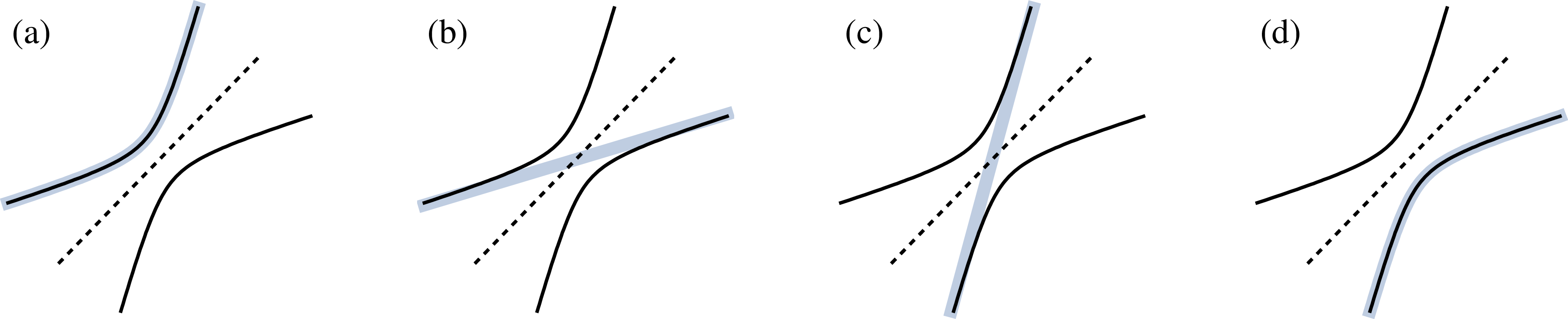

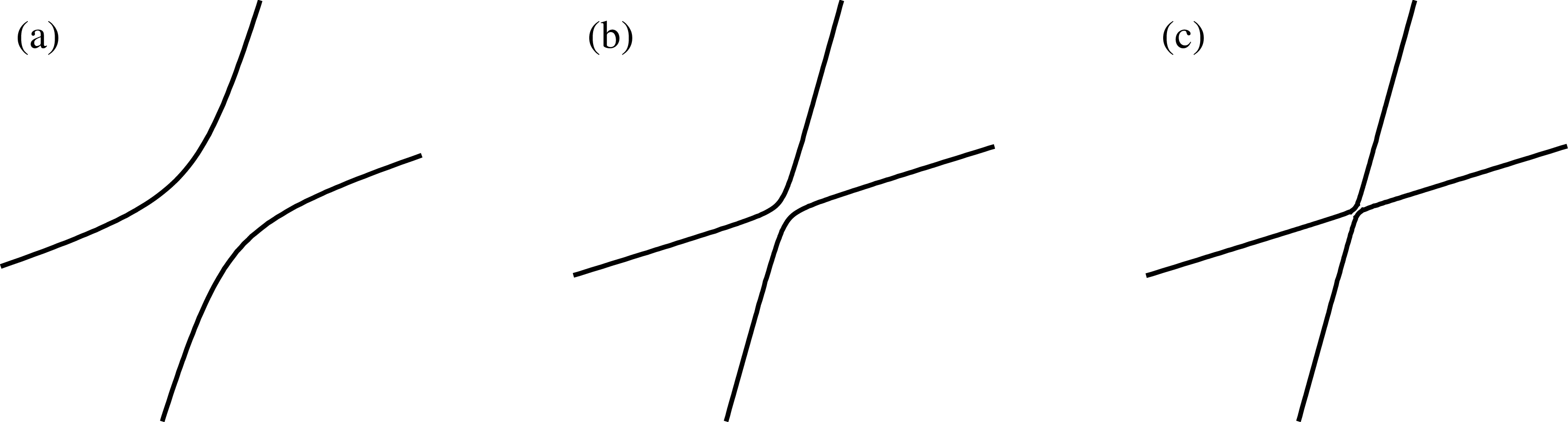


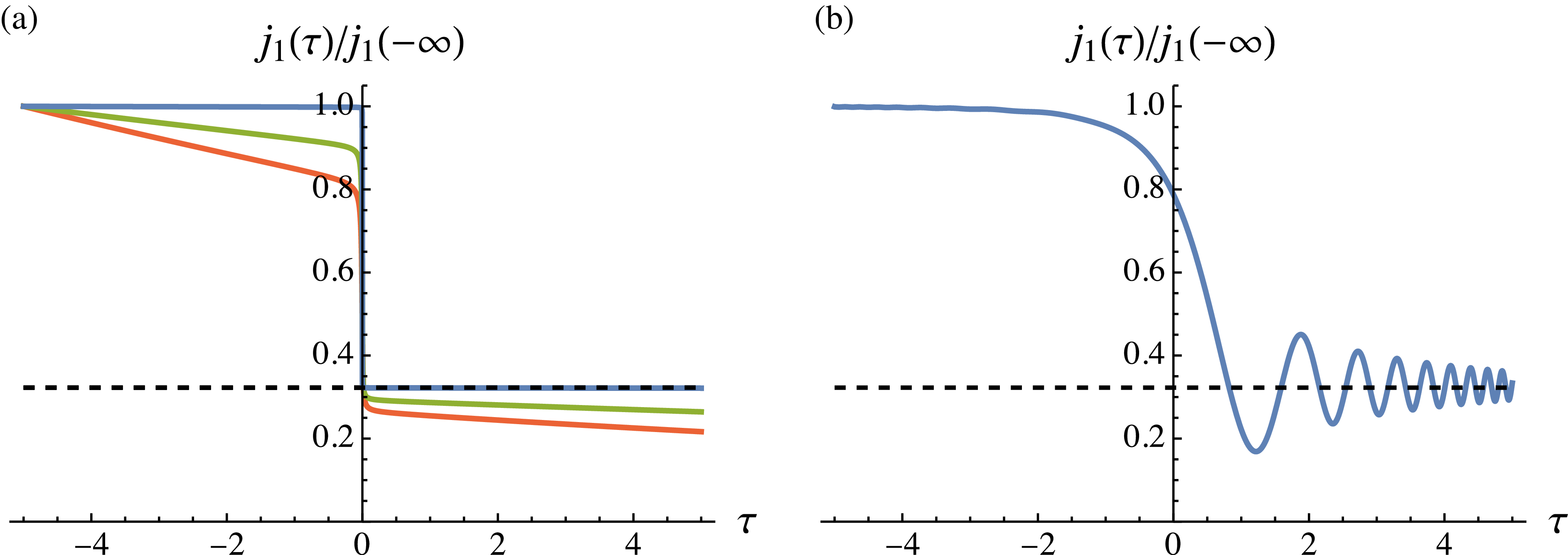


 Open access